

INTRODUCTION
Sea ice covers a large part of the Arctic Ocean. It works as insulation between relatively warm ocean water and cold air in winter. One of the important features of the ice cover is the presence of sea-ice leads. Leads are areas with open water or thin ice, which are usually of elongated shape. They appear as result of ice fracturing due to shear and divergence stresses in the sea-ice cover. These stresses are forced by the ocean currents, tides and to a large degree by winds in the atmosphere. Leads regulate the heat, gas and moisture exchange fluxes between the ocean and the atmosphere and are places of increased sea-ice production, during periods of freezing conditions. Hence, the spatial and temporal distributions of leads are of interest for climate studies (Maykut, Reference Maykut1978; Wang and others, Reference Wang, Danilov, Jung, Kaleschke and Wernecke2016). Furthermore, the mapping of sea-ice leads plays an important role for navigation providing an easier way for vessels through the pack ice. Also, leads are areas of increased biological activity in the ocean like phytoplankton blooms (Assmy and others, Reference Assmy2017). The life of Arctic animals (e.g. walruses, polar bears, birds) is often tied to leads.
Due to harsh weather conditions in the Arctic, capabilities for field studies of sea ice are limited. Remote-sensing methods can provide measurements in the Arctic covering large areas. Airborne and satellite instruments allow one to receive data with different spatial and temporal resolutions. Several methods were developed for discrimination of sea ice and water based on remote-sensing observations taken in the visible, infrared, and microwave parts of the electromagnetic spectrum. They are described in the following four paragraphs.
A large number of advanced very-high resolution radiometer (AVHRR) infrared images were analysed by Lindsay and Rothrock (Reference Lindsay and Rothrock1995) to determine lead characteristics. The lead detection algorithm is based on the concept of ‘potential open water’, a scaled version of the surface temperature or albedo that weights thin ice by its thermal or brightness impact. A threshold was set to discriminate open water from sea ice. The resolution of the data is about 2–3 km. In the studies conducted by Willmes and Heinemann (Reference Willmes and Heinemann2015, Reference Willmes and Heinemann2016), MODIS thermal infrared imagery was used for lead detection. The method is based on a threshold applied to MODIS images with the background subtracted. The resulting maps with resolution of 1 km contain three classes: sea ice, leads and lead-like structures. Both the AVHRR and MODIS-based methods are affected by cloud contamination.
The cloud influence is significantly reduced for observations in the microwave spectrum, where weather conditions have little influence on measurements. Lead detection based on microwave altimetry was studied by Wernecke and Kaleschke (Reference Wernecke and Kaleschke2015) using data from CryoSat-2. The algorithm to discriminate leads from ice is based on the maximum power, the pulse peakiness, and other parameters (e.g. the leading edge width, the trailing edge width, the stack standard deviation, and the stack excess kurtosis) of the reflected altimeter signal.
Estimations of lead concentrations and their orientation statistics were shown by Röhrs and Kaleschke (Reference Röhrs and Kaleschke2012) and Bröhan and Kaleschke (Reference Bröhan and Kaleschke2014) based on observations of the passive microwave imager AMSR-E. For AMSR-E data on a 6.25 km grid, they detect leads wider than 3 km, which results in a detection of 50% of the lead area that can be seen on MODIS optical images.
Synthetic aperture radar (SAR) is able provide high-resolution data with large spatial and temporal coverage. It is widely used for sea-ice-type classification and ice--water discrimination (Dierking, Reference Dierking2010, Reference Dierking2013). Ivanova and others (Reference Ivanova, Rampal and Bouillon2016) used a threshold approach on the HH-band (HH: transmitting and receiving in horizontal polarization) of the ENVISAT ASAR instrument for water--ice discrimination. To improve the quality of object classification the directly measured data (e.g. backscatter intensities) are often extended with textural features. Ice--water classification based on dual-polarised SAR images (RADARSAT-2) with the additional texture information is described by Leigh and others (Reference Leigh, Wang and Clausi2014). The use of a support vector machine on the features based on the grey-level co-occurrence matrix (GLCM) (Haralick and others, Reference Haralick, Shanmugam and Dinstein1973) is suggested. This combination was previously used for sea-ice-type classification by Liu and others (Reference Liu, Guo and Zhang2015), Korosov and Park (Reference Korosov and Park2016). A similar approach is used by Zakhvatkina and others (Reference Zakhvatkina, Korosov, Muckenhuber, Sandven and Babiker2017) for ice--water discrimination. A neural network with texture features based on the GLCM was used for classification of ENVISAT SAR images by Zakhvatkina and others (Reference Zakhvatkina, Alexandrov, Johannessen, Sandven and Frolov2013). Another method that provides complementary information to the backscatter intensity is based on polarimetric features (e.g. Moen and others, Reference Moen, Anfinsen, Doulgeris, Renner and Gerland2015). Polarimetric features are used for sea-ice classification (e.g. Ressel and others, Reference Ressel, Singha, Lehner, Rosel and Spreen2016), iceberg detection (Dierking and Wesche, Reference Dierking and Wesche2014) and oil spill recognition (e.g. Brekke and others, Reference Brekke, Holt, Jones and Skrunes2014).
In this study, Sentinel-1 dual-channel C-band SAR measurements (co- and cross-polarised modes, HH and HV) are used. It should be noticed that several definition of a lead can be found in the literature (Weeks, Reference Weeks2010). Although leads often defined as elongated areas with open water, here we do not consider the shape of detected objects. The automatic lead detection algorithm we have developed is based on the analysis of backscatter amplitude and texture and, therefore, thin ice and open water between ice flows might be classified as leads. We combine polarimetric and texture features to produce sea-ice lead maps that, if combined, can cover the complete European Arctic. We investigate the optimal number of texture features for lead classification and provide the precision–recall curve as a classification quality metric. Results are evaluated by high-resolution (10 m) optical data from Sentinel-2.
DATA AND METHODS
Satellite data
The data used in the present study are listed in Table 1. For this study, we focused on two satellite constellations: Sentinel-1 SAR data are used for the lead detection and Sentinel-2 optical data as evaluation dataset. The data are available at the Copernicus Open Access Hub (scihub.copernicus.eu). The Copernicus Sentinel-1 mission currently comprisestwo satellites with a SAR as primary instrument. In the Extra Wide swath mode, SAR images are acquired at both HH and HV polarisations. The backscatter of the electromagnetic wave transmitted at 5.4 GHz frequency at horizontal polarisation is received and decomposed into horizontal (HH) and vertical (HV) polarisation components. The swaths width is 400 km, the resolution is 93 × 87 m (pixel size is 40 × 40 m). The typical size of a Sentinel-1 image is 10 000 × 10 000 pixels. Preprocessing of the data includes thermal noise removal, incidence angle correction and speckle noise filtering. The flowchart of the lead detection algorithm is shown in Figure 1. Thermal noise and correction parameters, which are provided in the auxiliary data, are applied to the SAR images according to the equation given in the Sentinel-1 processing chain documentation (ESA, 2016):
 $$\sigma = {\displaystyle{(\,pixel\; value^2 - noise)} \over {\gamma^2}}$$
where pixel value is the amplitude of backscatter of the original HH or HV band, noise is the intensity of the thermal noise and γ is a calibration coefficient, noise and γ are provided in the metadata. In the next step, the corrected backscatter is translated to dB by application of log 10. To prevent infinitely low values a threshold of 1/max (γ) has been applied as a limit. In this way, the thermal noise is removed from the SAR data, but the so-called scalloping noise remains. The effect of the scalloping noise is mainly visible over the open ocean and therefore can be masked out with a sea-ice mask. A sea-ice mask can be retrieved by applying a threshold to a sea-ice concentration product. In this study, we use a 20% sea-ice concentration threshold for the ASI AMSR-2 algorithm [seaice.uni-bremen.de](Spreen and others, Reference Spreen, Kaleschke and Heygster2008).
Processing flowchart; LV stands for local variability (image with background subtracted).
List of Sentinel-1 and -2 products used in the study
The last column gives the fraction of the satellite scene in per cent that is used for the classification training and testing.
Backscatter of sea ice in the HH band of SAR data is known to depend on the elevation angle (and, consequently, incidence angle), which therefore should be taken into account. A linear regression of HH backscatter versus elevation angle is used. The regression coefficients are derived from a set of 16 extra wide swath mode products with homogeneous areas acquired over sea ice. These products cover the entire range of incidence angles used in the extra wide swath mode. The resulting equation for the incidence angle correction is
 $$\sigma_{new} = \sigma + 0.049 \cdot (\theta - \min{(\theta)})$$
where σ new is the backscatter after the correction, given in dB, and θ is elevation angle in degrees. The HV band does not reveal a significant sensitivity to the incidence angle; therefore, the correction is done only for the HH band. The next step of the preprocessing is the reduction of speckle noise. A bilateral filter is applied, which is an edge-preserving filter known to have good performance in reducing speckle noise (Tomasi and Manduchi, Reference Tomasi and Manduchi1998; Alonso-Gonzalez and others, Reference Alonso-Gonzalez, Lopez-Martnez, Salembier and Deng2013). The size of the square window of the filter was set to 5 pixels. With this the preprocessing of the Sentinel-1 data is finished.
The second source of satellite data used in this study are observations from the Sentinel-2 satellite constellation carrying a multispectral instrument with 13 bands in the visual and near-infrared spectral range. Images with a spatial resolution of 10 m for visual and 20 m for near-infrared are used for comparison with SAR images to evaluate the results of the lead detection algorithm.
Training and evaluation datasets
To train the classifier datasets are needed with correctly identified objects, i.e. in our case leads with thin ice or open water. We use a manual classification of six Sentinel-1 scenes that cover two different typical lead appearance types: dark and bright leads (three scenes for each of the two cases). These scenes are taken from different times of the year (Table 1). No scene from summer was used for training datasets because during the melt season melt ponds can have similar signature in SAR backscatter as leads with open water. To evaluate the results of the classification on independent data, two cases of overlapping Sentinel-1 SAR and Sentinel-2 optical data are used (Table 1). Although images in one of the cases were taken in August, there is no evidence of melt ponds presence on them. Hence, the melt season is excluded from the study.
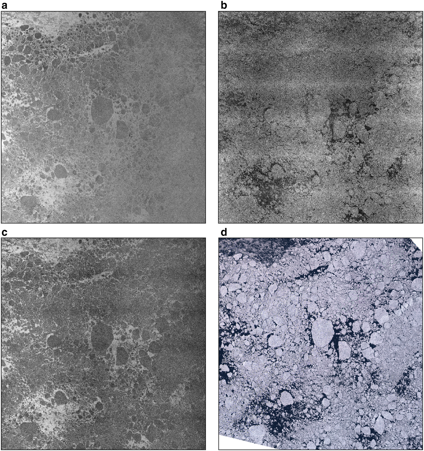
Leads with open water or thin ice in most cases have low surface roughness and therefore have low backscatter values on both SAR bands, HH and HV. They appear dark on the optical image used for evaluation as well. This case is represented in the first of the two evaluation datasets. Figs 2a, b and c show the HH, the HV and the product of SAR bands HH·HV, respectively, and Figure 2d the Sentinel-2 image of the corresponding area taken in the visible spectrum. The time difference between the acquisitions is 7 h 40 min. Most areas covered with leads appear dark on all images. Only around edges of leads thin crushed ice with a high surface roughness can appear bright while on the image taken in visible spectrum the same thin crushed ice is transparent. The assumption for using the band product HH·HV is that if either the HH or HV band show low backscatter intensities the band product will have low values.
Panels (a) and (b) are HH and HV bands. (c) Product of the HH and HV bands (HH·HV) of the SAR scene taken on 10 April 2017, west of the Franz Josef Land. (d) Optical data from Sentinel-2 taken on 10 April 2017, west of the Franz Josef Land.

Leads with open water, however, can appear bright on HH band under high incidence angles if wind roughens the water surface (Scharien and Yackel, Reference Scharien and Yackel2005). In the HV band, leads appear dark under the same conditions. Thin sea ice with frost flowers in leads can have high backscatter values in both HH and HV bands (Nghiem and others, Reference Nghiem1997; Dierking, Reference Dierking2010; Isleifson and others, Reference Isleifson2014) and therefore can look like pressure ridges in C-band images. They might not always be classified correctly here. However, lead detection from the HV band is more prone to errors since the backscatter intensity at HV band is low and often close to the noise floor. An example of the situation when leads have high HH band backscatter intensities is shown in Figs 3a, b and d for Sentinel-1 HH, HV and Sentinel-2, respectively. Leads that are clearly observed in the optical data look brighter than the surrounding sea ice at HH band from SAR and darker in the HV band. In the band ratio HH/HV image leads appear bright if HH is high and HV is low.
Panels (a--c) are HH, HV bands and band ratio, respectively, of a Sentinel-1 SAR scene taken on 2 August 2016, between Svalbard and Franz Josef Land; (d) Optical data from Sentinel-2 taken on 2 August 2016, between Svalbard and Franz Josef Land.
To account for these two different situations, we therefore split the lead classification algorithm into two parts: the first one detects leads that appear dark on both SAR bands, the second one is used for cases with high backscatter values at HH band (compare also the two branches in the flowchart in Fig. 1). In the last step, both outputs are merged to produce the final lead map.
Two cases of overlapping Sentinel-1 and -2 data, presented in Figures 2 and 3, are used for the evaluation of our algorithm. Here leads are marked by hand on the SAR dataset taking into account the corresponding optical Sentinel-2 images to confirm the validity of the selected leads.
For the training of the algorithm six other independent Sentinel-1 scenes are used (Table 1). They also represent the two cases of dark and bright leads in the HH band, respectively. Three scenes are used to train the dark lead classifier and three other scenes to train the bright lead classifier. No optical Sentinel-2 data are available for these six scenes. Therefore, leads were identified and marked manually in the six Sentinel-1 scenes without the additional support from optical data. The later six images are used as training and test datasets, final evaluation is performed on SAR images which overlaps with optical data shown in Figures 2 and 3.
Texture and polarimetric features
In addition to the measured HH and HV backscatter intensities, the feature space for object classification in SAR images can be extended by two methods: polarimetric and texture features. Polarimetric features can be used for SAR products containing at least two out of the four Stokes vector components whereas texture features can be calculated for a single polarisation band. Here we combine the two approaches for Sentinel-1 dual-polarisation data. Products of the Sentinel-1 extra wide swath mode used in the Arctic contain co- and cross-polarised bands (HH and HV). As only the amplitude but not phase is available for our data source, the number of available polarimetric features is restricted. In this study, the product HH·HV and the ratio HH/HV are used as polarimetric features. The co-polarisation ratio HH/VV and real part of the co-polarisation cross-product is widely used for the SAR image classification Brekke and others (Reference Brekke, Jones, Skrunes, Holt and Espeseth2016). It have shown good performance in discriminating open water from sea ice (Ressel and others, Reference Ressel, Singha, Lehner, Rosel and Spreen2016). In the absence of VV, we use HV instead. The cross-polarisation ratio was used for classification of SAR images by (Karvonen, Reference Karvonen2014) Bright, wind roughened leads in HH appear dark in HV (Fig. 3), which will cause high values in HH/HV and this is the case we like to detect with the band ratio. The classification for dark leads is based on the HH·HV product, which will be low if one of the channels is low, i.e. dark. However, because of the low signal-to-noise ratio in the HV band the classification based on the band product is also compared with the classification based on the HH band alone to quantify if there is a benefit from the use of both bands.
Therefore, the HH band, the HH·HV product and the HH/HV ratio are used as input for the following texture analysis. Figures 2c and 3c show examples of the band product and ratio, respectively.
Texture features based on the GLCM are widely used for classification of SAR data (Haralick and others, Reference Haralick, Shanmugam and Dinstein1973; Leigh and others, Reference Leigh, Wang and Clausi2014; Liu and others, Reference Liu, Guo and Zhang2015; Zakhvatkina and others, Reference Zakhvatkina, Korosov, Muckenhuber, Sandven and Babiker2017). The complexity of texture feature calculation depends on the size of the chosen sliding window and the number of grey levels of the input image. Here a discretisation into 16 grey levels has been chosen as trade-off between conservation of details and computational cost. GLCMs are then calculated for a sliding window of 9×-pixel size with 1 pixel step size. A bilinear weighting within the sliding window was applied, so that pixels which are closer to the middle of the window have higher weight for the GLCM computation.
The 12 GLCM features we use in this study are listed in Table 2. Definitions of the features are given by Haralick and others (Reference Haralick, Shanmugam and Dinstein1973). Some GLCM features depend on the image brightness (in our case the value of the HH and HV product or ratio). This means that the absolute value of the pixel brightness influences these texture features. Since leads are often darker than the surrounding sea ice, the difference between the original image and a low-pass filtered version of the image is calculated to show the small-scale backscatter variations. A bilateral filter with a 25 ×−pixel sliding window is applied to the preprocessed original image and subtracted from the non-filtered image. In this way, the local backscatter variability is emphasised and is used further as an additional information for the classification. Afterwards GLCM texture features are calculated both for (i) the original image and (ii) for the small-scale variations of the image. In this way, two sets of texture features are produced for each of two input polarimetric features (i) band product and (ii) band ratio, and for the HH band, and further analysed (see also flowchart in Fig. 1).
Twelve GLCM features are used in the study
Definitions of the texture features are given by Haralick and others (Reference Haralick, Shanmugam and Dinstein1973).
Supervised learning algorithms
We use the Random Forest Classifier (Breiman, Reference Breiman2001) implemented in scikit-learn library [http://scikit-learn.org/stable/index.html] (Pedregosa and others, Reference Pedregosa2011) for sea-ice lead detection. It is an ensemble method that constructs a set of decision trees. Each of these trees is trained on a different subset of data points and features. The decision made by each tree is weighted to provide the final result. The method has been proven to have good quality of classification and at the same time high computational speed. One of the advantages of the classifier is its internal metric for feature importance, which gives information on the frequency of use of each of the input features. Another advantage of the classifier is its capability to perform not only binary, but also probabilistic classification. The probability of pixels to belong to a class can afterwards be translated to binary classification based on a threshold. The default behaviour is the use of a threshold of 50% probability. Different thresholds can be applied to adjust the result of classification. While there are several metrics to evaluate the quality of an algorithm, the most widely used metric is accuracy (Eqn (3) below). Although alone it might be unrepresentative for the case when the size of one class is considerably larger than the size of the other class. Leads usually occupy a few per cent of sea-ice area in the Arctic (Steffen, Reference Steffen1991), so that additional metrics should be used for quantifying the classification performance.
Precision and recall scores are defined by Fawcett (Reference Fawcett2006) and are used in the present study altogether with accuracy.
 $$accuracy = {\displaystyle{TP + TN} \over {TP + FP + TN + FN}}$$
 $$precision = {\displaystyle{TP} \over {TP + FP}}$$
 $$recall = {\displaystyle{TP} \over {TP + FN}}$$
where TP stands for true positive (pixels correctly classified as a lead), TN – true negative (pixels correctly classified as not being a lead), FP – false positive (pixels that are not leads but are classified as a lead), FN – false negative (pixels that are leads but are classified as ‘not lead’) predictions. The sum TP + FP + TN + FN equals to the total number of pixel in the image. Accuracy can be explained as amount of correctly classified pixels over the total number of pixels. Precision is the amount of correctly classified pixels of the given class over the total number of pixels classified as the given class. Hence,  $(1 - precision) = {\scriptstyle {FP} \over {TP + FP}}$ is the number of sea-ice pixels misclassified as a lead over the total amount of pixels classified as leads. The recall rate characterises how complete the classification is, that is the number of samples classified correctly over the total number of samples of this class. These three scores provide the needed information on the quality of a given class classification. They can aid to make decisions on how many features are needed for the classifiers.
To describe what probability threshold gives the best results for a probabilistic classifier, the receiver operating characteristic curve and the precision–recall curve are widely used (Fawcett, Reference Fawcett2006; Davis and Goadrich, Reference Davis and Goadrich2006). The receiver operating characteristic, for example, was applied for the lead detection algorithm described by Wernecke and Kaleschke (Reference Wernecke and Kaleschke2015). Here we use the precision–recall curve to decide for an optimised binary threshold value for the Random Forest Classifier. This will be presented in the results section.
Two main parameters of the classifier that influence classification quality and computing time are the number of trees and the maximal depth of each tree. To choose the most suitable values for these parameters the six training SAR scenes, where leads were marked without support from optical data, have been used. The evaluation with the additional optical scenes will be presented later.
The two SAR datasets for the ‘dark’ and the ‘bright’ lead classifiers (three SAR scenes each) with manually identified leads have been randomly split into a training (25% of the data) and a test dataset (75% of the data) each. Two classifiers are trained on the scenes where leads appear dark in the HH band: one is based on the HH band, another one is based on the HH·HV product. Results of the two classifiers are compared later. The third classifier is trained using the HH/HV band ratio based on the scene where leads appear bright in the HH band. Each of the three classifiers are trained on the corresponding training dataset and then they are evaluated on the training and test datasets. A number of trees equal to 64 has been chosen for balance between efficiency and computing time. The maximal depth of trees was set to 15 to prevent overfitting and decrease computing time.
To decide how many texture features give positive benefit for the classification quality and to remove features that are not needed a so-called recursive feature elimination (RFE) is carried out. 12 texture features for the band data, 12 texture features for the small-scale variations of the band, and the original (preprocessed) band data altogether constitute 25 features which are used in the RFE. The Random Forest Classifier provides the rank of importance for all features used in the lead classification. Recursively, now after each training and classification the number of features is reduced by one and the training and the classification started again. After every step the texture feature with the lowest importance according to the classifier's metric (i.e. the feature least used) is eliminated. Accuracy, precision and recall are calculated to estimate the classification quality of the algorithm on the given subset of features. The operation is repeated until one feature is left. To calculate the three quality metrics a binary classification based on 50% probability threshold is used. Based on this experiment the optimal number of features can be chosen, which is presented in the next section.
RESULTS
Optimal number of texture features for classification
The procedure for texture feature ranking described in the last section was carried out three times: one time for the band product data (HH·HV), the second one for the HH band data and the third one for the band ratio (HH/HV). The band product and the HH band are used for the training dataset where leads appear dark and the band ratio on the training image with primarily bright leads. Table 3 lists the 25 texture features in the order they were eliminated for each of the three cases: (i) HH band, (ii) band product and (iii) band ratio.
Elimination order of texture features, i.e. the lower the number N the least important is the respective feature for the classifier

Indices o and ssv stand for the texture features calculated on the original image and the small-scale variations of the image, respectively (see the section ‘Texture and polarimetric features’). Definitions of the texture features are given by Haralick and others (Reference Haralick, Shanmugam and Dinstein1973). The three columns present the elimination order for the three classifiers based on (i) HH, (ii) band product and (iii) band ratio.
Accuracy, precision and recall scores in dependence on the number of features eliminated are shown in Figures 4a, b and c, respectively. Dashed lines show accuracy, precision and recall rates for the training set, solid lines are given for the corresponding metrics calculated on the test dataset. Blue lines stand for classification of the band product, green lines stand for classification of the HH band (i.e. dark lead cases) and red for the band ratio products (i.e. bright lead case).
Accuracy (a), precision (b) and recall (c) scores of the three classifiers depending on number of features eliminated during the RFE analysis. The scores are calculated for the training and test datasets for each of the three classifiers based on the band ratio(red), band product (blue) and HH band (green).
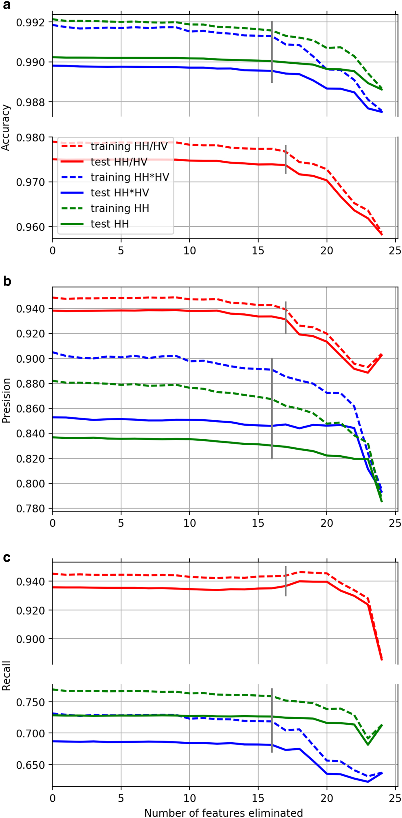
Accuracies of the three classifications stay almost constant until the first 9 texture features are eliminated. A noticeable decrease in the classification accuracy appears after 16 texture features are eliminated for both the HH and the band product classifiers and after 17 for the band ratio classifier. This indicates that the first 9 texture feature for each of the tree classifiers (Table 3) can be eliminated without any harm for classification and as little as 3 to 8 texture feature already can provide good classification results.
The precision and the recall rates of the HH band and the band product classifiers follow corresponding accuracy trends, but show more variation in amplitude. The recall rate of the band ratio classifier shows an increase after 17 texture features are eliminated, but at the same time the precision of the classification drops.
Although all the 25 features could be used for the lead classification, we remove the ones that do not show significant benefit for the classification result. Based on Figs 4a, b, c the number of texture features equal to 9 has been chosen for classification of the HH band and the band product, i.e. the first 16 texture features of the first and the second columns in Table 3 are removed from the classification. Although we keep only 9 of the texture features, it should, however, be noticed that one could use up to 16 features if even a little improvement of the classification quality is desired. For the band ratio the last 8 texture feature from Table 3 (the third column) are used for classification in further studies, the first 17 are removed from the band ratio classification.
Since the same dataset is used for both the HH and the band product classifiers, their performance can be compared. The accuracy of the HH band classification is only 0.2% higher than the accuracy of the band product classification. On the other hand, the band product classification shows a higher precision, but a lower recall comparing with the HH band classifier. Since we do not define whether precision or recall is more important for lead classification, we are not able to make a conclusion on which of the two classifiers shows a better classification quality at this point. In order to find which of the two classifiers, based on the band product and the HH band, shows better classification quality, the influence of a probability threshold on precision and recall and, therefore, on the lead classification is analysed in the next section.
Optimal probability threshold for classifiers
The Random Forest Classifier can provide probabilistic classification, which can be analysed as is or be used to obtain the corresponding binary classification by setting a threshold. Here we study the influence of a threshold used to produce the binary classification on the classification quality.
Three probabilistic classifications of the test data were produced with the three classifiers based on the HH band, the band product HH·HV and the band ratio HH/HV. Than a range of threshold is applied to each of them to receive the corresponding binary classification.
To describe the influence of the threshold, the precision–recall curves are calculated for each of the three classifiers (shown in Fig. 5). Dashed lines correspond to precision–recall curves calculated for the training dataset, solid lines are calculated for the corresponding test dataset. Red lines represent the quality of the classifier based on the band ratio which is used for the bright lead detection. Blue and green lines represent qualities of classifiers based on the band product and the HH band, respectively. The numbers in black give the respective threshold values used. A higher threshold improves the precision score (i.e. reduce amount of misclassification) but at the same time lowers the recall score (reduce the number of lead pixels detected).
Precision–recall curves calculated for the training (dashed) and the test (solid) datasets corresponding to three classifiers: based on the band product (blue), the HH band (green) and the band ratio (red). The curves are obtained by applying different thresholds to a probabilistic classification. The points on the curves which correspond to the threshold values of 30, 50, 70 and 90% are denoted in the figure (0.3, 0.5, 0.7 and 0.9, respectively).
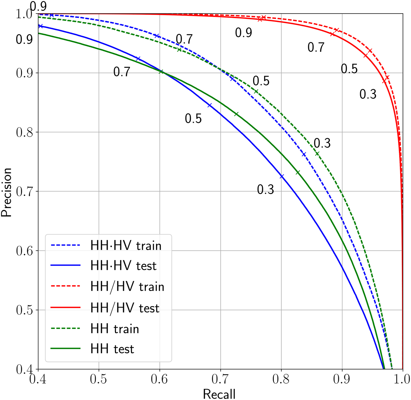
From Figure 5 it can be seen that leads are classified with only 84 and 83% precision on the band product and the HH band if the default threshold of 50% probability is used (the solid blue and the solid green curves). But in this case 68 and 72% of all pixels belonging to the lead class are identified (the recall score). If the threshold is set to 70%, then only 57 and 60% of the lead pixels will be detected, but precision of the classification is 92 and 90% (for the band product and the HH band, respectively). To identify more lead pixels the threshold can be lowered. For example, the threshold set to 30% will allow to detect 80 and 82% of all pixels belonging to leads, but the precision of the classification will drop to 72 and 73%, respectively, for the two classifiers HH and HH·HV.
Similarly, threshold can be adjusted for the classification of the band ratio. The default value 50% will give 93% precision and 94% recall, the higher value, 70% for instance, will increase precision to 97% and decrease recall to 88%. The lower threshold value of 30% will produce the binary classification with 88% precision, up to 97% of lead pixels will be identified.
The solid blue and the solid green curves intersects at the point where precision is 90% and the recall rate is 60%. This means that the two classifiers show the same classification quality for the corresponding two threshold values of the two classifiers. For a higher threshold value, a higher precision can be achieved with the same recall rate value if the band product classification is used with the appropriate threshold value. Let us consider the right part of precision–recall curves where the green curve is above the blue. It corresponds to an application where the amount of leads detected (the recall rate) is more important than a very high precision (which is lower than 90% in this part of the curve). In this case, for any value of the recall rate the binary classification based on the HH band shows better precision (when a certain threshold is applied to the probabilistic classification) than the binary classification based on the band product.
The opposite is true for the left part of precision–recall curves where the blue solid line is above the green one (i.e applications where a high precision is important). Based on these curves one can chose the appropriate threshold value for a certain task. For example, in climate studies about heat balance and energy one would want to have as many leads detected as possible although some of the detections are wrong. On the other hand for navigation, it is more important to know the location of leads with the highest precision possible even though the number of leads detected is lower.
Evaluation
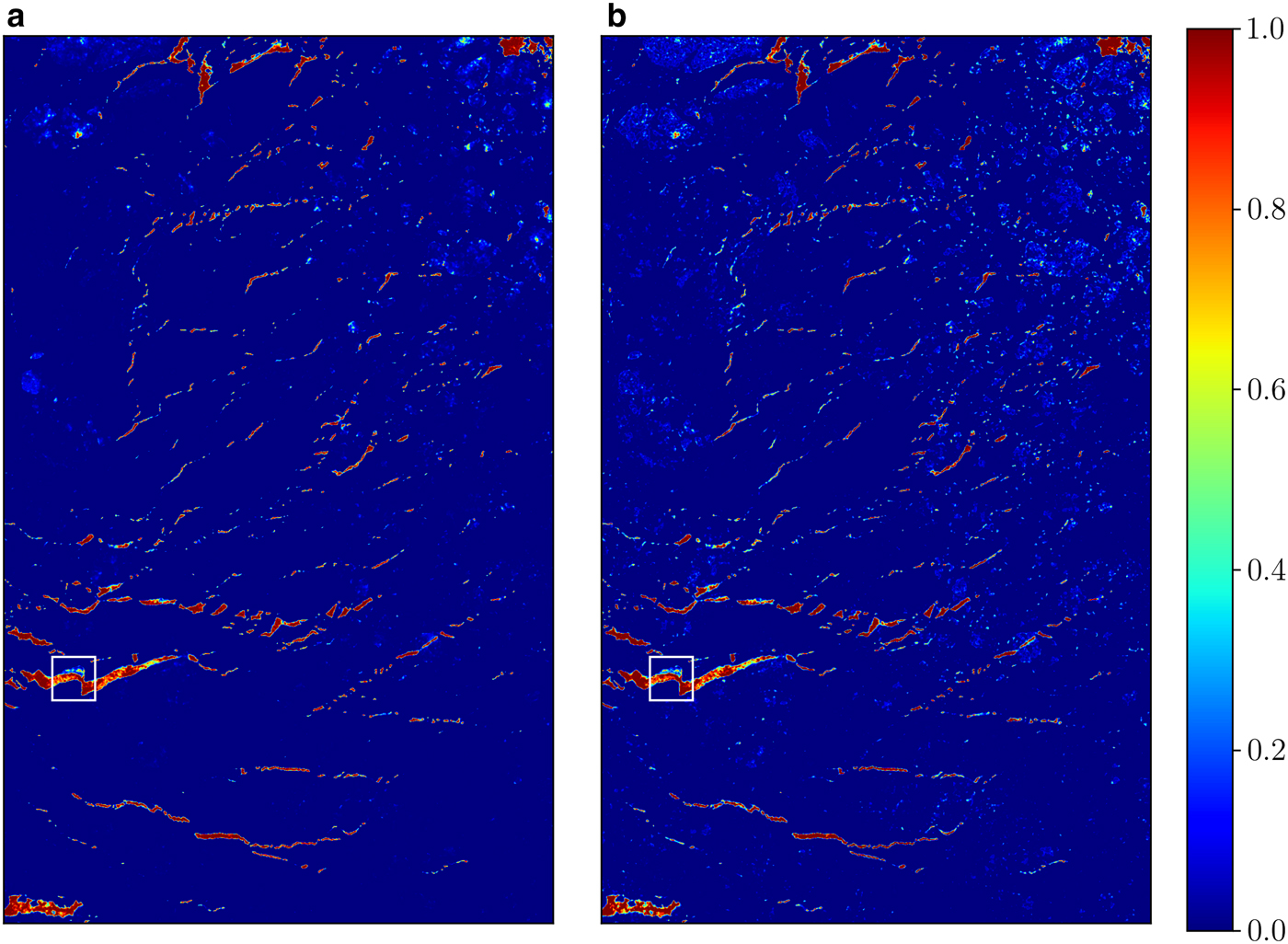
So far, only results based on the Sentinel-1 SAR data without overlap with optical Sentinel-2 data have been presented. In this section, an evaluation of the leads classification quality is conducted for the two Sentinel-1 SAR scenes which overlap with optical Sentinel-2 data (Figs 2 and 3). Two probabilistic classifications of the first evaluation image (Fig. 2) were produced. The first one is based on the HH band (Fig. 2a), the second is based on the band product (Fig. 2c); 9 of the most important texture features (last 9 features in the first and the second columns in Table 3) were used in both cases. Results are shown in Figure 6. High probabilities of leads are assigned to areas which can be considered as leads from the optical image. Edges of leads have lower probability comparing to their inner parts. This effect is expected because the classification is based on texture features which are calculated within a window around each pixel. Some ice floes that appear dark on SAR images have non-zero probability values, but can easily be distinguished from leads. The upper part of a lead (the white frame at Figs 6a and b) has a significantly lower probability because it is covered with new ice as it can be confirmed from the optical data (Fig. 2d). Large leads are detected correctly, but thin leads (up to 10 pixels which corresponds to 400 m) are often split into several small pieces. Leads with width <5 pixels (200 m) are smoothed on the step of texture features calculation. As the result such leads have low probabilities and can be considered as not-detected. This is a disadvantage of the method which cannot be eliminated because to calculate texture features relevant for a lead, the lead should have a size comparable or larger than the window size used for texture feature computation.
Probabilistic classifications of the SAR scene shown in Figure 2c performed with the Random Forest Classifier. Panels (a) and (b) are classifications based on the HH and the band product, respectively. High values mean high probability of a pixel to be classified as a lead.
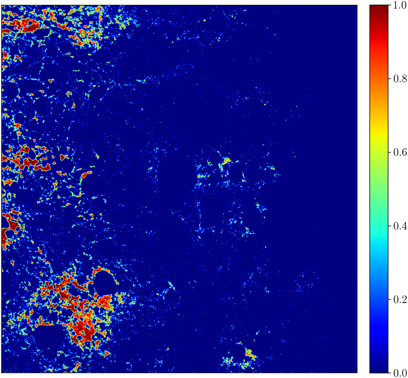
The probabilistic classification of the second evaluation image (Fig. 3c) for the band ratio was performed with 8 input features. Figure 7 shows the result of the probabilistic classification. Many open water areas at the left side of the scene are classified as leads while in the middle leads are not detected. This can be explained by the fact that leads are more pronounced at the left side of the band ratio (Fig. 7c) which was used as input for the algorithm. The fact that areas which are classified as leads are covered with open water can be confirmed from the optical observation (Fig. 7d).
A probabilistic classification of the scene shown in Figure 3c performed with the Random Forest Classifier and based on 8 texture features.
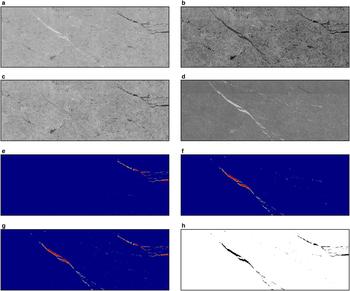
The following example illustrates the algorithm for lead detection (the flowchart for the algorithm is shown in Fig. 1). The original Sentinel-1 SAR images are shown in Figs 8a and b. One can observe two large elongated objects, one is dark on both the HH and the HV bands, the other one is bright on the HH and dark on the HV band. The two objects represent the two classes of leads we have introduced here, ‘bright’ and ‘dark’ leads. No optical data are available for the scene to confirm that the objects are leads, and we can only rely on our experience of how leads appear in SAR images.
Panels (a) and (b) are the original HH and HV bands. (c, d) The band product and the band ratio derived from the HH and HV bands. (e, f) Probabilistic classifications of the SAR scene based on the band product ratio performed with the Random Forest Classifier. High values means high probability of the pixel to be classified as a lead. (g) The sum of the two probabilistic classification. (h) Binary classification based on (g) with 50% probability threshold applied.

To classify both types of leads, two classifiers are applied – one for the dark lead detection and one for the bright lead detection. At first, based on the HH (Fig. 8a) and the HV (Fig. 8b) bands, the band product (Fig. 8c) and the band ratio (Fig. 8d) are calculated. Dark leads are detected from the band ratio using the algorithm based on either the HH band or the band product (the result based on the band product is shown in Fig. 8e). Bright leads are detected with the algorithm based on the band ratio (Fig. 8f). Afterwards, the probabilities for the darkand the bright lead branches are added together. As the last step, a threshold of 50% is applied to the resulting probabilistic classification, so that the final binary classification is obtained (Fig. 8h).
DISCUSSION
Texture features for classification
The procedure of texture features elimination shows that the use of a range of texture features (the first 9 from each column of Table 3) do not improve the classification and therefore can be excluded from it. At the same time these texture features do not decrease classification quality. This is because although these features are feed to the classifier, only the texture features that help to perform classification are used within the Random Forest Classifier. In the process of elimination of the next 7–8 texture features, the classification quality slightly decreases. Therefore these 7–8 texture features may also be excluded from the classification process, especially if fast computation is of importance. As the result 16–17 texture features can be eliminated without significant decrease in classification quality, so that only 8–9 of the texture features are used in classification. In cases when even a little improvement of the classification quality is desired, up to 16 input features can be used. For the case when computational time is limited, the number of texture features used for classification can be decreased.
Of the 9 most important texture features (last 9 rows in Table 3) the majority was derived from the original input band and not from the small-scale variations data, where the background amplitude was removed. The original band is one of the most important inputs for all three classifiers. This means that texture features cannot substitute the original band and provide complementary information. Texture features and the original band should be used in conjunction.
To produce the final lead map a classifier based on either the band product or the HH band for dark leads should be used in combination with the classifier based on the band ratio for bright leads. In Figure 4b, the classifier based on the band product shows higher precision; however, in Figure 4c the recall rate of the classifier is lower compared with the classifier based on the HH band. This leads us to the conclusion that both the precision and the recall by itself do not provide enough information about the quality of a classification, neither of the two should be used as the only quality metrics, and both of them should be considered together.
In case of probabilistic classification, it is possible to increase the precision by the cost of the recall rate and vice versa by adjusting a threshold used to obtain the corresponding binary classification. Thus, a comparison of the two classifiers is performed by the use of the concept of the precision–recall curve.
Classification quality
Let us consider the quality of dark leads classification first. The precision–recall curves (Fig. 5) of the HH and band product classifiers have an intersection point. This means that each of the two classifiers could be considered as the one that should be used in the final product. The quality of the classifier based on the band product is higher when a high precision (over 90%) of lead detection is desired. In this case, only about 60% or less leads will be detected. If the recall rate also matters for the application, the HH band should be used for dark leads classification.
The precision–recall curves clearly show that the quality of bright leads classification is higher than of the dark leads classification based on both the band product and the HH band (red curves are above blue and green curves). This might be due to the fact that sea ice can appear dark at both the HH and the HV bands and might be misclassified as a lead. At the same time, the band ratio is known for its good water--sea-ice discrimination potential. Objects, that appear bright at the HH band and dark at the HV band are usually not misclassified as sea ice (which can be dark or bright at the both bands) or pressure ridges (bright at both bands). This gives us more confidence that an object detected from the band ratio is a lead.
In case of single-band measurements only the HH band is available for Sentinel-1 images taken in the extra wide swath mode. This single-band mode is often used for scenes at high latitudes. In this case, only the HH classifier for dark leads can be applied. If dual-band SAR data are available, we are able to calculate the band product and band ratio and therefore to use the classifiers based on HH·HV and HH/HV. The first classifier shows better classification quality for dark leads than the classifier based on the HH band (Figs. 4 and 5) when used for a high-precision classification (with precision above 90%). Since bright leads show a similar backscatter as ridges in HH band, they cannot be detected from HH band alone. Thus, with the use of the band ratio more leads are detected from the dual-band SAR data than from single HH band data.
As the lead detection algorithm is based on backscatter analysis, water between ice floes is classified as leads. During summer the separation of leads from melt ponds will not be possible with the features used here (the shape of the features would have to be taken into account). For the data used in this study there is no evidence for the presence of melt ponds. Therefore the algorithm has not been evaluated for the summer season. The ability of lead classification during the melt season is the subject of future studies.
SUMMARY
In this study, we developed a lead classification algorithm that can be applied to Sentinel-1 SAR dual band products. To account for the variability of SAR lead signatures in C-band backscatter, two classifiers, one for leads appearing dark (a classifier based on either the HH band or the band product can be used) and one for leads appearing bright in SAR imagery, were trained. The polarimetric features, the band product HH·HV and the band ratio HH/HV as well as the HH band, were extended with 24 texture features each. The texture features are based on the GLCM: 12 of them are calculated for the polarimetric feature directly and another 12 are derived from the small-scale variations of the polarimetric feature. Together with the original polarimetric feature this yields 25 different features that can be feed into the classifier (see Table 3). A RFE procedure showed the texture feature importance for the classification of leads. We found that although all 25 input features can be used, decreasing of their number does not always leads to a decrease of the classification quality. As little as 3 texture features can already provide useful classification of leads. Classifications with 9 texture features for dark and bright leads already show good classification quality and therefore were used further in this study. More features did not significantly improve the classification results.
Precision–recall curves were calculated for the three classifiers based on the HH band, the band product and the band ratio. For classification of dark leads in the domain of high precision and low recall rates (precision above 90% and recall below 60%) the classification based on the band product shows better quality than the classification based on the HH band. However, when the amount of leads detected is important, the classifier based on the HH band shows better quality and therefore is preferred. The classifier based on the band ratio, allows us to identify bright leads that can be detected only if dual band SAR images are available. Therefore, more leads are identified from the combination of the HH and the HV bands comparing to the single HH band SAR product. The classifier is able to identify leads with a high precision of above 95% for bright leads and above 90% for dark leads when 70% of all leads are detected. The overall precision is between the two and depends on ratio of dark and bright leads. The ratio depends on combination of the lead distribution, incidence angle, time difference between formation of a lead and acquisition of image over the area with the lead. The precision can be increased by the cost of the amount of leads detected (Fig. 4). The classification of leads from SAR is confirmed by optical imagery from Sentinel-2. Under some circumstance, however, to achieve such high precision the percentage of the total leads area identified (recall score) can drop to 60% and lower if a higher precision is desired. The advantage of the presented method is that the interplay between precision and recall score can be easily adjusted depending on the application.
The lead detection method presented in this paper has proven to be stable in our tests and the eight SAR scenes presented here (Table 1). In a next step, we will apply this method to a larger amount of Sentinel-1 SAR scenes. The spatial and temporal coverage of Sentinel-1 data in the Arctic will result in lead maps of the European Arctic on a daily basis. With the now operational two Sentinel-1 satellites, a and b, the complete Arctic Ocean is covered at least once per week. The Sentinel-1 time series is still short but we expect that lead statistics can already be derived for the first years and extended in future.
ACKNOWLEDGMENTS
This study was supported by the Institutional Strategy of the University of Bremen, funded by the German Excellence Initiative, and by the Deutsche Forschungsgemeinschaft (DFG) through the International Research Training Group IRTG 1904 ArcTrain. We gratefully acknowledge the provision of Copernicus Sentinel data [2015–2017] provided by the European Union via the Copernicus Open Access Hub (scihub.copernicus.eu).


 Open access