2.0 EULER’S DYNAMIC EQUATIONS FOR THE MOTION OF A RIGID BODY

The spacecraft systems with constant values of the principal moments of inertia are considered first. For their analysis, the Euler dynamic equations of motion of the rigid body are used^{(Reference Wie7)}:

(1)\begin{equation}\left\{\begin{array}{l} {I_{xx}}{\mkern 1mu} {\mkern 1mu} {{\dot \omega }_x} = ({I_{yy}} - {I_{zz}}){\mkern 1mu} {\mkern 1mu} {\omega_y}{\mkern 1mu} {\mkern 1mu} {\omega_z}\\[4pt] {I_{yy}}{\mkern 1mu} {\mkern 1mu} {{\dot \omega }_y} = ({I_{zz}} - {I_{xx}}){\mkern 1mu} {\mkern 1mu} {\omega_z}{\mkern 1mu} {\mkern 1mu} {\omega_x}\\[4pt] {I_{zz}}{\mkern 1mu} {\mkern 1mu} {{\dot \omega }_z} = ({I_{xx}} - {I_{yy}}){\mkern 1mu} {\mkern 1mu} {\omega_x}{\mkern 1mu} {\mkern 1mu} {\omega_y}\end{array}\right.\end{equation}

These differential equations can be easily solved numerically providing that particular initial conditions are specified. One of the possible techniques is based on the Runge-Kutta methods, implemented in MATLAB and Cleve Moler, founder of Mathworks^®, provides interactive tools to implement this strategy^{(Reference Moler8)}. Another possibility is to re-write Eqs. (1) in terms of the quaternions and solve these resultant equations.

3.0 NON-DIMENSIONAL FORMULATION OF THE EQUATIONS

For the main derivations in this paper it will be typically assumed that the system has three distinct principal moments of inertia, which are arranged in the following order: I_xx < I_yy < I_zz. For more generic formulations, two non-dimensional parameters, η and ξ, both restricted in their values within the range between 0 and 1 are introduced:

(2)\begin{equation}\eta = {{{I_{xx}}} \over {{I_{zz}}}};\quad \quad \xi = {{{I_{yy}} - {I_{xx}}} \over {{I_{zz}} - {I_{xx}}}};\quad \quad (0 \lt \eta \lt 1;\quad 0 \lt \xi \lt 1)\end{equation}

Parameter ξ in this case would have a similar meaning of the non-dimensional coordinate counterpart from the Finite Element Method, defining the current position within the finite element. In the context of this study, ξ is specifying the non-dimensional relative position coordinate of the intermediate value of the moment of inertia between the minimum value of the moment of inertia I_xx and the maximum value of the moment of inertia I_zz. In other words, it can be said that ξ is the non-dimensional parameter in the Hermite functions, enabling calculation of I_yy using I_xx and I_zz, using the following relationship:

(3)\begin{equation}{I_{yy}} = {I_{xx}}\left( {1 - \xi } \right) + {I_{zz}}{\mkern 1mu} \xi \end{equation}

The zero value of ξ would now correspond to I_xx and unit value of ξ would correspond to I_zz and any intermediate value of ξ, expressed via 0 < ξ < 1, would correspond to I_yy. With these notations, we can also derive several relationships, enabling useful conversions in the future:

(4)\begin{equation}{I_{yy}} = {I_{xx}}\left( {1 - \xi + \frac{1}{\eta }} \right);\quad \quad \quad {I_{zz}} = \frac{{{I_{xx}}}}{\eta}.\end{equation}

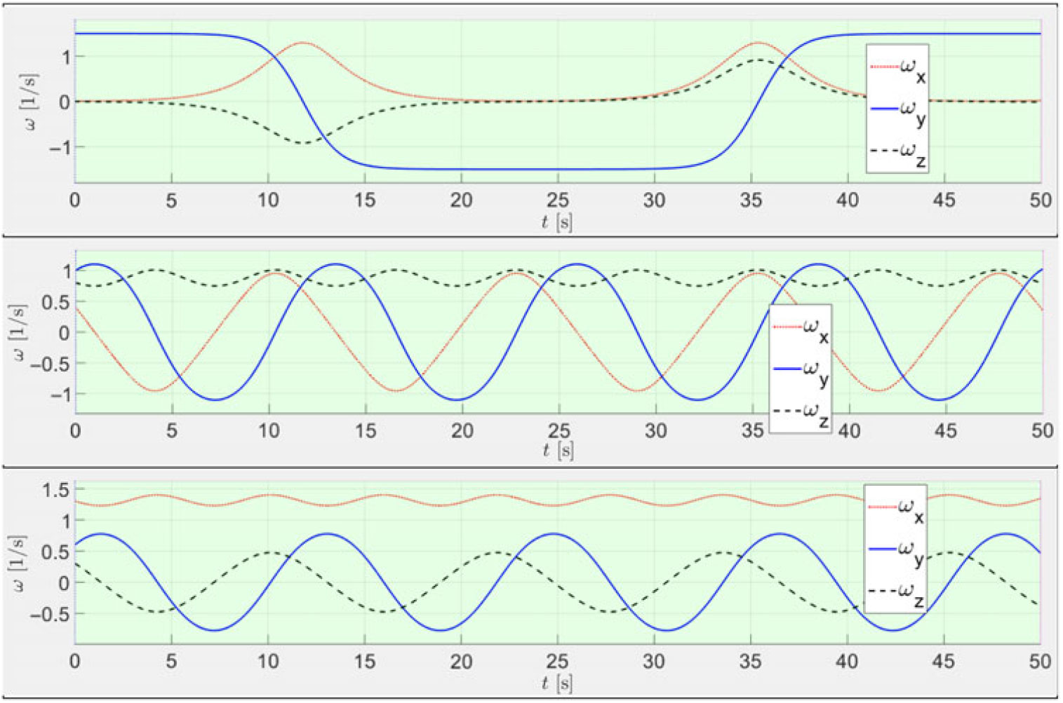
For illustration purposes, we solve Euler’s Eqs. (1) for the same system with I_xx = 2; I_yy = 3; I_zz = 4 [all in kg×m²], which corresponds to ξ = 0.5 and η = 0.5, but consider three contrast cases of the initial conditions. An example of the results of the numerical simulations for ω_x, ω_y, ω_z are shown in Fig. 1.

Figure 1. Time histories for angular velocity components ω_x, ω_y, ω_z for three contrast cases of initial conditions: (A) ω _x0 = 0.01, ω _y0 = 1.5, ω _z0 = 0.01; (B) ω _x0 = 0.4, ω _y0 = 1, ω _z0 = 0.8; (C) ω _x0 = 1.3, ω _y0 = 0.6, ω _z0 = 0.3 (here and further all angular velocities are given in rad/s).

For the more general interpretation, the introduction of non-dimensional angular momentum coordinates is proposed:

(5)\begin{align}{{{\overline H}_x}(t)= {H_x}/{H_0} = {I_{xx}}{\omega_x}/\sqrt {{{\left( {{I_{xx}}{\omega_x}} \right)}^2} + {{\left( {{I_{yy}}{\omega_y}} \right)}^2} + {{\left( {{I_{zz}}{\omega_z}} \right)}^2}}\nonumber\\ {{\overline H}_y}(t) = {H_y}/{H_0} = {I_{yy}}{\omega_y}/\sqrt {{{\left( {{I_{xx}}{\omega_x}} \right)}^2} + {{\left( {{I_{yy}}{\omega_y}} \right)}^2} + {{\left( {{I_{zz}}{\omega_z}} \right)}^2}}\\\nonumber{{\overline H}_z}(t) = {H_z}/{H_0} = {I_{zz}}{\omega_z}/\sqrt {{{\left( {{I_{xx}}{\omega_x}} \right)}^2} + {{\left( {{I_{yy}}{\omega_y}} \right)}^2} + {{\left( {{I_{zz}}{\omega_z}} \right)}^2}}}\end{align}

where H₀ is the initial value of the angular momentum of the system, and H_x, H_y, and H_z are its components in the body axes system x, y and z. Non-dimensional coordinates ${\skew3\overline H_x},\;{\skew3\overline H_y},\;{\skew3\overline H_z}$ enable us to express the law of conservation of the angular momentum in the compact form

(6)\begin{equation}{\skew3\overline H_x}^2 + {\skew3\overline H_y}^2 + {\skew3\overline H_z}^2 = 1\end{equation}

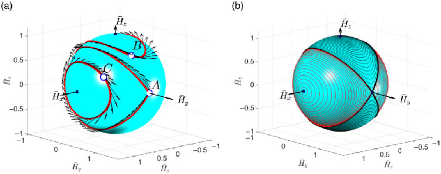
Equation (6) can be conveniently interpreted as a unit sphere, known as the angular momentum sphere, AMS. This concept will be consistently used in this paper to illustrate simulation results. For example, Fig. 2 provides with an alternative interpretation of the previous cases A, B and C with polhodes^{(Reference Wie7)} — trajectories of the tips of the non-dimensional angular momentum vectors, ${\overline {\bf{H}}_A}$, ${\overline {\bf{H}}_B}$ and ${\overline {\bf{H}}_C}$ (these three polhodes are marked with the red color), residing on the AMS. Figure 2 also shows three superimposed quiver plots for these ${\overline {\bf{H}}_A}$, ${\overline {\bf{H}}_B}$ and ${\overline {\bf{H}}_C}$ vectors.

Figure 2. Polhodes: (a) for demonstration cases A, B and C in Fig. 1; (b) examples of broad coverage of initial conditions.

4.0 POLHODES AND SEPARATRICES

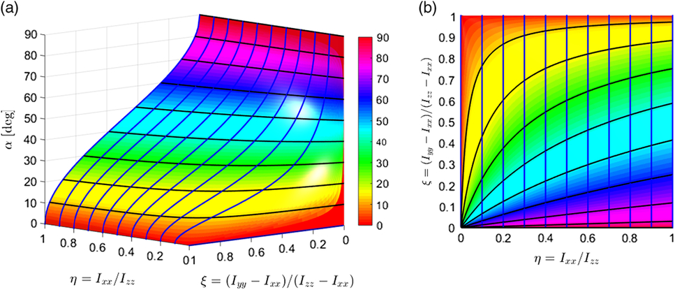
Figure 2b shows that the polhodes can be split into four groups, separated by the (shown as bold black) lines, called separatrices. In case of I_yy being the intermediate moment of inertia, two separatrices intersect at the points on the y axis. It is possible to show that polhodes are seen on orthogonal projections as ellipses, hyperbolas and ellipses, and separatrices are seen on the x-z projection as two lines, passing through the y axis, reduced on projection to a dot point. We can calculate an important characteristic of the rotational motion of the spacecraft, α - angle of inclination of the separatrix plane with respect to the z axis^{(Reference Trivailo and Kojima3)}:

(7)\begin{align}\quad \quad \alpha = \arctan \left( {\sqrt {{{{\mkern 1mu} {\mkern 1mu} {I_x}{\mkern 1mu} {\mkern 1mu} ({I_y} - {I_z})} \over {{I_z}{\mkern 1mu} {\mkern 1mu} ({I_x} - {I_y})}}} } \right) = \arctan \left( {\sqrt {{\mkern 1mu} {\mkern 1mu} \eta {\mkern 1mu} {\mkern 1mu} {\mkern 1mu} {\mkern 1mu} \left( {{1 \over \xi } - 1} \right)} } \right) \\({\rm{only\ applicable\ for\ the\ }}{I_{xx}} \lt {I_{yy}} \lt {I_{zz}}{\rm{\,notations\ and\ }}0 \lt \eta \lt 1{\rm{\ and\ }}0 \lt \xi \lt 1)\nonumber \end{align}

Changes in the angle α due to the variation in both, η and ξ, are shown in Fig. 3. Note, that for convenience, values of α angles are presented in degrees.

Figure 3. Changes in the angle α due to the variation in both, η and ξ: (a) 3D surface plot for α(η,ξ) function with colorbar added; (b) 2D projection of the α(η,ξ) surface with its contour lines: η = 0: 0.1: 1; α = 0: 10: 90.

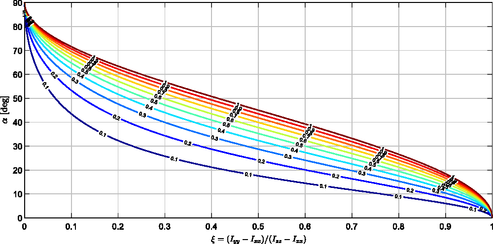
The method, described in^{(Reference Trivailo and Kojima3)}, was based on the calculation of the value of the intermediate moment of inertia I_yy for the specified angle α and known values of I_xx = 2.4 and I_zz = 3.15. For this formulation, Eq. (7) can be re-written as follows:

(8)\begin{equation}\xi = {\left\{ {1 + \left[ {{{(\tan \alpha )}^2}/\eta } \right]} \right\}^{ - 1}}\end{equation}

In the particular case considered in reference^{(Reference Trivailo and Kojima4)}, for I_xx = 2.4 and I_zz = 3.15, the corresponding value of η is equal to η = 0.7619; furthermore, Eq. (8) gives ξ = 0.5907, which (as per Eq. (3)), corresponds to I_xx = 2.8430.

The generic graphical method, corresponding to this procedure, is illustrated in Fig. 4, where angle α (shown in degrees) is plotted as a function of ξ for various values of η = [.1, .2, .3, .4, .5, .6, .7, .8, .9, 1].

Figure 4. Changes in the angle α due to the variation in ξ for selected values of η = [1:10]/10.

5.0 KINETIC ENERGY ELLIPSOID AND GEOMETRIC INTERPRETATION OF POLHODES

The kinetic energy of the rotating body can be expressed in terms of the angular momentum components, such as follows:

(9)\begin{equation}\frac{1}{2}{I_{xx}}\omega_x^2 + \frac{1}{2}{I_{yy}}\omega_y^2 + \frac{1}{2}{I_{zz}}\omega_z^2 = {\left[ {\frac{{{H_x}(t)}}{{\sqrt {2{I_{xx}}} }}} \right]^2} + {\left[ {\frac{{{H_y}(t)}}{{\sqrt {2{I_{yy}}} }}} \right]^2} + {\left[ {\frac{{{H_z}(t)}}{{\sqrt {2{I_{zz}}} }}} \right]^2} = K(t)\end{equation}

In the context of the inertial morphing concept (presented later in the paper), it’s essential to consider the general case allowing for the principal moments of inertia of the system to change with time:

(10)\begin{equation}{\left[ {\frac{{{H_x}(t)}}{{\sqrt {2{I_{xx}}(t)} }}} \right]^2} + {\left[ {\frac{{{H_y}(t)}}{{\sqrt {2{I_{yy}}(t)} }}} \right]^2} + {\left[ {\frac{{{H_z}(t)}}{{\sqrt {2{I_{zz}}(t)} }}} \right]^2} = K(t)\end{equation}

Being dedicated to the non-dimensional formulation, we divide both sides of this equation by the constant ${H_0}^2$ and rearrange result in terms of non-dimensional quantities ${\skew3\overline H_x}$, ${\skew3\overline H_y}$ and ${\skew3\overline H_z}$:

(11)\begin{equation}{\left[ {\frac{{{H_x}(t)}}{{{H_0}}}\;\frac{1}{{\sqrt {2{I_{xx}}(t)} }}} \right]^2} + {\left[ {\frac{{{H_y}(t)}}{{{H_0}}}\;\frac{1}{{\sqrt {2{I_{yy}}(t)} }}} \right]^2} + {\mkern 1mu} {\mkern 1mu} {\mkern 1mu} {\mkern 1mu} {\left[ {\frac{{{H_z}(t)}}{{{H_0}}}\;\frac{1}{{\sqrt {2{I_{zz}}(t)} }}} \right]^2} = \frac{{K(t)}}{{{{[{H_0}]}^2}}}\end{equation}

In view of Eqs. (6), this equation can be rewritten in terms of the non-dimensional angular momentum components:

(12)\begin{equation}{\left[ {\frac{{{{\skew3\overline H}_x}}}{{\sqrt {2{I_{xx}}(t)} }}} \right]^2} + {\left[ {\frac{{{{\skew3\overline H}_y}}}{{\sqrt {2{I_{yy}}(t)} }}} \right]^2} + {\mkern 1mu} {\mkern 1mu} {\mkern 1mu} {\left[ {\frac{{{{\skew3\overline H}_z}}}{{\sqrt {2{I_{zz}}(t)} }}} \right]^2} = \frac{{K(t)}}{{{{[{H_0}]}^2}}}\end{equation}

Finally, Eq. (12), can be written in its useful final form, used in this paper, as follows:

(13)\begin{equation}{\left[ {\frac{{{{\skew3\overline H}_x}}}{{\displaystyle\frac{{\sqrt {2{\mkern 1mu} K(t){\mkern 1mu} \;{I_{xx}}(t)} }}{{{H_0}}}}}} \right]^2} + {\left[ {\frac{{{{\skew3\overline H}_y}}}{{\displaystyle\frac{{\sqrt {2{\mkern 1mu} K(t){\mkern 1mu} \;{I_{yy}}(t)} }}{{{H_0}}}}}} \right]^2} + {\mkern 1mu} {\mkern 1mu} {\mkern 1mu} {\mkern 1mu} {\left[ {\frac{{{{\skew3\overline H}_z}}}{{\displaystyle\frac{{\sqrt {2{\mkern 1mu} K(t){\mkern 1mu} \;{I_{zz}}(t)} }}{{{H_0}}}}}} \right]^2} = 1\end{equation}

Equation (13) corresponds to the so called kinetic energy ellipsoid (KES) in the ${\skew3\overline H_x}$, ${\skew3\overline H_y}$ and ${\skew3\overline H_z}$ axis, with the following values of the semi-major axes:

(14)\begin{equation}{a_x} = \frac{{\sqrt {{\mkern 1mu} 2{\mkern 1mu} K(t){\mkern 1mu} {\mkern 1mu} {\mkern 1mu} {\mkern 1mu} {I_{xx}}(t)} }}{{{H_0}}};\quad {a_y} = \frac{{\sqrt {{\mkern 1mu} 2{\mkern 1mu} K(t){\mkern 1mu} {\mkern 1mu} {\mkern 1mu} {I_{yy}}(t)} }}{{{H_0}}};\quad {a_z} = \frac{{\sqrt {{\mkern 1mu} 2{\mkern 1mu} K(t){\mkern 1mu} {\mkern 1mu} {\mkern 1mu} {I_{zz}}(t)} }}{{{H_0}}}\end{equation}

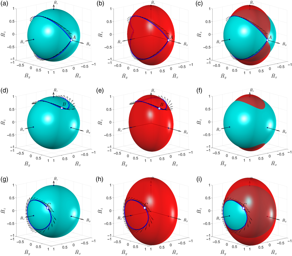
In addition to the angular momentum spheres with specific polhodes for the cases A, B and C (Fig. 5, left column), let us also plot corresponding kinetic energies ellipsoids (Fig. 5, middle column). Then, combining the surfaces in these two columns, we can see that specific polhodes are, in fact, lines of intersection between corresponding AMSs and KEEs (Fig. 5, right column).

Figure 5. (a),(d),(g) Angular momentum unit spheres (left column); (b),(e),(h) kinetic energy ellipsoids (middle column) for Cases-A,B,C; (c),(f),(i) Superimposed AMSs and KEEs.

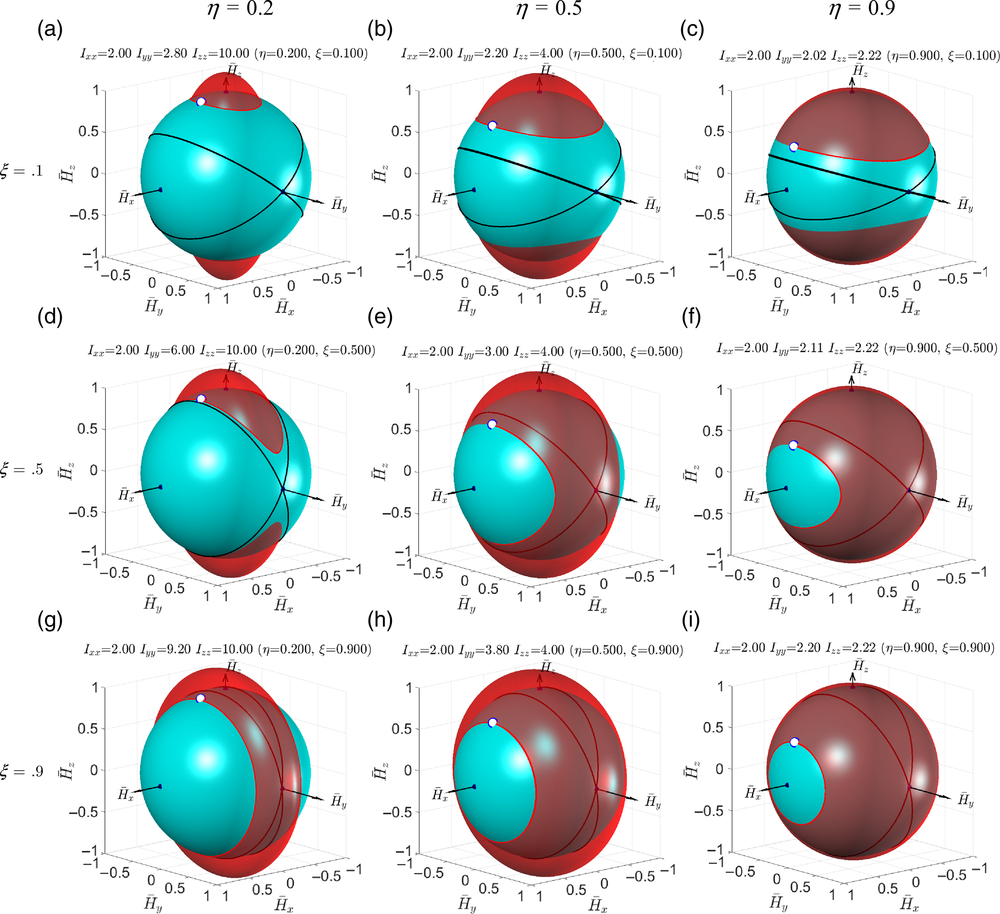
Utilising conveniences of the non-dimensional notations, we can illustrate influence of the variables ξ and η on the shapes of the kinetic energy ellipsoids and polhodes. Figure 6 presents nine contrast cases for the combinations of ξ = [0.1, 0.5, 0.9] and η = [0.2, 0.5, 0.9].

Figure 6. Contrast cases of simulations of the rotating rigid body with the same initial conditions (ω _x0 = 1; ω _y0 = 0; ω _z0 = 1.5 - all in rad/s) and I_xx = 2kg × m², illustrating changes of the shape of the kinetic energy ellipsoid due to the changes in η and ξ.

6.0 THE DZHANIBEKOV’S EFFECT AND TENNIS RACQUET THEOREM

The motion of the spinning rigid body, labelled as Case-A, has a very special significance, as it is related to the so called Dzhanibekov’s Effect and Tennis Racquet Theorem^{(Reference Murakami, Rios and Impelluso6)}. Let us present a brief history of this intriguing phenomenon, partially reproduced from the reference^{(Reference Trivailo and Kojima4)}.

Vladimir Aleksandrovich Dzhanibekov (see Fig. 7a) is one of the USSR’s famous cosmonauts. During his fifth space flight, on June 25, 1985, he discovered a spectacular phenomenon: a spinning wing nut in its stable flight suddenly changed its orientation by 180 degrees and continued its flight backwards, simultaneously changing its direction of rotation to opposite! (It should be noted that wing nuts, shown in Fig. 7a and 8a, are widely used in space for fixing payloads: their shape enables removal of the wingnuts without special tools.)

Figure 7. (a) Vladimir A. Dzhanibekov, Interview at the “Secret Signs” TV Program, explaining flipping of the wing nut, https://youtu.be/dL6Pt1O_gSE (accessed 12/10/2019); (b) Owen K. Garriott, (1973), Demonstration on board of Skylab 3 of the flipping object, spun about its intermediate axis, https://youtu.be/xdtqVR1CgQg?t=1018 (accessed 19/02/2019).

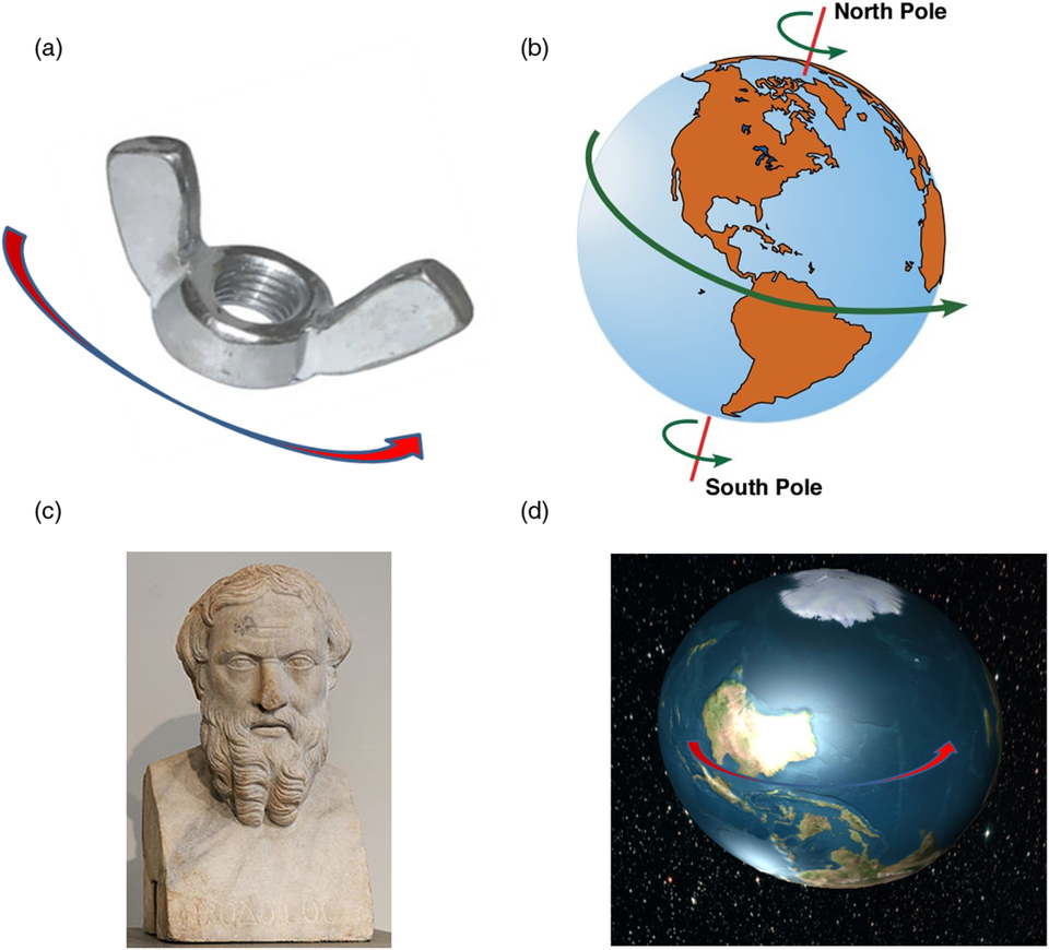
Figure 8. Is our planet, Earth, flipping similar to the wingnut? (a) simple wingnut; (b) planet Earth; (c)Herodotes, famous Greek historian; (d) imagined “flipped” Earth.

Dzhanibekov realised that this pattern of motion repeated itself in the periodic sequence. Similar experiments have subsequently been run on-board of the International Space Station. Observing these experiments in space, it could be clearly seen that the spinning object always rotates in the same direction relative to the observation camera (fixed to the inertial coordinates frame): that means that in the reference frame of the rotating handle the direction of rotation flips each time its orientation flips.

Performing detailed literature search, we were able to find even earlier demonstrations in space of the flipping motion of the spinning rigid body, dated in 1973. Figure 7b shows a snapshot from the space experiment video, where famous U.S. scientist-astronaut Owen Kay Garriott is performing a dynamics experiment onboard Skylab-3. On the snapshot, he is initiating a spin of the rigid body in zero gravity by providing an energetic torque impulse about the intermediate axis of inertia of the body, which instantly results in the peculiar rotational motion of the boxed object about this axis with clearly observed periodic flipping about this axis. Therefore, it has been documented, that the so called Dzhanibekov’s Effect was observed in space in 1973 by Owen Garriott, twelve years before the same phenomenon was also observed in space in 1985 by Vladimir Dzhanibekov, whose name was given to the phenomenon.

Surprisingly, the flipping motion phenomenon, which initially was perceived by some as counter-intuitive was conceptually predicted in 1971 by Beachley^{(Reference Beachley9)}, however this work for very long time has been left unnoticed and popular, in-depth explanation of the phenomenon has only been very recently presented in the journal publication^{(Reference Murakami, Rios and Impelluso6)}. The Dzhanibekov’s Effect has been closely linked to the peculiar behaviour and explanation of the flipped tennis racket, which has received special names, such as Tennis Racket Theorem and intermediate axis theorem.

Explanation of both, Dzhanibekov’s Effect and Tennis Racket Theorem is based on the great Euler equations, published in their canonical form in 1758^{(Reference Trivailo and Kojima5)}.

Interestingly, Euler’s equations paved the theoretical ground to many scientific manifestations, including Coriolis forces, predicted by Euler, but interpreted to the world many years later by French scientist Gaspard-Gustave de Coriolis in 1835.

Entrancingly, that promotion of the Dzhanibekov’s Effect has prompted development of the theories, suggesting that our planet, Earth, is performing periodic flips, similar to the wing nut (see Fig. 8d). Some researchers in the media has suggested that our planet, Earth, having much more substantial properties (I ∼ 8 × 10³⁷ kg·m²), is performing these flips with much higher period, estimated to be at the order of 12,000 years. There were even some substantiation presented to justify this statement: firstly, periodicity in the changes in the magnetic field of the Earth; secondly, reference to the ancient Greeks historian, Herodotus (lived in the fifth century BC, c. 484–c. 425 BC, see Fig. 8c); and thirdly, references to the religious texts. For example, reference⁽¹⁰⁾ states: “Herodotus wrote that Egyptian priests had told him that four times since Egypt became a kingdom the Sun rose contrary to his wont; twice he rose where he now sets, and twice he set where he now rises.” The Egyptians had a name for the Sun when it rose in the west, Re-Horakhty. And the concept of the Sun rising in the west occurs in both Christian and Muslim literature. There were also accounts of stars reversing the direction of rising, while various texts talk of north becoming south at a time of chaos. This reversal also appears in Greek literature, most notably in the Statesman of Plato.

The hypothesis of the flipping Earth, despite of being very intriguing, is full of controversy (for example, under conventional assumptions, the Earth is not rotating about its intermediate axis, etc.), and is not pursued further in this paper.

7.0 DEMONSTRATIONS OF THE DZHANIBEKOV’S EFFECT ON BOARD OF THE ISS

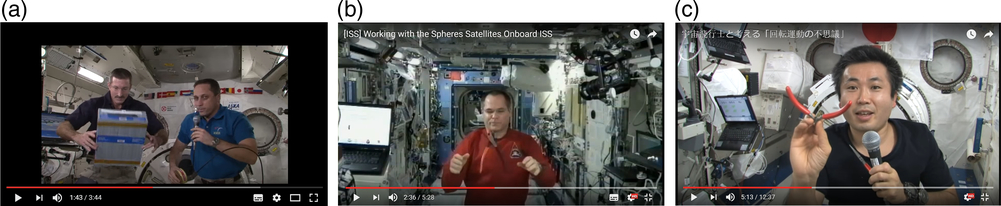
Due to its simplicity and intriguing nature, the Dzhanibekov’s Effect has been became one of the most popular educational and scientific experiments on board of the ISS. It has been reproduced with various rigid body objects and even liquids. Various videos on these experiments, available in the media, are excellent educational resources. For example, influence of the shape of the rigid bodies, thus mass distribution in various rigid bodies, including cylinders, cubes and right rectangular prisms, was demonstrated on board of the ISS by Dan Burbank and Anton Shkaplerov (see Fig. 9a), members of thethirtieth expedition^{(Reference Shkaplerov and Burbank11)}.

Figure 9. Demonstrations of the Dzhanibekov’s Effect onboard the ISS.

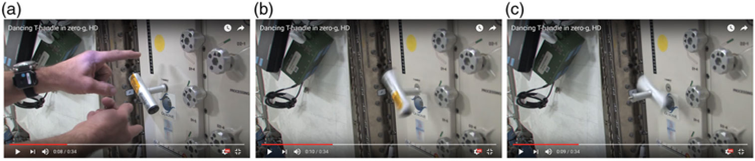
Figure 10. Dancing T-handle in zero gravity.

American astronaut Kevin Ford (NASA), (thirty-fourth expedition)^{(Reference Wakata12)} (see Fig. 9b) and Japanese astronaut Koichi Wakata (JAXA), (thirty-eighth expedition)^{(Reference Ford13)} (see Fig. 9c) experimented onboard the ISS with nothing more complex that pliers. They used this adjustable geometry tool as an object, capable of intriguing spinning, flipping and tumbling in zero gravity.

One of the most fascinating movies is a continuous short-period flipping of the T-handle onboard the ISS, fairly called as dancing T-handle^{(Reference Kawano14)} (see Fig. 10). This is a wonderful demonstration of the Dzhanibekov’s Effect, which very convincingly illustrates instability of rotation of the rigid body with distinct principal moments of inertia, if the main spin is provided about its principal axis, associated with intermediate moment of inertia.

All these and other demonstrations can be explained by Euler equations. Of course, this is of great interest to be able to explain interesting phenomenon of the flipping spinning systems, however, we noticed new opportunities of controlling these peculiar motions and proposed a method of control, based on the inertial morphing, involving changes of the principal moments of inertia of the system. This concept will be explained later on in the paper. However, before this, let us discuss the calculation of the period of the flipping motions in the Dzhanibekov’s Effect and Tennis Racquet Theorem demos. We present some interesting results and a relevant extract from our work^{(Reference Trivailo and Kojima4)}.

8.0 CALCULATION OF THE PERIOD OF THE FLIPPING MOTION

As stated earlier, we assume that I_yy is intermediate value of the principal moment of inertia. Then the period of the observed unstable motion can be estimated, using Eq. (37.12) on page 154 from the L.D.Landau reference^{(Reference Landau and Lifshitz15)}:

(15)\begin{equation}{\rm {If}} {\,\,H^2} \gt 2{K_0}{\mkern 1mu} {\mkern 1mu} {I_{yy}},\end{equation}

which is equivalent to a_y < 1 (see Eq. 14), then

(16)\begin{equation}T = 4K{\mkern 1mu} \sqrt {\frac{{{I_{xx}}{\mkern 1mu} {I_{yy}}{\mkern 1mu} {I_{zz}}}}{{({I_{zz}} - {I_{yy}}){\mkern 1mu} ({H^2} - 2{K_0}{\mkern 1mu} {I_{xx}})}}}\end{equation}

(17)\begin{equation}{\rm {If}} {\,\,H^2} \lt 2{K_0}{\mkern 1mu} {\mkern 1mu} {I_{yy}},\end{equation}

which is equivalent to a_y > 1 (see Eq. 14), then

(18)\begin{equation}T = 4K{\mkern 1mu} \sqrt {\frac{{{I_{xx}}{\mkern 1mu} {I_{yy}}{\mkern 1mu} {I_{zz}}}}{{({I_{xx}} - {I_{yy}}){\mkern 1mu} ({H^2} - 2{K_0}{\mkern 1mu} {I_{zz}})}}}\end{equation}

where K is complete elliptic integral of the first kind:

(19)\begin{equation}K = \int\limits_0^1 {\frac{{ds}}{{\sqrt {\left( {1 - {s^2}} \right)\left( {1 - {k^2}{s^2}} \right)} }}} = \int\limits_0^{\pi /2} {\frac{{du}}{{\sqrt {1 - {k^2}{\mkern 1mu} {{\sin }^2}u} }}} \end{equation}

As an illustrative example, let us assume the following parameters of the system: I_xx = 3, I_zz = 3.5 (all in kg×m²), with the initial conditions _iω _x = 0.1, _iω _y = 15, _iω _z = 0.1 (all in rad/s). For this case we will use equations (15)–(19) and will illustrate the influence of the intermediate moment of inertia I_yy of the system on the period of the unstable flipping motion. The resulting plot, presented in Fig. 11, is clearly being asymmetrical, could be easily regarded by many as counter-intuitive, as there may be a wrongly perceived assumption of the “symmetrical” influence of I_yy on period T.

Figure 11. Period of the unstable flipping motion (Dzhanibekov’s Effect case) of the rigid body, as a function of its intermediate moment of inertia I_yy for the following example: I_xx = 3; I_zz = 3.5[kg × m²]; ω _x0 = 0.1, ω _y0 = 15, ω _z0 = 0.1[rad/s].

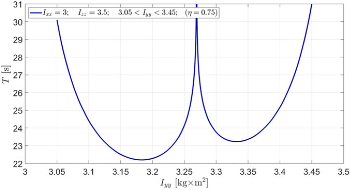
The plot in Fig. 11 prompts that when I_yy is approaching any of the other moments of inertia, I_xx or I_zz, then the period of the flipping is asymptotically approaching infinite values. Also, this plot prompts that variation in the intermediate value of the moment of inertia between I_xx and I_zz (i.e. changing the ξ value) can allow changes of the period T of the flipping motion within wide range. However, there is a minimum value of the period, which could not be reduced further. For the example shown, the lower threshold of the period is slightly higher than 22.2 seconds. Also, there is a specific value of the I_yy that leads to the infinitely large value of the T. For the example shown, this corresponding value of I_yy is approximately 3.27kg×m².

Similarly to the example above, in the second illustrative example, we initially assume initial conditions ω _x0 = 0.01, ω _y0 = 1.5, ω _z0 = 0.01 (all in rad/s) for the system with I_xx = 2, I_zz = 4 (all in kg×m²), which corresponds to η = 0.5 (see Eq. 2) and plot the flipping period as a function of the intermediate moment of inertia I_yy, varying its value in-between the minimum value of the moment of inertia I_xx and maximum value of the moment of inertia I_zz. The resultant plot is shown in Fig. 12a with a continuous red line. It allows determination of the flipping period for the Case A, illustrated previously in Figs. 1a, 2a, 5a,5b, and 5c. This value is equal to 47.16s, which is in agreement with Fig. 1a. Let us now, in addition to the above, consider a similar “variable I_yy” experiment, changing only the maximum moment of inertia value from I_zz = 4 to I_zz = 5, which would correspond to η = 0.4. The resultant plot for the period is shown with dotted blue line in Fig. 12a. Comparison of the two curves allows to suggest another avenue for manipulation with the period of the flipping motion by changing the ratio between I_xx and I_zz, i.e. η value.

Figure 12. Period of the unstable flipping motion (Dzhanibekov’s Effect case) of the rigid body, as a function of its moments of inertia I_yy and I_zz for two variation experiments: (a) variation of I_yy only in two cases I_xx = 2; I_zz = 4; and I_xx = 2; I_zz = 4[kg × m²]; ω _x0 = 0.01, ω _y0 = 1.5, ω _z0 = 0.01[rad/s]; (b) variation of both, I_yy and I_zz in the case I_xx = 2[kg × m²]; ω _x0 = 0.01, ω _y0 = 1.5, ω _z0 = 0.01[rad/s].

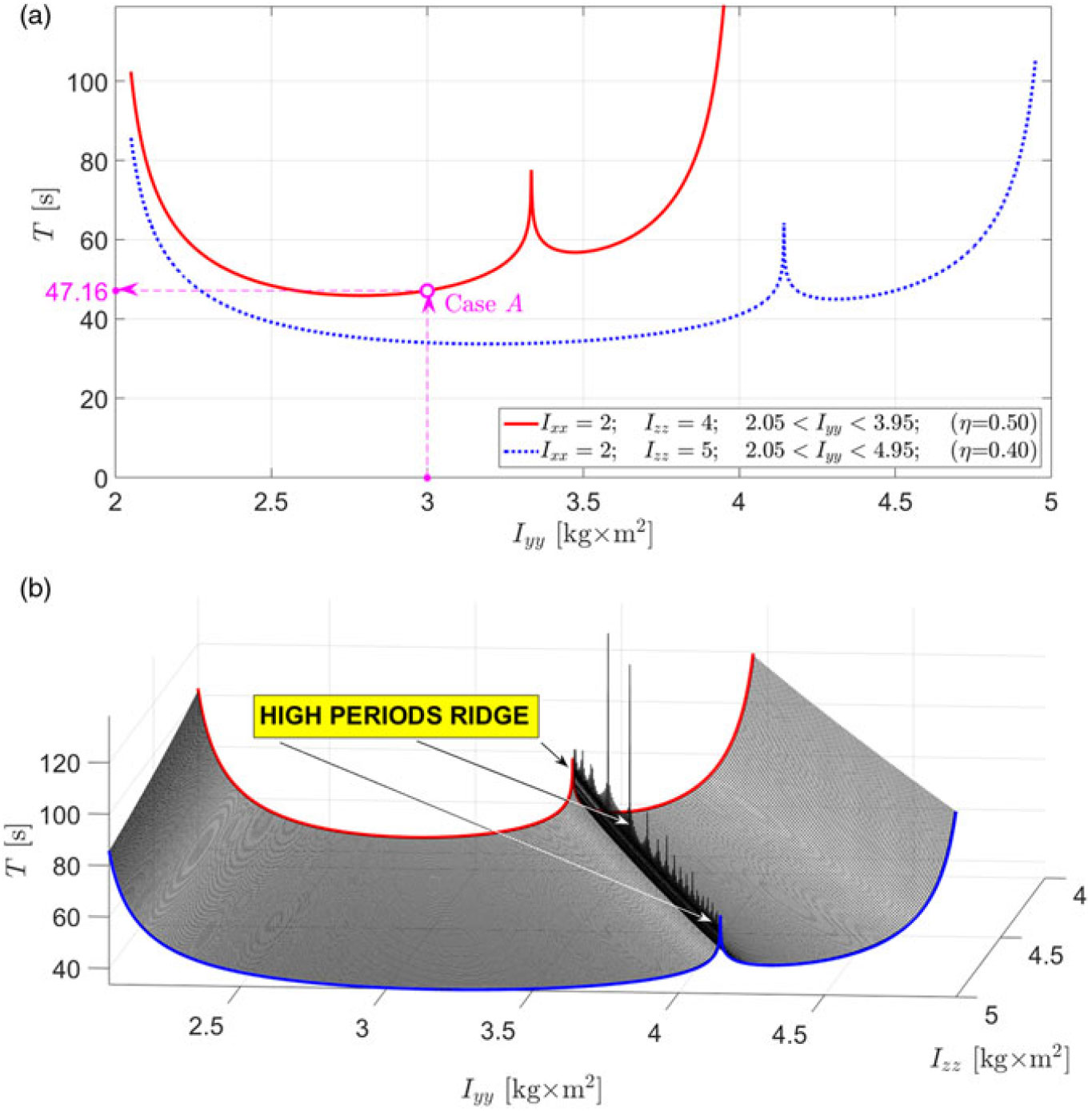
Allowing variation of the I_yy and I_zz values (i.e. ξ and η non-dimensional parameters), we can also calculate more generic plot, showing influence of these principal moments of inertia on the period T of the unstable motion. The resultant plot is shown in Fig. 12b. This is an interesting plot, which shows more generic nature of the asymmetry, observed in Fig. 11 and Fig. 12a. Figure 12b comprises the two curves (red and blue), presented in Fig. 12a. However, most significant observation in Fig. 12b is that for each of the I_zz values, there is a value of I_yy which leads to the infinitely large period of the flipping motion. We named this area as “high periods ridge”, clearly labelled in Fig. 12b.

9.0 CONCEPT OF THE INERTIAL MORPHING OF THE SPACECRAFT

As an enhancement in the control capabilities of the spacecraft, in our previous works^{(Reference Trivailo and Kojima1–Reference Trivailo and Kojima5)}, we proposed a concept of inertial morphing: we showed that using special devices (with, for example moving masses) or other means and/or phenomena, (for example, moving liquids, mass evaporation, solidification, ablation), enabling controlled modifications of the principle moments of inertia characteristics, the attitude dynamics of the spacecraft could be efficiently controlled.

Assume that the spacecraft has morphing capabilities, allowing independent controllable changes of the values of the principal moments of inertia. A basic model of the morphing spacecraft, involving three orthogonal dumbbells, each of which has negligible mass of the rod, connecting two equal concentrated masses at its ends, was considered in^{(Reference Trivailo and Kojima5)} and is reproduced in Fig. 13.

Figure 13. Six-mass conceptual model of the morphing spacecraft.

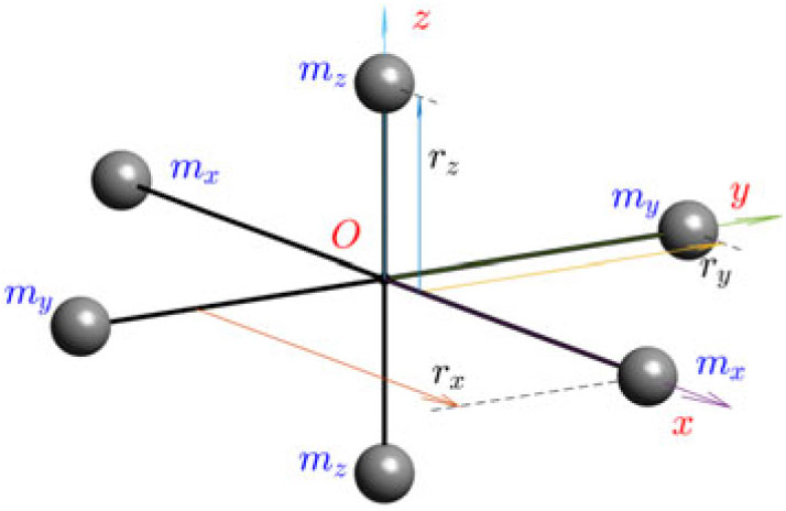
Let us also assume, for conceptual simplicity, that three dumbbells are connected at the middle points of their rods, and the corresponding masses m_x, m_y and m_z are located at the distances r_x, r_y and r_z from the axes of rotation x, y and z, as shown in Fig. 13. In the illustrated conceptual design, morphing of the spacecraft is achieved via independent synchronized control of the position coordinates r_x = r_x(t), r_y = r_y(t) and r_z = r_z(t) of the masses m_x, m_y and m_z.

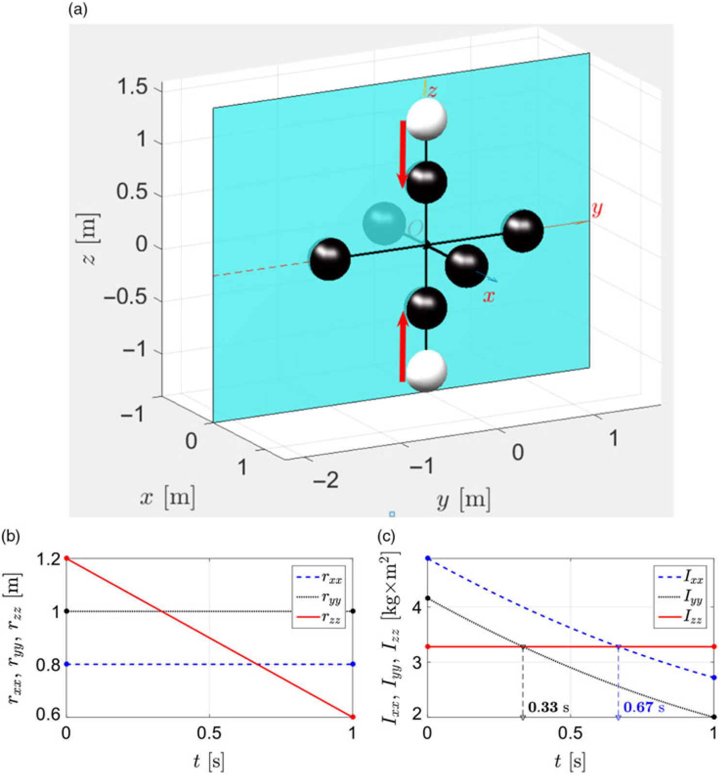
Figure 14. Particular example of inertial morphing via translational re-position of the z dumbbell masses m_z, while keeping positions of the x and y masses unchanged (m_x = m_y = m_z = 1kg): (a) 3D view of the spacecraft model; (b) time history of the position of the masses; (c) time history of the resulting principal moments of inertia I_xx, I_yy and I_zz.

Indeed, changing the distance between three pairs of the masses could be used to achieve any values of the principal moments of inertia I_xx, I_yy and I_zz. To achieve this objective, it would be sufficient to move masses to the following radii:

(20)\begin{equation}{r_x} = \sqrt {\frac{{{\mkern 1mu} {\mkern 1mu} {I_{yy}} + {I_{zz}} - {I_{xx}}}}{{4{\mkern 1mu} {\mkern 1mu} {m_x}}};} \quad {r_y} = \sqrt {\frac{{{\mkern 1mu} {\mkern 1mu} {I_{zz}} + {I_{xx}} - {I_{yy}}}}{{4{\mkern 1mu} {\mkern 1mu} {m_y}}};} \quad {r_z} = \sqrt {\frac{{{\mkern 1mu} {\mkern 1mu} {I_{xx}} + {I_{yy}} - {I_{zz}}}}{{4{\mkern 1mu} {\mkern 1mu} {m_z}}}}\end{equation}

These important relationships can be easily obtained from the equations for principal moments of inertia of the system^{(Reference Curtis16)}:

(21)\begin{equation}{I_{xx}} = 2{\mkern 1mu} {\mkern 1mu} {m_y}{\mkern 1mu} r_y^2 + 2{\mkern 1mu} {\mkern 1mu} {m_z}{\mkern 1mu} r_z^2;\quad {I_{yy}} = 2{\mkern 1mu} {\mkern 1mu} {m_z}{\mkern 1mu} r_z^2 + 2{\mkern 1mu} {\mkern 1mu} {m_x}{\mkern 1mu} r_x^2;\quad {I_{zz}} = 2{\mkern 1mu} {\mkern 1mu} {m_x}{\mkern 1mu} r_x^2 + 2{\mkern 1mu} {\mkern 1mu} {m_y}{\mkern 1mu} r_y^2\end{equation}

10.0 SUGGESTIONS ON SOME PRACTICAL IMPLEMENTATION OF THE INERTIAL MORPHING

This paper does not aim to present comprehensive collection of the implementation of the methods to control the principal moments of inertia of the spacecraft, we called “inertial morphing”. Nevertheless, for completeness, we wish to present just a few of the methods/concepts, being considered as promising for realization in real spacecraft systems. In these examples, for simplicity of the illustrations, the conceptual model of the spacecraft (Fig. 13) will be used. As equations for the moments of inertia are functions of the distances r and masses m, conceptually, there could be two main approaches to the implementation of the inertial morphing: (a) based on variation of r - positions of the masses and (b) based on variation of masses. These approaches are briefly explained below.

1. (a) The first approach to implementation of the inertial morphing is based on the controlled re-position of the spacecraft masses, using actuators. Let us consider the following case: m_x = m_y = m_z = 1kg; these masses are initially located at their radii: r_x = 0.8m; r_y = 1m; r_z = 1.2m. Let us assume that the system is equipped with linear actuator (motor and appropriate mechanical system), capable of translational re-positioning of the masses m_z via changing the length of r_z from 1.2m to 0.6m within 1s. The morphing process is shown in Fig. 14a, where initial positions of the masses are shown with white spheres, and the final positions — with black spheres and where direction of the translations for two m_z masses is shown with two red arrows. Also, for better perception of the 3D design, a semi-transparent yz plane is added to Fig. 14a.

In this example, the positions of the masses on the x and y axes remain unchanged, only r_z is subject to variation (as per Fig. 14b). Equation. (21) permits the calculation of the associated resulting time history of the principle moments of inertia of the system. Figure 14c shows that while I_xx keeps its value unchanged, during morphing, the I_xx value is changing from 4.88 to 2.72 [kg×m²] and the I_xx is changing from 4.16 to 2.0 [kg×m²]. However, most significant in the context of this paper is an observation that, in this example, the role of the intermediate moment of inertia (which initially “belongs” to I_yy) is “passed” from I_yy to I_zz (at t = 0.33s) and then is further passed to I_xx (at t = 0.67s). Consequently, using only one variable r_z in the morphing process, it was possible to arrange for each of the spacecraft axes x, y and z at different stages, to become the intermediate axis of rotation.

The method presented above can be extended to the actuation of all masses, including m_x and m_y. With this general arrangement, the morphing would permit continuous control of the position of all masses, hence, would enable assignment of any arbitrary values to the principal moments of inertia of the system, as per requirements of the morphing scenarios. Of course, these assignments should be compatible with the mechanical/electrical/thermal constrains of the particular designs/implementations of the morphing systems.

A variation of the same method may involve application of the special actuators to re-position large segments of the spacecraft. This idea is illustrated with the controlled change of the angular positions θ_i of the solar panels to manipulate the inertial properties of the spacecraft (see Fig. 15).

Figure 15. Spacecraft, deploying solar arrays^{(Reference Yao and Ge17)}.

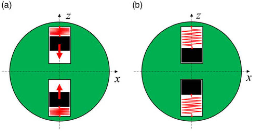
We envisage that similar implementations of the illustrated principle can be achieved in some other ways. For example, deployment of the masses, to the new destination (in any, inwards, outwards or inclined directions) can be ensured via un-constraining the pre-compressed springs, as per Fig. 16. This, however, would permit only a single discrete actuation.

Figure 16. Particular example of inertial morphing via translational re-position of the z dumbbell masses m_z, (shown with black color) via release of the pre-constrained compressed springs (shown with red color): (a) initial configuration; (b) masses deployed inwards.

Alternatively, for continuous actuation, instead of using solid masses, heavy liquids and/or liquid metals ^{(Reference Noack18)} can be used, which could be controlled via manipulation with valves and employment of the passive inertial forces and/or controlled magnetic field forces to move these liquid medias.

1. (b) The second approach to implementation of the inertial morphing is based on the controlled change of the spacecraft masses and may involve, for example, mass ejection; ablation, evaporation or solidification of the components of the structure, etc.

Geometric reconfigurations of the spacecraft systems (for example, during deployment of the inflatable components or solar panels, and reorientation of the antennae) is a widely used concept and proved to be successful for many space systems (for example, Spartan-207, Hughes/Boeing HS-376, SMART-1 and RAE-B satellites, space probes Rosetta and Down, etc.). However, these are provided to ensure the functionality of the spacecraft, without any relevance to the attitude dynamics objectives^{(Reference Hwang, Lee, Cutler and Martins19)}. In contrast, concept of spacecraft reconfiguration, explicitly aiming to assist in attitude maneuvering^{(Reference Trivailo and Kojima1–Reference Trivailo and Kojima5)}, is a very new concept. Indeed, idea of the reconfigurable spacecraft systems, transformable spacecraft, which consist of multiple modules connected with each other by hinges or universal joints, proposed by JAXA^{(Reference Ohashi, Chujo and Kawaguchi20,Reference Hernando-Ayuso, Baresi and Chujo21)} , is only one year old.

It is believed that this paper will further contribute to a much wider application of the spacecraft reconfigurations with the primary goal to enhance the attitude dynamics capabilities of spacecraft systems, especially in view of a new findings, presented in the following sections.

11.0 NUMERICAL SIMULATION OF THE MORPHING SYSTEMS

To simulate the spacecraft systems with morphing capabilities, the Euler equations must be modified to treat the principle moments of inertia not as constants (assumed in the classical Euler equations), but as variables:

(22)\begin{equation}\begin{bmatrix}{{{\dot I}_{xx}}} & 0 & 0\\ 0 & {{{\dot I}_{yy}}} & 0 \\ 0 & 0 & {{{\dot I}_{zz}}}\end{bmatrix} \begin{Bmatrix}{{\omega_x}} \hfill \\ {{\omega_y}} \hfill \\ {{\omega_z}}\end{Bmatrix} + \begin{bmatrix}{{I_{xx}}} & 0 & 0 \\ 0 & {{I_{yy}}} & 0 \\ 0 & 0 & {{I_{zz}}}\end{bmatrix} \begin{Bmatrix}{{{\dot \omega }_x}} \hfill \\ {{{\dot \omega }_y}} \hfill \\ {{{\dot \omega }_z}}\end{Bmatrix} + \begin{bmatrix} 0 & { - {\omega_z}} & { {\omega_y}} \\ {{\omega_z}} & 0 & { - {\omega_x}} \\ { - {\omega_y}} & { {\omega_x}} & 0 \end{bmatrix} \begin{bmatrix}{{I_{xx}}} & 0 & 0 \\ 0 & {{I_{yy}}} & 0 \\ 0 & 0 & {{I_{zz}}}\end{bmatrix} \begin{Bmatrix}{{\omega_x}} \hfill \\ {{\omega_y}} \hfill \\ {{\omega_z}}\end{Bmatrix} = \begin{Bmatrix}0 \hfill \\ 0 \hfill \\ 0\end{Bmatrix} \end{equation}

These equations can be bundled with quaternions or Euler angles relationships. The version from^{(Reference Trivailo and Kojima5)} is presented below:

(23)\begin{equation}\begin{bmatrix}{{I_{xx}}} &\quad 0 & \quad 0 & \quad 0 & \quad 0 & \quad 0 \\ 0 & \quad {{I_{yy}}} & \quad 0 & \quad 0 & \quad 0 & \quad 0 \\ 0 & \quad 0 & \quad {{I_{zz}}} & \quad 0 & \quad 0 & \quad 0 \\ 0 & \quad 0 & \quad 0 & \quad {\sin \theta {\mkern 1mu} {\mkern 1mu} {\mkern 1mu} \sin \phi } & \quad {\cos \phi } & \quad 0 \\ 0 & \quad 0 & \quad 0 & \quad {\sin \theta {\mkern 1mu} {\mkern 1mu} {\mkern 1mu} \cos \phi } & \quad { - \sin \phi } & \quad 0 \\ 0 & \quad 0 & \quad 0 & \quad {\cos \theta } & \quad 0 & \quad 1 \end{bmatrix} \begin{Bmatrix}{{{\dot \omega }_x}} \\ {{{\dot \omega }_y}} \\ {{{\dot \omega }_z}} \\ {\dot \psi } \\ {\dot \theta } \\ {\dot \phi }\end{Bmatrix} = \begin{Bmatrix} {({I_{yy}} - {I_{zz}}){\mkern 1mu} {\mkern 1mu} {\omega_y}{\mkern 1mu} {\mkern 1mu} {\omega_z} - {{\dot I}_{xx}}{\mkern 1mu} {\mkern 1mu} {\omega_x}} \\ {({I_{zz}} - {I_{xx}}){\mkern 1mu} {\mkern 1mu} {\omega_z}{\mkern 1mu} {\mkern 1mu} {\omega_x} - {{\dot I}_{yy}}{\mkern 1mu} {\mkern 1mu} {\omega_y}} \\ {({I_{xx}} - {I_{yy}}){\mkern 1mu} {\mkern 1mu} {\omega_x}{\mkern 1mu} {\mkern 1mu} {\omega_y} - {{\dot I}_{zz}}{\mkern 1mu} {\mkern 1mu} {\omega_z}} \\ {{\omega_x}} \\ {{\omega_y}} \\ {{\omega_z}}\end{Bmatrix}\end{equation}

These equations have the following “mass matrix” format:

(24)\begin{equation}[M(t,{\bf{x}})]\{ \mathop {\bf{x}}\limits^. \} = \{ f(t,{\bf{x}})\} \end{equation}

and can be solved numerically, using, for example, ode MATLAB^® Runge-Kutta solver, with “mass matrix” option.

12.0 BASIC DEMONSTRATION OF THE INERTIAL MORPHING CAPABILITIES: STOPPING FLIPPING MOTION IN THE DZHANIBEKOV’S EFFECT DEMO [2]

Let us assume, for illustration purposes, that m_x = m_y = m_z = 1 kg, I_xx = 0.3kg×m², I_yy = 0.35kg×m², I_zz = 0.4kg×m². Then, equations (20) would enable us to determine the exact values of the initial radii r_x, r_y and r_z, compatible with the requirements for the I_xx, I_yy, I_zz values:

(25)\begin{equation}{r_x} = 0.2500{\rm{m}};{r_y} = 0.2958{\rm{m}};{r_z} = 0.3354{\rm{m}}.\end{equation}

Note that in our example here I_yy has an intermediate value among all principal moments of inertia: I_xx < I_yy < I_zz, therefore if the spacecraft is provided with the initial angular velocities ω_x = ω_z = 0.1rad/s and ω_y = 15rad/s, with the prevailing rotation about y body axis, then the spacecraft rotation about this axis would be unstable and classical Dzhanibekov’s Effect periodic flipping would be observed.

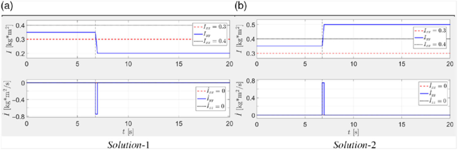
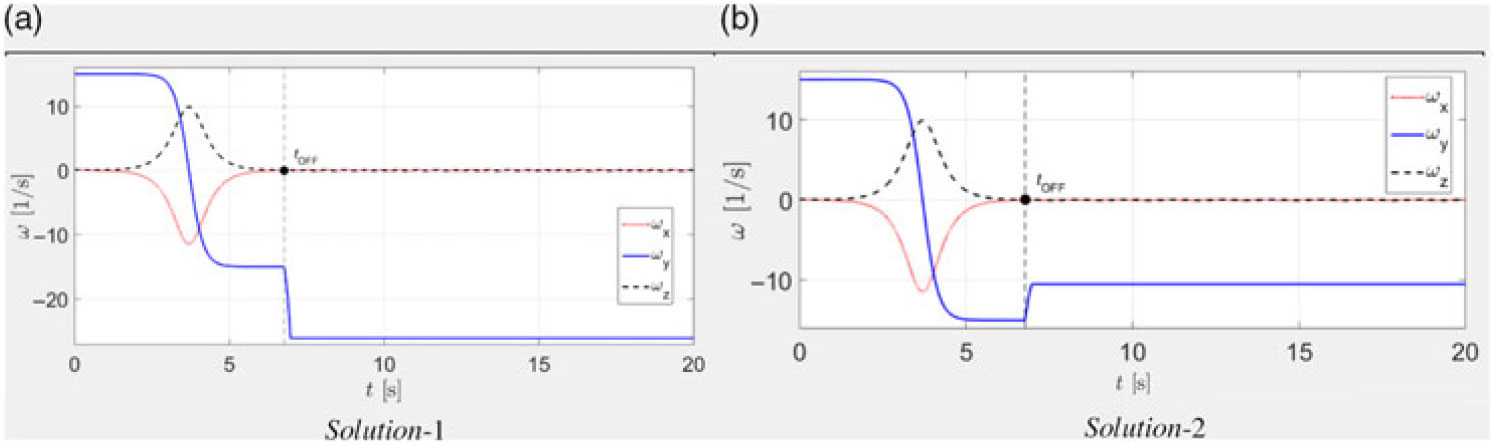
Let us during the flipping motion, at the instant, when the angular velocities ω_x and ω_z are close to zeros, rapidly change the moment of inertia I_yy to its new value of f I_yy = 0.2kg×m².

Then the moment of inertia I_yy stops being the intermediate value, and the rotation about y body axis would becoming stable, without changes in the direction of ω_y.

It has been demonstrated in^{(Reference Trivailo and Kojima2,Reference Trivailo and Kojima5)} that there are two classes of solutions. The new values of the position radii, corresponding to the “solution-1”, can be calculated using Eq. (20):

(26)\begin{equation}{r_x} = 0.1581{\rm{m}};{r_y} = 0.3536{\rm{m}};{r_z} = 0.2739{\rm{m}}.\end{equation}

The spacecraft masses at these radius positions are shown in Fig. 17(a) with dark color.

Figure 17. Graphical representation of solutions for stopping flipping motion. White spheres — initial unstable configuration for y main rotation, black spheres — final stable configuration.

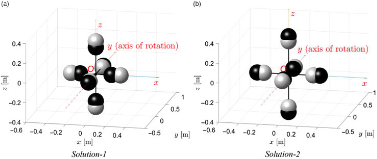
The flipping motion can be also stopped using “solution-2”. For the purpose of the illustration of the concept, let us consider rapid increase of the I_yy from its initial value of 0.35kg×m² to its new value of 0.5kg×m². The new values of the position radii, corresponding to the “solution-2” can be calculated, using Eq. (20):

(27)\begin{equation}{r_x} = 0.3162{\rm{m}};{r_y} = 0.2236{\rm{m}};{r_z} = 0.3873{\rm{m}}.\end{equation}

The spacecraft masses at these radius positions are shown in Fig. 17(b) with dark color.

The morphing of the spacecraft from the initially unstable configuration, associated with the flipping motion, to its final stable configuration and Solution1 and 2 are shown in Fig. 17, where masses for the initial configuration are shown in white, whereas the masses for the final configuration are shown in black color. Summary for both solutions is presented in Table 1. It would be important to note, that in the presented cases, it was not obligatory during the morphing of the system and its transition from the “initial” to “final” states to keep both values of I_xx and I_zz unchanged. However, it was done for purpose, to emphasize the role of the I_yy in the process of stabilisation of the system.

Table 1 Numerical values of the solutions for stopping flipping motion

Results of the corresponding numerical simulations of these two solutions are presented in Fig. 18–20.

Figure 18. Graphical representation of solutions for stopping flipping motion: time histories of the required controlled manipulation with the moment of inertia I_yy.

Figure 19. Graphical representation of solutions for stopping flipping motion: time histories of the ω_x, ω_y, ω_z.

Figure 20. Graphical interpretation of solutions for stopping flipping motion.

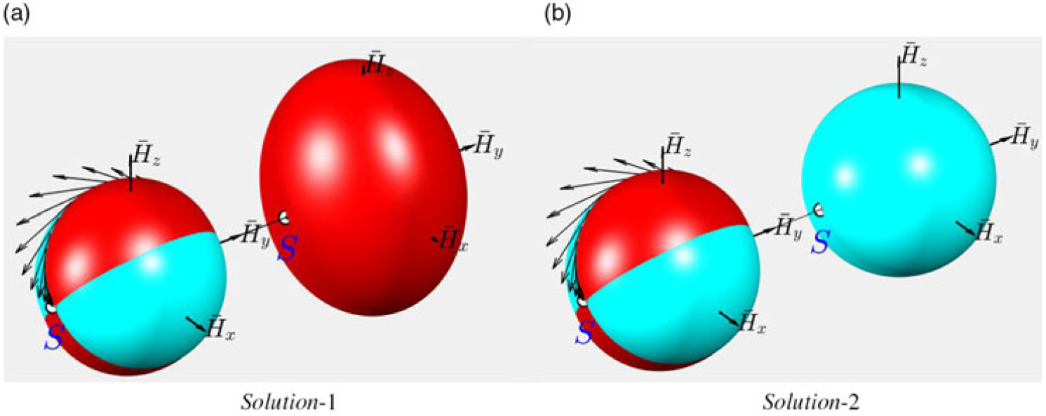
It is interesting to note, that with Solution1, stabilisation of the spinning body is achieved via expansion of the kinetic energy ellipsoid, which completely embraces the angular momentum sphere (see Fig. 20a). On the right part of the Fig. 20a, both surfaces are just only touching each other at the point S and on the opposite side of the y-axis.

However, with Solution-2, stabilisation of the spinning body is achieved via shrinking of the kinetic energy ellipsoid, which becoming completely embraced by the angular momentum sphere (see Fig. 20b). On the right part of the Fig. 20b, both surfaces are just only touching each other at the point S and on the opposite side of the y-axis.

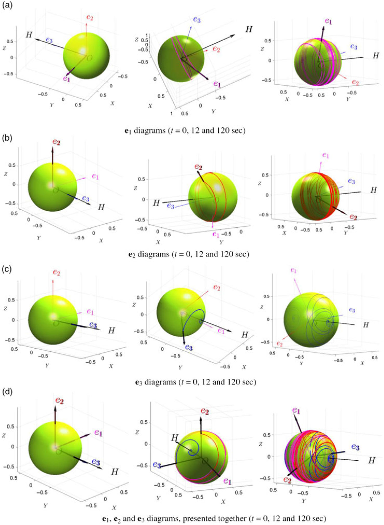
Figure 21. Lines of intersection of the rotating orts e₁e₂ and e₃ with the spherical dome (green), fixed in the global axes system XYZ: ball-of-wool lines.

13.0 INVESTIGATING ORIENTATION OF THE SIDES OF THE SPACECRAFT, EXPOSED TO THE SPECIFIC DIRECTIONS

As spacecraft may have directional sensing equipment, attached to the sides, let us explore possible exposure of this equipment to the specified directions of interest. For this purpose let us introduce a semi-transparent green coloured spherical “dome”, embracing the rotating spacecraft (which, in turn, has its rotating body axes system xyz with unit orts e₁e₂ and e₃). We collocate the centre of the dome (point O) with the centre of the mass of the rotating body. However, most significant, we fix the dome in the global coordinates XYZ, so is not rotating with the body and its body axes xyz. Then we consecutively plot lines of intersection of the rotating orts e₁e₂ and e₃ with the dome. It must be emphasised, that the spheres in Fig. 21 are not the bodies of the spacecraft (which may have any arbitrary shape), but the embracing imaginary domes.

\[\left( {{I_{xx}} = 2,{I_{yy}} = 4,{I_{zz}} = 3,all\,in\,kg\, \times {m^2};{\omega_x} = 0.01,{\omega_y} = 0.01,{\omega_z} = 1,\,all\,in\,rad/s} \right)\]

For the illustration purposes, let us simulate the motion of the spacecraft with the following parameters: I_xx = 2, I_yy = 4, I_zz = 3 (all in kg×m²). Let us for t = 0 align xyz body axes with XYZ global inertial axes as follows: x is aligned with X, y is aligned with Z, z is aligned with −Y. If the spacecraft is installed in orbit with initially provided angular velocities ω _x0 = 0.01, ω _y0 = 0.01, ω _z0 = 1 (all in rad/s), the spacecraft starts flipping along axis z, being an intermediate axis of inertia (as I_xx < I_zz< I_yy).

During this flipping process we trace all intersections of the orts e₁e₂ and e₃ with the dome and present them as continuous lines with different colors. Results are shown in Fig. 21. It should be noted, that for each of the computer screen snap-shots in this figure, the individual viewpoint was selected for better observation of the simulation results. Selection of the viewpoints could be clearly understood using the vector of the angular momentum H as a reference, as it is pointing in the same direction in the global coordinates XYZ for all presented snap-shots.

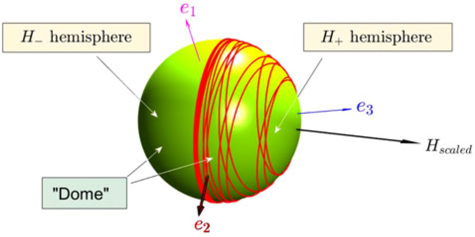
Last image for the e₂ in the middle row in Fig. 22 is remarkably interesting and illustrates our new finding! It shows that y body rotating axis, associated in this example with the maximum moment of inertia, is drawing e₂ intersection lines on the dome only on the hemisphere, bulging towards the angular momentum vector H (we call it H ₊ hemisphere) and is never pointing towards the other hemisphere of the dome (shown as H ₋ hemisphere in Fig. 23). This is valid for the direction of y with positive component of the angular velocity along this direction (ω _y0 > 0). We have run many other various simulations, confirming that it is a general pattern, so the side, perpendicular to the axis with maximum moment of inertia and associated with positive angular velocity component, is never turned away from the vector H direction.

In Fig. 21, initially, vector H is almost aligned with z body axes (which is, in turn, is initially positioned along the –Y global axis), this is because initial values of ω _x0 and ω _z0 (and ultimately H _x0 and H _z0) are small compared with ω _y0 (and ultimately H _y0). Therefore, the 2D plane surface, subdividing H ₊ and H ₋ is almost parallel to the XZ plane. H ₊ and H ₋ are also shown in Fig. 22.

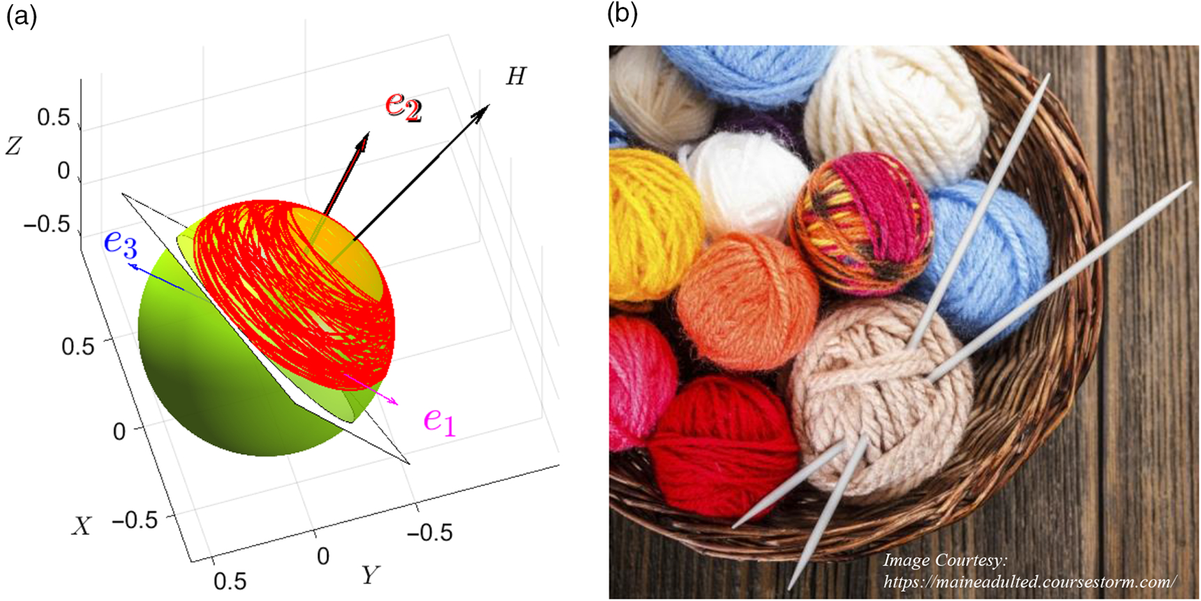
Let us consider additional contrast case with the following parameters: I_xx = 2, I_yy = 4, I_zz = 3 (all in kg×m²) and initial angular velocities ω _x0 = 0.5, ω _y0 = 0.5, ω _z0 = 1 (all in rad/s), which has much more significant initial values of ω _x0 and ω _y0, than in the previous example, hence has large components of H _x0 and H _z0, as compared with H _y0. It results in the subdivision of the dome into two parts (H ₊ and H ₋) by the inclined 2D plane, shown in white in Fig. 23a. Results of the intersection lines of the e₂ ort with the dome are shown in Fig. 23a. They somehow resemble ball of wool (see Fig. 23b), especially with the knitting needles resembling the H and e₂ vectors. However, the simulated resulting ball-of-wool lines are sitting on one hemisphere only! This hemisphere is on the side of the plane, perpendicular to H vector (and we will called it H ₊ hemisphere). The other side of the hemisphere (H ₋) does not have any threads of the ball of wool.

Figure 22. H ₊ and H ₋ hemispheres of the dome (I_xx = 2, I_yy = 4, I_zz = 3, all in kg × m ²; ω_x = 0.01, ω_y = 0.01, ω_z = 1, all in rad/s).

Figure 23. Ball-of-wool lines: (a) Simulation results for the case I_xx = 2, I_yy = 4, I_zz = 3 (all in kg×m²) and initial angular velocities ω _x0 = 0.5, ω _y0 = 0.5, ω _z0 = 1 (all in rad/s), (b) Original balls of wool, which prompted the used analogy and terminology.

This discovered new result can be used in the design of various spacecraft missions. For example, in case of the communication mission, if the spacecraft is installed in orbit with predominant rotation about an intermediate axis of inertia, and is carrying an antenna, it should be ensured that the initial direction of the angular momentum vector H is consistent with the source, sensed by antenna, i.e. with H ₊ hemisphere facing the source, otherwise spacecraft communication would be blanked for all instants of the mission. So, it matters, which side of the spacecraft, perpendicular to the axis with maximum moment of inertia, is selected: one side would be good for utilising antenna, the other side would be inoperable/terminal. The exposure efficiency of the equipment on the selected sides was explored in reference^{(Reference Dorrington and Trivailo22)}.

On the same token, in some other cases, when, for example, the spacecraft is subject to directional adhere conditions (heat, radiation, flying debris) it may be advisable to reinforce the spacecraft, facing the intended H ₋ hemisphere, install the spacecraft in orbit with the direction of the initial angular momentum pointing outwards the danger and place all sensitive equipment on the side, perpendicular to the axis with maximum moment of inertia and with positive component of the angular velocity along this direction (i.e. plus e₂ in the two previously considered illustration cases).

14.0 INERTIAL MORPHING IN ACTION: TWO-PHASE ATTITUDE DYNAMICS MANOEUVER

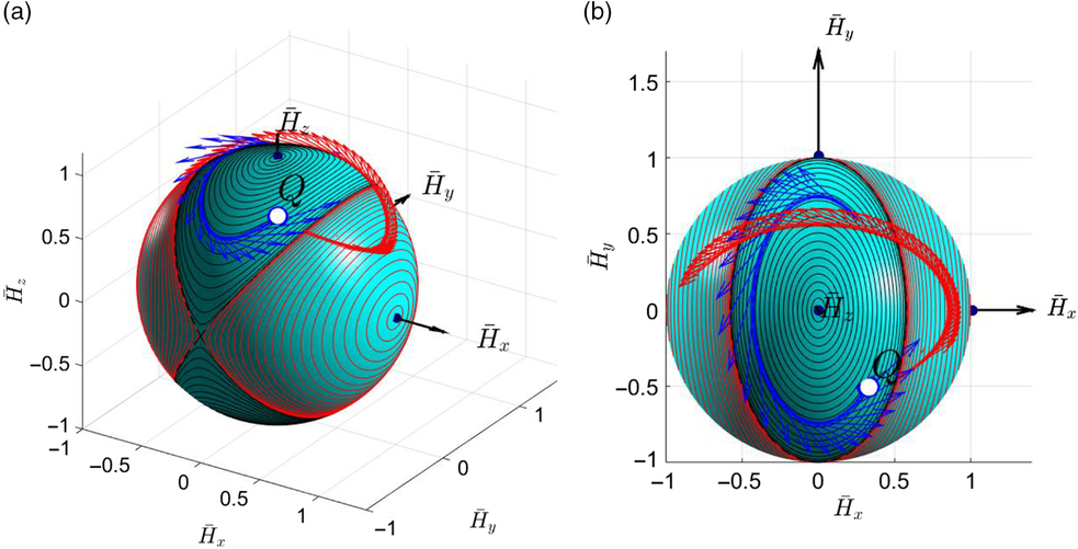
Figure 24(a) shows non-dimensional angular momentum sphere with two separatrices and sets of representative polhodes for the wide range initial conditions. It also shows, as a blue bold line, a specific polhode (or hodograph of the $\overline {\bf{H}} $ vector) for the Phase-1 conditions: I_xx = 2, I_yy = 3, I_zz = 4, ω _x0 = 0.4, ω _y0 = 1, ω _z0 = 0.8.

Figure 24. Non-dimensional angular momentum spheres with polhodes and separatrices and truncated specific hodographs for (a) Phase-1 (before inertial morphing) conditions: I_xx = 2, I_yy = 3, I_zz = 4, ω _x0 = 0.4, ω _y0 = 1, ω _z0 = 0.8; specific hodograph shown with blue line; and (b) Phase-2 (after inertial morphing) conditions: I_xx = 3.5, I_yy = 3, I_zz = 4, $\omega_{xt_{Q}}=0.7133,\ \omega_{yt_{Q}} = -0.7318,\ \omega_{zt_{Q}} = 0.9016,\ t_{Q} =21.5s$; hodograph shown with red line.

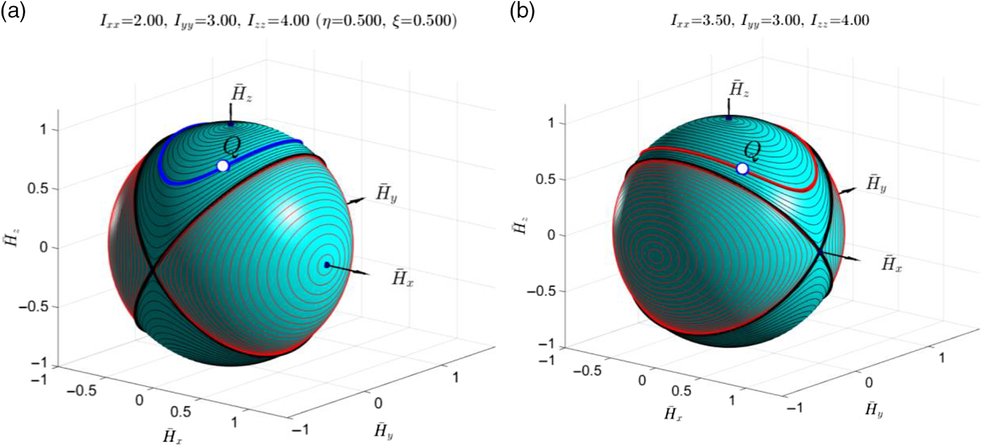
Figure 25. Illustration of the transition between Phase-1 and Phase-2 of the inertial morphing of the system: (a) side 3D view; (b) z-axis 2D view.

If the spacecraft possesses with inertial morphing capabilities, then the switch to any new inertial properties can be simulated and illustrated graphically. Let us assume, for illustration purposes, that the new principal moments of inertia are: I_xx = 3.5, I_yy = 3, I_zz = 4. Then, for the Phase-2, its own non-dimensional angular momentum sphere with two separatrices and sets of representative polhodes (for the wide range initial conditions) can be also produced (see Fig. 25b). Morphing can be applied at any stage during the execution of Phase-1. For certainty, let us also assume that the morphing is rapidly applied at t = 21.5s instant. Then, the new corresponding angular velocities of the spacecraft could be calculated, using equations (21).

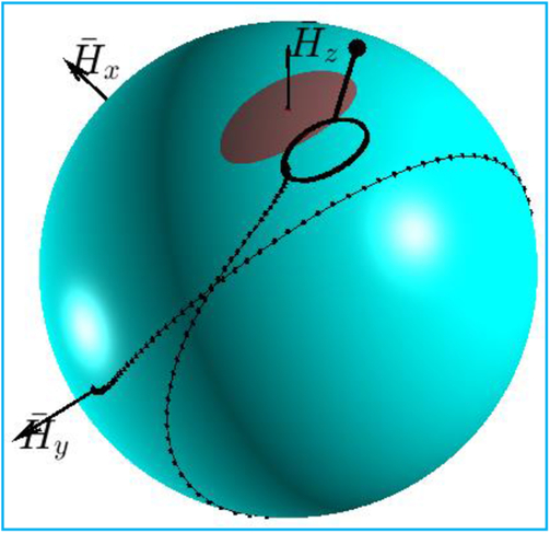
15.0 INERTIAL MORPHING IN ACTION: TRANSFER OF THE TUMBLING MOTION INTO STEADY SPIN ABOUT SELECTED BODY AXIS (THREE-STAGE STABILISATION OF THE SPACECRAFT VIA INERTIAL MORPHING AND UNSTABLE FLIPPING)

Let assume that the spacecraft with given initial values of the moments of inertia (I_xx = 2.5, I_yy = 2.4, I_zz = 3.15) is originally in arbitrary free rotation, involving all three angular velocities, as shown in Fig. 26a.

Figure 26. Illustration of the spacecraft tumbling motion: (a) time history of ω_x, ω_y, ω_z - components of its angular velocity vector ${\boldmath{\vec{\omega}}}$, (b) graphical interpretation of the motion, using KEE and AMS.

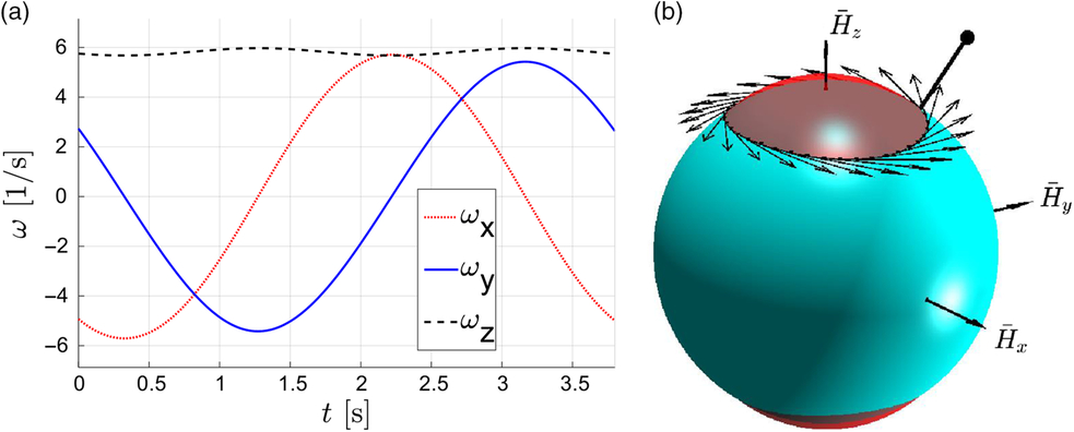
This motion can be visualised, using intersecting kinetic energy ellipsoid and angular momentum sphere, as shown in Fig. 26b. The $\overline {\bf{H}} $ vector of unit genuine length cannot be used for visualization, as its length is equal to one and it would not be seen at any instant, as it would be completely hided by the embracing angular momentum sphere with unit radius. Therefore, for visualisation of the instantaneous orientation of $\overline {\bf{H}} $ in the Fig. 26b, a black line is used with a dot at its end and extruding beyond the surface of the sphere. The hodograph of the vector is shown with a black line on the surface of the angular momentum sphere, coming strictly along the intersection between the AMS and KEE.

Let us set a task to control rotations of the system, via the changes of the values of its principal moments of inertia. In each case of using flipping mode for escaping from the closed smooth polhode, we need to apply change to moments of inertia, which could be calculated based on the parameters of the targeted separatrix, using Eqs. (7)–(8).

An example of complete set of morphings, stabilising the system, being initially in the state of tumbling, is illustrated with Fig. 27.

Figure 27. Three-stage stabilisation of the tumbling spacecraft via morphing: time history of the morphed principal moments of inertia I_xx, I_yy, I_zz.

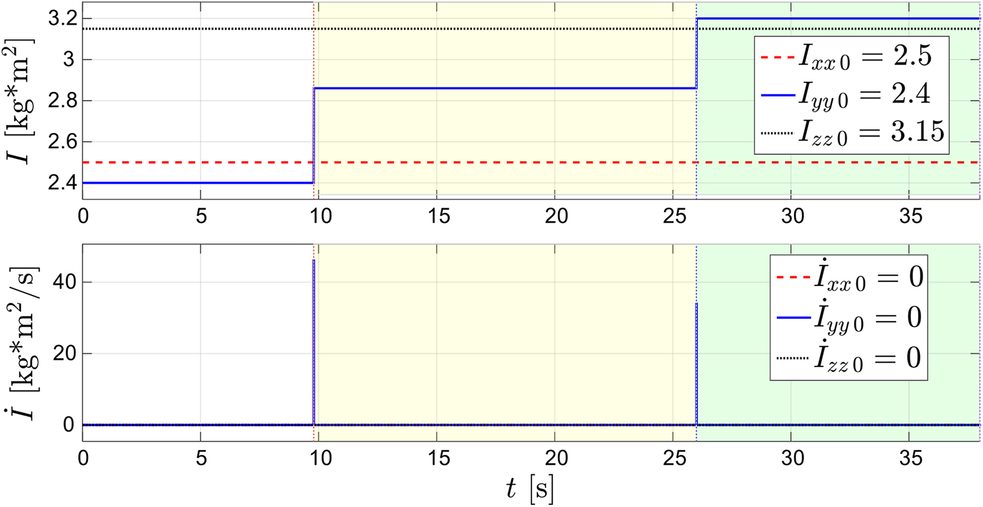
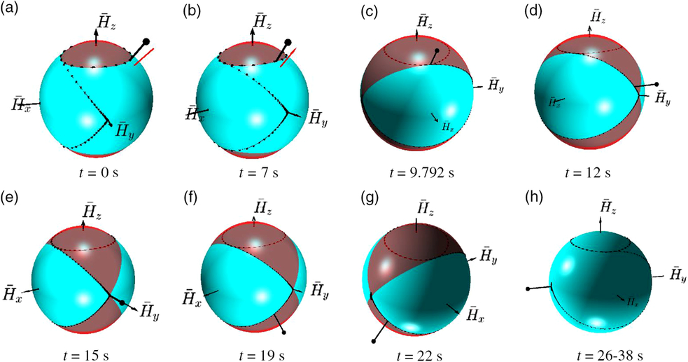
Figure 27 explains the sequence and nature of the inertial changes, deliberately applied to the system. Figure 28 gives consecutive snap-shots from the simulation process, illustrating changes of the kinetic energy ellipsoid and polhodes — resultant feasible trajectories for the angular momentum vector.

Figure 28. Critical instances of spacecraft stabilisation: (a) Start of the simulation; (b) Initially, hodograph is circling around z axis, (c) Stage-1 ends, transition to flipping is initiated, t = 9.792s; (d) approch to the saddle point-1, t = 12s; (e) near the saddle point-1 (possible parking or stabilisation point), t = 15s (f) passing saddle point-1, t = 19s; (g) approach to the saddle point-2, t = 22s; (h) stage-2 ends and third stage starts at t = 26s, parking at the stable saddle point-2 arrtactor is activated, stabilisation is completed.

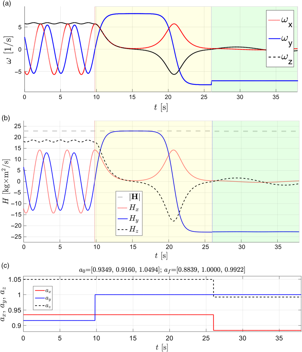
It is interesting to observe, that at the initial stage of the motion of the system, its e₂ body axes ort is drawing a pretty spread trajectory on the “dome” (Fig. 29a). However, after stabilization is completed, this trajectory is essentially reduced to the point (Fig. 29b). Also, at the last stage of the simulation, trajectories for e₁ and e₃ are very close to the equatorial plane, which confirms that the stabilized motion is close to the rotation of the body along the direction of the angular momentum vector. The feature of the example is: the final direction of the y body axes system, selected for stabilisation in this example, is opposite to the direction of H. If the goal of stabilisation was to have them both aligned, then third stage should be activated at instant close to 15s, as evidenced by the Fig. 30b.

Figure 29. Time histories of the (a) ω _x, ω _y, ω _z; (b) H _total, H_x, H_y, H_z and (c) a_x, a_y and a_z during two-stage stabilisation of the tumbling spacecraft via morphing.

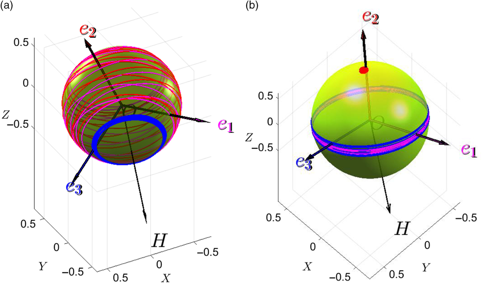
Figure 30. Balls of wool for : (a) the first stage of spacecraft motion with tumbling/coning (t = 0 ÷ 9.792s); (b) last stage of stabilisation of the spacecraft (t = 26 ÷ 38s) with e₁, e₂ and e₃ intersection lines with the dome.

16.0 COMBINED MULTI-PHASE DEMO: CONSECUTIVE PARADE OF ALL THREE ORTHOGONAL INVERSIONS, ASSOCIATED WITH X, Y AND Z BODY AXES

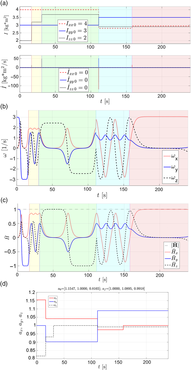
In order to demonstrate capability of the proposed method, in Fig. 31 we present results for a single simulation case, during which the spinning body is reconfigured four times. The carefully selected scenario for the applied inertial morphing (changes in the system, leading to the change of the values of the principal moments of inertia) enables to achieve the flowing:

1. (1) Established flipping motion along y axis (with possibility for y inversion), distinguished with a white background in Fig. 31;

2. (2) Established flipping motion along z axis (with possibility for z inversion), distinguished with green background in Fig. 31;

3. (3) Established flipping motion along x axis (with possibility for x inversion) distinguished with pink background in Fig. 31.

Consequently, it has been demonstrated that the predominant spin can be consecutively passed on to any of the body axis with multiple possibilities for inversion at any stage of the stabilised motion and then stabilisation of the desirable orientation. In other words, if the object had a cube shape, based on this example, it was possible to perform transition of the spinning motion of the cube, allowing exposure of each of its six faces to the direction of the initial angular momentum vector. We call this compound demo case “all-axes inversion parade”.

Figure 31. Time history for the following parameters during four-stage all-axes inversion parade: (a) I_xx, I_yy, I_zz; (b) ω _x, ω _y, ω _z; (c) H _total, H_x, H_y, H_z; (d) a_x, a_y and a_z.

17.0 ENHANCEMENT OF THE REORIENTATION AND CHANGE OF THE SPIN AXIS USING REACTION WHEELS

For completeness of this paper, we need to mention another powerful aspect of further enhancement of the spinning spacecraft attitude control capabilities: adding one or a set of moment reaction wheels, which are often used on various space systems^{(Reference Terui, Kimura, Nagai, Yamamoto, Yoshihara, Yamamoto and Nakasuka23)}.

Differential equations of motion of the spacecraft, equipped with wheels, could be presented as follows:

(28)\begin{align}&\begin{bmatrix}{{I_{xx}}} & \quad 0 & \quad 0 & \quad 0 & \quad 0 & \quad 0 \\ 0 & \quad {{I_{yy}}} & \quad 0 & \quad 0 & \quad 0 & \quad 0 \\ 0 & \quad 0 & \quad {{I_{zz}}} & \quad 0 & \quad 0 & \quad 0 \\ 0 & \quad 0 & \quad 0 & \quad {\sin \theta {\mkern 1mu} {\mkern 1mu} \sin \phi } & \quad {\cos \phi } & \quad 0 \\ 0 & \quad 0 & \quad 0 & \quad {\sin \theta {\mkern 1mu} {\mkern 1mu} \cos \phi } & \quad { - \sin \phi } & \quad 0 \\ 0 & \quad 0 & \quad 0 & \quad {\cos \theta } & \quad 0 & \quad 1\end{bmatrix} \begin{Bmatrix}{{{\dot \omega }_x}} \\ {{{\dot \omega }_y}} \\ {{{\dot \omega }_z}} \\ {\dot \psi } \\ {\dot \theta } \\ {\dot \phi } \end{Bmatrix}\nonumber\\[4pt] &\qquad= \begin{Bmatrix}{({I_{yy}} - {I_{zz}}){\mkern 1mu} {\mkern 1mu} {\omega_y}{\omega_z} - {{\dot I}_{xx}}{\mkern 1mu} {\mkern 1mu} {\omega_x}} \\ {({I_{zz}} - {I_{xx}}){\mkern 1mu} {\mkern 1mu} {\omega_z}{\omega_x} - {{\dot I}_{yy}}{\mkern 1mu} {\mkern 1mu} {\omega_y}} \\ {({I_{xx}} - {I_{yy}}){\mkern 1mu} {\mkern 1mu} {\omega_x}{\omega_y} - {{\dot I}_{zz}}{\mkern 1mu} {\mkern 1mu} {\omega_z}} \\ {{\omega_x}} \\ {{\omega_y}} \\ {{\omega_z}} \end{Bmatrix} - \begin{Bmatrix}{{n_{{\omega_1}}} + {\omega_y}{l_3} - {\omega_z}{l_2}} \\ {{n_{{\omega_2}}} + {\omega_z}{l_1} - {\omega_x}{l_3}} \\ {{n_{{\omega_3}}} + {\omega_x}{l_2} - {\omega_y}{l_1}} \\ 0 \\ 0 \\ 0 \end{Bmatrix}\end{align}

Even simple preliminary cases, involving one wheel and not sophisticated wheel’s controls, enabled us to find significant influence of this enhancement on performance of the system. In particular, it was possible to significantly influence the period of inversion, make inversions asymmetrical (see Fig. 32), etc. The authors intend to explore these capabilities in more detail in the future works.

Figure 32. Shift of stabilisation point, achieved with compoung use of the inertial morphing and reaction wheel.