


1. Introduction
The transport of charged inertial particles in wall-bounded turbulent flows occurs across a wide range of natural and industrial processes. Common examples include electrified dust storms (Zheng et al. Reference Zheng, He and Zhou2004; Zhang & Zhou Reference Zhang and Zhou2020), gas–solid fluidised beds (Pei et al. Reference Pei, Wu and Adams2016), dust ingestion in jet engines (Shinozaki et al. Reference Shinozaki, Roberts, van de Goor and Clyne2013; Diaz-Lopez & Ni Reference Diaz-Lopez and Ni2025) and powder delivery systems (Grosshans & Papalexandris Reference Grosshans and Papalexandris2016). In these processes, solid particles easily accumulate electrical charges through frequent particle–particle or particle–wall collisions (Grosshans & Papalexandris Reference Grosshans and Papalexandris2017; Lacks & Shinbrot Reference Lacks and Shinbrot2019). The resulting electrostatic forces could drastically influence the particle dynamics, including enhancing dust emission in atmospheric boundary layers (Kok & Renno Reference Kok and Renno2008; Esposito et al. Reference Esposito2016), accelerating particle transport in pipe flows (Guha Reference Guha2008; Yao & Capecelatro Reference Yao and Capecelatro2021), initiating particle aggregation and deposition growth (Lee et al. Reference Lee, Waitukaitis, Miskin and Jaeger2015; Sippola et al. Reference Sippola, Kolehmainen, Ozel, Liu, Saarenrinne and Sundaresan2018; Ruan et al. Reference Ruan, Gorman, Li and Ni2022; Gorman et al. Reference Gorman, Ruan and Ni2024) and inducing turbulent modulations (Cui et al. Reference Cui, Zhang and Zheng2024). Moreover, the electric field generated by tribocharged particles may exceed the breakdown limit and trigger electrical discharges, posing potential risks to equipment and personnel safety (Eckhoff Reference Eckhoff2003; Di Renzo & Urzay Reference Di Renzo and Urzay2018). Therefore, investigating the dynamics of charged particles is crucial for revealing the role of electrostatic interactions and advancing our knowledge of the widespread electrostatic phenomena in particle-laden flows.
The transport of neutral inertial particles in wall-bounded flows has been extensively studied and essential physical processes have been revealed (Soldati & Marchioli Reference Soldati and Marchioli2009; Brandt & Coletti Reference Brandt and Coletti2022). The presence of a wall creates a significant gradient of turbulence intensity in the wall-normal direction, driving inertial particles to preferentially migrate towards the wall, which is known as the turbophoresis effect (Caporaloni et al. Reference Caporaloni, Tampieri, Trombetti and Vittori1975; Reeks Reference Reeks1983). Both numerical and experimental studies have shown that the near-wall particle transport is dominated by buffer-layer coherent structures (Ninto & Garcia Reference Ninto and Garcia1996; Marchioli & Soldati Reference Marchioli and Soldati2002). In particular, quasi-streamwise vortices generate sweeps and ejections. Inertial particles brought towards the wall by sweeps are trapped in the viscous layer until they are re-entrained into the outer layer by ejections. As ejection-induced re-entrainment is less efficient, inertial particles tend to accumulate near the wall, leading to the high local concentration. Moreover, the response of inertial particles to the near-wall coherent structures depends on the viscous Stokes number
 $St^+$
, which is defined as the ratio of the particle relaxation time to the viscous time scale, and the strongest near-wall particle accumulation is observed for
$St^+$
, which is defined as the ratio of the particle relaxation time to the viscous time scale, and the strongest near-wall particle accumulation is observed for
 $St^+=10{-}50$
(Sardina et al. Reference Sardina, Schlatter, Brandt, Picano and Casciola2012). After reaching equilibrium, particles oversample fluid motions departing from the wall to balance the turbophoresis drift towards the wall (Picciotto et al. Reference Picciotto, Marchioli and Soldati2005; Picano et al. Reference Picano, Sardina and Casciola2009; Johnson et al. Reference Johnson, Bassenne and Moin2020). In addition, near-wall particles are also found to form elongated streaky structures, corresponding to the low-speed fluid streaks accompanying quasi-streamwise vortices (Rouson & Eaton Reference Rouson and Eaton2001). The dimension of such particle streaks goes up to 500–1000 wall units in the streamwise direction and they are spaced by around 100 wall units in the spanwise direction (Sardina et al. Reference Sardina, Schlatter, Brandt, Picano and Casciola2012; Fong et al. Reference Fong, Amili and Coletti2019). With the increase of the Reynolds number, the scale separation between the small-scale and large-scale structures becomes more significant (Hutchins & Marusic Reference Hutchins and Marusic2007), and large-scale structures located in the outer layer are expected to also contribute to particle transport and accumulation. As a result, while the dynamics of particles with an intermediate
$St^+=10{-}50$
(Sardina et al. Reference Sardina, Schlatter, Brandt, Picano and Casciola2012). After reaching equilibrium, particles oversample fluid motions departing from the wall to balance the turbophoresis drift towards the wall (Picciotto et al. Reference Picciotto, Marchioli and Soldati2005; Picano et al. Reference Picano, Sardina and Casciola2009; Johnson et al. Reference Johnson, Bassenne and Moin2020). In addition, near-wall particles are also found to form elongated streaky structures, corresponding to the low-speed fluid streaks accompanying quasi-streamwise vortices (Rouson & Eaton Reference Rouson and Eaton2001). The dimension of such particle streaks goes up to 500–1000 wall units in the streamwise direction and they are spaced by around 100 wall units in the spanwise direction (Sardina et al. Reference Sardina, Schlatter, Brandt, Picano and Casciola2012; Fong et al. Reference Fong, Amili and Coletti2019). With the increase of the Reynolds number, the scale separation between the small-scale and large-scale structures becomes more significant (Hutchins & Marusic Reference Hutchins and Marusic2007), and large-scale structures located in the outer layer are expected to also contribute to particle transport and accumulation. As a result, while the dynamics of particles with an intermediate
 $St^+$
still correlates with the near-wall vortices, particles with much larger inertia are predominantly driven by large-scale quasi-streamwise vortices whose time scale is comparable to the particle relaxation time, resulting in the formation of multiscale particle streaks in high-Reynolds-number wall-bounded turbulence (Wang & Richter Reference Wang and Richter2019; Berk & Coletti Reference Berk and Coletti2020; Jie et al. Reference Jie, Cui, Xu and Zhao2022; Motoori et al. Reference Motoori, Wong and Goto2022; Berk & Coletti Reference Berk and Coletti2023).
$St^+$
still correlates with the near-wall vortices, particles with much larger inertia are predominantly driven by large-scale quasi-streamwise vortices whose time scale is comparable to the particle relaxation time, resulting in the formation of multiscale particle streaks in high-Reynolds-number wall-bounded turbulence (Wang & Richter Reference Wang and Richter2019; Berk & Coletti Reference Berk and Coletti2020; Jie et al. Reference Jie, Cui, Xu and Zhao2022; Motoori et al. Reference Motoori, Wong and Goto2022; Berk & Coletti Reference Berk and Coletti2023).
Dimensionless deposition velocity
 $k^+$
for neutral particles as a function of the particle Stokes number
$k^+$
for neutral particles as a function of the particle Stokes number
 $St^+$
in previous works. Experimental data are plotted as scatters (
$St^+$
in previous works. Experimental data are plotted as scatters (
 $\square$
: Friedlander & Johnstone Reference Friedlander and Johnstone1957,
$\square$
: Friedlander & Johnstone Reference Friedlander and Johnstone1957,
 $\diamond$
: Sehmel Reference Sehmel1968,
$\diamond$
: Sehmel Reference Sehmel1968,
 $\circ$
: Liu & Agarwal Reference Liu and Agarwal1974,
$\circ$
: Liu & Agarwal Reference Liu and Agarwal1974,
 $+$
: Bernardini Reference Bernardini2014,
$+$
: Bernardini Reference Bernardini2014,
 $\times$
: Fong et al. Reference Fong, Amili and Coletti2019,
$\times$
: Fong et al. Reference Fong, Amili and Coletti2019,
 $\triangle$
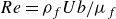
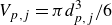
: Forsyth et al. Reference Forsyth, Gillespie and McGilvray2019), while the model prediction by Guha (Reference Guha2008) is shown as the blue solid line.
$\triangle$
: Forsyth et al. Reference Forsyth, Gillespie and McGilvray2019), while the model prediction by Guha (Reference Guha2008) is shown as the blue solid line.
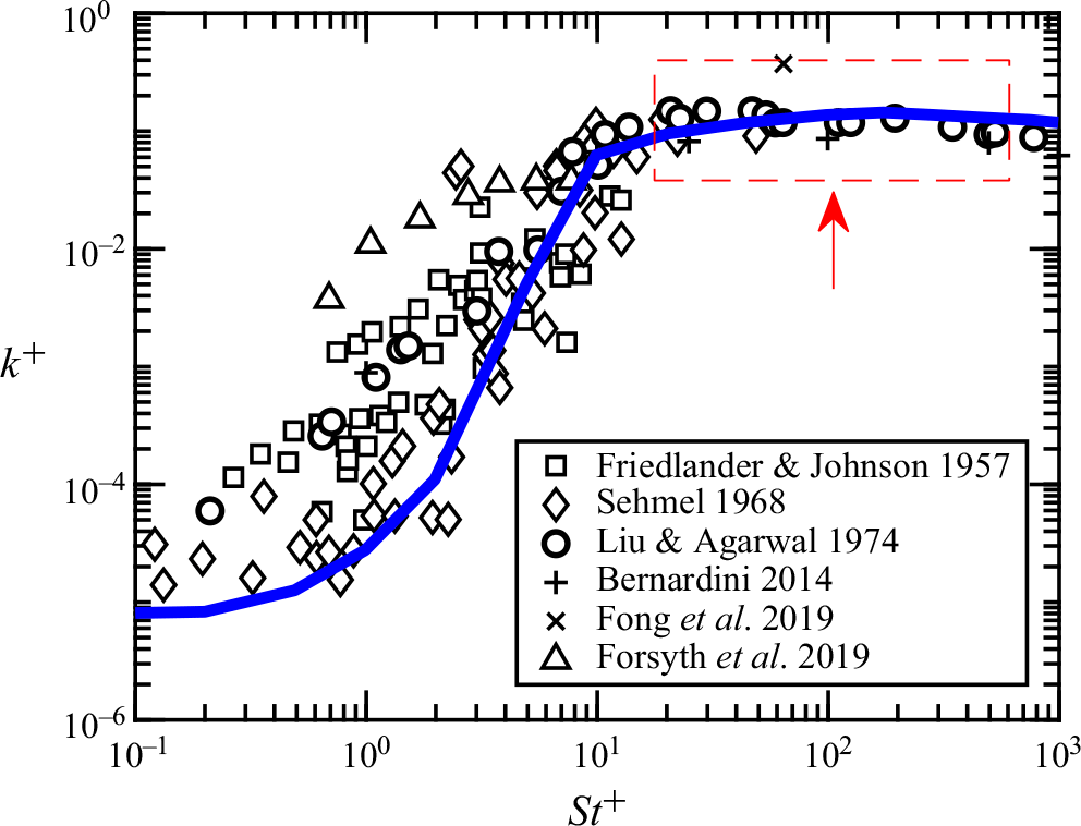
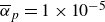
As a result of the complex particle–turbulence interaction, the particle deposition velocity at the walls, which is the primary focus of this study, varies significantly with changes in particle inertia. Figure 1 presents the dimensionless deposition velocity from previous experimental data for neutral particles, along with the prediction based on the model of Guha (Reference Guha2008) represented by the blue solid line. The dimensionless deposition velocity
 $k^+=k/u_{\tau }C_0$
is defined as the flux of particles deposited onto the wall,
$k^+=k/u_{\tau }C_0$
is defined as the flux of particles deposited onto the wall,
 $k$
, normalised by the average particle concentration
$k$
, normalised by the average particle concentration
 $C_0$
and the friction velocity
$C_0$
and the friction velocity
 $u_{\tau }$
. Here,
$u_{\tau }$
. Here,
 $St^+$
is the particle Stokes number defined based on the viscous scales. The experimental data exhibit considerable scatter, spanning several orders of magnitude, which was hypothesised to result from differences in particle charges across experiments. Furthermore, data points within the inertial-particle regime (highlighted by the red window in figure 1) are sparse. However, particles within this regime are highly relevant to problems such as dust ingestion and sandstorms, which will be further investigated in this study.
$St^+$
is the particle Stokes number defined based on the viscous scales. The experimental data exhibit considerable scatter, spanning several orders of magnitude, which was hypothesised to result from differences in particle charges across experiments. Furthermore, data points within the inertial-particle regime (highlighted by the red window in figure 1) are sparse. However, particles within this regime are highly relevant to problems such as dust ingestion and sandstorms, which will be further investigated in this study.
Once particles are charged, the resulting electrostatic interaction makes inertial-particle behaviour more complex. Most existing studies on the dynamics of charged particles in turbulence are conducted in homogeneous isotropic turbulence (HIT). In HIT, the absence of walls means that particle charging only results in the particle–particle (PP) Coulomb force. Under this condition, the significance of the Coulomb force has been quantified using both velocity- and energy-based dimensionless parameters in previous studies. The velocity-based parameter is determined by comparing the electrical migration velocity with the turbulent drift velocity (Lu et al. Reference Lu, Nordsiek and Shaw2010b ; Lu & Shaw Reference Lu and Shaw2015; Di Renzo & Urzay Reference Di Renzo and Urzay2018), while the energy-based parameter compares the electric potential energy with the particle kinetic energy (Lu et al. Reference Lu, Nordsiek, Saw and Shaw2010a ; Boutsikakis et al. Reference Boutsikakis, Fede and Simonin2023; Ruan et al. Reference Ruan, Gorman and Ni2024). When electrostatic effects dominate, both the clustering and relative motion of charged particles are significantly altered (Karnik & Shrimpton Reference Karnik and Shrimpton2012; Yao & Capecelatro Reference Yao and Capecelatro2018; Ruan et al. Reference Ruan, Chen and Li2021; Boutsikakis et al. Reference Boutsikakis, Fede and Simonin2022).
In wall-bounded domains, the electrostatic effects become more complicated because, in addition to the PP electrostatic interaction mentioned above, the particle–wall (PW) electrostatic interaction also plays a role. In Guha (Reference Guha2008), the Eulerian model is extended to account for charged particles under two key assumptions: (i) the particle velocity is modulated solely by the image force and (ii) the particle concentration remains unchanged. Using the image charge model, a charged particle near a conducting wall is subject to the Coulomb force from its own image with the opposing charge at the symmetric location about the wall. The PW interaction is thus attractive, pushing particles towards the wall and increasing the particle deposition velocity. However, the electrostatic force is only found to enhance particle deposition for weak-inertia particles with
 $St^+ \leqslant 10$
, while the deposition of moderate- and large-inertia particles is almost unaffected. The electrostatic-enhanced deposition of small-inertia particles is also confirmed by later direct numerical simulations, where a comprehensive numerical framework is proposed to calculate both PP and PW interactions acting on each particle (Yao & Capecelatro Reference Yao and Capecelatro2021). Meanwhile, when studying the wall-normal accumulation of identically charged particles, Di Renzo et al. (Reference Di Renzo, Johnson, Bassenne, Villafañe and Urzay2019) suggest that it is the collective self-induced electric force (i.e. the PP repulsion) that drives particles towards the wall. And in the later work by Zhang et al. (Reference Zhang, Cui and Zheng2023a
) that studies the behaviour of bidispersed oppositely charged particles, the PP attraction between different particle groups was found to be essential in determining the wall-normal particle distribution compared with the monodispersed case.
$St^+ \leqslant 10$
, while the deposition of moderate- and large-inertia particles is almost unaffected. The electrostatic-enhanced deposition of small-inertia particles is also confirmed by later direct numerical simulations, where a comprehensive numerical framework is proposed to calculate both PP and PW interactions acting on each particle (Yao & Capecelatro Reference Yao and Capecelatro2021). Meanwhile, when studying the wall-normal accumulation of identically charged particles, Di Renzo et al. (Reference Di Renzo, Johnson, Bassenne, Villafañe and Urzay2019) suggest that it is the collective self-induced electric force (i.e. the PP repulsion) that drives particles towards the wall. And in the later work by Zhang et al. (Reference Zhang, Cui and Zheng2023a
) that studies the behaviour of bidispersed oppositely charged particles, the PP attraction between different particle groups was found to be essential in determining the wall-normal particle distribution compared with the monodispersed case.
Despite these recent advances, several questions still remain unresolved. First, while the classic Eulerian framework by Guha (Reference Guha2008) suggests that electrostatic forces only enhance the deposition of small-inertia particles, recent findings by Zhang et al. (Reference Zhang, Cui and Zheng2023a ) indicate that the dynamics of large-inertia particles could also be significantly affected. This raises the question of whether, and how, electrostatic forces promote the transport and deposition of large-inertia particles. In addition, although both PW and PP electrostatic interactions have been found to drive charged particles towards the wall, the relative importance of these two interactions under different conditions has not been thoroughly discussed, and it remains unclear how they each contribute to the overall electrostatic force acting on charged particles. Hence, both assumptions that Guha (Reference Guha2008) has adopted to account for the influence of the electrostatic forces require further examination.
To address the above questions, we perform four-way coupled simulations in this study. The paper is structured as follows. The simulation conditions and the numerical methods are described in § 2. In § 3.1, we first present the effects of electrostatic forces on the wall-normal distribution and the mean velocity of charged particles, followed by a discussion on the wall-normal particle deposition velocity. A statistical approach is introduced in § 3.2 to quantify the contributions of turbophoresis, biased sampling and electrostatic forces to the wall-normal particle distribution. Section 3.3 then provides a detailed explanation of how turbophoresis and biased sampling are modulated. Finally, the competition between PW and PP electrostatic interactions in determining the wall-normal electric field is elucidated in § 3.4.
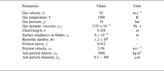
Parameters for dust ingestion problem.
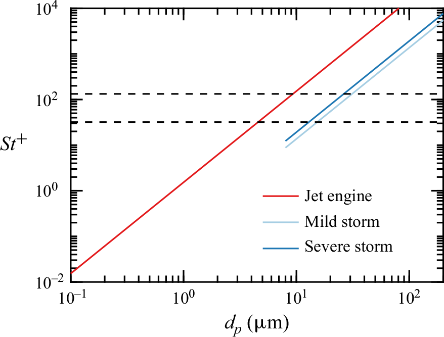
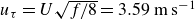
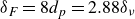
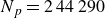
Dependence of particle Stokes number
 $St^+$
on particle size
$St^+$
on particle size
 ${d}_p$
in different applications. Horizontal dashed lines denote
${d}_p$
in different applications. Horizontal dashed lines denote
 $St^+=32$
and
$St^+=32$
and
 $St^+=133$
.
$St^+=133$
.
2. Numerical methods
2.1. Particle parameters
Appropriate parameters for solid particles should be selected to ensure that the particle dynamics falls within the regime relevant to real applications. The aerodynamic response of solid particles to wall-bounded turbulent flows is usually characterised by the viscous Stokes number, defined as the ratio of the particle relaxation time
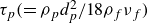 $\tau _p (=\rho _p {d}_p^2/18 \rho _f \nu _f)$
to the viscous time scale
$\tau _p (=\rho _p {d}_p^2/18 \rho _f \nu _f)$
to the viscous time scale
 $\tau _\nu$
 \begin{equation} St^+ = \frac {\tau _p}{\tau _\nu }=\frac {\rho _p}{18 \rho _f} \left ( \frac {{d}_p}{\nu _f /u_\tau } \right )^2 .\end{equation}
Here,
 $\rho _p$
and
$\rho _p$
and
 ${d}_p$
are the particle density and diameter,
${d}_p$
are the particle density and diameter,
 $\rho _f$
and
$\rho _f$
and
 $\nu _f$
are the fluid density and kinematic viscosityand
$\nu _f$
are the fluid density and kinematic viscosityand
 $u_\tau$
denotes the friction velocity.
$u_\tau$
denotes the friction velocity.
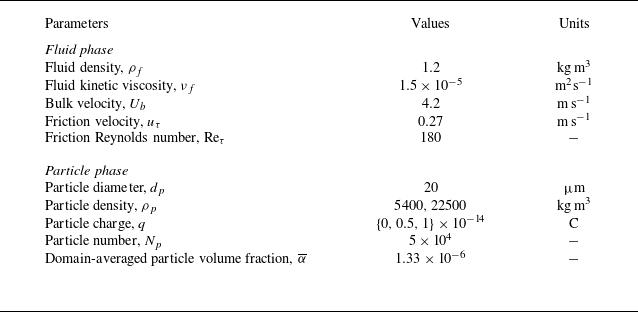
For the deposition of ash particles in jet engines, typical parameters are chosen based on previous works (Taylor Reference Taylor1990; Lawson & Thole Reference Lawson and Thole2011, Reference Lawson and Thole2012; Shinozaki et al. Reference Shinozaki, Roberts, van de Goor and Clyne2013; Sacco et al. Reference Sacco, Bowen, Lundgreen, Bons, Ruggiero, Allen and Bailey2018) and are listed in table 1. The friction factor
 $f=0.012$
is determined by the Reynolds number
$f=0.012$
is determined by the Reynolds number
 $Re=\rho _f U b/ \mu _f$
and the relative roughness
$Re=\rho _f U b/ \mu _f$
and the relative roughness
 $\epsilon _s/D_h$
, where the
$\epsilon _s/D_h$
, where the
 $\epsilon_s$
is the absolute surface roughness, hydraulic diameter
$\epsilon_s$
is the absolute surface roughness, hydraulic diameter
 $D_h$
is assumed to be comparable to the chord length
$D_h$
is assumed to be comparable to the chord length
 $b$
. The friction velocity can thus be estimated as
$b$
. The friction velocity can thus be estimated as
 $u_\tau =U \sqrt {f/8}=3.59 \ {\textrm{m s}^{-1}}$
. Using the ash particle density
$u_\tau =U \sqrt {f/8}=3.59 \ {\textrm{m s}^{-1}}$
. Using the ash particle density
 $\rho _p=1980 \ {\textrm{kg m}^{-3}}$
and the ash particle diameter
$\rho _p=1980 \ {\textrm{kg m}^{-3}}$
and the ash particle diameter
 ${d}_p=0.1{-}100 \ \unicode{x03BC}\textrm{m}$
results in a Stokes number range of
${d}_p=0.1{-}100 \ \unicode{x03BC}\textrm{m}$
results in a Stokes number range of
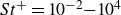 $St^+=10^{-2}{-}10^4$
(red line in figure 2).
$St^+=10^{-2}{-}10^4$
(red line in figure 2).
Additionally, for the transport of dust particles in atmospheric boundary layers, the particle Stokes number can be estimated from field measurement data by Zhang & Zhou (Reference Zhang and Zhou2023). The friction velocity is
 $u_\tau =0.54 \ {\textrm{m s}^{-1}}$
for a mild sandstorm and
$u_\tau =0.54 \ {\textrm{m s}^{-1}}$
for a mild sandstorm and
 $u_\tau =0.64 \ {\textrm{m s}^{-1}}$
for a severe one. Most dust particles lie within the size range
$u_\tau =0.64 \ {\textrm{m s}^{-1}}$
for a severe one. Most dust particles lie within the size range
 $8{-}200 \ \unicode{x03BC}\textrm{m}$
. Assuming a typical dust particle density of
$8{-}200 \ \unicode{x03BC}\textrm{m}$
. Assuming a typical dust particle density of
 $\rho _p=2500 \ {\textrm{kg m}^{-3}}$
,
$\rho _p=2500 \ {\textrm{kg m}^{-3}}$
,
 $St^+$
ranges from
$St^+$
ranges from
 $O(10^1)$
to
$O(10^1)$
to
 $O(10^4)$
(blue lines in figure 2).
$O(10^4)$
(blue lines in figure 2).
Consequently, we choose two typical Stokes numbers,
 $St^+=32$
and
$St^+=32$
and
 $St^+=133$
(dashed lines in figure 2), which are relevant to both applications. Here, moderate-inertia particles with
$St^+=133$
(dashed lines in figure 2), which are relevant to both applications. Here, moderate-inertia particles with
 $St^+=32$
are more responsive to near-wall coherent structures, while large-inertia particles with
$St^+=32$
are more responsive to near-wall coherent structures, while large-inertia particles with
 $St^+=133$
exhibit more ballistic behaviour (Jie et al. Reference Jie, Cui, Xu and Zhao2022).
$St^+=133$
exhibit more ballistic behaviour (Jie et al. Reference Jie, Cui, Xu and Zhao2022).
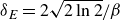
Furthermore, the surface charging density of tribocharged particles is approximately
 $\sigma _c \sim 10^{-5} \ {\textrm{C m}^{-2}}$
(Lee et al. Reference Lee, Waitukaitis, Miskin and Jaeger2015). For typical dust particles with sizes in the tens of microns, the particle charge is around
$\sigma _c \sim 10^{-5} \ {\textrm{C m}^{-2}}$
(Lee et al. Reference Lee, Waitukaitis, Miskin and Jaeger2015). For typical dust particles with sizes in the tens of microns, the particle charge is around
 $10^{-15}{-}10^{-14} \ \textrm{C}$
. As a result, the particle charge
$10^{-15}{-}10^{-14} \ \textrm{C}$
. As a result, the particle charge
 $q$
in the simulations is set around this level, which is comparable to values used in previous studies (Zhang et al. Reference Zhang, Cui and Zheng2023a
; Ruan et al. Reference Ruan, Gorman and Ni2024). In addition, since our focus is on the effects of electrostatic force, other significant forces, such as gravity and lift force (Marchioli et al. Reference Marchioli, Picciotto and Soldati2007; Berk & Coletti Reference Berk and Coletti2020; Gao et al. Reference Gao, Shi, Parsani and Costa2024), are not included in this study.
$q$
in the simulations is set around this level, which is comparable to values used in previous studies (Zhang et al. Reference Zhang, Cui and Zheng2023a
; Ruan et al. Reference Ruan, Gorman and Ni2024). In addition, since our focus is on the effects of electrostatic force, other significant forces, such as gravity and lift force (Marchioli et al. Reference Marchioli, Picciotto and Soldati2007; Berk & Coletti Reference Berk and Coletti2020; Gao et al. Reference Gao, Shi, Parsani and Costa2024), are not included in this study.
2.2. Simulation system
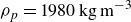
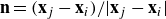
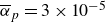
Snapshot of the simulation system. The colour bar represents the magnitude of the fluid velocity
 $|\mathbf{u}_f|$
. Particles are plotted as grey spheres with exaggerated sizes. For clarity, only a small portion of particles near the bottom wall is shown.
$|\mathbf{u}_f|$
. Particles are plotted as grey spheres with exaggerated sizes. For clarity, only a small portion of particles near the bottom wall is shown.
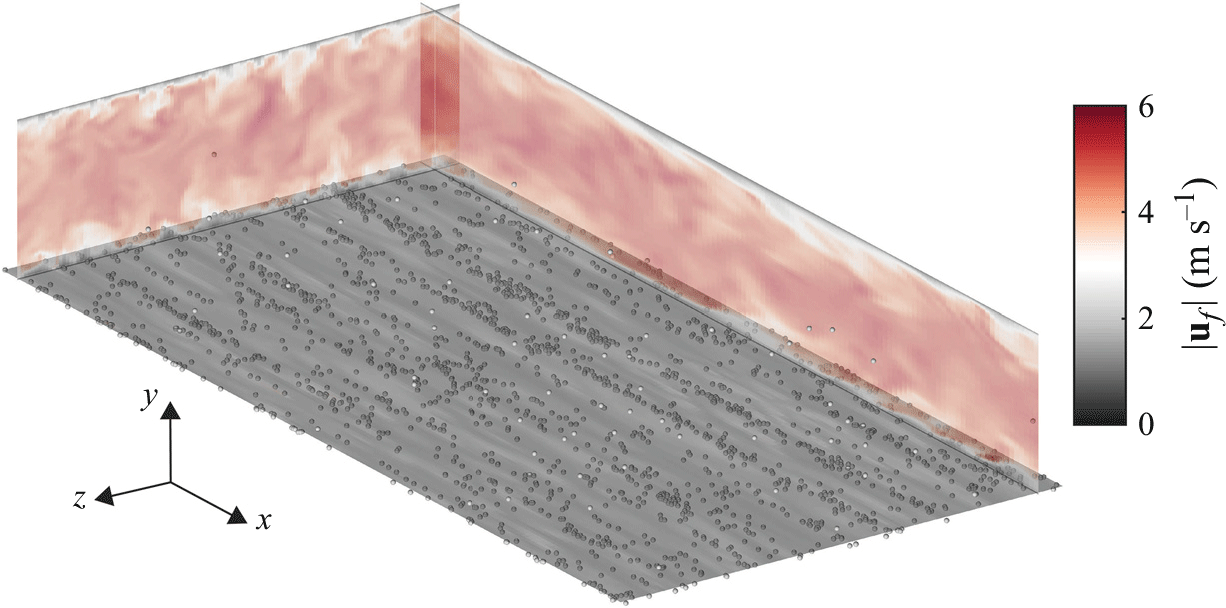
As shown in figure 3, the simulation system is a particle-laden turbulent channel flow between two infinite parallel walls, and the simulation parameters are listed in table 2. The dimension of the computation domain is
 $L_x \times L_y \times L_z = 4\pi \delta \times 2 \delta \times 2\pi \delta$
with
$L_x \times L_y \times L_z = 4\pi \delta \times 2 \delta \times 2\pi \delta$
with
 $\delta =0.01 \ \textrm{m}$
being the half-channel height. The periodic boundary condition is applied to both the streamwise (
$\delta =0.01 \ \textrm{m}$
being the half-channel height. The periodic boundary condition is applied to both the streamwise (
 $x$
) and spanwise (
$x$
) and spanwise (
 $z$
) directions, while the no-slip boundary condition is applied to the wall-normal direction (
$z$
) directions, while the no-slip boundary condition is applied to the wall-normal direction (
 $y$
). The constant bulk velocity of the fluid phase is
$y$
). The constant bulk velocity of the fluid phase is
 $U_b=4.2 \ {\textrm{m s}^{-1}}$
, and the friction Reynolds number is
$U_b=4.2 \ {\textrm{m s}^{-1}}$
, and the friction Reynolds number is
 $Re_{\tau }=u_{\tau } \delta /\nu _f =180$
, with
$Re_{\tau }=u_{\tau } \delta /\nu _f =180$
, with
 $u_{\tau }$
and
$u_{\tau }$
and
 $\nu _f$
being the friction velocity and the fluid kinematic viscosity, respectively. The grid number is
$\nu _f$
being the friction velocity and the fluid kinematic viscosity, respectively. The grid number is
 $N_x \times N_y \times N_z = 128^3$
. The grid is uniform in both x and z directions, and the non-uniform wall-normal grid is defined by the hyperbolic tangent function with the stretching factor
$N_x \times N_y \times N_z = 128^3$
. The grid is uniform in both x and z directions, and the non-uniform wall-normal grid is defined by the hyperbolic tangent function with the stretching factor
 $S=1.9$
(Marchioli et al. Reference Marchioli, Soldati, Kuerten, Arcen, Taniere, Goldensoph, Squires, Cargnelutti and Portela2008). This leads to a grid spacing of
$S=1.9$
(Marchioli et al. Reference Marchioli, Soldati, Kuerten, Arcen, Taniere, Goldensoph, Squires, Cargnelutti and Portela2008). This leads to a grid spacing of
 $\Delta x^+ = 17.67$
,
$\Delta x^+ = 17.67$
,
 $\Delta z^+ = 8.84$
and
$\Delta z^+ = 8.84$
and
 $\Delta y^+ = 0.49{-}5.58$
. The grid resolution has been assessed in Appendix A, and is shown to be sufficient for the fluid flow investigated in this study. Hereinafter, variables normalised by the wall units (i.e. the friction velocity
$\Delta y^+ = 0.49{-}5.58$
. The grid resolution has been assessed in Appendix A, and is shown to be sufficient for the fluid flow investigated in this study. Hereinafter, variables normalised by the wall units (i.e. the friction velocity
 $u_{\tau }$
, the viscous length scales
$u_{\tau }$
, the viscous length scales
 $\delta _{\nu }=\nu _f / u_{\tau }$
and the viscous time scale
$\delta _{\nu }=\nu _f / u_{\tau }$
and the viscous time scale
 $\tau _{\nu }=\nu _f / u_{\tau }^2$
) are presented with the superscript
$\tau _{\nu }=\nu _f / u_{\tau }^2$
) are presented with the superscript
 $+$
.
$+$
.
Simulation parameters.
The total number of particles in the domain is
 $N_p=5 \times 10^4$
, and the particles are assumed to be heavy and small. The particle diameter is fixed at
$N_p=5 \times 10^4$
, and the particles are assumed to be heavy and small. The particle diameter is fixed at
 ${d}_p=20 \ \unicode{x03BC}\textrm{m}$
(
${d}_p=20 \ \unicode{x03BC}\textrm{m}$
(
 ${d}_p^+=0.36$
), so the domain-averaged particle volume fraction is a constant (
${d}_p^+=0.36$
), so the domain-averaged particle volume fraction is a constant (
 $\overline {\alpha }=1.33 \times 10^{-6}$
) and falls within the dilute regime. The particle Stokes number is controlled by adjusting the particle density.
$\overline {\alpha }=1.33 \times 10^{-6}$
) and falls within the dilute regime. The particle Stokes number is controlled by adjusting the particle density.
2.3. Fluid phase
In this study, the volume-filtered Eulerian–Lagrangian framework is employed to simulate particle-laden turbulent channel flow. The incompressible fluid motion is solved using the open-source solver NGA2 (Desjardins et al. Reference Desjardins, Blanquart, Balarac and Pitsch2008; Capecelatro & Desjardins Reference Capecelatro and Desjardins2013). A brief derivation of the volume-filtered governing equation for the fluid phase, starting from the standard point-wise equations, is provided in Appendix B1. The associated model closure problem is further discussed in Appendix B2. Finally, the volume-filtered governing equations of the fluid phase used in this study are given by
 \begin{equation} \frac {\partial {\alpha }}{\partial t} + \boldsymbol{\nabla} \cdot (\alpha \mathbf{u}_f) = 0, \end{equation}
 \begin{equation} \frac {\partial (\alpha \mathbf{u}_f)}{\partial t} + \boldsymbol{\nabla} \cdot (\alpha \mathbf{u}_f \otimes \mathbf{u}_f) = \boldsymbol{\nabla} \cdot \boldsymbol{\tau } + \mathbf{f}_{F} + \mathbf{f}_{P}. \end{equation}
Here,
 $\alpha$
and
$\alpha$
and
 $\mathbf{u}_f$
are the fluid volume fraction and the flow velocity. The fluid stress is
$\mathbf{u}_f$
are the fluid volume fraction and the flow velocity. The fluid stress is
 ${\tau }=-p/\rho _f \mathbf{I} + \nu _f [(\boldsymbol{\nabla} \textrm{u}_f+{\boldsymbol{\nabla} \textrm{u}_f}^T) - 2(\boldsymbol{\nabla} \cdot \mathbf{u}_f)\mathbf{I}/3]$
with
${\tau }=-p/\rho _f \mathbf{I} + \nu _f [(\boldsymbol{\nabla} \textrm{u}_f+{\boldsymbol{\nabla} \textrm{u}_f}^T) - 2(\boldsymbol{\nabla} \cdot \mathbf{u}_f)\mathbf{I}/3]$
with
 $p$
,
$p$
,
 $\rho _f$
,
$\rho _f$
,
 $\nu _f$
being the pressure, density and kinematic viscosity of the fluid phase, respectively,
$\nu _f$
being the pressure, density and kinematic viscosity of the fluid phase, respectively,
 $\mathbf{I}$
is the identity tensor,
$\mathbf{I}$
is the identity tensor,
 $\mathbf{f}_{F}$
is the streamwise forcing term that maintains a constant mass flow rate and
$\mathbf{f}_{F}$
is the streamwise forcing term that maintains a constant mass flow rate and
 $\mathbf{f}_{P}$
is the momentum exchange term due to inter-phase coupling.
$\mathbf{f}_{P}$
is the momentum exchange term due to inter-phase coupling.
The volume-filtered Navier–Stokes equations are solved on a staggered grid with second-order spatial accuracy for both the convective and the viscous term, and are advanced using the second-order semi-implicit Crank–Nicolson scheme (Pierce Reference Pierce2001). The pressure Poisson equation is solved by a multigrid solver using the preconditioned conjugate gradient method (Falgout & Yang Reference Falgout and Yang2002).
2.4. Particle phase
The suspended particles are treated as spheres and their movements are simulated using the Lagrangian approach. Both particle translation and rotation are updated considering the exerted forces/torques as
 \begin{equation} m_i \frac {\textrm{d}\mathbf{v}_i}{\textrm{d}t} = \mathbf{F}_i^{F} + \mathbf{F}_i^{C} + \mathbf{F}_i^{E}, \end{equation}
 \begin{equation} I_i \frac {\textrm{d}\boldsymbol{\Omega }_i}{\textrm{d}t} = \mathbf{T}_i^{F} + \mathbf{T}_i^{C}. \end{equation}
Here,
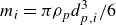 $m_i= \pi \rho _p {d}_{{p},i}^3/6$
and
$m_i= \pi \rho _p {d}_{{p},i}^3/6$
and
 $I=m_i {d}_{{p},i}^2/10$
are the mass and the momentum of inertia of particle
$I=m_i {d}_{{p},i}^2/10$
are the mass and the momentum of inertia of particle
 $i$
,
$i$
,
 $\mathbf{v}_i$
is the particle velocity,
$\mathbf{v}_i$
is the particle velocity,
 $\boldsymbol{\Omega }_i$
is the rotation rate and
$\boldsymbol{\Omega }_i$
is the rotation rate and
 $\mathbf{F}_i$
and
$\mathbf{F}_i$
and
 $\mathbf{T}_i$
denote the acted force and torque. The superscripts
$\mathbf{T}_i$
denote the acted force and torque. The superscripts
 $F$
,
$F$
,
 $C$
and
$C$
and
 $E$
refer to fluid force/torque, collision force/torque and electrostatic force, respectively.
$E$
refer to fluid force/torque, collision force/torque and electrostatic force, respectively.
In this study, gravity is intentionally neglected. The presence of wall-normal gravity would introduce an additional vertical migration velocity, increasing particle flux towards the bottom wall and decreasing it towards the top wall (Marchioli et al. Reference Marchioli, Picciotto and Soldati2007; Berk & Coletti Reference Berk and Coletti2020). In contrast, as will be shown below, both the turbophoresis effect and the electrostatic force tend to enhance particle deposition towards both walls. Consequently, incorporating gravity could break the symmetry of the system, with the steady-state statistics being governed by a complex interplay between gravity, electrostatics and particle-turbulence interactions. This added complexity could make it more challenging to isolate and clarify the specific role of electrostatic forces. For this reason, we have intentionally neglected gravity, ensuring that any changes in the particle dynamics between neutral and charged cases can be solely attributed to the influence of electrostatic forces.
2.4.1. Particle–fluid interaction
The particles considered in this study are significantly heavier than the fluid (
 $\rho _p/\rho _f \sim O(10^3)$
), and their size is small compared with the viscous length (
$\rho _p/\rho _f \sim O(10^3)$
), and their size is small compared with the viscous length (
 ${d}_p/\delta _\nu$
= 0.36). Given that the length scales of near-wall turbulent structures are at least tens of
${d}_p/\delta _\nu$
= 0.36). Given that the length scales of near-wall turbulent structures are at least tens of
 $\delta _\nu$
, the solid particles can be treated as point particles.
$\delta _\nu$
, the solid particles can be treated as point particles.
For an individual particle
 $i$
, the full fluid force can be obtained by integrating the fluid stress over the particle surface. As the volume-filtered framework is used, the fluid force can be decomposed into the contribution from the resolved and unsolved stress as
$i$
, the full fluid force can be obtained by integrating the fluid stress over the particle surface. As the volume-filtered framework is used, the fluid force can be decomposed into the contribution from the resolved and unsolved stress as
 \begin{align} \mathbf{F}_i^F=\int _{\mathcal{S}_i}\boldsymbol{\tau }\cdot \mathbf{n} \textrm{d}\mathbf{y}=\int _{\mathcal{S}_i} (\overline {\boldsymbol{\tau }} + \boldsymbol{\tau }^\prime ) \cdot \mathbf{n} \textrm{d}\mathbf{y} = \int _{\mathcal{V}_i} \boldsymbol{\nabla} \cdot \overline {\boldsymbol{\tau }} \textrm{d}\mathbf{y} + \int _{\mathcal{S}_i} \boldsymbol{\tau }^\prime \cdot \mathbf{n} \textrm{d}\mathbf{y}. \end{align}
If the particle size is much smaller than the filter size, as in this study,
 $\boldsymbol{\nabla} \cdot \overline {\boldsymbol{\tau }}$
varies little at the particle scale and can be taken out of the integral. The fluid force then becomes
$\boldsymbol{\nabla} \cdot \overline {\boldsymbol{\tau }}$
varies little at the particle scale and can be taken out of the integral. The fluid force then becomes
 \begin{align} \mathbf{F}_i^F=\int _{\mathcal{V}_i} \boldsymbol{\nabla} \cdot \overline {\boldsymbol{\tau }} \textrm{d}\mathbf{y} + \int _{\mathcal{S}_i} \boldsymbol{\tau }^\prime \cdot \mathbf{n} \textrm{d}\mathbf{y} \approx \boldsymbol{\nabla} \cdot \overline {\boldsymbol{\tau }} \mathcal{V}_i +\int _{\mathcal{S}_i} \boldsymbol{\tau }^\prime \cdot \mathbf{n} \textrm{d}\mathbf{y}. \end{align}
Here,
 $\mathcal{V}_i$
is the volume of particle
$\mathcal{V}_i$
is the volume of particle
 $i$
. The fluid force due to the residual stress,
$i$
. The fluid force due to the residual stress,
 $\int _{\mathcal{S}_i} \boldsymbol{\tau }^\prime \cdot \mathbf{n} \textrm{d}\mathbf{y}$
, needs to be modelled. As discussed in Appendix B, the eddy viscosity at the unresolved scale,
$\int _{\mathcal{S}_i} \boldsymbol{\tau }^\prime \cdot \mathbf{n} \textrm{d}\mathbf{y}$
, needs to be modelled. As discussed in Appendix B, the eddy viscosity at the unresolved scale,
 $\nu _t$
, is much smaller than the fluid molecular viscosity,
$\nu _t$
, is much smaller than the fluid molecular viscosity,
 $\nu _f$
, indicating that the unresolved flow around the particle is essentially laminar. Based on these considerations, the fluid force is modelled using the Maxey–Riley equation (Maxey & Riley Reference Maxey and Riley1983). Since the fluid drag is the dominant fluid force, other fluid forces are neglected. A detailed comparison of the fluid drag with other forces, such as lift force and short-range lubrication force, is provided in Appendix C. The resolved fluid force,
$\nu _f$
, indicating that the unresolved flow around the particle is essentially laminar. Based on these considerations, the fluid force is modelled using the Maxey–Riley equation (Maxey & Riley Reference Maxey and Riley1983). Since the fluid drag is the dominant fluid force, other fluid forces are neglected. A detailed comparison of the fluid drag with other forces, such as lift force and short-range lubrication force, is provided in Appendix C. The resolved fluid force,
 $\boldsymbol{\nabla} \cdot \overline {\boldsymbol{\tau }} \mathcal{V}_i$
, is also negligible compared with fluid drag for two reasons. First, the filter size
$\boldsymbol{\nabla} \cdot \overline {\boldsymbol{\tau }} \mathcal{V}_i$
, is also negligible compared with fluid drag for two reasons. First, the filter size
 $\delta _F$
is much larger than the particle size
$\delta _F$
is much larger than the particle size
 ${d}_p$
, resulting in a small divergence of the filtered stress. Second, the particle size
${d}_p$
, resulting in a small divergence of the filtered stress. Second, the particle size
 ${d}_p$
is small, leading to an even smaller volume
${d}_p$
is small, leading to an even smaller volume
 $\mathcal{V}$
. Preliminary tests show that the ratio of the resolved fluid force to the drag force,
$\mathcal{V}$
. Preliminary tests show that the ratio of the resolved fluid force to the drag force,
 $|\boldsymbol{\nabla} \cdot \overline {\boldsymbol{\tau }} \mathcal{V}|/F_{d}$
, is only 0.036 for
$|\boldsymbol{\nabla} \cdot \overline {\boldsymbol{\tau }} \mathcal{V}|/F_{d}$
, is only 0.036 for
 $St^+=32$
and 0.001 for
$St^+=32$
and 0.001 for
 $St^+=133$
. Consequently, we only consider fluid drag in this study, and the fluid force and torque are given as
$St^+=133$
. Consequently, we only consider fluid drag in this study, and the fluid force and torque are given as
 \begin{equation} \mathbf{F}_i^F = -3 \pi \mu _f {d}_{p,i} \left (\mathbf{v}_i-\mathbf{u}_f(\mathbf{x}_i)\right ) f_I, \end{equation}
 \begin{equation} \mathbf{T}_i^F = -\pi \mu _f {d}_{p,i}^3 \left (\boldsymbol{\Omega }_i-\frac {1}{2} \boldsymbol{\omega }(\mathbf{x}_i)\right ). \end{equation}
Here,
 $\mu _f$
is the fluid dynamic viscosity,
$\mu _f$
is the fluid dynamic viscosity,
 $\mathbf{u}_f(\mathbf{x}_i)$
and
$\mathbf{u}_f(\mathbf{x}_i)$
and
 $\boldsymbol{\omega }(\mathbf{x}_i)$
are the fluid velocity and vorticity interpolated at the particle location using trilinear interpolation. The influence of the order of the interpolation scheme has been discussed in Appendix D. In two-way coupled simulations, the accurate calculation of fluid drag requires the undisturbed fluid velocity
$\boldsymbol{\omega }(\mathbf{x}_i)$
are the fluid velocity and vorticity interpolated at the particle location using trilinear interpolation. The influence of the order of the interpolation scheme has been discussed in Appendix D. In two-way coupled simulations, the accurate calculation of fluid drag requires the undisturbed fluid velocity
 $\tilde {\mathbf{u}}_f(\mathbf{x}_p)$
at the particle location, because the feedback force from the target particle itself perturbs surrounding fluid flow. As a result, the local fluid velocity,
$\tilde {\mathbf{u}}_f(\mathbf{x}_p)$
at the particle location, because the feedback force from the target particle itself perturbs surrounding fluid flow. As a result, the local fluid velocity,
 $\mathbf{u}_f(\mathbf{x}_p) (\neq \tilde {\mathbf{u}}_f(\mathbf{x}_p))$
, is effectively disturbed (or ‘contaminated’), leading to an underestimated slip velocity and, consequently, a reduced drag force. To address this issue, various correction schemes have been proposed for both point-particle (Gualtieri et al. Reference Gualtieri, Picano, Sardina and Casciola2015; Horwitz & Mani Reference Horwitz and Mani2020) and finite-size particle simulations (Balachandar & Liu Reference Balachandar and Liu2023) to recover the undisturbed fluid velocity
$\mathbf{u}_f(\mathbf{x}_p) (\neq \tilde {\mathbf{u}}_f(\mathbf{x}_p))$
, is effectively disturbed (or ‘contaminated’), leading to an underestimated slip velocity and, consequently, a reduced drag force. To address this issue, various correction schemes have been proposed for both point-particle (Gualtieri et al. Reference Gualtieri, Picano, Sardina and Casciola2015; Horwitz & Mani Reference Horwitz and Mani2020) and finite-size particle simulations (Balachandar & Liu Reference Balachandar and Liu2023) to recover the undisturbed fluid velocity
 $\tilde {u}_f(x_p)$
and ensure physically accurate results. In this work, however, because of the large size ratio between the Gaussian filter length and the particle size
$\tilde {u}_f(x_p)$
and ensure physically accurate results. In this work, however, because of the large size ratio between the Gaussian filter length and the particle size
 $\delta _F/{d}_p=8$
, the error in drag force caused by self-induced disturbance is less significant, so the correction scheme is not applied. Detailed discussions on the correction scheme of the undisturbed fluid velocity and its influences are given in Appendix E. To account for the effect of fluid inertia, the drag force is corrected using the Schiller–Naumann correction factor,
$\delta _F/{d}_p=8$
, the error in drag force caused by self-induced disturbance is less significant, so the correction scheme is not applied. Detailed discussions on the correction scheme of the undisturbed fluid velocity and its influences are given in Appendix E. To account for the effect of fluid inertia, the drag force is corrected using the Schiller–Naumann correction factor,
 $f_I$
, which writes
$f_I$
, which writes
 \begin{equation} f_I=1+0.15 Re_p^{0.687}. \end{equation}
Here, the particle Reynolds number is defined as
 $Re_p=|\mathbf{v}_i-\mathbf{u}_f(\mathbf{x}_i)| d_{p,i}/\nu _f$
.
$Re_p=|\mathbf{v}_i-\mathbf{u}_f(\mathbf{x}_i)| d_{p,i}/\nu _f$
.
To consider the flow modulation caused by the particle phase, both the fluid volume fraction
 $\alpha$
and the momentum transfer term
$\alpha$
and the momentum transfer term
 $\mathbf{f}_P$
in (2.2) are computed as follows:
$\mathbf{f}_P$
in (2.2) are computed as follows:
 \begin{equation} \alpha (\mathbf{X}_i) = 1- \frac {1}{V_{cell,i}} \sum _{j=1}^{N_p} G_F(|\mathbf{X}_i-\mathbf{x}_j|) V_{p,j}, \end{equation}
 \begin{equation} \mathbf{f}_P (\mathbf{X}_i) = -\frac {1}{\rho _f V_{cell,i}} \sum _{j=1}^{N_p} G_F(|\mathbf{X}_i-\mathbf{x}_j|) \mathbf{F}^F_{j}. \end{equation}
Here,
 $\mathbf{X}_i$
is the location of the
$\mathbf{X}_i$
is the location of the
 $i$
th grid cell,
$i$
th grid cell,
 $V_{p,j}=\pi {d}_{p,j}^3 /6$
is the volume of the
$V_{p,j}=\pi {d}_{p,j}^3 /6$
is the volume of the
 $j$
th particle and
$j$
th particle and
 $G_F$
is the fluid Gaussian filter that distributes the Lagrangian quantities (i.e.
$G_F$
is the fluid Gaussian filter that distributes the Lagrangian quantities (i.e.
 $V_{p,j}$
and
$V_{p,j}$
and
 $\mathbf{F}^F_{j}$
) to the Cartesian mesh. The characteristic fluid filtering length
$\mathbf{F}^F_{j}$
) to the Cartesian mesh. The characteristic fluid filtering length
 $\delta _F$
, defined as the full width of the fluid Gaussian filter
$\delta _F$
, defined as the full width of the fluid Gaussian filter
 $G_F$
at the half-height, is chosen as
$G_F$
at the half-height, is chosen as
 $\delta _F=8{d}_p=2.88 \delta _\nu$
so that the turbulent structures are sufficiently resolved (Capecelatro et al. Reference Capecelatro, Desjardins and Fox2014).
$\delta _F=8{d}_p=2.88 \delta _\nu$
so that the turbulent structures are sufficiently resolved (Capecelatro et al. Reference Capecelatro, Desjardins and Fox2014).
2.4.2. Particle–particle collision
If the centre-to-centre distance between a pair of particles
 $i$
and
$i$
and
 $j$
is smaller than the sum of their radii (
$j$
is smaller than the sum of their radii (
 $|\mathbf{x}_i-\mathbf{x}_j|\lt ({d}_{p,i}+{d}_{p,j})/2$
), these particles are in contact, and the collision forces and torque are considered. The contact force from particle
$|\mathbf{x}_i-\mathbf{x}_j|\lt ({d}_{p,i}+{d}_{p,j})/2$
), these particles are in contact, and the collision forces and torque are considered. The contact force from particle
 $j$
to
$j$
to
 $i$
is given by
$i$
is given by
 \begin{equation} \mathbf{F}^C_{i \leftarrow j} = F_n \mathbf{n} + F_t \mathbf{t}, \end{equation}
where
 $\mathbf{n}=(\mathbf{x}_j-\mathbf{x}_i)/|\mathbf{x}_j-\mathbf{x}_i|$
is the unit vector pointing from the centroid of particle
$\mathbf{n}=(\mathbf{x}_j-\mathbf{x}_i)/|\mathbf{x}_j-\mathbf{x}_i|$
is the unit vector pointing from the centroid of particle
 $i$
to that of particle
$i$
to that of particle
 $j$
, and the tangent unit vector
$j$
, and the tangent unit vector
 $\mathbf{t}=\mathbf{v}_{rel,t}/|\mathbf{v}_{rel,t}|$
follows the tangential relative velocity
$\mathbf{t}=\mathbf{v}_{rel,t}/|\mathbf{v}_{rel,t}|$
follows the tangential relative velocity
 $\mathbf{v}_{rel,t}$
at the contact point. The contact force components are given by
$\mathbf{v}_{rel,t}$
at the contact point. The contact force components are given by
 \begin{equation} F_n = -k_n \delta _n, \end{equation}
 \begin{equation} F_t = -\mu _t |\mathbf{F}_n|. \end{equation}
The normal force
 $F_n$
follows the Hertzian contact theory and accounts for the elastic repulsion between contact particles. The normal overlap is
$F_n$
follows the Hertzian contact theory and accounts for the elastic repulsion between contact particles. The normal overlap is
 $\delta _n = ({d}_{p,i}+{d}_{p,j})/2-|\mathbf{x}_i-\mathbf{x}_j|$
, and the normal elastic stiffness can be expressed as
$\delta _n = ({d}_{p,i}+{d}_{p,j})/2-|\mathbf{x}_i-\mathbf{x}_j|$
, and the normal elastic stiffness can be expressed as
 $k_n = 4E \sqrt {R \delta _n}/3$
. Here,
$k_n = 4E \sqrt {R \delta _n}/3$
. Here,
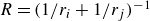 $R=(1/r_i+1/r_j)^{-1}$
is the effective radius, and
$R=(1/r_i+1/r_j)^{-1}$
is the effective radius, and
 $E=((1-\nu _{p,i}^2/E_i) + (1-\nu _{p,j}^2/E_j))^{-1}$
is the effective elastic modulus and
$E=((1-\nu _{p,i}^2/E_i) + (1-\nu _{p,j}^2/E_j))^{-1}$
is the effective elastic modulus and
 $r_i$
,
$r_i$
,
 $E_i$
and
$E_i$
and
 $\nu _{p,i}$
are the radius, Young’s modulus and the Poisson ratio of particle
$\nu _{p,i}$
are the radius, Young’s modulus and the Poisson ratio of particle
 $i$
, respectively. The tangent force
$i$
, respectively. The tangent force
 $F_t$
is determined from the static friction model with the friction coefficient
$F_t$
is determined from the static friction model with the friction coefficient
 $\mu _t =0.3$
chosen based on experimental measurements (Thornton & Yin Reference Thornton and Yin1991). The associated torque is then determined as
$\mu _t =0.3$
chosen based on experimental measurements (Thornton & Yin Reference Thornton and Yin1991). The associated torque is then determined as
 \begin{equation} \mathbf{T}_{i \leftarrow j}^C = \mathbf{r}_{C,ij} \times (F_t \mathbf{t}). \end{equation}
Here,
 $\mathbf{r}_{C,ij}$
points from the centre of particle
$\mathbf{r}_{C,ij}$
points from the centre of particle
 $i$
to the contact point between
$i$
to the contact point between
 $i$
and
$i$
and
 $j$
. Once the collision force and torque from each contact neighbour
$j$
. Once the collision force and torque from each contact neighbour
 $j$
is computed, the total collision force and torque in (2.3) can be obtained as
$j$
is computed, the total collision force and torque in (2.3) can be obtained as
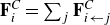 $\mathbf{F}_i^C = \sum _j \mathbf{F}^C_{i \leftarrow j}$
and
$\mathbf{F}_i^C = \sum _j \mathbf{F}^C_{i \leftarrow j}$
and
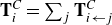 $\mathbf{T}_i^C = \sum _j \mathbf{T}^C_{i \leftarrow j}$
. Note that the collision interactions between a particle and a wall can be computed similarly by treating the wall as a particle at rest with infinite radius and mass.
$\mathbf{T}_i^C = \sum _j \mathbf{T}^C_{i \leftarrow j}$
. Note that the collision interactions between a particle and a wall can be computed similarly by treating the wall as a particle at rest with infinite radius and mass.
2.5. Validation of neutral particle-laden simulations
Several cases presented in figure 14 of Johnson et al. (Reference Johnson, Bassenne and Moin2020) are selected as benchmark results to validate our solvers for the particle-laden turbulent flows. The key parameters for these cases are summarised in table 3.
Parameters in validation cases.
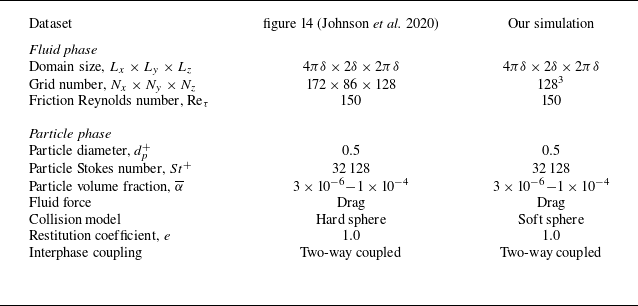
In the reference, a standard two-way coupled Eulerian–Lagrangian framework is employed to simulate the turbophoresis of small inertial particles in a turbulent channel flow. The channel flow is resolved using a grid number of
 $172 \times 86 \times 128$
, and the friction Reynolds number is
$172 \times 86 \times 128$
, and the friction Reynolds number is
 $\textrm{Re}_{\tau }=150$
. Neutral solid particles are subject to fluid drag force, while interparticle collisions are modelled using a hard-sphere model. A restitution coefficient of
$\textrm{Re}_{\tau }=150$
. Neutral solid particles are subject to fluid drag force, while interparticle collisions are modelled using a hard-sphere model. A restitution coefficient of
 $e=1.0$
is used, indicating that collisions are purely elastic. The effects of two-way coupling are also accounted for.
$e=1.0$
is used, indicating that collisions are purely elastic. The effects of two-way coupling are also accounted for.
In our simulation, both the domain size and the Reynolds number are chosen to match those in the reference, while the grid resolution of
 $128^3$
is consistent with that introduced in § 2.2. In the reference, simulations were conducted for four different Stokes numbers (
$128^3$
is consistent with that introduced in § 2.2. In the reference, simulations were conducted for four different Stokes numbers (
 $St^+=1, 32, 128, 512$
). However, we validate the results only for
$St^+=1, 32, 128, 512$
). However, we validate the results only for
 $St^+=32$
and
$St^+=32$
and
 $128$
, as these values are more relevant to the particle inertia discussed in this study. The particle diameter is fixed at
$128$
, as these values are more relevant to the particle inertia discussed in this study. The particle diameter is fixed at
 ${d}_p=0.5 \delta _\nu$
, and the particle densities are set to
${d}_p=0.5 \delta _\nu$
, and the particle densities are set to
 $\rho _p = 2765 \ {\textrm{kg m}^{-3}}$
(
$\rho _p = 2765 \ {\textrm{kg m}^{-3}}$
(
 $St^+=32$
) and
$St^+=32$
) and
 $ 11\,059 \ {\textrm{kg m}^{-3}}$
(
$ 11\,059 \ {\textrm{kg m}^{-3}}$
(
 $St^+=128$
) to achieve the desired Stokes number. The numbers of particles in the simulations vary according to different particle volume fractions:
$St^+=128$
) to achieve the desired Stokes number. The numbers of particles in the simulations vary according to different particle volume fractions:
 $N_p=24429$
(
$N_p=24429$
(
 $\overline {\alpha }_p=3 \times 10^{-6}$
),
$\overline {\alpha }_p=3 \times 10^{-6}$
),
 $N_p=81\,430$
(
$N_p=81\,430$
(
 $\overline {\alpha }_p=1 \times 10^{-5}$
),
$\overline {\alpha }_p=1 \times 10^{-5}$
),
 $N_p=2\,44\,290$
(
$N_p=2\,44\,290$
(
 $\overline {\alpha }_p=3 \times 10^{-5}$
),
$\overline {\alpha }_p=3 \times 10^{-5}$
),
 $N_p=8\,14\,300$
(
$N_p=8\,14\,300$
(
 $\overline {\alpha }_p=1 \times 10^{-4}$
). The drag force is computed as described in § 2.4.1, while the normal collision force is resolved using the soft-sphere Hertzian contact model (§ 2.4.2), assuming that collisions are elastic. Finally, interphase coupling is incorporated following the approach mentioned in § 2.4.1.
$\overline {\alpha }_p=1 \times 10^{-4}$
). The drag force is computed as described in § 2.4.1, while the normal collision force is resolved using the soft-sphere Hertzian contact model (§ 2.4.2), assuming that collisions are elastic. Finally, interphase coupling is incorporated following the approach mentioned in § 2.4.1.
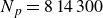
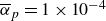
Steady wall-normal particle concentration
 $C/C_0$
for particles with (a)
$C/C_0$
for particles with (a)
 $St^+=32$
and (b)
$St^+=32$
and (b)
 $St^+=128$
. Circles (
$St^+=128$
. Circles (
 $\circ$
) denote profiles obtained from Johnson et al. (Reference Johnson, Bassenne and Moin2020), while plus signs (
$\circ$
) denote profiles obtained from Johnson et al. (Reference Johnson, Bassenne and Moin2020), while plus signs (
 $+$
) represent simulation results using the methods introduced in this study.
$+$
) represent simulation results using the methods introduced in this study.
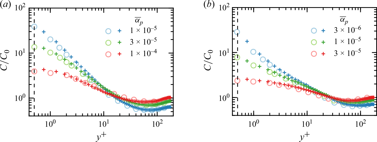
Figure 4 compares the wall-normal particle concentration profiles in the steady state. The vertical dashed line (
 $y^+=0.5$
) marks the location where particles collide with the wall. The profiles corresponding to different
$y^+=0.5$
) marks the location where particles collide with the wall. The profiles corresponding to different
 $St^+$
and
$St^+$
and
 $\overline {\alpha }_p$
show reasonable agreement, demonstrating the reliability of both the fluid and particle solvers.
$\overline {\alpha }_p$
show reasonable agreement, demonstrating the reliability of both the fluid and particle solvers.
2.6. Electrostatic interaction
2.6.1. Particle–particle–particle–mesh method
The particle–particle–particle–mesh method (P
 $^3$
M) is employed to calculate the Eulerian electric field and to resolve the electrostatic interaction acting on charged particles (Yao & Capecelatro Reference Yao and Capecelatro2018; Hockney & Eastwood Reference Hockney and Eastwood2021). The particle charges are assumed as point charges located at particle centres, and the electrostatic force acting on particle
$^3$
M) is employed to calculate the Eulerian electric field and to resolve the electrostatic interaction acting on charged particles (Yao & Capecelatro Reference Yao and Capecelatro2018; Hockney & Eastwood Reference Hockney and Eastwood2021). The particle charges are assumed as point charges located at particle centres, and the electrostatic force acting on particle
 $i$
is
$i$
is
 \begin{equation} \mathbf{F}_{i}^E = q_i \mathbf{E}(\mathbf{x}_i), \end{equation}
where
 $q_i$
is the particle charge and
$q_i$
is the particle charge and
 $\mathbf{E}(\mathbf{x}_i)$
is the electric field at the particle location
$\mathbf{E}(\mathbf{x}_i)$
is the electric field at the particle location
 $\mathbf{x}_i$
. The idea of P
$\mathbf{x}_i$
. The idea of P
 $^3$
M is to split the electrostatic field into two parts
$^3$
M is to split the electrostatic field into two parts
 \begin{equation} \mathbf{E}(\mathbf{x}_i)=\mathbf{E}_M(\mathbf{x}_i)+\mathbf{E}_C (\mathbf{x}_i). \end{equation}
Here,
 $\mathbf{E}_M (\mathbf{x}_i)$
is the long-range contribution that can be efficiently obtained from the Eulerian electric field, while
$\mathbf{E}_M (\mathbf{x}_i)$
is the long-range contribution that can be efficiently obtained from the Eulerian electric field, while
 $\mathbf{E}_C (\mathbf{x}_i)$
is the short-range correction that only needs to be included when other particles are within a critical distance
$\mathbf{E}_C (\mathbf{x}_i)$
is the short-range correction that only needs to be included when other particles are within a critical distance
 $r_{cut}$
to the target particle.
$r_{cut}$
to the target particle.
To find the long-range contribution
 $\mathbf{E}_M (\mathbf{x}_i)$
, the point charges
$\mathbf{E}_M (\mathbf{x}_i)$
, the point charges
 $q_j$
carried by discrete particles located at
$q_j$
carried by discrete particles located at
 $\mathbf{x}_j$
are first filtered and sent to the Cartesian mesh. The resulting volumetric charge density
$\mathbf{x}_j$
are first filtered and sent to the Cartesian mesh. The resulting volumetric charge density
 $\rho _M$
on the mesh is
$\rho _M$
on the mesh is
 \begin{equation} \rho _M (\mathbf{X}_i) = \frac {1}{V_{cell,i}}\sum _{j} q_j G_E(|\mathbf{X}_i-\mathbf{x}_j|), \end{equation}
where the electric Gaussian filter is
 \begin{equation} G_E(\mathbf{r})=\frac {\beta ^3}{\pi ^{3/2}} e^{-\beta ^2 |\mathbf{r}|^2}. \end{equation}
The width of the Gaussian filter at the half-height is related to
 $\beta$
by
$\beta$
by
 $\delta _E=2\sqrt {2\ln {2}}/ \beta$
. The electric Poisson equation (2.16a
) is discretised to the second-order spatial accuracy, and is solved for the electric potential
$\delta _E=2\sqrt {2\ln {2}}/ \beta$
. The electric Poisson equation (2.16a
) is discretised to the second-order spatial accuracy, and is solved for the electric potential
 $\phi _M$
using the same method as that for the pressure Poisson equation in § 2.3. The electric field (
$\phi _M$
using the same method as that for the pressure Poisson equation in § 2.3. The electric field (
 $\mathbf{E}_M$
) is then determined by (2.16b
) with the fourth-order central differencing scheme. Finally, the electric field at the particle locations (
$\mathbf{E}_M$
) is then determined by (2.16b
) with the fourth-order central differencing scheme. Finally, the electric field at the particle locations (
 $\mathbf{E}_M (\mathbf{x}_i)$
) is further interpolated using the fourth-order Lagrange interpolation
$\mathbf{E}_M (\mathbf{x}_i)$
) is further interpolated using the fourth-order Lagrange interpolation
 \begin{equation} \boldsymbol{\nabla} ^2 \phi _{\textrm{M}} = -\frac {\rho _M}{\epsilon _0}, \end{equation}
 \begin{equation} \mathbf{E}_M=-\boldsymbol{\nabla} \phi _M. \end{equation}
For a particle
 $j$
at
$j$
at
 $\mathbf{x}_j$
that is close to the target particle
$\mathbf{x}_j$
that is close to the target particle
 $i$
at
$i$
at
 $\mathbf{x}_i$
, the filtered field contribution using (2.14) to (2.16b
) is
$\mathbf{x}_i$
, the filtered field contribution using (2.14) to (2.16b
) is
 \begin{equation} \mathbf{E}_{M,ij} = \frac {q_j \mathbf{r}_{ij}}{4 \pi \varepsilon _0 |\mathbf{r}_{ij}|^3} \left [ 1- \textrm{erfc} \left (\beta |\mathbf{r}_{ij}|\right ) - \frac {2 \beta |\mathbf{r}_{ij}|}{\sqrt {\pi }}\textrm{exp} \left (-\beta ^2 |\mathbf{r}_{ij}|^2 \right ) \right ], \end{equation}
where
 $\mathbf{r}_{ij} = \mathbf{x}_i-\mathbf{x}_j$
is the vector pointing from
$\mathbf{r}_{ij} = \mathbf{x}_i-\mathbf{x}_j$
is the vector pointing from
 $\mathbf{x}_j$
to
$\mathbf{x}_j$
to
 $\mathbf{x}_i$
, and erfc is the complimentary error function. Meanwhile, the exact contribution should be
$\mathbf{x}_i$
, and erfc is the complimentary error function. Meanwhile, the exact contribution should be
 \begin{equation} \mathbf{E}_{exact,ij} = \frac {q_j \mathbf{r}_{ij}}{4 \pi \varepsilon _0 |\mathbf{r}_{ij}|^3}. \end{equation}
To eliminate the error due to filtering, the short-range correction is added if the interparticle distance is within the cutoff distance
 $r_{cut}$
as
$r_{cut}$
as
 \begin{equation} \begin{aligned} \mathbf{E}_C (\mathbf{x}_i) & = \sum _{ \substack {j \neq i \\ |\mathbf{r}_{ij}|\lt r_{cut}} } \left ( \mathbf{E}_{exact,ij} - \mathbf{E}_{M,ij} \right ) \\ & = \sum _{\substack {j \neq i \\ |\mathbf{r}_{ij}|\lt r_{cut}}} \frac {q_j \mathbf{r}_{ij}}{4 \pi \varepsilon _0 |\mathbf{r}_{ij}|^3} \left [ \textrm{erfc} \left (\beta |\mathbf{r}_{ij}|\right ) + \frac {2 \beta |\mathbf{r}_{ij}|}{\sqrt {\pi }} \textrm{exp}\left (-\beta ^2 |\mathbf{r}_{ij}|^2 \right ) \right ]. \end{aligned} \end{equation}
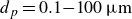
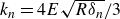
Schematic of the P
 $^3$
M validation: (a) positive/negative (red/blue) point charges carried by particles, (b) the normalised charging density
$^3$
M validation: (a) positive/negative (red/blue) point charges carried by particles, (b) the normalised charging density
 $\rho _M / (q N_p/L^3)$
and (c) the normalised electric potential
$\rho _M / (q N_p/L^3)$
and (c) the normalised electric potential
 $\phi _M / (q N_p/4 \pi L)$
in a thin slice. (d) Dependence of the relative error
$\phi _M / (q N_p/4 \pi L)$
in a thin slice. (d) Dependence of the relative error
 $\epsilon _r$
(2.20) of P
$\epsilon _r$
(2.20) of P
 $^3$
M method on the parameter
$^3$
M method on the parameter
 $\beta$
. (e) Dirichlet boundary conditions at the wall (
$\beta$
. (e) Dirichlet boundary conditions at the wall (
 $\phi _w=0$
) and the added image particles.
$\phi _w=0$
) and the added image particles.
To validate the accuracy of the P
 $^3$
M method, the electrostatic forces calculated from both the P
$^3$
M method, the electrostatic forces calculated from both the P
 $^3$
M method and the standard Ewald summation (Deserno & Holm Reference Deserno and Holm1998) are compared. Details about the Ewald summation are introduced in Appendix F. In the test case,
$^3$
M method and the standard Ewald summation (Deserno & Holm Reference Deserno and Holm1998) are compared. Details about the Ewald summation are introduced in Appendix F. In the test case,
 $N_p=5000$
particles are randomly placed in a triply periodic domain with the side length
$N_p=5000$
particles are randomly placed in a triply periodic domain with the side length
 $L=2\pi$
. Half of the particles carry a nominal positive charge
$L=2\pi$
. Half of the particles carry a nominal positive charge
 $q=1$
while the others carry a nominal negative charge
$q=1$
while the others carry a nominal negative charge
 $q=-1$
(figure 5
a–c). When implementing P
$q=-1$
(figure 5
a–c). When implementing P
 $^3$
M, the Cartesian grid number is set to
$^3$
M, the Cartesian grid number is set to
 $128^3$
. The cutoff distance is fixed at
$128^3$
. The cutoff distance is fixed at
 $r_{cut}=0.2$
for the following reasons. First,
$r_{cut}=0.2$
for the following reasons. First,
 $r_{cut}$
needs to be sufficiently large to ensure the convergence of short-range corrections for all particles. At the same time,
$r_{cut}$
needs to be sufficiently large to ensure the convergence of short-range corrections for all particles. At the same time,
 $r_{cut}$
cannot be too large, as this would significantly increase computational cost. In the test case, for a fixed
$r_{cut}$
cannot be too large, as this would significantly increase computational cost. In the test case, for a fixed
 $\beta$
,
$\beta$
,
 $r_{cut}$
is gradually increased, and the normal of the residual electrostatic force,
$r_{cut}$
is gradually increased, and the normal of the residual electrostatic force,
 $|\mathbf{F}^E-\mathbf{F}^{E,Ewald}|$
(the numerator in (2.20)), is calculated. As
$|\mathbf{F}^E-\mathbf{F}^{E,Ewald}|$
(the numerator in (2.20)), is calculated. As
 $r_{cut}$
increases, the residual force continues to decrease and approaches a minimum at around
$r_{cut}$
increases, the residual force continues to decrease and approaches a minimum at around
 $r_{cut}=0.2$
. Based on this result,
$r_{cut}=0.2$
. Based on this result,
 $r_{cut}=0.2$
is selected for the test, which ensures both force convergence and computational efficiency. The value of
$r_{cut}=0.2$
is selected for the test, which ensures both force convergence and computational efficiency. The value of
 $\beta$
is then swept to change the electric filter length
$\beta$
is then swept to change the electric filter length
 $\delta _E$
. The P
$\delta _E$
. The P
 $^3$
M results are denoted by
$^3$
M results are denoted by
 $\mathbf{F}_i^E$
, and the relative error
$\mathbf{F}_i^E$
, and the relative error
 $\epsilon _r$
is calculated by
$\epsilon _r$
is calculated by
 \begin{equation} \epsilon _r = \frac {|\boldsymbol {F}^E-\boldsymbol {F}^{E,Ewald}|}{|\boldsymbol {F}^{E,Ewald}|} =\frac {[ \sum _{i=1}^{N_{\textrm{p}}} (\boldsymbol {F}_i^E-\boldsymbol {F}_i^{E,Ewald})^2 /N_{\textrm{p}}]^{1/2}}{[ \sum _{i=1}^{N_{\textrm{p}}} (\boldsymbol {F}_i^{E,Ewald})^2 /N_{\textrm{p}}]^{1/2}}. \end{equation}
The dependence of
 $\epsilon _r$
on
$\epsilon _r$
on
 $\beta$
is shown in figure 5(d). The relative error reaches the minimum
$\beta$
is shown in figure 5(d). The relative error reaches the minimum
 $\epsilon _r=0.88\,\%$
at
$\epsilon _r=0.88\,\%$
at
 $\beta =6.0$
, thus verifying the reliability of the P
$\beta =6.0$
, thus verifying the reliability of the P
 $^3$
M method.
$^3$
M method.
2.6.2. Electrical boundary conditions
In the channel, both the top and bottom boundaries are assumed to be grounded conductive walls. When solving the electric Poisson equation (2.16a
), periodic boundary conditions are applied in the streamwise (
 $x$
) and the spanwise (
$x$
) and the spanwise (
 $z$
) directions, and zero-Dirichlet boundary conditions are added at both walls (
$z$
) directions, and zero-Dirichlet boundary conditions are added at both walls (
 $y=\pm \delta$
)
$y=\pm \delta$
)
 \begin{equation} \phi _w=0. \end{equation}
Note that (2.21) only ensures an appropriate electrical boundary condition on the mesh. When charged particles are close to the wall, the length scale of the local electric field is usually much smaller than the cell size and cannot be fully resolved. Therefore, image particles are added to consider such near-wall effects (Liu et al. 2010; Yao & Capecelatro Reference Yao and Capecelatro2021). If the distance between a particle
 $i$
and the wall is smaller than
$i$
and the wall is smaller than
 $r_{cut}$
, its image is added at the symmetric location
$r_{cut}$
, its image is added at the symmetric location
 $\mathbf{x}_i^{(Im)}$
about the wall with opposite polarity
$\mathbf{x}_i^{(Im)}$
about the wall with opposite polarity
 $q_i^{(Im)}=-q_i$
. When summing the short-range correction force in (2.19), the contribution of all the image particles within
$q_i^{(Im)}=-q_i$
. When summing the short-range correction force in (2.19), the contribution of all the image particles within
 $r_{cut}$
is also added (figure 5
e)
$r_{cut}$
is also added (figure 5
e)
 \begin{equation} \mathbf{E}_C^{(Im)}(\mathbf{x}_i) = \sum _{|\mathbf{r}_{ij}^{(Im)}|\lt r_{cut}} \frac {q_j^{(Im)} \mathbf{r}_{ij}^{(Im)}}{4 \pi \varepsilon _0 |\mathbf{r}_{ij}^{(Im)}|^3} \left [ \textrm{erfc} \left (\beta |\mathbf{r}_{ij}^{(Im)}|\right ) + \frac {2 \beta |\mathbf{r}_{ij}^{(Im)}|}{\sqrt {\pi }} \textrm{exp}\left (-\beta ^2 |\mathbf{r}_{ij}^{(Im)}|^2 \right ) \right ]. \end{equation}
Here,
 $\mathbf{r}_{ij}^{(Im)}$
points from the image of particle
$\mathbf{r}_{ij}^{(Im)}$
points from the image of particle
 $j$
to the target particle
$j$
to the target particle
 $i$
. Therefore, the near-wall correction can be taken as a special case of the short-range correction (2.19) due to all the images.
$i$
. Therefore, the near-wall correction can be taken as a special case of the short-range correction (2.19) due to all the images.
Furthermore, to avoid over-filtering the electric field, the electric filter length is chosen to be
 $\delta _E=5 \delta _\nu$
in the simulations. The cutoff distance
$\delta _E=5 \delta _\nu$
in the simulations. The cutoff distance
 $r_{cut}=36 \delta _\nu$
is set larger than
$r_{cut}=36 \delta _\nu$
is set larger than
 $\delta _E$
so that the short-range correction is converged.
$\delta _E$
so that the short-range correction is converged.
We now note that, using P
 $^3$
M, the accuracy of the PW electrostatic force is inherently equivalent to that of the PP electrostatic force. When evaluating the electric field
$^3$
M, the accuracy of the PW electrostatic force is inherently equivalent to that of the PP electrostatic force. When evaluating the electric field
 $\mathbf{E}(\mathbf{x}_i)$
at the particle locations in a wall-bounded domain, the conducting wall can influence both the long-range contribution,
$\mathbf{E}(\mathbf{x}_i)$
at the particle locations in a wall-bounded domain, the conducting wall can influence both the long-range contribution,
 $\mathbf{E}_M(\mathbf{x}_i)$
, and the short-range correction,
$\mathbf{E}_M(\mathbf{x}_i)$
, and the short-range correction,
 $\mathbf{E}_C(\mathbf{x}_i)$
. First, the electric Poisson equation is solved using periodic boundary conditions in the
$\mathbf{E}_C(\mathbf{x}_i)$
. First, the electric Poisson equation is solved using periodic boundary conditions in the
 $x$
and
$x$
and
 $z$
directions, and a zero-Dirichlet boundary condition (
$z$
directions, and a zero-Dirichlet boundary condition (
 $\phi _w=0$
) at the walls. Since the same Poisson solver is employed with an identical tolerance of
$\phi _w=0$
) at the walls. Since the same Poisson solver is employed with an identical tolerance of
 $\epsilon _{tol}=10^{-6}$
, the accuracy of the electric field on the mesh,
$\epsilon _{tol}=10^{-6}$
, the accuracy of the electric field on the mesh,
 $\mathbf{E}_M$
, in the wall-bounded case is comparable to that in the triply periodic case. The electric field at particle locations is then interpolated using the same fourth-order Lagrangian interpolation, ensuring that the long-range contribution,
$\mathbf{E}_M$
, in the wall-bounded case is comparable to that in the triply periodic case. The electric field at particle locations is then interpolated using the same fourth-order Lagrangian interpolation, ensuring that the long-range contribution,
 $\mathbf{E}_M(\mathbf{x}_i)$
, remains equally accurate in the channel. For the short-range contribution from image particles, the short-range correction for image particles (2.22) has the same functional form as that for real particles (2.19). The only difference lies in the positions and charges of the image particles. Therefore, when summing the short-range corrections within the same cutoff distance,
$\mathbf{E}_M(\mathbf{x}_i)$
, remains equally accurate in the channel. For the short-range contribution from image particles, the short-range correction for image particles (2.22) has the same functional form as that for real particles (2.19). The only difference lies in the positions and charges of the image particles. Therefore, when summing the short-range corrections within the same cutoff distance,
 $r_{cut}$
, contributions from both real and image particles are calculated together. This approach guarantees that the accuracy of
$r_{cut}$
, contributions from both real and image particles are calculated together. This approach guarantees that the accuracy of
 $\mathbf{E}_C(\mathbf{x}_i)$
is preserved. Consequently, the accuracy of P
$\mathbf{E}_C(\mathbf{x}_i)$
is preserved. Consequently, the accuracy of P
 $^3$
M in a wall-bounded domain is of the same order as in a triply periodic domain.
$^3$
M in a wall-bounded domain is of the same order as in a triply periodic domain.
3. Results and discussions
3.1. Wall-normal transport and deposition velocity of charged particles
In each case, particles are released into a fully developed turbulent flow with random initial positions and zero velocity. The particle spatial distribution then starts to evolve from the initially random state towards a steady state that is characterised by a high concentration near the wall. To quantify the temporal evolution of the particle phase, the Shannon entropy
 $\mathcal{S}$
is used to describe the non-uniformity of the wall-normal particle distribution (Picano et al. Reference Picano, Sardina and Casciola2009; Sardina et al. Reference Sardina, Schlatter, Brandt, Picano and Casciola2012). It takes approximately
$\mathcal{S}$
is used to describe the non-uniformity of the wall-normal particle distribution (Picano et al. Reference Picano, Sardina and Casciola2009; Sardina et al. Reference Sardina, Schlatter, Brandt, Picano and Casciola2012). It takes approximately
 $(1{-}2) \times 10^4 \tau _{\nu }$
for the particle distribution to transition from the initial random distribution to a steady state, where
$(1{-}2) \times 10^4 \tau _{\nu }$
for the particle distribution to transition from the initial random distribution to a steady state, where
 $\mathcal{S}$
is independent of time (not shown). Statistics are then taken over another
$\mathcal{S}$
is independent of time (not shown). Statistics are then taken over another
 $5 \times 10^3 \tau _{\nu }$
and presented below. However, for the case with moderate inertia (
$5 \times 10^3 \tau _{\nu }$
and presented below. However, for the case with moderate inertia (
 $St^+=32$
) and the highest charge (
$St^+=32$
) and the highest charge (
 $q=1 \times 10^{-14} \ \textrm{C}$
), a steady state was not reached after a simulation period exceeding
$q=1 \times 10^{-14} \ \textrm{C}$
), a steady state was not reached after a simulation period exceeding
 $2 \times 10^4 \tau _{\nu }$
. This case is thus excluded from the current discussion of steady-state statistics.
$2 \times 10^4 \tau _{\nu }$
. This case is thus excluded from the current discussion of steady-state statistics.
Normalised wall-normal particle concentration
 $C/C_0$
for both neutral and charged particles with (a)
$C/C_0$
for both neutral and charged particles with (a)
 $St^+=32$
and (b)
$St^+=32$
and (b)
 $St^+=133$
. Scatters are simulation results and dashed lines are predictions using (3.3). Colours from light to dark represent results for
$St^+=133$
. Scatters are simulation results and dashed lines are predictions using (3.3). Colours from light to dark represent results for
 $q=0 \ \textrm{C}$
,
$q=0 \ \textrm{C}$
,
 $5 \times 10^{-15} \ \textrm{C}$
and
$5 \times 10^{-15} \ \textrm{C}$
and
 $1 \times 10^{-14} \ \textrm{C}$
.
$1 \times 10^{-14} \ \textrm{C}$
.
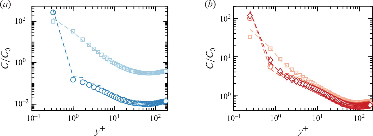
We start with the distribution of charged particles in the wall-normal direction. Figure 6 compares the normalised wall-normal particle concentration
 $C/C_0$
between neutral and charged particles. The local particle concentration
$C/C_0$
between neutral and charged particles. The local particle concentration
 $C(y)$
is equal to the number of particles in each wall-normal bin divided by the bin volume, and the average concentration is
$C(y)$
is equal to the number of particles in each wall-normal bin divided by the bin volume, and the average concentration is
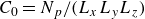 $C_0=N_p/(L_x L_y L_z)$
. In figure 6, the simulation results are represented by scatters, while the dashed lines are model predictions based on (3.3) that will be further detailed in § 3.2. In the neutral cases, particles driven by turbophoresis migrate from the outer layer towards the wall, leading to the increase of
$C_0=N_p/(L_x L_y L_z)$
. In figure 6, the simulation results are represented by scatters, while the dashed lines are model predictions based on (3.3) that will be further detailed in § 3.2. In the neutral cases, particles driven by turbophoresis migrate from the outer layer towards the wall, leading to the increase of
 $C(y)$
as
$C(y)$
as
 $y^+$
decreases. Compared with the more inertial particles with
$y^+$
decreases. Compared with the more inertial particles with
 $St^+=133$
, particles with
$St^+=133$
, particles with
 $St^+=32$
show more pronounced accumulation (
$St^+=32$
show more pronounced accumulation (
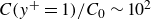 $C(y^+=1)/C_0 \sim 10^2$
) in the neutral case as these particles are more responsive to near-wall coherent structures.
$C(y^+=1)/C_0 \sim 10^2$
) in the neutral case as these particles are more responsive to near-wall coherent structures.
Once particles are charged, the image force further attracts particles towards the walls leading to more significant accumulation. As shown in figure 6(a), most particles with
 $St^+=32$
and
$St^+=32$
and
 $q=5 \times 10^{-15} \ \textrm{C}$
remain concentrated in the innermost bin within the viscous layer, while their concentration in both the buffer layer and the outer layer is drastically reduced. A similar trend is observed for particles with
$q=5 \times 10^{-15} \ \textrm{C}$
remain concentrated in the innermost bin within the viscous layer, while their concentration in both the buffer layer and the outer layer is drastically reduced. A similar trend is observed for particles with
 $St^+=133$
, although to a lesser extent due to their larger inertia. For
$St^+=133$
, although to a lesser extent due to their larger inertia. For
 $St^+=133$
, the normalised concentration at the innermost cell increases from
$St^+=133$
, the normalised concentration at the innermost cell increases from
 $C/C_0=33$
in the neutral case to
$C/C_0=33$
in the neutral case to
 $C/C_0=101$
for
$C/C_0=101$
for
 $q=5 \times 10^{-15} \ \textrm{C}$
and
$q=5 \times 10^{-15} \ \textrm{C}$
and
 $C/C_0=118$
for
$C/C_0=118$
for
 $q=1 \times 10^{-14} \ \textrm{C}$
.
$q=1 \times 10^{-14} \ \textrm{C}$
.
Normalised mean velocity for (a) approaching particles with
 $St^+=32$
, (b) departing particles with
$St^+=32$
, (b) departing particles with
 $St^+=32$
, (c) approaching particles with
$St^+=32$
, (c) approaching particles with
 $St^+=133$
and (d) departing particles with
$St^+=133$
and (d) departing particles with
 $St^+=133$
. Colours from light to dark represent results for
$St^+=133$
. Colours from light to dark represent results for
 $q=0 \ \textrm{C}$
,
$q=0 \ \textrm{C}$
,
 $5 \times 10^{-15} \ \textrm{C}$
and
$5 \times 10^{-15} \ \textrm{C}$
and
 $1 \times 10^{-14} \ \textrm{C}$
.
$1 \times 10^{-14} \ \textrm{C}$
.
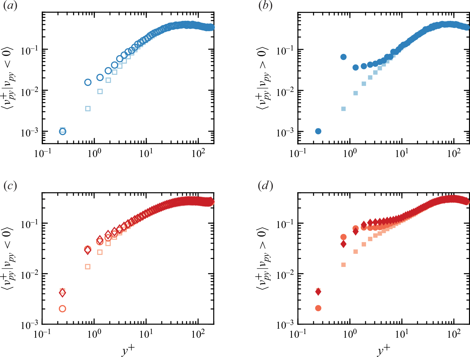
Apart from particle concentration, the mean approaching/departing velocity of particles is also of interest, as it describes how quickly particles located at a given
 $y^+$
move towards or away from the wall. Here, we define the direction pointing away from the wall as the positive direction, so the mean approaching and departing velocities normalised by
$y^+$
move towards or away from the wall. Here, we define the direction pointing away from the wall as the positive direction, so the mean approaching and departing velocities normalised by
 $u_\tau$
are computed as
$u_\tau$
are computed as
 $\langle v^+_{py} |v_{py} \lt 0 \rangle$
and
$\langle v^+_{py} |v_{py} \lt 0 \rangle$
and
 $\langle v^+_{py} |v_{py} \gt 0 \rangle$
, respectively.
$\langle v^+_{py} |v_{py} \gt 0 \rangle$
, respectively.
Figures 7(a) and 7(c) shows the approaching velocity for
 $St^+=32$
and
$St^+=32$
and
 $St^+=133$
. When particles are close to the channel centre, the electrostatic forces pointing towards both walls cancel out, so the approaching velocity for charged particles collapses with that of neutral ones. As particles get closer to the walls, they are accelerated by the electrostatic force towards the closer wall, and the approaching velocity becomes higher than the neutral cases. The increase of the approaching velocity becomes more significant as
$St^+=133$
. When particles are close to the channel centre, the electrostatic forces pointing towards both walls cancel out, so the approaching velocity for charged particles collapses with that of neutral ones. As particles get closer to the walls, they are accelerated by the electrostatic force towards the closer wall, and the approaching velocity becomes higher than the neutral cases. The increase of the approaching velocity becomes more significant as
 $y^+$
decreases, indicating the more significant role played by the electrostatic force in the near-wall region.
$y^+$
decreases, indicating the more significant role played by the electrostatic force in the near-wall region.
However, the approaching velocity at the walls (the leftmost points in figures 7
a and 7
c) is smaller than the neutral velocity for both
 $St^+$
. This can be attributed to several reasons. First, the two-way coupling effect caused by the concentrated particles near the wall could effectively weaken local flows, thereby reducing the wall-normal particle velocity. Although the domain-averaged particle volume fraction is as low as
$St^+$
. This can be attributed to several reasons. First, the two-way coupling effect caused by the concentrated particles near the wall could effectively weaken local flows, thereby reducing the wall-normal particle velocity. Although the domain-averaged particle volume fraction is as low as
 $\overline {\alpha } \sim O(10^{-6})$
, the near-wall particle volume fraction is more than two orders of magnitude higher (figure 6), which is sufficient to modulate the near-wall local flows (Elghobashi Reference Elghobashi1994; Balachandar & Eaton Reference Balachandar and Eaton2010). Besides, after bouncing off the wall, particles must overcome the electrostatic force to become re-entrained into the outer layer. Consequently, more charged particles are trapped in the viscous layer and adjust to the low fluid velocity. Meanwhile, high-speed particles are energetic enough to escape and become re-entrained. This biased sampling of high-speed particles leads to the increase in the mean departing velocity in figures 7(b) and 7(d).
$\overline {\alpha } \sim O(10^{-6})$
, the near-wall particle volume fraction is more than two orders of magnitude higher (figure 6), which is sufficient to modulate the near-wall local flows (Elghobashi Reference Elghobashi1994; Balachandar & Eaton Reference Balachandar and Eaton2010). Besides, after bouncing off the wall, particles must overcome the electrostatic force to become re-entrained into the outer layer. Consequently, more charged particles are trapped in the viscous layer and adjust to the low fluid velocity. Meanwhile, high-speed particles are energetic enough to escape and become re-entrained. This biased sampling of high-speed particles leads to the increase in the mean departing velocity in figures 7(b) and 7(d).
With both particle concentration and wall-normal velocity, we can define the wall-normal particle flux
 $k$
, which measures the number of particles crossing a wall-parallel plane per unit time per unit area. The wall-normal particle flux towards (
$k$
, which measures the number of particles crossing a wall-parallel plane per unit time per unit area. The wall-normal particle flux towards (
 $-$
) and away from the wall (
$-$
) and away from the wall (
 $+$
) can be given by
$+$
) can be given by
 \begin{equation} k^{(-)}(y)= \langle v_{py} |v_{py}\lt 0 \rangle (y) \cdot C(y) \cdot P(v_{py}\lt 0|y), \end{equation}
 \begin{equation} k^{(+)}(y)= \langle v_{py} |v_{py}\gt 0 \rangle (y) \cdot C(y) \cdot P(v_{py}\gt 0|y). \end{equation}
Here,
 $P(v_{py}\lt 0|y)$
and
$P(v_{py}\lt 0|y)$
and
 $P(v_{py}\gt 0|y)$
are the proportions of particles moving towards and away from the walls at
$P(v_{py}\gt 0|y)$
are the proportions of particles moving towards and away from the walls at
 $y$
. Note that, after normalising the particle flux
$y$
. Note that, after normalising the particle flux
 $k$
as
$k$
as
 \begin{equation} k^{+,(-)}=\frac {k^{(-)}}{u_\tau C_0}, \ \text{and} \ k^{+,(+)}=\frac {k^{(+)}}{u_\tau C_0}, \end{equation}
the dimensionless particle flux
 $k^+$
has the same physical meaning as the dimensionless deposition velocity defined in other works (Guha Reference Guha2008; Fong et al. Reference Fong, Amili and Coletti2019).
$k^+$
has the same physical meaning as the dimensionless deposition velocity defined in other works (Guha Reference Guha2008; Fong et al. Reference Fong, Amili and Coletti2019).
Figure 8 displays profiles of
 $k^+$
for different
$k^+$
for different
 $St^+$
and
$St^+$
and
 $q$
. For neutral particles, one notices that the dimensionless flux
$q$
. For neutral particles, one notices that the dimensionless flux
 $k^+$
is not constant and shows a similar trend along the
$k^+$
is not constant and shows a similar trend along the
 $y$
direction for both
$y$
direction for both
 $St^+=32$
and
$St^+=32$
and
 $St^+=133$
. This trend is consistent with the particle transport mechanisms described in previous works (Soldati & Marchioli Reference Soldati and Marchioli2009; Chen et al. Reference Chen, Chen, Wu, Ruan and Li2022). Particles in the buffer layer (
$St^+=133$
. This trend is consistent with the particle transport mechanisms described in previous works (Soldati & Marchioli Reference Soldati and Marchioli2009; Chen et al. Reference Chen, Chen, Wu, Ruan and Li2022). Particles in the buffer layer (
 $5 \leqslant y^+ \leqslant 30$
) are swept by quasi-streamwise vortices and obtain a net drift velocity towards the near-wall region, which accounts for the rise of
$5 \leqslant y^+ \leqslant 30$
) are swept by quasi-streamwise vortices and obtain a net drift velocity towards the near-wall region, which accounts for the rise of
 $k^+$
in the buffer layer. Then particles trapped near the wall could either deposit at the wall after decelerating in the viscous layer, or be re-entrained to the outer layer by ejections, both of which will reduce
$k^+$
in the buffer layer. Then particles trapped near the wall could either deposit at the wall after decelerating in the viscous layer, or be re-entrained to the outer layer by ejections, both of which will reduce
 $k^+$
in the viscous layer (
$k^+$
in the viscous layer (
 $ y^+ \leqslant 5$
). Compared with
$ y^+ \leqslant 5$
). Compared with
 $St^+=32$
, particles with
$St^+=32$
, particles with
 $St^+=133$
are more inertial and undergo a weaker deceleration, so
$St^+=133$
are more inertial and undergo a weaker deceleration, so
 $k^+$
is less decreased in the viscous layer. When particles are charged, the electrostatic force becomes more dominant as particles get closer to walls, so
$k^+$
is less decreased in the viscous layer. When particles are charged, the electrostatic force becomes more dominant as particles get closer to walls, so
 $k$
keeps increasing as
$k$
keeps increasing as
 $y^+$
decreases. As most of the charged particles are concentrated near the wall (figure 6), a sharp increase in the near-wall flux and a decrease in the far-field flux are observed.
$y^+$
decreases. As most of the charged particles are concentrated near the wall (figure 6), a sharp increase in the near-wall flux and a decrease in the far-field flux are observed.
Dimensionless particle flux
 $k^+$
for (a)
$k^+$
for (a)
 $St^+=32$
and (b)
$St^+=32$
and (b)
 $St^+=133$
. Circles (
$St^+=133$
. Circles (
 $\circ$
) and plus signs (
$\circ$
) and plus signs (
 $+$
) represent approaching and departing fluxes. The horizontal black dashed lines indicate neutral deposition velocity
$+$
) represent approaching and departing fluxes. The horizontal black dashed lines indicate neutral deposition velocity
 $k_d^+$
. Colours from light to dark represent results for
$k_d^+$
. Colours from light to dark represent results for
 $q=0 \ \textrm{C}$
,
$q=0 \ \textrm{C}$
,
 $5 \times 10^{-15} \ \textrm{C}$
and
$5 \times 10^{-15} \ \textrm{C}$
and
 $1 \times 10^{-14} \ \textrm{C}$
.
$1 \times 10^{-14} \ \textrm{C}$
.

To make a direct comparison with the classic model prediction, it is necessary to define the deposition velocity of the particles. In previous experimental investigations, deposition velocity was obtained by directly measuring the total number (or mass) of droplets or particles deposited onto the wall in each test (Friedlander & Johnstone Reference Friedlander and Johnstone1957; Liu & Agarwal Reference Liu and Agarwal1974). However, in this study, the process of particle sticking and deposition onto the wall is not included. Therefore, a specific wall-normal location
 $y^+$
must be selected, and the dimensionless deposition velocity
$y^+$
must be selected, and the dimensionless deposition velocity
 $k^+_d$
is defined as the local particle flux
$k^+_d$
is defined as the local particle flux
 $k^+(y^+)$
.
$k^+(y^+)$
.
For neutral particles, the deposition velocity at
 $y^+=1$
is chosen (black dashed lines in figure 8) for two reasons. First, dust particles typically have a finite size comparable to the viscous length, making the deposition velocity at
$y^+=1$
is chosen (black dashed lines in figure 8) for two reasons. First, dust particles typically have a finite size comparable to the viscous length, making the deposition velocity at
 $y^+ \sim 1$
, just before particles bounce off, more relevant. Additionally,
$y^+ \sim 1$
, just before particles bounce off, more relevant. Additionally,
 $k^+$
plateaus near
$k^+$
plateaus near
 $y^+=1$
, which represents the maximum rate at which turbulence transports particles towards the wall before they are slowed down in the viscous layer.
$y^+=1$
, which represents the maximum rate at which turbulence transports particles towards the wall before they are slowed down in the viscous layer.
For charged particles, the electrostatic-enhanced accumulation occurs in the innermost cells before particles bounce off. Since the particle size used in the simulation is small, the deposition velocity at the innermost cell is chosen as
 $k^+_d$
. If a larger particle size is used, the flux profiles of charged particles are expected to shift towards larger
$k^+_d$
. If a larger particle size is used, the flux profiles of charged particles are expected to shift towards larger
 $y^+$
, leading to a different deposition velocity. Despite these variations, the change in deposition velocity
$y^+$
, leading to a different deposition velocity. Despite these variations, the change in deposition velocity
 $k^+_d$
due to particle charging is expected to remain consistent.
$k^+_d$
due to particle charging is expected to remain consistent.
The deposition velocities
 $k^+_d$
from simulations are then compared with the predictions using the one-dimensional Eulerian model by Guha (Reference Guha2008) in figure 9. In the reference, the particle charge is measured by the charging parameter
$k^+_d$
from simulations are then compared with the predictions using the one-dimensional Eulerian model by Guha (Reference Guha2008) in figure 9. In the reference, the particle charge is measured by the charging parameter
 $\xi =q/q_{max}$
with the max particle charge
$\xi =q/q_{max}$
with the max particle charge
 $q_{max}$
depending on the particle size. Plugging in the parameters from table 2 then leads to
$q_{max}$
depending on the particle size. Plugging in the parameters from table 2 then leads to
 $\xi =0.16$
for
$\xi =0.16$
for
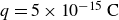 $q=5 \times 10^{-15} \ \textrm{C}$
and
$q=5 \times 10^{-15} \ \textrm{C}$
and
 $\xi =0.31$
for
$\xi =0.31$
for
 $q=1 \times 10^{-14} \ \textrm{C}$
. In the neutral case, the deposition velocities for both
$q=1 \times 10^{-14} \ \textrm{C}$
. In the neutral case, the deposition velocities for both
 $St^+$
are close to the model prediction. However, a discrepancy arises in the charged case. While Guha’s model predicts little difference in the deposition velocity of charged particles with
$St^+$
are close to the model prediction. However, a discrepancy arises in the charged case. While Guha’s model predicts little difference in the deposition velocity of charged particles with
 $St^+ \geqslant 10$
, our simulation results suggest that this may not be the case. Therefore, the physical mechanisms that enhance the deposition velocity of charged particles in the current simulations need to be further examined in the following sections.
$St^+ \geqslant 10$
, our simulation results suggest that this may not be the case. Therefore, the physical mechanisms that enhance the deposition velocity of charged particles in the current simulations need to be further examined in the following sections.
Comparison of deposition velocity
 $k^+_d$
between the current work (scatters) and the model prediction by Guha (Reference Guha2008) (solid lines). Solid lines from light to dark are results from the charging parameter
$k^+_d$
between the current work (scatters) and the model prediction by Guha (Reference Guha2008) (solid lines). Solid lines from light to dark are results from the charging parameter
 $\xi =0$
,
$\xi =0$
,
 $0.05$
,
$0.05$
,
 $0.1$
,
$0.1$
,
 $0.5$
,
$0.5$
,
 $0.75$
, and
$0.75$
, and
 $1$
. Colours from light to dark represent results for
$1$
. Colours from light to dark represent results for
 $q=0 \ \textrm{C}$
(
$q=0 \ \textrm{C}$
(
 $\xi =0$
),
$\xi =0$
),
 $5 \times 10^{-15} \ \textrm{C}$
(
$5 \times 10^{-15} \ \textrm{C}$
(
 $\xi =0.16$
) and
$\xi =0.16$
) and
 $1 \times 10^{-14} \ \textrm{C}$
(
$1 \times 10^{-14} \ \textrm{C}$
(
 $\xi =0.31$
).
$\xi =0.31$
).
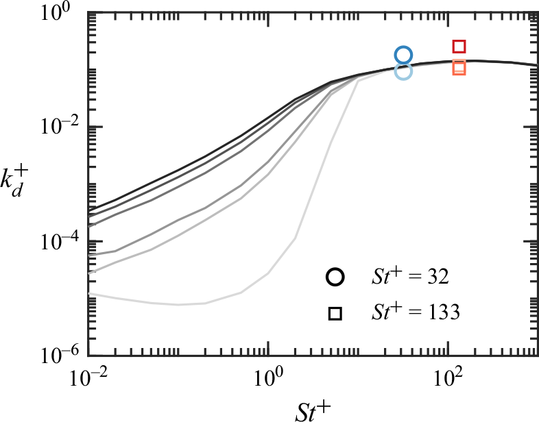
3.2. Driving mechanisms of wall-normal particle accumulation
In the previous section, it has been demonstrated that the electrostatic force increases the deposition velocity for particles with
 $St^+ =32$
and
$St^+ =32$
and
 $St^+=133$
. While both particle concentration (figure 6) and wall-normal velocities (figure 7) are affected, the change in particle concentration is more significant, which makes a predominant contribution to the increased deposition velocity. This finding also confirms that the assumption of an unchanged concentration profile for charged particles in Guha’s model is invalid. In this section, we focus on the changes in particle concentration under the influence of electrostatic forces.
$St^+=133$
. While both particle concentration (figure 6) and wall-normal velocities (figure 7) are affected, the change in particle concentration is more significant, which makes a predominant contribution to the increased deposition velocity. This finding also confirms that the assumption of an unchanged concentration profile for charged particles in Guha’s model is invalid. In this section, we focus on the changes in particle concentration under the influence of electrostatic forces.
To quantify the contributions of different physical mechanics to the wall-normal particle distribution, the statistical approach proposed by Johnson et al. (Reference Johnson, Bassenne and Moin2020) is employed here. This one-dimensional model was originally developed for neutral particles, and has been recently extended to include charged particles (Di Renzo et al. Reference Di Renzo, Johnson, Bassenne, Villafañe and Urzay2019; Zhang et al. Reference Zhang, Cui and Zheng2023a ). For completeness, key aspects of the model are introduced in Appendix G, with further details available in the cited references. When the particle phase reaches equilibrium, the steady concentration profile can be given by
 \begin{equation} C(y)= \mathcal{C}^{\prime } \textrm{exp} (I_{turb} + I_{bias} +I_{elec}). \end{equation}
Three different integrals are defined in the exponent of (3.3)
 \begin{equation} I_{turb}=-\int _0^y \frac {\textrm{d} \ln { \langle v_{py}^2 | \eta \rangle }}{\textrm{d} \eta } \textrm{d} \eta, \end{equation}
 \begin{equation} I_{bias}=\frac {1}{\tau _p} \int _0^y \frac {\langle f_I (u_{fy}-v_{py}) |\eta \rangle }{\langle v_{py}^2 |\eta \rangle } \textrm{d} \eta, \end{equation}
 \begin{equation} I_{elec}=\frac {q}{m} \int _0^y \frac {\langle E_{y} | \eta \rangle }{\langle v_{py}^2 | \eta \rangle } \textrm{d} \eta . \end{equation}
Here,
 $v_{py}$
is the wall-normal particle velocity,
$v_{py}$
is the wall-normal particle velocity,
 $u_{fy}$
is the wall-normal fluid velocity at the particle location,
$u_{fy}$
is the wall-normal fluid velocity at the particle location,
 $f_{I}$
is the Schiller–Naumann correction factor for the drag force and
$f_{I}$
is the Schiller–Naumann correction factor for the drag force and
 $E_y$
is the wall-normal electric field at the particle location.
$E_y$
is the wall-normal electric field at the particle location.
The unknown coefficient
 $\mathcal{C}^{\prime }$
in (3.3) can be determined as follows. In the steady state, we first compute the mean profiles of the wall-normal particle kinetic energy
$\mathcal{C}^{\prime }$
in (3.3) can be determined as follows. In the steady state, we first compute the mean profiles of the wall-normal particle kinetic energy
 $\langle v_{py}^2 \rangle (y)$
, the wall-normal drag force
$\langle v_{py}^2 \rangle (y)$
, the wall-normal drag force
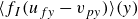 $\langle f_I (u_{fy}-v_{py})\rangle (y)$
and the wall-normal electric field
$\langle f_I (u_{fy}-v_{py})\rangle (y)$
and the wall-normal electric field
 $\langle E_{y}\rangle (y)$
. Then for each cell centre location
$\langle E_{y}\rangle (y)$
. Then for each cell centre location
 $y$
, the integrals
$y$
, the integrals
 $I_{turb}(y)$
,
$I_{turb}(y)$
,
 $I_{bias}(y)$
,
$I_{bias}(y)$
,
 $I_{elec}(y)$
are obtained by integrating the corresponding terms from the innermost cell to the current cell at
$I_{elec}(y)$
are obtained by integrating the corresponding terms from the innermost cell to the current cell at
 $y$
following (3.4). Because of particle mass conservation, the mean particle concentration
$y$
following (3.4). Because of particle mass conservation, the mean particle concentration
 $C_0$
across the channel can be related to the concentration profile
$C_0$
across the channel can be related to the concentration profile
 $C(y)$
by
$C(y)$
by
 \begin{equation} C_0 = \frac {1}{\delta } \int _0^{\delta } C(y) \textrm{d}y = \frac {\mathcal{C}^{\prime }}{\delta } \int _0^{\delta } \textrm{exp} \left ( I_{turb}(y) + I_{bias}(y) +I_{elec}(y) \right ) \textrm{d}y. \end{equation}
In (3.5), both
 $C_0$
and
$C_0$
and
 $\delta$
are constants. By integrating the exponential of the sum of the integrals, the unknown coefficient
$\delta$
are constants. By integrating the exponential of the sum of the integrals, the unknown coefficient
 $\mathcal{C}^{\prime }$
can be determined.
$\mathcal{C}^{\prime }$
can be determined.
Since knowledge of both the particle phase and the fluid phase is required, (3.3) is not capable of predicting the steady concentration profile a priori unless additional model closures are included (Zhang et al. Reference Zhang, Bragg and Wang2023b
). However, these integrals provide insights into the essential roles played by different mechanisms. The first integral
 $I_{turb}$
depends on the gradient of the wall-normal particle kinetic energy and is referred to as the turbophoresis effect. Since
$I_{turb}$
depends on the gradient of the wall-normal particle kinetic energy and is referred to as the turbophoresis effect. Since
 $\langle v_{py}^2 \rangle$
increases as
$\langle v_{py}^2 \rangle$
increases as
 $y$
increases,
$y$
increases,
 $I_{turb}$
is always negative. According to (3.3), the negative
$I_{turb}$
is always negative. According to (3.3), the negative
 $I_{turb}$
reduces
$I_{turb}$
reduces
 $C(y)$
as
$C(y)$
as
 $y$
increases, which means turbophoresis drives particles towards the walls. The second integral
$y$
increases, which means turbophoresis drives particles towards the walls. The second integral
 $I_{bias}$
quantifies the slip velocity experienced by particles, and is referred to as the biased-sampling effect. In a steady state, inertial particles tend to oversample fluids moving away from the wall, leading to a positive slip velocity that pushes particles away from the walls. The last integral
$I_{bias}$
quantifies the slip velocity experienced by particles, and is referred to as the biased-sampling effect. In a steady state, inertial particles tend to oversample fluids moving away from the wall, leading to a positive slip velocity that pushes particles away from the walls. The last integral
 $I_{elec}$
depends on the electrostatic force acting on the charged particles. As will be shown below, the average wall-normal electric field points towards the wall (negative), which consistently attracts particles towards the wall, further contributing to the deposition of charged particles.
$I_{elec}$
depends on the electrostatic force acting on the charged particles. As will be shown below, the average wall-normal electric field points towards the wall (negative), which consistently attracts particles towards the wall, further contributing to the deposition of charged particles.
Comparison of different integrals for particles with (a)
 $St^+=32$
and (b)
$St^+=32$
and (b)
 $St^+=133$
. Colours from light to dark represent results for
$St^+=133$
. Colours from light to dark represent results for
 $q=0 \ \textrm{C}$
,
$q=0 \ \textrm{C}$
,
 $5 \times 10^{-15} \ \textrm{C}$
and
$5 \times 10^{-15} \ \textrm{C}$
and
 $1 \times 10^{-14} \ \textrm{C}$
.
$1 \times 10^{-14} \ \textrm{C}$
.
The wall-normal profiles of the integrals for both neutral and charged particles are displayed in figure 10. By taking the integrals into (3.4) and determining the coefficient
 $\mathcal{C}^{\prime }$
from (3.5), the predicted concentration profiles are plotted in figure 6 as dashed lines, which show good agreement with the simulation results. Equation (3.3) is thus justified and the relative importance of various mechanisms can be directly quantified by comparing the values of the integrals. As shown in figure 10, in the neutral case, the magnitude of
$\mathcal{C}^{\prime }$
from (3.5), the predicted concentration profiles are plotted in figure 6 as dashed lines, which show good agreement with the simulation results. Equation (3.3) is thus justified and the relative importance of various mechanisms can be directly quantified by comparing the values of the integrals. As shown in figure 10, in the neutral case, the magnitude of
 $I_{turb}$
is more than one order of magnitude larger than that of
$I_{turb}$
is more than one order of magnitude larger than that of
 $I_{bias}$
. Therefore, neutral particles are primarily driven by turbophoresis and exhibit significant accumulation near the wall, while the biased-sampling effect plays a secondary role in pushing particles away and counteracts the turbophoresis effect.
$I_{bias}$
. Therefore, neutral particles are primarily driven by turbophoresis and exhibit significant accumulation near the wall, while the biased-sampling effect plays a secondary role in pushing particles away and counteracts the turbophoresis effect.
When particles are charged, the electrostatic force influences particle distribution in multiple ways. First, the wall-normal electrostatic force appears in the electric integral term
 $I_{elec}$
, which points towards the wall and directly enhances particle accumulation (3.4c
). Since the magnitude of
$I_{elec}$
, which points towards the wall and directly enhances particle accumulation (3.4c
). Since the magnitude of
 $I_{elec}$
depends on the charge-to-mass ratio (
$I_{elec}$
depends on the charge-to-mass ratio (
 $q/m$
) of particles, the direct influence of
$q/m$
) of particles, the direct influence of
 $I_{elec}$
is more important for particles with
$I_{elec}$
is more important for particles with
 $St^+=32$
(figure 10
a) than for those with
$St^+=32$
(figure 10
a) than for those with
 $St^+=133$
(figure 10
b). Furthermore, the turbophoresis term
$St^+=133$
(figure 10
b). Furthermore, the turbophoresis term
 $I_{turb}$
and the biased-sampling term
$I_{turb}$
and the biased-sampling term
 $I_{bias}$
are also altered for charged particles, indicating that the electrostatic force has more complex and indirect effects on particle concentration. Notably, an increase in
$I_{bias}$
are also altered for charged particles, indicating that the electrostatic force has more complex and indirect effects on particle concentration. Notably, an increase in
 $I_{turb}$
and a decrease in
$I_{turb}$
and a decrease in
 $I_{bias}$
both contribute to a higher near-wall concentration. In the following sections, we will discuss the indirect electrostatic effects through
$I_{bias}$
both contribute to a higher near-wall concentration. In the following sections, we will discuss the indirect electrostatic effects through
 $I_{turb}$
and
$I_{turb}$
and
 $I_{bias}$
and the direct electrostatic effects through
$I_{bias}$
and the direct electrostatic effects through
 $I_{elec}$
.
$I_{elec}$
.
3.3. Turbophoresis and biased sampling of charged particles
To understand how the electrostatic force modulates turbophoresis, the root-mean-square (r.m.s.) of the wall-normal particle velocity (
 $v_{py,rms}=\langle v_{py}^2 \rangle ^{1/2}$
) normalised by
$v_{py,rms}=\langle v_{py}^2 \rangle ^{1/2}$
) normalised by
 $u_\tau$
is presented in figure 11. The comparison with neutral results shows that the changes in
$u_\tau$
is presented in figure 11. The comparison with neutral results shows that the changes in
 $v_{py,rms}$
due to the electrostatic force are qualitatively similar to the changes observed in the mean wall-normal particle velocities, as seen in figure 7. As discussed above, charged particles located outside the innermost cell exhibit higher mean wall-normal velocities because of electrostatic forces (figure 7). This increased wall-normal velocity facilitates the transport of particles from the more energetic outer layer to the less energetic near-wall wall. Since inertial particles retain a memory of their path history, an increased r.m.s. velocity outside the innermost cell is observed compared with the neutral results.
$v_{py,rms}$
due to the electrostatic force are qualitatively similar to the changes observed in the mean wall-normal particle velocities, as seen in figure 7. As discussed above, charged particles located outside the innermost cell exhibit higher mean wall-normal velocities because of electrostatic forces (figure 7). This increased wall-normal velocity facilitates the transport of particles from the more energetic outer layer to the less energetic near-wall wall. Since inertial particles retain a memory of their path history, an increased r.m.s. velocity outside the innermost cell is observed compared with the neutral results.
Dimensionless r.m.s. of wall-normal particle velocity
 $v^+_{py,rms}$
for (a)
$v^+_{py,rms}$
for (a)
 $St^+=32$
and (b)
$St^+=32$
and (b)
 $St^+=133$
. Dashed lines are dimensionless r.m.s. of wall-normal fluid velocity
$St^+=133$
. Dashed lines are dimensionless r.m.s. of wall-normal fluid velocity
 $u^+_{fy,rms}$
sampled at particle locations. Colours from light to dark represent results for
$u^+_{fy,rms}$
sampled at particle locations. Colours from light to dark represent results for
 $q=0 \ \textrm{C}$
,
$q=0 \ \textrm{C}$
,
 $5 \times 10^{-15} \ \textrm{C}$
and
$5 \times 10^{-15} \ \textrm{C}$
and
 $1 \times 10^{-14} \ \textrm{C}$
.
$1 \times 10^{-14} \ \textrm{C}$
.

In contrast, a significant drop in
 $v_{py,rms}^+$
is seen in the innermost cell for charged particles, creating a sharp gradient of
$v_{py,rms}^+$
is seen in the innermost cell for charged particles, creating a sharp gradient of
 $v_{py,rms}^+$
near the wall. This decrease can be attributed to two main reasons. (i) Two-way coupling effect: the high particle concentration near the wall reduces the local turbulent intensity, leading to a corresponding decrease in particle kinetic energy. This is evidenced by the decrease in the fluid r.m.s. velocity
$v_{py,rms}^+$
near the wall. This decrease can be attributed to two main reasons. (i) Two-way coupling effect: the high particle concentration near the wall reduces the local turbulent intensity, leading to a corresponding decrease in particle kinetic energy. This is evidenced by the decrease in the fluid r.m.s. velocity
 $u^+_{fy,rms}$
sampled at particle locations and shown in figure 11 as dashed lines. (ii) Longer residence time in the viscous layer: charged particles trapped in the viscous layer require more energetic ejections to overcome the electrostatic attraction and be re-entrained into the outer layer. This leads to a longer residence time in the viscous layer. Consequently, charged particles interact with the near-wall low-speed fluid for a longer period and their r.m.s. velocity is effectively damped. For particles with
$u^+_{fy,rms}$
sampled at particle locations and shown in figure 11 as dashed lines. (ii) Longer residence time in the viscous layer: charged particles trapped in the viscous layer require more energetic ejections to overcome the electrostatic attraction and be re-entrained into the outer layer. This leads to a longer residence time in the viscous layer. Consequently, charged particles interact with the near-wall low-speed fluid for a longer period and their r.m.s. velocity is effectively damped. For particles with
 $St^+=32$
, the r.m.s. velocity becomes one order of magnitude smaller than that of neutral particles, while for particles with
$St^+=32$
, the r.m.s. velocity becomes one order of magnitude smaller than that of neutral particles, while for particles with
 $St^+=133$
that tend to retain their original r.m.s. velocity for a longer period,
$St^+=133$
that tend to retain their original r.m.s. velocity for a longer period,
 $v_{py,rms}^+$
is still reduced by half. This change can also be understood from an energy perspective: due to electric potential energy, particles transfer turbulent kinetic energy from the outer layer to the near-wall region, where it is eventually dissipated through fluid drag.
$v_{py,rms}^+$
is still reduced by half. This change can also be understood from an energy perspective: due to electric potential energy, particles transfer turbulent kinetic energy from the outer layer to the near-wall region, where it is eventually dissipated through fluid drag.
Such a non-trivial change in the r.m.s. velocity profile can significantly influence the turbophoresis effect. As expressed by (3.4a),
 $I_{turb}$
depends on the relative change of the wall-normal kinetic energy
$I_{turb}$
depends on the relative change of the wall-normal kinetic energy
 \begin{align} \frac {\textrm{d} \ln { \langle v_{py}^2 \rangle }}{\textrm{d} y}=\frac {1}{\langle v_{py}^2 \rangle } \frac {\textrm{d} \langle v_{py}^2 \rangle }{\textrm{d} y}. \end{align}
Thus, the reduced r.m.s. velocity close to the wall and the enhanced r.m.s. velocity slightly away from the wall leads to a sharp gradient of r.m.s. velocity near the wall and a significant increase in
 $I_{turb}$
, as shown in figure 10. In contrast, the one-dimensional Eulerian model did not account for the complex changes in particle r.m.s. velocity profile due to the electrostatic force and the particle–fluid coupling effects. It instead relies on the local fluid properties to relate the unknown particle r.m.s. velocity profile to the prescribed fluid r.m.s. velocity profile (Guha Reference Guha2008). As a result, the one-dimensional Eulerian model is unable to predict the modulation of turbophoresis. It is important to emphasise that this substantial rise in
$I_{turb}$
, as shown in figure 10. In contrast, the one-dimensional Eulerian model did not account for the complex changes in particle r.m.s. velocity profile due to the electrostatic force and the particle–fluid coupling effects. It instead relies on the local fluid properties to relate the unknown particle r.m.s. velocity profile to the prescribed fluid r.m.s. velocity profile (Guha Reference Guha2008). As a result, the one-dimensional Eulerian model is unable to predict the modulation of turbophoresis. It is important to emphasise that this substantial rise in
 $I_{turb}$
is the primary factor behind the increased concentration of charged particles at the wall, which in turn results in a higher deposition velocity.
$I_{turb}$
is the primary factor behind the increased concentration of charged particles at the wall, which in turn results in a higher deposition velocity.
We now turn to how the electrostatic force modulates the biased-sampling effect. The biased-sampling effect is closely related to the interaction between inertial particles and the near-wall coherent structures. Therefore, we employ the quadrant analysis to quantify how particles sample different fluid structures in the buffer layer. In this analysis, the fluctuations of the streamwise and the wall-normal fluid velocities sampled at the particle locations are denoted by
 $u_{fx}^{\prime }$
and
$u_{fx}^{\prime }$
and
 $u_{fy}^{\prime }$
. Four quadrants can be defined based on the signs of
$u_{fy}^{\prime }$
. Four quadrants can be defined based on the signs of
 $u_{fx}^{\prime }$
and
$u_{fx}^{\prime }$
and
 $u_{fy}^{\prime }$
. In particular, ejection events correspond to outward motion of low-speed fluid (
$u_{fy}^{\prime }$
. In particular, ejection events correspond to outward motion of low-speed fluid (
 $u_{fx}^{\prime }\lt 0$
,
$u_{fx}^{\prime }\lt 0$
,
 $u_{fy}^{\prime }\gt 0$
), while sweep events (Q4) correspond to inward motion of high-speed fluid (
$u_{fy}^{\prime }\gt 0$
), while sweep events (Q4) correspond to inward motion of high-speed fluid (
 $u_{fx}^{\prime }\gt 0$
,
$u_{fx}^{\prime }\gt 0$
,
 $u_{fy}^{\prime }\lt 0$
).
$u_{fy}^{\prime }\lt 0$
).
Joint PDF of the streamwise and the wall-normal fluid velocity fluctuations,
 $u_{fx}^{\prime }$
and
$u_{fx}^{\prime }$
and
 $u_{fy}^{\prime }$
, at the particle locations for (a)
$u_{fy}^{\prime }$
, at the particle locations for (a)
 $St^+=32$
and (b)
$St^+=32$
and (b)
 $St^+=133$
within the range
$St^+=133$
within the range
 $5 \leqslant y^+ \leqslant 30$
. Contours from inside out represent a value of
$5 \leqslant y^+ \leqslant 30$
. Contours from inside out represent a value of
 $0.01$
,
$0.01$
,
 $0.05$
and
$0.05$
and
 $0.2$
, respectively. Colours from light to dark represent results for
$0.2$
, respectively. Colours from light to dark represent results for
 $q=0 \ \textrm{C}$
,
$q=0 \ \textrm{C}$
,
 $5 \times 10^{-15} \ \textrm{C}$
and
$5 \times 10^{-15} \ \textrm{C}$
and
 $1 \times 10^{-14} \ \textrm{C}$
.
$1 \times 10^{-14} \ \textrm{C}$
.
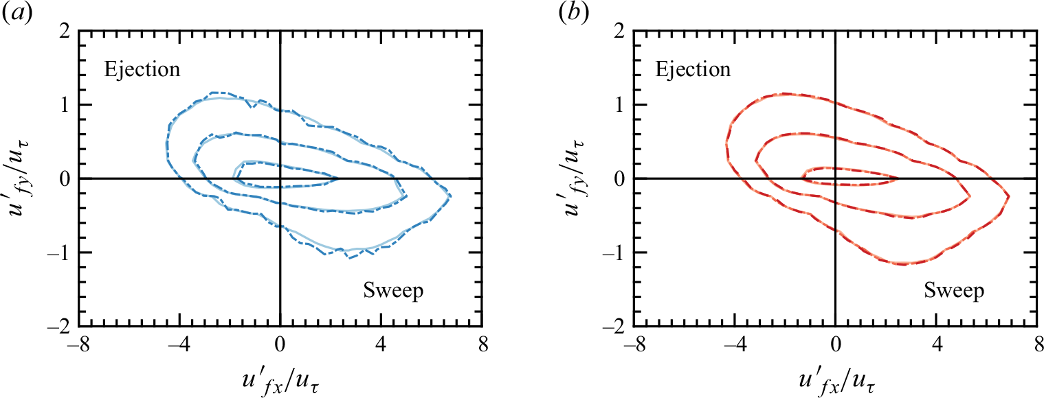
Figure 12 shows the joint probability density functions (PDF) of the particle-sampled fluid velocity fluctuations at
 $5 \leqslant y^+ \leqslant 30$
. For both
$5 \leqslant y^+ \leqslant 30$
. For both
 $St^+=32$
and
$St^+=32$
and
 $St^+=133$
, neutral particles show a tendency to sample Q2 and Q4 more frequently than Q1 and Q3. This confirms that ejections (Q2) and sweeps (Q4) play a dominant role in transporting particles near the wall. In figure 12(a), contours of the joint PDF of charged particles (
$St^+=133$
, neutral particles show a tendency to sample Q2 and Q4 more frequently than Q1 and Q3. This confirms that ejections (Q2) and sweeps (Q4) play a dominant role in transporting particles near the wall. In figure 12(a), contours of the joint PDF of charged particles (
 $St^+=32$
,
$St^+=32$
,
 $q=5 \times 10^{-15} \ \textrm{C}$
) are less smooth because of the lower particle concentration within the range
$q=5 \times 10^{-15} \ \textrm{C}$
) are less smooth because of the lower particle concentration within the range
 $5 \leqslant y^+ \leqslant 30$
(figure 6
a). Despite the reduced particle concentration, the general shape of the contours in the charged case remains similar to those of neutral particles. However, two differences are also observed: the portion of particles in Q2 decreases, while the portion of particles in Q4 increases. This trend is better highlighted by comparing the proportions of particles sampling Q2 and Q4, as summarised in table 4. As a result, charged particles sample less upward fluid velocities than neutral particles, which explains the consistent decrease of
$5 \leqslant y^+ \leqslant 30$
(figure 6
a). Despite the reduced particle concentration, the general shape of the contours in the charged case remains similar to those of neutral particles. However, two differences are also observed: the portion of particles in Q2 decreases, while the portion of particles in Q4 increases. This trend is better highlighted by comparing the proportions of particles sampling Q2 and Q4, as summarised in table 4. As a result, charged particles sample less upward fluid velocities than neutral particles, which explains the consistent decrease of
 $I_{bias}$
with the increase of
$I_{bias}$
with the increase of
 $q$
for
$q$
for
 $St^+=32$
in figure 10(a). The same trend is also observed for
$St^+=32$
in figure 10(a). The same trend is also observed for
 $St^+=133$
particles. However, since
$St^+=133$
particles. However, since
 $St^+=133$
particles are more inertial, the change in figure 12(b) is less significant, leading to a smaller change in
$St^+=133$
particles are more inertial, the change in figure 12(b) is less significant, leading to a smaller change in
 $I_{bias}$
(figure 10
b).
$I_{bias}$
(figure 10
b).
Proportion of particles sampling Q2 and Q4 within the range
 $5 \leqslant y^+ \leqslant 30$
.
$5 \leqslant y^+ \leqslant 30$
.
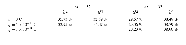
It is noteworthy that the observed trend of sampling less upward flows is similar to the phenomenon of preferential sweeping in the gravitational settling of heavy particles in turbulence. It is known that heavy particles settling in HIT may tend to sample the downward-velocity region of vortices, aligning with the direction of gravity. This behaviour leads to an enhanced average settling velocity of inertial particles (Wang & Maxey Reference Wang and Maxey1993; Bec et al. Reference Bec, Homann and Ray2014). Similarly, in wall-bounded turbulence, an analogous enhancement in settling velocity has been reported. Particles subject to a constant force directed towards the wall preferentially sample flow regions that are also moving towards the wall as they pass through the buffer layer, which effectively increases particles’ settling velocity (Chen et al. Reference Chen, Chen, Wu, Ruan and Li2022). Given that fluid sweeps are typically more intense and spatially concentrated than ejections, the bias introduced by the electrostatic force is even stronger compared with that in HIT. In the current study, the electrostatic force acting on charged particles plays a similar role to gravity in these previous studies. The particles are driven towards the wall by the electrostatic attraction, leading them to preferentially sample fluid motions that also move towards the wall. This leads to a reduction in upward-flow sampling (ejections) and an increase in downward-flow sampling (sweeps), thereby making a secondary contribution to the accumulation of particles near the wall. Furthermore, the electrostatic force is not uniform across the entire channel but becomes stronger closer to the wall, making its influence on biased sampling an increasingly important factor to consider.
In addition, in HIT, the gravitational settling velocity of heavy particles can be either enhanced or reduced, depending on the ratio of gravitational settling velocity to turbulence intensity. Accordingly, we expect to observe different regimes based on the relative importance of the wall-pointing electrostatic force compared with turbulent fluctuations. In this study, due to the low particle charge and concentration, the particle-induced electric field remains weak. As a result, the wall-pointing electrical migration velocity is small relative to turbulent fluctuations, which lies within the regime of preferential sweeping that leads to enhanced deposition. However, if the electrical migration velocity becomes more significant, such as in the presence of a strong external field or with highly charged particles, this enhancement may change. For instance, when the electrical migration velocity greatly exceeds turbulent fluctuations, particle behaviour may decouple from near-wall coherent structures, and the deposition enhancement is suppressed. However, when the electrical migration velocity becomes comparable to turbulent fluctuations, it remains unclear whether particles will experience a slowdown due to the loitering effect, as reported in previous works in HIT. This presents an interesting topic for future investigations.
3.4. Wall-normal electric field
In this section, we discuss the profile of the wall-normal electric field
 $E_y$
, which directly affects particle concentration through
$E_y$
, which directly affects particle concentration through
 $I_{elec}$
. Moreover,
$I_{elec}$
. Moreover,
 $E_y$
also serves as a direct indicator of the significance of the electrostatic force on particle behaviour.
$E_y$
also serves as a direct indicator of the significance of the electrostatic force on particle behaviour.
As suggested in Guha (Reference Guha2008), a particle
 $i$
with charge
$i$
with charge
 $q_i$
near a grounded conducting wall experiences the electrostatic force due to the induced charge on the wall, which equals the Coulomb force from its image located at the symmetric location about the wall with the opposite charge
$q_i$
near a grounded conducting wall experiences the electrostatic force due to the induced charge on the wall, which equals the Coulomb force from its image located at the symmetric location about the wall with the opposite charge
 $-q_i$
. If the PW distance is
$-q_i$
. If the PW distance is
 $y_w$
, the wall-normal electric field due to the PW interaction can be computed by
$y_w$
, the wall-normal electric field due to the PW interaction can be computed by
 \begin{equation} E_y^{(Im)}=-\frac {q_i}{4 \pi \varepsilon _0 (2 y_{w,i} )^2}=-\frac {q_i}{16 \pi \varepsilon _0 y_{w,i}^2}. \end{equation}
Averaged wall-normal electric field
 $\langle E_y \rangle$
for particles with (a)
$\langle E_y \rangle$
for particles with (a)
 $St^{+}=32$
and (b)
$St^{+}=32$
and (b)
 $St^{+}=133$
. Scatters with light to dark grey correspond to a particle charge of
$St^{+}=133$
. Scatters with light to dark grey correspond to a particle charge of
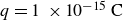 $q=1 \ \times 10^{-15} \ \textrm{C}$
, and
$q=1 \ \times 10^{-15} \ \textrm{C}$
, and
 $2 \ \times 10^{-15} \ \textrm{C}$
. Contributions from the PW and PP electrostatic interactions are shown as blue dashed lines and red dash-dotted lines, respectively.
$2 \ \times 10^{-15} \ \textrm{C}$
. Contributions from the PW and PP electrostatic interactions are shown as blue dashed lines and red dash-dotted lines, respectively.
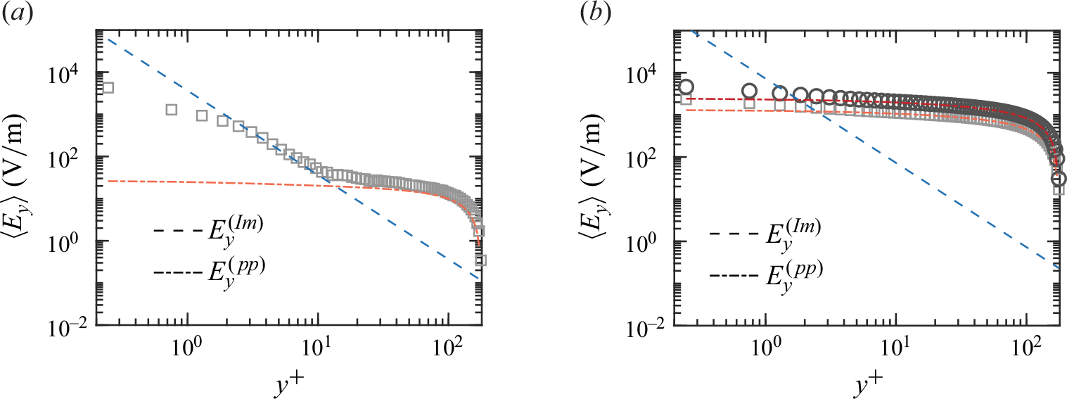
The average wall-normal electric field
 $\langle E_y \rangle$
for particles with
$\langle E_y \rangle$
for particles with
 $St^+=32$
and
$St^+=32$
and
 $q=5 \times 10^{-15} \ \textrm{C}$
is then compared with
$q=5 \times 10^{-15} \ \textrm{C}$
is then compared with
 $E_y^{(Im)}$
in figure 13(a). One notices that
$E_y^{(Im)}$
in figure 13(a). One notices that
 $E_y^{(Im)}$
collapses with the simulation results only within the intermediate range of
$E_y^{(Im)}$
collapses with the simulation results only within the intermediate range of
 $ 2 \leqslant y^+ \leqslant 10$
, while significant deviations occur in both the near-wall and far-field regions. These deviations indicate that the PW interaction alone cannot account for all the electrostatic forces acting on particles, highlighting the need to include the electric field generated by the PP electrostatic interaction. Thus, we derive the electric field due to the PP interaction,
$ 2 \leqslant y^+ \leqslant 10$
, while significant deviations occur in both the near-wall and far-field regions. These deviations indicate that the PW interaction alone cannot account for all the electrostatic forces acting on particles, highlighting the need to include the electric field generated by the PP electrostatic interaction. Thus, we derive the electric field due to the PP interaction,
 $\mathbf{E}^{(pp)}$
, starting from Gauss law
$\mathbf{E}^{(pp)}$
, starting from Gauss law
 \begin{equation} \boldsymbol{\nabla} \cdot \mathbf{E}^{(pp)}=\frac {\rho _c}{\varepsilon _0} = \frac {qC}{\varepsilon _0}. \end{equation}
Here, the volumetric charging density
 $\rho _c$
equals the product of the particle charge
$\rho _c$
equals the product of the particle charge
 $q$
and the particle concentration
$q$
and the particle concentration
 $C$
. Taking the ensemble average of (3.8) leads to
$C$
. Taking the ensemble average of (3.8) leads to
 \begin{equation} \frac {\textrm{d} \langle E_y^{(pp)} \rangle }{\textrm{d} y}=\frac {q\langle C \rangle }{\varepsilon _0}. \end{equation}
Note that in (3.9) the electric field components in periodic directions become zero after ensemble averaging, i.e.
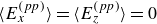 $\langle E_x^{(pp)} \rangle =\langle E_z^{(pp)} \rangle =0$
. Integrating (3.9) from a certain location
$\langle E_x^{(pp)} \rangle =\langle E_z^{(pp)} \rangle =0$
. Integrating (3.9) from a certain location
 $y$
to the centreline
$y$
to the centreline
 $\delta$
then yields
$\delta$
then yields
 \begin{align} \langle E_y^{(pp)} \rangle (\delta )-\langle E_y^{(pp)} \rangle (y)=\frac {q}{\varepsilon _0}\int _{\eta =y}^{\eta =\delta } \langle C \rangle (\eta ) \textrm{d}\eta . \end{align}
Considering the symmetry of the system, the wall-normal electric field at the centreline is zero, i.e.
 $\langle E_y^{(pp)} \rangle (\delta )=0$
. Therefore, the PP electric field is
$\langle E_y^{(pp)} \rangle (\delta )=0$
. Therefore, the PP electric field is
 \begin{equation} \langle E_y^{(pp)} \rangle (y)=-\frac {q}{\varepsilon _0}\int _{\eta =y}^{\eta =\delta } \langle C \rangle (\eta ) \textrm{d}\eta . \end{equation}
In (3.11),
 $\langle E_y^{(pp)} \rangle (y)$
is negative, indicating the PP electrostatic force always points towards the wall. Specifically, for a target particle located at
$\langle E_y^{(pp)} \rangle (y)$
is negative, indicating the PP electrostatic force always points towards the wall. Specifically, for a target particle located at
 $y$
, the net PP electrostatic force equals the Coulomb repulsion from all the particles located between
$y$
, the net PP electrostatic force equals the Coulomb repulsion from all the particles located between
 $y$
to the centreline
$y$
to the centreline
 $\delta$
, which pushes the target particle towards the wall. The PP electric field
$\delta$
, which pushes the target particle towards the wall. The PP electric field
 $\langle E_y^{(pp)} \rangle (y)$
is then plotted in figure 13(a) as a red dash-dotted line, which agrees with the simulation results in the far-field region (
$\langle E_y^{(pp)} \rangle (y)$
is then plotted in figure 13(a) as a red dash-dotted line, which agrees with the simulation results in the far-field region (
 $y^+ \geqslant 20$
).
$y^+ \geqslant 20$
).
We therefore propose three distinct regions of the wall-normal electric field, as illustrated in figure 13(a). In the far-field region at large
 $y^+$
, the contribution from the PW interaction is negligible compared with the PP interaction. Particles in this region are primarily driven towards the wall by PP Coulomb repulsion. As
$y^+$
, the contribution from the PW interaction is negligible compared with the PP interaction. Particles in this region are primarily driven towards the wall by PP Coulomb repulsion. As
 $y^+$
decreases,
$y^+$
decreases,
 $\langle E_y^{(Im)} \rangle (y)$
levels off as the integral in (3.11) saturates, while the PW interaction continues to rise and eventually becomes dominant. Consequently, the PW interaction prevails as the primary electrostatic force in the intermediate region. Finally, when the particle approaches the wall, the repulsion from the concentrated particles counteracts the PW attraction, resulting in
$\langle E_y^{(Im)} \rangle (y)$
levels off as the integral in (3.11) saturates, while the PW interaction continues to rise and eventually becomes dominant. Consequently, the PW interaction prevails as the primary electrostatic force in the intermediate region. Finally, when the particle approaches the wall, the repulsion from the concentrated particles counteracts the PW attraction, resulting in
 $\langle E_y \rangle (y)$
being lower than that predicted by (3.7).
$\langle E_y \rangle (y)$
being lower than that predicted by (3.7).
Interestingly, not all three regions exist in all cases, as shown in figure 13(b) for charged particles with
 $St^+=133$
. The transition between the intermediate and the far-field regions depends on the relative importance of the PW and the PP interactions
$St^+=133$
. The transition between the intermediate and the far-field regions depends on the relative importance of the PW and the PP interactions
 \begin{equation} \underbrace {\frac {q}{16 \pi \varepsilon _0 y_{w}^2}}_{\text{PW interaction}}, \ \text{and} \ \underbrace {\frac {1}{\varepsilon _0}\int _{\eta =y}^{\eta =\delta } [q \times \langle C \rangle (\eta )] \textrm{d}\eta }_{\text{PP interaction}}. \end{equation}
As shown in figure 6(b), the particle concentration
 $C(y)$
for
$C(y)$
for
 $St^+=133$
is high in the outer flow, leading to a more pronounced PP interaction. Consequently, the PP interaction dominates nearly up to the wall. In such cases, relying solely on the image charge force would significantly underestimate the magnitude of the electrostatic force.
$St^+=133$
is high in the outer flow, leading to a more pronounced PP interaction. Consequently, the PP interaction dominates nearly up to the wall. In such cases, relying solely on the image charge force would significantly underestimate the magnitude of the electrostatic force.
In the end, discussing the relative importance of the PW and the PP electrostatic interactions across a broader range of scenarios is essential for developing a more complete understanding of the electrostatic effects arising from particle charging. In this study, the particles are monodispersed and identically charged, meaning that the net charge between
 $y$
and
$y$
and
 $\delta$
in (3.11) is always non-zero, resulting in a net repulsive force. The significance of this repulsion depends on the net charge distribution within the channel. With a much lower particle concentration, the PP interaction is expected to be less influential, allowing the PW interaction to dominate at larger
$\delta$
in (3.11) is always non-zero, resulting in a net repulsive force. The significance of this repulsion depends on the net charge distribution within the channel. With a much lower particle concentration, the PP interaction is expected to be less influential, allowing the PW interaction to dominate at larger
 $y^+$
. In addition, for monodispersed particles carrying both positive and negative charges, as is common in triboelectrification, the PP interaction becomes negligible because the integral of the net charge in (3.11) equals zero. However, in more complex systems with bidispersed oppositely charged particles, the concentration profiles for different particle groups will differ. Even if the overall system is neutral, there will be a separation between the centres of positive and negative centres. Consequently, the PP interaction will migrate light particles accumulated near the wall outward, while attracting heavy particles dispersed in the outer layer towards the wall, as reported by Zhang et al. (Reference Zhang, Cui and Zheng2023a
). Finally, beyond the channel flow investigated here, the transport of charged particles in turbulent boundary layers, such as sandstorms and pollutants dispersion in the atmosphere, is also widespread. In these systems, where there is only one wall, the PP interaction can still be evaluated by adjusting the upper limit
$y^+$
. In addition, for monodispersed particles carrying both positive and negative charges, as is common in triboelectrification, the PP interaction becomes negligible because the integral of the net charge in (3.11) equals zero. However, in more complex systems with bidispersed oppositely charged particles, the concentration profiles for different particle groups will differ. Even if the overall system is neutral, there will be a separation between the centres of positive and negative centres. Consequently, the PP interaction will migrate light particles accumulated near the wall outward, while attracting heavy particles dispersed in the outer layer towards the wall, as reported by Zhang et al. (Reference Zhang, Cui and Zheng2023a
). Finally, beyond the channel flow investigated here, the transport of charged particles in turbulent boundary layers, such as sandstorms and pollutants dispersion in the atmosphere, is also widespread. In these systems, where there is only one wall, the PP interaction can still be evaluated by adjusting the upper limit
 \begin{align} \langle E_y^{(pp)} \rangle (y)=\langle E_y^{(pp)} \rangle (y_{Ref})-\frac {1}{\varepsilon _0}\int _{\eta =y}^{\eta =y_{Ref}} q\langle C \rangle (\eta ) \textrm{d}\eta . \end{align}
Here,
 $\langle E_y^{(pp)} \rangle (y_{Ref})$
is the electric field at a reference point
$\langle E_y^{(pp)} \rangle (y_{Ref})$
is the electric field at a reference point
 $y_{Ref}$
. Thus, the PP interaction may still play a role as long as the net charge integral is significant.
$y_{Ref}$
. Thus, the PP interaction may still play a role as long as the net charge integral is significant.
4. Conclusions
This work utilises four-way coupled simulations to address an important question: How does particle charging affect the deposition velocity of particles onto an electrically grounded conductor through a turbulence boundary layer, particularly in the context of charged particle deposition in gas turbines? In this study, we developed a canonical case involving charged particles transported in a fully developed turbulent channel flow. Contrary to previous model predictions, which suggested no change in deposition velocity when particles are inertial and dominated by the turbophoresis effect, we found that electrostatic forces actually increase the deposition velocity.
Since the increase in the deposition velocity of charged particles primarily results from the enhanced near-wall accumulation, the wall-normal profile of charged particles is further examined. By employing a statistical approach in the particle phase space
 $(y,v_{py})$
, three mechanisms affecting the concentration profiles can be quantified in the form of integrals: turbophoresis (
$(y,v_{py})$
, three mechanisms affecting the concentration profiles can be quantified in the form of integrals: turbophoresis (
 $I_{turb}$
), biased sampling (
$I_{turb}$
), biased sampling (
 $I_{bias}$
) and electrostatic forces (
$I_{bias}$
) and electrostatic forces (
 $I_{elec}$
). It was found that the electrostatic force creates a sharper gradient in the wall-normal particle r.m.s. velocity, which significantly increases
$I_{elec}$
). It was found that the electrostatic force creates a sharper gradient in the wall-normal particle r.m.s. velocity, which significantly increases
 $I_{turb}$
. As a result, the enhanced turbophoresis effect is identified as the main driver of the more extreme particle accumulation near the wall. In addition, charged particles are found to sample upward-flow regions less frequently than neutral particles, which reduces the biased-sampling effect
$I_{turb}$
. As a result, the enhanced turbophoresis effect is identified as the main driver of the more extreme particle accumulation near the wall. In addition, charged particles are found to sample upward-flow regions less frequently than neutral particles, which reduces the biased-sampling effect
 $I_{bias}$
. This change occurs because charged particles subject to the wall-pointing electrostatic force tend to sample the downward-moving fluids as they pass through coherent structures in the buffer layer. This behaviour is analogous to the preferential sweeping effect observed in the settling of heavy particles in turbulence. Finally, the profile of the wall-normal electric field is discussed. It is found that both the PW interaction and the PP interaction contribute to the electrostatic force acting on charged particles. Depending on the conditions, the relative importance of the PW and PP interactions results in distinct electric field profiles. Consequently, when the net charge carried by suspended particles is significant, relying solely on the classic image charge model may lead to a significant underestimation of the electrostatic effects.
$I_{bias}$
. This change occurs because charged particles subject to the wall-pointing electrostatic force tend to sample the downward-moving fluids as they pass through coherent structures in the buffer layer. This behaviour is analogous to the preferential sweeping effect observed in the settling of heavy particles in turbulence. Finally, the profile of the wall-normal electric field is discussed. It is found that both the PW interaction and the PP interaction contribute to the electrostatic force acting on charged particles. Depending on the conditions, the relative importance of the PW and PP interactions results in distinct electric field profiles. Consequently, when the net charge carried by suspended particles is significant, relying solely on the classic image charge model may lead to a significant underestimation of the electrostatic effects.
According to the original framework of Guha (Reference Guha2008), the deposition velocity incorporates contributions from both the wall-normal particle concentration and velocity. To predict the deposition velocity for charged particles, it is assumed (i) that the particle velocity is modulated solely by the image force, and (ii) that the particle concentration remains unchanged. Upon carefully analysing our simulation results, these assumptions are found to be invalid. First, the wall-normal electrostatic force comprises contributions from both PP and PW interactions, whereas the classic model only accounts for the latter. In certain cases, such as figure 13(b), this omission leads to a significant underestimation of the magnitude of the electrostatic force. Second, as shown in figure 6, electrostatic forces drastically modulate particle concentration, which is the primary contributor to the increased deposition in this study. This critical effect is entirely absent in the classic model. Given that the one-dimensional Eulerian model has been widely used across various communities, it is crucial to highlight these limitations to ensure proper interpretation and application.
Regarding the physical process itself, several findings about its highly coupled nature are also presented. First, and most counterintuitively, the influence of electrostatic force is affected by particle–turbulence interaction. Since the PP electrostatic force depends on the concentration profile (3.11), the spatial distribution of particles determines the dominant electrostatic force, as illustrated by the distinct electric field profiles shown in figure 13. Consequently, a careful comparison of the relative importance of PP and PW electrostatic interactions is necessary. In contrast, many earlier studies often assumed the dominance of the image force without question. Second, turbophoresis, the primary mechanism that shapes the particle profile (figure 10), is found to be highly sensitive to the wall-normal r.m.s. velocity of the particles (
 $v_{p,rms}^+$
). Even a subtle change in
$v_{p,rms}^+$
). Even a subtle change in
 $v_{p,rms}^+$
(figure 11) can lead to a drastic change in the particle concentration profile. Therefore, in future studies, any factor that might affect
$v_{p,rms}^+$
(figure 11) can lead to a drastic change in the particle concentration profile. Therefore, in future studies, any factor that might affect
 $v_{p,rms}^+$
should be treated carefully, such as electrostatic forces, two-way coupling, and PP collisions. Moreover, although the current system is dilute, the effects of two-way coupling and interparticle collisions should still be accounted for, as the non-uniform particle concentration may locally transition into the two-way or four-way coupled regime.
$v_{p,rms}^+$
should be treated carefully, such as electrostatic forces, two-way coupling, and PP collisions. Moreover, although the current system is dilute, the effects of two-way coupling and interparticle collisions should still be accounted for, as the non-uniform particle concentration may locally transition into the two-way or four-way coupled regime.
Finally, it would also be valuable to discuss the potential influences of various parameters, such as the turbulence Reynolds number and particle inertia, on the findings of this study. The motivation for this work is to investigate the dust ingestion problem in jet engines. Due to the small characteristic length scales of the internal flow and the higher fluid viscosity at elevated operating temperatures Lawson & Thole (Reference Lawson and Thole2011), the friction Reynolds number is not expected to be extremely high. For example, the diameter of the cooling hole is given as
 $1.69\times 10^{-3} \ \textrm{m}$
in Lawson & Thole (Reference Lawson and Thole2011) and
$1.69\times 10^{-3} \ \textrm{m}$
in Lawson & Thole (Reference Lawson and Thole2011) and
 $4.6\times 10^{-3} \ \textrm{m}$
in Lawson & Thole (Reference Lawson and Thole2010). By choosing the radius of the hole as the half-channel width
$4.6\times 10^{-3} \ \textrm{m}$
in Lawson & Thole (Reference Lawson and Thole2010). By choosing the radius of the hole as the half-channel width
 $\delta$
, and considering the friction velocity
$\delta$
, and considering the friction velocity
 $u_{\tau }=3.59 \ {\textrm{m s}^{-1}}$
, the fluid density
$u_{\tau }=3.59 \ {\textrm{m s}^{-1}}$
, the fluid density
 $\rho _f=3.32 \ {\textrm{kg m}^{-3}}$
and the fluid viscosity
$\rho _f=3.32 \ {\textrm{kg m}^{-3}}$
and the fluid viscosity
 $\mu _f=5.55 \times 10^{-5} \ \textrm{Pa} \cdot \textrm{s}$
in § 2.1, the friction Reynolds number lies within the range of 180 to 490. Thus, the chosen
$\mu _f=5.55 \times 10^{-5} \ \textrm{Pa} \cdot \textrm{s}$
in § 2.1, the friction Reynolds number lies within the range of 180 to 490. Thus, the chosen
 $Re_{\tau }$
is within the parameter space for internal deposition. For external deposition, the Reynolds number may be even higher because of the high speed and large length scales. However, the key physics that drives particle deposition, i.e. particle inertia and electrostatics, will remain valid. Therefore, we choose
$Re_{\tau }$
is within the parameter space for internal deposition. For external deposition, the Reynolds number may be even higher because of the high speed and large length scales. However, the key physics that drives particle deposition, i.e. particle inertia and electrostatics, will remain valid. Therefore, we choose
 $Re_{\tau } = 180$
to keep the flow configurations similar to those in our experimental investigations on the transport and deposition of charged inertial particles in a vertical turbulent channel, where
$Re_{\tau } = 180$
to keep the flow configurations similar to those in our experimental investigations on the transport and deposition of charged inertial particles in a vertical turbulent channel, where
 $Re_{\tau } \approx 200$
. As discussed by Johnson et al. (Reference Johnson, Bassenne and Moin2020), the transport mechanisms (turbophoresis and biased sampling) of neutral particles appear consistent across multiple Reynolds numbers. Consequently, the modulation of particle deposition velocity by electrostatic forces is also expected to remain consistent, allowing the findings of this study to be extended to high Reynolds numbers that are more representative of realistic flow conditions.
$Re_{\tau } \approx 200$
. As discussed by Johnson et al. (Reference Johnson, Bassenne and Moin2020), the transport mechanisms (turbophoresis and biased sampling) of neutral particles appear consistent across multiple Reynolds numbers. Consequently, the modulation of particle deposition velocity by electrostatic forces is also expected to remain consistent, allowing the findings of this study to be extended to high Reynolds numbers that are more representative of realistic flow conditions.
Although inertial particles are discussed in this study, how electrostatic force affects the deposition of tracer-like particles is also relevant in many applications. For inertialess particles, the contributions of turbophoresis and biased sampling are no longer present, meaning that the enhancement of particle deposition arises only from the direct effect of
 $I_{elec}$
. In this case, the wall-normal electrostatic force becomes the primary mechanism that enhances deposition, which depends on the particle charging conditions. In a system where tracer particles carry both positive and negative charges, the PP electrostatic force (
$I_{elec}$
. In this case, the wall-normal electrostatic force becomes the primary mechanism that enhances deposition, which depends on the particle charging conditions. In a system where tracer particles carry both positive and negative charges, the PP electrostatic force (
 $E_y^{(pp)}$
) is zero, and the dominant force is the image force (
$E_y^{(pp)}$
) is zero, and the dominant force is the image force (
 $E_y^{(Im)}$
) due to the PW electrostatic force. According to Yao & Capecelatro (Reference Yao and Capecelatro2021), under these conditions, tracers follow local fluid motions faithfully when away from the wall, but detach from the local flow and accelerate towards the wall as they approach the near-wall region, where the image force becomes significant. As a result, the influence of PW interaction is limited to the near-wall region. If tracers are identically charged, in addition to the image forces, the PP electrostatic repulsion (
$E_y^{(Im)}$
) due to the PW electrostatic force. According to Yao & Capecelatro (Reference Yao and Capecelatro2021), under these conditions, tracers follow local fluid motions faithfully when away from the wall, but detach from the local flow and accelerate towards the wall as they approach the near-wall region, where the image force becomes significant. As a result, the influence of PW interaction is limited to the near-wall region. If tracers are identically charged, in addition to the image forces, the PP electrostatic repulsion (
 $E_y^{(pp)}$
) contributes significantly to the far field (figure 13). Consequently, tracer trajectories may detach from local streamlines even when they are still far from the wall. Meanwhile, as the electrostatic force grows increasingly significant near the wall, the particle slip velocity will show a continuous increase as particles approach the wall. In addition to the driving mechanism, the resistance to tracer deposition is also of interest. For inertial particles, biased sampling serves as the primary mechanism that pushes particles away from the wall. However, this mechanism is absent for tracers. Consequently, the resistance to tracer deposition is also expected to arise from the electrostatic force. For identically charged tracers, as particles accumulate near the wall, the mutual repulsion between them also grows. If the wall is not grounded or is made of dielectric material, the local electric potential continues to rise, which effectively repels new incoming particles. As a result, a balance is established between the wall-approaching attraction and the near-wall repulsion, leading to a steady state. However, if (i) the particles carry opposite charges, eliminating mutual repulsion, or (ii) the wall is conducting and grounded, causing the mutual repulsion to be largely suppressed by the image force effect, the electric potential near the wall will remain close to zero. Consequently, there is no resisting force to prevent particle deposition. In this case, a steady state cannot be achieved, and all particles will eventually migrate towards the wall and become captured.
$E_y^{(pp)}$
) contributes significantly to the far field (figure 13). Consequently, tracer trajectories may detach from local streamlines even when they are still far from the wall. Meanwhile, as the electrostatic force grows increasingly significant near the wall, the particle slip velocity will show a continuous increase as particles approach the wall. In addition to the driving mechanism, the resistance to tracer deposition is also of interest. For inertial particles, biased sampling serves as the primary mechanism that pushes particles away from the wall. However, this mechanism is absent for tracers. Consequently, the resistance to tracer deposition is also expected to arise from the electrostatic force. For identically charged tracers, as particles accumulate near the wall, the mutual repulsion between them also grows. If the wall is not grounded or is made of dielectric material, the local electric potential continues to rise, which effectively repels new incoming particles. As a result, a balance is established between the wall-approaching attraction and the near-wall repulsion, leading to a steady state. However, if (i) the particles carry opposite charges, eliminating mutual repulsion, or (ii) the wall is conducting and grounded, causing the mutual repulsion to be largely suppressed by the image force effect, the electric potential near the wall will remain close to zero. Consequently, there is no resisting force to prevent particle deposition. In this case, a steady state cannot be achieved, and all particles will eventually migrate towards the wall and become captured.
Funding.
This work was supported by the Office of Naval Research (ONR) under Grant NO. N00014-21-1-2620. This work was also partially supported by an Early Stage Innovation grant from NASA’s Space Technology Research Grants Program under Grant NO. 80NSSC21K0222.
Declaration of interests.
The authors report no conflict of interest.
Appendix A. Assessment of grid resolution
In the main text, a Cartesian grid with a resolution of
 $128^3$
is used. The grid is uniform in both the
$128^3$
is used. The grid is uniform in both the
 $x$
and
$x$
and
 $z$
directions, and stretched in the
$z$
directions, and stretched in the
 $y$
direction with a stretching factor of
$y$
direction with a stretching factor of
 $S=1.9$
. To assess grid sensitivity, we simulated test cases on a refined grid with a resolution of
$S=1.9$
. To assess grid sensitivity, we simulated test cases on a refined grid with a resolution of
 $256^3$
and the same stretching factor. The grid information is summarised in table 5.
$256^3$
and the same stretching factor. The grid information is summarised in table 5.
Summary of grid assessment.
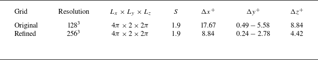
Two different Stokes numbers (
 $St^+=32/133$
) are used in the tests while the particle charge is set to zero. The fluid velocity profiles for the two grid resolutions are shown in figure 14, while particle concentration and velocity profiles are compared in figure 15. Most fluid and particle statistics remain unchanged when the mesh is refined. The wall-normal particle r.m.s. velocity (figure 15
c) shows a slight increase near the channel centre on the refined mesh. However, this does not lead to any significant modulation in particle concentration, as observed in figure 15(a). Therefore, the grid resolution of
$St^+=32/133$
) are used in the tests while the particle charge is set to zero. The fluid velocity profiles for the two grid resolutions are shown in figure 14, while particle concentration and velocity profiles are compared in figure 15. Most fluid and particle statistics remain unchanged when the mesh is refined. The wall-normal particle r.m.s. velocity (figure 15
c) shows a slight increase near the channel centre on the refined mesh. However, this does not lead to any significant modulation in particle concentration, as observed in figure 15(a). Therefore, the grid resolution of
 $128^3$
used in the main text is deemed sufficient.
$128^3$
used in the main text is deemed sufficient.
Mean streamwise fluid velocity in the case with (a)
 $St^+=32$
and (c)
$St^+=32$
and (c)
 $St^+=133$
. Root mean square of fluid fluctuation velocity in
$St^+=133$
. Root mean square of fluid fluctuation velocity in
 $x$
,
$x$
,
 $y$
,
$y$
,
 $z$
directions for (b)
$z$
directions for (b)
 $St^+=32$
and (d)
$St^+=32$
and (d)
 $St^+=133$
. Crosses (
$St^+=133$
. Crosses (
 $x$
) represent results using the original grid mesh (
$x$
) represent results using the original grid mesh (
 $128^3$
), and circles (
$128^3$
), and circles (
 $\circ$
) denote results using a refined mesh (
$\circ$
) denote results using a refined mesh (
 $256^3$
).
$256^3$
).
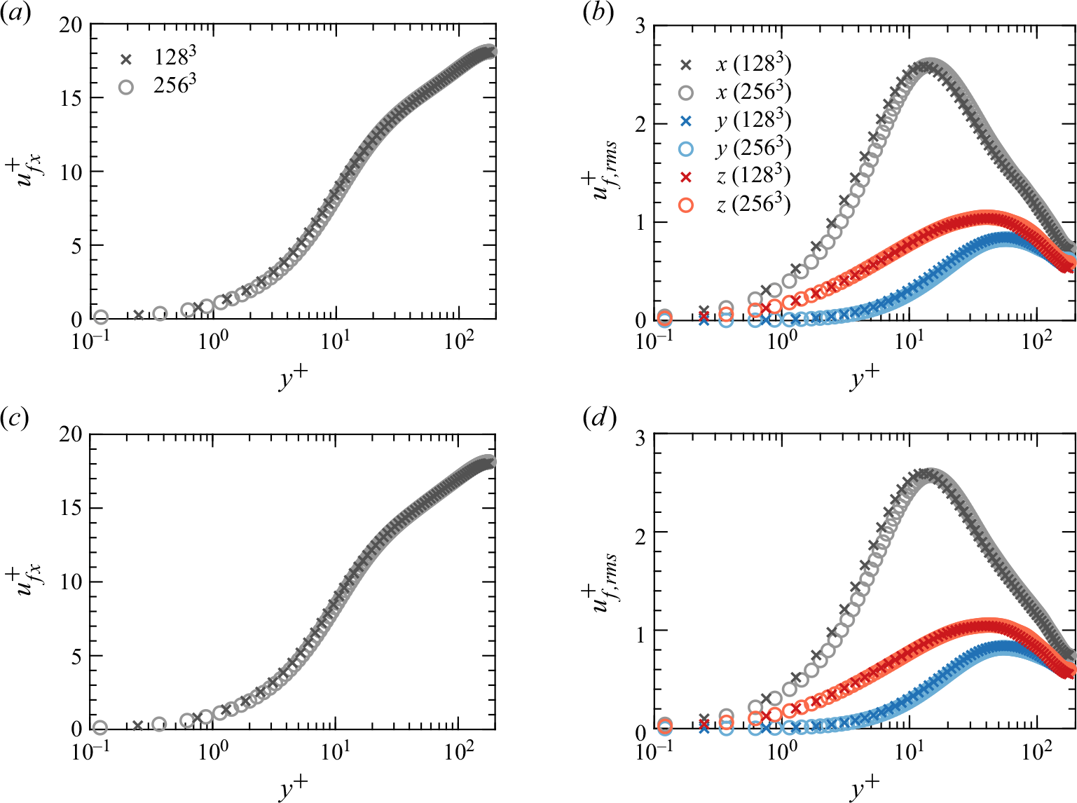
Comparison of (a) normalised wall-normal particle concentration
 $C/C_0$
, (b) mean streamwise particle velocity and (c) r.m.s. of wall-normal particle fluctuation velocity. Crosses (
$C/C_0$
, (b) mean streamwise particle velocity and (c) r.m.s. of wall-normal particle fluctuation velocity. Crosses (
 $x$
) represent results using the original grid mesh (
$x$
) represent results using the original grid mesh (
 $128^3$
), and circles (
$128^3$
), and circles (
 $\circ$
) denote results using a refined mesh (
$\circ$
) denote results using a refined mesh (
 $256^3$
).
$256^3$
).
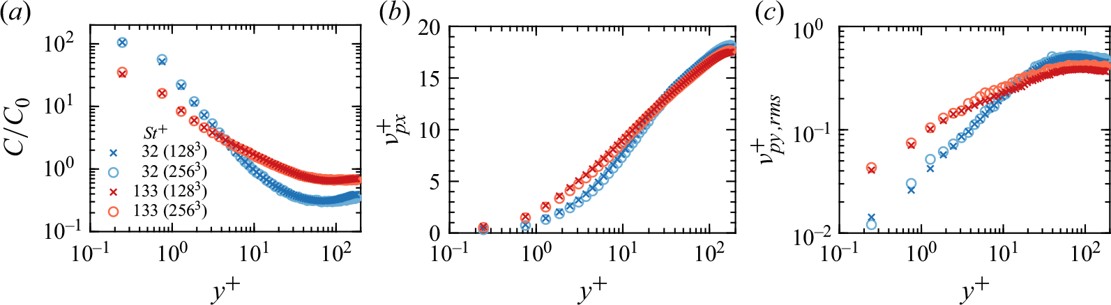
Appendix B. Volume-filtered Eulerian–Lagrangian framework
This section presents a brief derivation of the governing equations of the volume-filtered Eulerian–Lagrangian (VFEL) framework employed in this work. During the derivation, certain simplifications are made to obtain the final form presented in the main text. Justifications for these simplifications are also provided below. Further details about the VFEL framework can be found in Capecelatro & Desjardins (Reference Capecelatro and Desjardins2013)and Anderson & Jackson (Reference Anderson and Jackson1967).
B.1 Governing equations of fluid motion
In the standard point-wise Eulerian–Lagrangian approach, the governing equations of the fluid phase without body forces are
 \begin{equation} \frac {\partial {\rho _f}}{\partial t} + \boldsymbol{\nabla} \cdot (\rho _f \mathbf{u}_f) = 0, \end{equation}
 \begin{equation} \frac {\partial (\rho _f \mathbf{u}_f)}{\partial t} + \boldsymbol{\nabla} \cdot (\rho _f \mathbf{u}_f \otimes \mathbf{u}_f) = \boldsymbol{\nabla} \cdot \boldsymbol{\tau }. \end{equation}
Here,
 $\rho _f$
and
$\rho _f$
and
 $\mathbf{u}_f$
are the density and velocity of the fluid. The fluid stress is given by
$\mathbf{u}_f$
are the density and velocity of the fluid. The fluid stress is given by
 \begin{equation} \boldsymbol{\tau }=-p \mathbf{I} + \mu _f \left [ (\boldsymbol{\nabla} \mathbf{u}_f+{\boldsymbol{\nabla} \mathbf{u}_f}^T) - \cfrac {2}{3}(\boldsymbol{\nabla} \cdot \mathbf{u}_f)\mathbf{I} \right ], \end{equation}
where
 $p$
and
$p$
and
 $\mu _f$
are the fluid pressure and dynamic viscosity. A Gaussian filter
$\mu _f$
are the fluid pressure and dynamic viscosity. A Gaussian filter
 $G_F$
is then defined as
$G_F$
is then defined as
 \begin{align} G_F(r)=\frac {1}{\sqrt {2 \pi }\sigma } \exp {\left ( -\frac {r^2}{2 \sigma ^2} \right )}. \end{align}
The filter length
 $\delta _F$
, defined as the width of
$\delta _F$
, defined as the width of
 $G_F(r)$
at the half-height, can be related to
$G_F(r)$
at the half-height, can be related to
 $\sigma$
as
$\sigma$
as
 $\delta _F=2 \sqrt {2 \ln {2}} \sigma$
. The fluid volume fraction can then be defined as
$\delta _F=2 \sqrt {2 \ln {2}} \sigma$
. The fluid volume fraction can then be defined as
 \begin{equation} \alpha _f(\mathbf{x},t)=\int _{\mathcal{V}_f} G_F(|\mathbf{x}-\mathbf{y}|) \textrm{d} \mathbf{y}, \end{equation}
where
 $\mathcal{V}_f$
means the integral is taken over all points
$\mathcal{V}_f$
means the integral is taken over all points
 $\mathbf{y}$
occupied by the fluid phase. Applying the Gaussian filter to any point property
$\mathbf{y}$
occupied by the fluid phase. Applying the Gaussian filter to any point property
 $\mathbf{a}(\mathbf{x},t)$
of the fluid then yields
$\mathbf{a}(\mathbf{x},t)$
of the fluid then yields
 \begin{equation} \alpha _f \overline {\mathbf{a}}(\mathbf{x},t) = \int _{\mathcal{V}_f} \mathbf{a}(\mathbf{x},t) G_F(|\mathbf{x}-\mathbf{y}|) \textrm{d} \mathbf{y}, \end{equation}
where
 $\overline {\mathbf{a}}(\mathbf{x},t)$
is the volume-filtered property. The associated residual can be written as
$\overline {\mathbf{a}}(\mathbf{x},t)$
is the volume-filtered property. The associated residual can be written as
 $\mathbf{a}^{\prime } (\mathbf{x},t)=\mathbf{a}(\mathbf{x},t)-\overline {\mathbf{a}}(\mathbf{x},t)$
.
$\mathbf{a}^{\prime } (\mathbf{x},t)=\mathbf{a}(\mathbf{x},t)-\overline {\mathbf{a}}(\mathbf{x},t)$
.
We now derive the volume-filtered motion equations. By assuming that the shortest distance from
 $\mathbf{x}$
to the boundaries of the system is much larger than the filter size, Anderson & Jackson (Reference Anderson and Jackson1967) derived the volume filtering of the temporal derivative, divergence and gradient of a point property as
$\mathbf{x}$
to the boundaries of the system is much larger than the filter size, Anderson & Jackson (Reference Anderson and Jackson1967) derived the volume filtering of the temporal derivative, divergence and gradient of a point property as
 \begin{equation} \int _{\mathcal{V}_f} \frac {\partial \mathbf{a}(\mathbf{y},t)}{\partial t} G_F(|\mathbf{x}-\mathbf{y}|) \textrm{d} \mathbf{y}= \frac {\partial }{\partial t}(\alpha _f \overline {\mathbf{a}}(\mathbf{x},t))+\sum _{i=1}^{N_p}\int _{\mathcal{S}_i} \mathbf{n} \cdot \mathbf{u}_i \mathbf{a}(\mathbf{y},t)G_F(|\mathbf{x}-\mathbf{y}|)\textrm{d} \mathbf{y}, \end{equation}
 \begin{equation} \int _{\mathcal{V}_f} \boldsymbol{\nabla} \cdot \mathbf{a}(\mathbf{y},t) G_F(|\mathbf{x}-\mathbf{y}|) \textrm{d} \mathbf{y}=\boldsymbol{\nabla} \cdot (\alpha _f \overline {\mathbf{a}}(\mathbf{x},t))-\sum _{i=1}^{N_p}\int _{\mathcal{S}_i} \mathbf{n}\cdot \mathbf{a}(\mathbf{y},t)G_F(|\mathbf{x}-\mathbf{y}|)\textrm{d} \mathbf{y}, \end{equation}
 \begin{equation} \int _{\mathcal{V}_f} \boldsymbol{\nabla} \mathbf{a}(\mathbf{y},t) G_F(|\mathbf{x}-\mathbf{y}|) \textrm{d} \mathbf{y}=\boldsymbol{\nabla} (\alpha _f \overline {\mathbf{a}}(\mathbf{x},t))-\sum _{i=1}^{N_p}\int _{\mathcal{S}_i} \mathbf{n}\otimes \mathbf{a}(\mathbf{y},t)G_F(|\mathbf{x}-\mathbf{y}|)\textrm{d} \mathbf{y}. \end{equation}
Here,
 $\mathcal{S}_i$
represents the spherical surface of particle
$\mathcal{S}_i$
represents the spherical surface of particle
 $i$
,
$i$
,
 $\mathbf{n}$
is the outward unit vector on the particle surface and
$\mathbf{n}$
is the outward unit vector on the particle surface and
 $\mathbf{u}_i$
denotes the velocity of the solid matter at point
$\mathbf{u}_i$
denotes the velocity of the solid matter at point
 $\mathbf{y}$
on
$\mathbf{y}$
on
 $\mathcal{S}_i$
. Since there is no mass transfer between the solid and fluid phases,
$\mathcal{S}_i$
. Since there is no mass transfer between the solid and fluid phases,
 $\mathbf{u}_i$
is equal to the fluid velocity at the particle surface.
$\mathbf{u}_i$
is equal to the fluid velocity at the particle surface.
For a constant-density fluid, multiplying (B1a
) by
 $G_F$
and integrating over
$G_F$
and integrating over
 $\mathcal{V}_f$
, followed by the application of (B6a
) and (B6b
), yields the volume-filtered continuity equation
$\mathcal{V}_f$
, followed by the application of (B6a
) and (B6b
), yields the volume-filtered continuity equation
 \begin{equation} \frac {\partial \alpha _f}{\partial t} + \boldsymbol{\nabla} \cdot (\alpha _f \overline {\mathbf{u}}_f)=0. \end{equation}
Similarly, volume filtering the left-hand side of (B1b ) and again applying (B6a ) and (B6b ) results in
 \begin{equation} \frac {\partial }{\partial t}(\alpha _f \rho _f \overline {\mathbf{u}}_f) + \boldsymbol{\nabla} \cdot (\alpha _f \rho _f \overline {\mathbf{u}}_f \otimes \overline {\mathbf{u}}_f) + \boldsymbol{\nabla} \cdot (\alpha _f \rho _f \overline {\mathbf{u}_f^\prime \otimes \mathbf{u}_f^\prime }), \end{equation}
where the residual Reynolds stress is
 \begin{equation} \mathcal{F}_{u}=\boldsymbol{\nabla} \cdot (\alpha _f \rho _f \overline {\mathbf{u}_f^\prime \otimes \mathbf{u}_f^\prime }). \end{equation}
The volume filtering of the right-hand side of (B1b
) can be obtained by substituting
 $\mathbf{a}=\boldsymbol{\tau }$
in (B6b
), which reads
$\mathbf{a}=\boldsymbol{\tau }$
in (B6b
), which reads
 \begin{equation} \int _{\mathcal{V}_f} \boldsymbol{\nabla} \cdot \boldsymbol{\tau }(\mathbf{y},t) G_F(|\mathbf{x}-\mathbf{y}|) \textrm{d} \mathbf{y}=\boldsymbol{\nabla} \cdot (\alpha _f \overline {\boldsymbol{\tau }})-\sum _{i=1}^{N_p}\int _{\mathcal{S}_i} \mathbf{n}\cdot \boldsymbol{\tau }(\mathbf{y},t)G_F(|\mathbf{x}-\mathbf{y}|)\textrm{d} \mathbf{y}, \end{equation}
where the filtered stress is written as
 \begin{equation} \overline {\boldsymbol{\tau }}=\overline {\boldsymbol{\tau }}^* + \boldsymbol{\tau }_{\mu } = -\overline {p} \mathbf{I} + \mu _f \left [ (\boldsymbol{\nabla} \overline {\boldsymbol{\mathbf{u}}}_f+{\boldsymbol{\nabla} \overline {\mathbf{u}}_f}^T) - \cfrac {2}{3}(\boldsymbol{\nabla} \cdot \overline {\mathbf{u}}_f)\mathbf{I} \right ] + \boldsymbol{\tau }_{\mu }. \end{equation}
Here,
 $\overline {\boldsymbol{\tau }}^*$
is the nominal stress evaluated using the filtered velocity field
$\overline {\boldsymbol{\tau }}^*$
is the nominal stress evaluated using the filtered velocity field
 $\overline {\mathbf{u}}_f$
. The residual stress
$\overline {\mathbf{u}}_f$
. The residual stress
 $\boldsymbol{\tau }_{\mu }$
is defined as the differences between
$\boldsymbol{\tau }_{\mu }$
is defined as the differences between
 $\overline {\boldsymbol{\tau }}$
and
$\overline {\boldsymbol{\tau }}$
and
 $\overline {\boldsymbol{\tau }}^*$
 \begin{equation} \boldsymbol{\tau }_{\mu } = \mu _f \left [ (\overline {\boldsymbol{\nabla} \boldsymbol{\mathbf{u}}_f}+\overline {\boldsymbol{\nabla} \mathbf{u}_f^T}) - (\boldsymbol{\nabla} \overline {\boldsymbol{\mathbf{u}}}_f+{\boldsymbol{\nabla} \overline {\mathbf{u}}_f}^T) - \cfrac {2}{3}(\overline {\boldsymbol{\nabla} \cdot \mathbf{u}_f} - \boldsymbol{\nabla} \cdot \overline {\mathbf{u}}_f)\mathbf{I} \right ]. \end{equation}
Note that, if the fluid dynamic viscosity is modulated by the particle phase, as is typical in dense particulate flows, the modulation of
 $\mu _f$
would introduce an additional contribution to
$\mu _f$
would introduce an additional contribution to
 $\boldsymbol{\tau }_{\mu }$
. However, in this study, the particle phase is dilute, so
$\boldsymbol{\tau }_{\mu }$
. However, in this study, the particle phase is dilute, so
 $\mu _f$
is treated as constant.
$\mu _f$
is treated as constant.
The second term on the right-hand side of (B10) can be decomposed into the contributions from the volume-filtered stress (
 $\overline {\boldsymbol{\tau }}$
) and the residual stress (
$\overline {\boldsymbol{\tau }}$
) and the residual stress (
 $\boldsymbol{\tau }^\prime$
). Because the filter size is large compared with the particle diameter (
$\boldsymbol{\tau }^\prime$
). Because the filter size is large compared with the particle diameter (
 $\delta _F=8{d}_p$
), the filtered stress
$\delta _F=8{d}_p$
), the filtered stress
 $\overline {\boldsymbol{\tau }}$
varies little at the particle scale, so it can be taken out of the integral. As a result, the contribution from the volume-filtered stress can be simplified as
$\overline {\boldsymbol{\tau }}$
varies little at the particle scale, so it can be taken out of the integral. As a result, the contribution from the volume-filtered stress can be simplified as
 \begin{align} \sum _{i=1}^{N_p}\int _{\mathcal{S}_i} \mathbf{n}\cdot \overline {\boldsymbol{\tau }}(\mathbf{y},t)G_F(|\mathbf{x}-\mathbf{y}|)\textrm{d} \mathbf{y} \approx \overline {\boldsymbol{\tau }} \cdot \boldsymbol{\nabla} \alpha _f. \end{align}
The right-hand side of (B10) can then be reorganised as
 \begin{align} & \boldsymbol{\nabla} \cdot (\alpha _f \overline {\boldsymbol{\tau }}) - \overline {\boldsymbol{\tau }} \cdot \boldsymbol{\nabla} \alpha _f - \sum _{i=1}^{N_p}\int _{\mathcal{S}_i} \mathbf{n}\cdot \boldsymbol{\tau }^\prime (\mathbf{y},t)G_F(|\mathbf{x}-\mathbf{y}|)\textrm{d} \mathbf{y} \nonumber \\= & \boldsymbol{\nabla} \cdot \overline {\boldsymbol{\tau }} -\left ( \alpha _p \boldsymbol{\nabla} \cdot \overline {\boldsymbol{\tau }} + \sum _{i=1}^{N_p}\int _{\mathcal{S}_i} \mathbf{n}\cdot \boldsymbol{\tau }^\prime (\mathbf{y},t)G_F(|\mathbf{x}-\mathbf{y}|)\textrm{d} \mathbf{y} \right ), \end{align}
where
 $\alpha _p=1-\alpha _f$
is the filtered particle volume fraction. We now show that, the last two terms in (B14) are related to the interphase force coupling. For an individual particle
$\alpha _p=1-\alpha _f$
is the filtered particle volume fraction. We now show that, the last two terms in (B14) are related to the interphase force coupling. For an individual particle
 $i$
, the fluid force can be simplified as
$i$
, the fluid force can be simplified as
 \begin{equation} \mathbf{F}_i^F=\!\int _{\mathcal{S}_i}\boldsymbol{\tau }\cdot \mathbf{n} \textrm{d}\mathbf{y}=\!\int _{\mathcal{S}_i} (\overline {\boldsymbol{\tau }} + \boldsymbol{\tau }^\prime ) \cdot \mathbf{n} \textrm{d}\mathbf{y} = \!\int _{\mathcal{V}_i} \boldsymbol{\nabla} \cdot \overline {\boldsymbol{\tau }} \textrm{d}\mathbf{y} + \!\int _{\mathcal{S}_i} \boldsymbol{\tau }^\prime \cdot \mathbf{n} \textrm{d}\mathbf{y} \approx \boldsymbol{\nabla} \cdot \overline {\boldsymbol{\tau }} \mathcal{V}_i + \!\int _{\mathcal{S}_i} \boldsymbol{\tau }^\prime \cdot \mathbf{n} \textrm{d}\mathbf{y}. \end{equation}
As the particle size is much smaller than the filter size,
 $\overline {\boldsymbol{\tau }}$
varies little at the particle scale and is again taken out of the integral in the last step in (B15). Here,
$\overline {\boldsymbol{\tau }}$
varies little at the particle scale and is again taken out of the integral in the last step in (B15). Here,
 $\mathcal{V}_i$
is the volume of particle
$\mathcal{V}_i$
is the volume of particle
 $i$
. The momentum transfer term can be obtained by summing the filtered fluid force over all particles
$i$
. The momentum transfer term can be obtained by summing the filtered fluid force over all particles
 \begin{equation} \mathcal{F}_P= \sum _{i=1}^{N_p} G_F(|\mathbf{x}-\mathbf{y}|) \mathbf{F}_i^F = \alpha _p \boldsymbol{\nabla} \cdot \overline {\boldsymbol{\tau }} + \sum _{i=1}^{N_p}\int _{\mathcal{S}_i} \mathbf{n}\cdot \boldsymbol{\tau }^\prime (\mathbf{y},t)G_F(|\mathbf{x}-\mathbf{y}|)\textrm{d} \mathbf{y}. \end{equation}
Finally, combining (B8), (B10), (B11), (B14) and (B16) yields the volume-filtered fluid momentum equation
 \begin{equation} \frac {\partial }{\partial t}(\alpha _f \rho _f \overline {\mathbf{u}}_f) + \boldsymbol{\nabla} \cdot (\alpha _f \rho _f \overline {\mathbf{u}}_f \otimes \overline {\mathbf{u}}_f)= \boldsymbol{\nabla} \cdot \overline {\boldsymbol{\tau }}^* +\boldsymbol{\nabla} \cdot \boldsymbol{\tau }_{\mu } - \mathcal{F}_{u} -\mathcal{F}_P. \end{equation}
B.2 Model closurea
The closures of two terms, i.e.
 $\mathcal{F}_u$
and
$\mathcal{F}_u$
and
 $\boldsymbol{\tau }_{\mu }$
, are required. We first evaluate the importance of the residual Reynolds stress
$\boldsymbol{\tau }_{\mu }$
, are required. We first evaluate the importance of the residual Reynolds stress
 $\mathcal{F}_u$
in this study. The Reynolds stress is usually closed using a turbulent viscosity model
$\mathcal{F}_u$
in this study. The Reynolds stress is usually closed using a turbulent viscosity model
 \begin{equation} \mathcal{F}_u = \rho _f \nu _t (\boldsymbol{\nabla} \overline {\mathbf{u}}_f + \overline {\mathbf{u}}_f^T). \end{equation}
Here, the turbulent eddy viscosity is written as
 \begin{equation} \nu _t=2 {(C_S \Delta )}^2 |\overline {S}|, \end{equation}
where
 $C_S$
is the Smagorinsky coefficient,
$C_S$
is the Smagorinsky coefficient,
 $\varDelta$
is the filter width. The strain rate of the filtered fluid velocity is
$\varDelta$
is the filter width. The strain rate of the filtered fluid velocity is
 $\overline {S}_{ij}=(\partial \overline {u}_i/\partial x_j + \partial \overline {u}_j/\partial x_i)/2$
, and
$\overline {S}_{ij}=(\partial \overline {u}_i/\partial x_j + \partial \overline {u}_j/\partial x_i)/2$
, and
 $\overline {S}={(2\overline {S}_{ij} \overline {S}_{ij})}^{1/2}$
. A dynamic subgrid model (Germano et al. Reference Germano, Piomelli, Moin and Cabot1991; Lilly Reference Lilly1992) is employed to estimate the value of
$\overline {S}={(2\overline {S}_{ij} \overline {S}_{ij})}^{1/2}$
. A dynamic subgrid model (Germano et al. Reference Germano, Piomelli, Moin and Cabot1991; Lilly Reference Lilly1992) is employed to estimate the value of
 $\nu _t$
, and the Smagorinsky coefficient can be determined as
$\nu _t$
, and the Smagorinsky coefficient can be determined as
 \begin{equation} C_{S}^2=\frac {L_{ij}M_{ij}}{2 M_{pq}M_{pq}}, \end{equation}
where
 \begin{equation} L_{ij}=-\widehat {\overline {u}_i \overline {u}_j} + \widehat {\overline {u}}_i \widehat {\overline {u}}_j, \end{equation}
 \begin{equation} M_{ij}={(2\delta _F)}^2 |\widehat {\overline {S}}| \widehat {\overline {S}}_{ij} - \delta _F^2 \widehat {|\overline {S}| \overline {S}_{ij}}. \end{equation}
Here, the properties filtered by the Gaussian filter with a filter length
 $\delta _F$
are denoted by an overline (
$\delta _F$
are denoted by an overline (
 $\overline {\cdot }$
). A second coarser filter with a filter length of
$\overline {\cdot }$
). A second coarser filter with a filter length of
 $2\delta _F$
is then defined and the associated filtered properties are shown with a hat (
$2\delta _F$
is then defined and the associated filtered properties are shown with a hat (
 $\widehat {\cdot }$
).
$\widehat {\cdot }$
).
Ratio of plane-averaged eddy viscosity
 $\langle \nu _t \rangle$
to the molecular viscosity
$\langle \nu _t \rangle$
to the molecular viscosity
 $\nu _f$
in the case with
$\nu _f$
in the case with
 $St^+=32$
and
$St^+=32$
and
 $q=0 \ \textrm{C}$
.
$q=0 \ \textrm{C}$
.
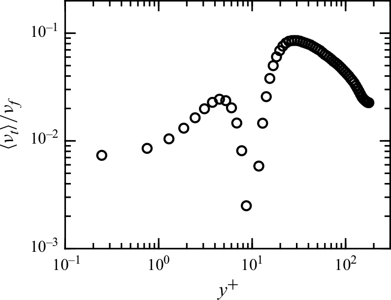
Figure 16 shows the ratio of the mean eddy viscosity,
 $\langle \nu _t \rangle$
, to the molecular viscosity,
$\langle \nu _t \rangle$
, to the molecular viscosity,
 $\nu _f$
, along the wall-normal direction. The mean eddy viscosity is computed by averaging
$\nu _f$
, along the wall-normal direction. The mean eddy viscosity is computed by averaging
 $\nu _t (\mathbf{x},t)$
over the wall-parallel (
$\nu _t (\mathbf{x},t)$
over the wall-parallel (
 $x$
-
$x$
-
 $z$
) plane and time. Profiles of
$z$
) plane and time. Profiles of
 $\langle \nu _t \rangle / \nu _f$
for other cases are not shown, as they show no noticeable differences compared with figure 16. The ratio remains significantly smaller than unity throughout the channel, with a peak value of
$\langle \nu _t \rangle / \nu _f$
for other cases are not shown, as they show no noticeable differences compared with figure 16. The ratio remains significantly smaller than unity throughout the channel, with a peak value of
 $ \langle \nu _t \rangle _{{max}} / \nu _f = 8.5 \times 10^{-2}$
. This suggests that the unresolved Reynolds stress,
$ \langle \nu _t \rangle _{{max}} / \nu _f = 8.5 \times 10^{-2}$
. This suggests that the unresolved Reynolds stress,
 $\mathcal{F}_{u}$
, is negligible compared with the resolved stress,
$\mathcal{F}_{u}$
, is negligible compared with the resolved stress,
 $\overline {\boldsymbol{\tau }}^*$
, and is thus omitted in this study.
$\overline {\boldsymbol{\tau }}^*$
, and is thus omitted in this study.
The insignificant Reynolds stress can be attributed to the fact that the filter size,
 $\delta _F$
, is small compared with the size of near-wall coherent structures. In this study, there is a significant scale separation between the particle size (
$\delta _F$
, is small compared with the size of near-wall coherent structures. In this study, there is a significant scale separation between the particle size (
 ${d}_p=0.36 \delta _\nu$
) and the turbulent coherent structures. For example, the core size of quasi-streamwise vortices in the
${d}_p=0.36 \delta _\nu$
) and the turbulent coherent structures. For example, the core size of quasi-streamwise vortices in the
 $x-z$
plane is typically around
$x-z$
plane is typically around
 $O(10) \delta _\nu$
and even longer in the streamwise direction (Marchioli & Soldati Reference Marchioli and Soldati2002). Consequently, even though the filter size is relatively large compared with the particle diameter (
$O(10) \delta _\nu$
and even longer in the streamwise direction (Marchioli & Soldati Reference Marchioli and Soldati2002). Consequently, even though the filter size is relatively large compared with the particle diameter (
 $\delta _F=8{d}_p$
), the near-wall coherent structures remain resolved.
$\delta _F=8{d}_p$
), the near-wall coherent structures remain resolved.
We now address the closure of
 $\boldsymbol{\tau }_{\mu }$
. As expressed in (B12),
$\boldsymbol{\tau }_{\mu }$
. As expressed in (B12),
 $\boldsymbol{\tau }_{\mu }$
arises from the filtering of the velocity gradient. In previous studies,
$\boldsymbol{\tau }_{\mu }$
arises from the filtering of the velocity gradient. In previous studies,
 $\boldsymbol{\tau }_{\mu }$
was often modelled by introducing an effective viscosity
$\boldsymbol{\tau }_{\mu }$
was often modelled by introducing an effective viscosity
 $\mu ^*$
, which depends on the particle volume fraction, as seen in both dilute and dense particulate flows (Zhang & Prosperetti Reference Zhang and Prosperetti1997; Patankar & Joseph Reference Patankar and Joseph2001). To leading order, the relative change in viscosity scales with
$\mu ^*$
, which depends on the particle volume fraction, as seen in both dilute and dense particulate flows (Zhang & Prosperetti Reference Zhang and Prosperetti1997; Patankar & Joseph Reference Patankar and Joseph2001). To leading order, the relative change in viscosity scales with
 $\alpha _p$
. In this work, given the low particle concentration, the change of
$\alpha _p$
. In this work, given the low particle concentration, the change of
 $\mu ^*$
is expected to be small. As a result,
$\mu ^*$
is expected to be small. As a result,
 $\boldsymbol{\tau }_{\mu }$
is also omitted. Finally, by omitting both
$\boldsymbol{\tau }_{\mu }$
is also omitted. Finally, by omitting both
 $\mathcal{F}_u$
and
$\mathcal{F}_u$
and
 $\boldsymbol{\tau }_{\mu }$
, (B17) becomes
$\boldsymbol{\tau }_{\mu }$
, (B17) becomes
 \begin{equation} \frac {\partial }{\partial t}(\alpha _f \overline {\mathbf{u}}_f) + \boldsymbol{\nabla} \cdot (\alpha _f \overline {\mathbf{u}}_f \otimes \overline {\mathbf{u}}_f)= \frac {1}{\rho _f} (\boldsymbol{\nabla} \cdot \overline {\boldsymbol{\tau }}^* -\mathcal{F}_P). \end{equation}
Equations (B7) and (B22) are in fact equivalent to (2.2) without the forcing term. For simplicity, the symbols representing volume filtering are omitted in the main text.
Appendix C. Importance of the lift force and the lubrication force
In this study, both the lift force and the lubrication force are omitted due to their negligible impacts under the given simulation conditions. The reasons and justifications are provided below.
C.1 Lift force
The extended expression of Saffman lift force is used to evaluate the importance of lift force in this study. The magnitude of the lift force is
 \begin{align} F_l=\frac {9J}{\pi } \mu _f ({d}_p/2)^2 u_{slip} (G/\nu _f)^{1/2}. \end{align}
Here,
 $J$
is a coefficient to be determined,
$J$
is a coefficient to be determined,
 $\mu _f$
and
$\mu _f$
and
 $\nu _f$
are the dynamic and kinematic viscosity of the fluid,
$\nu _f$
are the dynamic and kinematic viscosity of the fluid,
 ${d}_p$
is the particle diameter,
${d}_p$
is the particle diameter,
 $u_{slip}$
is the particle slip velocity in the streamwise direction and
$u_{slip}$
is the particle slip velocity in the streamwise direction and
 $G$
is the fluid shear rate. The magnitude of drag force can be written as
$G$
is the fluid shear rate. The magnitude of drag force can be written as
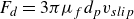 $F_d=3 \pi \mu _f {d}_p v_{slip}$
, where
$F_d=3 \pi \mu _f {d}_p v_{slip}$
, where
 $v_{slip}$
is the particle slip velocity in the wall-normal direction. The ratio between the force magnitudes can then be written as
$v_{slip}$
is the particle slip velocity in the wall-normal direction. The ratio between the force magnitudes can then be written as
 \begin{align} \frac {F_l}{F_d}=\frac {3J}{4\pi ^2}Re_G^{1/2} \frac {u_{slip}}{v_{slip}}, \end{align}
where
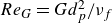 $Re_G=G {d}_p^2/\nu _f$
is the particle shear Reynolds number. In this study, the fluid shear rate is estimated using the inner scales as
$Re_G=G {d}_p^2/\nu _f$
is the particle shear Reynolds number. In this study, the fluid shear rate is estimated using the inner scales as
 $G=1/\tau _{\nu }=u_\tau ^2/\nu _f$
, which leads to
$G=1/\tau _{\nu }=u_\tau ^2/\nu _f$
, which leads to
 $Re_G=0.13$
. The particle Reynolds number is calculated as
$Re_G=0.13$
. The particle Reynolds number is calculated as
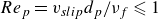 $Re_p=v_{slip}{d}_p/\nu _f \leqslant 1$
. Based on the values of both
$Re_p=v_{slip}{d}_p/\nu _f \leqslant 1$
. Based on the values of both
 $Re_p$
and
$Re_p$
and
 $Re_G$
, the coefficient
$Re_G$
, the coefficient
 $J$
is determined to be
$J$
is determined to be
 $J \leqslant 2.172$
using the fitting equation proposed by Mei (Reference Mei1992). Moreover, the velocity ratio
$J \leqslant 2.172$
using the fitting equation proposed by Mei (Reference Mei1992). Moreover, the velocity ratio
 $u_{slip}/v_{slip}$
ranges approximately from 2 to 5 in the simulations. Finally, the force ratio is computed as
$u_{slip}/v_{slip}$
ranges approximately from 2 to 5 in the simulations. Finally, the force ratio is computed as
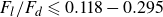 $F_l/F_d \leqslant 0.118-0.295$
, which suggests that the influence of the lift force is minor compared with the drag force. We therefore neglect the lift force in this study.
$F_l/F_d \leqslant 0.118-0.295$
, which suggests that the influence of the lift force is minor compared with the drag force. We therefore neglect the lift force in this study.
C.2 Short-range lubrication force
In this study, the lubrication force is negligible because of the large particle-to-air density ratio (
 $\rho _p/\rho _f \sim O(10^3)$
). In other multiphase flow systems, such as bubble flows (
$\rho _p/\rho _f \sim O(10^3)$
). In other multiphase flow systems, such as bubble flows (
 $\rho _p/\rho _f \sim O(10^{-3})$
) or colloidal systems (
$\rho _p/\rho _f \sim O(10^{-3})$
) or colloidal systems (
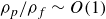 $\rho _p/\rho _f \sim O(1)$
), the lubrication force will be substantial and must be considered.
$\rho _p/\rho _f \sim O(1)$
), the lubrication force will be substantial and must be considered.
To confirm this argument, the influence of lubrication force can be estimated as follows. For a pair of particles (
 $i$
and
$i$
and
 $j$
) approaching each other, the lubrication force has been derived by Marshall (Reference Marshall2011), which is given as
$j$
) approaching each other, the lubrication force has been derived by Marshall (Reference Marshall2011), which is given as
 \begin{align} F_{lub}=\frac {3 \pi \mu _f r_p^2}{2h} \left ( -\frac {\textrm{d}h}{\textrm{d}t} \right ), \end{align}
where
 $h=|\mathbf{x}_i-\mathbf{x}_j|-({d}_{p,i}+{d}_{p,j})/2$
is the gap between the surfaces of the two particles, and
$h=|\mathbf{x}_i-\mathbf{x}_j|-({d}_{p,i}+{d}_{p,j})/2$
is the gap between the surfaces of the two particles, and
 $(-\textrm{d}h/\textrm{d}t)$
is the radial approaching velocity. As two particles approach each other, they need to squeeze out the fluid film in between in order to collide, and the associated energy barrier is
$(-\textrm{d}h/\textrm{d}t)$
is the radial approaching velocity. As two particles approach each other, they need to squeeze out the fluid film in between in order to collide, and the associated energy barrier is
 \begin{align} E_{lub}=\int _{h_{min}}^{h_{max}} F_{lub} \textrm{d}h. \end{align}
Here,
 $h_{max}$
is the initial separation distance below which the short-range lubrication effect becomes important, and
$h_{max}$
is the initial separation distance below which the short-range lubrication effect becomes important, and
 $h_{min}$
represents the minimum separation distance between colliding particles. According to Barnocky & Davis (Reference Barnocky and Davis1989), the fluid density and viscosity within the contact region can increase substantially due to the high pressure in the gap, exhibiting solid-like behaviour and thereby imposing a lower limit on
$h_{min}$
represents the minimum separation distance between colliding particles. According to Barnocky & Davis (Reference Barnocky and Davis1989), the fluid density and viscosity within the contact region can increase substantially due to the high pressure in the gap, exhibiting solid-like behaviour and thereby imposing a lower limit on
 $h_{min}$
. In addition, surface roughness further constrains
$h_{min}$
. In addition, surface roughness further constrains
 $h_{min}$
due to the presence of finite-size asperities on the particle surfaces. Here, we set
$h_{min}$
due to the presence of finite-size asperities on the particle surfaces. Here, we set
 $h_{max}=0.01 r_p$
and
$h_{max}=0.01 r_p$
and
 $h_{min}= 5 \times 10^{-5} r_p$
with
$h_{min}= 5 \times 10^{-5} r_p$
with
 $r_p$
being the particle radius, which yields collision outcomes that show reasonable agreement with experimental data (Yang & Hunt Reference Yang and Hunt2006; Marshall Reference Marshall2011). By taking the initial approaching velocity
$r_p$
being the particle radius, which yields collision outcomes that show reasonable agreement with experimental data (Yang & Hunt Reference Yang and Hunt2006; Marshall Reference Marshall2011). By taking the initial approaching velocity
 $v_{init} \geqslant |\textrm{d}h/\textrm{d}t|$
out of the integral, the upper limit of the energy barrier becomes
$v_{init} \geqslant |\textrm{d}h/\textrm{d}t|$
out of the integral, the upper limit of the energy barrier becomes
 \begin{align} E_{lub}=\frac {3}{2} \pi \mu _f r_p^2 v_{init} \ln {\left ( \frac {h_{max}}{h_{min}} \right )}. \end{align}
Meanwhile, the driving force of an interparticle collision is the relative kinetic energy
 $E_{kin}=M v_{init}^2/2$
, where
$E_{kin}=M v_{init}^2/2$
, where
 $M=m/2$
is the effective mass of a two-particle system. Finally, the significance of lubrication is quantified by the energy ratio
$M=m/2$
is the effective mass of a two-particle system. Finally, the significance of lubrication is quantified by the energy ratio
 \begin{align} \frac {E_{lub}}{E_{kin}} = \frac {9 \mu _f}{\rho _p {d}_p v_{init}} \ln {\left ( \frac {h_{max}}{h_{min}} \right )}. \end{align}
In our simulations,
 $v_{init}$
is calculated as the mean radial relative velocity between a pair of approaching particles with a gap
$v_{init}$
is calculated as the mean radial relative velocity between a pair of approaching particles with a gap
 $h \in [0.009r_p, 0.011r_p]$
. The resulting values are
$h \in [0.009r_p, 0.011r_p]$
. The resulting values are
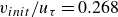 $v_{init}/u_{\tau }=0.268$
for
$v_{init}/u_{\tau }=0.268$
for
 $St^+=32$
and
$St^+=32$
and
 $v_{init}/u_{\tau }=3.382$
for
$v_{init}/u_{\tau }=3.382$
for
 $St^+=133$
. Plugging in the simulation parameters then yields
$St^+=133$
. Plugging in the simulation parameters then yields
 $E_{lub}/E_{kin}=0.110$
for
$E_{lub}/E_{kin}=0.110$
for
 $St^+=32$
and
$St^+=32$
and
 $E_{lub}/E_{kin}=0.002$
for
$E_{lub}/E_{kin}=0.002$
for
 $St^+=133$
. The small energy ratios suggest that the lubrication force has a weak effect on interparticle motions during collisions. Therefore, the lubrication force is omitted in the simulations.
$St^+=133$
. The small energy ratios suggest that the lubrication force has a weak effect on interparticle motions during collisions. Therefore, the lubrication force is omitted in the simulations.
Appendix D. Influence of interpolation scheme
The order of the interpolation scheme can indeed influence the accuracy of high-order derivatives of velocity. However, in this study, we only consider the drag force, which does not require higher-order derivatives of velocity at the particle position. Since the calculation of drag force depends solely on the interpolation of fluid velocity, the second-order trilinear interpolation is sufficient. To check the effect of interpolation order, the same test case (
 $St^+=32$
,
$St^+=32$
,
 $q=0 \ \textrm{C}$
) was run using three different interpolation schemes: second-order trilinear interpolation (Trilinear), fourth-order Lagrangian interpolation (Lag4) and eighth-order Lagrangian interpolation (Lag8). Comparisons of the steady-state statistics are presented in figure 17. As no significant differences were observed among the results obtained with different interpolation schemes, the accuracy of trilinear interpolation is considered adequate for this study.
$q=0 \ \textrm{C}$
) was run using three different interpolation schemes: second-order trilinear interpolation (Trilinear), fourth-order Lagrangian interpolation (Lag4) and eighth-order Lagrangian interpolation (Lag8). Comparisons of the steady-state statistics are presented in figure 17. As no significant differences were observed among the results obtained with different interpolation schemes, the accuracy of trilinear interpolation is considered adequate for this study.
Comparison of (a) normalised wall-normal particle concentration
 $C/C_0$
, (b) mean streamwise particle velocity and (c) r.m.s. of wall-normal particle fluctuation velocity using different interpolation schemes for the case with
$C/C_0$
, (b) mean streamwise particle velocity and (c) r.m.s. of wall-normal particle fluctuation velocity using different interpolation schemes for the case with
 $St^+=32$
and
$St^+=32$
and
 $q=0 \ \textrm{C}$
.
$q=0 \ \textrm{C}$
.

Appendix E. Undisturbed fluid velocity in drag force calculation
In this section, we discuss the error caused by self-induced disturbance in drag force in two-way coupled simulations. By definition, the Stokes drag on a target particle at
 $x_p$
is evaluated based on the slip velocity
$x_p$
is evaluated based on the slip velocity
 $(\tilde {u}_f(x_p)-v_p)$
, where
$(\tilde {u}_f(x_p)-v_p)$
, where
 $\tilde {u}_f(x_p)$
is the undisturbed fluid velocity at the particle location. However, in two-way coupled simulations, the feedback force from the target particle itself perturbs surrounding fluid flow. As a result, the local fluid velocity,
$\tilde {u}_f(x_p)$
is the undisturbed fluid velocity at the particle location. However, in two-way coupled simulations, the feedback force from the target particle itself perturbs surrounding fluid flow. As a result, the local fluid velocity,
 $u_f(x_p) (\neq \tilde {u}_f(x_p))$
, is disturbed, leading to an underestimated slip velocity and, consequently, a reduced drag force.
$u_f(x_p) (\neq \tilde {u}_f(x_p))$
, is disturbed, leading to an underestimated slip velocity and, consequently, a reduced drag force.
The error in drag force depends on the ratio of the particle size to the length scale of the projection scheme used to map particle disturbances onto the grid mesh. In standard Eulerian–Lagrangian simulations, where particle feedback forces are typically distributed to nearby grid points, the error scales as
 $O({d}_p/\Delta x)$
, where
$O({d}_p/\Delta x)$
, where
 $\Delta x$
is the grid spacing (Horwitz & Mani Reference Horwitz and Mani2016). In this study, however, we distribute the particle volume fraction and the feedback force using a Gaussian filter
$\Delta x$
is the grid spacing (Horwitz & Mani Reference Horwitz and Mani2016). In this study, however, we distribute the particle volume fraction and the feedback force using a Gaussian filter
 $G_F(r)$
with a filter length
$G_F(r)$
with a filter length
 $\delta _F=8 {d}_p$
((2.8a
) and (2.8b
)). As the projection length scale becomes no smaller than
$\delta _F=8 {d}_p$
((2.8a
) and (2.8b
)). As the projection length scale becomes no smaller than
 $\delta _F$
, the upper limit of the error is expected to depend on the new size ratio
$\delta _F$
, the upper limit of the error is expected to depend on the new size ratio
 ${d}_p/\delta _f$
.
${d}_p/\delta _f$
.
Regarding the VFEL framework used in the present study, Ireland & Desjardins (Reference Ireland and Desjardins2017) discussed the corrections of both fluid volume fraction (
 $\zeta _{\alpha _f}=\tilde {\alpha }_f- \alpha _f$
) and fluid velocity (
$\zeta _{\alpha _f}=\tilde {\alpha }_f- \alpha _f$
) and fluid velocity (
 $\zeta _{u_f}=\tilde {u}_f-u_f$
). By considering the case of the steady Stokes flow around a particle, the corrections can be given by
$\zeta _{u_f}=\tilde {u}_f-u_f$
). By considering the case of the steady Stokes flow around a particle, the corrections can be given by
 \begin{equation} \zeta _{\alpha _f}=\tilde {\alpha }_f-\alpha _f=\textrm{erf}\left (\frac {1}{\sqrt {2} \hat {\sigma }_c}\right )-\frac {\sqrt {2/\pi }}{\hat {\sigma }_c}\textrm{exp}\left ( -\frac {1}{2 \hat {\sigma }_c^2 }\right ), \end{equation}
 \begin{equation} \frac {\zeta _{u_f}}{U}=\frac {\left (\frac {1}{\sqrt {2} \hat {\sigma }_c}\right )\textrm{exp}\left ( -\frac {1}{2 \hat {\sigma }_c^2 }\right )}{1-\textrm{erf}\left (\frac {1}{\sqrt {2} \hat {\sigma }_c}\right ) + \frac {\sqrt {2/\pi }}{\hat {\sigma }_c}\textrm{exp}\left ( -\frac {1}{2 \hat {\sigma }_c^2 }\right )}. \end{equation}
Here,
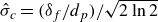 $\hat {\sigma }_c=(\delta _f/{d}_p)/\sqrt {2\ln {2}}$
, and
$\hat {\sigma }_c=(\delta _f/{d}_p)/\sqrt {2\ln {2}}$
, and
 $U$
is the slip velocity in the Stokes flow problem. We would like to note that, in cases with high particle volume fraction, the drag force model typically accounts for the local fluid volume fraction (
$U$
is the slip velocity in the Stokes flow problem. We would like to note that, in cases with high particle volume fraction, the drag force model typically accounts for the local fluid volume fraction (
 $\alpha _f=1-\alpha _p$
). Consequently, the self-induced disturbance of fluid volume fraction (
$\alpha _f=1-\alpha _p$
). Consequently, the self-induced disturbance of fluid volume fraction (
 $\zeta _{\alpha _f}$
) could also influence the drag force in two-way coupled simulations. However, in the present work, the mean particle volume fraction is low (
$\zeta _{\alpha _f}$
) could also influence the drag force in two-way coupled simulations. However, in the present work, the mean particle volume fraction is low (
 $\overline {\alpha }_p \sim 10^{-6}$
), so the drag force model does not include corrections for the influence of
$\overline {\alpha }_p \sim 10^{-6}$
), so the drag force model does not include corrections for the influence of
 $\alpha _f$
. Furthermore, the particle Reynolds number in the current study satisfies
$\alpha _f$
. Furthermore, the particle Reynolds number in the current study satisfies
 $Re_p \leqslant 1$
. As a result, although the velocity correction is derived based on Stokes flow, it provides a reasonable first-order approximation of the velocity correction. Using the filter length
$Re_p \leqslant 1$
. As a result, although the velocity correction is derived based on Stokes flow, it provides a reasonable first-order approximation of the velocity correction. Using the filter length
 $\delta _f=8 {d}_p$
then yields
$\delta _f=8 {d}_p$
then yields
 $\zeta _{\alpha _f}=8.42 \times 10^{-3}$
and
$\zeta _{\alpha _f}=8.42 \times 10^{-3}$
and
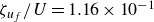 $\zeta _{u_f}/U=1.16 \times 10^{-1}$
. This indicates that the error in the drag force due to self-induced velocity disturbance is secondary. To further verify this statement, we apply the fluid velocity correction scheme proposed in Ireland & Desjardins (Reference Ireland and Desjardins2017) with
$\zeta _{u_f}/U=1.16 \times 10^{-1}$
. This indicates that the error in the drag force due to self-induced velocity disturbance is secondary. To further verify this statement, we apply the fluid velocity correction scheme proposed in Ireland & Desjardins (Reference Ireland and Desjardins2017) with
 $\hat {\zeta }_{u_f}=\zeta _{u_f}/U=1.16 \times 10^{-1}$
, which reads
$\hat {\zeta }_{u_f}=\zeta _{u_f}/U=1.16 \times 10^{-1}$
, which reads
 \begin{equation} \tilde {\mathbf{u}}_f=\frac {\mathbf{u}_f-\mathbf{v}_p \hat {\zeta }_{u_f}}{1-\hat {\zeta }_{u_f}}, \end{equation}
to two test cases with different Stokes numbers (
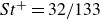 $St^+=32/133$
) and zero particle charge.
$St^+=32/133$
) and zero particle charge.
Comparison of (a) normalised wall-normal particle concentration
 $C/C_0$
, (b) mean streamwise particle velocity
$C/C_0$
, (b) mean streamwise particle velocity
 $v_{px}^+$
and (c) r.m.s. of wall-normal particle velocity
$v_{px}^+$
and (c) r.m.s. of wall-normal particle velocity
 $v_{py,rms}^+$
between cases without (w/o) and with (w) the velocity correction.
$v_{py,rms}^+$
between cases without (w/o) and with (w) the velocity correction.

Figure 18 compares typical particle statistics between cases with and without the velocity correction. The r.m.s. of the wall-normal particle velocity, shown in figure 18(c), exhibits a slight increase when the velocity correction scheme is applied. The increase in
 $v_{py,rms}^+$
for
$v_{py,rms}^+$
for
 $St^+=133$
is also found to be larger than that for
$St^+=133$
is also found to be larger than that for
 $St^+=32$
. These changes are reasonable, as the fluid drag force calculated using the undisturbed fluid velocity is larger, making inertial particles more responsive to background turbulence fluctuations and, therefore, more energetic. Moreover, particles with larger inertia (
$St^+=32$
. These changes are reasonable, as the fluid drag force calculated using the undisturbed fluid velocity is larger, making inertial particles more responsive to background turbulence fluctuations and, therefore, more energetic. Moreover, particles with larger inertia (
 $St^+=133$
) generally experience more significant slip velocities, making their statistics more sensitive to velocity correction compared with those with moderate inertia
$St^+=133$
) generally experience more significant slip velocities, making their statistics more sensitive to velocity correction compared with those with moderate inertia
 $St^+=32$
. However, both the wall-normal concentration (figure 18
a) and the mean streamwise particle velocity (figure 18b) show no noticeable differences. We thus conclude that errors in drag force calculation do not significantly affect particle transport under current conditions, so the main conclusions of this work remain valid.
$St^+=32$
. However, both the wall-normal concentration (figure 18
a) and the mean streamwise particle velocity (figure 18b) show no noticeable differences. We thus conclude that errors in drag force calculation do not significantly affect particle transport under current conditions, so the main conclusions of this work remain valid.
Appendix F. Validation of the electrostatic computation
To validate the PP electrostatic force, we consider the Coulomb force acting on
 $N_{\textrm{p}}=5000$
particles in the three-dimensional periodic box with a side length of
$N_{\textrm{p}}=5000$
particles in the three-dimensional periodic box with a side length of
 $L=2 \pi$
. Half of the particles carry a nominal positive charge
$L=2 \pi$
. Half of the particles carry a nominal positive charge
 $q=1$
, while the others carry a nominal negative charge
$q=1$
, while the others carry a nominal negative charge
 $q=-1$
. For this charge-neutral system, the exact Coulomb force acting on particle
$q=-1$
. For this charge-neutral system, the exact Coulomb force acting on particle
 $i$
can be computed by the standard Ewald summation (Deserno & Holm Reference Deserno and Holm1998) as
$i$
can be computed by the standard Ewald summation (Deserno & Holm Reference Deserno and Holm1998) as
 \begin{align} \boldsymbol {F}^{{E,Ewald}}_i = \boldsymbol {F}^{(r)}_i + \boldsymbol {F}^{(k)}_i + \boldsymbol {F}^{(d)}_i, \end{align}
where the contribution from the real space
 $\boldsymbol {F}^{\textrm{(r)}}_i$
, the Fourier space
$\boldsymbol {F}^{\textrm{(r)}}_i$
, the Fourier space
 $\boldsymbol {F}^{\textrm{(k)}}_i$
and the dipole correction
$\boldsymbol {F}^{\textrm{(k)}}_i$
and the dipole correction
 $\boldsymbol {F}^{\textrm{(d)}}_i$
are given as
$\boldsymbol {F}^{\textrm{(d)}}_i$
are given as
 \begin{align} \boldsymbol {F}^{\textrm{(r)}}_i & = \frac {q_i}{4 \pi \varepsilon _0} \sum _j q_j \sum _{\boldsymbol {m} \in \mathbb{Z}^3}^{\prime } \left ( \frac {2 \alpha }{\sqrt {\pi }} \textrm{exp} \left ( -\alpha ^2 |\boldsymbol {r}_{ij} + \boldsymbol {m}L|^2 \right )\right. \notag\\ &\quad\left. + \frac {\textrm{erfc} ( \alpha |\boldsymbol {r}_{ij} +\boldsymbol {m}L| )}{|\boldsymbol {r}_{ij} +\boldsymbol {m}L|} \right ) \frac {\boldsymbol {r}_{ij} +\boldsymbol {m}L}{|\boldsymbol {r}_{ij} +\boldsymbol {m}L|^2}, \end{align}
 \begin{align} \boldsymbol {F}^{\textrm{(k)}}_i & = \frac {q_i}{4 \pi \varepsilon _0 L^3} \sum _j q_j \sum _{\boldsymbol {k} \neq \boldsymbol {0}} \frac {4 \pi \boldsymbol {k}}{k^2} \textrm{exp} \left ( -\frac {k^2}{4 \alpha ^2} \right ) \sin {(\boldsymbol {k} \cdot \boldsymbol {r}_{ij})}, \end{align}
 \begin{align} \boldsymbol {F}^{\textrm{(d)}}_i & = -\frac {q_i}{\varepsilon _0 (1+2 \varepsilon ^{\prime })L^3} \sum _j q_j \boldsymbol {x}_j. \end{align}
Here,
 $\alpha$
is the Ewald parameter,
$\alpha$
is the Ewald parameter,
 $\textrm{erfc}$
is the complementary error function, and
$\textrm{erfc}$
is the complementary error function, and
 $\varepsilon ^{\prime }=1$
is the relative dielectric constant of the surrounding medium.
$\varepsilon ^{\prime }=1$
is the relative dielectric constant of the surrounding medium.
Table 6 lists the parameters used in Ewald summation. The dimensionless product
 $\alpha r_{\textrm{C}}$
is set to
$\alpha r_{\textrm{C}}$
is set to
 $\pi$
to ensure high accuracy in both real and Fourier spaces. The cutoff radius (
$\pi$
to ensure high accuracy in both real and Fourier spaces. The cutoff radius (
 $r_{\textrm{C}}$
) and wavenumber (
$r_{\textrm{C}}$
) and wavenumber (
 $k_{\textrm{C}}$
) in real and Fourier spaces, respectively, are then determined by
$k_{\textrm{C}}$
) in real and Fourier spaces, respectively, are then determined by
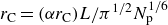 $r_{\textrm{C}}=(\alpha r_{\textrm{C}}) L/\pi ^{1/2}N_{\textrm{p}}^{1/6}$
and
$r_{\textrm{C}}=(\alpha r_{\textrm{C}}) L/\pi ^{1/2}N_{\textrm{p}}^{1/6}$
and
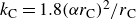 $k_{\textrm{C}} = 1.8 (\alpha r_{\textrm{C}})^2/r_{\textrm{C}}$
to balance the computation cost of
$k_{\textrm{C}} = 1.8 (\alpha r_{\textrm{C}})^2/r_{\textrm{C}}$
to balance the computation cost of
 $\boldsymbol {F}^{\textrm{(r)}}_i$
and
$\boldsymbol {F}^{\textrm{(r)}}_i$
and
 $\boldsymbol {F}^{\textrm{(k)}}_i$
(Fincham Reference Fincham1994). Due to the high accuracy of Ewald summation,
$\boldsymbol {F}^{\textrm{(k)}}_i$
(Fincham Reference Fincham1994). Due to the high accuracy of Ewald summation,
 $\boldsymbol {F}^{{E,Ewald}}_i$
is used as the reference electrostatic force acting on the particles. In § 2.6.1, the P
$\boldsymbol {F}^{{E,Ewald}}_i$
is used as the reference electrostatic force acting on the particles. In § 2.6.1, the P
 $^3$
M method is also employed to compute the electrostatic force under the same conditions. The relative error,
$^3$
M method is also employed to compute the electrostatic force under the same conditions. The relative error,
 $\epsilon _r$
, is then evaluated using (2.20). With the minimum
$\epsilon _r$
, is then evaluated using (2.20). With the minimum
 $\epsilon _r\lt 1\,\%$
(figure 5
d), the P
$\epsilon _r\lt 1\,\%$
(figure 5
d), the P
 $^3$
M method is considered accurate for computing the PP electrostatic force.
$^3$
M method is considered accurate for computing the PP electrostatic force.
Dimensionless parameters for Ewald summation.
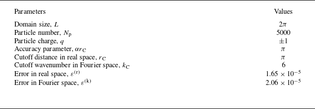
Appendix G. Derivation of the wall-normal particle concentration profile
In this appendix, the wall-normal particle concentration profile is derived following Johnson et al. (2020). Define
 $f(y,v_{py};t)$
as the probability density function of particles in the phase space
$f(y,v_{py};t)$
as the probability density function of particles in the phase space
 $(y,v_{py})$
at time
$(y,v_{py})$
at time
 $t$
, where
$t$
, where
 $y$
is the wall-normal particle location and
$y$
is the wall-normal particle location and
 $v_{py}$
is the wall-normal particle velocity. By definition, the wall-normal particle concentration profile
$v_{py}$
is the wall-normal particle velocity. By definition, the wall-normal particle concentration profile
 $C(y;t)$
can be directly determined from
$C(y;t)$
can be directly determined from
 $f(y,v_{py};t)$
as
$f(y,v_{py};t)$
as
 \begin{equation} C(y;t)=C_0 \int _{-\infty }^{\infty } f(y,v_{py};t) \textrm{d} v_{py}, \end{equation}
where
 $C_0$
is the domain-averaged particle concentration. The governing equation of
$C_0$
is the domain-averaged particle concentration. The governing equation of
 $f$
in the phase space is
$f$
in the phase space is
 \begin{equation} \frac {\partial f}{\partial t} + \frac {\partial \left ( v_{py} \cdot f \right )}{\partial y} + \frac {\partial \left (a_{py} \cdot f\right )}{\partial v_{py}} = \dot {f}_{C}. \end{equation}
Here,
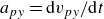 $a_{py}=\textrm{d} v_{py}/\textrm{d} t$
is the wall-normal particle acceleration.
$a_{py}=\textrm{d} v_{py}/\textrm{d} t$
is the wall-normal particle acceleration.
 $\dot {f}_{C}$
is the change of
$\dot {f}_{C}$
is the change of
 $f$
due to collisions. Two simplifications can be made here: (i) as particles are assumed to be elastic in this study, both particle mass and momentum are conserved in each collision, which leads to
$f$
due to collisions. Two simplifications can be made here: (i) as particles are assumed to be elastic in this study, both particle mass and momentum are conserved in each collision, which leads to
 $\dot {f}_{C}=0$
; (ii) when the particle field reaches equilibrium,
$\dot {f}_{C}=0$
; (ii) when the particle field reaches equilibrium,
 $f$
is time-independent, i.e.
$f$
is time-independent, i.e.
 ${\partial f}/{\partial t}=0$
. By multiplying the simplified (G2) by
${\partial f}/{\partial t}=0$
. By multiplying the simplified (G2) by
 $v_{py}$
and
$v_{py}$
and
 $C_0$
, and then integrating from
$C_0$
, and then integrating from
 $v_{py}=-\infty$
to
$v_{py}=-\infty$
to
 $v_{py}=\infty$
, the momentum conservation equation can be written as
$v_{py}=\infty$
, the momentum conservation equation can be written as
 \begin{equation} \frac {\textrm{d}}{\textrm{d} y} \left ( \langle v_{py}^2 | y \rangle C \right ) - \langle a_{py} | y \rangle C = 0. \end{equation}
Here, the notation
 $\langle *|y \rangle$
denotes the ensemble average of quantities conditioned at the wall-normal location
$\langle *|y \rangle$
denotes the ensemble average of quantities conditioned at the wall-normal location
 $y$
. For a particle located at
$y$
. For a particle located at
 $y$
, its wall-normal acceleration due to drag and electrostatic force is
$y$
, its wall-normal acceleration due to drag and electrostatic force is
 \begin{equation} a_{py}=\frac {f_I \left (u_{fy}-v_{py} \right )}{\tau _p}+\frac {qE_y}{m}, \end{equation}
where
 $u_{fy}$
and
$u_{fy}$
and
 $E_y$
are the wall-normal components of the fluid velocity and the electric field. Plugging (G4) into (G3) and integrating along the wall-normal direction then yields the wall-normal particle concentration profile
$E_y$
are the wall-normal components of the fluid velocity and the electric field. Plugging (G4) into (G3) and integrating along the wall-normal direction then yields the wall-normal particle concentration profile
 \begin{equation} \begin{aligned} C(y)= \mathcal{C}^{\prime } \textrm{exp} \Bigg ( & -\int _0^y \frac {\textrm{d} \ln { \langle v_{py}^2 | \eta \rangle }}{\textrm{d} \eta } \textrm{d} \eta + \frac {1}{\tau _p} \int _0^y \frac {\langle f_I (u_{fy}-v_{py}) |\eta \rangle }{\langle v_{py}^2 |\eta \rangle } \textrm{d} \eta \\ & + \frac {q}{m} \int _0^y \frac {\langle E_{y} | \eta \rangle }{\langle v_{py}^2 | \eta \rangle } \textrm{d} \eta \Bigg ), \end{aligned} \end{equation}
where
 $\mathcal{C}^{\prime }$
is an unknown coefficient that can be determined from particle mass conservation.
$\mathcal{C}^{\prime }$
is an unknown coefficient that can be determined from particle mass conservation.


 Open access