


1. Introduction
Inertial measurement units (IMUs) are important sensors in the context of state estimation. A popular approach in robotics is to treat IMU measurements as inputs to a motion model and then to numerically integrate the motion model to form relative motion factors between pairs of estimation times in a process known as preintegration [Reference Lupton and Sukkarieh1–Reference Brossard, Barrau, Chauchat and Bonnabel3]. In this paper, we investigate the treatment of IMUs as a measurement of the state using continuous-time state estimation with a Gaussian process motion prior. We compare treating an IMU as an input versus a measurement on a simple 1D simulation problem. We then test our approach to lidar-inertial odometry using a simulated environment and compare to a baseline that represents the IMU-as-input approach. Finally, we provide experimental results for our lidar-inertial odometry on the Newer College Dataset.
Preintegration was initially devised as a method to avoid having to estimate the state at each measurement time in (sliding-window) batch trajectory estimation. We will show that by employing our continuous-time estimation techniques, we can achieve the same big-O complexity as classic preintegration, which is linear in the number of measurements. The contributions of this work are as follows:
-
• We provide a detailed comparison of treating an IMU as an input to a motion model versus as a measurement of the state on a 1D simulation problem. Such a comparison has not been previously presented in the literature.
-
• We show how to perform preintegration using heterogeneous factors (a combination of binary and unary factors) using continuous-time state estimation. To our knowledge, this has not been shown before in the literature.
-
• We present our novel approach to lidar-inertial odometry using a Singer prior which includes body-centric acceleration in the state. We provide experimental results on the Newer College Dataset and on a custom simulated dataset. On the Newer College Dataset, we demonstrate state-of-the art performance.
2. Related work
Lupton and Sukkarieh [Reference Lupton and Sukkarieh1] were the first to show that a temporal window of inertial measurements could be summarized using a single relative motion factor in a method known as preintegration. Forster et al. [Reference Forster, Carlone, Dellaert and Scaramuzza2] then showed how to perform preintegration on the manifold $SO(3)$
. Subsequently, Brossard et al. [Reference Brossard, Barrau, Chauchat and Bonnabel3] demonstrated how to perform preintegration on the manifold of extended poses
$SO(3)$
. Subsequently, Brossard et al. [Reference Brossard, Barrau, Chauchat and Bonnabel3] demonstrated how to perform preintegration on the manifold of extended poses $SE_2(3)$
, showing that this approach captures the uncertainty resulting from IMU measurements more consistently than
$SE_2(3)$
, showing that this approach captures the uncertainty resulting from IMU measurements more consistently than $SO(3) \times \mathbb{R}^3$
. All of these approaches treat the IMU as an input to a motion model. This approach has a few shortcomings. First, it conflates the IMU measurement noise with the underlying process noise. Second, it is unclear how the state and covariance should be propagated in the absence of IMU measurements. IMU measurement dropout is rare. However, it is worth considering the possibility in safety-critical applications. The third issue is that classic preintegration does not lend itself well to dealing with multiple high-rate sensors such as a lidar and an IMU or multiple asyncrhonous IMUs.
$SO(3) \times \mathbb{R}^3$
. All of these approaches treat the IMU as an input to a motion model. This approach has a few shortcomings. First, it conflates the IMU measurement noise with the underlying process noise. Second, it is unclear how the state and covariance should be propagated in the absence of IMU measurements. IMU measurement dropout is rare. However, it is worth considering the possibility in safety-critical applications. The third issue is that classic preintegration does not lend itself well to dealing with multiple high-rate sensors such as a lidar and an IMU or multiple asyncrhonous IMUs.
Previous work in continuous-time lidar-only odometry and lidar-inertial odometry include [Reference Droeschel and Behnke4–Reference Lang, Chen, Tang, Ma, Lv, Liu and Zuo9] all of which employed B-splines. In B-spline approaches, exact derivatives of the continuous-time trajectory can be computed allowing for unary factors to be created for each accelerometer and gyroscope measurement, removing the need for preintegration. However, the spacing of control points has a large impact on the smoothness of B-spline trajectories. Determining this spacing is an important engineering challenge in B-spline approaches. This can be avoided by working with Gaussian processes instead. For a detailed comparison between B-splines and Gaussian processes in continuous-time state estimation, we refer the reader to Johnson et al. [Reference Johnson, Mangelson, Barfoot and Beard10].
Recently, Zheng and Zhu [Reference Zheng and Zhu11] demonstrated continuous-time lidar-inertial odometry using Gaussian processes where rotation is decoupled from translation. They use a white-noise-on-jerk (WNOJ) prior for position in a global frame, a white-noise-on-acceleration (WNOA) prior for rotation using a sequence of local Gaussian processes, and a white-noise-on-velocity prior for the IMU biases. Using this approach, they demonstrate competitive performance on the HILTI SLAM benchmark [Reference Helmberger, Morin, Berner, Kumar, Cioffi and Scaramuzza12]. One consequence of estimating position in a global frame is that the power spectral density matrix $\mathbf{Q}$
of the prior must typically be isotropic, whereas a body-centric approach allows for lateral-longitudinal-vertical dimensions to be weighted differently. In addition, as was shown by Brossard et al. [Reference Brossard, Barrau, Chauchat and Bonnabel3], decoupling rotation from translation does not capture the uncertainty resulting from IMU measurements as accurately as keeping them coupled. However, one clear advantage of their approach is that all parts of the state are directly observable by the measurements, whereas in our approach angular acceleration is not directly observable.
$\mathbf{Q}$
of the prior must typically be isotropic, whereas a body-centric approach allows for lateral-longitudinal-vertical dimensions to be weighted differently. In addition, as was shown by Brossard et al. [Reference Brossard, Barrau, Chauchat and Bonnabel3], decoupling rotation from translation does not capture the uncertainty resulting from IMU measurements as accurately as keeping them coupled. However, one clear advantage of their approach is that all parts of the state are directly observable by the measurements, whereas in our approach angular acceleration is not directly observable.
In our prior work, we demonstrated continuous-time lidar-only odometry [Reference Burnett, Wu, Yoon, Schoellig and Barfoot13] using a WNOA motion prior. Lidar-only odometry using a WNOJ prior [Reference Tang, Yoon and Barfoot14] and a Singer prior [Reference Wong, Yoon, Schoellig and Barfoot15] have also been previously demonstrated. In this work, we choose to work with the Singer prior, which includes body-centric acceleration in the state. By including acceleration in the state, we can treat gyroscope and accelerometer measurements as measurements of the state rather than as inputs to a motion model.
Another approach based on Gaussian processes is that of Le Gentil and Vidal-Calleja [Reference Gentil, Vidal-Calleja and Huang16, Reference Gentil and Vidal-Calleja17]. They employ six independent Gaussian processes, three for acceleration in a global frame, and three for angular velocity. They optimize for the state at several inducing points given a set of IMU measurements over a preintegration window. They then analytically integrate these Gaussian processes to obtain preintegrated measurements that can be queried at any time of interest.
Prior lidar-inertial odometry methods include [Reference Hu, Zhou, Miao, Yuan and Liu18–Reference Chen, Nemiroff and Lopez21]. For a recent survey and comparison of open-source lidar-only and lidar-inertial odometry approaches, we refer the reader to [Reference Fasiolo, Scalera and Maset22]. For a more detailed literature review of lidar odometry, lidar-inertial odometry, and continuous-time state estimation, we refer the reader to our prior work [Reference Burnett, Schoellig and Barfoot23]. For a recent survey on continuous-time state estimation, we refer the reader to Talbot et al. [Reference Talbot, Nubert, Tuna, Cadena, Dümbgen, Tordesillas, Barfoot and Hutter24]. Extrinsic calibration of an IMU and calibration of the temporal offset between the IMU timestamps and the other sensors are both important areas of research. Recent works in this area include [Reference Li, Nie, Guo, Yang and Mei25, Reference Ferguson, Ertop, Herrell and Webster26]. By working with an existing dataset where extrinsic calibration and temporal synchronization has been taken care of, we can focus on the task of localization.
3. IMU as an input versus a measurement
In this section, we investigate an approach where IMU measurements are treated as direct measurements of the state using a continuous-time motion prior. We compare the performance of these two approaches on a simulated toy problem where we estimate the position and velocity of a 1D robot given noisy measurements of position and acceleration. Position measurements are acquired at a lower rate (10 Hz), while the acceleration measurements are acquired at a higher rate (100 Hz). For both approaches, our goal will be to reduce the number of states being estimated through preintegration.
3.1. IMU as an input
As a baseline, we consider treating IMU measurements as inputs to a discrete motion model:
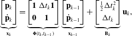 \begin{equation} \underbrace{\begin{bmatrix} \mathbf{p}_{k} \\[3pt] \dot{\mathbf{p}}_{k} \end{bmatrix}}_{\mathbf{x}_{k}} = \underbrace{\begin{bmatrix} \mathbf{1} & \Delta t_k \mathbf{1} \\[3pt] \mathbf{0} & \mathbf{1} \end{bmatrix}}_{{\boldsymbol{\Phi }}(t_k, t_{k-1})} \underbrace{\begin{bmatrix} \mathbf{p}_{k-1} \\[3pt] \dot{\mathbf{p}}_{k-1} \end{bmatrix}}_{\mathbf{x}_{k-1}} + \underbrace{\begin{bmatrix} \frac{1}{2}\Delta t_k^2 \\[3pt] \Delta t_k \end{bmatrix}}_{\mathbf{B}_k} \mathbf{u}_k, \end{equation}
where $\Delta t_k = t_k - t_{k-1}$
,
$\Delta t_k = t_k - t_{k-1}$
, ${\boldsymbol{\Phi }}(t_k, t_{k-1})$
is the transition function, and
${\boldsymbol{\Phi }}(t_k, t_{k-1})$
is the transition function, and $\mathbf{u}_k$
are acceleration measurements. A preintegration window is then defined between two endpoints,
$\mathbf{u}_k$
are acceleration measurements. A preintegration window is then defined between two endpoints, $(t_{k-1}, t_k)$
, which includes times
$(t_{k-1}, t_k)$
, which includes times $\tau _0, \ldots, \tau _J$
. Following the approach of [Reference Lupton and Sukkarieh1, Reference Forster, Carlone, Dellaert and Scaramuzza2], the preintegrated measurements
$\tau _0, \ldots, \tau _J$
. Following the approach of [Reference Lupton and Sukkarieh1, Reference Forster, Carlone, Dellaert and Scaramuzza2], the preintegrated measurements $\Delta \mathbf{x}_{k, k-1}$
are computed as:
$\Delta \mathbf{x}_{k, k-1}$
are computed as:
 \begin{equation} \Delta \mathbf{x}_{k,k-1} = \sum _{n=1}^{J}{\boldsymbol{\Phi }}(\tau _J, \tau _n) \mathbf{B}_n \mathbf{u}_n. \end{equation}
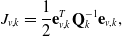
These preintegrated measurements can be used to replace the acceleration measurements with a single relative motion factor between two endpoints:
 \begin{align} J_{v,k} &= \frac{1}{2}\mathbf{e}_{k}^T \boldsymbol{\Sigma }_{k}^{-1} \mathbf{e}_{k}, \\[-2pt] \nonumber \end{align}
 \begin{align} \mathbf{e}_{k} &= \mathbf{x}_k -{\boldsymbol{\Phi }}(t_k, t_{k-1}) \mathbf{x}_{k-1} - \Delta \mathbf{x}_{k, k-1}, \end{align}
where
 \begin{equation} \boldsymbol{\Sigma }_k = \sum _{n=1}^J{\boldsymbol{\Phi }}(\tau _J, \tau _n) \mathbf{B}_n \mathbf{Q}_n \mathbf{B}_n^T{\boldsymbol{\Phi }}(\tau _J, \tau _n)^T, \end{equation}
and $\mathbf{Q}_n$
is the covariance of the acceleration input
$\mathbf{Q}_n$
is the covariance of the acceleration input $\mathbf{u}_n \sim \mathcal{N}(\mathbf{0}, \mathbf{Q}_n)$
. Note that in this approach, uncertainty is propagated using the covariance on the acceleration input,
$\mathbf{u}_n \sim \mathcal{N}(\mathbf{0}, \mathbf{Q}_n)$
. Note that in this approach, uncertainty is propagated using the covariance on the acceleration input, $\mathbf{Q}_n$
, which conflates IMU measurement noise and the underlying process noise. If the acceleration measurements were to drop out suddenly, it is unclear how the state and covariance should be propagated using this approach. It can be shown that preintegration is mathematically equivalent to marginalizing out the states between
$\mathbf{Q}_n$
, which conflates IMU measurement noise and the underlying process noise. If the acceleration measurements were to drop out suddenly, it is unclear how the state and covariance should be propagated using this approach. It can be shown that preintegration is mathematically equivalent to marginalizing out the states between $\mathbf{x}_{k-1}$
and
$\mathbf{x}_{k-1}$
and $\mathbf{x}_k$
. The overall objective function that we seek to minimize is then
$\mathbf{x}_k$
. The overall objective function that we seek to minimize is then
 \begin{equation} J(\mathbf{x}) = \sum _{k=0}^K \left (J_{v,k}(\mathbf{x}) + J_{y,k}(\mathbf{x}) \right ), \end{equation}
where
 \begin{equation} J_{y,k} = \frac{1}{2} \left ( \mathbf{y}_k - \mathbf{C}_k \mathbf{x}_k\right )^T \mathbf{R}_k^{-1} \left ( \mathbf{y}_k - \mathbf{C}_k \mathbf{x}_k \right ) \end{equation}
are the measurement factors, and $\mathbf{R}_k$
is the associated measurement covariance.
$\mathbf{R}_k$
is the associated measurement covariance.
3.2. Continuous-time state estimation
In order to incorporate potentially asynchronous position and acceleration measurements, we propose to carry out continuous-time trajectory estimation as exactly sparse Gaussian process regression [Reference Anderson, Barfoot, Tong and Särkkä27–Reference Barfoot29]. We consider systems with a Gaussian process (GP) prior and a linear measurement model:
 \begin{align} \mathbf{x}(t) &\sim \mathcal{GP}(\check{\mathbf{x}}(t), \check{\mathbf{P}}(t, t^\prime )), \\[-2pt] \nonumber \end{align}
 \begin{align} \mathbf{y}_k &= \mathbf{C}_k \mathbf{x}(t_k) + \mathbf{n}_k,\\[12pt] \nonumber \end{align}
where $\mathbf{x}(t)$
is the state,
$\mathbf{x}(t)$
is the state, $\check{\mathbf{x}}(t)$
is the mean function,
$\check{\mathbf{x}}(t)$
is the mean function, $\check{\mathbf{P}}(t, t^\prime )$
is the covariance function, and
$\check{\mathbf{P}}(t, t^\prime )$
is the covariance function, and $\mathbf{y}_k$
are measurements corrupted by zero-mean Gaussian noise
$\mathbf{y}_k$
are measurements corrupted by zero-mean Gaussian noise $\mathbf{n}_k \sim \mathcal{N}(\mathbf{0}, \mathbf{R}_k)$
. In this section, we restrict our attention to a class of GP priors resulting from linear time-invariant (LTI) stochastic differential equations (SDEs) of the form:
$\mathbf{n}_k \sim \mathcal{N}(\mathbf{0}, \mathbf{R}_k)$
. In this section, we restrict our attention to a class of GP priors resulting from linear time-invariant (LTI) stochastic differential equations (SDEs) of the form:
 \begin{align} \dot{\mathbf{x}}(t) &= \boldsymbol{A} \mathbf{x}(t) + \boldsymbol{B} \mathbf{u}(t) + \boldsymbol{L} \mathbf{w}(t), \\[3pt] \mathbf{w}(t) &\sim \mathcal{GP}(\mathbf{0}, \boldsymbol{Q} \delta (t - t^\prime )), \nonumber \end{align}
where $\mathbf{w}(t)$
is a white-noise Gaussian process,
$\mathbf{w}(t)$
is a white-noise Gaussian process, $\boldsymbol{Q}$
is a power spectral density matrix, and
$\boldsymbol{Q}$
is a power spectral density matrix, and $\mathbf{u}(t)$
is a known exogenous input. The general solution to this differential equation is
$\mathbf{u}(t)$
is a known exogenous input. The general solution to this differential equation is
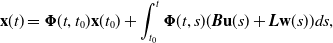 \begin{equation} \mathbf{x}(t) ={\boldsymbol{\Phi }}(t, t_0) \mathbf{x}(t_0) + \int _{t_0}^t{\boldsymbol{\Phi }}(t, s) (\boldsymbol{B} \mathbf{u}(s) + \boldsymbol{L} \mathbf{w}(s)) ds, \end{equation}
where ${\boldsymbol{\Phi }}(t, s) = \exp\! (\mathbf{A}(t - s))$
is the transition function. The mean function is
${\boldsymbol{\Phi }}(t, s) = \exp\! (\mathbf{A}(t - s))$
is the transition function. The mean function is
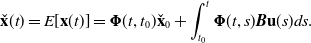 \begin{equation} \check{\mathbf{x}}(t) = E[\mathbf{x}(t)] ={\boldsymbol{\Phi }}(t, t_0) \check{\mathbf{x}}_0 + \int _{t_0}^t{\boldsymbol{\Phi }}(t, s) \boldsymbol{B} \mathbf{u}(s) ds. \end{equation}
Over a sequence of estimation times, $t_0 \lt t_1 \lt \cdots \lt t_K$
, the mean function can be written as:
$t_0 \lt t_1 \lt \cdots \lt t_K$
, the mean function can be written as:
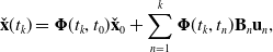 \begin{equation} \check{\mathbf{x}}(t_k) ={\boldsymbol{\Phi }}(t_k, t_0) \check{\mathbf{x}}_0 + \sum _{n=1}^k{\boldsymbol{\Phi }}(t_k, t_n) \mathbf{B}_n \mathbf{u}_n, \end{equation}
assuming piecewise-constant input $\mathbf{u}_n$
. This can be rewritten in a lifted form as:
$\mathbf{u}_n$
. This can be rewritten in a lifted form as:
 \begin{equation} \check{\mathbf{x}} = \mathbf{A} \mathbf{B} \mathbf{u}, \end{equation}
where $\mathbf{A}$
is the lifted lower-triangular transition matrix, the inverse of which is
$\mathbf{A}$
is the lifted lower-triangular transition matrix, the inverse of which is
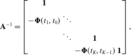 \begin{equation} \mathbf{A}^{-1} = \begin{bmatrix} \mathbf{1} \\[3pt] -{\boldsymbol{\Phi }}(t_1,t_0) & \ddots \\[3pt] & \ddots & \mathbf{1} \\[3pt] & & -{\boldsymbol{\Phi }}(t_K,t_{K-1}) & \mathbf{1} \end{bmatrix}, \end{equation} $\mathbf{B} = \textrm{diag}(\mathbf{1}, \boldsymbol{B}_1, \cdots, \boldsymbol{B}_K)$
, and
$\mathbf{B} = \textrm{diag}(\mathbf{1}, \boldsymbol{B}_1, \cdots, \boldsymbol{B}_K)$
, and $\mathbf{u} = [\check{\mathbf{x}}_0^T\,\mathbf{u}_1^T\,\cdots \,\mathbf{u}_K^T]^T$
. See [Reference Barfoot29] for further details on the formulations above. The covariance function is then
$\mathbf{u} = [\check{\mathbf{x}}_0^T\,\mathbf{u}_1^T\,\cdots \,\mathbf{u}_K^T]^T$
. See [Reference Barfoot29] for further details on the formulations above. The covariance function is then
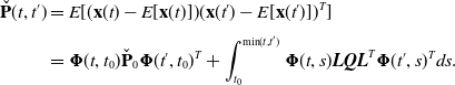 \begin{align} \check{\mathbf{P}}(t, t^\prime ) & = E[(\mathbf{x}(t) - E[\mathbf{x}(t)]) (\mathbf{x}(t^\prime ) - E[\mathbf{x}(t^\prime )])^T]\\[3pt] &={\boldsymbol{\Phi }}(t, t_0) \check{\mathbf{P}}_0{\boldsymbol{\Phi }}(t^\prime, t_0)^T + \int _{t_0}^{\textrm{min}(t, t^\prime )}{\boldsymbol{\Phi }}(t, s) \boldsymbol{L} \boldsymbol{Q} \boldsymbol{L}^T{\boldsymbol{\Phi }}(t^\prime, s)^T ds \nonumber . \end{align}
The covariance can also be rewritten in a lifted form using the same set of estimation times as above:
 \begin{equation} \check{\mathbf{P}} = \mathbf{A}\mathbf{Q}\mathbf{A}^T, \end{equation}
where $\mathbf{Q} = \textrm{diag}(\check{\mathbf{P}}_0, \mathbf{Q}_1, \cdots, \mathbf{Q}_K)$
, and
$\mathbf{Q} = \textrm{diag}(\check{\mathbf{P}}_0, \mathbf{Q}_1, \cdots, \mathbf{Q}_K)$
, and
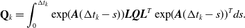 \begin{equation} \mathbf{Q}_k = \int _0^{\Delta t_k} \exp\! (\boldsymbol{A}(\Delta t_k - s)) \boldsymbol{L} \boldsymbol{Q} \boldsymbol{L}^T \exp\! (\boldsymbol{A}(\Delta t_k - s))^T ds. \end{equation}
Our prior over the entire trajectory can then be written as:
 \begin{equation} \mathbf{x} \sim \mathcal{N}(\check{\mathbf{x}}, \check{\mathbf{P}}), \end{equation}
where $\check{\mathbf{P}}$
is the kernel matrix. Note that the inverse kernel matrix
$\check{\mathbf{P}}$
is the kernel matrix. Note that the inverse kernel matrix $\check{\mathbf{P}}^{-1}$
is block-tridiagonal thanks to the Markovian nature of the state. This sparsity property also holds for linear time-varying (LTV) SDEs, provided that they are also Markovian [Reference Anderson and Barfoot28]. The exact sparsity of
$\check{\mathbf{P}}^{-1}$
is block-tridiagonal thanks to the Markovian nature of the state. This sparsity property also holds for linear time-varying (LTV) SDEs, provided that they are also Markovian [Reference Anderson and Barfoot28]. The exact sparsity of $\check{\mathbf{P}}^{-1}$
is what allows us to perform efficient Gaussian process regression. This fact can be observed more easily by inspecting the following linear system of equations:
$\check{\mathbf{P}}^{-1}$
is what allows us to perform efficient Gaussian process regression. This fact can be observed more easily by inspecting the following linear system of equations:
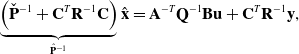 \begin{equation} \underbrace{\left ( \check{\mathbf{P}}^{-1} + \mathbf{C}^T \mathbf{R}^{-1} \mathbf{C} \right )}_{\hat{\mathbf{P}}^{-1}} \hat{\mathbf{x}} = \mathbf{A}^{-T} \mathbf{Q}^{-1} \mathbf{B} \mathbf{u} + \mathbf{C}^T \mathbf{R}^{-1} \mathbf{y}, \end{equation}
where the Hessian is on the left-hand side, $\hat{\mathbf{P}}^{-1}$
is block-tridiagonal since
$\hat{\mathbf{P}}^{-1}$
is block-tridiagonal since $\check{\mathbf{P}}^{-1}$
is block-tridiagonal, and
$\check{\mathbf{P}}^{-1}$
is block-tridiagonal, and $\mathbf{C}^T \mathbf{R}^{-1} \mathbf{C}$
is block-diagonal. Thus, this linear system of equations can be solved in
$\mathbf{C}^T \mathbf{R}^{-1} \mathbf{C}$
is block-diagonal. Thus, this linear system of equations can be solved in $O(K)$
time using a sparse Cholesky solver. The exact sparsity of
$O(K)$
time using a sparse Cholesky solver. The exact sparsity of $\check{\mathbf{P}}^{-1}$
also enables us to perform efficient Gaussian process interpolation. The standard GP interpolation formulas are given by:
$\check{\mathbf{P}}^{-1}$
also enables us to perform efficient Gaussian process interpolation. The standard GP interpolation formulas are given by:
 \begin{align} \hat{\mathbf{x}}(\tau ) &= \check{\mathbf{x}}(\tau ) + \check{\mathbf{P}}(\tau )\check{\mathbf{P}}^{-1} (\hat{\mathbf{x}} - \check{\mathbf{x}}), \\[-2pt] \nonumber \end{align}
 \begin{align} \hat{\mathbf{P}}(\tau, \tau ) &= \check{\mathbf{P}}(\tau, \tau ) + \check{\mathbf{P}}(\tau )\check{\mathbf{P}}^{-1}\left (\hat{\mathbf{P}} - \check{\mathbf{P}} \right ) \check{\mathbf{P}}^{-T} \check{\mathbf{P}}(\tau )^T, \\[12pt] \nonumber \end{align}
where
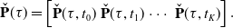 \begin{equation} \check{\mathbf{P}}(\tau ) = \begin{bmatrix} \check{\mathbf{P}}(\tau, t_0) & \check{\mathbf{P}}(\tau, t_1) & \cdots & \check{\mathbf{P}}(\tau, t_K) \end{bmatrix}. \end{equation}
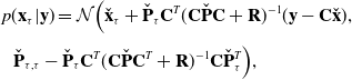
The key to performing efficient interpolation relies on the sparsity of
 \begin{equation} \check{\mathbf{P}}(\tau )\check{\mathbf{P}}^{-1} = \begin{bmatrix} \mathbf{0} & \cdots & \mathbf{0} & \boldsymbol{\Lambda }(\tau ) & \boldsymbol{\Psi }(\tau ) & \mathbf{0} & \cdots & \mathbf{0} \end{bmatrix}, \end{equation}
where
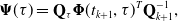 \begin{align} \boldsymbol{\Psi }(\tau ) &= \mathbf{Q}_\tau \boldsymbol{\Phi }(t_{k+1}, \tau )^T \mathbf{Q}_{k+1}^{-1}, \\[-2pt] \nonumber \end{align}
 \begin{align} \boldsymbol{\Lambda }(\tau ) &= \boldsymbol{\Phi }(\tau, t_k) - \boldsymbol{\Psi }(\tau ) \boldsymbol{\Phi }(t_{k+1}, t_k), \\[12pt] \nonumber \end{align}
are the only nonzero block columns at indices $k+1$
and
$k+1$
and $k$
, respectively. Thus, each interpolation query of the posterior trajectory is an
$k$
, respectively. Thus, each interpolation query of the posterior trajectory is an $O(1)$
operation.
$O(1)$
operation.
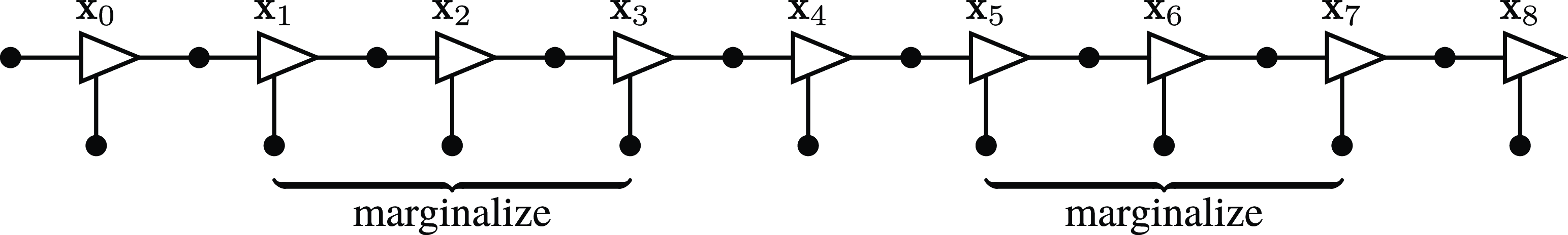
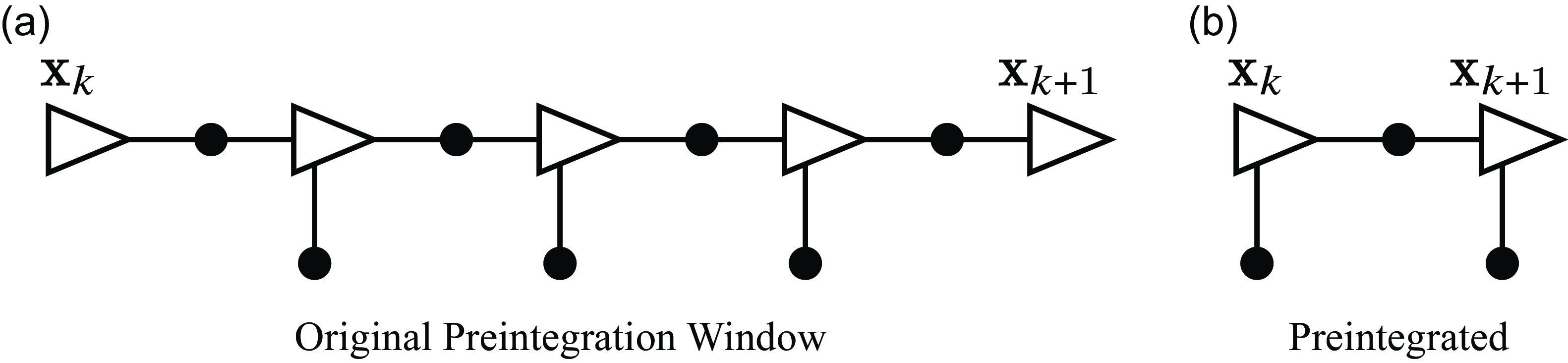
In this factor graph, we consider a case where we would like to marginalize several states out of the full Bayesian posterior. The triangles represent states and the black dots represent factors. This factor graph could potentially correspond to doing continuous-time state estimation with binary motion prior factors, unary measurement factors, and a unary prior factor on the initial state $\mathbf{x}_0$
.
$\mathbf{x}_0$
.
3.3. A generalization to preintegration
In Section 3.1, we showed how to perform preintegration when considering acceleration measurements as inputs to a motion model following closely from [Reference Lupton and Sukkarieh1, Reference Forster, Carlone, Dellaert and Scaramuzza2]. In this section, we generalize the concept of preintegration to support heterogeneous factors (a combination of binary factors and unary factors). An example factor graph is shown in Figure 1. As a motivating example, consider having measurements of position such as from a GPS and measurements of acceleration coming from an accelerometer. These are unary measurement factors, called such because they only involve a single state. The binary factors here are motion prior factors derived from our Gaussian process motion prior, called binary because they are between two states. In classic preintegration, the only factors that are preintegrated are binary factors. Here, we show that we can simply use the formulas for querying a Gaussian process posterior at the endpoints of the preintegration window to form a preintegration factor that summarizes all the measurements contained therein. First, we consider the joint density of the state at a set of query times $(\tau _0 \lt \tau _1 \lt \cdots \lt \tau _J)$
and the measurements:
$(\tau _0 \lt \tau _1 \lt \cdots \lt \tau _J)$
and the measurements:
 \begin{equation} p\left (\begin{bmatrix} \mathbf{x}_\tau \\[3pt] \mathbf{y} \end{bmatrix} \right ) = \mathcal{N} \left ( \begin{bmatrix} \check{\mathbf{x}}_\tau \\[3pt] \mathbf{C} \check{\mathbf{x}}_\tau \end{bmatrix}, \begin{bmatrix} \check{\mathbf{P}}_{\tau, \tau } & \check{\mathbf{P}}_\tau \mathbf{C}^T \\[3pt] \mathbf{C} \check{\mathbf{P}}_\tau ^T & \mathbf{R} + \mathbf{C} \check{\mathbf{P}} \mathbf{C}^T \end{bmatrix}\right ). \end{equation}
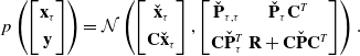
We then perform the usual factoring using a Schur complement to obtain the posterior:
 \begin{align} &p(\mathbf{x}_\tau | \mathbf{y}) = \mathcal{N} \Big ( \check{\mathbf{x}}_\tau + \check{\mathbf{P}}_\tau \mathbf{C}^T (\mathbf{C} \check{\mathbf{P}} \mathbf{C} + \mathbf{R})^{-1} (\mathbf{y} - \mathbf{C} \check{\mathbf{x}}), \nonumber \\[3pt] &\,\,\,\check{\mathbf{P}}_{\tau, \tau } - \check{\mathbf{P}}_\tau \mathbf{C}^T(\mathbf{C} \check{\mathbf{P}} \mathbf{C}^T + \mathbf{R})^{-1} \mathbf{C} \check{\mathbf{P}}_\tau ^T \Big ), \end{align}
where we obtain expressions for $\hat{\mathbf{x}}_\tau$
and
$\hat{\mathbf{x}}_\tau$
and $\hat{\mathbf{P}}_{\tau, \tau }$
. We rearrange this further by inserting
$\hat{\mathbf{P}}_{\tau, \tau }$
. We rearrange this further by inserting $\check{\mathbf{P}}^{-1}\check{\mathbf{P}}$
after the first instance of
$\check{\mathbf{P}}^{-1}\check{\mathbf{P}}$
after the first instance of $\check{\mathbf{P}}_\tau$
and by applying the Sherman–Morrison–Woodbury identities to obtain
$\check{\mathbf{P}}_\tau$
and by applying the Sherman–Morrison–Woodbury identities to obtain
 \begin{align} &\hat{\mathbf{x}}_\tau = \check{\mathbf{x}}_\tau + \check{\mathbf{P}}_\tau \check{\mathbf{P}}^{-1} (\check{\mathbf{P}}^{-1} + \mathbf{C}^T\mathbf{R}^{-1}\mathbf{C})^{-1} \mathbf{C}^T \mathbf{R}^{-1} (\mathbf{y} - \mathbf{C} \check{\mathbf{x}}), \\[-2pt] \nonumber \end{align}
 \begin{align} &\hat{\mathbf{P}}_{\tau, \tau } = \check{\mathbf{P}}_{\tau, \tau } - \check{\mathbf{P}}_\tau \check{\mathbf{P}}^{-1} (\check{\mathbf{P}}^{-1} + \mathbf{C}^T\mathbf{R}^{-1}\mathbf{C})^{-1} \mathbf{C}^T \mathbf{R}^{-1} \mathbf{C} \check{\mathbf{P}}_\tau ^T, \\[12pt] \nonumber \end{align}
where we note that $(\check{\mathbf{P}}^{-1} + \mathbf{C}^T\mathbf{R}^{-1}\mathbf{C})$
is block-tridiagonal, and so the product
$(\check{\mathbf{P}}^{-1} + \mathbf{C}^T\mathbf{R}^{-1}\mathbf{C})$
is block-tridiagonal, and so the product $(\check{\mathbf{P}}^{-1} + \mathbf{C}^T\mathbf{R}^{-1}\mathbf{C})^{-1} \mathbf{C}^T \mathbf{R}^{-1} (\mathbf{y} - \mathbf{C} \check{\mathbf{x}})$
can be evaluated in
$(\check{\mathbf{P}}^{-1} + \mathbf{C}^T\mathbf{R}^{-1}\mathbf{C})^{-1} \mathbf{C}^T \mathbf{R}^{-1} (\mathbf{y} - \mathbf{C} \check{\mathbf{x}})$
can be evaluated in $O(K)$
time using a sparse Cholesky solver. When we encounter products resembling
$O(K)$
time using a sparse Cholesky solver. When we encounter products resembling $\mathbf{A}^{-1}\mathbf{b}$
where
$\mathbf{A}^{-1}\mathbf{b}$
where $\mathbf{A}$
is block-tridiagonal, we can instead solve
$\mathbf{A}$
is block-tridiagonal, we can instead solve $\mathbf{A}\mathbf{z} = \mathbf{b}$
for
$\mathbf{A}\mathbf{z} = \mathbf{b}$
for $\mathbf{z}$
using an efficient solver that takes advantage of the sparsity of
$\mathbf{z}$
using an efficient solver that takes advantage of the sparsity of $\mathbf{A}$
. Finally, the product
$\mathbf{A}$
. Finally, the product $\check{\mathbf{P}}_\tau \check{\mathbf{P}}^{-1}$
is quite sparse, having only two nonzero block columns per block row as shown earlier in (21). It follows that
$\check{\mathbf{P}}_\tau \check{\mathbf{P}}^{-1}$
is quite sparse, having only two nonzero block columns per block row as shown earlier in (21). It follows that $\hat{\mathbf{x}}_\tau$
and
$\hat{\mathbf{x}}_\tau$
and $\hat{\mathbf{P}}_{\tau, \tau }$
can be computed in time that scales linearly with the number of measurements. Now, we consider the case where the query times consist of the beginning and end of a preintegration window,
$\hat{\mathbf{P}}_{\tau, \tau }$
can be computed in time that scales linearly with the number of measurements. Now, we consider the case where the query times consist of the beginning and end of a preintegration window, $(t_k, t_{k+1})$
. The queried mean and covariance can be treated as pseudomeasurements summarizing the measurements contained in the preintegration window. We adjust our notation to make it clear that these are now being treated as measurements by using
$(t_k, t_{k+1})$
. The queried mean and covariance can be treated as pseudomeasurements summarizing the measurements contained in the preintegration window. We adjust our notation to make it clear that these are now being treated as measurements by using $\tilde{\mathbf{x}}$
instead of
$\tilde{\mathbf{x}}$
instead of $\hat{\mathbf{x}}$
. What we obtain is a joint Gaussian factor for the states at times
$\hat{\mathbf{x}}$
. What we obtain is a joint Gaussian factor for the states at times $t_k$
and
$t_k$
and $t_{k+1}$
:
$t_{k+1}$
:
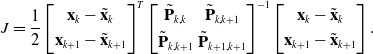 \begin{align} J = \frac{1}{2} &\begin{bmatrix} \mathbf{x}_k - \tilde{\mathbf{x}}_k \\[3pt] \mathbf{x}_{k+1} - \tilde{\mathbf{x}}_{k+1} \end{bmatrix}^T \begin{bmatrix} \tilde{\mathbf{P}}_{k,k} & \tilde{\mathbf{P}}_{k,k+1}\\[3pt]{\tilde{\mathbf{P}}_{k,k+1}} & \tilde{\mathbf{P}}_{k+1,k+1} \end{bmatrix}^{-1} \begin{bmatrix} \mathbf{x}_k - \tilde{\mathbf{x}}_k \\[3pt] \mathbf{x}_{k+1} - \tilde{\mathbf{x}}_{k+1} \end{bmatrix}. \end{align}
This figure depicts the results of our preintegration, which can incorporate heterogeneous factors. The resulting joint Gaussian factor in (26) can be thought of as two unary factors, one each for $\mathbf{x}_k$
and
$\mathbf{x}_k$
and $\mathbf{x}_{k+1}$
, and an additional binary factor between
$\mathbf{x}_{k+1}$
, and an additional binary factor between $\mathbf{x}_k$
and
$\mathbf{x}_k$
and $\mathbf{x}_{k+1}$
.
$\mathbf{x}_{k+1}$
.
A diagram depicting how this affects the resulting factor graph is shown in Figure 2. Using this approach, we can ‘preintegrate’ heterogeneous factors between pairs of states. One clear advantage of this approach is that it offers a tidy method for bookkeeping measurement costs and uncertainties. In the supplementary materials, we provide an alternative formulation using a Schur complement with the same linear time complexity. Indeed, marginalization with a Schur complement is equivalent to the presented marginalization approach using a Gaussian process. However, the Gaussian process still serves a useful purpose in creating motion prior factors. Furthermore, the Gaussian process provides methods for interpolating the posterior.
It is unclear how to extend this marginalization approach to $SE(3)$
due to our choice to approximate
$SE(3)$
due to our choice to approximate $SE(3)$
trajectories using sequences of local Gaussian processes [Reference Anderson and Barfoot28]. It is possible that this marginalization approach could be applied using a global GP formulation such as the one presented by Le Gentil and Vidal-Calleja [Reference Gentil and Vidal-Calleja17]. However, their approach must contend with rotational singularities. We leave the extension to
$SE(3)$
trajectories using sequences of local Gaussian processes [Reference Anderson and Barfoot28]. It is possible that this marginalization approach could be applied using a global GP formulation such as the one presented by Le Gentil and Vidal-Calleja [Reference Gentil and Vidal-Calleja17]. However, their approach must contend with rotational singularities. We leave the extension to $SE(3)$
as an area of future work. In our implementation of lidar-inertial odometry, we instead use the posterior Gaussian process interpolation formula as in (19) to form continuous-time measurement factors. This is actually an approximation, as it is not exactly the same as marginalization. However, we have found the interpolation approach to work well in practice. Furthermore, the interpolation approach lends itself quite easily to parallelization enabling a highly efficient implementation.
$SE(3)$
as an area of future work. In our implementation of lidar-inertial odometry, we instead use the posterior Gaussian process interpolation formula as in (19) to form continuous-time measurement factors. This is actually an approximation, as it is not exactly the same as marginalization. However, we have found the interpolation approach to work well in practice. Furthermore, the interpolation approach lends itself quite easily to parallelization enabling a highly efficient implementation.
3.4. IMU as a measurement
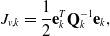
In our proposed approach, we treat IMU measurements as direct measurements of the state within a continuous-time estimation framework. For the 1D toy problem, we chose to use a Singer prior, which is defined by the following LTI SDE:
 \begin{align} \dddot{\mathbf{p}}(t) &= -\boldsymbol{\alpha } \ddot{\mathbf{p}}(t) + \mathbf{w}(t), \\[3pt] \mathbf{w}(t) &\sim \mathcal{GP}(\mathbf{0}, \mathbf{Q}_c \delta (t - t^\prime )), \nonumber \end{align}
where $\mathbf{w}(t)$
is a white-noise Gaussian process and
$\mathbf{w}(t)$
is a white-noise Gaussian process and $\mathbf{Q}_c\,=\,2 \boldsymbol{\alpha } \boldsymbol{\sigma }^2$
is the power spectral density matrix [Reference Wong, Yoon, Schoellig and Barfoot30]. By varying
$\mathbf{Q}_c\,=\,2 \boldsymbol{\alpha } \boldsymbol{\sigma }^2$
is the power spectral density matrix [Reference Wong, Yoon, Schoellig and Barfoot30]. By varying $\boldsymbol{\alpha }$
and
$\boldsymbol{\alpha }$
and $\boldsymbol{\sigma }^2$
, the Singer prior can model motion priors ranging from WNOA (
$\boldsymbol{\sigma }^2$
, the Singer prior can model motion priors ranging from WNOA ( $\boldsymbol{\alpha } \rightarrow \boldsymbol{\infty }, \tilde{\boldsymbol{\sigma }}^2 = \boldsymbol{\alpha }^2 \boldsymbol{\sigma }^2$
) to WNOJ (
$\boldsymbol{\alpha } \rightarrow \boldsymbol{\infty }, \tilde{\boldsymbol{\sigma }}^2 = \boldsymbol{\alpha }^2 \boldsymbol{\sigma }^2$
) to WNOJ ( $\boldsymbol{\alpha }{\rightarrow } \mathbf{0}$
). The discrete-time motion model is given by:
$\boldsymbol{\alpha }{\rightarrow } \mathbf{0}$
). The discrete-time motion model is given by:
 \begin{align} &\mathbf{x}_{k} ={\boldsymbol{\Phi }}(t_{k},t_{k-1}) \mathbf{x}_{k-1} + \mathbf{w}_k, \quad \mathbf{w}_k \sim \mathcal{N}(\mathbf{0}, \mathbf{Q}_k), \end{align}
where $\mathbf{w}_k$
is the process noise,
$\mathbf{w}_k$
is the process noise, $\mathbf{x}_k = [\mathbf{p}_{k}^T\,\dot{\mathbf{p}}_{k}^T\,\ddot{\mathbf{p}}_{k}^T]^T$
,
$\mathbf{x}_k = [\mathbf{p}_{k}^T\,\dot{\mathbf{p}}_{k}^T\,\ddot{\mathbf{p}}_{k}^T]^T$
, ${\boldsymbol{\Phi }}(t_{k},t_{k-1})$
is the state transition function, and
${\boldsymbol{\Phi }}(t_{k},t_{k-1})$
is the state transition function, and $\mathbf{Q}_k$
is the discrete-time covariance. Expressions for
$\mathbf{Q}_k$
is the discrete-time covariance. Expressions for ${\boldsymbol{\Phi }}(t_{k},t_{k-1})$
and
${\boldsymbol{\Phi }}(t_{k},t_{k-1})$
and $\mathbf{Q}_k$
for the Singer prior are provided by Wong et al. [Reference Wong, Yoon, Schoellig and Barfoot30] and are repeated in the supplementary materials. The binary motion prior factors are given by:
$\mathbf{Q}_k$
for the Singer prior are provided by Wong et al. [Reference Wong, Yoon, Schoellig and Barfoot30] and are repeated in the supplementary materials. The binary motion prior factors are given by:
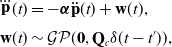
 \begin{align} J_{v,k} &= \frac{1}{2}\mathbf{e}_{k}^T \mathbf{Q}_{k}^{-1} \mathbf{e}_{k}, \\[-12pt] \nonumber \end{align}
 \begin{align} \mathbf{e}_k &= \mathbf{x}_k -{\boldsymbol{\Phi }}(t_k, t_{k-1}) \mathbf{x}_{k-1}. \\[12pt] \nonumber \end{align}
The unary measurement factors have the same form as in (6) except that now accelerations are treated as direct measurements of the state. In addition, the overall objective is the same as in (5). We arrive at the linear system of equations from (18). By default, this approach would require that we estimate the state at each measurement time. In order to reduce the size of the state space, as in Section 3.1, we build preintegrated factors using the approach presented in Section 3.3 in order to bundle together both the unary measurement factors as well as the binary motion prior factors into a single factor. In the exact same fashion as the IMU-as-input approach, we preintegrate between pairs of states associated with the low-rate measurement times.
3.5. Simulation results
In this section, we compare two different approaches to combining high-rate acceleration measurements with low-rate position measurements. We refer to these two different approaches as IMU-as-input and IMU-as-measurement. The comparison is conducted on a toy 1D simulation problem. We sample trajectories from a GP motion prior as defined in (17) by using standard methods for sampling from a multidimensional Gaussian [Reference Barfoot29].
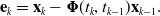
In our first simulation, we sample trajectories from a WNOJ motion prior with $Q_c = 1.0$
. Figure 3 provides a qualitative comparison of the IMU-as-input and IMU-as-measurement approaches for a single sampled simulation trajectory. Note that the performance of the two estimators including their 3-
$Q_c = 1.0$
. Figure 3 provides a qualitative comparison of the IMU-as-input and IMU-as-measurement approaches for a single sampled simulation trajectory. Note that the performance of the two estimators including their 3- $\sigma$
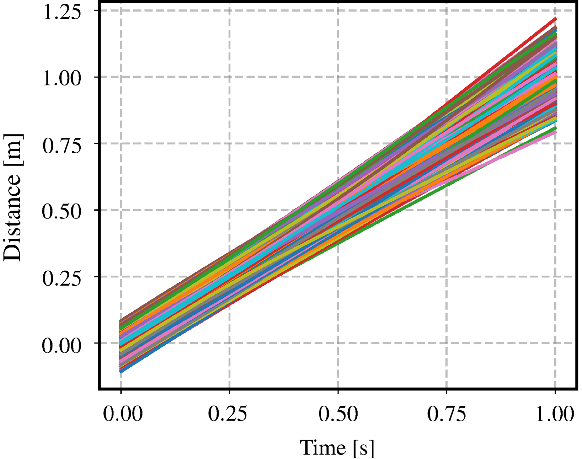
confidence bounds appears to be nearly identical. Figure 4 depicts 1000 trajectories sampled from this motion prior. In order to simulate noisy sensors, we also corrupt both position and acceleration measurements using zero-mean Gaussian noise where
$\sigma$
confidence bounds appears to be nearly identical. Figure 4 depicts 1000 trajectories sampled from this motion prior. In order to simulate noisy sensors, we also corrupt both position and acceleration measurements using zero-mean Gaussian noise where $y_{\textrm{pos},k} = \begin{bmatrix} 1 & 0 & 0 \end{bmatrix} \mathbf{x}_k + n_{\textrm{pos},k}$
,
$y_{\textrm{pos},k} = \begin{bmatrix} 1 & 0 & 0 \end{bmatrix} \mathbf{x}_k + n_{\textrm{pos},k}$
, $n_{\textrm{pos},k} \sim \mathcal{N}(0, \sigma ^2_{\textrm{pos}})$
,
$n_{\textrm{pos},k} \sim \mathcal{N}(0, \sigma ^2_{\textrm{pos}})$
, $y_{\textrm{acc},k} = \begin{bmatrix} 0 & 0 & 1 \end{bmatrix} \mathbf{x}_k + n_{\textrm{acc},k}$
, and
$y_{\textrm{acc},k} = \begin{bmatrix} 0 & 0 & 1 \end{bmatrix} \mathbf{x}_k + n_{\textrm{acc},k}$
, and $n_{\textrm{acc},k} \sim \mathcal{N}(0, \sigma ^2_{\textrm{acc}})$
. In the simulation, we set
$n_{\textrm{acc},k} \sim \mathcal{N}(0, \sigma ^2_{\textrm{acc}})$
. In the simulation, we set $\sigma _{\textrm{pos}} = 0.01m$
and
$\sigma _{\textrm{pos}} = 0.01m$
and $\sigma _{\textrm{acc}} = 0.01m/s^2$
.
$\sigma _{\textrm{acc}} = 0.01m/s^2$
.
The estimated trajectories of IMU-as-input and IMU-as-measurement are plotted alongside the ground-truth trajectory, which is sampled from white-noise-on-jerk motion prior with $Q_c = 1.0$
. Both methods were pretrained on a hold-out validation set of simulated trajectories.
$Q_c = 1.0$
. Both methods were pretrained on a hold-out validation set of simulated trajectories.
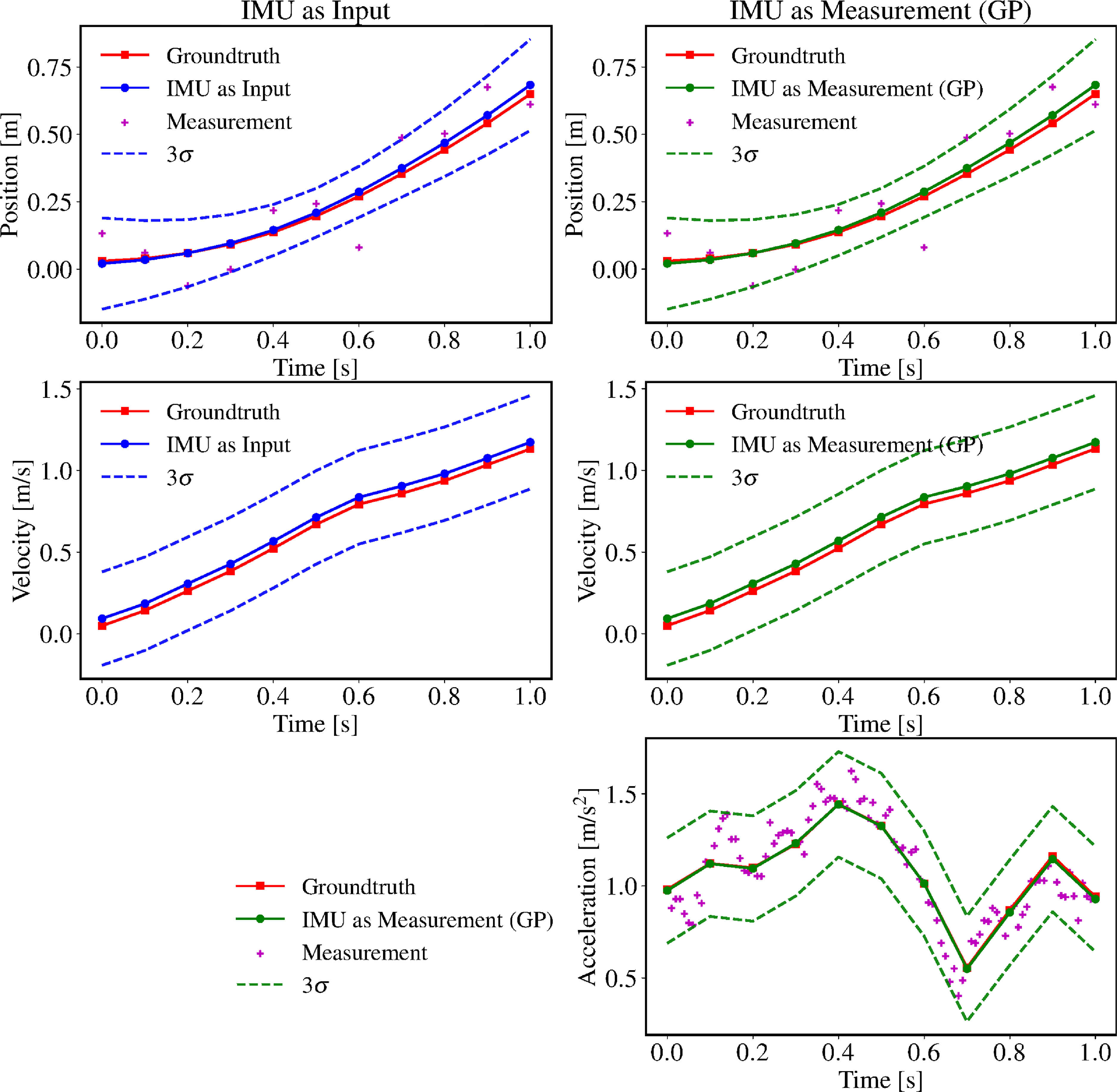
This figure depicts 1000 simulated trajectories sampled from a white-noise-on-jerk (WNOJ) prior where $\check{\mathbf{x}}_{0} = [0.0\,0.0\,1.0]^T$
,
$\check{\mathbf{x}}_{0} = [0.0\,0.0\,1.0]^T$
, $\check{\mathbf{P}}_{0} = \textrm{diag}(0.001, 0.001, 0.001)$
,
$\check{\mathbf{P}}_{0} = \textrm{diag}(0.001, 0.001, 0.001)$
, $Q_c = 1.0$
.
$Q_c = 1.0$
.
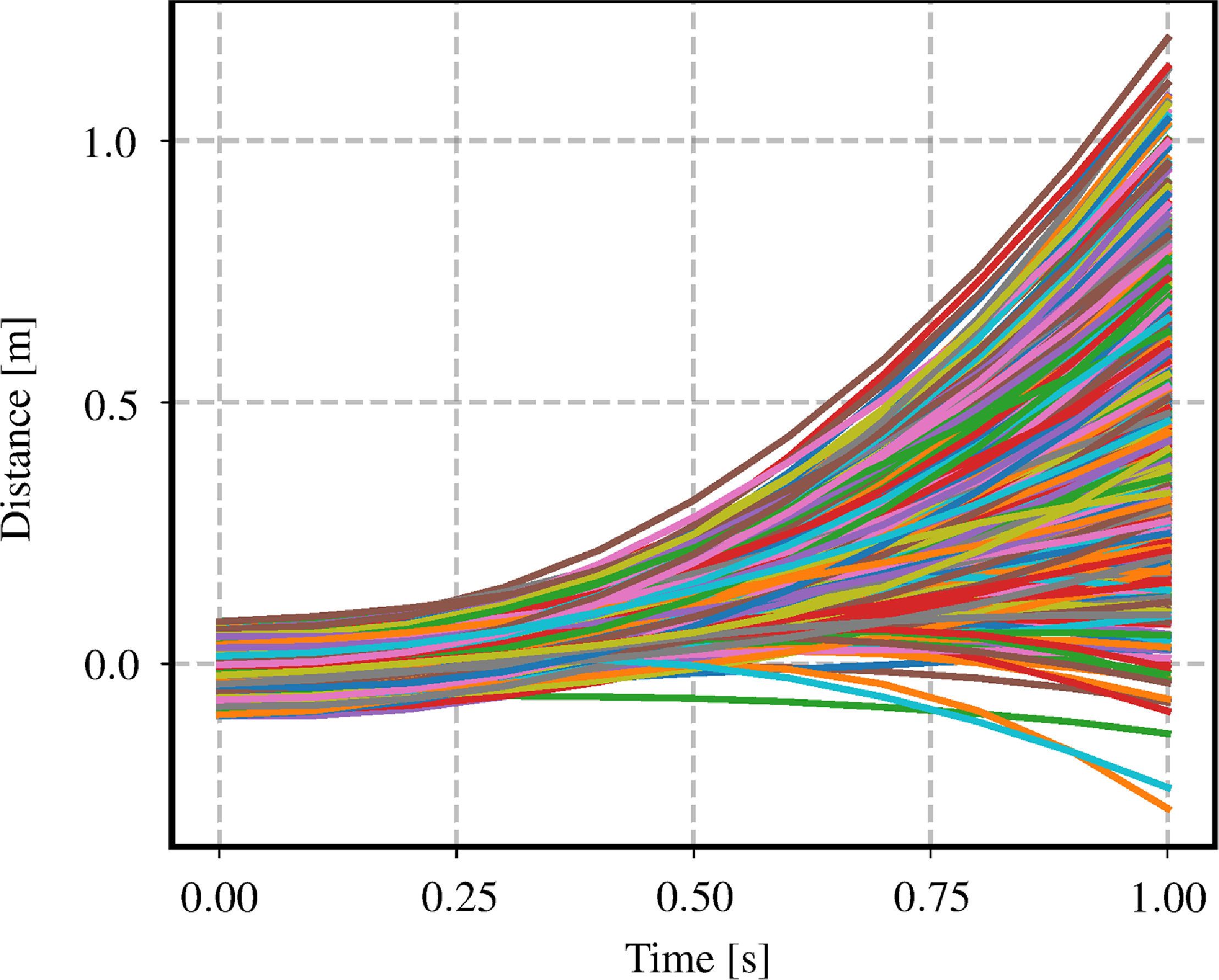
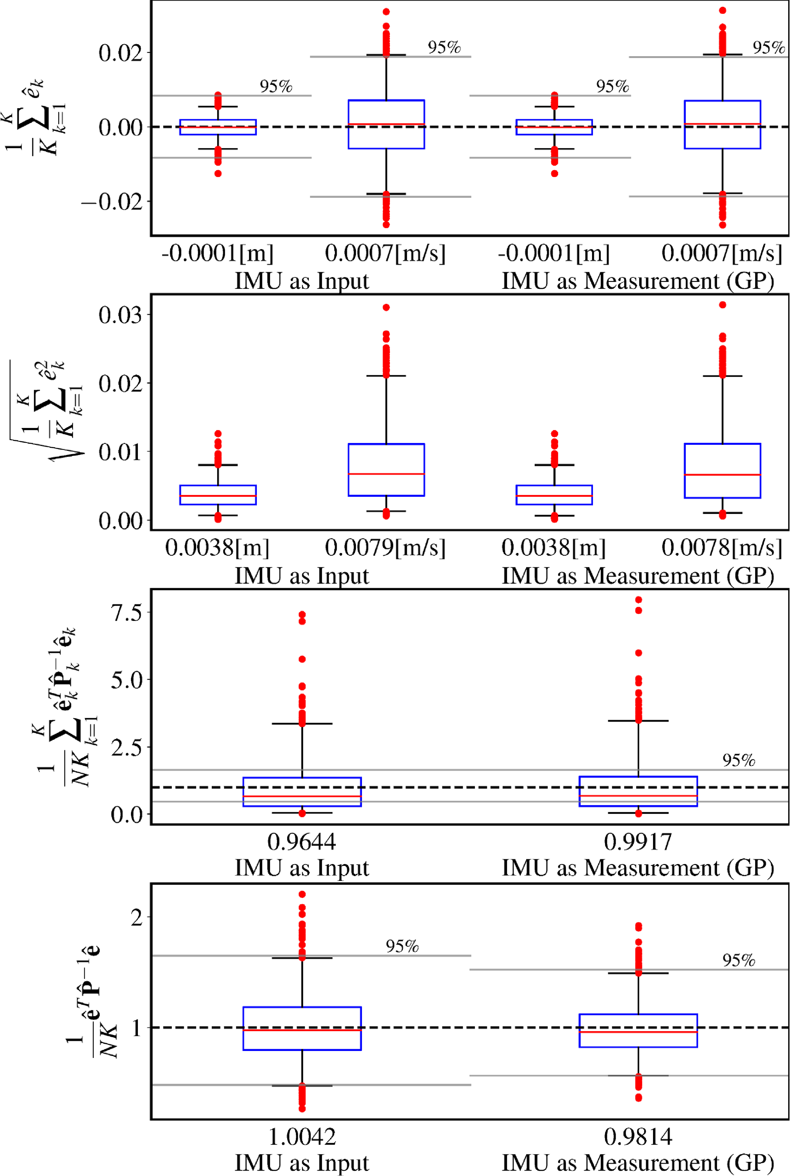
This figure compares the performance of the baseline IMU-as-input approach versus our proposed IMU-as-measurement approach that leverages a Gaussian process (GP) motion prior. The ground-truth trajectories are sampled from a white-noise-on-jerk (WNOJ) prior as shown in Figure 4. The IMU input covariance $Q_k$
for the IMU-as-input method was trained on a validation set, with a value of
$Q_k$
for the IMU-as-input method was trained on a validation set, with a value of $0.00338$
. The parameters of our proposed method was also trained on the same validation set, with resulting values of
$0.00338$
. The parameters of our proposed method was also trained on the same validation set, with resulting values of $\sigma ^2 = 1.0069$
and
$\sigma ^2 = 1.0069$
and $\alpha = 0.0$
.
$\alpha = 0.0$
. $R_{\textrm{pos}}$
for both methods was chosen to match the simulated noise added to the position measurements. Similarly,
$R_{\textrm{pos}}$
for both methods was chosen to match the simulated noise added to the position measurements. Similarly, $R_{\textrm{acc}}$
for the IMU-as-measurement approach was set to match the simulated noise added to the acceleration measurements. In the bottom row, the chi-squared bounds have a different size because the dimension of the state in IMU-as-measurement is greater (it includes acceleration), and so the dimension of the chi-squared distribution increases, resulting in a tighter chi-squared bound.
$R_{\textrm{acc}}$
for the IMU-as-measurement approach was set to match the simulated noise added to the acceleration measurements. In the bottom row, the chi-squared bounds have a different size because the dimension of the state in IMU-as-measurement is greater (it includes acceleration), and so the dimension of the chi-squared distribution increases, resulting in a tighter chi-squared bound.
This figure depicts 1000 simulated trajectories sampled from a singer prior where $\check{\mathbf{x}}_{0} = [0.0\,1.0\,0.0]^T$
,
$\check{\mathbf{x}}_{0} = [0.0\,1.0\,0.0]^T$
, $\check{\mathbf{P}}_{0} = \textrm{diag}(0.001, 0.001, 0.001)$
,
$\check{\mathbf{P}}_{0} = \textrm{diag}(0.001, 0.001, 0.001)$
, $\alpha = 10.0$
, and
$\alpha = 10.0$
, and $\sigma ^2 = 1.0$
. A large value of
$\sigma ^2 = 1.0$
. A large value of $\alpha$
is intended to approximate a white-noise-on-acceleration (WNOA) prior.
$\alpha$
is intended to approximate a white-noise-on-acceleration (WNOA) prior.
This figure summarizes the results of our second simulation experiment where the ground-truth trajectories were sampled from a singer prior with $\alpha = 10.0$
,
$\alpha = 10.0$
, $\sigma ^2 = 1.0$
. The trained acceleration input covariance for IMU-as-input was
$\sigma ^2 = 1.0$
. The trained acceleration input covariance for IMU-as-input was $Q_k \approx 0.00283$
. The trained singer prior parameters were
$Q_k \approx 0.00283$
. The trained singer prior parameters were $\alpha = 10.2442$
and
$\alpha = 10.2442$
and $\sigma ^2 = 1.0074$
. Note that even though the underlying prior changed by a lot from the first simulation to the second, from a white-noise-on-jerk prior to an approximation of a white-noise-on-acceleration prior, both estimators were able to remain unbiased and consistent.
$\sigma ^2 = 1.0074$
. Note that even though the underlying prior changed by a lot from the first simulation to the second, from a white-noise-on-jerk prior to an approximation of a white-noise-on-acceleration prior, both estimators were able to remain unbiased and consistent.
Both IMU-as-input and IMU-as-measurement have parameters that need to be tuned on the dataset. For this purpose, we use a separate training set of 100 sampled trajectories. For the IMU-as-input approach, we learn the covariance of the acceleration input $Q_k$
using maximum likelihood over the training set where we have the benefit of using noiseless ground-truth states in simulation. The objective that we seek to minimize is
$Q_k$
using maximum likelihood over the training set where we have the benefit of using noiseless ground-truth states in simulation. The objective that we seek to minimize is
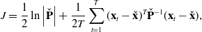 \begin{equation} J = \frac{1}{2}\ln \left | \check{\mathbf{P}} \right | + \frac{1}{2T} \sum _{t=1}^T (\mathbf{x}_t - \check{\mathbf{x}})^T \check{\mathbf{P}}^{-1} (\mathbf{x}_t - \check{\mathbf{x}}), \end{equation}
where $\mathbf{x}_t$
are validation set trajectories,
$\mathbf{x}_t$
are validation set trajectories, $\check{\mathbf{x}} = \mathbf{A} \mathbf{v}$
is the full trajectory prior for the IMU-as-input method,
$\check{\mathbf{x}} = \mathbf{A} \mathbf{v}$
is the full trajectory prior for the IMU-as-input method, $\check{\mathbf{P}} = \mathbf{A}\mathbf{Q}\mathbf{A}^T$
is the prior covariance over the whole trajectory,
$\check{\mathbf{P}} = \mathbf{A}\mathbf{Q}\mathbf{A}^T$
is the prior covariance over the whole trajectory, $\mathbf{A}$
is the lifted transition matrix as in (13),
$\mathbf{A}$
is the lifted transition matrix as in (13), $\mathbf{v}\,=\,\begin{bmatrix} \check{\mathbf{x}}_0^T & \Delta \mathbf{x}_{1, 0}^T & \cdots & \Delta \mathbf{x}_{K, K-1}^T \end{bmatrix}^T$
, and
$\mathbf{v}\,=\,\begin{bmatrix} \check{\mathbf{x}}_0^T & \Delta \mathbf{x}_{1, 0}^T & \cdots & \Delta \mathbf{x}_{K, K-1}^T \end{bmatrix}^T$
, and $\mathbf{Q}\,=\,\textrm{diag}(\check{\mathbf{P}}_0, \boldsymbol{\Sigma }_1, \cdots, \boldsymbol{\Sigma }_K)$
.
$\mathbf{Q}\,=\,\textrm{diag}(\check{\mathbf{P}}_0, \boldsymbol{\Sigma }_1, \cdots, \boldsymbol{\Sigma }_K)$
.
Using a numerical optimizer, we found that $Q_k \approx 0.00338$
given a WNOJ motion prior with
$Q_k \approx 0.00338$
given a WNOJ motion prior with $Qc = 1.0$
, and acceleration measurement noise of
$Qc = 1.0$
, and acceleration measurement noise of $\sigma ^2_{\textrm{acc}} = 0.0001m^2/s^4$
. Note that the input covariance
$\sigma ^2_{\textrm{acc}} = 0.0001m^2/s^4$
. Note that the input covariance $Q_k$
is clearly much greater than the simulated noise on the acceleration measurements
$Q_k$
is clearly much greater than the simulated noise on the acceleration measurements $\sigma ^2_{\textrm{acc}}$
. This is because, for the IMU-as-input approach, the covariance on the acceleration input
$\sigma ^2_{\textrm{acc}}$
. This is because, for the IMU-as-input approach, the covariance on the acceleration input $Q_k$
is conflating two sources of noise, the IMU measurement noise and the underlying process noise. It also means that
$Q_k$
is conflating two sources of noise, the IMU measurement noise and the underlying process noise. It also means that $Q_k$
has to be trained and adapted to new datasets in order to maintain a consistent estimator.
$Q_k$
has to be trained and adapted to new datasets in order to maintain a consistent estimator.
For the IMU-as-measurement approach, we need to train the parameters of our Gaussian process (GP) motion prior. In order to highlight the versatility of our proposed approach, we employ a Singer motion prior [Reference Wong, Yoon, Schoellig and Barfoot30], which has the capacity to model priors ranging from WNOA to WNOJ. The Singer prior is parametrized by an inverse length scale matrix $\boldsymbol{\alpha }$
and a variance
$\boldsymbol{\alpha }$
and a variance $\boldsymbol{\sigma }^2$
, both of which are diagonal. For values of
$\boldsymbol{\sigma }^2$
, both of which are diagonal. For values of $\boldsymbol{\alpha }$
close to zero, numerical optimizers encounter difficulties due to numerical instabilities of
$\boldsymbol{\alpha }$
close to zero, numerical optimizers encounter difficulties due to numerical instabilities of $\mathbf{Q}_k$
and its Jacobians. Instead, we derive the analytical gradients to learn
$\mathbf{Q}_k$
and its Jacobians. Instead, we derive the analytical gradients to learn $\{{\boldsymbol{\alpha }}, \boldsymbol{\sigma }^2\}$
using gradient descent following the approach presented by Wong et al. [Reference Wong, Yoon, Schoellig and Barfoot30]. The objective that we seek to minimize is
$\{{\boldsymbol{\alpha }}, \boldsymbol{\sigma }^2\}$
using gradient descent following the approach presented by Wong et al. [Reference Wong, Yoon, Schoellig and Barfoot30]. The objective that we seek to minimize is
 \begin{equation} J = \frac{1}{2} \sum _{t=1}^T \sum _{k=1}^K \left ( \mathbf{e}_{k,t}^T \mathbf{Q}_{k,t}^{-1} \mathbf{e}_{k,t} + \ln \left | \mathbf{Q}_{k,t} \right | \right ), \end{equation}
where both $\mathbf{e}_{k,t}$
and
$\mathbf{e}_{k,t}$
and $\mathbf{Q}_{k,t}$
are functions of the Singer prior parameters
$\mathbf{Q}_{k,t}$
are functions of the Singer prior parameters $\{{\boldsymbol{\alpha }}, \boldsymbol{\sigma }^2\}$
. Further details on the analytical gradients are provided in the supplementary materials. Note that the approach of Wong et al. [Reference Wong, Yoon, Schoellig and Barfoot30] supports learning the parameters of the Singer prior even with noisy ground truth; however, it requires that we first estimate the measurement covariances and then keep them fixed during the optimization. In order to learn both the GP parameters and the measurement covariances simultaneously, Wong et al. leverage exactly sparse Gaussian variational inference [Reference Wong, Yoon, Schoellig and Barfoot15].
$\{{\boldsymbol{\alpha }}, \boldsymbol{\sigma }^2\}$
. Further details on the analytical gradients are provided in the supplementary materials. Note that the approach of Wong et al. [Reference Wong, Yoon, Schoellig and Barfoot30] supports learning the parameters of the Singer prior even with noisy ground truth; however, it requires that we first estimate the measurement covariances and then keep them fixed during the optimization. In order to learn both the GP parameters and the measurement covariances simultaneously, Wong et al. leverage exactly sparse Gaussian variational inference [Reference Wong, Yoon, Schoellig and Barfoot15].
Figure 5 shows the results of our first simulation experiment with the WNOJ prior. Each row in Figure 5 is a box plot of a metric computed independently for each of the 1000 simulated trajectories. The blue boxes represent the interquartile range, the red lines are the medians, the whiskers correspond to the 2.5 and 97.5 percentiles, and the red dots denote outliers (data points beyond the whiskers). The black dashed lines in the first, third, and fourth rows corresponds to the target value that is 0 for the mean error and 1 for the normalized estimation error squared (NEES). Underneath each box plot, we also compute the mean value of the metrics across all data points.
In the first row of Figure 5, we can see that the mean error in both position and velocity is close to zero for both estimators. The gray lines in the first row denote a 95% two-sided confidence interval, a statistical test to check that the estimators are unbiased. We expect to see the whiskers of the box plots lie within the 95% confidence interval in order to confirm that the estimator is unbiased, which is the case.
The third row displays a commonly used method for computing the NEES. This method uses the marginals of the posterior covariance and relies on the ergodic hypothesis in order to treat the error from each timestep as being independent. In this case, we compute the marginal covariance at each timestep for position and velocity only so that the results of the two estimators can be compared directly. The gray lines denote a 95% chi-squared bound, a statistical test for checking that the estimators are consistent. Interestingly, we observe that neither estimator passes the statistical test in this case, even though the mean and median NEES are close to 1. It appears that, in this case, the ergodic hypothesis is not valid.
In the fourth row, we present an alternative formulation of the NEES that uses the full posterior covariance over the entire trajectory. In this case, we are satisfied to find that both estimators pass the statistical test for confirming that they are consistent. The main difference between this version of the NEES and the previous one is that we have retained the cross-covariance terms between timesteps.
In summary, we observe that the two approaches achieve nearly identical performance. Both estimators are unbiased and consistent so long as their parameters are trained on a training set.
Figures 6, 7 depict the results of our second experiment where the ground-truth trajectories are sampled from a Singer prior with $\alpha = 10.0$
,
$\alpha = 10.0$
, $\sigma ^2 = 1.0$
. This large value of
$\sigma ^2 = 1.0$
. This large value of $\alpha$
is intended to approximate a WNOA prior. Our results show that both estimators are capable of adapting to a dataset with a different underlying motion prior while remaining unbiased and consistent.
$\alpha$
is intended to approximate a WNOA prior. Our results show that both estimators are capable of adapting to a dataset with a different underlying motion prior while remaining unbiased and consistent.
3.6. Discussion
As mentioned previously, the big-O time complexity of classic preintegration and our approach are the same. In practice, our approach is slightly slower but not by much. Using a modern CPU, either approach can be considered real-time capable. Note that the number of preintegration windows could be adjusted and each preintegration window could be computed in parallel to make the approach more efficient. In this way, we could parallelize the solving of some estimation problems. We are motivated by sensor configurations that cannot be easily handled by classic preintegration such as multiple asynchronous high-rate sensors. This could include a lidar and an IMU or multiple asynchronous IMUs.
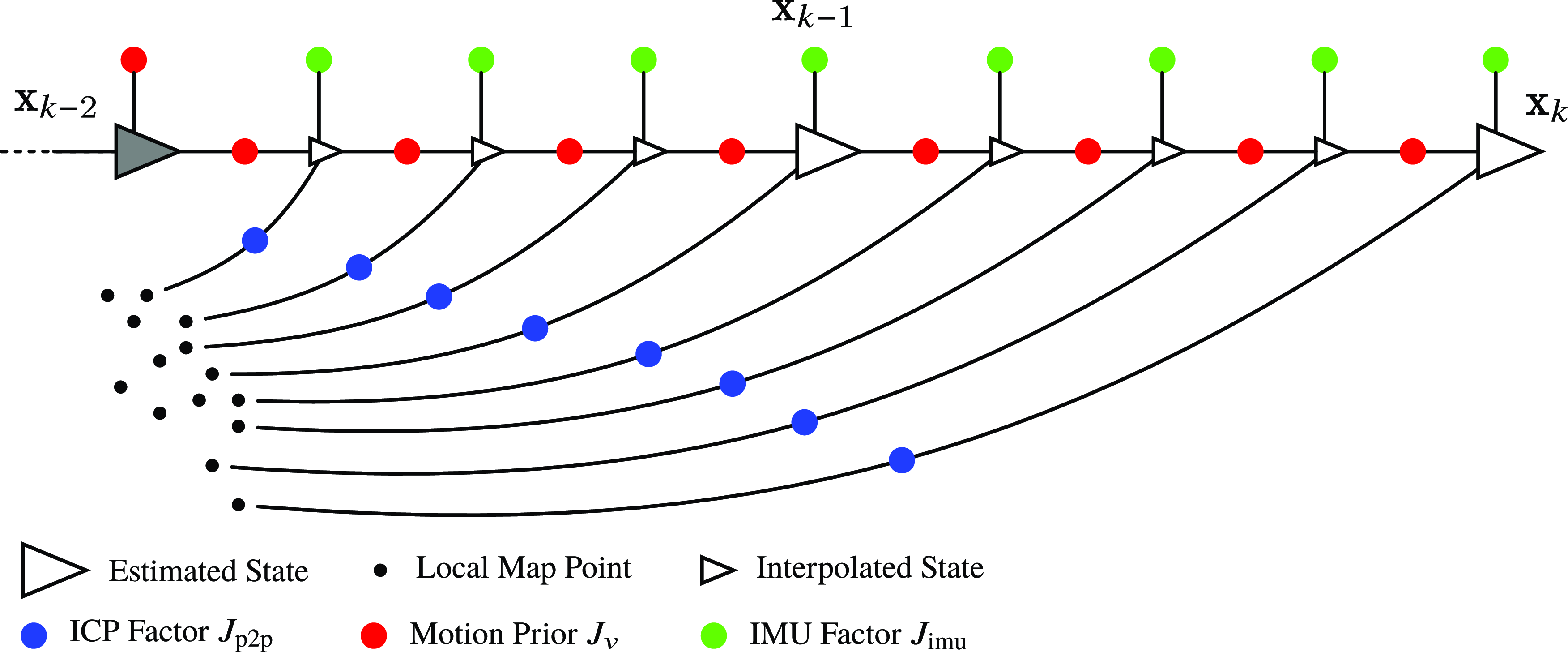
This figure depicts a factor graph of our sliding-window lidar-inertial odometry using a continuous-time motion prior. The larger triangles represent the estimation times that form our sliding window. The state $\mathbf{x}(t) = \{\mathbf{T}(t), \boldsymbol{\varpi }(t), \dot{\boldsymbol{\varpi }}(t), \mathbf{b}(t) \}$
includes the pose
$\mathbf{x}(t) = \{\mathbf{T}(t), \boldsymbol{\varpi }(t), \dot{\boldsymbol{\varpi }}(t), \mathbf{b}(t) \}$
includes the pose $\mathbf{T}(t)$
, the body-centric velocity
$\mathbf{T}(t)$
, the body-centric velocity $\boldsymbol{\varpi }(t)$
, the body-centric acceleration
$\boldsymbol{\varpi }(t)$
, the body-centric acceleration $\dot{\boldsymbol{\varpi }}(t)$
, and the IMU biases
$\dot{\boldsymbol{\varpi }}(t)$
, and the IMU biases $\mathbf{b}(t)$
. The gray-shaded state
$\mathbf{b}(t)$
. The gray-shaded state $\mathbf{x}_{k-2}$
is next to be marginalized and is held fixed during the optimization of the current window. The smaller triangles are interpolated states that we do not directly estimate during the optimization process. Instead, we construct continuous-time measurement factors using the posterior Gaussian process interpolation formula. We include a unary prior on
$\mathbf{x}_{k-2}$
is next to be marginalized and is held fixed during the optimization of the current window. The smaller triangles are interpolated states that we do not directly estimate during the optimization process. Instead, we construct continuous-time measurement factors using the posterior Gaussian process interpolation formula. We include a unary prior on $\mathbf{x}_{k-2}$
to denote the prior information from the sliding-window filter.
$\mathbf{x}_{k-2}$
to denote the prior information from the sliding-window filter.
4. Lidar-inertial odometry
Our lidar-inertial odometry is implemented as sliding-window batch trajectory estimation. The factor graph corresponding to our approach is depicted in Figure 8. The state $\mathbf{x}(t) = \{\mathbf{T}(t), \boldsymbol{\varpi }(t), \dot{\boldsymbol{\varpi }}(t), \mathbf{b}(t)\}$
consists of the
$\mathbf{x}(t) = \{\mathbf{T}(t), \boldsymbol{\varpi }(t), \dot{\boldsymbol{\varpi }}(t), \mathbf{b}(t)\}$
consists of the $SE(3)$
pose
$SE(3)$
pose $\mathbf{T}_{vi}(t)$
, the body-centric velocity
$\mathbf{T}_{vi}(t)$
, the body-centric velocity $\boldsymbol{\varpi }_v^{vi}(t)$
, the body-centric acceleration
$\boldsymbol{\varpi }_v^{vi}(t)$
, the body-centric acceleration $\dot{\boldsymbol{\varpi }}_v^{vi}(t)$
, and the IMU biases
$\dot{\boldsymbol{\varpi }}_v^{vi}(t)$
, and the IMU biases $\mathbf{b}(t)$
.
$\mathbf{b}(t)$
. $\boldsymbol{\varpi }_v^{vi}$
is a
$\boldsymbol{\varpi }_v^{vi}$
is a $6\times 1$
vector containing the body-centric linear velocity
$6\times 1$
vector containing the body-centric linear velocity $\boldsymbol{\nu }_v^{vi}$
and angular velocity
$\boldsymbol{\nu }_v^{vi}$
and angular velocity $\boldsymbol{\omega }_v^{vi}$
. We approximate the
$\boldsymbol{\omega }_v^{vi}$
. We approximate the $SE(3)$
trajectory using a sequence of local Gaussian processes as in [Reference Anderson and Barfoot28]. Between pairs of estimation times, the local variable
$SE(3)$
trajectory using a sequence of local Gaussian processes as in [Reference Anderson and Barfoot28]. Between pairs of estimation times, the local variable $\boldsymbol{\xi }_k(t)$
is defined as:
$\boldsymbol{\xi }_k(t)$
is defined as:
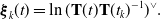 \begin{equation} \boldsymbol{\xi }_k(t) = \ln (\mathbf{T}(t) \mathbf{T}(t_k)^{-1})^\vee . \end{equation}
We use (32) and the following to convert between global and local variables:
 \begin{align} \dot{\boldsymbol{\xi }}_k(t) &={\boldsymbol{\mathcal{J}}}(\boldsymbol{\xi }_k(t))^{-1} \boldsymbol{\varpi }(t), \\[-2pt] \nonumber \end{align}
 \begin{align} \ddot{\boldsymbol{\xi }}_k(t) &\approx -\frac{1}{2}({\boldsymbol{\mathcal{J}}}({\boldsymbol{\xi }}_k(t))^{-1}{\boldsymbol{\varpi }}(t))^\curlywedge{\boldsymbol{\varpi }}(t) +{\boldsymbol{\mathcal{J}}}({\boldsymbol{\xi }}_k(t))^{-1} \dot{{\boldsymbol{\varpi }}}(t), \\[12pt] \nonumber \end{align}
where the approximation for $\ddot{\boldsymbol{\xi }}_k(t)$
was originally derived by Tang et al. [Reference Tang, Yoon and Barfoot14]. We use a Singer prior, introduced in [Reference Wong, Yoon, Schoellig and Barfoot30], which is defined by the following Gaussian process:
$\ddot{\boldsymbol{\xi }}_k(t)$
was originally derived by Tang et al. [Reference Tang, Yoon and Barfoot14]. We use a Singer prior, introduced in [Reference Wong, Yoon, Schoellig and Barfoot30], which is defined by the following Gaussian process:
 \begin{equation} \ddot{{\boldsymbol{\xi }}}_k(t) \sim \mathcal{GP}(\mathbf{0}, \boldsymbol{\sigma }^2 \exp\! ({-}\boldsymbol{\ell }^{-1}|t - t^\prime |)), \end{equation}
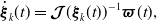
and which can equivalently be represented using the following LTI SDE:
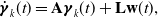 \begin{align} \dot{\boldsymbol{\gamma }}_k(t) &= \mathbf{A} \boldsymbol{\gamma }_k(t) + \mathbf{L} \mathbf{w}(t), \end{align}
where
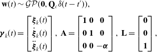 \begin{align*} \mathbf{w}(t) &\sim \mathcal{GP}(\mathbf{0}, \mathbf{Q}_c \delta (t - t^\prime )), \\[3pt] \boldsymbol{\gamma }_k(t) &= \begin{bmatrix} \boldsymbol{\xi }_k(t) \\[3pt] \dot{\boldsymbol{\xi }}_k(t) \\[3pt] \ddot{\boldsymbol{\xi }}_k(t) \end{bmatrix},\,\mathbf{A} = \begin{bmatrix} \mathbf{1} & \mathbf{0} & \mathbf{0} \\[3pt] \mathbf{0}& \mathbf{1} & \mathbf{0} \\[3pt] \mathbf{0}& \mathbf{0} & -\boldsymbol{\alpha } \end{bmatrix},\,\mathbf{L} = \begin{bmatrix} \mathbf{0} \\[3pt] \mathbf{0} \\[3pt] \mathbf{1} \end{bmatrix}, \end{align*} $\boldsymbol{\sigma }^2$
is a variance,
$\boldsymbol{\sigma }^2$
is a variance, $\boldsymbol{\ell }$
is a length scale,
$\boldsymbol{\ell }$
is a length scale, $\boldsymbol{\alpha } = \boldsymbol{\ell }^{-1}$
, and
$\boldsymbol{\alpha } = \boldsymbol{\ell }^{-1}$
, and $\mathbf{w}(t)$
is a white-noise Gaussian process where
$\mathbf{w}(t)$
is a white-noise Gaussian process where $\mathbf{Q}_c = 2\boldsymbol{\alpha }\boldsymbol{\sigma }^2$
is the associated power spectral density matrix. (36) can be stochastically integrated to arrive at a local Gaussian process:
$\mathbf{Q}_c = 2\boldsymbol{\alpha }\boldsymbol{\sigma }^2$
is the associated power spectral density matrix. (36) can be stochastically integrated to arrive at a local Gaussian process:
 \begin{align} \boldsymbol{\gamma }_k(t) \sim \mathcal{GP}(&\boldsymbol{\Phi }(t, t_k) \check{\boldsymbol{\gamma }}_k(t_k)), \boldsymbol{\Phi }(t, t_k) \check{\mathbf{P}}(t_k) \boldsymbol{\Phi }(t, t_k)^T +{\mathbf{Q}_t} ), \end{align}
where the formulation for the transition function $\boldsymbol{\Phi }(t, t_k)$
and the covariance
$\boldsymbol{\Phi }(t, t_k)$
and the covariance $\mathbf{Q}_t$
can be found in [Reference Wong, Yoon, Schoellig and Barfoot30]. In order to convert our continuous-time formulation into a factor graph, we build a sequence of motion prior factors between pairs of estimation times using
$\mathbf{Q}_t$
can be found in [Reference Wong, Yoon, Schoellig and Barfoot30]. In order to convert our continuous-time formulation into a factor graph, we build a sequence of motion prior factors between pairs of estimation times using
 \begin{align} J_{v,k} &= \frac{1}{2} \mathbf{e}_{v,k}^T \mathbf{Q}_k^{-1} \mathbf{e}_{v,k}, \\[-2pt] \nonumber \end{align}
 \begin{align} \mathbf{e}_{v,k} &= \boldsymbol{\gamma }_k(t_{k+1}) - \boldsymbol{\Phi }(t_{k+1}, t_k) \boldsymbol{\gamma }_k(t_k). \\[12pt] \nonumber \end{align}
Our IMU measurement model is
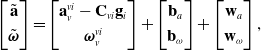 \begin{equation} \begin{bmatrix} \tilde{\mathbf{a}} \\[3pt] \tilde{\boldsymbol{\omega }} \end{bmatrix} = \begin{bmatrix} \mathbf{a}_v^{vi} - \mathbf{C}_{vi}\mathbf{g}_i \\[3pt] \boldsymbol{\omega }_v^{vi} \end{bmatrix} + \begin{bmatrix} \mathbf{b}_a \\[3pt] \mathbf{b}_{\omega } \end{bmatrix} + \begin{bmatrix} \mathbf{w}_a \\[3pt] \mathbf{w}_{\omega } \end{bmatrix}, \end{equation}
where $\mathbf{b}_a$
and
$\mathbf{b}_a$
and $\mathbf{b}_\omega$
are the accelerometer and gyroscope biases,
$\mathbf{b}_\omega$
are the accelerometer and gyroscope biases, $\mathbf{w}_a \sim \mathcal{N}(\mathbf{0}, \mathbf{R}_{a})$
and
$\mathbf{w}_a \sim \mathcal{N}(\mathbf{0}, \mathbf{R}_{a})$
and $\mathbf{w}_\omega \sim \mathcal{N}(\mathbf{0}, \mathbf{R}_{\omega })$
are zero-mean Gaussian noise. Due to angular velocity and acceleration being a part of the state, the associated IMU error function is straightforward:
$\mathbf{w}_\omega \sim \mathcal{N}(\mathbf{0}, \mathbf{R}_{\omega })$
are zero-mean Gaussian noise. Due to angular velocity and acceleration being a part of the state, the associated IMU error function is straightforward:
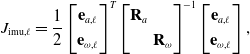 \begin{align} J_{\textrm{imu}, \ell } &={\frac{1}{2} \begin{bmatrix} \mathbf{e}_{a,\ell } \\[3pt] \mathbf{e}_{\omega, \ell } \end{bmatrix}^T \begin{bmatrix} \mathbf{R}_a & \\[3pt] & \mathbf{R}_\omega \end{bmatrix}^{-1} \begin{bmatrix} \mathbf{e}_{a,\ell } \\[3pt] \mathbf{e}_{\omega, \ell } \end{bmatrix},} \\[-2pt] \nonumber \end{align}
 \begin{align} \mathbf{e}_{a,\ell } &= \tilde{\mathbf{a}}_\ell - \dot{\boldsymbol{\nu }}(\tau _\ell ) + \mathbf{C}_{vi}(\tau _\ell ) \mathbf{g}_i -\mathbf{b}_{a}(\tau _\ell ), \\[-2pt] \nonumber \end{align}
 \begin{align} \mathbf{e}_{\omega, \ell } &= \tilde{\boldsymbol{\omega }}_\ell - \boldsymbol{\omega }(\tau _{\ell }) - \mathbf{b}_{\omega }(\tau _{\ell }),\\[12pt] \nonumber \end{align}
where we rely on forming measurement factors using the posterior Gaussian process interpolation formula. For each of these continuous-time measurement factors, we compute Jacobians of the perturbation to the state at the interpolated times with respect to the bracketing estimation times. This is an approximation, as it is not exactly the same as marginalization. However, we have found it to work well in practice. We also include motion prior factors for the IMU biases:
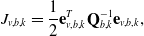 \begin{align} J_{v,b,k} &= \frac{1}{2} \mathbf{e}_{v,b,k}^T \mathbf{Q}_{b,k}^{-1} \mathbf{e}_{v,b,k}, \\[-2pt] \nonumber \end{align}
 \begin{align} \mathbf{e}_{v,b,k} &= \mathbf{b}(t_{k+1}) - \mathbf{b}(t_{k}), \\[12pt] \nonumber \end{align}
where $\mathbf{Q}_{b,k} = \boldsymbol{Q}_b \Delta t_k$
is the covariance resulting from a white-noise-on-velocity motion prior and
$\mathbf{Q}_{b,k} = \boldsymbol{Q}_b \Delta t_k$
is the covariance resulting from a white-noise-on-velocity motion prior and $\boldsymbol{Q}_b$
is the associated power spectral density matrix. We use point-to-plane factors. The associated error function is
$\boldsymbol{Q}_b$
is the associated power spectral density matrix. We use point-to-plane factors. The associated error function is
 \begin{align} J_{\textrm{p2p},j} &= \mathbf{e}_{\textrm{p2p},j}^T \mathbf{R}_{\textrm{p2p},j}^{-1} \mathbf{e}_{\textrm{p2p},j}, \\[-2pt] \nonumber \end{align}
 \begin{align} \mathbf{e}_{\textrm{p2p},j} &={\alpha _j} \mathbf{n}_j^T \mathbf{D} (\mathbf{p}_j - \mathbf{T}_{vi}(\tau _j)^{-1} \mathbf{T}_{vs} \mathbf{q}_j), \\[12pt] \nonumber \end{align}
where $\mathbf{q}_j$
is the query point,
$\mathbf{q}_j$
is the query point, $\mathbf{p}_j$
is the matched point in the local map,
$\mathbf{p}_j$
is the matched point in the local map, $\mathbf{n}_j$
is an estimate of the surface normal at
$\mathbf{n}_j$
is an estimate of the surface normal at $\mathbf{p}_j$
given neighboring points in the map,
$\mathbf{p}_j$
given neighboring points in the map, $\mathbf{D}$
is a constant matrix removing the homogeneous component,
$\mathbf{D}$
is a constant matrix removing the homogeneous component, $\mathbf{T}_{vs}$
is a known extrinsic calibration between the lidar frame and the vehicle frame, and
$\mathbf{T}_{vs}$
is a known extrinsic calibration between the lidar frame and the vehicle frame, and ${\alpha _j} = (\sigma _2 - \sigma _3)/\sigma _1$
[Reference Dellenbach, Deschaud, Jacquet and Goulette31] is a heuristic weight to favor planar neighborhoods. The objective function that we seek to minimize is
${\alpha _j} = (\sigma _2 - \sigma _3)/\sigma _1$
[Reference Dellenbach, Deschaud, Jacquet and Goulette31] is a heuristic weight to favor planar neighborhoods. The objective function that we seek to minimize is
 \begin{equation} J = \sum _k J_{v,k} + \sum _j J_{\textrm{p2p},j} + \sum _\ell J_{\textrm{imu},\ell }. \end{equation}
We solve this nonlinear least squares problem for the optimal perturbation to the state using Gauss-Newton. Once the solver has converged, we update the pointcloud correspondences and iterate this two-step process to convergence. In practice, we typically limit the maximum number of inner-loop Gauss-Newton iterations to 10, and the number of outer-loop iterations to 10 in order to enable real-time operation.
In our approach, we estimate the orientation of the gravity vector relative to the initial map frame at startup. We perform sliding-window batch trajectory estimation where the length of the sliding window is $200$
ms. We output the pose at the middle of the newest lidar scan.
$200$
ms. We output the pose at the middle of the newest lidar scan.
5. IMU-as-input lidar-inertial baseline
As a baseline where IMU measurements are treated as an input, we consider a lidar-inertial odometry approach where IMU measurements are used to de-skew the lidar pointcloud and classic preintegration is used as a prior. The baseline is implemented as sliding-window batch trajectory estimation and the factor graph corresponding to the baseline approach is depicted in Figure 9. The state $\mathbf{x}(t_k) = \{\mathbf{C}_{iv}(t_k), \mathbf{r}_i^{vi}(t_k), \mathbf{v}^{vi}_i(t_k), \mathbf{b}(t_k) \}$
consists of the orientation
$\mathbf{x}(t_k) = \{\mathbf{C}_{iv}(t_k), \mathbf{r}_i^{vi}(t_k), \mathbf{v}^{vi}_i(t_k), \mathbf{b}(t_k) \}$
consists of the orientation $\mathbf{C}_{iv}(t_k)$
, position
$\mathbf{C}_{iv}(t_k)$
, position $\mathbf{r}_i^{vi}(t_k)$
, velocity
$\mathbf{r}_i^{vi}(t_k)$
, velocity $\mathbf{v}^{vi}_i(t_k)$
, and IMU biases. All variables are expressed in a global frame. We use classic preintegration to form binary factors between pairs of estimated states in the sliding window [Reference Forster, Carlone, Dellaert and Scaramuzza2]. At each iteration of the optimization, we integrate the IMU measurements to extrapolate for the state at each IMU measurement time using
$\mathbf{v}^{vi}_i(t_k)$
, and IMU biases. All variables are expressed in a global frame. We use classic preintegration to form binary factors between pairs of estimated states in the sliding window [Reference Forster, Carlone, Dellaert and Scaramuzza2]. At each iteration of the optimization, we integrate the IMU measurements to extrapolate for the state at each IMU measurement time using
 \begin{align} \mathbf{C}_j &= \mathbf{C}_i \prod _{k=i}^{j-1} \exp \left (\Delta t_k (\tilde{\boldsymbol{\omega }}_k - \mathbf{b}_\omega (t_k))^\wedge \right ), \\[-8pt] \nonumber \end{align}
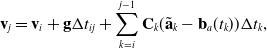 \begin{align} \mathbf{v}_j &= \mathbf{v}_i + \mathbf{g} \Delta t_{ij} + \sum _{k=i}^{j-1} \mathbf{C}_k (\tilde{\mathbf{a}}_k - \mathbf{b}_a(t_k)) \Delta t_k, \\[-8pt] \nonumber \end{align}
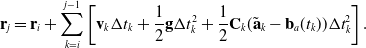 \begin{align} \mathbf{r}_j &= \mathbf{r}_i + \sum _{k=i}^{j-1} \left [ \mathbf{v}_k \Delta t_k + \frac{1}{2} \mathbf{g} \Delta t_k^2 + \frac{1}{2}\mathbf{C}_k (\tilde{\mathbf{a}}_k - \mathbf{b}_a(t_k)) \Delta t_k^2 \right ]. \\[12pt] \nonumber \end{align}
The position at a given lidar point time can then be obtained by linearly interpolating between the positions at the IMU measurement times. The orientation at a given lidar point time can be obtained using the following formula:
 \begin{equation} \mathbf{C}(\tau _j) = \mathbf{C}(t_\ell ) \left (\mathbf{C}(t_\ell )^T \mathbf{C}(t_{\ell +1}) \right )^\alpha \end{equation}
where $\alpha = (\tau _j - t_\ell ) / (t_{\ell +1} - t_\ell )$
. Using these interpolated states, we can write the point-to-plane error function as:
$\alpha = (\tau _j - t_\ell ) / (t_{\ell +1} - t_\ell )$
. Using these interpolated states, we can write the point-to-plane error function as:
 \begin{equation} \mathbf{e}_{\textrm{p2p},j} = \mathbf{n}_j^T \left (\mathbf{p}_j - \mathbf{C}_{iv}(\tau _j)(\mathbf{C}_{vs}\mathbf{q}_j +\mathbf{r}_v^{sv}) - \mathbf{r}_i^{vi}(\tau _j) \right ). \end{equation}
The Jacobians of this error function with respect to perturbations to the state variables are provided in the appendix.
This figure depicts a factor graph of our baseline approach that uses IMU measurements to de-skew the pointcloud and to form relative motion priors using classic preintegration. The larger triangles represent the estimation times that form our sliding window. The state $\mathbf{x}(t_k) = \{\mathbf{C}_{iv}(t_k), \mathbf{r}_i^{vi}(t_k), \mathbf{v}^{vi}_i(t_k), \mathbf{b}(t_k) \}$
includes the orientation and position in a global frame, the velocity in a global frame, and the IMU biases. The gray-shaded state
$\mathbf{x}(t_k) = \{\mathbf{C}_{iv}(t_k), \mathbf{r}_i^{vi}(t_k), \mathbf{v}^{vi}_i(t_k), \mathbf{b}(t_k) \}$
includes the orientation and position in a global frame, the velocity in a global frame, and the IMU biases. The gray-shaded state $\mathbf{x}_{k-2}$
is next to be marginalized. The smaller triangles are extrapolated states that we do not directly estimate during the optimization process. Instead, we extrapolate for these states using IMU integration starting at an estimated state. The factor graph includes a unary prior on
$\mathbf{x}_{k-2}$
is next to be marginalized. The smaller triangles are extrapolated states that we do not directly estimate during the optimization process. Instead, we extrapolate for these states using IMU integration starting at an estimated state. The factor graph includes a unary prior on $\mathbf{x}_{k-2}$
to denote the prior information from the sliding-window filter.
$\mathbf{x}_{k-2}$
to denote the prior information from the sliding-window filter.
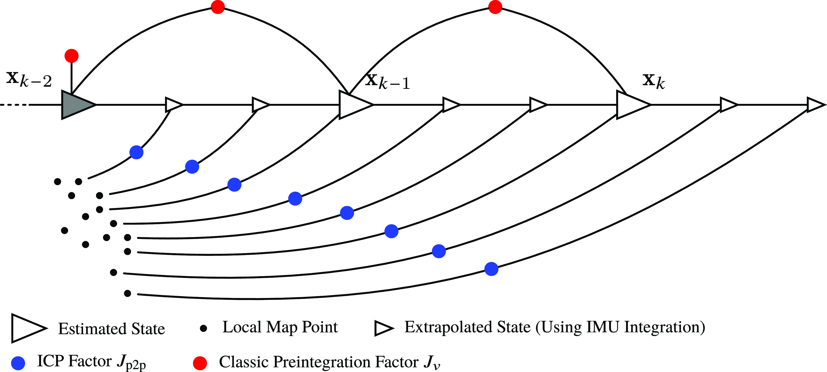
6. Lidar-inertial simulation
In this section, we compare the performance of our lidar-inertial odometry to the baseline imu-as-input approach in a simulated environment. The simulated environment is a rectangular room, and we simulate trajectories using sinusoidal body-centric velocities:
 \begin{equation} \left [{\boldsymbol{\varpi }}(t)\right ]_j = A_j \sin\! (2\pi f_j t), \end{equation}
where $A_j$
and
$A_j$
and $f_j$
are configurable amplitude and frequency parameters. The resulting body-centric acceleration can be obtained via differentiation:
$f_j$
are configurable amplitude and frequency parameters. The resulting body-centric acceleration can be obtained via differentiation:
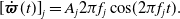 \begin{equation} \left [\dot{{\boldsymbol{\varpi }}}(t)\right ]_j = A_j 2\pi f_j \cos\! (2\pi f_j t). \end{equation}
We then step through the simulation so as to replicate the lidar firing sequence of a Velodyne Alpha-Prime 128-beam lidar, obtaining the pose of the sensor for each firing sequence. Starting with $\mathbf{T}_0 = \mathbf{T}_{vi}(t_0) = \mathbf{1}$
,
$\mathbf{T}_0 = \mathbf{T}_{vi}(t_0) = \mathbf{1}$
,
 \begin{equation} \mathbf{T}_{k+1} \approx \exp \left ( \left ({\boldsymbol{\varpi }}(t_k)\Delta t_k + \frac{1}{2} \Delta t_k^2 \dot{{\boldsymbol{\varpi }}}(t_k)\right )^\wedge \right ) \mathbf{T}_{k}, \end{equation}
where $\Delta t_k$
is very small (53.3
$\Delta t_k$
is very small (53.3 $\mu$
s). By generating the trajectories in this way, it is straightforward to extract the body-centric angular velocity and linear acceleration to simulate IMU measurements. We use the measurement model in (39) to simulate biases and gravity components. We simulate a constant nonzero bias on each gyroscope and accelerometer axis. We include zero-mean Gaussian noise on IMU measurements as well as Gaussian noise on the range measurement of each lidar point. We chose measurement noises to be close to what we experience on our experimental platform. Figure 10 depicts an example pointcloud produced in our simulation environment where the points are colored based off which wall they are reflected. Figure 11 compares the trajectory estimated by our lidar-inertial odometry with the ground truth.
$\mu$
s). By generating the trajectories in this way, it is straightforward to extract the body-centric angular velocity and linear acceleration to simulate IMU measurements. We use the measurement model in (39) to simulate biases and gravity components. We simulate a constant nonzero bias on each gyroscope and accelerometer axis. We include zero-mean Gaussian noise on IMU measurements as well as Gaussian noise on the range measurement of each lidar point. We chose measurement noises to be close to what we experience on our experimental platform. Figure 10 depicts an example pointcloud produced in our simulation environment where the points are colored based off which wall they are reflected. Figure 11 compares the trajectory estimated by our lidar-inertial odometry with the ground truth.
This figure depicts an example lidar pointcloud produced by our simulation, which contains motion distortion. The pointcloud is colored based off which wall the lidar point is reflected.
This figure depicts the results of our lidar-inertial simulation where the ground-truth position (dashed line) is compared to the position estimated by Singer-LIO colored by the absolute position error. This trajectory is an example of one of the slow sequences.
For the simulation parameters, we use an IMU rate of 200 Hz, a simulation length of 20s, and three motion regimes denoted slow, medium, and fast. Where for each of these motion regimes, we randomly sample for the amplitudes and frequencies of the body-centric velocities used in the simulation of a sequence. The ranges for these parameters is given in Table I. One set of amplitudes and frequencies is sampled for each of the 20 sequences simulated for the three motion regimes. We set the standard deviation of the accelerometer measurement noise to 0.02 $\textrm{m/s}^2$
, the standard deviation of the gyroscope measurement noise to 0.01 rad/s, and the standard deviation of the lidar range measurements to 0.02 m. The accelerometers were given a constant bias of 0.05
$\textrm{m/s}^2$
, the standard deviation of the gyroscope measurement noise to 0.01 rad/s, and the standard deviation of the lidar range measurements to 0.02 m. The accelerometers were given a constant bias of 0.05 $\textrm{m/s}^2$
, and the gyroscopes were given a constant bias of 0.05 rad/s.
$\textrm{m/s}^2$
, and the gyroscopes were given a constant bias of 0.05 rad/s.
We compare the performance of our lidar-inertial odometry against the baseline in Table II where we also show the performance of our approach using only the lidar and the gyroscope, and lidar only. We obtained the results by computing the absolute trajectory error between our estimated trajectories and the ground truth using the evo evaluation tool.1 The results in the table are the overall root mean squared error obtained by concatenating the error from each individual sequence. The results show that in the low speed regime, the imu-as-input baseline approach and our imu-as-measurement approach based on the Singer prior achieve nearly identical results. This is unsurprising as it appears to replicate the results from Section 3.5. Interestingly, our lidar-only approach performs the best on the slow regime. However, in the medium and fast regime, the advantage of our lidar-inertial approach becomes apparent. In the medium regime, the baseline imu-as-input approach begins to break down. This is possibly due to the fact that the motion is no longer approximately constant acceleration and constant angular rate. On the other hand, our lidar-inertial approach performs roughly the same in the medium regime. Our lidar-only approach also breaks down in the medium regime. In the fast regime, both our lidar-inertial and lidar with gyro approaches achieve respectable results, while the lidar-only approach and the imu-as-input baseline fail completely.
Simulation parameter ranges for the different motion regimes.
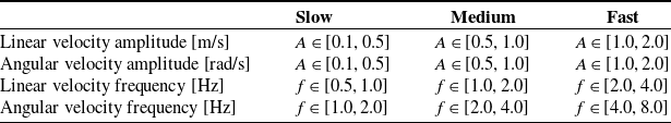
Simulation results. Root mean squared absolute trajectory error (m). For each speed category (slow, medium, and fast), 20 randomized sequences were created. The results in this table are the overall root mean squared absolute position error across 20 sequences, for each approach.
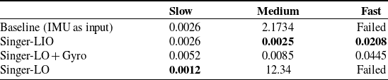
7. Experimental results
In this section, we provide experimental results on the Newer College Dataset [Reference Ramezani, Wang, Camurri, Wisth, Mattamala and Fallon32]. This dataset features a 64-beam Ouster lidar and provides the internal IMU measurements of the Ouster lidar. Ground-truth poses were obtained by matching live lidar poses to a map of the environment created using a survey-grade lidar at several stationary poses. This dataset is somewhat unique in that it features several sequences with highly dynamic motions. In Table III, we compare the performance of using our continuous-time Singer prior using lidar only (Singer-LO), lidar and a gyroscope only (Singer-LO + Gyro), and a full lidar-inertial setup including an accelerometer (Singer-LIO). We also compare the performance of our approach to some comparable works in the literature such as CT-ICP [Reference Dellenbach, Deschaud, Jacquet and Goulette31], a lidar-only approach, FAST-LIO2 [Reference Xu, Cai, He, Lin and Zhang20] and DLIO [Reference Chen, Nemiroff and Lopez21], which can be considered the prior state of the art for this dataset, and SLICT [Reference Nguyen, Duberg, Jensfelt, Yuan and Xie33] and CLIO [Reference Lv, Lang, Xu, Wang, Liu and Zuo8], which are two continuous-time approaches that use linear interpolation and B-splines, respectively.
Newer College Dataset results. Root mean squared absolute trajectory error (m). Estimated trajectory aligned with ground truth using Umeyama algorithm. * uses loop closures, † results obtained from [Reference Chen, Nemiroff and Lopez21], ‡ uses camera images.
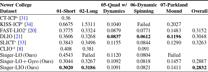
Our approach, Singer-LIO, demonstrates the best performance on the 01-Short and 02-Long sequences and also demonstrates the best overall performance. Interestingly, the sequences in which we expected the IMU to make the most difference were 05-Quad w/ Dynamics and 06-Dynamic Spinning due to their dynamic motions. However, we observe that in these sequences, our lidar-only approach performs similarly or even better, replicating the results of our lidar-inertial simulation. It appears that, in this dataset, the addition of an IMU mainly helps in areas where there are geometric degeneracies rather than the areas with dynamic motions. Sequences 05-Quad w/ Dynamics and 06-Dynamic Spinning are very similar to our lidar-inertial simulation in the slow regime, as they are conducted in a rectangular quad at New College, Oxford. FAST-LIO2 and DLIO can be considered state-of-the-art IMU-as-input approaches, and our approach demonstrates a clear advantage over these methods.
8. Conclusions
In this work, we compared treating an IMU as an input to a motion model versus treating it as a measurement of the state. On a 1D simulation problem, we showed that these two approaches performed identically when the data are sampled from either a constant velocity or constant acceleration prior and both methods are trained on a hold-out set. We demonstrated our approach to continuous-time lidar-inertial odometry using the Singer prior where body-centric acceleration is included in the state. In our simulated environment, we showed that our lidar-inertial odometry outperformed lidar-only odometry and an IMU-as-input baseline approach. On the Newer College Dataset, we demonstrated state-of-the-art resuts. There is still plenty of work to be done in treating IMU measurements as measurements of the state. Similar to nonuniform B-splines, it would be interesting to investigate a setup where the parameters of the Singer prior are adjusted on the fly so as to adjust between periods of smooth versus highly dynamic motion. When the IMU is treated as a measurement of the state, this allows us to now incorporate exogenous control inputs into our Gaussian process motion prior. This could be a promising area of research for estimating the state of drones where the torque commanded to the motors is often known. Our approach to combine multiple asynchronous high-rate sensors may prove beneficial in other sensor configurations such as multiple asynchronous IMUs.
Author contributions
Keenan Burnett carried out the research and wrote the article, Angela Schoellig provided feedback on research, and Tim Barfoot conceived of the study and provided feedback on research.
Financial support
This work was supported in part by the National Sciences and Engineering Research Council of Canada (NSERC) and by an Ontario Research Fund: Research Excellence (ORF-RE) grant.
Competing interests
The authors declare none.
Data availability
Data sharing is not applicable to this article as no new data were created or analyzed in this study.
Supplementary material
The supplementary material for this article can be found at https://doi.org/10.1017/S0263574724002121.


 Open access