





1. Introduction
The development of multicellular organisms, cell migration and information processing by nerve cells in the brain depends on various interactions between the cells and other biological factors. In these phenomena, the functions of these interactions determine the state of the subsequent time evolution and exhibit the occurrence and various behaviour of the patterns. When modelling such phenomena, there are cases in which long-range interactions that affect distant objects globally in space naturally appear. These interactions are called nonlocal interactions. They have attracted considerable attention in various fields and have been studied extensively. The existence of nonlocal interactions has been experimentally suggested, for example, in phenomena such as neural firing in the brain [Reference Kuffler13], pigmentation patterns in animal skin [Reference Nakamasu, Takahashi, Kanbe and Kondo18, Reference Watanabe and Kondo22, Reference Yamanaka and Kondo23], development of multicellular organisms, cell migration and adhesion [Reference Katsunuma, Honda and Shinoda11].
In the experiment by Kuffler [Reference Kuffler13], the electrode was set at a ganglion cell in the receptive field of the retina of a cat. The firing rate against the light stimulus was measured by illuminating two points at different distances from the electrodes. Ganglion cells respond to light stimuli locally in space and, conversely, inhibit them laterally in space. From these observations, by considering the local excitation and lateral inhibition as positive and negative values, respectively, this interaction can be modelled by a sign-change function with radial symmetry. This function is called the local activation and lateral inhibition (LALI) interaction or Mexican hat.
Experimental results on the interactions between yellow and black pigment cells in the skin of zebrafish were reported by Nakamasu et al. [Reference Nakamasu, Takahashi, Kanbe and Kondo18]. During these experiments, a square section of black pigmented cells within a zebrafish’s skin stripe was eliminated using laser ablation. The regions of yellow pigmented cells surrounding the squares were removed by laser ablation. Several zebrafish were prepared with different patterns of yellow pigmented cells, which were removed using a laser. For each pattern of yellow pigment cells, the number of black pigment cells proliferating in the square located at the centre of the pattern was quantified for two weeks. The comparison of the number of proliferating black pigment cells revealed the existence of both long- and short-range interactions between these cells. Moreover, the derived interactions are summarised as a network. A theoretical method to reduce a given reaction-diffusion network with spatial interactions, such as metabolites or signals with arbitrary factors, into the shape of an essential integral kernel has been proposed by Ei et al. [Reference Ei, Ishii, Kondo, Miura and Tanaka9]. A Mexican hat function was theoretically derived by applying this reduction method to the network given by Nakamasu et al. [Reference Nakamasu, Takahashi, Kanbe and Kondo18]. Additionally, cells such as the pigment cells in the zebrafish extend their cellular projections to exchange the biological signals with each other. Here, we refer to the papers by Katsunuma et al. [Reference Katsunuma, Honda and Shinoda11] and Kondo [Reference Kondo12]. Hamada et al. [Reference Hamada, Watanabe and Lau14] and Watanabe and Kondo [Reference Watanabe and Kondo22] reported that pigment cells send different biological signals depending on the length of their cellular projections.
Katsunuma et al. [Reference Katsunuma, Honda and Shinoda11] investigated the behaviour of cell adhesion by using two types of cellular adhesion molecules in HEK 293 cells. These cells also have cellular projections that are ten times longer than their body size. Cells can sense the cell density around them using their total body from the tip of the leading edge, and they can decide the directions of cell migration and cell adhesion.
Based on this biological background, numerous mathematical models have been proposed and analysed. The nonlocal interactions are often modelled by convolution with a suitable integral kernel. Here, we introduce two types of the model of the nonlocal interaction. We call the convolution itself without a derivative the normal type, and the gradient of convolution in the advection term the advective type. We introduce mathematical models with a normal type of nonlocal interaction. The peaks of biological signals are located distantly from the centre of the cell body during signal transduction through cellular projections. Here, we refer to the observational results of Hamada et al. [Reference Hamada, Watanabe and Lau14] and Watanabe and Kondo [Reference Watanabe and Kondo22]. For these interactions, many models that impose a convolution with an integral kernel with peaks distant from the origin have been proposed. For example, as models of pigmentation patterns in animal skin [Reference Ninomiya, Tanaka and Yamamoto19, Reference Ninomiya, Tanaka and Yamamoto20], population dispersal for biological individuals [Reference Ei, Guo, Ishii and Wu8, Reference Hutson, Martinez, Mischaikow and Vickers15], and vegetation patterns [Reference Alfaro, Izuhara and Mimura1], the following nonlocal evolution equation is proposed:
 \begin{equation*} u_t = d\Delta u +K * u +f( u ), \end{equation*}
where $d \ge 0$
is a constant,
$d \ge 0$
is a constant, $u=u(x,t)$
is the density,
$u=u(x,t)$
is the density, $f$
is a suitable reaction or growth term,
$f$
is a suitable reaction or growth term, $K$
is an integral kernel and
$K$
is an integral kernel and $*$
denotes the convolution of two functions in the space variable:
$*$
denotes the convolution of two functions in the space variable:
 \begin{equation*} K*u (x,t) = \int K(x-y) u(y,t) dy. \end{equation*}
Analytical results were reported by Bates et al. [Reference Bates, Fife, Ren and Wang4], Coville et al. [Reference Coville, Dávila and Martíanez7] and Ei et al. [Reference Ei, Guo, Ishii and Wu8]. It is rigorously shown by Ninomiya et al. [Reference Ninomiya, Tanaka and Yamamoto19] that the nonlocal interaction plays a role to induce the Turing instability. By imposing a convolution using the Heaviside function, a nonlocal evolution equation to investigate the dynamics of the membrane potential of neurones in the brain was proposed by Amari [Reference Amari2]. Additionally, motivated by the pattern formations observed in animal skins, a nonlocal model by applying the cut function to the convolution term was proposed by Kondo [Reference Kondo12]. This model can reproduce various patterns by changing only the kernel shape, even though it comprises only one component. The above nonlocal interactions can be derived from the continuation of spatially discretised models with intercellular interactions by Ei et al. [Reference Ei, Ishii, Sato, Tanaka, Wang and Yasugi10].
Next, we introduce mathematical models of the advective type of nonlocal interaction. As a first example, the aggregation-diffusion equation was proposed and analysed for cell migration and collective motion by Bailo et al. [Reference Bailo, Carrillo, Murakawa and Schmidtchen3] and Carrillo et al. [Reference Carrillo, Craig and Yao5]:
 \begin{equation} \rho _t = \Delta \rho ^m - \nabla \cdot (\rho \nabla ( W* \rho ) ), \quad m\ge 1, \end{equation}
where $\rho =\rho (x,t)$
denotes the cell density at position
$\rho =\rho (x,t)$
denotes the cell density at position $x$
at time
$x$
at time $t\gt 0$
and
$t\gt 0$
and $m\ge 1$
is a constant. If the potential
$m\ge 1$
is a constant. If the potential $W$
is positive, the convolution term
$W$
is positive, the convolution term $\nabla ( W* \rho )$
determines the velocity of the advection by integrating the gradient of
$\nabla ( W* \rho )$
determines the velocity of the advection by integrating the gradient of $\rho$
. The density
$\rho$
. The density $\rho$
at each point is advected towards the gradient of
$\rho$
at each point is advected towards the gradient of $\rho$
. Thus, the second term provides the aggregation effect. If
$\rho$
. Thus, the second term provides the aggregation effect. If $W$
is positive with a compact support, then the compact support corresponds to the total cell body. Subsequently, the term
$W$
is positive with a compact support, then the compact support corresponds to the total cell body. Subsequently, the term $\nabla ( W* \rho )$
provides the effect that determines the velocity of the advection by sensing the cell density gradient in the total cell body. When
$\nabla ( W* \rho )$
provides the effect that determines the velocity of the advection by sensing the cell density gradient in the total cell body. When $m=1$
, this model can be classified as a nonlocal Fokker–Planck equation, whereas when
$m=1$
, this model can be classified as a nonlocal Fokker–Planck equation, whereas when $m\gt 1$
, it can be classified as a nonlocal porous medium equation.
$m\gt 1$
, it can be classified as a nonlocal porous medium equation.
Another example is the cell adhesion model. It has been proposed to describe and analyse the cell adhesion phenomena by Carrillo et al. [Reference Carrillo, Murakawa, Sato, Togashi and Trush6]:
 \begin{equation} \rho _t = \Delta \rho ^2 - \nabla \cdot (\rho (1-\rho )\nabla ( W*\rho ))+f(\rho ). \end{equation}
In contrast to the aggregation-diffusion equation, the velocity in the advection term is saturated by the cell density $(1-\rho )$
in this model. Carrillo et al. [Reference Carrillo, Murakawa, Sato, Togashi and Trush6] reported that this model can replicate cell adhesion and cell sorting phenomena both qualitatively and quantitatively. For cell migration and cell adhesion processes, the integral kernel is called the potential, and the Mexican hat (or LALI) function is crucial in the local attraction and lateral repulsion in these two models.
$(1-\rho )$
in this model. Carrillo et al. [Reference Carrillo, Murakawa, Sato, Togashi and Trush6] reported that this model can replicate cell adhesion and cell sorting phenomena both qualitatively and quantitatively. For cell migration and cell adhesion processes, the integral kernel is called the potential, and the Mexican hat (or LALI) function is crucial in the local attraction and lateral repulsion in these two models.
Cell pattern formation, migration, and adhesion play pivotal roles in the biological development of various organs and tissues. Therefore, revealing the mechanisms underlying these phenomena is an important problem. However, the nonlocal term with the normal or advection type in nonlocal equations occasionally makes analysis difficult. To overcome this difficulty, the approximation of a nonlocal term by another type of term can be a solution. In light of this, we aim to reveal whether advective nonlocal interactions can be approximated by local dynamics. As a first step, we propose an approximation method for advective nonlocal terms in the nonlocal Fokker–Planck equation using a Keller–Segel system with multiple auxiliary chemotactic factors. Although the above models of (1.1) and (1.2) are considered in higher-dimensional spaces, we consider the problem on one-dimensional bounded domain in the simple case to make the regularity of the solution and fundamental solution to the elliptic equation in quasi-steady state easier to deal with. The nonlocal Fokker–Planck equation and Keller–Segel systems are basic models with advective nonlocal interactions and typical local dynamics, respectively. We show that any smooth kernel can be expanded by combining the fundamental solutions for an elliptic equation in the Keller–Segel system. Furthermore, we report that the solution to the nonlocal Fokker–Planck equation with an even smooth kernel can be approximated by that of the Keller–Segel system with specified parameters depending on the integral kernel shape. The equations used to approximate nonlocal interactions are reaction-diffusion equations, and this idea is the same as that of Ninomiya et al. [Reference Ninomiya, Tanaka and Yamamoto19, Reference Ninomiya, Tanaka and Yamamoto20]. In these papers, the results of approximation by the singular limit of the reaction-diffusion system for nonlocal interactions of normal type in one-dimensional space are reported. This is based on a theory to approximate the integral kernel by a linear sum of fundamental solutions to an elliptic equation of second order. In contrast, for the approximation of advective nonlocal interactions, it is necessary to approximate the derivative of the integral kernel by a linear sum of the aforementioned fundamental solutions, as in Corollary 2.6 below. The $C^1$
estimate is the essential difference and difficulty between this approximation problem and the previous studies. To prove this convergence, we provide an estimation of the approximation using the Lagrange interpolation polynomial with the Chebyshev nodes. This enables us to evaluate the relationship between the error accuracy and the number of equations in the approximation.
$C^1$
estimate is the essential difference and difficulty between this approximation problem and the previous studies. To prove this convergence, we provide an estimation of the approximation using the Lagrange interpolation polynomial with the Chebyshev nodes. This enables us to evaluate the relationship between the error accuracy and the number of equations in the approximation.
The remainder of this paper is organised as follows: Section 2 outlines the mathematical framework and summarises the main results. In Section 3, the existence theorem is established, followed by a singular limit analysis detailed in Section 4. Section 5 starts by presenting a precise formula for the Lagrange interpolation polynomial’s coefficient. This is followed by a method to ascertain the coefficient of the linear sum in the fundamental solution for an elliptic equation, characterised by the shape of its integral kernel. The section also includes a proof of the fundamental solution’s series expansion. A linear stability analysis is then conducted in Section 6. The paper concludes with Section 7, summarising the study’s findings and implications.
2. Mathematical settings and main results
In this section, we describe the mathematical settings and results. We denote the theoretical concentration or cell density at position $x \in \Omega \,:\!=\, [-L , L]$
at time
$x \in \Omega \,:\!=\, [-L , L]$
at time $t\gt 0$
by
$t\gt 0$
by $\rho = \rho (x,t)$
. We investigate the solution to the following nonlocal Fokker–Planck equation:
$\rho = \rho (x,t)$
. We investigate the solution to the following nonlocal Fokker–Planck equation:
 \begin{equation} \rho _ t = \rho _{xx} - ( \rho ( W*\rho )_x )_x \ \text{in} \ \Omega \times (0,\infty ), \end{equation}
where the periodic boundary condition
 \begin{equation} \left \{ \begin{aligned} &\rho (-L,t) = \rho (L, t), \ t\gt 0, \\ &\rho _x(-L, t) = \rho _x( L, t), \ t\gt 0, \end{aligned} \right . \end{equation}
is imposed and the initial datum is given by $\rho (x, 0) \,:\!=\, \rho _0(x)$
. Here,
$\rho (x, 0) \,:\!=\, \rho _0(x)$
. Here, $W*u(x)$
is defined by
$W*u(x)$
is defined by
 \begin{equation*} W*u (x) \,:\!=\, \int _\Omega W(x-y) u(y) dy \end{equation*}
for $W \in L^1_{\mathrm{per}}(\Omega ) \,:\!=\, \{u|_\Omega \in L^1(\Omega ) \ | \ u(x)=u(x+2L), \ x \in {\mathbb{R}} \}$
. Setting
$W \in L^1_{\mathrm{per}}(\Omega ) \,:\!=\, \{u|_\Omega \in L^1(\Omega ) \ | \ u(x)=u(x+2L), \ x \in {\mathbb{R}} \}$
. Setting $d_j\gt 0, (j=1,\ldots , M)$
which are the diffusion coefficients in (
$d_j\gt 0, (j=1,\ldots , M)$
which are the diffusion coefficients in ( $\mbox{KS}^{M,\varepsilon }$
) introduced below, we define the following function
$\mbox{KS}^{M,\varepsilon }$
) introduced below, we define the following function
 \begin{equation} k_j(x)\,:\!=\, \frac {1}{2\sqrt {d_j} \sinh \frac {L}{\sqrt {d_j} } } \cosh \frac {L - \left | x \right |}{\sqrt { d_j } }. \end{equation}
This is actually a fundamental solution to the elliptic equation explained in Lemma 4.1 below. The typical examples of $W$
are as follows:
$W$
are as follows:
 \begin{align} &W(x) = k_1(x) \text{ with any } d_1\gt 0, \end{align}
 \begin{align} &W(x) = k_1(x) - k_2(x) \text{ with any } d_1\lt d_2, \end{align}
 \begin{align} &W(x) = (R_0 - |x| )\chi _{B(R_0)}(x), \end{align}
 \begin{align} &W(x) = ((a_1+a_2)R_0 -a_2R_1 -a_1 |x| )\chi _{B(R_0)}(x) - a_2(R_1-|x|)\chi _{ B(R_1)\backslash B(R_0) }(x) \end{align}
with any $a_1, a_2\gt 0$
, where
$a_1, a_2\gt 0$
, where $R_1\gt R_0\gt 0$
are constants called the sensing radius,
$R_1\gt R_0\gt 0$
are constants called the sensing radius, $B(R_0)$
is a ball with radius
$B(R_0)$
is a ball with radius $R_0$
and origin centre, and
$R_0$
and origin centre, and
 \begin{equation*} \chi _{B(R_0)}(x)= \left \{ \begin{aligned} &1 \ & \text{if} \ x \in B(R_0),\\ &0 \ & \text{otherwise}. \end{aligned} \right .\\ \end{equation*}
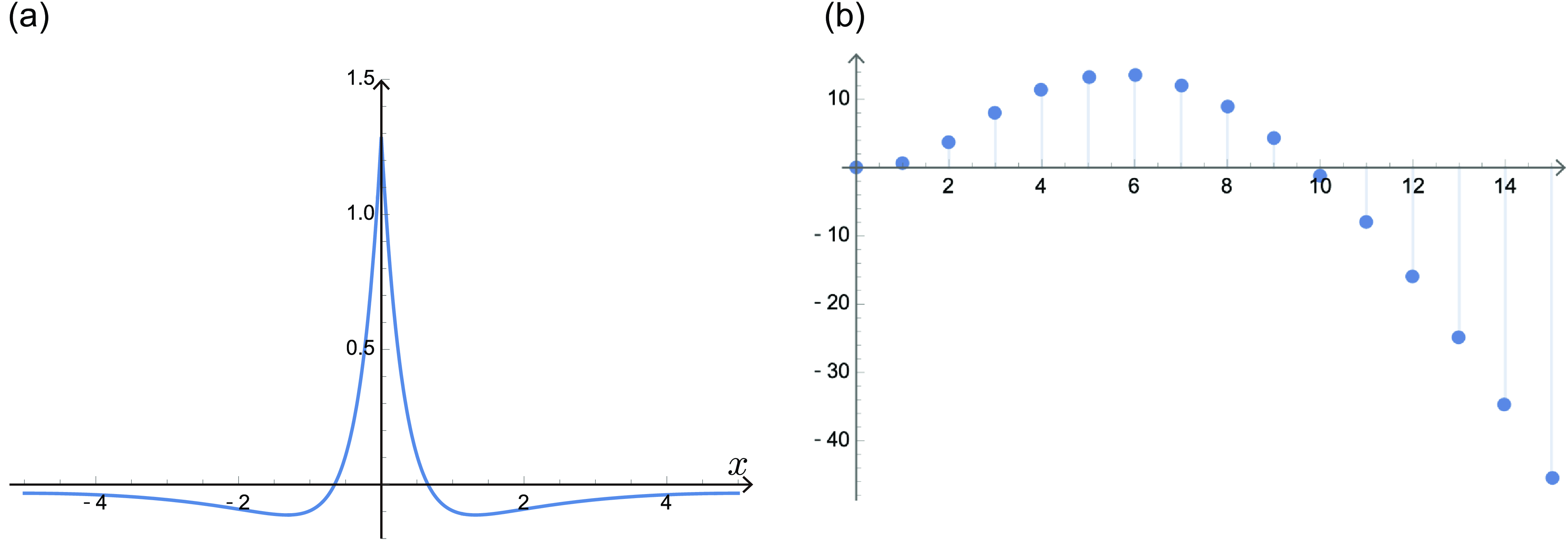
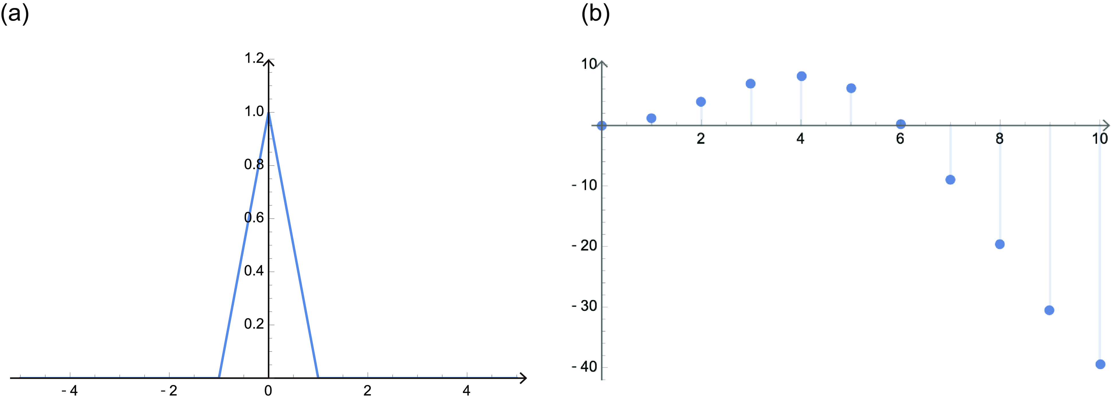
The profiles of (2.6) and (2.7) are presented in Figures 1 (a) and 2 (a), respectively. The nonlocal Fokker–Planck equation (P) with the integral kernels (2.5) and (2.6) corresponds to the parabolic-elliptic Keller–Segel systems. A linear stability analysis is presented in Section 6. Integral kernels (2.7) and (2.8) were introduced by Carrillo et al. [Reference Carrillo, Murakawa, Sato, Togashi and Trush6] and Murakawa and Togashi [Reference Murakawa and Togashi17]. They have a compact support corresponding to the cell body. If these integral kernels are used for the potential $W$
in (P), this describes the situation in which
$W$
in (P), this describes the situation in which $\rho$
at each point detects the surrounding cell density in the own cell body and the velocity of the aggregation is determined. This corresponds to the Haptotaxis phenomenon.
$\rho$
at each point detects the surrounding cell density in the own cell body and the velocity of the aggregation is determined. This corresponds to the Haptotaxis phenomenon.


First, we have the following existence result. To construct a mild solution to (P), we define a function space with a norm as
 \begin{equation*} E_{\tau }\,:\!=\, C([0, \tau ]; H^1(\Omega )), \quad \left \| \cdot \right \|_{ E_{\tau } } \,:\!=\, \left \| \cdot \right \|_{ C([0, \tau ];H^1 (\Omega ))} \end{equation*}
for any time $\tau \gt 0$
. Introducing the following function:
$\tau \gt 0$
. Introducing the following function:
 \begin{align} G(x,t) \,:\!=\, \frac {1 }{2L } \sum _{n \in \mathbb{Z}} e^{-\sigma _n^2 t} e^{i\sigma _n x}, \end{align}
where $i$
is the imaginary unit and
$i$
is the imaginary unit and
 \begin{equation*} \sigma _n \,:\!=\, \frac {n \pi }{L}, \quad n \in \mathbb{Z}, \end{equation*}
we define the map $\Gamma \,{:}\, E_{\tau } \to E_{\tau }$
as
$\Gamma \,{:}\, E_{\tau } \to E_{\tau }$
as
 \begin{align*} \Gamma [u] (x,t) \,:\!=\, (G * \rho _0)(x,t) - \int _0^t \int _\Omega G(x-y, t-s) ( u (W*u)_x )_x(y, s) dy ds, \quad u \in E_{\tau }. \end{align*}
We say that a function $u \in C([0,T]; H^1(\Omega ))$
for any
$u \in C([0,T]; H^1(\Omega ))$
for any $T\gt 0$
is a mild solution to (P) with
$T\gt 0$
is a mild solution to (P) with $\rho (x,0)=\rho _0(x)$
, provided
$\rho (x,0)=\rho _0(x)$
, provided $ u=\Gamma [u]$
. The following proposition is proven using the standard argument of the fixed point theorem.
$ u=\Gamma [u]$
. The following proposition is proven using the standard argument of the fixed point theorem.
Proposition 2.1.
Let $R\gt 0$
be an arbitrary real number, and assume that
$R\gt 0$
be an arbitrary real number, and assume that $W \in W_{\mathrm{per}}^{1,1}(\Omega )\,:\!=\,\{u|_\Omega \in W^{1,1}(\Omega ) \ | \ u(x)=u(x+2L), \ x \in {\mathbb{R}} \}$
and
$W \in W_{\mathrm{per}}^{1,1}(\Omega )\,:\!=\,\{u|_\Omega \in W^{1,1}(\Omega ) \ | \ u(x)=u(x+2L), \ x \in {\mathbb{R}} \}$
and
 \begin{align*} \rho _0 \in H^1(\Omega ) \ \text{with} \ \left \| \rho _0 \right \|_{H^1(\Omega )} \lt R. \end{align*}
Then, for any $T\gt 0$
, there exists a unique mild solution
$T\gt 0$
, there exists a unique mild solution $\rho$
to (
P
) in
$\rho$
to (
P
) in $ C( [0, T]; H^1(\Omega ) ) \cap L^2( 0, T; H^2(\Omega ) )$
satisfying
$ C( [0, T]; H^1(\Omega ) ) \cap L^2( 0, T; H^2(\Omega ) )$
satisfying
 \begin{equation*} \left \| \rho \right \|_{C([0, T], H^1 (\Omega ))} \lt C_0, \end{equation*}
where $C_0 =C_0(L,R,T, \|W_x\|_{L^1(\Omega )} )$
. Moreover, this mild solution satisfies (P) in
$C_0 =C_0(L,R,T, \|W_x\|_{L^1(\Omega )} )$
. Moreover, this mild solution satisfies (P) in $L^2(0,T;L^2(\Omega ))$
.
$L^2(0,T;L^2(\Omega ))$
.
Next, we will approximate the solution to (P) with any integral kernel using that to a Keller–Segel system which is a local dynamics. Introducing the auxiliary factors $v_j^{M,\varepsilon } = v_j^{M,\varepsilon }(x,t), \ (j=1, \ldots , M)$
, we consider the following Keller–Segel system in which the linear sum of
$v_j^{M,\varepsilon } = v_j^{M,\varepsilon }(x,t), \ (j=1, \ldots , M)$
, we consider the following Keller–Segel system in which the linear sum of $v_j^{M,\varepsilon }$
is imposed in nonlocal term in (P):
$v_j^{M,\varepsilon }$
is imposed in nonlocal term in (P):
 \begin{equation*} \left \{ \begin{aligned} \rho ^{M,\varepsilon }_t & = \rho ^{M,\varepsilon }_{xx} - \left( \rho ^{M,\varepsilon } \left( \sum _{j=1}^M a_j v_j^{M,\varepsilon } \right)_x \right)_x,\\ (v_j^{M,\varepsilon } )_t &= \frac {1}{\varepsilon } \left( d_j \left( v_{j}^{M,\varepsilon } \right)_{xx} - v_j^{M,\varepsilon } + \rho ^{M,\varepsilon } \right), \ (j=1,\cdots , M) \end{aligned} \right . \ \text{in} \ \Omega \times (0,\infty ).\qquad\qquad\qquad\quad\ \ \qquad (\text{KS}^{M,\varepsilon }) \end{equation*}
Here, $0 \lt \varepsilon \ll 1$
is a sufficiently small parameter,
$0 \lt \varepsilon \ll 1$
is a sufficiently small parameter, $d_j \gt 0$
is the diffusion coefficient, and each
$d_j \gt 0$
is the diffusion coefficient, and each $a_j \in {\mathbb{R}}$
is a constant that determines whether
$a_j \in {\mathbb{R}}$
is a constant that determines whether $v_j^{M,\varepsilon }$
acts as an attractive or repulsive substance in the aggregation process of
$v_j^{M,\varepsilon }$
acts as an attractive or repulsive substance in the aggregation process of $\rho ^{M,\varepsilon }$
. Because the solutions to (
$\rho ^{M,\varepsilon }$
. Because the solutions to ( $\mbox{KS}^{M,\varepsilon }$
) depends on
$\mbox{KS}^{M,\varepsilon }$
) depends on $M$
and
$M$
and $\varepsilon$
, we denoted them by
$\varepsilon$
, we denoted them by $(\rho ^{M,\varepsilon }, v_j^{M,\varepsilon })$
, respectively. The same periodic boundary condition as that in (P) is imposed in the equations of (
$(\rho ^{M,\varepsilon }, v_j^{M,\varepsilon })$
, respectively. The same periodic boundary condition as that in (P) is imposed in the equations of ( $\mbox{KS}^{M,\varepsilon }$
) as follows:
$\mbox{KS}^{M,\varepsilon }$
) as follows:
 \begin{equation} \left \{ \begin{aligned} &\rho ^{M,\varepsilon }(-L,t) = \rho ^{M,\varepsilon }(L, t), \ t\gt 0, \\ &\rho ^{M,\varepsilon }_x(-L, t) = \rho ^{M,\varepsilon }_x( L, t), \ t\gt 0,\\ &v_j^{M,\varepsilon }(-L,t) = v_j^{M,\varepsilon }(L,t), \ t\gt 0, \\ &\left(v_j^{M,\varepsilon }\right)_x(-L,t) = \left(v_j^{M,\varepsilon }\right)_x(L,t), \ t\gt 0 \\ \end{aligned} \right . \end{equation}
for $j=1, \ldots , M$
. Furthermore, we impose the following initial conditions as
$j=1, \ldots , M$
. Furthermore, we impose the following initial conditions as
 \begin{equation} \rho ^{M,\varepsilon } (x, 0) \,:\!=\,\rho _0^{M,\varepsilon }(x) = \rho _0(x), \quad v_j^{M,\varepsilon }(x, 0) \,:\!=\, ( v_{j})_0(x), \quad (j=1, \ldots , M). \end{equation}
( $\mbox{KS}^{M,\varepsilon }$
) is a Keller–Segel system with multiple components with the linear sensitivity function. The role of
$\mbox{KS}^{M,\varepsilon }$
) is a Keller–Segel system with multiple components with the linear sensitivity function. The role of $v_j^{M,\varepsilon }$
can be distinguished by the sign of the coefficient
$v_j^{M,\varepsilon }$
can be distinguished by the sign of the coefficient $a_j$
. If
$a_j$
. If $a_j\gt 0$
, then
$a_j\gt 0$
, then $v_j^{M,\varepsilon }$
is an attractive substance for
$v_j^{M,\varepsilon }$
is an attractive substance for $\rho ^{M,\varepsilon }$
and
$\rho ^{M,\varepsilon }$
and $\rho ^{M,\varepsilon }$
aggregates toward to the region in which the gradient of
$\rho ^{M,\varepsilon }$
aggregates toward to the region in which the gradient of $v_j^{M,\varepsilon }$
is high independently on the value of its concentration. In contrast, if
$v_j^{M,\varepsilon }$
is high independently on the value of its concentration. In contrast, if $a_j\lt 0$
,
$a_j\lt 0$
, $v_j^{M,\varepsilon }$
acts as a repulsive substance for
$v_j^{M,\varepsilon }$
acts as a repulsive substance for $\rho ^{M,\varepsilon }$
, and
$\rho ^{M,\varepsilon }$
, and $\rho ^{M,\varepsilon }$
migrates away from the region in which the gradient of
$\rho ^{M,\varepsilon }$
migrates away from the region in which the gradient of $v_j^{M,\varepsilon }$
is high.
$v_j^{M,\varepsilon }$
is high.
Introducing the following function:
 \begin{align} &G^\varepsilon _j(x,t) \,:\!=\, \frac {1 }{2L } \sum _{n \in \mathbb{Z}} e^{ - \frac { d_j \sigma _n^2 + 1 }{ \varepsilon }t } e^{i\sigma _n x}, \end{align}
we define the maps $\Psi _j: E_{\tau } \to E_{\tau }$
and
$\Psi _j: E_{\tau } \to E_{\tau }$
and $\Phi : E_{\tau } \to E_{\tau }$
as
$\Phi : E_{\tau } \to E_{\tau }$
as
 \begin{align} &\Psi _j[u](x,t) \,:\!=\, (G_j^\varepsilon * (v_j)_0)(x,t) + \frac {1}{\varepsilon } \int _0^t \int _\Omega G_j^\varepsilon ( x -y, t-s ) u (y, s) dy ds, \quad u \in E_{\tau },\\[-10pt]\nonumber \end{align}
 \begin{align} &\Phi [u] (x,t) \,:\!=\, (G * \rho _0)(x,t) - \int _0^t \int _\Omega G(x-y, t-s) \left( u \left( \sum _{j=1}^M a_j \Psi _j[u] \right)_x \right)_x (y, s) dy ds, \quad u \in E_{\tau }, \end{align}
respectively. We now define the scalar integral equation of ( $\mbox{KS}^{M,\varepsilon }$
) as
$\mbox{KS}^{M,\varepsilon }$
) as $\rho ^{M,\varepsilon } = \Phi [\rho ^{M,\varepsilon }]$
. We say that a function
$\rho ^{M,\varepsilon } = \Phi [\rho ^{M,\varepsilon }]$
. We say that a function $(u,\{v_j\}_j) \in C([0,T]; H^1(\Omega ))\times C( [0, T]; C^2(\Omega ) )$
for any
$(u,\{v_j\}_j) \in C([0,T]; H^1(\Omega ))\times C( [0, T]; C^2(\Omega ) )$
for any $T\gt 0$
is a mild solution to (
$T\gt 0$
is a mild solution to ( $\mbox{KS}^{M,\varepsilon }$
) with (2.11), provided
$\mbox{KS}^{M,\varepsilon }$
) with (2.11), provided $ u=\Phi [u]$
and
$ u=\Phi [u]$
and $v_j=\Psi _j[u]$
for
$v_j=\Psi _j[u]$
for $j=1,\ldots ,M$
.
$j=1,\ldots ,M$
.
With the above settings, we obtain a unique solution to ( $\mbox{KS}^{M,\varepsilon }$
) using the fixed point argument.
$\mbox{KS}^{M,\varepsilon }$
) using the fixed point argument.
Theorem 2.2.
Let $R\gt 0$
be an arbitrary real number and assume
$R\gt 0$
be an arbitrary real number and assume
 \begin{align} & \rho _0\in H^1(\Omega ) \ \text{with } \left \| \rho _0 \right \|_{H^1(\Omega )} \lt R,\\[-10pt]\nonumber \end{align}
 \begin{align} & ( v_{j})_0\in C^2(\Omega ), \quad j=1, \ldots , M. \end{align}
Then, there exists a real positive number $\tau _0=\tau _0(M, \{a_j,d_j\}_{j=1}^M, L, R)$
such that for any
$\tau _0=\tau _0(M, \{a_j,d_j\}_{j=1}^M, L, R)$
such that for any $\varepsilon \gt 0$
there exists a unique mild solution
$\varepsilon \gt 0$
there exists a unique mild solution $(\rho ^{M,\varepsilon }, \{ v_j^{M,\varepsilon } \}_{j=1}^M)$
to (
$(\rho ^{M,\varepsilon }, \{ v_j^{M,\varepsilon } \}_{j=1}^M)$
to ( $\mbox{KS}^{M,\varepsilon }$
) in
$\mbox{KS}^{M,\varepsilon }$
) in $ C( [0, \tau _0]; H^1(\Omega ) ) \times C( [0, \tau _0]; C^2(\Omega ) )$
satisfying
$ C( [0, \tau _0]; H^1(\Omega ) ) \times C( [0, \tau _0]; C^2(\Omega ) )$
satisfying
 \begin{equation*} \left \| \rho ^{M,\varepsilon } \right \|_{ C([0, \tau _0]; H^1 (\Omega ))} \lt 2R. \end{equation*}
We can extend the existence time of the solution to an arbitrary time $T$
as follows:
$T$
as follows:
Corollary 2.3.
Suppose the same assumption of Theorem
2.2
. For any $T\gt 0$
, there exists a positive constant
$T\gt 0$
, there exists a positive constant $\tilde {C}_0=\tilde {C}_0(\tau _0,T)$
such that there exists a unique mild solution
$\tilde {C}_0=\tilde {C}_0(\tau _0,T)$
such that there exists a unique mild solution $(\rho ^{M,\varepsilon }, \{v_j^{M,\varepsilon }\}_{j=1}^M)$
to (
$(\rho ^{M,\varepsilon }, \{v_j^{M,\varepsilon }\}_{j=1}^M)$
to ( $\mbox{KS}^{M,\varepsilon }$
) in
$\mbox{KS}^{M,\varepsilon }$
) in $ C( [0, T]; H^1(\Omega ) ) \cap L^2( 0, T; H^2(\Omega ) ) \cap H^1(0,T;L^2(\Omega )) \times C( [0, T]; C^2(\Omega ) )\cap L^2( 0, T; H^3(\Omega ) )\cap H^1( 0, T; L^2(\Omega ) )$
satisfying
$ C( [0, T]; H^1(\Omega ) ) \cap L^2( 0, T; H^2(\Omega ) ) \cap H^1(0,T;L^2(\Omega )) \times C( [0, T]; C^2(\Omega ) )\cap L^2( 0, T; H^3(\Omega ) )\cap H^1( 0, T; L^2(\Omega ) )$
satisfying
 \begin{equation*} \left \| \rho ^{M,\varepsilon } \right \|_{ C([0,T]; H^1 (\Omega ))} \lt \tilde {C}_0. \end{equation*}
Moreover, this mild solution $(\rho ^{M,\varepsilon }, \{v_j^{M,\varepsilon }\}_{j=1}^M)$
satisfies the system (
$(\rho ^{M,\varepsilon }, \{v_j^{M,\varepsilon }\}_{j=1}^M)$
satisfies the system ( $\mbox{KS}^{M,\varepsilon }$
) in
$\mbox{KS}^{M,\varepsilon }$
) in $L^2(0,T;L^2(\Omega ))\times L^2(0,T;C(\Omega ))$
.
$L^2(0,T;L^2(\Omega ))\times L^2(0,T;C(\Omega ))$
.
In order to show the relationship between the solutions of nonlocal Fokker–Planck equation (P) with any potential $W$
and the Keller–Segel system (
$W$
and the Keller–Segel system ( $\mbox{KS}^{M,\varepsilon }$
), we first investigate the relationship between the solution to (P) with the potential provided by
$\mbox{KS}^{M,\varepsilon }$
), we first investigate the relationship between the solution to (P) with the potential provided by $W= \sum _{j=1}^M a_j k_j$
and the solution to (
$W= \sum _{j=1}^M a_j k_j$
and the solution to ( $\mbox{KS}^{M,\varepsilon }$
).
$\mbox{KS}^{M,\varepsilon }$
).
Theorem 2.4.
Let $M$
be an arbitrary fixed natural number, and
$M$
be an arbitrary fixed natural number, and $\rho$
be a solution to (P) equipped with
$\rho$
be a solution to (P) equipped with $W = \sum _{j=1}^M a_j k_j$
and the initial value
$W = \sum _{j=1}^M a_j k_j$
and the initial value $\rho _0 \in C^2(\Omega )$
. Let
$\rho _0 \in C^2(\Omega )$
. Let $\rho ^{M,\varepsilon }$
be a solution to (
$\rho ^{M,\varepsilon }$
be a solution to ( $\mbox{KS}^{M,\varepsilon }$
) equipped with
$\mbox{KS}^{M,\varepsilon }$
) equipped with
 \begin{align} & \rho ^{M,\varepsilon } _0 = \rho _0,\\[-10pt]\nonumber\end{align}
 \begin{align} &( (v_{1})_0, \ldots , (v_{M})_0 ) = ( k_1*\rho _0, \ldots , k_M*\rho _0) . \end{align}
Then, for any $T\gt 0$
, there exist positive constants
$T\gt 0$
, there exist positive constants $C_1$
and
$C_1$
and $C_2$
that depend on
$C_2$
that depend on $M$
,
$M$
, $\{a_j,d_j\}_{j=1}^M$
,
$\{a_j,d_j\}_{j=1}^M$
, $L$
,
$L$
, $R$
and
$R$
and $T$
such that for any
$T$
such that for any $\varepsilon \gt 0$
 \begin{align} &\left \| \rho ^{M,\varepsilon } - \rho \right \|_{ C([0,T]; H^1(\Omega ))} + \left \| \rho ^{M,\varepsilon } - \rho \right \|_{ L^2(0,T; H^2(\Omega ))} \le C_1\varepsilon ,\\[-10pt]\nonumber \end{align}
 \begin{align} &\left \| v_j^{M,\varepsilon } - k_j*\rho \right \|_{ C([0,T]; H^1(\Omega ))} + \left \| v_j^{M,\varepsilon } - k_j*\rho \right \|_{ L^2(0,T; H^2(\Omega ))}\le C_2 \varepsilon . \end{align}
Remark 2.5.
We note that $C_1$
and
$C_1$
and $ C_2$
are independent of
$ C_2$
are independent of $\varepsilon$
. Moreover, using the Sobolev embedding theorem for the first terms on the left-hand sides of (2.19) and (2.20) implies that
$\varepsilon$
. Moreover, using the Sobolev embedding theorem for the first terms on the left-hand sides of (2.19) and (2.20) implies that
 \begin{align*} &\left \| \rho ^{M,\varepsilon } - \rho \right \|_{ C([0,T]; C(\Omega ))} \le \tilde {C}_1\varepsilon ,\\[4pt] &\left \| v_j^{M,\varepsilon } - k_j*\rho \right \|_{ C([0,T]; C(\Omega ))} \le \tilde {C}_2 \varepsilon , \end{align*}
where $\tilde {C}_1$
and
$\tilde {C}_1$
and $\tilde {C}_2$
are obtained by multiplying the constants of the Sobolev embedding theorem by
$\tilde {C}_2$
are obtained by multiplying the constants of the Sobolev embedding theorem by $C_1$
and
$C_1$
and $C_2$
, respectively.
$C_2$
, respectively.
The first convergence in Theorem 2.4 shows not only that the solution $\rho ^{M,\varepsilon }$
to (
$\rho ^{M,\varepsilon }$
to ( $\mbox{KS}^{M,\varepsilon }$
) is sufficiently close to that to (P) with
$\mbox{KS}^{M,\varepsilon }$
) is sufficiently close to that to (P) with $W= \sum _{j=1}^M a_j k_j$
when
$W= \sum _{j=1}^M a_j k_j$
when $\varepsilon$
is very small, but also that the convergence rate is of the order of
$\varepsilon$
is very small, but also that the convergence rate is of the order of $\varepsilon$
. The second convergence shows that the solution of the auxiliary substances
$\varepsilon$
. The second convergence shows that the solution of the auxiliary substances $v_j^{M,\varepsilon }$
is also extremely close to
$v_j^{M,\varepsilon }$
is also extremely close to $k_j*\rho$
as
$k_j*\rho$
as $\varepsilon$
tends to
$\varepsilon$
tends to $0$
. The proof of this theorem is presented in Section 4.
$0$
. The proof of this theorem is presented in Section 4.
Using the convergence of Theorem 2.4, we can approximate the solution to (P) with any even smooth kernel $W$
as that to (
$W$
as that to ( $\mbox{KS}^{M,\varepsilon }$
) with the specified parameters
$\mbox{KS}^{M,\varepsilon }$
) with the specified parameters $\{d_j, a_j \}_{j=1}^M$
. Indeed, the parameters
$\{d_j, a_j \}_{j=1}^M$
. Indeed, the parameters $\{ a_j\}_{j=1}^M$
are determined by the shape of
$\{ a_j\}_{j=1}^M$
are determined by the shape of $W$
using Theorem 5.3 in Section 5. Using the interpolation polynomial with the Chebyshev nodes, we can demonstrate the convergence in Theorem 5.3. The explicit formula for the coefficients in the Lagrange interpolation polynomial for an arbitrarily given function is constructed in Proposition 5.2 for the proof of Theorem 5.3. Although Theorem 5.3 and Proposition 5.2 are some of our main results, they are presented in Section 5 for convenience. Setting the diffusion coefficients of
$W$
using Theorem 5.3 in Section 5. Using the interpolation polynomial with the Chebyshev nodes, we can demonstrate the convergence in Theorem 5.3. The explicit formula for the coefficients in the Lagrange interpolation polynomial for an arbitrarily given function is constructed in Proposition 5.2 for the proof of Theorem 5.3. Although Theorem 5.3 and Proposition 5.2 are some of our main results, they are presented in Section 5 for convenience. Setting the diffusion coefficients of $v_j^{M,\varepsilon }$
as
$v_j^{M,\varepsilon }$
as
 \begin{equation} d_1:\text{ sufficiently large}, \quad d_j = \frac {1}{(j-1)^2}, \ j=2,\cdots , M \end{equation}
and $d_1$
may be limit of infinity, we obtain
$d_1$
may be limit of infinity, we obtain
 \begin{equation*} k_1(x)=\frac {1}{2L}, (d_1\to \infty ), \quad k_j(x) = \frac { j-1}{2 \sinh (j-1) L } \cosh (j-1)(L - \left | x \right |). \end{equation*}
The choice of $d_j$
is same as that in [Reference Ninomiya, Tanaka and Yamamoto19]. Because the profile of the fundamental solution
$d_j$
is same as that in [Reference Ninomiya, Tanaka and Yamamoto19]. Because the profile of the fundamental solution $k_j$
is unimodal even if the value of
$k_j$
is unimodal even if the value of $j$
changes, it seems to be difficult to approximate any potential
$j$
changes, it seems to be difficult to approximate any potential $W$
by the linear sum of
$W$
by the linear sum of $k_j$
. However, we can obtain the following corollary. Let
$k_j$
. However, we can obtain the following corollary. Let $f$
be
$f$
be
 \begin{equation} f(x) \,:\!=\, W\big(L - \log \big(x+\sqrt {x^2-1}\big)\big) = W( L- \cosh ^{-1}(x)), \end{equation}
and we set the assumption that for $n \in \mathbb{N}$
 \begin{equation} \lim _{x\to 1+0}f^{(n+1)}(x)=f^{(n+1)}(1)\lt \infty , \end{equation}
and there exists a positive constant independent of $n$
such that
$n$
such that
 \begin{equation} \max _{x\in [1,\cosh L] } | f^{(n+1)}(x) | \le C \end{equation}
for any $n \in \mathbb{N}$
. We note that the function
$n \in \mathbb{N}$
. We note that the function $ L- \cosh ^{-1}(x)$
is the inverse function of
$ L- \cosh ^{-1}(x)$
is the inverse function of $\cosh (L-x)$
on
$\cosh (L-x)$
on $[0,L]$
. Since
$[0,L]$
. Since $(L- \cosh ^{-1}(x))'=-1/\sqrt {x^2-1}\,=\!:\,\mathscr{F}$
and it satisfies the recurrence formula
$(L- \cosh ^{-1}(x))'=-1/\sqrt {x^2-1}\,=\!:\,\mathscr{F}$
and it satisfies the recurrence formula $(x^2-1)\mathscr{F}^{(n+2)} = -x(2n+1)\mathscr{F}^{(n+1)} -n^2\mathscr{F}^{(n)}$
, we see that
$(x^2-1)\mathscr{F}^{(n+2)} = -x(2n+1)\mathscr{F}^{(n+1)} -n^2\mathscr{F}^{(n)}$
, we see that $f \in C^{n+1}((1, \cosh L])$
. Thus, from the assumption (2.23), we obtain that
$f \in C^{n+1}((1, \cosh L])$
. Thus, from the assumption (2.23), we obtain that $f \in C^{n+1}([1, \cosh L])$
.
$f \in C^{n+1}([1, \cosh L])$
.
Corollary 2.6.
Assume that $W \in C^\infty (\Omega )$
,
$W \in C^\infty (\Omega )$
, $W$
is even, (2.23) and (2.24) for any
$W$
is even, (2.23) and (2.24) for any $n\in \mathbb{N}$
. Then, for any
$n\in \mathbb{N}$
. Then, for any $M \in \mathbb{N}$
, there exist constants
$M \in \mathbb{N}$
, there exist constants $\{a_j\}_{j=1}^M$
and a positive constant
$\{a_j\}_{j=1}^M$
and a positive constant $C_{W}$
that is independent of
$C_{W}$
that is independent of $M$
such that
$M$
such that
 \begin{equation} \left\| W - \sum _{j=1}^M a_j k_j \right\|_{C^1(\Omega )} \le C_W \frac { M }{2^{M-1} (M-1)!} \left( \frac {\cosh L -1 }{2} \right)^{M-1} . \end{equation}
Remark 2.7. Although the convergence rate becomes worse, we can relax the condition (2.24) as
 \begin{equation*} \begin{cases} {\displaystyle }\max _{x\in [1,\cosh L] } | f^{(n+1)}(x) | = O(n!), \ &(0\lt L\lt \log (5+2\sqrt {6})),\\[3pt] \text{There exists a constant} \ C\gt 0 \ \text{such that} {\displaystyle }\max _{x\in [1,\cosh L] } | f^{(n+1)}(x) | = O(C^n), \ &( \log (5+2\sqrt {6}) \le L). \end{cases} \end{equation*}
The evaluation of uniform convergence up to derivatives of the Lagrange interpolating polynomials with Chebyshev nodes for $L$
and
$L$
and $n$
, such as using the Lebesgue constant, is an open problem. Examples of the potential
$n$
, such as using the Lebesgue constant, is an open problem. Examples of the potential $W$
are
$W$
are $\cosh j(L-|x|)$
and
$\cosh j(L-|x|)$
and $-(\!\cosh ^2(L-|x|)-1)\cos (\!\cosh (L-x))$
. In the former case,
$-(\!\cosh ^2(L-|x|)-1)\cos (\!\cosh (L-x))$
. In the former case, $f(x) = T_j(x)$
, and in the latter case,
$f(x) = T_j(x)$
, and in the latter case, $f(x) = -(x^2-1) \cos x$
for
$f(x) = -(x^2-1) \cos x$
for $x \in [1,\cosh L]$
.
$x \in [1,\cosh L]$
.
There are degrees of freedom in the choices of $d_j$
and
$d_j$
and $k_j$
, that is, the second equation of the approximation equation (
$k_j$
, that is, the second equation of the approximation equation ( $\mbox{KS}^{M,\varepsilon }$
). It is not known whether the above choices are optimal in terms of convergence of approximation errors and dependence on the number of approximation equations, and is an open question. On the other hand, as for the second equation of (
$\mbox{KS}^{M,\varepsilon }$
). It is not known whether the above choices are optimal in terms of convergence of approximation errors and dependence on the number of approximation equations, and is an open question. On the other hand, as for the second equation of ( $\mbox{KS}^{M,\varepsilon }$
), the superposition of fundamental solutions as in Corollary 2.6 can approximate even functions in
$\mbox{KS}^{M,\varepsilon }$
), the superposition of fundamental solutions as in Corollary 2.6 can approximate even functions in $C^1(\Omega )$
, and in this sense, (
$C^1(\Omega )$
, and in this sense, ( $\mbox{KS}^{M,\varepsilon }$
) is suitable for approximating nonlocal Fokker–Planck equation.
$\mbox{KS}^{M,\varepsilon }$
) is suitable for approximating nonlocal Fokker–Planck equation.
Because we estimate the error of the solutions of the two nonlocal Fokker–Planck equations with $W=\sum _{j=1}^M a_j k_j$
and any given potential
$W=\sum _{j=1}^M a_j k_j$
and any given potential $W(x)$
, we prepare the following lemma.
$W(x)$
, we prepare the following lemma.
Lemma 2.8.
Suppose that $w_1, w_2 \in W_{\mathrm{per}}^{1,1}(\Omega )$
and let
$w_1, w_2 \in W_{\mathrm{per}}^{1,1}(\Omega )$
and let $\rho _j, \ (j=1,2)$
denote the solution to
$\rho _j, \ (j=1,2)$
denote the solution to
 \begin{align*} {(\mbox{P}_j)} \qquad \left \{ \begin{aligned} & (\rho _j)_t = ( \rho _j )_{xx} - ( \rho _j (w_j*\rho _j)_x )_x \ \text{in} \ \Omega \times (0,\infty ),\\ &\rho _j(x, 0)=\rho _0\in H^1(\Omega )\\ \end{aligned} \right . \end{align*}
with the periodic boundary condition
 \begin{equation*} \left \{ \begin{aligned} &\rho _j(-L,t) = \rho _j(L, t), \ t\gt 0, \\ &(\rho _j)_x(-L, t) = (\rho _j)_x( L, t), \ t\gt 0, \end{aligned} \right . \end{equation*}
respectively. Then for any $T\gt 0$
, there exists a positive constant
$T\gt 0$
, there exists a positive constant ${\tilde C_T} = {\tilde C_T} (\rho _0, L, T, \|w_{1,x} \|_{L^1(\Omega )}, \|w_{2,x} \|_{L^1(\Omega )})$
such that
${\tilde C_T} = {\tilde C_T} (\rho _0, L, T, \|w_{1,x} \|_{L^1(\Omega )}, \|w_{2,x} \|_{L^1(\Omega )})$
such that
 \begin{equation} \left \| \rho _1 - \rho _2 \right \|_{ C([0,T];H^1 (\Omega ))}^2 + \left \| \rho _1 - \rho _2 \right \|_{ L^2 (0,T;H^2(\Omega ))}^2 \le {\tilde C_T} \left \| w_1 - w_2 \right \|_{ W^{1,1} (\Omega )}^2. \end{equation}
This lemma shows that the difference between the solutions to the two Fokker–Planck equations is bounded by the difference between the two potentials. The proof is presented in Subsection 4.3
Referring to $\{ \alpha _j^{M-1}\}$
in Theorem 5.3, we put
$\{ \alpha _j^{M-1}\}$
in Theorem 5.3, we put
 \begin{equation} a_{j}=\left \{ \begin{aligned} &2L\alpha _0^{M-1}, \quad (j=1),\\[3pt] &2 \alpha _{j-1}^{M-1} (\sinh ((j-1) L) )/ (j-1), \quad (j=2,\ldots M). \end{aligned} \right . \end{equation}
The approximation of $W$
in Theorem 5.3 requires a constant term with
$W$
in Theorem 5.3 requires a constant term with $j=0$
in
$j=0$
in $\sum _{j=0}^n\alpha _j^n \cosh j(L-|x|)$
. From this requirement, it is necessary to define
$\sum _{j=0}^n\alpha _j^n \cosh j(L-|x|)$
. From this requirement, it is necessary to define $d_1$
as a sufficiently large value. We estimate the differences between the two solutions to (P) with an arbitrary even
$d_1$
as a sufficiently large value. We estimate the differences between the two solutions to (P) with an arbitrary even $W$
in
$W$
in $C^\infty (\Omega )$
and
$C^\infty (\Omega )$
and $W = \sum _{j=1}^M a_j k_j$
by using (2.25) in Corollary 2.6 and (2.26) in Lemma 2.8. Moreover, because we can estimate the solutions to (
$W = \sum _{j=1}^M a_j k_j$
by using (2.25) in Corollary 2.6 and (2.26) in Lemma 2.8. Moreover, because we can estimate the solutions to ( $\mbox{KS}^{M,\varepsilon }$
) and (P) with
$\mbox{KS}^{M,\varepsilon }$
) and (P) with $W = \sum _{j=1}^M a_j k_j$
from Theorem 2.4, we obtain the following main result.
$W = \sum _{j=1}^M a_j k_j$
from Theorem 2.4, we obtain the following main result.
Theorem 2.9.
For any even 2L-periodic function $W$
in
$W$
in $C^\infty (\Omega )$
with (2.23) and (2.24) for any
$C^\infty (\Omega )$
with (2.23) and (2.24) for any $n \in \mathbb{N}$
, any time
$n \in \mathbb{N}$
, any time $T\gt 0$
, any
$T\gt 0$
, any $M \in \mathbb{N}$
and any
$M \in \mathbb{N}$
and any $\varepsilon \gt 0$
, there exists a Keller–Segel system (
$\varepsilon \gt 0$
, there exists a Keller–Segel system ( $\mbox{KS}^{M,\varepsilon }$
) with
$\mbox{KS}^{M,\varepsilon }$
) with $M+1$
component, a positive constant
$M+1$
component, a positive constant $C_T^{(1)}$
that is independent of
$C_T^{(1)}$
that is independent of $M$
and
$M$
and $\varepsilon$
, and a positive constant
$\varepsilon$
, and a positive constant $C_T^{(2)}=C_T^{(2)}(M)$
that is independent of
$C_T^{(2)}=C_T^{(2)}(M)$
that is independent of $\varepsilon$
such that
$\varepsilon$
such that
 \begin{equation} \left \| \rho ^{M,\varepsilon } - \rho \right \|_{ C([0,T]; H^1 (\Omega ))} \le C_T^{(1)} \frac { M }{2^{M-1} (M-1)!} \left( \frac {\cosh L -1 }{2} \right)^{M-1} + C_T^{(2)}(M)\varepsilon , \end{equation}
where $\rho$
is the solution to (P) equipped with
$\rho$
is the solution to (P) equipped with $\rho _0 \in C^2(\Omega )$
and
$\rho _0 \in C^2(\Omega )$
and $\rho ^{M,\varepsilon }$
is the first component of the solution to (
$\rho ^{M,\varepsilon }$
is the first component of the solution to ( $\mbox{KS}^{M,\varepsilon }$
) equipped with (2.17) and (2.18).
$\mbox{KS}^{M,\varepsilon }$
) equipped with (2.17) and (2.18).
Remark 2.10.
The Sobolev embedding theorem yields that the convergence (2.28) holds in $C([0,T];C(\Omega ))$
. We note that the limit of
$C([0,T];C(\Omega ))$
. We note that the limit of $\varepsilon \to 0$
can be taken in (2.28). It indicates that
$\varepsilon \to 0$
can be taken in (2.28). It indicates that $({\rm{KS}}^{M,0})$
can also approximate (P). Moreover, the limit of
$({\rm{KS}}^{M,0})$
can also approximate (P). Moreover, the limit of $M \to \infty$
can be taken in
$M \to \infty$
can be taken in $({\rm{KS}}^{M,0})$
.
$({\rm{KS}}^{M,0})$
.
This theorem shows that the solution to the nonlocal Fokker–Planck equation with any potential can be approximated by that to the multiple components of the Keller–Segel system with specified parameters. This convergence result shows a relationship between any advective nonlocal interactions and local dynamics. Furthermore, the convergence rate is specified with respect to $M$
and
$M$
and $\varepsilon$
. Since the right-hand side of (2.28) includes the power and factorial terms, this indicates that the error in
$\varepsilon$
. Since the right-hand side of (2.28) includes the power and factorial terms, this indicates that the error in $({\rm{KS}}^{M,0})$
can converge to
$({\rm{KS}}^{M,0})$
can converge to $0$
rapidly.
$0$
rapidly.
3. Mild solution
To show Theorem 2.2, we present some lemmas. Throughout this section, we set $d_j\gt 0$
, and
$d_j\gt 0$
, and $a_j$
are constants for
$a_j$
are constants for $j=1,\ldots ,M$
.
$j=1,\ldots ,M$
.
3.1. Fundamental solution and boundedness
First, we provide the following lemma:
Lemma 3.1.
Functions $G$
of (2.9) and
$G$
of (2.9) and $G_j^{\varepsilon }$
of (2.12) are the fundamental solution for
$G_j^{\varepsilon }$
of (2.12) are the fundamental solution for $u_t = u_{xx}$
and
$u_t = u_{xx}$
and
 \begin{equation} u_t = ( d_j u_{xx} - u)/ \varepsilon \end{equation}
with periodic boundary condition of (2.3) type, respectively.
The proof of this lemma is obtained by substituting and calculating.
Next, we have the following lemma.
Lemma 3.2.
Assume $\phi \in E_{\tau }$
. Then (2.13) satisfies
$\phi \in E_{\tau }$
. Then (2.13) satisfies
 \begin{equation*} \left \{ \begin{aligned} & ( \Psi _j[\phi ] )_t = \frac {1}{\varepsilon } \left( d_j (\Psi _j[\phi ])_{xx} - \Psi _j[\phi ] +\phi \right), \quad x\in \Omega , \ t\gt 0, \\ &\Psi _j[\phi ](x, 0) = (v_{j})_0(x), \quad x\in \Omega . \end{aligned} \right . \end{equation*}
The proof of this lemma is provided by substituting (2.13) into the equation and calculating. Next, we estimate the boundedness of $\Psi _j[\phi ]$
in the following lemma.
$\Psi _j[\phi ]$
in the following lemma.
Lemma 3.3.
Assume that $ \phi \in E_{\tau }$
and (2.16), and let
$ \phi \in E_{\tau }$
and (2.16), and let $C_3$
be a positive constant given by
$C_3$
be a positive constant given by $C_3 \,:\!=\,\sqrt { L} /(d_j \sqrt {6})$
. Then, (2.13) satisfies the following estimates
$C_3 \,:\!=\,\sqrt { L} /(d_j \sqrt {6})$
. Then, (2.13) satisfies the following estimates
 \begin{align} & \left \| ( \Psi _j[\phi ] )_{x} \right \|_{C([0, \tau ]; C(\Omega ))} \le \left \| ( v_{j})_{0,x} \right \|_{ C (\Omega )} + C_3 \left \| \phi \right \|_{ C([0, \tau ]; L^2 (\Omega ) ) } ,\\[-10pt]\nonumber \end{align}
 \begin{align} & \left \| ( \Psi _j[\phi ] )_{xx} \right \|_{C([0, \tau ]; C(\Omega ))} \le \left \| ( v_{j})_{0,xx} \right \|_{ C (\Omega )} + C_3 \left \| \phi _x \right \|_{ C([0, \tau ]; L^2 (\Omega )) } . \end{align}
Proof of Lemma 3.3. From the triangular inequality, we have
 \begin{equation} \begin{aligned} \left \| ( \Psi _j[\phi ] )_{x} \right \|_{C([0, \tau ]; C(\Omega ))} &\le \left \| G_j^\varepsilon *( v_{j})_{0,x} \right \|_{C([0, \tau ]; C (\Omega ))} + \frac {1}{\varepsilon } \left \| \int _0^t \int _{\Omega } (G_{j}^\varepsilon )_x (\cdot -y, \cdot -s) \phi (y,s) dy ds \right \|_{ C([0, \tau ]; C (\Omega ))}. \end{aligned} \end{equation}
By the maximum principle for the heat equation (3.29), we compute the first term.
 \begin{align*} \left \| G_j^\varepsilon *( v_{j})_{0,x} \right \|_{C([0, \tau ]; C (\Omega ))} &\le \left \| \int _{\Omega } G_j^\varepsilon (\cdot -y, 0)( v_{j})_{0,x} (y) dy \right \|_{ C (\Omega )} = \left \| ( v_{j})_{0,x} \right \|_{ C (\Omega )}. \end{align*}
The last equality is based on the Fourier series expansion. Next, we denote the Fourier coefficient of $\phi$
by
$\phi$
by
 \begin{equation*} p_n(t) \,:\!=\, \frac {1}{\sqrt {2L}}\int _\Omega \phi (x,t) e^{-i\sigma _n x} dx. \end{equation*}
Before estimating the second term of (3.32), we can compute that
 \begin{align*} \sum _{n \in \mathbb{Z}} \left( \frac { | \sigma _n| }{d_j\sigma _n^2 + 1} \right)^2 & =\sum _{n \ne 0} \left( \frac { | \sigma _n| }{d_j\sigma _n^2 + 1} \right)^2 = 2 \sum _{n = 1}^\infty \left( \frac { \sigma _n }{d_j\sigma _n^2 + 1} \right)^2 \\ &\le 2 \sum _{n = 1}^\infty \left( \frac { 1 }{d_j\sigma _n } \right)^2 = \frac {2}{d_j^2} \frac { L^2 }{\pi ^2} \sum _{n = 1}^\infty \frac {1}{n^2} = \frac { L^2 }{3 d_j^2 }. \end{align*}
Then, we see that
 \begin{align*} &\frac {1}{\varepsilon } \left \| \int _0^t \int _{\Omega } \big(G_{j}^\varepsilon \big)_x (\cdot -y, \cdot -s) \phi (y,s) dy ds \right \|_{C([0, \tau ]; C (\Omega ))} \\ &= \frac {1}{\varepsilon } \sup _{\substack { t\in [0, \tau ], \\ x \in \Omega }} \left | \frac {1}{2L} \sum _{n \in \mathbb{Z}} i\sigma _n e^{ - \frac { d_j\sigma _n^2 + 1 }{ \varepsilon }t } e^{ i\sigma _n x } \int _0^t e^{ \frac { d_j\sigma _n^2 + 1 }{ \varepsilon }s } \int _\Omega e^{- i \sigma _n y} \phi (y,s) dy ds \right |\\ &= \frac {1}{\varepsilon } \sup _{\substack { t\in [0, \tau ], \\ x \in \Omega }} \left | \frac {1}{\sqrt {2L}} \sum _{n \in \mathbb{Z}} i\sigma _n e^{ - \frac { d_j\sigma _n^2 + 1 }{ \varepsilon }t } e^{ i\sigma _n x } \int _0^t e^{ \frac { d_j\sigma _n^2 + 1 }{ \varepsilon }s } p_n(s) ds \right |\end{align*}
 \begin{align*} &\le \frac {1}{\sqrt {2L}} \sup _{\substack { t\in [0, \tau ], \\ x \in \Omega }} \left | \sum _{n \in \mathbb{Z}} i\sigma _n e^{ i\sigma _n x } \frac { 1 }{d_j\sigma _n^2 + 1} \left( 1 - e^{ - \frac { d_j\sigma _n^2 + 1 }{ \varepsilon }t } \right) \sup _{s \in [0,t]} | p_n(s) | \right | \\ &\le \frac {1}{\sqrt {2L}} \sup _{ t\in [0, \tau ] } \sum _{n \in \mathbb{Z}} \frac { | \sigma _n | }{d_j\sigma _n^2 + 1} \left( 1 - e^{ - \frac { d_j\sigma _n^2 + 1 }{ \varepsilon }t } \right) | p_n(t) | \le \frac {1}{\sqrt {2L}} \sum _{n \in \mathbb{Z}} \frac { | \sigma _n | }{d_j\sigma _n^2 + 1} \sup _{ t\in [0, \tau ] } | p_n(t) | \\ & \le \frac {1}{\sqrt {2L}} \sqrt { \sum _{n \in \mathbb{Z}} \left( \frac { | \sigma _n| }{d_j\sigma _n^2 + 1} \right)^2 } \sup _{ t\in [0, \tau ] }\sqrt { \sum _{n \in \mathbb{Z}} | p_n(t) |^2 } \le C_3 \left \| \phi \right \|_{ C( [0, \tau ]; L^2 (\Omega ))}. \end{align*}
Thus, we obtain the first estimation. Replacing the functions $(v_{j})_{0,x}$
and
$(v_{j})_{0,x}$
and $ \phi$
with
$ \phi$
with $(v_{j})_{0,xx}$
and
$(v_{j})_{0,xx}$
and $ \phi _{x}$
in (3.32), respectively, we have also the second assertion of the boundedness by the same calculation as above.
$ \phi _{x}$
in (3.32), respectively, we have also the second assertion of the boundedness by the same calculation as above.
Because we will use the following boundedness several times, we give the following lemma:
Lemma 3.4.
Assume $f=f(x) \in L^2(\Omega )$
and
$f=f(x) \in L^2(\Omega )$
and $ g = g(x,t)\in C( [0,T];L^2(\Omega ))$
for any
$ g = g(x,t)\in C( [0,T];L^2(\Omega ))$
for any $T\gt 0$
, and let
$T\gt 0$
, and let $C_4$
be a positive constant given by
$C_4$
be a positive constant given by $C_4\,:\!=\,\pi /(d_jL)$
. Then, we obtain that, for all
$C_4\,:\!=\,\pi /(d_jL)$
. Then, we obtain that, for all $t\in (0,T]$
,
$t\in (0,T]$
,
 \begin{align} &\left \| G(\cdot , t)*f \right \|_{ L^2 (\Omega )} \le \left \| f \right \|_{ L^2 (\Omega ) },\\[-10pt]\nonumber \end{align}
 \begin{align} &\left \| \int _0^t \int _\Omega G( \cdot -y , t-s) g(y,s) dy ds \right \|_{ L^2 (\Omega )} \le t \left \| g \right \|_{ C([0,T]; L^2 (\Omega )) },\\[-10pt]\nonumber \end{align}
 \begin{align} &\left \| \int _0^t \int _\Omega G_x(\! \cdot -y , t-s) g(y,s) dy ds \right \|_{ L^2 (\Omega )} \le \sqrt {t} \left \| g \right \|_{ C([0,T]; L^2 (\Omega )) },\\[-10pt]\nonumber \end{align}
 \begin{align} &\frac {1}{\varepsilon } \left \| \int _0^t \int _\Omega G_j^\varepsilon ( \cdot -y , t-s) g(y,s) dy ds \right \|_{ L^2 (\Omega )} \le \left \| g \right \|_{ C([0,T]; L^2 (\Omega )) },\\[-10pt]\nonumber \end{align}
 \begin{align} &\frac {1}{\varepsilon } \left \| \int _0^t \int _\Omega (G_{j}^\varepsilon )_x(\! \cdot -y , t-s) g(y,s) dy ds \right \|_{ L^2 (\Omega )} \le C_4 \left \| g \right \|_{ C([0,T]; L^2 (\Omega )) }. \end{align}
We note that the right-hand sides of (3.36) and (3.37) do not depend on $\varepsilon$
. The proof is based on the estimation of the Fourier coefficients of
$\varepsilon$
. The proof is based on the estimation of the Fourier coefficients of $f$
and
$f$
and $g$
. As this is a straightforward calculation, we present the proof in A.
$g$
. As this is a straightforward calculation, we present the proof in A.
3.2. Contraction map
We show that the map $\Phi$
becomes a contraction map from
$\Phi$
becomes a contraction map from
 \begin{equation*} B_R \,:\!=\, \{ v \in E_{\tau } \ | \ \left \| v \right \|_{ E_{\tau } } \lt 2R \} \end{equation*}
to $B_R$
taking the sufficiently small time
$B_R$
taking the sufficiently small time $\tau \gt 0$
.
$\tau \gt 0$
.
Lemma 3.5.
Assume that $\phi \in B_R$
and (2.16). Then, (2.13) satisfies the following estimate
$\phi \in B_R$
and (2.16). Then, (2.13) satisfies the following estimate
 \begin{equation*} \sup _{ \left \| \phi \right \|_{ E_{\tau } } \lt 2R } \left \| \Big ( \phi \sum _{j=1}^M a_j ( \Psi _j[\phi ] )_x \Big )_x \right \|_{ L^2 (\Omega )} \le M_R, \end{equation*}
where
 \begin{equation*} M_R \,:\!=\, 2R \sum _{j=1}^M | a_j | \Big ( \left \|( v_{j})_{0,x} \right \|_{ C(\Omega )} + \left \|( v_{j})_{0,xx} \right \|_{ C(\Omega )} +4C_3R \Big ). \end{equation*}
Since this proof is straightforward, we put it in B. Next, we have the following lemma.
Lemma 3.6.
Assume that $\phi \in B_R$
and (2.15). Then, (2.14) satisfies
$\phi \in B_R$
and (2.15). Then, (2.14) satisfies
 \begin{equation*} \left \| \Phi [ \phi ] \right \|_{ H^1 (\Omega )}(t) \le R +tM_R +\sqrt { t } M_R. \end{equation*}
Proof of Lemma 3.6. From the Minkowski inequality, we see that
 \begin{align} \left \| \Phi [ \phi ] \right \|_{ H^1 (\Omega )} (t) &\le \left \| G * \rho _0 \right \| _{ H^1 (\Omega )} (t)\notag \\ & \qquad +\left \| \int _0^t \int _\Omega G( \cdot -y , t-s) \left( \phi \left( \sum _{j=1}^M a_j \Psi _j[\phi ] \right)_x \right)_x (y,s) dy ds \right \| _{ H^1 (\Omega )} . \end{align}
Then, by using (3.33) in Lemma 3.4, we can compute the first term of (3.38) as follows:
 \begin{align*} \left \| G * \rho _0 \right \| _{ H^1 (\Omega )} ^2 (t) &= \left \| G * \rho _0 \right \|_{ L^2 (\Omega )} ^2 (t) + \left \| G * (\rho _{0})_x \right \|_{ L^2 (\Omega )} ^2 (t) \\ &= \left \| \rho _0 \right \|_{ L^2 (\Omega )}^2+\left \| (\rho _{0})_x \right \|_{ L^2 (\Omega )}^2 =\left \| \rho _0 \right \|_{ H^1 (\Omega )}^2 \lt R^2. \end{align*}
Next, we estimate the second term of (3.38). Utilising (3.34) in Lemmas 3.4 and 3.5, we compute that
 \begin{align*} &\left \| \int _0^t \int _\Omega G( \cdot -y , t-s) \left( \phi (\sum _{j=1}^M a_j \Psi _j[\phi ])_x \right)_x (y,s)dy ds \right \| _{ L^2 (\Omega )}^2 \le t^2 \left \| \left( \phi \sum _{j=1}^M a_j ( \Psi _j[\phi ] )_x \right)_x \right \|_{ C([0,\tau ]; L^2 (\Omega ))}^2 \le t^2 M_R^2. \end{align*}
Similarly, (3.35) in Lemma 3.4 yields that
 \begin{align*} &\left \| \int _0^t \int _\Omega G_x(\! \cdot -y , t-s) \left( \phi (\sum _{j=1}^M a_j \Psi _j[\phi ])_x \right)_x (y,s) dy ds \right \| _{ L^2 (\Omega )}^2 \le t \left \| \left( \phi \sum _{j=1}^M a_j ( \Psi _j[\phi ] )_x \right)_x \right \|_{C([0,\tau ]; L^2 (\Omega ))}^2 \le tM_R^2. \end{align*}
Consequently, we observe that $\Phi : E_{\tau } \to E_{\tau }$
, and that there exists
$\Phi : E_{\tau } \to E_{\tau }$
, and that there exists $\tau _1 \gt 0$
independent of
$\tau _1 \gt 0$
independent of $\varepsilon$
such that for
$\varepsilon$
such that for $\tau \lt \tau _1$ $\Phi$
is a map from
$\Phi$
is a map from $B_R$
to
$B_R$
to $B_R$
.
$B_R$
.
Lemma 3.7.
Assume that $\phi , \psi \in E_{\tau }$
. Then, (2.13) satisfies that
$\phi , \psi \in E_{\tau }$
. Then, (2.13) satisfies that
 \begin{align} &\left \| ( \Psi _j[\phi ] )_x - ( \Psi _j[ \psi ] )_x \right \|_{ C([0, \tau ]; L^2 (\Omega ))} \le \left \| \phi _x - \psi _x \right \|_{ C([0, \tau ];L^2 (\Omega ) )},\\[-10pt]\nonumber \end{align}
 \begin{align} & \left \| ( \Psi _j[\phi ] )_{xx} - ( \Psi _j[ \psi ] )_{xx} \right \|_{ C([0, \tau ]; L^2 (\Omega ))} \le C_4 \left \| \phi _x - \psi _x \right \|_{ C([0, \tau ]; L^2 (\Omega ) ) }, \end{align}
where $C_4$
denotes the constant defined in Lemma 3.4
.
$C_4$
denotes the constant defined in Lemma 3.4
.
Since the proof is simply based on using Lemma 3.4, it is put in B. Finally, we show that map $\Phi$
becomes a contraction map by taking a sufficiently small
$\Phi$
becomes a contraction map by taking a sufficiently small $\tau _2\gt 0$
and setting
$\tau _2\gt 0$
and setting $\tau = \tau _2$
.
$\tau = \tau _2$
.
Lemma 3.8.
Assume that $\phi , \psi \in E_{\tau }$
. Then there exists a positive constant
$\phi , \psi \in E_{\tau }$
. Then there exists a positive constant $C_5$
independent of
$C_5$
independent of $\varepsilon$
such that
$\varepsilon$
such that
 \begin{equation*} \left \| \Phi [\phi ] - \Phi [\psi ] \right \|_{ H^1 (\Omega )} (t) \le C_5 \sqrt {t} \left \| \phi - \psi \right \|_{ C([0,\tau ]; H^1 (\Omega ))}. \end{equation*}
Proof of Lemma 3.8. Since
 \begin{equation} \left \| \Phi [\phi ] - \Phi [\psi ] \right \|_{ H^1 (\Omega )} ^2 (t) = \left \| \Phi [\phi ] - \Phi [\psi ] \right \|_{ L^2 (\Omega )} ^2 (t) + \left \| ( \Phi [\phi ] - \Phi [\psi ] )_x \right \|_{ L^2 (\Omega )} ^2 (t), \end{equation}
we estimate each term on right-hand side. We can compute that
 \begin{align*} \left \| \Phi [\phi ] - \Phi [\psi ] \right \|_{ L^2 (\Omega )} (t) &= \left \| \int _0^t \int _\Omega G( \cdot - y, t-s ) \left( \phi \sum _{j=1}^M a_j ( \Psi _j[\phi ] )_x - \psi \sum _{j=1}^M a_j ( \Psi _j[ \psi ] )_x \right)_x (y,s) dy ds \right \|_{ L^2 (\Omega )} \\ &\le \left \| \int _0^t \int _\Omega G( \cdot - y, t-s ) \left( \phi \sum _{j=1}^M a_j ( ( \Psi _j[\phi ] )_x - ( \Psi _j[ \psi ] )_x ) \right)_x (y,s) dy ds \right \|_{ L^2 (\Omega )} \\ &\quad + \left \| \int _0^t \int _\Omega G( \cdot - y, t-s ) \left( ( \phi - \psi )\sum _{j=1}^M a_j ( \Psi _j[ \psi ] )_x \right)_x (y,s) dy ds \right \|_{ L^2 (\Omega )} \\ &\,=\!:\, K_1(t) + K_2(t). \end{align*}
Using (3.35) in Lemma 3.4, we estimate that
 \begin{align*} K_1(t)&= \left \| \int _0^t \int _\Omega G_x(\! \cdot -y , t-s)\left( \phi \sum _{j=1}^M a_j ( ( \Psi _j[\phi ] )_x - ( \Psi _j[ \psi ] )_x ) \right) (y,s) dy ds \right \|_{ L^2 (\Omega )} \\ &\le \sqrt { t} \left \| \phi \sum _{j=1}^M a_j ( ( \Psi _j[\phi ] )_x - ( \Psi _j[ \psi ] )_x ) \right \|_{ C( [0, \tau ]; L^2 (\Omega ))} \\ & \le \sqrt { t} \left \| \phi \right \|_{ C([0,\tau ]; C (\Omega ))} \left \| \sum _{j=1}^M a_j ( ( \Psi _j[\phi ] )_x - ( \Psi _j[ \psi ] )_x ) \right \|_{ C( [0, \tau ]; L^2 (\Omega ))} \\ & \le \sqrt { t} \left \| \phi \right \|_{ C([0,\tau ]; C (\Omega ))} \sum _{j=1}^M |a_j| \left \| ( \Psi _j[\phi ] )_x - ( \Psi _j[ \psi ] )_x \right \|_{ C( [0, \tau ]; L^2 (\Omega ))} \\ & \le \sqrt { t} \left \| \phi \right \|_{ C([0,\tau ]; C (\Omega ))} \sum _{j=1}^M |a_j| \left \| \phi _x - \psi _x \right \|_{ C( [0, \tau ]; L^2 (\Omega ))}, \end{align*}
where the boundary integration from the integration by parts in the first equality becomes $0$
because of the periodicity, we used
$0$
because of the periodicity, we used $\phi \in C(\Omega \times [0,\tau ])$
from the Sobolev embedding theorem, the Minkowski inequality, and (3.39) in Lemma 3.7.
$\phi \in C(\Omega \times [0,\tau ])$
from the Sobolev embedding theorem, the Minkowski inequality, and (3.39) in Lemma 3.7.
Similarly, to this estimation, (3.34) in Lemma 3.4 yields that
 \begin{align*} K_2(t) &= \left \| \int _0^t G( \cdot - y, t-s ) \left( ( \phi - \psi )\sum _{j=1}^M a_j ( \Psi _j[ \psi ] )_x \right)_x (y,s) dy ds \right \|_{ L^2 (\Omega )} \\ & \le t \left \| \left( ( \phi - \psi )\sum _{j=1}^M a_j ( \Psi _j[ \psi ] )_x \right)_x \right \|_{ C( [0, \tau ]; L^2 (\Omega ))} \\ & \le t \left( \left\| ( \phi _x - \psi _x )\sum _{j=1}^M a_j ( \Psi _j[ \psi ] )_x \right \|_{ C( [0, \tau ]; L^2 (\Omega ))} + \left \| ( \phi - \psi )\sum _{j=1}^M a_j ( \Psi _j[ \psi ] )_{xx} \right\|_{ C( [0, \tau ]; L^2 (\Omega ))} \right) \\ &\le t \left( \sum _{j=1}^M | a_j | \left \| ( \Psi _j[ \psi ] )_x \right \|_{ C([0,\tau ]; C (\Omega ))} \left \| \phi _x - \psi _x \right \|_{ C( [0, \tau ]; L^2 (\Omega ))} \right.\\ &\quad \quad \left. + \sum _{j=1}^M | a_j | \left \| ( \Psi _j[ \psi ] )_{xx} \right \|_{ C([0,\tau ]; C (\Omega ))} \left \| \phi - \psi \right \|_{ C( [0, \tau ]; L^2 (\Omega ))} \right)\\ &\le t \sqrt {2} C_6 \left \| \phi - \psi \right \|_{ C( [0, \tau ]; H^1 (\Omega ))}, \end{align*}
where we utilised the Minkowski inequality, the boundedness (3.30) and (3.31) in Lemma 3.3, and
 \begin{equation} C_6\,:\!=\, \max \left\{ \sum _{j=1}^M | a_j | \left \| ( \Psi _j[ \psi ] )_x \right \|_{ C([0,\tau ];C (\Omega ))}, \sum _{j=1}^M | a_j | \left \| ( \Psi _j[ \psi ] )_{xx} \right \|_{ C([0,\tau ];C (\Omega ))} \right\}. \end{equation}
We note that $C_6$
does not depend on
$C_6$
does not depend on $\varepsilon$
.
$\varepsilon$
.
Next, we estimate the second term of (3.41) on right-hand side. First, we write as
 \begin{align*} \left \| ( \Phi [\phi ] - \Phi [\psi ] )_x \right \|_{ L^2 (\Omega )} (t) & \le \left\| \int _0^t \int _\Omega G_x(\! \cdot -y, t-s ) \left( \phi \sum _{j=1}^M a_j ( ( \Psi _j[\phi ] )_x - ( \Psi _j[ \psi ] )_x ) \right)_x(y,s) dy ds \right\|_{ L^2 (\Omega )} \\ &+ \left\| \int _0^t \int _\Omega G_x(\! \cdot -y, t-s ) \left( ( \phi - \psi )\sum _{j=1}^M a_j ( \Psi _j[ \psi ] )_x \right)_x (y,s) dy ds \right \|_{ L^2 (\Omega )} \\ &\,=\!:\, \mathscr{K}_1(t) + \mathscr{K}_2(t). \end{align*}
Similarly, to the previous estimations, using (3.35) in Lemma 3.4, we obtain that
 \begin{align*} \mathscr{K}_1(t) &\le \sqrt {t} \left( \left \| \phi _x \sum _{j=1}^M a_j ( ( \Psi _j[\phi ] )_x - ( \Psi _j[ \psi ] )_x )\right\|_{ C( [0, \tau ]; L^2 (\Omega ))} + \left \| \phi \sum _{j=1}^M a_j ( ( \Psi _j[\phi ] )_{xx} - ( \Psi _j[ \psi ] )_{xx} )\right\|_{ C( [0, \tau ]; L^2 (\Omega ))} \right) \\ & \le \sqrt {t} \left( \sum _{j=1}^M | a_j | \left \| ( \Psi _j[\phi ] )_x - ( \Psi _j[ \psi ] )_x \right \|_{C( [0, \tau ]; C (\Omega ))} \left \| \phi _x \right \|_{C( [0, \tau ]; L^2 (\Omega ))} \right.\\ & \qquad \qquad \left. + \sum _{j=1}^M | a_j | \left \| \phi \right \|_{ C( [0, \tau ]; C (\Omega ))} \left \| ( \Psi _j[\phi ] )_{xx} - ( \Psi _j[ \psi ] )_{xx}\right \|_{C( [0, \tau ]; L^2 (\Omega ))} \right)\\ & \le \sqrt {t} \sum _{j=1}^M | a_j | \left( C_3 \left \| \phi _x \right \|_{ C( [0, \tau ]; L^2 (\Omega ))} \left \| \phi - \psi \right \|_{ C( [0, \tau ]; L^2 (\Omega ))} +C_4 \left \| \phi \right \|_{C( [0, \tau ]; C (\Omega ))} \left \| \phi _x - \psi _x \right \|_{ C( [0, \tau ]; L^2 (\Omega ))}\right)\\ &\le \sqrt {t} \sqrt {2} C_7 \left \| \phi - \psi \right \|_{C( [0, \tau ]; H^1 (\Omega ))}, \end{align*}
where we used the boundedness (3.30) in Lemma 3.3, the boundedness that $\phi \in C([0,\tau ]; C(\Omega ))$
, (3.39) and (3.40) in Lemma 3.7, and we put
$\phi \in C([0,\tau ]; C(\Omega ))$
, (3.39) and (3.40) in Lemma 3.7, and we put
 \begin{equation*} C_7 \,:\!=\, \max \left\{ \left \| \phi _x \right \|_{C([0,\tau ]; L^2 (\Omega ))} \left( \sum _{j=1}^M | a_j |C_3 \right), \ \left \| \phi \right \|_{ C([0,\tau ]; C (\Omega )) } \left( \sum _{j=1}^M | a_j | C_4 \right) \right\}. \end{equation*}
It should also be noted that $C_7$
does not depend on
$C_7$
does not depend on $\varepsilon$
.
$\varepsilon$
.
Finally, using (3.35) in Lemma 3.4, we obtain that
 \begin{align*} \mathscr{K}_2(t) &\le \sqrt {t} \left( \left\| ( \phi _x - \psi _x )\sum _{j=1}^M a_j ( \Psi _j[ \psi ] )_x \right \|_{ C( [0, \tau ]; L^2 (\Omega ))} + \left \| ( \phi - \psi )\sum _{j=1}^M a_j ( \Psi _j[ \psi ] )_{xx} \right \|_{ C( [0, \tau ]; L^2 (\Omega ))} \right)\\ &\le \sqrt {t} \sum _{j=1}^M |a_j| \Big ( \left \| ( \Psi _j[ \psi ] )_x \right \|_{ C( [0, \tau ]; C (\Omega ))} \left \| \phi _x - \psi _x \right \|_{ C( [0, \tau ]; L^2 (\Omega ))} \\ &\qquad \qquad \qquad + \left \| ( \Psi _j[ \psi ] )_{xx} \right \|_{C( [0, \tau ]; C (\Omega ))} \left \| \phi - \psi \right \|_{ C( [0, \tau ]; L^2 (\Omega ))} \Big )\\ &\le \sqrt {t} \sqrt {2} C_6 \left \| \phi - \psi \right \|_{C( [0, \tau ]; H^1 (\Omega ))}, \end{align*}
where $C_6$
is as defined in (3.42). Putting
$C_6$
is as defined in (3.42). Putting
 \begin{equation*} C_5\,:\!=\,\left \| \phi \right \|_{ C([0,\tau ]; C (\Omega ))} \sum _{j=1}^M |a_j| +\sqrt {2} ( C_6\sqrt {\tau }+C_6+C_7), \end{equation*}
we complete the proof.
Consequently, taking a sufficiently small value $\tau =\tau _2\gt 0$
which is independent of
$\tau =\tau _2\gt 0$
which is independent of $\varepsilon$
, we obtain
$\varepsilon$
, we obtain
 \begin{equation*} \left \| \Phi [\phi ] - \Phi [\psi ] \right \|_{ C([0, \tau _2]; H^1 (\Omega ))} \le \frac 1 2 \left \| \phi - \psi \right \|_{ C([0,\tau _2]; H^1 (\Omega ))}. \end{equation*}
Thus, the map $\Phi \,:\, B_R \to B_R$
is a contraction map.
$\Phi \,:\, B_R \to B_R$
is a contraction map.
Proof of Theorem
2.2. By setting $\tau _0 \,:\!=\, \min \{ \tau _1, \tau _2\}$
, we see that the map
$\tau _0 \,:\!=\, \min \{ \tau _1, \tau _2\}$
, we see that the map $\Phi : B_R \to B_R$
is a contraction map. From the Banach fixed-point theorem, the equation
$\Phi : B_R \to B_R$
is a contraction map. From the Banach fixed-point theorem, the equation $\rho ^{M,\varepsilon } = \Phi [\rho ^{M,\varepsilon }]$
has a unique solution in
$\rho ^{M,\varepsilon } = \Phi [\rho ^{M,\varepsilon }]$
has a unique solution in $C([0,\tau _0]; H^1(\Omega ))$
. Since
$C([0,\tau _0]; H^1(\Omega ))$
. Since $ \Phi [\rho ^{M,\varepsilon }](-L,t)=\Phi [\rho ^{M,\varepsilon }](L,t)$
and
$ \Phi [\rho ^{M,\varepsilon }](-L,t)=\Phi [\rho ^{M,\varepsilon }](L,t)$
and $\Phi _x[\rho ^{M,\varepsilon }](-L,t)=\Phi _x[\rho ^{M,\varepsilon }](L,t)$
for
$\Phi _x[\rho ^{M,\varepsilon }](-L,t)=\Phi _x[\rho ^{M,\varepsilon }](L,t)$
for $t\gt 0$
, this mild solution satisfies the periodic boundary condition.
$t\gt 0$
, this mild solution satisfies the periodic boundary condition.
Proof of Corollary 2.3. Repeating to use Theorem 2.2, we can connect the mild solutions for $t \in [0,T]$
at any time
$t \in [0,T]$
at any time $T\gt 0$
. Using the term-by-term of the weak derivative for the integral equations with respect to
$T\gt 0$
. Using the term-by-term of the weak derivative for the integral equations with respect to $x$
and
$x$
and $t$
, we observe that the solutions
$t$
, we observe that the solutions $\rho ^{M,\varepsilon }$
and
$\rho ^{M,\varepsilon }$
and $v_j^{M,\varepsilon }$
satisfy (
$v_j^{M,\varepsilon }$
satisfy ( $\mbox{KS}^{M,\varepsilon }$
) in
$\mbox{KS}^{M,\varepsilon }$
) in $L^2(0,T;L^2(\Omega ))$
and
$L^2(0,T;L^2(\Omega ))$
and $L^2(0,T;C(\Omega ))$
, respectively.
$L^2(0,T;C(\Omega ))$
, respectively.
Differentiating the right-hand sides of $\rho ^{M,\varepsilon } = \Phi [\rho ^{M,\varepsilon } ]$
and
$\rho ^{M,\varepsilon } = \Phi [\rho ^{M,\varepsilon } ]$
and $v_j^{M,\varepsilon } = \Psi _j[ \rho ^{M,\varepsilon } ]$
with respect to
$v_j^{M,\varepsilon } = \Psi _j[ \rho ^{M,\varepsilon } ]$
with respect to $x$
by applying the term-by-term differentiation, respectively, we can show that
$x$
by applying the term-by-term differentiation, respectively, we can show that $\rho ^{M,\varepsilon } \in L^2( 0, T; H^2(\Omega ) )$
and
$\rho ^{M,\varepsilon } \in L^2( 0, T; H^2(\Omega ) )$
and $v_j^{M,\varepsilon } \in L^2( 0, T; H^3(\Omega ) )$
. Similarly, differentiating the right-hand side of
$v_j^{M,\varepsilon } \in L^2( 0, T; H^3(\Omega ) )$
. Similarly, differentiating the right-hand side of $\rho ^{M,\varepsilon } = \Phi [\rho ^{M,\varepsilon }]$
with respect to
$\rho ^{M,\varepsilon } = \Phi [\rho ^{M,\varepsilon }]$
with respect to $t$
by applying the term-by-term differentiation, we see that
$t$
by applying the term-by-term differentiation, we see that $\rho ^{M,\varepsilon } \in H^1(0,T; L^2(\Omega ))$
.
$\rho ^{M,\varepsilon } \in H^1(0,T; L^2(\Omega ))$
.
4. Singular limit analysis
To demonstrate Theorem 2.4, we prepare the lemmas in the following subsections. Throughout this section, we set $d_j\gt 0$
, and
$d_j\gt 0$
, and $a_j$
are constants for
$a_j$
are constants for $j=1,\ldots ,M$
.
$j=1,\ldots ,M$
.
4.1. Fundamental solution
First, we have the following lemma.
Lemma 4.1. $k_j$
defined in (2.4) is the fundamental solution to
$k_j$
defined in (2.4) is the fundamental solution to
 \begin{equation*} \left \{ \begin{aligned} &-d_jv_{xx} + v = \delta (x),\\ &v(-L) = v(L), \quad v_{x}(-L) = v_{x}(L), \end{aligned} \right . \end{equation*}
where $\delta$
denotes the Dirac delta function. Moreover,
$\delta$
denotes the Dirac delta function. Moreover,
 \begin{align*} & (k_j)_x(x) = \left \{ \begin{aligned} &\frac { -c_k(j) }{\sqrt {d_j}} \sinh \frac { L-x }{\sqrt {d_j}},\quad x \in (0,L],\\[5pt] &\frac { c_k(j) }{\sqrt {d_j}} \sinh \frac { L+x }{\sqrt {d_j}},\quad x \in [-L,0), \end{aligned}\right . \qquad c_k(j) \,:\!=\, \frac {1}{2\sqrt {d_j} \sinh ( L / \sqrt {d_j}) } \end{align*}
holds in the weak sense.
Proof. For the proof of the second assertion, we can directly obtain the weak derivatives by multiplying $k_j$
by the test function
$k_j$
by the test function $\varphi _x \in C_0^\infty (\Omega )$
, and the integration by parts. For any
$\varphi _x \in C_0^\infty (\Omega )$
, and the integration by parts. For any $\varphi \in C_0^\infty (\Omega )$
, we can compute that
$\varphi \in C_0^\infty (\Omega )$
, we can compute that
 \begin{equation*} \int _\Omega k_j(x)\varphi _{xx}(x) dx= -\frac {\varphi (0)}{d_j} + \frac {1}{d_j} \int _\Omega k_j(x) \varphi (x) dx. \end{equation*}
This implies that
 \begin{equation*} \int _\Omega k_j(x)(-d_j \varphi _{xx}+\varphi )(x)dx = \varphi (0). \end{equation*}
Lemma 4.2.
Let $C_8$
be a positive constant given by
$C_8$
be a positive constant given by
 \begin{equation*} C_8 \,:\!=\, 2c_k(j) \left( \cosh \frac {L}{ \sqrt { d_j} } - 1 \right). \end{equation*}
Then, $k_j$
satisfies that
$k_j$
satisfies that $\| k_j \|_{ L^1 (\Omega )} = 1,\ \| (k_j)_x \|_{ L^1 (\Omega )} = C_8$
, and
$\| k_j \|_{ L^1 (\Omega )} = 1,\ \| (k_j)_x \|_{ L^1 (\Omega )} = C_8$
, and
 \begin{equation} \left \| (k_j)_x \right \|_{ C (\Omega )} = \frac {1}{2 d_j}. \end{equation}
As the proof is elementary, we omit it.
4.2. Boundedness of auxiliary factors
Next, we estimate the boundedness of the solutions $(\rho ^{M,\varepsilon },\{v_j^{M,\varepsilon }\}_{j=1}^M)$
to (
$(\rho ^{M,\varepsilon },\{v_j^{M,\varepsilon }\}_{j=1}^M)$
to ( $\mbox{KS}^{M,\varepsilon }$
) in this subsection. First, we obtain the following lemma.
$\mbox{KS}^{M,\varepsilon }$
) in this subsection. First, we obtain the following lemma.
Lemma 4.3.
Let $\rho ^{M,\varepsilon }$
be the solution to the first equation of (
$\rho ^{M,\varepsilon }$
be the solution to the first equation of ( $\mbox{KS}^{M,\varepsilon }$
) with
$\mbox{KS}^{M,\varepsilon }$
) with $\rho _0 \in C^2(\Omega )$
. Then,
$\rho _0 \in C^2(\Omega )$
. Then, $\rho ^{M,\varepsilon } \in C^1([0,T];L^2(\Omega ))$
and there exist positive constants
$\rho ^{M,\varepsilon } \in C^1([0,T];L^2(\Omega ))$
and there exist positive constants $C_9$
and
$C_9$
and $C_{10}$
that depend on
$C_{10}$
that depend on $(\rho _0)_{xx}, M, \{a_j,d_j\}_{j=1}^M, L, R$
and
$(\rho _0)_{xx}, M, \{a_j,d_j\}_{j=1}^M, L, R$
and $T$
but are independent of
$T$
but are independent of $\varepsilon$
such that
$\varepsilon$
such that
 \begin{align*} &\left \| \rho _t^{M,\varepsilon } \right \|_{ C([0,T];L^2 (\Omega ))} \le C_9,\qquad \left \| k_j * \rho _t^{M,\varepsilon } \right \|_{ C([0,T];L^2 (\Omega ))} \le C_9,\\ &\left \| (k_j)_x * \rho _t^{M,\varepsilon } \right \|_{ C([0,T];L^2 (\Omega ))} \le C_{10}. \end{align*}
Although we should explicitly write the dependence of $t$
on the norm of the spatial direction for functions depending on the position
$t$
on the norm of the spatial direction for functions depending on the position $x$
and time
$x$
and time $t$
, for example,
$t$
, for example, $\|\cdot \|_{L^2(\Omega )}(t)$
, we abbreviate the symbol of
$\|\cdot \|_{L^2(\Omega )}(t)$
, we abbreviate the symbol of $(t)$
for the simple descriptions from here.
$(t)$
for the simple descriptions from here.
Proof of Lemma
4.3. First, we denote the Fourier coefficient of $ ( \rho ^{M,\varepsilon } (\sum _{j=1}^M a_j v_j^{M,\varepsilon })_x )_x$
by
$ ( \rho ^{M,\varepsilon } (\sum _{j=1}^M a_j v_j^{M,\varepsilon })_x )_x$
by
 \begin{equation*} q_n(t) \,:\!=\, \frac {1}{\sqrt {2L}} \int _\Omega \left( \rho ^{M,\varepsilon } \left( \sum _{j=1}^M a_j v_j^{M,\varepsilon } \right)_x \right)_x e^{ - i \sigma _n x} dx. \end{equation*}
Since $\rho ^{M,\varepsilon }$
is the mild solution, we have
$\rho ^{M,\varepsilon }$
is the mild solution, we have
 \begin{equation*} \rho ^{M,\varepsilon }_t = \frac { \partial }{ \partial t } \Phi [\rho ^{M,\varepsilon }](x,t) =( G_t*\rho _0 )(x,t) + \frac {1}{\sqrt {2L}} \sum _{n \in \mathbb{Z}} e^{ i \sigma _n x} \left( q_n(t) - \int _0^t \sigma _n^2 e^{ -\sigma _n^2( t - s ) } q_n(s) ds \right). \end{equation*}
We will estimate each term. Since $G_t*\rho _0 = G_{xx} * \rho _0 = G* (\rho _0)_{xx}$
, the maximum principle yeilds that
$G_t*\rho _0 = G_{xx} * \rho _0 = G* (\rho _0)_{xx}$
, the maximum principle yeilds that
 \begin{equation*} \|G_t*\rho _0 \|_{ C([0,T];L^2 (\Omega )) } = \| G* (\rho _0)_{xx} \|_{ C([0,T];L^2 (\Omega )) } \le \| (\rho _0)_{xx} \|_{ L^2 (\Omega ) }. \end{equation*}
From the Fourier series expansion, we obtain that
 \begin{equation*} \left \| \frac {1}{\sqrt {2L}} \sum _{n \in \mathbb{Z}} e^{ i \sigma _n \cdot } q_n(\cdot ) \right \|^2_{ C([0,T];L^2 (\Omega ) ) } = \sup _{t\in [0,T]} \sum _{n \in \mathbb{Z}} q_n^2(t) = \left \| \left ( \rho ^{M,\varepsilon } \left( \sum _{j=1}^M a_j v_j^{M,\varepsilon }\right)_x \right)_x \right\|^2_{ C([0,T];L^2 (\Omega ) ) }, \end{equation*}
where the last term is bounded by Lemma 3.5. Finally, we compute that
 \begin{align*} &\left \| \frac {1}{\sqrt {2L}} \sum _{n \in \mathbb{Z}} \sigma _n^2 e^{ i \sigma _n \cdot } \int _0^t e^{ -\sigma _n^2( \cdot - s ) } q_n(s) ds \right \|^2_{ C([0,T];L^2 (\Omega ) )} \\ & = \sup _{t\in [0,T]} \sum _{n \in \mathbb{Z}} \sigma _n^4 \left( \int _0^t e^{ -\sigma _n^2( t - s ) } q_n(s) ds \right)^2 \le \sup _{t\in [0,T]} \sum _{n \in \mathbb{Z}} | q_n(s) |^2 = \left \| \left( \rho ^{M,\varepsilon } \left( \sum _{j=1}^M a_j v_j^{M,\varepsilon } \right)_x \right)_x \right \|^2_{ C([0,T];L^2 (\Omega ) ) }. \end{align*}
Putting
 \begin{equation*} C_9\,:\!=\, \| (\rho _0)_{xx} \|_{ C([0,T];L^2 (\Omega )) } + 2M_R, \end{equation*}
we obtain the first and the second assertions. The Young inequality and Lemma 4.2 implies the third and last assertions, where we put
 \begin{equation*} C_{10}\,:\!=\, C_8C_9. \end{equation*}
Now, we estimate the difference between the solutions in the following auxiliary equations
 \begin{align} \varepsilon \big(v_{j}^{M,\varepsilon }\big)_t& = d_j \big(v_{j}^{M,\varepsilon }\big)_{xx} - v_j^{M,\varepsilon } + \rho ^{M,\varepsilon }, \end{align}
 \begin{align} 0 & = d_j (v_{j})_{xx} - v_j + \rho ^{M,\varepsilon } \end{align}
for $j= 1, \ldots , M$
, where the third and fourth conditions of (2.10) are imposed, respectively, and
$j= 1, \ldots , M$
, where the third and fourth conditions of (2.10) are imposed, respectively, and $\rho ^{M,\varepsilon }$
denotes the solution to (
$\rho ^{M,\varepsilon }$
denotes the solution to ( $\mbox{KS}^{M,\varepsilon }$
). We note that the solution to (4.45) is given by
$\mbox{KS}^{M,\varepsilon }$
). We note that the solution to (4.45) is given by $v_j = k_j * \rho ^{M,\varepsilon }$
. We set the difference as
$v_j = k_j * \rho ^{M,\varepsilon }$
. We set the difference as
 \begin{equation*} V_j^\varepsilon (x,t) \,:\!=\, v_j^{M,\varepsilon }(x,t) - v_j(x,t). \end{equation*}
Lemma 4.4.
Let $(\rho ^{M,\varepsilon },v_j^{M,\varepsilon })$
and
$(\rho ^{M,\varepsilon },v_j^{M,\varepsilon })$
and $v_j$
be the solutions to (
$v_j$
be the solutions to ( $\mbox{KS}^{M,\varepsilon }$
) with
$\mbox{KS}^{M,\varepsilon }$
) with $\rho _0\in C^2(\Omega )$
and (2.18) and (4.45), respectively, and let
$\rho _0\in C^2(\Omega )$
and (2.18) and (4.45), respectively, and let $C_9$
and
$C_9$
and $C_{10}$
be positive constants in Lemma 4.3
. Then, for any time
$C_{10}$
be positive constants in Lemma 4.3
. Then, for any time $T\gt 0$
the following estimates hold:
$T\gt 0$
the following estimates hold:
 \begin{align*} & \left \| V_j^\varepsilon \right \|_{ C([0,T]; L^2 (\Omega ))}^2 + d_j \left \| \big(V_{j}^\varepsilon \big)_x \right \|_{ L^2(0,T; L^2 (\Omega ))}^2 \le C_9^2 \varepsilon ^2 \left( 1 + \frac { T}{2} \right),\\[4pt] & \left \| \big(V_{j}^\varepsilon \big)_x \right \|_{C([0,T]; L^2 (\Omega ))}^2 + d_j \left \| \big(V_{j}^\varepsilon \big)_{xx} \right \|_{ L^2(0,T; L^2 (\Omega ))}^2 \le C_{10}^2 \varepsilon ^2 \left( 1 + \frac { T}{2} \right), \\[4pt] & \left \| \big(V_{j}^\varepsilon \big)_{xx} \right \|_{ C([0,T]; L^2 (\Omega ))}^2 + d_j \left \| \big(V_{j}^\varepsilon \big)_{xxx} \right \|_{ L^2(0,T; L^2 (\Omega ))}^2 \le \frac {C_{10}^2 \varepsilon ^2}{d_j} \left( \frac 1 2 + T \right). \end{align*}
When excluding the terms multiplied by $d_j$
on the left-hand sides, the above inequality holds without
$d_j$
on the left-hand sides, the above inequality holds without $T/2$
on the right-hand sides.
$T/2$
on the right-hand sides.
Proof of Lemma 4.4. Taking the difference between equations of (4.44) and (4.45), we see that
 \begin{align} \varepsilon (V_j^\varepsilon )_t &= - \varepsilon (v_{j})_t + d_j \big(V_{j}^\varepsilon \big)_{xx} - V_j^\varepsilon \notag \\[4pt] & = - \varepsilon k_j * \rho ^{M,\varepsilon }_t + d_j \big(V_{j}^\varepsilon \big)_{xx} - V_j^\varepsilon . \end{align}
Multiplying this equation by $V_j^\varepsilon$
, integrating over
$V_j^\varepsilon$
, integrating over $\Omega$
and using Lemma 4.3, we have
$\Omega$
and using Lemma 4.3, we have
 \begin{align} \frac {\varepsilon }{2} \frac {d}{dt} \left \| V_j^\varepsilon \right \|_{ L^2 (\Omega )}^2 &= -\varepsilon \int _\Omega \big(k_j * \rho ^{M,\varepsilon }_t V_j^\varepsilon \big) - d_j \left \| \big(V_{j}^\varepsilon \big)_x \right \|_{ L^2 (\Omega )}^2 - \left \| V_{j}^\varepsilon \right \|_{ L^2 (\Omega )}^2 \notag \\[3pt] &\le \varepsilon \left \| k_j * \rho ^{M,\varepsilon }_t \right \|_{ L^2 (\Omega )} \left \| V_j^\varepsilon \right \|_{ L^2 (\Omega )} - d_j\left \| \big(V_{j}^\varepsilon \big)_x \right \|_{ L^2 (\Omega )}^2 - \left \| V_{j}^\varepsilon \right \|_{ L^2 (\Omega )}^2 \notag \\[3pt] &\le \frac {\varepsilon ^2}{2} \left \| k_j * \rho _t^{M,\varepsilon } \right \|_{ L^2 (\Omega )}^2 - d_j\left \| \big(V_{j}^\varepsilon \big)_x \right \|_{ L^2 (\Omega )}^2 - \frac {1}{2} \left \| V_{j}^\varepsilon \right \|_{ L^2 (\Omega )}^2 \notag \\[3pt] &\le \frac {\varepsilon ^2}{2} C_9^2 - d_j\left \| \big(V_{j}^\varepsilon \big)_x \right \|_{ L^2 (\Omega )}^2 - \frac {1}{2} \left \| V_{j}^\varepsilon \right \|_{ L^2 (\Omega )}^2 . \end{align}
Applying to the classical Gronwall lemma to
 \begin{equation*} \frac {d}{dt} \left \| V_j^\varepsilon \right \|_{ L^2 (\Omega )}^2 \le \varepsilon C_9^2 - \frac {1}{\varepsilon } \left \| V_{j}^\varepsilon \right \|_{ L^2 (\Omega )}^2, \end{equation*}
we have that
 \begin{equation} \left \| V_j^\varepsilon \right \|_{ L^2 (\Omega )}^2 \le \left \| V_j^\varepsilon (\cdot , 0) \right \|_{ L^2 (\Omega )}^2 e^{-t/\varepsilon } + \varepsilon ^2 C_9^2 ( 1 - e^{-t/\varepsilon } ) \le \varepsilon ^2 C_9^2 \end{equation}
from the initial conditions given in (2.18). Furthermore, integrating (4.47) over $(0,T)$
, we see that
$(0,T)$
, we see that
 \begin{align} d_j \left \| \big(V_{j}^\varepsilon \big)_x \right \|_{ L^2(0,T; L^2 (\Omega ))}^2 \le \frac {\varepsilon }{2} \left \| V_j^\varepsilon \right \|_{ L^2 (\Omega )}^2 + d_j \left \| \big(V_{j}^\varepsilon \big)_x \right \|_{ L^2(0,T; L^2 (\Omega ))}^2 \le \frac {\varepsilon ^2 C_9^2 T}{2}. \end{align}
Applying $\sup _{t \in [0,T]}$
to (4.48) and adding it to (4.49), we obtain the first assertion.
$\sup _{t \in [0,T]}$
to (4.48) and adding it to (4.49), we obtain the first assertion.
Similarly, multiplying (4.46) by $-\big(V_{j}^\varepsilon \big)_{xx}$
and integrating over
$-\big(V_{j}^\varepsilon \big)_{xx}$
and integrating over $\Omega$
, we have
$\Omega$
, we have
 \begin{align} \frac {\varepsilon }{2} \frac {d}{dt} \left \| \big(V_{j}^\varepsilon \big)_x \right \|_{ L^2 (\Omega )} ^2 & = -\varepsilon \int _\Omega ((k_j)_x * \rho ^{M,\varepsilon }_t \big(V_{j}^\varepsilon \big)_x) - d_j \left \| \big(V_{j}^\varepsilon \big)_{xx} \right \|_{ L^2 (\Omega )}^2 - \left \| \big(V_{j}^\varepsilon \big)_x \right \|_{ L^2 (\Omega )}^2\notag \\ & \le \frac {\varepsilon ^2}{2} C_{10}^2 - d_j\left \| \big(V_{j}^\varepsilon \big)_{xx} \right \|_{ L^2 (\Omega )}^2 - \frac {1}{2} \left \| \big(V_{j}^\varepsilon \big)_x \right \|_{ L^2 (\Omega )}^2, \end{align}
where we used Lemma 4.3. From the Gronwall inequality, we have
 \begin{equation} \left \| \big(V_{j}^\varepsilon \big)_x \right \|_{ L^2 (\Omega )}^2 \le \left \| \big(V_{j}^\varepsilon \big)_x(\cdot , 0) \right \|_{ L^2 (\Omega )}^2 e^{-t/\varepsilon } + \varepsilon ^2 C_{10}^2 ( 1 - e^{-t/\varepsilon } ) \le \varepsilon ^2 C_{10}^2 \end{equation}
by the initial condition (2.18). Integrating (4.50) over $(0,T)$
, we see that
$(0,T)$
, we see that
 \begin{align} d_j \left \| \big(V_{j}^\varepsilon \big)_{xx} \right \|_{ L^2(0,T; L^2 (\Omega ))}^2\le \frac {\varepsilon }{2} \left \| \big(V_{j}^\varepsilon \big)_x (\cdot , T)\right \|_{ L^2 (\Omega )}^2 + d_j \left \| \big(V_{j}^\varepsilon \big)_{xx} \right \|_{ L^2(0,T; L^2 (\Omega ))}^2 \le \frac {\varepsilon ^2 C_{10}^2 T}{2}. \end{align}
Applying $\sup _{t \in [0,T]}$
to (4.51) and adding it to (4.52), we have the second assertion.
$\sup _{t \in [0,T]}$
to (4.51) and adding it to (4.52), we have the second assertion.
Because of $v_j^{M,\varepsilon } \in L^2(0,T,H^3(\Omega ))$
, the similar calculation can be applied. Differentiating (4.46) with respect to
$v_j^{M,\varepsilon } \in L^2(0,T,H^3(\Omega ))$
, the similar calculation can be applied. Differentiating (4.46) with respect to $x$
and multiplying it by
$x$
and multiplying it by $-(V_j^\varepsilon )_{xxx}$
, we see that
$-(V_j^\varepsilon )_{xxx}$
, we see that
 \begin{equation} \frac {\varepsilon }{2} \frac {d}{dt} \left \| \big(V_{j}^\varepsilon \big)_{xx} \right \|_{ L^2 (\Omega )} ^2 \le \frac {\varepsilon ^2}{2} \frac {C_{10}^2}{d_j} - \frac { d_j }{2} \left \| \big(V_{j}^\varepsilon \big)_{xxx} \right \|_{ L^2 (\Omega )}^2 - \left \| \big(V_{j}^\varepsilon \big)_{xx} \right \|_{ L^2 (\Omega )}^2. \end{equation}
Thus, the Gronwall lemma yields that
 \begin{equation} \left \| \big(V_{j}^\varepsilon \big)_{xx} \right \|_{ L^2 (\Omega )}^2 (t) \le \left \| \big(V_{j}^\varepsilon \big)_{xx}(\cdot , 0) \right \|_{ L^2 (\Omega )}^2 e^{-2t/\varepsilon } + \frac {\varepsilon ^2C_{10}^2}{2 d_j} ( 1 - e^{-2t/\varepsilon } ) \le \frac {\varepsilon ^2C_{10}^2}{ 2 d_j} \end{equation}
from the initial condition given in (2.18). Integrating (4.53) over $(0,T)$
with respect to
$(0,T)$
with respect to $t$
and (4.54) implies the final assertion of this lemma.
$t$
and (4.54) implies the final assertion of this lemma.
4.3. Order estimation
Under the above preparation, we estimate the difference of solutions. Set the difference between the solutions to the first component of ( $\mbox{KS}^{M,\varepsilon }$
) and (P) with
$\mbox{KS}^{M,\varepsilon }$
) and (P) with $W= \sum _{j=1}^M a_j k_j$
as
$W= \sum _{j=1}^M a_j k_j$
as
 \begin{equation*} U^\varepsilon (x,t) \,:\!=\, \rho ^{M,\varepsilon } (x,t) - \rho (x,t). \end{equation*}
We will show the following convergence.
Lemma 4.5.
Suppose that $M$
is an arbitrarily fixed natural number. Let
$M$
is an arbitrarily fixed natural number. Let $\rho$
be the solution to (P) equipped with
$\rho$
be the solution to (P) equipped with $W= \sum _{j=1}^M a_j k_j$
and the initial value
$W= \sum _{j=1}^M a_j k_j$
and the initial value $\rho _0 \in C^2(\Omega )$
, and let
$\rho _0 \in C^2(\Omega )$
, and let $\rho ^{M,\varepsilon }$
be the solution to the first component of (
$\rho ^{M,\varepsilon }$
be the solution to the first component of ( $\mbox{KS}^{M,\varepsilon }$
) with (2.17) and (2.18). Then, for any
$\mbox{KS}^{M,\varepsilon }$
) with (2.17) and (2.18). Then, for any $T\gt 0$
, there exists a positive constant
$T\gt 0$
, there exists a positive constant $C_{11} = C_{11}((\rho _0)_{xx}, M, \{a_j, d_j\}_{j=1}^M, L, R, T )$
such that for any
$C_{11} = C_{11}((\rho _0)_{xx}, M, \{a_j, d_j\}_{j=1}^M, L, R, T )$
such that for any $\varepsilon \gt 0$
 \begin{equation} \left \| U^\varepsilon \right \|_{C([0, T]; L^2 (\Omega ))}^2 +\left \| U^\varepsilon _x \right \|_{ L^2( 0,T; L^2 (\Omega ))}^2 \le C_{11} \varepsilon ^2. \end{equation}
We note that $C_{11}$
is independent of
$C_{11}$
is independent of $\varepsilon$
.
$\varepsilon$
.
Proof of Lemma
4.5. Taking the difference between the first equation of ( $\mbox{KS}^{M,\varepsilon }$
) and the equation of (P), we have
$\mbox{KS}^{M,\varepsilon }$
) and the equation of (P), we have
 \begin{equation} U^\varepsilon _t = U^\varepsilon _{xx} - \sum _{j=1}^M a_j \big( \rho ^{M,\varepsilon } \big(V_{j}^\varepsilon \big)_x + U^\varepsilon (k_j)_x *\rho ^{M,\varepsilon } + \rho (k_j)_x*U^\varepsilon \big)_x. \end{equation}
Subsequently, multiplying (4.56) by $U^\varepsilon$
and integrating over
$U^\varepsilon$
and integrating over $\Omega$
, we obtain
$\Omega$
, we obtain
 \begin{align*} \frac {1}{2} \frac {d}{dt} \left \| U^\varepsilon \right \|_{ L^2 (\Omega )}^2 (t) &= -\left \| U^\varepsilon _x \right \|_{ L^2 (\Omega )}^2 (t) + \sum _{j=1}^M a_j \int _\Omega U^\varepsilon _x \big( \rho ^{M,\varepsilon } \big(V_{j}^\varepsilon \big)_x + U^\varepsilon (k_j)_x *\rho ^{M,\varepsilon } + \rho (k_j)_x*U^\varepsilon \big)(x,t) dx\\ & = -\left \| U^\varepsilon _x \right \|_{ L^2 (\Omega )}^2 (t)+I_1(t) +I_2(t) +I_3(t), \end{align*}
where each term of the integral is set as
 \begin{align*} I_1(t)&\,:\!=\,\sum _{j=1}^M a_j \int _\Omega \big(U^\varepsilon _x \rho ^{M,\varepsilon } \big(V_{j}^\varepsilon \big)_x\big) (x,t) dx, \\ I_2(t) &\,:\!=\, \sum _{j=1}^M a_j \int _\Omega \big( U^\varepsilon _x U^\varepsilon (k_j)_x *\rho ^{M,\varepsilon } \big) (x,t) dx, \\ I_3(t)&\,:\!=\,\sum _{j=1}^M a_j \int _\Omega \big( U^\varepsilon _x\rho (k_j)_x*U^\varepsilon \big) (x,t) dx, \end{align*}
respectively. First, we compute $I_1$
. Using the Cauchy–Schwartz inequality, Sobolev embedding theorem and Lemma 4.4, we have
$I_1$
. Using the Cauchy–Schwartz inequality, Sobolev embedding theorem and Lemma 4.4, we have
 \begin{align*} I_1 &\le \sum _{j=1}^M |a_j| \int _\Omega | U^\varepsilon _x| | \rho ^{M,\varepsilon } | | \big(V_{j}^\varepsilon \big)_x | dx \\ & \le \left \| \rho ^{M,\varepsilon } \right \|_{ C (\Omega )} \sum _{j=1}^M |a_j| \left \| U^\varepsilon _x\right \|_{ L^2 (\Omega )} \left \| \big(V_{j}^\varepsilon \big)_x \right \|_{ L^2 (\Omega )} \\ & \le \varepsilon \left \| \rho ^{M,\varepsilon } \right \|_{ C (\Omega )} \sum _{j=1}^M ( C_{10} |a_j| )\left \| U^\varepsilon _x\right \|_{ L^2 (\Omega )} \le \frac 1 2 \left \| U^\varepsilon _x\right \|_{ L^2 (\Omega )}^2 + \frac {\varepsilon ^2 C_{12} }{2} , \end{align*}
where
 \begin{equation*} C_{12} \,:\!=\, \left( C_{\mbox s}\tilde {C}_0 \sum _{j=1}^M ( C_{10} |a_j| ) \right)^2, \end{equation*}
and $C_{\mbox s}$
is the constant from the Sobolev embedding theorem. Next, we compute that
$C_{\mbox s}$
is the constant from the Sobolev embedding theorem. Next, we compute that
 \begin{align*} I_2 & \le \sum _{j=1}^M | a_j | \left \| \rho ^{M,\varepsilon } \right \|_{ C (\Omega )} \left \| (k_j)_x \right \|_{ L^1 (\Omega )} \left \| U_x^\varepsilon \right \|_{ L^2 (\Omega )} \left \| U^\varepsilon \right \|_{ L^2 (\Omega )} \\ & \le \left \| \rho ^{M,\varepsilon } \right \|_{ C (\Omega )} \sum _{j=1}^M ( C_8| a_j |) \left \| U_x^\varepsilon \right \|_{ L^2 (\Omega )} \left \| U^\varepsilon \right \|_{ L^2 (\Omega )} \le \frac {1}{4} \left \| U_x^\varepsilon \right \|_{ L^2 (\Omega )}^2 + C_{13}^2 \left \| U^\varepsilon \right \|_{ L^2 (\Omega )}^2, \end{align*}
where we used the estimate in Lemma 4.2 and
 \begin{equation*} C_{13} \,:\!=\, C_{\mbox s}\tilde {C}_0 \sum _{j=1}^M ( C_8 | a_j | ) . \end{equation*}
Finally, the Sobolev embedding theorem, the Young inequality and the boundedness in Lemma 4.2 yield that
 \begin{align*} I_3 & \le \sum _{j=1}^M | a_j | \left \| \rho \right \|_{ C (\Omega )} \int _\Omega | U^\varepsilon _x| | (k_j)_x*U^\varepsilon | dx \\ & \le \left \| \rho \right \|_{ C (\Omega )} \sum _{j=1}^M( C_8 | a_j | ) \left \| U_x^\varepsilon \right \|_{ L^2 (\Omega )} \left \| U^\varepsilon \right \|_{ L^2 (\Omega )} \le \frac {1}{8} \left \| U_x^\varepsilon \right \|_{ L^2 (\Omega )}^2 + 2C_{14}^2 \left \| U^\varepsilon \right \|_{ L^2 (\Omega )}^2, \end{align*}
where the constant is defined as
 \begin{equation*} C_{14} \,:\!=\, C_{\mbox s} C_0 \sum _{j=1}^M ( C_8 | a_j | ) . \end{equation*}
Summarising these estimations, we have
 \begin{align} \frac {1}{2} \frac {d}{dt} \left \| U^\varepsilon \right \|_{ L^2 (\Omega )}^2 &\le - \frac {1}{8} \left \| U^\varepsilon _x \right \|_{ L^2 (\Omega )}^2 + (C_{13}^2 + 2C_{14}^2 ) \left \| U^\varepsilon \right \|_{ L^2 (\Omega )}^2 + \frac {\varepsilon ^2}{2} C_{12}\notag \\ &= - \frac {1}{8} \left \| U^\varepsilon _x \right \|_{ L^2 (\Omega )}^2 + \frac {C_{15}}{2} \left \| U^\varepsilon \right \|_{ L^2 (\Omega )}^2 + \frac {\varepsilon ^2}{2} C_{12}, \end{align}
where we put $C_{15}\,:\!=\, 2(C_{13}^2 + 2C_{14}^2 )$
. Applying the classical Gronwall inequality with the initial condition (2.17) to
$C_{15}\,:\!=\, 2(C_{13}^2 + 2C_{14}^2 )$
. Applying the classical Gronwall inequality with the initial condition (2.17) to
 \begin{equation*} \frac {d}{dt} \left \| U^\varepsilon \right \|_{ L^2 (\Omega )}^2 \le C_{15} \left \| U^\varepsilon \right \|_{ L^2 (\Omega )}^2 + \varepsilon ^2 C_{12}, \end{equation*}
we have
 \begin{equation} \left \| U^\varepsilon \right \|_{ L^2 (\Omega )}^2 (t)\le \frac {C_{12}}{C_{15}} (e^{ C_{15} t } - 1) \varepsilon ^2. \end{equation}
Furthermore, integrating (4.57) over $(0,T)$
, we also obtain that
$(0,T)$
, we also obtain that
 \begin{align} \frac {1}{4} \left \| U^\varepsilon _x \right \|_{ L^2( 0,T; L^2(\Omega ))}^2 &\le \frac {1}{4} \left \| U^\varepsilon _x \right \|_{ L^2( 0,T; L^2(\Omega ))}^2 +\left \| U^\varepsilon (\cdot , T) \right \|_{ L^2 (\Omega )}^2 \notag \\ &\le C_{15} \int ^T_0 \left \| U^\varepsilon (\cdot , t)\right \|_{ L^2 (\Omega )}^2 dt + C_{12} T \varepsilon ^2 \notag \\ &\le \varepsilon ^2 C_{12} e^{C_{15} T} T. \end{align}
Defining $C_{11} \,:\!=\, C_{12} (e^{ C_{15} T } - 1)/ C_{15} + 4 C_{12} e^{C_{15} T} T$
and adding (4.58) and (4.59) imply the assertion of this lemma.
$C_{11} \,:\!=\, C_{12} (e^{ C_{15} T } - 1)/ C_{15} + 4 C_{12} e^{C_{15} T} T$
and adding (4.58) and (4.59) imply the assertion of this lemma.
Similarly to this lemma, we can obtain the following estimate.
Lemma 4.6.
Suppose the same assumptions as Lemma 4.5
. Then, for any $T\gt 0$
, there exists a positive constant
$T\gt 0$
, there exists a positive constant $C_{16} = C_{16}((\rho _0)_{xx}, M, \{a_j, d_j\}_{j=1}^M, L, R, T)$
such that for any
$C_{16} = C_{16}((\rho _0)_{xx}, M, \{a_j, d_j\}_{j=1}^M, L, R, T)$
such that for any $\varepsilon \gt 0$
 \begin{equation*} \left \| U_x^\varepsilon \right \|_{ C([0, T]; L^2 (\Omega ))}^2 +\left \| U^\varepsilon _{xx} \right \|_{ L^2( 0,T; L^2(\Omega ))}^2 \le C_{16} \varepsilon ^2. \end{equation*}
We note that $C_{16}$
is independent of
$C_{16}$
is independent of $\varepsilon$
.
$\varepsilon$
.
Proof of Lemma
4.6. Similarly to Lemma 4.5, multiplying (4.56) by $-U^\varepsilon _{xx}$
and integrating over
$-U^\varepsilon _{xx}$
and integrating over $\Omega$
, we have
$\Omega$
, we have
 \begin{align*} \frac {1}{2} \frac {d}{dt} \left \| U^\varepsilon _x \right \|_{ L^2 (\Omega )}^2 (t) &= -\left \| U^\varepsilon _{xx} \right \|_{ L^2 (\Omega )}^2 (t)+ \sum _{j=1}^M a_j \int _\Omega U^\varepsilon _{xx} \big( \rho ^{M,\varepsilon } \big(V_{j}^\varepsilon \big)_x + U^\varepsilon (k_j)_x *\rho ^{M,\varepsilon } + \rho (k_j)_x*U^\varepsilon \big)_x (x,t)dx\\ &= -\left \| U^\varepsilon _{xx} \right \|_{ L^2 (\Omega )}^2 (t) + \sum _{j=1}^M a_j \int _\Omega U^\varepsilon _{xx} \big( \rho ^{M,\varepsilon } \big(V_{j}^\varepsilon \big)_x \big)_x (x,t)dx \\ &\quad + \sum _{j=1}^M a_j \int _\Omega U^\varepsilon _{xx} \big( U^\varepsilon (k_j)_x *\rho ^{M,\varepsilon } \big)_x (x,t)dx + \sum _{j=1}^M a_j \int _\Omega U^\varepsilon _{xx} ( \rho (k_j)_x*U^\varepsilon )_x (x,t)dx \\ & \,=\!:\, -\left \| U^\varepsilon _{xx} \right \|_{ L^2 (\Omega )}^2 (t)+\mathscr{I}_1(t) +\mathscr{I}_2(t) +\mathscr{I}_3(t) +\mathscr{I}_4(t) +\mathscr{I}_5(t) +\mathscr{I}_6(t), \end{align*}
where we defined each term of energy term by the integral as
 \begin{align*} \begin{array}{ll} \displaystyle\mathscr{I}_1(t)\,:\!=\, \sum _{j=1}^M a_j \int _\Omega \big( U^\varepsilon _{xx} \rho ^{M,\varepsilon }_x \big(V_{j}^\varepsilon \big)_x \big) (x,t) dx, & \displaystyle\mathscr{I}_2(t)\,:\!=\, \sum _{j=1}^M a_j \int _\Omega \big( U^\varepsilon _{xx} \rho ^{M,\varepsilon } \big(V_{j}^\varepsilon \big)_{xx} \big) (x,t) dx,\\ \displaystyle\mathscr{I}_3(t)\,:\!=\, \sum _{j=1}^M a_j \int _\Omega \big( U^\varepsilon _{xx} U^\varepsilon _x (k_j)_x *\rho ^{M,\varepsilon } \big) (x,t) dx, &\displaystyle\mathscr{I}_4(t)\,:\!=\, \sum _{j=1}^M a_j \int _\Omega \big( U^\varepsilon _{xx} U^\varepsilon (k_j)_{xx} *\rho ^{M,\varepsilon } \big) (x,t) dx,\\ \displaystyle\mathscr{I}_5(t)\,:\!=\, \sum _{j=1}^M a_j \int _\Omega \big( U^\varepsilon _{xx} \rho _x (k_j)_x*U^\varepsilon \big) (x,t) dx, &\displaystyle\mathscr{I}_6(t)\,:\!=\, \sum _{j=1}^M a_j \int _\Omega \big( U^\varepsilon _{xx} \rho (k_j)_{xx}*U^\varepsilon \big) (x,t) dx.\\ \end{array} \end{align*}
First, we estimate $\mathscr{I}_1$
. From Lemma 4.4 and the Sobolev embedding theorem, there exists a positive constant
$\mathscr{I}_1$
. From Lemma 4.4 and the Sobolev embedding theorem, there exists a positive constant $C_{\mbox s}$
such that
$C_{\mbox s}$
such that $\left \| V_{j,x} \right \|_{ C (\Omega )} \le C_{\mbox s} \left \| V_{j,x} \right \|_{ H^1 (\Omega )}$
. Then, we see that
$\left \| V_{j,x} \right \|_{ C (\Omega )} \le C_{\mbox s} \left \| V_{j,x} \right \|_{ H^1 (\Omega )}$
. Then, we see that
 \begin{align*} {\displaystyle }\mathscr{I}_1 &\le \sum _{j=1}^M \left \| \big(V_{j}^\varepsilon \big)_x \right \|_{ C (\Omega )} |a_j| \left \| U^\varepsilon _{xx} \right \|_{ L^2 (\Omega )} \left \| \rho ^{M,\varepsilon }_x \right \|_{ L^2 (\Omega )} \\ &\le \varepsilon \sum _{j=1}^M C_{\mbox s} \left(C_{10} + \frac {C_{10} }{\sqrt {2 d_j} } \right) |a_j| \left \| \rho ^{M,\varepsilon }_x \right \|_{ L^2 (\Omega )} \left \| U^\varepsilon _{xx} \right \|_{ L^2 (\Omega )} \le \varepsilon ^2 C_{17} + \frac {1}{8} \left \| U^\varepsilon _{xx} \right \|_{ L^2 (\Omega )} ^2, \end{align*}
where
 \begin{equation*} C_{17} \,:\!=\, 2\left( \tilde {C}_0 \sum _{j=1}^M C_{\mbox s} \left(C_{10} + \frac {C_{10} }{\sqrt {2 d_j} } \right) |a_j| \right)^2 \end{equation*}
Next, we compute $ \mathscr{I}_2$
as
$ \mathscr{I}_2$
as
 \begin{align*} \mathscr{I}_2 &\le \left \| \rho ^{M,\varepsilon } \right \|_{ C (\Omega )} \sum _{j=1}^M |a_j| \left \| U^\varepsilon _{xx} \right \|_{ L^2 (\Omega )} \left \| \big(V_{j}^\varepsilon \big)_{xx} \right \|_{ L^2 (\Omega )} \\ & \le \varepsilon \left \| \rho ^{M,\varepsilon } \right \|_{ C (\Omega )} \sum _{j=1}^M \left( \frac {C_{10}}{\sqrt {2 d_j}} |a_j| \right) \left \| U^\varepsilon _{xx} \right \|_{ L^2 (\Omega )} \le \varepsilon ^2 C_{18} + \frac {1}{8} \left \| U^\varepsilon _{xx} \right \|_{ L^2 (\Omega )}^2, \end{align*}
where
 \begin{equation*} C_{18} \,:\!=\, 2 \left( C_{\mbox s}\tilde {C}_0 \sum _{j=1}^M \left( \frac {C_{10}}{\sqrt {2 d_j} } |a_j| \right)\right)^2. \end{equation*}
From $\rho ^{M,\varepsilon } \in C(\Omega )$
and Lemma 4.2, we see that
$\rho ^{M,\varepsilon } \in C(\Omega )$
and Lemma 4.2, we see that
 \begin{align*} \mathscr{I}_3 &\le \left \| \rho ^{M,\varepsilon } \right \|_{ C (\Omega )} \sum _{j=1}^M |a_j| \left \| (k_j)_x \right \|_{ L^1 (\Omega )} \left \| U^\varepsilon _{xx} \right \|_{ L^2 (\Omega )} \left \| U^\varepsilon _x \right \|_{ L^2 (\Omega )} \\ & \le \left \| \rho ^{M,\varepsilon } \right \|_{ C (\Omega )} \sum _{j=1}^M ( C_8 |a_j| ) \left \| U^\varepsilon _x \right \|_{ L^2 (\Omega )} \left \| U^\varepsilon _{xx} \right \|_{ L^2 (\Omega )} \le \frac { C_{19} }{2} \left \| U^\varepsilon _x \right \|_{ L^2 (\Omega )}^2 +\frac {1}{8} \left \| U^\varepsilon _{xx} \right \|_{ L^2 (\Omega )}^2, \end{align*}
where we put
 \begin{equation*} C_{19} \,:\!=\, 4\left( C_{\mbox s} \tilde {C}_0 \sum _{j=1}^M \big( C_8 |a_j| \big) \right)^2. \end{equation*}
Similarly to that of $\mathscr{I}_3$
, we obtain that
$\mathscr{I}_3$
, we obtain that
 \begin{align*} \mathscr{I}_4 &\le \left \| \rho ^{M,\varepsilon } \right \|_{ C (\Omega )} \sum _{j=1}^M |a_j| \left \| (k_j)_{xx} \right \|_{ L^1 (\Omega )} \left \| U^\varepsilon _{xx} \right \|_{ L^2 (\Omega )} \left \| U^\varepsilon \right \|_{ L^2 (\Omega )}\\ & \le \left \| \rho ^{M,\varepsilon } \right \|_{ C (\Omega )} \sum _{j=1}^M \frac { |a_j| }{ d_j } \left \| U^\varepsilon \right \|_{ L^2 (\Omega )} \left \| U^\varepsilon _{xx} \right \|_{ L^2 (\Omega )} \\ & \le 2 \left( \left \| \rho ^{M,\varepsilon } \right \|_{ C (\Omega )} \sum _{j=1}^M \frac { |a_j| }{ d_j } \right)^2 \left \| U^\varepsilon \right \|_{ L^2 (\Omega )}^2 + \frac 1 8 \left \| U^\varepsilon _{xx} \right \|_{ L^2 (\Omega )}^2 \le C_{20} \varepsilon ^2+ \frac 1 8 \left \| U^\varepsilon _{xx} \right \|_{ L^2 (\Omega )}^2, \end{align*}
where we used the estimate (4.55) in Lemma 4.5 and we put
 \begin{equation*} C_{20} \,:\!=\, 2 \left( C_{\mbox s} \tilde {C}_0 \sum _{j=1}^M \frac { |a_j| }{ d_j } \right)^2 C_{11}. \end{equation*}
Hereafter, we often use the estimate (4.55) in Lemma 4.5. We compute $\mathscr{I}_5$
as
$\mathscr{I}_5$
as
 \begin{align*} \mathscr{I}_5 & \le \sum _{j=1}^M |a_j| \left \| (k_j)_x \right \|_{ C (\Omega )} \left \| U^\varepsilon \right \|_{ L^1 (\Omega )} \left \| \rho _x \right \|_{ L^2 (\Omega )} \left \| U^\varepsilon _{xx} \right \|_{ L^2 (\Omega )} \\ & \le \left \| U^\varepsilon \right \|_{ L^1 (\Omega )} \sum _{j=1}^M \frac {|a_j|}{2d_j} \left \| \rho _x \right \|_{ L^2 (\Omega )} \left \| U^\varepsilon _{xx} \right \|_{ L^2 (\Omega )} \le C_{21} \varepsilon ^2 + \frac {1}{8} \left \| U^\varepsilon _{xx} \right \|_{ L^2 (\Omega )}^2, \end{align*}
where we used (4.43) in Lemma 4.2 and (4.55) in Lemma 4.5, and we put
 \begin{equation*} C_{21} \,:\!=\, 4L \left( C_0 \sum _{j=1}^M \frac {|a_j|}{2d_j} \right)^2 C_{11}. \end{equation*}
Similarly, we see that
 \begin{align*} \mathscr{I}_6 &\le \left \| \rho \right \|_{ C (\Omega )} \sum _{j=1}^M |a_j| \left \| U^\varepsilon _{xx} \right \|_{ L^2 (\Omega )} \left \| (k_j)_{xx} \right \|_{ L^1 (\Omega )} \left \| U^\varepsilon \right \|_{ L^2 (\Omega )} \\ & \le \left \| \rho \right \|_{ C (\Omega )} \sum _{j=1}^M \frac { |a_j| }{ d_j } \left \| U^\varepsilon \right \|_{ L^2 (\Omega )} \left \| U^\varepsilon _{xx} \right \|_{ L^2 (\Omega )}\\ & \le 2\left( \left \| \rho \right \|_{ C (\Omega )} \sum _{j=1}^M \frac { |a_j| }{ d_j } \right)^2 \left \| U^\varepsilon \right \|_{ L^2 (\Omega )}^2 + \frac {1}{8} \left \| U^\varepsilon _{xx} \right \|_{ L^2 (\Omega )}^2 \le C_{22}\varepsilon ^2 + \frac {1}{8} \left \| U^\varepsilon _{xx} \right \|_{ L^2 (\Omega )}^2, \end{align*}
where
 \begin{equation*} C_{22} \,:\!=\, 2\left( C_{\mbox s} C_0 \sum _{j=1}^M \frac { |a_j| }{ d_j } \right)^2 C_{11}. \end{equation*}
Combining these estimation and setting a positive constant as
 \begin{equation*} C_{23} \,:\!=\, 2( C_{17} + C_{18} + C_{20} + C_{21} + C_{22} ), \end{equation*}
we have
 \begin{equation} \frac {1}{2} \frac {d}{dt} \left \| U^\varepsilon _x \right \|_{ L^2 (\Omega )}^2 \le -\frac {1}{4} \left \| U^\varepsilon _{xx} \right \|_{ L^2 (\Omega )}^2 + \frac {C_{19}}{2} \left \| U_x^\varepsilon \right \|_{ L^2 (\Omega )}^2 + \frac {C_{23} }{2} \varepsilon ^2. \end{equation}
Applying to Gronwall inequality to (4.60) without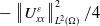 $-\left \| U^\varepsilon _{xx} \right \|_{ L^2 (\Omega )}^2/4$
, we obtain that
$-\left \| U^\varepsilon _{xx} \right \|_{ L^2 (\Omega )}^2/4$
, we obtain that
 \begin{equation} \left \| U^\varepsilon _x \right \|_{ L^2 (\Omega )}^2 (t) \le e^{C_{19}t}\left \| U^\varepsilon _x (\cdot , 0) \right \|_{ L^2 (\Omega )}^2 +\frac {C_{23}}{C_{19}} \big( e^{C_{19} t } -1\big)\varepsilon ^2 = \frac {C_{23}}{C_{19}} \big( e^{C_{19} t } -1\big)\varepsilon ^2 \end{equation}
by the initial condition in (2.17).
Finally, integrating (4.60) over $(0,T)$
, we obtain that
$(0,T)$
, we obtain that
 \begin{equation} \frac 1 2 \left \| U^\varepsilon _{xx} \right \|_{ L^2 (0,T; L^2(\Omega ))}^2 \le \left \| U^\varepsilon _x (\cdot , T)\right \|_{ L^2 (\Omega )}^2 + \frac 1 2 \left \| U^\varepsilon _{xx} \right \|_{ L^2 (0,T; L^2(\Omega ))}^2 \le \varepsilon ^2 C_{23} e^{C_{19} T} T. \end{equation}
Adding (4.61) and (4.62) yields the assertion of this lemma, where we put
 \begin{equation*} C_{16} \,:\!=\, \max \Big \{ \frac {C_{23}}{C_{19}} \big( e^{C_{19} t } -1\big), 2C_{23} e^{C_{19} T} T \Big \}. \end{equation*}
Then, we obtain the following proof.
Proof of Theorem 2.4. Putting
 \begin{align*} C_1 \,:\!=\, \sqrt {2}\big ( C_{11} + C_{11}T + C_{16} \big )^{1/2}, \quad C_2 \,:\!=\, C_1 + \big ( C_9^2 +C_{10}^2 \big )^{1/2} + \sqrt { \frac { T }{2d_j} } \big ( 2d_j C_9^2 + C_9^2 + C_{10}^2 \big )^{1/2}, \end{align*}
where we used Lemma 4.5, Lemma 4.6 for $C_1$
and Lemma 4.4 for
$C_1$
and Lemma 4.4 for $C_2$
. We obtain the convergence of the assertion in this theorem.
$C_2$
. We obtain the convergence of the assertion in this theorem.
Next, we prove Lemma 2.8.
Proof of Lemma 2.8. Set the differences between the solutions and between the kernels as
 \begin{equation*} U(x,t) \,:\!=\, \rho _1(x,t) - \rho _2(x,t), \quad W_{\mbox{e}} (x) \,:\!=\, w_1(x)-w_2(x), \end{equation*}
respectively. The method for this proof is similar to that of Lemmas 4.5 and 4.6. Taking the difference between the equations $(\mbox{P}_1)$
and
$(\mbox{P}_1)$
and $(\mbox{P}_2)$
, we have
$(\mbox{P}_2)$
, we have
 \begin{align} U_t = U_{xx} - ( \rho _1w_{1,x} *U + \rho _1W_{\mbox{e},x}*\rho _2 +Uw_{2,x}*\rho _2 )_x. \end{align}
Multiplying it by $U$
and integrating it over
$U$
and integrating it over $\Omega$
, we have
$\Omega$
, we have
 \begin{align*} \frac {1}{2} \frac {d}{dt} \left \| U \right \|_{ L^2 (\Omega )} ^2 = -\left \| U_x \right \|_{ L^2 (\Omega )} ^2 + \int _{\Omega } ( U_x( \rho _1w_{1,x} *U + \rho _1W_{\mbox{e},x}*\rho _2 +Uw_{2,x}*\rho _2) ) . \end{align*}
Since
 \begin{align*} \int _{\Omega } ( U_x \rho _1w_{1,x} *U ) &\le \left \| \rho _1 \right \|_{ C (\Omega )} \left \| w_{1,x} \right \|_{ L^1 (\Omega )}\left \| U \right \|_{ L^2 (\Omega )} \left \| U_x \right \|_{ L^2 (\Omega )}, \\ \int _{\Omega } ( U_x \rho _1W_{\mbox{e},x}*\rho _2 ) &\le \left \| \rho _1 \right \|_{ C (\Omega )} \left \| W_{\mbox{e}} \right \|_{ L^1 (\Omega )}\left \| \rho _{2,x} \right \|_{ L^2 (\Omega )} \left \| U_x \right \|_{ L^2 (\Omega )},\\ \int _{\Omega } ( U_xUw_{2,x}*\rho _2 ) & \le \left \| \rho _{2} \right \|_{ C (\Omega )} \left \| w_{2,x} \right \|_{ L^1 (\Omega )} \left \| U \right \|_{ L^2 (\Omega )} \left \| U_x \right \|_{ L^2 (\Omega )} , \end{align*}
we can compute that
 \begin{align} \frac {1}{2} \frac {d}{dt} \left \| U \right \|_{ L^2 (\Omega )} ^2 \le -\frac {1}{4} \left \| U_x \right \|_{ L^2 (\Omega )}^2 + \frac {C_{24}}{2} \left \| U \right \|_{ L^2 (\Omega )} ^2 + \frac {C_{25}}{2} \left \| W_{\mbox{e}} \right \|_{ L^1 (\Omega )}^2, \end{align}
where we put
 \begin{align*} C_{24} &\,:\!=\, 2C_{\mbox s}^2\left( \left(C_0^{(1)} \| w_{1,x} \|_{L^1(\Omega )}\right)^2 + \left(C_0^{(2)} \| w_{2,x} \|_{L^1(\Omega )}\right)^2 \right),\\ C_{25} &\,:\!=\, 2 \left(C_{\mbox s}C_0^{(1)}C_0^{(2)}\right)^2, \end{align*}
and $C_{\mbox s}$
is the coefficient from the Sobolev embedding theorem, and
$C_{\mbox s}$
is the coefficient from the Sobolev embedding theorem, and $C_0^{(1)}$
and
$C_0^{(1)}$
and $C_0^{(2)}$
correspond to the constant
$C_0^{(2)}$
correspond to the constant $C_0$
in Proposition 2.1 for
$C_0$
in Proposition 2.1 for $\rho _1$
and
$\rho _1$
and $\rho _2$
, respectively. Applying the Gronwall inequality to this, we have
$\rho _2$
, respectively. Applying the Gronwall inequality to this, we have
 \begin{equation} \left \| U \right \|_{ C([0,T]; L^2 (\Omega ))}^2 \le \frac {C_{25}}{C_{24}} \big(e^{C_{24} T} -1 \big) \left \| W_{\mbox{e}} \right \|_{ L^1 (\Omega )}^2 \,=\!:\,{\tilde C_T^{(1)}} \left \| W_{\mbox{e}} \right \|_{ L^1 (\Omega )}^2. \end{equation}
Integrating (4.64) over $[0,T]$
and adding it and (4.65), we have
$[0,T]$
and adding it and (4.65), we have
 \begin{equation*} \left \| U \right \|_{ C\left([0,T];L^2 (\Omega )\right)}^2 + \left \| U \right \|_{ L^2 (0,T;H^1(\Omega ))}^2 \le {\tilde C_T^{(2)}} \left \| w_1 - w_2 \right \|_{ L^{1} (\Omega )}^2, \quad {\tilde C_T^{(2)}}\,:\!=\, \max \Big \{ {\tilde C_T^{(1)}}, T{\tilde C_T^{(1)}},2C_{25}T e^{C_{24} T} \Big \}. \end{equation*}
Next, multiplying (4.63) by $-U_{xx}$
and integrating it over
$-U_{xx}$
and integrating it over $\Omega$
, we consider the following equation of energy
$\Omega$
, we consider the following equation of energy
 \begin{align*} \frac {1}{2} \frac {d}{dt} \left \| U_{x} \right \|_{ L^2 (\Omega )} ^2 =-\left \| U_{xx}\right \|_{ L^2 (\Omega )} ^2 + \int _{\Omega } ( U_{xx} ( \rho _1w_{1,x} *U + \rho _1W_{\mbox{e},x}*\rho _2 +Uw_{2,x}*\rho _2)_x ). \end{align*}
Since
 \begin{align*} & \int _{\Omega } \left( U_{xx} \left( \rho _{1,x}w_{1,x} *U + \rho _1w_{1,x} *U_{x}\right) \right) \\ &\le \left \| U \right \|_{ C (\Omega )} \left \| w_{1,x} \right \|_{ L^1 (\Omega )} \left \| U_{xx} \right \|_{ L^2 (\Omega )} \left \| \rho _{1,x} \right \|_{ L^2 (\Omega )} + \left \| \rho _1\right \|_{ C (\Omega )} \left \| w_{1,x}\right \|_{ L^1 (\Omega )} \left \| U_{x} \right \|_{ L^2 (\Omega )} \left \| U_{xx} \right \|_{ L^2 (\Omega )}\\ &\le C_{\mbox s} \left \| U \right \|_{ H^1 (\Omega )} \left \| w_{1,x} \right \|_{ L^1 (\Omega )} \left \| U_{xx} \right \|_{ L^2 (\Omega )} \left \| \rho _{1,x} \right \|_{ L^2 (\Omega )} + \left \| \rho _1\right \|_{ C (\Omega )} \left \| w_{1,x}\right \|_{ L^1 (\Omega )} \left \| U_{x} \right \|_{ L^2 (\Omega )} \left \| U_{xx} \right \|_{ L^2 (\Omega )},\\ &\int _{\Omega } \left( U_{xx} \left( \rho _{1,x}W_{\mbox{e},x}*\rho _2 + \rho _1W_{\mbox{e},x}*\rho _{2,x}\right) \right) \\ & \le \left \| \rho _2 \right \|_{ C (\Omega )} \left \| W_{\mbox{e},x} \right \|_{ L^1 (\Omega )} \left \| U_{xx} \right \|_{ L^2 (\Omega )} \left \| \rho _{1,x} \right \|_{ L^2 (\Omega )} + \left \| \rho _1 \right \|_{ C (\Omega )} \left \| W_{\mbox{e},x} \right \|_{ L^1 (\Omega )} \left \| U_{xx} \right \|_{ L^2 (\Omega )} \left \| \rho _{2,x} \right \|_{ L^2 (\Omega )},\\ &\int _{\Omega } \left( U_{xx} \left( U_xw_{2,x}*\rho _2 + U w_{2,x}*\rho _{2,x} \right) \right) \\ &\le \left \| \rho _2 \right \|_{ C (\Omega )} \left \|w_{2,x} \right \|_{ L^1 (\Omega )} \left \| U_x \right \|_{ L^2 (\Omega )} \left \| U_{xx} \right \|_{ L^2 (\Omega )} + C_{\mbox s} \left \| U \right \|_{ H^1 (\Omega )} \left \| \rho _{2,x} \right \|_{ L^2 (\Omega )} \left \|w_{2,x} \right \|_{ L^1 (\Omega )} \left \| U_{xx} \right \|_{ L^2 (\Omega )}, \end{align*}
we can obtain that
 \begin{align} \frac {1}{2} \frac {d}{dt} \left \| U_{x} \right \|_{ L^2 (\Omega )} ^2 &\le -\frac {1}{4} \left \| U_{xx} \right \|_{ L^2 (\Omega )}^2 + \frac {C_{26}}{2} \left \| U \right \|_{ L^2 (\Omega )}^2 + \frac {C_{27}}{2} \left \| U_x \right \|_{ L^2 (\Omega )}^2 + \frac {C_{28}}{2} \left \| W_{\mbox{e},x} \right \|_{ L^1 (\Omega )}^2 \notag \\ &\le -\frac {1}{4} \left \| U_{xx} \right \|_{ L^2 (\Omega )}^2 + \frac {C_{27}}{2} \left \| U_x \right \|_{ L^2 (\Omega )}^2 + \frac {C_{29}}{2} \left \| W_{\mbox{e}} \right \|_{ W^{1,1} (\Omega )}^2 \end{align}
with suitable positive constants from $C_{26}$
to
$C_{26}$
to $C_{29}$
, where we put
$C_{29}$
, where we put
 \begin{align*} C_{26} &\,:\!=\, 4C_{\mbox s}^2 \left( \left( C_0^{(1)} \left \| w_{1,x} \right \|_{ L^1 (\Omega )} \right)^2 + \left( C_0^{(2)} \left \| w_{2,x} \right \|_{ L^1 (\Omega )} \right)^2 \right),\\ &C_{27} \,:\!=\, C_{26} + 4C_{\mbox s}^2\left( \left(C_0^{(1)} \left \| w_{1,x}\right \|_{ L^1 (\Omega )}\right)^2 + \left(C_0^{(2)} \left \| w_{2,x}\right \|_{ L^1 (\Omega )}\right)^2 \right),\\ C_{28} &\,:\!=\, 8\left(C_{\mbox s} C_0^{(1)} C_0^{(2)}\right)^2,\\ C_{29} &\,:\!=\, \max \left\{ \frac {C_{25} C_{26} }{C_{24}} \big(e^{C_{24} T} -1 \big), C_{28} \right\}. \end{align*}
Therefore, the Gronwall inequality yields that
 \begin{equation} \left \| U_x \right \|_{ C\left( [0,T]; L^2 (\Omega )\right)}^2 \le \frac {C_{29}}{C_{27}} (e^{C_{27} T} -1 )\left \| W_{\mbox{e}} \right \|_{ W^{1,1} (\Omega )}^2 \,=\!:\,{\tilde C_T^{(3)}} \left \| W_{\mbox{e}} \right \|_{ W^{1,1} (\Omega )}^2. \end{equation}
Finally integrating (4.64) and (4.66) over $(0,T)$
and adding them and (4.65) and (4.67), we obtain the assertion of Lemma 2.8 by putting
$(0,T)$
and adding them and (4.65) and (4.67), we obtain the assertion of Lemma 2.8 by putting
 \begin{equation*} {\tilde C_T} \,:\!=\, \max \left \{ {\tilde C_T^{(2)}}, {\tilde C_T^{(3)}}, 2C_{29}Te^{C_{27}T} \right\}. \end{equation*}
5. Coefficients of linear sum
We now explain the method used for determining the coefficient $\{ a_j \}_{j=1}^M$
of the linear sum of the fundamental solution for a given even potential function
$\{ a_j \}_{j=1}^M$
of the linear sum of the fundamental solution for a given even potential function $W$
. Furthermore, we will perform the numerical simulations of the approximation of
$W$
. Furthermore, we will perform the numerical simulations of the approximation of $W$
by sum of
$W$
by sum of $\cosh j(L-|x|)$
, and numerical simulations of (P) and (
$\cosh j(L-|x|)$
, and numerical simulations of (P) and ( $\mbox{KS}^{M,\varepsilon }$
) with this series expansion. Since
$\mbox{KS}^{M,\varepsilon }$
) with this series expansion. Since $W$
is even, we only consider
$W$
is even, we only consider $[0,L]$
. Throughout this section, we set
$[0,L]$
. Throughout this section, we set $d_1$
is sufficiently large and
$d_1$
is sufficiently large and $d_j=1/(j-1)^2$
for
$d_j=1/(j-1)^2$
for $j=2,\ldots ,M$
.
$j=2,\ldots ,M$
.
First, we provide the following lemma with respect to the $n$
degree Chebyshev polynomial
$n$
degree Chebyshev polynomial $T_n(x) \,:\!=\, \cos (n\arccos x)$
. We set coefficients as
$T_n(x) \,:\!=\, \cos (n\arccos x)$
. We set coefficients as
 \begin{align*} C^n_k \,:\!=\, (-1)^k 2^{n-2k-1} \frac {n}{n-k} \binom {n-k}{k}, \quad \left(k=0, \cdots , \Big [\frac n 2 \Big ] \right) \end{align*}
for $n \in \mathbb{N}$
, where
$n \in \mathbb{N}$
, where $[\!\cdot\!]$
denotes the Gauss symbol. By this constant, the Chebyshev polynomial of the first kind of
$[\!\cdot\!]$
denotes the Gauss symbol. By this constant, the Chebyshev polynomial of the first kind of $n$
degree
$n$
degree $T_n$
can be expressed as
$T_n$
can be expressed as $T_n(x) = \sum _{k=0}^{[n/2]}C^n_k x^{n-2k}$
for
$T_n(x) = \sum _{k=0}^{[n/2]}C^n_k x^{n-2k}$
for $x\in [-1,1]$
. The properties of the Chebyshev polynomial can be referred from [Reference Mason and Handscomb16] by Mason and Handscomb. Utilising this equation, we have the following Lemma regarding the change of the variable for
$x\in [-1,1]$
. The properties of the Chebyshev polynomial can be referred from [Reference Mason and Handscomb16] by Mason and Handscomb. Utilising this equation, we have the following Lemma regarding the change of the variable for $T_n$
.
$T_n$
.
Lemma 5.1. Setting
 \begin{equation*} \mu ^n_{k,j} \,:\!=\, C^n_k \left( \frac {2}{b-a} \right)^{n-2k} \left( -\frac {b+a}{2} \right)^j \binom {n-2k}{j} \end{equation*}
for $n \in \mathbb{N}$
, we define the coefficient as
$n \in \mathbb{N}$
, we define the coefficient as
 \begin{equation*} \xi ^n_k \,:\!=\, \left \{ \begin{aligned} &\sum _{l=0}^{[n/2]-[(k+1)/2]} \mu ^n_{l,n-2l-k}, \quad \text{if $n$ is even}, \\[4pt] &\sum _{l=0}^{[n/2]-[k/2]} \mu ^n_{l,n-2l-k}, \quad \text{otherwise}. \\ \end{aligned} \right . \end{equation*}
Then,
 \begin{equation*} T_n\left ( \frac {2x - (b+a)}{b-a} \right ) = \sum _{k=0}^n \xi ^n_k x^k, \quad x \in [a,b] \end{equation*}
holds.
Proof of Lemma 5.1. We compute that
 \begin{align*} T_n\left( \frac {2x - (b+a)}{b-a} \right) &= \sum _{k=0}^{[n/2]}C^n_k \left( \frac {2x -(b+a) }{ b-a } \right)^{n-2k} =\sum _{k=0}^{[n/2]}C^n_k \left( \frac {2}{b-a} \right)^{n-2k} \left( x - \frac {b+a}{2}\right)^{n-2k}\\ & = \sum _{k=0}^{[n/2]}C^n_k \left( \frac {2}{b-a} \right)^{n-2k} \sum _{j=0}^{n-2k} \binom {n-2k} { j} x^{n-2k-j} \left( -\frac {b+a}{2} \right)^j\\ & = \sum _{k=0}^{[n/2]} \sum _{j=0}^{n-2k} \mu ^n_{k,j} x^{n-2k-j} = \sum _{k=0}^n \xi ^n_k x^k, \end{align*}
where we used the binomial expansion in the third equality.
Next, we explicitly provide the coefficient of the linear sum of the $n$
degree Lagrange interpolation polynomial with the Chebyshev nodes for the arbitrary function
$n$
degree Lagrange interpolation polynomial with the Chebyshev nodes for the arbitrary function $F=F(x)$
for
$F=F(x)$
for $x\in [a,b]$
. We will replace the arbitrary function
$x\in [a,b]$
. We will replace the arbitrary function $F$
with the function
$F$
with the function $f$
defined in (2.22) to prove Theorem 5.3. The root of the
$f$
defined in (2.22) to prove Theorem 5.3. The root of the $n$
degree Chebyshev polynomial, called Chebyshev nodes, in an arbitrary interval
$n$
degree Chebyshev polynomial, called Chebyshev nodes, in an arbitrary interval $[a,b]$
is given by
$[a,b]$
is given by
 \begin{equation*} r^n_j \,:\!=\, \frac {a+b}{2} + \frac {b-a}{2}\cos \frac {2j+1}{2n}\pi , \quad (j=0,\ldots , n-1). \end{equation*}
We have that
 \begin{equation} \prod _{j=0}^{n}\big(x-r_j^{n+1}\big) =\frac {1}{2^n} \left( \frac {b-a}{2} \right)^{n+1} T_{n+1 }\left( \frac {2x - (b+a)}{b-a} \right), \ n \in \mathbb{N}. \end{equation}
Moreover, setting the coefficient as
 \begin{equation} \zeta ^n_j \,:\!=\, \frac {F\big(r^{n+1}_j\big)}{\prod _{k=0,k\neq j}^n\big(r^{n+1}_j - r^{n+1}_k\big)}, \quad (j=0,\ldots , n) \end{equation}
for $n \in \mathbb{N}$
, we see that the
$n \in \mathbb{N}$
, we see that the $n$
degree Chebyshev polynomial for the function
$n$
degree Chebyshev polynomial for the function $F$
is given by
$F$
is given by
 \begin{equation*} L_n(x)\,:\!=\, \sum _{j=0}^n \zeta ^n_j \prod _{k=0,k\neq j}^n \big(x - r^{n+1}_k\big). \end{equation*}
Note that $L_n( r^{n+1}_j ) = F ( r^{n+1}_j )$
. Then, we obtain the following proposition.
$L_n( r^{n+1}_j ) = F ( r^{n+1}_j )$
. Then, we obtain the following proposition.
Proposition 5.2. Set
 \begin{align} &\beta _{l,j}^{n+1} \,:\!=\, \sum _{k=l}^{n} (r^{n+1}_j)^{k-l} \xi ^{n+1}_{k+1} \quad (l=0,\ldots ,n), \ (j=0,\ldots ,n),\notag \\ b^n_l &\,:\!=\, \frac {1}{2^n} \left( \frac {b-a}{2} \right)^{n+1} \sum _{j=0}^n \zeta ^n_j \beta _{l,j}^{n+1} \quad (l=0,\ldots ,n) \end{align}
for $n \in \mathbb{N}$
. Then, the
$n \in \mathbb{N}$
. Then, the $n$
degree Lagrange interpolation polynomial
$n$
degree Lagrange interpolation polynomial $L_n$
for an arbitrary function
$L_n$
for an arbitrary function $F$
on
$F$
on $[a,b]$
can be described as
$[a,b]$
can be described as
 \begin{equation*} L_n(x)= \sum _{l=0}^n b^n_l x^l, \quad x \in [a,b]. \end{equation*}
Proof of Proposition 5.2. Using Lemma 5.1 and (5.68), we can compute that
 \begin{align*} L_n(x) &=\sum _{j=0}^n \zeta ^n_j \prod _{k=0,k\neq j}^n \big(x - r^{n+1}_k\big)\\ &=\sum _{j=0}^n \zeta ^n_j \frac {1}{2^n} \left( \frac {b-a}{2} \right)^{n+1} T_{n+1 }\left( \frac {2x - (b+a)}{b-a} \right) \frac {1}{x - r^{n+1}_j}\\ &=\frac {1}{2^n} \left( \frac {b-a}{2} \right)^{n+1} \sum _{j=0}^n \zeta ^n_j \frac { \sum _{k=0}^{n+1} \xi ^{n+1}_k x^k}{x - r^{n+1}_j}. \end{align*}
As $x - r^{n+1}_j$
for
$x - r^{n+1}_j$
for $j = 0,\ldots ,n$
are the factors of
$j = 0,\ldots ,n$
are the factors of $T_{n+1}( (2x - (b+a) )/(b-a) )$
, respectively,
$T_{n+1}( (2x - (b+a) )/(b-a) )$
, respectively, $\sum _{k=0}^{n+1} \xi ^{n+1}_k x^k/(x - r^{n+1}_j )$
must be divisible from the factor theorem. Thus, we obtain that
$\sum _{k=0}^{n+1} \xi ^{n+1}_k x^k/(x - r^{n+1}_j )$
must be divisible from the factor theorem. Thus, we obtain that
 \begin{align*} L_n(x) &= \frac {1}{2^n} \left( \frac {b-a}{2} \right)^{n+1} \sum _{j=0}^n\zeta ^n_j \sum _{l=0}^{n} \beta ^{n+1}_{l,j} x^l\\ &=\sum _{l=0}^{n} \left( \frac {1}{2^n} \left( \frac {b-a}{2} \right)^{n+1} \sum _{j=0}^n \zeta ^n_j \beta ^{n+1}_{l,j} \right)x^l = \sum _{l=0}^n b^n_l x^l. \end{align*}
Before the proof of Theorem 5.3, we introduce the following constant for $n \in \mathbb{N}$
and
$n \in \mathbb{N}$
and $j \equiv n\pmod 2$
:
$j \equiv n\pmod 2$
:
 \begin{equation*} \delta ^n_j \,:\!=\, \left \{ \begin{aligned} &\frac {1}{2^{n-1} } \binom n { \frac {n-j}{2} } \quad \text{if $j \neq 0$},\\[4pt] &\frac {1}{2^{ n } } \binom n { \frac {n-j}{2} } \quad \text{if $j=0$}.\\ \end{aligned} \right . \end{equation*}
Using this constant, we can describe the formula as $x^n = \sum _{j=0, j \equiv n\pmod 2}^n \delta ^n_j T_j(x),$
[Reference Mason and Handscomb16]. Differentiating it, we then obtain that
$x^n = \sum _{j=0, j \equiv n\pmod 2}^n \delta ^n_j T_j(x),$
[Reference Mason and Handscomb16]. Differentiating it, we then obtain that $x^n = \sum _{j=0, j \equiv n\pmod 2}^n (j+1)\delta ^{n+1}_{j+1} U_j(x)/(n+1)$
, where
$x^n = \sum _{j=0, j \equiv n\pmod 2}^n (j+1)\delta ^{n+1}_{j+1} U_j(x)/(n+1)$
, where $U_n(x)\,:\!=\, (\sin (n+1)\theta )/\sin \theta , \ (x=\cos \theta )$
is the Chebyshev polynomial of the second kind. In addition, from the induction, we note that
$U_n(x)\,:\!=\, (\sin (n+1)\theta )/\sin \theta , \ (x=\cos \theta )$
is the Chebyshev polynomial of the second kind. In addition, from the induction, we note that $T_n(\!\cosh (L-|x|))= \cosh n(L-|x|)$
for
$T_n(\!\cosh (L-|x|))= \cosh n(L-|x|)$
for $n \in \mathbb{N}$
holds. Using
$n \in \mathbb{N}$
holds. Using $f$
in (2.22) instead of
$f$
in (2.22) instead of $F$
in (5.69), we reconsider the coefficients
$F$
in (5.69), we reconsider the coefficients $\zeta ^n_j$
in (5.69) and
$\zeta ^n_j$
in (5.69) and $b^n_l$
in (5.70) in Theorem 5.3.
$b^n_l$
in (5.70) in Theorem 5.3.
Theorem 5.3.
Assume that $W \in C^m([0,L])$
for given
$W \in C^m([0,L])$
for given $2 \le m \in \mathbb{N}$
and (
2.23
) for
$2 \le m \in \mathbb{N}$
and (
2.23
) for $n \le m-1$
. Let
$n \le m-1$
. Let $\zeta ^n_j$
and
$\zeta ^n_j$
and $b^n_l$
be (
5.69
) with
$b^n_l$
be (
5.69
) with $f$
and (
5.70
) with a natural number
$f$
and (
5.70
) with a natural number $n \le m-1$
for
$n \le m-1$
for $a=1$
and
$a=1$
and $b=\cosh L$
, respectively. Set the coefficient
$b=\cosh L$
, respectively. Set the coefficient $\alpha ^{n}_j$
as
$\alpha ^{n}_j$
as
 \begin{equation*} \alpha ^n_j = \sum _{\substack { k=j \\ k \equiv j \pmod 2}}^n b^n_k\delta ^k_j. \end{equation*}
Then, there exists a constant $C_L$
that is independent of
$C_L$
that is independent of $n$
such that for any
$n$
such that for any $n \le m-1$
 \begin{align*} \left\| W - \sum _{j=0}^{n} \alpha ^{n}_j \cosh j(L-\cdot ) \right\|_{ C^1([0,L])} \le C_L \frac {n+1}{2^{n}n!} \left(\frac {\cosh L-1}{2} \right)^{n} \max _{y\in [1,\cosh L ]}|f^{(n+1)}(y) | \end{align*}
holds.
We note that this theorem can be applicable to the smooth even potential $W$
with (2.23) on
$W$
with (2.23) on $\Omega$
since
$\Omega$
since $\cosh j(L-|x|)$
is even.
$\cosh j(L-|x|)$
is even.
Proof of Theorem 5.3. Recall that $f(y) = W(L- \cosh ^{-1} y)$
. From the property of the Lagrange polynomial for
$f(y) = W(L- \cosh ^{-1} y)$
. From the property of the Lagrange polynomial for $f(y)$
defined in (2.22) for any
$f(y)$
defined in (2.22) for any $y \in [1, \cosh L]$
, there exists a constant
$y \in [1, \cosh L]$
, there exists a constant $\min _i\{ r^{n+1}_i \} \lt c \lt \max _i\{ r^{n+1}_i\}$
such that
$\min _i\{ r^{n+1}_i \} \lt c \lt \max _i\{ r^{n+1}_i\}$
such that
 \begin{equation} f(y) - L_n(y) = \frac { f^{(n+1)}( c ) }{(n+1)!} \prod _{j=1}^{n+1}\big(y-r_j^{n+1}\big) = \frac {f^{(n+1)} ( c ) }{2^n (n+1)!} \left( \frac { b - a }{2} \right)^{n+1} T_{n+1 }\left( \frac {2y - (b+a)}{b-a} \right) \end{equation}
with $b=\cosh L$
and
$b=\cosh L$
and $a=1$
and thus,
$a=1$
and thus,
 \begin{equation*} \frac {1}{2^n(n+1)!} \left(\frac {\cosh L-1}{2} \right)^{n+1} \max _{ y \in [1, \cosh L] }| f^{(n+1)}(y) | \ge \| f - L_n \|_{C([1,\cosh L])}. \end{equation*}
Here, we used $\| T_n \|_{C[0,1]}=1$
because of the definition. Using Proposition 5.2 and changing the variable to
$\| T_n \|_{C[0,1]}=1$
because of the definition. Using Proposition 5.2 and changing the variable to $y = \cosh (L-x)$
for
$y = \cosh (L-x)$
for $x \in [0,L]$
, we can compute the right-hand side of the above inequality as
$x \in [0,L]$
, we can compute the right-hand side of the above inequality as
 \begin{align*} \| f - L_n \|_{C([1,\cosh L])} &= \sup _{y \in [1,\cosh L]} | f(y) - \sum _{j=0}^n b_j^n y^j| = \left\| f - \sum _{j=0}^n b_j^n \sum _{\substack {k=0 \\ k \equiv j\pmod 2}}^j \delta ^j_k T_k\right\|_{C([1,\cosh L])}\\ &=\left\| f(\!\cosh (L-\cdot ) ) - \sum _{j=0}^n b_j^n \sum _{\substack {k=0 \\ k \equiv j\pmod 2}}^j \delta ^j_k T_k(\!\cosh (L-\cdot )) \right\|_{C([0, L])}\\ &=\left\| W - \sum _{j=0}^n b_j^n \sum _{\substack {k=0 \\ k \equiv j\pmod 2}}^j \delta ^j_k \cosh k(L-\cdot ) \right\|_{C([0, L])}\\ &=\left\| W - \sum _{j=0}^n \sum _{\substack {k=j \\ k \equiv j\pmod 2}}^n b_k^n \delta ^k_j \cosh j(L-\cdot ) \right\|_{C([0, L])}\\ &= \left \| W - \sum _{j=0}^n \alpha ^n_j \cosh j(L-\cdot ) \right\|_{C([0, L])}. \end{align*}
Next, differentiating (5.71), we see that
 \begin{align*} f'(y) - L'_n(y) = \frac {f^{(n+1)} ( c ) }{2^n n!} \Big ( \frac { b - a }{2} \Big )^{n} U_{ n }\Big ( \frac {2y - (b+a)}{b-a} \Big ) \end{align*}
because of $T'_{n+1}(x) = (n+1) U_n(x),$
[Reference Mason and Handscomb16]. Setting the function as
$T'_{n+1}(x) = (n+1) U_n(x),$
[Reference Mason and Handscomb16]. Setting the function as $\mathscr{G} = \sqrt {y^2-1}$
for
$\mathscr{G} = \sqrt {y^2-1}$
for $y \in [1,\cosh L]$
, we see that
$y \in [1,\cosh L]$
, we see that $\mathscr{G}(\!\cosh (L-x)) = \sinh (L-x)$
for
$\mathscr{G}(\!\cosh (L-x)) = \sinh (L-x)$
for $x \in [0,L]$
. Then, we can compute that
$x \in [0,L]$
. Then, we can compute that
 \begin{align*} \| \mathscr{G}(f' - L'_n) \|_{C([1,\cosh L])} &=\sup _{y \in [1,\cosh L]} \left| \mathscr{G}(y) \left( f'(y) - \sum _{j=1}^n b_j^n j y^{j-1} \right) \right| \\ &= \left \| \mathscr{G}\left( f' - \sum _{j=1}^n b_j^n \sum _{\substack {k=0 \\ k \equiv j-1\pmod 2}}^{j-1} (k+1) \delta ^j_{k+1} U_k \right) \right\|_{C([1,\cosh L])}\\ &= \left \| W' + \sum _{j=1}^n b_j^n \sum _{\substack {k=1 \\ k \equiv j\pmod 2}}^{j-1} k \delta ^j_{k} \sinh k(L-\cdot ) \right\|_{C([0, L])}\\ &=\left\| W' + \sum _{ j = 1 }^n j \alpha _j^n \sinh j(L-\cdot ) \right \|_{C([0, L])}, \end{align*}
where we used $x^n = \sum _{j=0, j \equiv n\pmod 2}^n (j+1)\delta ^{n+1}_{j+1} U_j(x)/(n+1)$
in the second equality. Thus, we obtain that
$x^n = \sum _{j=0, j \equiv n\pmod 2}^n (j+1)\delta ^{n+1}_{j+1} U_j(x)/(n+1)$
in the second equality. Thus, we obtain that
 \begin{align*} \left\| W' + \sum _{ j = 1 }^n j \alpha _j^n \sinh j(L-\cdot ) \right \|_{C([0, L])} &= \| \mathscr{G} ( f' - L'_n) \|_{C([1,\cosh L])}\\ &\le \sinh L \frac { (n+1) }{2^n n!} \left( \frac { \cosh L - 1 }{2} \right)^{n} \max _{ y \in [1, \cosh L] }| f^{(n+1)} ( y ) |. \end{align*}
Here, we used $\| U_n \|_{C([0,1])} = U_n(0)=n+1$
because the value of
$\| U_n \|_{C([0,1])} = U_n(0)=n+1$
because the value of $(\sin (n+1)\theta )/\sin \theta$
on extreme points in
$(\sin (n+1)\theta )/\sin \theta$
on extreme points in $\theta \in [0,\pi /2]$
is decreasing. Putting
$\theta \in [0,\pi /2]$
is decreasing. Putting $C_L\,:\!=\,\max \{ (\!\cosh L -1)/4, \sinh L \}$
implies the assertion of this theorem.
$C_L\,:\!=\,\max \{ (\!\cosh L -1)/4, \sinh L \}$
implies the assertion of this theorem.
As any continuous function can be approximated by the sum of $(\!\cosh (L-x))^j$
by Theorem 5 in [Reference Ninomiya, Tanaka and Yamamoto19], if the coefficients of
$(\!\cosh (L-x))^j$
by Theorem 5 in [Reference Ninomiya, Tanaka and Yamamoto19], if the coefficients of $(\!\cosh (L-x))^j$
, that is
$(\!\cosh (L-x))^j$
, that is $b^n_j$
, are obtained, it was conceived that the error between
$b^n_j$
, are obtained, it was conceived that the error between $W$
and
$W$
and $\sum _{j=1}^n a_j k_j$
could be estimated. Indeed, the smooth function can be approximated by the Lagrange interpolation polynomial. Thus, it was considered that it should be shown that
$\sum _{j=1}^n a_j k_j$
could be estimated. Indeed, the smooth function can be approximated by the Lagrange interpolation polynomial. Thus, it was considered that it should be shown that $L_n$
can be expressed by the form of
$L_n$
can be expressed by the form of $\sum _{j=0}^n b_j y^j$
. This is generally unknown. However, when the Chebyshev nodes are given to the Lagrange interpolation polynomial, computing
$\sum _{j=0}^n b_j y^j$
. This is generally unknown. However, when the Chebyshev nodes are given to the Lagrange interpolation polynomial, computing $b^n_j$
resulted in the proof since
$b^n_j$
resulted in the proof since $T_n(x) = \sum _{k=0}^{[n/2]}C^n_k x^{n-2k}$
holds and the numerator of the Lagrange polynomial must be divisible by
$T_n(x) = \sum _{k=0}^{[n/2]}C^n_k x^{n-2k}$
holds and the numerator of the Lagrange polynomial must be divisible by $x-r^{n+1}_j$
. In this sense, Proposition 5.2 is essential.
$x-r^{n+1}_j$
. In this sense, Proposition 5.2 is essential.
Next, we prove Corollary 2.6
Proof of Corollary 2.6. Using Theorem 5.3 and $a_j$
defined in (2.27), we can obtain the same estimate as the proof of Theorem 5.3.
$a_j$
defined in (2.27), we can obtain the same estimate as the proof of Theorem 5.3.
Then, we explain the proof of Theorem 2.9.
Proof of Theorem 2.9. According to Theorem 5.3, for any even function $W$
in
$W$
in $C^\infty ([0,L])$
with (2.23) and (2.24) for any
$C^\infty ([0,L])$
with (2.23) and (2.24) for any $n\in \mathbb{N}$
, and arbitrary
$n\in \mathbb{N}$
, and arbitrary $ M\in \mathbb{N}$
, there exist constants
$ M\in \mathbb{N}$
, there exist constants $\{ \alpha _j^{M-1}\}_{j=0}^{M-1}$
such that
$\{ \alpha _j^{M-1}\}_{j=0}^{M-1}$
such that
 \begin{equation*} \left\| W - \sum _{j=0}^{M-1} \alpha _j^{M-1} \cosh j(L-|\cdot |) \right \|_{C^1(\Omega )} \lt C_L \frac { M }{2^{M-1} (M-1)!} \left( \frac {\cosh L -1 }{2} \right)^{M-1} \,=\!:\,C_L C(M). \end{equation*}
Here, we set $n=M-1$
in Theorem 5.3. Putting the parameters as (2.21) and (2.27), then we have
$n=M-1$
in Theorem 5.3. Putting the parameters as (2.21) and (2.27), then we have
 \begin{equation} \left\| W - \sum _{j=1}^M a_j k_j\right\|_{C^1(\Omega )} \lt C_L C(M). \end{equation}
Let $\bar { \rho }(x,t)$
be the solution to (P) with the integral kernel
$\bar { \rho }(x,t)$
be the solution to (P) with the integral kernel $\sum _{j=1}^M a_j k_j$
. Since (5.72) holds and
$\sum _{j=1}^M a_j k_j$
. Since (5.72) holds and $C(M)$
converges to zero as
$C(M)$
converges to zero as $M \to \infty$
, there exists a positive constant
$M \to \infty$
, there exists a positive constant $\delta$
that is independent of
$\delta$
that is independent of $M$
such that
$M$
such that $\|\sum _{j=1}^M a_j k_j\|_{W^{1,1} (\Omega )} \le \delta + \|W \|_{W^{1,1}(\Omega )}$
. Thus, we see that
$\|\sum _{j=1}^M a_j k_j\|_{W^{1,1} (\Omega )} \le \delta + \|W \|_{W^{1,1}(\Omega )}$
. Thus, we see that $\tilde C_T$
in Lemma 2.8 does not depend on
$\tilde C_T$
in Lemma 2.8 does not depend on $M$
. Then, for this fixed
$M$
. Then, for this fixed $M$
, Theorem 2.4 and Lemma 2.8 yield that for any
$M$
, Theorem 2.4 and Lemma 2.8 yield that for any $\varepsilon \gt 0$
 \begin{align*} \left \| \rho - \rho ^{M,\varepsilon } \right \|_{ C( [0,T]; H^1 (\Omega ))} &\le \left \| \rho - \bar { \rho } \right \|_{ C( [0,T]; H^1 (\Omega ))} + \left \| \bar { \rho } - \rho ^{M,\varepsilon } \right \|_{ C( [0,T]; H^1 (\Omega ))} \\ &\le \sqrt { {\tilde C_T} } \left\| W - \sum _{j=1}^M a_j k_j \right\|_{ W^{1,1} (\Omega )} + C_1 \varepsilon \\ &\le 2L C_L \sqrt { {\tilde C_T} } C(M) +C_1 \varepsilon . \end{align*}
Thus, we put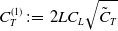 $C_T^{(1)}\,:\!=\, 2L C_L \sqrt { {\tilde C_T} }$
and
$C_T^{(1)}\,:\!=\, 2L C_L \sqrt { {\tilde C_T} }$
and $C_T^{(2)}(M)\,:\!=\, C_1$
, respectively.
$C_T^{(2)}(M)\,:\!=\, C_1$
, respectively.
We performed a numerical simulation of the approximation for the potential $W$
by the linear combination of
$W$
by the linear combination of $\cosh j(L-|x|)$
. The results are shown in Figure 3. The linear combination of
$\cosh j(L-|x|)$
. The results are shown in Figure 3. The linear combination of $\cosh j(L-|x|)$
covers a potential
$\cosh j(L-|x|)$
covers a potential $W$
. The longer the length of the interval
$W$
. The longer the length of the interval $L$
becomes, the worse the rate of convergence becomes from the numerical simulations. However, as the rate of convergence can be exponential as given by Theorem 5.3, the method for determining the coefficient of
$L$
becomes, the worse the rate of convergence becomes from the numerical simulations. However, as the rate of convergence can be exponential as given by Theorem 5.3, the method for determining the coefficient of $a_j$
is compatible with and useful for numerical simulations.
$a_j$
is compatible with and useful for numerical simulations.
Results of a numerical simulation of the approximation for $W$
by the linear combination of
$W$
by the linear combination of $\cosh j(L-|x|)$
. We set
$\cosh j(L-|x|)$
. We set $W(x)=e^{-5x^2}(\cos (3\pi ) x- 1/2 \cos (2\pi x))$
, and
$W(x)=e^{-5x^2}(\cos (3\pi ) x- 1/2 \cos (2\pi x))$
, and $L=2$
. (a) Profiles of
$L=2$
. (a) Profiles of $W$
and the linear sum of
$W$
and the linear sum of $\cosh j(L-|x|)$
. (b) Profiles of
$\cosh j(L-|x|)$
. (b) Profiles of $f$
and the Lagrange interpolation polynomial on
$f$
and the Lagrange interpolation polynomial on $[1, \cosh L]$
. (c) Distribution of
$[1, \cosh L]$
. (c) Distribution of $\{ \alpha ^9_j \}_{j=0}^9$
.
$\{ \alpha ^9_j \}_{j=0}^9$
.
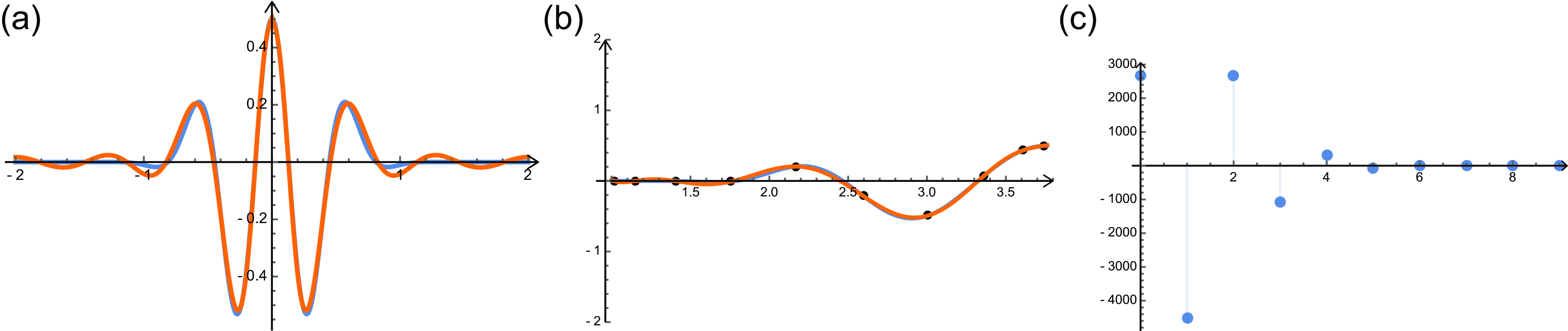
Figures 4 and 8 shows the numerical results of (P) with the potential $W(x)=e^{-5x^2}$
and (
$W(x)=e^{-5x^2}$
and ( $\mbox{KS}^{M,\varepsilon }$
) with parameters
$\mbox{KS}^{M,\varepsilon }$
) with parameters $\varepsilon =0.001$
and
$\varepsilon =0.001$
and $\{\alpha _j^6\}^6_{j=0}$
specified by Theorem 5.3. We can observe that the solution
$\{\alpha _j^6\}^6_{j=0}$
specified by Theorem 5.3. We can observe that the solution $\rho$
in (P) is approximated by that
$\rho$
in (P) is approximated by that $\rho ^{7,\varepsilon }$
in (
$\rho ^{7,\varepsilon }$
in ( $\mbox{KS}^{M,\varepsilon }$
), even though there are seven auxiliary factors
$\mbox{KS}^{M,\varepsilon }$
), even though there are seven auxiliary factors $v_j^{7,\varepsilon }$
. In Figure 4, (c) shows the profiles of both
$v_j^{7,\varepsilon }$
. In Figure 4, (c) shows the profiles of both $W(x)=e^{-5x^2}$
and
$W(x)=e^{-5x^2}$
and $\sum _{j=0}^6 \alpha _j^6 \cosh (j(L-|x|))$
. Since
$\sum _{j=0}^6 \alpha _j^6 \cosh (j(L-|x|))$
. Since $\sum _{j=0}^6 \alpha _j^6 \cosh (j(L-|x|))$
has good accuracy for the approximation of
$\sum _{j=0}^6 \alpha _j^6 \cosh (j(L-|x|))$
has good accuracy for the approximation of $e^{-5x^2}$
, both curves are seen to overlap.
$e^{-5x^2}$
, both curves are seen to overlap.
Results of numerical simulations for (P) with a potential $W(x) = e^{-5x^2}$
and
$W(x) = e^{-5x^2}$
and $\mu$
defined in (
$\mu$
defined in ( $\mbox{P}_\mu$
), and (
$\mbox{P}_\mu$
), and ( $\mbox{KS}^{M,\varepsilon }$
) with
$\mbox{KS}^{M,\varepsilon }$
) with $M=7$
. The parameters are given by
$M=7$
. The parameters are given by $L=1$
,
$L=1$
, $\varepsilon =0.001$
,
$\varepsilon =0.001$
, $d_1=1000000$
,
$d_1=1000000$
, $\mu =5$
and
$\mu =5$
and $d_j$
and
$d_j$
and $a_j$
are provided by (2.21) and (2.27), respectively. (a) Profiles of the numerical result of (P) at
$a_j$
are provided by (2.21) and (2.27), respectively. (a) Profiles of the numerical result of (P) at $t=200.0$
. The horizontal and vertical axes correspond to the position
$t=200.0$
. The horizontal and vertical axes correspond to the position $x$
and
$x$
and $\rho$
, respectively. The red curve is the numerical result of
$\rho$
, respectively. The red curve is the numerical result of $\rho$
. (b) Profiles of the numerical result of (
$\rho$
. (b) Profiles of the numerical result of ( $\mbox{KS}^{M,\varepsilon }$
) at
$\mbox{KS}^{M,\varepsilon }$
) at $t=200.0$
. We impose the same initial data for
$t=200.0$
. We impose the same initial data for $\rho ^{7,\varepsilon }$
as that of
$\rho ^{7,\varepsilon }$
as that of $\rho$
and
$\rho$
and $(v_j)_0= k_j*\rho _0, \ (j=1,\ldots ,M)$
. The axes are set same as that of (a). The red and the other colour curves correspond to
$(v_j)_0= k_j*\rho _0, \ (j=1,\ldots ,M)$
. The axes are set same as that of (a). The red and the other colour curves correspond to $(\rho ^{7,\varepsilon },\{v_j^{7,\varepsilon }\}_{j=1}^7)$
, respectively. (c) Profiles of
$(\rho ^{7,\varepsilon },\{v_j^{7,\varepsilon }\}_{j=1}^7)$
, respectively. (c) Profiles of $W$
and
$W$
and $\sum _{j=0}^6 \alpha _j^6 \cosh (j(L-|x|))$
. The orange dashed and blue curves corresponding to
$\sum _{j=0}^6 \alpha _j^6 \cosh (j(L-|x|))$
. The orange dashed and blue curves corresponding to $W$
and
$W$
and $\sum _{j=0}^6 \alpha _j^6 \cosh (j(L-|x|))$
, respectively, are drawn in a same plane. (d) The distribution of
$\sum _{j=0}^6 \alpha _j^6 \cosh (j(L-|x|))$
, respectively, are drawn in a same plane. (d) The distribution of $\{\alpha _j^6\}_{j=0}^6$
.
$\{\alpha _j^6\}_{j=0}^6$
.
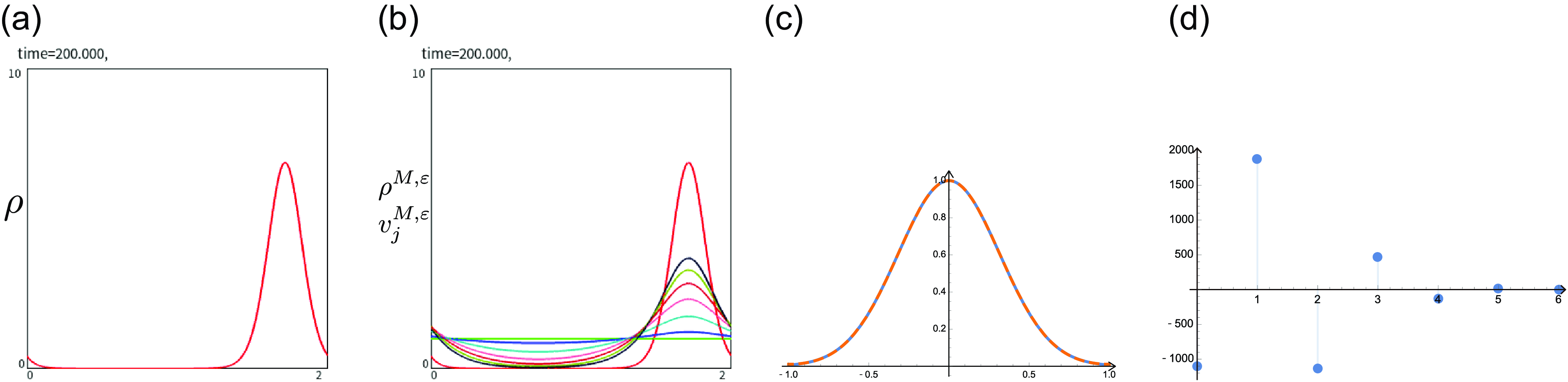
Figure 4 Long description
Panel A: A line graph shows the profile of the numerical result of model (P) at time equals 200. The horizontal axis represents the position x, and the vertical axis represents the density ρ. The red curve indicates the numerical result of ρ. Panel B: A line graph displays the profiles of the numerical result of model (KS^M,ε) at time equals 200. The horizontal and vertical axes are the same as in Panel A. The red curve and other colored curves correspond to (ρ^7,ε) and (v_j^7,ε) for j equals 1 to 7, respectively. Panel C: A line graph shows the profiles of the potential W(x) and the sum of α_j^6 cosh(j(L-|x|)) for j equals 0 to 6. The orange dashed curve represents W, and the blue curve represents the sum of α_j^6 cosh(j(L-|x|)). Panel D: A scatter plot illustrates the distribution of α_j^6 for j equals 0 to 6.
6. Linear stability analysis
In this section, we perform a linear stability analysis around the equilibrium point for (P) and ( $\mbox{KS}^{M,\varepsilon }$
) with three components to specify the role of advective nonlocal interactions in pattern formations. We demonstrate that the eigenvalue of the linearised operator of (
$\mbox{KS}^{M,\varepsilon }$
) with three components to specify the role of advective nonlocal interactions in pattern formations. We demonstrate that the eigenvalue of the linearised operator of ( $\mbox{KS}^{M,\varepsilon }$
) converges to that of (P) as
$\mbox{KS}^{M,\varepsilon }$
) converges to that of (P) as $\varepsilon \to 0$
when the integral kernel is given by
$\varepsilon \to 0$
when the integral kernel is given by $k_j$
of (2.4). We analyse the following equation with the parameter
$k_j$
of (2.4). We analyse the following equation with the parameter $\mu \gt 0$
:
$\mu \gt 0$
:
 \begin{equation*} \qquad\qquad\qquad\qquad\qquad\qquad\rho _ t = \rho _{ xx } - \mu ( \rho ( W*\rho )_x )_x \ \text{in} \ \Omega \times (0,\infty ). \qquad\qquad\qquad\qquad\qquad (\mbox{P}_\mu)\end{equation*}
We explain the instability of the solution near the equilibrium point. Let $\rho ^*\gt 0$
and
$\rho ^*\gt 0$
and $ \xi =\xi (x,t)$
be an arbitrary constant and a small perturbation, respectively.
$ \xi =\xi (x,t)$
be an arbitrary constant and a small perturbation, respectively. $\rho = \rho ^*$
becomes a constant stationary solution of (P). Putting
$\rho = \rho ^*$
becomes a constant stationary solution of (P). Putting $\rho (x,t) = \rho ^* + \xi (x,t)$
and substituting it for (
$\rho (x,t) = \rho ^* + \xi (x,t)$
and substituting it for ( $\mbox{P}_\mu$
), we have
$\mbox{P}_\mu$
), we have
 \begin{align*} \xi _t & = \xi _{xx} - \mu \left( (\xi + \rho ^*) W * (\xi + \rho ^*)_x \right)_x = \xi _{xx} - \mu ( \rho ^* W*\xi _{xx} + \xi _xW*\xi _x + \xi W*\xi _{xx}). \end{align*}
Focusing on the linear part of above, we denote the linear operator $\mathscr L$
by
$\mathscr L$
by
 \begin{equation*} \mathscr{L}[u]\,:\!=\, u_{xx} - \mu \rho ^* W*u_{xx}. \end{equation*}
Because this linearised operator has $\mu \rho ^*$
, the effects of the strength of aggregation and the mass volume on the pattern formation around the constant stationary solution are equivalent. Therefore, we replace
$\mu \rho ^*$
, the effects of the strength of aggregation and the mass volume on the pattern formation around the constant stationary solution are equivalent. Therefore, we replace $ \mu \rho ^*$
with
$ \mu \rho ^*$
with $\mu$
. Defining the Fourier coefficient of
$\mu$
. Defining the Fourier coefficient of $W$
as
$W$
as
 \begin{equation*} \omega _n \,:\!=\, \frac {1}{ \sqrt {2L} }\int _\Omega W(x) e^{-i\sigma _n x} dx, \quad n \in \mathbb{Z}, \end{equation*}
we have the following lemma with respect to the eigenvalues and eigenfunctions:
Lemma 6.1. Setting the eigenvalues
 \begin{equation*} \lambda ( n ) = -\sigma _n^2( 1 - \sqrt {2L} \mu \omega _n), \end{equation*}
then we have
 \begin{equation*} \mathscr L[ e^{i \sigma _n x } ] = \lambda ( n ) e^{i \sigma _n x }, \quad n \in \mathbb{Z}. \end{equation*}
Proof. The proof follows from a direct calculation
 \begin{align*} &(e^{ i \sigma _n x })_{xx} = -\sigma _n^2 e^{i \sigma _n x }, \\ &W*(e^{ i \sigma _n \cdot })_{xx} = -\sigma _n^2 \int _\Omega W(y) e^{i \sigma _n (x-y) } dy= - \sqrt {2L} \sigma _n^2 \omega _n e^{i \sigma _n x }. \end{align*}
Using this lemma, we find the solution to $\xi _t = \mathscr L [\xi ]$
around
$\xi _t = \mathscr L [\xi ]$
around $\rho ^*$
in the form of
$\rho ^*$
in the form of $ \sum _{n\in \mathbb{Z}} \hat {\xi }_n e^{\lambda _n t} e^{i \sigma _n x }$
, where
$ \sum _{n\in \mathbb{Z}} \hat {\xi }_n e^{\lambda _n t} e^{i \sigma _n x }$
, where $\{ \hat {\xi }_n \}$
is the Fourier coefficient.
$\{ \hat {\xi }_n \}$
is the Fourier coefficient.
Results of a numerical simulation for ( $\mbox{P}_\mu$
) with (2.6). The parameters are
$\mbox{P}_\mu$
) with (2.6). The parameters are $\mu =5.0$
,
$\mu =5.0$
, $d_1=0.1$
and
$d_1=0.1$
and $d_2=3.0$
, and the initial data are given by
$d_2=3.0$
, and the initial data are given by $1.0$
with small perturbations. The horizontal and vertical axes correspond to the position
$1.0$
with small perturbations. The horizontal and vertical axes correspond to the position $x$
and value of solution
$x$
and value of solution $\rho$
, respectively. The red curve corresponds to the solution
$\rho$
, respectively. The red curve corresponds to the solution $\rho$
. The left, middle left, middle right and right pictures exhibit the profiles of solutions of (
$\rho$
. The left, middle left, middle right and right pictures exhibit the profiles of solutions of ( $\mbox{P}_\mu$
) with (2.6) in the interval
$\mbox{P}_\mu$
) with (2.6) in the interval $[0, 10]$
at
$[0, 10]$
at $t = 0, 0.5, 1.0$
and
$t = 0, 0.5, 1.0$
and $3.0$
, respectively.
$3.0$
, respectively.
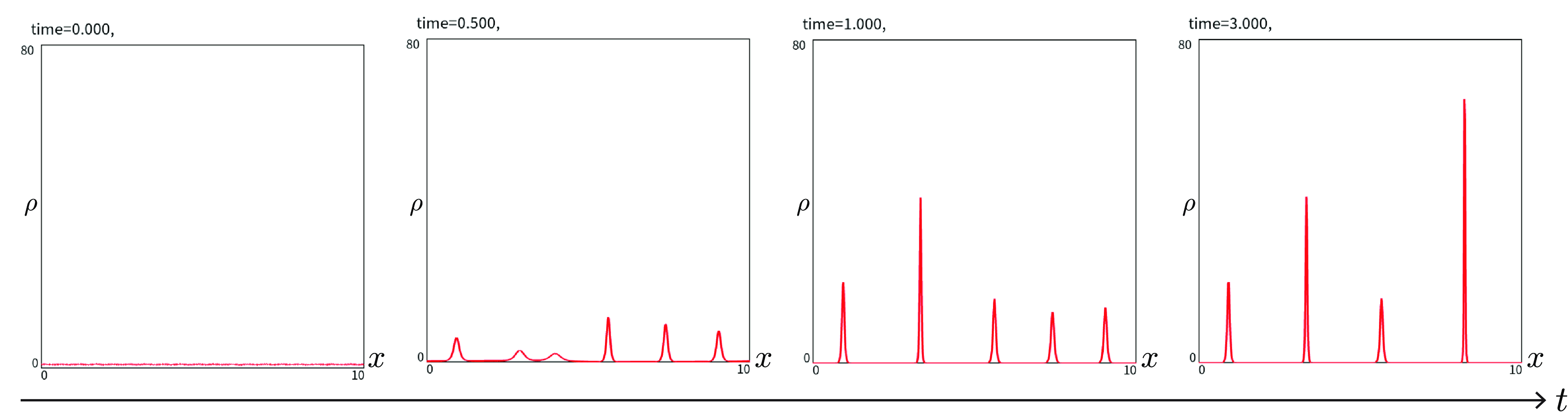
Results of a numerical simulation for ( $\mbox{P}_\mu$
) with (2.7). The parameters are
$\mbox{P}_\mu$
) with (2.7). The parameters are $\mu =4.0$
and
$\mu =4.0$
and $R=1.0$
, and the initial data are given by
$R=1.0$
, and the initial data are given by $1.0$
with small perturbations. The horizontal and vertical axes correspond to the position
$1.0$
with small perturbations. The horizontal and vertical axes correspond to the position $x$
and value of solution
$x$
and value of solution $\rho$
, respectively. The red curve corresponds to the solution
$\rho$
, respectively. The red curve corresponds to the solution $\rho$
. The left, middle left, middle right and right pictures exhibit the profiles of solutions of (
$\rho$
. The left, middle left, middle right and right pictures exhibit the profiles of solutions of ( $\mbox{P}_\mu$
) with (2.7) in the interval
$\mbox{P}_\mu$
) with (2.7) in the interval $[0, 10]$
at
$[0, 10]$
at $t = 0, 0.8, 2.0$
and
$t = 0, 0.8, 2.0$
and $12.0$
, respectively.
$12.0$
, respectively.
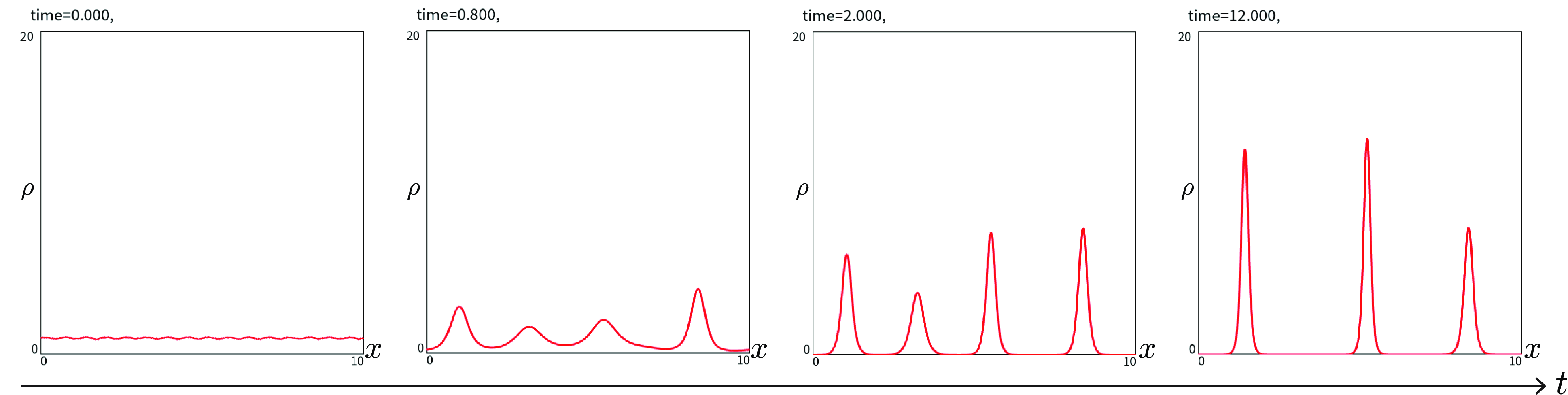
Here, we recall the concept of the diffusion-driven instability in pattern formations proposed by Turing [Reference Turing21]. Diffusion-driven instability is a paradox where diffusion, typically leading to concentration homogenisation, destabilises the uniform stationary solution and induces nonuniformity due to the difference in the diffusion coefficients. By using the eigenvalue $\lambda =\lambda (n)$
for the linear operator of the reaction-diffusion system, the diffusion-driven instability can be defined as the eigenvalue
$\lambda =\lambda (n)$
for the linear operator of the reaction-diffusion system, the diffusion-driven instability can be defined as the eigenvalue $\lambda$
satisfies
$\lambda$
satisfies $\lambda (0)\lt 0$
and there exists
$\lambda (0)\lt 0$
and there exists $n\in \mathbb{Z}$
such that
$n\in \mathbb{Z}$
such that $\lambda (n)\gt 0$
. For the model (
$\lambda (n)\gt 0$
. For the model ( $\mbox{P}_\mu$
), the similar situation occurs. If
$\mbox{P}_\mu$
), the similar situation occurs. If $W$
satisfies that
$W$
satisfies that $\lim _{n \to \pm \infty } \omega _n=0$
and that there exists
$\lim _{n \to \pm \infty } \omega _n=0$
and that there exists $0 \neq n_1 \in \mathbb{N}$
such that
$0 \neq n_1 \in \mathbb{N}$
such that ${\displaystyle } Re \omega _{n_1} \gt 0$
, the maximum eigenvalue may be attained around
${\displaystyle } Re \omega _{n_1} \gt 0$
, the maximum eigenvalue may be attained around $n=n_1$
. In that case, the unstable mode around a stable equilibrium point is given by
$n=n_1$
. In that case, the unstable mode around a stable equilibrium point is given by $e^{i \sigma _{n_1} x }$
.
$e^{i \sigma _{n_1} x }$
.
We performed numerical simulations of ( $\mbox{P}_\mu$
) with the integral kernel (2.6) and (2.7) with the finite volume method. Figures 5 and 6 present the results. The Fourier coefficients for the integral kernels (2.6) and (2.7) are given by
$\mbox{P}_\mu$
) with the integral kernel (2.6) and (2.7) with the finite volume method. Figures 5 and 6 present the results. The Fourier coefficients for the integral kernels (2.6) and (2.7) are given by
 \begin{align*} &\omega _{n,1} = \frac {1}{\sqrt {2 L}} \left (\frac { 1 }{d_1 \sigma _n^2+1} - \frac { 1 }{d_2 \sigma _n^2 +1}\right ), \\[4pt] &\omega _{n,2} = \frac {\sqrt {2} }{ \sqrt { L} } \frac { 1}{ \sigma _n^2 } \left(1-\cos (R_0 \sigma _n ) \right), \end{align*}
respectively. Figures 1 (b) and 2 (b) show the distributions of the eigenvalues with $\omega _{n,1}$
and
$\omega _{n,1}$
and $\omega _{n,2}$
. The number of peaks of the solution at the beginning of the pattern formation corresponds to the maximum wave number in Figures 5 and 6, respectively.
$\omega _{n,2}$
. The number of peaks of the solution at the beginning of the pattern formation corresponds to the maximum wave number in Figures 5 and 6, respectively.
For (2.6), by introducing $v^\varepsilon _1=k_1*\rho$
and
$v^\varepsilon _1=k_1*\rho$
and $v^\varepsilon _2=k_2*\rho$
into
$v^\varepsilon _2=k_2*\rho$
into $W$
, the solution of (
$W$
, the solution of ( $\mbox{P}_\mu$
) can be approximated by that of the 3-component Keller–Segel system from Theorem 2.4:
$\mbox{P}_\mu$
) can be approximated by that of the 3-component Keller–Segel system from Theorem 2.4:
 \begin{equation} \left \{ \begin{aligned} \rho ^{\varepsilon }_ t & = ( \rho ^{\varepsilon })_{xx} - \mu \big ( \rho ^{\varepsilon } ( v_1^\varepsilon - v_2^\varepsilon )_x \big )_x,\\ (v_1^\varepsilon )_t &= \frac {1}{\varepsilon } \big ( d_1 ( v_1^\varepsilon )_{xx} - v_1^\varepsilon + \rho ^{\varepsilon } \big ),\\ (v_2^\varepsilon )_t &= \frac {1}{\varepsilon } \big ( d_2 ( v_{2}^\varepsilon ) _{xx} - v_2^\varepsilon + \rho ^{\varepsilon } \big ) \end{aligned} \right .\ \text{in} \ \Omega \times (0,\infty ) \end{equation}
with $0 \lt \varepsilon \ll 1$
. In (6.73),
$0 \lt \varepsilon \ll 1$
. In (6.73), $v_1^\varepsilon$
and
$v_1^\varepsilon$
and $v_2^\varepsilon$
represent the attractive and repulsive substances in chemotactic process, respectively. By determining the solution as a Fourier series expansion, the linearised problem is provided by the following system:
$v_2^\varepsilon$
represent the attractive and repulsive substances in chemotactic process, respectively. By determining the solution as a Fourier series expansion, the linearised problem is provided by the following system:
 \begin{equation*} \boldsymbol{\varphi }_t = \begin{pmatrix} -\sigma _n^2 & \mu \sigma _n^2 & - \mu \sigma _n^2 \\[6pt] \dfrac {1}{\varepsilon } & \dfrac {-d_1 \sigma _n^2 -1 }{\varepsilon } & 0\\[6pt] \dfrac {1}{\varepsilon } & 0 & \dfrac {-d_2 \sigma _n^2 -1 }{\varepsilon } \end{pmatrix} \boldsymbol{\varphi }, \quad \boldsymbol{\varphi } \,:\!=\, \begin{pmatrix} (\hat {\varphi _1})_n\\[2mm] (\hat {\varphi _2})_n\\[2mm] (\hat {\varphi _3})_n \end{pmatrix}, \end{equation*}
where $(\hat {\varphi _3})_n$
is the Fourier coefficient for the perturbations of
$(\hat {\varphi _3})_n$
is the Fourier coefficient for the perturbations of $v_2^\varepsilon$
. The characteristic polynomial is given by
$v_2^\varepsilon$
. The characteristic polynomial is given by
 \begin{align*} P_2(\lambda ,\varepsilon )&= -\lambda ^3 - \Big ( C_{31} + \frac { C_{33} }{ \varepsilon } \Big ) \lambda ^2 - \Big ( \frac { C_{34} }{\varepsilon ^2} +\frac { C_{35} }{\varepsilon } \Big )\lambda - \frac { C_{36} }{\varepsilon ^2},\\ C_{33}&\,:\!=\, 2+d_1\sigma _n^2+d_2\sigma _n^2,\\ C_{34}&\,:\!=\, \left(1+d_1\sigma _n^2\right)\left(1+d_2\sigma _n^2 \right),\\ C_{35}&\,:\!=\,\sigma _n^2\left( 2+ d_1\sigma _n^2 + d_2\sigma _n^2 \right),\\ C_{36}&\,:\!=\,\sigma _n^2\left(1+d_1\sigma _n^2\right)\left(1+d_2\sigma _n^2 \right) + \mu \left( d_1 -d_2 \right)\sigma _n^4. \end{align*}
Then, we can see that
 \begin{align*} \varepsilon ^2\frac {\partial P_2}{\partial \lambda } &= -3\varepsilon ^2\lambda ^2 -2\varepsilon ( \varepsilon C_{31} + C_{33} ) \lambda -( C_{34} +\varepsilon C_{35}) \\ &\to - (1+d_1\sigma _n^2)(1+d_2\sigma _n^2 ) \lt 0 \quad (\varepsilon \to 0+0). \end{align*}
Only one eigenvalue converges to a bounded value when $\varepsilon \to 0+0$
from the implicit function theorem. Setting the eigenvalue as
$\varepsilon \to 0+0$
from the implicit function theorem. Setting the eigenvalue as $\lambda _\varepsilon$
, we can solve that
$\lambda _\varepsilon$
, we can solve that
 \begin{equation*} \lim _{\varepsilon \to 0+0}\varepsilon ^2 P_2(\lambda _\varepsilon ,\varepsilon ) = - C_{34} \lambda _0 - C_{36} =0, \end{equation*}
and thus
 \begin{equation*} \lambda _{0} = -\sigma _n^2 + \frac { \mu ( d_2 -d_1 )\sigma _n^4 }{ \left(1+d_1\sigma _n^2\right)\left(1+d_2\sigma _n^2 \right) } = -\sigma _n^2\left( 1- \mu \sqrt {2L} \omega _{n,1} \right). \end{equation*}
This implies that the solution to (6.73) and ( $\mbox{P}_\mu$
) with (2.6) are sufficiently close, but also that the Fourier mode of (
$\mbox{P}_\mu$
) with (2.6) are sufficiently close, but also that the Fourier mode of ( $\mbox{P}_\mu$
) when the pattern forms around an equilibrium point is also extremely close to that of the 3-component attraction-repulsion Keller–Segel system (6.73). Because the constant stationary solution is destabilised by the auxiliary factors
$\mbox{P}_\mu$
) when the pattern forms around an equilibrium point is also extremely close to that of the 3-component attraction-repulsion Keller–Segel system (6.73). Because the constant stationary solution is destabilised by the auxiliary factors $v_1^\varepsilon$
and
$v_1^\varepsilon$
and $v_2^\varepsilon$
, the mechanism of the pattern formation is almost the same as that of diffusion-driven instability. In other words, if the integral kernel is provided by (2.6), the solution to (P) is sufficiently close to that of the Keller–Segel system, which can cause the diffusion-driven instability, and thereby suggesting that the kernel
$v_2^\varepsilon$
, the mechanism of the pattern formation is almost the same as that of diffusion-driven instability. In other words, if the integral kernel is provided by (2.6), the solution to (P) is sufficiently close to that of the Keller–Segel system, which can cause the diffusion-driven instability, and thereby suggesting that the kernel $W$
is crucial in generating the diffusion-driven instability in the nonlocal Fokker–Planck equation (P) in linear sense.
$W$
is crucial in generating the diffusion-driven instability in the nonlocal Fokker–Planck equation (P) in linear sense.
We performed a numerical simulation of (6.73) with $\varepsilon =0.001$
. The profile of the solution
$\varepsilon =0.001$
. The profile of the solution $\rho ^\varepsilon$
at each time point in Figure 7 is similar to that of
$\rho ^\varepsilon$
at each time point in Figure 7 is similar to that of $\rho$
in Figure 5. These figures also indicate that stationary solutions to (P) may be approximated by those to (
$\rho$
in Figure 5. These figures also indicate that stationary solutions to (P) may be approximated by those to ( $\mbox{KS}^{M,\varepsilon }$
). As explained above, by approximating the dynamics of nonlocal evolution equations using Keller–Segel systems, we can describe the nonlocal dynamics within the framework of local dynamics and identify both mechanisms.
$\mbox{KS}^{M,\varepsilon }$
). As explained above, by approximating the dynamics of nonlocal evolution equations using Keller–Segel systems, we can describe the nonlocal dynamics within the framework of local dynamics and identify both mechanisms.
The results of a numerical simulation for (6.73). The parameters $\mu , d_1, d_2$
and the initial data are same as that in Figure 5, and
$\mu , d_1, d_2$
and the initial data are same as that in Figure 5, and $\varepsilon =0.001$
and
$\varepsilon =0.001$
and $((v_1)_0,(v_2)_0)=( k_1*\rho _0, k_2*\rho _0 )$
. The horizontal and vertical axes correspond to the position
$((v_1)_0,(v_2)_0)=( k_1*\rho _0, k_2*\rho _0 )$
. The horizontal and vertical axes correspond to the position $x$
and value of solutions
$x$
and value of solutions $\rho ^\varepsilon$
,
$\rho ^\varepsilon$
, $v_1^\varepsilon$
and
$v_1^\varepsilon$
and $v_2^\varepsilon$
, respectively. The red, green and blue curves correspond to the solution
$v_2^\varepsilon$
, respectively. The red, green and blue curves correspond to the solution $\rho ^\varepsilon$
,
$\rho ^\varepsilon$
, $v_1^\varepsilon$
and
$v_1^\varepsilon$
and $v_2^\varepsilon$
, respectively. The left, middle left, middle right and right pictures exhibit the profiles of solutions of (6.73) in the interval
$v_2^\varepsilon$
, respectively. The left, middle left, middle right and right pictures exhibit the profiles of solutions of (6.73) in the interval $[0, 10]$
at
$[0, 10]$
at $t = 0, 0.5, 1.0$
and
$t = 0, 0.5, 1.0$
and $3.0$
, respectively.
$3.0$
, respectively.
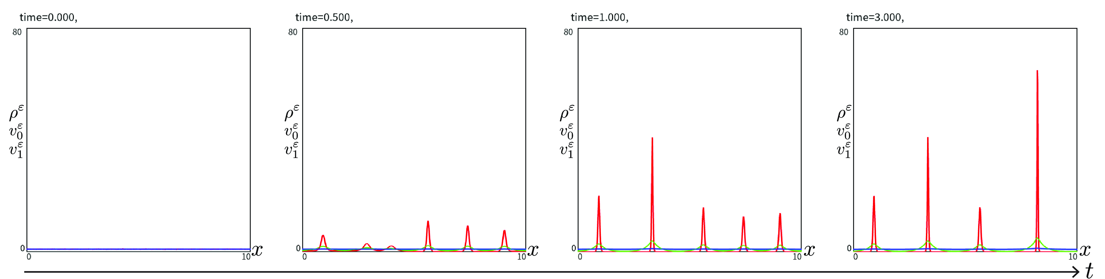
Comparison of the time evolutions of numerical results given in Figure 4 (a) and (b) until $t=1.0$
.
$t=1.0$
.
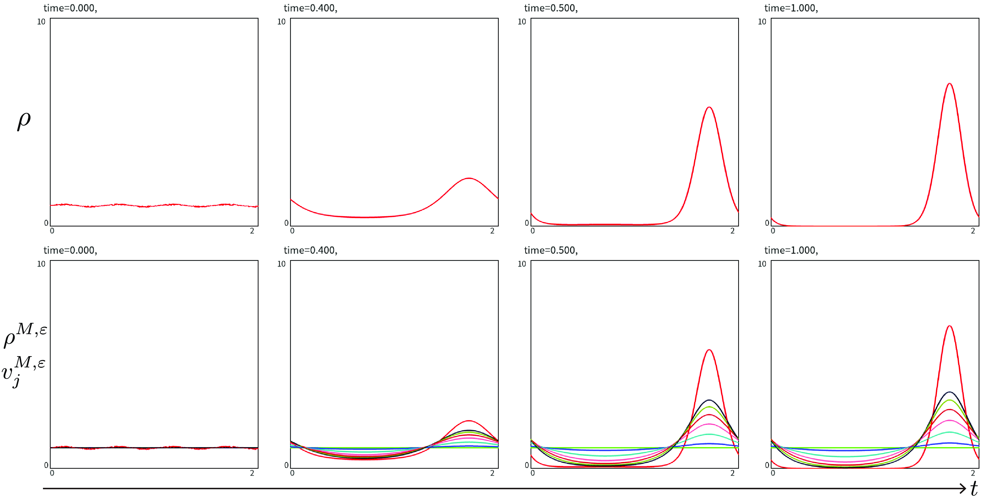
Figure 8 Long description
The image contains eight line graphs arranged in two rows and four columns. Each graph shows the evolution of variables over time. Panel A: The top row contains four line graphs labeled with different time points: 0.000, 0.400, 0.500, and 1.000. The y-axis is labeled with the Greek letter rho (ρ) and ranges from 0 to 10. The x-axis is labeled with the Greek letter xi (ξ) and ranges from 0 to 2. The graphs show the evolution of the density variable ρ over time. At time 0.000, the graph is relatively flat with minor fluctuations. As time progresses to 0.400, 0.500, and 1.000, a distinct peak forms and becomes more pronounced. Panel B: The bottom row contains four line graphs labeled with the same time points as the top row. The y-axis is labeled with ρᵐ,ε and vⱼᵐ,ε, and ranges from 0 to 10. The x-axis is labeled with the Greek letter xi (ξ) and ranges from 0 to 2. These graphs show the evolution of multiple variables, indicated by different colored lines. Initially, at time 0.000, the lines are relatively flat. As time progresses to 0.400, 0.500, and 1.000, the lines form peaks and troughs, indicating the interaction of multiple variables over time.
7. Concluding remarks
We approximated the solutions of the nonlocal Fokker–Planck equation with any even advective nonlocal interactions (P) by those of multiple components of the Keller–Segel system ( $\mbox{KS}^{M,\varepsilon }$
). This indicates that the mechanism of the weight function for determining the velocity by sensing the density globally in space can be realised by combining multiple chemotactic factors. Additionally, our results show that this diffusion–aggregation process can be described as a chemotactic process. We propose a method in which the parameters
$\mbox{KS}^{M,\varepsilon }$
). This indicates that the mechanism of the weight function for determining the velocity by sensing the density globally in space can be realised by combining multiple chemotactic factors. Additionally, our results show that this diffusion–aggregation process can be described as a chemotactic process. We propose a method in which the parameters $\{d_j, a_j\}$
can be determined based on the profile of the potential
$\{d_j, a_j\}$
can be determined based on the profile of the potential $W$
. Using the Keller–Segel type approximation, we rigorously demonstrate that the destabilisation of the solution near equilibrium points in the nonlocal Fokker–Planck equation closely resembles diffusion-driven instability. This type of analysis can be applied to other nonlocal evolution equations with advective nonlocal interactions, such as cell adhesion models.
$W$
. Using the Keller–Segel type approximation, we rigorously demonstrate that the destabilisation of the solution near equilibrium points in the nonlocal Fokker–Planck equation closely resembles diffusion-driven instability. This type of analysis can be applied to other nonlocal evolution equations with advective nonlocal interactions, such as cell adhesion models.
The Keller–Segel approximation also benefits the numerical algorithm in (P). By approximating the potential $W$
by
$W$
by $\sum _{j=1}^Ma_j k_j$
using Theorem 5.3 and solving (
$\sum _{j=1}^Ma_j k_j$
using Theorem 5.3 and solving ( $\mbox{KS}^{M,\varepsilon }$
) or
$\mbox{KS}^{M,\varepsilon }$
) or $({\rm{KS}}^{M,0})$
numerically, we can remove the nonlocality from (P). By calculating these local systems instead of (P) using a simple integral scheme, a numerical simulation can be performed more rapidly. Indeed, the calculation cost as performed in Figures 4 (b) and 7 is
$({\rm{KS}}^{M,0})$
numerically, we can remove the nonlocality from (P). By calculating these local systems instead of (P) using a simple integral scheme, a numerical simulation can be performed more rapidly. Indeed, the calculation cost as performed in Figures 4 (b) and 7 is $O(MN)$
in the time loop iteration, where
$O(MN)$
in the time loop iteration, where $O$
is the Landau symbol and
$O$
is the Landau symbol and $N$
is the number of the spatial mesh. Here, we used the finite volume method and LU decomposition with a tridiagonal matrix.
$N$
is the number of the spatial mesh. Here, we used the finite volume method and LU decomposition with a tridiagonal matrix.
Theorem 2.9 indicates that local dynamics, such as the Keller–Segel system, and nonlocal dynamics, such as the nonlocal Fokker–Planck equation, can be bridged in the sense of continuous evolutionary behaviour. Thus, we can treat the problem (P) within the framework of ( $\mbox{KS}^{M,\varepsilon }$
) if (
$\mbox{KS}^{M,\varepsilon }$
) if ( $\mbox{KS}^{M,\varepsilon }$
) is easier. As demonstrated by the linear stability analysis of (
$\mbox{KS}^{M,\varepsilon }$
) is easier. As demonstrated by the linear stability analysis of ( $\mbox{KS}^{M,\varepsilon }$
), we can characterise the solutions to (P) for local dynamics.
$\mbox{KS}^{M,\varepsilon }$
), we can characterise the solutions to (P) for local dynamics.
According to Ninomiya et al. [Reference Ninomiya, Tanaka and Yamamoto19], the existence of parameters $\{ a_j\}$
was shown for the continuous integral kernel
$\{ a_j\}$
was shown for the continuous integral kernel $W$
although the explicit formula of the coefficients
$W$
although the explicit formula of the coefficients $\{ a_j\}$
was not obtained. This suggests that the condition of Theorem 5.3 for determining
$\{ a_j\}$
was not obtained. This suggests that the condition of Theorem 5.3 for determining $\{ a_j\}$
for potential
$\{ a_j\}$
for potential $W$
may be relaxed. We aim to intensify this investigation in the future.
$W$
may be relaxed. We aim to intensify this investigation in the future.
Financial support
The authors were partially supported by JSPS KAKENHI Grant Number 22K03444 and 24H00188. HM was partially supported by JSPS KAKENHI Grant Number 21KK0044 and by the Joint Research Center for Science and Technology of Ryukoku University. YT was partially supported by JSPS KAKENHI Grant Number 20K14364 and 24K06848 and by Special Research Expenses of Future University Hakodate. A visualisation software, GLSC3D, was used to visualise numerical solutions.
Competing interests
The authors declare that they have no conflict of interest.
Data availability statement
The source codes used to produce the numerical solutions in this manuscript are available on Zenodo at link: https://zenodo.org/records/15583545.
Appendix A. Proof of Lemma 3.4
Proof. First, we denote the Fourier coefficients of $f$
and
$f$
and $g$
by
$g$
by
 \begin{equation*} f_n\,:\!=\, \frac {1}{\sqrt {2L}}\int _\Omega f(x) e^{-i\sigma _n x} dx, \quad g_n(t)\,:\!=\, \frac {1}{\sqrt {2L}}\int _\Omega g(x,t) e^{-i\sigma _n x} dx, \end{equation*}
for $n \in \mathbb{Z}$
, respectively.
$n \in \mathbb{Z}$
, respectively.
Then, using the orthogonality and the Parseval identity, we compute that
 \begin{align*} \left \| G * f \right \| _{ L^2 (\Omega )} ^2 (t) &= \left \| \frac {1}{\sqrt {2L}} \sum _{n \in \mathbb{Z}} e^{- \sigma _n^2 t} e^{i \sigma _n \cdot } f_n \right \|_{ L^2 (\Omega )} ^2 = \sum _{n \in \mathbb{Z}} e^{- 2 \sigma _n^2 t} f_n^2 \le \sum _{n \in \mathbb{Z}} f_n^2 = \left \| f \right \|_{ L^2 (\Omega )}^2. \end{align*}
Straightforwardly, we can calculate that
 \begin{align*} \left \| \int _0^t \int _\Omega G( \cdot -y , t-s) g (y,s) dy ds \right \| _{ L^2 (\Omega )}^2 &= \left \| \frac {1}{\sqrt {2L}} \sum _{n \in \mathbb{Z}} e^{ -\sigma _n^2 t} e^{i \sigma _n \cdot } \int _0^t e^{\sigma _n^2 s} g_n(s) ds \right \|_{ L^2 (\Omega )} ^2 \nonumber \\[5pt] & = \sum _{n \in \mathbb{Z}} e^{ - 2 \sigma _n^2 t} \left( \int _0^t e^{\sigma _n^2 s} g_n(s) ds \right)^2 \nonumber \\[5pt] & \le \sum _{n \in \mathbb{Z}} \frac {1}{\sigma _n^4} \big( 1- e^{-\sigma _n^2 t} \big)^2 \sup _{ s \in [0, t] } | g_n(s)|^2 \nonumber \\[5pt] & = t^2 \sum _{n \in \mathbb{Z}} e^{ - 2 \sigma _n^2 t \theta _n} \sup _{ s \in [0, t] } |g_n(s)|^2 \le t^2 \left \| g \right \|_{ C\left([0,T]; L^2 (\Omega )\right) }^2, \end{align*}
where we used the Maclaurin series expansion, that is, for $\sigma _n^2 t$
, there exists
$\sigma _n^2 t$
, there exists $\theta _n \in (0,1)$
such that
$\theta _n \in (0,1)$
such that
 \begin{equation} e^{-\sigma _n^2 t} = 1 - \sigma _n^2 t e^{-\sigma _n^2 t \theta _n}. \end{equation}
Similarly, the Maclaurin series expansion (A.1) yields that
 \begin{align*} \left \| \int _0^t \int _\Omega G_x(\! \cdot -y , t-s) g(y,s) dy ds \right \| _{ L^2 (\Omega )}^2 &= \left \| \frac {1}{\sqrt {2L}} \sum _{n \in \mathbb{Z}} i\sigma _ne^{ -\sigma _n^2 t} e^{i \sigma _n \cdot } \int _0^t e^{\sigma _n^2 s} g_n(s) ds \right \|_{ L^2 (\Omega )} ^2 \nonumber \\[8pt] & = \sum _{n \in \mathbb{Z}} \sigma _n^2e^{ - 2 \sigma _n^2 t} \left( \int _0^t e^{\sigma _n^2 s} g_n(s) ds \right)^2 \nonumber \\[8pt] & \le \sum _{n \in \mathbb{Z}} \frac {\big( 1- e^{-\sigma _n^2 t} \big)^2 }{\sigma _n^2} \sup _{ s \in [0, t] } |g_n(s)|^2 \nonumber \\[8pt] & = t \sum _{n \in \mathbb{Z}} e^{ -\sigma _n^2 t \theta _n } \big( 1- e^{-\sigma _n^2 t}\big) \sup _{ s \in [0, t] } |g_n(s)|^2 \nonumber \\[8pt] & \le t \sum _{n \in \mathbb{Z}} \sup _{ s \in [0, T] } |g_n(s)| ^2 = t \left \| g \right \|_{ C([0,T]; L^2 (\Omega )) }^2. \end{align*}
Next, we estimate the boundedness with $G_j^\varepsilon$
. Utilising the orthogonality and the Parseval identity, we obtain that
$G_j^\varepsilon$
. Utilising the orthogonality and the Parseval identity, we obtain that
 \begin{align*} \frac {1}{\varepsilon ^2} \left \| \int _0^t \int _\Omega G_j^\varepsilon ( \cdot -y , t-s) g(y,s) dy ds \right \|_{ L^2 (\Omega )}^2 &= \frac {1}{\varepsilon ^2} \left \| \frac {1}{\sqrt {2L} } \sum _{n \in \mathbb{Z}} e^{ - \frac { d_j\sigma _n^2 + 1 }{ \varepsilon }t } e^{ i\sigma _n \cdot } \int _0^t e^{ \frac { d_j\sigma _n^2 + 1 }{ \varepsilon }s } g_n(s) ds \right \|_{ L^2 (\Omega )} ^2 \nonumber \\[8pt] & = \frac {1}{\varepsilon ^2} \sum _{n \in \mathbb{Z}} \left( e^{ - \frac { d_j\sigma _n^2 + 1 }{ \varepsilon }t } \int _0^t e^{ \frac { d_j\sigma _n^2 + 1 }{ \varepsilon }s } g_n(s) ds \right )^2 \nonumber \\[8pt] & \le \sum _{n \in \mathbb{Z}} \frac {1}{(d_j\sigma _n^2 + 1)^2}\Big ( 1 - e^{ - \frac { d_j\sigma _n^2 + 1 }{ \varepsilon }t } \Big )^2 \sup _{s \in [0, t]} | g_n(s) |^2\nonumber \\[8pt] & \le \sum _{n \in \mathbb{Z}} \sup _{s \in [0, T]} | g_n(s) |^2 = \left \| g \right \|_{ C([0,T]; L^2 (\Omega )) }^2, \end{align*}
and
 \begin{align*} \frac {1}{\varepsilon ^2} \left \| \int _0^t \int _\Omega (G_{j}^\varepsilon )_x(\! \cdot -y , t-s) g(y,s) dy ds \right \|_{ L^2 (\Omega )} ^2 & = \frac {1}{\varepsilon ^2} \left \| \frac {1}{\sqrt {2L} } \sum _{n \in \mathbb{Z}} i\sigma _n e^{ - \frac { d_j\sigma _n^2 + 1 }{ \varepsilon }t } e^{ i\sigma _n \cdot } \int _0^t e^{ \frac { d_j\sigma _n^2 + 1 }{ \varepsilon }s } g_n(s) ds \right \|_{ L^2 (\Omega )} ^2 \nonumber \\[8pt] &\le \sum _{n \in \mathbb{Z}} \frac {\sigma _n^2}{(d_j\sigma _n^2 + 1)^2}\Big ( 1 - e^{ - \frac { d_j\sigma _n^2 + 1 }{ \varepsilon }t } \Big )^2 \sup _{s \in [0, t]} | g_n(s) |^2 \nonumber \\[8pt] & \le \frac {1}{d_j^2 \sigma _1^2} \sum _{n \in \mathbb{Z}} \sup _{s \in [0, T]} | g_n(s) |^2 = \frac {1}{d_j^2 \sigma _1^2} \left \| g \right \|_{C([0,T]; L^2 (\Omega )) }^2. \end{align*}
Appendix B. Proofs of Lemma 3.5 and 3.7
Proof of Lemma 3.5. Using the Minkowski inequality and Lemma 3.3, we see that
 \begin{align*} & \left \| \left ( \phi \sum _{j=1}^M a_j \left( \Psi _j[\phi ] \right )_x \right)_x \right \|_{ L^2 (\Omega )} (t) \le \sum _{j=1}^M | a_j | \left \| ( \phi ( \Psi _j[\phi ] )_x )_x \right \|_{ L^2 (\Omega )}(t) \nonumber \\[5pt] &= \sum _{j=1}^M | a_j | \left \| \phi _x ( \Psi _j[\phi ] )_x + \phi ( \Psi _j[\phi ] )_{xx} \right \|_{ L^2 (\Omega )}(t) \nonumber \\[5pt] & \le \sum _{j=1}^M | a_j | \Big ( \left \| \phi _x ( \Psi _j[\phi ] )_x \right \|_{ L^2 (\Omega )} (t) + \left \| \phi ( \Psi _j[\phi ] )_{xx} \right \|_{ L^2 (\Omega )} (t) \Big ) \nonumber \\[5pt]& \le \sum _{j=1}^M | a_j | \Big ( \left \| ( \Psi _j[\phi ] )_x \right \|_{ C(\Omega )} (t) \left \| \phi _x \right \|_{ L^2 (\Omega )} (t) + \left \| ( \Psi _j[\phi ] )_{xx} \right \|_{ C(\Omega )} (t) \left \| \phi \right \|_{ L^2 (\Omega )} (t) \Big )\nonumber \\[5pt] & \lt \sum _{j=1}^M | a_j | \Big \{ \Big ( \left \| ( v_{j})_{0,x} \right \|_{ C (\Omega )} + C_3 \left \| \phi \right \|_{ C( [0,\tau ]; L^2 (\Omega ) ) } \Big ) \left \| \phi _x \right \|_{ L^2 (\Omega )}(t) \nonumber \\[5pt] & \qquad \quad \quad + \Big ( \left \| ( v_{j})_{0,xx} \right \|_{ C (\Omega )} + C_3 \left \| \phi _x \right \|_{ C( [0,\tau ]; L^2 (\Omega ) ) } \Big ) \left \| \phi \right \|_{ L^2 (\Omega )}(t) \Big \}\nonumber \\[5pt] &\le M_R. \end{align*}
Proof of Lemma 3.7. Using (3.36) in Lemma 3.4, We compute that
 \begin{align*} &\left \| ( \Psi _j[\phi ] )_x - ( \Psi _j[ \psi ] )_x \right \|_{ L^2 (\Omega )} ^2(t)\nonumber \\[5pt] &= \frac {1}{\varepsilon ^2} \left \| \int _0^t \int _\Omega G_j^\varepsilon ( \cdot -y , t-s) ( \phi _x - \psi _x ) (y,s) dy ds \right \|_{ L^2 (\Omega )}^2 \le \left \| \phi _x - \psi _x \right \|_{ C([0, \tau ]; L^2 (\Omega ))}^2. \end{align*}
Similarly, (3.37) in Lemma 3.4 shows that
 \begin{align*} &\left \| ( \Psi _j[\phi ] )_{xx} - ( \Psi _j[ \psi ] )_{xx} \right \|_{ L^2 (\Omega )} ^2 (t)\nonumber \\[5pt] &= \frac {1}{\varepsilon ^2} \left \| \int _0^t \int _\Omega (G_{j}^\varepsilon )_x(\! \cdot -y , t-s) ( \phi _x - \psi _x ) (y,s)dy ds \right \|_{ L^2 (\Omega )}^2 \le C_4 \left \| \phi _x - \psi _x \right \|_{ C([0, \tau ]; L^2 (\Omega ))}^2. \end{align*}
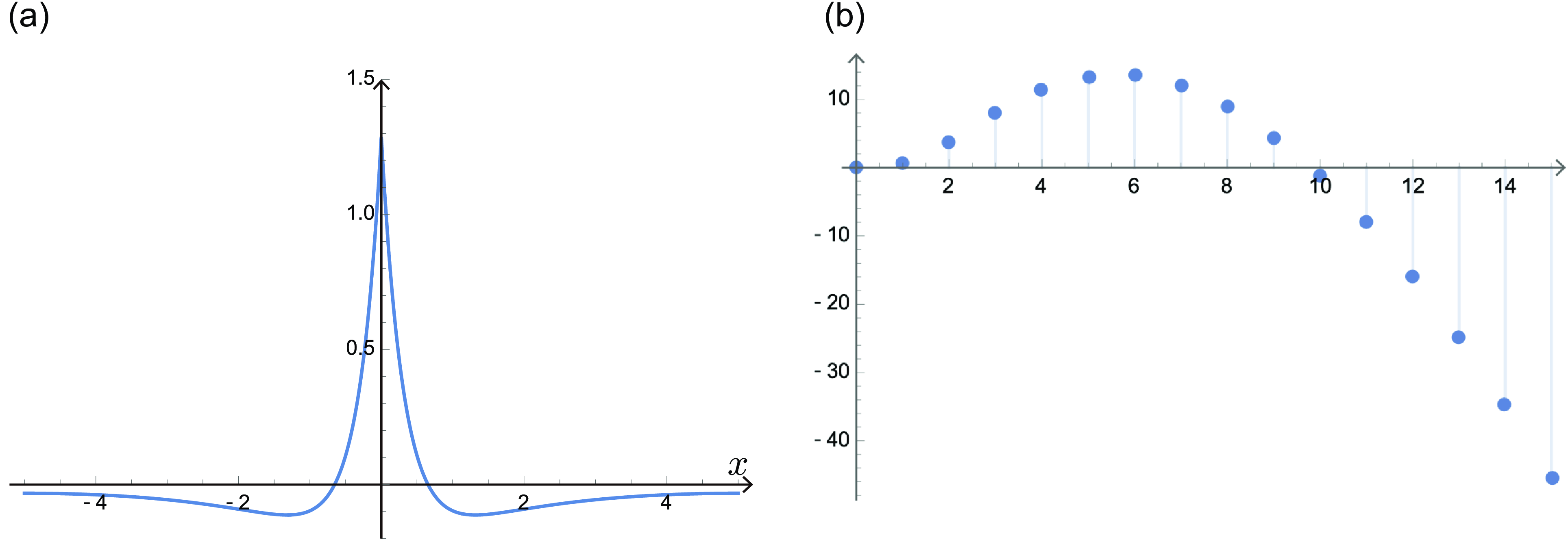
 ωn,1
ωn,1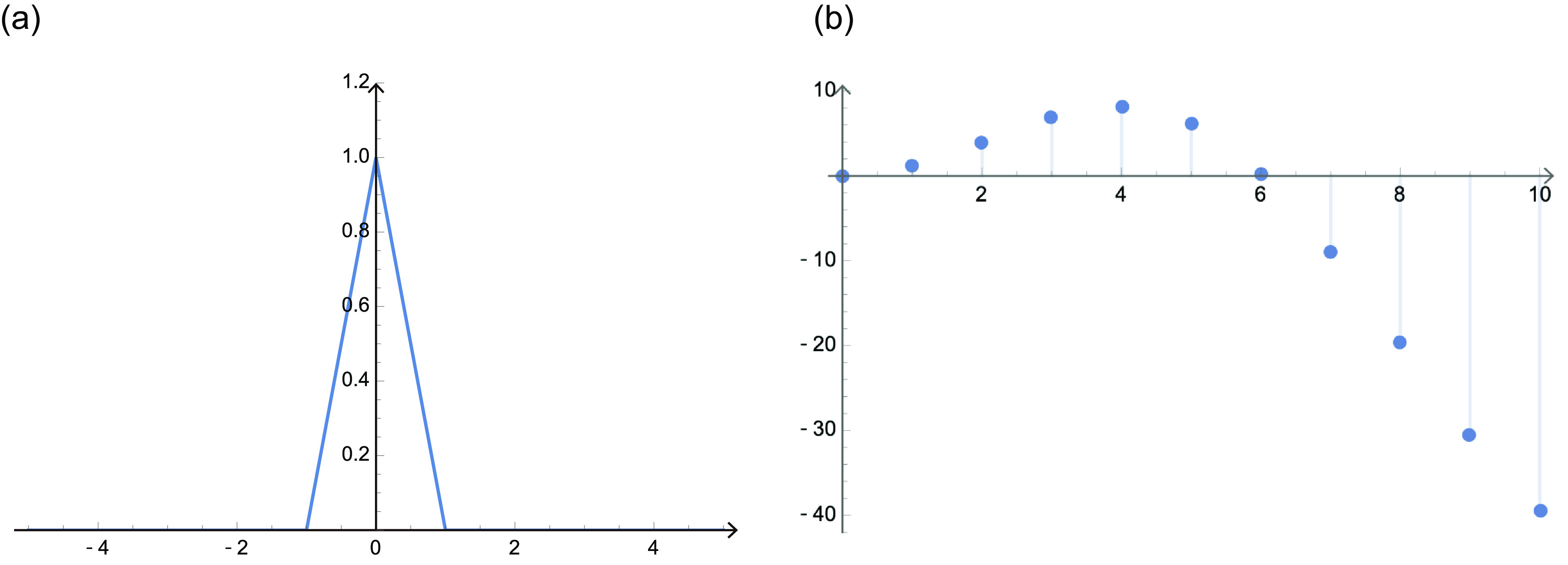
 ωn,2
ωn,2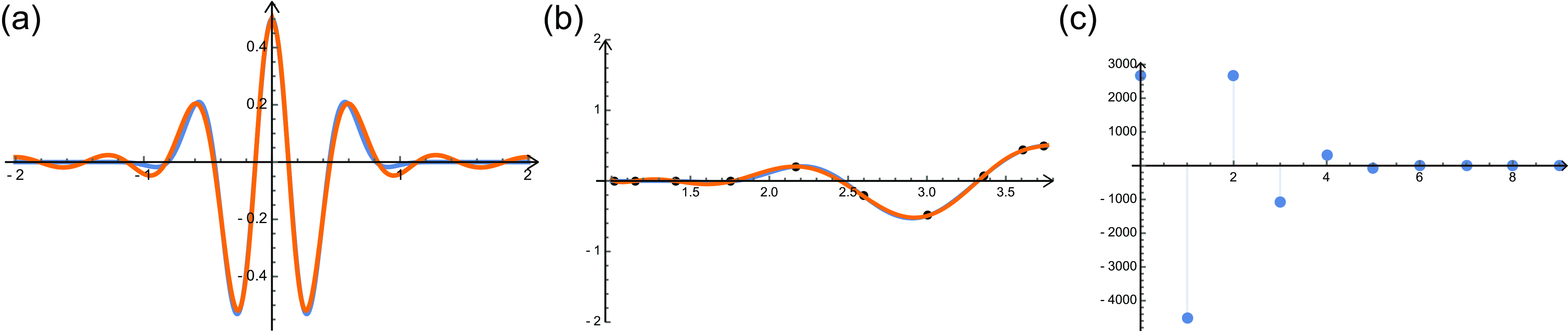
 W
W coshj(L−|x|)
 W(x)=e−5x2(cos(3π)x−1/2cos(2πx))
 L=2
L=2 W
W coshj(L−|x|)
 f
f [1,coshL]
 {αj9}j=09
 W(x)=e−5x2
 μ
μ Pμ
Pμ KSM,ε
KSM,ε M=7
M=7 L=1
L=1 ε=0.001
 d1=1000000
 μ=5
μ=5 dj
dj aj
aj t=200.0
 x
x ρ
ρ ρ
ρ KSM,ε
KSM,ε t=200.0
 ρ7,ε
ρ7,ε ρ
ρ (vj)0=kj∗ρ0, (j=1,…,M)
 (ρ7,ε,{vj7,ε}j=17)
 W
W ∑j=06αj6cosh(j(L−|x|))
 W
W ∑j=06αj6cosh(j(L−|x|))
 {αj6}j=06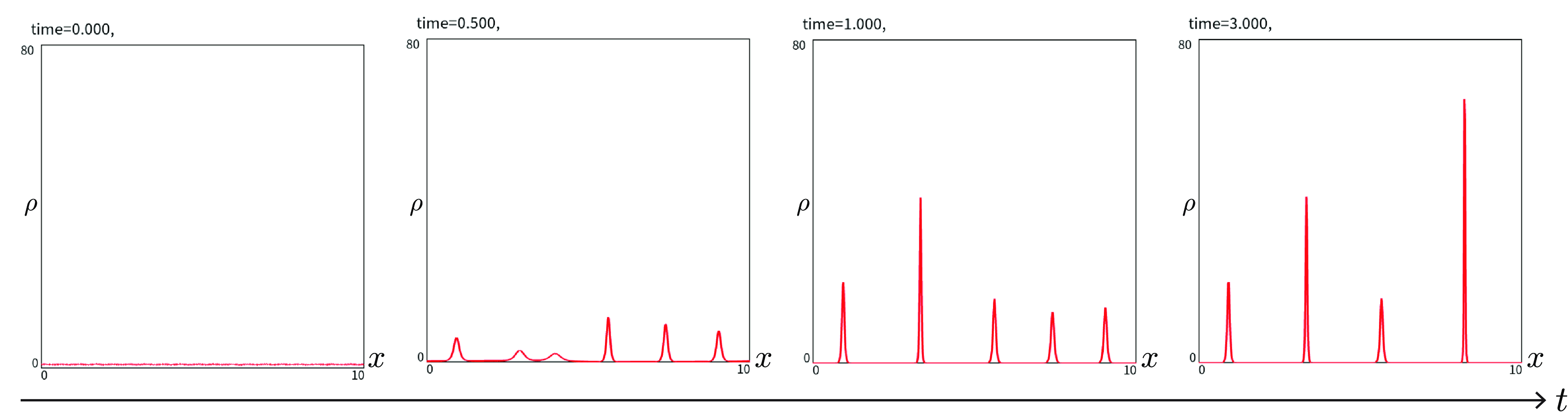
 Pμ
Pμ μ=5.0
μ=5.0 d1=0.1
 d2=3.0
 1.0
1.0 x
x ρ
ρ ρ
ρ Pμ
Pμ [0,10]
 t=0,0.5,1.0
 3.0
3.0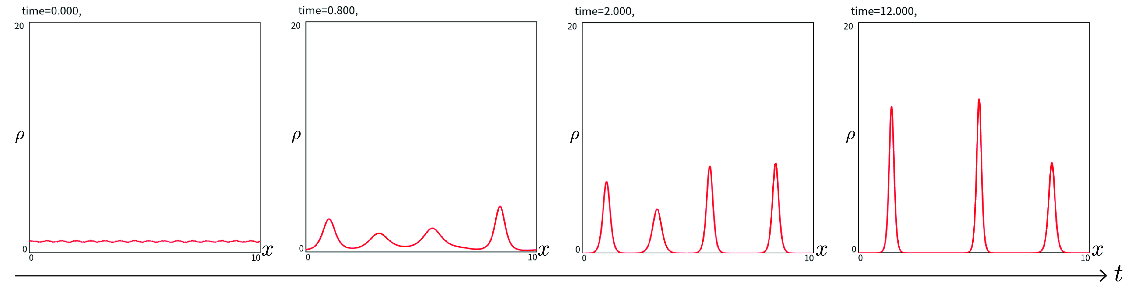
 Pμ
Pμ μ=4.0
μ=4.0 R=1.0
R=1.0 1.0
1.0 x
x ρ
ρ ρ
ρ Pμ
Pμ [0,10]
 t=0,0.8,2.0
 12.0
12.0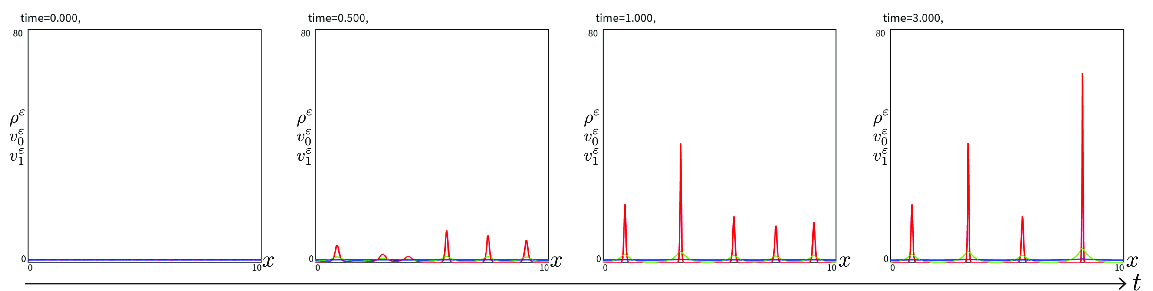
 μ,d1,d2
 ε=0.001
 ((v1)0,(v2)0)=(k1∗ρ0,k2∗ρ0)
 x
x ρε
ρε v1ε
v1ε v2ε
v2ε ρε
ρε v1ε
v1ε v2ε
v2ε [0,10]
 t=0,0.5,1.0
 3.0
3.0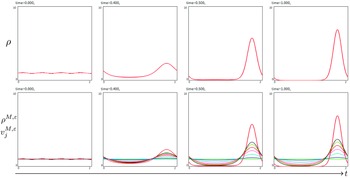
 t=1.0
t=1.0
 Open access

