


1. Introduction
Multirotor unmanned aerial vehicles (UAVs) generate lift using three or more rotors. They have become a successful, cost-effective means for diverse applications such as surveillance, visual inspection, precision agriculture, and mapping. UAVs equipped with manipulators have also demonstrated effectiveness in contact inspection tasks for infrastructure maintenance [Reference Zeng, Zhong, Wang, Fan and Zhang1]. According to a 2020 survey involving over 220 companies,Footnote 1 the primary motivations for adopting UAVs are saving costs and time and improving quality and workplace safety. However, the performance of UAVs varies significantly depending on the mission. Each mission has a specific desired performance objective that ideally must be considered in UAV design. Traditionally, UAVs are designed based on empirical methods that rely on experimental data and experience-based selection procedures to obtain the most satisfactory flight performance, which are uneconomical and inefficient. The number of actuators also plays a significant role in the design. One set of hardware for a quadcopter can deliver the optimal design, while for a hexacopter, the same hardware may not necessarily give the desired response. Competing parameters are another challenge in designing UAVs. For example, increasing the propeller’s diameter provides more thrust for a given rotor speed, but the increased inertia makes the system less responsive. Also, aerodynamic performance and structural parameters sometimes have a complex coupling relationship. That is why a systematic approach to designing UAVs is essential. It enhances the UAV performance and makes it possible to quickly assess changes’ effects on the desired mission. Optimization-based techniques can supply the best solution based on the mission requirements.
During design optimization, the aim is to find the optimal combination of design features that will give the best performance in some sense. Lim et al. [Reference Lim, Kim, Yee and Yee2] presented a mission-oriented performance assessment algorithm for UAVs as an overall design optimization procedure. They developed practical estimation models for frame weight and drag estimations and propulsion system analysis. The frame weight and frame aerodynamic models were based on the geometric configuration of the UAV. The propulsion system analysis model estimated the variation in the motor efficiency depending on the components of the multirotor and the flight conditions. In another study, a generic and efficient sizing methodology was presented to optimize the configuration design of the UAV based on the desired mission (endurance, maximum take-off acceleration, and maximum climb rate) using multidisciplinary design optimization techniques [Reference Delbecq, Budinger, Ochotorena, Reysset and Defay3]. A formulation for the best endurance condition regarding battery capacity and hover time was proposed. Using the blade element theory, an analytical expression was derived to design new configurations to satisfy given requirements regarding flight time, take-off weight, and prototyping costs [Reference Angelis, Angelis, Giulietti, Rossetti, Ianiro and Bellani4]. An optimized propulsion system, by using a genetic intelligent optimization algorithm, was designed and validated for the forward state of a quadcopter. The optimal results showed that the shape of rotors appropriate for hovering and forward flight is significantly different [Reference Angelis, Angelis, Giulietti, Rossetti, Ianiro and Bellani4]. A surrogate-model-based multi-objective optimization method was proposed for the preliminary design of the UAV. The objective function was based on the UAV’s storage capacity in the entire fuselage area and thrust-to-weight ratio [Reference Zhu, Li, Nie, Wei and Wei6].
The maneuverability of the UAV is another factor that has been considered in many optimizations. By using actuator time constants and the inertia of the craft to measure the performance, Magnussen et al. [Reference Magnussen, Hovland and Ottestad7] optimized the UAV maneuverability performance. Another study estimated the optimal propulsion system parameters according to maneuverability requirements. They used the ratio of hover thrust to the maximum thrust as a measure of maneuverability [Reference Dai, Quan, Ren and Cai8]. With a similar ratio, Dai et al. proposed a practical method to automatically calculate the optimal UAV design according to the flight time, altitude, payload capacity, and maneuverability [Reference Dai, Quan and Cai9]. They also proposed a practical method to help designers quickly determine the optimal propulsion system to maximize the UAV efficiency under the desired flight condition [Reference Dai, Quan, Ren and Cai10].
The ability of the UAV to hold a position in a wind field is vital for various commercial applications. This capability is particularly critical for emerging industrial use cases such as autonomous delivery drones, where position stability directly impacts package placement accuracy and safety during the final approach to drop zones. Similarly, in precision agriculture, stable hovering enables accurate sensor readings and precise application of treatments, while search and rescue operations in windy conditions require UAVs that can maintain stable positions while scanning areas or delivering emergency supplies. These industrial applications increasingly demand UAVs that can operate reliably in varied environmental conditions, making wind disturbance rejection a key performance differentiator. This can be achieved through using robust controllers or modifying the physical design. Nevertheless, testing control algorithms on actual UAVs can pose significant challenges, including safety risks and possible damage to equipment. To bridge this gap between simulation and real-world implementation, hardware-in-the-loop simulation approaches have proven valuable. Xian et al. developed a testbed that provides an intermediate step between pure simulation and full flight testing, which is particularly relevant when evaluating a UAV’s response to disturbances like wind [Reference Xian, Zhao, Zhang and Zhang11]. In this study, however, we are not focused on the control design. One method whereby rejection of these stochastic components can be eased is by passively tilting the rotors. There are studies focused on manipulating the tilt angles, or rotor positions, for maximizing agility [Reference Mehmood, Nakamura and Johnson12, Reference Hashem, Kuipers, Engelen and Stramigioli13]. Whidborne and Cooke demonstrated the rotor tilt’s effect on a quadcopter gust rejection response [Reference Whidborne and Cooke14]. They demonstrated that designing the vehicle with an outwards rotor tilt potentially results in a dramatic improvement in the gust rejection properties of the UAV.
In another study, a multi-objective optimization problem was proposed in which the objective function components were the robustness and the energy indexes. They optimized the tilt of a UAV in a heterogeneous manner [Reference Arellano-Quintana, Portilla-Flores and Merchán-Cruz15]. Fully-actuated UAVs can produce forces and torques in any direction, including the horizontal plane (vectored thrust), as opposed to conventional UAVs, which must tilt to translate. Tilting is limited by the rotational inertia of the aircraft, which limits the bandwidth of the actuation. Meanwhile, fully-actuated UAVs and their ability to directly generate lateral forces have significantly higher actuation bandwidths (i.e. frequency range over which the UAV’s actuators can effectively respond to control inputs) (increased responsiveness), making disturbance rejection easier. There have been attempts to optimize control plants for UAV disturbance rejection and closed-loop control qualities like bandwidth [Reference Zhang, Sun, Liu, Liu and Ye16, Reference Morari17, Reference Wang, Wang, Li and Mao18]. Beyond standard optimization approaches, advanced control techniques have been developed to enhance UAV stability in challenging conditions [Reference Khadhraoui, Zouaoui and Saad19]. Also, cooperative control strategies for UAVs have shown promising results in enhancing system robustness. Thebe et al. [Reference Thebe, Jamisola and Ramalepa20] demonstrated a novel approach using relative Jacobian formulations to holistically control multiple drones as paired units. Månsson and Stenberg worked on the development of a mechanical design of UAVs and a control algorithm to maximize the wind resistance [Reference Månsson and Stenberg21]. They employed the balancing power usage and position error to assess underactuated UAVs. Nevertheless, this study only compared two different time constants in the controller and used one propeller type while ignoring the bandwidth effects. Chen et al. included bandwidth as the primary objective function of fully-actuated UAVs to ensure that wind disturbance rejection controllers are not limited [Reference Chen, Stol and Richards22]. They integrated models for rotor performance, UAV component masses, and expected disturbances from turbulence to find the fastest response and most compact UAV for a particular payload and hover time. Recent experimental work by Bannwarth et al. [Reference Bannwarth, Kazemi and Stol23] has demonstrated the effectiveness of frequency-dependent H∞ control for wind disturbance rejection on a fully-actuated tilted-rotor octocopter, with wind tunnel tests validating performance at various wind speeds.
The main contribution of this study is to develop a simple correlation function (by using a consistent controller generation procedure) that can be used as an analog for the achievable control performance of fully-actuated UAVs under wind disturbance. Unlike previous works that rely on exhaustive dynamic simulations, this work introduces a simplified metric for UAV design optimization, enabling rapid assessment of disturbance rejection performance. This approach facilitates UAV parameter selection without requiring full-state nonlinear modeling, making it a practical tool for early-stage UAV design. It extracts simple design characteristics from octocopter models developed prior and then explores their relationship with the closed-loop disturbance rejection. To find these relationships, we compare the performance across multiple different octocopter configurations, each varying in their UAV radius, rotor tilt angle, payload capacity, and rotor-propeller specifications. All configurations are evaluated under consistent conditions. This systematic comparison enables us to analyze how physical parameter variations affect disturbance rejection performance and identify key relationships between design characteristics and control effectiveness.
This paper is organized as follows. Section 2 describes the nonlinear model of the tilted octocopter. The model undergoes simplification in the full-state linear model and the simplified model (reduced-state linear model). Then, the characteristics are extracted from the simplified model. Section 3 concentrates on the optimal tuning of the controller since control performance ought to be considered in the model for performance assessment. This is vital to achieve fair comparisons amongst multiple UAVs. Section 4 establishes relationships between the extracted simplified model parameters and the disturbance rejection performance in the same simplified model. Ultimately, the predictions of the simplified model are extended to the nonlinear model in Section 5, with subsection Section 5.4 providing experimental validation of the underlying principles through wind tunnel testing data that corroborates the effectiveness of our correlation function in predicting real-world UAV performance.
2. Dynamic modeling
This section provides an abridged summary of the components of the UAV model and how it is adapted for new dimensions or different components. A single-plane fully-actuator octocopter and its schematic are shown in Figures 1(a) and (b). The UAV analyzed in this study is a single-plane octocopter, chosen over a coaxial configuration after consideration of design trade-offs relevant to disturbance rejection performance. While Haddadi et al. [Reference Haddadi, Zarafshan and Dehghani24, Reference Haddadi and Zarafshan25] demonstrated that coaxial octocopter designs offer benefits in terms of increased thrust and payload capacity, our focus on dynamic wind disturbance rejection led us to prioritize different design characteristics. Although coaxial configurations offer compactness [Reference Haddadi and Zarafshan26], they introduce aerodynamic interference between vertically stacked rotors. This interference creates complex flow patterns that can reduce aerodynamic efficiency compared to planar configurations under identical motor specifications. For disturbance rejection applications specifically, this reduced efficiency directly impacts the achievable control bandwidth, which our study identifies as a critical factor for high-precision station-keeping. The planar configuration selected for this study maximizes the aerodynamic efficiency of each rotor and provides superior control authority for countering lateral wind forces without reorientation. Also, in contrast to underactuated UAVs that must tilt to generate lateral forces, a fully-actuated planar octocopter can immediately apply counteracting thrust in the horizontal plane, eliminating response delays and increasing the effective control bandwidth available for disturbance rejection.
(a) The schematic and (b) the actual photo of the fully actuated octocopter. (c) Demonstration of angles in a spherical representation of a vector.

Each rotor is rotated about either the body x or y axes to achieve full actuation. The parameters defining the octocopter are the UAV radius (
 ${r}_{{UAV}}$
), rotor tilt angle, payload, and rotor-propellor specifications. The modeling used in this work is derived from ref. [Reference Bannwarth, Kazemi and Stol23], where
${r}_{{UAV}}$
), rotor tilt angle, payload, and rotor-propellor specifications. The modeling used in this work is derived from ref. [Reference Bannwarth, Kazemi and Stol23], where
 ${r}_{{UAV}}=0.25\textrm{m}$
, and the propeller size is
${r}_{{UAV}}=0.25\textrm{m}$
, and the propeller size is
 $6^{\prime\prime}$
. The model components are depicted in Figure 2, where the output is
$6^{\prime\prime}$
. The model components are depicted in Figure 2, where the output is
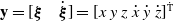 $\mathbf{y}=[\boldsymbol{\xi } \quad \dot{\boldsymbol{\xi }} ]=[ {x} \ {y} \ {z}\ {\dot{{x}}} \ {\dot{{y}}} \ \dot{{z}}]^{\dot{\mathrm{T}}}$
. The position is included to keep the UAV at a fixed point in space. Velocity is also kept as an output to supply feedback to the cascaded velocity loop in the control structure. The input and wind disturbance vectors are
$\mathbf{y}=[\boldsymbol{\xi } \quad \dot{\boldsymbol{\xi }} ]=[ {x} \ {y} \ {z}\ {\dot{{x}}} \ {\dot{{y}}} \ \dot{{z}}]^{\dot{\mathrm{T}}}$
. The position is included to keep the UAV at a fixed point in space. Velocity is also kept as an output to supply feedback to the cascaded velocity loop in the control structure. The input and wind disturbance vectors are
 $\mathbf{u}= [{F}_{{V}{,}{x}}\ {F}_{{V}{,}{y}}\ {F}_{{z}}]^{\mathrm{T}}\text{and }\mathbf{w}= [{u}\ {v}\ {w}]^{\mathrm{T}}$
, respectively, where the subscript V denotes vectored thrust commands that can be generated directly in the horizontal plane without changing the UAV’s orientation. Note that since in this work only the station keeping performance via vectored thrust is investigated, there are no torque commands (attitude-based accelerations) in u.
$\mathbf{u}= [{F}_{{V}{,}{x}}\ {F}_{{V}{,}{y}}\ {F}_{{z}}]^{\mathrm{T}}\text{and }\mathbf{w}= [{u}\ {v}\ {w}]^{\mathrm{T}}$
, respectively, where the subscript V denotes vectored thrust commands that can be generated directly in the horizontal plane without changing the UAV’s orientation. Note that since in this work only the station keeping performance via vectored thrust is investigated, there are no torque commands (attitude-based accelerations) in u.
Block diagram of the nonlinear UAV model showing attitude controllers, dynamics, aerodynamic models, and motor components. Inputs include thrust commands and wind disturbances, while outputs contain position and velocity states.

The internal states for the model are
 $\mathbf{x}= [\boldsymbol{\xi }\dot{\boldsymbol{\xi }}\ \mathbf{q}^{\mathbf{T}}\ ^{\boldsymbol{\mathcal{B}}}\boldsymbol{\nu }^{\mathbf{T}}\ \boldsymbol{\omega }^{\mathbf{T}}\ \mathbf{x}_{\mathbf{PID}}^{\mathbf{T}}]^{\mathrm{T}}$
, where
$\mathbf{x}= [\boldsymbol{\xi }\dot{\boldsymbol{\xi }}\ \mathbf{q}^{\mathbf{T}}\ ^{\boldsymbol{\mathcal{B}}}\boldsymbol{\nu }^{\mathbf{T}}\ \boldsymbol{\omega }^{\mathbf{T}}\ \mathbf{x}_{\mathbf{PID}}^{\mathbf{T}}]^{\mathrm{T}}$
, where
 $\mathbf{q}$
is the quaternion representing the orientation of the UAV (which is zero attitudes as we are in vectored thrust mode),
$\mathbf{q}$
is the quaternion representing the orientation of the UAV (which is zero attitudes as we are in vectored thrust mode),
 $\ ^{\mathcal{B}}\boldsymbol{\nu }$
is the vector of angular rates, and
$\ ^{\mathcal{B}}\boldsymbol{\nu }$
is the vector of angular rates, and
 $\boldsymbol{\omega }$
is the vector of rotor speeds. The state
$\boldsymbol{\omega }$
is the vector of rotor speeds. The state
 $\mathbf{x}_{\mathrm{PID}}$
(six states for roll and pitch PID and one state for yaw integratorFootnote
2
) represents the internal states of the attitude controller. The attitude controller has a cascade form, with an angular position controller, which outputs desired attitude rates
$\mathbf{x}_{\mathrm{PID}}$
(six states for roll and pitch PID and one state for yaw integratorFootnote
2
) represents the internal states of the attitude controller. The attitude controller has a cascade form, with an angular position controller, which outputs desired attitude rates
 $\boldsymbol{\nu }_{\mathrm{des}}$
. These are then passed into three angular rate controllers (one for each axis). The roll and pitch controllers are Proportional–Integral–Derivative (PID), with a second-order filter for each derivative component (three states each). In this work, we consider the attitude controller as a part of the plant. The rigid body dynamics are governed by Eq. (1),
$\boldsymbol{\nu }_{\mathrm{des}}$
. These are then passed into three angular rate controllers (one for each axis). The roll and pitch controllers are Proportional–Integral–Derivative (PID), with a second-order filter for each derivative component (three states each). In this work, we consider the attitude controller as a part of the plant. The rigid body dynamics are governed by Eq. (1),
 \begin{eqnarray}\ddot{\boldsymbol{\xi }}& =& g + \frac{1}{m_{t}} {}^{W}_{R} \textbf{R}\big({}^{B}\textbf{T} + ^{B}\textbf{F}_{\textrm{Aero}}\big)\\[3pt]\nonumber\dot{\textbf{v}} &=& \textbf{I}^{-1} \big({}^{B}\boldsymbol{\tau} - {}^{B}\textbf{v} \times (I{}^{B} v) + {}^{B}\boldsymbol{\tau}_{\textrm{Aero}}\big) \end{eqnarray}
where
 $\mathbf{g}$
represents the gravity acceleration,
$\mathbf{g}$
represents the gravity acceleration,
 $\mathrm{m}_{\mathrm{t}}$
the mass of the UAV,
$\mathrm{m}_{\mathrm{t}}$
the mass of the UAV,
 $\mathbf{I}$
the inertia tensor, and
$\mathbf{I}$
the inertia tensor, and
 ${\ }^{\mathcal{B}}{\boldsymbol{\nu }}{}$
the angular rate vector.
${\ }^{\mathcal{B}}{\boldsymbol{\nu }}{}$
the angular rate vector.
 ${\ }^{\mathcal{B}}{\mathbf{T}}{}$
and
${\ }^{\mathcal{B}}{\mathbf{T}}{}$
and
 ${\ }^{\mathcal{B}}{\boldsymbol{\tau }}{}$
are total forces and torques generated by all the motors, which are functions of the propellor geometry, wind characteristics, inflow angles (see Figure 1c), and angular speed of motors (represented by a nonlinear differential equation).
${\ }^{\mathcal{B}}{\boldsymbol{\tau }}{}$
are total forces and torques generated by all the motors, which are functions of the propellor geometry, wind characteristics, inflow angles (see Figure 1c), and angular speed of motors (represented by a nonlinear differential equation).
 ${\ }^{\mathcal{B}}{\mathbf{F}_{\text{Aero}}}{}\text{ and }{\ }^{\mathcal{B}}{\boldsymbol{\tau }_{\text{Aero}}}{}$
are frame aerodynamic forces and moments, depending on the wind angle and geometry of the UAV. These correlations are based upon the wind described in a spherical coordinate frame, with two angles
${\ }^{\mathcal{B}}{\mathbf{F}_{\text{Aero}}}{}\text{ and }{\ }^{\mathcal{B}}{\boldsymbol{\tau }_{\text{Aero}}}{}$
are frame aerodynamic forces and moments, depending on the wind angle and geometry of the UAV. These correlations are based upon the wind described in a spherical coordinate frame, with two angles
 ${\alpha}$
and
${\alpha}$
and
 ${\beta }$
(see Figure 1c) [Reference Bannwarth, Kazemi and Stol23]. Each new UAV is described by its dimensions and motor specifications. In most cases, the specific design parameters (such as rotor dimensions, motor specifications, material properties, and UAV geometry) can be directly substituted for each new UAV. Some quantities, however, need to be recalculated. For each UAV, the frame inertia is not available; as a result, the inertia is calculated using the same formula as ref. [Reference Chen, Stol and Richards22]. This treats motors as point masses at the ends of arms, arms as thin rods, and the battery and central frame as thin discs. While the input voltage was available from experiments in ref. [Reference Bannwarth, Kazemi and Stol23], in this work, it is estimated. For each motor, a linear relationship is assumed between the rotor speed and the PWM on a scale of 0 to 1, where
${\beta }$
(see Figure 1c) [Reference Bannwarth, Kazemi and Stol23]. Each new UAV is described by its dimensions and motor specifications. In most cases, the specific design parameters (such as rotor dimensions, motor specifications, material properties, and UAV geometry) can be directly substituted for each new UAV. Some quantities, however, need to be recalculated. For each UAV, the frame inertia is not available; as a result, the inertia is calculated using the same formula as ref. [Reference Chen, Stol and Richards22]. This treats motors as point masses at the ends of arms, arms as thin rods, and the battery and central frame as thin discs. While the input voltage was available from experiments in ref. [Reference Bannwarth, Kazemi and Stol23], in this work, it is estimated. For each motor, a linear relationship is assumed between the rotor speed and the PWM on a scale of 0 to 1, where
 ${\omega }{=}{c}_{{1}}{\chi }_{{1}}{+}{c}_{{2}}$
[Reference Chen, Stol and Richards22]Footnote
3
. Given an input PWM, this is used to generate an equivalent speed
${\omega }{=}{c}_{{1}}{\chi }_{{1}}{+}{c}_{{2}}$
[Reference Chen, Stol and Richards22]Footnote
3
. Given an input PWM, this is used to generate an equivalent speed
 ${\omega }_{{eq}}$
. Subsequently, by using the steady-state form of the motor speed model from ref. [Reference Bannwarth, Kazemi and Stol23], the resulting closed-form expression for the input voltage is achieved:
${\omega }_{{eq}}$
. Subsequently, by using the steady-state form of the motor speed model from ref. [Reference Bannwarth, Kazemi and Stol23], the resulting closed-form expression for the input voltage is achieved:
 \begin{equation} {V}_{\mathrm{i}}=\frac{{R}{c}_{{\tau }}}{{K}_{{T}}}{{\omega }_{{eq}}}^{2}+{K}_{{E}}{\omega }_{{eq}}+{I}_{{0}}{R}, \end{equation}
where
 ${R}$
is the internal resistance,
${R}$
is the internal resistance,
 ${I}_{{0}}$
is the idle current,
${I}_{{0}}$
is the idle current,
 ${V}_{{i}}$
the input current, and
${V}_{{i}}$
the input current, and
 ${c}_{{\tau }}$
the motor torque constant.
${c}_{{\tau }}$
the motor torque constant.
 ${K}_{{T}}={K}_{{E}}$
are the torque and back-emf constants respectively, while
${K}_{{T}}={K}_{{E}}$
are the torque and back-emf constants respectively, while
 ${K}_{{E}}$
can be computed from
${K}_{{E}}$
can be computed from
 ${K}_{{E}}{=}\frac{{V}_{{0}}{-}{I}_{{0}}{R}}{{K}_{{v}}{V}_{{0}}}$
where
${K}_{{E}}{=}\frac{{V}_{{0}}{-}{I}_{{0}}{R}}{{K}_{{v}}{V}_{{0}}}$
where
 ${V}_{{0}}$
is the motor’s nominal voltage and
${V}_{{0}}$
is the motor’s nominal voltage and
 ${K}_{{v}}$
is the motor speed constant [Reference Chen, Stol and Richards22]. Furthermore, the gains of the internal attitude controller are not immediately usable for different UAV sizes due to scaling effects. This is because when the length dimension l of a given UAV is changed, the moment of inertia will scale with l
2, whilst the moment produced for a given torque command will scale with l. This nonlinear relationship means that attitude controller gains optimized for one UAV size must be adjusted for larger or smaller craft. Because of this, attitude gains from ref. [Reference Bannwarth, Kazemi and Stol23], for the planar octocopter of radius 0.25 m, do not provide satisfactory control on larger UAVs. As such, a preliminary trim analysis and linearization are first undertaken to identify linear rotational dynamics.
${K}_{{v}}$
is the motor speed constant [Reference Chen, Stol and Richards22]. Furthermore, the gains of the internal attitude controller are not immediately usable for different UAV sizes due to scaling effects. This is because when the length dimension l of a given UAV is changed, the moment of inertia will scale with l
2, whilst the moment produced for a given torque command will scale with l. This nonlinear relationship means that attitude controller gains optimized for one UAV size must be adjusted for larger or smaller craft. Because of this, attitude gains from ref. [Reference Bannwarth, Kazemi and Stol23], for the planar octocopter of radius 0.25 m, do not provide satisfactory control on larger UAVs. As such, a preliminary trim analysis and linearization are first undertaken to identify linear rotational dynamics.
To identify the linear rotation dynamics, a transfer function from pitch torque
 ${T}{(}{s}{)}$
to angular acceleration
${T}{(}{s}{)}$
to angular acceleration
 ${s}^{{2}}{\unicode{x1D6E9}}({s})$
is created. The gain of this transfer function implies the scaling in the rotational dynamics. A scaling value is then added to the plant’s torque commands to compensate for this scaling discrepancy, such that the attitude gains from ref. [Reference Bannwarth, Kazemi and Stol23] are still usable. For linearization, the hover throttle corresponding to a 5.6 m/s wind condition is used as the operating point, though the linearization itself is performed with a still-air model. This is compared with a reference linearization of the original octocopter [Reference Chen, Stol and Richards22], performed under still-air conditions. This comparison yields a scaling factor for torque commands that compensates for size-related differences in rotational dynamics. The specific hover throttle selection has minimal impact on the final scaling factors for stability.
${s}^{{2}}{\unicode{x1D6E9}}({s})$
is created. The gain of this transfer function implies the scaling in the rotational dynamics. A scaling value is then added to the plant’s torque commands to compensate for this scaling discrepancy, such that the attitude gains from ref. [Reference Bannwarth, Kazemi and Stol23] are still usable. For linearization, the hover throttle corresponding to a 5.6 m/s wind condition is used as the operating point, though the linearization itself is performed with a still-air model. This is compared with a reference linearization of the original octocopter [Reference Chen, Stol and Richards22], performed under still-air conditions. This comparison yields a scaling factor for torque commands that compensates for size-related differences in rotational dynamics. The specific hover throttle selection has minimal impact on the final scaling factors for stability.
2.1. Simplified model
The complexity of the nonlinear model makes it difficult to find simple predictor parameters. As a preliminary simplifying step, the nonlinear model is first converted to a full-state linear model. After substituting the UAV parameters and rotational scaling values, the following process is undertaken. A trim point for each UAV is first specified. The wind vector is set to
 ${u}^{\mathrm{*}}=5.6\ \mathrm{m}/\mathrm{s}, {v}^{{*}}=\ {w}^{\mathrm{*}}=0\ \mathrm{m}/\mathrm{s}$
. By manipulating u, with wind constraint, trim analysis is conducted to find a valid operating point. After this, a MATLAB linearization tool is used to generate the final full-state linear model as
${u}^{\mathrm{*}}=5.6\ \mathrm{m}/\mathrm{s}, {v}^{{*}}=\ {w}^{\mathrm{*}}=0\ \mathrm{m}/\mathrm{s}$
. By manipulating u, with wind constraint, trim analysis is conducted to find a valid operating point. After this, a MATLAB linearization tool is used to generate the final full-state linear model as
 \begin{eqnarray}\dot{\mathbf{x}}&=&\mathbf{Ax}+\ \mathbf{B}_{\mathrm{u}}\mathbf{u}+\ \mathbf{B}_{\mathrm{d}}\mathbf{w}\nonumber\\[4pt]\mathbf{y}&=&\mathbf{Cx}+\mathbf{D}_{\mathrm{u}}\mathbf{u}+\mathbf{D}_{\mathrm{d}}\mathbf{w}\end{eqnarray}
where,
 $\mathbf{A}\in {\mathbb{R}^{28\times 28}},\mathbf{B}_{\mathrm{u}}\in \mathbb{R}^{28\times 3},\mathbf{B}_{\mathrm{d}}\in \mathbb{R}^{28\times 3},\mathbf{C}\in \mathbb{R}^{6\times 28},\mathbf{D}_{\mathrm{u}}\in \mathbb{R}^{6\times 3},\ \mathbf{D}_{\mathrm{d}}\in \mathbb{R}^{6\times 3}$
. After truncation, this linearization process leads to the transfer function matrix
$\mathbf{A}\in {\mathbb{R}^{28\times 28}},\mathbf{B}_{\mathrm{u}}\in \mathbb{R}^{28\times 3},\mathbf{B}_{\mathrm{d}}\in \mathbb{R}^{28\times 3},\mathbf{C}\in \mathbb{R}^{6\times 28},\mathbf{D}_{\mathrm{u}}\in \mathbb{R}^{6\times 3},\ \mathbf{D}_{\mathrm{d}}\in \mathbb{R}^{6\times 3}$
. After truncation, this linearization process leads to the transfer function matrix
 ${G}_{{full}}({s})$
. With this linearization complete, we can now develop our simplified model,
${G}_{{full}}({s})$
. With this linearization complete, we can now develop our simplified model,
 $G_{simp}(s)$
. This simplified model aims to capture the core features of the dynamics while allowing the investigation of performance through a small set of parameters. The simplified model describes the UAV as a single-degree-of-freedom mass system, including a band-limited actuator. This simplicity in modeling is afforded by the use of vectored thrust for position regulation, allowing the omission of attitude dynamics. Outside of the mass, the primary dynamics are those of the band-limited actuator. This is modeled as a low-pass filter, which accounts for the limits in how fast motor speeds can be changed (see Figure 3). These parameters are in part influenced by the heuristics discussed in ref. [Reference Morari17], where the impact of the control input on the controlled output should be maximized (so called actuator gain
$G_{simp}(s)$
. This simplified model aims to capture the core features of the dynamics while allowing the investigation of performance through a small set of parameters. The simplified model describes the UAV as a single-degree-of-freedom mass system, including a band-limited actuator. This simplicity in modeling is afforded by the use of vectored thrust for position regulation, allowing the omission of attitude dynamics. Outside of the mass, the primary dynamics are those of the band-limited actuator. This is modeled as a low-pass filter, which accounts for the limits in how fast motor speeds can be changed (see Figure 3). These parameters are in part influenced by the heuristics discussed in ref. [Reference Morari17], where the impact of the control input on the controlled output should be maximized (so called actuator gain
 ${K}_{\mathrm{act}}$
), and the time constant on the actuator should be minimized (
${K}_{\mathrm{act}}$
), and the time constant on the actuator should be minimized (
 $1/{\omega }_{{c}}$
). The inclusion of the actuator bandwidth (
$1/{\omega }_{{c}}$
). The inclusion of the actuator bandwidth (
 $\omega_{c}$
) reflects the works like ref. [Reference Chen, Stol and Richards22], which prioritize bandwidth for disturbance rejection, whilst
$\omega_{c}$
) reflects the works like ref. [Reference Chen, Stol and Richards22], which prioritize bandwidth for disturbance rejection, whilst
 $K_{act}$
reflects prioritization of the force production ability [Reference Hashem, Kuipers, Engelen and Stramigioli13].
$K_{act}$
reflects prioritization of the force production ability [Reference Hashem, Kuipers, Engelen and Stramigioli13].
Simplified model block diagram capturing key parameters for disturbance rejection analysis:
 $\mathrm{K}_{\mathrm{act}}$
is the actuator gain and
$\mathrm{K}_{\mathrm{act}}$
is the actuator gain and
 $\mathrm{K}_{aero}$
is the aerodynamic gain.
$\mathrm{K}_{aero}$
is the aerodynamic gain.
 ${\unicode[Arial]{x03C9}} _{\mathrm{c}}$
is the actuator bandwidth. C(s) is the position controller block, X(s) is the output, U(s) and F(s) are inputs.
${\unicode[Arial]{x03C9}} _{\mathrm{c}}$
is the actuator bandwidth. C(s) is the position controller block, X(s) is the output, U(s) and F(s) are inputs.

To generate a simplified model for a given UAV, the linearization is first truncated to inputs, disturbances, and position output for the x-axis. To match the simplified and the full-state linear model, their acceleration transfer functions must match, where
 $s^{2}\ G_{full} (s) \cong s^{2} G_{simp} (s)$
.
$s^{2}\ G_{full} (s) \cong s^{2} G_{simp} (s)$
.
 \begin{equation}\left[\begin{array}{cc} {s}^{2}{G}_{{full}{,}11}{(}{s}{)} & {s}^{2}{G}_{{full}{,}12}{(}{s}{)} \end{array}\right]\cong \left[\begin{array}{cc} \dfrac{{K}_{{aero}}}{{m}} & \dfrac{{K}_{{act}}}{{m}{(}\frac{{s}}{{\omega }_{{c}}}{+}1{)}} \end{array}\right]\end{equation}
where,
 ${G}_{{full}{,}11}{(}{s}{)}$
represents the transfer function from input
${G}_{{full}{,}11}{(}{s}{)}$
represents the transfer function from input
 ${U}{(}{s}{)}$
to position
${U}{(}{s}{)}$
to position
 ${X}{(}{s}{)}$
, and
${X}{(}{s}{)}$
, and
 ${G}_{{full}{,}12}({s})$
represents the transfer function from
${G}_{{full}{,}12}({s})$
represents the transfer function from
 ${F}{(}{s}{)}$
to position X
${F}{(}{s}{)}$
to position X
 ${(}{s}{)}$
. Note that
${(}{s}{)}$
. Note that
 ${G}_{{full}}({s})$
is the linearization of the nonlinear model and its block diagram is the same as Figure 2. Using Eq. (4),
${G}_{{full}}({s})$
is the linearization of the nonlinear model and its block diagram is the same as Figure 2. Using Eq. (4),
 ${K}_{{aero}}{/}{m}$
can be found by equating it to the mean passband gain of
${K}_{{aero}}{/}{m}$
can be found by equating it to the mean passband gain of
 ${s}^{2}{G}_{{full}{,}11}{(}{s}{)}$
. The value of m was taken from the UAV parameters, facilitating the evaluation of
${s}^{2}{G}_{{full}{,}11}{(}{s}{)}$
. The value of m was taken from the UAV parameters, facilitating the evaluation of
 ${K}_{{aero}}$
. Meanwhile,
${K}_{{aero}}$
. Meanwhile,
 ${K}_{{act}}$
was found from the passband gain of
${K}_{{act}}$
was found from the passband gain of
 ${s}^{{2}}{G}_{{full}{,}{12}}{(}{s}{)}$
. Finally,
${s}^{{2}}{G}_{{full}{,}{12}}{(}{s}{)}$
. Finally,
 ${\omega }_{{c}}$
is found by equating it to the upper cut-off frequency of
${\omega }_{{c}}$
is found by equating it to the upper cut-off frequency of
 ${s}^{{2}}{G}_{{full}{,}{21}}{(}{s}{)}$
. This acceleration-based matching approach is chosen because it captures the essential force-mass dynamics that dominate position control performance, while allowing higher-order effects to be simplified. By matching transfer functions at the acceleration level rather than position, the reduced model preserves the critical dynamic relationships between inputs and resultant accelerations that determine disturbance rejection capability.
${s}^{{2}}{G}_{{full}{,}{21}}{(}{s}{)}$
. This acceleration-based matching approach is chosen because it captures the essential force-mass dynamics that dominate position control performance, while allowing higher-order effects to be simplified. By matching transfer functions at the acceleration level rather than position, the reduced model preserves the critical dynamic relationships between inputs and resultant accelerations that determine disturbance rejection capability.
 ${G}_{{simp}}{(}{s}{)}$
provides substantial computational benefits while maintaining sufficient predictive accuracy for comparative analysis.
${G}_{{simp}}{(}{s}{)}$
provides substantial computational benefits while maintaining sufficient predictive accuracy for comparative analysis.
 ${G}_{{full}}({s})$
requires evaluation of 28 state variables at 248 Hz, demanding significant computational resources for each UAV configuration. In contrast, the reduced-state model with only three key parameters (
${G}_{{full}}({s})$
requires evaluation of 28 state variables at 248 Hz, demanding significant computational resources for each UAV configuration. In contrast, the reduced-state model with only three key parameters (
 ${K}_{{aero}}$
,
${K}_{{aero}}$
,
 ${K}_{{act}}$
, and
${K}_{{act}}$
, and
 ${\omega }_{{c}}$
), enables rapid evaluation, reducing simulation time by approximately 95 %. This efficiency allowed us to comprehensively analyze 500 different UAV configurations, an analysis scope that would be prohibitively time-consuming with the full model. When validated against full nonlinear simulations in Section 5, the simplified model demonstrates strong correlation with actual performance rankings, confirming that it preserves the essential dynamic relationships necessary for comparative design analysis. While absolute performance predictions may differ from full nonlinear results, the relative rankings of UAV configurations remain consistent, making this approach particularly valuable for early-stage design optimization where rapid comparative assessment is more critical than absolute performance prediction.
${\omega }_{{c}}$
), enables rapid evaluation, reducing simulation time by approximately 95 %. This efficiency allowed us to comprehensively analyze 500 different UAV configurations, an analysis scope that would be prohibitively time-consuming with the full model. When validated against full nonlinear simulations in Section 5, the simplified model demonstrates strong correlation with actual performance rankings, confirming that it preserves the essential dynamic relationships necessary for comparative design analysis. While absolute performance predictions may differ from full nonlinear results, the relative rankings of UAV configurations remain consistent, making this approach particularly valuable for early-stage design optimization where rapid comparative assessment is more critical than absolute performance prediction.
This simplified modeling approach deliberately focuses on the core physical parameters most relevant to disturbance rejection performance. The model reduction extracts only the three most influential parameters while maintaining the essential dynamic relationships that determine disturbance rejection capability. The simplified model does not aim to predict absolute performance values, but rather to establish relative performance rankings that remain consistent when evaluated using the full nonlinear model, making it an effective tool for early-stage UAV design optimization.
The linearization process involves several assumptions that support the modeling approach. Linearization occurs around an operating point (wind speed u* = 5.6 m/s) that represents typical operational conditions for station-keeping tasks. The aerodynamic coefficients scaling from the validated octocopter model to different geometries follow established dimensional analysis principles, with the simplified model capturing the essential dynamics as demonstrated in Figure 3. While the linearization naturally simplifies some coupling effects between axes and assumes quasi-steady wind conditions, these simplifications are appropriate for the primary disturbance rejection analysis presented. The strong correlation between the simplified metrics and full nonlinear simulation performance validates that these modeling decisions effectively capture the fundamental relationships between UAV design parameters and disturbance rejection capability. It’s worth noting that while this simplified model is tailored for fully-actuated UAVs, a similar approach could potentially be adapted for underactuated systems, though this would require incorporating attitude dynamics to account for the inherent coupling between lateral motion and orientation in such platforms.
Note that when using frame aerodynamic forces and moments for new UAVs (in Section 2), the characteristic dimensions, including the distance between opposite motor centers and the planar disc formed by the UAV’s body and motors, are varied while keeping the model coefficients the same. Table I summarizes the relationships between the UAV’s characteristic dimensions and the corresponding model parameters, illustrating how each physical attribute influences the aerodynamic and actuation behavior of the system.
The linearization at a single wind speed represents a deliberate modeling decision that balances simplicity with practical relevance. While real-world conditions include time-varying wind profiles, the quasi-steady assumption allows us to establish consistent comparative metrics across different UAV configurations. Although our approach omits attitude dynamics for fully-actuated UAVs, this simplification is justified since vectored thrust permits position control without orientation changes. This decoupling enables the reduced-order model to focus exclusively on the parameters dominating disturbance rejection performance. The model’s predictive limitations are acknowledged and partially addressed through validation against full nonlinear simulations in Section 5, which demonstrates that despite these simplifications, the relative performance rankings of different configurations remain consistent.
Influence of characteristic dimensions on UAV model parameters and their scaling relationships.

3. Optimal control tuning
Disturbance rejection performance is sensitive to the choice of position controller, C(s), and its gains. This section discusses how the position controller tuning is carried out automatically to ensure fair comparisons. The assessment of UAVs is posed as an optimal control problem, which minimizes the position variation under the wind disturbance while maintaining constant actuator usage. This can be formulated as the
 ${H}_{2}$
norms of the system. The
${H}_{2}$
norms of the system. The
 ${H}_{2}$
norm of a generic transfer function is given by
${H}_{2}$
norm of a generic transfer function is given by
 $\left\| {G} (s) \right\| _{2}=\sqrt{\frac{1}{2{\unicode[Arial]{x03C0}} }\int _{-\infty}^{\infty} G\left(j\omega\right)G^{*}\left(j\omega\right){d}{\omega }}$
, which represents the root mean square error of the output, under a unit variance signal at the input. Note that this is equivalent to the energy usage when responding to a unit impulse input (Parseval’s theorem). According to Figure 3, the plant
$\left\| {G} (s) \right\| _{2}=\sqrt{\frac{1}{2{\unicode[Arial]{x03C0}} }\int _{-\infty}^{\infty} G\left(j\omega\right)G^{*}\left(j\omega\right){d}{\omega }}$
, which represents the root mean square error of the output, under a unit variance signal at the input. Note that this is equivalent to the energy usage when responding to a unit impulse input (Parseval’s theorem). According to Figure 3, the plant
 ${G}_{simp}(s)$
(including
${G}_{simp}(s)$
(including
 $K_{aero}$
,
$K_{aero}$
,
 $ {K}_{act}/\frac{s}{\omega_{c}} + 1$
, and
$ {K}_{act}/\frac{s}{\omega_{c}} + 1$
, and
 $1/ms^{2}$
) has two inputs of the wind speed
$1/ms^{2}$
) has two inputs of the wind speed
 $U(s)$
and control command
$U(s)$
and control command
 $F(s)$
.
$F(s)$
.
The dynamics can be manipulated through the free parameters in the controller
 ${C}{(}{s}{)}.$
Two transfer functions of
${C}{(}{s}{)}.$
Two transfer functions of
 ${D}{(}{s}{)}\,{=}\,{X}{(}{s}{)}{/}{U}{(}{s}{)}$
and
${D}{(}{s}{)}\,{=}\,{X}{(}{s}{)}{/}{U}{(}{s}{)}$
and
 ${V}{(}{s}{)}\,{=}\,{F}{(}{s}{)}{/}{U}{(}{s}{)}$
are of interest.
${V}{(}{s}{)}\,{=}\,{F}{(}{s}{)}{/}{U}{(}{s}{)}$
are of interest.
 ${D}{(}{s}{)}$
represents the position accuracy of the UAV to the wind, where lower magnitudes imply smaller variation under the disturbance. Meanwhile
${D}{(}{s}{)}$
represents the position accuracy of the UAV to the wind, where lower magnitudes imply smaller variation under the disturbance. Meanwhile
 ${V}{(}{s}{)}$
represents the efficiency of the UAV. If
${V}{(}{s}{)}$
represents the efficiency of the UAV. If
 ${V}{(}{s}{)}$
is small for a given wind, the UAV’s actuator usage will be small. In finding the optimal position performance for a given UAV, minimizing
${V}{(}{s}{)}$
is small for a given wind, the UAV’s actuator usage will be small. In finding the optimal position performance for a given UAV, minimizing
 $\| {D}{(}{s}{)}\| _{{2}}$
while keeping
$\| {D}{(}{s}{)}\| _{{2}}$
while keeping
 $\| {V}{(}{s}{)}\| _{{2}}$
below some limit is of interest (minimizing the impact of a disturbance, whilst maintaining consistent energy usage). Note that the value of
$\| {V}{(}{s}{)}\| _{{2}}$
below some limit is of interest (minimizing the impact of a disturbance, whilst maintaining consistent energy usage). Note that the value of
 $\| {D}{(}{s}{)}\| _{{2}}$
with the optimal gains will be denoted
$\| {D}{(}{s}{)}\| _{{2}}$
with the optimal gains will be denoted
 $\| {D}({s})\| _{{2}}^{{*}}$
.
$\| {D}({s})\| _{{2}}^{{*}}$
.
For all UAVs, the input to the plant passes through the same multirotor mixer [Reference Bannwarth, Kazemi and Stol23]. This multirotor mixer generates throttles for the eight rotors (between 0 and 100). Therefore, constraining V
 ${(}{s}{)}$
is analogous to constraining the motor usage, as a fraction of the full range of the motor. This, however, does not account for how close the operating point is to rotor saturation. Hence, the constraint on
${(}{s}{)}$
is analogous to constraining the motor usage, as a fraction of the full range of the motor. This, however, does not account for how close the operating point is to rotor saturation. Hence, the constraint on
 $\| {V}{(}{s}{)}\| _{{2}}$
is scaled based on the amount of throttle headroom available at hover. This is described in Eq. (5), where
$\| {V}{(}{s}{)}\| _{{2}}$
is scaled based on the amount of throttle headroom available at hover. This is described in Eq. (5), where
 ${\chi }_{{ hover}}$
denotes the hover throttle (on a [0 1] scale) and
${\chi }_{{ hover}}$
denotes the hover throttle (on a [0 1] scale) and
 ${M}_{{ base}}$
is a scaling factor applied. The subscript d in
${M}_{{ base}}$
is a scaling factor applied. The subscript d in
 ${\chi }_{{d}}$
denotes the idea of distance from the minimum/maximum limits of the actuators.
${\chi }_{{d}}$
denotes the idea of distance from the minimum/maximum limits of the actuators.
 \begin{eqnarray}\chi_{d} &=& min(\chi_{hover}, 1-\chi_{hover})\nonumber\\&&\parallel V (s)\parallel_{2}\, \leq\, \chi_{d}\ M_{base} .\end{eqnarray}
Note that, whilst imperfect, the used hover throttles are those for still air operation. It means the actuator constraint is in terms of the percentage of the maximum possible force being used. For each UAV,
 ${\chi }_{{ hover}}$
is determined from the hover throttle and motor properties. Systune (MATLAB control systems toolbox) is used to study the control performance of linear models by specifying the control problem with
${\chi }_{{ hover}}$
is determined from the hover throttle and motor properties. Systune (MATLAB control systems toolbox) is used to study the control performance of linear models by specifying the control problem with
 $\mathrm{H}_{2}$
norms. In the control optimization, the plant is also modified with a low-pass filter (
$\mathrm{H}_{2}$
norms. In the control optimization, the plant is also modified with a low-pass filter (
 ${\omega }_{{cut}}=5\,\textrm{rad}/\textrm{s}$
and passband gain of 0.32) added to the input
${\omega }_{{cut}}=5\,\textrm{rad}/\textrm{s}$
and passband gain of 0.32) added to the input
 $\mathrm{U}(\mathrm{s})$
to reflect the turbulence characteristics of the wind to be used later in simulation. Systune is used to optimize the gains for controllers with the PID form. Based on the actuator usage for the original octocopter when rejecting wind,
$\mathrm{U}(\mathrm{s})$
to reflect the turbulence characteristics of the wind to be used later in simulation. Systune is used to optimize the gains for controllers with the PID form. Based on the actuator usage for the original octocopter when rejecting wind,
 ${M}_{{ base}}=0.015$
. The value reflects the typical throttle headroom available at hover for the specific motors and control system in use in [Reference Månsson and Stenberg21]. While the scaling factor is not derived from a theoretical framework, it provides a practical constraint to ensure motor utilization remains within an efficient operating range, preventing excessive throttle demands that might lead to saturation or inefficient control.
${M}_{{ base}}=0.015$
. The value reflects the typical throttle headroom available at hover for the specific motors and control system in use in [Reference Månsson and Stenberg21]. While the scaling factor is not derived from a theoretical framework, it provides a practical constraint to ensure motor utilization remains within an efficient operating range, preventing excessive throttle demands that might lead to saturation or inefficient control.
4. Disturbance rejection performance trends
The first fit is taken by sourcing feasible UAVs under constraints for optimization [Reference Chen, Stol and Richards22]. 500 UAVs are chosen such that
 $m_{pay} = 1\textrm{kg}\, ;\, T_{flight} \geq 5\, \textrm{minutes} \,;\, T H_{max} \geq 3.5\textrm{N}$
. Then, the linearization and control described in Sections 2 and 3 are applied to these 500 chosen UAVs. Curve fitting is used to establish relationships between simplified model parameters and the disturbance rejection performance. A logarithmic transformation is applied to the data as depicted in Eq. (6).
$m_{pay} = 1\textrm{kg}\, ;\, T_{flight} \geq 5\, \textrm{minutes} \,;\, T H_{max} \geq 3.5\textrm{N}$
. Then, the linearization and control described in Sections 2 and 3 are applied to these 500 chosen UAVs. Curve fitting is used to establish relationships between simplified model parameters and the disturbance rejection performance. A logarithmic transformation is applied to the data as depicted in Eq. (6).
 \begin{equation} \log \left(\left\| {D}\left({s}\right)\right\| _{{2}}^{{*}}\right)\sim \log \left({m}\right)+\log \left({\omega }_{{c}}\right)+\log \left({K}_{{act}}{\chi }_{{d}}\right)+\log ({K}_{{aero}}). \end{equation}
 $\| {D}({s})\| _{{2}}^{{*}}$
is generated by optimization on the simplified model. In Eq. (6),
$\| {D}({s})\| _{{2}}^{{*}}$
is generated by optimization on the simplified model. In Eq. (6),
 ${K}_{{act}}{\chi }_{{d}}$
is the scaled actuator gain and m is the mass of the whole UAV. The value for
${K}_{{act}}{\chi }_{{d}}$
is the scaled actuator gain and m is the mass of the whole UAV. The value for
 ${\chi }_{{d}}$
could be calculated directly from the hover throttle as
${\chi }_{{d}}$
could be calculated directly from the hover throttle as
 $\ {\chi }_{{d}}=\min ({\alpha}{,}{1}{-}{\alpha}),\text{ where}\, {\alpha}=\frac{{{\omega }_{{hover}}}{-}{c}_{{2}}}{{c}_{{1}}}100$
. As applying the linearization processes in Sections 2 and 3 was expensive, based on the original fits, we estimated the simplified model parameters for 10,000 crafts (from their raw specifications). For example, actuator gain taken as
$\ {\chi }_{{d}}=\min ({\alpha}{,}{1}{-}{\alpha}),\text{ where}\, {\alpha}=\frac{{{\omega }_{{hover}}}{-}{c}_{{2}}}{{c}_{{1}}}100$
. As applying the linearization processes in Sections 2 and 3 was expensive, based on the original fits, we estimated the simplified model parameters for 10,000 crafts (from their raw specifications). For example, actuator gain taken as
 ${K}_{{act}}=\frac{3.6TH_{\max}}{\chi_{d}}+2.1$
, and aerodynamic gain was calculated as
${K}_{{act}}=\frac{3.6TH_{\max}}{\chi_{d}}+2.1$
, and aerodynamic gain was calculated as
 ${K}_{{aero}}=14.4{R}_{{UAV}}^{{2}}-4.4{R}_{{UAV}}+0.84$
.
${K}_{{aero}}=14.4{R}_{{UAV}}^{{2}}-4.4{R}_{{UAV}}+0.84$
.
These UAVs were chosen from optimization results [Reference Chen, Stol and Richards22] for every possible pairwise combination of the time of flight
 ${T}_{{flight}}=(1.5,5,10,15,50)\text{ min}$
and the payload
${T}_{{flight}}=(1.5,5,10,15,50)\text{ min}$
and the payload
 ${m}_{{pay}}=(0.3,3,10,30)\text{ kg}$
. The maximum horizontal thrust,
${m}_{{pay}}=(0.3,3,10,30)\text{ kg}$
. The maximum horizontal thrust,
 ${T}{H}_{max }$
, is kept constant at 3.5 N. The reason is that
${T}{H}_{max }$
, is kept constant at 3.5 N. The reason is that
 ${T}_{{flight}}$
and
${T}_{{flight}}$
and
 ${m}_{{pay}}$
are equality constraints and changing them guarantees that new UAVs are generated; this was the only way to generate high-mass UAVs. Meanwhile, force requirements are inequality constraints. This means that if the force requirement for a given optimization is increased, the increased feasible UAVs are a subset of the original ones. The
${m}_{{pay}}$
are equality constraints and changing them guarantees that new UAVs are generated; this was the only way to generate high-mass UAVs. Meanwhile, force requirements are inequality constraints. This means that if the force requirement for a given optimization is increased, the increased feasible UAVs are a subset of the original ones. The
 ${T}{H}_{max }$
is also kept constant, as lower force requirements can lead to less wind rejection capability (even with
${T}{H}_{max }$
is also kept constant, as lower force requirements can lead to less wind rejection capability (even with
 ${T}{H}_{max }\geq 3.5\mathrm{N}$
, still some UAVs are not survivable at a 5.6 m/s wind).
${T}{H}_{max }\geq 3.5\mathrm{N}$
, still some UAVs are not survivable at a 5.6 m/s wind).
The response of the performance against the two dominant variables of
 ${K}_{{aero}}$
and
${K}_{{aero}}$
and
 ${K}_{{act}}{\chi }_{{d}}$
, for the 10,000 crafts, is shown in Figure 4. In this fit, there is a curvature, whereby the gradients are steeper for more precise UAVs (better disturbance rejection performance). A criterion given in Eq. (7) is used to define data points in two separate regions.
${K}_{{act}}{\chi }_{{d}}$
, for the 10,000 crafts, is shown in Figure 4. In this fit, there is a curvature, whereby the gradients are steeper for more precise UAVs (better disturbance rejection performance). A criterion given in Eq. (7) is used to define data points in two separate regions.
Coefficients describing response of disturbance rejection performance to simplified model parameters. In the upper region, actuator and aerodynamic gains dominate, followed by mass. In the lower region, bandwidth becomes significantly more important (−2.56), indicating its crucial role in high-performance configurations.

Response of performance to simplified model parameters when a larger parameter set is used. The 3D scatter plot shows the relationship between disturbance rejection performance on the vertical axis and the two key parameters on the horizontal axes. The data points (in orange) demonstrate how lower aerodynamic susceptibility and higher actuator authority correlate with improved disturbance rejection capability (lower values on the vertical axis). The curvature in the data distribution indicates that the relationship between these parameters and performance is nonlinear.

 \begin{equation} a\log \left({K}_{{act}}{\chi }_{{d}}\right) \leq {c}+{b}\log ({K}_{{aero}}). \end{equation}
The coefficients in Eq. (7) can be manually adjusted to achieve appropriate fits. By tuning based on a case-by-case approach to approximately separate the two regions, the coefficients obtained are
 $a=1,{b}=1.3,{c}=1.2$
. The selection of these boundary coefficients was based on iterative analysis of prediction error distributions across various boundary definitions. Through iterative analysis, we selected these boundary coefficients (a, b, c) to effectively separate UAVs with different control behavior patterns, resulting in improved fit quality within each region as evidenced by the distinct coefficient sets in Table II. This separation aligns with the physical principles of control systems, where aircraft with higher actuation-to-aerodynamic ratios can achieve distinct control bandwidths. The area, including points that typically have lower actuator gain than aerodynamics gain, is called the upper region, which has poorer performance. For practical implementation of this correlation function in UAV design, see Appendix A.
$a=1,{b}=1.3,{c}=1.2$
. The selection of these boundary coefficients was based on iterative analysis of prediction error distributions across various boundary definitions. Through iterative analysis, we selected these boundary coefficients (a, b, c) to effectively separate UAVs with different control behavior patterns, resulting in improved fit quality within each region as evidenced by the distinct coefficient sets in Table II. This separation aligns with the physical principles of control systems, where aircraft with higher actuation-to-aerodynamic ratios can achieve distinct control bandwidths. The area, including points that typically have lower actuator gain than aerodynamics gain, is called the upper region, which has poorer performance. For practical implementation of this correlation function in UAV design, see Appendix A.
The corresponding coefficients when fits are applied are shown in Table II. In this table,
 ${\beta }_{{m}}$
represents the mass influence, where a negative coefficient indicates that increasing mass improves disturbance rejection by increasing inertial resistance to wind forces.
${\beta }_{{m}}$
represents the mass influence, where a negative coefficient indicates that increasing mass improves disturbance rejection by increasing inertial resistance to wind forces.
 ${\beta }_{{{\omega }_{{c}}}}$
represents bandwidth, which affects the UAV’s ability to rapidly respond to disturbances. Note how
${\beta }_{{{\omega }_{{c}}}}$
represents bandwidth, which affects the UAV’s ability to rapidly respond to disturbances. Note how
 ${\beta }_{{{\omega }_{{c}}}}$
becomes significantly more important in the lower region (−2.56) compared to the upper region (−0.05).
${\beta }_{{{\omega }_{{c}}}}$
becomes significantly more important in the lower region (−2.56) compared to the upper region (−0.05).
 ${\beta }_{{{K}_{{act}}}{{.}{\chi }_{{d}}}}$
represents actuator gain scaled by hover throttle, with its larger magnitude in the lower region (−8.15 vs −3.19) showing that actuator capability becomes increasingly critical for precise control.
${\beta }_{{{K}_{{act}}}{{.}{\chi }_{{d}}}}$
represents actuator gain scaled by hover throttle, with its larger magnitude in the lower region (−8.15 vs −3.19) showing that actuator capability becomes increasingly critical for precise control.
 ${\beta }_{{{K}_{{aero}}}}$
represents aerodynamic susceptibility, where the positive coefficients indicate that larger aerodynamic forces degrade performance, with a stronger effect in the lower region (8.61 vs 4.14).
${\beta }_{{{K}_{{aero}}}}$
represents aerodynamic susceptibility, where the positive coefficients indicate that larger aerodynamic forces degrade performance, with a stronger effect in the lower region (8.61 vs 4.14).
Table II shows that the most critical variables are the actuator and aerodynamic gains. In the upper region (points that satisfy the constraints in Eq. (7)), the third most significant variable is the mass, while for the lower region, it is the bandwidth. For UAVs with low precision (high position norms under disturbance rejection), increasing mass will tend to decrease the variation in position under a wind disturbance. Ultimately, this mass increase is unlikely to be utilized. First and foremost, mass typically comes at the cost of efficiency [Reference Zhu, Li, Nie, Wei and Wei6]. Note that while these coefficients are derived from simulations with random sampling components, multiple executions of the analysis show that the coefficients remain highly stable, with only minor variations across different random samples of 10,000 UAVs.
While increasing the mass appears to improve performance, this is not usable, as the corresponding increase in the size of the UAV will make it excessively unfavorable aerodynamically. Since the aerodynamic coefficient has a more significant effect, it will likely overpower any benefits from increasing mass. Meanwhile, this also indicates that increasing bandwidth will improve disturbance rejection performance, but only for UAVs with a small position norm. At any level of precision, it is shown that an increase in the horizontal thrust authority or a decrease in aerodynamic gain will also improve disturbance rejection performance. The physical interpretation of the decrease in aerodynamic gain is a change in the characteristic area of the UAV (changes influence this through the radius and propellers). However, as shown in Table III for the UAVs in the lower region, there is significant coupling between
 ${K}_{{aero}}$
and
${K}_{{aero}}$
and
 ${K}_{{act}}\ {\cdot }{\chi }_{{d}}$
. This can be further overcome by varying the parameters independently.
${K}_{{act}}\ {\cdot }{\chi }_{{d}}$
. This can be further overcome by varying the parameters independently.
As the multicollinearity issues were not entirely solved in the prior fit, Figure 5a shows the variation in performance when the simplified model parameters are varied independently. For each simplified model parameter set (
 ${m}{,}\,{\omega }_{{c}}{,}\,{K}_{{act}}{,}\,{K}_{{aero}}$
), from the extended values generated from the optimizations discussed prior, the 1st and 99th percentiles are found and set as a bound as
${m}{,}\,{\omega }_{{c}}{,}\,{K}_{{act}}{,}\,{K}_{{aero}}$
), from the extended values generated from the optimizations discussed prior, the 1st and 99th percentiles are found and set as a bound as
 ${X}_{{low}}$
and
${X}_{{low}}$
and
 ${X}_{{high}}$
.
${X}_{{high}}$
.
Correlation coefficients amongst explanatory variables with first extended fit.

Response of optimal disturbance rejection performance when parameters are varied independently. (a) response to both aerodynamic and actuator gains. (b) demonstration of increase in residual errors when actuator and aerodynamic gains alone are used to explain performance.

Then new parameters are generated as
 ${x}_{{i}}=10^{\log \ {{X}_{{low}}}{+}{rlog}\frac{{X}_{{high}}}{{X}_{{low}}}}.$
This generates simplified model parameters, which are distributed logarithmically between a minimum and maximum value. This is repeated 10,000 times. Randomization is also applied across the
${x}_{{i}}=10^{\log \ {{X}_{{low}}}{+}{rlog}\frac{{X}_{{high}}}{{X}_{{low}}}}.$
This generates simplified model parameters, which are distributed logarithmically between a minimum and maximum value. This is repeated 10,000 times. Randomization is also applied across the
 ${\chi }_{{d}}$
values, whereby they are sampled from a uniform distribution on [0.2 0.5]. Ultimately, for the upper region, the resulting coefficients are the same. However, Figure 5b (reflecting a rotation of Figure 5a) makes clear that the explanatory power of
${\chi }_{{d}}$
values, whereby they are sampled from a uniform distribution on [0.2 0.5]. Ultimately, for the upper region, the resulting coefficients are the same. However, Figure 5b (reflecting a rotation of Figure 5a) makes clear that the explanatory power of
 ${K}_{{aero}}$
and
${K}_{{aero}}$
and
 ${K}_{{act}}\ {\cdot }{\chi }_{{d}}$
is highly attenuated in the precise region (with lower position norm). The fit coefficients for the lower region in this extended fit are
${K}_{{act}}\ {\cdot }{\chi }_{{d}}$
is highly attenuated in the precise region (with lower position norm). The fit coefficients for the lower region in this extended fit are
 ${\beta }_{{m}}=-1,{\beta }_{{{\omega }_{{c}}}}=-3.6,{\beta }_{{{K}_{{act}}}{{.}{\chi }_{{d}}}}=-2.6\text{ and }{\beta }_{{{K}_{{aero}}}}=3.5.$
Ultimately, this plot shows that bandwidth is equally essential when high precision is required (in the lower region, the variance in
${\beta }_{{m}}=-1,{\beta }_{{{\omega }_{{c}}}}=-3.6,{\beta }_{{{K}_{{act}}}{{.}{\chi }_{{d}}}}=-2.6\text{ and }{\beta }_{{{K}_{{aero}}}}=3.5.$
Ultimately, this plot shows that bandwidth is equally essential when high precision is required (in the lower region, the variance in
 $\| {D}{(}{s}{)}\| _{{2}}$
is much higher than in the upper region, and the bandwidth is not used in this plot while having a high coefficient compared to mass). However, these results fail to reflect the constraints on the feasibility of the UAV.
$\| {D}{(}{s}{)}\| _{{2}}$
is much higher than in the upper region, and the bandwidth is not used in this plot while having a high coefficient compared to mass). However, these results fail to reflect the constraints on the feasibility of the UAV.
5. Applying correlation functions to nonlinear models
The simulations were conducted using Simulink, incorporating the Control System Toolbox and Aerospace Blockset. The nonlinear UAV model operated with a 248 Hz control loop. Wind disturbances were modeled as a band-limited white noise process, with a mean wind speed of 5.6 m/s, replicating real-world turbulence effects. The Simulink model included various blocks such as an apparent wind speed model, aerodynamic model, motor model, UAV structural model, and comprehensive sensor models. The sensor modeling incorporates realistic noise and latency characteristics for each sensor type: IMU sensors following MPU-9250 specifications (0.012 m/s2 accelerometer noise, 0.1°/s gyroscope noise, 400 Hz sampling, 2.5 ms computational delays), motion capture system (1 mm RMS position noise, 100 ms processing delay), barometric altimeter (33 cm RMS altitude noise), and magnetometer with realistic sampling rate conversion. A Local Position Estimator performs multi-sensor fusion with covariance estimation and health monitoring. UAV parameters, including rotor thrust and aerodynamic coefficients, were derived from prior experimental studies. The actuation model accounted for motor lag and power constraints, ensuring practical feasibility. Controller gains were optimized using Systune, as mentioned in the previous section. A 15 dB stability margin was enforced across all simulations.
While our primary simulations use a mean wind speed of 5.6 m/s in the x-axis for consistency in comparing UAV designs, it should be noted that the wind model incorporates 10% turbulence intensity, adding significant dynamic variation to the flow conditions. This turbulence introduces fluctuations in both wind speed and direction, partially addressing multi-directional disturbance effects. The focus on a single primary wind direction allows us to isolate the fundamental relationships between design parameters and disturbance rejection performance without conflating directional effects.
The simplified model has facilitated the development of a characteristic for comparing the closed-loop disturbance rejection performance of fully-actuated UAVs. This section assesses this characteristic’s utility on more realistic models, i.e. the original nonlinear model discussed in Section 2 (including a sensor model and entire attitude controller). It also follows a similar optimization process to Section 3, with some modifications. Firstly, rather than PID, a P-PID cascade structure is used (see Figure 6), as it more accurately reflects the default control structure in the standard flight controller (PX4 firmware).Footnote
4
Systune could be used to formulate this; however, optimization could not be carried out with the P-PID gains as free variables, as it leads to poor control performance. Nonetheless, by analyzing the P-PID structure shown in Figure 6, for
 ${R}{(}{s}{)}=0$
we see that the dynamics between
${R}{(}{s}{)}=0$
we see that the dynamics between
 ${F}{(}{s}{)}$
and
${F}{(}{s}{)}$
and
 ${X}{(}{s}{)}$
are equivalent to that of a PID controller with a double derivative term (PIDD2).
${X}{(}{s}{)}$
are equivalent to that of a PID controller with a double derivative term (PIDD2).
 \begin{eqnarray} {F}({s})&=&\left({K}_{{pv}}+{K}_{{iv}}\ \frac{{1}}{{s}}\right)\left(-{K}_{{px}}{X}-{sX}\right)-{K}_{{dv}}{s\ }{\cdot }{sX}({s})\nonumber\\& =&\left(-{K}_{{pv}}{K}_{{px}}-{K}_{{iv}}-{K}_{{px}}{K}_{{iv}}\frac{{1}}{{s}}-{K}_{{pv}}{s}-{K}_{{dv}}{s}^{{2}}\right){X}({s}).\end{eqnarray}
Table IV summarizes all the controller notations. The term
 ${K}_{{pv}}{K}_{{px}}$
represents the direct use of position for position tracking, while
${K}_{{pv}}{K}_{{px}}$
represents the direct use of position for position tracking, while
 ${K}_{{iv}}$
involves the integration of a velocity component. Using the
${K}_{{iv}}$
involves the integration of a velocity component. Using the
 ${K}_{{iv}}$
alone to facilitate proportional components in the controller is undesirable, as it will lead to drift. This issue is solved in the conversion. By optimizing for the PIDD2 controller, the gain set
${K}_{{iv}}$
alone to facilitate proportional components in the controller is undesirable, as it will lead to drift. This issue is solved in the conversion. By optimizing for the PIDD2 controller, the gain set
 ${\unicode{x1D6EC}}_{{p}}{,}\,{\unicode{x1D6EC}}_{{i}}{,}\,{\unicode{x1D6EC}}_{{d}}{,}\,{\unicode{x1D6EC}}_{{{d}^{{2}}}}$
is obtained. By equating these gains to their respective terms in Eq. (8), the expressions
${\unicode{x1D6EC}}_{{p}}{,}\,{\unicode{x1D6EC}}_{{i}}{,}\,{\unicode{x1D6EC}}_{{d}}{,}\,{\unicode{x1D6EC}}_{{{d}^{{2}}}}$
is obtained. By equating these gains to their respective terms in Eq. (8), the expressions
 ${K}_{{dv}}{=}{\Lambda }_{{{d}^{\ 2}}}$
,
${K}_{{dv}}{=}{\Lambda }_{{{d}^{\ 2}}}$
,
 ${K}_{{pv}}{=}{\Lambda }_{{d}}$
,
${K}_{{pv}}{=}{\Lambda }_{{d}}$
,
 ${K}_{{px}}{=}\frac{{\Lambda }_{{p}}{\pm }\sqrt{{\Lambda }_{{p}}^{{2}}{-}{4}{\Lambda }_{{d}}{\Lambda }_{{i}}}}{{2}{\Lambda }_{{d}}}$
, and
${K}_{{px}}{=}\frac{{\Lambda }_{{p}}{\pm }\sqrt{{\Lambda }_{{p}}^{{2}}{-}{4}{\Lambda }_{{d}}{\Lambda }_{{i}}}}{{2}{\Lambda }_{{d}}}$
, and
 ${K}_{{iv}}{=}{\Lambda }_{{i}}{/}{K}_{{px}}$
hold.
${K}_{{iv}}{=}{\Lambda }_{{i}}{/}{K}_{{px}}$
hold.
Block diagram showing the layout of the P-PID cascaded structure.

Note that in Eq. (8), the larger of the two permitted
 ${K}_{{px}}$
is chosen to avoid the drift issue. Also, when
${K}_{{px}}$
is chosen to avoid the drift issue. Also, when
 ${K}_{{px}}$
is complex, the real part is taken. This generates acceptable results when the control performance is poor enough not to be affected by modeled sensor delay. However, for the cases when delay is significant, it can destabilize some UAVs. This is compensated for with an open-loop margin constraint of
${K}_{{px}}$
is complex, the real part is taken. This generates acceptable results when the control performance is poor enough not to be affected by modeled sensor delay. However, for the cases when delay is significant, it can destabilize some UAVs. This is compensated for with an open-loop margin constraint of
 ${G}_{{M}}=15\text{ dB},{\phi }_{{M}}=15^{\circ}$
. These values are chosen by trial and error. Nevertheless, this optimization method is unable to remove steady-state errors effectively. The stability margins (
${G}_{{M}}=15\text{ dB},{\phi }_{{M}}=15^{\circ}$
. These values are chosen by trial and error. Nevertheless, this optimization method is unable to remove steady-state errors effectively. The stability margins (
 ${G}_{{M}}=15\text{ dB},{\phi }_{{M}}=15^{\circ}$
) were selected based on established control system design guidelines for multirotor systems, falling within typical ranges used in flight control systems. This optimization method is unable to remove steady-state errors effectively. However, this limitation does not undermine our comparative analysis. Our research focuses on identifying superior UAV design characteristics for disturbance rejection rather than developing complete flight control systems. For station-keeping applications under persistent wind disturbances, dynamic rejection capability is more critical than precise steady-state tracking, as evidenced by our experimental results showing acceptable position errors and successful disturbance rejection performance across different UAV configurations. The bandwidth-dependent characteristics and transient response properties that determine disturbance rejection capability remain the primary metrics of interest in this comparative study.
${G}_{{M}}=15\text{ dB},{\phi }_{{M}}=15^{\circ}$
) were selected based on established control system design guidelines for multirotor systems, falling within typical ranges used in flight control systems. This optimization method is unable to remove steady-state errors effectively. However, this limitation does not undermine our comparative analysis. Our research focuses on identifying superior UAV design characteristics for disturbance rejection rather than developing complete flight control systems. For station-keeping applications under persistent wind disturbances, dynamic rejection capability is more critical than precise steady-state tracking, as evidenced by our experimental results showing acceptable position errors and successful disturbance rejection performance across different UAV configurations. The bandwidth-dependent characteristics and transient response properties that determine disturbance rejection capability remain the primary metrics of interest in this comparative study.
Summary of controller notations.

5.1. Simulation results with a nonlinear model
A 60-second simulation is run for each UAV, and the end of the simulation is used to assess the standard deviation (same wind trajectory for all tests). This optimization applies to the x-axis dynamic only, with a trim point based around
 ${u}^{{*}}=5.6\,\textrm{m}/\textrm{s}.$
Meanwhile, for the y-axis, the mean wind speed is
${u}^{{*}}=5.6\,\textrm{m}/\textrm{s}.$
Meanwhile, for the y-axis, the mean wind speed is
 $0\,\textrm{m}/\textrm{s}$
. As a result, the same controller will be non-optimal. Furthermore, the controller for the z-axis is not optimized at all, and the gains are constant throughout. For measuring the position, the standard deviation in position
$0\,\textrm{m}/\textrm{s}$
. As a result, the same controller will be non-optimal. Furthermore, the controller for the z-axis is not optimized at all, and the gains are constant throughout. For measuring the position, the standard deviation in position
 ${\sigma }_{{X}}$
is used to measure variation in the x-axis. The UAVs used here are the original 500 to which the methodology in Sections 2 and 3 was applied. Figure 7 shows the simulation results for the same simplified model variables from the prior section under the same wind trajectory. In the left sub-plot of Figure 7, the vertical axis is the log of the standard deviation in position. In the right sub-plot of Figure 7, the vertical axis is the standard deviation in the force command provided to the multirotor mixer, scaled by
${\sigma }_{{X}}$
is used to measure variation in the x-axis. The UAVs used here are the original 500 to which the methodology in Sections 2 and 3 was applied. Figure 7 shows the simulation results for the same simplified model variables from the prior section under the same wind trajectory. In the left sub-plot of Figure 7, the vertical axis is the log of the standard deviation in position. In the right sub-plot of Figure 7, the vertical axis is the standard deviation in the force command provided to the multirotor mixer, scaled by
 ${\chi }_{{d}}$
(the amount of PWM headroom). In the control optimization for the nonlinear model, a margin constraint is added to improve stability.
${\chi }_{{d}}$
(the amount of PWM headroom). In the control optimization for the nonlinear model, a margin constraint is added to improve stability.
In the final controller, one of the constraints will limit performance. It can then be observed from the right sub-plot of Figure 7 that most UAVs, which are limited by the actuation constraint in the optimization, maintain similar actuator levels (after scaling for
 ${\chi }_{{d}}$
) (orange dots). However, a limited number of outlier points are constrained by actuation according to optimization outputs (blue dots). These outlier points do not have the same actuation level as other UAVs. Throughout these simulation results, only the UAVs with
${\chi }_{{d}}$
) (orange dots). However, a limited number of outlier points are constrained by actuation according to optimization outputs (blue dots). These outlier points do not have the same actuation level as other UAVs. Throughout these simulation results, only the UAVs with
 ${\sigma }_{{X}}\lt 0.25\,\textrm{m}$
are presented. This filtering is added to ensure unstable UAVs are not incorporated into conclusions. At this stage, increasing the force authority and reducing the aerodynamic gain improve performance. This indicates that the simplified model’s characteristics are functional.
${\sigma }_{{X}}\lt 0.25\,\textrm{m}$
are presented. This filtering is added to ensure unstable UAVs are not incorporated into conclusions. At this stage, increasing the force authority and reducing the aerodynamic gain improve performance. This indicates that the simplified model’s characteristics are functional.
Variation in simulated optimal position control performance. (left) Position standard deviation response to simplified model variables. (right) Control action standard deviation response. Note that, as expected, most values in the actuation-limited set (which are constrained by available thrust authority), have very similar standard deviation in their control actions. This contrasts with the margin-limited UAVs (which are constrained by stability requirements), where the actuation usage begins to drop.

Distribution of simulation stability showing UAVs with active margin constraints (blue) versus actuation constraints (orange). Note that precise UAVs require margin constraints for stability. Total UAVs = 500.

This filtering approach effectively establishes an upper bound on the disturbance magnitude for which the control methodology remains effective. For the UAVs that passed this stability criterion (
 ${\sigma }_{{X}}\lt 0.25\,\textrm{m}$
), the control system demonstrated robust performance under the 5.6 m/s mean wind speed with 10% turbulence intensity. Beyond this level, some UAV configurations require either redesign of their physical parameters or more advanced control strategies to maintain acceptable performance. From Figure 7, including the margin constraint heavily distorts the curve. However, Figure 8 shows that precise UAVs (smaller position norms and better disturbance rejection performance) require the margin constraint to be stable in simulation. In fact, we need the margin constraint to keep the UAVs stable. To illustrate the practical performance of this approach, Figure 9 shows the time-domain response of a representative octocopter (selected as the median performer among 250 valid configurations with the median position error in the x-axis) during steady-state operation (t > 20 s to exclude transient effects). Position errors remain acceptable, with maximum x-axis deviation of approximately 0.25 m and smaller y and z variations (±0.05–0.1 m). Motor PWM commands range from 1150 to 1807
${\sigma }_{{X}}\lt 0.25\,\textrm{m}$
), the control system demonstrated robust performance under the 5.6 m/s mean wind speed with 10% turbulence intensity. Beyond this level, some UAV configurations require either redesign of their physical parameters or more advanced control strategies to maintain acceptable performance. From Figure 7, including the margin constraint heavily distorts the curve. However, Figure 8 shows that precise UAVs (smaller position norms and better disturbance rejection performance) require the margin constraint to be stable in simulation. In fact, we need the margin constraint to keep the UAVs stable. To illustrate the practical performance of this approach, Figure 9 shows the time-domain response of a representative octocopter (selected as the median performer among 250 valid configurations with the median position error in the x-axis) during steady-state operation (t > 20 s to exclude transient effects). Position errors remain acceptable, with maximum x-axis deviation of approximately 0.25 m and smaller y and z variations (±0.05–0.1 m). Motor PWM commands range from 1150 to 1807
 $\unicode{x03BC}$
s, well within the simulation model’s operating range of 1075–1950
$\unicode{x03BC}$
s, well within the simulation model’s operating range of 1075–1950
 $\unicode{x03BC}$
s, with clear differential actuation between motors demonstrating coordinated control adaptation to wind disturbances.
$\unicode{x03BC}$
s, with clear differential actuation between motors demonstrating coordinated control adaptation to wind disturbances.
Time-domain response of representative UAV showing position errors (top) and motor PWM commands (bottom) during wind disturbance rejection.

Figure 10 provides comprehensive verification of physical reasonability across 250 UAV configurations. The scatter plot shows PWM operating envelopes versus position error, where blue dots represent 90th percentile PWM values and red dots represent 10th percentile values. Percentiles are calculated individually for each of the eight motors, with the worst-case values (the highest 90th percentile and the lowest 10th percentile) across all motors selected to represent each UAV’s operating envelope, providing robust statistics unaffected by brief control spikes. The analysis reveals 90th percentile PWM values ranging from 1390 to 1950
 $\unicode{x03BC}$
s (mean: 1771
$\unicode{x03BC}$
s (mean: 1771
 $\unicode{x03BC}$
s) and 10th percentile values from 1127 to 1718
$\unicode{x03BC}$
s) and 10th percentile values from 1127 to 1718
 $\unicode{x03BC}$
s (mean: 1345
$\unicode{x03BC}$
s (mean: 1345
 $\unicode{x03BC}$
s), based on the motor model’s PWM constraints of 1075–1950
$\unicode{x03BC}$
s), based on the motor model’s PWM constraints of 1075–1950
 $\unicode{x03BC}$
s. Notably, 48.4% of configurations require high control effort (>1800
$\unicode{x03BC}$
s. Notably, 48.4% of configurations require high control effort (>1800
 $\unicode{x03BC}$
s) while 15.2% operate near lower limits (<1200
$\unicode{x03BC}$
s) while 15.2% operate near lower limits (<1200
 $\unicode{x03BC}$
s), with a mean headroom of 229
$\unicode{x03BC}$
s), with a mean headroom of 229
 $\unicode{x03BC}$
s before saturation and 345
$\unicode{x03BC}$
s before saturation and 345
 $\unicode{x03BC}$
s above stall limits.
$\unicode{x03BC}$
s above stall limits.
PWM operating envelopes versus position error across UAV configurations. Blue dots show 90th percentile PWM values, red dots show 10th percentile values, with dashed lines indicating motor model limits.

Even at performance extremes, from best-performing UAVs (1 mm position errors) to configurations with 0.25 m errors, all PWM values remain within physically achievable ranges. These results confirm that our approach produces realizable control demands while maintaining stability in turbulent conditions, validating the practical feasibility of the proposed correlation function. To provide explicit quantification of model accuracy, we conducted a comprehensive statistical validation of our simplified model results against these nonlinear simulation results. Figure 11 presents the validation analysis across 250 UAV configurations spanning the design space. The left panel demonstrates the positive correlation between simplified model results and nonlinear simulation results, with the simplified model serving as the explanatory variable that predicts simulation performance. The right panel shows error bar analysis through binned validation, confirming consistent model performance across different simplified model prediction ranges with quantified variance bounds. This statistical validation confirms the simplified correlation function’s utility for design screening and relative UAV ranking.
Statistical validation of simulation against simplified model. (a) Correlation plot for 250 UAV configurations. (b) Binned analysis with error bars (±1σ).

It should be noted that this approach specifically leverages the fully-actuated UAV configuration, which can generate direct horizontal thrust without requiring vehicle tilting. For all UAV configurations that meet our stability criterion, attitude variations remain within a small range during wind disturbance despite wind forces, and altitude is maintained close to the set point. These behaviors confirm that the correlation function identifies UAV configurations with favorable overall flight characteristics.
5.2. Sensitivity test
The optimality of simulation results is also verified by randomly perturbing control gains and investigating the ensuing performance. Thirty UAVs were chosen to include both margin- and actuation-limited cases. For each of these UAVs, forty gain sets are tested. A
 $4\times 40$
array of random numbers from a normal distribution (
$4\times 40$
array of random numbers from a normal distribution (
 ${\mu }=0,{\sigma }=0.35$
) is generated. The values are raised to the power of 10 to generate multiplicative scaling, which varies in magnitude. Eventually, forty new gain sets are generated by convolving the optimal P-PID gains with each column of the random value array. These simulations are then executed, and the results are analyzed for gains with actuator usage, representing at least an improvement of the results with the linear optimal P-PID gains on that particular UAV. The results are shown in Figure 12.
${\mu }=0,{\sigma }=0.35$
) is generated. The values are raised to the power of 10 to generate multiplicative scaling, which varies in magnitude. Eventually, forty new gain sets are generated by convolving the optimal P-PID gains with each column of the random value array. These simulations are then executed, and the results are analyzed for gains with actuator usage, representing at least an improvement of the results with the linear optimal P-PID gains on that particular UAV. The results are shown in Figure 12.
Numbers of occurrences of control gains, which exceed the optimal controller with a given ratio.

Among the 1200 perturbation tests (40 perturbations across 30 UAVs, including both margin-limited and actuation-limited cases), performance improvements occasionally reached up to 30%, though such improvements were infrequent. A detailed statistical analysis of the proportion of perturbations leading to instability versus improved performance, particularly comparing actuation-limited and margin-limited UAVs, would provide valuable insights into controller robustness but is beyond the scope of this current analysis. However, given that the observed trends in simulation exist across multiple orders of magnitude, the 30% improvements observed here are not significant and can generally be explained by the fact that sensors and general nonlinearities are not modeled in the control optimization process.
5.3. Bandwidth as a performance comparison characteristic
The data seen already for the simulation indicates that the simplified model characteristic will be generalizable for comparing UAVs despite the addition of states, nonlinearity, and sensor models. However, the bandwidth will first be used as a baseline correlation function, given its use in the design optimization of [Reference Chen, Stol and Richards22]. Figure 13 shows the UAVs ranked according to bandwidth. Amongst UAVs with high bandwidths, we observe strong and weak position regulation performance. This indicates that bandwidth alone does not imply good performance. However, bandwidth appears to be required for an acceptable performance. This, however, can be further explained by Figure 14, an alternative colorization of Figure 6, which demonstrates that high bandwidth is associated with high ratios of actuation to aerodynamics. Amongst UAVs that are highly ranked by the bandwidth characteristic, many different performance levels are observed (see Figure 15). This demonstrates that within UAVs with high bandwidth, a range of different performance levels exists. Whilst all have small motors, features like low tilt angles (UAV #5) or large areas (UAV #4) can induce poor performance. While these simulation results provide valuable insights into the performance characteristics of different UAV designs, experimental validation is essential to confirm the practical utility of our approach.
Variation of optimal disturbance rejection performance in simulation, according to a bandwidth-based correlation function.

Variation of bandwidth, as related to the other parameters. Note that the UAVs that have the best ratios of actuator gain to aerodynamic gain happen to have the best bandwidths.

Depiction of five UAVs, which rank in the top 25/500 for bandwidth but have varied levels of performance.

5.4. Experimental validation of underlying principles
While this work focuses on developing a simplified metric for early-stage design optimization, the practical utility of the approach is supported by experimental evidence from related studies. Recent wind tunnel experiments [Reference Bannwarth, Kazemi and Stol23] examining fully-actuated octocopter configurations provide validation of the key physical principles underlying our correlation function. Through 72 experimental tests conducted under controlled conditions in the wind tunnel facility shown in Figure 16, both tilted-rotor and planar octocopter configurations were evaluated at wind speeds up to 12.8 m/s with 10% turbulence intensity.
Wind tunnel testing facility used for experimental validation: (top) photographs showing the boundary layer wind tunnel testing chamber with mounted octocopter UAV; (bottom) schematic diagram of the wind tunnel configuration showing the 2 m motion capture volume, flow direction, and surging flow [Reference Kay, Buchanan, Bannwarth, Richards and Stol27].

The experimental setup featured a 2 m × 3 m motion capture volume within the boundary layer wind tunnel (BLWT), with a surging flow system that allows precise control of wind conditions [Reference Kay, Buchanan, Bannwarth, Richards and Stol27]. The bypass flow design enabled consistent airflow characteristics across the testing area.
The experimental results demonstrated that despite increasing the mean wind speed from 5.6 m/s to 12.8 m/s and adding 10% turbulence intensity, the hovering RMS position error norm remained smaller than 5 cm, while RMS principal axis rotation error remained below 1.5°. These findings validate the fundamental relationship between UAV configuration and disturbance rejection capability predicted by our correlation function. Notably, at high wind speeds, the planar configuration exhibited 21% lower RMS position error than the tilted configuration due to its higher thrust ceiling, consistent with our metric’s emphasis on the importance of thrust authority for disturbance rejection.
The experiments also confirmed that actuator effort increases substantially in high wind conditions, supporting our correlation function’s underlying premise that control bandwidth and actuation authority fundamentally limit wind disturbance rejection performance. This alignment between experimental observations and the key parameters identified in our simplified metric provides strong evidence for its practical utility as a design optimization tool. The experimental validation of these underlying principles, combined with our nonlinear simulation results, suggests that the proposed correlation function can serve as an effective tool for predicting achievable performance during early-stage UAV design. Future work will involve experimental validation of UAV designs specifically optimized using insights derived from this metric.
The correlation function in this study was developed and validated using PID-based control structures, which are predominant in commercial UAV flight controllers. While we expect the fundamental physical relationships identified (particularly regarding the ratio of actuation authority to aerodynamic susceptibility) to remain relevant across control methodologies, different advanced control techniques, such as H∞, LQR, or MPC, might leverage these physical characteristics differently. These advanced controllers could potentially achieve better performance within the same physical constraints, but the underlying limitations imposed by actuator bandwidth, thrust ceiling, and aerodynamic properties would still apply. We chose PID-based control for its widespread implementation and its computational efficiency for evaluating multiple UAV configurations. Future research should investigate whether the proposed correlation metrics maintain their predictive capabilities across different control architectures, potentially revealing additional insights about the interaction between physical design and control methodology in determining disturbance rejection performance.
6. Conclusion
This study explores novel characteristics for comparing fully-actuated UAVs in the context of station-keeping under wind disturbances. A simplified model was developed to encapsulate the features associated with wind disturbance rejection tasks. Subsequently, its parameters were then swept to investigate how the achievable optimal control performance varied. This exploration led to the identification of a correlation function that ranks the UAV’s capability to generate force and its susceptibility to aerodynamic effects. The correlation function (metric) is based on a consistent controller generation procedure. It was observed that the UAV’s performance becomes contingent on bandwidth only when the most precise positioning is required. To test the generalization of this metric, it was applied to a higher-order nonlinear model, from which the simplified model had been derived. The correlation function takes two forms depending on whether or not the UAV has high control precision, with bandwidth becoming more important at high precision. We refer to these two metrics as low and high precision metrics, respectively. In the higher-order model, the low precision metric demonstrated predictive capabilities for simulation performance. However, the high precision metric failed to elucidate simulation performance due to fundamental limitations when control bandwidth approaches sensor fusion bandwidth. This correlation function bridges the gap between structural design optimization and control performance by quantifying how physical parameters interact with control bandwidth limitations to determine overall disturbance rejection capability. By identifying that different design regimes exhibit fundamentally different sensitivities to control bandwidth, this approach enables designers to make informed tradeoffs that traditional optimization methods would miss.
The presented approach can be generalized for other fully-actuated UAVs with different configurations, including different numbers of rotors and tilt angles, by following a structured adaptation process. Specifically, this involves reformulating the dynamic model to accommodate new actuation architectures, recomputing the reduced-state model parameters to reflect new aerodynamic and actuation properties, and revalidating the simplified metric by testing whether the identified correlations hold across different UAV configurations. Additionally, adjustments to the stability margin constraints may be required, particularly for UAVs with varying levels of redundancy and thrust distribution. These adaptations would enable the methodology to be extended beyond octocopters, making it applicable to a broader range of UAV designs. The observed limitation in the high-precision metric’s ability to generalize to simulation performance suggests that, while our simulations include comprehensive sensor modeling (realistic latency, noise, and estimation), the simplified model’s assumptions become less valid as control bandwidth approaches sensor fusion bandwidth. One potential refinement is to incorporate an effective bandwidth constraint that accounts for sensor delay, modifying the control bandwidth. Additionally, introducing a control effort rate constraint can reflect actuator limitations by limiting the rate of change in motor commands, preventing unrealistic actuation demands. Another refinement could be using an adaptive stability margin constraint, where the imposed stability margin is dynamically adjusted based on the UAV’s actuation-to-aerodynamics ratio, rather than applying a fixed 15 dB margin. These refinements would help bridge the gap between the simplified metric and real-world performance, making the model more predictive at high precision.
Future work will further refine this approach by evaluating its performance across a wider range of wind disturbances (3–15 m/s), incorporating realistic turbulence models, and analyzing transient responses to gusts. These extensions will build upon the current framework, enhancing its applicability to more dynamic environments while reinforcing the validity of the proposed metric. Also, further extensions could incorporate adaptive control techniques that dynamically adjust gains based on real-time disturbance estimates. This would complement our correlation function by adding resilience against varying wind conditions while maintaining the computational efficiency necessary for practical UAV design. Lastly, consideration should be given to the design of a reconfigurable UAV to assess the generalization of these trends to real-world UAVs.
Author contributions
CP: methodology, simulation, and data analysis. SK: writing the draft, simulation, and revision. KS: supervision, review, and concept creation.
Financial support
The research reported in this article was conducted as part of “Enabling unmanned aerial vehicles (UAVs) to use tools in complex dynamic environments UOCX2104”, which is funded by the New Zealand Ministry of Business, Innovation and Employment.
Competing interests
The authors declare no conflicts of interest exist.
Ethical approval
Not applicable.
Appendix A: Practical design framework
To facilitate the practical implementation of the developed correlation function, this appendix presents a comprehensive visual framework that transforms the theoretical correlation into actionable design guidance. Figure A1 provides a decision tree that guides designers through the complete design process: from defining application requirements and calculating key parameters, through applying the boundary condition to determine the appropriate design region, to implementing prioritized optimization strategies based on the correlation coefficient magnitudes established in Table II. The Upper Region strategy emphasizes aerodynamic area reduction and thrust authority enhancement for moderate precision applications, while the Lower Region strategy prioritizes control bandwidth maximization and requires stability margins ≥15dB/15° for high-precision requirements. Figure A2 complements this decision tree by providing the essential parameter formulas and detailed application-specific guidelines, categorizing mission profiles by precision requirements and offering targeted strategies for each category.
Decision tree framework for systematic UAV design optimization using the developed correlation function for wind disturbance rejection applications.

Parameter formulas and application-specific design guidelines supporting the implementation of the UAV design correlation function.


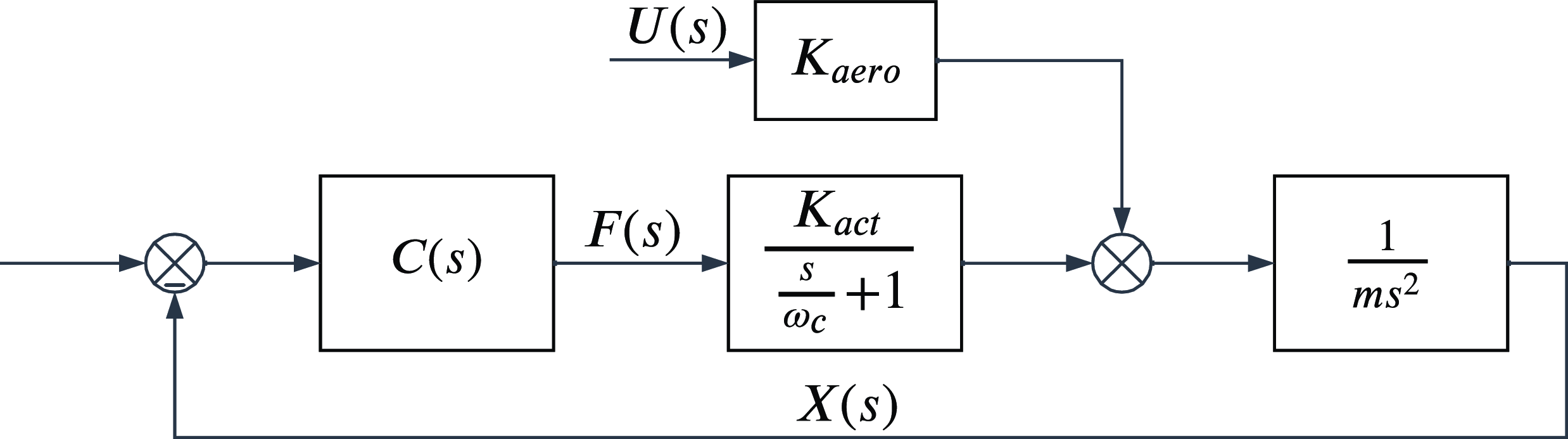


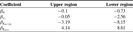

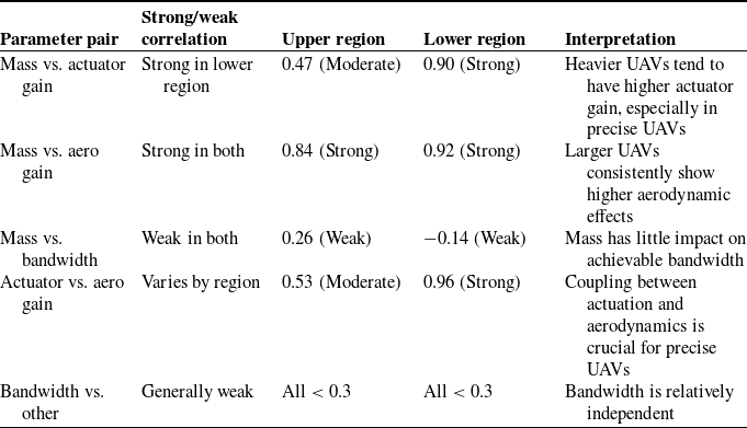

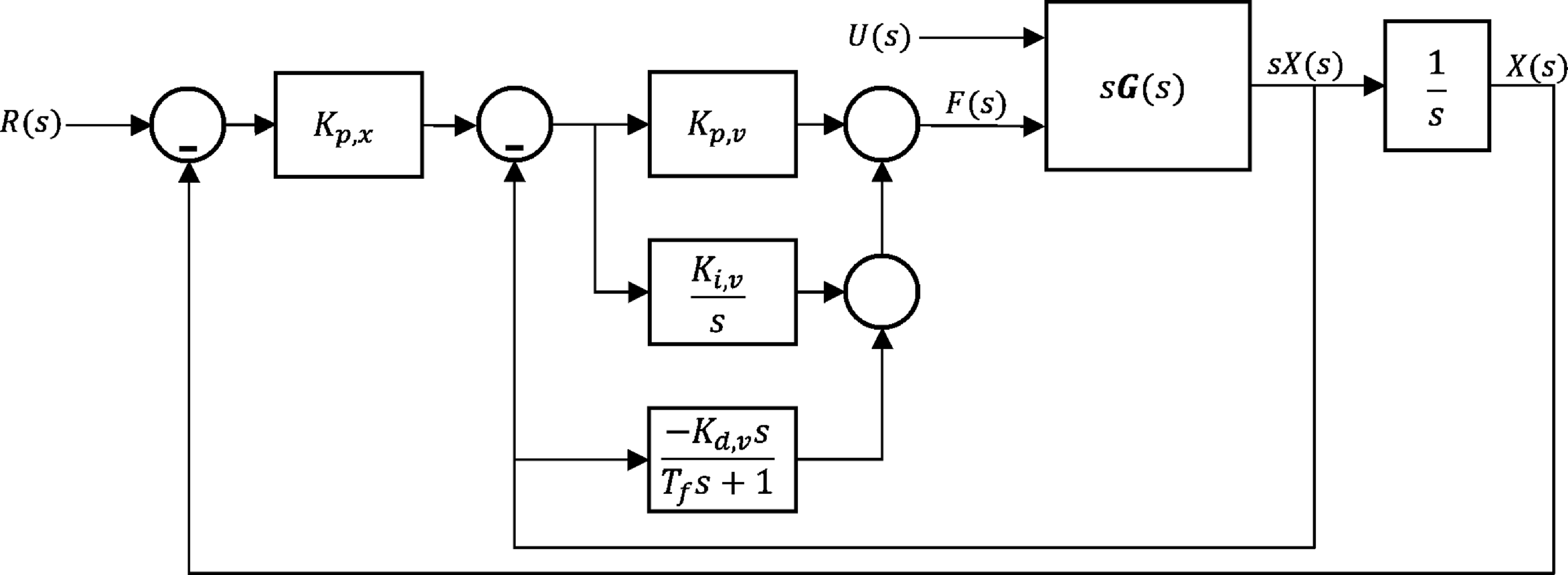


 Open access