


1. Introduction
A contact line, within the limits of the continuum approximation, is the intersection between a liquid interface and a solid, and it separates the dry region of the solid from the wet. A contact line can be static or dynamic depending on whether it is pinned to the solid surface or moves relative to it. Cases of moving contact lines are ubiquitous in nature. The motion, or the spreading, of drops on a surface, movement of a meniscus inside a tube and dipping of a solid surface into a liquid are a few examples involving this phenomenon. An understanding of the flow near a moving contact line finds importance in many industrial processes like paint coating, oil recovery, ink-jet printing and chemical etching of surfaces, to name a few. The angle that the moving liquid boundary makes with the solid (within the liquid phase) is known as the dynamic contact angle – denoted here by  $\alpha$ – and is different in magnitude from its stationary counterpart $\alpha _s$. These dynamic contact angles could be advancing ( $\alpha _a$) or receding ( $\alpha _r$), depending respectively on whether the contact line wets or de-wets the solid surface. Because the solid phase resists wetting, $\alpha _a$ are generally obtuse and are larger than $\alpha _r$. It has been observed that the dynamic contact angles depend on the capillary number $\mathit {Ca} = \mu |U|/ \gamma$, where $\mu$ is the dynamic viscosity of the liquid, $U$ is the velocity of the moving contact line and $\gamma$ is the liquid surface tension. To describe this relation, many contact line models – which are all surprisingly polynomial relations between $\alpha$ and $\mathit {Ca}$ – such as the de Gennes (de Gennes Reference de Gennes1985), Cox–Voinov (Voinov Reference Voinov1976; Cox Reference Cox1986) and even a simple linear relation (Blake & Ruschak Reference Blake and Ruschak1997) have been developed. All these models have been seen to agree well with experiments, and none can be instructively chosen over the other (Le Grand, Daerr & Limat Reference Le Grand, Daerr and Limat2005).
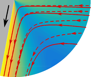
At low speeds, a moving contact line remains straight. In such cases, the flow near the contact line during the wetting or dewetting process is essentially two-dimensional. Then, the liquid and the solid interfaces would effectively form a wedge, with the contact line at the corner, as shown in figure 1. The viscous stresses within the wedge have been shown to scale as  $1/r$, where $r$ is the radial distance from the contact line (Huh & Scriven Reference Huh and Scriven1971). Note that the stress diverges at $r=0$, i.e. at the contact line, and to prevent this, it needs to be balanced either by an equivalent external pressure that maintains the flat liquid interface, or by having a deformable liquid interface that compensates with the capillary pressure from an infinite curvature (Huh & Scriven Reference Huh and Scriven1971; Shikhmurzaev Reference Shikhmurzaev2008). In the latter case, for very small capillary numbers ( $\mathit {Ca} \ll 1$), the curvature of the deformed interface is negligible except at extremely small distances from the contact line. Thus, it is reasonable to assume the liquid interface to be flat, and then model the region near the contact line as a rigid–free wedge, where the flow is forced by the relative motion of the solid. Many other mechanisms have also been proposed to balance the stress singularity at the contact line (see Dussan Reference Dussan1979; Shikhmurzaev Reference Shikhmurzaev2008; Bonn et al. Reference Bonn, Eggers, Indekeu, Meunier and Rolley2009; Snoeijer & Andreotti Reference Snoeijer and Andreotti2013, and the references therein). A commonly suggested method to overcome the tangential stress singularity is to introduce a region of perfect slip on the solid surface in close proximity of the contact line (Huh & Scriven Reference Huh and Scriven1971; Dussan Reference Dussan1976). The flow fields in such slip models render the free surface to be non-materialistic, i.e. a particle at the interface never reaches the contact line because of its zero velocity; the contact line effectively behaves as an obstacle to the flow (Shikhmurzaev Reference Shikhmurzaev2008). Experiments, however, suggest otherwise, where a rolling motion is observed, with the fluid being accelerated near the contact line (Dussan & Davis Reference Dussan and Davis1974; Chen, Ramé & Garoff Reference Chen, Ramé and Garoff1996).
Schematic of the polar coordinate system used for analysing the moving contact line problem. The contact line is at the point  $O$. The liquid interface is at $\theta =0$ and the solid surface is at $\theta =-\alpha$, where $\alpha$ is the contact angle. Here, the velocity of the solid, $U>0$ represents an advancing contact line, and $U<0$ a receding contact line. Streamlines are shown by constant $\psi$.

At sufficient proximity to the contact line, the flow is dominated by viscous forces, and it is reasonable to make the assumption of a Stokes flow. The streamfunction for the Stokes flow within a generic two-phase wedge was provided by Moffatt (Reference Moffatt1964a), which included specific cases where the boundaries moved relative to each other. For a moving three-phase contact line, Huh & Scriven (Reference Huh and Scriven1971) analysed the flow dynamics on both sides of the fluid–liquid interface, identifying self-similar feature of the flow field and highlighted the significant influence of even a thin film of the slender phase on the interface velocity and viscous dissipation. The case of flow between stationary boundaries of flat plates, i.e. a rigid–rigid wedge with homogeneous boundary conditions, where the flow originates from far-field disturbances, was carried out by Lugt & Schwiderski (Reference Lugt and Schwiderski1965), and later extended to include the dynamics of two fluids by Anderson & Davis (Reference Anderson and Davis1993). In the case of disturbance flow between stationary solid boundaries, the flow near the corner exhibited an interesting feature: the presence of an infinite sequence of eddies which decay in strength towards the corner (Moffatt Reference Moffatt1964a,Reference Moffattb; Taneda Reference Taneda1979). The presence of these eddies have also been predicted for three-dimensional flows near a conical trench (Shankar Reference Shankar1998; Sano & Hashimoto Reference Sano and Hashimoto1980).
There is no intrinsic length scale for the moving contact line problem. One can, however, define a characteristic length  $\nu /|U|$ at which the inertial and viscous dissipation are equal in magnitude; here $\nu$ is the kinematic viscosity of the liquid. The dimensionless distance is hence defined by the local Reynolds number $\rho = r/(\nu /|U|)$. Close to the contact line, where $\rho \ll 1$, the assumption of Stokes flow is perfectly valid. However, when the value of $\rho$ is appreciably large, the Stokes solution will not be sufficient to describe the flow accurately. Hence, in the case of fast motion of liquids over surfaces, like in the case of fast motion of drops studied by Puthenveettil, Senthilkumar & Hopfinger (Reference Puthenveettil, Senthilkumar and Hopfinger2013), inertia is expected to influence the flow dynamics significantly. Previous experimental and numerical studies have also looked at the influence of inertia on the apparent dynamic contact angles and flow field of a moving contact line at the scale of the physical phenomenon (Sui & Spelt Reference Sui and Spelt2013; Stoev, Ramé & Garoff Reference Stoev, Ramé and Garoff1999; Savelski et al. Reference Savelski, Shetty, Kolb and Cerro1995; Fuentes & Cerro Reference Fuentes and Cerro2007). However, a coherent analytical description of the influence of inertia, extending from the viscous (typically sub-microscopic) to the visco-inertial regime of a moving contact line, is yet unavailable. In this article, we analytically determine the inertial corrections to the Stokes flow near a steadily moving contact line. Finding such inertia-corrected flow field near a rapidly moving contact line is also important to answer the still unresolved question of whether inertia affects the dynamic contact angles (Limat Reference Limat2014).
Inertial corrections to Stokes flow near a corner have so far been available only for the case of a rigid–rigid wedge by Hancock, Lewis & Moffatt (Reference Hancock, Lewis and Moffatt1981), who considered the similarity solutions of the streamfunction as an infinite perturbation series in powers of  $\rho$, with each term of the series being an inertial correction to the previous. The dominant inertial correction term in their analysis contained a singularity at a critical corner angle $\alpha ={\rm \pi}$. Such singularities are not uncommon in other self-similar solutions of the biharmonic equation near corners, in problems of fluid mechanics and elasticity (Williams Reference Williams1952; Sternberg & Koiteri Reference Sternberg and Koiteri1958; Moffatt & Duffy Reference Moffatt and Duffy1980; Dempsey Reference Dempsey1981). The singularities are, however, spurious, and have been resolved on a case-by-case basis by determining modified expansions, often involving power-logarithmic terms, at the critical corner angle specific to the problem. In the case of flow in a rigid–rigid wedge considered by Hancock et al. (Reference Hancock, Lewis and Moffatt1981), the singularity at $\alpha ={\rm \pi}$ was nullified by an appropriate choice of the eigenfunction terms that arise from the homogeneous boundary value problem. However, the question of existence and resolution of singularities in a rigid–free wedge is still open and shall also be explored in this article.
In the present work, we provide a theoretical analysis of the effect of inertia on the hydrodynamic flow fields near a fast-moving contact line where the flow is still dominated by viscosity. To this end, we provide a locally self-similar inertial correction to the streamfunction for Stokes flow. We assume a flat liquid interface, which is a first approximation in the limit of very small capillary number ( $\mathit {Ca} \ll 1$), as discussed earlier. We strictly adhere to the no-slip boundary condition on the entirety of the solid surface as this allows us to make unbiased prediction of the influence of inertia at the length scales $l$ associated with the different contact line models.
The paper is organised as follows. After recapitulating the well-known similarity solution for Stokes flow in § 2, we obtain the inertial-correction streamfunctions in § 3. This is done by perturbing the Stokes flow streamfunction with the local Reynolds number, and then iteratively solving for the higher-order terms – which are the inertial corrections – in the Navier–Stokes equations. The homogeneous solution to the Stokes flow problem, i.e. flow between stationary boundaries due to far-field disturbances, are eigenfunctions, and are determined in § 4. In particular, we assume the disturbance flow to originate due to stick slip on the solid surface far away from the contact line. In § 5, we show that the leading-order inertial correction term is singular at a critical contact angle,  $\alpha =0.715 {\rm \pi}$. Similar to the case of rigid–rigid corner described earlier, this mathematical singularity is also resolved using the eigenfunction solutions. The resulting singularity-free, inertia-corrected flow fields are discussed in § 6.1. Inertial effects on the free-surface velocity for both advancing and receding contact lines are then discussed in detail in § 6.2, with a small-angle approximation provided in § 6.2.1. Finally, the influence of inertia on the contact angles is studied by looking at the leading-order inertial correction for the Cox–Voinov model in § 6.3, before concluding in § 7.
2. Stokes flow near a moving contact line
Consider the case of a moving contact line formed by the relative motion of a flat liquid interface over a rigid solid. The free surface of the liquid would then form a wedge with the solid surface, with the contact line at the corner, as shown in figure 1. The flow near the contact line can then be approximated as a two-dimensional flow in the rigid–free wedge (Moffatt Reference Moffatt1964a; Huh & Scriven Reference Huh and Scriven1971; Anderson & Davis Reference Anderson and Davis1993). We consider a frame of reference that is centred at the contact line. The solid surface thus moves relative to it with a velocity  $U$. A positive value of $U$ indicates an advancing contact line, and likewise, a negative value indicates a receding contact line. We shall use $U$ as the characteristic velocity for the present problem. The dynamic contact angle is denoted here by $\alpha$. As mentioned in the previous section, we define the dimensionless distance from the contact line in terms of the local Reynolds number of the flow, $\rho = r|U|/\nu$. For flows close to the contact line, $\rho \ll 1$, and the Stokes approximation holds well.
The dimensionless streamfunction for Stokes flow  $\psi_1$, non-dimensionalised by $\nu$, obeys the two-dimensional (2-D) biharmonic equation
 \begin{equation} \nabla^4 \psi_1(\rho,\theta) = 0, \end{equation}
with  $\nabla ^2=1/\rho \, \partial /\partial \rho + \partial ^2/\partial \rho ^2 + 1/\rho ^2 \partial ^2/\partial \theta ^2$. Equation (2.1) admits a general solution of the form $\psi _1 = \rho ^n f_n(\theta )$, where $n$ is any real number. For bounded velocity at the contact line ( $\rho =0$), we have the condition $n \geqslant 1$. The exact value of $n$ is determined from the relevant boundary conditions for the problem. In the present case, the boundary conditions are: no slip at the solid surface,
 \begin{equation} \left.-\frac{\partial \psi_1}{\partial \rho}\right|_{\theta={-}\alpha} = 0 \quad \mbox{and} \quad \left.\frac{1}{\rho} \frac{\partial \psi_1}{\partial \theta}\right|_{\theta={-}\alpha} ={\pm} 1, \end{equation}
no-penetration and zero-shear-stress conditions on the free surface, given respectively by
 \begin{equation} \left.-\frac{\partial \psi_1}{\partial \rho}\right|_{\theta=0} =0 \quad \mbox{and} \quad \left.\left(-\frac{\partial^2 \psi_1}{\partial \rho^2}+\frac{1}{\rho^2}\frac{\partial^2 \psi_1}{\partial \theta^2}+\frac{1}{\rho} \frac{\partial \psi_1}{\partial \rho}\right)\right|_{\theta=0}=0. \end{equation}
Note that in the above equations, the velocities were made dimensionless using the characteristic velocity,  $|U|$. The positive value in the right-hand side of (2.2a,b) is used when it is an advancing contact line while the negative value is used in case of a receding contact line. The form of the boundary conditions (2.2a,b)–(2.3a,b) suggest a self-similar solution of the form (Moffatt Reference Moffatt1964a; Moffatt & Duffy Reference Moffatt and Duffy1980; Batchelor Reference Batchelor2000)
 \begin{equation} \psi_1(\rho,\theta) = \rho f_1(\theta). \end{equation}
Substituting (2.4) in the governing biharmonic equation (2.1) gives
 \begin{equation} f_{1}(\theta)+2\,f_{1}''(\theta)+f_{1}^{\prime\prime\prime\prime}(\theta) =0, \end{equation}
where each  $'$ denotes the derivative of the function. Solving for $f_1(\theta )$ gives the general form of the function as (Moffatt Reference Moffatt1964a; Leal Reference Leal2007)
 \begin{equation} f_1(\theta)= A \cos\theta+ B \sin\theta + C \theta \cos\theta + D \theta \sin\theta. \end{equation}
The coefficients  $A$,
$A$,  $B$,
$B$,  $C$ and $D$ are to be determined from the boundary conditions of the problem. Replacing $f_1(\theta )$ in (2.4) with the expression derived in (2.6), and subsequently using it in the boundary conditions, (2.2a,b) and (2.3a,b), gives the coefficients, which are functions of $\alpha$, as (Moffatt Reference Moffatt1964a; Leal Reference Leal2007)
 \begin{equation} A=0,\quad B(\alpha) ={\pm} \frac{2 \alpha \cos\alpha} {2\alpha-\sin2\alpha},\quad C(\alpha) ={\mp} \frac{2\sin\alpha}{2\alpha-\sin 2\alpha},\quad \text{and} \quad D = 0. \end{equation}
The signs  $(\pm )$ of $B$ and $C$ depend on the whether the contact line is advancing or receding, respectively. Using (2.6) and (2.7a–d), the streamfunction for Stokes flow (2.4) becomes
 \begin{equation} \psi_1(\rho,\theta) = \rho f_1(\theta) ={\pm} \frac{\rho(2 \alpha \cos \alpha \sin\theta - 2\theta \cos\theta \sin \alpha )}{2\alpha - \sin 2\alpha}. \end{equation}
3. Inertial corrections to the Stokes flow
The exact solution of the flow field is described by the 2-D steady Navier–Stokes equation, written in streamfunction form as
 \begin{equation} \nabla^4 \psi = \frac{1}{\rho}\left( \frac{\partial {\psi}}{\partial{\theta}}\, \frac{\partial(\nabla^2 \psi)}{\partial \rho} - \frac{\partial \psi}{\partial \rho} \, \frac{\partial (\nabla^2 \psi)}{\partial \theta} \right). \end{equation}
The terms in the left- and the right-hand sides of (3.1) represent the viscous and the inertial dissipation, respectively. In the case of Stokes flow, one can neglect the right-hand side to recover the biharmonic equation (2.1). The Navier–Stokes equation (3.1) is linear in its highest-order derivatives, and so, its exact solution can be constructed in a linear fashion by writing it as a series expansion of the fundamental Stokes solutions. Thus, it is possible to construct the streamfunction  $\psi$ in (3.1) as a Taylor series expansion in terms of the local Reynolds number $\rho$, of the form
 \begin{equation} \psi(\rho,\theta) = \sum_{n=1}^\infty \psi_n (\rho,\theta) \quad \mathrm{where}\ \psi_{n}(\rho,\theta)=\rho^{n} \, f_{n}(\theta), \end{equation}
which converges when  $\rho \ll 1$ (Lugt & Schwiderski Reference Lugt and Schwiderski1965; Hancock et al. Reference Hancock, Lewis and Moffatt1981; Batchelor Reference Batchelor2000). The self-consistency of the expression in (3.2) can be justified by noting that when it is applied in (3.1), the viscous terms are $O(\rho ^{n-4})$ while the inertial terms are of much smaller strength $O(\rho ^{2n-4})$. Thus, each successive term in the series (3.2) can be regarded as an inertial correction to the previous (Hancock et al. Reference Hancock, Lewis and Moffatt1981; Fuentes & Cerro Reference Fuentes and Cerro2007). We now use (3.2) in (3.1), and collect terms of the same order of magnitude in $\rho ^n$. At the leading order, when $n=1$, we get back the ordinary differential equation for $f_1(\theta )$ in (2.5), i.e. we retrieve the solution in the Stokes limit (2.6). When $n \geqslant 2$, we can write a general expression of the resulting ordinary differential equation as
 \begin{align} &\left(\frac{\textrm{d}^2}{\textrm{d} \theta^2} + n^2\right) \left(\frac{\textrm{d}^2}{\textrm{d} \theta^2} + (n-2)^2 \right) f_n(\theta) \nonumber\\ &\quad = \sum_{i+j=n} \left((j-2) f'_i(\theta) - i f_i(\theta) \frac{\textrm{d}}{\textrm{d} \theta}\right) \left(\frac{\textrm{d}^2}{\textrm{d} \theta^2} + j^2\right) f_j(\theta), \end{align}
which can be solved for iteratively. When we use  $n=2$ in (3.3) we get
 \begin{equation} 4\,f_{2}''(\theta)+f_{2}^{\prime\prime\prime\prime}(\theta)={-}2\,f_{1}(\theta) f_{1}'(\theta) - f_{1}' (\theta) f_{1}''(\theta) - f_{1}(\theta) f_{1}'''(\theta). \end{equation}
Substituting  $f_{1}(\theta )$ from (2.6) in (3.4), and solving for $f_2(\theta )$, we get the first inertial-correction term $\psi _2=\rho ^2 f_2(\theta )$, with
 \begin{equation} f_{2}(\theta)= P+Q\theta+R\cos2\theta+S\sin2\theta+ E\theta\cos2\theta + H\theta^2\sin2\theta. \end{equation}
The coefficients in (3.5), in their functional form, are
 \begin{equation} E(\alpha) =\frac{4 B(\alpha) C(\alpha) - 3 C(\alpha)^2}{32},\quad \textrm{and} \quad H(\alpha) =\frac{-C(\alpha)^2}{16}, \end{equation}
with  $B$ and $C$ given in (2.7a–d). Expressions for $P$,
$P$,  $Q$,
$Q$,  $R$ and $S$ can be obtained from the velocity and free-shear boundary conditions at this order of magnitude, $O(\rho )$. The no-slip condition on the solid surface gives
 \begin{equation} \left.-\frac{\partial \psi_2}{\partial \rho}\right|_{\theta={-}\alpha} =0 \implies f_{2}(-\alpha) = 0 \end{equation}
and
 \begin{equation} \left.\frac{1}{\rho} \frac{\partial \psi_2}{\partial \theta}\right|_{\theta={-}\alpha} = 0 \implies f_{2}'(-\alpha) = 0. \end{equation}
Note that the solid has a constant dimensionless velocity  $\pm 1$, and has no perturbation of the order of magnitude of the inertial correction, $O(\rho )$. The no-penetration condition, i.e. zero normal velocity on the free surface gives
 \begin{equation} \left.-\frac{\partial \psi_2}{\partial \rho}\right|_{\theta=0} =0 \implies f_{2}(0) = 0. \end{equation}
The zero-shear-stress boundary condition on the free surface gives
 \begin{equation} \left.\left(-\frac{\partial^2 \psi_2}{\partial \rho^2}+\frac{1}{\rho^2}\frac{\partial^2 \psi_2}{\partial \theta^2}+\frac{1}{\rho} \frac{\partial \psi_2}{\partial \rho}\right)\right|_{\theta=0}=0 \implies f_{2}''(0)- f_{2}(0)=0. \end{equation}
Applying the boundary conditions (3.9) and (3.10) in (3.5) gives  $P=0$ and $R=0$. Then, applying the no-slip boundary conditions of (3.7) and (3.8) in (3.5) gives
 \begin{equation} Q(\alpha) = \frac{M(\alpha) \sin2\alpha}{2\alpha\cos2\alpha - \sin2\alpha} \quad \mbox{and} \quad S(\alpha) = S_1(\alpha)+ S_2(\alpha), \end{equation}
where
 \begin{equation} S_{1}(\alpha) =\frac{- \alpha M(\alpha)}{2\alpha\cos2\alpha - \sin2\alpha} \quad \mbox{and} \quad S_{2}(\alpha) = \frac{-E(\alpha)\alpha\cos2\alpha - H(\alpha)\alpha^{2} \sin2\alpha}{\sin 2\alpha}, \end{equation}
with  $M(\alpha )$ given by
 \begin{equation} M(\alpha) = ({-}2\alpha\sin2\alpha + \cos2\alpha) E(\alpha) + (2\alpha^{2}\cos2\alpha + 2\alpha\sin2\alpha)H(\alpha)+ 2S_{2}(\alpha) \cos2\alpha. \end{equation}
The factorisation  $S= S_1+S_2$ in (3.11a,b) was performed in order to collect terms of the common denominators together. Finally, substituting the coefficients from (3.6a,b), (3.11a,b) and (3.12a,b) in (3.5), and simplifying yields
 \begin{equation} f_{2}(\theta) = \frac{S_1(\alpha)}{\alpha} \left(\alpha \sin2\theta - \theta \sin2\alpha \right) + E(\alpha) \theta \cos2\theta + H(\alpha) \theta^{2} \sin{2\theta} + S_{2}(\alpha) \sin2\theta. \end{equation}
The dimensionless streamfunction of the leading-order inertial correction is then obtained by using (3.14) in (3.2), for  $n=2$, as
 \begin{align} \psi_{2}(\rho,\theta) = \rho^2\;f_2(\theta) &= \rho^2\left( \frac{S_1(\alpha)}{\alpha}\left(\alpha \sin2\theta - \theta \sin2\alpha\right) \right. \nonumber\\ &\quad\left. +\, E(\alpha) \theta \cos2\theta + H(\alpha) \theta^{2} \sin{2\theta} + S_{2}(\alpha) \sin2\theta \vphantom{\frac{S_1(\alpha)}{\alpha}}\right). \end{align}
Thus, the dimensionless streamfunction (3.2), comprising of only the Stokes and the dominant inertial-correction terms, is  $\psi =\psi _1+\psi _2,$ where $\psi _1$, given in (2.8), is the Stokes term and $\psi _2$, given in (3.15), is the leading-order inertial correction.
4. Contribution from the eigenfunctions
The solution of the biharmonic equation, i.e. the streamfunction for Stokes flow (2.8), satisfies the boundary conditions in the Stokes limit, but is, however, incomplete. It requires to be supplemented with the general solution that satisfies the homogeneous boundary conditions (Hancock et al. Reference Hancock, Lewis and Moffatt1981). Physically, such eigenfunction solutions represent Stokes flows near a stationary corner, created by disturbances that originate far away from it. These ‘disturbance’ flows are generally expressed as a combination of all the possible asymmetric and symmetric flows near the corner (Moffatt Reference Moffatt1964a; Lugt & Schwiderski Reference Lugt and Schwiderski1965). They are not commonly included in the Stokes solution (2.8) because their relative contribution to the flow field is asymptotically negligible in comparison. However, compared with the inertial-correction terms, their contributions are not negligible (Hancock et al. Reference Hancock, Lewis and Moffatt1981). The dimensionless streamfunction for such disturbance flows, with  $\rho \ll 1$, is given by the series (Moffatt Reference Moffatt1964a; Hancock et al. Reference Hancock, Lewis and Moffatt1981)
 \begin{equation} \psi_{e}(\rho,\theta) = \textrm{Re} \left( \sum_{m=1}^\infty \psi_{e_m}(\rho,\theta) \right) \quad \mathrm{with} \ \psi_{e_m}(\rho,\theta) = A_{m} \rho^{\lambda_{m}} g_{m}(\theta), \end{equation}
where  $A_{m}$ are arbitrary constants, and the complex eigenvalues $\lambda _{m}$ are such that $1<\textrm {Re}(\lambda _{1})\leqslant \textrm {Re}(\lambda _{2})\leqslant \ldots$ with $\textrm {Re}$ indicating the real part. The corresponding eigenfunctions $g_{m}(\theta )$ have the well-known form (Moffatt Reference Moffatt1964a; Hancock et al. Reference Hancock, Lewis and Moffatt1981; Anderson & Davis Reference Anderson and Davis1993; Shankar Reference Shankar1998)
 \begin{equation} g_m(\theta) = \sin\lambda_{m}\theta \sin(\lambda_{m}-2)\alpha - \sin\lambda_{m}\alpha \sin(\lambda_{m}-2)\theta, \quad \textrm{where}\ \lambda_m \neq 2. \end{equation}
We shall discuss the special case of  $\lambda _m= 2$ in § 5.1. Equation (4.2) corresponds to symmetric flows between two rigid plates at $\theta =\pm \alpha$ and hence satisfies free-shear condition along $\theta = 0$, i.e. the liquid interface in our problem; the asymmetric modes, however, do not meet the no-penetration condition at $\theta = 0$ and are hence discarded here (cf. Anderson & Davis Reference Anderson and Davis1993). The eigenvalues, $\lambda _m$, are determined by applying the homogeneous boundary conditions on $g_m(\theta )$ in (4.2). Thus, using
 \begin{equation} g_m(0) =0, \quad g_m''(0)-g_m(0) =0 \end{equation}
and
 \begin{equation} g_m(-\alpha) = 0,\quad g_m'(-\alpha) =0, \end{equation}
one can show that the eigenvalues form the roots of a function (Dean & Montagnon Reference Dean and Montagnon1949; Williams Reference Williams1952; Moffatt Reference Moffatt1964a; Moffatt & Duffy Reference Moffatt and Duffy1980)
 \begin{equation} W(\lambda)=\sin (2(\lambda-1)\alpha) - (\lambda-1)\sin 2\alpha, \end{equation}
i.e.  $W(\lambda _m) = 0$. The real and imaginary parts of the first few roots are plotted in figure 2. It can be seen in figure 2 that for $\alpha < \alpha _1 = 0.442 {\rm \pi}$, all the roots $\lambda _m$, with $m \geqslant 1$, are complex. The complex nature of the eigenvalues have been shown to physically imply the presence of an infinite sequence of eddies near the stationary corner (Moffatt Reference Moffatt1964a; Taneda Reference Taneda1979).
Variation of the real (solid lines) and imaginary (dashed lines) parts of the complex eigenvalues  $\lambda _1$, $\lambda _2$ and $\lambda _3$ with the contact angle. Circle markers show the locations of double roots of the function $W(\lambda )$. The triangular marker shows $\lambda _1 = 2$ at $\alpha =\alpha _0 = 0.715{\rm \pi}$. Note especially that $\lambda _1$ is real when $\alpha \geqslant \alpha _1$; $\lambda _2$ is real when $\alpha _1 \leqslant \alpha \leqslant \alpha _2$ and $\alpha \geqslant \alpha _3$.

Next, an expression for the arbitrary constant  $A_m$ in (4.1) could have been obtained using the property of biorthogonality of eigenfunctions if the far-field boundary conditions were specified (Liu & Joseph Reference Liu and Joseph1978; Shankar Reference Shankar2003). But, since they are unknown in the present problem, we resort to modelling this as a disturbance flow created by a stick slip at the solid surface far from the contact line (see Appendix A for details). This is a natural assumption for the origin of disturbance flows, as every surface contains inhomogeneities such as geometrical irregularities, or regions of impurities like lubricants or entrapped air which can act as local regions of slip (de Gennes Reference de Gennes1985; Cox Reference Cox1983; David & Neumann Reference David and Neumann2010; Sui, Ding & Spelt Reference Sui, Ding and Spelt2014). Entrapped microscopic bubbles are observed especially in fast-moving contact lines, both in simulations and experiments (Marchand et al. Reference Marchand, Chan, Snoeijer and Andreotti2012; Chan et al. Reference Chan, Srivastava, Marchand, Andreotti, Biferale, Toschi and Snoeijer2013; Jian et al. Reference Jian, Josserand, Popinet, Ray and Zaleski2018). Here, we find that the streamfunction of the disturbance flow created by a region of slip far from the contact line, given in (A13), is indeed identical to the general expression given in (4.1). Therefore, comparing these two equations gives the expression of the coefficient $A_m$ as
 \begin{equation} A_m = \frac{C^{{\lambda_m}-1}_m}{({\lambda_m}-1)W'(\lambda_m)}, \end{equation}
where  $W'(\lambda )$ is the derivative of (4.5), given in (A11), and $C_m$ is a coefficient which is yet to be determined. Using (4.2) and (4.6) in (4.1), the expression for the eigenfunction terms is finally obtained as
 \begin{equation} \psi_{e_m} (\rho,\theta) = \frac{C^{{\lambda_m}-1}_m \rho^{\lambda_m} (\sin{(\lambda_m-2) \alpha} \sin {\lambda_m \theta} -\sin {\lambda_m \alpha} \sin{(\lambda_m-2) \theta})}{({\lambda_m}-1)(2\alpha\cos(2({\lambda_m}-1)\alpha) - \sin 2\alpha)}. \end{equation}
An expression of the form in (4.7) is commonly seen in stationary corner flow problems such as forced corner flows and Jeffery–Hamel problem (Moffatt & Duffy Reference Moffatt and Duffy1980). The choice of  $C_m$ is, however, still arbitrary at the moment, but we shall see in § 5 how this apparent freedom allows for a proper choice that eliminates some spurious singularities that arise in the streamfunction solution.
The complete streamfunction, which satisfies the Navier–Stokes equation, is now obtained by combining the Stokes solution (2.8), the inertial correction (3.2) and the eigenfunction solutions (4.1) as
 \begin{equation} \varPsi (\rho,\theta) = \psi (\rho,\theta) + \psi_e (\rho,\theta)= \sum_{n=1}^\infty \psi_n (\rho,\theta)+\textrm{Re} \left(\sum_{m=1}^\infty \psi_{e_m}(\rho,\theta) \right). \end{equation}
Rewriting the terms in (4.8) using (3.2) and (4.1) gives
 \begin{equation} \varPsi (\rho,\theta) = \sum_{n=1}^\infty \rho^{n} \, f_{n}(\theta) + \textrm{Re} \left(\sum_{m=1}^\infty A_{m} \rho^{\lambda_{m}} g_{m}(\theta)\right). \end{equation}
By comparing the order of magnitude of the terms in (4.9) when  $\rho \ll 1$, it can be seen that the first N terms of $\psi$ dominate over $\psi _{e_m}$ only when $N<\textrm {Re} (\lambda _m) \leqslant N+1$. This would imply that, when $\textrm {Re}(\lambda _1) \leqslant 3$, which corresponds to $\alpha \geqslant 0.5 {\rm \pi}$ (see figure 2), the first eigenfunction term $\psi _{e_1}$, of $O(\rho ^{\lambda _1})$, is non-negligible compared with the leading-order inertial correction $\psi _2$ which is of $O(\rho ^2)$, and should not be discarded. Nonetheless, as long as $\alpha < 0.715 {\rm \pi}$ ( $=\alpha _0$; see figure 2), we have $\lambda _m > 2$, and so all eigenfunctions $\psi _{e_m}$ are subdominant compared with $\psi _2$ . However, when $\alpha =\alpha _0$, $\lambda _1=2$ and the eigenfunction $\psi _{e_1}$ is of the same order of magnitude as $\psi _2$. For values of $\alpha \geqslant \alpha _0$, $\psi _{e_1}$ dominates over all the inertial-correction terms; the principal correction to the Stokes solution, in this case, is from the first eigenfunction term, i.e. the Stokes flows are influenced primarily by the disturbance flows rather than inertia. Note from figure 2 that the first eigenvalue, $\lambda _1$, is always greater than 1 within $\alpha \leqslant {\rm \pi}$ (Lugt & Schwiderski Reference Lugt and Schwiderski1965). This makes the corresponding leading-order eigenfunction $\psi _{e_1}$, and hence all the eigenfunction terms, subdominant compared with the streamfunction for Stokes flow, $\psi _1$ in the expansion (4.9). This means that the Moffatt eddies, which are created by the disturbance flows, are suppressed by the dominant Stokes flow in a moving contact line that satisfies the no-slip boundary conditions. On the contrary, when using a slip boundary condition near a moving contact line, these eddies have been found to have significant influence on the Stokes flow (Kirkinis & Davis Reference Kirkinis and Davis2014).
For the present analysis, we limit the influence of inertial correction to the leading-order alone. Thus, we truncate the complete streamfunction expansion (4.8) beyond the first few leading-order terms, i.e.
 \begin{equation} \varPsi \approx \psi_{1}+ \psi_{2} + \textrm{Re} (\psi_{e_1}+ \psi_{e_2}), \end{equation}
where  $\psi _1$ is the Stokes solution (2.8), $\psi _2$ the leading-order inertial correction (3.15), and $\psi _{e_1}$ and $\psi _{e_2}$, given by (4.7) for $m=1$ and $2$ respectively, are the first and second eigenfunctions. Note that $\psi _{e_2}$ has also been included here because it is of the same order of magnitude as $\psi _{e_1}$ when $\alpha \leqslant \alpha _1 = 0.442 {\rm \pi}$, as their eigenvalues are equal in this domain, as seen in figure 2. However, by this argument, $\psi _{e_3}$ (and by extension, all higher-order terms) also needs to be included, as there is also a region $0.55 {\rm \pi}< \alpha < 0.91 {\rm \pi}$ where the eigenvalues $\lambda _2$ and $\lambda _3$ are equal. Nonetheless, we have chosen to neglect its contribution, as all the higher-order terms are anyway insignificant compared with the leading-order term $\psi _{e_1}$ when $\alpha > 0.5 {\rm \pi}$.
5. Singularities in the streamfunctions and their resolution
The leading-order inertial correction,  $\psi _2$ in (3.15) is seen to diverge to infinity when $\alpha = \alpha _0 = 0.715 {\rm \pi}$ because $\alpha _0$ is a root of the denominator of one of its coefficients, $S_1$ (in (3.12a,b)). In other words, $\psi _2$ is singular because
 \begin{equation} 2 \alpha_0 \cos 2\alpha_0 -\sin2\alpha_0 =0. \end{equation}
In fact, the streamfunction expansion in (3.2), and hence  $\varPsi$ in (4.10), becomes incorrect even when $\alpha \neq \alpha _0$ if the asymptotic series, with $\rho \ll 1$, is non-uniform, i.e. when $S_1$ is of the order of magnitude of $1/\rho$. Similar singularities have been previously reported in solutions of the biharmonic equation in problems of fluid flows and elasticity, and each of them have been resolved individually, either analytically or numerically (see Sternberg & Koiteri Reference Sternberg and Koiteri1958; Moffatt & Duffy Reference Moffatt and Duffy1980). Following the approach of Hancock et al. (Reference Hancock, Lewis and Moffatt1981), we propose to resolve the described singularity in $\psi _2$ by making an appropriate choice of the coefficient $C_1$ in the first eigenfunction $\psi _{e_1}$ in (4.7) so that the singular terms in $\psi _2$ are nullified by $\psi _{e_1}$ when they are evaluated in unison.
5.1. Solution at the critical angle  $\alpha =\alpha _0$

Let the contact angle  $\alpha$ be in close neighbourhood of $\alpha _{0}$, i.e. $\alpha =\alpha _{0}\pm \varepsilon$, with $\varepsilon \to 0$. The leading-order inertial-correction term in (3.15) then becomes
 \begin{align} \psi_{2} &= \rho^2 \left(\frac{\pm M(\alpha_0)}{4 \varepsilon \alpha_0 \sin 2\alpha_0} (\alpha_{0}\sin2\theta - \theta \sin2\alpha_{0}) + E(\alpha_0) \theta \cos 2\theta + H(\alpha_0) \theta^2 \sin 2\theta\right. \nonumber\\ &\left.\quad\vphantom{\frac{\pm M(\alpha_0)}{4 \varepsilon \alpha_0 \sin 2\alpha_0}} + S_2(\alpha_0) \sin 2\theta + O(\varepsilon) \right). \end{align}
Notice the singular term that arises in (5.2) when  $\varepsilon = 0$, i.e. when $\alpha =\alpha _0$.
In a manner similar to deriving (5.2), we shall now determine the expression for  $\psi _{e_1}(\theta )$ in the neighbourhood of $\alpha _0$. The eigenvalue $\lambda _1$ is determined after substituting $\alpha = \alpha _0 \pm \varepsilon$ in (4.5) as
 \begin{equation} \lambda_{1} \approx 2 \mp\frac{\displaystyle \varepsilon}{\displaystyle \alpha_{0}}. \end{equation}
From figure 2, note that  $\lambda _1$ does not have any complex part in the neighbourhood of $\alpha _0$. Substituting $\lambda _1$ from (5.3) in the expressions for $g_m(\theta )$ (4.2) and $A_m$ (4.6), gives, for $m=1$,
 \begin{equation} {g_{1}}(\theta)={\mp} \frac{\varepsilon}{\alpha_0}\left(\alpha_{0}\sin2\theta - \theta \sin2\alpha_{0}\right), \end{equation}
and
 \begin{equation} A_1 = \frac{{C_1}^{1\mp \varepsilon/\alpha_0}}{4\varepsilon^2(1\pm \varepsilon/\alpha_0)\sin 2\alpha_0}, \end{equation}
respectively. Note that (5.1) was used to simplify the above expressions. Finally, using (5.4) and (5.5) in the expression for the eigenfunction in (4.7) gives the first eigenfunction near the contact angle  $\alpha =\alpha _0 \pm \varepsilon$ as
 \begin{align} \textrm{Re} (\psi_{e_1}) &= \frac{\rho^{2 \mp \varepsilon/\alpha_0} C_1^{{\mp} \varepsilon/\alpha_0}}{4 \alpha_0\sin 2\alpha_0}\left({\mp} \frac{(\alpha_0 \sin 2\theta - \theta \sin 2\alpha_0)}{\varepsilon} \right.\nonumber\\ &\quad + \left. 2 \theta(\cos 2\theta + \cos 2\alpha_0)-2 \sin 2\theta) \vphantom{\left({\mp} \frac{(\alpha_0 \sin 2\theta - \theta \sin 2\alpha_0)}{\varepsilon} \right.}\right). \end{align}
Note that (5.6) is also singular at the same rate as (5.2), i.e.  $\varepsilon ^{-1}$ as $\varepsilon \to 0$. By assigning $C_1 = M(\alpha _0) \approx 0.0692$, and considering the streamfunctions $\psi _2$ and $\psi _{e_1}$ together, i.e. adding (5.2) and (5.6), we get
 \begin{align} \psi_{2} + \textrm{Re} (\psi_{e_1}) & ={\pm}\frac{\rho^2 M(\alpha_0) \left(1-(\rho\;M(\alpha_0))^{{\mp} \varepsilon/\alpha_0}\right)}{4\varepsilon\alpha_0\sin 2\alpha_0}(\alpha_0 \sin 2\theta - \theta \sin 2\alpha_0) \nonumber\\ &\quad + \rho^2 (\sin 2\theta - \theta \cos 2\alpha_0) E(\alpha_0) \nonumber\\ &\quad + \rho^2[ ((\theta^2-1) \sin 2\theta + \theta (\cos 2 \theta + \cos 2 \alpha_0)) H(\alpha_0) \nonumber\\ &\qquad \quad + S_{2}(\alpha_0) \sin2\theta]+O(\varepsilon). \end{align}
Finally, evaluating (5.7) in the limit  $\varepsilon \to 0$ gives a non-singular expression for the combined streamfunction as $\psi _{2} + \textrm {Re} (\psi _{e_1}) = \rho ^2 \ln \rho \, \tilde {f}(\theta ) + \rho ^2 \breve {f}(\theta )$, where
 \begin{gather} \tilde{f}(\theta) = \frac{(\alpha_0\sin 2\theta -\theta\sin2\alpha_0)M(\alpha_0)}{4{\alpha_0}^2\sin 2 \alpha_0}, \end{gather}
 \begin{align} \breve{f}(\theta) &= \frac{(\alpha_0\sin 2\theta -\theta\sin2\alpha_0)M(\alpha_0)}{4{\alpha_0}^2\sin 2 \alpha_0} \ln(M(\alpha_0)) + (\sin 2\theta - \theta \cos 2\alpha_0) E(\alpha_0)\nonumber\\ &\quad + [(\theta^2-1) \sin 2\theta + \theta (\cos 2 \theta + \cos 2 \alpha_0)] H(\alpha_0) + S_{2}(\alpha_0) \sin2\theta. \end{align}
Thus, we see that with this choice of  $C_1=M(\alpha _0)$, the combined function $\psi _{2} + \textrm {Re} (\psi _{e_1})$ – which exists in the complete streamfunction (4.10) – is no longer singular at the critical angle $\alpha =\alpha _0$. Moreover, note that the expression for the complete streamfunction in this case would not be the simple power series expansion of (4.9), but rather an asymptotic expansion of the form
 \begin{equation} \left.\varPsi(\rho,\theta)\right|_{\alpha=\alpha_0} = \rho f_1(\theta) + \rho^2 \ln \rho\, \tilde{f}(\theta) + \rho^2 \breve{f}(\theta) + O(\rho^3), \end{equation}
where the non-singular functions  $\tilde {f} (\theta )$ and $\breve {f}(\theta )$ are given in (5.8) and (5.9), respectively. It is interesting to note that this fixed value of $C_1 \approx 0.0692$ is quite close to the numerically obtained value of the coefficient ( $C_1=0.092$) given by Sprittles & Shikhmurzaev (Reference Sprittles and Shikhmurzaev2009) for a contact line with slip boundary condition. It may be noted that we have chosen $C_1$ to be a constant here, i.e. independent of $\alpha$, only for convenience. Nevertheless, since $\psi _2$ is dominant over all $\psi _{e_m}$ when $\alpha <\alpha _0$, no significant difference arises by choosing a different expression for $C_m$, as long as the eigenfunction does not diverge in this range of contact angles (see Appendix B, figure 10).
5.2. Additional singularities in the eigenfunctions
The coefficient  $A_m$ in (4.6), which appear in the general expression for the eigenfunctions given by (4.1), has $W'(\lambda _m)$ in its denominator. The function $W'(\lambda _m)$, given by (A11), has roots at certain contact angles, shown by $\alpha _1,\alpha _2 \ldots$ in figure 2. Thus, it might appear that the eigenfunctions are singular at these specified angles as well. For example, in the present analysis, where we take into account the contributions from the first two eigenfunction terms, $\psi _{e_1}$ and $\psi _{e_2}$, we encounter a singularity in the terms at $\alpha =\alpha _1\approx 0.442 {\rm \pi}$. However, after noting that $\lambda _1$ and $\lambda _2$ are the double poles of (4.5) with $\lambda _1=\lambda _2 = 3.78$ when $\alpha = \alpha _1$ (see figure 2), i.e. both $W(\lambda _{1,2})=0$ and $W'(\lambda _{1,2})=0$ at these contact angles, we consequently use the residual theorem to overcome these spurious singularities (see Appendix A). As derived in (A14) the correct, non-singular expression of the eigenfunctions at $\alpha =\alpha _1$ is in fact
 \begin{align} &\psi_{e_1} (= \psi_{e_2}) \nonumber\\ &\quad = \frac{\rho^{\lambda_1} C^{\lambda_1-1}_1}{4 \alpha^2_1 \sin (2(\lambda_1-1)\alpha_1)}\left[\ln(\rho C_1)\left(\sin{(\lambda_1-2) \alpha_1} \sin {\lambda_1 \theta} -\sin {\lambda_1 \alpha_1} \sin{(\lambda_1-2) \theta}\right) \right.\nonumber\\ &\qquad + \alpha_1 \left( \cos{(\lambda_1-2) \alpha_1} \sin{\lambda_1 \theta} - \cos{\lambda_1 \alpha_1} \sin{(\lambda_1-2) \theta}\right) \nonumber\\ & \qquad \left.+ \theta \left(\sin{(\lambda_1-2) \alpha_1} \cos{\lambda_1 \theta} - \sin{\lambda_1 \alpha_1} \cos{(\lambda_1-2) \theta}\right)\right], \end{align}
with  $\lambda _1 = 3.78$. As before, the arbitrary constants are chosen as $C_1= C_2 = M(\alpha _0)$. The singularity-free expression of the complete streamfunction, in this case, takes the form
 \begin{equation} \left.\varPsi(\rho,\theta)\right|_{\alpha=\alpha_1} = \rho f_1(\theta) + \rho^2 f_2(\theta) + O(\rho^3) + \rho^{3.78} \ln\rho \,\tilde{g}(\theta) + \rho^{3.78}\, \breve{g}(\theta), \end{equation}
where the functions  $\tilde {g} (\theta )$ and $\breve {g}(\theta )$ may be easily inferred from (5.11). Since $\alpha _1 < 0.5 {\rm \pi}$, the leading-order contributions from the eigenfunction terms are much smaller than the inertial-correction terms, as expected. The same procedure may be implemented to resolve singularities that occur in all of the eigenfunctions at the remaining double roots of (4.5).
At first glance, it might appear to be a happy coincidence that at the critical contact angle, the leading-order inertial term and the first eigenfunction term are of the same asymptotic order, are both singular, and their combination magically yields a non-singular, non-zero streamfunction. Botella & Peyret (Reference Botella and Peyret2001) argued the corollary, that the singularities in the streamfunctions arise because the leading-order inertial and eigenfunction terms are asymptotically of the same order of magnitude, i.e.  $O(\rho ^{\lambda _1})=O(\rho ^2)$, at this critical contact angle. These terms are then forced to simultaneously satisfy the Stokes (by eigenfunction) as well as the Navier–Stokes (by leading-order inertial term) equations, which results in singular solutions. To avoid the singularity, they suggested the use of a power-logarithmic streamfunction expansion instead, which we have re-obtained in (5.10) from first principles. Similar modified expansions of the streamfunction for other corner flow problems, at their respective critical corner angles, have also been determined previously (Moffatt & Duffy Reference Moffatt and Duffy1980; Hancock et al. Reference Hancock, Lewis and Moffatt1981; Sinclair Reference Sinclair2010; Nitsche & Bernal Reference Nitsche and Bernal2018). Some of these authors have used the power-logarithmic series as the general solution of the biharmonic equation, and have obtained the conditions under which the log terms have non-zero coefficients viz. when the eigenvalues transition from complex to real and vice-versa (see figure 2). This transition happens when the eigenvalues are integers or double roots (Dempsey & Sinclair Reference Dempsey and Sinclair1979; Botella & Peyret Reference Botella and Peyret2001; Paggi & Carpinteri Reference Paggi and Carpinteri2008). Thus, the modified expansion is reminiscent of that determined using the method of Frobenius (see for e.g. Teschl Reference Teschl2012, chapter 4). Drawing from these studies, we suspect that the power series expansion of the streamfunction in the present problem (in (4.9)) also requires modification when the eigenvalues are either (i) integers, i.e. $\lambda _m = n$, or (ii) double roots ( $\lambda _m= \lambda _n$) of (4.5) for some integers $m$ and $n$. A limit analysis of § 5.1 can be used to determine the correct expansion in the former case, while in the latter case, one can use the method of residues, as in § 5.2. Since we consider only the leading-order inertial correction, we do not venture into identifying and resolving singularities in higher-order inertial and eigenfunction terms.
6. Results and discussion
By substituting the Stokes solution  $\psi _1$ from (2.8), the first inertial correction $\psi _2$ from (3.15) and the relevant eigenfunctions $\psi _{e_{1,2}}$ from (4.7) in (4.10), we obtain the general expression for the inertia-corrected streamfunction as
 \begin{align} \varPsi(\rho,\theta) & = \psi_1(\rho,\theta) + \psi_2(\rho,\theta) + \textrm{Re}(\psi_{e_1}(\rho,\theta) + \psi_{e_2}(\rho,\theta)) \nonumber\\ & =\rho \,f_{1}(\theta) + \rho^2 \,f_{2}(\theta) + \textrm{Re}( A_1 \rho^{\lambda_1} g_{1}(\theta) + A_2 \rho^{\lambda_2} g_{2}(\theta)), \quad \mathrm{when}\ \alpha\neq \alpha_{n}, \end{align}
with  $n=0,1,2 \ldots$. It is assumed here that the local Reynolds number $\rho \ll 1$, and the higher-order inertial corrections and eigenfunctions have been neglected. In (6.1), the functions $f_1(\theta )$ and $f_2(\theta )$ are obtained from (2.6) and (3.14) respectively. The eigenvalues $\lambda _1$ and $\lambda _2$ are obtained using (4.5) (see also: figure 2). The corresponding eigenfunctions $g_{1}(\theta )$ and $g_{2}(\theta )$ are obtained from (4.2), and the coefficients $A_{1}$ and $A_{2}$ are obtained from (4.6). The implicit arbitrary coefficients (within $A_1$ and $A_2$) are chosen as $C_1=C_2=M(\alpha _0)$, as detailed in the previous section. It was noted in § 5 that the expansion in (6.1) is not valid at the critical contact angles $\alpha _n$ where $n=0,1,2 \ldots$ (also see figure 2); methods to derive special streamfunction expansions in these cases – such as when $\alpha =\alpha _0$ in (5.10), and when $\alpha =\alpha _1$ in (5.12) – have also been detailed in the previous section. Nonetheless, (6.1) numerically converges to the values of these special functions at the critical contact angles.
Figure 3 shows the magnitude of the streamfunctions for Stokes flow, leading-order inertial correction and the eigenfunction terms for two different dynamic contact angles; note that the terms are, respectively, of decreasing order of magnitude in strength. It is also interesting to note that while the streamfunction for Stokes flow reverses sign between receding and advancing contact lines, there is no change in sign of the inertial and eigenfunction terms, implying that these terms have opposite effects on the Stokes flow depending on whether the contact line is advancing or receding. While (6.1) converges asymptotically for  $\rho \ll 1$, the actual radius of convergence, $\rho _c$, can be much larger. The order of magnitude of the streamfunctions in figure 3 hints the convergence of the series even when $\rho \sim O(1)$. The value of $\rho _c$ depends on the contact angle. We have determined $\rho _c$ numerically for various contact angles in Appendix D; $\rho _c$ can be as large as $20$ for $\alpha \ll 1$ and is seen to decrease with increase in $\alpha$. For the example shown in figure 3, the streamfunction solution converges numerically within $\rho _c \approx 5$ for $\alpha =0.4{\rm \pi}$ and $\rho _c \approx 2$ for $\alpha =0.6{\rm \pi}$; the present solutions are also valid for $\rho$ within the visco-inertial regime, i.e. $\rho \sim O(1)$.
Comparison of the strength of the streamfunctions of the Stokes flow  $\psi_1$ (left), the first inertial correction $\psi_2$ (centre) and the eigenfunctions $\psi_{e_1}$ and $\psi_{e_2}$ (right) for (a) a receding contact line with $\alpha =0.4 {\rm \pi}$, and (b) an advancing contact line with $\alpha =0.6 {\rm \pi}$.

We remind the readers that the first eigenfunction term  $\psi _{e_1}$ dominates over all the inertial-correction terms when the contact angle $\alpha > \alpha _0$, and hence, the exact value of $\psi _{e_1}$ needs to be known to determine the flow field accurately for this range of contact angles. However, the choice of fixing the arbitrary coefficient $C_1=M(\alpha _0)$ in $\psi _{e_1}$ was simply so as to remove the singularity in $\psi _2$ when $\alpha =\alpha _0$; the exact functional form of $C_1$ depends on the precise details of the far-field disturbance, and is unknown in the present problem. This prevents an accurate determination of the correction to the Stokes flow for contact angles beyond $\alpha _0$. Nonetheless, when $\alpha \leqslant \alpha _0$, a different choice of $C_1$ seems to change the solution only marginally (see Appendix C). We hence limit our analysis to $\alpha \leqslant \alpha _0$. One can also anticipate that at some small distance $l \ll \nu /|U|$ from the contact line, additional contact line physics, which may modify the boundary conditions, comes into play so as to resolve the stress singularities at the contact line; typically, $l$ is around a few nanometres. This sets the lower limit of our analysis. Thus, the following results in this section would be valid in the region $l|U|/\nu \leqslant \rho \leqslant \rho _c$, and contact angles $0 \leqslant \alpha \leqslant \alpha _0 (= 0.715 {\rm \pi})$. Additionally, if we have a deformable liquid interface, the inertial correction outweighs the correction introduced by the deformed interface only when $\rho /|\ln \rho | \gg \mathit {Ca}$, and this sets another lower bound for our analysis (see Appendix E).
6.1. Streamlines and flow field
The streamfunction for the Stokes flow and the leading-order inertial correction are given by (2.8) and (3.15) respectively. For a given contact angle, the corresponding velocity fields are then
 \begin{equation} \boldsymbol{u}_1(\rho,\theta) = f_1'(\theta){\boldsymbol{e}}_r -f_1(\theta) {\boldsymbol{e}}_{\theta} \end{equation}
and
 \begin{equation} {\boldsymbol{u}}_2(\rho,\theta) = \rho f_2'(\theta) {\boldsymbol{e}}_r -2\rho f_2(\theta) {\boldsymbol{e}}_\theta, \end{equation}
respectively. Here,  ${\boldsymbol {e}}_r$, ${\boldsymbol {e}}_\theta$ represent unit vectors in radial and angular directions, respectively. Additionally, for a given eigenvalue $\lambda _m$, the eigen streamfunction is given by (4.7), and the corresponding velocity field of this disturbance flow is thus
 \begin{equation} {\boldsymbol{u}}_{e_m} = \mathrm{Re}\left(A_m(\lambda_m) \rho^{\lambda_m-1} g_m'(\theta) {\boldsymbol{e}}_r - A_m(\lambda_m) \lambda_m \rho^{\lambda_m-1} g_m(\theta) {\boldsymbol{e}}_{\theta}\right), \quad \lambda_m \neq 2 . \end{equation}
The inertia-corrected flow field is then obtained by superposition of the fields in (6.2)–(6.4), i.e.  ${\boldsymbol {u}} = {\boldsymbol {u}}_1 + {\boldsymbol {u}}_2 + \sum _{m=1,2} {\boldsymbol {u}}_{e_m}$, where, as before, only the first two terms of the eigenfunction contribution are taken into account.
Figure 4(a–d) shows the magnitude of this corrected velocity field and streamlines of (6.1) near advancing and receding contact lines, for a few choices of contact angles; the Stokes flow streamlines are also shown for comparison. The contact angles chosen in figures 4(b) and 4(c) correspond to that observed in experiments of Puthenveettil et al. (Reference Puthenveettil, Senthilkumar and Hopfinger2013) for water and mercury drops, respectively, on glass. Figure 4(d) shows the inertia-corrected flow field near an advancing contact line having the critical contact angle  $\alpha =\alpha _0$, determined using (5.10); the streamlines are smooth and continuous and are devoid of any singularities. As seen in these figures, the inertia-corrected streamlines deviate from the Stokes streamlines significantly more in the bulk of the fluid than near the boundaries. It can moreover be observed that inertia forces the incoming flow further towards the contact line. For an advancing contact line, this results in the focusing of the streamlines towards the contact line. On the contrary, for a receding contact line, the focusing of streamlines occur away from the contact line and this produces slightly larger velocities in the bulk fluid compared with that in the case of an advancing contact line.
Flow field near (a) an advancing contact line and (b) a receding contact line having an acute contact angle  $\alpha =0.4{\rm \pi}$, which is close to the static receding contact angle of water. Flow field near advancing contact lines having obtuse contact angles (c) $\alpha =0.6 {\rm \pi}$, which is close to the static advancing contact line of water, and (d) the critical contact angle, $\alpha =\alpha _0 = 0.715{\rm \pi}$. Dashed lines represent the streamlines of Stokes flow, $\psi _1$, and solid lines are the inertia-corrected streamlines, $\varPsi$ (as in (6.1)). Colour map shows the magnitude of velocity of the inertia-corrected flow field.

6.2. Free-surface velocity
Contact line models, such as the interface-relaxation model that satisfies the conservation laws at the contact line, propose that the dynamic contact angles depend on the velocity of the liquid at the free surface (Shikhmurzaev Reference Shikhmurzaev1993). Such a possibility makes the understanding of the effect inertia on the free-surface velocity particularly important as it gives us an indirect way to assess its influence on the dynamic contact angles. The free-surface velocity in our analysis is the radial flow velocity at  $\theta =0$. In the case of Stokes flow, the free-surface velocity, denoted by $\tilde {u}_s$, is obtained from (2.8) as
 \begin{equation} \frac{\tilde{u}_s}{|U|}= \left.\frac{1}{\rho}\frac{\partial \psi_1}{\partial \theta}\right|_{\theta=0}=B(\alpha)+C(\alpha) =\frac{\displaystyle \pm 2 (\alpha\cos\alpha - \sin\alpha)}{\displaystyle 2\alpha-\sin 2\alpha}. \end{equation}
Note from this well-known expression that the free-surface velocity for Stokes flow is independent of the dimensionless distance  $\rho$ from the contact line. The free-surface velocity, inclusive of the leading-order inertial correction, denoted here by $\tilde {u}$, is obtained from (6.1) as
 \begin{align} \frac{\tilde{u}}{|U|} = \frac{1}{\rho} \left.\frac{\partial \varPsi}{\partial \theta}\right|_{\theta=0} &= B(\alpha) + C(\alpha) + \rho \left( \left(\frac{2 \alpha-\sin 2\alpha}{\alpha}\right) S_1(\alpha) +2 S_2(\alpha) + E(\alpha) \right) \nonumber\\ &\quad + \sum_{m=1}^2(\rho C_m)^{\lambda_m-1} \left(\frac{\lambda_m\sin(\lambda_m-2)\alpha - (\lambda_m-2)\sin \lambda_m\alpha}{(\lambda_m-1)(2\alpha\cos 2(\lambda_m-1)\alpha - \sin 2\alpha)}\right), \end{align}
when  $\alpha \neq \alpha _n$ with $n=0,1,2\ldots$, and where the coefficients $C_1 = C_2 = M(\alpha _0)$. Thus, we see that, unlike the case of Stokes flow in (6.5), the free-surface velocity for the inertia-corrected flow in (6.6) is not independent of $\rho$. At the critical contact angles, such as when $\alpha =\alpha _0$ and $\alpha =\alpha _1$, separate non-singular expressions for $\tilde {u}$ are presented in Appendix C. In these special cases, $\tilde {u}$ shows a logarithmic variance with $\rho$.
Figure 5(a) shows the variation of the free-surface velocity with the contact angle, given by the singularity-free solution in (6.6). Note, however, that if we omit the eigenfunction terms in the expression, the velocity (shown by the dotted line) begins to diverge when  $\alpha \geqslant 0.5 {\rm \pi}$, and is singular at $\alpha =0.715{\rm \pi}$. From the singularity-free solution, we can observe that, within the limits of our analysis, the free-surface velocity at a given dimensionless distance $\rho$ from the contact line increases with increase in contact angle $\alpha$ for both advancing and receding contact lines. The magnitude of the Stokes free-surface velocity is independent of whether the contact line is advancing or receding. But when inertia is taken into account, we find that the free-surface velocity at any given $\rho$, is lower than the Stokes estimate for an advancing contact line, while it is higher than the Stokes estimate for a receding contact line. Also note that the magnitude of the inertial correction increases with increase in contact angle; the inertial correction is only marginal for acute contact angles. Figure 5(b) compares the inertia-corrected free-surface velocity, $\tilde {u}$, with the Stokes value, $\tilde {u}_s$. We see that $|\tilde {u}/\tilde {u}_s|$ increases with increase in $\rho$, as expected. At moderate values of $\rho \sim 1$, the inertial effects on the free-surface velocity are noteworthy. For example, at $\rho = 1$ for obtuse contact angles, the inertial correction to the Stokes free-surface velocity can be as large as $10\,\% - 15\,\%$ of the Stokes’ value. Figure 5(b) also shows that inertia would indeed be negligible as we approach the contact line, at length scales $\rho \to 0$, where additional contact line physics play the dominant role in determining the contact angle. A quantitative study at the length scales at which this would occur is made later in § 6.2.2. For small contact angles ( $\alpha \ll 1$), since the eigenfunction terms in (6.6) are insignificant, the dominance of the leading-order inertial correction results in the linear variation of $\tilde {u}/\tilde {u}_s$ with $\rho$, as seen in figure 5(b). However, when $\alpha \geqslant 0.5 {\rm \pi}$, the behaviour is non-trivial and depends on the strength of the eigenfunction terms. It is also compelling to note from (6.6) that the leading-order inertial correction to the free-surface velocity is zero when $\alpha ={\rm \pi}$, which shows that inertia has no effect on perfectly non-wetting flows (see also: figure 5a). We shall now look at the small-angle cases and obtain a simpler expression for the free-surface velocity.
(a) Variation of the free-surface velocity with the contact angle for an advancing (blue) and a receding (orange) contact line at various dimensionless distances from contact line,  $\rho$. Dotted lines represent the solution at $\rho =1$, inclusive of the first inertial correction, but without the eigenfunction contributions, and hence, it is singular at $\alpha \approx 0.715{\rm \pi}$. Shaded region is beyond the limit of our singularity-free solution. (b) Variation of free-surface velocity with $\rho$ for various contact angles for both advancing (blue) and receding (orange) contact lines.

6.2.1. Small-angle approximation
For small contact angles  $\alpha \ll 1$, the eigenfunction terms are negligibly small and can be discarded in (6.6). We notice that the remaining two terms in (6.6) viz. the Stokes and the leading-order inertial-correction terms contain simple trigonometric functions of $\alpha$, which can be easily expressed in their power series form. This procedure, coupled with the small angle approximation ( $\alpha \ll 1$), allows one to express the dimensionless free-surface velocity as a simple algebraic function of $\alpha$ and $\rho$,
 \begin{equation} \frac{\tilde{u}}{|U|} ={\mp} \frac{1}{2} \left( 1 + \frac{\alpha^2}{10} + \frac{19 \alpha^4}{4200}\right) + \frac{3 \rho}{280} \left( \alpha^2 + \frac{\alpha^4}{5} \right) + O(\alpha^6), \end{equation}
where the  $\mp$ are for advancing and receding contact lines respectively. A comparison of the approximation in (6.7) with the full solution in (6.6) is shown in figure 6. We see that the error introduced by using the approximation (6.7) is extremely small when $\alpha \leqslant 0.5 {\rm \pi}$. Moreover, the $\alpha ^6$ scaling of the error is observed even for fairly large values of $\alpha$ and even at moderately large $\rho =1$, implying that the eigenfunction terms are only at most of this order of magnitude, and are indeed insignificant in this case, which is consistent with the asymptotics. Hence, even though (6.7) has been formulated for small $\alpha$, it can be seen from figure 6 that the approximation is remarkably accurate even for large values, with the maximum error being less than $1\,\%$ even when $\alpha = 0.5 {\rm \pi}$. The expression in (6.7) can be rewritten as, $(\tilde {u}-\tilde {u}_s)/|U| \approx 3 \rho \alpha ^2 /280$. In other words, at the leading order, the inertial correction for the free-surface velocity has a quadratic dependence on the contact angle. This indeed implies that when $\alpha \ll 1$, inertia has very little effect on the free-surface velocity. In fact, one can also infer that a completely wetting flow, with $\alpha =0$, has absolutely no influence of inertia at any distance from the contact line.
The relative error in the free-surface velocity calculated using the small  $\alpha$ approximation (6.7) for advancing (blue) and receding (orange) contact lines at local Reynolds number $\rho =1$. Solid lines represent the error when compared with the full solution (6.6), whereas the dotted line is the error compared with (6.6) without its eigenfunction terms. Inset shows the absolute values of the free-surface velocity determined using the full solution in (6.6) and the approximation in (6.7).

6.2.2. The practical scenario
So far in our analysis, the choice of the dynamic contact angle  $\alpha$ has been independent of $U$, as can be seen in figure 5, where $\rho$ and $\alpha$ vary independently. However, in reality, it has been observed in experiments that $\alpha$ depends uniquely on $U$ and the wetting properties of the fluid (Le Grand et al. Reference Le Grand, Daerr and Limat2005; Puthenveettil et al. Reference Puthenveettil, Senthilkumar and Hopfinger2013); figure 5(b) would then make physical sense only when $U$ is fixed and $r$ is varying so as to vary $\rho$. On the other hand, experiments on contact angle variation involve taking measurements of $\alpha$ at a fixed $r$ by varying $U$; typically $r \sim 10\text {--}100\ \mathrm {\mu } \mathrm {m}$, depending on the camera resolution. Same is the case with the various contact angle models, such as linear (Blake & Ruschak Reference Blake and Ruschak1997), de Gennes (de Gennes Reference de Gennes1985), Cox–Voinov (Voinov Reference Voinov1976; Cox Reference Cox1986) and interface formation(Shikhmurzaev Reference Shikhmurzaev1993), which predict the variation of $\alpha$ as a function of the algebraic capillary number $\mathit {Ca}_A = \mu U/\gamma$ at the distance, say $r=l$, at which additional contact line physics becomes important; $l$ varies from $3$ to $10$ nm for various models. Here, $Ca_A$ takes into account the direction of motion of the contact line so that $\mathit {Ca}_A>0$ for advancing contact lines and $\mathit {Ca}_A<0$ for receding contact lines. We dedicate this section to study the effect of inertia in the actual physical situation where $\alpha$ is uniquely decided by $U$ for a given wetting combination. In particular, we shall study the effect of inertia on the free-surface velocity at a fixed distance of $r=10\ \mathrm {\mu }\textrm {m}$ – the highest measurement resolution in experiments till date – where $\alpha$ is decided by a linear contact angle model for a given $Ca_A$.
We consider the case of contact lines formed by sliding water drops of density  $D =10^3 \ \mathrm {kg}\ \mathrm {m}^{-3}$, dynamic viscosity $\mu = 10^{-3}\ \mathrm {Pa}\ \mathrm {s}$ and surface tension $\gamma = 72 \times 10^{-3}\ \mathrm {N}\ \mathrm {m}^{-1}$, corresponding to the experimental studies of Puthenveettil et al. (Reference Puthenveettil, Senthilkumar and Hopfinger2013). For such a case, the advancing and the receding contact angles respectively obey the linear relations given by
 \begin{equation} \alpha_a - \alpha_{sa} = 58.53\, \mathit{Ca}_A, \quad \mathrm{and}\quad \alpha_r - \alpha_{sr} = 108.23 \, \mathit{Ca}_A, \end{equation}
where the subscripts  $a$ and $r$ indicate the advancing and receding cases, respectively; the static advancing and receding contact angles are $\alpha _{sa}=0.6 {\rm \pi}$ and $\alpha _{sr}=0.4 {\rm \pi}$ for water. Equivalently, the Cox–Voinov model gives the relation $\alpha _{a,r}^3 - \alpha _s^3 =560\, \mathit {Ca}_A$. We find the dynamic contact angles determined by either of these models to be nearly identical. In the present analysis, we shall limit the maximum capillary number to $|\mathit {Ca}_{A_{max}}| = \mu U_{{max}}/ \gamma = 2.5\times 10^{-3}$, which is below the critical capillary number ( $\approx 4 \times 10^{-3}$) at which a 2-D contact line of water first destabilises (Winkels et al. Reference Winkels, Peters, Evangelista, Riepen, Daerr, Limat and Snoeijer2011; Puthenveettil et al. Reference Puthenveettil, Senthilkumar and Hopfinger2013); the corresponding maximum contact line velocity is $U_{{max}}=0.18\ \mathrm {ms}^{-1}$. At $\mathit {Ca}_{A_{max}}$, $\alpha _a \approx 0.65 {\rm \pi}$, well within the $\alpha \leqslant 0.715 {\rm \pi}$ limit of our analysis. At a distance $r=10 \ \mathrm {\mu } \mathrm {m}$ from the contact line, the maximum local Reynolds number is $\rho _{{max}} = DU_{{max}}r/ \mu = 2$ which is also within the radius of convergence $\rho _c$ of our analysis (see table 2). Moreover, if we allow for interface deformation, the effect of interface curvature on the Stokes flow would be negligible compared with the inertial correction when $\rho /|\ln \rho | \gg \mathit {Ca}$ (see Appendix E). For $\mathit {Ca} = 2.5 \times 10^{-3}$, this corresponds to $r \gg 60$ nm. This suggests that at $r=10\ \mathrm {\mu }\textrm {m}$, our flat-interface assumption holds well.
Figure 7(a), compares the dimensionless inertia-corrected free-surface velocity to the corresponding Stokes value, at  $r=10\ \mathrm {\mu }\textrm {m}$ from the contact line, for various $Ca_A$ and accounts for the variation of $\alpha$ with $U$ through the linear contact angle model of (6.8a,b). For an advancing contact line, we see that the dimensionless Stokes free-surface velocity $\tilde {u}_s/U$ increases with increase in $\mathit {Ca}_A$; in the case of a receding contact line $\tilde {u}_s/U$ decreases with $Ca_A$. Contrasting with the Stokes flow prediction, there is a steady decrease in the dimensionless inertia-corrected free-surface velocity $\tilde {u}/U$ with increase in $\mathit {Ca}_A$ for an advancing contact line; this is because the increase in the free-surface velocity with the capillary number is weaker than the decrease introduced by inertia at this particular distance from the advancing contact line! For a receding contact line of water, we see that the $\tilde {u}/U$ increases with increase in $|\mathit {Ca}_A|$ when $\mathit {Ca}_A \to 0$, but soon starts to decrease at larger magnitudes, finally following the trend of Stokes flow. There is then an asymmetry in the variation of $\tilde {u}/U$ with $Ca_A$ for the advancing and the receding contact lines. This can be understood by noting that the inertial effects on the free surface are more prominent at larger contact angles (see figure 5b); since the advancing contact angle of water is larger than the receding contact angle, it experiences more influence of inertia. We remind that the behaviour of the free-surface velocity described above are when $r=10\ \mathrm {\mu }\textrm {m}$; for much smaller distances, the inertial effects would be proportionally smaller. One can quantitatively perceive the correction introduced by inertia on the free-surface velocity from figure 7(b). For an advancing contact line, the reduction in the free-surface velocity due to inertia at $r=10\ \mathrm {\mu }\mathrm {m}$ can be as large as around $10\,\%$ at the largest capillary number $\mathit {Ca}_{A_{max}}$ considered here. For a receding contact line, at the same capillary number and distance from the contact line, the increase is lower, but can be as large as $5\,\%$. These corrections are not insignificant both qualitatively and quantitatively, and would append the free-surface velocity predictions made in Puthenveettil et al. (Reference Puthenveettil, Senthilkumar and Hopfinger2013) where they have used only the Stokes solution.
(a) The estimated free-surface velocity of water at a distance of  $r=10\ \mathrm {\mu }\textrm {m}$ from the advancing (Adv. CL) and receding contact lines (Rec. CL) for various algebraic capillary numbers with the local Reynolds number, $\rho \leqslant 2$. (b) The relative correction introduced by the leading-order inertia term at $r=10\ \mathrm {\mu } {\mathrm {m}}$, and at distances crucial for contact line physics viz. $r=10\ \mathrm {nm}$ and $r=27 \, |U| \ \mathrm {nm}$.

It is known that the contact angle is decided by the contact line physics at nano-scales (Snoeijer & Andreotti Reference Snoeijer and Andreotti2008). One can then argue that if the inertia-corrected free-surface velocity at this length scale is significantly different from that predicted using Stokes flow, then inertia will have considerable influence on the contact angle. Thus, here, we shall first make a preliminary examination of the influence of inertia in contact angle models by determining the magnitude of inertial correction to the free-surface velocity at the distance  $r=l$ below which contact line physics takes over, i.e. lower bound of our analysis; a detailed analysis of the inertial correction to the contact angle predicted by the Cox–Voinov model is carried out in § 6.3. Typically, $l$ is around a few nanometres (Bonn et al. Reference Bonn, Eggers, Indekeu, Meunier and Rolley2009; Snoeijer & Andreotti Reference Snoeijer and Andreotti2013). For example, the Cox–Voinov and the de Gennes’ models introduce slip on the solid surface at a slip length $l=l_s \sim 10\ \mathrm {nm}$. In the interface formation model, the contact angle physics in terms of the surface tension relaxation occurs below a length of $l=l_\tau = |U| \tau$, with $\tau$ being the surface tension relaxation time, which typically varies between $27\ \mathrm {ns}$ for water and $450\ \mathrm {ns}$ for silicone oil (Shikhmurzaev Reference Shikhmurzaev1993). Figure 7(b) shows the relative inertial correction to Stokes free-surface velocity at $l_s = 10\ \mathrm {nm}$, and at the interface formation length $l_\tau = 27 \, |U|\ \mathrm {nm}$ for water. The maximum relative inertial corrections in either of the cases, at $\rho =2$, is only ${\sim } 0.01\,\%$, which is negligibly small. While we conclude in Appendix E that at these distances from the contact line, the interface curvature can significantly modifying the local flow field we, however, note that the inertial correction is expected to remain of the same order of magnitude. Even for the highest Reynolds number achieved so far in experiments, namely for mercury drops moving at $U=0.2\ \mathrm {m}\ \mathrm {s}^{{-1}}$ having Reynolds number of 20 000 at the length scale of a drop by Puthenveettil et al. (Reference Puthenveettil, Senthilkumar and Hopfinger2013), the corresponding local Reynolds number at the interface formation length ( $l_\tau =48 \ \mathrm {nm}$) is only $\rho = 0.084$. Since we have shown that the relative inertial correction to the free-surface velocity is proportional to $\rho$, one can deduce that the influence of inertia at this length scale would be insignificant.
6.3. Inertial effects on the interfacial stresses and contact angle models
The analysis presented so far assumed a flat liquid interface. This assumption, however, provides only a partial local solution for the stream function as the normal stress balance at the interface is either not met, or only met artificially. Here, we shall determine the interface deformation that would occur, at the leading order in capillary number, for the surface tension to balance the normal stresses acting at the interface. First, we shall determine the stresses acting on the liquid interface. To facilitate reading, we present the leading-order inertial correction separate from the eigenfunction contributions.
6.3.1. Leading-order inertial correction
The Stokes velocity field  ${\boldsymbol {u}}_1$ is given in (6.2); the inertial correction to this field ${\boldsymbol {u}}_2$ is given in (6.3). The combined inertia-corrected field is simply, ${\boldsymbol {u}}_i = {\boldsymbol {u}}_1+{\boldsymbol {u}}_2$. The corresponding pressure field $p_i(\rho ,\theta )$, is determined by integrating the Navier–Stokes equation $\boldsymbol {\nabla }p_i = \nabla ^2 {\boldsymbol {u}}_i - ({\boldsymbol {u}}_i \boldsymbol {\cdot } \boldsymbol {\nabla }) {\boldsymbol {u}}_i$. At the interface ( $\theta =0$), we obtain
 \begin{equation} p_i(\rho,0) = \frac{2 C(\alpha)}{\rho} + (4Q(\alpha)-B(\alpha)C(\alpha)) \ln{\rho} + \frac{B(\alpha)^2}{4} + O(\rho), \end{equation}
after assuming zero datum hydrostatic pressure. Note that, by ignoring the  $O(\rho )$ and higher-order terms, we essentially consider only the weak-inertial correction involving leading-order convective acceleration, i.e. $({\boldsymbol {u}}_1 \boldsymbol {\cdot } \boldsymbol {\nabla }) {\boldsymbol {u}}_1$, and is consistent with our analysis for streamfunction in § 3. The viscous stresses normal to the free surface is then obtained from the strain rate tensor, $\boldsymbol{\mathsf{E}}_i = 1/2(\boldsymbol {\nabla } {\boldsymbol {u}}_i+(\boldsymbol {\nabla } {\boldsymbol {u}}_i)^\textrm {T})$, as
 \begin{equation} E_{\theta\theta}(\rho,0) = \boldsymbol{\mathsf{E}}_i(\rho,0) : {\boldsymbol{e}}_\theta {\boldsymbol{e}}_{\theta} ={-} f_2'(0). \end{equation}
Thus, the expression for the total normal stress on the flat free surface, given by  $\sigma _i = -p_i(\rho ,0) + 2 E_{\theta \theta }(\rho ,0)$, is obtained using (6.9) and (6.10) as
 \begin{equation} \sigma_i ={-}\frac{2 C(\alpha)}{\rho} - (4Q(\alpha)-B(\alpha)C(\alpha)) \ln{\rho} - \frac{B(\alpha)^2}{4}-2(E(\alpha)+Q(\alpha)+2 S(\alpha))+O(\rho). \end{equation}
The first term in (6.11) is the pressure on the interface created by the Stokes flow, and scales as  $\rho ^{-1}$; the rest of the terms are the leading-order inertial correction. Note from (6.11) that, at the leading order, the inertial correction to local stress scales logarithmically with $\rho$.
6.3.2. Eigenfunction contribution
The eigen streamfunction terms satisfy the Stokes equations and the homogeneous boundary conditions. Referring to the discussion in in § 6.1, the velocity field of this disturbance flow is given by the superposition of  ${\boldsymbol {u}}_{e_m}\ (m=1,2,\ldots )$ given in (6.4). As is the case with Stokes flow, the pressure field is obtained by integrating $\boldsymbol {\nabla }p_{e_m} = \nabla ^2 {\boldsymbol {u}}_{e_m}$, which gives
 \begin{equation} p_{e_m} (\rho,0) = \mathrm{Re}\left(\frac{-4 (\lambda_m^2-3\lambda_m+2) A(\lambda_m) }{(\lambda_m-2)} \rho^{\lambda_m-2} \sin(\lambda_m \alpha)\right),\quad \textrm{when}\ \lambda_m \neq 2. \end{equation}
The normal stress at the free surface due to the disturbance flow is given by  $\sigma _{e_m} = -p_{e_m} + 2(E_{\theta \theta })_{e_m}$, where
 \begin{align} (E_{\theta\theta})_{e_m} &= \mathrm{Re}\left((\lambda_m-1) A(\lambda_m) \rho^{\lambda_m-2} ((\lambda_m-2) \sin(\lambda_m \alpha)- \lambda_m \sin((\lambda_m-2)\alpha))\right),\end{align}
when  $\lambda_m \neq 2$.
Note that the eigenfunction contribution to the normal stress scales as  $\sim \rho ^{\lambda _m-2}$; it is asymptotically non-negligible compared with the leading-order inertial correction for obtuse contact angles, where $\lambda _m \leqslant 3$.
Finally, the total normal stress at the liquid interface is obtained from the Stokes and inertial (6.11), and the eigenfunction terms as
 \begin{equation} \sigma(\rho) = \sigma_i(\rho) + \sum_{m=1,2} \sigma_{e_m}(\rho) + O(\rho). \end{equation}
As before, only the first two eigenfunction terms have been taken into account as they are sufficient for the present analysis. They can be neglected when  $\alpha < {\rm \pi}/2$. In the special case of $\lambda _m=2$, which is when the contact angle is $\alpha =\alpha _0=0.715 {\rm \pi}$, the modified streamfunction expansion (5.10) is used to obtain the explicit expression for the total normal stress at the interface as
 \begin{equation} \left|\sigma(\rho)\right|_{\alpha=\alpha_0} ={\mp} \frac{0.571}{\rho} - 0.007 (\ln \rho)^2 -0.148 \ln \rho -0.167 + O(\rho). \end{equation}
 The local curvature that would have been introduced on the liquid surface is  $\kappa (\rho )=-\mathit {Ca}\, \sigma (\rho )$, which is shown in figure 8. Here, $\mathit {Ca} = \mu |U|/\gamma$ is the capillary number. At the leading order, interface curvature is due to the Stokes flow, and is $\kappa _s(\rho ) = 2 \mathit {Ca}\,C(\alpha )/\rho$. We see from figure 8 that inertia can either enhance or suppress the viscous bending, but only by a very small margin. For a more detailed analysis of the variation of apparent contact angles and the interface curvature due to inertia, we direct the readers to the experiments of Stoev et al. (Reference Stoev, Ramé and Garoff1999).
The expected curvature of the interface when  $\mathit {Ca}=10^{-3}$ for various contact angles. Black curves represent the curvature due to Stokes flow; it is identical for both advancing and receding contact lines. The orange curves represent receding contact lines while the blue curves represent advancing contact lines when inertia is included, determined using (6.14).

6.3.3. Correction to the Cox–Voinov solution
Experiments involving fast-moving contact lines have shown that the apparent contact angles are not influenced significantly by inertia, and that one can reliably use the classical contact angle models mentioned in § 6.2.2 – which are based on the Stokes flow assumption – even for large  $\mathit {Ca}$ (Puthenveettil et al. Reference Puthenveettil, Senthilkumar and Hopfinger2013). In this section, we shall try to analytically understand this observation by incorporating the inertial correction in the Cox–Voinov model. The shape of the interface, in terms of the apparent contact angle $\alpha (r)$, is dictated by the normal stress acting on the interface, $\sigma ^*_i$, and obeys (Voinov Reference Voinov1976)
 \begin{equation} \gamma \frac{\mathrm{d} \alpha}{\mathrm{d} r} = \sigma^*_i(r). \end{equation}
The normal stress at the interface, inclusive of the leading-order inertial correction, is given in (6.11). It can be written in its dimensional form as
 \begin{equation} \sigma^*_i(r) ={-}\frac{2 \mu |U| C(\alpha)}{r} - D U^2 (4Q(\alpha)-B(\alpha)C(\alpha)) \ln r + O(1). \end{equation}
Here,  $\mu$ is the dynamic viscosity, and $D$ is the density of the liquid. Note that we have ignored the eigenfunction terms, as we shall only consider the case of small contact angles ( $\alpha \ll 1$), where the eigenfunction terms are negligible. Nonetheless, it can be shown a posteriori that the small-angle approximation yields accurate results for $\alpha$ even up to $3{\rm \pi} /4$. Like in § 6.2.1, we use the small-angle approximation of the coefficients in (6.17) to simplify the expression, and then substitute it in (6.16) to obtain the variation of contact angle as
 \begin{equation} \frac{\mathrm{d} \alpha}{\mathrm{d} r} ={\pm} \frac{3 \mathit{Ca}}{\alpha^2 r} + \frac{6}{35} {\textit{We}}_1 \ln r, \end{equation}
after omission of the higher-order terms; the  $\pm$ is for advancing and receding contact lines, respectively. Here, ${\textit {We}}_1 = DU^2/\gamma$ is the Weber number having a unit characteristic length. The second term in the right side of (6.18), which is independent of $\alpha$, is the truncated leading-order inertial contribution. In the absence of this inertial-correction term, one can analytically integrate (6.18) to retrieve the classical Cox–Voinov solution: $\alpha ^3-\alpha _l^3 = \pm 9 \mathit {Ca} \ln (r/l)$, where $\alpha _l$ is the contact angle at the continuum limit of contact line $l$, below which additional contact line physics need to be incorporated (Voinov Reference Voinov1976; Cox Reference Cox1986). However, no analytical solution can be determined for $\alpha$ from (6.18); one can nonetheless obtain a numerical solution.
As an example, we choose the physical conditions investigated in § 6.2.2 for water ( $\mu =10^{-3}\ \mathrm {Pa}\ \mathrm {s},\,\gamma =72\times 10^{-3}\ \mathrm {N}\ \mathrm {m}^{-1},\,D=10^3\ \mathrm {kg}\ \mathrm {m}^{-3}$) with the contact line having a velocity $|U|=0.18\ \mathrm {m}\ \mathrm {s}^{{-1}}$, corresponding to $\mathit {Ca}=2.5\times 10^{-3}$ and ${\textit {We}}_1=450$. The true advancing contact angle is chosen as $\alpha _l=0.6{\rm \pi}$, and the true receding contact angle is chosen as $\alpha _l=0.4{\rm \pi}$, measured at $l=10$ nm. The comparison of the numerical solution of (6.18) with the Cox–Voinov solution is shown in figure 9(a). Approaching $r=10\ \mathrm {\mu }\textrm {m}$, the correction to the Cox–Voinov scaling is numerically as large as the solution itself, which signals the limit of the asymptotic analysis in (6.18). This limit is consistent with our analysis of the inertial correction of the streamfunction because at this distance from the contact line, the local Reynolds number $\rho \approx 2$ – the numerical limit of our analysis for large contact angles (see Appendix D, table 2). Nonetheless, we can see in figure 9(b) that even at $r=10\ \mathrm {\mu }\textrm {m}$, the correction to the actual contact angle $\alpha$ is only marginal. This supports and emphasises our conclusion that inertia has very little role in modifying the contact angles even in the visco-inertial regime. Furthermore, we expect only negligible inertial correction to the Tanner's law as it is applicable when $\alpha \to 0$, where we have shown that the inertial effects are insignificant. Qualitatively, we find from figure 9(b) that inertia decreases the apparent contact angles at relatively large distance from the contact line. This lowering of the apparent contact angle due to inertia is in accordance with the experimental observations of Stoev et al. (Reference Stoev, Ramé and Garoff1999) as well as numerical simulations (Sui & Spelt Reference Sui and Spelt2013).
Variation of the apparent contact angle  $\alpha$ with radial distance $r$ from the contact line for the system described in § 6.3.3 ( $\mathit {Ca}=2.5\times 10^{-3},{\textit {We}}_1=450$). (a) Cox–Voinov scaling (dashed lines) and its modification due to inertia (solid lines) for advancing (blue) and receding (orange) contact lines. When $r=l$, the apparent contact angle converges to the actual microscopic values: $\alpha _l=0.6{\rm \pi}$ for advancing contact line and $\alpha _l=0.4{\rm \pi}$ for receding contact line; here, we have chosen $l=10$ nm. (b) Actual modification of the apparent contact angle due to inertia. The maximum local Reynolds number is $\rho \approx 2$ when $r=10\ \mathrm {\mu }\textrm {m}$.

7. Summary and conclusions
In this article, we have presented the hydrodynamic effects of inertia near a moving contact line. To this end, we modelled the flow near the moving contact line as that formed by a flat liquid interface moving relative to a solid substrate. We wrote the streamfunction solution as a series expansion in powers of the local Reynolds number,  $\rho$, in (3.2); the first two terms of the power series are then the Stokes and the leading-order inertial-correction terms, respectively. Using appropriate boundary conditions, self-similar expressions for the Stokes and the inertial-correction streamfunctions were hence determined in (2.8) and (3.15), respectively. The series expansion is expected to converge asymptotically when $\rho \ll 1$. Nonetheless, a numerical convergence that extends into the visco-inertial regime (i.e. $\rho \sim 1)$) was observed in our computations.
Although it is perfectly reasonable to write a general power series expansion for the streamfunction, some of the terms of the expansion were found to be singular at certain critical contact angles. For example, when the contact angle  $\alpha = 0.715 {\rm \pi}$, the leading-order inertial streamfunction is singular. We noted that these are spurious mathematical singularities that arise because of the incorrect and incomplete evaluation of the streamfunction at the critical contact angles; the lack of an inherent length scale in the problem and therefore, the absence of a prescribed closing boundary condition at this distance from the contact line is the reason for the presence of these singularities. The singularity was resolved in this case by including the eigenfunction terms of (4.7), which are the solutions of the Stokes flow problem that satisfy the homogeneous boundary conditions, i.e. the flow created by external disturbances near a stationary contact line. These eigenfunctions were modelled based on a stick-slip phenomenon occurring at the solid surface, away from the contact line. The reason for choosing stick slip as the physical mechanism that generates the disturbance flow is twofold: (i) physically, every solid surface contains irregularities or localised regions of contamination such as micro-bubbles where the flow effectively slips. This leads to intermittent sticking and slipping of the liquid on the solid surface; (ii) mathematically, the form of the first eigenfunction term obtained using this assumption near the critical contact angle of $0.715{\rm \pi}$, was found to be exactly same as that of the leading-order inertial-correction term, and hence, is also singular at $\alpha =0.715{\rm \pi}$. This property of the eigenfunction, along with an appropriate choice of the eigenfunction coefficient, allowed us to nullify the singularities in the combined eigenfunction–inertial term, and consequently derive the correct, singularity-free, asymptotic expansion of the streamfunction from first principles, as given in (5.10). The eigenfunction terms were found to be significant only when $\alpha \geqslant 0.5 {\rm \pi}$, and in this range, the smooth transition from the general power series expansion to the modified asymptotic expansion at $\alpha =0.715{\rm \pi}$ is facilitated by the expression for the eigenfunctions derived using the stick-slip model. However, we also noted that when $\alpha >0.715{\rm \pi}$, the eigenfunction terms would be asymptotically more influential than the inertial corrections themselves. Therefore, our results are applicable only for contact angles $0\leqslant \alpha \leqslant 0.715{\rm \pi}$.
Using the singularity-free, inertia-corrected streamfunction obtained in (6.1), we determined the influence of inertia on the flow near a moving contact line: as the flow approaches an advancing or a receding contact line, it is drawn further towards the contact line due to inertia, with substantial effect felt in the bulk fluid away from the boundaries. At the free surface, it is well known that the Stokes velocity is independent of the distance from the contact line. However, when inertia is taken into account (in (6.6)), we observed that the flow accelerates to the Stokes velocity as it approaches an advancing contact line, while for a receding contact line, the flow accelerates from the Stokes velocity as it leaves the contact line. This behaviour is in accordance with the experimental observations (Clarke Reference Clarke1993; Chen et al. Reference Chen, Ramé and Garoff1996). We also observed that the inertia-corrected free-surface velocity increases with increase in  $\alpha$ for both advancing and receding contact lines, similar to the case of Stokes flow. In fact, for small contact angles ( $\alpha \ll 1$), we have obtained an approximate algebraic expression in (6.7) for the free-surface velocity, where the inertial correction, at the leading-order, was found to vary quadratically with $\alpha$. Moreover, this simple approximation may be appreciated for its exceptionally good accuracy even for contact angles as large as $\alpha = 0.5 {\rm \pi}$. When $\alpha \ll 1$, inertia has very little influence on the flow field, even for relatively large Reynolds numbers $\rho \sim 10$. Inertia has no influence for perfectly wetting or dewetting flows, i.e. when $\alpha =0$. Rather curiously, the leading-order inertial correction was also found to be zero for perfectly non-wetting flows, i.e. when $\alpha ={\rm \pi}$. This is, however, not the case for intermediate contact angles, as detailed earlier; for partially wetting or dewetting flows, it is imperative to include inertia in the analysis.
For sliding water drops, we showed that the inertial correction to the free-surface velocity, at the current maximum experimental resolution of  $r=10\ \mathrm {\mu }\textrm {m}$ from the contact line, is expected to be as large as $10\,\%$ of the Stokes solution for the advancing contact lines, and approximately $5\,\%$ for receding contact lines. However, at closer distances $r(=l)=10\ \textrm {nm}$, where additional contact line physics dictates the contact angle, the correction is predicted to be a meagre $0.01\,\%$, implying that inertia has practically no role in modifying the contact angles. This result contradicts the need for inertial contact angle models (Cox Reference Cox1998; Sui & Spelt Reference Sui and Spelt2013). This conclusion is further substantiated in § 6.3, where we corrected for inertia in the classical Cox–Voinov model to determine the dynamic contact angles; the deviation of the corrected solution was indeed only marginal compared with that predicted using the original Cox–Voinov model.
The analysis presented here is expected to supplement numerical methods such as singular finite element methods for evaluating corner flow problems involving a free-shear boundary. Besides providing the leading-order inertial correction to the Stokes flow, we have also determined the elusive eigenfunction contributions which are associated with Stokes flows, but which are often mistakenly omitted in these numerical simulations (Sprittles & Shikhmurzaev Reference Sprittles and Shikhmurzaev2009). Determining the coefficients of these eigenfunction terms required evaluating the inertial-correction terms.
We had assumed a flat liquid interface in our analysis, i.e. we considered only the leading-order interface profile in the limit of small capillary number ( $\mathit {Ca} \ll 1$). However, subsequently, we also analysed the viscous bending of the interface in § 6.3; the influence of inertia on the interface curvature was shown to be relatively weak. Additionally, an analysis of the relative influence of the curved interface in comparison with the inertial correction on the Stokes flow was carried out in Appendix E; we determined the region, $\rho /|\ln \rho | \gg \mathit {Ca}$ where the interface curvature would have negligible influence on the inertial correction computed for a flat interface. Thus, the model proposed in this manuscript is valid between the asymptotic limits of $\rho \ll 1$ and $\rho /|\ln \rho | \gg \mathit {Ca}$. Finally, while this article details the procedure to determine the hydrodynamic effects of inertia near a moving contact line of a single fluid, the same techniques can also be used to describe the inertial effects in a modified situation involving a moving contact line formed by two immiscible fluids such as air and water.
Funding
The authors gratefully acknowledge the financial support of DST, Government of India through their FIST grants SR/FST/ETII-017/2003, SR/FST/ETII-064/2015 and their core research grant SR/S3/MERC/028/2009.
Declaration of interests
The authors report no conflict of interest.
Appendix A. Local self-similar flows due to stick slip at the solid boundary
Consider a Stokes flow in a rigid–free wedge driven by small sections of the solid boundary. The fluid is assumed to slip in the remaining regions of the solid surface, thus creating an equivalent stick-slip phenomenon. Since we are looking merely for the form of expression of the solution, and not the actual values, we consider the flow to stick to the solid boundary at  $\theta =-\alpha$ everywhere, except in a small region $a\leqslant \rho \leqslant b$, where the flow completely slips. Thus the streamfunction $\varphi$ of the Stokes flow obeys the biharmonic equation (2.1) and the dimensionless boundary conditions
 \begin{gather} \left.\frac{1}{\rho}\frac{\partial \varphi}{\partial \theta}\right|_{\theta={-}\alpha} = \begin{cases} 0 & \rho < a \\ \mp 1 & a\leqslant \rho \leqslant b \\ 0 & \rho > b \end{cases}, \end{gather}
 \begin{gather} \left.\frac{\partial \varphi}{\partial \rho}\right|_{\theta=0,-\alpha}=0, \end{gather}
and
 \begin{equation} \left.\left(-\frac{\partial^2 \varphi}{\partial \rho^2}+\frac{1}{\rho^2}\frac{\partial^2 \varphi}{\partial \theta^2}+\frac{1}{\rho} \frac{\partial \varphi}{\partial \rho}\right)\right|_{\theta=0}=0. \end{equation}
Note that (A1), considered in the context of the problem in the main text, implies that the flow velocity at the solid surface, within Stokes limit ( ${=}\pm 1$) is exactly cancelled in $a\leqslant \rho \leqslant b$, effectively giving rise to a slip in this region.
We take the Mellin transform of the above equations that is defined by
 \begin{equation} \bar{\varphi}(p,\theta) = \int_0^\infty \rho^{p-1} \varphi(\rho,\theta) \,\textrm{d}\rho, \end{equation}
where  $p$ can be complex but with a real part such that the above integral exists. This transform converts the piecewise boundary conditions of (A1) into a continuous boundary condition. By writing $p$ as $p=\lambda -2$, the biharmonic equation for the transformed streamfunction is (Moffatt Reference Moffatt1964b; Dussan Reference Dussan1976)
 \begin{equation} \frac{\textrm{d}^4 \bar{\varphi}}{\textrm{d} \theta^4} +[\lambda^2+(\lambda-2)^2] \frac{\textrm{d}^2 \bar{\varphi}}{\textrm{d} \theta^2} + \lambda^2(\lambda-2)^2 \bar{\varphi}=0, \end{equation}
with boundary conditions
 \begin{equation} \left.\bar{\varphi}\right|_{\theta=0,-\alpha} =0, \quad \left.\frac{\textrm{d} \bar{\varphi}}{\textrm{d} \theta}\right|_{\theta={-}\alpha} = \frac{\mp (b^{\lambda-1}-a^{\lambda-1})}{\lambda-1},\quad\mathrm{and}\quad \left.\frac{\textrm{d}^2 \bar{\varphi}}{\textrm{d}\theta^2}\right|_{\theta=0} =0. \end{equation}
Applying the boundary conditions of (A6) in the general solution of (A5) and simplifying gives
 \begin{equation} \bar{\varphi}(\lambda,\theta) = \frac{\mp (b^{\lambda-1}-a^{\lambda-1}) (\sin{(\lambda-2) \alpha} \sin {\lambda \theta} -\sin {\lambda \alpha} \sin{(\lambda-2) \theta})}{(\lambda-1) W(\lambda)}, \end{equation}
where  $W(\lambda )$ is given by (4.5). To obtain the true streamfunction we take the inverse transform,
 \begin{equation} \varphi(\rho,\theta) = \frac{1}{2{\rm \pi} \textrm{i}}\int_{c-\textrm{i} \infty}^{c+\textrm{i} \infty} \rho^{2-\lambda}\, \bar{\varphi}(\lambda,\theta)\,\textrm{d} \lambda. \end{equation}
The poles of this integrand are at the roots of  $W(\lambda )$ which are, in addition to $\lambda =2$, the eigenvalues shown in figure 2. These roots occur at $\alpha _n$ for $n\geqslant 0$. The residues may be computed thereafter by a proper choice of $c$; here, we take $c=-1$. If $\alpha \neq \alpha _0, \alpha _1, \ldots , \alpha _n$, i.e. for simple poles, the streamfunction can be directly obtained from (A8) using Cauchy's residual theorem as
 \begin{gather} \varphi (\rho,\theta) = \sum_{m=0}^\infty \varphi_m (\rho,\theta), \quad \mathrm{with} \end{gather}
 \begin{gather}\varphi_m (\rho,\theta) = \frac{\displaystyle \rho^{\lambda_m} (b^{\lambda_m-1}-a^{\lambda_m-1})(\sin{(\lambda_m-2) \alpha} \sin {\lambda_m \theta} -\sin {\lambda_m \alpha} \sin{(\lambda_m-2) \theta})}{\displaystyle({\lambda_m}-1)W'(\lambda_m)}, \end{gather}
where  $\lambda _0=2$ and $\lambda _m$, for $m \geqslant 1$, are the eigenvalues shown in figure 2. The function $W'(\lambda _m)$ can be obtained by taking derivative of (4.5) to obtain
 \begin{equation} W'(\lambda_m) = \left.\frac{\mathrm{d} W(\lambda)}{\mathrm{d}\lambda}\right|_{\lambda=\lambda_m} = 2 \alpha \cos(2(\lambda_m-1)\alpha) - \sin 2\alpha. \end{equation}
The flow is driven by the slip region of length  $s=b-a$. Since we assume this disturbance to originate relatively far from the contact line, we have $s/a = \epsilon \ll 1$. With this assumption, and also noting that
 \begin{equation} b^{\lambda_m-1}-a^{\lambda_m-1} = a^{\lambda_m-1} \left((1+\epsilon)^{\lambda_m-1}-1\right) \approx \epsilon (\lambda_m-1) a^{\lambda_m-1} = C^{\lambda_m-1}_m, \end{equation}
where  $C_m$ is some coefficient, (A10) becomes
 \begin{equation} \varphi_{m} (\rho,\theta) = \frac{C^{\lambda_m-1}_m \rho^{\lambda_m} (\sin{(\lambda_m-2) \alpha} \sin {\lambda_m \theta} -\sin {\lambda_m \alpha} \sin{(\lambda_m-2) \theta})}{({\lambda_m}-1)(2 \alpha \cos(2(\lambda_m-1)\alpha) - \sin 2\alpha)}. \end{equation}
Additionally, note that, when  $\alpha =\alpha _m$ for $m=0,1,2,\ldots$, then $W'(\lambda _m) = 0$ and so, the integrand in (A8) exhibits double poles, and its residues give a different mathematical expression for the streamfunction (Blum, Rannacher & Leis Reference Blum, Rannacher and Leis1980). For example, when $\alpha = \alpha _1$, the first and second terms of the streamfunction have to be replaced with
 \begin{align} \varphi_{1} (\rho,\theta) & = \varphi_{2} (\rho,\theta) \nonumber\\ & = \frac{1}{W''(\lambda_1)}\,\frac{\textrm{d}}{\textrm{d}\lambda}\left({C_1}^{\lambda-1} \rho^{\lambda} (\sin{(\lambda-2) \alpha} \sin {\lambda \theta} -\sin {\lambda \alpha} \sin{(\lambda-2) \theta})\right)_{\lambda=\lambda_1}. \end{align}
Appendix B. Choice of the coefficient $C_1$

The contribution of the eigenfunction increases as it approaches the singularity at  $\alpha = \alpha _0 = 0.715 {\rm \pi}$. To be precise, since the inertial correction $\psi _2$ is of $O(\rho ^2)$ and the first eigenfunction term $\psi _{e_1}$ is of order $\rho ^{\lambda _1}$, with the assumption of $\rho \ll 1$, the first eigenfunction term cannot be neglected when $\lambda _1\leqslant 3$. This happens when $\alpha \geqslant 0.5 {\rm \pi}$ (see figure 2). So all obtuse contact angles will have non-negligible influence from this eigenfunction. This is necessary to suppress the effect of the singularity when $\alpha < \alpha _0$. So, the assumptions made in stick-slip model will play an important contribution for obtuse contact angles. In (5.6), $C_1$ is an arbitrary value and physically signifies the effective length scale in the stick-slip model proposed in Appendix A to remove the singularity. Its choice depends on following: (i) its magnitude maintains the asymptotic order of $\psi _{e_1}$, i.e. $\psi _{e_1}<\psi _2$ for all angles $\alpha < \alpha _0$, (ii) $C_1= M(\alpha _0$) when $\alpha =\alpha _0$, is necessary condition to resolve singularity and, for mathematical simplicity, (iii) it is assumed to be continuous function for all contact angles. The ’stick slip’ is simply a mathematical model to resolve the mathematical singularity and maintain realistic results. In this article, $C_1$ is considered as a constant ( $C_1(\alpha )=M(\alpha _0)$) for all contact angles. As shown in figure 10, testing out other possibilities show that there is no significant difference in the magnitudes if we stick to the above rules.
Comparison of the estimated free-surface velocity in a receding contact line when three different functions for  $C_1$ are chosen in the eigenfunction $\psi _{e_1}$; $C_1=M(\alpha _0)$ (solid curve) is currently what is used in our analysis.

Appendix C. Free-surface velocity in a few special cases
It was noted in § 5 that for some particular values of contact angle  $\alpha$, such as when $\alpha =\alpha _0 = 0.715 {\rm \pi}$ and $\alpha =\alpha _1 = 0.442 {\rm \pi}$, the complete streamfunction has singular terms. Nevertheless, explicit non-singular expressions for the streamfunction at these contact angles were also derived. Here, we shall determine the free-surface velocities for these special cases. When $\alpha =\alpha _0$, we write a truncated form of the general expression for the streamfunction from (4.10),
 \begin{equation} \varPsi|_{\alpha = \alpha_0} \approx \psi_1 + \psi_2 + \textrm{Re} (\psi_{e_1}). \end{equation}
Note that the second eigenfunction  $\psi _{e_2}$, having $\lambda _2 > 3$, is asymptotically negligible and non-singular, and hence, is not considered here. The Stokes solution $\psi _1$ is obtained from (2.8). The combined leading-order inertial correction and the first eigenfunction term, i.e. $\psi _2 + \textrm {Re}(\psi _{e_1})$, which is non-singular, is explicitly given in (5.9). Using these, the free-surface velocity is hence determined to be
 \begin{equation} \frac{\tilde{u}}{|U|} = \left.\frac{1}{\rho} \frac{\partial \varPsi}{\partial\theta}\right|_{\theta=0,\,\alpha = \alpha_0} ={\mp} 0.8 + 0.071\rho - 0.019 \rho \ln \rho. \end{equation}
Notice that the free-surface velocity is not in simple power series of  $\rho$ as in the general expansion (6.6), but rather includes an additional $\rho \ln \rho$ contribution from the inertial and the eigenfunction terms.
When  $\alpha = \alpha _1 = 0.442 {\rm \pi}$, the second eigenfunction $\psi _{e_2}$ is not insignificant, and the complete streamfunction (4.10) needs to be considered. We recall that, when $\alpha =\alpha _1$, the streamfunctions $\psi _{e_1}$ and $\psi _{e_2}$ have corresponding eigenvalues $\lambda _1=\lambda _2=3.78$. However, these eigenfunction terms are individually singular. Nonetheless, both the singularities can still be resolved and one can arrive at a non-singular expression for these eigenfunctions (see § 5.2, (5.11)). The streamfunction for Stokes flow, $\psi _1$, and the leading-order inertial correction, $\psi _2$, are computed directly from (2.8) and (3.15) respectively. The free-surface velocity can now be obtained as
 \begin{equation} \frac{\tilde{u}}{|U|} =\left. \frac{1}{\rho} \frac{\partial\varPsi}{\partial\theta}\right|_{\theta=0,\,\alpha = \alpha_1} ={\mp} 0.605+ 0.0324 \rho + \rho^{2.78} ({-}0.436 + 0.108 \ln \rho)\times 10^{{-}3}. \end{equation}
Appendix D. Higher-order terms and convergence of series
The general governing ordinary differential equation for the inertial corrections is given in (3.3) for  $n \geqslant 2$. When $n=2$, we get (3.4), the first inertial correction. Beyond this leading-order inertial term, we determine the numerical values of the higher-order inertial-correction terms at discrete locations in the fluid by implementing finite difference approximations of (3.3). To assess the radius of convergence $\rho _c$ of the series, as an example, we consider a ${\rm \pi} /4$ receding contact line.
We analyse  $\psi _n$ at $\theta =-\alpha /2=-{\rm \pi} /8$; farthest from the boundaries where they are zero. The partial sum of the series (3.2),
 \begin{equation} \varPsi_N(\rho,\theta)= \sum_{n=1}^N \psi_{n} = \sum_{n=1}^N \rho^{n} \, f_{n}(\theta), \end{equation}
at  $\theta =-{\rm \pi} /8$ for various Reynolds numbers, $\rho =r|U|/\nu$ are shown in table 1. The number of steps used in the $\theta$ direction was 200. Table 1 suggests a radius of convergence $\rho _c$, a little more than $\rho =5$.
Values of  $\varPsi _N(\rho ,\theta =-{\rm \pi} /8)$ at various $\rho$ for a $45^\circ$ receding contact line.

The eigenfunction series given in (4.1) needs to be added along with (D 1) to resolve these singularities when  $\alpha \geqslant 0.5 {\rm \pi}$. Similar to the example where $\alpha ={\rm \pi} /4$ mentioned above, the approximate $\rho _c$ of $\varPsi _2$ was found for various contact angles and is tabulated in table 2; we observe that $\rho _c$ decreases progressively with increasing $\alpha$.
Approximate  $\rho _c$ within which the streamfunction $\varPsi$ displays good numerical convergence.

Appendix E. Effect of interface curvature vs effect of inertia
In the main text, we had considered the limit of negligible capillary number  $\mathit {Ca} \to 0$, and approximated the liquid interface as flat till the solid. However, for larger capillary numbers, the deformation of the liquid interface would not be negligible and it could modify the flow field considerably. The objective of this section is to determine the correction introduced by the deformed liquid interface in the Stokes solution. We note that in the case of a constant curvature of either the solid or the liquid interface, the correction has been determined by Voinov (Reference Voinov2005). Here, we shall account for the varying interface curvature created by the normal stresses at the interface due to the Stokes flow. This analysis would hence reveal whether the correction introduced by the curved interface is significant compared with the inertial effects in the flat-interface problem, and also determine the conditions under which the assumption of a flat interface holds.
E.1. Formulation
Let the curved interface of the liquid, formed due to viscous bending from the Stokes flow, be described in parametric form by  $\varTheta (\rho )$. For small capillary numbers, $\mathit {Ca} \ll 1$, the interface profile due to Stokes flow can be written in the form (Cox Reference Cox1986) (also obtained from expression of interface curvature for Stokes flow in § 6.3)
 \begin{equation} \varTheta(\rho)=\varTheta_0 + 2 \mathit{Ca}\, C(\alpha) \ln \rho + O(\mathit{Ca}^2), \end{equation}
where  $\varTheta _0$ is the location of the undeformed, flat interface. In our analysis, we had assumed the flat interface at $\varTheta _0=0$. The unit outward normal of the interface in (E1) is
 \begin{equation} {\boldsymbol{n}} = \frac{- 2\mathit{Ca}\,C(\alpha)}{\sqrt{1+4\mathit{Ca}^2\,C(\alpha)^2}}{\boldsymbol{e}}_r + \frac{1}{\sqrt{1+4\mathit{Ca}^2\,C(\alpha)^2}}{\boldsymbol{e}}_\theta. \end{equation}
The streamfunction may also be expanded in powers of the capillary number as
 \begin{equation} \psi_{c} = \psi_{c_1}+\mathit{Ca}\,\psi_{c_2} + O(\mathit{Ca}^2) . \end{equation}
Let  $(p_c,{\boldsymbol {u}}_c)$ denote the pressure and velocity fields within the liquid. We solve the Stokes flow problem with the deformed boundary given by $\varTheta (\rho )=0+2\mathit {Ca}\,C(\alpha ) \ln \rho$. Thus, we have the Stokes equation
 \begin{equation} \nabla^4 \psi_c(\rho,\theta) =0 \implies \nabla^4 \psi_{c_1}(\rho,\theta) + \mathit{Ca}\,\nabla^4 \psi_{c_2}(\rho,\theta) + O(\mathit{Ca}^2) = 0, \end{equation}
subject to the following boundary conditions at the interface:
(i) no penetration through the liquid interface, i.e.
(E5)\begin{equation} u_n(\rho,\theta)={\boldsymbol{u}}_c \boldsymbol{\cdot} {\boldsymbol{n}}=0 \quad \mathrm{at} \ \theta=\varTheta (\rho); \end{equation}(ii) zero shear at the liquid interface, i.e.
(E6)where\begin{equation} \tau(\rho,\theta)=(\boldsymbol{\sigma}_c \boldsymbol{\cdot} {\boldsymbol{t}})\boldsymbol{\cdot} {\boldsymbol{n}}=0\quad \mathrm{at} \ \theta=\varTheta (\rho), \end{equation}$\boldsymbol {\sigma }_c=-p_c{\boldsymbol{\mathsf{I}}}+2\boldsymbol{\mathsf{E}}_c$, $\boldsymbol{\mathsf{E}}_c$ is the viscous stress tensor and the unit vector ${\boldsymbol {t}} = {\boldsymbol {e}}_z \times {\boldsymbol {n}}$ is tangent to the free surface;(iii) no slip at the solid surface, i.e.
(E7)\begin{equation} {\boldsymbol{u}}_c(\rho,\theta)={\pm} {\boldsymbol{e}}_r \quad \mathrm{at} \ \theta={-}\alpha. \end{equation}


Since  $\mathit {Ca} \ll 1$ and $\rho$ is within continuum limits, we can expand the interface boundary conditions (E5) and (E6) as a Taylor series expansion around $\theta =0$ to obtain
 \begin{equation} u_n(\rho,\varTheta (\rho)) = u_n(\rho,0) + 2\mathit{Ca}\, C(\alpha) \ln\rho\ u_n'(\rho,0) + O(\mathit{Ca}^2) =0, \end{equation}
and
 \begin{equation} \tau(\rho,\varTheta (\rho)) = \tau(\rho,0) + 2\mathit{Ca}\, C(\alpha) \ln\rho\ \tau'(\rho,0) + O(\mathit{Ca}^2) =0, \end{equation}
respectively, where,  $'$ denotes derivative with respect to $\theta$. Furthermore, expressing the boundary conditions (E7)–(E9) in terms of the streamfunction $\psi _c$, and expanding using (E3), we can rewrite them as
(i) no penetration through the liquid interface,
(E10)\begin{equation} \left.\frac{\partial \psi_{c_1}}{\partial \rho}\right|_{\theta=0}+ \mathit{Ca} \left[\frac{\partial \psi_{c_2}}{\partial \rho}+\frac{2 C(\alpha)}{\rho} \frac{\partial \psi_{c_1}}{\partial \theta}+ 2 C(\alpha) \ln{\rho} \frac{\partial^2 \psi_{c_1}}{\partial \rho \partial \theta}\right]_{\theta=0}+O(\mathit{Ca}^2) = 0 ;\end{equation}(ii) zero shear at the liquid interface,
(E11)\begin{align} & \frac{1}{2}\left(-\frac{\partial^2 \psi_{c_1}}{\partial \rho^2}+\frac{1}{\rho^2}\frac{\partial^2 \psi_{c_1}}{\partial \theta^2}+\frac{1}{\rho}\frac{\partial \psi_{c_1}}{\partial \rho}\right)_{\theta=0}\nonumber\\ &\quad + \mathit{Ca}\left[ \frac{1}{2}\left(-\frac{\partial^2 \psi_{c_2}}{\partial \rho^2}+\frac{1}{\rho^2}\frac{\partial^2 \psi_{c_2}}{\partial \theta^2}+\frac{1}{\rho}\frac{\partial \psi_{c_2}}{\partial \rho}\right)\right. \nonumber\\ &\quad + C(\alpha) \ln \rho \left(-\frac{\partial^3 \psi_{c_1}}{\partial \rho^2 \partial \theta}+ \frac{1}{\rho^2} \frac{\partial^3 \psi_{c_1}}{\partial \theta^3}+\frac{1}{\rho}\frac{\partial^2 \psi_{c_1}}{\partial \rho \partial \theta}\right) \nonumber\\ &\quad \left. - 4 C(\alpha)\left(\frac{-1}{\rho^2}\frac{\partial \psi_{c_1}}{\partial \theta}+\frac{1}{\rho}\frac{\partial^2 \psi_{c_1}}{\partial \rho \partial \theta}\right)\right]_{\theta=0} +O(\mathit{Ca}^2) = 0; \end{align}(iii) no slip and no penetration at the solid surface, which is straightforward to write as
(E12a,b)respectively.\begin{equation} \left.\frac{1}{\rho} \,\frac{\partial \psi_{c_1}}{\partial \theta}\right|_{\theta={-}\alpha} + \left.\frac{\mathit{Ca}}{\rho} \,\frac{\partial \psi_{c_2}}{\partial \theta}\right|_{\theta={-}\alpha} ={\pm} 1 \quad \mathrm{and} \quad \left.\frac{\partial \psi_{c_1}}{\partial \rho}\right|_{\theta={-}\alpha} \!+ \mathit{Ca} \left.\frac{\partial \psi_{c_2}}{\partial \rho}\right|_{\theta={-}\alpha} \!= 0, \end{equation}


Before proceeding, we summarise the governing equations and the boundary conditions which we derived above, at each order of  $\mathit {Ca} ({\ll }1)$. At $O(1)$ of (E4) and (E10)–(E12), we recover the Stokes equations and boundary conditions for the flat interface at $\theta =0$, i.e. the classical case of moving contact line described in § 2. Thus, we have the solution at this order as
 \begin{equation} \psi_{c_1}(\rho,\theta)=\psi_1(\rho,\theta)=\rho f_1(\theta). \end{equation}
We can now use this information to rewrite the boundary conditions at  $O(\mathit {Ca})$. At $O(\mathit {Ca})$ of (E4) and (E10)–(E12), we have
 \begin{equation} \nabla^4 \psi_{c_2}=0, \end{equation}
subject to the boundary conditions in (E10), (E11), and (E12)
 \begin{gather} \left.\frac{\partial \psi_{c_2}}{\partial \rho}\right|_{\theta=0}={-}2 C(\alpha)(B(\alpha)+C(\alpha))(1+\ln \rho), \end{gather}
 \begin{gather}\left(-\frac{\partial^2 \psi_{c_2}}{\partial \rho^2}+\frac{1}{\rho^2}\frac{\partial^2 \psi_{c_2}}{\partial \theta^2}+\frac{1}{\rho}\frac{\partial \psi_{c_2}}{\partial \rho}\right)_{\theta=0} = 4 C(\alpha)^2 \frac{\ln \rho}{\rho}, \end{gather}
 \begin{gather}\left.\frac{1}{\rho} \,\frac{\partial \psi_{c_2}}{\partial \theta}\right|_{\theta={-}\alpha} = 0 \quad \textrm{and} \quad \left. \frac{\partial \psi_{c_2}}{\partial \rho}\right|_{\theta={-}\alpha} = 0, \end{gather}
respectively. Without solving for the exact solution, an inspection of the form of these boundary conditions suggest a solution of the form
 \begin{equation} \psi_{c_2}=\rho \ln\rho\ h(\theta). \end{equation}
Thus, the streamfunction when the Stokes interface deformation is taken into account, at the leading order in capillary number, is
 \begin{equation} \psi_c=\rho\,f_1(\theta)+\mathit{Ca}\, \rho \ln\rho\ h(\theta). \end{equation}
Exact expression of the function  $h(\theta )$ is not determined here as our objective is only to determine the order of magnitude of the correction when $\rho \ll 1$.
Additionally, the effect of disturbance flows on the interface curvature were determined by Anderson & Davis (Reference Anderson and Davis1993); the disturbance flows are characterised by eigenfunctions. In particular, they identified that the correction introduced by the eigenfunction terms, at the leading order in  $\mathit {Ca}$, to the streamfunction of Stokes flow scale as $\rho ^{2\lambda _m-1}$; here, $\lambda _m$ are the eigenvalues. Note that for the case of a flat liquid interface problem, we had limited our analysis to $\alpha \leqslant 0.715 {\rm \pi}$; correspondingly, we have $\lambda _m \geqslant 2$ (see figure 2) and hence, the eigenfunction contributions, scaling at least as $\rho ^3$, would always be subdominant when $\rho \ll 1$, and will be neglected here.
E.2. Validity of the flat-interface model: inertial vs capillary corrections
The dimensionless curvature of interface due to Stokes flow is  $\kappa _s = 2 \mathit {Ca}\, C(\alpha )/\rho$ (Huh & Scriven Reference Huh and Scriven1971) (also see § 6.3). The assumption of flat interface for Stokes flow is justified when $\kappa _s \ll 1$; with the asymptotic conditions $\mathit {Ca}\ll 1$ and $\rho \ll 1$, this corresponds to
 \begin{equation} \rho \gg \mathit{Ca}. \end{equation}
For  $\mathit {Ca}=2.5 \times 10^{-3}$ considered in the main article, this turns out to be a distance from the contact line of $r \gg 10\ \mathrm {nm}$ for water, and $r \gg 0.7\ \mathrm {nm}$ for mercury. The actual lower bound can, however, be larger when $\alpha \ll 1$, because in the expression for $\kappa _s$, the prefactor $C(\alpha ) \gg 1$ in this case – implying large deformation of the interface (see figure 8) due to the strong lubrication forces.
Note that (E20) does not compare the relative correction introduced by the interface curvature to that by inertia. Thus, we need to specify a new range of  $\rho$ where the leading-order correction to the Stokes flow field by inertia (in (3.15)) is greater than the one introduced by the curvature of interface (in (E18)). Comparing the magnitudes of the two terms, we find a lower bound above which the inertial correction would be asymptotically dominant,
 \begin{equation} |\psi_2| \gg |\psi_{c_2}|, \quad \textrm{i.e. when}\ \frac{\rho}{|\ln\rho|} \gg \mathit{Ca}. \end{equation}
For  $\mathit {Ca}=2.5 \times 10^{-3}$, this turns out to be $\rho \gg 1.125 \times 10^{-2}$ (equivalently, $r \gg 60\ \mathrm {nm}$ for water), which is more than the cutoff obtained from (E20) albeit the same order of magnitude. Nonetheless, our analysis, which is applicable even in the visco-inertial regime $\rho \sim 1$, will have only a very small region close to the contact line where the assumption of a flat interface breaks down. At the experimental measurement scale of $r=10\ \mathrm {\mu }\textrm {m}$ considered in the main article, the inertial correction far outweighs the correction from interface curvature.


 Open access