





1 Introduction
Thin liquid films on solid substrates occur in many natural situations. For example, they appear in tear films in the eye which protect the cornea [Reference Braun, King-Smith, Begley, Li and Gewecke6] or in streams of lava from a volcanic eruption [Reference Huppert19]. Moreover, thin liquid films occur in many technological applications such as coatings [Reference Kistler and Schweizer22] and lubricants (e.g. oil films which lubricate the piston in a car engine [Reference Wang, Song, Tian, Shigu and Haidak41], drying paint layers [Reference Howison, Moriarty, Ockendon, Terrill and Wilson18] and in the manufacture of microelectronic devices [Reference Karnaushenko, Kang, Bandari, Zhu and Schmidt21]). For extensive reviews of thin-film flow see, for example, Oron et al. [Reference Oron, Davis and Bankoff28] and Craster and Matar [Reference Craster and Matar10].
As these liquid films are thin, the Navier–Stokes equation governing their flow can be reduced to a single degenerate fourth-order quasi-linear parabolic partial differential equation (PDE) usually known as a thin-film equation. In many applications a choice of a disjoining pressure, which we denote by $\Pi$
, must be made. Such a term describes the action of surface forces on the film [Reference Starov and Li37]. In different situations, different forms of disjoining pressure are appropriate; these may incorporate long-range van der Waals forces and/or various types of short-range interaction terms such as Born repulsion; inclusion of a particular type of interaction can have significant effects on the wettability of the surface and the evolution of the thin film, sometimes leading to dewetting phenomena, i.e. the rupture of the film and the appearance of dry spots. (Here and subsequently by ‘wettability’ of the surface, we mean the tendency for a liquid to spread over or to adhere to it.)
$\Pi$
, must be made. Such a term describes the action of surface forces on the film [Reference Starov and Li37]. In different situations, different forms of disjoining pressure are appropriate; these may incorporate long-range van der Waals forces and/or various types of short-range interaction terms such as Born repulsion; inclusion of a particular type of interaction can have significant effects on the wettability of the surface and the evolution of the thin film, sometimes leading to dewetting phenomena, i.e. the rupture of the film and the appearance of dry spots. (Here and subsequently by ‘wettability’ of the surface, we mean the tendency for a liquid to spread over or to adhere to it.)
Witelski and Bernoff [Reference Witelski and Bernoff43] were one of the first authors to analyse mathematically the rupture of three-dimensional thin films. In particular, considering a disjoining pressure of the form $\Pi = -1/(3 h^3)$
(we use the sign convention adopted in Honisch et al. [Reference Honisch, Lin, Heuer, Thiele and Gurevich17]), they analysed planar and axisymmetric equilibrium solutions on a finite domain. They showed that a disjoining pressure of this form leads to finite-time rupture singularities, that is, the film thickness approaches zero in finite time at a point (or a line or a ring) in the domain. In a related more recent paper, Ji and Witelski [Reference Ji and Witelski20] considered a different choice of disjoining pressure and investigated the finite-time rupture solutions in a model of thin film of liquid with evaporative effects. They observed different types of finite-time singularities due to the non-conservative terms in the model. In particular, they showed that the inclusion of non-conservative terms can prevent the disjoining pressure from causing finite-time rupture.
$\Pi = -1/(3 h^3)$
(we use the sign convention adopted in Honisch et al. [Reference Honisch, Lin, Heuer, Thiele and Gurevich17]), they analysed planar and axisymmetric equilibrium solutions on a finite domain. They showed that a disjoining pressure of this form leads to finite-time rupture singularities, that is, the film thickness approaches zero in finite time at a point (or a line or a ring) in the domain. In a related more recent paper, Ji and Witelski [Reference Ji and Witelski20] considered a different choice of disjoining pressure and investigated the finite-time rupture solutions in a model of thin film of liquid with evaporative effects. They observed different types of finite-time singularities due to the non-conservative terms in the model. In particular, they showed that the inclusion of non-conservative terms can prevent the disjoining pressure from causing finite-time rupture.
A pioneering theoretical study of a thin-film equation with a disjoining pressure term given by a combination of negative powers of the thin-film thickness is that by Bertozzi et al. [Reference Bertozzi, Grün and Witelski4], who studied the formation of dewetting patterns and the rupture of thin liquid films due to long-range attractive and short-range Born repulsive forces, and determined the structure of the bifurcation diagram for steady-state solutions, both with and without the repulsive term.
Aiming to quantify the temporal coarsening in a thin film, Glasner and Witelski [Reference Glasner and Witelski15] examined two coarsening mechanisms that arise in dewetting films: mass exchange that influences the breakdown of individual droplets and spatial motion that results in droplet rupture as well as merging events. They provided a simple model with a disjoining pressure which combines the effects of both short- and long-range forces acting on the film. Kitavtsev et al. [Reference Kitavtsev, Lutz and Wagner23] analysed the long-time dynamics of dewetting in a thin-film equation by using a disjoining pressure similar to that used by Bertozzi et al. [Reference Bertozzi, Grün and Witelski4]. They applied centre manifold theory to derive and analyse an ordinary differential equation model for the dynamics of dewetting.
The recent article by Witelski [Reference Witelski42] presents a review of the various stages of dewetting for a film of liquid spreading on a hydrophobic substrate. Different types of behaviour of the film are observed depending on the form of the disjoining pressure: finite-time singularities, self-similar solutions and coarsening. In particular, he divides the evolution of dewetting processes into three phases: an initial linear instability that leads to finite-time rupture (short time dynamics), which is followed by the propagation of dewetting rims and instabilities of liquid ridges (intermediate time dynamics), and the eventual formation of quasi-steady droplets (long-time dynamics).
Most of the previous studies of thin liquid films focussed on films on homogeneous substrates. However, thin liquid films on non-homogeneous chemically patterned substrates are also of interest. These have many practical applications, such as in the construction of microfluidic devices and creating soft materials with a particular pattern [Reference Quake and Scherer30]. Chemically patterned substrates are an efficient way to obtain microstructures of different shapes by using different types of substrate patterning [Reference Sehgal, Ferreiro, Douglas, Amis and Karim34]. Chemical modification of substrates can also be used to avoid spontaneous breakup of thin films, which is often highly undesirable, as, for example, in printing technology [Reference Aimé and Ondarçuhu1,Reference Brasjen and Darhuber5].
Due to their many applications briefly described above, films on non-homogeneous substrates have been the object of a number of previous theoretical studies which motivate the present work. For example, Konnur et al. [Reference Konnur, Kargupta and Sharma24] found that in the case of an isolated circular patch with wetting properties different from that of the rest of the substrate that chemical non-homogeneity of the substrate can greatly accelerate the growth of surface instabilities. Sharma et al. [Reference Sharma, Konnur and Kargupta35] studied instabilities of a liquid film on a substrate containing a single heterogeneous patch and a substrate with stripes of alternating less and more wettable regions. The main concern of that paper was to investigate how substrate patterns are reproduced in the liquid film, and to determine the best conditions for templating.
Thiele et al. [Reference Thiele, Brusch, Bestehorn and BÄr39] performed a bifurcation analysis using the continuation software package AUTO [Reference Doedel and Oldeman11] to study dewetting on a chemically patterned substrate by solving a thin-film equation with a disjoining pressure, using the wettability contrast as a control parameter. The wettability contrast measures the degree of heterogeneity of the substrate; it is introduced and defined rigorously in (5.1) in Section 5. Honisch et al. [Reference Honisch, Lin, Heuer, Thiele and Gurevich17] modelled an experiment in which organic molecules were deposited on a chemically non-homogeneous silicon oxide substrates with gold stripes and discuss the redistribution of the liquid following deposition.
In a recent paper, Liu and Witelski [Reference Liu and Witelski27] studied thin films on chemically heterogeneous substrates. They claim that in some applications such as digital microfluidics, substrates with alternate hydrophilic and hydrophobic rectangular areas are better described by a piecewise constant function than by a sinusoidal one. Therefore, in contrast to other studies, including the present one, they study substrates with wettability characteristics described by such a function. Based on the structure of the bifurcation diagram, they divide the steady-state solutions into six distinct but connected branches and show that the only unstable branch corresponds to confined droplets, while the rest of the branches are stable.
In the present work, we build on the work of Thiele et al. [Reference Thiele, Brusch, Bestehorn and BÄr39] and Honisch et al. [Reference Honisch, Lin, Heuer, Thiele and Gurevich17]. Part of our motivation is to clarify and explain rigorously some of the numerical results reported in these papers. In the sinusoidally striped non-homogeneous substrate case, we offer a justification for using a form of the disjoining pressure that differs from the one used in these two papers. A detailed plan of the paper is given in the last paragraph of Section 2.
2 Problem statement
Denoting the thickness of the thin liquid film by $z=h(x, y, t)$
, where (x, y, z) are the usual Cartesian coordinates and t is time, Honisch et al. [Reference Honisch, Lin, Heuer, Thiele and Gurevich17] considered the thin-film equation
$z=h(x, y, t)$
, where (x, y, z) are the usual Cartesian coordinates and t is time, Honisch et al. [Reference Honisch, Lin, Heuer, Thiele and Gurevich17] considered the thin-film equation
 \begin{equation}h_t = \nabla \cdot \left\{ Q(h) \nabla P(h,x,y) \right\},\qquad t >0,\qquad (x,y) \in \mathbb{R}^2,\end{equation}
where $Q(h)= h^3/(3\eta)$
is the mobility coefficient with
$Q(h)= h^3/(3\eta)$
is the mobility coefficient with $\eta$
being the dynamic viscosity. The generalised pressure P(h, x, y) is given by
$\eta$
being the dynamic viscosity. The generalised pressure P(h, x, y) is given by
 \begin{equation}P(h,x,y) = -\gamma \Delta h - \Pi(h,x,y),\end{equation}
where $\gamma$
is the coefficient of surface tension and we follow [Reference Honisch, Lin, Heuer, Thiele and Gurevich17] in taking the Derjaguin disjoining pressure
$\gamma$
is the coefficient of surface tension and we follow [Reference Honisch, Lin, Heuer, Thiele and Gurevich17] in taking the Derjaguin disjoining pressure $\Pi(h,x,y)$
in the spatially homogeneous case to be of the form
$\Pi(h,x,y)$
in the spatially homogeneous case to be of the form
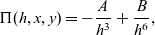 \begin{equation} \Pi(h,x,y) = -\frac{A}{h^3} +\frac{B}{h^6},\end{equation}
suggested, for example, by Pismen [Reference Pismen29]. Here A and B are positive parameters that measure the relative contributions of the long-range forces (the $1/h^3$
term) and the short-range ones (the
$1/h^3$
term) and the short-range ones (the $1/h^6$
term). However, we will see that both of these constants can be scaled out of the mathematical problem. Equation (2.3) uses the exponent
$1/h^6$
term). However, we will see that both of these constants can be scaled out of the mathematical problem. Equation (2.3) uses the exponent $-3$
for the long-range forces and
$-3$
for the long-range forces and $-6$
for the short-range forces as in Honisch et al. [Reference Honisch, Lin, Heuer, Thiele and Gurevich17]. Other choices include the pairs of long- and short-range exponents
$-6$
for the short-range forces as in Honisch et al. [Reference Honisch, Lin, Heuer, Thiele and Gurevich17]. Other choices include the pairs of long- and short-range exponents $(-2,-3)$
,
$(-2,-3)$
, $(-3,-4)$
and
$(-3,-4)$
and $(-3,-9)$
discussed by [Reference Bertozzi, Grün and Witelski4,Reference Schwartz and Eley33,Reference Sibley, Nold, Savva and Kalliadasis36]. In terms of the classification of Bertozzi et al. [4, Definition 1], the choice
$(-3,-9)$
discussed by [Reference Bertozzi, Grün and Witelski4,Reference Schwartz and Eley33,Reference Sibley, Nold, Savva and Kalliadasis36]. In terms of the classification of Bertozzi et al. [4, Definition 1], the choice $(-3,-6)$
is admissible (as are all the other pairs above), and falls in their region II; we expect that choosing other admissible exponent pairs will give qualitatively the same results as those obtained here.
$(-3,-6)$
is admissible (as are all the other pairs above), and falls in their region II; we expect that choosing other admissible exponent pairs will give qualitatively the same results as those obtained here.
In what follows, we study thin films on both homogeneous and non-homogeneous substrates. In the non-homogeneous case, we will modify (2.3) by assuming that the Derjaguin pressure term $\Pi$
changes periodically in the x-direction with period L. The appropriate forms of
$\Pi$
changes periodically in the x-direction with period L. The appropriate forms of $\Pi$
in the non-homogeneous case are discussed in Section 5.
$\Pi$
in the non-homogeneous case are discussed in Section 5.
Hence, in order better to understand solutions of (2.1), we study its one-dimensional version,
 \begin{equation} h_t = (Q(h)P(h,x)_x)_x, \; \; 0< x<L.\end{equation}
We start by characterising steady-state solutions of (2.4) subject to periodic boundary conditions at $x=0$
and
$x=0$
and $x=L$
. In other words, we seek steady-state solutions h(x) of (2.4) satisfying the non-local boundary value problem
$x=L$
. In other words, we seek steady-state solutions h(x) of (2.4) satisfying the non-local boundary value problem
 \begin{equation} \gamma h_{xx} + \frac{B}{h^6} - \frac{A}{h^3} -\frac{1}{L} \int_0^L\left[ \frac{B}{h^6} - \frac{A}{h^3}\right] \, \hbox{d}{x} = 0,\; \; 0< x <L,\end{equation}
subject to the constraint
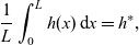 \begin{equation} \frac{1}{L}\int_0^L h(x) \, \hbox{d}{x} = h^*,\end{equation}
where the constant $h^*\,(>0)$
denotes the (scaled) average film thickness, and the periodic boundary conditions
$h^*\,(>0)$
denotes the (scaled) average film thickness, and the periodic boundary conditions
 \begin{equation} h(0)=h(L), \quad h_x(0)=h_x(L).\end{equation}
Now we non-dimensionalise. Setting
 \begin{equation} H = \left( \frac{B}{A} \right)^{1/3}, \; \; h= H \tilde{h} \quad \hbox{and} \quad x = L\tilde{x},\end{equation}
in (2.5) and removing the tildes, we obtain
 \begin{equation}\epsilon^2 h_{xx} + f(h) - \int_0^1 f(h) \, \hbox{d}{x} = 0,\; \; 0< x <1,\end{equation}
where
 \begin{equation}f(h)= \frac{1}{h^6}-\frac{1}{h^3},\end{equation}
and
 \begin{equation} \epsilon^2 = \frac{\gamma B^{4/3}}{L^2 A^{7/3}},\end{equation}
subject to the periodic boundary conditions
 \begin{equation}h(0)=h(1), \quad h_x(0)=h_x(1),\end{equation}
and the volume constraint
 \begin{equation} \int_0^1 h(x) \, \hbox{d}{x} = \bar{h},\end{equation}
where
 \begin{equation}\bar{h}= \frac{h^*A^{1/3}}{B^{1/3}}.\end{equation}
Note that the problem (2.9)–(2.14) is very similar to the corresponding steady-state problem for the Cahn–Hilliard equation considered as a bifurcation problem in the parameters $\bar{h}$
and
$\bar{h}$
and $\epsilon$
by Eilbeck et al. [Reference Eilbeck, Furter and Grinfeld12]. The boundary conditions considered in that work were the physically natural double Neumann conditions. The periodic boundary conditions (2.12) in the present problem slightly change the analysis, but our general approach in characterising different bifurcation regimes still follows that of Eilbeck et al. [Reference Eilbeck, Furter and Grinfeld12], though the correct interpretation of the limit as
$\epsilon$
by Eilbeck et al. [Reference Eilbeck, Furter and Grinfeld12]. The boundary conditions considered in that work were the physically natural double Neumann conditions. The periodic boundary conditions (2.12) in the present problem slightly change the analysis, but our general approach in characterising different bifurcation regimes still follows that of Eilbeck et al. [Reference Eilbeck, Furter and Grinfeld12], though the correct interpretation of the limit as $\epsilon \to 0^+$
is that now we let the surface tension
$\epsilon \to 0^+$
is that now we let the surface tension $\gamma$
go to zero. In particular, we perform a Liapunov–Schmidt reduction to determine the local behaviour close to bifurcation points and then use AUTO (in the present work, we use the AUTO-07p version [Reference Doedel and Oldeman11]) to explore the global structure of branches of steady-state solutions both for the spatially homogeneous case and for the spatially non-homogeneous case in the case of an x-periodically patterned substrate.
$\gamma$
go to zero. In particular, we perform a Liapunov–Schmidt reduction to determine the local behaviour close to bifurcation points and then use AUTO (in the present work, we use the AUTO-07p version [Reference Doedel and Oldeman11]) to explore the global structure of branches of steady-state solutions both for the spatially homogeneous case and for the spatially non-homogeneous case in the case of an x-periodically patterned substrate.
We first investigate the homogeneous case, and having elucidated the structure of the bifurcations of non-trivial solutions from the constant solution $h=\bar{h}$
in that case in Sections 3 and 4, we study forced rotational (O(2)) symmetry breaking in the non-homogeneous case in Section 5. In Appendix A, we present a general result about O(2) symmetry breaking in the spatially non-homogeneous case. It shows that in the spatially non-homogeneous case, only two steady-state solutions remain from the orbit of solutions of (2.9)–(2.14) induced by its O(2) invariance. We concentrate on the simplest steady-state solutions of (2.9)–(2.14), as by a result of Laugesen and Pugh [25, Theorem 1] only such solutions, that is, constant solutions and those having only one extremum point, are linearly stable in the homogeneous case. For information about dynamics of one-dimensional thin-film equations the reader should also consult Zhang [Reference Zhang46].
$h=\bar{h}$
in that case in Sections 3 and 4, we study forced rotational (O(2)) symmetry breaking in the non-homogeneous case in Section 5. In Appendix A, we present a general result about O(2) symmetry breaking in the spatially non-homogeneous case. It shows that in the spatially non-homogeneous case, only two steady-state solutions remain from the orbit of solutions of (2.9)–(2.14) induced by its O(2) invariance. We concentrate on the simplest steady-state solutions of (2.9)–(2.14), as by a result of Laugesen and Pugh [25, Theorem 1] only such solutions, that is, constant solutions and those having only one extremum point, are linearly stable in the homogeneous case. For information about dynamics of one-dimensional thin-film equations the reader should also consult Zhang [Reference Zhang46].
In what follows, we use $\|\cdot\|_2$
to denote
$\|\cdot\|_2$
to denote $L^2([0,1])$
norms.
$L^2([0,1])$
norms.
3 Liapunov–Schmidt reduction in the spatially homogeneous case
We start by performing an analysis of the dependence of the global structure of branches of steady-state solutions of the problem in the spatially homogeneous case given by (2.9)–(2.14) on the parameters $\bar{h}$
and
$\bar{h}$
and $\epsilon$
.
$\epsilon$
.
In what follows, we do not indicate explicitly the dependence of the operators on the parameters $\bar{h}$
and
$\bar{h}$
and $\epsilon$
, and all of the calculations are performed for a fixed value of
$\epsilon$
, and all of the calculations are performed for a fixed value of $\bar{h}$
and close to a bifurcation point
$\bar{h}$
and close to a bifurcation point $\epsilon=\epsilon_k$
for
$\epsilon=\epsilon_k$
for $k=1,2,3,\ldots$
defined below.
$k=1,2,3,\ldots$
defined below.
We set $v=h-\bar{h}$
, so that
$v=h-\bar{h}$
, so that $v=v(x)$
has zero mean, and rewrite (2.9) as
$v=v(x)$
has zero mean, and rewrite (2.9) as
 \begin{equation}G(v) = 0,\end{equation}
where
 \begin{equation}G(v)=\epsilon^2 v_{xx} + f(v+\bar{h}) - \int_{0}^{1}f(v(x)+\bar{h}) \, \hbox{d}{x}.\end{equation}
If we set
 \begin{equation}H = \left\{w\in C(0,1) \,:\, \int_{0}^{1} w(x) \, \hbox{d}{x} =0\right\},\end{equation}
where G is an operator from $D(G)\subset H \rightarrow H$
, then D(G) is given by
$D(G)\subset H \rightarrow H$
, then D(G) is given by
 \begin{equation}D(G) = \left\{v\in C^2(0,1) \,:\, v(0)=v(1), \, v_{x}(0)=v_{x}(1), \, \int_{0}^{1} v(x) \, \hbox{d}{x} =0 \right\}.\end{equation}
The linearisation of G at v applied to w is defined by
 \begin{equation}dG(v) w = \lim_{\tau\to0} \frac{G(v+\tau w)-G(v)}{\tau}.\end{equation}
We denote dG(0) by S, so that S applied to w is given by
 \begin{equation}S w = \epsilon^2 w_{xx} + f'(\bar{h})w.\end{equation}
To locate the bifurcation points, we have to find the non-trivial solutions of the equation $S w = 0$
subject to
$S w = 0$
subject to
 \begin{equation}w(0)=w(1), \quad \quad w_x(0)=w_x(1).\end{equation}
The kernel of S is non-empty and two-dimensional when
 \begin{equation}\epsilon = \epsilon_{k} = \frac{\sqrt{f'(\bar{h})}}{2k\pi}\quad \textrm{for} \quad k = 1,2,3,\ldots,\end{equation}
and is spanned by $\cos(2k\pi x)$
and
$\cos(2k\pi x)$
and $\sin(2k\pi x)$
. That these values of
$\sin(2k\pi x)$
. That these values of $\epsilon$
correspond to bifurcation points follows from two theorems of Vanderbauwhede [40, Theorems 2 and 3].
$\epsilon$
correspond to bifurcation points follows from two theorems of Vanderbauwhede [40, Theorems 2 and 3].
In a neighbourhood of a bifurcation point $(\epsilon_k,0)$
in
$(\epsilon_k,0)$
in $(\epsilon,v)$
space, solutions of
$(\epsilon,v)$
space, solutions of $G(v)=0$
on H are in one-to-one correspondence with solutions of the reduced system of equations on
$G(v)=0$
on H are in one-to-one correspondence with solutions of the reduced system of equations on $\mathbb{R}^2$
,
$\mathbb{R}^2$
,
 \begin{equation}g_1(x,y,\epsilon)=0, \quad g_2(x,y,\epsilon)=0,\end{equation}
for some functions $g_1$
and
$g_1$
and $g_2$
to be obtained through the Liapunov–Schmidt reduction [Reference Golubitsky and Schaeffer16].
$g_2$
to be obtained through the Liapunov–Schmidt reduction [Reference Golubitsky and Schaeffer16].
To set up the Liapunov–Schmidt reduction, we decompose D(G) and H as follows:
 \begin{equation}D(G)= \hbox{ker}\,S \oplus M,\end{equation}
and
 \begin{equation}H = N \oplus \hbox{range} \, S.\end{equation}
Since S is self-adjoint with respect to the $L^2$
-inner product denoted by
$L^2$
-inner product denoted by $\langle \cdot, \cdot \rangle$
, we can choose
$\langle \cdot, \cdot \rangle$
, we can choose
 \begin{equation}M = N = \hbox{span}\, \left\{ \cos(2kx), \sin(2kx) \right\},\end{equation}
and denote the above basis for M by $\left\{ w_1, w_2 \right\}$
and for N by
$\left\{ w_1, w_2 \right\}$
and for N by $\left\{ w_1^*, w_2^* \right\}$
. We also denote the projection of H onto
$\left\{ w_1^*, w_2^* \right\}$
. We also denote the projection of H onto $\hbox{range}\, S$
by E.
$\hbox{range}\, S$
by E.
Since the present problem is invariant with respect to the group O(2), the functions $g_1$
and
$g_1$
and $g_2$
must have the form
$g_2$
must have the form
 \begin{equation}g_1(x,y,\epsilon) = xp(x^2+y^2,\epsilon), \quad g_2(x,y,\epsilon) = yp(x^2+y^2,\epsilon),\end{equation}
for some function $p(\cdot,\cdot)$
[Reference Chossat and Lauterbach9], which means that in order to determine the bifurcation structure, the only terms that need to be computed are
$p(\cdot,\cdot)$
[Reference Chossat and Lauterbach9], which means that in order to determine the bifurcation structure, the only terms that need to be computed are $g_{1,x\epsilon}$
and
$g_{1,x\epsilon}$
and $g_{1,xxx}$
, as these immediately give
$g_{1,xxx}$
, as these immediately give $g_{2,y\epsilon}$
and
$g_{2,y\epsilon}$
and $g_{2,yyy}$
and all of the other second and third partial derivatives of
$g_{2,yyy}$
and all of the other second and third partial derivatives of $g_1$
and
$g_1$
and $g_2$
are identically zero.
$g_2$
are identically zero.
Following Golubitsky and Schaeffer [Reference Golubitsky and Schaeffer16], we have
 \begin{eqnarray}g_{1,x\epsilon}& = & \langle w_1^*, dG_{\epsilon}(w_1)-d^2G(w_1, S^{-1}E G_{\epsilon}(0)) \rangle, \end{eqnarray}
 \begin{eqnarray}g_{1,xxx}& = &\langle w_1^*, d^3G(w_1,w_1,w_1) - 3d^2G(w_1,S^{-1}E[d^2G(w_1,w_1)]) \rangle, \end{eqnarray}
where
 \begin{equation} d^rG(z_1,\ldots,z_r)=\left. \frac{\partial^r}{\partial t_1\ldots\partial t_r}G (t_1z_1+\ldots+t_rz_r) \right\vert_{t_1=\ldots=t_r=0} \quad \textrm{for} \quad r = 1, 2, 3, \ldots,\end{equation}
and we choose
 \begin{equation}w_1= w_1^*=\cos(2k\pi x),\end{equation}
where $w_1 \in \hbox{ker}\ S$
and
$w_1 \in \hbox{ker}\ S$
and $w_1^* \in (\hbox{range}\ S)^{\perp}$
. In particular, from (3.16) we have
$w_1^* \in (\hbox{range}\ S)^{\perp}$
. In particular, from (3.16) we have
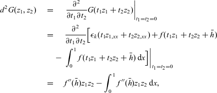 \begin{eqnarray}d^2G(z_1,z_2)& = & \left. \frac{\partial^2}{\partial t_1\partial t_2} G(t_1z_1+t_2z_2) \right\vert_{t_1=t_2=0} \nonumber\\& = & \frac{\partial^2}{\partial t_1\partial t_2} \Big[ \epsilon_k (t_1z_{1,xx}+t_2z_{2,xx}) + f(t_1z_1+t_2z_2+\bar{h})\nonumber \\& \qquad - & \left. \int_{0}^{1} f(t_1z_1+t_2z_2+\bar{h}) \, \hbox{d}{x} \Big]\right\vert_{t_1=t_2=0}\nonumber \\ & = & f''(\bar{h})z_1z_2 - \int_{0}^{1} f''(\bar{h})z_1z_2 \, \hbox{d}{x},\end{eqnarray}
and so
 \begin{eqnarray}d^2G(\cos(2k\pi x),\cos(2k\pi x))& = & f''(\bar{h})\cos^2(2k\pi x)- \int_{0}^{1} f''(\bar{h})\cos^2(2k\pi x) \, \hbox{d}{x} \nonumber\\& = & f''(\bar{h})\cos^2(2k\pi x)- \frac{1}{2} f''(\bar{h}).\end{eqnarray}
To obtain $S^{-1}E [d^2G(w_1,w_1)]$
, which we denote by R(x), so that
$S^{-1}E [d^2G(w_1,w_1)]$
, which we denote by R(x), so that $SR=E[d^2G(w_1,w_1)]$
, we use the definition of
$SR=E[d^2G(w_1,w_1)]$
, we use the definition of $\epsilon_k$
given in (3.8) and solve the second-order ordinary differential equation satisfied by R(x),
$\epsilon_k$
given in (3.8) and solve the second-order ordinary differential equation satisfied by R(x),
 \begin{equation}R_{xx} + 4k^2\pi^2 R = 4k^2\pi^2 \frac{f''(\bar{h})}{f'(\bar{h})}\cos^2(2k\pi x) - 2k^2\pi^2 \frac{f''(\bar{h})}{f'(\bar{h})},\end{equation}
subject to
 \begin{equation}R(0)=R(1)\quad \textrm{and} \quad R_x(0)=R_x(1),\end{equation}
in $\hbox{ker}\, S$
. We obtain
$\hbox{ker}\, S$
. We obtain
 \begin{equation}R(x) = S^{-1}E[d^2G(w_1,w_1)] = -\frac{1}{6}\frac{f''(\bar{h})}{f'(\bar{h})} \cos(4k\pi x),\end{equation}
and hence
 \begin{eqnarray}d^2G(w_1,S^{-1}E[d^2G(w_1,w_1)]) &=& d^2G\left(\cos(2k\pi x),-\frac{1}{6}\frac{f''(\bar{h})}{f'(\bar{h})} \cos(4k\pi x)\right) \nonumber\\& = & f''(\bar{h})\cos(2k\pi x)\left(-\frac{1}{6}\frac{f''(\bar{h})}{f'(\bar{h})} \cos(4k\pi x)\right) \nonumber\\& & - \int_{0}^{1} f''(\bar{h})\cos(2k\pi x)\left(-\frac{1}{6}\frac{f''(\bar{h})}{f'(\bar{h})} \cos(4k\pi x)\right) \hbox{d}{x} \nonumber\\& = & - \frac{1}{6}\frac{[f''(\bar{h})]^2}{f'(\bar{h})} \cos(2k\pi x)\cos(4k\pi x).\end{eqnarray}
In addition, from (3.16) we have
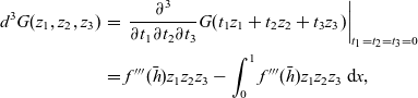 \begin{eqnarray}d^3G(z_1,z_2,z_3)& = & \left. \frac{\partial^3}{\partial t_1\partial t_2\partial t_3}G(t_1z_1+t_2z_2+t_3z_3)\right\vert_{t_1=t_2=t_3=0} \nonumber\\& = & f'''(\bar{h})z_1z_2z_3 - \int_0^1 f'''(\bar{h})z_1z_2z_3 \, \hbox{d}{x},\end{eqnarray}
and therefore
 \begin{eqnarray}d^3G(\cos(2k\pi x),\cos(2k\pi x),\cos(2k\pi x))& = & f'''(\bar{h})\cos^3(2k\pi x) - \int_{0}^{1} f'''(\bar{h})\cos^3(2k\pi x) \, \hbox{d}{x} \nonumber\\& = & f'''(\bar{h})\cos^3(2k\pi x).\end{eqnarray}
Putting all of the information in (3.23) and (3.25) into (3.15) we obtain
 \begin{eqnarray}g_{1,xxx}& = & \langle w_1^*, d^3G(w_1,w_1,w_1) - 3d^2G(w_1,S^{-1}E[d^2G(w_1,w_1)]) \rangle \nonumber\\& = & \int_{0}^{1} \cos(2k\pi x)\left[f'''(\bar{h})\cos^3(2k\pi x)-3\left(-\frac{1}{6}\frac{[f''(\bar{h})]^2}{f'(\bar{h})} \cos(2k\pi x)\cos(4k\pi x)\right)\right]\, \hbox{d}{x} \nonumber\\& = & \frac{3}{8}f'''(\bar{h}) + \frac{1}{8}\frac{[f''(\bar{h})]^2}{f'(\bar{h})}.\end{eqnarray}
In addition, $G_{\epsilon}(v)= v_{xx}$
, so that
$G_{\epsilon}(v)= v_{xx}$
, so that $G_{\epsilon}(0)= 0$
at
$G_{\epsilon}(0)= 0$
at $v=0$
, and hence we have
$v=0$
, and hence we have
 \begin{equation}d^2G(w_k,S^{-1}EG_{\epsilon}(0))= 0.\end{equation}
Furthermore, since $dG_{\epsilon}(w)= w_{xx}$
, from (3.14) we obtain
$dG_{\epsilon}(w)= w_{xx}$
, from (3.14) we obtain
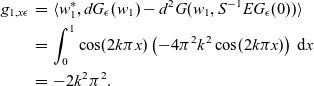 \begin{eqnarray}g_{1,x\epsilon}& = & \langle w_1^*, dG_{\epsilon}(w_1)-d^2G(w_1, S^{-1}EG_{\epsilon}(0)) \rangle \nonumber\\& = & \int_{0}^{1} \cos(2k\pi x) \left(-4\pi ^2 k^2 \cos(2k\pi x)\right)\, \hbox{d}{x} \nonumber\\& = & -2 k^2 \pi^2.\end{eqnarray}
Referring to (3.13) and the argument following that equation, the above analysis shows that as long as $f'(\bar{h})>0$
at
$f'(\bar{h})>0$
at $\epsilon=\epsilon_k$
a circle of equilibria bifurcates from the constant solution
$\epsilon=\epsilon_k$
a circle of equilibria bifurcates from the constant solution $h \equiv \bar{h}$
. The direction of bifurcation is locally determined by the sign of
$h \equiv \bar{h}$
. The direction of bifurcation is locally determined by the sign of $g_{1,xxx}$
given by (3.26). Hence, using
$g_{1,xxx}$
given by (3.26). Hence, using $1/\epsilon$
as the bifurcation parameter, the bifurcation of non-trivial equilibria is supercritical if
$1/\epsilon$
as the bifurcation parameter, the bifurcation of non-trivial equilibria is supercritical if $g_{1,xxx}$
is negative and subcritical if it is positive.
$g_{1,xxx}$
is negative and subcritical if it is positive.
By finding the values of $\bar{h}$
where
$\bar{h}$
where $g_{1,xxx}$
given by (3.26) with f(h) given by (2.10) is zero, we finally obtain the following proposition:
$g_{1,xxx}$
given by (3.26) with f(h) given by (2.10) is zero, we finally obtain the following proposition:
Proposition 1 Bifurcations of non-trivial solutions from the constant solution $h=\bar{h}$
of the problem (2.9)–(2.14) are supercritical if
$h=\bar{h}$
of the problem (2.9)–(2.14) are supercritical if $1.289 < \bar{h} < 1.747$
and subcritical if
$1.289 < \bar{h} < 1.747$
and subcritical if $1.259 < \bar{h} <1.289$
or if
$1.259 < \bar{h} <1.289$
or if $\bar{h} > 1.747$
.
$\bar{h} > 1.747$
.
Proof. The constant solution $h \equiv \bar{h}$
will lose stability as
$h \equiv \bar{h}$
will lose stability as $\epsilon$
is decreased only if
$\epsilon$
is decreased only if $f'(\bar{h}) >0$
. i.e. if
$f'(\bar{h}) >0$
. i.e. if $-6/{\bar{h}}^7 + 3/{\bar{h}}^4 > 0$
, for
$-6/{\bar{h}}^7 + 3/{\bar{h}}^4 > 0$
, for $\bar{h} > 2^{1/3} \approx1.259$
. From (3.26) we have that
$\bar{h} > 2^{1/3} \approx1.259$
. From (3.26) we have that
 \begin{equation}g_{1,xxx} = \frac{57 \bar{h}^6-426 \bar{h}^3+651}{2\bar{h}^9(\bar{h}^3-2)},\end{equation}
so that $g_{1,xxx}<0$
if
$g_{1,xxx}<0$
if $\bar{h} \in (1.289, 1.747)$
giving the result.
$\bar{h} \in (1.289, 1.747)$
giving the result.
For $\bar{h} \leqslant 2^{1/3}$
there are no bifurcations from the constant solution
$\bar{h} \leqslant 2^{1/3}$
there are no bifurcations from the constant solution $h = \bar{h}$
. Furthermore, we have the following proposition:
$h = \bar{h}$
. Furthermore, we have the following proposition:

Proof. Assume that such a non-trivial solution exists. Then, since $\bar{h} \leq 1$
, its global minimum, achieved at some point
$\bar{h} \leq 1$
, its global minimum, achieved at some point $x_0\in (0,1)$
, must be less than 1. (We may take the point
$x_0\in (0,1)$
, must be less than 1. (We may take the point $x_0$
to be an interior point by translation invariance.) But then
$x_0$
to be an interior point by translation invariance.) But then
 \begin{equation}\epsilon^2 h_{xx}(x_0) = \int_0^1 f(h)\, \hbox{d}{x} - f(h(x_0)) < 0,\end{equation}
so the point $x_0$
cannot be a minimum.
$x_0$
cannot be a minimum.
4 Two-parameter continuation of solutions in the spatially homogeneous case
To describe the change in the global structure of branches of steady-state solutions of the problem (2.9)–(2.14) as $\bar{h}$
and
$\bar{h}$
and $\epsilon$
are varied, we use AUTO [Reference Doedel and Oldeman11] and our results are summarised in Figure 1.
$\epsilon$
are varied, we use AUTO [Reference Doedel and Oldeman11] and our results are summarised in Figure 1.
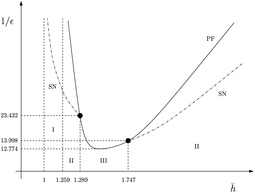
The global structure of branches of steady-state solutions with a unique maximum, including both saddle-node (SN) (shown with dash-dotted curves) and pitchfork (PF) bifurcation branches (shown with solid curves). The nucleation regime $1 < \bar{h} < 2^{1/3} \approx 1.259$
(Regime I), the metastable regime
$1 < \bar{h} < 2^{1/3} \approx 1.259$
(Regime I), the metastable regime $2^{1/3} < \bar{h} < 1.289$
and
$2^{1/3} < \bar{h} < 1.289$
and $\bar{h} > 1.747$
(Regime II), and the unstable regime
$\bar{h} > 1.747$
(Regime II), and the unstable regime $1.289 < \bar{h} < 1.747$
(Regime III) are also indicated.
$1.289 < \bar{h} < 1.747$
(Regime III) are also indicated.
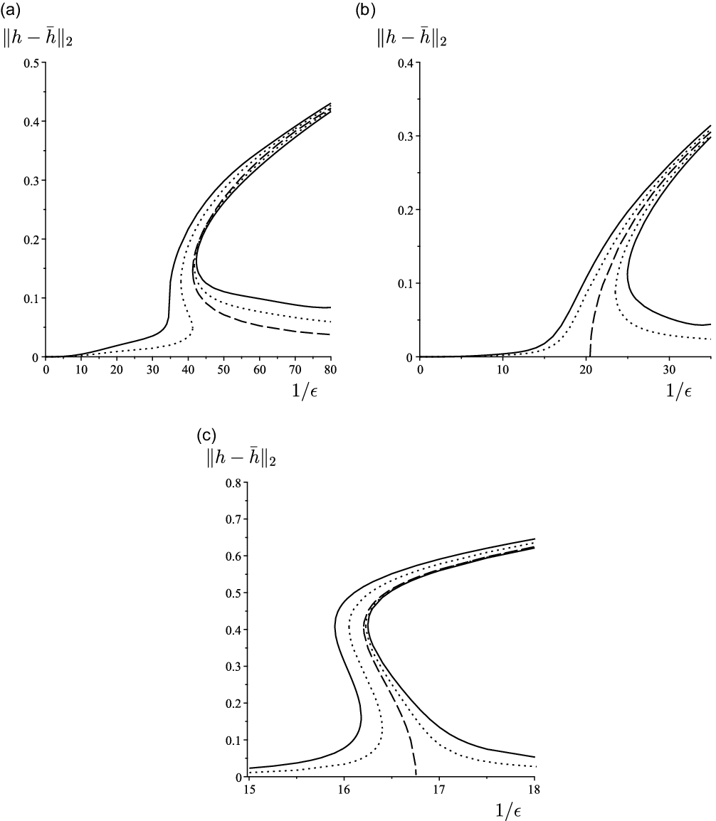
Bifurcation diagrams of solutions with a unique maximum, showing $\|h-\bar{h} \|_2$
plotted as a function of
$\|h-\bar{h} \|_2$
plotted as a function of $1/\epsilon$
when the disjoining pressure is
$1/\epsilon$
when the disjoining pressure is $\Pi_{\rm LR}$
for
$\Pi_{\rm LR}$
for $\rho=0$
(dashed curves),
$\rho=0$
(dashed curves), $\rho=0.005$
(dotted curves) and
$\rho=0.005$
(dotted curves) and $\rho=0.05$
(solid curves) for (a)
$\rho=0.05$
(solid curves) for (a) $\bar{h}=1.24$
, (b)
$\bar{h}=1.24$
, (b) $\bar{h}=1.3$
and (c)
$\bar{h}=1.3$
and (c) $\bar{h}=2$
, corresponding to Regimes I, III and II, respectively.
$\bar{h}=2$
, corresponding to Regimes I, III and II, respectively.
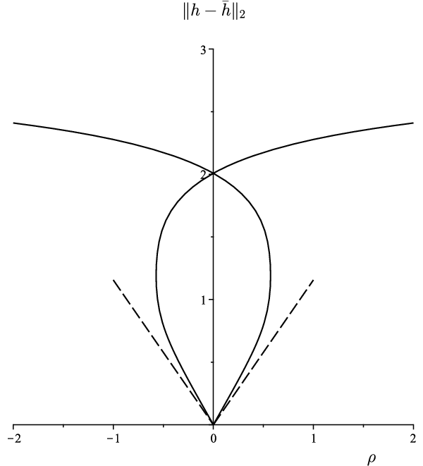
Bifurcation diagram for steady-state solutions with a unique maximum showing $\|h-\bar{h}\|_2$
plotted as a function of
$\|h-\bar{h}\|_2$
plotted as a function of $\rho$
when the disjoining pressure is
$\rho$
when the disjoining pressure is $\Pi_{\rm LR}$
, for
$\Pi_{\rm LR}$
, for $\bar{h}=3$
and
$\bar{h}=3$
and $1/\epsilon=50$
. The leading-order dependence of
$1/\epsilon=50$
. The leading-order dependence of $\|h-\bar{h}\|_2$
on
$\|h-\bar{h}\|_2$
on $\rho$
as
$\rho$
as $\rho \to 0$
, given by (5.8), is shown with dashed lines.
$\rho \to 0$
, given by (5.8), is shown with dashed lines.
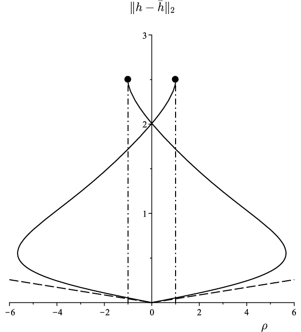
Bifurcation diagram showing $\|h-\bar{h}\|_2$
plotted as a function of
$\|h-\bar{h}\|_2$
plotted as a function of $\rho$
when the disjoining pressure is
$\rho$
when the disjoining pressure is $\Pi_{\rm SR}$
, for
$\Pi_{\rm SR}$
, for $\bar{h}=3$
and
$\bar{h}=3$
and $1/\epsilon=50$
. The leading-order dependence of
$1/\epsilon=50$
. The leading-order dependence of $\|h-\bar{h}\|_2$
on
$\|h-\bar{h}\|_2$
on $\rho$
as
$\rho$
as $\rho \to 0$
, given by (5.9), is shown with dashed lines. Note that the upper branches of solutions cannot be extended beyond
$\rho \to 0$
, given by (5.9), is shown with dashed lines. Note that the upper branches of solutions cannot be extended beyond $|\rho|=1$
(indicated by filled circles).
$|\rho|=1$
(indicated by filled circles).
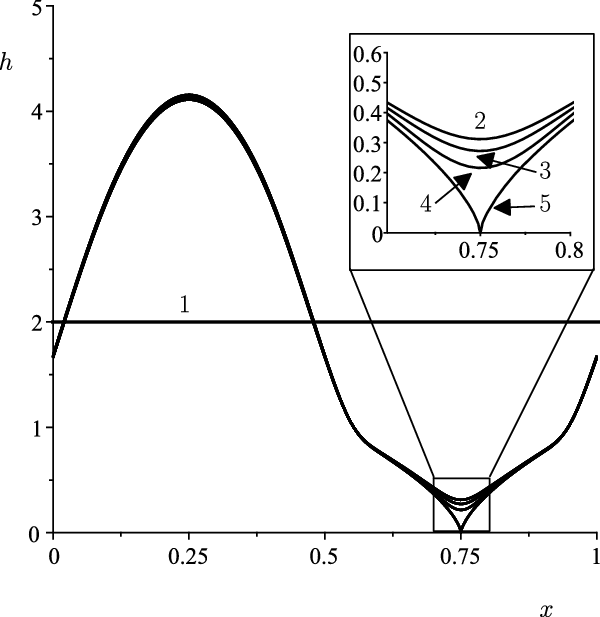
Solutions h(x) when the disjoining pressure is $\Pi_{\rm SR}$
for
$\Pi_{\rm SR}$
for $\bar{h}=2$
and
$\bar{h}=2$
and $1/\epsilon=30$
for
$1/\epsilon=30$
for $\rho=0$
, 0.97, 0.98, 0.99 and 1, denoted by ‘1’, ‘2’, ‘3’, ‘4’ and ‘5’, respectively, showing convergence of strictly positive solutions to a non-strictly positive one as
$\rho=0$
, 0.97, 0.98, 0.99 and 1, denoted by ‘1’, ‘2’, ‘3’, ‘4’ and ‘5’, respectively, showing convergence of strictly positive solutions to a non-strictly positive one as $\rho \to 1^-$
.
$\rho \to 1^-$
.
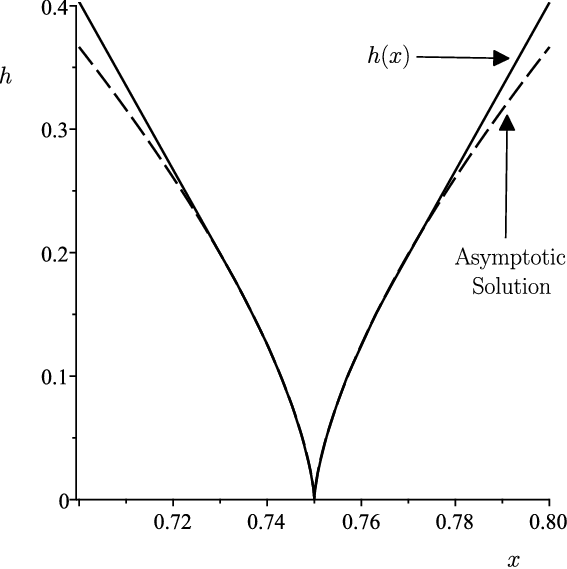
Detail near $x=3/4$
of the solution h(x) shown with solid line when the disjoining pressure is
$x=3/4$
of the solution h(x) shown with solid line when the disjoining pressure is $\Pi_{\rm SR}$
and
$\Pi_{\rm SR}$
and $\rho=1$
, and the two-term asymptotic solution given by (5.10) shown with dashed lines for
$\rho=1$
, and the two-term asymptotic solution given by (5.10) shown with dashed lines for $\bar{h}=2$
and
$\bar{h}=2$
and $\epsilon=1/30$
.
$\epsilon=1/30$
.
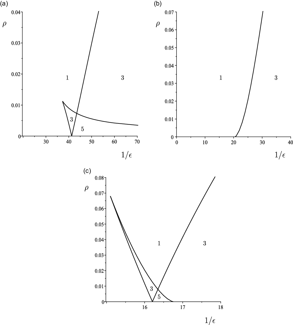
Multiplicity of strictly positive solutions with a unique maximum in the $(1/\epsilon,\rho)$
-plane when the disjoining pressure is
$(1/\epsilon,\rho)$
-plane when the disjoining pressure is $\Pi_{\rm LR}$
for (a)
$\Pi_{\rm LR}$
for (a) $\bar{h}=1.24$
(Regime I), (b)
$\bar{h}=1.24$
(Regime I), (b) $\bar{h}=1.3$
(Regime III) and (c)
$\bar{h}=1.3$
(Regime III) and (c) $\bar{h}=2$
(Regime II).
$\bar{h}=2$
(Regime II).
Multiplicity of strictly positive solutions with a unique maximum in the $(1 / \epsilon, \rho)$
-plane when the disjoining pressure is
$(1 / \epsilon, \rho)$
-plane when the disjoining pressure is $\Pi_{\rm SR}$
for (a)
$\Pi_{\rm SR}$
for (a) $\bar{h}=1.24$
(Regime I), (b)
$\bar{h}=1.24$
(Regime I), (b) $\bar{h}=1.3$
(Regime III) and (c)
$\bar{h}=1.3$
(Regime III) and (c) $\bar{h}=2$
(Regime II).
$\bar{h}=2$
(Regime II).

Bifurcation diagram of steady-state solutions with $\bar{h} = 2$
(Regime II) for
$\bar{h} = 2$
(Regime II) for $\rho=0$
(dashed curves) and
$\rho=0$
(dashed curves) and $\rho=0.005$
(solid curves) indicating the different branches of steady-state solutions.
$\rho=0.005$
(solid curves) indicating the different branches of steady-state solutions.
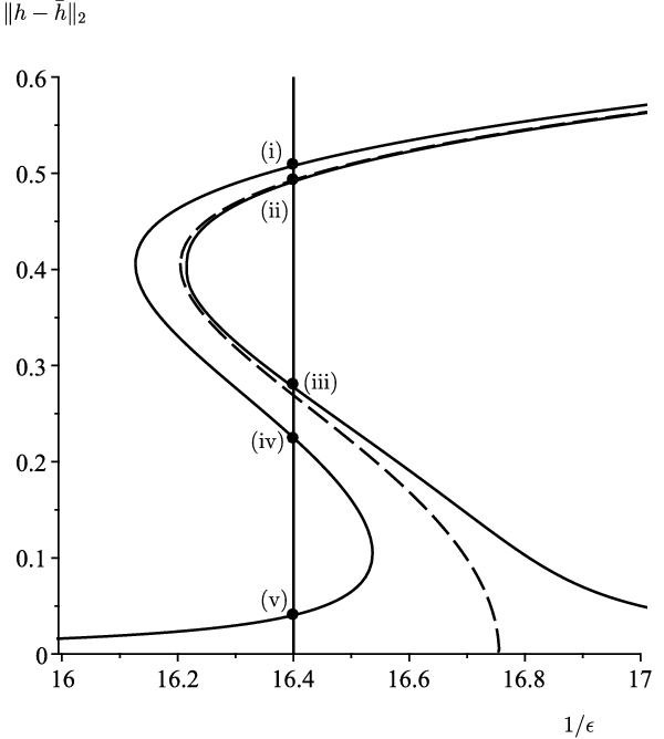
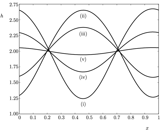
Steady-state solutions on the five branches of solutions indicated in Figure 9 by (i)–(v).
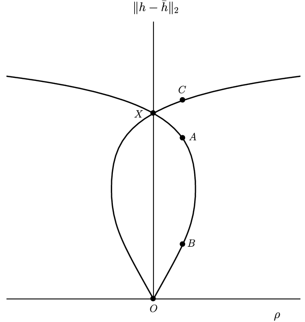
A sketch of the bifurcation diagram plotted in Figure 3 with the different solution branches labelled.
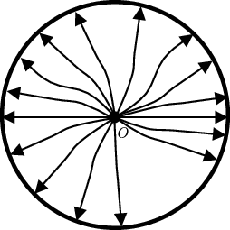
Sketch of the global attractor for $\rho=0$
. The circle represents the O(2) orbit of steady-state solutions and O represents the constant solution
$\rho=0$
. The circle represents the O(2) orbit of steady-state solutions and O represents the constant solution $h(x)=\bar{h}$
.
$h(x)=\bar{h}$
.
Sketch of the global attractor for small non-zero values of $|\rho|$
. The points A, B, C correspond to the steady-state solutions labelled in Figure 11.
$|\rho|$
. The points A, B, C correspond to the steady-state solutions labelled in Figure 11.

Figure 1 shows a curve of saddle-node (SN) bifurcations which originates from $\bar{h} \approx 1.289$
at
$\bar{h} \approx 1.289$
at $1/\epsilon \approx 23.432$
satisfies
$1/\epsilon \approx 23.432$
satisfies $\bar{h} \rightarrow1^+$
as
$\bar{h} \rightarrow1^+$
as $1/\epsilon \rightarrow \infty$
, while a curve of SN bifurcations which originates from
$1/\epsilon \rightarrow \infty$
, while a curve of SN bifurcations which originates from $\bar{h} \approx 1.747$
,
$\bar{h} \approx 1.747$
, $1/\epsilon\approx 13.998$
satisfies
$1/\epsilon\approx 13.998$
satisfies $\bar{h} \rightarrow \infty$
as
$\bar{h} \rightarrow \infty$
as $1/\epsilon \rightarrow \infty$
.
$1/\epsilon \rightarrow \infty$
.
Figure 1 identifies three different bifurcation regimes, denoted by I, II and III, with differing bifurcation behaviour occurring in the different regimes, namely (using the terminology of [Reference Eilbeck, Furter and Grinfeld12] in the context of the Cahn–Hilliard equation):
-
a ‘nucleation’ regime for $1 < \bar{h} < 2^{1/3} \approx 1.259$
(Regime I),
$1 < \bar{h} < 2^{1/3} \approx 1.259$
(Regime I), -
a ‘metastable’ regime for
$2^{1/3} < \bar{h} < 1.289$
and
$\bar{h} >1.747$
(Regime II), and -
an ‘unstable’ regime for
$1.289 < \bar{h} < 1.747$
(Regime III).




In Regime I, the constant solution $h(x)\equiv\bar{h}$
is linearly stable which follows from analysing the spectrum of the operator S for
$h(x)\equiv\bar{h}$
is linearly stable which follows from analysing the spectrum of the operator S for $f'(\bar{h})<0$
in (3.6) and (3.7), but under sufficiently large perturbations, the system will evolve to a non-constant steady-state solution. See [Reference Laugesen and Pugh25] for an extensive discussion of the stability analysis of steady-state solutions to thin-film equations.
$f'(\bar{h})<0$
in (3.6) and (3.7), but under sufficiently large perturbations, the system will evolve to a non-constant steady-state solution. See [Reference Laugesen and Pugh25] for an extensive discussion of the stability analysis of steady-state solutions to thin-film equations.
In Regime II, as $\epsilon$
is decreased the constant solution
$\epsilon$
is decreased the constant solution $h(x)\equiv \bar{h}$
loses stability through a subcritical bifurcation.
$h(x)\equiv \bar{h}$
loses stability through a subcritical bifurcation.
In Regime III, as $\epsilon$
is decreased, the constant solution
$\epsilon$
is decreased, the constant solution $h(x) \equiv \bar{h}$
loses stability through a supercritical bifurcation.
$h(x) \equiv \bar{h}$
loses stability through a supercritical bifurcation.
5 The spatially non-homogeneous case
Honisch et al. [Reference Honisch, Lin, Heuer, Thiele and Gurevich17] chose the Derjaguin disjoining pressure $\Pi(h,x,y)$
to be of the form
$\Pi(h,x,y)$
to be of the form
 \begin{equation}\Pi(h,x,y) = \left( \frac{1}{h^6}-\frac{1}{h^3} \right) (1 + \rho\, G(x,y)),\end{equation}
where the function G(x, y) models the non-homogeneity of the substrate and the parameter $\rho$
, which can be either positive or negative, is called the ‘wettability contrast’. Following Honisch et al. [Reference Honisch, Lin, Heuer, Thiele and Gurevich17], in the remainder of the present work we consider the specific case
$\rho$
, which can be either positive or negative, is called the ‘wettability contrast’. Following Honisch et al. [Reference Honisch, Lin, Heuer, Thiele and Gurevich17], in the remainder of the present work we consider the specific case
 \begin{equation}G(x,y) = \sin \left(2\pi x \right) := G(x),\end{equation}
corresponding to an x-periodically patterned (i.e. striped) substrate.
There are, however, some difficulties in accepting (5.1) as a physically realistic form of the disjoining pressure for a non-homogeneous substrate. The problems arise because the two terms in (5.1) represent rather different physical effects. Specifically, since the $1/h^6$
term models the short-range interaction amongst the molecules of the liquid and the
$1/h^6$
term models the short-range interaction amongst the molecules of the liquid and the $1/h^3$
term models the long-range interaction, assuming that both terms reflect the patterning in the substrate in exactly the same way through their dependence on the same function G(x,y) does not seem very plausible. Moreover, there are other studies which assume that the wettability of the substrate is incorporated in either the short-range interaction term (see, e.g. Thiele and Knobloch [Reference Thiele and Knobloch38] and Bertozzi et al. [Reference Bertozzi, Grün and Witelski4]) or the long-range interaction term (see, e.g. Ajaev et al. [Reference Ajaev, Gatapova and Kabov2] and Sharma et al. [Reference Sharma, Konnur and Kargupta35]), but not both simultaneously. Hence in what follows we will consider the two cases
$1/h^3$
term models the long-range interaction, assuming that both terms reflect the patterning in the substrate in exactly the same way through their dependence on the same function G(x,y) does not seem very plausible. Moreover, there are other studies which assume that the wettability of the substrate is incorporated in either the short-range interaction term (see, e.g. Thiele and Knobloch [Reference Thiele and Knobloch38] and Bertozzi et al. [Reference Bertozzi, Grün and Witelski4]) or the long-range interaction term (see, e.g. Ajaev et al. [Reference Ajaev, Gatapova and Kabov2] and Sharma et al. [Reference Sharma, Konnur and Kargupta35]), but not both simultaneously. Hence in what follows we will consider the two cases $\Pi(h,x) = \Pi_{\rm LR}(h,x)$
and
$\Pi(h,x) = \Pi_{\rm LR}(h,x)$
and $\Pi(h,x) = \Pi_{\rm SR}(h,x)$
, where LR stands for ‘long range’ and SR stands for ‘short range’, where
$\Pi(h,x) = \Pi_{\rm SR}(h,x)$
, where LR stands for ‘long range’ and SR stands for ‘short range’, where
 \begin{equation} \Pi_{\rm LR}(h,x) = \frac{1}{h^6}-\frac{1}{h^3}(1+\rho G(x)),\end{equation}
and
 \begin{equation}\Pi_{\rm SR}(h,x) = \frac{1}{h^6}(1+\rho G(x)) -\frac{1}{h^3},\end{equation}
in both of which G(x) is given by (5.2) and $\rho$
is the wettability contrast.
$\rho$
is the wettability contrast.
For small wettability contrast, $\vert\rho\vert \ll 1$
, we do not expect there to be significant differences between the influence of
$\vert\rho\vert \ll 1$
, we do not expect there to be significant differences between the influence of $\Pi_{\rm LR}$
or
$\Pi_{\rm LR}$
or $\Pi_{\rm SR}$
on the bifurcation diagrams, as these results depend only on the nature of the bifurcation in the homogeneous case
$\Pi_{\rm SR}$
on the bifurcation diagrams, as these results depend only on the nature of the bifurcation in the homogeneous case $\rho=0$
and on the symmetry groups under which the equations are invariant. To see this, consider the spatially non-homogeneous version of (2.9), that is, the boundary value problem
$\rho=0$
and on the symmetry groups under which the equations are invariant. To see this, consider the spatially non-homogeneous version of (2.9), that is, the boundary value problem
 \begin{equation}\epsilon^2 h_{xx} + f(h,x) - \int_0^1 f(h,x) \, \hbox{d}{x} = 0,\; \; 0<x<1,\end{equation}
where now
 \begin{equation}f(h,x)=\Pi_{\rm LR}(h,x) \quad \hbox{or} \quad f(h,x)= \Pi_{\rm SR}(h,x).\end{equation}
subject to the periodic boundary conditions and the volume constraint,
 \begin{equation}h(0)=h(1), \quad h_x(0)=h_x(1), \quad \hbox{and} \quad \int_0^1 h(x) \, \hbox{d}{x} = \bar{h}.\end{equation}
Seeking an asymptotic solution to (5.5)–(5.7) in the form $h(x) = \bar{h} + \rho h_1(x) + O(\rho^2)$
in the limit
$h(x) = \bar{h} + \rho h_1(x) + O(\rho^2)$
in the limit $\rho \to 0$
, by substituting this anzatz into (5.5) we find that in the case of
$\rho \to 0$
, by substituting this anzatz into (5.5) we find that in the case of $\Pi_{\rm LR}(h,x)$
we have
$\Pi_{\rm LR}(h,x)$
we have
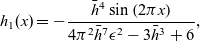 \begin{equation}h_1(x) = - \frac{\bar{h}^4\sin\left(2\pi x\right)}{4\pi^2\bar{h}^7\epsilon^2 -3\bar{h}^3 + 6},\end{equation}
while in the case of $\Pi_{\rm SR}(h,x)$
the corresponding result is
$\Pi_{\rm SR}(h,x)$
the corresponding result is
 \begin{equation} h_1(x) = \frac{\bar{h}\sin\left(2\pi x\right)}{4\pi^2\bar{h}^7\epsilon^2 - 3\bar{h}^3 + 6}.\end{equation}
For non-zero values of $\rho$
, in both the
$\rho$
, in both the $\Pi_{\rm LR}$
and
$\Pi_{\rm LR}$
and $\Pi_{\rm SR}$
cases, the changes in the bifurcation diagrams obtained in the homogeneous case (
$\Pi_{\rm SR}$
cases, the changes in the bifurcation diagrams obtained in the homogeneous case ( $\rho=0$
) are an example of forced symmetry breaking (see, e.g. Chillingworth [Reference Chillingworth8]), which we discuss further in Appendix A. More precisely, we show there that when
$\rho=0$
) are an example of forced symmetry breaking (see, e.g. Chillingworth [Reference Chillingworth8]), which we discuss further in Appendix A. More precisely, we show there that when $\rho \neq 0$
, out of the entire O(2) orbit only two equilibria are left after symmetry breaking.
$\rho \neq 0$
, out of the entire O(2) orbit only two equilibria are left after symmetry breaking.
Figure 2 shows how for small wettability contrast $\vert\rho\vert \ll 1$
, the resulting spatial non-homogeneity introduces imperfections [Reference Golubitsky and Schaeffer16] in the bifurcation diagrams of the homogeneous case
$\vert\rho\vert \ll 1$
, the resulting spatial non-homogeneity introduces imperfections [Reference Golubitsky and Schaeffer16] in the bifurcation diagrams of the homogeneous case $\rho=0$
discussed in Section 4. It presents bifurcation diagrams in Regimes I, II and III when the disjoining pressure
$\rho=0$
discussed in Section 4. It presents bifurcation diagrams in Regimes I, II and III when the disjoining pressure $\Pi_{\rm LR}$
is given by (5.3) for a range of small values of
$\Pi_{\rm LR}$
is given by (5.3) for a range of small values of $\rho$
together with the corresponding diagrams in the case
$\rho$
together with the corresponding diagrams in the case $\rho=0$
. The corresponding bifurcation diagrams when the disjoining pressure
$\rho=0$
. The corresponding bifurcation diagrams when the disjoining pressure $\Pi_{\rm SR}$
is given by (5.4) are very similar and hence are not shown here.
$\Pi_{\rm SR}$
is given by (5.4) are very similar and hence are not shown here.
For large wettability contrast, specifically for $\vert\rho\vert \geq 1$
, significant differences between the two forms of the disjoining pressure are to be expected. When using
$\vert\rho\vert \geq 1$
, significant differences between the two forms of the disjoining pressure are to be expected. When using $\Pi_{\rm LR}$
, one expects global existence of positive solutions for all values of
$\Pi_{\rm LR}$
, one expects global existence of positive solutions for all values of $\vert\rho\vert$
; see, for example, Wu and Zheng [Reference Wu and Zheng44]. On the other hand, when using
$\vert\rho\vert$
; see, for example, Wu and Zheng [Reference Wu and Zheng44]. On the other hand, when using $\Pi_{\rm SR}$
, there is the possibility of rupture of the liquid film for
$\Pi_{\rm SR}$
, there is the possibility of rupture of the liquid film for $\vert\rho\vert \geq 1$
; see, for example, [Reference Bertozzi, Grün and Witelski4,Reference Wu and Zheng44], which means in this case we do not expect positive solutions for sufficiently large values of
$\vert\rho\vert \geq 1$
; see, for example, [Reference Bertozzi, Grün and Witelski4,Reference Wu and Zheng44], which means in this case we do not expect positive solutions for sufficiently large values of $\vert\rho\vert$
.
$\vert\rho\vert$
.
In Figure 3 we plot the branches of the positive solutions of (5.5)–(5.7) with a unique maximum when the disjoining pressure is $\Pi_{\rm LR}$
for
$\Pi_{\rm LR}$
for $\bar{h}=3$
and
$\bar{h}=3$
and $1/\epsilon=50$
, so that when
$1/\epsilon=50$
, so that when $\rho=0$
we are in Regime II above the curve of pitchfork (PF) bifurcations from the constant solution shown in Figure 1. The work of Bertozzi et al. [Reference Bertozzi, Grün and Witelski4] and of Wu and Zheng [Reference Wu and Zheng44], shows that strictly positive solutions exist for all values of
$\rho=0$
we are in Regime II above the curve of pitchfork (PF) bifurcations from the constant solution shown in Figure 1. The work of Bertozzi et al. [Reference Bertozzi, Grün and Witelski4] and of Wu and Zheng [Reference Wu and Zheng44], shows that strictly positive solutions exist for all values of $|\rho|$
, i.e. beyond the range
$|\rho|$
, i.e. beyond the range $\rho \in [-2,2]$
for which we have performed the numerical calculations.
$\rho \in [-2,2]$
for which we have performed the numerical calculations.
Figure 4 shows that the situation is different when the disjoining pressure is $\Pi_{\rm SR}$
(with the same values of
$\Pi_{\rm SR}$
(with the same values of $\bar{h}$
and
$\bar{h}$
and $\epsilon$
). At
$\epsilon$
). At $\vert\rho\vert=1$
, the upper branches of solutions disappear due to rupture of the film, so that at some point
$\vert\rho\vert=1$
, the upper branches of solutions disappear due to rupture of the film, so that at some point $x_0 \in [0,1]$
we have
$x_0 \in [0,1]$
we have $h(x_0)=0$
and a strictly positive solution no longer exists, while the other two branches coalesce at a saddle-node bifurcation at
$h(x_0)=0$
and a strictly positive solution no longer exists, while the other two branches coalesce at a saddle-node bifurcation at $\vert\rho\vert \approx 5.8$
.
$\vert\rho\vert \approx 5.8$
.
Note that in Figures 3 and 4, the non-trivial ‘solution’ on the axis $\rho=0$
is, in fact, a whole O(2)-symmetric orbit of solutions predicted by the analysis leading to Figure 1.
$\rho=0$
is, in fact, a whole O(2)-symmetric orbit of solutions predicted by the analysis leading to Figure 1.
Note that when the disjoining pressure is $\Pi_{\rm SR}$
, given by (5.4), we were unable to use AUTO to continue branches of solutions beyond the rupture of the film at
$\Pi_{\rm SR}$
, given by (5.4), we were unable to use AUTO to continue branches of solutions beyond the rupture of the film at $\vert\rho\vert=1$
.
$\vert\rho\vert=1$
.
Figure 5 shows the film approaching rupture as $\rho \to 1^-$
at the point where the coefficient of the short-range term disappears when
$\rho \to 1^-$
at the point where the coefficient of the short-range term disappears when $\rho=1$
, i.e. when
$\rho=1$
, i.e. when $1 + \sin(2\pi x) = 0$
and hence at
$1 + \sin(2\pi x) = 0$
and hence at $x=3/4$
. These numerical results are consistent with the theoretical arguments of Bertozzi et al. [Reference Bertozzi, Grün and Witelski4].
$x=3/4$
. These numerical results are consistent with the theoretical arguments of Bertozzi et al. [Reference Bertozzi, Grün and Witelski4].
Investigation of the possible leading-order balance in (2.9) when the disjoining pressure is $\Pi_{\rm SR}$
and
$\Pi_{\rm SR}$
and $\rho=1$
in the limit
$\rho=1$
in the limit $x \to 3/4$
reveals that
$x \to 3/4$
reveals that $h(x) = O\left((x-3/4)^{2/3}\right)$
; continuing the analysis to higher order yields
$h(x) = O\left((x-3/4)^{2/3}\right)$
; continuing the analysis to higher order yields
 \begin{equation} h = (2\pi^2)^{\frac{1}{3}}\left(x-\frac{3}{4}\right)^{\frac{2}{3}} - \frac{4\left(4\pi^{10}\right)^{\frac13} \epsilon^2}{27} \left(x-\frac{3}{4}\right)^{\frac{4}{3}} + O\left(\left(x-\frac{3}{4}\right)^2\right).\end{equation}
Figure 6 shows the detail of the excellent agreement between the solution h(x) when $\rho=1$
and the two-term asymptotic solution given by (5.10) close to
$\rho=1$
and the two-term asymptotic solution given by (5.10) close to $x=3/4$
.
$x=3/4$
.
Figures 7 and 8 show the multiplicity of solutions with a unique maximum for the disjoining pressures $\Pi_{\rm LR}$
and
$\Pi_{\rm LR}$
and $\Pi_{\rm SR}$
, respectively, in the
$\Pi_{\rm SR}$
, respectively, in the $(1/\epsilon,\rho)$
-plane in the three regimes shown in Figure 1.
$(1/\epsilon,\rho)$
-plane in the three regimes shown in Figure 1.
In Figure 8, the horizontal dashed line at $\rho =1$
indicates rupture of the film and loss of a smooth strictly positive solution, showing that there are regions in parameter space where no such solutions exist.
$\rho =1$
indicates rupture of the film and loss of a smooth strictly positive solution, showing that there are regions in parameter space where no such solutions exist.
Let us explain in detail the interpretation of Figure 7(c); all of the other parts of Figure 7 and Figure 8 are interpreted in a similar way.
Each curve in Figure 7(c) is a curve of saddle-node bifurcations. Similar to Figure 2(c), Figure 9 shows the bifurcation diagram of steady-state solutions with $\bar{h} = 2$
(Regime II) for
$\bar{h} = 2$
(Regime II) for $\rho=0$
and
$\rho=0$
and $\rho=0.005$
. As
$\rho=0.005$
. As $1/\epsilon$
is increased, we pass successively through saddle-node bifurcations with the multiplicity of the steady-state solutions changing from 1 to 3 to 5 and then back to 3 again. In Figure 10, we plot the five steady-state solutions with a unique maximum indicated in Figure 9 by (i)–(v).
$1/\epsilon$
is increased, we pass successively through saddle-node bifurcations with the multiplicity of the steady-state solutions changing from 1 to 3 to 5 and then back to 3 again. In Figure 10, we plot the five steady-state solutions with a unique maximum indicated in Figure 9 by (i)–(v).
6 Conclusions
In the present work, we have investigated the steady-state solutions of the thin-film evolution equation (2.1) both in the spatially homogeneous case (2.9)–(2.12) and in the spatially non-homogeneous case for two choices of spatially non-homogeneous Derjaguin disjoining pressure given by (5.3) and (5.4). We have given a physical motivation for our choices of the disjoining pressure. For reasons explained in the last paragraph of Section 2, we concentrated on branches of solutions with a unique maximum.
In the spatially homogeneous case (2.9)–(2.14), we used the Liapunov–Schmidt reduction of an equation invariant under the action of the O(2) symmetry group to obtain local bifurcation results and to determine the dependence of the direction and nature of bifurcation in bifurcation parameter $1/\epsilon$
on the average film thickness
$1/\epsilon$
on the average film thickness $\bar{h}$
; our results on the existence of three different bifurcation regimes, (namely, nucleation, metastable and unstable) are summarised in Propositions 1 and 2 and in Figure 1 obtained using AUTO.
$\bar{h}$
; our results on the existence of three different bifurcation regimes, (namely, nucleation, metastable and unstable) are summarised in Propositions 1 and 2 and in Figure 1 obtained using AUTO.
In the spatially non-homogeneous case (5.5)–(5.7), we clarified the O(2) symmetry breaking phenomenon (see Appendix A) and presented imperfect bifurcation diagrams in Figure 2 and global bifurcation diagrams using the wettability contrast $\rho$
as a bifurcation parameter for fixed
$\rho$
as a bifurcation parameter for fixed $\epsilon$
and
$\epsilon$
and $\bar{h}$
in Figures 3 and 4.
$\bar{h}$
in Figures 3 and 4.
Let us discuss Figure 3 in more detail; for convenience, it is reproduced in Figure 11 with labelling added to the different branches of strictly positive steady-state solutions with a unique maximum. Below we explain what these different labels mean.
Our results can be described using the language of global compact attractors. For more information on attractors in dissipative infinite-dimensional dynamical systems, please see the monograph of Hale [Reference Hale14] and Wu and Zheng [Reference Wu and Zheng44] for applications in the thin-film context. In systems such as (2.4), the global compact attractor of the PDE is the union of equilibria and their unstable manifolds. In Figures 12 and 13 we sketch the global attractor of (2.4) for $\epsilon=1/50$
and
$\epsilon=1/50$
and $\bar{h}=3$
, the values used to plot Figure 3. For these values of the parameters the attractor is two-dimensional and we sketch its projection onto a plane.
$\bar{h}=3$
, the values used to plot Figure 3. For these values of the parameters the attractor is two-dimensional and we sketch its projection onto a plane.
When $\rho=0$
, for
$\rho=0$
, for $1/\epsilon=50$
, the attractor is two-dimensional; the constant solution
$1/\epsilon=50$
, the attractor is two-dimensional; the constant solution $h \equiv \bar{h}$
denoted by O has a two-dimensional unstable manifold and X corresponds to a whole O(2) orbit of steady-state solutions. A sketch of the attractor in this case is shown in Figure 12.
$h \equiv \bar{h}$
denoted by O has a two-dimensional unstable manifold and X corresponds to a whole O(2) orbit of steady-state solutions. A sketch of the attractor in this case is shown in Figure 12.
When $|\rho|$
takes small positive values, only two steady-state solutions, denoted by A and C remain from the entire O(2) orbit, as discussed in Appendix A, while the constant solution continues to B without change of stability. The resulting attractor is sketched in Figure 13.
$|\rho|$
takes small positive values, only two steady-state solutions, denoted by A and C remain from the entire O(2) orbit, as discussed in Appendix A, while the constant solution continues to B without change of stability. The resulting attractor is sketched in Figure 13.
Increasing $|\rho|$
causes the steady-state solutions A and B to coalesce in a saddle-node bifurcation, so that the attractor degenerates to a single asymptotically stable steady-state solution. It would be interesting to understand why this collision of steady-state solution branches occurs.
$|\rho|$
causes the steady-state solutions A and B to coalesce in a saddle-node bifurcation, so that the attractor degenerates to a single asymptotically stable steady-state solution. It would be interesting to understand why this collision of steady-state solution branches occurs.
We have also explored the geometry of film rupture which occurs as $\rho \to 1^-$
when the disjoining pressure is given by
$\rho \to 1^-$
when the disjoining pressure is given by $\Pi_{\rm SR}$
; this phenomenon is shown in detail in Figures 5 and 6.
$\Pi_{\rm SR}$
; this phenomenon is shown in detail in Figures 5 and 6.
Finally, in Figures 7 and 8, we showed the results of a two-parameter continuation study in the $(1/\epsilon, \rho)$
plane, showing how the multiplicity of positive steady-state solutions changes as parameters are varied, and in particular, indicating in the case of disjoining pressure
$(1/\epsilon, \rho)$
plane, showing how the multiplicity of positive steady-state solutions changes as parameters are varied, and in particular, indicating in the case of disjoining pressure $\Pi_{\rm SR}$
shown in Figure 8 regimes in parameter space where no such solutions exist. We conjecture that in these regimes the solution of the unsteady problem for any positive initial condition converges to a weak non-negative stationary solution of the thin-film equation having regions in which
$\Pi_{\rm SR}$
shown in Figure 8 regimes in parameter space where no such solutions exist. We conjecture that in these regimes the solution of the unsteady problem for any positive initial condition converges to a weak non-negative stationary solution of the thin-film equation having regions in which $h(x)=0$
, i.e. a stationary solution with film rupture. For a discussion of such non-classical solutions of thin-film equations in the homogeneous case the reader is referred to the work of Laugesen and Pugh [Reference Laugesen and Pugh26].
$h(x)=0$
, i.e. a stationary solution with film rupture. For a discussion of such non-classical solutions of thin-film equations in the homogeneous case the reader is referred to the work of Laugesen and Pugh [Reference Laugesen and Pugh26].
In the case of disjoining pressure $\Pi_{\rm SR}$
, we could not use the AUTO-07p version of AUTO to continue branches of solutions beyond rupture, that is, we could not use AUTO to compute weak non-negative stationary solutions discussed in the previous paragraph. It would be an interesting project to develop such a capability for this powerful and versatile piece of software.
$\Pi_{\rm SR}$
, we could not use the AUTO-07p version of AUTO to continue branches of solutions beyond rupture, that is, we could not use AUTO to compute weak non-negative stationary solutions discussed in the previous paragraph. It would be an interesting project to develop such a capability for this powerful and versatile piece of software.
Figure 8(b) and 8(c) provides numerical evidence for the existence of a curve of saddle-node bifurcations converging to the point (0,1) in the $(1/\epsilon, \rho)$
plane; an explanation for this feature of the global bifurcation diagrams requires further study.
$(1/\epsilon, \rho)$
plane; an explanation for this feature of the global bifurcation diagrams requires further study.
To summarise: our study was primarily motivated by the work of Honisch et al. [Reference Honisch, Lin, Heuer, Thiele and Gurevich17]. While we have clarified the mathematical properties of (2.9)–(2.12) and (5.5)–(5.7), so that the structure of bifurcations in Figure 3(a) of that paper for non-zero values of $\rho$
is now understood, many of their other numerical findings are still to be explored mathematically. For example, the stability of ridge solutions, as shown in Figure 5 in the context of the full two-dimensional problem of a substrate with periodic wettability stripes. There is clearly much work still to be done on heterogeneous substrates with more complex wettability geometry.
$\rho$
is now understood, many of their other numerical findings are still to be explored mathematically. For example, the stability of ridge solutions, as shown in Figure 5 in the context of the full two-dimensional problem of a substrate with periodic wettability stripes. There is clearly much work still to be done on heterogeneous substrates with more complex wettability geometry.
A final remark that might be of interest to the reader is that the solutions of equations (5.5)–(5.7), the steady-state solutions of (2.4), a degenerate quasi-linear fourth-order PDE, can also be thought of as the steady-state solutions of a much simpler (Rubinstein-Sternberg type [Reference Rubinstein and Sternberg31]) second-order semi-linear non-local equation,
 \begin{equation} h_t = \gamma h_{xx} +\Pi(h,x)-\frac{1}{L} \int_0^L \Pi(h,x)\, \hbox{d}{x}, \quad 0<x<L.\end{equation}
It would be interesting to compare the dynamics of (2.4) and (6.1), for example, using the spectral comparison principles of Bates and Fife [Reference Bates and Fife3]. For other work on non-local reaction–diffusion equations such as (6.1), please see Budd et al. [Reference Budd, Dold and Stuart7] and the review of Freitas [Reference Freitas13].
Acknowledgements
We are grateful to Prof. U. Thiele (University of Münster) for clarifications concerning the work of Honisch et al. [Reference Honisch, Lin, Heuer, Thiele and Gurevich17] and for sharing with us the AUTO codes used in that work which formed the basis of our continuation analysis. We are also grateful to the two anonymous referees whose remarks helped us to improve significantly the readability of the present work.
Conflicts of interest
All the authors declare there is no conflict of interest relating to work contained herein.
Appendix A O(2) symmetry breaking by spatial non-homogeneity
In this appendix, we present an argument that shows that when the wettability contrast is present, i.e. when $\rho \ne 0$
, the breaking of the O(2) symmetry which equation (5.5) with the periodic boundary conditions (5.7) has for
$\rho \ne 0$
, the breaking of the O(2) symmetry which equation (5.5) with the periodic boundary conditions (5.7) has for $\rho=0$
, leaves only two steady-state solutions.
$\rho=0$
, leaves only two steady-state solutions.
This is, in principle, a known result (see, e.g. Chillingworth [Reference Chillingworth8]), but, since we are not aware of an easily accessible reference, we give the details here. As before, we set $G(x)=\sin (2\pi x)$
. We provide the proof for
$G(x)=\sin (2\pi x)$
. We provide the proof for $\Pi_{\rm SR}$
given by (5.4), the proof for
$\Pi_{\rm SR}$
given by (5.4), the proof for $\Pi_{\rm LR}$
given by (5.3) is similar.
$\Pi_{\rm LR}$
given by (5.3) is similar.
For the case of $\Pi_{\rm SR}$
, let us rewrite the boundary value problem (5.5) in the form
$\Pi_{\rm SR}$
, let us rewrite the boundary value problem (5.5) in the form
 \begin{equation}\epsilon^2 h_{xx} + f_1(h) + \rho f_{\kern1pt{2}}(h)G(x) - \int_0^1 \big[f_1(h) +\rho f_{\kern1pt{2}}(h)G(x)\big] \, \hbox{d}{x} =0, \;\; 0< x < 1,\end{equation}
where
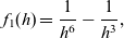 \begin{equation} f_1(h)=\frac{1}{h^6} -\frac{1}{h^3},\end{equation}
and
 \begin{equation}f_{\kern1pt{2}}(h) = \frac{1}{h^6},\end{equation}
i.e. we separate the spatially homogeneous and spatially non-homogeneous components of the disjoining pressure. Equation (A1) is subject to the periodic boundary conditions (5.7).
Suppose that when $\rho=0$
there is an orbit of steady-state solutions, i.e. a continuous closed curve of solutions
$\rho=0$
there is an orbit of steady-state solutions, i.e. a continuous closed curve of solutions $h_{0,s}(x)$
, parameterised by
$h_{0,s}(x)$
, parameterised by $s \in \mathbb{R}/[0,1]$
, such that
$s \in \mathbb{R}/[0,1]$
, such that $h_{0,s}(x):=h_0(x+s)$
, for some function
$h_{0,s}(x):=h_0(x+s)$
, for some function $h_0(x)$
, i.e. all these solutions are related by translation. We aim to understand what remains of this orbit for small non-zero
$h_0(x)$
, i.e. all these solutions are related by translation. We aim to understand what remains of this orbit for small non-zero $\rho$
.
$\rho$
.
Fix $s \in \mathbb{R}/[0,1]$
. We write
$s \in \mathbb{R}/[0,1]$
. We write
 \begin{equation}h(x)= h_{0,s}(x)+ \rho h_1(x) + O(\rho^2).\end{equation}
Substituting this expansion into (A1) and collecting the $O(\rho)$
terms, we have
$O(\rho)$
terms, we have
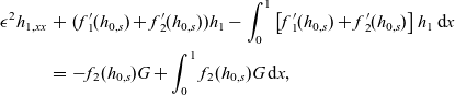 \begin{eqnarray} \epsilon^2 h_{1,xx} & + & ({f\kern0.5pt}_1{\kern0.5pt\!\!'}(h_{0,s})+{f\kern0.5pt}_2{\kern0.5pt\!\!'}(h_{0,s}))h_1 - \int_0^1 \left[{f\kern0.5pt}_1{\kern0.5pt\!\!'}(h_{0,s}) + {f\kern0.5pt}_2{\kern0.5pt\!\!'}(h_{0,s})\right] h_1 \, \hbox{d}{x} \nonumber \\ & = & - f_{\kern1pt{2}}(h_{0,s})G + \int_0^1 f_{\kern1pt{2}}(h_{0,s})G \, \hbox{d}{x},\end{eqnarray}
where, just like $h_{0,s}(x)$
,
$h_{0,s}(x)$
, $h_1(x)$
also satisfies the periodic boundary conditions (5.7).
$h_1(x)$
also satisfies the periodic boundary conditions (5.7).
Now set
 \begin{equation}K u := \epsilon^2 u_{1,xx} + ({f\kern0.5pt}_1{\kern0.5pt\!\!'}(h_{0,s})+{f\kern0.5pt}_2{\kern0.5pt\!\!'}(h_{0,s}))u - \int_0^1 [{f\kern0.5pt}_1{\kern0.5pt\!\!'}(h_{0,s}) + {f\kern0.5pt}_2{\kern0.5pt\!\!'}(h_{0,s})] u \, \hbox{d}{x},\end{equation}
and let D(K), the domain of K, be
 \begin{equation} D(K) = \left\{f \in C^2\left(\left[0,1\right]\right) \; | \, f(0)=f(1), f'(0)=f'(1)\right\}.\end{equation}
The operator K is self-adjoint with respect to the $L^2([0,1])$
inner product. Invoking the Fredholm Alternative [32, Theorem 7.26], we conclude that (A5) has 1-periodic solutions if and only if the right-hand side of (A5) is orthogonal in
$L^2([0,1])$
inner product. Invoking the Fredholm Alternative [32, Theorem 7.26], we conclude that (A5) has 1-periodic solutions if and only if the right-hand side of (A5) is orthogonal in $L^2([0,1])$
to the solutions of
$L^2([0,1])$
to the solutions of $Ku=0$
.
$Ku=0$
.
Next, we show that $u:= h_{0,s\!\!\!\!\!}'\;\;$
solves
$u:= h_{0,s\!\!\!\!\!}'\;\;$
solves $Ku=0$
. Indeed, by differentiating (A1) with
$Ku=0$
. Indeed, by differentiating (A1) with $\rho=0$
with respect to x, we find that u solves the equation
$\rho=0$
with respect to x, we find that u solves the equation
 \begin{equation} \epsilon^2 u_{xx}+ ({f\kern0.5pt}_1{\kern0.5pt\!\!'}(h_{0,s}) + {f\kern0.5pt}_2{\kern0.5pt\!\!'}(h_{0,s}))u=0.\end{equation}
Integrating this equation over the interval [0,1], we have that
 \begin{equation}\int_0^1 ({f\kern0.5pt}_1{\kern0.5pt\!\!'}(h_{0,s}) + {f\kern0.5pt}_2{\kern0.5pt\!\!'}(h_{0,s}))u\, \hbox{d}{x} =0.\end{equation}
Hence
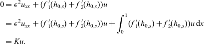 \begin{align}0 & = \epsilon^2 u_{xx}+ ({f\kern0.5pt}_1{\kern0.5pt\!\!'}(h_{0,s}) + {f\kern0.5pt}_2{\kern0.5pt\!\!'}(h_{0,s}))u \nonumber\\ & = \epsilon^2 u_{xx}+ ({f\kern0.5pt}_1{\kern0.5pt\!\!'}(h_{0,s}) + {f\kern0.5pt}_2{\kern0.5pt\!\!'}(h_{0,s}))u + \int_0^1 ({f\kern0.5pt}_1{\kern0.5pt\!\!'}(h_{0,s}) + {f\kern0.5pt}_2{\kern0.5pt\!\!'}(h_{0,s}))u\, \hbox{d}{x} \\ & = Ku. \nonumber\end{align}
Also note that as $h_{0,s}(x)$
satisfies periodic boundary conditions,
$h_{0,s}(x)$
satisfies periodic boundary conditions,
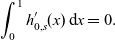 \begin{equation}\int_0^1 h_{0,s\!\!\!\!\!}'\;\;{\kern1pt}(x)\, \hbox{d}{x} = 0.\end{equation}
Hence the solvability condition for (A5) is
 \begin{equation} \int_0^1 h_{0,s\!\!\!\!\!}'\;\;{\kern1pt}(r)\left[ -f_{\kern1pt{2}}(h_{0,s})G + \int_0^1 f_{\kern1pt{2}}(h_{0,s})G \, \hbox{d}{x} \right] \hbox{d}{r} =0.\end{equation}
By (A11), this condition reduces to
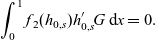 \begin{equation}\int_0^1 f_{\kern1pt{2}}(h_{0,s})h_{0,s\!\!\!\!\!}'\;\; {\kern1pt}G \, \hbox{d}{x} =0.\end{equation}
Now recall that $h_{0,s}(x) = h_0(x+s)$
, so if we write
$h_{0,s}(x) = h_0(x+s)$
, so if we write $F(x+s) = f_{\kern1pt{2}}(h_0(x+s))h_{0\!\!}'\kern1pt(x+s)$
, the function
$F(x+s) = f_{\kern1pt{2}}(h_0(x+s))h_{0\!\!}'\kern1pt(x+s)$
, the function $F(\cdot)$
is 1-periodic in x with zero mean. Hence
$F(\cdot)$
is 1-periodic in x with zero mean. Hence
 \begin{equation}F(z)= \sum_{k=1}^\infty \alpha_k \sin (2k\pi z) +\beta_k \cos (2k\pi z).\end{equation}
Therefore for $G(x)=\sin(2 \pi x)$
, the solvability condition for (A5) becomes
$G(x)=\sin(2 \pi x)$
, the solvability condition for (A5) becomes
 \begin{equation}\alpha_1 \sin (2k\pi s)-\beta_1 \cos(2\pi s)=0,\end{equation}
which has two solutions $ s \in \mathbb{R}/[0,1]$
, from which we conclude there is a solution
$ s \in \mathbb{R}/[0,1]$
, from which we conclude there is a solution $h_1(x)$
only for two choices of
$h_1(x)$
only for two choices of $s \in \mathbb{R}/[0,1]$
, that is, that only two solutions to (A1) remain from the entire O(2) orbit that exists for
$s \in \mathbb{R}/[0,1]$
, that is, that only two solutions to (A1) remain from the entire O(2) orbit that exists for $\rho=0$
.
$\rho=0$
.


 Open access

