


1 Introduction
Turbomachinery noise remains a significant contributor to overall aero-engine noise (Peake & Parry Reference Peake and Parry2012). A considerable source of broadband noise is the so-called ‘rotor–stator interaction’, where unsteady wakes shed by compressor rotors interact with downstream stators. Much progress has been made in understanding rotor–stator interaction noise when the blades are modelled as flat plates (Peake Reference Peake1992; Glegg Reference Glegg1999; Posson, Roger & Moreau Reference Posson, Roger and Moreau2010; Bouley et al. Reference Bouley, François, Roger, Posson and Moreau2017) or with realistic geometries (Evers & Peake Reference Evers and Peake2002; Baddoo & Ayton Reference Baddoo and Ayton2020). However, research into blades with complex boundaries – where the blades are not necessarily impermeable and rigid – is far less developed, especially from an analytic standpoint. This paper presents the first analytic treatment of scattering by cascades with complex boundary conditions, including compliance, porosity and impedance.
Aspirations for lighter and more efficient engines have driven the design of thinner and lighter blades in turbomachinery (Saiz Reference Saiz2008). As a result, aeroelastic effects such as flutter and resonance must be considered in modern turbomachinery design and testing (Hall, Kielb & Thomas Reference Hall, Kielb and Thomas2006). The rapid and accurate prediction of the aeroacoustic performance of turbomachinery with consideration of aeroelastic effects is therefore essential in evaluating the appropriateness of potential blade designs. Analytic solutions are excellent candidates for this task (Peake Reference Peake1992; Glegg Reference Glegg1999; Posson et al. Reference Posson, Roger and Moreau2010), but are presently limited to impermeable and rigid blades with no consideration of aeroelastic effects. The present study permits the consideration of compliant blades (Crighton & Leppington Reference Crighton and Leppington1970), where the blade deforms with a (purely) local response to the pressure gradient across the blade and elastic restoring forces are ignored. This is particularly relevant to marine applications where inertial effects dominate elastic restoring forces and our solution is an important first step towards modelling more general linearised elastic blades (Cavalieri, Wolf & Jaworski Reference Cavalieri, Wolf and Jaworski2016).
An influential trend in aeroacoustic research is to modify aerofoils with noise reducing technologies. A popular choice is a poroelastic extension, which was originally inspired by the silent flight of owls (Graham Reference Graham1934), and the corresponding experimental support of Geyer, Sarradj & Fritzsche (Reference Geyer, Sarradj and Fritzsche2010). A detailed review of research into the silent flight of owls is available in Jaworski & Peake (Reference Jaworski and Peake2020). Poroelastic extensions have been applied to semi-infinite (Jaworski & Peake Reference Jaworski and Peake2013) and finite (Ayton Reference Ayton2016) blades and have demonstrated considerable noise reductions. Structural requirements limit the application of highly porous blades in turbomachinery, but there remains the possibility that significant noise reductions are available for modest porosity values. The approach of the present research permits porous blades through the assumption of an impedance condition where the seepage velocity through the blade is proportional to the pressure jump across the blade. We will also consider the more general situation of an impedance relation along the blades (Myers Reference Myers1980).
In this paper we extend the analyses of Glegg (Reference Glegg1999) and Posson et al. (Reference Posson, Roger and Moreau2010) to analyse the scattering by a cascade of blades with a range of boundary conditions. The problem is solved with tools from complex variable theory, particularly the Wiener–Hopf method. Taking a Fourier transform maps the problem into the spectral plane where the Wiener–Hopf analysis is carried out in a similar way to Glegg (Reference Glegg1999). An inverse Fourier transform is applied to return the problem to physical space, and contour integration is applied to recover the acoustic field (Posson et al. Reference Posson, Roger and Moreau2010). A significant advantage of the presented technique is that the method is identical regardless of the boundary condition – the only effects of modifying the boundary condition are to modify the kernel in the Wiener–Hopf method.
A striking feature of the analysis is that modifications to the boundary conditions do not affect the modal structure of the solution in the far field. We arrive at this result by interrogating the (meromorphic) Wiener–Hopf kernel, which takes an interpretable form amenable to asymptotic and numerical analysis. We show that, in the spectral plane, the only effect of modifying the blade boundary condition is to vary the locations of the zeros of this Wiener–Hopf kernel, which corresponds to perturbing the duct modes of the cascade response function. Modifying the zeros has a significant effect on the acoustic field in the inter-blade region, in part because the cut-on frequencies of the duct modes are changed to account for energy being absorbed or produced by the blades. In fact, we will show that, in the case where the blades are porous, the duct modes are never cut-on. The poles of the Wiener–Hopf kernel correspond to the acoustic modes scattered into the far field and are invariant under modifications to the boundary conditions; the modes are a function of the cascade spacing and incident field alone. Consequently, the cut-on frequencies of the acoustic modes are unchanged and the modal structure of the upstream and downstream acoustic fields are the same regardless of boundary condition, although the coefficients of these modes do change, thus permitting a far-field noise reduction.
Our analysis is focussed on unloaded flat plates, although it is well known that loaded blades have a significant effect on aeroacoustic performance (Fang & Atassi Reference Fang and Atassi1993; Evers & Peake Reference Evers and Peake2002; Hall et al. Reference Hall, Kielb and Thomas2006). The present work could be merged with our recent solution for scattering by loaded cascades (Baddoo & Ayton Reference Baddoo and Ayton2020) to account for both the effects of complex boundary conditions and non-trivial geometries.
In the present study we consider four possible boundary conditions for the cascade blades, labelled cases 0–III. Physically, case 0 corresponds to rigid and impermeable blades; case I, porous or compliant blades with no background flow; case II, porous blades with background flow; and case III, a general impedance relation. Mathematically, case 0 corresponds to a Neumann boundary condition; case I, a Robin boundary condition; case II, an oblique derivative boundary condition; and case III, a generalised Cauchy boundary condition.
We begin by presenting a mathematical model for the cascade in § 2, including the modelling of the various boundary conditions. We then present some details of the mathematical solution in § 3. In § 4 we conduct a detailed investigation of the effects of blade porosity. In particular, we present a range of results on sound generation and sound transmission. Finally, in § 5 we summarise our work and suggest future directions of research. The code used to produce all the results is available at https://github.com/baddoo/complex-cascade-scattering.
2 Mathematical formulation
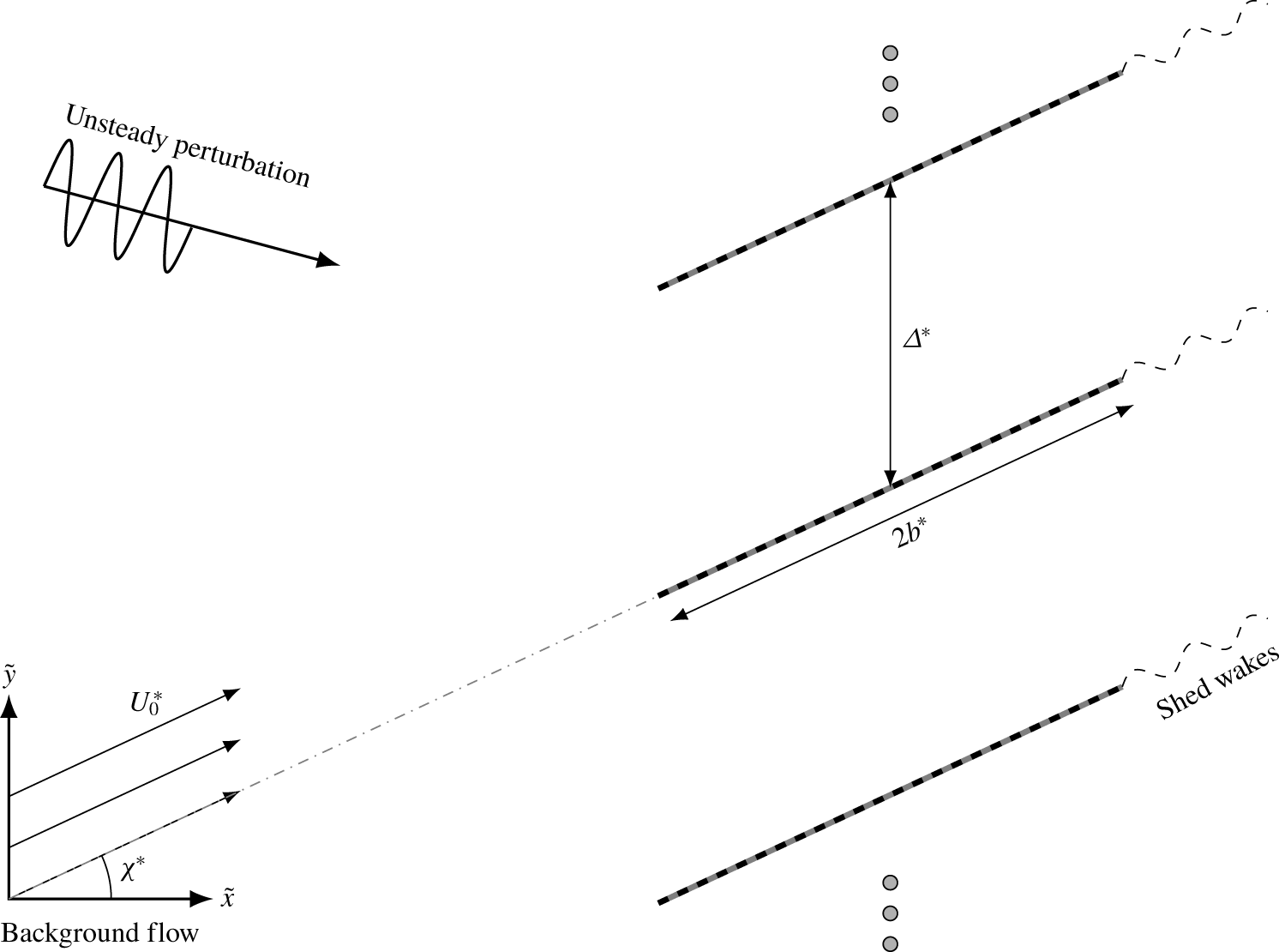
We consider a rectilinear cascade of blades in a uniform, subsonic flow as illustrated in figure 1. It is useful to rotate the coordinate system and define
 $$\begin{eqnarray}\displaystyle (x^{\ast },y^{\ast },z^{\ast })=(\tilde{x}\cos (\unicode[STIX]{x1D712}^{\ast })+{\tilde{y}}\sin (\unicode[STIX]{x1D712}^{\ast }),-\tilde{x}\sin (\unicode[STIX]{x1D712}^{\ast })+{\tilde{y}}\cos (\unicode[STIX]{x1D712}^{\ast }),\tilde{z}), & & \displaystyle \nonumber\end{eqnarray}$$
 so that the  $x^{\ast }$ and $y^{\ast }$ coordinates are tangential and normal to the blades respectively, which have dimensional length $2b^{\ast }$. The blades are unloaded, but we do permit a background flow tangential to the blades. Additionally, the background flow may have a spanwise component such that
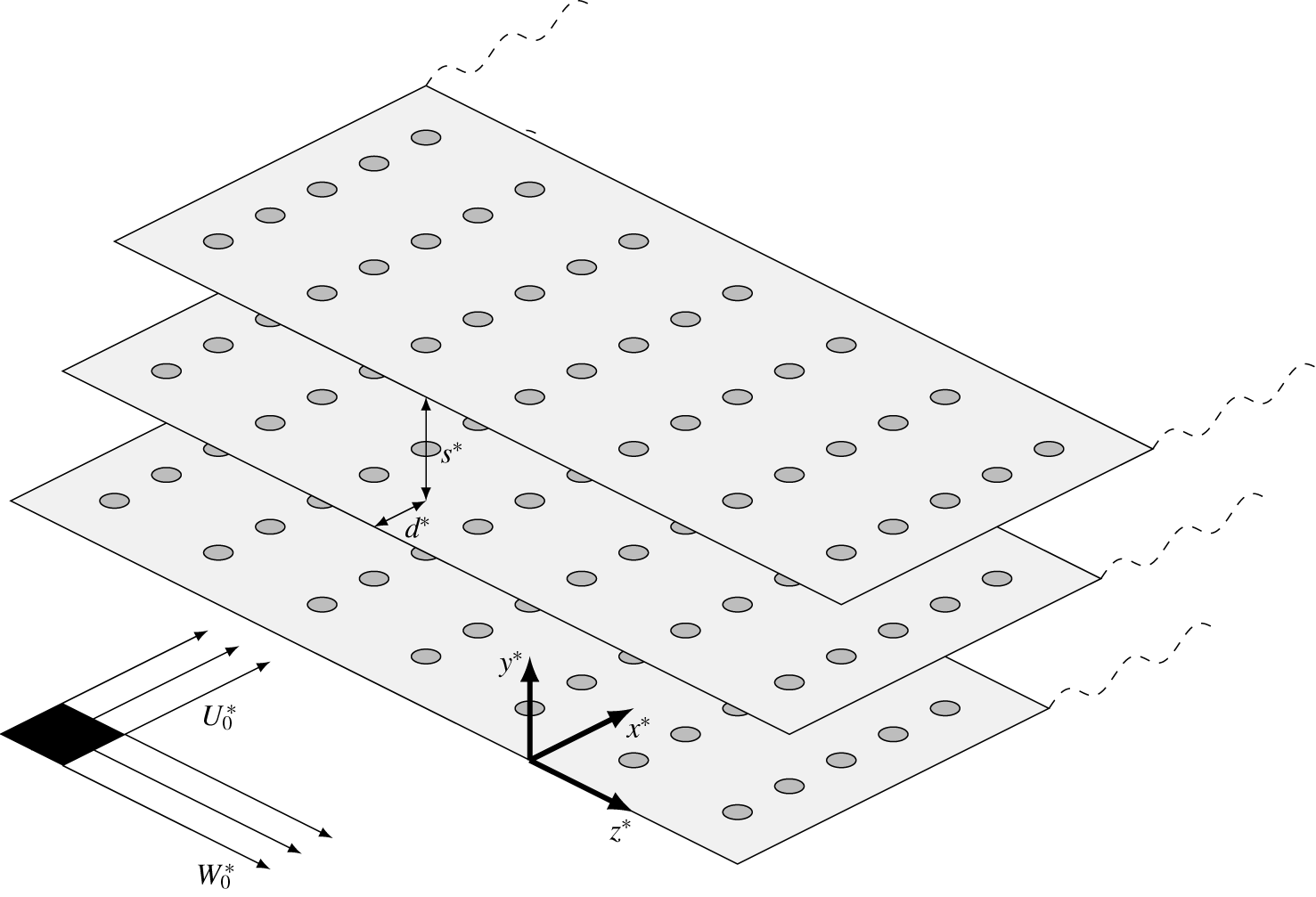
  $\boldsymbol{U}_{0}^{\ast }=(U_{0}^{\ast },0,W_{0}^{\ast })$, as illustrated in figure 2. The blades in the cascade are inclined at stagger angle $\unicode[STIX]{x1D712}^{\ast }$, and the distance between adjacent blades is $\unicode[STIX]{x1D6E5}^{\ast }$. Consequently, the spacing between blades is given by
 $$\begin{eqnarray}\displaystyle (d^{\ast },s^{\ast })=\unicode[STIX]{x1D6E5}^{\ast }(\sin (\unicode[STIX]{x1D712}^{\ast }),\cos (\unicode[STIX]{x1D712}^{\ast })). & & \displaystyle \nonumber\end{eqnarray}$$
 We assume, as it is often the case in practical scenarios, that the blades are staggered and overlapping i.e.  $0<d^{\ast }<2b^{\ast }$. The case of non-overlapping blades could be treated in a similar fashion to Maierhofer & Peake (Reference Maierhofer and Peake2020). The zero-stagger arrangement can be recovered as a degenerate case of our results. We further assume that a vortical or acoustic wave is incident on the cascade, resulting in a velocity perturbation $\boldsymbol{u}^{\ast }$ to the mean flow. The Kutta condition is satisfied by ensuring that there is no pressure jump at the blades’ trailing edges, and the pressure singularity at the leading edge is restricted to be integrable.
An infinite, rectilinear cascade of flat plates with complex boundary conditions subjected to an unsteady perturbation. The plates have dimensional length  $2b^{\ast }$ and are inclined at a stagger angle of $\unicode[STIX]{x1D712}^{\ast }$. The plates produce an unsteady wake in the case where there is a non-zero chordwise background flow $U_{0}^{\ast }$.
A three-dimensional view of the cascade in the rotated, dimensional  $(x^{\ast },y^{\ast },z^{\ast })$ coordinate system. The background velocities may have a spanwise component $W_{0}^{\ast }$. The complex boundaries are illustrated by the holes on each blade, which may represent compliance, porosity or impedance.
We introduce an acoustic potential function for the scattered field defined by
 $$\begin{eqnarray}\displaystyle \unicode[STIX]{x1D735}\unicode[STIX]{x1D719}^{\ast }=\boldsymbol{u}^{\ast }. & & \displaystyle \nonumber\end{eqnarray}$$
Consequently, conservation of momentum gives the scattered pressure as
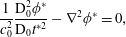
 $$\begin{eqnarray}\displaystyle p^{\ast }=-\unicode[STIX]{x1D70C}_{0}^{\ast }\frac{\text{D}_{0}\unicode[STIX]{x1D719}^{\ast }}{\text{D}_{0}t^{\ast }}, & & \displaystyle\end{eqnarray}$$
 where  $\unicode[STIX]{x1D70C}_{0}^{\ast }$ is the mean flow density and the (linearised) convective derivative is defined as
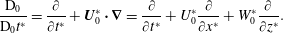 $$\begin{eqnarray}\displaystyle \frac{\text{D}_{0}}{\text{D}_{0}t^{\ast }}=\frac{\unicode[STIX]{x2202}}{\unicode[STIX]{x2202}t^{\ast }}+\boldsymbol{U}_{0}^{\ast }\boldsymbol{\cdot }\unicode[STIX]{x1D735}=\frac{\unicode[STIX]{x2202}}{\unicode[STIX]{x2202}t^{\ast }}+U_{0}^{\ast }\frac{\unicode[STIX]{x2202}}{\unicode[STIX]{x2202}x^{\ast }}+W_{0}^{\ast }\frac{\unicode[STIX]{x2202}}{\unicode[STIX]{x2202}z^{\ast }}. & & \displaystyle \nonumber\end{eqnarray}$$
Accordingly, conservation of mass gives the convected wave equation
 $$\begin{eqnarray}\displaystyle \frac{1}{c_{0}^{2}}\frac{\text{D}_{0}^{2}\unicode[STIX]{x1D719}^{\ast }}{\text{D}_{0}t^{\ast 2}}-\unicode[STIX]{x1D6FB}^{2}\unicode[STIX]{x1D719}^{\ast }=0, & & \displaystyle\end{eqnarray}$$
 where  $c_{0}$ is the isentropic speed of sound.
We suppose that the unsteady perturbation incident on the cascade takes the form
 $$\begin{eqnarray}\displaystyle \unicode[STIX]{x1D719}_{i}^{\ast }=\exp [\text{i}(k_{x}^{\ast }x^{\ast }+k_{y}^{\ast }y^{\ast }+k_{z}^{\ast }z^{\ast }-\unicode[STIX]{x1D714}^{\ast }t^{\ast })]. & & \displaystyle\end{eqnarray}$$
 Dimensional variables are denoted with  $\ast$ whereas non-dimensional variables have no annotation. Since the system is infinite in the spanwise direction, the scattered solution $\boldsymbol{u}^{\ast }$ must also have harmonic dependence in the $z^{\ast }$-direction. Accordingly, making the following convective transformation and non-dimensionalisations
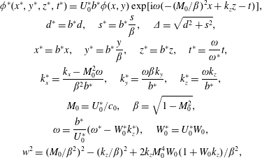 $$\begin{eqnarray}\displaystyle & \displaystyle \unicode[STIX]{x1D719}^{\ast }(x^{\ast },y^{\ast },z^{\ast },t^{\ast })=U_{0}^{\ast }b^{\ast }\unicode[STIX]{x1D719}(x,y)\exp [\text{i}\unicode[STIX]{x1D714}(-(M_{0}/\unicode[STIX]{x1D6FD})^{2}x+k_{z}z-t)], & \displaystyle \nonumber\\ \displaystyle & \displaystyle d^{\ast }=b^{\ast }d,\quad s^{\ast }=b^{\ast }\frac{s}{\unicode[STIX]{x1D6FD}},\quad \unicode[STIX]{x1D6E5}=\sqrt{d^{2}+s^{2}}, & \displaystyle \nonumber\\ \displaystyle & \displaystyle x^{\ast }=b^{\ast }x,\quad y^{\ast }=b^{\ast }\frac{y}{\unicode[STIX]{x1D6FD}},\quad z^{\ast }=b^{\ast }z,\quad t^{\ast }=\frac{\unicode[STIX]{x1D714}}{\unicode[STIX]{x1D714}^{\ast }}t, & \displaystyle \nonumber\\ \displaystyle & \displaystyle k_{x}^{\ast }=\frac{k_{x}-M_{0}^{2}\unicode[STIX]{x1D714}}{\unicode[STIX]{x1D6FD}^{2}b^{\ast }},\quad k_{y}^{\ast }=\frac{\unicode[STIX]{x1D714}\unicode[STIX]{x1D6FD}k_{y}}{b^{\ast }},\quad k_{z}^{\ast }=\frac{\unicode[STIX]{x1D714}k_{z}}{b^{\ast }}, & \displaystyle \nonumber\\ \displaystyle & \displaystyle M_{0}=U_{0}^{\ast }/c_{0},\quad \unicode[STIX]{x1D6FD}=\sqrt{1-M_{0}^{2}}, & \displaystyle \nonumber\\ \displaystyle & \displaystyle \unicode[STIX]{x1D714}=\frac{b^{\ast }}{U_{0}^{\ast }}(\unicode[STIX]{x1D714}^{\ast }-W_{0}^{\ast }k_{z}^{\ast }),\quad W_{0}^{\ast }=U_{0}^{\ast }W_{0}, & \displaystyle \nonumber\\ \displaystyle & \displaystyle w^{2}=(M_{0}/\unicode[STIX]{x1D6FD}^{2})^{2}-(k_{z}/\unicode[STIX]{x1D6FD})^{2}+2k_{z}M_{0}^{4}W_{0}(1+W_{0}k_{z})/\unicode[STIX]{x1D6FD}^{2}, & \displaystyle \nonumber\end{eqnarray}$$
reduces (2.2) to
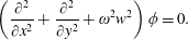 $$\begin{eqnarray}\displaystyle \left(\frac{\unicode[STIX]{x2202}^{2}}{\unicode[STIX]{x2202}x^{2}}+\frac{\unicode[STIX]{x2202}^{2}}{\unicode[STIX]{x2202}y^{2}}+\unicode[STIX]{x1D714}^{2}w^{2}\right)\unicode[STIX]{x1D719}=0. & & \displaystyle\end{eqnarray}$$
 An alternative non-dimensionalisation is required when  $U_{0}^{\ast }=0$, but this is a trivial modification. In terms of these new variables, the scattered pressure (2.1) becomes
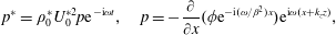 $$\begin{eqnarray}\displaystyle p^{\ast }=\unicode[STIX]{x1D70C}_{0}^{\ast }U_{0}^{\ast 2}p\text{e}^{-\text{i}\unicode[STIX]{x1D714}t},\quad p=-\frac{\unicode[STIX]{x2202}}{\unicode[STIX]{x2202}x}(\unicode[STIX]{x1D719}\text{e}^{-\text{i}(\unicode[STIX]{x1D714}/\unicode[STIX]{x1D6FD}^{2})x})\text{e}^{\text{i}\unicode[STIX]{x1D714}(x+k_{z}z)}, & & \displaystyle\end{eqnarray}$$
 where  $p$ is the non-dimensional pressure, and the incident perturbation becomes
 $$\begin{eqnarray}\displaystyle \unicode[STIX]{x1D719}_{i}^{\ast }=U_{0}^{\ast }b^{\ast }\unicode[STIX]{x1D719}_{i}(x,y)\text{e}^{\text{i}\unicode[STIX]{x1D714}(-(M_{0}/\unicode[STIX]{x1D6FD})^{2}x+k_{z}z-t)},\quad \unicode[STIX]{x1D719}_{i}=\exp [\text{i}((k_{x}/\unicode[STIX]{x1D6FD}^{2})x+\unicode[STIX]{x1D714}k_{y}y)]. & & \displaystyle\end{eqnarray}$$
2.1 Boundary conditions
We now introduce the boundary conditions for the problem. It is sufficient to specify the behaviour along  $y=ns^{\pm }$ for $n\in \mathbb{Z}$. We use $\unicode[STIX]{x1D6E5}_{n}[f]$ and $\unicode[STIX]{x1D6F4}_{n}[f]$ respectively to denote the difference and sum of $f$ either side of the $n$th blade or wake.
2.1.1 Upstream boundary condition
There may be no discontinuities upstream of the blade row. Consequently, we write
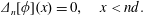 $$\begin{eqnarray}\displaystyle \unicode[STIX]{x1D6E5}_{n}[\unicode[STIX]{x1D719}](x)=0,\quad x<nd. & & \displaystyle\end{eqnarray}$$
2.1.2 Blade surface boundary conditions
We now introduce several possible blade surface boundary conditions that can be modelled with our solution. The types of blades we consider are the classical impermeable and rigid blade, a porous or compliant blade without background flow, a porous blade with background flow and a blade with a general impedance condition. All these blades admit closed-form, homogenised boundary conditions that are relatively simple to express. Moreover, all the boundary conditions take the same form. By solving for all possibly boundary condition simultaneously, we are able to model a range of scenarios of practical interest without modifying our solution. As we shall see later, the effect of modifying the boundary condition is to modify the kernel in the ensuing Wiener–Hopf analysis.
In this initial study, we focus on boundary conditions that are locally reacting so that the sound propagation at a given point on or inside the blade depends only on the acoustic pressure above and below that point. Accordingly, the surface impedance does not depend on the angle of the incident wave. For example, in the case of porous blades, we consider blades that can be characterised by lattices of unconnected, straight pores. In contrast, the sound field inside a connected pore will depend on the sound field in the neighbouring pores in addition to the sound pressure above and below the pore. The effects of non-locally reacting boundary conditions could, in principle, be considered by our solution if the corresponding boundary conditions can be homogenised for the infinitesimal blades that we consider. Additionally, we assume that the impedance is the same at all points on the blade e.g. the porosity is constant in both the chordwise and spanwise directions.
We now summarise the different types of boundary conditions that may be considered.
Case 0
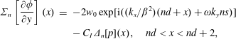
When the blade is rigid and impermeable, the no-flux condition is simply
 $$\begin{eqnarray}\displaystyle \boldsymbol{u}_{T}\boldsymbol{\cdot }\boldsymbol{n}=0,\quad nd<x<nd+2,y=ns^{\pm }, & & \displaystyle\end{eqnarray}$$
 where  $\boldsymbol{n}$ is the normal vector directed away from the blade and $\boldsymbol{u}_{T}$ denotes the total (incident and scattered) velocity field. We sum the contributions of (2.8) either side of each blade to obtain
 $$\begin{eqnarray}\displaystyle \unicode[STIX]{x1D6F4}_{n}\left[\frac{\unicode[STIX]{x2202}\unicode[STIX]{x1D719}}{\unicode[STIX]{x2202}y}\right](x)=-2w_{0}\exp [\text{i}((k_{x}/\unicode[STIX]{x1D6FD}^{2})(nd+x)+\unicode[STIX]{x1D714}k_{y}ns)],\quad nd<x<nd+2, & & \displaystyle\end{eqnarray}$$
 where  $w_{0}=\text{i}\unicode[STIX]{x1D714}k_{y}$ is the non-dimensional amplitude of the normal velocity of the incident perturbation on the 0th blade. This case has been considered in detail in previous research (Glegg Reference Glegg1999; Posson et al. Reference Posson, Roger and Moreau2010) and is therefore not considered further in the present work.
Case I
We now consider blades with perforations such as the circular apertures illustrated in figure 2. For a pressure load of frequency  $\unicode[STIX]{x1D714}$, the Rayleigh conductivity $K_{R}$ relates the mass per unit time ( $Q$) flowing through an isolated aperture to the pressure difference either side of the aperture ( $p^{+}-p^{-}$) by (Strutt Reference Strutt1870)
 $$\begin{eqnarray}\displaystyle K_{R}=\frac{\text{i}\unicode[STIX]{x1D714}Q}{p^{+}-p^{-}}, & & \displaystyle\end{eqnarray}$$
 in our non-dimensional variables. The Rayleigh conductivity is a function of the aperture shape:  $K_{R}=2R$ for a circular aperture of radius $R$ in a zero-thickness plate. Recently, Brandão & Schnitzer (Reference Brandão and Schnitzer2020) derived asymptotic expressions for the Rayleigh conductivity of a cylindrical orifice in a plate of finite thickness. These solutions also account for the viscous effects of a Stokes boundary later adjacent to the plate. A thorough discussion of the Rayleigh conductivity may be found in § 5.3.1 of Howe (Reference Howe1998).
The Rayleigh conductivity (2.10) can be deployed to derive an effective condition for a blade with multiple apertures through a homogenisation procedure. Suppose that the blade has  $N$ perforations per unit area, each of conductivity $K_{R}$. Assuming that the acoustic wavelength is large compared to the aperture size, the pressure either side can be regarded as constant over the aperture length. If the apertures are sufficiently far apart, their conductivity can be measured as if they were in isolation. Therefore, (2.10) holds on the aperture scale and each aperture contributes a mass flux of $Q$. Consequently, the total mass flux per unit area is $NQ=NK_{R}(p^{+}-p^{-})/(\text{i}\unicode[STIX]{x1D714})$ which must match with $v_{T}$ by continuity, where $v_{T}$ is the total velocity in the $y$-direction. Accordingly, we may simply write the effective conductivity $\tilde{K}_{R}$ for a plate with $N$ apertures per unit area with conductivity $K_{R}$ as $\tilde{K}_{R}=NK_{R}$. This argument has been made rigorous by Bendali et al. (Reference Bendali, Fares, Piot and Tordeux2013). In the case of circular apertures of radius $R$, the effective conductivity becomes
 $$\begin{eqnarray}\displaystyle \tilde{K}_{R}=\frac{2\unicode[STIX]{x1D6FC}_{H}}{\unicode[STIX]{x03C0}R}, & & \displaystyle \nonumber\end{eqnarray}$$
 for fractional open area  $\unicode[STIX]{x1D6FC}_{H}$.
Substituting our flow variables into (2.10), we generalise the no-flux condition (2.8) and obtain
 $$\begin{eqnarray}\displaystyle v_{T}=\frac{\tilde{K}_{R}}{\text{i}\unicode[STIX]{x1D714}}\unicode[STIX]{x1D6E5}_{n}[p](x),\quad nd<x<nd+2,y=ns^{\pm }. & & \displaystyle\end{eqnarray}$$
Summing the contributions either side of the blade in (2.11) yields
 $$\begin{eqnarray}\displaystyle \unicode[STIX]{x1D6F4}_{n}\left[\frac{\unicode[STIX]{x2202}\unicode[STIX]{x1D719}}{\unicode[STIX]{x2202}y}\right](x) & = & \displaystyle -2w_{0}\exp [\text{i}((k_{x}/\unicode[STIX]{x1D6FD}^{2})(nd+x)+\unicode[STIX]{x1D714}k_{y}ns)]\nonumber\\ \displaystyle & & \displaystyle -\,C_{I}\unicode[STIX]{x1D6E5}_{n}[p](x),\quad nd<x<nd+2,\end{eqnarray}$$
 for constant  $C_{I}=-2\tilde{K}_{R}/(\text{i}\unicode[STIX]{x1D714})$. In the absence of background flow, this condition becomes (subject to an alternative non-dimensionalisation)
 $$\begin{eqnarray}\displaystyle \unicode[STIX]{x1D6F4}_{n}\left[\frac{\unicode[STIX]{x2202}\unicode[STIX]{x1D719}}{\unicode[STIX]{x2202}y}\right](x) & = & \displaystyle -2w_{0}\exp [\text{i}((k_{x}/\unicode[STIX]{x1D6FD}^{2})(nd+x)+\unicode[STIX]{x1D714}k_{y}ns)]\nonumber\\ \displaystyle & & \displaystyle +\,C_{I}\unicode[STIX]{x1D6E5}_{n}[\unicode[STIX]{x1D719}](x),\quad nd<x<nd+2.\end{eqnarray}$$
 This boundary condition has gained popularity as a tool for analysing the aerodynamic scattering of porous edges (Jaworski & Peake Reference Jaworski and Peake2013; Ayton Reference Ayton2016; Kisil & Ayton Reference Kisil and Ayton2018), but it is also valid in other scenarios: Leppington (Reference Leppington1977) showed that (2.13) is equivalent to the boundary condition for an impermeable, compliant plate. Indeed, Crighton & Leppington (Reference Crighton and Leppington1970) used (2.13) to analyse the scattering of aerodynamic sound by a semi-infinite compliant plate. In that study, the plate was modelled as possessing inertia, but negligible elastic resistance to deformation. Consequently, the pressure difference across the compliant plate was proportional to the specific mass of the plate multiplied by the acceleration so that, in the notation of the present work, the constant  $C_{I}$ would instead become $C_{I}=-2/m$ where $m$ is the (non-dimensional) mass of the plate per unit area.
Case II
We now consider the case where the plates are porous and embedded in a mean flow. The mean flow has a significant effect on the Rayleigh conductivity for an aperture, and analytic expressions for  $K_{R}$ are generally intractable. However, Howe, Scott & Sipcic (Reference Howe, Scott and Sipcic1996) showed that, for a circular aperture in a grazing flow, the Rayleigh conductivity is
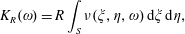 $$\begin{eqnarray}\displaystyle K_{R}(\unicode[STIX]{x1D714})=R\int _{S}\unicode[STIX]{x1D708}(\unicode[STIX]{x1D709},\unicode[STIX]{x1D702},\unicode[STIX]{x1D714})\,\text{d}\unicode[STIX]{x1D709}\,\text{d}\unicode[STIX]{x1D702}, & & \displaystyle\end{eqnarray}$$
 where the integral is taken over the aperture area ( $\unicode[STIX]{x1D709}^{2}+\unicode[STIX]{x1D702}^{2}<R^{2}$). The function $\unicode[STIX]{x1D708}(\unicode[STIX]{x1D709},\unicode[STIX]{x1D702},\unicode[STIX]{x1D714})$ corresponds to the displacement of fluid at the aperture interface and must be found as the solution to an integral equation defined in Howe et al. (Reference Howe, Scott and Sipcic1996). This equation must generally be solved numerically and a range of values for $K_{R}(\unicode[STIX]{x1D714})$ are recorded in table 2 of Howe et al. (Reference Howe, Scott and Sipcic1996). Unlike case I boundary conditions, the conductivity may be complex so it is convenient to separate the complex conductivity into real and imaginary parts
 $$\begin{eqnarray}\displaystyle K_{R}(\unicode[STIX]{x1D714})=2R(\unicode[STIX]{x1D6E4}_{R}(\unicode[STIX]{x1D714})-\text{i}\unicode[STIX]{x1D6E5}_{R}(\unicode[STIX]{x1D714})), & & \displaystyle \nonumber\end{eqnarray}$$
 where  $\unicode[STIX]{x1D6E4}_{R}(\unicode[STIX]{x1D714})$ and $\unicode[STIX]{x1D6E5}_{R}(\unicode[STIX]{x1D714})$ are real valued functions of frequency. Using a similar argument to the previous section, we may write the effective compliance for a perforated plate as $\tilde{K}_{R}=NK_{R}$. The no-flux condition (2.8) now generalises to
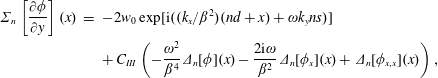
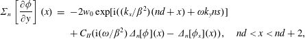 $$\begin{eqnarray}\displaystyle \unicode[STIX]{x1D6F4}_{n}\left[\frac{\unicode[STIX]{x2202}\unicode[STIX]{x1D719}}{\unicode[STIX]{x2202}y}\right](x) & = & \displaystyle -2w_{0}\exp [\text{i}((k_{x}/\unicode[STIX]{x1D6FD}^{2})(nd+x)+\unicode[STIX]{x1D714}k_{y}ns)]\nonumber\\ \displaystyle & & \displaystyle +\,C_{II}(\text{i}(\unicode[STIX]{x1D714}/\unicode[STIX]{x1D6FD}^{2})\unicode[STIX]{x1D6E5}_{n}[\unicode[STIX]{x1D719}](x)-\unicode[STIX]{x1D6E5}_{n}[\unicode[STIX]{x1D719}_{x}](x)),\quad nd<x<nd+2,\quad\end{eqnarray}$$
 where again  $C_{II}=2\tilde{K}_{R}(\unicode[STIX]{x1D714})/(\text{i}\unicode[STIX]{x1D714})$ is a constant.
Case III
We may also consider the effects of an impedance boundary condition. In the presence of background flow, the impedance boundary condition is given by Myers (Reference Myers1980)
 $$\begin{eqnarray}\displaystyle \boldsymbol{u}_{T}\boldsymbol{\cdot }\boldsymbol{n}=\left(\frac{\unicode[STIX]{x2202}}{\unicode[STIX]{x2202}t}+\boldsymbol{U}_{0}\boldsymbol{\cdot }\unicode[STIX]{x1D735}-\boldsymbol{n}\boldsymbol{\cdot }(\boldsymbol{n}\boldsymbol{\cdot }\unicode[STIX]{x1D735}\boldsymbol{U}_{0})\right)\frac{p}{\text{i}\unicode[STIX]{x1D714}Z}, & & \displaystyle \nonumber\end{eqnarray}$$
 where  $\boldsymbol{n}$ is now directed into the blade. The real part of the impedance $Z$ is termed the acoustic resistance and represents the energy transfer of the blade: if $\text{Re}[Z]>0$ then the blades absorb energy whereas if $\text{Re}[Z]<0$ then the blades produce energy. Since the flow is uniform, this condition applied on the upper and lower surfaces of the blades becomes, in terms of the present variables,
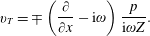 $$\begin{eqnarray}\displaystyle v_{T}=\mp \left(\frac{\unicode[STIX]{x2202}}{\unicode[STIX]{x2202}x}-\text{i}\unicode[STIX]{x1D714}\right)\frac{p}{\text{i}\unicode[STIX]{x1D714}Z}. & & \displaystyle \nonumber\end{eqnarray}$$
We now sum the upper and lower components of this impedance condition to obtain a condition on the sum of the velocity either side of the blade
 $$\begin{eqnarray}\displaystyle \unicode[STIX]{x1D6F4}_{n}\left[\frac{\unicode[STIX]{x2202}\unicode[STIX]{x1D719}}{\unicode[STIX]{x2202}y}\right](x) & = & \displaystyle -2w_{0}\exp [\text{i}((k_{x}/\unicode[STIX]{x1D6FD}^{2})(nd+x)+\unicode[STIX]{x1D714}k_{y}ns)]\nonumber\\ \displaystyle & & \displaystyle +\,C_{III}\left(-\frac{\unicode[STIX]{x1D714}^{2}}{\unicode[STIX]{x1D6FD}^{4}}\unicode[STIX]{x1D6E5}_{n}[\unicode[STIX]{x1D719}](x)-\frac{2\text{i}\unicode[STIX]{x1D714}}{\unicode[STIX]{x1D6FD}^{2}}\unicode[STIX]{x1D6E5}_{n}[\unicode[STIX]{x1D719}_{x}](x)+\unicode[STIX]{x1D6E5}_{n}[\unicode[STIX]{x1D719}_{x,x}](x)\right),\end{eqnarray}$$
 where  $C_{III}=1/(\text{i}\unicode[STIX]{x1D714}Z)$.
The presence of higher-order derivatives requires further regularity at the blades’ edges. Since the blades are fixed (and are only locally reacting), we additionally enforce that  $\unicode[STIX]{x1D6E5}_{n}[\unicode[STIX]{x1D719}_{x}](0)$ is bounded.
Summary of blade surface boundary conditions
We may characterise all the modified boundary conditions (2.13), (2.15) and (2.16) in the general form
 $$\begin{eqnarray}\displaystyle & & \displaystyle \unicode[STIX]{x1D6F4}_{n}\left[\frac{\unicode[STIX]{x2202}\unicode[STIX]{x1D719}}{\unicode[STIX]{x2202}y}\right](x)=-2w_{0}\exp [\text{i}((k_{x}/\unicode[STIX]{x1D6FD}^{2})(nd+x)+\unicode[STIX]{x1D714}k_{y}ns)]\nonumber\\ \displaystyle & & \displaystyle \qquad \quad +\,\unicode[STIX]{x1D707}_{0}\unicode[STIX]{x1D6E5}_{n}[\unicode[STIX]{x1D719}](x)+\unicode[STIX]{x1D707}_{1}\unicode[STIX]{x1D6E5}_{n}[\unicode[STIX]{x1D719}_{x}](x)+\unicode[STIX]{x1D707}_{2}\unicode[STIX]{x1D6E5}_{n}[\unicode[STIX]{x1D719}_{x,x}](x),\quad nd<x<nd+2,\quad\end{eqnarray}$$
 where the  $\unicode[STIX]{x1D707}_{n}$ are summarised in table 1 for the different boundary conditions. Furthermore, in the present analysis we do not allow any added mass generated in the blades and enforce that there is no jump in the normal velocity either side of the plate. Accordingly, we may write
 $$\begin{eqnarray}\displaystyle \unicode[STIX]{x1D6E5}_{n}\left[\frac{\unicode[STIX]{x2202}\unicode[STIX]{x1D719}}{\unicode[STIX]{x2202}y}\right](x)=0,\quad nd<x<nd+2. & & \displaystyle\end{eqnarray}$$
Summary of possible boundary conditions and corresponding  $\unicode[STIX]{x1D707}_{0}$, $\unicode[STIX]{x1D707}_{1}$ and $\unicode[STIX]{x1D707}_{2}$ values for (2.17). The references highlight relevant papers, although only [1,2] consider cascade geometries and are restricted to impermeable and rigid boundaries. The reference numbers correspond to [1] (Glegg Reference Glegg1999), [2] (Posson et al. Reference Posson, Roger and Moreau2010), [3] (Leppington Reference Leppington1977), [4] (Howe Reference Howe1998), [5] (Jaworski & Peake Reference Jaworski and Peake2013), [6] (Kisil & Ayton Reference Kisil and Ayton2018), [7] (Howe et al. Reference Howe, Scott and Sipcic1996), [8] (Myers Reference Myers1980) and [9] (Brambley Reference Brambley2009).

2.1.3 Downstream boundary conditions
Downstream, we require the pressure jump across the wake to vanish:
 $$\begin{eqnarray}\displaystyle \unicode[STIX]{x1D6E5}_{n}[p](x)=0,\quad x>2+nd. & & \displaystyle\end{eqnarray}$$
 By employing the pressure definition (2.5) and integrating with respect to  $x$, we may write the above condition as
 $$\begin{eqnarray}\displaystyle \unicode[STIX]{x1D6E5}_{n}[\unicode[STIX]{x1D719}](x)=2\unicode[STIX]{x03C0}\text{i}P\exp [\text{i}(\unicode[STIX]{x1D714}/\unicode[STIX]{x1D6FD}^{2})x],\quad x>nd+2, & & \displaystyle\end{eqnarray}$$
 where  $P$ is a constant of integration that will be specified by enforcing the Kutta condition.
Additionally, the normal velocity across the wake must vanish, i.e.
 $$\begin{eqnarray}\displaystyle \unicode[STIX]{x1D6E5}_{n}\left[\frac{\unicode[STIX]{x2202}\unicode[STIX]{x1D719}}{\unicode[STIX]{x2202}y}\right](x)=0,\quad x>nd+2. & & \displaystyle\end{eqnarray}$$
2.1.4 Summary of full boundary conditions
All in all, we have five boundary conditions. In the upstream region we do not permit any discontinuities (2.7). Along each blade we have a relation for the sum of normal velocities either side of the blade (2.17), and do not permit a jump in normal velocity across the blade (2.18). Finally, across the wake we do not permit a jump in pressure (2.20) or normal velocity (2.21). The boundary conditions are illustrated in figure 3. This completes the description of the mathematical model.
Schematic illustrating where each boundary condition is applied.

3 Solution
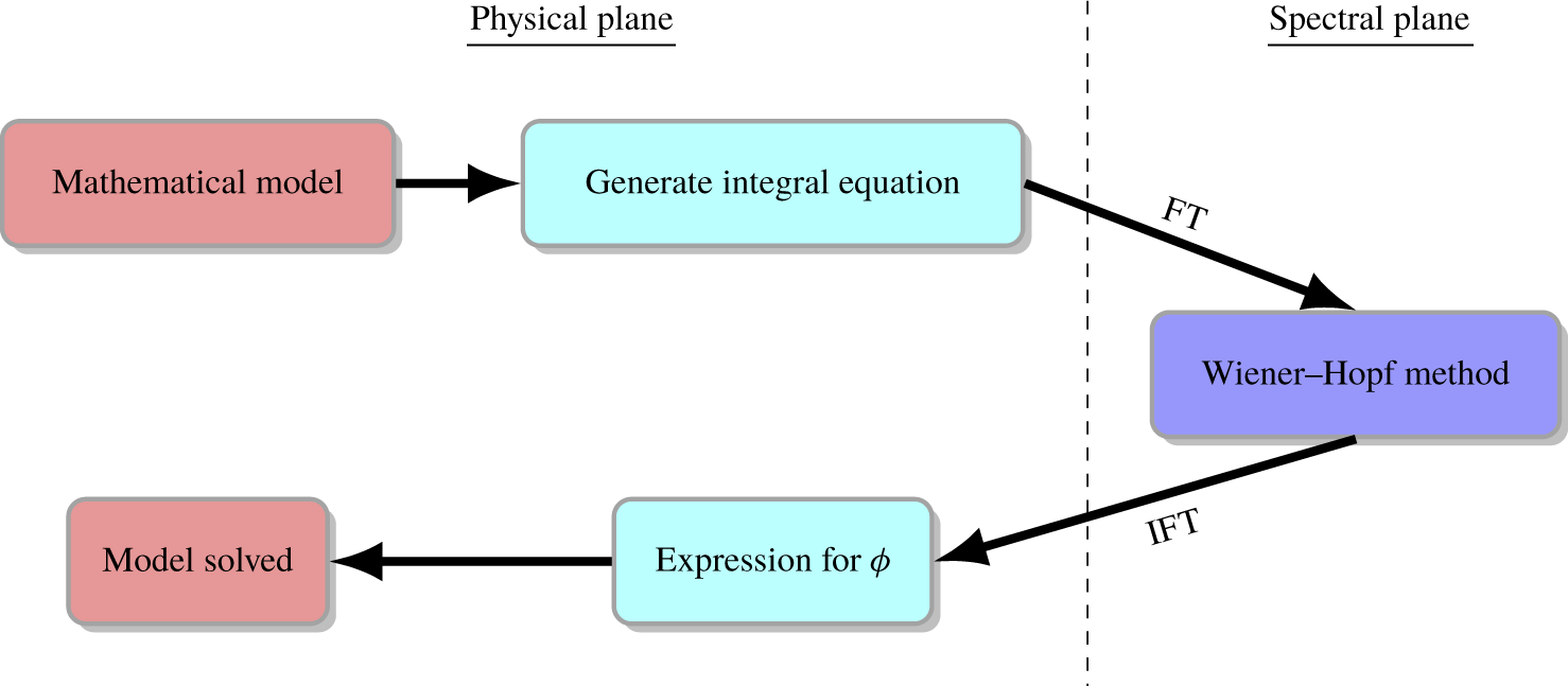
We now present the mathematical solution to the Helmholtz equation (2.4) subject to the boundary conditions (2.7), (2.17), (2.18), (2.20) and (2.21). For clarity, we present a ‘road map’ of the solution in figure 4. Further details of the solution procedure may be found in Baddoo & Ayton (Reference Baddoo and Ayton2020).
Schematic diagram illustrating the solution method. The abbreviations ‘FT’ and ‘IFT’ stand for ‘Fourier transform’ and ‘Inverse Fourier transform’ respectively.
As is typical in cascade acoustics problems we employ integral transforms to obtain a solution that is uniformly valid throughout the entire domain (Peake Reference Peake1992; Glegg Reference Glegg1999; Posson et al. Reference Posson, Roger and Moreau2010). However,  $\unicode[STIX]{x1D719}$ is discontinuous across each blade and wake in the $y$-direction. Therefore, $\unicode[STIX]{x2202}\unicode[STIX]{x1D719}/\unicode[STIX]{x2202}y$ possesses non-integrable singularities thus preventing the application of a Fourier transform. Consequently, we must regularise the derivatives of $\unicode[STIX]{x1D719}$ to remove these non-integrable singularities. To this end, we introduce introduce generalised derivatives (Lighthill Reference Lighthill1958) and write
 $$\begin{eqnarray}\displaystyle \frac{\unicode[STIX]{x2202}^{2}\unicode[STIX]{x1D719}}{\unicode[STIX]{x2202}y^{2}}=\frac{\tilde{\unicode[STIX]{x2202}}^{2}\unicode[STIX]{x1D719}}{\tilde{\unicode[STIX]{x2202}}y^{2}}-\mathop{\sum }_{n=-\infty }^{\infty }\unicode[STIX]{x1D6E5}_{n}[\unicode[STIX]{x1D719}](x)\unicode[STIX]{x1D6FF}^{\prime }(y-ns)-\mathop{\sum }_{n=-\infty }^{\infty }\unicode[STIX]{x1D6E5}_{n}\left[\frac{\unicode[STIX]{x2202}\unicode[STIX]{x1D719}}{\unicode[STIX]{x2202}y}\right](x)\unicode[STIX]{x1D6FF}(y-ns), & & \displaystyle\end{eqnarray}$$
 where  $\tilde{\unicode[STIX]{x2202}}$ represents the partial derivative with discontinuities removed, and $\unicode[STIX]{x1D6FF}$ here represents the Dirac delta function. The third term on the right side of (3.1) vanishes because there is zero jump in normal velocity across the blade (2.18) and wake (2.21).
The scattered solution must obey the same quasi-periodicity relation as the incident field (2.3). Consequently, the scattered acoustic potential function in the entire plane may be reduced to that of a single channel in the domain by writing
 $$\begin{eqnarray}\displaystyle \unicode[STIX]{x1D719}(x+nd,y+ns)=\unicode[STIX]{x1D719}(x,y)\text{e}^{\text{i}n\unicode[STIX]{x1D70E}^{\prime }}, & & \displaystyle\end{eqnarray}$$
 where the inter-blade phase angle for  $\unicode[STIX]{x1D719}$ is $\unicode[STIX]{x1D70E}^{\prime }=(k_{x}/\unicode[STIX]{x1D6FD}^{2})d+\unicode[STIX]{x1D714}k_{y}s$. For example, we may use (3.2) to reduce the jumps in potential to
 $$\begin{eqnarray}\displaystyle \unicode[STIX]{x1D6E5}_{n}[\unicode[STIX]{x1D719}](x)=\unicode[STIX]{x1D6E5}_{0}[\unicode[STIX]{x1D719}](x-nd)\text{e}^{\text{i}n\unicode[STIX]{x1D70E}^{\prime }}. & & \displaystyle\end{eqnarray}$$
Substituting (3.1) into the Helmholtz equation (2.4) and applying the inter-blade phase angle relation (3.3) yields
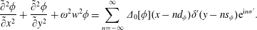 $$\begin{eqnarray}\displaystyle \frac{\tilde{\unicode[STIX]{x2202}}^{2}\unicode[STIX]{x1D719}}{\tilde{\unicode[STIX]{x2202}}x^{2}}+\frac{\tilde{\unicode[STIX]{x2202}}^{2}\unicode[STIX]{x1D719}}{\tilde{\unicode[STIX]{x2202}}y^{2}}+\unicode[STIX]{x1D714}^{2}w^{2}\unicode[STIX]{x1D719}=\mathop{\sum }_{n=-\infty }^{\infty }\unicode[STIX]{x1D6E5}_{0}[\unicode[STIX]{x1D719}](x-nd)\unicode[STIX]{x1D6FF}^{\prime }(y-ns)\text{e}^{\text{i}n\unicode[STIX]{x1D70E}^{\prime }}. & & \displaystyle\end{eqnarray}$$
We define the Fourier integral transform and its inverse as
 $$\begin{eqnarray}\displaystyle & \displaystyle F(\unicode[STIX]{x1D6FE},\unicode[STIX]{x1D702})=\frac{1}{(2\unicode[STIX]{x03C0})^{2}}\int _{-\infty }^{\infty }\int _{-\infty }^{\infty }f(x,y)\text{e}^{\text{i}\unicode[STIX]{x1D6FE}x+\text{i}\unicode[STIX]{x1D702}y}\,\text{d}x\,\text{d}y, & \displaystyle \nonumber\\ \displaystyle & \displaystyle f(x,y)=\int _{-\infty }^{\infty }\int _{-\infty }^{\infty }F(\unicode[STIX]{x1D6FE},\unicode[STIX]{x1D702})\text{e}^{-\text{i}\unicode[STIX]{x1D6FE}x-\text{i}\unicode[STIX]{x1D702}y}\,\text{d}\unicode[STIX]{x1D6FE}\,\text{d}\unicode[STIX]{x1D702}. & \displaystyle \nonumber\end{eqnarray}$$
Applying the transform to the left-hand side of (3.4) yields
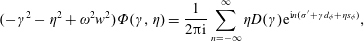 $$\begin{eqnarray}\displaystyle (-\unicode[STIX]{x1D6FE}^{2}-\unicode[STIX]{x1D702}^{2}+\unicode[STIX]{x1D714}^{2}w^{2})\unicode[STIX]{x1D6F7}(\unicode[STIX]{x1D6FE},\unicode[STIX]{x1D702})=\frac{1}{2\unicode[STIX]{x03C0}\text{i}}\mathop{\sum }_{n=-\infty }^{\infty }\unicode[STIX]{x1D702}D(\unicode[STIX]{x1D6FE})\text{e}^{\text{i}n(\unicode[STIX]{x1D70E}^{\prime }+\unicode[STIX]{x1D6FE}d+\unicode[STIX]{x1D702}s)}, & & \displaystyle\end{eqnarray}$$
 where  $\unicode[STIX]{x1D6F7}$ is the Fourier transform of $\unicode[STIX]{x1D719}$. The problem is now to find $D(\unicode[STIX]{x1D6FE})$ which represents the Fourier transform of the jump in acoustic potential either side of the blade and wake
 $$\begin{eqnarray}\displaystyle D(\unicode[STIX]{x1D6FE})=\frac{1}{2\unicode[STIX]{x03C0}}\int _{0}^{\infty }\unicode[STIX]{x1D6E5}_{0}[\unicode[STIX]{x1D719}](x)\text{e}^{\text{i}\unicode[STIX]{x1D6FE}x}\,\text{d}x. & & \displaystyle \nonumber\end{eqnarray}$$
 We invert the Fourier transform to obtain an expression for the acoustic potential in terms of  $D$
$D$
 $$\begin{eqnarray}\displaystyle \unicode[STIX]{x1D719}(x,y)=\frac{1}{2\unicode[STIX]{x03C0}\text{i}}\int _{-\infty }^{\infty }\int _{-\infty }^{\infty }\frac{\text{e}^{-\text{i}\unicode[STIX]{x1D6FE}x-\text{i}\unicode[STIX]{x1D702}y}}{\unicode[STIX]{x1D714}^{2}w^{2}-\unicode[STIX]{x1D702}^{2}-\unicode[STIX]{x1D6FE}^{2}}\cdot \mathop{\sum }_{n=-\infty }^{\infty }\unicode[STIX]{x1D702}D(\unicode[STIX]{x1D6FE})\text{e}^{\text{i}n(\unicode[STIX]{x1D70E}^{\prime }+\unicode[STIX]{x1D6FE}d+\unicode[STIX]{x1D702}s)}\,\text{d}\unicode[STIX]{x1D6FE}\,\text{d}\unicode[STIX]{x1D702}. & & \displaystyle\end{eqnarray}$$
 The  $\unicode[STIX]{x1D702}$ integral may be performed by closing the contour of integration in an appropriate upper or lower half-plane to obtain
 $$\begin{eqnarray}\displaystyle \unicode[STIX]{x1D719}(x,y)=-\frac{1}{2}\int _{-\infty }^{\infty }\mathop{\sum }_{n=-\infty }^{\infty }D(\unicode[STIX]{x1D6FE})\text{sgn}(ns-y)\text{e}^{\text{i}n(\unicode[STIX]{x1D70E}^{\prime }+\unicode[STIX]{x1D6FE}d)+\text{i}\unicode[STIX]{x1D701}|ns-y|}\text{e}^{-\text{i}\unicode[STIX]{x1D6FE}x}\,\text{d}\unicode[STIX]{x1D6FE}, & & \displaystyle\end{eqnarray}$$
 where  $\unicode[STIX]{x1D701}=\sqrt{\unicode[STIX]{x1D714}^{2}w^{2}-\unicode[STIX]{x1D6FE}^{2}}$. The branch cut is defined so that $\text{Im}[\unicode[STIX]{x1D701}]>0$ when $\unicode[STIX]{x1D6FE}$ is in a strip for the Wiener–Hopf method.
To obtain an equation for the unknown  $D$ we must apply the relevant boundary conditions. We first differentiate (3.7) with respect to $y$ and consider the limits $y\rightarrow 0^{\pm }$. Summing the contributions from each of these limits yields the integral equation
 $$\begin{eqnarray}\displaystyle \unicode[STIX]{x1D6F4}_{0}\left[\frac{\unicode[STIX]{x2202}\unicode[STIX]{x1D719}}{\unicode[STIX]{x2202}y}\right](x)=4\unicode[STIX]{x03C0}\int _{-\infty }^{\infty }D(\unicode[STIX]{x1D6FE})j(\unicode[STIX]{x1D6FE})\text{e}^{-\text{i}\unicode[STIX]{x1D6FE}x}\,\text{d}\unicode[STIX]{x1D6FE}, & & \displaystyle\end{eqnarray}$$
where
 $$\begin{eqnarray}\displaystyle j(\unicode[STIX]{x1D6FE})=\frac{\text{i}\unicode[STIX]{x1D701}}{4\unicode[STIX]{x03C0}}\mathop{\sum }_{n\in \mathbb{Z}}\text{e}^{\text{i}n(\unicode[STIX]{x1D70E}^{\prime }+\unicode[STIX]{x1D6FE}d)+\text{i}\unicode[STIX]{x1D701}|ns|}=\frac{\unicode[STIX]{x1D701}}{4\unicode[STIX]{x03C0}}\cdot \frac{\sin (\unicode[STIX]{x1D701}s)}{\cos (\unicode[STIX]{x1D701}s)-\cos (\unicode[STIX]{x1D6FE}d+\unicode[STIX]{x1D70E}^{\prime })}. & & \displaystyle\end{eqnarray}$$
 We now solve (3.8) subject to the remaining boundary conditions applied on  $y=0$
$y=0$
 $$\begin{eqnarray}\displaystyle \unicode[STIX]{x1D6E5}_{0}[\unicode[STIX]{x1D719}](x)=0,\quad x<0, & & \displaystyle\end{eqnarray}$$
 $$\begin{eqnarray}\displaystyle \unicode[STIX]{x1D6F4}_{0}\left[\frac{\unicode[STIX]{x2202}\unicode[STIX]{x1D719}}{\unicode[STIX]{x2202}y}\right](x) & = & \displaystyle \unicode[STIX]{x1D707}_{0}\unicode[STIX]{x1D6E5}_{0}[\unicode[STIX]{x1D719}](x)+\unicode[STIX]{x1D707}_{1}\unicode[STIX]{x1D6E5}_{0}[\unicode[STIX]{x1D719}_{x}](x)+\unicode[STIX]{x1D707}_{2}\unicode[STIX]{x1D6E5}_{0}[\unicode[STIX]{x1D719}_{x,x}](x)\nonumber\\ \displaystyle & & \displaystyle -\,2w_{0}\exp [\text{i}(k_{x}/\unicode[STIX]{x1D6FD}^{2})x],\quad 0<x<2,\end{eqnarray}$$
 $$\begin{eqnarray}\displaystyle \unicode[STIX]{x1D6E5}_{0}[\unicode[STIX]{x1D719}](x)=2\unicode[STIX]{x03C0}\text{i}P\exp [\text{i}(\unicode[STIX]{x1D714}/\unicode[STIX]{x1D6FD}^{2})x],\quad x>2. & & \displaystyle\end{eqnarray}$$
 The system ((3.8), (3.10a), (3.10b), (3.10c)) represents an integral equation subject to mixed value boundary conditions. We solve this system via the Wiener–Hopf method as detailed in appendix A. The solution for  $D$ is given by
 $$\begin{eqnarray}\displaystyle D(\unicode[STIX]{x1D6FE}) & = & \displaystyle \frac{w_{0}}{(2\unicode[STIX]{x03C0})^{2}\text{i}(\unicode[STIX]{x1D6FE}+k_{x}/\unicode[STIX]{x1D6FD}^{2})K_{-}(-k_{x}/\unicode[STIX]{x1D6FD}^{2})K_{+}(\unicode[STIX]{x1D6FE})}\nonumber\\ \displaystyle & & \displaystyle +\,\frac{w_{0}(\unicode[STIX]{x1D714}-k_{x})\text{e}^{2\text{i}(\unicode[STIX]{x1D6FE}+k_{x}/\unicode[STIX]{x1D6FD}^{2})}}{(2\unicode[STIX]{x03C0}\unicode[STIX]{x1D6FD})^{2}\text{i}(\unicode[STIX]{x1D6FE}+k_{x}/\unicode[STIX]{x1D6FD}^{2})(\unicode[STIX]{x1D6FE}+\unicode[STIX]{x1D714}/\unicode[STIX]{x1D6FD}^{2})K_{+}(-k_{x}/\unicode[STIX]{x1D6FD}^{2})K_{-}(\unicode[STIX]{x1D6FE})}\nonumber\\ \displaystyle & & \displaystyle -\,\mathop{\sum }_{n=0}^{\infty }\frac{({\mathcal{A}}_{n}+{\mathcal{C}}_{n})\text{e}^{2\text{i}(\unicode[STIX]{x1D6FE}-\unicode[STIX]{x1D703}_{n}^{-})}}{\text{i}(\unicode[STIX]{x1D6FE}+\unicode[STIX]{x1D714}/\unicode[STIX]{x1D6FD}^{2})(\unicode[STIX]{x1D6FE}-\unicode[STIX]{x1D703}_{n}^{-})}\cdot \frac{K_{-}(\unicode[STIX]{x1D703}_{n}^{-})}{K_{-}(\unicode[STIX]{x1D6FE})}-\mathop{\sum }_{n=0}^{\infty }\frac{{\mathcal{B}}_{n}}{\unicode[STIX]{x1D6FE}-\unicode[STIX]{x1D703}_{n}^{+}}\cdot \frac{K_{+}(\unicode[STIX]{x1D703}_{n}^{+})}{K_{+}(\unicode[STIX]{x1D6FE})},\end{eqnarray}$$
 where all new variables are defined in appendix A. Note that the solution is identical to that for the type 0 cascade (Glegg Reference Glegg1999), except the original Wiener–Hopf kernel  $j$ is now replaced with the modified kernel $K$. This original kernel is recovered when $\unicode[STIX]{x1D707}_{1}=\unicode[STIX]{x1D707}_{2}=\unicode[STIX]{x1D707}_{3}=0$ and the solution reduces to that derived by Glegg (Reference Glegg1999).
3.1 Inversion of Fourier transform
We now invert the Fourier transform of the previous section to obtain the acoustic potential function. Since  $D$ is now known, the Fourier inversion integral in (3.7) can now be computed. Similarly to the analysis in Posson et al. (Reference Posson, Roger and Moreau2010), the inversion is performed by splitting the physical domain into five regions as illustrated in figure 5. Each solution is simply a sum of exponential functions. The details can be found in appendix C and the final results are stated below. All undefined functions are defined in appendices A and C.
Diagram indicating the different regions in the  $(x,y)$-plane which require different areas of contour integration in the Fourier inversion.

3.1.1 Upstream region (I)
In the upstream region,
 $$\begin{eqnarray}\displaystyle \unicode[STIX]{x1D719}(x,y)=2\unicode[STIX]{x03C0}\text{i}\mathop{\sum }_{m=-\infty }^{\infty }D^{(1,3)}(\unicode[STIX]{x1D706}_{m}^{+})A^{r}(x,y;\unicode[STIX]{x1D706}_{m}^{+}). & & \displaystyle\end{eqnarray}$$
3.1.2 Inter-blade upstream region (II)
In the inter-blade upstream region,
 $$\begin{eqnarray}\displaystyle \unicode[STIX]{x1D719}(x,y) & = & \displaystyle -2\unicode[STIX]{x03C0}\mathop{\sum }_{n=0}^{\infty }\frac{{\mathcal{A}}_{n}+{\mathcal{C}}_{n}}{\unicode[STIX]{x1D703}_{n}^{-}+\unicode[STIX]{x1D714}/\unicode[STIX]{x1D6FD}^{2}}A_{d}(x,y;\unicode[STIX]{x1D703}_{n}^{-})+2\unicode[STIX]{x03C0}\text{i}\mathop{\sum }_{n=0}^{\infty }{\mathcal{B}}_{n}A_{d}(x,y;\unicode[STIX]{x1D703}_{n}^{+})\nonumber\\ \displaystyle & & \displaystyle -\,\frac{A_{d}(x,y;-k_{x}/\unicode[STIX]{x1D6FD}^{2})}{K(-k_{x}/\unicode[STIX]{x1D6FD}^{2})}\,\frac{w_{0}}{2\unicode[STIX]{x03C0}}+2\unicode[STIX]{x03C0}\text{i}\mathop{\sum }_{m=-\infty }^{\infty }D^{(1,3)}(\unicode[STIX]{x1D706}_{m}^{+})A_{u}^{r}(x,y;\unicode[STIX]{x1D706}_{m}^{+}).\nonumber\end{eqnarray}$$
3.1.3 Inter-blade inner region (III)
In the inter-blade inner region,
 $$\begin{eqnarray}\displaystyle \unicode[STIX]{x1D719}(x,y) & = & \displaystyle -2\unicode[STIX]{x03C0}\mathop{\sum }_{n=0}^{\infty }\frac{{\mathcal{A}}_{n}+{\mathcal{C}}_{n}}{\unicode[STIX]{x1D703}_{n}^{-}+\unicode[STIX]{x1D714}/\unicode[STIX]{x1D6FD}^{2}}A(x,y;\unicode[STIX]{x1D703}_{n}^{-})+2\unicode[STIX]{x03C0}\text{i}\mathop{\sum }_{n=0}^{\infty }{\mathcal{B}}_{n}A(\unicode[STIX]{x1D703}_{n}^{+},x,y)\nonumber\\ \displaystyle & & \displaystyle -\,\frac{A(x,y;-k_{x}/\unicode[STIX]{x1D6FD}^{2})}{K(-k_{x}/\unicode[STIX]{x1D6FD}^{2})}\,\frac{w_{0}}{2\unicode[STIX]{x03C0}}.\nonumber\end{eqnarray}$$
3.1.4 Inter-blade downstream region (IV)
In the inter-blade downstream region,
 $$\begin{eqnarray}\displaystyle \unicode[STIX]{x1D719}(x,y) & = & \displaystyle -2\unicode[STIX]{x03C0}\mathop{\sum }_{n=0}^{\infty }\frac{{\mathcal{A}}_{n}+{\mathcal{C}}_{n}}{\unicode[STIX]{x1D703}_{n}^{-}+\unicode[STIX]{x1D714}/\unicode[STIX]{x1D6FD}^{2}}A_{u}(x,y;\unicode[STIX]{x1D703}_{n}^{-})+2\unicode[STIX]{x03C0}\text{i}\mathop{\sum }_{n=0}^{\infty }{\mathcal{B}}_{n}A_{u}(x,y;\unicode[STIX]{x1D703}_{n}^{+})\nonumber\\ \displaystyle & & \displaystyle -\,\frac{A_{u}(x,y;-k_{x}/\unicode[STIX]{x1D6FD}^{2})}{K(-k_{x}/\unicode[STIX]{x1D6FD}^{2})}\,\frac{w_{0}}{2\unicode[STIX]{x03C0}}\nonumber\\ \displaystyle & & \displaystyle -\,2\unicode[STIX]{x03C0}\text{i}\mathop{\sum }_{m=-\infty }^{\infty }D^{(2,4)}(\unicode[STIX]{x1D706}_{m}^{-})A_{d}^{r}(x,y;\unicode[STIX]{x1D706}_{m}^{-})+2\unicode[STIX]{x03C0}\text{i}PA_{d}(x,y;-\unicode[STIX]{x1D714}/\unicode[STIX]{x1D6FD}^{2}).\nonumber\end{eqnarray}$$
3.1.5 Downstream region (V)
In the downstream region,
 $$\begin{eqnarray}\displaystyle \unicode[STIX]{x1D719}(x,y)=-2\unicode[STIX]{x03C0}\text{i}\mathop{\sum }_{m=-\infty }^{\infty }D^{(2,4)}(\unicode[STIX]{x1D706}_{m}^{-})A^{r}(x,y;\unicode[STIX]{x1D706}_{m}^{-})+2\unicode[STIX]{x03C0}\text{i}PA(x,y;-\unicode[STIX]{x1D714}/\unicode[STIX]{x1D6FD}^{2}). & & \displaystyle\end{eqnarray}$$
4 Results
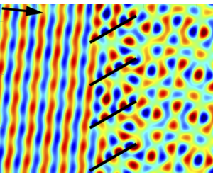
We now use the analytic solution derived in § 3.1 to explore the aeroacoustic performance of a blade row with modified boundary conditions. In particular, we focus on the role of porosity due to its potential to attenuate sound, as seen previously in Jaworski & Peake (Reference Jaworski and Peake2013) for trailing-edge scattering. Porous blades in flow are represented by the case II boundary condition in the present nomenclature. The results in the present research also show significant sound reductions for modest changes in porosity. We argue that this is attributed to the strong effect of porosity on the duct modes and unsteady loading: in cascade configurations, the blade loading changes the upstream and downstream flows and therefore influences the intensity of the scattered sound.
Although the solution is formally analytic, there are two steps that must be handled numerically. First, the linear system comprised of (A 33) and (A 36) must be solved. Second, the zeros of the meromorphic kernel  $K$ must be located in the complex plane. For large zeros ( $|\unicode[STIX]{x1D703}_{j}|\gg 1$), the asymptotic approximations in § B.2 can reliably be used as initial guesses for an iterative Newton scheme. For other zeros ( $|\unicode[STIX]{x1D703}_{j}|\sim 1$), we use a modified version of the Delves & Lyness (Reference Delves and Lyness1967) algorithm to ensure that all the zeros in a prescribed region are found. The relevant integrations are computed using the trapezoidal rule, which converges geometrically for integrals of meromorphic functions over ellipses (Trefethen & Weideman Reference Trefethen and Weideman2014). This rapid numerical implementation allows all relevant aeroacoustic quantities to be evaluated in a fraction of a second using the code publicised in the introduction.
4.1 Validation
We first present a comparison to three previous solutions for cascades of impermeable and rigid blades in figure 6. First, we compare our results to a solution exploiting the Wiener–Hopf method (Posson et al. Reference Posson, Roger and Moreau2010). Second, we compare to a quasi-numerical a mode-matching technique (Bouley et al. Reference Bouley, François, Roger, Posson and Moreau2017), and third, we compare to a fully numerical method (Hall Reference Hall1997). The solutions show excellent agreement – in fact our case 0 solution is mathematically equivalent to the of Posson et al. (Reference Posson, Roger and Moreau2010). It is worth noting at this point that our solution satisfies the Kutta condition, as indicated by the pressure jump vanishing at the trailing edge.
Comparisons of surface pressure jump for flat plates for case 0 boundary conditions and geometries defined in table 2. The real and imaginary parts (blue and red respectively) of the pressure jump are compared to three alternative solutions: a Wiener–Hopf method (Posson et al. Reference Posson, Roger and Moreau2010), a mode-matching technique (Bouley et al. Reference Bouley, François, Roger, Posson and Moreau2017) and a numerical method (Hall Reference Hall1997).
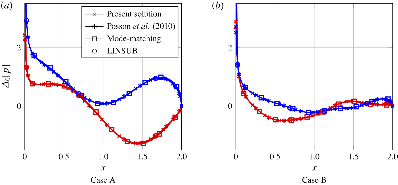
4.2 Duct mode analysis
The cascade may be divided into five regions as illustrated in figure 5. Since we only consider the case where the blades are overlapping, the inter-blade inner region (called region III) is bounded by adjacent blades and therefore may be viewed as a duct. The solution in the duct is matched to the upstream and downstream regions by virtue of the inter-blade upstream region (II) and the inter-blade downstream region (IV). The duct region is therefore essential in establishing the relationship between the upstream and downstream regions, and controls the unsteady lift and sound power output. We now explore the behaviour of the solution in the duct in order to understand the effects of blade porosity.
The acoustic potential in the duct may be expanded into a sum of exponential functions whose modes are the ‘duct modes’ (Glegg & Devenport Reference Glegg and Devenport2017). For type 0 blades, the duct has rigid, impermeable walls and the modes are given by the standard formula
 $$\begin{eqnarray}\displaystyle \hat{\unicode[STIX]{x1D703}}_{n}^{\pm }=\pm \sqrt{\unicode[STIX]{x1D714}^{2}w^{2}-\left(\frac{n\unicode[STIX]{x03C0}}{s}\right)^{2}}, & & \displaystyle\end{eqnarray}$$
 where we have used  $\hat{\cdot }$ to indicate that this solution is valid for case 0 ( $C_{II}=0$). Conversely, there is no simple expression for the duct modes when the blades are porous; for porosity constant $C_{II}$ the duct modes satisfy the transcendental equation
 $$\begin{eqnarray}\displaystyle \unicode[STIX]{x1D701}(\unicode[STIX]{x1D703}_{n}^{\pm })\sin (s\unicode[STIX]{x1D701}(\unicode[STIX]{x1D703}_{n}^{\pm }))=\text{i}C_{II}(\unicode[STIX]{x1D714}/\unicode[STIX]{x1D6FD}^{2}+\unicode[STIX]{x1D703}_{n}^{\pm })(\cos (s\unicode[STIX]{x1D701}(\unicode[STIX]{x1D703}_{n}^{\pm }))-\cos (d\unicode[STIX]{x1D703}_{n}^{\pm }+\unicode[STIX]{x1D70E}^{\prime })). & & \displaystyle\end{eqnarray}$$
 The solutions for large  $\unicode[STIX]{x1D703}_{n}^{\pm }$ are available via the asymptotic analysis presented in § B.2, but otherwise the solutions must generally be found with a numerical root finding algorithm (Delves & Lyness Reference Delves and Lyness1967).
It is straightforward to see from (4.1) that the  $n$th case 0 duct mode is pure imaginary when $\unicode[STIX]{x1D714}w<n\unicode[STIX]{x03C0}/s$ and pure real when $\unicode[STIX]{x1D714}w>n\unicode[STIX]{x03C0}/s$. These conditions correspond to the duct mode being cut-off or cut-on. However, inspection of (4.2) reveals that for an arbitrary finite porosity constant $C_{II}$ (but not pure imaginary), it is impossible for the duct modes to be cut-on. This is readily seen by noting that there are no real solutions to (4.2). If a real root did exist, then the left hand side would be pure real. However, in that case the right hand side has a non-zero imaginary part, and we have a contradiction. Consequently, for any non-imaginary porosity coefficients, the duct modes are always complex and never pure real. Accordingly, blade porosity effects a reduction in the magnitude of the pressure field in the inter-blade inner region which, when matched to the upstream and downstream regions, results in a reduction in the far-field scattered sound.
The dependence of the duct modes on blade porosity is illustrated in figure 7 for two frequencies. There are no acoustic modes cut-on in figure 7(a), whereas there are two acoustic modes cut-on in figure 7(b). Modes located in the upper or lower half plane (denoted by  ${\mathcal{L}}^{\pm }$) are propagating in the upstream and downstream directions respectively. We consider a range of arguments for the porosity coefficient to represent a phase difference between the pressure jump and normal velocity, which is permitted due to the presence of the background flow (Howe et al. Reference Howe, Scott and Sipcic1996). Evidently, the relationship between the duct modes is highly complex, although some general trends may be observed. In compliance with the argument in the preceding paragraph, all values of porosity (except pure imaginary) perturb the cut-on duct modes away from the real line. For zero porosity, the duct modes are located at the rigid duct modes, $\hat{\unicode[STIX]{x1D703}}_{n}^{\pm }$. As the porosity is increased, the duct modes follow a path that generally ends at either the convected mode ( $-\unicode[STIX]{x1D714}/\unicode[STIX]{x1D6FD}^{2}$) or an acoustic mode ( $\unicode[STIX]{x1D706}_{n}^{\pm }$).
The trajectories of the duct modes for a range of (complex) porosity coefficients for case C described in table 2, with  $k_{x}=4$. Along each line, the phase of $C_{II}$ is held constant while its magnitude is increased from $0$ to $\infty$. For example, the duct modes corresponding to real and positive values of $C_{II}$ are illustrated in red. The duct modes for case 0 blades (i.e. $C_{II}=0$) are denoted by ●, the acoustic modes, $\unicode[STIX]{x1D706}_{m}$, are labelled denoted by ▪ and the convected mode ( $-\unicode[STIX]{x1D714}/\unicode[STIX]{x1D6FD}^{2}$) is denoted by ▴. Accordingly, each trajectory begins at a ● and ends at either a ▪ or a ▴. The upper half-plane ${\mathcal{L}}^{+}$ is shaded in red and the lower half-plane ${\mathcal{L}}^{-}$ is shaded in blue.
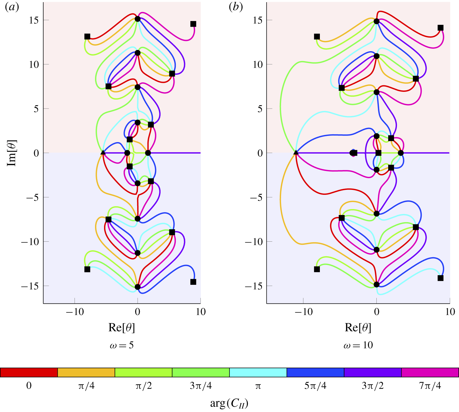
It is instructive to inspect the asymptotic forms of the duct modes for small and large values of porosity. For small Rayleigh conductivity ( $|C_{II}|\ll 1$, $\arg (C_{II})\neq \pm \unicode[STIX]{x03C0}/2$), the roots are a small perturbation away from the case 0 duct modes
 $$\begin{eqnarray}\displaystyle \unicode[STIX]{x1D703}_{n}^{\pm }=\hat{\unicode[STIX]{x1D703}}_{n}^{\pm }-C_{II}\frac{\text{i}(\unicode[STIX]{x1D714}/\unicode[STIX]{x1D6FD}^{2}+\hat{\unicode[STIX]{x1D703}}_{n}^{\pm })}{s(1+\unicode[STIX]{x1D6FF}_{0,n})\hat{\unicode[STIX]{x1D703}}_{n}^{\pm }}(1-(-1)^{n}\cos (d\hat{\unicode[STIX]{x1D703}}_{n}^{\pm }+\unicode[STIX]{x1D70E}^{\prime }))+o(C_{II}). & & \displaystyle\end{eqnarray}$$
 Conversely, for large Rayleigh conductivity ( $|C_{II}|\gg 1$, $\arg (C_{II})\neq \pm \unicode[STIX]{x03C0}/2$), the duct modes are a small perturbation away from either the hydrodynamic mode or the acoustic modes:
 $$\begin{eqnarray}\displaystyle & \displaystyle \unicode[STIX]{x1D703}_{0}=-\unicode[STIX]{x1D714}/\unicode[STIX]{x1D6FD}^{2}-\frac{1}{C_{II}}\,\frac{\text{i}\unicode[STIX]{x1D701}(-\unicode[STIX]{x1D714}/\unicode[STIX]{x1D6FD}^{2})\sin (s\unicode[STIX]{x1D701}(-\unicode[STIX]{x1D714}/\unicode[STIX]{x1D6FD}^{2}))}{\cos (s\unicode[STIX]{x1D701}(-\unicode[STIX]{x1D714}/\unicode[STIX]{x1D6FD}^{2}))-\cos (\unicode[STIX]{x1D70E}^{\prime }-d\unicode[STIX]{x1D714}/\unicode[STIX]{x1D6FD}^{2})}+o(C_{II}^{-1}), & \displaystyle\end{eqnarray}$$
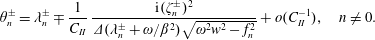 $$\begin{eqnarray}\displaystyle & \displaystyle \unicode[STIX]{x1D703}_{n}^{\pm }=\unicode[STIX]{x1D706}_{n}^{\pm }\mp \frac{1}{C_{II}}\,\frac{\text{i}(\unicode[STIX]{x1D701}_{n}^{\pm })^{2}}{\unicode[STIX]{x1D6E5}(\unicode[STIX]{x1D706}_{n}^{\pm }+\unicode[STIX]{x1D714}/\unicode[STIX]{x1D6FD}^{2})\sqrt{\unicode[STIX]{x1D714}^{2}w^{2}-f_{n}^{2}}}+o(C_{II}^{-1}),\quad n\neq 0. & \displaystyle\end{eqnarray}$$ $C_{II}$ is increased to 1, which is suggests that large aeroacoustic gains can be made for modest porosity coefficients. This assertion is explored further in the following sections.
The imaginary parts of the duct modes as a function of (real) porosity coefficient  $C_{II}$. The asymptotic approximations for small porosity coefficients (4.3) as illustrated by the dashed blue lines and the asymptotic approximations for large porosity coefficients ((4.4a), (4.4b)) are denoted by the dashed red lines. The cascade parameters are defined in case C in table 2 with $\unicode[STIX]{x1D714}=5$ and $k_{x}=4$.
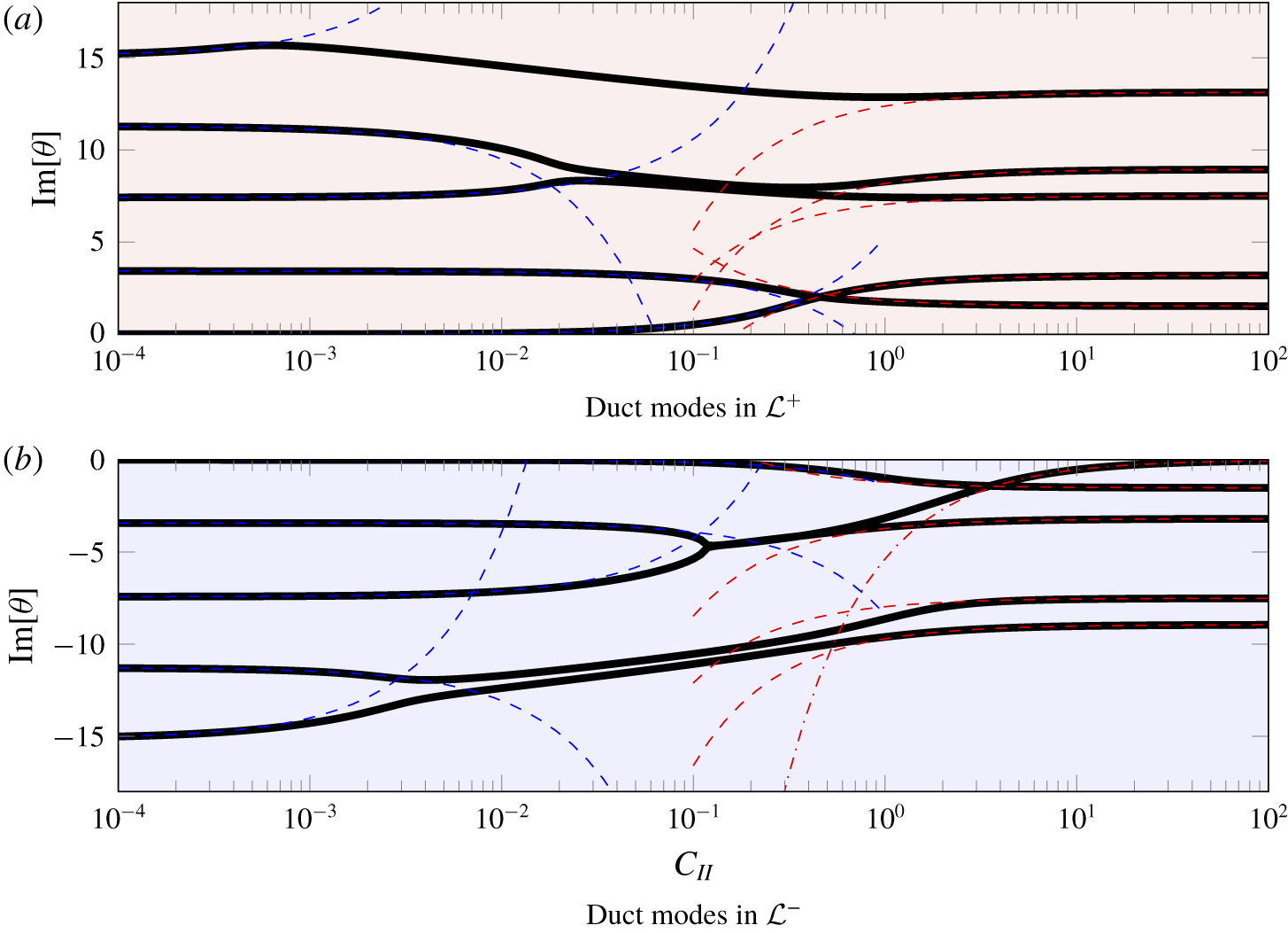
The trajectories of a pair of duct modes as the frequency is increased for a range of porosity constants. The duct modes for  $\unicode[STIX]{x1D714}=0$ are denoted by ●. The complex trajectories are plotted in (a), and the imaginary part of the modes in the upper and lower half planes are plotted in (b,c) respectively. The colours correspond to different porosity parameters with black representing rigid and impermeable blades. The upper half-plane ${\mathcal{L}}^{+}$ is shaded in red and the lower half-plane ${\mathcal{L}}^{-}$ is shaded in blue. The relevant parameters correspond to case D in table 2 with $k_{x}=2$.
Further insight may be gained by examining the duct modes as a function of frequency for fixed porosity values. Figure 9 illustrates the duct modes for four porosity coefficients at a range of frequencies. For each porosity value, the imaginary part of the mode decreases as the frequency is increased. However, in contrast for case 0 blades, the imaginary part never vanishes for non-zero porosity values. In some cases (in  ${\mathcal{L}}^{+}$), the imaginary part of the duct modes undergoes a slight increase before decreasing towards the real axis. The role of porosity is particularly important for small to moderate frequencies. As the frequency is increased, the difference between the modes reduces.
We now consider the effect of porosity on sound generation and sound transmission.
4.3 Sound generation
Sound generation is caused when a pressure-free gust interacts with the blade row, resulting in the production of pressure waves. The incident perturbation can also be described as a ‘vorticity wave’ and is convected with the background flow so that  $k_{x}=\unicode[STIX]{x1D714}$. In order to enable comparison against prior works, we consider cases analysed by Glegg (Reference Glegg1999) and Posson et al. (Reference Posson, Roger and Moreau2010) as defined in table 2. We consider cases where $C_{II}<0$ so that the imaginary part of the Rayleigh conductivity is negative and the pores dissipate energy.
Summary of parameters used in results section. All other parameters are taken to be zero, unless otherwise stated.
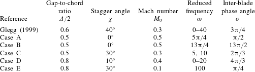
4.3.1 Unsteady lift
During the solution to the Wiener–Hopf problem associated with the scattering by a blade row with complex boundaries, we observed that the major difference with the rigid, impermeable case is that the duct modes are modified by the boundary conditions. Consequently, we expect complex boundary conditions to have a significant effect on the unsteady loading of the blades. In this section we test that hypothesis.
The analytic expression for  $D$ (3.11) enables the swift calculation of the unsteady loading on the blades. The unsteady loading is defined as the integral of the unsteady pressure over the blade surface
 $$\begin{eqnarray}\displaystyle C_{L}=\frac{1}{2\unicode[STIX]{x03C0}w_{0}}\int _{0}^{2}\unicode[STIX]{x1D6E5}_{0}[p](x)\,\text{d}x. & & \displaystyle\end{eqnarray}$$
Integration by parts and application of the boundary conditions (3.10a) and (3.10c) yields the identity
 $$\begin{eqnarray}\displaystyle D(-\unicode[STIX]{x1D714}M_{0}^{2}/\unicode[STIX]{x1D6FD}^{2}) & = & \displaystyle \frac{1}{2\unicode[STIX]{x03C0}}\int _{-\infty }^{\infty }\unicode[STIX]{x1D6E5}_{0}[\unicode[STIX]{x1D719}](x)\text{e}^{-\text{i}\unicode[STIX]{x1D714}(M_{0}/\unicode[STIX]{x1D6FD})^{2}x}\,\text{d}x\nonumber\\ \displaystyle & = & \displaystyle -\frac{1}{\text{i}\unicode[STIX]{x1D714}2\unicode[STIX]{x03C0}}\int _{0}^{2}\frac{\unicode[STIX]{x2202}}{\unicode[STIX]{x2202}x}(\unicode[STIX]{x1D6E5}_{0}[\unicode[STIX]{x1D719}](x)\text{e}^{-\text{i}(\unicode[STIX]{x1D714}/\unicode[STIX]{x1D6FD}^{2})x})\text{e}^{\text{i}\unicode[STIX]{x1D714}x}\,\text{d}x.\nonumber\end{eqnarray}$$
Consequently, the normalised unsteady lift (4.5) may be written as
 $$\begin{eqnarray}\displaystyle C_{L}=\frac{\text{i}\unicode[STIX]{x1D714}}{w_{0}}D(-\unicode[STIX]{x1D714}M^{2}/\unicode[STIX]{x1D6FD}^{2}). & & \displaystyle \nonumber\end{eqnarray}$$
Unsteady lift for a range of frequencies and porosities. The aerodynamic and aeroacoustic parameters are defined in table 2 and correspond to those in figure 3 of Glegg (Reference Glegg1999). The colours correspond to different porosity parameters with black representing rigid and impermeable blades.
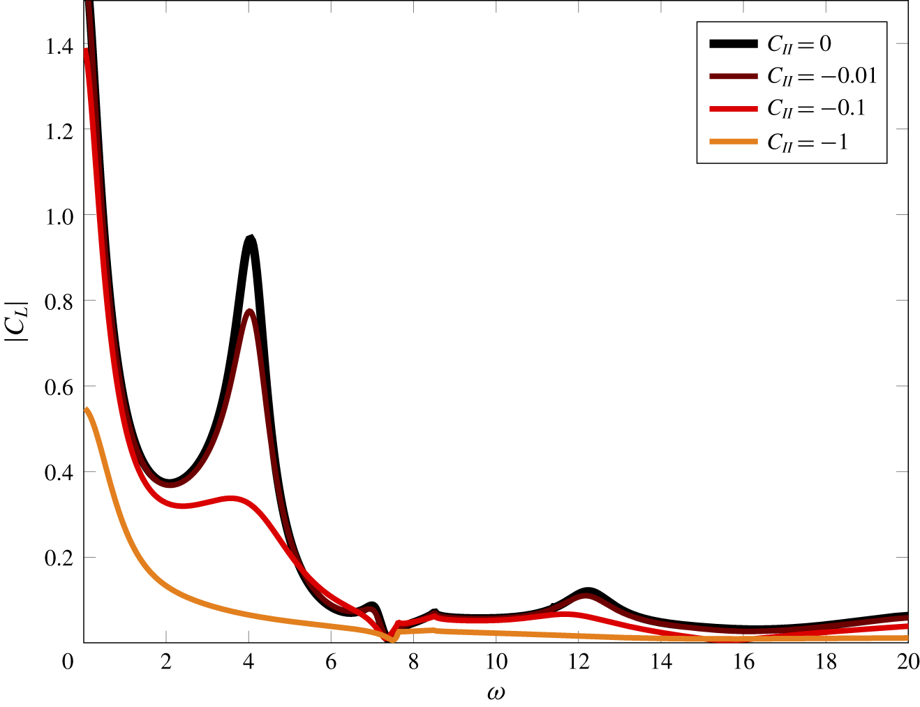
Modal downstream sound power output for a cascade of porous blades at a range of frequencies for (a) the first mode ( $m=0$) and (b) the second mode ( $m=1$). The aerodynamic and aeroacoustic parameters are defined in table 2 and correspond to those in figure 9 of Glegg (Reference Glegg1999). The colours correspond to different porosity parameters with black representing rigid and impermeable blades.
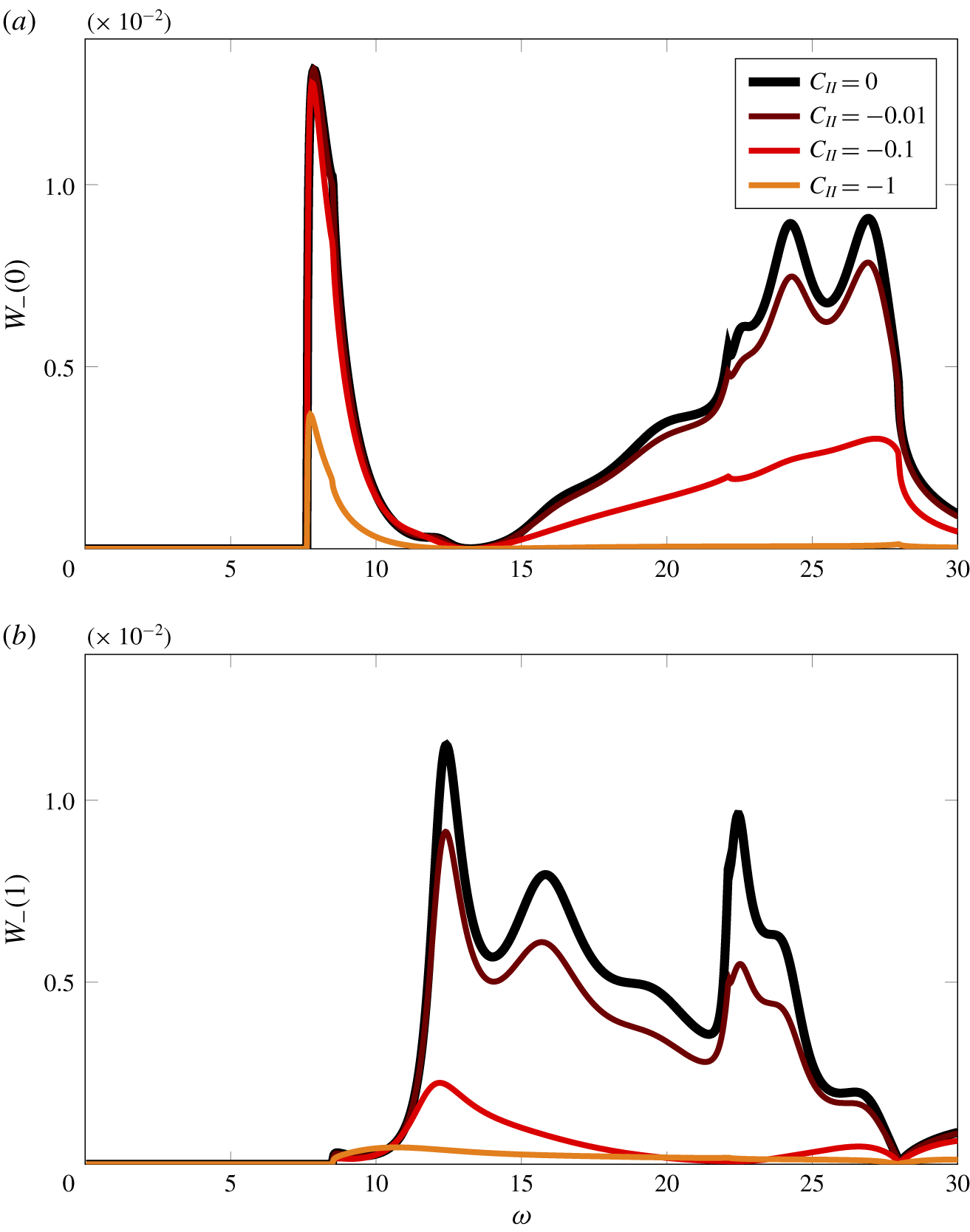
The modified boundary conditions have a strong effect on the unsteady loading, as illustrated in figure 10. The unsteady loading for a case 0 cascade is compared against the loading for a range of porosity parameters, which correspond to the  $C_{II}$ values. The results indicate that the effect of the modified boundary conditions is to shift the locations of the duct modes, as indicated by the shifts in the local maximum around $\unicode[STIX]{x1D714}\approx 12$, which has previously been identified with the cut-on frequency of the duct mode (Glegg Reference Glegg1999). As $C_{II}$ decreases, the pressure jump across the blade must decrease in accordance with the Rayleigh conductivity (2.15), thus ensuring that the seepage velocity through the blade is proportional to the pressure jump across the blade. This is observed in figure 10, where the effects of increasing the porosity result in an almost uniform reduction in the unsteady lift.
The impact of porosity on unsteady lift appears most pronounced when the frequency is low, which is fortuitous since the homogenised boundary condition (2.15) is most valid in the low-frequency regime. In particular, the range  $0<\unicode[STIX]{x1D714}<7.62$ shows the largest reduction in lift, and the peak around $\unicode[STIX]{x1D714}\approx 4$ is greatly attenuated. After the acoustic mode is cut-on at $\unicode[STIX]{x1D714}\approx 7.62$, the reductions in lift are generally smaller, but this is possibly because the lift on the case 0 cascade is also reduced; as a percentage, the reductions still appear significant.
4.3.2 Sound power output
Analytic expressions for the sound power output are available by a similar method to Glegg (Reference Glegg1999). The modal upstream or downstream sound power output for the  $m$th mode is given by
 $$\begin{eqnarray}\displaystyle W_{\pm }(m)=\frac{\unicode[STIX]{x1D714}\unicode[STIX]{x03C0}^{2}}{\unicode[STIX]{x1D6E5}}\text{Re}\left[\frac{|\unicode[STIX]{x1D701}_{m}^{\pm }D(\unicode[STIX]{x1D706}_{m}^{\pm })|^{2}}{\sqrt{\unicode[STIX]{x1D714}^{2}w^{2}-f_{m}^{2}}}\right]. & & \displaystyle \nonumber\end{eqnarray}$$
 As noted multiple times in this paper, modifications to the surface boundary conditions do not affect the acoustic modes  $\unicode[STIX]{x1D706}_{m}^{\pm }$. Consequently, the cut-on frequencies of these upstream and downstream modes are unaffected by porosity, for example. This is observed in figure 11(a), where the downstream sound power output for the first and second modes are illustrated for a large frequency range. Clearly the modes are cut-on at the same frequency, but the magnitude of the sound power output is strongly affected by porosity. For small porosities ( $C_{II}=-0.01,\,-0.1$) there is little impact on the sound power output of the first mode until the channel modes become cut-on at $\unicode[STIX]{x1D714}\approx 12$. Following this cut-on frequency, we observe a large decrease in the sound power for all modes. Similarly to the unsteady lift, this reduction in sound power output can be attributed to the reduction in the pressure jump across the blade caused by porosity, thereby reducing the scattered sound in the upstream and downstream regions.
We define the sound power level as
 $$\begin{eqnarray}\displaystyle L_{W_{\pm }}(m)=10\log _{10}\left(\frac{W_{\pm }(m)}{W_{r\pm }(m)}\right)\text{dB}, & & \displaystyle \nonumber\end{eqnarray}$$
 where we take the reference sound power  $W_{r\pm }$ to be the sound power for a case 0 cascade. The reduction in sound power level is illustrated in figure 12 for a range of porosity parameters. We observe that even a modest porosity of $C_{II}=-0.1$ is capable of large sound power level reductions of 5 dB for the first mode and 20 dB for the second mode.
Modal downstream sound power levels for a cascade of porous blades at a range of frequencies for (a) the first mode ( $m=0$) and (b) the second mode ( $m=1$). The aerodynamic and aeroacoustic parameters are defined in table 2 and correspond to those in figure 9 of Glegg (Reference Glegg1999). The colours correspond to different porosity parameters.
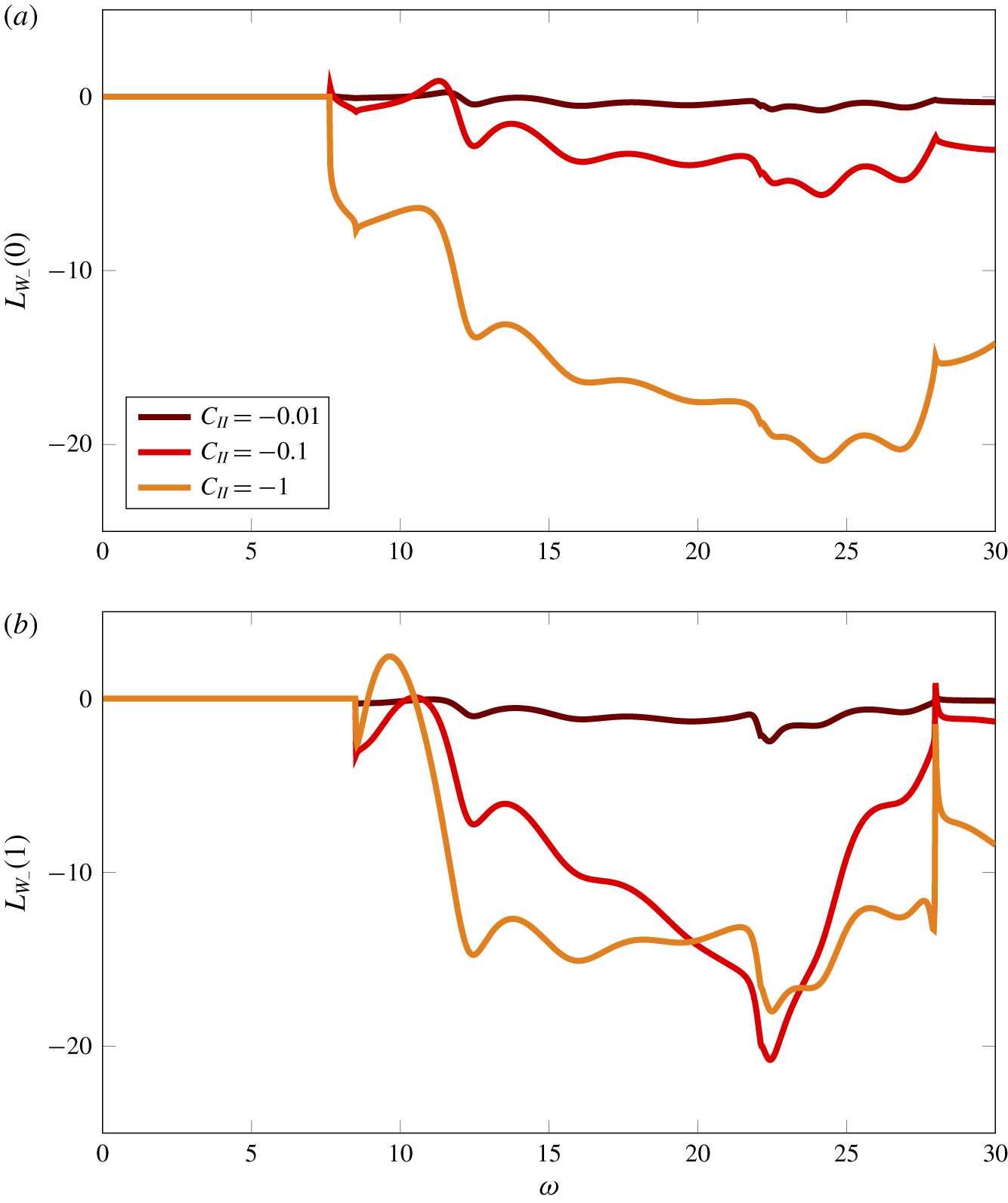
4.4 Sound transmission
We now use our model to investigate sound transmission through a cascade of flat plates with complex boundaries. Sound transmission occurs when a sound wave interacts with a cascade of blades, and is reflected and transmitted through the blade row. In order to explore the effects of modified boundary conditions on the transmission and reflection we write the incident acoustic field (2.6) in the form
 $$\begin{eqnarray}\displaystyle \unicode[STIX]{x1D719}_{i}=\text{e}^{\text{i}\unicode[STIX]{x1D701}_{0}^{-}y}\text{e}^{-\text{i}\unicode[STIX]{x1D706}_{0}^{-}x},\quad x\leqslant yd/s, & & \displaystyle \nonumber\end{eqnarray}$$
 where the mode is assumed cut-on, so that  $\unicode[STIX]{x1D706}_{0}$ is real. Comparison with the solution in § 3.1 shows that the reflected acoustic potential takes the form
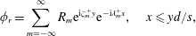 $$\begin{eqnarray}\displaystyle \unicode[STIX]{x1D719}_{r}=\mathop{\sum }_{m=-\infty }^{\infty }R_{m}\text{e}^{\text{i}\unicode[STIX]{x1D701}_{m}^{+}y}\text{e}^{-\text{i}\unicode[STIX]{x1D706}_{m}^{+}x},\quad x\leqslant yd/s, & & \displaystyle \nonumber\end{eqnarray}$$
and the transmitted acoustic potential takes the form
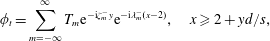 $$\begin{eqnarray}\displaystyle \unicode[STIX]{x1D719}_{t}=\mathop{\sum }_{m=-\infty }^{\infty }T_{m}\text{e}^{-\text{i}\unicode[STIX]{x1D701}_{m}^{-}y}\text{e}^{-\text{i}\unicode[STIX]{x1D706}_{m}^{-}(x-2)},\quad x\geqslant 2+yd/s, & & \displaystyle \nonumber\end{eqnarray}$$
 where  $R_{m}$ and $T_{m}$ are the reflection and transmission coefficients respectively. Note that the hydrodynamic mode ( $\unicode[STIX]{x1D714}/\unicode[STIX]{x1D6FD}^{2}$) corresponding to the jump in acoustic potential across the wake is not included in this analysis since it does not contribute to the pressure field.
By comparison with (3.12) and (3.13) we obtain the expressions for the transmission and reflection coefficients as
 $$\begin{eqnarray}\displaystyle R_{m}=+\frac{\unicode[STIX]{x03C0}\unicode[STIX]{x1D701}_{m}^{+}D^{(1,3)}(\unicode[STIX]{x1D706}_{m}^{+})}{\unicode[STIX]{x1D6E5}\sqrt{\unicode[STIX]{x1D714}^{2}w^{2}-f_{m}^{2}}},\quad T_{m}=-\frac{\unicode[STIX]{x03C0}\unicode[STIX]{x1D701}_{m}^{-}D^{(2,4)}(\unicode[STIX]{x1D706}_{m}^{-})}{\unicode[STIX]{x1D6E5}\sqrt{\unicode[STIX]{x1D714}^{2}w^{2}-f_{m}^{2}}}\text{e}^{-2\text{i}\unicode[STIX]{x1D706}_{m}^{-}}+\unicode[STIX]{x1D6FF}_{0,m}. & & \displaystyle \nonumber\end{eqnarray}$$
(ai–ci) The total (incident and scattered), normalised pressure field. (aii–cii) The amplitudes of the normalised reflection (blue) and transmission (orange) coefficients. The open area fraction values are  $\unicode[STIX]{x1D6FC}_{H}=0,0.01$ and $0.05$ respectively. The darker bars indicate modes that are cut-on whereas the lighter bars are cut-off. The parameters in this case are defined in case E of table 2. The arrow indicates the direction of the incident wave.
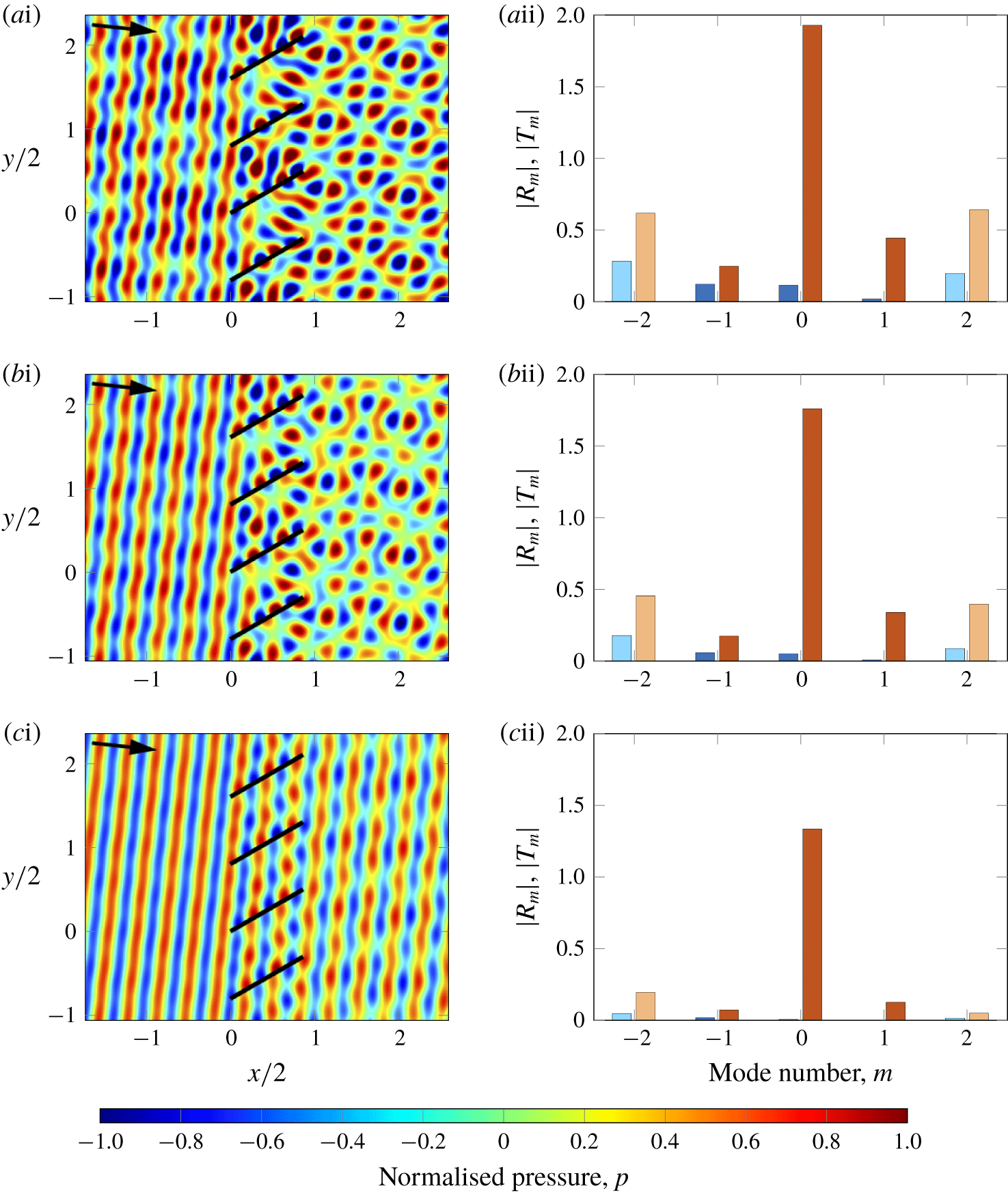
We now consider a practical example. Suppose that the blade is perforated with holes of radius  $R^{\ast }=0.02b^{\ast }$. We consider perturbations such that the pore-scale reduced frequency is $\unicode[STIX]{x1D714}_{P}=\unicode[STIX]{x1D714}^{\ast }R^{\ast }/U^{\ast }=2$, which corresponds to a reduced frequency of $\unicode[STIX]{x1D714}=100$ in our notation. Howe et al. (Reference Howe, Scott and Sipcic1996) calculated the components of the Rayleigh conductivity in this case to be $\unicode[STIX]{x1D6E4}_{R}=1.252$ and $\unicode[STIX]{x1D6E5}_{R}=0.705$, so that $K_{R}=0.0250{-}0.0141\text{i}$. The colormaps in figure 13(ai–ci) show the pressure field for three different open area fractions. The case 0 (rigid and impermeable) cascade shows significant diffraction and reflection of the incident wave, as indicated by the relatively large reflection and transmission coefficients in figure 13(aii). Increasing the open area fraction to the modest value of $\unicode[STIX]{x1D6FC}_{H}=0.01$ slightly decreases the strength of the reflected and transmitted waves, as evidenced in figure 13(bii). Increasing the open area fraction further to $\unicode[STIX]{x1D6FC}_{H}=0.05$ (figure 13cii) almost completely annihilates the backscattering. The effect is similar in the downstream field, though the open area fraction appears to have a slightly less significant effect, at least for the parameters we consider here. This asymmetry can be attributed to the Kutta condition. In contrast to the leading edge where the pressure is singular, at the trailing edge we require that the pressure jump vanishes. Accordingly, increasing the open area fraction cannot reduce the pressure jump by the same magnitude at the trailing edge as at the leading edge.
Since the Rayleigh conductivity has negative imaginary part, the incident perturbation transfers energy to the mean flow by means of the viscous action at the pore scale. Howe et al. (Reference Howe, Scott and Sipcic1996) provide a more detailed treatment of this phenomenon, and showed the perturbations can actually be amplified in certain frequency bands when the imaginary part of the Rayleigh conductivity is positive. This suggests that acoustic energy can only be absorbed by porous blades in certain frequency regimes, which is in accordance with numerical experiments we performed for the cascade.
5 Conclusions
We have derived an analytic solution for the scattering of an unsteady perturbation incident on a rectilinear cascade of flat blades with complex boundaries. The analytic nature of the solution means that it is extremely rapid to compute, and offers physical insight into the role played by different boundary conditions. In contrast with previous studies that focussed on the effects of rigid and impermeable blades (Glegg Reference Glegg1999; Posson et al. Reference Posson, Roger and Moreau2010), the formulation of the present research allows a range of boundary conditions to be studied with minimal effort, such as porosity, compliance and flow impedance. In terms of the spectral plane, the effect of modifying these boundary conditions is to change the locations of the zeros of the Wiener–Hopf kernel, whilst the poles are unchanged. Accordingly, the modal structure of the far-field scattered pressure is invariant under modifications to the flat blades’ boundary conditions. Conversely, the modal structure of the near-field region undergoes large deformations since the zeros of the kernel correspond to the duct modes of the inter-blade region. This has a strong effect on the surface pressure fluctuations and unsteady loading, which has implications for the far-field sound.
We have focussed on understanding the role of blade porosity. The results show that substantial reductions in both the unsteady lift and sound power output are possible for even modest values of porosity. At low frequencies we observe a significant change in the unsteady loading and a moderate effect on the sound power output. Conversely, at high frequencies we observe a significant effect on the sound power output and a small effect on the unsteady loading. Furthermore, the amplitudes of the reflection and transmission coefficients rapidly decrease as the blade porosity is increased. We attribute these considerable reductions to several physical mechanisms associated with porosity. Increasing the blade porosity promotes the communication between adjacent channels, which prevents large build-ups of pressure inside each channel. Moreover, the flow seepage afforded by porous channels permits the dissipation of energy through the blades, thus reducing unsteady pressure fluctuations on the blade. This reduction in pressure fluctuations corresponds to reductions in the scattered pressure and far-field sound. This study shows that modified boundary conditions can have a large impact on the generation and transmission of sound in cascades, and our analytic solution offers a useful design tool that models both aeroacoustic and aeroelastic effects. Future work will focus on understanding how surface treatments can be used to change the resonant frequency of a cascade to avoid lock-in and the associated structural damage.
Declaration of interests
The authors report no conflict of interest.
Appendix A. Wiener–Hopf solution
We now solve the integral equation (3.8) subject to the boundary conditions of no discontinuities upstream (2.7), a modified no-flux condition (2.17) and no pressure jump across the wake (2.20). In a similar way to Glegg (Reference Glegg1999), we split this problem into four coupled problems that are amenable to the Wiener–Hopf method.
We write
 $$\begin{eqnarray}\displaystyle \unicode[STIX]{x1D6E5}_{0}[\unicode[STIX]{x1D719}](x)=\unicode[STIX]{x1D6E5}_{0}[\unicode[STIX]{x1D719}^{(1)}](x)+\unicode[STIX]{x1D6E5}_{0}[\unicode[STIX]{x1D719}^{(2)}](x)+\unicode[STIX]{x1D6E5}_{0}[\unicode[STIX]{x1D719}^{(3)}](x)+\unicode[STIX]{x1D6E5}_{0}[\unicode[STIX]{x1D719}^{(4)}](x), & & \displaystyle\end{eqnarray}$$
and its Fourier transform
 $$\begin{eqnarray}\displaystyle D(\unicode[STIX]{x1D6FE})=D^{(1)}(\unicode[STIX]{x1D6FE})+D^{(2)}(\unicode[STIX]{x1D6FE})+D^{(3)}(\unicode[STIX]{x1D6FE})+D^{(4)}(\unicode[STIX]{x1D6FE}), & & \displaystyle\end{eqnarray}$$
 where each  $\unicode[STIX]{x1D6E5}_{0}[\unicode[STIX]{x1D719}^{(n)}]$ and $D^{(n)}$ satisfy a semi-infinite integral equation of the form
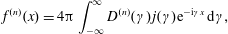 $$\begin{eqnarray}\displaystyle f^{(n)}(x)=4\unicode[STIX]{x03C0}\int _{-\infty }^{\infty }D^{(n)}(\unicode[STIX]{x1D6FE})j(\unicode[STIX]{x1D6FE})\text{e}^{-\text{i}\unicode[STIX]{x1D6FE}x}\,\text{d}\unicode[STIX]{x1D6FE}, & & \displaystyle\end{eqnarray}$$
 for  $n=1,2,3,4$. The corresponding boundary conditions are
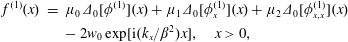 $$\begin{eqnarray}\displaystyle f^{(1)}(x) & = & \displaystyle \unicode[STIX]{x1D707}_{0}\unicode[STIX]{x1D6E5}_{0}[\unicode[STIX]{x1D719}^{(1)}](x)+\unicode[STIX]{x1D707}_{1}\unicode[STIX]{x1D6E5}_{0}[\unicode[STIX]{x1D719}_{x}^{(1)}](x)+\unicode[STIX]{x1D707}_{2}\unicode[STIX]{x1D6E5}_{0}[\unicode[STIX]{x1D719}_{x,x}^{(1)}](x)\nonumber\\ \displaystyle & & \displaystyle -\,2w_{0}\exp [\text{i}(k_{x}/\unicode[STIX]{x1D6FD}^{2})x],\quad x>0,\end{eqnarray}$$
 $$\begin{eqnarray}\displaystyle f^{(2)}(x)=\unicode[STIX]{x1D707}_{0}\unicode[STIX]{x1D6E5}_{0}[\unicode[STIX]{x1D719}^{(2)}](x)+\unicode[STIX]{x1D707}_{1}\unicode[STIX]{x1D6E5}_{0}[\unicode[STIX]{x1D719}_{x}^{(2)}](x)+\unicode[STIX]{x1D707}_{2}\unicode[STIX]{x1D6E5}_{0}[\unicode[STIX]{x1D719}_{x,x}^{(2)}](x),\quad x<2, & & \displaystyle\end{eqnarray}$$
 $$\begin{eqnarray}\displaystyle f^{(3)}(x)=\unicode[STIX]{x1D707}_{0}\unicode[STIX]{x1D6E5}_{0}[\unicode[STIX]{x1D719}^{(3)}](x)+\unicode[STIX]{x1D707}_{1}\unicode[STIX]{x1D6E5}_{0}[\unicode[STIX]{x1D719}_{x}^{(3)}](x)+\unicode[STIX]{x1D707}_{2}\unicode[STIX]{x1D6E5}_{0}[\unicode[STIX]{x1D719}_{x,x}^{(3)}](x),\quad x>0, & & \displaystyle\end{eqnarray}$$
 $$\begin{eqnarray}\displaystyle f^{(4)}(x)=\unicode[STIX]{x1D707}_{0}\unicode[STIX]{x1D6E5}_{0}[\unicode[STIX]{x1D719}^{(4)}](x)+\unicode[STIX]{x1D707}_{1}\unicode[STIX]{x1D6E5}_{0}[\unicode[STIX]{x1D719}_{x}^{(4)}](x)+\unicode[STIX]{x1D707}_{2}\unicode[STIX]{x1D6E5}_{0}[\unicode[STIX]{x1D719}_{x,x}^{(4)}](x),\quad x<2, & & \displaystyle\end{eqnarray}$$
and
 $$\begin{eqnarray}\displaystyle \unicode[STIX]{x1D6E5}_{0}[\unicode[STIX]{x1D719}^{(1)}](x)=0,\quad x<0, & & \displaystyle\end{eqnarray}$$
 $$\begin{eqnarray}\displaystyle \unicode[STIX]{x1D6E5}_{0}[\unicode[STIX]{x1D719}^{(1)}](x)+\unicode[STIX]{x1D6E5}_{0}[\unicode[STIX]{x1D719}^{(2)}](x)=2\unicode[STIX]{x03C0}\text{i}P^{(2)}\text{e}^{\text{i}(\unicode[STIX]{x1D714}/\unicode[STIX]{x1D6FD}^{2})x},\quad x>2, & & \displaystyle\end{eqnarray}$$
 $$\begin{eqnarray}\displaystyle \unicode[STIX]{x1D6E5}_{0}[\unicode[STIX]{x1D719}^{(2)}](x)+\unicode[STIX]{x1D6E5}_{0}[\unicode[STIX]{x1D719}^{(3)}](x)+\unicode[STIX]{x1D6E5}_{0}[\unicode[STIX]{x1D719}^{(4)}](x)=0,\quad x<0, & & \displaystyle\end{eqnarray}$$
 $$\begin{eqnarray}\displaystyle \unicode[STIX]{x1D6E5}_{0}[\unicode[STIX]{x1D719}^{(3)}](x)+\unicode[STIX]{x1D6E5}_{0}[\unicode[STIX]{x1D719}^{(4)}](x)=2\unicode[STIX]{x03C0}\text{i}P^{(4)}\text{e}^{\text{i}(\unicode[STIX]{x1D714}/\unicode[STIX]{x1D6FD}^{2})x},\quad x>2, & & \displaystyle\end{eqnarray}$$
 where  $P^{(2)}$ and $P^{(4)}$ are two constants of integration that will be specified to enforce the Kutta condition. Summing the four above conditions results in the original boundary conditions and, consequently, we may apply the Wiener–Hopf method to each semi-infinite integral equation and sum the resulting contributions to obtain a solution to the original equations.
A.1 Solution to first Wiener–Hopf equation –  $D^{(1)}$

In this section, we solve the integral equation (A 3) for  $n=1$
$n=1$
 $$\begin{eqnarray}\displaystyle f^{(1)}(x)=4\unicode[STIX]{x03C0}\int _{-\infty }^{\infty }D^{(1)}(\unicode[STIX]{x1D6FE})j(\unicode[STIX]{x1D6FE})\text{e}^{-\text{i}\unicode[STIX]{x1D6FE}x}\,\text{d}\unicode[STIX]{x1D6FE}, & & \displaystyle\end{eqnarray}$$
 subject to (A 4a) and (A 4b). Taking a Fourier transform of (A 8) in  $x$ gives
 $$\begin{eqnarray}\displaystyle F_{-}^{(1)}(\unicode[STIX]{x1D6FE})+F_{+}^{(1)}(\unicode[STIX]{x1D6FE})=4\unicode[STIX]{x03C0}D_{+}^{(1)}(\unicode[STIX]{x1D6FE})j(\unicode[STIX]{x1D6FE}), & & \displaystyle\end{eqnarray}$$
where
 $$\begin{eqnarray}\displaystyle F_{-}^{(1)}(\unicode[STIX]{x1D6FE})=\frac{1}{2\unicode[STIX]{x03C0}}\int _{-\infty }^{0}f^{(1)}(x)\text{e}^{\text{i}\unicode[STIX]{x1D6FE}x}\,\text{d}x,\quad F_{+}^{(1)}(\unicode[STIX]{x1D6FE})=\frac{1}{2\unicode[STIX]{x03C0}}\int _{0}^{\infty }f^{(1)}(x)\text{e}^{\text{i}\unicode[STIX]{x1D6FE}x}\,\text{d}x, & & \displaystyle\end{eqnarray}$$
 $$\begin{eqnarray}\displaystyle D_{+}^{(1)}(\unicode[STIX]{x1D6FE})=\int _{0}^{\infty }\unicode[STIX]{x1D6E5}_{0}[\unicode[STIX]{x1D719}^{(1)}](x)\text{e}^{\text{i}\unicode[STIX]{x1D6FE}x}\,\text{d}x. & & \displaystyle\end{eqnarray}$$
 The subscripts  $\pm$ here indicate that the functions are analytic in the upper or lower half planes, denoted by ${\mathcal{L}}^{\pm }$. We may employ (A 4a) to obtain
 $$\begin{eqnarray}\displaystyle F_{+}^{(1)}(\unicode[STIX]{x1D6FE})=\frac{w_{0}}{\unicode[STIX]{x03C0}\text{i}(\unicode[STIX]{x1D6FE}+k_{x}/\unicode[STIX]{x1D6FD}^{2})}+(\unicode[STIX]{x1D707}_{0}-\text{i}\unicode[STIX]{x1D707}_{1}\unicode[STIX]{x1D6FE}-\unicode[STIX]{x1D707}_{2}\unicode[STIX]{x1D6FE}^{2})D^{(1)}(\unicode[STIX]{x1D6FE}). & & \displaystyle \nonumber\end{eqnarray}$$
Consequently, the Wiener–Hopf equation (A 9) may be expressed as
 $$\begin{eqnarray}\displaystyle F_{-}^{(1)}(\unicode[STIX]{x1D6FE})+\frac{w_{0}}{\unicode[STIX]{x03C0}\text{i}(\unicode[STIX]{x1D6FE}+k_{x}/\unicode[STIX]{x1D6FD}^{2})}=4\unicode[STIX]{x03C0}D_{+}^{(1)}(\unicode[STIX]{x1D6FE})K(\unicode[STIX]{x1D6FE}), & & \displaystyle\end{eqnarray}$$
where
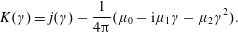 $$\begin{eqnarray}\displaystyle K(\unicode[STIX]{x1D6FE})=j(\unicode[STIX]{x1D6FE})-\frac{1}{4\unicode[STIX]{x03C0}}(\unicode[STIX]{x1D707}_{0}-\text{i}\unicode[STIX]{x1D707}_{1}\unicode[STIX]{x1D6FE}-\unicode[STIX]{x1D707}_{2}\unicode[STIX]{x1D6FE}^{2}). & & \displaystyle\end{eqnarray}$$
 The multiplicative splitting  $K=K_{+}K_{-}$ is performed in appendix B. This splitting enables us to write
 $$\begin{eqnarray}\displaystyle \frac{F_{-}^{(1)}(\unicode[STIX]{x1D6FE})}{K_{-}(\unicode[STIX]{x1D6FE})}+\frac{w_{0}}{\unicode[STIX]{x03C0}\text{i}(\unicode[STIX]{x1D6FE}+k_{x}/\unicode[STIX]{x1D6FD}^{2})K_{-}(\unicode[STIX]{x1D6FE})}=4\unicode[STIX]{x03C0}D_{+}^{(1)}(\unicode[STIX]{x1D6FE})K_{+}(\unicode[STIX]{x1D6FE}). & & \displaystyle\end{eqnarray}$$
We now additively factorise the left side of (A 13). We apply pole removal (Noble Reference Noble1958) to obtain the additive splitting
 $$\begin{eqnarray}\displaystyle \frac{1}{(\unicode[STIX]{x1D6FE}+k_{x}/\unicode[STIX]{x1D6FD}^{2})K_{-}(\unicode[STIX]{x1D6FE})} & = & \displaystyle \underbrace{\frac{1}{(\unicode[STIX]{x1D6FE}+k_{x}/\unicode[STIX]{x1D6FD}^{2})K_{-}(-k_{x}/\unicode[STIX]{x1D6FD}^{2})}}_{+}\nonumber\\ \displaystyle & & \displaystyle +\,\underbrace{\frac{1}{(\unicode[STIX]{x1D6FE}+k_{x}/\unicode[STIX]{x1D6FD}^{2})K_{-}(\unicode[STIX]{x1D6FE})}-\frac{1}{(\unicode[STIX]{x1D6FE}+k_{x}/\unicode[STIX]{x1D6FD}^{2})K_{-}(-k_{x}/\unicode[STIX]{x1D6FD}^{2})}}_{-},\nonumber\end{eqnarray}$$
 where the underbrace  $\pm$ denotes that the function is analytic in ${\mathcal{L}}^{\pm }$ respectively. Therefore, (A 11) becomes
 $$\begin{eqnarray}\displaystyle & & \displaystyle \frac{F_{-}^{(1)}(\unicode[STIX]{x1D6FE})}{K_{-}(\unicode[STIX]{x1D6FE})}+\frac{w_{0}}{\unicode[STIX]{x03C0}\text{i}(\unicode[STIX]{x1D6FE}+k_{x}/\unicode[STIX]{x1D6FD}^{2})K_{-}(\unicode[STIX]{x1D6FE})}-\frac{w_{0}}{\unicode[STIX]{x03C0}\text{i}(\unicode[STIX]{x1D6FE}+k_{x}/\unicode[STIX]{x1D6FD}^{2})K_{-}(-k_{x}/\unicode[STIX]{x1D6FD}^{2})}\nonumber\\ \displaystyle & & \displaystyle \qquad \quad =4\unicode[STIX]{x03C0}D_{+}^{(1)}(\unicode[STIX]{x1D6FE})K_{+}(\unicode[STIX]{x1D6FE})-\frac{w_{0}}{\unicode[STIX]{x03C0}\text{i}(\unicode[STIX]{x1D6FE}+k_{x}/\unicode[STIX]{x1D6FD}^{2})K_{-}(-k_{x}/\unicode[STIX]{x1D6FD}^{2})}.\end{eqnarray}$$
 We may now apply the standard Wiener–Hopf argument: since the left and right sides of (A 14) are analytic in  ${\mathcal{L}}^{\mp }$ respectively, and they agree on a strip, each side defines the analytic continuation of the other. Therefore, equation (A 14) defines an entire function, $E_{1}(\unicode[STIX]{x1D6FE})$. As $|\unicode[STIX]{x1D6FE}|\rightarrow \infty$ in ${\mathcal{L}}^{-}$, the left side of (A 14) decays. This can be seen by considering the growth of $K_{-}$, which is explicated in appendix B. Similarly, as $|\unicode[STIX]{x1D6FE}|\rightarrow \infty$ in ${\mathcal{L}}^{+}$, the right side of (A 14) vanishes. Therefore, $E_{1}(\unicode[STIX]{x1D6FE})$ is bounded in the entire plane and must be constant according to Liouville’s theorem. Moreover, since $E_{1}(\unicode[STIX]{x1D6FE})$ decays, this constant must be zero. Finally, we rearrange the right side of (A 14) to obtain the solution to the first Wiener–Hopf problem as
 $$\begin{eqnarray}\displaystyle D^{(1)}(\unicode[STIX]{x1D6FE})=\frac{w_{0}}{(2\unicode[STIX]{x03C0})^{2}\text{i}(\unicode[STIX]{x1D6FE}+k_{x}/\unicode[STIX]{x1D6FD}^{2})K_{-}(-k_{x}/\unicode[STIX]{x1D6FD}^{2})K_{+}(\unicode[STIX]{x1D6FE})}. & & \displaystyle\end{eqnarray}$$
A.2 Solution to second Wiener–Hopf equation – $D^{(2)}$

In this section we solve the integral equation (A 3) for  $n=2$,
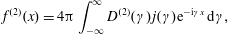 $$\begin{eqnarray}\displaystyle f^{(2)}(x)=4\unicode[STIX]{x03C0}\int _{-\infty }^{\infty }D^{(2)}(\unicode[STIX]{x1D6FE})j(\unicode[STIX]{x1D6FE})\text{e}^{-\text{i}\unicode[STIX]{x1D6FE}x}\,\text{d}\unicode[STIX]{x1D6FE}, & & \displaystyle\end{eqnarray}$$
subject to (A 5a) and (A 5b). Taking a Fourier transform of (A 16a) and applying (A 5a) yields
 $$\begin{eqnarray}\displaystyle (\unicode[STIX]{x1D707}_{0}-\text{i}\unicode[STIX]{x1D707}_{1}\unicode[STIX]{x1D6FE}-\unicode[STIX]{x1D707}_{2}\unicode[STIX]{x1D6FE}^{2})D^{(1)}(\unicode[STIX]{x1D6FE})+F_{+}^{(2)}(\unicode[STIX]{x1D6FE})=4\unicode[STIX]{x03C0}(D_{-}^{(2)}(\unicode[STIX]{x1D6FE})+D_{+}^{(2)}(\unicode[STIX]{x1D6FE}))j(\unicode[STIX]{x1D6FE}), & & \displaystyle\end{eqnarray}$$
where
 $$\begin{eqnarray}\displaystyle & \displaystyle F_{+}^{(2)}(\unicode[STIX]{x1D6FE})=\frac{1}{2\unicode[STIX]{x03C0}}\int _{2}^{\infty }f^{(2)}(x)\text{e}^{\text{i}\unicode[STIX]{x1D6FE}x}\,\text{d}x=\frac{\text{e}^{2\text{i}\unicode[STIX]{x1D6FE}}}{2\unicode[STIX]{x03C0}}\int _{0}^{\infty }f^{(2)}(x+2)\text{e}^{\text{i}x\unicode[STIX]{x1D6FE}}\,\text{d}x=\text{e}^{2\text{i}\unicode[STIX]{x1D6FE}}F_{+}^{\ast (2)}(\unicode[STIX]{x1D6FE}),\qquad & \displaystyle\end{eqnarray}$$
 $$\begin{eqnarray}\displaystyle & \displaystyle D_{+}^{(2)}(\unicode[STIX]{x1D6FE})=\frac{1}{2\unicode[STIX]{x03C0}}\int _{2}^{\infty }\unicode[STIX]{x1D6E5}_{0}[\unicode[STIX]{x1D719}^{(2)}](x)\text{e}^{\text{i}\unicode[STIX]{x1D6FE}x}\,\text{d}x=\frac{\text{e}^{2\text{i}\unicode[STIX]{x1D6FE}}}{2\unicode[STIX]{x03C0}}\int _{0}^{\infty }\unicode[STIX]{x1D6E5}_{0}[\unicode[STIX]{x1D719}^{(2)}](x+2)\text{e}^{\text{i}x\unicode[STIX]{x1D6FE}}\,\text{d}x=\text{e}^{2\text{i}\unicode[STIX]{x1D6FE}}D_{+}^{\ast (2)}(\unicode[STIX]{x1D6FE}), & \displaystyle \nonumber\\ \displaystyle & & \displaystyle\end{eqnarray}$$
 $$\begin{eqnarray}\displaystyle & \displaystyle D_{-}^{(2)}(\unicode[STIX]{x1D6FE})=\frac{1}{2\unicode[STIX]{x03C0}}\int _{-\infty }^{2}\unicode[STIX]{x1D6E5}_{0}[\unicode[STIX]{x1D719}^{(2)}](x)\text{e}^{\text{i}\unicode[STIX]{x1D6FE}x}\,\text{d}x=\frac{\text{e}^{2\text{i}\unicode[STIX]{x1D6FE}}}{2\unicode[STIX]{x03C0}}\int _{-\infty }^{0}\unicode[STIX]{x1D6E5}_{0}[\unicode[STIX]{x1D719}^{(2)}](x+2)\text{e}^{\text{i}x\unicode[STIX]{x1D6FE}}\,\text{d}x=\text{e}^{2\text{i}\unicode[STIX]{x1D6FE}}D_{-}^{\ast (2)}(\unicode[STIX]{x1D6FE}). & \displaystyle \nonumber\\ \displaystyle & & \displaystyle\end{eqnarray}$$ $\text{e}^{2\text{i}\unicode[STIX]{x1D6FE}}$ dependence and employing (A 12) transforms the Wiener–Hopf equation (A 19) to
  $$\begin{eqnarray}\displaystyle F_{+}^{\ast (2)}(\unicode[STIX]{x1D6FE})=4\unicode[STIX]{x03C0}(D_{-}^{\ast (2)}(\unicode[STIX]{x1D6FE})+D_{+}^{\ast (2)}(\unicode[STIX]{x1D6FE}))K(\unicode[STIX]{x1D6FE}), & & \displaystyle\end{eqnarray}$$
 and we may use the multiplicative splitting of  $K$ to write
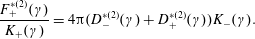 $$\begin{eqnarray}\displaystyle \frac{F_{+}^{\ast (2)}(\unicode[STIX]{x1D6FE})}{K_{+}(\unicode[STIX]{x1D6FE})}=4\unicode[STIX]{x03C0}(D_{-}^{\ast (2)}(\unicode[STIX]{x1D6FE})+D_{+}^{\ast (2)}(\unicode[STIX]{x1D6FE}))K_{-}(\unicode[STIX]{x1D6FE}). & & \displaystyle\end{eqnarray}$$
We may use the downstream boundary condition for this problem (A 5b) to write
 $$\begin{eqnarray}\displaystyle D_{+}^{\ast (2)}(\unicode[STIX]{x1D6FE})=-\frac{P^{\ast (2)}}{\unicode[STIX]{x1D6FE}+\unicode[STIX]{x1D714}/\unicode[STIX]{x1D6FD}^{2}}-\frac{1}{2\unicode[STIX]{x03C0}}\int _{0}^{\infty }\unicode[STIX]{x1D6E5}_{0}[\unicode[STIX]{x1D719}^{(1)}](x+2)\text{e}^{\text{i}\unicode[STIX]{x1D6FE}x}\,\text{d}x. & & \displaystyle\end{eqnarray}$$
 where  $P^{\ast (2)}=P^{(2)}\text{e}^{2\text{i}k_{x}/\unicode[STIX]{x1D6FD}^{2}}$. To calculate the remaining integral we use the inversion formula for the Fourier transform
 $$\begin{eqnarray}\displaystyle \unicode[STIX]{x1D6E5}_{0}[\unicode[STIX]{x1D719}^{(1)}](x)=\int _{-\infty -\text{i}\unicode[STIX]{x1D70F}_{1}}^{\infty -\text{i}\unicode[STIX]{x1D70F}_{1}}D^{(1)}(\unicode[STIX]{x1D6FE})\text{e}^{-\text{i}\unicode[STIX]{x1D6FE}x}\,\text{d}\unicode[STIX]{x1D6FE}, & & \displaystyle \nonumber\end{eqnarray}$$
 for some  $\unicode[STIX]{x1D70F}_{1}>0$. By substituting this representation into our desired integral, we obtain
 $$\begin{eqnarray}\displaystyle \frac{1}{2\unicode[STIX]{x03C0}}\int _{0}^{\infty }\unicode[STIX]{x1D6E5}_{0}[\unicode[STIX]{x1D719}^{(1)}](x+2)\text{e}^{\text{i}\unicode[STIX]{x1D6FE}x}\,\text{d}x=\frac{1}{2\unicode[STIX]{x03C0}}\int _{0}^{\infty }\int _{-\infty -\text{i}\unicode[STIX]{x1D70F}_{1}}^{\infty -\text{i}\unicode[STIX]{x1D70F}_{1}}D^{(1)}(\unicode[STIX]{x1D6FE}_{1})\text{e}^{-\text{i}\unicode[STIX]{x1D6FE}_{1}(x+2)}\,\text{d}\unicode[STIX]{x1D6FE}_{1}\text{e}^{\text{i}\unicode[STIX]{x1D6FE}x}\,\text{d}x. & & \displaystyle \nonumber\end{eqnarray}$$
 Rearranging the order of integration and computing the resulting  $x$-integral results in
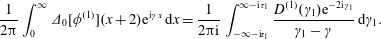 $$\begin{eqnarray}\displaystyle \frac{1}{2\unicode[STIX]{x03C0}}\int _{0}^{\infty }\unicode[STIX]{x1D6E5}_{0}[\unicode[STIX]{x1D719}^{(1)}](x+2)\text{e}^{\text{i}\unicode[STIX]{x1D6FE}x}\,\text{d}x=\frac{1}{2\unicode[STIX]{x03C0}\text{i}}\int _{-\infty -\text{i}\unicode[STIX]{x1D70F}_{1}}^{\infty -\text{i}\unicode[STIX]{x1D70F}_{1}}\frac{D^{(1)}(\unicode[STIX]{x1D6FE}_{1})\text{e}^{-2\text{i}\unicode[STIX]{x1D6FE}_{1}}}{\unicode[STIX]{x1D6FE}_{1}-\unicode[STIX]{x1D6FE}}\,\text{d}\unicode[STIX]{x1D6FE}_{1}. & & \displaystyle\end{eqnarray}$$
 Since  $d<2$, we may close the remaining integral in ${\mathcal{L}}^{-}$. There are no branches in the integrand so the integral consists of the residues of simple poles at $\unicode[STIX]{x1D6FE}=-k_{x}/\unicode[STIX]{x1D6FD}^{2}$, $\unicode[STIX]{x1D703}_{n}^{-}$. Consequently, inserting (A 15) into the above integral yields
 $$\begin{eqnarray}\displaystyle & & \displaystyle \frac{1}{2\unicode[STIX]{x03C0}\text{i}}\int _{-\infty -\text{i}\unicode[STIX]{x1D70F}_{1}}^{\infty -\text{i}\unicode[STIX]{x1D70F}_{1}}\frac{1}{(\unicode[STIX]{x1D6FE}+k_{x}/\unicode[STIX]{x1D6FD}^{2})K_{-}(-k_{x}/\unicode[STIX]{x1D6FD}^{2})K_{+}(\unicode[STIX]{x1D6FE})}\,\frac{\text{e}^{-2\text{i}\unicode[STIX]{x1D6FE}_{1}}}{\unicode[STIX]{x1D6FE}_{1}-\unicode[STIX]{x1D6FE}}\,\text{d}\unicode[STIX]{x1D6FE}_{1}\nonumber\\ \displaystyle & & \displaystyle \quad =\frac{\text{e}^{2\text{i}k_{x}/\unicode[STIX]{x1D6FD}^{2}}}{(\unicode[STIX]{x1D6FE}+k_{x}/\unicode[STIX]{x1D6FD}^{2})K(-k_{x}/\unicode[STIX]{x1D6FD}^{2})}+\mathop{\sum }_{n=0}^{\infty }\frac{\text{e}^{-2\text{i}\unicode[STIX]{x1D703}_{n}^{-}}}{(\unicode[STIX]{x1D703}_{n}^{-}+k_{x}/\unicode[STIX]{x1D6FD}^{2})K_{-}(-k_{x}/\unicode[STIX]{x1D6FD}^{2})K_{+}^{\prime }(\unicode[STIX]{x1D703}_{n}^{-})(\unicode[STIX]{x1D6FE}-\unicode[STIX]{x1D703}_{n}^{-})},\nonumber\end{eqnarray}$$
 where the derivatives of  $K_{\pm }$ evaluated at the duct modes $\unicode[STIX]{x1D703}_{n}^{\mp }$ are given by
 $$\begin{eqnarray}\displaystyle K_{\pm }^{\prime }(\unicode[STIX]{x1D703}_{n}^{\mp }) & = & \displaystyle \frac{K^{\prime }(\unicode[STIX]{x1D703}_{n}^{\mp })}{K_{\mp }(\unicode[STIX]{x1D703}_{n}^{\mp })}=\frac{1}{4\unicode[STIX]{x03C0}K_{\mp }(\unicode[STIX]{x1D703}_{n}^{\mp })}\left(-\frac{(\unicode[STIX]{x1D703}_{n}^{\mp }/\unicode[STIX]{x1D701}(\unicode[STIX]{x1D703}_{n}^{\mp }))\sin (s\unicode[STIX]{x1D701}(\unicode[STIX]{x1D703}_{n}^{\mp }))+s\unicode[STIX]{x1D703}_{n}^{\mp }\cos (s\unicode[STIX]{x1D701}(\unicode[STIX]{x1D703}_{n}^{\mp }))}{\cos (s\unicode[STIX]{x1D701}(\unicode[STIX]{x1D703}_{n}^{\mp }))-\cos (d\unicode[STIX]{x1D703}_{n}^{\mp }+\unicode[STIX]{x1D70E}^{\prime })}\right.\nonumber\\ \displaystyle & & \displaystyle \quad -\,\frac{\unicode[STIX]{x1D703}_{n}^{\mp }s\sin (s\unicode[STIX]{x1D701}(\unicode[STIX]{x1D703}_{n}^{\mp }))^{2}+d\unicode[STIX]{x1D701}(\unicode[STIX]{x1D703}_{n}^{\mp })\sin (d\unicode[STIX]{x1D703}_{n}^{\mp }+\unicode[STIX]{x1D70E}^{\prime })\sin (s\unicode[STIX]{x1D701}(\unicode[STIX]{x1D703}_{n}^{\mp }))}{(\cos (s\unicode[STIX]{x1D701}(\unicode[STIX]{x1D703}_{n}^{\mp }))-\cos (d\unicode[STIX]{x1D703}_{n}^{\mp }+\unicode[STIX]{x1D70E}^{\prime }))^{2}}\nonumber\\ \displaystyle & & \displaystyle \quad +\left.\text{i}\unicode[STIX]{x1D707}_{1}+2\unicode[STIX]{x1D707}_{2}\unicode[STIX]{x1D703}_{n}^{\mp }\right).\nonumber\end{eqnarray}$$
Therefore, substitution of (A 22) into (A 21) yields
 $$\begin{eqnarray}\displaystyle D_{+}^{\ast (2)}(\unicode[STIX]{x1D6FE}) & = & \displaystyle \frac{w_{0}\text{e}^{2\text{i}k_{x}/\unicode[STIX]{x1D6FD}^{2}}}{(2\unicode[STIX]{x03C0})^{2}\text{i}(\unicode[STIX]{x1D6FE}+k_{x}/\unicode[STIX]{x1D6FD}^{2})K(-k_{x}/\unicode[STIX]{x1D6FD}^{2})}-\mathop{\sum }_{n=0}^{\infty }\frac{{\mathcal{A}}_{n}\text{e}^{-2\text{i}\unicode[STIX]{x1D703}_{n}^{-}}}{\text{i}(\unicode[STIX]{x1D703}_{n}^{-}+\unicode[STIX]{x1D714}/\unicode[STIX]{x1D6FD}^{2})(\unicode[STIX]{x1D6FE}-\unicode[STIX]{x1D703}_{n}^{-})},\nonumber\\ \displaystyle & & \displaystyle -\,\frac{P^{\ast (2)}}{\unicode[STIX]{x1D6FE}+\unicode[STIX]{x1D714}/\unicode[STIX]{x1D6FD}^{2}},\end{eqnarray}$$
where
 $$\begin{eqnarray}\displaystyle {\mathcal{A}}_{n}=\frac{w_{0}(\unicode[STIX]{x1D703}_{n}^{-}+\unicode[STIX]{x1D714}/\unicode[STIX]{x1D6FD}^{2})}{(2\unicode[STIX]{x03C0})^{2}(\unicode[STIX]{x1D703}_{n}^{-}+k_{x}/\unicode[STIX]{x1D6FD}^{2})K_{-}(-k_{x}/\unicode[STIX]{x1D6FD}^{2})K_{+}^{\prime }(\unicode[STIX]{x1D703}_{n}^{-})}. & & \displaystyle \nonumber\end{eqnarray}$$
We use the notation
 $$\begin{eqnarray}\displaystyle \tilde{K}_{-}(\unicode[STIX]{x1D6FE},\unicode[STIX]{x1D702}^{-})\triangleq \frac{K_{-}(\unicode[STIX]{x1D6FE})}{\unicode[STIX]{x1D6FE}-\unicode[STIX]{x1D702}^{-}}, & & \displaystyle \nonumber\end{eqnarray}$$
so that substitution of (A 23) into the Wiener–Hopf equation (A 17) yields
 $$\begin{eqnarray}\displaystyle \frac{F_{+}^{\ast (2)}(\unicode[STIX]{x1D6FE})}{4\unicode[STIX]{x03C0}K_{+}(\unicode[STIX]{x1D6FE})} & = & \displaystyle K_{-}(\unicode[STIX]{x1D6FE})D_{-}^{\ast (2)}(\unicode[STIX]{x1D6FE})-P^{\ast (2)}\tilde{K}_{-}(\unicode[STIX]{x1D6FE},-\unicode[STIX]{x1D714}/\unicode[STIX]{x1D6FD}^{2})\nonumber\\ \displaystyle & & \displaystyle +\,\frac{w_{0}\text{e}^{2\text{i}k_{x}/\unicode[STIX]{x1D6FD}^{2}}}{(2\unicode[STIX]{x03C0})^{2}\text{i}}\,\frac{\tilde{K}_{-}(\unicode[STIX]{x1D6FE},-k_{x}/\unicode[STIX]{x1D6FD}^{2})}{K(-k_{x}/\unicode[STIX]{x1D6FD}^{2})}-\mathop{\sum }_{n=0}^{\infty }\frac{{\mathcal{A}}_{n}\text{e}^{-2\text{i}\unicode[STIX]{x1D703}_{n}^{-}}}{\text{i}(\unicode[STIX]{x1D703}_{n}^{-}+\unicode[STIX]{x1D714}/\unicode[STIX]{x1D6FD}^{2})}\tilde{K}_{-}(\unicode[STIX]{x1D6FE},\unicode[STIX]{x1D703}_{n}^{-}).\qquad\end{eqnarray}$$
We note the additive splitting
 $$\begin{eqnarray}\displaystyle \tilde{K}_{-}(\unicode[STIX]{x1D6FE},\unicode[STIX]{x1D702}^{-})=[\tilde{K}_{-}(\unicode[STIX]{x1D6FE},\unicode[STIX]{x1D702})]_{+}+[\tilde{K}_{-}(\unicode[STIX]{x1D6FE},\unicode[STIX]{x1D702})]_{-}, & & \displaystyle\end{eqnarray}$$
where
 $$\begin{eqnarray}\displaystyle [\tilde{K}_{-}(\unicode[STIX]{x1D6FE},\unicode[STIX]{x1D702})]_{+}=\frac{K_{-}(\unicode[STIX]{x1D702}^{-})}{\unicode[STIX]{x1D6FE}-\unicode[STIX]{x1D702}^{-}},\quad [\tilde{K}_{-}(\unicode[STIX]{x1D6FE},\unicode[STIX]{x1D702})]_{-}=\frac{K_{-}(\unicode[STIX]{x1D6FE})-K_{-}(\unicode[STIX]{x1D702}^{-})}{\unicode[STIX]{x1D6FE}-\unicode[STIX]{x1D702}^{-}}. & & \displaystyle \nonumber\end{eqnarray}$$
Substituting these splittings into (A 24) yields
 $$\begin{eqnarray}\displaystyle & & \displaystyle \frac{F_{+}^{\ast (2)}(\unicode[STIX]{x1D6FE})}{4\unicode[STIX]{x03C0}K_{+}(\unicode[STIX]{x1D6FE})}+P^{\ast (2)}[\tilde{K}_{-}(\unicode[STIX]{x1D6FE},-\unicode[STIX]{x1D714}/\unicode[STIX]{x1D6FD}^{2})]_{+}-\frac{w_{0}\text{e}^{2\text{i}k_{x}/\unicode[STIX]{x1D6FD}^{2}}}{(2\unicode[STIX]{x03C0})^{2}\text{i}}\,\frac{[\tilde{K}_{-}(\unicode[STIX]{x1D6FE},-k_{x}/\unicode[STIX]{x1D6FD}^{2})]_{+}}{K(-k_{x}/\unicode[STIX]{x1D6FD}^{2})}\nonumber\\ \displaystyle & & \displaystyle \quad +\,\mathop{\sum }_{n=0}^{\infty }\frac{{\mathcal{A}}_{n}\text{e}^{-2\text{i}\unicode[STIX]{x1D703}_{n}^{-}}}{\text{i}(\unicode[STIX]{x1D703}_{n}^{-}+\unicode[STIX]{x1D714}/\unicode[STIX]{x1D6FD}^{2})}[\tilde{K}_{-}(\unicode[STIX]{x1D6FE},\unicode[STIX]{x1D703}_{n}^{-})]_{+}=K_{-}(\unicode[STIX]{x1D6FE})D_{-}^{\ast (2)}(\unicode[STIX]{x1D6FE})-P^{\ast (2)}[\tilde{K}_{-}(\unicode[STIX]{x1D6FE},-\unicode[STIX]{x1D714}/\unicode[STIX]{x1D6FD}^{2})]_{-}\nonumber\\ \displaystyle & & \displaystyle \quad +\,\frac{w_{0}\text{e}^{2\text{i}k_{x}/\unicode[STIX]{x1D6FD}^{2}}}{(2\unicode[STIX]{x03C0})^{2}\text{i}}\,\frac{[\tilde{K}_{-}(\unicode[STIX]{x1D6FE},-k_{x}/\unicode[STIX]{x1D6FD}^{2})]_{-}}{K(-k_{x}/\unicode[STIX]{x1D6FD}^{2})}-\mathop{\sum }_{n=0}^{\infty }\frac{{\mathcal{A}}_{n}\text{e}^{-2\text{i}\unicode[STIX]{x1D703}_{n}^{-}}}{\text{i}(\unicode[STIX]{x1D703}_{n}^{-}+\unicode[STIX]{x1D714}/\unicode[STIX]{x1D6FD}^{2})}[\tilde{K}_{-}(\unicode[STIX]{x1D6FE},\unicode[STIX]{x1D703}_{n}^{-})]_{-}.\end{eqnarray}$$
 In a similar way to § A.1, we now apply the typical Wiener–Hopf argument. We enforce the unsteady Kutta condition (Ayton, Gill & Peake Reference Ayton, Gill and Peake2016) which restricts the pressure at the trailing edge to be finite. Consequently, and using the results of appendix B, the left side of (A 26) decays as  $|\unicode[STIX]{x1D6FE}|\rightarrow \infty$ in ${\mathcal{L}}^{+}$ and the left side of (A 26) tends to an unknown constant as $|\unicode[STIX]{x1D6FE}|\rightarrow \infty$ in ${\mathcal{L}}^{-}$. Applying analytic continuation and Liouville’s theorem determines that this constant must be zero. Accordingly, the coefficient of $\unicode[STIX]{x1D6FE}^{-1}$ on the left side of (A 26) must vanish so that
 $$\begin{eqnarray}\displaystyle P^{\ast (2)}=\frac{w_{0}\text{e}^{2\text{i}k_{x}/\unicode[STIX]{x1D6FD}^{2}}}{(2\unicode[STIX]{x03C0})^{2}\text{i}K_{+}(-k_{x}/\unicode[STIX]{x1D6FD}^{2})}\,\frac{1}{K_{-}(-\unicode[STIX]{x1D714}/\unicode[STIX]{x1D6FD}^{2})}-\mathop{\sum }_{n=0}^{\infty }\frac{{\mathcal{A}}_{n}\text{e}^{-2\text{i}\unicode[STIX]{x1D703}_{n}^{-}}}{\text{i}(\unicode[STIX]{x1D703}_{n}^{-}+\unicode[STIX]{x1D714}/\unicode[STIX]{x1D6FD}^{2})}\,\frac{K_{-}(\unicode[STIX]{x1D703}_{n}^{-})}{K_{-}(-\unicode[STIX]{x1D714}/\unicode[STIX]{x1D6FD}^{2})}. & & \displaystyle \nonumber\end{eqnarray}$$
So that, after substituting in the downstream representation (A 23) and the above expression for the pressure constant, the right side of (A 26) yields
 $$\begin{eqnarray}\displaystyle D^{(2)}(\unicode[STIX]{x1D6FE}) & = & \displaystyle \frac{w_{0}(\unicode[STIX]{x1D714}-k_{x})\text{e}^{2\text{i}(\unicode[STIX]{x1D6FE}+k_{x}/\unicode[STIX]{x1D6FD}^{2})}}{(2\unicode[STIX]{x03C0}\unicode[STIX]{x1D6FD})^{2}\text{i}(\unicode[STIX]{x1D6FE}+k_{x}/\unicode[STIX]{x1D6FD}^{2})(\unicode[STIX]{x1D6FE}+\unicode[STIX]{x1D714}/\unicode[STIX]{x1D6FD}^{2})K_{+}(-k_{x}/\unicode[STIX]{x1D6FD}^{2})}\,\frac{1}{K_{-}(\unicode[STIX]{x1D6FE})}\nonumber\\ \displaystyle & & \displaystyle -\,\mathop{\sum }_{n=0}^{\infty }\frac{{\mathcal{A}}_{n}\text{e}^{2\text{i}(\unicode[STIX]{x1D6FE}-\unicode[STIX]{x1D703}_{n}^{-})}}{\text{i}(\unicode[STIX]{x1D6FE}+\unicode[STIX]{x1D714}/\unicode[STIX]{x1D6FD}^{2})(\unicode[STIX]{x1D6FE}-\unicode[STIX]{x1D703}_{n}^{-})}\,\frac{K_{-}(\unicode[STIX]{x1D703}_{n}^{-})}{K_{-}(\unicode[STIX]{x1D6FE})}.\end{eqnarray}$$
 It should be noted that the only poles of  $D^{(2)}$ in ${\mathcal{L}}^{+}$ are at the zeros of $K_{-}$.
A.3 Solution to third and fourth Wiener–Hopf equations – $D^{(3)},D^{(4)}$

Since the integral equations for  $\unicode[STIX]{x1D6E5}_{0}[\unicode[STIX]{x1D719}^{(3)}]$ and $\unicode[STIX]{x1D6E5}_{0}[\unicode[STIX]{x1D719}^{(4)}]$ are coupled, we must solve for them simultaneously. Taking a Fourier Transform of (A 3) and applying the boundary conditions for (A 6a) and (A 7a) for $n=3,4$ gives
 $$\begin{eqnarray}\displaystyle & \displaystyle F_{-}^{(3)}(\unicode[STIX]{x1D6FE})=4\unicode[STIX]{x03C0}[D_{-}^{(3)}(\unicode[STIX]{x1D6FE})+D_{+}^{(3)}(\unicode[STIX]{x1D6FE})]K(\unicode[STIX]{x1D6FE}), & \displaystyle\end{eqnarray}$$
 $$\begin{eqnarray}\displaystyle & \displaystyle F_{+}^{\ast (4)}(\unicode[STIX]{x1D6FE})=4\unicode[STIX]{x03C0}[D_{-}^{\ast (4)}(\unicode[STIX]{x1D6FE})+D_{+}^{\ast (4)}(\unicode[STIX]{x1D6FE})]K(\unicode[STIX]{x1D6FE}), & \displaystyle\end{eqnarray}$$
 where  $F_{-}^{(3)}$, $D_{-}^{(3)}$ and $D_{+}^{(3)}$ are defined in an analogous way to (A 10a,b) and (A 10c), and $F_{+}^{\ast (4)}$, $D_{+}^{\ast (4)}$ and $D_{-}^{\ast (4)}$ are defined in an analogous way to (A 18a), (A 18b) and (A 18c). Using a similar approach to § A.2, the upstream boundary condition (A 6b) may be expressed as
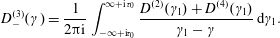 $$\begin{eqnarray}\displaystyle D_{-}^{(3)}(\unicode[STIX]{x1D6FE})=\frac{1}{2\unicode[STIX]{x03C0}\text{i}}\int _{-\infty +\text{i}\unicode[STIX]{x1D70F}_{0}}^{\infty +\text{i}\unicode[STIX]{x1D70F}_{0}}\frac{D^{(2)}(\unicode[STIX]{x1D6FE}_{1})+D^{(4)}(\unicode[STIX]{x1D6FE}_{1})}{\unicode[STIX]{x1D6FE}_{1}-\unicode[STIX]{x1D6FE}}\,\text{d}\unicode[STIX]{x1D6FE}_{1}. & & \displaystyle \nonumber\end{eqnarray}$$
 Consequently, we may express  $D_{-}^{(3)}$ in terms of its poles $\unicode[STIX]{x1D703}_{n}^{+}$ as
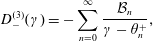 $$\begin{eqnarray}\displaystyle D_{-}^{(3)}(\unicode[STIX]{x1D6FE})=-\mathop{\sum }_{n=0}^{\infty }\frac{{\mathcal{B}}_{n}}{\unicode[STIX]{x1D6FE}-\unicode[STIX]{x1D703}_{n}^{+}}, & & \displaystyle\end{eqnarray}$$
 where  ${\mathcal{B}}_{n}$ are the residues of $D_{-}^{(2)}(\unicode[STIX]{x1D6FE}_{1})+D_{-}^{(4)}(\unicode[STIX]{x1D6FE}_{1})$ at $\unicode[STIX]{x1D6FE}=\unicode[STIX]{x1D703}_{n}^{+}$. The residues of $D_{-}^{(4)}$ are currently unknown, but the residues of $D_{-}^{(2)}$ are given by
 $$\begin{eqnarray}\displaystyle D_{r,k}^{(2)} & = & \displaystyle \frac{\text{e}^{2\text{i}\unicode[STIX]{x1D703}_{k}^{+}}}{K_{-}^{\prime }(\unicode[STIX]{x1D703}_{k}^{+})}\left\{\frac{-w_{0}(\unicode[STIX]{x1D714}-k_{x})\text{e}^{2\text{i}k_{x}/\unicode[STIX]{x1D6FD}^{2}}}{(2\unicode[STIX]{x03C0}\unicode[STIX]{x1D6FD})^{2}\text{i}(\unicode[STIX]{x1D703}_{k}^{+}+k_{x}/\unicode[STIX]{x1D6FD}^{2})(\unicode[STIX]{x1D703}_{k}^{+}+\unicode[STIX]{x1D714}/\unicode[STIX]{x1D6FD}^{2})K_{+}(-k_{x}/\unicode[STIX]{x1D6FD}^{2})}\right.\nonumber\\ \displaystyle & & \displaystyle +\left.\mathop{\sum }_{n=0}^{\infty }\frac{\text{i}{\mathcal{A}}_{n}\text{e}^{\text{i}(\unicode[STIX]{x1D703}_{k}^{+}-\unicode[STIX]{x1D703}_{n}^{-})}K_{-}(\unicode[STIX]{x1D703}_{n}^{-})}{(\unicode[STIX]{x1D703}_{k}^{+}+\unicode[STIX]{x1D714}/\unicode[STIX]{x1D6FD}^{2})(\unicode[STIX]{x1D703}_{k}^{+}-\unicode[STIX]{x1D703}_{n}^{-})}\right\}.\nonumber\end{eqnarray}$$
We may now substitute (A 30) into (A 28) to obtain the Wiener–Hopf equation
 $$\begin{eqnarray}\displaystyle \frac{F_{-}^{(3)}(\unicode[STIX]{x1D6FE})}{4\unicode[STIX]{x03C0}K_{-}(\unicode[STIX]{x1D6FE})}+\mathop{\sum }_{n=0}^{\infty }\frac{{\mathcal{B}}_{n}}{\unicode[STIX]{x1D6FE}-\unicode[STIX]{x1D703}_{n}^{+}}K_{+}(\unicode[STIX]{x1D703}_{n}^{+})=D_{+}^{(3)}(\unicode[STIX]{x1D6FE})K_{+}(\unicode[STIX]{x1D6FE})-\mathop{\sum }_{n=0}^{\infty }\frac{{\mathcal{B}}_{n}}{\unicode[STIX]{x1D6FE}-\unicode[STIX]{x1D703}_{n}^{+}}(K_{+}(\unicode[STIX]{x1D6FE})-K_{+}(\unicode[STIX]{x1D703}_{n}^{+})). & & \displaystyle \nonumber\end{eqnarray}$$
The edge conditions are identical to those applied in § A.1, and we employ the typical Wiener–Hopf argument to obtain
 $$\begin{eqnarray}\displaystyle D_{+}^{(3)}(\unicode[STIX]{x1D6FE})=\mathop{\sum }_{n=0}^{\infty }\frac{{\mathcal{B}}_{n}}{\unicode[STIX]{x1D6FE}-\unicode[STIX]{x1D703}_{n}^{+}}\left\{1-\frac{K_{+}(\unicode[STIX]{x1D703}_{n}^{+})}{K_{+}(\unicode[STIX]{x1D6FE})}\right\}. & & \displaystyle \nonumber\end{eqnarray}$$
Combining this solution with (A 30) yields
 $$\begin{eqnarray}\displaystyle D^{(3)}(\unicode[STIX]{x1D6FE})=-\mathop{\sum }_{n=0}^{\infty }\frac{{\mathcal{B}}_{n}}{\unicode[STIX]{x1D6FE}-\unicode[STIX]{x1D703}_{n}^{+}}\,\frac{K_{+}(\unicode[STIX]{x1D703}_{n}^{+})}{K_{+}(\unicode[STIX]{x1D6FE})}. & & \displaystyle\end{eqnarray}$$
 We proceed to the solution for  $D^{(4)}$. In a similar way to § A.2, we may invert the Fourier transform for the downstream boundary condition (A 7b) to write
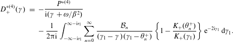 $$\begin{eqnarray}\displaystyle D_{+}^{\ast (4)}(\unicode[STIX]{x1D6FE}) & = & \displaystyle -\frac{P^{\ast (4)}}{\text{i}(\unicode[STIX]{x1D6FE}+\unicode[STIX]{x1D714}/\unicode[STIX]{x1D6FD}^{2})}\nonumber\\ \displaystyle & & \displaystyle -\,\frac{1}{2\unicode[STIX]{x03C0}\text{i}}\int _{-\infty -\text{i}\unicode[STIX]{x1D70F}_{1}}^{\infty -\text{i}\unicode[STIX]{x1D70F}_{1}}\mathop{\sum }_{n=0}^{\infty }\frac{{\mathcal{B}}_{n}}{(\unicode[STIX]{x1D6FE}_{1}-\unicode[STIX]{x1D6FE})(\unicode[STIX]{x1D6FE}_{1}-\unicode[STIX]{x1D703}_{n}^{+})}\left\{1-\frac{K_{+}(\unicode[STIX]{x1D703}_{n}^{+})}{K_{+}(\unicode[STIX]{x1D6FE}_{1})}\right\}\text{e}^{-2\text{i}\unicode[STIX]{x1D6FE}_{1}}\,\text{d}\unicode[STIX]{x1D6FE}_{1}.\nonumber\end{eqnarray}$$
 This integral can be closed in  ${\mathcal{L}}^{-}$ to obtain
 $$\begin{eqnarray}\displaystyle D_{+}^{\ast (4)}(\unicode[STIX]{x1D6FE})=-\frac{P^{\ast (4)}}{\unicode[STIX]{x1D6FE}+\unicode[STIX]{x1D714}/\unicode[STIX]{x1D6FD}^{2}}-\mathop{\sum }_{n=0}^{\infty }\frac{{\mathcal{C}}_{n}\text{e}^{-2\text{i}\unicode[STIX]{x1D703}_{n}^{-}}}{\text{i}(\unicode[STIX]{x1D703}_{n}^{-}+\unicode[STIX]{x1D714}/\unicode[STIX]{x1D6FD}^{2})(\unicode[STIX]{x1D6FE}-\unicode[STIX]{x1D703}_{n}^{-})}, & & \displaystyle\end{eqnarray}$$
where
 $$\begin{eqnarray}\displaystyle {\mathcal{C}}_{n}=\mathop{\sum }_{m=0}^{\infty }\frac{\text{i}(\unicode[STIX]{x1D703}_{n}^{-}+\unicode[STIX]{x1D714}/\unicode[STIX]{x1D6FD}^{2})}{(\unicode[STIX]{x1D703}_{m}^{+}-\unicode[STIX]{x1D703}_{n}^{-})}\,\frac{K_{+}(\unicode[STIX]{x1D703}_{m}^{+})}{K_{+}^{\prime }(\unicode[STIX]{x1D703}_{n}^{-})}\boldsymbol{\cdot }{\mathcal{B}}_{m}. & & \displaystyle \nonumber\end{eqnarray}$$
After truncation, we may write this system of equations in matrix form
 $$\begin{eqnarray}\displaystyle \boldsymbol{{\mathcal{C}}}=\unicode[STIX]{x1D647}\boldsymbol{{\mathcal{B}}}, & & \displaystyle\end{eqnarray}$$
where
 $$\begin{eqnarray}\displaystyle \{\unicode[STIX]{x1D647}\}_{n,m}=\frac{\text{i}(\unicode[STIX]{x1D703}_{n}^{-}+\unicode[STIX]{x1D714}/\unicode[STIX]{x1D6FD}^{2})}{(\unicode[STIX]{x1D703}_{m}^{+}-\unicode[STIX]{x1D703}_{n}^{-})}\,\frac{K_{+}(\unicode[STIX]{x1D703}_{m}^{+})}{K_{+}^{\prime }(\unicode[STIX]{x1D703}_{n}^{-})}. & & \displaystyle \nonumber\end{eqnarray}$$
By applying the notation introduced in (A 25), we may express the Wiener–Hopf equation (A 29) in the form
 $$\begin{eqnarray}\displaystyle & & \displaystyle \frac{F_{+}^{\ast (4)}(\unicode[STIX]{x1D6FE})}{4\unicode[STIX]{x03C0}K_{+}(\unicode[STIX]{x1D6FE})}+P^{\ast (4)}[\tilde{K}_{-}(\unicode[STIX]{x1D6FE},-\unicode[STIX]{x1D714}/\unicode[STIX]{x1D6FD}^{2})]_{+}+\mathop{\sum }_{n=0}^{\infty }\frac{[\tilde{K}_{-}(\unicode[STIX]{x1D6FE},\unicode[STIX]{x1D703}_{n}^{-})]_{+}}{\text{i}(\unicode[STIX]{x1D703}_{n}^{-}+\unicode[STIX]{x1D714}/\unicode[STIX]{x1D6FD}^{2})}{\mathcal{C}}_{n}\text{e}^{-2\text{i}\unicode[STIX]{x1D703}_{n}^{-}}\nonumber\\ \displaystyle & & \displaystyle \qquad =D_{-}^{\ast (4)}(\unicode[STIX]{x1D6FE})K_{-}(\unicode[STIX]{x1D6FE})-P^{\ast (4)}[\tilde{K}_{-}(\unicode[STIX]{x1D6FE},-\unicode[STIX]{x1D714}/\unicode[STIX]{x1D6FD}^{2})]_{-}-\mathop{\sum }_{n=0}^{\infty }\frac{[\tilde{K}_{-}(\unicode[STIX]{x1D6FE},\unicode[STIX]{x1D703}_{n}^{-})]_{-}}{\text{i}(\unicode[STIX]{x1D703}_{n}^{-}+\unicode[STIX]{x1D714}/\unicode[STIX]{x1D6FD}^{2})}{\mathcal{C}}_{n}\text{e}^{-2\text{i}\unicode[STIX]{x1D703}_{n}^{-}}.\quad \qquad\end{eqnarray}$$
Employing the unsteady Kutta condition in (A 34) yields
 $$\begin{eqnarray}\displaystyle P^{\ast (4)}=-\mathop{\sum }_{n=0}^{\infty }\frac{{\mathcal{C}}_{n}\text{e}^{-2\text{i}\unicode[STIX]{x1D703}_{n}^{-}}}{\text{i}(\unicode[STIX]{x1D703}_{n}^{-}+\unicode[STIX]{x1D714}/\unicode[STIX]{x1D6FD}^{2})}\,\frac{K_{-}(\unicode[STIX]{x1D703}_{n}^{-})}{K_{-}(-\unicode[STIX]{x1D714}/\unicode[STIX]{x1D6FD}^{2})}. & & \displaystyle \nonumber\end{eqnarray}$$
Finally, applying the downstream boundary condition (A 32) and rearranging (A 34) yields
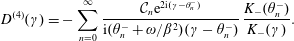 $$\begin{eqnarray}\displaystyle D^{(4)}(\unicode[STIX]{x1D6FE})=-\mathop{\sum }_{n=0}^{\infty }\frac{{\mathcal{C}}_{n}\text{e}^{2\text{i}(\unicode[STIX]{x1D6FE}-\unicode[STIX]{x1D703}_{n}^{-})}}{\text{i}(\unicode[STIX]{x1D703}_{n}^{-}+\unicode[STIX]{x1D714}/\unicode[STIX]{x1D6FD}^{2})(\unicode[STIX]{x1D6FE}-\unicode[STIX]{x1D703}_{n}^{-})}\,\frac{K_{-}(\unicode[STIX]{x1D703}_{n}^{-})}{K_{-}(\unicode[STIX]{x1D6FE})}. & & \displaystyle\end{eqnarray}$$
 We are now able to calculate the residues of  $D^{(3)}$ as
 $$\begin{eqnarray}\displaystyle {\mathcal{B}}_{n}=D_{r,n}^{(2)}-\mathop{\sum }_{m=0}^{\infty }\frac{{\mathcal{C}}_{n}\text{e}^{2\text{i}(\unicode[STIX]{x1D703}_{n}^{+}-\unicode[STIX]{x1D703}_{m}^{-})}}{\text{i}(\unicode[STIX]{x1D703}_{n}^{+}+\unicode[STIX]{x1D714}/\unicode[STIX]{x1D6FD}^{2})(\unicode[STIX]{x1D703}_{n}^{+}-\unicode[STIX]{x1D703}_{m}^{-})}\,\frac{K_{-}(\unicode[STIX]{x1D703}_{m}^{-})}{K_{-}^{\prime }(\unicode[STIX]{x1D703}_{n}^{+})}, & & \displaystyle \nonumber\end{eqnarray}$$
or, in matrix form,
 $$\begin{eqnarray}\displaystyle \boldsymbol{{\mathcal{B}}}=\boldsymbol{D}_{r}+\unicode[STIX]{x1D641}\boldsymbol{{\mathcal{C}}}, & & \displaystyle\end{eqnarray}$$
where
 $$\begin{eqnarray}\displaystyle \{\unicode[STIX]{x1D641}\}_{n,m}=\frac{\text{i}\text{e}^{2\text{i}(\unicode[STIX]{x1D703}_{n}^{+}-\unicode[STIX]{x1D703}_{m}^{-})}}{(\unicode[STIX]{x1D703}_{n}^{+}+\unicode[STIX]{x1D714}/\unicode[STIX]{x1D6FD}^{2})(\unicode[STIX]{x1D703}_{n}^{+}-\unicode[STIX]{x1D703}_{m}^{-})}\,\frac{K_{-}(\unicode[STIX]{x1D703}_{m}^{-})}{K_{-}^{\prime }(\unicode[STIX]{x1D703}_{n}^{+})}. & & \displaystyle \nonumber\end{eqnarray}$$
We can combine (A 33) and (A 36) to obtain
 $$\begin{eqnarray}\displaystyle (\unicode[STIX]{x1D644}-\unicode[STIX]{x1D641}\unicode[STIX]{x1D647})\boldsymbol{{\mathcal{B}}}=\boldsymbol{D}_{r}. & & \displaystyle\end{eqnarray}$$
 This matrix equation has important physical implications. If the matrix  $\unicode[STIX]{x1D644}-\unicode[STIX]{x1D641}\unicode[STIX]{x1D647}$ is not singular then it can be inverted to find $\boldsymbol{{\mathcal{B}}}$, and then $\boldsymbol{{\mathcal{C}}}$ by (A 33). On the other hand, if $\unicode[STIX]{x1D644}-\unicode[STIX]{x1D641}\unicode[STIX]{x1D647}$ is singular then there is no solution to the inhomogeneous linear system. However, in such a scenario there is a zero eigenvalue, so the homogeneous linear system ( $\boldsymbol{D}_{r}=\mathbf{0}$) has a non-trivial solution. Physically speaking, this means that at certain frequencies there exist non-trivial solutions for the scattering by an incident wave of zero amplitude. Such solutions correspond to the so-called ‘Parker modes’ discovered by Parker (Reference Parker1967), who observed resonance caused by the shedding frequency of the wake coinciding with the natural frequency of the cascade. Koch (Reference Koch1983) extended Parker’s results to calculate the resonant frequencies for staggered cascades in a mean flow by using a Wiener–Hopf approach much like the present work. Woodley & Peake (Reference Woodley and Peake1999) also deployed the Wiener–Hopf technique to calculate the resonant frequency of tandem cascades. While we do not investigate this further now, the present method could be used to investigate how surface treatments can be used to avoid resonance; the aforementioned references only considered case 0 cascades, whereas our approach can consider more general boundary conditions.
Appendix B. Factorisation of kernel function
The kernel function is defined as (A 12)
 $$\begin{eqnarray}\displaystyle K(\unicode[STIX]{x1D6FE})=\frac{K_{n}(\unicode[STIX]{x1D6FE})}{K_{d}(\unicode[STIX]{x1D6FE})}, & & \displaystyle\end{eqnarray}$$
where the numerator and denominator functions are respectively
 $$\begin{eqnarray}\displaystyle & \displaystyle K_{n}(\unicode[STIX]{x1D6FE})=\unicode[STIX]{x1D701}\sin (s\unicode[STIX]{x1D701})-(\unicode[STIX]{x1D707}_{0}-\text{i}\unicode[STIX]{x1D707}_{1}\unicode[STIX]{x1D6FE}-\unicode[STIX]{x1D707}_{2}\unicode[STIX]{x1D6FE}^{2})(\cos (s\unicode[STIX]{x1D701})-\cos (d\unicode[STIX]{x1D6FE}+\unicode[STIX]{x1D70E}^{\prime })), & \displaystyle\end{eqnarray}$$
 $$\begin{eqnarray}\displaystyle & \displaystyle K_{d}(\unicode[STIX]{x1D6FE})=4\unicode[STIX]{x03C0}(\cos (s\unicode[STIX]{x1D701})-\cos (d\unicode[STIX]{x1D6FE}+\unicode[STIX]{x1D70E}^{\prime })). & \displaystyle\end{eqnarray}$$
 Our goal is now to obtain a multiplicative factorisation of  $K$ into two parts that have no poles or zeros in ${\mathcal{L}}^{\pm }$ respectively. We restrict our attention to the upper half plane since a corresponding factorisation for the lower half plane can be constructed through symmetry.
B.1 Factorisation of poles of $K$

Previous work (Peake Reference Peake1992; Glegg Reference Glegg1999) has factorised the poles of  $K$ into the form
 $$\begin{eqnarray}\displaystyle K_{d}(\unicode[STIX]{x1D6FE})=K_{d}(0)\mathop{\prod }_{m=-\infty }^{\infty }\left(1-\frac{\unicode[STIX]{x1D6FE}}{\unicode[STIX]{x1D706}_{m}^{+}}\right)\left(1-\frac{\unicode[STIX]{x1D6FE}}{\unicode[STIX]{x1D706}_{m}^{-}}\right), & & \displaystyle \nonumber\end{eqnarray}$$
where
 $$\begin{eqnarray}\displaystyle \unicode[STIX]{x1D706}_{m}^{\pm }=-f_{m}\sin (\unicode[STIX]{x1D712})\pm \cos (\unicode[STIX]{x1D712})\unicode[STIX]{x1D701}(f_{m}),\quad f_{m}=\frac{\unicode[STIX]{x1D70E}^{\prime }-2\unicode[STIX]{x03C0}m}{\unicode[STIX]{x1D6E5}}. & & \displaystyle\end{eqnarray}$$
The asymptotic behaviour of these poles is
 $$\begin{eqnarray}\displaystyle & \displaystyle \unicode[STIX]{x1D706}_{m}^{+}\sim \unicode[STIX]{x1D706}_{R}^{(0)+}m+\unicode[STIX]{x1D706}_{R}^{(2)+}+o(1), & \displaystyle\end{eqnarray}$$
 $$\begin{eqnarray}\displaystyle & \displaystyle \unicode[STIX]{x1D706}_{-m}^{+}\sim \unicode[STIX]{x1D706}_{L}^{(0)+}m+\unicode[STIX]{x1D706}_{L}^{(2)+}+o(1), & \displaystyle\end{eqnarray}$$
 as  $m\rightarrow \infty$ where
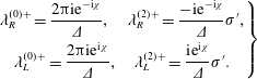 $$\begin{eqnarray}\left.\begin{array}{@{}c@{}}\displaystyle \unicode[STIX]{x1D706}_{R}^{(0)+}=\frac{2\unicode[STIX]{x03C0}\text{i}\text{e}^{-\text{i}\unicode[STIX]{x1D712}}}{\unicode[STIX]{x1D6E5}},\quad \unicode[STIX]{x1D706}_{R}^{(2)+}=\frac{-\text{i}\text{e}^{-\text{i}\unicode[STIX]{x1D712}}}{\unicode[STIX]{x1D6E5}}\unicode[STIX]{x1D70E}^{\prime },\\ \displaystyle \unicode[STIX]{x1D706}_{L}^{(0)+}=\frac{2\unicode[STIX]{x03C0}\text{i}\text{e}^{\text{i}\unicode[STIX]{x1D712}}}{\unicode[STIX]{x1D6E5}},\quad \unicode[STIX]{x1D706}_{L}^{(2)+}=\frac{\text{i}\text{e}^{\text{i}\unicode[STIX]{x1D712}}}{\unicode[STIX]{x1D6E5}}\unicode[STIX]{x1D70E}^{\prime }.\end{array}\right\}\end{eqnarray}$$
 The subscripts  $R$ and $L$ indicate that the pole is in the right or left side of ${\mathcal{L}}^{+}$ respectively.
B.2 Factorisation of zeros of $K$

We now outline the procedure for factorising the zeros of  $K_{n}$. In contrast to previous analyses for case 0 plates (Peake Reference Peake1992; Glegg Reference Glegg1999), no analytic expression for the zeros is available. In contrast, asymptotic expansions for the large zeros are still tractable, which is useful in two regards. First, the asymptotic expansions provide a good initial guess for a Newton solver to determine some of the actual roots. Second, the asymptotic expansions can be used to bound the growth of the factorised Wiener–Hopf kernel in ${\mathcal{L}}^{\pm }$. Understanding this growth is an important step in the Wiener–Hopf procedure, specifically the determination of the relevant entire function.
We focus on the zeros located in the first quadrant of the complex  $\unicode[STIX]{x1D6FE}$-plane. These roots are labelled as $\unicode[STIX]{x1D703}_{n,R}^{+}$. The asymptotic behaviour of the roots in the other quadrants can be determined by a similar procedure.
Recall the definition of the branch cut of  $\unicode[STIX]{x1D701}$
 $$\begin{eqnarray}\displaystyle \unicode[STIX]{x1D701}=\sqrt{\unicode[STIX]{x1D714}^{2}w^{2}-\unicode[STIX]{x1D6FE}^{2}}=\text{e}^{\text{i}\unicode[STIX]{x1D713}_{1}/2}\text{e}^{\text{i}\unicode[STIX]{x1D713}_{2}/2}|\unicode[STIX]{x1D714}^{2}w^{2}-\unicode[STIX]{x1D6FE}^{2}|^{1/2}, & & \displaystyle \nonumber\end{eqnarray}$$
where
 $$\begin{eqnarray}\displaystyle \unicode[STIX]{x1D713}_{1}=\arg (\unicode[STIX]{x1D714}w-\unicode[STIX]{x1D6FE}),\quad \unicode[STIX]{x1D713}_{2}=\arg (\unicode[STIX]{x1D714}w+\unicode[STIX]{x1D6FE}), & & \displaystyle \nonumber\end{eqnarray}$$
and
 $$\begin{eqnarray}\displaystyle \unicode[STIX]{x03C0}/2<\unicode[STIX]{x1D713}_{1}<5\unicode[STIX]{x03C0}/2,\quad -\unicode[STIX]{x03C0}/2<\unicode[STIX]{x1D713}_{2}<3\unicode[STIX]{x03C0}/2. & & \displaystyle \nonumber\end{eqnarray}$$
 Since the  $\unicode[STIX]{x1D703}_{n,R}^{+}$ are in the first quadrant, we have
 $$\begin{eqnarray}\displaystyle \unicode[STIX]{x1D701}(\unicode[STIX]{x1D703}_{n,R}^{+})\sim \text{i}\unicode[STIX]{x1D703}_{n,R}^{+},\quad \text{as }n\rightarrow \infty . & & \displaystyle \nonumber\end{eqnarray}$$
This leads us to determine the following asymptotic behaviours:
 $$\begin{eqnarray}\displaystyle & \displaystyle \sin (s\unicode[STIX]{x1D701}(\unicode[STIX]{x1D703}_{n,R}^{+}))\sim -\frac{1}{2\text{i}}\text{e}^{s\unicode[STIX]{x1D703}_{n,R}^{+}}, & \displaystyle \nonumber\\ \displaystyle & \displaystyle \cos (s\unicode[STIX]{x1D701}(\unicode[STIX]{x1D703}_{n,R}^{+}))\sim {\textstyle \frac{1}{2}}\text{e}^{s\unicode[STIX]{x1D703}_{n,R}^{+}},\quad \cos (d\unicode[STIX]{x1D703}_{n,R}^{+}+\unicode[STIX]{x1D70E}^{\prime })\sim {\textstyle \frac{1}{2}}\text{e}^{-\text{i}(d\unicode[STIX]{x1D703}_{n,R}^{+}+\unicode[STIX]{x1D70E}^{\prime })}. & \displaystyle \nonumber\end{eqnarray}$$
 We now substitute these representations into (B 1) to obtain asymptotic expansions for the roots  $\unicode[STIX]{x1D703}_{n,R}^{+}$. Each case must be considered separately, although the asymptotic behaviours are similar.
Case I boundary condition
For the no-mean-flow boundary condition, the asymptotic behaviour of the roots obeys
 $$\begin{eqnarray}\displaystyle \unicode[STIX]{x1D703}_{n,R}^{+}\sim -\unicode[STIX]{x1D707}_{0}(1-\exp [-\text{i}((d-\text{i}s)\unicode[STIX]{x1D703}_{n,R}^{+}+\unicode[STIX]{x1D70E}^{\prime })]). & & \displaystyle\end{eqnarray}$$
We seek an asymptotic expansion of the first quadrant roots of the classical form
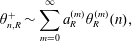 $$\begin{eqnarray}\displaystyle \unicode[STIX]{x1D703}_{n,R}^{+}\sim \mathop{\sum }_{m=0}^{\infty }a_{R}^{(m)}\unicode[STIX]{x1D703}_{R}^{(m)}(n), & & \displaystyle\end{eqnarray}$$
 where  $\unicode[STIX]{x1D703}_{R}^{(m+1)}(n)=o(\unicode[STIX]{x1D703}_{R}^{(m)}(n))$ as $n\rightarrow \infty$. In (B 8) we require the linear (left) and exponential (right) terms to match. However, since $|\unicode[STIX]{x1D703}_{n,R}^{+}|\rightarrow \infty$ as $n\rightarrow \infty$, the exponential term will generally grow at a faster rate than the linear term. Consequently, the real part of the argument of the exponential must be asymptotically small compared to the imaginary part. We therefore expand the roots into real and imaginary parts as $\unicode[STIX]{x1D703}_{n,R}^{+}=\unicode[STIX]{x1D703}_{n,R}^{r+}+\text{i}\unicode[STIX]{x1D703}_{n,R}^{i+}$ and write
 $$\begin{eqnarray}\displaystyle d\unicode[STIX]{x1D703}_{n,R}^{i+}-s\unicode[STIX]{x1D703}_{n,R}^{r+}=G(n), & & \displaystyle\end{eqnarray}$$
 where  $G(n)=o(\unicode[STIX]{x1D703}_{R}^{(0)}(n))$. Rearranging yields
 $$\begin{eqnarray}\displaystyle \unicode[STIX]{x1D703}_{n,R}^{+}=\unicode[STIX]{x1D703}_{n,R}^{+}+\text{i}\unicode[STIX]{x1D703}_{n,R}^{i+}=\left(1+\text{i}\frac{s}{d}\right)\unicode[STIX]{x1D703}_{n,R}^{r+}+\text{i}\frac{G(n)}{d}. & & \displaystyle \nonumber\end{eqnarray}$$
Since the arguments of the left- and right-hand sides of (B 8) must match, we obtain an expression for the imaginary part of the argument of the exponential:
 $$\begin{eqnarray}\displaystyle \unicode[STIX]{x1D70E}^{\prime }+d\unicode[STIX]{x1D703}_{n,R}^{r+}+s\unicode[STIX]{x1D703}_{n,R}^{i+}=\unicode[STIX]{x1D712}-2n\unicode[STIX]{x03C0}+o(1). & & \displaystyle\end{eqnarray}$$
Applying the asymptotic expansion (B 9) and taking the leading-order terms of (B 10) and (B 11) yields
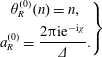 $$\begin{eqnarray}\displaystyle \left.\begin{array}{@{}c@{}}\displaystyle \unicode[STIX]{x1D703}_{R}^{(0)}(n)=n,\\ \displaystyle a_{R}^{(0)}=\frac{2\unicode[STIX]{x03C0}\text{i}\text{e}^{-\text{i}\unicode[STIX]{x1D712}}}{\unicode[STIX]{x1D6E5}}.\end{array}\right\} & & \displaystyle\end{eqnarray}$$
 We may now substitute the expansion for  $\unicode[STIX]{x1D703}_{n,R}^{+}$ so far into (B 8) to obtain
 $$\begin{eqnarray}\displaystyle \frac{2\unicode[STIX]{x03C0}\text{i}\text{e}^{-\text{i}\unicode[STIX]{x1D712}}}{\unicode[STIX]{x1D6E5}}n+o(n)\sim -\unicode[STIX]{x1D707}_{0}(1-\exp [G(n)-\text{i}\unicode[STIX]{x1D712}]). & & \displaystyle \nonumber\end{eqnarray}$$
We now match leading-order terms to obtain
 $$\begin{eqnarray}\displaystyle \frac{2\unicode[STIX]{x03C0}}{\unicode[STIX]{x1D6E5}}n=-\unicode[STIX]{x1D707}_{0}\exp [G(n)], & & \displaystyle \nonumber\end{eqnarray}$$
so that
 $$\begin{eqnarray}\displaystyle G(n)=\log (n)+\log \left(\frac{-2\unicode[STIX]{x03C0}}{\unicode[STIX]{x1D707}_{0}\unicode[STIX]{x1D6E5}}\right). & & \displaystyle \nonumber\end{eqnarray}$$
Similarly, taking the leading-order terms in (B 10) and (B 11) yields
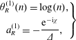 $$\begin{eqnarray}\displaystyle \left.\begin{array}{@{}c@{}}\displaystyle \unicode[STIX]{x1D703}_{R}^{(1)}(n)=\log (n),\\ \displaystyle a_{R}^{(1)}=-\frac{\text{e}^{-\text{i}\unicode[STIX]{x1D712}}}{\unicode[STIX]{x1D6E5}},\end{array}\right\} & & \displaystyle\end{eqnarray}$$
and
 $$\begin{eqnarray}\displaystyle \left.\begin{array}{@{}c@{}}\displaystyle \unicode[STIX]{x1D703}_{R}^{(2)}(n)=1,\\ \displaystyle a_{R}^{(2)}=\frac{\text{i}\text{e}^{-\text{i}\unicode[STIX]{x1D712}}}{\unicode[STIX]{x1D6E5}}\left(\frac{\unicode[STIX]{x03C0}}{2}+\unicode[STIX]{x1D712}+\text{i}\log \left(\frac{-2\unicode[STIX]{x03C0}}{\unicode[STIX]{x1D707}_{0}\unicode[STIX]{x1D6E5}}\right)-\unicode[STIX]{x1D70E}^{\prime }\right).\end{array}\right\} & & \displaystyle\end{eqnarray}$$
Substitution of ((B 12), (B 13), (B 14)) into the asymptotic expansion (B 9) yields
 $$\begin{eqnarray}\displaystyle \unicode[STIX]{x1D703}_{n,R}^{+}\sim \frac{\text{e}^{-\text{i}\unicode[STIX]{x1D712}}}{\unicode[STIX]{x1D6E5}}\left(2\unicode[STIX]{x03C0}\text{i}n-\log (n)+\text{i}\left(\frac{\unicode[STIX]{x03C0}}{2}+\unicode[STIX]{x1D712}-\unicode[STIX]{x1D70E}^{\prime }\right)-\log \left(\frac{-2\unicode[STIX]{x03C0}}{\unicode[STIX]{x1D707}_{0}\unicode[STIX]{x1D6E5}}\right)+o(1)\right). & & \displaystyle\end{eqnarray}$$
Similar analysis yields the asymptotic behaviour for the roots in the second quadrant as
 $$\begin{eqnarray}\displaystyle \unicode[STIX]{x1D703}_{n,L}^{+}\sim \frac{\text{e}^{\text{i}\unicode[STIX]{x1D712}}}{\unicode[STIX]{x1D6E5}}\left(2\unicode[STIX]{x03C0}\text{i}n+\log (n)+\text{i}\left(\frac{\unicode[STIX]{x03C0}}{2}+\unicode[STIX]{x1D712}+\unicode[STIX]{x1D70E}^{\prime }\right)+\log \left(\frac{-2\unicode[STIX]{x03C0}}{\unicode[STIX]{x1D707}_{0}\unicode[STIX]{x1D6E5}}\right)+o(1)\right). & & \displaystyle\end{eqnarray}$$
Case II boundary condition
In the case of a porous blade in a background flow, the asymptotic behaviour of the roots obeys the equation
 $$\begin{eqnarray}\displaystyle 1\sim \text{i}\unicode[STIX]{x1D707}_{1}(1-\exp [-\text{i}((d-\text{i}s)\unicode[STIX]{x1D703}_{n,R}^{+}+\unicode[STIX]{x1D70E}^{\prime })]). & & \displaystyle\end{eqnarray}$$
We assume an asymptotic expansion of the roots of the form (B 9). Similar reasoning to the previous section yields that the leading-order terms are also given by
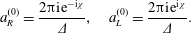 $$\begin{eqnarray}\displaystyle a_{R}^{(0)}=\frac{2\unicode[STIX]{x03C0}\text{i}\text{e}^{-\text{i}\unicode[STIX]{x1D712}}}{\unicode[STIX]{x1D6E5}},\quad a_{L}^{(0)}=\frac{2\unicode[STIX]{x03C0}\text{i}\text{e}^{\text{i}\unicode[STIX]{x1D712}}}{\unicode[STIX]{x1D6E5}}. & & \displaystyle\end{eqnarray}$$
We may now solve (B 17) directly to find the coefficients of the next two orders of the asymptotic expansion as
 $$\begin{eqnarray}\displaystyle & \displaystyle a_{R}^{(1)}=0,\quad a_{L}^{(1)}=0, & \displaystyle \nonumber\\ \displaystyle & \displaystyle a_{R}^{(2)}=-\frac{\text{e}^{-\text{i}\unicode[STIX]{x1D712}}}{\unicode[STIX]{x1D6E5}}\left(\log \left(1+\frac{\text{i}}{\unicode[STIX]{x1D707}_{0}}\right)+\text{i}\unicode[STIX]{x1D70E}^{\prime }\right),\quad a_{L}^{(2)}=\frac{\text{e}^{\text{i}\unicode[STIX]{x1D712}}}{\unicode[STIX]{x1D6E5}}\left(\log \left(1-\frac{\text{i}}{\unicode[STIX]{x1D707}_{0}}\right)+\text{i}\unicode[STIX]{x1D70E}^{\prime }\right). & \displaystyle \nonumber\end{eqnarray}$$
Case III boundary condition
For the case III boundary condition, the asymptotic behaviour of the roots obeys
 $$\begin{eqnarray}\displaystyle 1\sim \unicode[STIX]{x1D707}_{2}\unicode[STIX]{x1D703}_{n,R}^{+}(1-\exp [-\text{i}((d-\text{i}s)\unicode[STIX]{x1D703}_{n,R}^{+}+\unicode[STIX]{x1D70E}^{\prime })]). & & \displaystyle\end{eqnarray}$$
Similar analysis to the previous sections possesses an identical asymptotic expansion (up to the terms considered) and we have, at leading order,
 $$\begin{eqnarray}\displaystyle a_{R}^{(0)}=\frac{2\unicode[STIX]{x03C0}\text{i}\text{e}^{-\text{i}\unicode[STIX]{x1D712}}}{\unicode[STIX]{x1D6E5}},\quad a_{L}^{(0)}=\frac{2\unicode[STIX]{x03C0}\text{i}\text{e}^{\text{i}\unicode[STIX]{x1D712}}}{\unicode[STIX]{x1D6E5}}. & & \displaystyle\end{eqnarray}$$
Substitution of (B 20) into (B 19) yields the coefficients of the next two orders of the asymptotic expansion as
 $$\begin{eqnarray}\displaystyle & \displaystyle a_{R}^{(1)}=0,\quad a_{L}^{(1)}=0, & \displaystyle \nonumber\\ \displaystyle & \displaystyle a_{R}^{(2)}=-\frac{\text{i}\unicode[STIX]{x1D70E}^{\prime }\text{e}^{-\text{i}\unicode[STIX]{x1D712}}}{\unicode[STIX]{x1D6E5}},\quad a_{L}^{(2)}=\frac{\text{i}\unicode[STIX]{x1D70E}^{\prime }\text{e}^{\text{i}\unicode[STIX]{x1D712}}}{\unicode[STIX]{x1D6E5}}. & \displaystyle \nonumber\end{eqnarray}$$
B.3 Full factorisation of kernel, $K$

We propose a multiplicative splitting of  $K$ of the form:
 $$\begin{eqnarray}\displaystyle K(\unicode[STIX]{x1D6FE})=K_{+}(\unicode[STIX]{x1D6FE})K_{-}(\unicode[STIX]{x1D6FE}), & & \displaystyle \nonumber\end{eqnarray}$$
where
 $$\begin{eqnarray}\displaystyle & \displaystyle K_{-}(\unicode[STIX]{x1D6FE})=\text{e}^{E(\unicode[STIX]{x1D6FE})}\frac{\displaystyle \mathop{\prod }_{m=1}^{\infty }(1-\unicode[STIX]{x1D6FE}/\unicode[STIX]{x1D703}_{m,R}^{+})(1-\unicode[STIX]{x1D6FE}/\unicode[STIX]{x1D703}_{m,L}^{+})}{\displaystyle \mathop{\prod }_{m=-\infty }^{\infty }(1-\unicode[STIX]{x1D6FE}/\unicode[STIX]{x1D706}_{m}^{+})}, & \displaystyle\end{eqnarray}$$
 $$\begin{eqnarray}\displaystyle & \displaystyle K_{+}(\unicode[STIX]{x1D6FE})=\text{e}^{-E(\unicode[STIX]{x1D6FE})}\frac{\displaystyle \mathop{\prod }_{m=1}^{\infty }(1-\unicode[STIX]{x1D6FE}/\unicode[STIX]{x1D703}_{m,R}^{-})(1-\unicode[STIX]{x1D6FE}/\unicode[STIX]{x1D703}_{m,L}^{-})}{\displaystyle \mathop{\prod }_{m=-\infty }^{\infty }(1-\unicode[STIX]{x1D6FE}/\unicode[STIX]{x1D706}_{m}^{-})}K(0). & \displaystyle\end{eqnarray}$$ $E$ is included to ensure that $K_{\pm }$ has algebraic growth in ${\mathcal{L}}^{\pm }$ respectively. Previous works for case 0 (Peake Reference Peake1992; Glegg Reference Glegg1999) have derived the form of the entire function $E$ and shown that it is a polynomial. In the remainder of this section, we will show that $E$ vanishes for cases I, II and III.
Asymptotic behaviour of proposed factorisation
We focus on  $K_{-}$ since the asymptotic behaviour of $K_{+}$ follows in an analogous manner. We first note that the infinite product
 $$\begin{eqnarray}\displaystyle P_{1}=\mathop{\prod }_{m=1}^{\infty }\left(\frac{a_{R}^{(0)}m+a_{R}^{(2)}}{\unicode[STIX]{x1D703}_{m,R}^{+}}\right)\left(\frac{a_{L}^{(0)}m+a_{L}^{(2)}}{\unicode[STIX]{x1D703}_{m,L}^{+}}\right) & & \displaystyle\end{eqnarray}$$
exists. This is seen by employing the asymptotic expansions (B 15) and (B 16) to obtain
 $$\begin{eqnarray}\displaystyle & \displaystyle \frac{a_{R}^{(0)}m+a_{R}^{(1)}}{\unicode[STIX]{x1D703}_{m,R}^{+}}=1-\frac{a_{R}^{(1)}\log (m)}{a_{R}^{(0)}m}+o(m^{-1}), & \displaystyle \nonumber\\ \displaystyle & \displaystyle \frac{a_{L}^{(0)}m+a_{L}^{(1)}}{\unicode[STIX]{x1D703}_{m,L}^{+}}=1-\frac{a_{L}^{(1)}\log (m)}{a_{L}^{(0)}m}+o(m^{-1}), & \displaystyle \nonumber\end{eqnarray}$$
respectively. Substitution into the product (B 22) yields
 $$\begin{eqnarray}\displaystyle P_{1}=\mathop{\prod }_{m=1}^{\infty }\left(1-R\frac{\log (m)}{m}+o(m^{-1})\right), & & \displaystyle\end{eqnarray}$$
where
 $$\begin{eqnarray}\displaystyle R=\frac{a_{R}^{(1)}}{a_{R}^{(0)}}+\frac{a_{L}^{(1)}}{a_{L}^{(0)}}=0, & & \displaystyle\end{eqnarray}$$
and the last identity is due to (B 12) and (B 13). Consequently, the products (B 23) and (B 22) exist via the comparison method. Moreover, we note that since
 $$\begin{eqnarray}\displaystyle & \displaystyle \text{Im}[a_{R}^{(0)}m_{1}+a_{R}^{(2)}-\unicode[STIX]{x1D6FE}]>m_{1}\text{Im}[a_{R}^{(0)}], & \displaystyle \nonumber\\ \displaystyle & \displaystyle \text{Im}[a_{L}^{(0)}m_{1}+a_{L}^{(2)}-\unicode[STIX]{x1D6FE}]>m_{1}\text{Im}[a_{L}^{(0)}], & \displaystyle \nonumber\end{eqnarray}$$
we can show that the infinite product
 $$\begin{eqnarray}\displaystyle P_{2}(\unicode[STIX]{x1D6FE})=\mathop{\prod }_{m=1}^{\infty }\left(\frac{\unicode[STIX]{x1D703}_{m,R}^{+}-\unicode[STIX]{x1D6FE}}{a_{R}^{(0)}m+a_{R}^{(2)}-\unicode[STIX]{x1D6FE}}\right)\left(\frac{\unicode[STIX]{x1D703}_{m,L}^{+}-\unicode[STIX]{x1D6FE}}{a_{L}^{(0)}m+a_{L}^{(2)}-\unicode[STIX]{x1D6FE}}\right) & & \displaystyle\end{eqnarray}$$
 has, at worst, algebraic growth as  $\unicode[STIX]{x1D6FE}\rightarrow \infty$ in ${\mathcal{L}}^{-}$, i.e. $\exists \unicode[STIX]{x1D6FC}$ s.t. $P(\unicode[STIX]{x1D6FE})\sim \unicode[STIX]{x1D6FE}^{\unicode[STIX]{x1D6FC}}$, up to a multiplicative constant. We now use $P_{1}$ and $P_{2}$ to calculate the asymptotic behaviour of $K_{-}$ by comparison with the product
 $$\begin{eqnarray}\displaystyle P(\unicode[STIX]{x1D6FE})=\mathop{\prod }_{m=1}^{\infty }{\displaystyle \frac{(1-\unicode[STIX]{x1D6FE}/\unicode[STIX]{x1D703}_{m,R}^{+})\text{e}^{\unicode[STIX]{x1D6FE}/\unicode[STIX]{x1D703}_{m,R}^{+}}(1-\unicode[STIX]{x1D6FE}/\unicode[STIX]{x1D703}_{m,L}^{+})\text{e}^{\unicode[STIX]{x1D6FE}/\unicode[STIX]{x1D703}_{m,L}^{+}}}{(1-\unicode[STIX]{x1D6FE}/(a_{R}^{(0)}m+a_{R}^{(2)}))\text{e}^{\unicode[STIX]{x1D6FE}/a_{R}^{(0)}m}(1-\unicode[STIX]{x1D6FE}/(a_{L}^{(0)}m+a_{L}^{(2)}))\text{e}^{\unicode[STIX]{x1D6FE}/a_{L}^{(0)}m}}}. & & \displaystyle\end{eqnarray}$$
This function may alternatively be written as
 $$\begin{eqnarray}\displaystyle P(\unicode[STIX]{x1D6FE})=\exp \left(\unicode[STIX]{x1D6FE}\mathop{\sum }_{m=1}^{\infty }\frac{1}{\unicode[STIX]{x1D703}_{m,R}^{+}}-\frac{1}{a_{R}^{(0)}m}+\frac{1}{\unicode[STIX]{x1D703}_{m,L}^{+}}-\frac{1}{a_{L}^{(0)}m}\right)P_{1}P_{2}(\unicode[STIX]{x1D6FE}). & & \displaystyle \nonumber\end{eqnarray}$$
 Since  $P_{1}$ exists and $P_{2}$ has algebraic growth as $\unicode[STIX]{x1D6FE}\rightarrow$ in ${\mathcal{L}}^{-}$, we have, up to a multiplication constant,
 $$\begin{eqnarray}\displaystyle P(\unicode[STIX]{x1D6FE})\sim P_{1}\unicode[STIX]{x1D6FE}^{\unicode[STIX]{x1D6FC}}\exp \left(\unicode[STIX]{x1D6FE}\mathop{\sum }_{m=1}^{\infty }\frac{1}{\unicode[STIX]{x1D703}_{m,R}^{+}}-\frac{1}{a_{R}^{(0)}m}+\frac{1}{\unicode[STIX]{x1D703}_{m,L}^{+}}-\frac{1}{a_{L}^{(0)}m}\right). & & \displaystyle \nonumber\end{eqnarray}$$
 We now calculate the growth of the denominators of  $P$. By applying the asymptotic behaviour of the gamma function (Peake Reference Peake1992, B7 & B8), we derive the relation
 $$\begin{eqnarray}\displaystyle \mathop{\prod }_{m=1}^{\infty }\left(1-\frac{\unicode[STIX]{x1D6FE}}{am+b}\right)\exp \left[\frac{\unicode[STIX]{x1D6FE}}{am}\right]\sim C\exp \left[\frac{\unicode[STIX]{x1D6FE}}{a}({\mathcal{E}}-1-\log (-a))+\left(\frac{\unicode[STIX]{x1D6FE}}{a}-\frac{b}{a}-\frac{1}{2}\right)\log (\unicode[STIX]{x1D6FE})\right]\!, & & \displaystyle \nonumber\end{eqnarray}$$
 where  ${\mathcal{E}}$ is the Euler–Mascheroni constant and
 $$\begin{eqnarray}\displaystyle C=\frac{-b}{\sqrt{2\unicode[STIX]{x03C0}}}\unicode[STIX]{x1D6E4}\left({\displaystyle \frac{b}{a}}\right)\left(-a\right)^{((b/a)-1/2)}. & & \displaystyle \nonumber\end{eqnarray}$$
This representation may be substituted into the denominator of (B 26). Rearranging yields the asymptotic behaviour
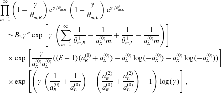 $$\begin{eqnarray}\displaystyle & & \displaystyle \mathop{\prod }_{m=1}^{\infty }\left(1-\frac{\unicode[STIX]{x1D6FE}}{\unicode[STIX]{x1D703}_{m,R}^{+}}\right)\text{e}^{\unicode[STIX]{x1D6FE}/\unicode[STIX]{x1D703}_{m,R}^{+}}\left(1-\frac{\unicode[STIX]{x1D6FE}}{\unicode[STIX]{x1D703}_{m,L}^{+}}\right)\text{e}^{\unicode[STIX]{x1D6FE}/\unicode[STIX]{x1D703}_{m,L}^{+}}\nonumber\\ \displaystyle & & \displaystyle \quad \sim B_{2}\unicode[STIX]{x1D6FE}^{\unicode[STIX]{x1D6FC}}\exp \left[\unicode[STIX]{x1D6FE}\left(\mathop{\sum }_{m=1}^{\infty }\frac{1}{\unicode[STIX]{x1D703}_{m,R}^{+}}-\frac{1}{a_{R}^{(0)}m}+\frac{1}{\unicode[STIX]{x1D703}_{m,L}^{+}}-\frac{1}{a_{L}^{(0)}m}\right)\right]\nonumber\\ \displaystyle & & \displaystyle \quad \times \exp \left[\frac{\unicode[STIX]{x1D6FE}}{a_{R}^{(0)}a_{L}^{(0)}}(({\mathcal{E}}-1)(a_{R}^{(0)}+a_{L}^{(0)})-a_{L}^{(0)}\log (-a_{R}^{(0)})-a_{R}^{(0)}\log (-a_{L}^{(0)}))\right]\nonumber\\ \displaystyle & & \displaystyle \quad \times \exp \left[\left(\unicode[STIX]{x1D6FE}\left(\frac{1}{a_{R}^{(0)}}+\frac{1}{a_{L}^{(0)}}\right)-\left(\frac{a_{R}^{(2)}}{a_{R}^{(0)}}+\frac{a_{L}^{(2)}}{a_{L}^{(0)}}\right)-1\right)\log (\unicode[STIX]{x1D6FE})\right],\nonumber\end{eqnarray}$$
 for some constant  $B_{2}$. We also note that
 $$\begin{eqnarray}\displaystyle & & \displaystyle \mathop{\prod }_{m=-\infty }^{\infty }\left(1-\frac{\unicode[STIX]{x1D6FE}}{\unicode[STIX]{x1D706}_{m}^{+}}\right)\text{e}^{\unicode[STIX]{x1D6FE}/\unicode[STIX]{x1D706}_{m}^{+}}\sim B_{3}\left(1-\frac{\unicode[STIX]{x1D6FE}}{\unicode[STIX]{x1D706}_{m}^{+}}\right)\exp \left[\unicode[STIX]{x1D6FE}\left(\frac{1}{\unicode[STIX]{x1D706}_{0}^{+}}+\mathop{\sum }_{\substack{ m=-\infty \\ m\neq 0}}^{\infty }\frac{1}{\unicode[STIX]{x1D706}_{m}^{+}}-\frac{1}{\unicode[STIX]{x1D706}_{R}^{(0)+}|m|}\right)\right]\nonumber\\ \displaystyle & & \displaystyle \quad \times \exp \left[\frac{\unicode[STIX]{x1D6FE}}{\unicode[STIX]{x1D706}_{R}^{(0)+}\unicode[STIX]{x1D706}_{L}^{(0)+}}(({\mathcal{E}}-1)(\unicode[STIX]{x1D706}_{R}^{(0)+}+\unicode[STIX]{x1D706}_{L}^{(0)+})-\unicode[STIX]{x1D706}_{L}^{(0)+}\log (-\unicode[STIX]{x1D706}_{R}^{(0)+})-\unicode[STIX]{x1D706}_{R}^{(0)+}\log (-\unicode[STIX]{x1D706}_{L}^{(0)+}))\right]\nonumber\\ \displaystyle & & \displaystyle \quad \times \exp \left[\left(\unicode[STIX]{x1D6FE}\left(\frac{1}{\unicode[STIX]{x1D706}_{R}^{(0)+}}+\frac{1}{\unicode[STIX]{x1D706}_{L}^{(0)+}}\right)-\left(\frac{\unicode[STIX]{x1D706}_{R}^{(2)+}}{\unicode[STIX]{x1D706}_{R}^{(0)+}}+\frac{\unicode[STIX]{x1D706}_{L}^{(2)+}}{\unicode[STIX]{x1D706}_{L}^{(0)+}}\right)-1\right)\log (\unicode[STIX]{x1D6FE})\right],\nonumber\end{eqnarray}$$
 for some constant  $B_{3}$. Noting that $\unicode[STIX]{x1D706}_{R}^{(0)+}=a_{R}^{(0)}$ and $\unicode[STIX]{x1D706}_{L}^{(0)+}=a_{L}^{(0)}$, and using (B 7), we obtain
 $$\begin{eqnarray}\displaystyle \frac{\displaystyle \mathop{\prod }_{m=1}^{\infty }(1-\unicode[STIX]{x1D6FE}/\unicode[STIX]{x1D703}_{m,R}^{+})(1-\unicode[STIX]{x1D6FE}/\unicode[STIX]{x1D703}_{m,L}^{+})}{\displaystyle \mathop{\prod }_{m=-\infty }^{\infty }(1-\unicode[STIX]{x1D6FE}/\unicode[STIX]{x1D706}_{m}^{+})}\sim B_{4}\unicode[STIX]{x1D6FE}^{c}, & & \displaystyle \nonumber\end{eqnarray}$$
 for some constant  $B_{4}$ and
 $$\begin{eqnarray}\displaystyle c=\unicode[STIX]{x1D6FC}-\left(\frac{a_{R}^{(2)}}{a_{R}^{(0)}}+\frac{a_{L}^{(2)}}{a_{L}^{(0)}}\right). & & \displaystyle \nonumber\end{eqnarray}$$
In particular, on a correct selection of the logarithmic branches, we find the following behaviours of the asymptotic factorisations of the kernels (subject to a multiplicative constant):
(i) Case 0,
$$\begin{eqnarray}\displaystyle K_{\pm }(\unicode[STIX]{x1D6FE})\sim \unicode[STIX]{x1D6FE}^{1/2}; & & \displaystyle \nonumber\end{eqnarray}$$(ii) Case I,
$$\begin{eqnarray}\displaystyle K_{\pm }(\unicode[STIX]{x1D6FE})\sim \unicode[STIX]{x1D6FE}^{1/2}; & & \displaystyle \nonumber\end{eqnarray}$$(iii) Case II,
for some non-negative integer$$\begin{eqnarray}\displaystyle K_{\pm }(\unicode[STIX]{x1D6FE})\sim \unicode[STIX]{x1D6FE}^{\mp (1/\unicode[STIX]{x03C0})\cot ^{-1}(\unicode[STIX]{x1D707}_{1})+n} & & \displaystyle \nonumber\end{eqnarray}$$$n$. It is worth noting that the above exponent has appeared before in the porous aerofoil literature. Baddoo, Hajian & Jaworski (Reference Baddoo, Hajian and Jaworski2019) showed that an incompressible, irrotational velocity field near a porous edge must scale like $\pm (1/\unicode[STIX]{x03C0})\cot ^{-1}(\unicode[STIX]{x1D713})+n$, where $\unicode[STIX]{x1D713}$ is the porosity parameter. It is not a coincidence that this factor also appears here: through the Wiener–Hopf analysis, the behaviour of the unsteady velocity field at the endpoints of the blade is governed by the behaviour of the factorised kernel at large $\unicode[STIX]{x1D6FE}$. Since the edge is self-similar, the singular behaviour is identical for the Laplace and Helmholtz equations.(iv) Case III:
$$\begin{eqnarray}\displaystyle K_{\pm }(\unicode[STIX]{x1D6FE})\sim \unicode[STIX]{x1D6FE}. & & \displaystyle \nonumber\end{eqnarray}$$


Appendix C. Details of Fourier inversion
The acoustic field is given by
 $$\begin{eqnarray}\displaystyle \unicode[STIX]{x1D719}(x,y)=\int _{-\infty }^{\infty }D(\unicode[STIX]{x1D6FE})A(x,y;\unicode[STIX]{x1D6FE})\,\text{d}\unicode[STIX]{x1D6FE}, & & \displaystyle \nonumber\end{eqnarray}$$
 where  $A=A_{u}+A_{d}$ and
 $$\begin{eqnarray}\displaystyle & \displaystyle A_{u}(x,y;\unicode[STIX]{x1D6FE})=-2\unicode[STIX]{x03C0}\frac{\text{e}^{\text{i}(d\unicode[STIX]{x1D6FE}+\unicode[STIX]{x1D70E}^{\prime })}\cos (\unicode[STIX]{x1D701}y)}{K_{d}(\unicode[STIX]{x1D6FE})}\text{e}^{-\text{i}\unicode[STIX]{x1D6FE}x}, & \displaystyle \nonumber\\ \displaystyle & \displaystyle A_{d}(x,y;\unicode[STIX]{x1D6FE})=2\unicode[STIX]{x03C0}\frac{\cos (\unicode[STIX]{x1D701}(y-s))}{K_{d}(\unicode[STIX]{x1D6FE})}\text{e}^{-\text{i}\unicode[STIX]{x1D6FE}x} & \displaystyle \nonumber\end{eqnarray}$$
 and  $K_{d}$ is the denominator of $K$ as defined in (B 3). We calculate the above integral by splitting the physical plane into five separate regions, as illustrated in figure 5. Both $A_{u}$ and $A_{d}$ have poles at the acoustic modes $\unicode[STIX]{x1D6FE}=\unicode[STIX]{x1D706}_{m}^{\pm }$ (B 4) which are the zeros of $K_{d}$. The residues at these points are
 $$\begin{eqnarray}\displaystyle & \displaystyle A_{u}^{r}(x,y;\unicode[STIX]{x1D706}_{m}^{\pm })=\mp \frac{\unicode[STIX]{x1D701}_{m}^{\pm }\text{e}^{\pm \text{i}s\unicode[STIX]{x1D701}_{m}^{\pm }}\cos (\unicode[STIX]{x1D701}_{m}^{\pm }y)}{2\unicode[STIX]{x1D6E5}\sin (s\unicode[STIX]{x1D701}_{m}^{\pm })\sqrt{\unicode[STIX]{x1D714}^{2}w^{2}-f_{m}^{2}}}\text{e}^{-\text{i}\unicode[STIX]{x1D706}_{m}^{\pm }x}, & \displaystyle \nonumber\\ \displaystyle & \displaystyle A_{d}^{r}(x,y;\unicode[STIX]{x1D706}_{m}^{\pm })=\pm \frac{\unicode[STIX]{x1D701}_{m}^{\pm }\cos (\unicode[STIX]{x1D701}_{m}^{\pm }(y-s))}{2\unicode[STIX]{x1D6E5}\sin (s\unicode[STIX]{x1D701}_{m}^{\pm })\sqrt{\unicode[STIX]{x1D714}^{2}w^{2}-f_{m}^{2}}}\text{e}^{-\text{i}\unicode[STIX]{x1D706}_{m}^{\pm }x}, & \displaystyle \nonumber\end{eqnarray}$$
 where  $f_{m}$ are defined in (B 4) and $\unicode[STIX]{x1D701}_{m}^{\pm }=\unicode[STIX]{x1D701}(\unicode[STIX]{x1D706}_{m}^{\pm })$. In order to proceed, we split the acoustic potential into four components
 $$\begin{eqnarray}\displaystyle \unicode[STIX]{x1D719}(x,y) & = & \displaystyle \underbrace{\int _{-\infty }^{\infty }D^{(1,3)}(\unicode[STIX]{x1D6FE})A_{u}(x,y;\unicode[STIX]{x1D6FE})\,\text{d}\unicode[STIX]{x1D6FE}}_{\unicode[STIX]{x1D719}_{u,u}}+\underbrace{\int _{-\infty }^{\infty }D^{(1,3)}(\unicode[STIX]{x1D6FE})A_{d}(x,y;\unicode[STIX]{x1D6FE})\,\text{d}\unicode[STIX]{x1D6FE}}_{\unicode[STIX]{x1D719}_{u,d}}\nonumber\\ \displaystyle & & \displaystyle +\,\underbrace{\int _{-\infty }^{\infty }D^{(2,4)}(\unicode[STIX]{x1D6FE})A_{u}(x,y;\unicode[STIX]{x1D6FE})\,\text{d}\unicode[STIX]{x1D6FE}}_{\unicode[STIX]{x1D719}_{d,u}}+\underbrace{\int _{-\infty }^{\infty }D^{(2,4)}(\unicode[STIX]{x1D6FE})A_{d}(x,y;\unicode[STIX]{x1D6FE})\,\text{d}\unicode[STIX]{x1D6FE}}_{\unicode[STIX]{x1D719}_{d,d}},\nonumber\end{eqnarray}$$
 where  $D^{(i,j)}=D^{(i)}+D^{(j)}$, and evaluate each contribution individually. The poles of the integrand, and relevant contours of integration, are illustrated in figure 14.
Illustration of the locations of poles in the complex  $\unicode[STIX]{x1D6FE}$-plane, and the relevant contours of integration.
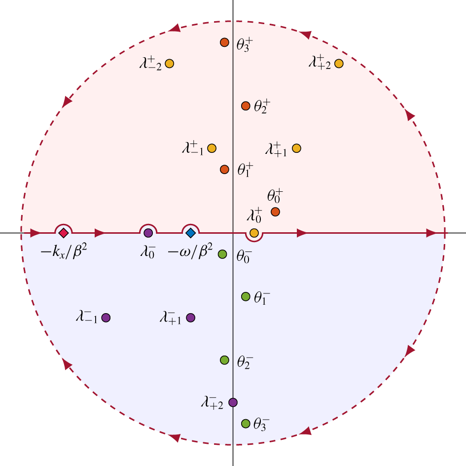
We first calculate
 $$\begin{eqnarray}\displaystyle \unicode[STIX]{x1D719}_{u,u}(x,y) & = & \displaystyle \int _{-\infty }^{\infty }D^{(1,3)}(\unicode[STIX]{x1D6FE})A_{u}(x,y;\unicode[STIX]{x1D6FE})\,\text{d}\unicode[STIX]{x1D6FE}\nonumber\\ \displaystyle & = & \displaystyle -2\unicode[STIX]{x03C0}\int _{-\infty }^{\infty }\{D^{(1,3)}(\unicode[STIX]{x1D6FE})K_{+}(\unicode[STIX]{x1D6FE})\}\,K_{-}(\unicode[STIX]{x1D6FE})\,\frac{\text{e}^{\text{i}(d-x)\unicode[STIX]{x1D6FE}+\text{i}\unicode[STIX]{x1D70E}}\cos (\unicode[STIX]{x1D701}y)}{K_{n}(\unicode[STIX]{x1D6FE})}\,\text{d}\unicode[STIX]{x1D6FE}.\end{eqnarray}$$
 Inspection of (3.11) shows that  $|D^{(1,3)}(\unicode[STIX]{x1D6FE})K_{+}(\unicode[STIX]{x1D6FE})|\rightarrow 0$ as $|\unicode[STIX]{x1D6FE}|\rightarrow \infty$ except at the poles at $\unicode[STIX]{x1D703}_{n}^{+}$ and $-k_{x}/\unicode[STIX]{x1D6FD}^{2}$. Consequently, we may close the above integral in ${\mathcal{L}}^{+}$ if $x<d$ and in ${\mathcal{L}}^{-}$ if $x>d$. Accordingly, we obtain for $x<d$
$x<d$
 $$\begin{eqnarray}\displaystyle \unicode[STIX]{x1D719}_{u,u}(x,y)=-2\unicode[STIX]{x03C0}\text{i}\mathop{\sum }_{n=0}^{\infty }{\mathcal{B}}_{n}A_{u}(x,y;\unicode[STIX]{x1D703}_{n}^{+})+2\unicode[STIX]{x03C0}\text{i}\mathop{\sum }_{m=-\infty }^{\infty }D^{(1,3)}(\unicode[STIX]{x1D706}_{m}^{+})A_{u}^{r}(x,y;\unicode[STIX]{x1D706}_{m}^{+}), & & \displaystyle \nonumber\end{eqnarray}$$
 and for  $x>d$,
 $$\begin{eqnarray}\displaystyle \unicode[STIX]{x1D719}_{u,u}(x,y)=-2\unicode[STIX]{x03C0}\mathop{\sum }_{n=0}^{\infty }\frac{{\mathcal{A}}_{n}+{\mathcal{C}}_{n}}{\unicode[STIX]{x1D703}_{n}^{-}+\unicode[STIX]{x1D714}/\unicode[STIX]{x1D6FD}^{2}}A_{u}(x,y;\unicode[STIX]{x1D703}_{n}^{-})-\frac{w_{0}A_{u}(x,y;-k_{x}/\unicode[STIX]{x1D6FD}^{2})}{2\unicode[STIX]{x03C0}K(-k_{x}/\unicode[STIX]{x1D6FD}^{2})}. & & \displaystyle \nonumber\end{eqnarray}$$
We proceed by considering
 $$\begin{eqnarray}\displaystyle \unicode[STIX]{x1D719}_{u,d}(x,y) & = & \displaystyle \int _{-\infty }^{\infty }D^{(1,3)}(\unicode[STIX]{x1D6FE})A_{d}(x,y;\unicode[STIX]{x1D6FE})\,\text{d}\unicode[STIX]{x1D6FE}\nonumber\\ \displaystyle & = & \displaystyle -2\unicode[STIX]{x03C0}\int _{-\infty }^{\infty }\{D^{(1,3)}(\unicode[STIX]{x1D6FE})K_{+}(\unicode[STIX]{x1D6FE})\}\,K_{-}(\unicode[STIX]{x1D6FE})\,\frac{-\text{e}^{-\text{i}\unicode[STIX]{x1D6FE}x}\cos (\unicode[STIX]{x1D701}(y-s))}{K_{n}(\unicode[STIX]{x1D6FE})}\,\text{d}\unicode[STIX]{x1D6FE}.\nonumber\end{eqnarray}$$
 Using a similar argument to the analysis for (C 1), we close the above integral in  ${\mathcal{L}}^{-}$ if $x>0$ in ${\mathcal{L}}^{+}$ if $x<0$. Consequently, for $x>0$ we obtain
 $$\begin{eqnarray}\displaystyle \unicode[STIX]{x1D719}_{u,d}(x,y)=-2\unicode[STIX]{x03C0}\mathop{\sum }_{n=0}^{\infty }\frac{{\mathcal{A}}_{n}+{\mathcal{C}}_{n}}{\unicode[STIX]{x1D703}_{n}^{-}+\unicode[STIX]{x1D714}/\unicode[STIX]{x1D6FD}^{2}}A_{d}(x,y;\unicode[STIX]{x1D703}_{n}^{-})-\frac{w_{0}A_{d}(x,y;-k_{x}/\unicode[STIX]{x1D6FD}^{2})}{2\unicode[STIX]{x03C0}K(-k_{x}/\unicode[STIX]{x1D6FD}^{2})}, & & \displaystyle \nonumber\end{eqnarray}$$
 and for  $x<0$ we obtain
 $$\begin{eqnarray}\displaystyle \unicode[STIX]{x1D719}_{u,d}(x,y)=-2\unicode[STIX]{x03C0}\text{i}\mathop{\sum }_{n=0}^{\infty }{\mathcal{B}}_{n}A_{d}(x,y;\unicode[STIX]{x1D703}_{n}^{+})+2\unicode[STIX]{x03C0}\text{i}\mathop{\sum }_{m=-\infty }^{\infty }D^{(1,3)}(\unicode[STIX]{x1D706}_{m}^{+})A_{d}^{r}(x,y;\unicode[STIX]{x1D706}_{m}^{+}). & & \displaystyle \nonumber\end{eqnarray}$$
We now consider
 $$\begin{eqnarray}\displaystyle \unicode[STIX]{x1D719}_{d,u}(x,y) & = & \displaystyle \int _{-\infty }^{\infty }D^{(2,4)}(\unicode[STIX]{x1D6FE})A_{u}(x,y;\unicode[STIX]{x1D6FE})\,\text{d}\unicode[STIX]{x1D6FE}\nonumber\\ \displaystyle & = & \displaystyle -2\unicode[STIX]{x03C0}\int _{-\infty }^{\infty }\{D^{(2,4)}(\unicode[STIX]{x1D6FE})\text{e}^{-2\text{i}\unicode[STIX]{x1D6FE}}K_{-}(\unicode[STIX]{x1D6FE})\}K_{+}(\unicode[STIX]{x1D6FE})\frac{\text{e}^{\text{i}(d+2-x)\unicode[STIX]{x1D6FE}+\text{i}\unicode[STIX]{x1D70E}^{\prime }}\cos (\unicode[STIX]{x1D701}y)}{K_{n}(\unicode[STIX]{x1D6FE})}\,\text{d}\unicode[STIX]{x1D6FE}.\nonumber\end{eqnarray}$$
 Following a similar argument to (C 1),  $|D^{(2,4)}(\unicode[STIX]{x1D6FE})\text{e}^{-2\text{i}\unicode[STIX]{x1D6FE}}K_{-}(\unicode[STIX]{x1D6FE})|\rightarrow 0$ as $|\unicode[STIX]{x1D6FE}|\rightarrow \infty$ except at the poles at $-\unicode[STIX]{x1D714}/\unicode[STIX]{x1D6FD}^{2}$, $-k_{x}/\unicode[STIX]{x1D6FD}^{2}$ and $\unicode[STIX]{x1D703}_{n}^{\pm }$. Consequently, we close the integral in ${\mathcal{L}}^{+}$ if $x<d+2$ and in ${\mathcal{L}}^{-}$ if $x>d+2$. For $x<d+2$ we obtain
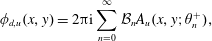 $$\begin{eqnarray}\displaystyle \unicode[STIX]{x1D719}_{d,u}(x,y)=2\unicode[STIX]{x03C0}\text{i}\mathop{\sum }_{n=0}^{\infty }{\mathcal{B}}_{n}A_{u}(x,y;\unicode[STIX]{x1D703}_{n}^{+}), & & \displaystyle \nonumber\end{eqnarray}$$
 and for  $x>d+2$ we obtain
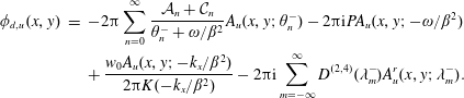 $$\begin{eqnarray}\displaystyle \unicode[STIX]{x1D719}_{d,u}(x,y) & = & \displaystyle -2\unicode[STIX]{x03C0}\mathop{\sum }_{n=0}^{\infty }\frac{{\mathcal{A}}_{n}+{\mathcal{C}}_{n}}{\unicode[STIX]{x1D703}_{n}^{-}+\unicode[STIX]{x1D714}/\unicode[STIX]{x1D6FD}^{2}}A_{u}(x,y;\unicode[STIX]{x1D703}_{n}^{-})-2\unicode[STIX]{x03C0}\text{i}PA_{u}(x,y;-\unicode[STIX]{x1D714}/\unicode[STIX]{x1D6FD}^{2})\nonumber\\ \displaystyle & & \displaystyle +\,\frac{w_{0}A_{u}(x,y;-k_{x}/\unicode[STIX]{x1D6FD}^{2})}{2\unicode[STIX]{x03C0}K(-k_{x}/\unicode[STIX]{x1D6FD}^{2})}-2\unicode[STIX]{x03C0}\text{i}\mathop{\sum }_{m=-\infty }^{\infty }D^{(2,4)}(\unicode[STIX]{x1D706}_{m}^{-})A_{u}^{r}(x,y;\unicode[STIX]{x1D706}_{m}^{-}).\nonumber\end{eqnarray}$$
The final integral is
 $$\begin{eqnarray}\displaystyle \unicode[STIX]{x1D719}_{d,d}(x,y) & = & \displaystyle \int _{-\infty }^{\infty }D^{(2,4)}(\unicode[STIX]{x1D6FE})\text{e}^{-\text{i}\unicode[STIX]{x1D6FE}x}A_{d}(x,y;\unicode[STIX]{x1D6FE})\,\text{d}\unicode[STIX]{x1D6FE}\nonumber\\ \displaystyle & = & \displaystyle -2\unicode[STIX]{x03C0}\int _{-\infty }^{\infty }\{D^{(2,4)}(\unicode[STIX]{x1D6FE})\text{e}^{-2\text{i}\unicode[STIX]{x1D6FE}}K_{-}(\unicode[STIX]{x1D6FE})\}K_{+}(\unicode[STIX]{x1D6FE})\frac{-\text{e}^{\text{i}(2-x)\unicode[STIX]{x1D6FE}}\cos (\unicode[STIX]{x1D701}(y-s))}{K_{n}(\unicode[STIX]{x1D6FE})}\,\text{d}\unicode[STIX]{x1D6FE}.\nonumber\end{eqnarray}$$
 Using similar arguments to the previous integrals, we close the above integral in  ${\mathcal{L}}^{+}$ if $x<2$ and in ${\mathcal{L}}^{-}$ if $x>2$. Consequently, for $x<2$ we obtain
 $$\begin{eqnarray}\displaystyle \unicode[STIX]{x1D719}_{d,d}(x,y)=2\unicode[STIX]{x03C0}\text{i}\mathop{\sum }_{n=0}^{\infty }{\mathcal{B}}_{n}A_{d}(x,y;\unicode[STIX]{x1D703}_{n}^{+}), & & \displaystyle \nonumber\end{eqnarray}$$
 and for  $x>2$ we obtain
 $$\begin{eqnarray}\displaystyle \unicode[STIX]{x1D719}_{d,d}(x,y) & = & \displaystyle 2\unicode[STIX]{x03C0}\mathop{\sum }_{n=0}^{\infty }\frac{{\mathcal{A}}_{n}+{\mathcal{C}}_{n}}{\unicode[STIX]{x1D703}_{n}^{-}+\unicode[STIX]{x1D714}/\unicode[STIX]{x1D6FD}^{2}}A_{d}(x,y;\unicode[STIX]{x1D703}_{n}^{-})+2\unicode[STIX]{x03C0}\text{i}PA_{d}(x,y;-\unicode[STIX]{x1D714}/\unicode[STIX]{x1D6FD}^{2})\nonumber\\ \displaystyle & & \displaystyle +\,\frac{w_{0}A_{d}(x,y;-k_{x}/\unicode[STIX]{x1D6FD}^{2})}{2\unicode[STIX]{x03C0}K(-k_{x}/\unicode[STIX]{x1D6FD}^{2})}-2\unicode[STIX]{x03C0}\text{i}\mathop{\sum }_{m=-\infty }^{\infty }D^{(2,4)}(\unicode[STIX]{x1D706}_{m}^{-})A_{d}^{r}(x,y;\unicode[STIX]{x1D706}_{m}^{-}).\nonumber\end{eqnarray}$$
Summing the contributions from each integral yields the full Fourier inversion in § 3.1.


 Open access