


1. Introduction
Pathogenic bacteria are a persistent threat to human health incurring a heavy cost on the healthcare system (Jean et al. Reference Jean, Tanya, Lin and MacDonald1996). The motility of bacteria is an essential mechanism with which pathogens reach the membranes of susceptible cells or form harmful biofilms on tissues and implants (Ottemann & Miller Reference Ottemann and Miller1997; Jarrell & McBride Reference Jarrell and McBride2008; Kearns Reference Kearns2010). The majority of the cells and tissues prone to pathogenic infections in the human body are lined with a multi-scale complex biological fluid. For instance, the mucosal surfaces in the body including the epithelial cells in the respiratory tract, the human intestines, the urinary tract, the eyes etc. are lined with a slimy hydro-gel known as mucus (McShane et al. Reference McShane, Bath, Jaramilo, Ridley, Walsh, Evans, Thornton and Ribbeck2021). These are complex fluids, meaning that they possess a microstructure (a porous, mesh-like polymer network resulting from entanglement) and often exhibit non-Newtonian rheology, which is a function of length scale. Therefore, a fundamental understanding of how the rheology and microstructure of biological fluids affect the motion of a swimming bacterium has applications ranging from designing therapeutic techniques by changing the properties of the biological fluids (Werlang, Carcarmo-Oyarce & Ribbeck Reference Werlang, Carcarmo-Oyarce and Ribbeck2019) to designing synthetic swimmers for targeted drug delivery (Huang et al. Reference Huang, Uslu, Katsamba, Lauga, Sakar and Nelson2019; Xiea et al. Reference Xiea, Xiab, Lia, Moa, Chena and Lia2020; Ghosh & Ghosh Reference Ghosh and Ghosh2021), and developing gene regulatory programs for bacteria to name a few.
In this work, we develop a two-fluid model, where the complex fluid is modelled as a coupled, interpenetrating medium of two Newtonian fluids, and we analyse the motion of a flagellated bacterium (like Escherichia coli) in it. This Newtonian model captures the effect of the microstructure present in these complex biological fluids by allowing for a relative motion between the solvent and polymer. This differential motion is relevant because the length scale of the the entangled polymer network in such fluids is comparable to the diameter of the flagellar bundle of the bacterium. This results in the bundle forcing the solvent and the polymer differently, leading to differential response of the two fluids. The model can be easily extended to a complex fluid with non-Newtonian rheology, using which, the combined effects of microstructure and non-Newtonian rheology of the complex biological fluid on the swimming bacterium can be analysed by numerical simulations.
The motion of swimming microorganisms in Newtonian fluids has been a well-studied problem for decades (Berg & Anderson Reference Berg and Anderson1973; Purcell Reference Purcell1977; Lauga & Powers Reference Lauga and Powers2009; Subramanian & Nott Reference Subramanian and Nott2011). Microorganisms, owing to their small size, essentially swim in a low-Reynolds-number ( $Re$) environment, where viscous effects dominate inertial effects. In this Stokesian regime, the fluid flow is quasi-steady and linear making the flow (kinematically) reversible. Therefore, the usual macroscopic swimming strategies, like periodic paddling motion, are ineffective and will result in no net motion (Ludwig Reference Ludwig1930). To overcome this, microorganisms have evolved several successful propulsion strategies. There are many variations of these strategies among swimming microorganisms and several types of organisms exist that swim in low-Reynolds-number environments using different means (Lauga & Powers Reference Lauga and Powers2009; Subramanian & Nott Reference Subramanian and Nott2011). In this work, we restrict our attention to the motion of flagellated bacteria, like Escherichia coli (E. coli).
Berg & Anderson (Reference Berg and Anderson1973) showed that bacteria like E. coli break the Stokesian symmetry by means of a rotating appendage – the flagellar bundle, made up of multiple individual flagellar filaments. The flagellum is a slender filament attached to the head of the bacterium by a hook and rotated by a molecular motor (Berg Reference Berg2003). E. coli have prolate spheroidal heads of typical length 2–3  $\mathrm {\mu }$m and width 1–2 $\mathrm {\mu }$m. The flagellar filament of E. coli has a diameter of $\approx$20 nm and traces out a helix with contour length $\approx$10 $\mathrm {\mu }$m. In the absence of external forces and moments, the helix is typically left-handed with a pitch $\approx$2.5 $\mathrm {\mu }$m and a helical diameter $\approx$0.5 $\mathrm {\mu }$m (Turner, Ryu & Berg Reference Turner, Ryu and Berg2000). There are typically $\sim$5–8 flagellar filaments per cell of E. coli. When all the motors rotate in the same direction, all the filaments wrap into a helical bundle of diameter $\approx$60–80 nm and rotate in unison. This generates thrust due to an anisotropy in the drag experienced by the flagellar bundle (Lauga & Powers Reference Lauga and Powers2009), propelling the bacterium forward – the motion being called a run. When one or more of the motors reverse, the corresponding filaments leave the bundle and undergo ‘polymorphic’ transformations which change the swimming direction of the cell – this process being called tumbling. Thus, bacteria exhibit run and tumble motions in a fluid medium. This motion of bacteria in Newtonian fluids has been successfully modelled by resistive force theory (RFT) (Gray & Hancock Reference Gray and Hancock1955; Chwang & Wu Reference Chwang and Wu1971) and slender body theory (SBT) (Batchelor Reference Batchelor1970; Cox Reference Cox1970; Johnson Reference Johnson1980), which treat the helical flagellar bundle as a slender fibre moving through a viscous fluid. Recently, these theories for slender objects have been experimentally verified by Rodenborn et al. (Reference Rodenborn, Chen, Swinney, Liu and Zhang2013), by comparing experimentally measured values of thrust, drag and torque on a slender helical fibre that was rotated and translated in a viscous fluid with those values predicted by the theories.
While the preceding discussion addressed bacterial motion in Newtonian fluids, bacterial motility in complex fluids is still an open question in many ways. There are several interesting characteristics exhibited by swimming bacteria in complex fluids (Spagnolie & Underhill Reference Spagnolie and Underhill2023). While the class of complex fluids is enormous, most of the attention so far has been centred on one type of complex fluid, namely, polymer solutions. The major motivation for this is that several biological fluids, which these organisms typically encounter, are polymer solutions (Lauga & Powers Reference Lauga and Powers2009). In these fluids, for instance, bacteria are known to swim in straighter trajectories (Patteson et al. Reference Patteson, Gopinath, Goulian and Araatia2015), exhibit less frequent tumbling (Qu & Breuer Reference Qu and Breuer2020) and form a flagellar bundle more rapidly (Qu et al. Reference Qu, Temel, Henderikx and Breuer2018).
A fundamental understanding of the aforementioned phenomena necessitates a thorough understanding of the swimming motion of bacteria in polymer solutions. Polymer solutions are non-Newtonian fluids possessing three primary characteristics, namely: (i) viscoelasticity; (ii) shear-dependent viscosity; and (iii) a microstructure, and several studies have tried to understand the relative importance of these factors on the swimming motion of bacteria. Earlier theoretical studies on simple geometries, like waving sheets (Lauga Reference Lauga2007) and waving filaments (Fu, Powers & Wolgemuth Reference Fu, Powers and Wolgemuth2007a; Fu, Wolgemuth & Powers Reference Fu, Wolgemuth and Powers2009) in viscoelastic polymer solutions with shear-independent viscosities (Boger fluids) as the swimming media, showed that the propulsive velocities of the sheets and fibres are smaller in viscoelastic fluids than in Newtonian solvents since the polymer solutions always have a larger viscosity than the Newtonian solvents (even with shear thinning). However, later theoretical studies (Teran, Fauci & Shelley Reference Teran, Fauci and Shelley2010; Spagnolie, Liu & Powers Reference Spagnolie, Liu and Powers2013; Riley & Lauga Reference Riley and Lauga2014; Thomases & Guy Reference Thomases and Guy2014) on undulating sheets and helices, and experimental studies (Liu, Powers & Breuer Reference Liu, Powers and Breuer2011; Espinosa-Garcia, Lauga & Zenir Reference Espinosa-Garcia, Lauga and Zenir2013) on artificial swimmers, extended the results of the earlier ones to show that swimming enhancement can result in a viscoelastic (Boger) media due to several factors like large amplitude oscillations (Liu et al. Reference Liu, Powers and Breuer2011; Spagnolie et al. Reference Spagnolie, Liu and Powers2013), stress-singularities at filament/sheet ends (Teran et al. Reference Teran, Fauci and Shelley2010), dynamic balance of stresses (Riley & Lauga Reference Riley and Lauga2014), flexibility (Espinosa-Garcia et al. Reference Espinosa-Garcia, Lauga and Zenir2013) and (elastic) stress-asymmetry (Thomases & Guy Reference Thomases and Guy2014). These results suggested that in viscoelastic media, the motion of microswimmers is highly dependent on the geometry of the swimmer, the generated waveform and the relaxation time of the medium, owing to its nonlinearity.
Experiments with actual bacteria, such as E. coli, in shear-thinning, viscoelastic polymer solutions reported specifically that they swim at higher speeds than in Newtonian liquids having the same shear viscosity (Berg & Turner Reference Berg and Turner1979; Patteson et al. Reference Patteson, Gopinath, Goulian and Araatia2015; Qu et al. Reference Qu, Temel, Henderikx and Breuer2018). These studies proposed that shear-thinning of the polymer near the flagellar bundle, owing to its fast rotation, contributes most to the observed swimming enhancement of bacteria for polymers with small relaxation times (low  $De$;
$De$;  $De$ being the Deborah number defined as the ratio of the polymer relaxation time to the flow time scale), while viscoelastic effects like normal stress differences and elastic stresses contribute significantly to enhancement with high relaxation time polymers (high $De$) (Qu & Breuer Reference Qu and Breuer2020). This has motivated theoretical models (Man & Lauga Reference Man and Lauga2015) that use a two-layer approximation of the polymer solutions at low $De$ – with a layer of lower viscosity near the flagellar bundle and a layer of larger viscosity on the scale of the cell – and explain the observed experimental results. The experiments and the theoretical model mentioned above correspond to viscoelastic polymer solutions, with small polymer concentrations ( $c < c^*$; $c$ is polymer concentration and $c^*$ is overlap concentration) as the swimming media, but biological fluids are usually concentrated polymer solutions ( $c \geq c^*$).
There are not many experimental or theoretical studies that address the fluid mechanics of bacterial motion in concentrated polymer solutions. Berg & Turner (Reference Berg and Turner1979) first showed that bacteria can swim with higher velocities in concentrated polymer solutions, compared with polymer solutions of short chained polymers having the same viscosity, but they wrongly attributed this enhancement to the presence of bacteria-sized pores in the polymer network, which do not exist. Magariyama & Kudo (Reference Magariyama and Kudo2002) used this idea to develop a theory, which used different viscosities (resistances) for translation and rotation of both the head and flagellar bundle in a fluid medium modelling the entangled polymer solution, and predicted qualitatively similar trends for swimming velocity, but their model also resulted in a non-physical trend, wherein the angular velocity of the bacterial head was found to increase with viscosity.
More recently, an experimental study by Martinez et al. (Reference Martinez, Schwarz-Link, Reufer, Wilson, Morozov and Poon2014) also showed that an enhancement in swimming speed is observed in a concentrated polymer solution ( $c \sim c^*$), and the explanation offered was a combination of shear thinning and depletion of polymers from the vicinity of the flagellar bundle, essentially making the flagellar bundle swim through a fluid of small viscosity. However, this explanation is not consistent with the fact that for the polymer solution used in the experiment (Martinez et al. Reference Martinez, Schwarz-Link, Reufer, Wilson, Morozov and Poon2014), rheological measurements do not show significant shear thinning at the shear rates assumed near the flagellar bundle. Moreover, the authors do not provide any explanation for depletion of polymers near the flagellar bundle. A computational work by Zottl & Yeomans (Reference Zottl and Yeomans2019) on a bacterium swimming through a concentrated polymer solution showed an enhancement due to depletion of polymers near the flagellar bundle. The authors used coarse-grained molecular dynamics (MD) simulations, where the polymer was modelled as a chain of spherical (monomer) beads which were large, resulting in a few degrees of freedom for the chain, and the observed depletion near the bundle may therefore be an overestimate that does not correspond to the actual scenario.
Recently, the work of Kamdar et al. (Reference Kamdar, Shin, Leishangthem, Francis, Xu and Cheng2022) has shown that, in the dilute and semi-dilute regimes,  $c \lesssim c^*$, the colloidal nature of the polymer solutions quantitatively explain the observed swimming enhancement in the aforementioned experiments, where the enhancement scales with the radius of gyration of the polymer chains, and polymer dynamics may not be essential for capturing the phenomena. This suggests that the length scale of the polymer chains (microstructure) may be more relevant in this regime. Notably, the results of Kamdar et al. (Reference Kamdar, Shin, Leishangthem, Francis, Xu and Cheng2022) with colloidal suspensions also quantitatively explain other features, namely, straighter trajectories of bacteria, reduced tumbling frequency etc., which were observed in the earlier experiments with dilute polymer solutions. Their findings seem to imply that the length scale of the polymer chains (microstructure) could be the most relevant parameter affecting the swimming velocity directly in dilute and semi-dilute polymer solutions, while viscoelasticity leads to other consequences like straight trajectories, reduced tumbling etc., which affect velocity indirectly.
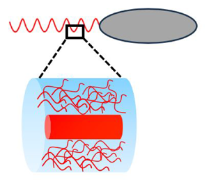
In concentrated polymer solutions, the question of relative importance of these characteristics on swimming motion is yet to be answered satisfactorily. Concentrated polymer solutions also exhibit shear-dependent viscosity and viscoelastic stresses, and crucially, they are entangled and possess a porous microstructure, where in some cases, the pore sizes may be comparable to the thickness of the flagellar bundle, but not the head of the bacterium. For instance, it is known that mucus has a microstructure that resembles a mesh, where the mucin filaments form a complicated network of entangled polymer fibres with pores ( $\sim$100 nm (in humans)–400 nm (in horses), see Kirch et al. Reference Kirch, Schneider, Abou, Hopf, Schaefer, Schneider, Schall, Wagner and Lehr2012), which are larger than the flagellar bundle diameter ( $\sim$60–80 nm, see Turner et al. Reference Turner, Ryu and Berg2000) and are filled with the Newtonian solvent (Cone Reference Cone2009; Lai et al. Reference Lai, Wang, Hida, Cone and Hanes2011). Notably, unlike dilute solutions, their viscoelastic response and shear-dependent viscosity cannot be explained by analogy to colloidal suspensions, and therefore the model of Kamdar et al. (Reference Kamdar, Shin, Leishangthem, Francis, Xu and Cheng2022) cannot be applied. Also, the theoretical models mentioned earlier (Magariyama & Kudo Reference Magariyama and Kudo2002; Martinez et al. Reference Martinez, Schwarz-Link, Reufer, Wilson, Morozov and Poon2014; Man & Lauga Reference Man and Lauga2015; Zottl & Yeomans Reference Zottl and Yeomans2019) assume bacteria-sized pores, significant shear thinning or depletion near the flagellar bundle, and these assumptions are inappropriate for an entangled polymer solution like mucus. In such a medium, rather than a physical depletion of polymers or shear thinning, one has the flagellar bundle interacting differently with the solvent and polymer, exerting different forces on them, owing to the porous polymer network with pores having nearly the same size as the bundle diameter. This differential response results in a relative motion between the solvent and polymer near the bundle. Some earlier studies of waving sheets in entangled networks (Fu, Shenoy & Powers Reference Fu, Shenoy and Powers2010; Wada Reference Wada2010; Du et al. Reference Du, Keener, Guy and Fogelson2012) have used this idea, with the polymer being treated as a purely elastic medium. A similar idea was used in the computational study by Wrobel et al. (Reference Wrobel, Lynch, Barrett, Fauci and Cortez2016), where the polymer was modelled as an elastic network constructed out of a collection of cross-linked regularised Stokeslets, with the links between them being linearly viscoelastic. The theoretical studies have not considered helical geometries, like the flagellar bundle of a bacterium, which requires a slender body treatment, and the polymer network in biological fluids like mucus are not perfectly elastic, as these studies assume.
In this work, we propose a two-fluid model to accurately capture this differential response of solvent and polymer, caused by the microstructure in an entangled polymer solution like mucus. In our model, the polymer and solvent are both treated as Newtonian fluids with different viscosities  $\mu _p$ and $\mu _s$; $\lambda = \mu _p/\mu _s$ being the viscosity ratio. This Newtonian approximation for the polymer is valid if the polymer has small non-Newtonian effects, with $De \ll 1$, an assumption that is fairly representative of the polymer solutions used in the experiments of Martinez et al. (Reference Martinez, Schwarz-Link, Reufer, Wilson, Morozov and Poon2014) and Qu & Breuer (Reference Qu and Breuer2020). In such a scenario, the flagellar bundle directly forces the solvent present in the pores, which then transmits the stresses to the polymer. These two fluids therefore move relative to each other leading to a Darcy drag term in the governing equations and hence a screening length $L_B$, within which the relative velocity of the two fluids decays. The resulting equations for the relative velocity of the solvent and polymer are similar to the Brinkman equations for flow through porous media (Brinkman Reference Brinkman1947). Some earlier studies have studied the motion of a slender body (Howells Reference Howells1998; Leshansky Reference Leshansky2009) and a bacterium (Chen et al. Reference Chen, Lordi, Taylor and Pak2021) in a Brinkman medium using RFT. There have also been a slender body treatment of helical fibres (Ho, Leiderman & Olsen Reference Ho, Leiderman and Olsen2019) and a study of squirmers in Brinkman medium (Nganguia & Pak Reference Nganguia and Pak2018). In these studies, the pores result from a sparse random distribution of rigid bodies, whereas in this study, the porous structure results from polymers, which are also subject to motion.
We first analyse the motion of a slender helical fibre in such a medium using SBT and then use RFT to analyse the motion of a bacterium with a helical flagellar bundle in this medium. Our analysis indicates that bacterial motion is sensitive to the nature of the interaction between the flagellar bundle and the polymer, and predicts an increased drag anisotropy. This, in turn, leads to an enhancement in the swimming speed, compared with the case where the polymer solution is treated as a continuum mixture – a Newtonian medium with viscosity  $\mu _s(1 + \lambda )$. We model two physical scenarios, corresponding to two possible polymer–flagellar bundle interactions: (i) a case where the polymer slips past the bundle and (ii) a case where the polymer is not subject to any direct continuum forcing by the bundle (no interaction).
2. Two-fluid model of the polymer solution
In this section, we describe the two-fluid model of a polymer solution and analyse the motion of a sphere through it to explain its features. Two-fluid models for polymer solutions were first introduced by Doi (Reference Doi1990). While typical mixture models of polymer solutions assume that the polymers and solvent move with a common velocity, Doi's two-fluid model allows for relative motion between the polymer and the solvent, owing to the fact that under certain conditions, inhomogeneous fluid flow can create polymer concentration gradients and lead to diffusion of polymers relative to the solvent flow. The model describes a polymer solution composed of a Newtonian solvent phase with viscosity  $\mu _s$ and a polymer phase with the two phases coexisting as interpenetrating continua. In general, the model permits a non-uniform concentration for the polymer, while treating the polymer as a non-Newtonian medium. Such models have been successfully used in other phenomena involving entangled polymer solutions, where such a differential response in solvent and polymer may arise (e.g. electroconvection of electrolytes with polymer additives Tikekar et al. Reference Tikekar, Li, Archer and Koch2018, shear banding phenomenon in concentrated polymer solutions Cromer et al. Reference Cromer, Villet, Frederickson and Leal2013 and swelling of polymeric gels Wang, Li & Hu Reference Wang, Li and Hu1997). In all these cases, a non-equilibrium forcing results in the polymer having a different velocity than the solvent. The predictions of these models have also been shown to match with experimental observations (Doi Reference Doi2009; Burroughs et al. Reference Burroughs, Zhang, Shetty, Bates, Leal and Helgeson2021).
In this work, the polymer is modelled as a Newtonian fluid with uniform concentration (as this fairly represents the conditions found in earlier experiments by Martinez et al. Reference Martinez, Schwarz-Link, Reufer, Wilson, Morozov and Poon2014; Qu & Breuer Reference Qu and Breuer2020), having a different viscosity  $\mu _p$, where the viscosity is equivalent to the polymer's contribution to the zero-shear viscosity of the polymer solution. The polymer and the solvent are allowed to move relative to each other and the inertial effects in both fluids are considered to be negligible, with the Reynolds number ( $Re$) based on both $\mu _s$ and $\mu _p$ being small; $Re \ll 1$. Here, the non-equilibrium condition between the polymer and solvent is created by the different forces they experience at the boundary of the rotating flagellar bundle, because of the microstructure ‘seen’ by the flagellar bundle. Unlike Doi (Reference Doi1990), we consider the polymer to have a constant concentration and an incompressible mass conservation equation. This condition can be approximated in the model of Doi (Reference Doi1990) if the osmotic susceptibility of the polymer is small, so that the osmotic pressure (termed $p_p$ here) takes on whatever values are needed to impose the incompressibility of the polymer phase. The governing equations of our two-fluid model are given by
 $$\begin{gather} \boldsymbol{\nabla}\boldsymbol{\cdot}\boldsymbol{u}_s = 0,\quad \boldsymbol{\nabla}\boldsymbol{\cdot}\boldsymbol{u}_p = 0 = 0, \end{gather}$$
 $$\begin{gather}\mu_s \nabla^2 \boldsymbol{u}_s - \nabla p_s - \xi (\boldsymbol{u}_s - \boldsymbol{u}_p) = 0, \end{gather}$$
 $$\begin{gather}\mu_p \nabla^2 \boldsymbol{u}_p - \nabla p_p + \xi (\boldsymbol{u}_s - \boldsymbol{u}_p) = 0, \end{gather}$$
where  $\boldsymbol {u}_s$, $\boldsymbol {u}_p$, $p_s$ and $p_p$ correspond to the solvent and polymer phase velocities and pressures, respectively, and $\xi$ is the Darcy resistance coefficient defined as $\xi = \mu _s/L_B^2$, where $L_B$ is the screening length of the two-fluid medium. As noted earlier, the form of the equations is similar to Brinkman's equations in a porous medium (Brinkman Reference Brinkman1947), except that here, the polymers forming the porous network are capable of flowing. Thus, $L_B$ can be considered to be the length scale of hydrodynamic coupling in the polymer solution, which is $O(\phi ^{-1/2} \log \phi ^{1/2})$, $\phi$ being the polymer volume fraction, if the polymers are assumed to be fibres of finite length randomly oriented in space (Howells Reference Howells1998). The above equations can be written in dimensionless form as
 $$\begin{gather} \boldsymbol{\nabla}\boldsymbol{\cdot}\boldsymbol{u}_s = 0,\quad \boldsymbol{\nabla}\boldsymbol{\cdot}\boldsymbol{u}_p = 0, \end{gather}$$
 $$\begin{gather}\nabla^2 \boldsymbol{u}_s - \nabla p_s - \frac{1}{L_B^2}(\boldsymbol{u}_s - \boldsymbol{u}_p) = 0 , \end{gather}$$
 $$\begin{gather}\lambda \nabla^2 \boldsymbol{u}_p - \lambda \nabla p_p + \frac{1}{L_B^2}(\boldsymbol{u}_s - \boldsymbol{u}_p) = 0, \end{gather}$$
where we have non-dimensionalised the lengths with a characteristic length scale  $l$, the velocity with characteristic velocity scale $U$, and the solvent and polymer pressures with $\mu _s U / l$ and $\mu _p U/l$. Note that $L_B$ in (2.5), (2.6) is dimensionless (equal to $L_B/l$) and should be considered as such in the sections that follow, unless otherwise stated.
2.1. A translating and rotating sphere in the two-fluid medium
Before embarking on the more challenging problems of studying the motion of a helix and then a bacterium in the two-fluid medium, we first study a sphere of radius ‘ $a$’ moving with a velocity $\boldsymbol {U}$ and rotating with an angular velocity $\boldsymbol {\omega }$ through the quiescent two-fluid medium to gain insights into the response of the medium. A similar problem has been solved by Fu, Shenoy & Powers (Reference Fu, Shenoy and Powers2007b) for a sphere translating in a a purely elastic polymer, and by Moradi, Shi & Nazockdast (Reference Moradi, Shi and Nazockdast2022) for a sphere moving in a linearly viscoelastic polymer. Our model considers a Newtonian polymer phase. As mentioned in the introduction, our calculations consider two sets of boundary conditions corresponding to two physical scenarios: (i) the polymer slipping past the solid body and (ii) the polymer not interacting with the solid body. The first case is relevant when the body moves through an entangled polymer solution with pore sizes comparable to the characteristic length scale of the body (in this example, this is the sphere diameter $2a$) and the second case is relevant when the pore size is much larger than the characteristic length scale of the body, so that the polymer is not directly forced by the moving body, but is forced indirectly by the solvent which is affected by the motion. The solvent satisfies no-slip in both cases. Thus, the boundary conditions for the first case are
 $$\begin{gather} \boldsymbol{u}_s, \boldsymbol{u}_p \rightarrow 0 \quad \text{as} \ r \rightarrow \infty, \end{gather}$$
 $$\begin{gather}\boldsymbol{u}_s = \boldsymbol{U} + \boldsymbol{\omega} \times \boldsymbol{r} \quad \text{at} \ r = a, \end{gather}$$
 $$\begin{gather}\boldsymbol{u}_p\boldsymbol{\cdot}\boldsymbol{n} = \boldsymbol{U}\boldsymbol{\cdot}\boldsymbol{n} \quad \text{at} \ r = a, \end{gather}$$
 $$\begin{gather}(\boldsymbol{I} - \boldsymbol{nn})\boldsymbol{\cdot}(\boldsymbol{\sigma}_p\boldsymbol{\cdot}\boldsymbol{n}) = 0 \quad \text{at} \ r = a, \end{gather}$$
which are respectively the far-field conditions, no slip condition for the solvent, no penetration condition for the polymer and zero tangential polymer stress on the sphere surface (a completely slipping polymer). Here,  $r = |\boldsymbol {r}|$ is the radial distance and $\boldsymbol {n} = \boldsymbol {r}/r$ is the unit normal. Therefore, the polymer will not resist tangential motion (shearing) but will resist normal motion (pressure).
The solution procedure and the exact expressions for the velocities and pressures for both fluids are given in supplementary Appendix A available at https://doi.org/10.1017/jfm.2024.1069, and the procedure involves solving the above set of coupled partial differential equations by defining two new fields  $\boldsymbol {u}_m = \boldsymbol {u}_s + \lambda \boldsymbol {u}_p$ and $\boldsymbol {u}_d = \boldsymbol {u}_p - \boldsymbol {u}_s$ (similarly for $p_m$, $p_d$ and other variables). These two fields define a mixture field satisfying Stokes equations and a difference field satisfying Brinkman equations, for which solutions are easily derived. Figure 1 shows the normalised drag force on a translating sphere and the torque on a rotating sphere as functions of the screening length $L_B/a$ for different values of $\lambda$, where the normalisation is with respect to drag and torque in the solvent (of viscosity $\mu _s$). From the figure, we see that as the screening length approaches zero, the dimensional drag on the sphere approaches $6 {\rm \pi} \mu _s |\boldsymbol {U}| (1 + \lambda ) a$ for translation and the torque approaches $8 {\rm \pi} \mu _s a^3 (1+\lambda ) |\boldsymbol {\omega }|$ for the case of rotation. These are the corresponding values for drag and torque, in a medium that is a mixture of the two fluids (same as a single-fluid medium with viscosity $\mu _s(1 + \lambda )$; hereby just referred to as the mixture). This suggests that for $L_B/a \rightarrow 0$, the medium behaves like a mixture implying that there is no relative motion between the two fluids, even if one of them is allowed to slip past the solid boundary, i.e. taking this limit is the same as using a no-slip boundary condition for both fluids. The other limit of $L_B/a \rightarrow \infty$ corresponds to the decoupled solvent and polymer acting independently of each other, which results in a dimensional drag and torque of $6 {\rm \pi} \mu _s |\boldsymbol {U}| (1 + {2 \lambda }/{3}) a$ and $8 {\rm \pi} \mu _s a^3 (1+{2\lambda }/{3}) |\boldsymbol {\omega }|$, respectively. The factor $2/3$ arises because, in this limit, the sphere acts like a bubble moving through the polymer on account of the zero tangential stress condition on the polymer. This calculation shows that one can go from a mixture-like behaviour to a completely decoupled behaviour of the two fluids using the two-fluid model.
Plots of (a) drag force normalised by  $F_N = 6 {\rm \pi} U \mu _s a$ on a sphere of radius $a$ translating with velocity $U$ and (b) torque normalised by $T_N = 8 {\rm \pi} \mu _s a^3 \omega$ on a sphere rotating with angular velocity $\omega$ in a two-fluid medium with a slipping polymer, as a function of $L_B/a$.

A similar calculation can be done for the second case, where there is no polymer–sphere interaction with the boundary conditions now given by
 $$\begin{gather} \boldsymbol{u}_s, \boldsymbol{u}_p \rightarrow 0 \quad \text{as} \ r \rightarrow \infty, \end{gather}$$
 $$\begin{gather}\boldsymbol{u}_s = \boldsymbol{U} + \boldsymbol{\omega} \times \boldsymbol{r}\quad \text{at} \ r = a, \end{gather}$$
 $$\begin{gather}\boldsymbol{\sigma}_p\boldsymbol{\cdot}\boldsymbol{n} = 0 \quad \text{at} \ r = a. \end{gather}$$
For this case, the plots of normalised drag and torque are given in figure 2, which are similar to those in figure 1 (the torque on the sphere being exactly the same). The primary difference between this scenario and the previous one arises in the drag force acting on the sphere in the limit of  $L_B/a \rightarrow \infty$, for which the drag on the sphere is $6 {\rm \pi} \mu _s |\boldsymbol {U}| a$. This is consistent with the fact that the polymer is not forced by the sphere and in the limit of large screening length, where the fluids act independently, only the solvent contributes to the drag.
Plots of (a) drag force normalised by  $F_N = 6 {\rm \pi} U \mu _s a$ on a sphere of radius $a$ translating with velocity $U$ and (b) torque normalised by $T_N = 8 {\rm \pi} \mu _s a^3 \omega$ on a sphere rotating with angular velocity $\omega$ in a two-fluid medium with no polymer–sphere interaction, as a function of $L_B/a$.

The takeaway from this sample calculation is that, using the two-fluid model, one can go from mixture-like behaviour (a single fluid with viscosity  $\mu _s + \mu _p$ – similar to the canonical treatment of polymer solutions) to completely decoupled behaviour of the two fluids by varying $L_B$. Thus, the screening length $L_B$ is equivalent to the characteristic length scale of the microstructure in the polymer solution. In the next section, we derive solutions for a slender helical fibre moving through the two-fluid medium, satisfying the same two sets of boundary conditions as the sphere, and analyse the effect of microstructure on its motion.
2.2. Fundamental solutions of the two-fluid equations
To derive the SBT in the two-fluid medium, we need the fundamental solutions for the two-fluid equations, which are derived here. The dimensionless governing equations are now given by
 $$\begin{gather} \nabla^2 \boldsymbol{u}_s - \nabla p_s - \frac{1}{L^2_B} (\boldsymbol{u}_s - \boldsymbol{u}_p) = \boldsymbol{F}_s \delta(\boldsymbol{r}), \end{gather}$$
 $$\begin{gather}\lambda \nabla^2 \boldsymbol{u}_p - \lambda \nabla p_p + \frac{1}{L^2_B} (\boldsymbol{u}_s - \boldsymbol{u}_p) = \lambda \boldsymbol{F}_p \delta(\boldsymbol{r}), \end{gather}$$
with arbitrary forcing on both the solvent ( $\boldsymbol {F}_s$) and the polymer ( $\boldsymbol {F}_p$). The solution can be found by writing the above equation in terms of a mixture flow and difference flow, given by
 $$\begin{gather} \nabla^2 \boldsymbol{u}_m - \nabla p_m = \boldsymbol{F}_m \delta(\boldsymbol{r}), \end{gather}$$
 $$\begin{gather}\nabla^2 \boldsymbol{u}_d - \nabla p_p - \frac{1 + \lambda}{\lambda L^2_B} (\boldsymbol{u}_d) = \boldsymbol{F}_d \delta(\boldsymbol{r}), \end{gather}$$
where  $\boldsymbol {u}_m = \boldsymbol {u}_s + \lambda \boldsymbol {u}_p$ and likewise for $p_m$ and $\boldsymbol {F}_m$, and $\boldsymbol {u}_d = \boldsymbol {u}_p - \boldsymbol {u}_s$ and similar definitions follow for $p_d$ and $\boldsymbol {F}_d$. Since the mixture flow and difference flow equations are the well-known Stokes and Brinkman equations, one can find the Green's function for the two-fluid medium using the Green's functions of the Stokes ( $\boldsymbol {G}_{St}$) and Brinkman ( $\boldsymbol {G}_{Br}$) media. Thus, this Green's function is a tensor $\boldsymbol {G}$ consisting of four elements namely $\boldsymbol {G}_{SS}$, $\boldsymbol {G}_{SP}$, $\boldsymbol {G}_{PS}$ and $\boldsymbol {G}_{PP}$, i.e.
 \begin{equation} \boldsymbol{G} =\begin{bmatrix} \boldsymbol{G}_{SS} & \boldsymbol{G}_{SP} \\ \boldsymbol{G}_{PS} & \boldsymbol{G}_{PP} \end{bmatrix}, \end{equation}
where  $\boldsymbol {G}_{ij}$ gives the velocity of fluid $i$ due to a force acting on fluid $j$. To find these functions, one can write the equation for $\boldsymbol {u}_m$ and $\boldsymbol {u}_d$ in terms of these functions and equate it to the known Stokesian ( $\boldsymbol {G}_{St}$) and Brinkman ( $\boldsymbol {G}_{Br}$) Green's functions. This is given by
 $$\begin{gather} \boldsymbol{u}_m = \boldsymbol{F}_m \boldsymbol{\cdot} \boldsymbol{G}_{St} = \boldsymbol{F}_s \boldsymbol{\cdot} (\boldsymbol{G}_{SS} + \lambda \boldsymbol{G}_{SP}) + \lambda \boldsymbol{F}_p\boldsymbol{\cdot}(\boldsymbol{G}_{PS} + \lambda \boldsymbol{G}_{PP}), \end{gather}$$
 $$\begin{gather}\boldsymbol{u}_d = \boldsymbol{F}_d \boldsymbol{\cdot} \boldsymbol{G}_{Br} = \lambda \boldsymbol{F}_p \boldsymbol{\cdot} (\boldsymbol{G}_{PP} - \boldsymbol{G}_{PS}) - \boldsymbol{F}_s \boldsymbol{\cdot} (\boldsymbol{G}_{SS} - \boldsymbol{G}_{SP}). \end{gather}$$
Solving (2.19)–(2.20) for the four elements of  $\boldsymbol {G}$, we get
 $$\begin{gather} \boldsymbol{G}_{SS} = \frac{1}{1+\lambda} (\boldsymbol{G}_{St} + \lambda \boldsymbol{G}_{Br}), \end{gather}$$
 $$\begin{gather}\boldsymbol{G}_{SP} = \frac{1}{1+\lambda} (\boldsymbol{G}_{St} - \boldsymbol{G}_{Br}) , \end{gather}$$
 $$\begin{gather}\boldsymbol{G}_{PS} = \frac{1}{1+\lambda} (\boldsymbol{G}_{St} - \boldsymbol{G}_{Br}), \end{gather}$$
 $$\begin{gather}\boldsymbol{G}_{PP} = \frac{1}{\lambda(1+\lambda)} (\lambda \boldsymbol{G}_{St} + \boldsymbol{G}_{Br}). \end{gather}$$
Here, the Stokes and Brinkman Green's functions (Howells Reference Howells1974) are given by
 $$\begin{gather} \boldsymbol{G}_{St} = \frac{1}{8 {\rm \pi}} \left( \frac{\boldsymbol{I}}{r} + \frac{\boldsymbol{nn}}{r} \right), \end{gather}$$
 $$\begin{gather}\boldsymbol{G}_{Br} = (\boldsymbol{\nabla} \boldsymbol{\nabla} - \boldsymbol{I}\nabla^2) \left(\frac{2 \lambda L^2_B \left(1- {\rm e}^{-{(\sqrt{{(\lambda +1)}/{\lambda}}\,r})/{L_B}}\right)}{(\lambda +1) r}\right), \end{gather}$$
where  $\boldsymbol {n}=\boldsymbol {r}/r$.
3. Slender body theory for the two-fluid medium
Herein, the velocity disturbance created by a slender fibre with a circular cross-section, when placed in the two-fluid medium, is described using SBT. SBT allows for an approximate solution of the flow produced by bodies which are long and thin in the Stokesian regime (Batchelor Reference Batchelor1970; Cox Reference Cox1970; Keller & Rubinow Reference Keller and Rubinow1976; Johnson Reference Johnson1980; Borker & Koch Reference Borker and Koch2019). The basic idea in SBT is to obtain the strength of a line of singularities placed along the centreline of the slender filament that approximates the field of interest around the filament far away from the cross-sectional surface, termed as the outer region, i.e.  $a \ll \rho$. Here, $\rho$ is the radial distance from the centreline of the slender filament and ‘ $a$’ is a measure of the cross-sectional size of the particle at a certain location along the centreline of the slender body as shown in figure 3. The singularity for a Stokes flow problem is a point force. The strength of the singularities is found by matching the field approximated in the outer region, termed as the outer solution, to a field obtained from the inner region ( $\rho \ll l$, where $l$ is the length of the slender filament). In the inner region, any curved slender body with $O(1)$ curvature appears locally as a straight infinite cylinder to a first approximation. The velocity field in the inner region is therefore obtained by assuming flow over an infinite cylinder, which is two-dimensional. Thus, the flow along and transverse to the cylinder is solved separately. Any coupling between these flows arises due to the curvature and finite aspect ratio of the particle, and leads to algebraic $O(\gamma ^{-2})$ corrections ( $\gamma = l/(2a)$ being the aspect ratio of the fibre) to the velocity disturbance (Cox Reference Cox1970; Johnson Reference Johnson1980) which are not considered here. Placing higher order singularities along the centreline of the slender filament gives a better estimate of the field of interest. In Stokes flow, these singularities would include doublets, rotlets, sources, stresslets and quadrupoles (Cox Reference Cox1970; Keller & Rubinow Reference Keller and Rubinow1976; Johnson Reference Johnson1980). These higher order singularities are also not considered in this work, as the dimensions of the flagellar bundle of E. coli that we model in this work (see table 1) imply that the shear and rotational resistances of the bundle are negligible in most circumstances (Lauga & Powers Reference Lauga and Powers2009).
Local coordinate system for a general curved body;  $\boldsymbol{e}_{\boldsymbol{z}}$ is along the tangent to the filament axis, $\boldsymbol{e}_{\boldsymbol{x}}$ is along the normal and $\boldsymbol{e}_{\boldsymbol{y}}$ is pointed along the binormal to the centreline of the slender body ( $\boldsymbol{r}_{\boldsymbol{c}}$).

Values of the various parameters corresponding to E. coli used in RFT calculation.

In this work, we consider a slender fibre with circular cross-section, and a curved centreline, having a characteristic length  $l$, radius $a(s) = a_0 \times \bar {a}(s)$, which varies along the centreline coordinate $s$, and aspect ratio $\gamma = l/(2a_0) \gg 1$. Here, $a_0$ is the cross-section radius at the mid-point of the curved centreline, and the centreline coordinate $s \in [0,1]$, with the arc length given by $l * s$. The body is assumed to have a curvature ( $\kappa$) that is much smaller than the slenderness parameter, i.e. $\kappa \ll \gamma$. The position vector is denoted by $\boldsymbol {r}$ and $\boldsymbol {r}_{\boldsymbol {c}}(s)$ denotes a point on the centreline of the slender body. A local coordinate system ( $\boldsymbol {e}_{\boldsymbol {x}}, \boldsymbol {e}_{\boldsymbol {y}}, \boldsymbol {e}_{\boldsymbol {z}}$) is chosen based on the tangent ( $\boldsymbol {e}_{\boldsymbol {z}}$), normal ( $\boldsymbol {e}_{\boldsymbol {x}}$) and binormal ( $\boldsymbol {e}_{\boldsymbol {y}}$) to the centreline of the slender body, as shown in figure 3, and is mathematically given by
 \begin{equation} \boldsymbol{e}_{\boldsymbol{z}} = \frac{\partial \boldsymbol{r}_{\boldsymbol{c}}}{\partial s}, \quad \boldsymbol{e}_{\boldsymbol{x}} = \frac{1}{\kappa}\frac{\partial^2 \boldsymbol{r}_{\boldsymbol{c}}}{\partial s^2}, \quad \boldsymbol{e}_{\boldsymbol{y}} = \boldsymbol{e}_{\boldsymbol{z}}\times \boldsymbol{e}_{\boldsymbol{x}}, \end{equation}
where  $\kappa$ is the local curvature of the body centreline ( $\kappa = | {\partial ^2 \boldsymbol {r}_{\boldsymbol {c}}}/{\partial s^2}|$). The velocity on the particle surface ( $\boldsymbol {r} = \boldsymbol {r}_{\boldsymbol {s}}$) is given by
 \begin{equation} \boldsymbol{u}(\boldsymbol{r} = \boldsymbol{r}_{\boldsymbol{s}}) = \boldsymbol{U} + \boldsymbol{\omega} \times \boldsymbol{r}_{\boldsymbol{s}} = \boldsymbol{U} + \boldsymbol{\omega} \times \boldsymbol{r}_{\boldsymbol{c}} + \boldsymbol{\omega} \times (\boldsymbol{r}_{\boldsymbol{s}} - \boldsymbol{r}_{\boldsymbol{c}}). \end{equation}
 In canonical SBT for Stokes flow, the only relevant length scale in the inner region is  $a$ and all other length scales are assumed to be in the outer region. For the case of a two-fluid medium, we have one other length scale, the screening length $L_B$, which can either be considered part of the inner or outer region, resulting in two different formulations of SBT for a slender fibre. However, these two formulations overlap when $L_B$ is of the same order as the length scale of the matching region. Additionally, one can have different versions of SBT corresponding to different polymer–fibre interactions, which affect the solutions in the inner region. In our study, we consider two types of polymer–fibre interactions: (i) polymer slipping over the fibre and (ii) polymer not interacting with the fibre. For the first case, we consider $L_B$ to be in the inner, outer and matching region, and for the second case, $L_B$ is in the outer region, owing to the fact that the no-interaction boundary condition is only applicable if the microstructure length scale is larger than the characteristic length scale of the moving body (here, the fibre cross-sectional diameter $2a$).
3.1. Slender body theory for polymer slip condition with  $L_B$ in the inner region

For a slipping polymer, when the screening length is in the inner region ( $L_B/a \sim O(1)$), the inner solution corresponds to the disturbance field due to the motion of a circular cylinder in the two-fluid medium. In the outer region, the screening length satisfies the limit $L_B/l \ll 1$. From § 2.2, we recall that this limit corresponds to the mixture-like behaviour of the two-fluid medium, which is essentially a single-fluid medium with viscosity $\mu _s(1+\lambda )$. Thus, the outer solution is the velocity disturbance due to the distribution of Stokeslets along the centreline ( $\boldsymbol {r}_{\boldsymbol {c}}$) of the fibre in a medium of viscosity $\mu _s(1+\lambda )$. The inner and outer solutions given below for this case are then matched to obtain a governing equation for the singularity strength. Note that in all the cases presented hereafter, the velocities in the inner and outer region are presented in dimensionless form. The inner solution is made dimensionless by choosing $a$,
$a$,  $U$, and $\mu _sU/a$ and $\mu _pU/a$ as the length, velocity, and solvent and polymer stress scales. For the outer solution, we choose $l$,
$l$,  $U$, and $\mu _sU/l$ and $\mu _pU/l$ as the length, velocity, and solvent and polymer stress scales. Also, all the equations are derived for a translating fibre for simplicity, and the rotation of the fibre can be included by simply adding the surface velocity due to rotation to the translation velocity.
3.1.1. Inner solution ($\rho \ll l$)

The velocity field around a cylinder of radius  $a$ in the two-fluid medium can be derived by solving the governing equations (2.1)–(2.3) following a procedure similar to that given for a sphere in supplementary Appendix A, subject to the boundary conditions,
 $$\begin{gather} \boldsymbol{u}_s = \boldsymbol{U} \quad \text{on} \ \boldsymbol{r} = \boldsymbol{r}_{\boldsymbol{s}}, \end{gather}$$
 $$\begin{gather}\boldsymbol{u}_p\boldsymbol{\cdot}\boldsymbol{n} = \boldsymbol{U} \boldsymbol{\cdot} \boldsymbol{n} \quad \text{on} \ \boldsymbol{r} = \boldsymbol{r}_{\boldsymbol{s}}, \end{gather}$$
 $$\begin{gather}(\boldsymbol{I} - \boldsymbol{nn})\boldsymbol{\cdot}(\boldsymbol{\sigma}_p \boldsymbol{\cdot} \boldsymbol{n}) = 0 \quad \text{on}\ \boldsymbol{r} = \boldsymbol{r}_{\boldsymbol{s}} , \end{gather}$$
 $$\begin{gather}\int (\boldsymbol{\sigma}_s + \boldsymbol{\sigma}_p) \boldsymbol{\cdot} \boldsymbol{n} \, {\rm d}A = \boldsymbol{f} \quad \text{on} \ \boldsymbol{r} = \boldsymbol{r}_{\boldsymbol{s}}, \end{gather}$$
where the last boundary condition is the (unknown) drag force per unit length acting on the cylinder surface (denoted by  $\boldsymbol {r}_{\boldsymbol {s}}$) and is the same as the Stokeslet strength of the outer solution. Here, $\boldsymbol {r} = s \boldsymbol {e}_{\boldsymbol {z}} + \boldsymbol {\rho }$ written in terms of a polar coordinate system, where $\boldsymbol {\rho } = \boldsymbol {e}_{\boldsymbol {x}} + \boldsymbol {e}_{\boldsymbol {y}}$, with $|\boldsymbol {\rho }| = \rho$, which are defined in (3.1), is normal to the axis of the cylinder and $\boldsymbol {e}_{\boldsymbol {z}}$ is along the axis of the cylinder with $\boldsymbol {n} = {\boldsymbol {\rho }}/{\rho }$ and $\boldsymbol {r}_{\boldsymbol {s}} = a \boldsymbol {n}$. In the matching region, the velocity fields are subject to the limit $\rho \gg a$. Since the outer solution for this case is the velocity field in the mixture of two fluids, the inner velocity field is also written for the mixture of solvent and polymer ( $\boldsymbol {u}_s + \lambda \boldsymbol {u}_p$), so as to match it to the outer solution. Therefore, the outer limit ( $\rho /a \gg 1$) of the inner mixture velocity field (dimensionless) for transverse and longitudinal motions of the cylinder is written as
 \begin{align} \boldsymbol{u}^{in} &= \boldsymbol{U}(1+\lambda) - \left[\frac{\boldsymbol{f} \boldsymbol{\cdot} (\boldsymbol{I} + \boldsymbol{e_z e_z})}{4{\rm \pi} } \log (\rho ) - \frac{(\boldsymbol{f} \boldsymbol{\cdot} \boldsymbol{n})\boldsymbol{n}}{4 {\rm \pi}} + \frac{\boldsymbol{f}}{4 {\rm \pi}} \left(\frac{1}{2} + g(\lambda,L_B)\right) \right.\nonumber\\ &\quad \left. + \frac{(\boldsymbol{f} \boldsymbol{\cdot} \boldsymbol{e}_{\boldsymbol{z}})\boldsymbol{e}_{\boldsymbol{z}}}{4 {\rm \pi}} \left[h(\lambda,L_B) - g(\lambda,L_B) -\frac{1}{2} \right] + O\left(\frac{1}{\rho^2}\right) \right]. \end{align}
Note that the  $\rho$ and $L_B$ that appear inside the logarithm and $g,h$ are dimensionless. The functions $g(\lambda,L_B)$ and $h(\lambda,L_B)$ are given by
 $$\begin{gather} g = \frac{\lambda }{ \left(\dfrac{\dfrac{1}{L_B} \sqrt{\dfrac{1+\lambda }{\lambda}} K_1\left(\sqrt{\dfrac{1+\lambda}{\lambda} \dfrac{1}{L_B}} \right)}{K_0\left(\sqrt{\dfrac{1+\lambda}{\lambda} \dfrac{1}{L_B}} \right)}+2 \lambda +2\right)}, \end{gather}$$
 $$\begin{gather}h = \frac{2 \lambda K_0\left(\sqrt{\dfrac{1+\lambda}{\lambda} \dfrac{1}{L_B}} \right)}{\dfrac{1}{L_B} \sqrt{\dfrac{\lambda +1}{\lambda}} K_1\left(\sqrt{\dfrac{1+\lambda}{\lambda} \dfrac{1}{L_B}} \right)}, \end{gather}$$
where  $K_0$, $K_1$ are modified Bessel functions. Note that $g \rightarrow 0$ and $h \rightarrow 0$ for $L_B \rightarrow 0$, and (3.7) reduces to the solution in a single fluid medium (Keller & Rubinow Reference Keller and Rubinow1976).
3.1.2. Outer solution ($\rho \gg a$)

The outer solution for this case is the velocity disturbance produced by a distribution of Stokeslets along the centreline of the fibre in a fluid with viscosity  $\mu _s(1+\lambda )$, since $L_B$ is in the inner region. Thus, one has
 \begin{align} \boldsymbol{u}^{out}(\boldsymbol{r}) & = \boldsymbol{U}_{\infty}(\boldsymbol{r}) + \frac{1}{8 {\rm \pi}} \int_{\boldsymbol{r}_{\boldsymbol{c}}(s')} \boldsymbol{f}(\boldsymbol{r}_{\boldsymbol{c}}(s')) \nonumber\\ &\quad \boldsymbol{\cdot} \left[\frac{\boldsymbol{I}}{|\boldsymbol{r}-\boldsymbol{r}_{\boldsymbol{c}}(s')|} + \frac{(\boldsymbol{r}-\boldsymbol{r}_{\boldsymbol{c}}(s'))(\boldsymbol{r}-\boldsymbol{r}_{\boldsymbol{c}}(s'))} {|\boldsymbol{r}-\boldsymbol{r}_{\boldsymbol{c}}(s')|^3} \right]\,{\rm d}\boldsymbol{s}', \end{align}
where  $\boldsymbol {r}$ is the point at which the velocity is evaluated, $\boldsymbol {r}_{\boldsymbol {c}}(s')$ takes all values along the centreline and $ds'$ is the elemental length along the centreline of the slender body. As $\boldsymbol {r}_{\boldsymbol {c}}(s') \rightarrow \boldsymbol {r}$, the integral diverges as $\log \rho$. One can add and subtract an analytically integrable term that captures the diverging part of the integral, as shown by Keller & Rubinow (Reference Keller and Rubinow1976). Using $|\boldsymbol {r}_{\boldsymbol {c}}(s)-\boldsymbol {r}_{\boldsymbol {c}}(s')| = \sqrt {(s-s')^2 + \rho ^2}$ (where $\boldsymbol {r}_{\boldsymbol {c}}(s) = s\,\boldsymbol {e}_{\boldsymbol {z}} + \boldsymbol {\rho }$) in terms of the local polar coordinate system, where we have used $\boldsymbol {r} = \boldsymbol {r}_{\boldsymbol {c}}(s)$ (as we are interested in the velocity at the centreline), the resulting expression for the inner limit ( $\rho \ll l$) of the outer solution is given by
 \begin{align} \boldsymbol{u}(\boldsymbol{r}_{\boldsymbol{c}}(s)) &\approx \boldsymbol{U}_{\infty}(\boldsymbol{r}_{\boldsymbol{c}}(s)) + \frac{\boldsymbol{f} \boldsymbol{\cdot} (\boldsymbol{I + e_z e_z})}{4 {\rm \pi}} \left(\log \left(\frac{2(\sqrt{s(1-s)})}{\rho} \right) \right) - \frac{\boldsymbol{f} \boldsymbol{\cdot} \boldsymbol{e_z e_z}}{4 {\rm \pi}} + \frac{\boldsymbol{f} \boldsymbol{\cdot} \boldsymbol{nn}}{4 {\rm \pi}} \nonumber\\ &\quad +\frac{1}{8{\rm \pi} } \int \left[\left( \frac{\boldsymbol{I}}{|\boldsymbol{r}_{\boldsymbol{c}}(s) - \boldsymbol{r}_{\boldsymbol{c}}(s')|} + \frac{(\boldsymbol{r}_{\boldsymbol{c}}(s) - \boldsymbol{r}_{\boldsymbol{c}}(s'))(\boldsymbol{r}_{\boldsymbol{c}}(s) - \boldsymbol{r}_{\boldsymbol{c}}(s'))}{|\boldsymbol{r}_{\boldsymbol{c}}(s) - \boldsymbol{r}_{\boldsymbol{c}}(s')|^3} \right) \boldsymbol{\cdot} \boldsymbol{f}(\boldsymbol{r}_{\boldsymbol{c}}(s')) \right.\nonumber\\ &\quad \left.- \left(\frac{(\boldsymbol{I} + \boldsymbol{e_z e_z})}{|s - s'|} \right) \boldsymbol{\cdot} \boldsymbol{f}(\boldsymbol{r}_{\boldsymbol{c}}(s)) \right]\,{\rm d}s', \end{align}
where  $\boldsymbol {n}$ is the radial unit vector in the $\boldsymbol {e}_{\boldsymbol {x}}-\boldsymbol {e}_{\boldsymbol {y}}$ plane. The integral on the right-hand side of (3.11) is shown to have a finite limit by Keller & Rubinow (Reference Keller and Rubinow1976). The $\log \rho$ term in (3.11), matches the $\log \rho$ term from the inner solution in (3.7) and is a portion of the velocity disturbance produced by an infinite cylinder with the same force per unit length at each point. Here again, the velocity field is dimensionless with lengths non-dimensionalised by $l$, the length of the fibre.
3.1.3. Matching region ($a \ll \rho \ll l$)

The velocity produced from the inner solution for  $\rho \gg a$ should asymptotically match the velocity field from the outer solution for $\rho \ll l$ as the velocity field cannot abruptly change in this matching region (i.e. $a \ll \rho \ll l$). Matching the velocity fields from the inner and outer solutions, using (3.7), (3.11), leads to an integral equation for the force per unit length given by
 \begin{align} \boldsymbol{U} &= \frac{\boldsymbol{f}(\boldsymbol{r}_{\boldsymbol{c}}(s)) \boldsymbol{\cdot} (\boldsymbol{I} + \boldsymbol{e}_{\boldsymbol{z}}\boldsymbol{e}_{\boldsymbol{z}})}{4 {\rm \pi} (1 + \lambda)} \left[ \log 2\gamma + \log \left(\frac{2\sqrt{s(1-s)}}{\bar{a}(s)} \right) \right] + \frac{\boldsymbol{f}(\boldsymbol{r}_{\boldsymbol{c}}(s))}{4 {\rm \pi} (1 + \lambda)} \left(\frac{1}{2} + g(\lambda,L_B)\right)\nonumber\\ &\quad +\frac{(\boldsymbol{f} \boldsymbol{\cdot} \boldsymbol{e}_{\boldsymbol{z}})\boldsymbol{e}_{\boldsymbol{z}}}{4 {\rm \pi} (1 + \lambda)} \left[h(\lambda,L_B) - g(\lambda,L_B) -\frac{3}{2} \right]\nonumber\\ &\quad +\frac{1}{8{\rm \pi} (1 + \lambda)} \int \left[\left( \frac{\boldsymbol{I}}{|\boldsymbol{r}_{\boldsymbol{c}}(s) - \boldsymbol{r}_{\boldsymbol{c}}(s')|} + \frac{(\boldsymbol{r}_{\boldsymbol{c}}(s) - \boldsymbol{r}_{\boldsymbol{c}}(s'))(\boldsymbol{r}_{\boldsymbol{c}}(s) - \boldsymbol{r}_{\boldsymbol{c}}(s'))}{|\boldsymbol{r}_{\boldsymbol{c}}(s) - \boldsymbol{r}_{\boldsymbol{c}}(s')|^3} \right) \boldsymbol{\cdot} \boldsymbol{f}(\boldsymbol{r}_{\boldsymbol{c}}(s'))\right.\nonumber\\ &\quad \left. - \left(\frac{(\boldsymbol{I} + \boldsymbol{e_z e_z})}{|s - s'|} \right) \boldsymbol{\cdot} \boldsymbol{f}(\boldsymbol{r}_{\boldsymbol{c}}(s)) \right]\,{\rm d}s', \end{align}
where  $\bar {a}(s)$ denotes the changing cross-section of the fibre along its centreline (note, $a(s) = a_0 \times \bar {a}(s)$, $a_0$ being the radius at the mid-point of the centreline). Note that the term $\log (2 \gamma ) = \log (l/a_0)$ arises because the inner and outer solutions are non-dimensionalised by different length scales $a$ and $l$, respectively. The error in the above integral equation is $O(\gamma ^{-2})$ and so this gives the force per unit length with errors of $O(\gamma ^{-2})$. Solution of this integral equation gives the unknown force strength in terms of the known surface velocity and it can be obtained numerically or by an asymptotic expansion in $\epsilon = 1/\log 2\gamma$.
3.1.4. Resistive force theory (RFT)
The leading order force per unit length from (3.12) is given by
 \begin{equation} \boldsymbol{U}(1+\lambda) = \frac{\boldsymbol{f} \boldsymbol{\cdot} (\boldsymbol{I} + \boldsymbol{e}_{\boldsymbol{z}}\boldsymbol{e}_{\boldsymbol{z}})}{4 {\rm \pi}} \log 2\gamma, \end{equation}
which suggests that a slender filament of any arbitrary cross-section experiences an  $O(1/\log 2\gamma )$ viscous drag equal to the viscous drag per unit length experienced by a long cylinder due to its motion relative to the local fluid velocity, in a medium of viscosity $\mu _s(1+\lambda )$ (mixture). The higher order terms in (3.12) include the additional drag due to relative motion between the two fluids as well as a contribution that comes from the velocity disturbance created by the particle itself. This leading order relation constitutes what is termed as the RFT (Gray & Hancock Reference Gray and Hancock1955; Chwang & Wu Reference Chwang and Wu1971; Lauga & Powers Reference Lauga and Powers2009) for the two-fluid medium for $L_B/a \sim O(1)$. Using, (3.13) above, one can determine the drag per unit length experienced by a locally straight fibre of circular cross-section for motions parallel and perpendicular to the fibre axis with a unit velocity. For the two-fluid medium with the polymer slipping past the fibre, and with $L_B/a \sim O(1)$, these are given by
 $$\begin{gather} f_{{\perp}} = \frac{4 {\rm \pi} (1 + \lambda)}{\log 2\gamma}, \end{gather}$$
 $$\begin{gather}f_{\|} = \frac{2 {\rm \pi} (1 + \lambda)}{\log 2\gamma}. \end{gather}$$
The ratio of the expressions above give the drag anisotropy:
 \begin{equation} \frac{f_{{\perp}}}{f_{\|}} = 2 ,\end{equation}
which is the same as the anisotropy obtained from RFT for a single-fluid medium (Gray & Hancock Reference Gray and Hancock1955; Chwang & Wu Reference Chwang and Wu1971; Lauga & Powers Reference Lauga and Powers2009). This is consistent with the fact that  $L_B$ is in the inner region and of the same length scale as the diameter of the fibre. In the outer region, this corresponds to the limit $L_B/l \ll 1$. Therefore, to the leading order in $\epsilon = 1/\log 2\gamma$, the slender fibre essentially swims in a mixture with viscosity $\mu _s(1+\lambda )$, and hence results in the same anisotropy as the single-fluid case.
3.2. SBT for polymer slip condition with $L_B$ in the outer region

In this scenario, we consider the screening length as part of the outer region ( $L_B/a \gg O(1)$), such that in the inner region, one has the fibre moving in two decoupled fluids, the solvent and polymer, and in the outer region, the two-fluid behaviour persists. Accordingly, the inner solution is the disturbance field due to an infinite cylinder moving in solvent and polymer, satisfying independent boundary conditions and the outer solution is approximated by a distribution of the fundamental singularities of the two-fluid medium, along the fibre length.
3.2.1. Inner solution
In the inner region, the solvent satisfies a no-slip condition while the polymer exerts zero tangential stress on the cylinder. These are given by
 $$\begin{gather} \boldsymbol{u}_s^{in} = \boldsymbol{U} \quad \text{on}\ \boldsymbol{r} = \boldsymbol{r}_{\boldsymbol{s}}, \end{gather}$$
 $$\begin{gather}(\boldsymbol{I} - \boldsymbol{nn})\boldsymbol{\cdot}(\boldsymbol{\sigma}_p^{in} \boldsymbol{\cdot} \boldsymbol{n}) = 0 \quad \text{on}\ \boldsymbol{r} = \boldsymbol{r}_{\boldsymbol{s}}, \end{gather}$$
 $$\begin{gather}\boldsymbol{u}_p^{in} \boldsymbol{\cdot} \boldsymbol{n} = \boldsymbol{U} \boldsymbol{\cdot} \boldsymbol{n}\quad \text{on}\ \boldsymbol{r} = \boldsymbol{r}_{\boldsymbol{s}}. \end{gather}$$
Using these conditions, and the fact that the solvent and polymer exert a drag per unit length of  $\boldsymbol {f}_s$ and $\boldsymbol {f}_p$, the outer limit ( $\rho /a \gg 1$) of the inner solution (dimensionless) is given by
 \begin{gather} \boldsymbol{u}_s^{in} = \boldsymbol{U} - \frac{\boldsymbol{f}_s\boldsymbol{\cdot}(\boldsymbol{I} + \boldsymbol{e_z e_z})}{4 {\rm \pi}} \log \rho + \frac{\boldsymbol{f}_s}{4 {\rm \pi}}\boldsymbol{\cdot}\left[ \boldsymbol{nn} - \frac{\boldsymbol{I} - \boldsymbol{e_ze_z}}{2}\right] + O\left(\frac{1}{\rho^2}\right),\end{gather}
 \begin{gather} \boldsymbol{u}_p^{in} = \boldsymbol{U} \boldsymbol{\cdot} (\boldsymbol{I} - (1-c)\boldsymbol{e_ze_z}) - \frac{\boldsymbol{f}_p\boldsymbol{\cdot}(\boldsymbol{I} - \boldsymbol{e_z e_z})}{4 {\rm \pi}} \log \rho \nonumber\\ \quad + \frac{\boldsymbol{f}_p}{4 {\rm \pi}}\boldsymbol{\cdot} [ \boldsymbol{nn} - (\boldsymbol{I} - \boldsymbol{e_ze_z}) ] + O\left(\frac{1}{\rho^2}\right). \end{gather}
The difference in the polymer and solvent fields arise from the difference in the boundary conditions satisfied by the two fluids at the cylinder surface. Importantly, since the polymer is assumed to exert no tangential stress, it follows that  $\boldsymbol {f}_p \boldsymbol {\cdot }\boldsymbol {e}_{\boldsymbol {z}} = 0$, which renders the surface velocity in the tangential direction arbitrary, denoted here by $\boldsymbol {u}_p^{in} \boldsymbol {\cdot } \boldsymbol {e}_{\boldsymbol {z}} = c \boldsymbol {U} \boldsymbol {\cdot } \boldsymbol {e}_{\boldsymbol {z}}$, where $c$ is an arbitrary constant. This velocity field will be matched to the (inner limit of the) outer solution as before to get a governing equation for the force strengths $\boldsymbol {f}_s$ and $\boldsymbol {f}_p$.
3.2.2. Outer solution
In the outer region, the fibre is approximated by a uniform distribution of the fundamental singularities of the two-fluid model – ‘two-fluidlets’ (see § 2.2), which are combinations of Stokeslets (associated with the mixture flow satisfying Stokes equations) and ‘shielded’ Stokeslets (associated with the difference flow satisfying Brinkman equations). Accordingly, the dimensionless velocity fields in the outer region for the two fluids are given by
 $$\begin{gather} \boldsymbol{u}_s^{out} = \boldsymbol{U}_\infty + \frac{1}{8 {\rm \pi}} \int_{\boldsymbol{r}_{\boldsymbol{c}}(s')} [\,\boldsymbol{f}_s \boldsymbol{\cdot} \boldsymbol{G}_{SS} + \lambda \boldsymbol{f}_p \boldsymbol{\cdot} \boldsymbol{G}_{PS}] \,{\rm d}s', \end{gather}$$
 $$\begin{gather}\boldsymbol{u}_p^{out} = \boldsymbol{U}_\infty + \frac{1}{8 {\rm \pi}} \int_{\boldsymbol{r}_{\boldsymbol{c}}(s')} [\lambda \boldsymbol{f}_p \boldsymbol{\cdot} \boldsymbol{G}_{PP} + \boldsymbol{f}_s \boldsymbol{\cdot} \boldsymbol{G}_{SP}] \,{\rm d}s'. \end{gather}$$
Substituting for the Green's functions  $\boldsymbol {G}_{SS}$, $\boldsymbol {G}_{PP}$, $\boldsymbol {G}_{PS}$ and $\boldsymbol {G}_{SP}$ from § 2.2, we have
 \begin{align} \boldsymbol{u}_s^{out} &= \boldsymbol{U}_\infty + \frac{1}{8{\rm \pi} } \int_{\boldsymbol{r}_{\boldsymbol{c}}(s')} \boldsymbol{f}_s(\boldsymbol{r}_{\boldsymbol{c}}(s')) \boldsymbol{\cdot} \boldsymbol{G}_{St}(\boldsymbol{r}_{\boldsymbol{c}}(s) - \boldsymbol{r}_{\boldsymbol{c}}(s'))\, {\rm d}s' \nonumber\\ &\quad +\frac{1}{8 {\rm \pi}} \int_{\boldsymbol{r}_{\boldsymbol{c}}(s')} \frac{\lambda}{1 + \lambda} [\,\boldsymbol{f}_s(\boldsymbol{r}_{\boldsymbol{c}}(s')) - \boldsymbol{f}_p(\boldsymbol{r}_{\boldsymbol{c}}(s')) ]\boldsymbol{\cdot}[\boldsymbol{G}_{Br} - \boldsymbol{G}_{St} ](\boldsymbol{r}_{\boldsymbol{c}}(s) - \boldsymbol{r}_{\boldsymbol{c}}(s'))\,{\rm d}s', \end{align}
 \begin{align} \boldsymbol{u}_p^{out} &= \boldsymbol{U}_\infty + \frac{1}{8{\rm \pi} } \int_{\boldsymbol{r}_{\boldsymbol{c}}(s')} \boldsymbol{f}_p(\boldsymbol{r}_{\boldsymbol{c}}(s'))\boldsymbol{\cdot}\boldsymbol{G}_{St}(\boldsymbol{r}_{\boldsymbol{c}}(s) - \boldsymbol{r}_{\boldsymbol{c}}(s'))\, {\rm d}s' \nonumber\\ &\quad +\frac{1}{8 {\rm \pi} } \int_{\boldsymbol{r}_{\boldsymbol{c}}(s')} \frac{1}{1 + \lambda} [\,\boldsymbol{f}_p(\boldsymbol{r}_{\boldsymbol{c}}(s')) - \boldsymbol{f}_s(\boldsymbol{r}_{\boldsymbol{c}}(s')) ]\boldsymbol{\cdot}[\boldsymbol{G}_{Br} - \boldsymbol{G}_{St} ](\boldsymbol{r}_{\boldsymbol{c}}(s) - \boldsymbol{r}_{\boldsymbol{c}}(s'))\, {\rm d}s', \end{align}
where we have added and subtracted  $\lambda (\boldsymbol {f}_s(\boldsymbol {r}_{\boldsymbol {c}}(s')) - \boldsymbol {f}_p(\boldsymbol {r}_{\boldsymbol {c}}(s'))) \boldsymbol {\cdot } \boldsymbol {G}_{St}$ from (3.24) and $(\boldsymbol {f}_p(\boldsymbol {r}_{\boldsymbol {c}}(s')) - \boldsymbol {f}_s(\boldsymbol {r}_{\boldsymbol {c}}(s')) \boldsymbol {\cdot } \boldsymbol {G}_{St}$ from (3.25), with $\boldsymbol {G}_{Br}(\boldsymbol {r''})$ and $\boldsymbol {G}_{St}(\boldsymbol {r''})$ given by
 $$\begin{gather} \boldsymbol{G}_{Br}(\boldsymbol{r''}) = (\boldsymbol{\nabla \nabla - I}\nabla^2) \left(\frac{2}{\alpha^2 r''^2} ( 1 - {\rm e}^{-\alpha r''})\right), \end{gather}$$
 $$\begin{gather}\boldsymbol{G}_{St}(\boldsymbol{r''}) = \frac{\boldsymbol{I}}{r''} - \frac{\boldsymbol{r''r''}}{r''^3} , \end{gather}$$
where  $\boldsymbol {r''} = \boldsymbol {r}_{\boldsymbol {c}}(s) - \boldsymbol {r}_{\boldsymbol {c}}(s')$ and $\alpha = ({1}/{L_B}) \sqrt {{(1 + \lambda )}/{\lambda }}$. The terms involving the difference $\boldsymbol {G}_{Br} - \boldsymbol {G}_{St}$ do not diverge for $\boldsymbol {r}_{\boldsymbol {c}}(s) \rightarrow \boldsymbol {r}_{\boldsymbol {c}}(s')$. However, the term with $\boldsymbol {G}_{St}$ does and needs to be treated the same way as before by adding and subtracting a singularity that asymptotically cancels the divergence in these terms for $\boldsymbol {r}_{\boldsymbol {c}}(s) \rightarrow \boldsymbol {r}_{\boldsymbol {c}}(s')$. The inner limits of the outer velocity fields ( $\rho \ll l$) after this simplification are given by
 \begin{align} \boldsymbol{u}_s^{out} &= \boldsymbol{U}_\infty + \frac{\boldsymbol{f}_s\boldsymbol{\cdot} (\boldsymbol{I + e_z e_z})}{4 {\rm \pi}} \left(\log \left(\frac{2(\sqrt{s(1-s)})}{\rho}\right) \right) - \frac{\boldsymbol{f}_s \boldsymbol{\cdot} \boldsymbol{e_z e_z}}{4 {\rm \pi}} + \frac{\boldsymbol{f}_s \boldsymbol{\cdot} \boldsymbol{n}}{4 {\rm \pi}} \nonumber\\ &\quad +\frac{1}{8{\rm \pi} (1 + \lambda)} \int_{\boldsymbol{r}_{\boldsymbol{c}}(s')} \left[\left( \frac{\boldsymbol{I}}{|\boldsymbol{r}_{\boldsymbol{c}}(s) - \boldsymbol{r}_{\boldsymbol{c}}(s')|} + \frac{(\boldsymbol{r}_{\boldsymbol{c}}(s) - \boldsymbol{r}_{\boldsymbol{c}}(s'))(\boldsymbol{r}_{\boldsymbol{c}}(s) - \boldsymbol{r}_{\boldsymbol{c}}(s'))}{|\boldsymbol{r}_{\boldsymbol{c}}(s) - \boldsymbol{r}_{\boldsymbol{c}}(s')|^3} \right) \right.\nonumber\\ &\quad \left.\boldsymbol{\cdot}\ \,\boldsymbol{f}_{s}(\boldsymbol{r}_{\boldsymbol{c}}(s')) - \left(\frac{(\boldsymbol{I} + \boldsymbol{e_z e_z})}{|s - s'|} \right) \boldsymbol{\cdot} \boldsymbol{f}_{s}(\boldsymbol{r}_{\boldsymbol{c}}(s)) \right]\,{\rm d}s' \nonumber\\ &\quad +\frac{1}{8 {\rm \pi}} \int_{\boldsymbol{r}_{\boldsymbol{c}}(s')} \frac{\lambda}{1 + \lambda} [\,\boldsymbol{f}_s(\boldsymbol{r}_{\boldsymbol{c}}(s')) - \boldsymbol{f}_p(\boldsymbol{r}_{\boldsymbol{c}}(s')) ]\boldsymbol{\cdot} [\boldsymbol{G}_{Br} - \boldsymbol{G}_{St} ]\,{\rm d}s', \end{align}
 \begin{align} \boldsymbol{u}_p^{out} &= \boldsymbol{U}_\infty + \frac{\boldsymbol{f}_p\boldsymbol{\cdot} (\boldsymbol{I + e_z e_z})}{4 {\rm \pi}} \left(\log \left(\frac{2(\sqrt{s(1-s)})}{\rho}\right) \right) - \frac{\boldsymbol{f}_p \boldsymbol{\cdot}\boldsymbol{e_z e_z}}{4 {\rm \pi}} + \frac{\boldsymbol{f}_p \boldsymbol{\cdot} \boldsymbol{nn}}{4 {\rm \pi}} \nonumber\\ &\quad +\frac{1}{8{\rm \pi} (1 + \lambda)} \int_{\boldsymbol{r}_{\boldsymbol{c}}(s')} \left[\left( \frac{\boldsymbol{I}}{|\boldsymbol{r}_{\boldsymbol{c}}(s) - \boldsymbol{r}_{\boldsymbol{c}}(s')|} + \frac{(\boldsymbol{r}_{\boldsymbol{c}}(s) - \boldsymbol{r}_{\boldsymbol{c}}(s'))(\boldsymbol{r}_{\boldsymbol{c}}(s) - \boldsymbol{r}_{\boldsymbol{c}}(s'))}{|\boldsymbol{r}_{\boldsymbol{c}}(s) - \boldsymbol{r}_{\boldsymbol{c}}(s')|^3} \right) \right.\nonumber\\ &\quad \left.\boldsymbol{\cdot}\ \,\boldsymbol{f}_p(\boldsymbol{r}_{\boldsymbol{c}}(s')) - \left(\frac{(\boldsymbol{I} + \boldsymbol{e_z e_z})}{|s - s'|} \right) \boldsymbol{\cdot} \boldsymbol{f}_p(\boldsymbol{r}_{\boldsymbol{c}}(s)) \right]\,{\rm d}s' \nonumber\\ &\quad +\frac{1}{8 {\rm \pi}} \int_{\boldsymbol{r}_{\boldsymbol{c}}(s')} \frac{1}{1 + \lambda} \left[\,\boldsymbol{f}_p(\boldsymbol{r}_{\boldsymbol{c}}(s')) - \boldsymbol{f}_s(\boldsymbol{r}_{\boldsymbol{c}}(s')) \right]\boldsymbol{\cdot} [\boldsymbol{G}_{Br} - \boldsymbol{G}_{St} ]\,{\rm d}s'. \end{align}
3.2.3. Matching region
After matching the inner and outer solutions, we get
 \begin{align} \boldsymbol{U}& = \frac{\boldsymbol{f}_s\boldsymbol{\cdot}(\boldsymbol{I} + \boldsymbol{e_z e_z})}{4 {\rm \pi}} \left( \log 2\gamma + \log \left(\frac{2\sqrt{s(1 - s)}}{\bar{a}(s)} \right)\right) + \frac{\boldsymbol{f}_s\boldsymbol{\cdot}(\boldsymbol{I}-3\boldsymbol{e_z e_z})}{8 {\rm \pi}} \nonumber\\ &\quad +\frac{1}{8{\rm \pi} } \int_{\boldsymbol{r}_{\boldsymbol{c}}(s')} \left[\left( \frac{\boldsymbol{I}}{|\boldsymbol{r}_{\boldsymbol{c}}(s) - \boldsymbol{r}_{\boldsymbol{c}}(s')|} + \frac{(\boldsymbol{r}_{\boldsymbol{c}}(s) - \boldsymbol{r}_{\boldsymbol{c}}(s'))(\boldsymbol{r}_{\boldsymbol{c}}(s) - \boldsymbol{r}_{\boldsymbol{c}}(s'))}{|\boldsymbol{r}_{\boldsymbol{c}}(s) - \boldsymbol{r}_{\boldsymbol{c}}(s')|^3} \right) \boldsymbol{\cdot} \boldsymbol{f}_s(\boldsymbol{r}_{\boldsymbol{c}}(s')) \right.\nonumber\\ &\quad \left.- \left(\frac{(\boldsymbol{I} + \boldsymbol{e_z e_z})}{|s - s'|} \right) \boldsymbol{\cdot} \boldsymbol{f}_s(\boldsymbol{r}_{\boldsymbol{c}}(s)) \right]\,{\rm d}s' \nonumber\\ &\quad + \frac{1}{8 {\rm \pi}} \int_{\boldsymbol{r}_{\boldsymbol{c}}(s')} \frac{\lambda [\,\boldsymbol{f}_s(\boldsymbol{r}_{\boldsymbol{c}}(s')) - \boldsymbol{f}_p(\boldsymbol{r}_{\boldsymbol{c}}(s')) ]}{1 + \lambda} \boldsymbol{\cdot} [\boldsymbol{G}_{Br} - \boldsymbol{G}_{St} ]\,{\rm d}s', \end{align}
 \begin{align} &\boldsymbol{U} \boldsymbol{\cdot}(\boldsymbol{I} - (1-c)\boldsymbol{e_z e_z}) = \frac{\boldsymbol{f}_p}{4 {\rm \pi} } \left( \log 2\gamma + \log \left(\frac{2\sqrt{s(1 - s)}}{\bar{a}(s)} \right)\right) + \frac{\boldsymbol{f}_p\boldsymbol{\cdot}(\boldsymbol{I}-2\boldsymbol{e_z e_z})}{4 {\rm \pi}}\nonumber\\ &\quad+ \frac{1}{8{\rm \pi} } \int_{\boldsymbol{r}_{\boldsymbol{c}}(s')} \left[\left( \frac{\boldsymbol{I}}{|\boldsymbol{r}_{\boldsymbol{c}}(s) - \boldsymbol{r}_{\boldsymbol{c}}(s')|} + \frac{(\boldsymbol{r}_{\boldsymbol{c}}(s) - \boldsymbol{r}_{\boldsymbol{c}}(s'))(\boldsymbol{r}_{\boldsymbol{c}}(s) - \boldsymbol{r}_{\boldsymbol{c}}(s'))}{|\boldsymbol{r}_{\boldsymbol{c}}(s) - \boldsymbol{r}_{\boldsymbol{c}}(s')|^3} \right) \boldsymbol{\cdot}\boldsymbol{f}_p(\boldsymbol{r}_{\boldsymbol{c}}(s')) \right.\nonumber\\ &\quad\left.- \left(\frac{(\boldsymbol{I} + \boldsymbol{e_z e_z})}{|s - s'|} \right) \boldsymbol{\cdot} \boldsymbol{f}_p(\boldsymbol{r}_{\boldsymbol{c}}(s)) \right]\,{\rm d}s' + \frac{(\boldsymbol{f}_p \boldsymbol{\cdot}\boldsymbol{e}_{\boldsymbol{z}})\boldsymbol{e}_{\boldsymbol{z}}}{4 {\rm \pi} } \left( \log \frac{2l\sqrt{s(1 - s)}}{\rho} - \log \frac{\rho}{a} \right) \nonumber\\ &\quad+\frac{1}{8 {\rm \pi} } \int_{\boldsymbol{r}_{\boldsymbol{c}}(s')} \frac{1}{1 + \lambda} [\,\boldsymbol{f}_p(\boldsymbol{r}_{\boldsymbol{c}}(s')) - \boldsymbol{f}_s(\boldsymbol{r}_{\boldsymbol{c}}(s')) ]\boldsymbol{\cdot}[\boldsymbol{G}_{Br} - \boldsymbol{G}_{St} ]\,{\rm d}s', \end{align}
where the equation for  $\boldsymbol {f}_p$ is accompanied by an additional condition given by $\boldsymbol {f}_p \boldsymbol {\cdot } \boldsymbol {e}_{\boldsymbol {z}} = 0$. Here, the tensor $\boldsymbol {G}_{Br} - \boldsymbol {G}_{St}$ is given by
 \begin{align} &\boldsymbol{G}_{Br} - \boldsymbol{G}_{St} = \boldsymbol{I} \left( \frac{2}{\alpha^2 r''^3} ( {\rm e}^{-\alpha r''}(1 + \alpha r''+ \alpha^2 r''^2) - 1) - \frac{1}{r''} \right) \nonumber\\ &\quad +(\boldsymbol{r}_{\boldsymbol{c}}(s) - \boldsymbol{r}_{\boldsymbol{c}}(s')) \left(\frac{6}{\alpha^2 r''^5} \left( 1 - {\rm e}^{-\alpha r''}\left(1 + \alpha r''+\frac{\alpha^2 r''^2}{3}\right) \right) - \frac{1}{r''^3} \right), \end{align}
 \begin{align} &\qquad\qquad\quad \boldsymbol{G}_{Br} - \boldsymbol{G}_{St} = \mathcal{F}_1(\alpha,r'') \boldsymbol{I} + \mathcal{F}_2(\alpha,r'') (\boldsymbol{r}_{\boldsymbol{c}}(s) - \boldsymbol{r}_{\boldsymbol{c}}(s')), \end{align}
where  $r'' = |(\boldsymbol {r}_{\boldsymbol {c}}(s) - \boldsymbol {r}_{\boldsymbol {c}}(s'))|$. Contracting (3.31) with $\boldsymbol {e}_{\boldsymbol {z}}$ to get the equation for the arbitrary constant $c$, we have
 \begin{align} c\,\boldsymbol{U}\boldsymbol{\cdot}\boldsymbol{e}_{\boldsymbol{z}} &= \frac{\boldsymbol{f}_p \boldsymbol{\cdot} \boldsymbol{e}_{\boldsymbol{z}}}{4 {\rm \pi} } \left( \log 2\gamma + \log \left(\frac{2\sqrt{s(1 - s)}}{\bar{a}(s)} \right)\right) - \frac{\boldsymbol{f}_p\boldsymbol{\cdot}\boldsymbol{e_z}}{4 {\rm \pi}} + \frac{(\boldsymbol{f}_p\boldsymbol{\cdot}\boldsymbol{e_z})}{4 {\rm \pi} } \left( \log \frac{2l\sqrt{s(1 - s)}}{\rho} - \log \frac{\rho}{a} \right)\nonumber\\ &\quad +\frac{1}{8{\rm \pi} } \int_{\boldsymbol{r}_{\boldsymbol{c}}(s')} \left[\,\boldsymbol{f}_p(\boldsymbol{r}_{\boldsymbol{c}}(s'))\boldsymbol{\cdot}\left( \frac{\boldsymbol{I}}{|\boldsymbol{r}_{\boldsymbol{c}}(s) - \boldsymbol{r}_{\boldsymbol{c}}(s')|} + \frac{(\boldsymbol{r}_{\boldsymbol{c}}(s) - \boldsymbol{r}_{\boldsymbol{c}}(s'))(\boldsymbol{r}_{\boldsymbol{c}}(s) - \boldsymbol{r}_{\boldsymbol{c}}(s'))}{|\boldsymbol{r}_{\boldsymbol{c}}(s) - \boldsymbol{r}_{\boldsymbol{c}}(s')|^3} \right) \boldsymbol{\cdot} \boldsymbol{e}_{\boldsymbol{z}} \right.\nonumber\\ &\quad \left. - \frac{2 \boldsymbol{f}_p(\boldsymbol{r}_{\boldsymbol{c}}(s)) \boldsymbol{\cdot} \boldsymbol{e}_{\boldsymbol{z}}}{|s -s'|} \right]\,{\rm d}s' + \frac{1}{8 {\rm \pi} } \int_{\boldsymbol{r}_{\boldsymbol{c}}(s')} \frac{(\boldsymbol{f}_p(\boldsymbol{r}_{\boldsymbol{c}}(s')) - \boldsymbol{f}_s(\boldsymbol{r}_{\boldsymbol{c}}(s')))}{1 + \lambda} \boldsymbol{\cdot} [\boldsymbol{G}_{Br} - \boldsymbol{G}_{St} ] \boldsymbol{\cdot}\boldsymbol{e}_{\boldsymbol{z}} \, {\rm d}s'. \end{align}
Substituting (3.34) in (3.31), we get for  $\boldsymbol {f}_p$,
 \begin{align} &\boldsymbol{U}\boldsymbol{\cdot}(\boldsymbol{I} - \boldsymbol{e_z e_z}) = \frac{\boldsymbol{f}_p \boldsymbol{\cdot} (\boldsymbol{I} - \boldsymbol{e_z e_z}) }{4 {\rm \pi} } \left( \log 2\gamma + \log \left(\frac{2\sqrt{s(1 - s)}}{\bar{a}(s)} \right)\right) + \frac{\boldsymbol{f}_p\boldsymbol{\cdot}(\boldsymbol{I}-\boldsymbol{e_z e_z})}{4 {\rm \pi}}\nonumber\\ &\quad + \frac{1}{8{\rm \pi} } \int_{\boldsymbol{r}_{\boldsymbol{c}}(s')} \left[\left( \frac{\boldsymbol{I}}{|\boldsymbol{r}_{\boldsymbol{c}}(s) - \boldsymbol{r}_{\boldsymbol{c}}(s')|} + \frac{(\boldsymbol{r}_{\boldsymbol{c}}(s) - \boldsymbol{r}_{\boldsymbol{c}}(s'))(\boldsymbol{r}_{\boldsymbol{c}}(s) - \boldsymbol{r}_{\boldsymbol{c}}(s'))}{|\boldsymbol{r}_{\boldsymbol{c}}(s) - \boldsymbol{r}_{\boldsymbol{c}}(s')|^3} \right) \boldsymbol{\cdot} \boldsymbol{f}_p(\boldsymbol{r}_{\boldsymbol{c}}(s')) \right.\nonumber\\ &\quad \left.- \left(\frac{(\boldsymbol{I} + \boldsymbol{e_z e_z})}{|s - s'|} \right) \boldsymbol{\cdot} \boldsymbol{f}_p(\boldsymbol{r}_{\boldsymbol{c}}(s)) \right]\,{\rm d}s' + \frac{1}{8 {\rm \pi} } \int_{\boldsymbol{r}_{\boldsymbol{c}}(s')} \frac{[\,\boldsymbol{f}_p(\boldsymbol{r}_{\boldsymbol{c}}(s'))- \boldsymbol{f}_s(\boldsymbol{r}_{\boldsymbol{c}}(s')) ]}{1 + \lambda} \boldsymbol{\cdot}[\boldsymbol{G}_{Br} - \boldsymbol{G}_{St} ]\,{\rm d}s'\nonumber\\ &\quad -\frac{1}{8{\rm \pi} } \int_{\boldsymbol{r}_{\boldsymbol{c}}(s')} \left\{ \left[ \boldsymbol{f}_p(\boldsymbol{r}_{\boldsymbol{c}}(s'))\boldsymbol{\cdot}\left( \frac{\boldsymbol{I}}{|\boldsymbol{r}_{\boldsymbol{c}}(s) - \boldsymbol{r}_{\boldsymbol{c}}(s')|} + \frac{(\boldsymbol{r}_{\boldsymbol{c}}(s) - \boldsymbol{r}_{\boldsymbol{c}}(s'))(\boldsymbol{r}_{\boldsymbol{c}}(s) - \boldsymbol{r}_{\boldsymbol{c}}(s'))}{|\boldsymbol{r}_{\boldsymbol{c}}(s) - \boldsymbol{r}_{\boldsymbol{c}}(s')|^3} \right) \boldsymbol{\cdot} \boldsymbol{e}_{\boldsymbol{z}} \right. \right.\nonumber\\ &\quad \left. \left. -\frac{2 \boldsymbol{f}_p(\boldsymbol{r}_{\boldsymbol{c}}(s)) \boldsymbol{\cdot} \boldsymbol{e}_{\boldsymbol{z}}}{|s -s'|} \right] \right\} \boldsymbol{e}_{\boldsymbol{z}} -\frac{1}{8 {\rm \pi} } \int_{\boldsymbol{r}_{\boldsymbol{c}}(s')} \left \{ \frac{(\boldsymbol{f}_p(\boldsymbol{r}_{\boldsymbol{c}}(s')) - \boldsymbol{f}_s(\boldsymbol{r}_{\boldsymbol{c}}(s')))}{1 + \lambda} \boldsymbol{\cdot} [\boldsymbol{G}_{Br} - \boldsymbol{G}_{St} ] \boldsymbol{\cdot}\boldsymbol{e}_{\boldsymbol{z}} \right\}\boldsymbol{e}_{\boldsymbol{z}} \, {\rm d}s', \end{align}
with the condition  $\boldsymbol {f}_p \boldsymbol {\cdot } \boldsymbol {e}_z = 0$. The force strengths are obtained by simultaneously solving (3.30) and (3.35), with the definitions of $\boldsymbol {G}_{Br}$ and $\boldsymbol {G}_{St}$ given in (3.32), (3.33).
3.2.4. Resistive force theory
The leading order solution to the force strengths  $\boldsymbol {f}_s$ and $\boldsymbol {f}_p$ for this scenario ( $L_B/a \gg O(1)$) are given by
 $$\begin{gather} \boldsymbol{U} = \frac{\boldsymbol{f}_s \boldsymbol{\cdot}(\boldsymbol{I} + \boldsymbol{e_z e_z})}{4 {\rm \pi}} \log 2\gamma, \end{gather}$$
 $$\begin{gather}\boldsymbol{U}\boldsymbol{\cdot}(\boldsymbol{I} - \boldsymbol{e_z e_z}) = \frac{\boldsymbol{f}_p \boldsymbol{\cdot} (\boldsymbol{I} - \boldsymbol{e_z e_z})}{4 {\rm \pi}} \log 2\gamma. \end{gather}$$
The total force defined as  $\boldsymbol {f} = \boldsymbol {f}_s + \lambda \boldsymbol {f}_p$ is therefore
 \begin{equation} \boldsymbol{f} = 4 {\rm \pi} \boldsymbol{U} \boldsymbol{\cdot} \left[ \left(\boldsymbol{I} - \frac{\boldsymbol{e_z e_z}}{2}\right) + \lambda (\boldsymbol{I} - \boldsymbol{e_z e_z}) \right] \frac{1}{\log 2\gamma} \end{equation}
to the leading order in  $\epsilon = 1/\log (2 \gamma )$. The components of the force for translation parallel and perpendicular to the local filament axis (with unit velocity) are
 $$\begin{gather} f_{{\perp}} = \frac{4 {\rm \pi} (1 + \lambda)}{\log 2\gamma}, \end{gather}$$
 $$\begin{gather}f_{\|} = \frac{2 {\rm \pi}}{\log 2\gamma}, \end{gather}$$
and the anisotropy for this case is given by
 \begin{equation} \frac{f_{{\perp}}}{f_{\|}} = 2(1 + \lambda), \end{equation}
which is a factor of  $1+\lambda$ larger than the case with $L_B/a \sim O(1)$. Thus, in a scenario where the polymer slips past a fibre, with the screening length larger than the fibre diameter, the drag anisotropy increases and is proportional to the viscosity ratio $\lambda$.
3.3. Slender body theory for polymer slip condition with $L_B$ in the matching region

When  $L_B$ is in the matching region ( $a \ll L_B \ll l$), the outer solution remains a three-dimensional mixture flow, where the fibre can be approximated as a smooth distribution of Stokeslets along the centreline. The inner solution corresponds to the flow disturbance in decoupled solvent and polymer fluids produced by the moving cylinder. However, for $a \ll L_B \ll l$, there exists a Brinkman region in between the two, where the flow remains two-dimensional, but has coupled two-fluid behaviour. This is sketched in figure 4. To obtain a governing integral equation for the force strengths, $\boldsymbol {f}_s$ and $\boldsymbol {f}_p$, one needs to perform two matching procedures as opposed to just one employed in the previous cases. The first matching is done in matching region 1, where $a \ll \rho \ll L_B$ and the second matching is done in matching region 2, where $L_B \ll \rho \ll l$.
A schematic showing the inner, outer and Brinkman regions for the two-fluid model with  $a \ll L_B \ll l$.

A detailed derivation for this case is given in supplementary Appendix C, and below, we directly give the governing integral equation for the force strengths  $\boldsymbol {f}_s$ and $\boldsymbol {f}_p$ for $a \ll L_B \ll l$:
 \begin{align} \boldsymbol{U} &= \boldsymbol{U}_{\infty} + \frac{(\boldsymbol{f}_s + \lambda \boldsymbol{f}_p) \boldsymbol{\cdot} (\boldsymbol{I} + \boldsymbol{e_z e_z})}{4{\rm \pi} (1+\lambda)} \left[ \log (2 \gamma) + \log \left(\frac{2\sqrt{s(1-s)}}{\bar{a}(s)} \right) \right]\nonumber\\ &\quad +\frac{1}{8{\rm \pi} (1 + \lambda)} \int_{\boldsymbol{r}_{\boldsymbol{c}}(s')} \left[\left( \frac{\boldsymbol{I}}{|\boldsymbol{r}_{\boldsymbol{c}}(s) - \boldsymbol{r}_{\boldsymbol{c}}(s')|} + \frac{(\boldsymbol{r}_{\boldsymbol{c}}(s) - \boldsymbol{r}_{\boldsymbol{c}}(s'))(\boldsymbol{r}_{\boldsymbol{c}}(s) - \boldsymbol{r}_{\boldsymbol{c}}(s'))}{|\boldsymbol{r}_{\boldsymbol{c}}(s) - \boldsymbol{r}_{\boldsymbol{c}}(s')|^3} \right)\right.\nonumber\\ &\quad \left.\boldsymbol{\cdot}\ \,(\boldsymbol{f}_s + \lambda \boldsymbol{f}_p)(\boldsymbol{r}_{\boldsymbol{c}}(s')) - \left(\frac{(\boldsymbol{I} + \boldsymbol{e_z e_z})}{|s - s'|} \right)\boldsymbol{\cdot}(\boldsymbol{f}_s + \lambda \boldsymbol{f}_p)(\boldsymbol{r}_{\boldsymbol{c}}(s)) \right]\,{\rm d}s' \nonumber\\ &\quad + \frac{(\boldsymbol{f}_s + \lambda \boldsymbol{f}_p)\boldsymbol{\cdot}(\boldsymbol{I}-3\boldsymbol{e_z e_z})}{8 {\rm \pi} (1+\lambda)}\nonumber\\ &\quad +\frac{\lambda (\boldsymbol{f}_s - \boldsymbol{f}_p)\boldsymbol{\cdot}(\boldsymbol{I} + \boldsymbol{e_z e_z})}{4 {\rm \pi} (1+\lambda)} \left[(\log 2 - \varGamma) + \log\left(\frac{L_B}{a} \right)\right], \end{align}
 \begin{align} &\boldsymbol{U}\boldsymbol{\cdot}(\boldsymbol{I} - (1-c)\boldsymbol{e_z e_z}) =\; \boldsymbol{U}_{\infty} + \frac{(\boldsymbol{f}_s + \lambda \boldsymbol{f}_p) \boldsymbol{\cdot} (\boldsymbol{I} + \boldsymbol{e_z e_z})}{4{\rm \pi} (1+\lambda)} \left[ \log (2 \gamma) + \log \left(\frac{2\sqrt{s(1-s)}}{\bar{a}(s)} \right) \right]\nonumber\\ &\quad +\frac{1}{8{\rm \pi} (1 + \lambda)} \int_{\boldsymbol{r}_{\boldsymbol{c}}(s')} \left[\left( \frac{\boldsymbol{I}}{|\boldsymbol{r}_{\boldsymbol{c}}(s) - \boldsymbol{r}_{\boldsymbol{c}}(s')|} + \frac{(\boldsymbol{r}_{\boldsymbol{c}}(s) - \boldsymbol{r}_{\boldsymbol{c}}(s'))(\boldsymbol{r}_{\boldsymbol{c}}(s) - \boldsymbol{r}_{\boldsymbol{c}}(s'))}{|\boldsymbol{r}_{\boldsymbol{c}}(s) - \boldsymbol{r}_{\boldsymbol{c}}(s')|^3} \right)\right.\nonumber\\ &\quad \left.\boldsymbol{\cdot}\ \,(\boldsymbol{f}_s + \lambda \boldsymbol{f}_p)(\boldsymbol{r}_{\boldsymbol{c}}(s')) - \left(\frac{(\boldsymbol{I} + \boldsymbol{e_z e_z})}{|s - s'|} \right)\boldsymbol{\cdot}(\boldsymbol{f}_s + \lambda \boldsymbol{f}_p)(\boldsymbol{r}_{\boldsymbol{c}}(s)) \right]\,{\rm d}s' \nonumber\\ &\quad + \frac{ (\boldsymbol{f}_s + \lambda \boldsymbol{f}_p)\boldsymbol{\cdot}(\boldsymbol{I}-\boldsymbol{e_z e_z})}{8 {\rm \pi} (1+\lambda)} + \frac{(\boldsymbol{f}_s + \lambda\boldsymbol{f}_p)\boldsymbol{\cdot} \boldsymbol{e_ze_z}}{4 {\rm \pi} (1+\lambda)}\nonumber\\ &\quad +\frac{\boldsymbol{f}_p \boldsymbol{\cdot} (\boldsymbol{I} - \boldsymbol{e_z e_z}) }{8 {\rm \pi}} +\left(\frac{\boldsymbol{f}_p}{4 {\rm \pi} (1+\lambda)}-\frac{\boldsymbol{f}_s\boldsymbol{\cdot}(\boldsymbol{I} + \boldsymbol{e_z e_z})}{4 {\rm \pi} (1+\lambda)}\right) \left[(\log 2 - \varGamma) + \log\left(\frac{L_B}{a} \right)\right], \end{align}
where  $\varGamma$ is the Euler–Mascheroni constant. Note that the factor $\log (L_B/a)$ does not lead to a divergence as $L_B/a \rightarrow 0$, since it is multiplied by $\boldsymbol {f}_s - \boldsymbol {f}_p$, which tends to zero as $L_B/a \rightarrow 0$. Equation (3.43) can again be contracted with $\boldsymbol {e}_{\boldsymbol {z}}$ to obtain $c$ as
 \begin{align} &c(\boldsymbol{U}\boldsymbol{\cdot}\boldsymbol{e}_{\boldsymbol{z}}) = \frac{(\boldsymbol{f}_s + \lambda \boldsymbol{f}_p) \boldsymbol{\cdot} \boldsymbol{e}_{\boldsymbol{z}}}{2{\rm \pi} (1+\lambda)} \left[ \log (2 \gamma) + \log \left(\frac{2\sqrt{s(1-s)}}{\bar{a}(s)} \right) \right] +\frac{(\boldsymbol{f}_s + \lambda\boldsymbol{f}_p)\boldsymbol{\cdot}\boldsymbol{e}_{\boldsymbol{z}}}{4 {\rm \pi} (1+\lambda)}\nonumber\\ &\quad + \frac{1}{8{\rm \pi} (1 + \lambda)} \int_{\boldsymbol{r}_{\boldsymbol{c}}(s')} \left[ (\boldsymbol{f}_s + \lambda \boldsymbol{f}_p)(\boldsymbol{r}_{\boldsymbol{c}}(s')) \boldsymbol{\cdot} \left( \frac{\boldsymbol{I}}{|\boldsymbol{r}_{\boldsymbol{c}}(s) - \boldsymbol{r}_{\boldsymbol{c}}(s')|}\right.\right.\nonumber\\ &\quad \left.\left. + \frac{(\boldsymbol{r}_{\boldsymbol{c}}(s) - \boldsymbol{r}_{\boldsymbol{c}}(s'))(\boldsymbol{r}_{\boldsymbol{c}}(s) - \boldsymbol{r}_{\boldsymbol{c}}(s'))}{|\boldsymbol{r}_{\boldsymbol{c}}(s) - \boldsymbol{r}_{\boldsymbol{c}}(s')|^3} \right)\boldsymbol{\cdot} \boldsymbol{e}_{\boldsymbol{z}}- \left(\frac{(\boldsymbol{f}_s + \lambda \boldsymbol{f}_p)(\boldsymbol{r}_{\boldsymbol{c}}(s)) \boldsymbol{\cdot} \boldsymbol{e}_{\boldsymbol{z}}}{|s - s'|} \right) \right]\,{\rm d}s'\nonumber\\ &\quad + \left(\frac{\boldsymbol{f}_p \boldsymbol{\cdot} \boldsymbol{e}_{\boldsymbol{z}}}{4 {\rm \pi} (1+\lambda)}-\frac{\boldsymbol{f}_s\boldsymbol{\cdot} \boldsymbol{e}_{\boldsymbol{z}}}{2 {\rm \pi} (1+\lambda)}\right) \left[(\log 2 - \varGamma) + \log\left(\frac{L_B}{a} \right)\right], \end{align}
which can be substituted into (3.43) to obtain
 \begin{align} &\boldsymbol{U}\boldsymbol{\cdot}(\boldsymbol{I} - \boldsymbol{e_z e_z}) = \boldsymbol{U}_{\infty} + \frac{(\boldsymbol{f}_s + \lambda \boldsymbol{f}_p) \boldsymbol{\cdot} (\boldsymbol{I} - \boldsymbol{e_z e_z})}{4{\rm \pi} (1+\lambda)} \left[ \log (2 \gamma) + \log \left(\frac{\sqrt{s(1-s)}}{\bar{a}(s)} \right) \right]\nonumber\\ &\quad +\frac{1}{8{\rm \pi} (1 + \lambda)} \int_{\boldsymbol{r}_{\boldsymbol{c}}(s')} \left[\left( \frac{\boldsymbol{I}}{|\boldsymbol{r}_{\boldsymbol{c}}(s) - \boldsymbol{r}_{\boldsymbol{c}}(s')|} + \frac{(\boldsymbol{r}_{\boldsymbol{c}}(s) - \boldsymbol{r}_{\boldsymbol{c}}(s'))(\boldsymbol{r}_{\boldsymbol{c}}(s) - \boldsymbol{r}_{\boldsymbol{c}}(s'))}{|\boldsymbol{r}_{\boldsymbol{c}}(s) - \boldsymbol{r}_{\boldsymbol{c}}(s')|^3} \right)\right.\nonumber\\ &\quad \left.\boldsymbol{\cdot}\ \,(\boldsymbol{f}_s + \lambda \boldsymbol{f}_p)(\boldsymbol{r}_{\boldsymbol{c}}(s')) - \left(\frac{(\boldsymbol{I} + \boldsymbol{e_z e_z})}{|s - s'|} \right)\boldsymbol{\cdot}(\boldsymbol{f}_s + \lambda \boldsymbol{f}_p)(\boldsymbol{r}_{\boldsymbol{c}}(s)) \right]\,{\rm d}s' + \frac{ \boldsymbol{f}_p\boldsymbol{\cdot}(\boldsymbol{I}-\boldsymbol{e_z e_z})}{8 {\rm \pi}}\nonumber\\ &\quad + \frac{(\boldsymbol{f}_s + \lambda\boldsymbol{f}_p) \boldsymbol{\cdot} (\boldsymbol{I} - \boldsymbol{e_z e_z})}{8 {\rm \pi} (1+\lambda)} +\frac{(\boldsymbol{f}_p - \boldsymbol{f}_s)\boldsymbol{\cdot}(\boldsymbol{I} - \boldsymbol{e_z e_z})}{4 {\rm \pi} (1+\lambda)} \left[(\log 2 - \varGamma) + \log\left(\frac{L_B}{a} \right)\right] \nonumber\\ &\quad -\frac{1}{8{\rm \pi} (1 + \lambda)} \int_{\boldsymbol{r}_{\boldsymbol{c}}(s')} \left \{ \left[ (\boldsymbol{f}_s + \lambda \boldsymbol{f}_p)(\boldsymbol{r}_{\boldsymbol{c}}(s')) \boldsymbol{\cdot} \left( \frac{\boldsymbol{I}}{|\boldsymbol{r}_{\boldsymbol{c}}(s) - \boldsymbol{r}_{\boldsymbol{c}}(s')|} + \frac{(\boldsymbol{r}_{\boldsymbol{c}}(s) - \boldsymbol{r}_{\boldsymbol{c}}(s'))(\boldsymbol{r}_{\boldsymbol{c}}(s) - \boldsymbol{r}_{\boldsymbol{c}}(s'))}{|\boldsymbol{r}_{\boldsymbol{c}}(s) - \boldsymbol{r}_{\boldsymbol{c}}(s')|^3} \right)\boldsymbol{\cdot} \boldsymbol{e}_{\boldsymbol{z}} \right. \right.\nonumber\\ &\quad \left. \left.- \left(\frac{(\boldsymbol{f}_s + \lambda \boldsymbol{f}_p)(\boldsymbol{r}_{\boldsymbol{c}}(s)) \boldsymbol{\cdot} \boldsymbol{e}_{\boldsymbol{z}}}{|s - s'|} \right) \right] \right \} \boldsymbol{\cdot} \boldsymbol{e}_{\boldsymbol{z}} \, {\rm d}s', \end{align}
with the condition  $\boldsymbol {f}_p \boldsymbol {\cdot }\boldsymbol {e}_{\boldsymbol {z}} = 0$. Equations (3.12), (3.30), (3.35) and (3.42)–(3.45) correspond to the three formulations of slender body theory when one has a polymer that slips past the fibre. Each version has its own domain of validity depending on the screening length $L_B$. The three versions, however, can be combined into a single equation by using the following formula:
 \begin{equation} \text{SBT}_{\textit{Uniformly Valid}} = \text{SBT}_{L_B \sim O(a)} + \text{SBT}_{L_B \gg O(a)} - \text{SBT}_{a \ll L_B \ll l}, \end{equation}
which is uniformly valid for all  $L_B$.
3.3.1. Resistive force theory
For the case with  $a \ll L_B \ll l$, the leading order solutions to the force strengths from (3.42), (3.45) are given by
 $$\begin{gather} \boldsymbol{U} = \frac{(\boldsymbol{f}_s + \lambda \boldsymbol{f}_p) \boldsymbol{\cdot} (\boldsymbol{I} + \boldsymbol{e_z e_z})}{4 {\rm \pi} (1 + \lambda)} \log (2 \gamma) + \frac{\lambda(\boldsymbol{f}_s-\boldsymbol{f}_p) \boldsymbol{\cdot} (\boldsymbol{I} + \boldsymbol{e_z e_z})}{4{\rm \pi} (1+\lambda)} \log \left( \frac{L_B}{a} \right), \end{gather}$$
 $$\begin{gather}\boldsymbol{U} \boldsymbol{\cdot} (\boldsymbol{I} - \boldsymbol{e_z e_z}) = \frac{(\boldsymbol{f}_s + \lambda \boldsymbol{f}_p) \boldsymbol{\cdot} (\boldsymbol{I} - \boldsymbol{e_z e_z})}{4 {\rm \pi} (1 + \lambda)} \log (2 \gamma) + \frac{(\boldsymbol{f}_p-\boldsymbol{f}_s) \boldsymbol{\cdot} (\boldsymbol{I} - \boldsymbol{e_z e_z})}{4{\rm \pi} (1+\lambda)} \log \left( \frac{L_B}{a} \right), \end{gather}$$
where the leading order equation contains the term with coefficient  $\log (L_B/a)$ as $L_B \gg a$, when the screening length is in the matching region. Simplifying (3.47), we get
 \begin{equation} \boldsymbol{U} \boldsymbol{\cdot} \left(\boldsymbol{I} - \frac{\boldsymbol{e_z e_z}}{2}\right) = \frac{(\boldsymbol{f}_s + \lambda \boldsymbol{f}_p)}{4 {\rm \pi} (1 + \lambda)} \log (2 \gamma) + \frac{\lambda(\boldsymbol{f}_s-\boldsymbol{f}_p)}{4{\rm \pi} (1+\lambda)} \log \left( \frac{L_B}{a} \right).\end{equation}
Equation (3.48) directly gives the perpendicular component of the force strengths and (3.49) can be used to obtain the parallel component of the force strength. Using  $\boldsymbol {f} = \boldsymbol {f}_s + \lambda \boldsymbol {f}_p$ and $\boldsymbol {f}_p \boldsymbol {\cdot } \boldsymbol {e}_{\boldsymbol {z}} = 0$, the parallel and perpendicular components of the total force on the fibre (for unit velocity of motion) are
 $$\begin{gather} f_{{\perp}} = \frac{4 {\rm \pi} (1 + \lambda)}{\log 2\gamma}, \end{gather}$$
 $$\begin{gather}f_{\|} = \frac{2 {\rm \pi} (1+\lambda)}{\log 2\gamma + \lambda \log \left(\dfrac{L_B}{a} \right)}, \end{gather}$$
and the anisotropy for this case is given by
 \begin{equation} \frac{f_{{\perp}}}{f_{\|}} = \frac{2(\log 2\gamma + \lambda \log \left(\dfrac{L_B}{a} \right))}{\log (2\gamma)} = 2 \left(1 + \lambda\frac{\log \left(\dfrac{L_B}{a} \right)}{\log (2 \gamma)} \right), \end{equation}
which reduces to the drag anisotropy for the case with screening length in the inner region for  $L_B = a$ and to the drag anisotropy for the case with screening length in the outer region for $L_B = 2l$. Thus, one can combine the leading order solutions to $f_{\perp }$ and $f_{\|}$ for the case of slipping polymer with $L_B$ in the inner, matching and outer region into the following piecewise-continuous form:
 \begin{equation} f_{{\perp}} = \frac{4 {\rm \pi} (1+\lambda)}{\log (2 \gamma)} \quad \text{for}\ L_B \in [0,\infty], \end{equation}
and
 \begin{equation} f_{\|} = \begin{cases} \dfrac{2 {\rm \pi} (1 + \lambda)}{\log (2 \gamma)} & \text{for}\ L_B \in [0,a], \\ \dfrac{2 {\rm \pi} (1 + \lambda)}{\log (2 \gamma) + \lambda \log \left(\dfrac{L_B}{a} \right)} & \text{for}\ L_B \in [a, 2l],\\ \dfrac{2 {\rm \pi}}{\log (2 \gamma)} & \text{for}\ L_B \in [2l,\infty), \end{cases}\end{equation}
which provides the leading order solution to force strengths for the fibre in a two-fluid medium with polymer slip valid for all  $L_B$.
3.4. SBT with no polymer–fibre interaction
We now consider the second type of polymer–fibre interaction, where the polymer in the two-fluid medium does not exert any direct force on the fibre, i.e. the polymer satisfies
 \begin{equation} \boldsymbol{\sigma}_p^{in} \boldsymbol{\cdot} \boldsymbol{n} = 0 \quad \text{on } \boldsymbol{r} = \boldsymbol{r}_{\boldsymbol{s}},\end{equation}
while the solvent still satisfies the no-slip and no-penetration condition on the fibre surface, given by
 \begin{equation} \boldsymbol{u}_s^{in} = \boldsymbol{U} \quad \text{on } \boldsymbol{r} = \boldsymbol{r}_{\boldsymbol{s}}. \end{equation}
This essentially implies that the polymer can now move with an arbitrary velocity even in the plane perpendicular to the filament axis when  $a \le \rho \le L_B$. This model nevertheless captures the physical scenario when the fibre is much smaller than the pores of the underlying microstructure in the complex fluid, because the polymers do not experience any direct forcing from the fibre motion. For this case, the screening length $L_B$ is considered part of the outer region, since $L_B$ is equivalent to the length scale of the microstructure and for these boundary conditions to hold, $L_B \gg a$.
3.4.1. Inner solution
The inner solution for this scenario only involves the solvent velocity field, satisfying no-slip and no-penetration conditions, which is given by
 \begin{equation} \boldsymbol{u}_s^{in} = \boldsymbol{U} - \frac{\boldsymbol{f}_s\boldsymbol{\cdot}(\boldsymbol{I} + \boldsymbol{e_z e_z})}{4 {\rm \pi}} \log \frac{\rho}{a} + \frac{\boldsymbol{f}_s}{4 {\rm \pi}}\boldsymbol{\cdot}\left[ \boldsymbol{nn} - \frac{\boldsymbol{I} - \boldsymbol{e_ze_z}}{2}\right] + O\left(\frac{1}{\rho^2}\right)\end{equation}
for  $\rho \gg a$. As already noted, the polymer can have an arbitrary velocity in the inner region given by $\boldsymbol {u}_p^{in} = c \boldsymbol {U}$.
3.4.2. Outer solution
The outer solution is obtained by approximating the fibre as a uniform distribution of two-fluidlets with the constraint  $\boldsymbol {f}_p = 0$. Thus, we have for the outer solution,
 $$\begin{gather} \boldsymbol{u}_s^{out} = \boldsymbol{U}_\infty + \frac{1}{8 {\rm \pi}} \int_{\boldsymbol{r}_{\boldsymbol{c}}(s')} [\,\boldsymbol{f}_s \boldsymbol{\cdot} \boldsymbol{G}_{SS} ] \,{\rm d}s' , \end{gather}$$
 $$\begin{gather}\boldsymbol{u}_p^{out} = \boldsymbol{U}_\infty + \frac{1}{8 {\rm \pi}} \int_{\boldsymbol{r}_{\boldsymbol{c}}(s')} [\,\boldsymbol{f}_s \boldsymbol{\cdot} \boldsymbol{G}_{SP}] \,{\rm d}s' , \end{gather}$$
where we have applied the constraint  $\boldsymbol {f}_p = 0$. The above equations can again be simplified using the expressions for the two-fluid Green's functions. Taking the inner limit of the resulting outer solution ( $\rho \ll l$) yields
 \begin{align} \boldsymbol{u}_s^{out} &= \boldsymbol{U}_\infty + \frac{\boldsymbol{f}_s\boldsymbol{\cdot} (\boldsymbol{I + e_z e_z})}{4 {\rm \pi}} \left(\log \left(\frac{2(\sqrt{s(1-s)})}{\rho}\right) \right) - \frac{\boldsymbol{f}_s\boldsymbol{\cdot}\boldsymbol{e_z e_z}}{4 {\rm \pi}} + \frac{\boldsymbol{f}_s \boldsymbol{\cdot}\boldsymbol{nn}}{4 {\rm \pi}} \nonumber\\ &\quad +\frac{1}{8{\rm \pi} } \int_{\boldsymbol{r}_{\boldsymbol{c}}(s')} \left[\left( \frac{\boldsymbol{I}}{|\boldsymbol{r}_{\boldsymbol{c}}(s) - \boldsymbol{r}_{\boldsymbol{c}}(s')|} + \frac{(\boldsymbol{r}_{\boldsymbol{c}}(s) - \boldsymbol{r}_{\boldsymbol{c}}(s'))(\boldsymbol{r}_{\boldsymbol{c}}(s) - \boldsymbol{r}_{\boldsymbol{c}}(s'))}{|\boldsymbol{r}_{\boldsymbol{c}}(s) - \boldsymbol{r}_{\boldsymbol{c}}(s')|^3} \right) \right.\nonumber\\ &\quad \left.\boldsymbol{\cdot}\ \, \boldsymbol{f}_{s}(\boldsymbol{r}_{\boldsymbol{c}}(s')) - \left(\frac{(\boldsymbol{I} + \boldsymbol{e_z e_z})}{|s - s'|} \right) \boldsymbol{\cdot} \boldsymbol{f}_{s}(\boldsymbol{r}_{\boldsymbol{c}}(s)) \right]\,{\rm d}s'\nonumber\\ &\quad + \frac{\lambda}{8 {\rm \pi} (1+\lambda)} \int_{\boldsymbol{r}_{\boldsymbol{c}}(s')} [\,\boldsymbol{f}_s(\boldsymbol{r}_{\boldsymbol{c}}(s')) ]\boldsymbol{\cdot}[\boldsymbol{G}_{Br} - \boldsymbol{G}_{St} ]\,{\rm d}s', \end{align}
 \begin{equation} \boldsymbol{u}_p^{out} = \boldsymbol{U}_\infty + \frac{1}{8 {\rm \pi} (1 + \lambda)} \int_{\boldsymbol{r}_{\boldsymbol{c}}(s)} \boldsymbol{f}_s \boldsymbol{\cdot} [ \boldsymbol{G}_{St} - \boldsymbol{G}_{Br} ] \,{\rm d}s'. \end{equation}
3.4.3. Matching region
Matching the inner and outer solution, one gets
 \begin{align} \boldsymbol{U} &= \frac{\boldsymbol{f}_s\boldsymbol{\cdot}(\boldsymbol{I} + \boldsymbol{e_z e_z})}{4 {\rm \pi}} \left( \log 2\gamma + \log \left(\frac{2\sqrt{s(1 - s)}}{\bar{a}(s)} \right)\right) + \frac{\boldsymbol{f}_s\boldsymbol{\cdot}(\boldsymbol{I}-3\boldsymbol{e_z e_z})}{8 {\rm \pi}} \nonumber\\ &\quad +\frac{1}{8{\rm \pi} } \int_{\boldsymbol{r}_{\boldsymbol{c}}(s')} \left[\left( \frac{\boldsymbol{I}}{|\boldsymbol{r}_{\boldsymbol{c}}(s) - \boldsymbol{r}_{\boldsymbol{c}}(s')|} + \frac{(\boldsymbol{r}_{\boldsymbol{c}}(s) - \boldsymbol{r}_{\boldsymbol{c}}(s'))(\boldsymbol{r}_{\boldsymbol{c}}(s) - \boldsymbol{r}_{\boldsymbol{c}}(s'))}{|\boldsymbol{r}_{\boldsymbol{c}}(s) - \boldsymbol{r}_{\boldsymbol{c}}(s')|^3} \right)\right.\nonumber\\ &\quad \left. \boldsymbol{\cdot}\,\boldsymbol{f}_s(\boldsymbol{r}_{\boldsymbol{c}}(s')) - \left(\frac{(\boldsymbol{I} + \boldsymbol{e_z e_z})}{|s - s'|} \right) \boldsymbol{\cdot}\boldsymbol{f}_s(\boldsymbol{r}_{\boldsymbol{c}}(s)) \right]\,{\rm d}s' \nonumber\\ &\quad +\frac{\lambda}{8 {\rm \pi}(1+\lambda)} \int_{\boldsymbol{r}_{\boldsymbol{c}}(s')} [\,\boldsymbol{f}_s(\boldsymbol{r}_{\boldsymbol{c}}(s')) ]\boldsymbol{\cdot}[\boldsymbol{G}_{Br} - \boldsymbol{G}_{St}]\,{\rm d}s' \end{align}
and
 \begin{equation} c \, \boldsymbol{U} = \frac{1}{8 {\rm \pi} (1 + \lambda)} \int_{\boldsymbol{r}_{\boldsymbol{c}}(s')} \boldsymbol{f}_s \boldsymbol{\cdot}[ \boldsymbol{G}_{St} - \boldsymbol{G}_{Br} ] \,{\rm d}s', \end{equation}
which gives the arbitrary constant  $c$.
$c$.
3.4.4. Resistive force theory
To the leading order, the force on the fibre is given by
 \begin{equation} \boldsymbol{f}_s = \boldsymbol{f} = \frac{4 {\rm \pi} \boldsymbol{U} \boldsymbol{\cdot} \left(\boldsymbol{I} - \dfrac{\boldsymbol{e_z e_z}}{2}\right)}{\log 2\gamma} ,\end{equation}
which results in an anisotropy of
 \begin{equation} \frac{f_{{\perp}}}{f_{\|}} = 2, \end{equation}
which is the same as in a single-fluid medium. Thus, the leading order anisotropy in this case is smaller than in the case where the polymer slips past the fibre (with  $L_B \geq a$).
4. Results of two-fluid SBT for a helical fibre
The different versions of SBT mentioned above are solved numerically for a helical fibre moving in a two-fluid medium, by adopting a simple numerical procedure described by Rodenborn et al. (Reference Rodenborn, Chen, Swinney, Liu and Zhang2013). The numerical technique involves discretising the helix into  $N$ segments per pitch and using the trapezium rule of numerical integration for the integrals. This results in a linear system of equations for the singularity strength $\boldsymbol {f}_i$ on the $i$th segment, which is then solved to obtain the strengths in terms of the known surface velocity of the segment $\boldsymbol {U}_i$. While the numerical procedure is the same as that of Rodenborn et al. (Reference Rodenborn, Chen, Swinney, Liu and Zhang2013), its adoption for the two-fluid model requires small changes which are described in detail and validated with exemplary SBT results in supplementary Appendix B.
4.1. Outline of results
In the discussion that follows, we first present the results for a slender helical fibre with prolate spheroidal cross-section ( $a(s) = 2a_0\sqrt {s(1-s)}$; $a_0$ is the radius of the fibre at the mid point along its centreline) that rotates and translates in a single Newtonian fluid with slip on its surface. This calculation is done to elucidate the effect of slip on the fibre motion, since in the two-fluid model, one of the cases involves a slipping polymer medium. This is followed by a discussion of results for a slender helical fibre with the same cross-section in the two-fluid medium satisfying both polymer slip and no polymer–fibre interaction conditions. Here, we discuss how the presence of microstructure affects the motion of the fibre. The results are presented in the form of thrust, torque and drag on a fibre that is rotating and translating, as a function of $L_B$ and viscosity ratio $\lambda$. The thrust is the force along the axis of a helical fibre when it rotates on its axis, while we report the component of torque along the axis. The drag is the force opposing translation of the helical fibre along its axis. The dimensions of the helical fibre are chosen to be the dimensions of the helical flagellar bundle of E. coli (Berg & Turner Reference Berg and Turner1979) listed in figure 5, and we vary $L_B$ and $\lambda$. All our calculations use these dimensions for the fibre unless otherwise mentioned, and have $N = 30$ segments per pitch (with $N = 110$ segments for the whole length). The assumed spheroidal cross-section of the fibre has been shown to be an accurate description of the flagellar bundle of the bacterium (Das & Lauga Reference Das and Lauga2018), and also avoids ill-conditioned matrices that arise from discretising a fibre of constant cross-sectional radius (Mackaplow, Shaqfeh & Schiek Reference Mackaplow, Shaqfeh and Schiek1994).
Geometry of the helix used in the numerical calculation.

4.2. A slender helical fibre in a fluid medium with slip
When a slender fibre moves through a single-fluid medium with slip on its surface, the integral equation for the force strength ( $\boldsymbol {f}$) along the fibre centreline using SBT is given by
 \begin{align} &\boldsymbol{U} \boldsymbol{\cdot} (\boldsymbol{I} - (1-c)\boldsymbol{e_z e_z}) = \frac{\boldsymbol{f}}{4 {\rm \pi} } \left( \log 2\gamma + \log \left(\frac{2\sqrt{s(1 - s)}}{\bar{a}(s)} \right)\right) + \frac{\boldsymbol{f}\boldsymbol{\cdot}(\boldsymbol{I}-2\boldsymbol{e_z e_z})}{4 {\rm \pi}}\nonumber\\ &\quad + \frac{1}{8{\rm \pi} } \int_{\boldsymbol{r}_{\boldsymbol{c}}(s')} \left[\left( \frac{\boldsymbol{I}}{|\boldsymbol{r}_{\boldsymbol{c}}(s) - \boldsymbol{r}_{\boldsymbol{c}}(s')|} + \frac{(\boldsymbol{r}_{\boldsymbol{c}}(s) - \boldsymbol{r}_{\boldsymbol{c}}(s'))(\boldsymbol{r}_{\boldsymbol{c}}(s) - \boldsymbol{r}_{\boldsymbol{c}}(s'))}{|\boldsymbol{r}_{\boldsymbol{c}}(s) - \boldsymbol{r}_{\boldsymbol{c}}(s')|^3} \right)\boldsymbol{\cdot}\boldsymbol{f}(\boldsymbol{r}_{\boldsymbol{c}}(s)) \right.\nonumber\\ &\quad \left.- \left(\frac{(\boldsymbol{I} + \boldsymbol{e_z e_z})}{|s - s'|} \right)\boldsymbol{\cdot}\boldsymbol{f}(\boldsymbol{r}_{\boldsymbol{c}}(s)) \right]\,{\rm d}s'. \end{align}
This case is equivalent to a slender bubble moving through a fluid (Hinch & Acrivos Reference Hinch and Acrivos1980). In figure 6(a–c), we have plotted the drag, thrust and torque on a helical fibre moving with axial velocity  $U$ and rotating with an angular velocity $\varOmega$ calculated using (4.1) and compared it with the results of the case when the fluid satisfies no-slip on the helix surface. In these calculations, the helix has the same dimensions as shown in figure 5 except that the length was varied from $1~{\rm \mu}$m to the dimension in figure 5 (while keeping $\gamma$ fixed at the value shown in figure 5). From the plot, we note that while the drag and torque on the helix are smaller for the case with slip, slip leads to an increased thrust. This implies that the helix with slip can move at a higher velocity for a given rotation rate when the motion is force free.
Plots of normalised (a) thrust, (b) drag and (c) torque for a slender helical fibre with spheroidal cross-section translating with  $U$ and rotating with $\varOmega$ in a single-fluid medium as a function of $L/R_{Helix}$ from the numerical solutions of single-fluid SBT with no-slip and slip ( $\boldsymbol {f}{\cdot } \boldsymbol {e_z} = 0$). (d) Force-free swimming velocity of a rotating helix with and without slip.

This increased thrust can be understood in terms of the increased drag anisotropy for this case, as is shown in figure 7. Here, a segment of the helix (with pitch angle  $\psi = {\rm \pi} /4$) that rotates with $\varOmega$ (along $-z$) and translates with $U$ (along $z$) are shown. In the case of a no-slip boundary condition, the segment is subject to resistance in both parallel and perpendicular directions ( $\,f_{\|}$ and $f_{\perp }$, where we assume $f_{\perp } / f_{\|} = 2$), while for the case where the fluid can slip, $f_{\|} = 0$, with $f_{\perp }$ being the same as that for the no-slip case. This is because with perfect slip, the rigid slender body behaves like a bubble, and to leading order in $\epsilon = 1/\log (2 \gamma )$, the transverse force strength is the same as that for a body with no-slip (Hinch & Acrivos Reference Hinch and Acrivos1980). This implies that the thrust and torque on the segment during rotation of the helix, where each segment locally moves with velocity $\varOmega /R_{Helix}$ along $x$, are proportional to
 $$\begin{gather} \text{Thrust }(f_{z}) = \tfrac{1}{2} f_{{\perp}} , \end{gather}$$
 $$\begin{gather}\text{Torque }(f_{x}) ={-}\tfrac{3}{2} f_{{\perp}} , \end{gather}$$
for the no-slip condition and
 $$\begin{gather} \text{Thrust }(f_{z}) = f_{{\perp}} , \end{gather}$$
 $$\begin{gather}\text{Torque }(f_{x}) ={-}f_{{\perp}} , \end{gather}$$
for the slip condition. Here, the angular velocity vector for the helix is directed along  $-z$ leading to thrust along $z$. Similarly, the drag on the segment (locally) translating with velocity $U$ along $z$ is
 \begin{equation} \text{Drag }(f_{z}) ={-}\tfrac{3}{2} f_{{\perp}}, \end{equation}
for the no-slip and
 \begin{equation} \text{Drag }(f_{z}) ={-}f_{{\perp}}, \end{equation}
for the slip condition, where the negative sign indicates the force is opposite to the direction of motion ( $z$). Taking the ratio between the slip and no-slip case, we get
 $$\begin{gather} \frac{\text{Thrust (slip)}}{\text{Thrust (no-slip)}} \approx 2 \end{gather}$$
 $$\begin{gather}\frac{\text{Torque (slip)}}{\text{Torque (no-slip)}} \approx \frac{2}{3} , \end{gather}$$
 $$\begin{gather}\frac{\text{Drag (slip)}}{\text{Drag (no-slip)}} \approx \frac{2}{3}. \end{gather}$$
A schematic of a segment of helix showing the forces acting on the segment due to rotation and translation. The thrust and torque correspond to  $f_{z}$ and $f_{x}$ in the former case and drag corresponds to $f_{z}$ in the latter. Note, for simplicity, we choose $\psi = {\rm \pi} /4$ as the pitch angle of the helix, denoting the orientation of the segment with respect to the motion.

Thus, we see that the slip condition results in a higher thrust, and smaller drag and torque on the helix compared with the no-slip condition. Note that the actual values of these ratios from the numerical calculations (figure 6) are different owing to the facts that the pitch angle for the helix in our numerical calculation is greater than  ${\rm \pi} /4$, and the ratio $f_{\perp }/f_{\|} < 2$ and not exactly two, which makes the ratios for thrust and torque larger, and drag smaller. The decreased value of $f_{\perp }/f_{\|}$ arises primarily because the spheroidal shape of the flagellar bundle cross-section allows the unit normal to the surface to have a component parallel to the local filament axis. However, the effect of slip on $f_{\perp }$ (the increase compared with $f_{\perp }$ on a no-slip boundary that occurs at $O(1/\log (2 \gamma )^2)$) is only modest numerically.
4.3. A slender helical fibre in a two-fluid medium
In this section, we calculate the drag, thrust and torque acting on a slender helical fibre translating and rotating in a two-fluid medium. First, we plot the results for the scenario where the polymer slips on the helix using the uniformly valid SBT (3.46) and then move on to the case where the polymer does not directly interact with the helix (3.62).
4.3.1. A slender helical fibre in a two-fluid medium with polymer slip
Figure 8 shows the thrust, drag and torque on a helical fibre in a two-fluid medium and the results are compared with cases where the helix moves in a mixture with viscosity  $\mu _s(1 + \lambda )$ and in two independent fluids, with one of the fluids slipping past the helix. From the plot, we see that the thrust on the helix increases and the drag decreases with increasing $L_B/L$, compared with the helix moving in a mixture ( $L_B/L \rightarrow 0$; single-fluid medium of viscosity $\mu _s ( 1 + \lambda )$, with the limiting process being the same as using a no-slip condition for polymer at the boundary), with this behaviour being more pronounced at large $\lambda$. The behaviour of drag and thrust in this case can be understood by considering a segment of the fibre, as shown in figure 7, and repeating a similar exercise for the two-fluid case, where now the polymer has slip, while the solvent satisfies no-slip. The drag anisotropy ( $f_{\perp }/f_{\|}$) for this case is now directly proportional to $\lambda$ (3.41), while for the mixture, it still remains $\approx$2. Proceeding with this exercise, one can show that the ratio $\text {Thrust}_{{Two\text {-}fluid}}/\text {Thrust}_{{Mixture}}$, will be a function of the viscosity ratio $\lambda$ and will always be greater than unity. Similarly, it can be shown that the ratios $\text {Drag}_{Two\text {-}fluid}/\text {Drag}_{{Mixture}}$ and $\text {Torque}_{Two\text {-}fluid}/\text {Torque}_{{Mixture}}$ will always be less than unity. This increased drag anisotropy in the two-fluid medium implies that the helix can move with an enhanced velocity if the motion is force-free. This is clearly seen in figure 9, where we plot the ratio of the dimensionless thrust and drag for a helix that translates and rotates in a two-fluid medium. Here, the drag is normalised with $\mu _s U L$ and the thrust with $\mu _s \varOmega R_{Helix} L$, as was done in figure 8. This ratio is, therefore, equal to the ratio $U/(\varOmega \, R_{Helix})$ of the force-free translation velocity of a helix to the rotation velocity that induces this motion.
Plots of normalised (a) thrust, (b) drag and (c) torque for a slender helical fibre with spheroidal cross-section, as a function of  $\lambda$, from the numerical solutions for axial translation ( $U$) and rotation ( $\varOmega$) of the helix in a two-fluid medium with polymer slip, where the curves correspond to different $L_B/L$. Mixture ( $L_B/L \rightarrow 0$) corresponds to a single-fluid medium of viscosity $\mu _s ( 1 + \lambda )$, with the no-slip condition for both fluids. Here, $R_{Helix}/L \approx 0.052$ and $a/L \approx 0.0043$.

Plot of the ratio of thrust and drag on a helix rotating and translating in a two-fluid medium with polymer slip ( $\lambda = 1$). Magenta dashed line is the ratio for the same helix rotating in a mixture ( $L_B/L \rightarrow 0$) and violet dashed line is the ratio in two decoupled fluids ( $L_B/L \rightarrow \infty$). Here, as in figure 8, $R_{Helix}/L \approx 0.052$ and $a/L \approx 0.0043$.

4.3.2. A slender helical fibre in a two-fluid medium with no polymer–fibre interaction
In figure 10, we plot the results of SBT with no polymer–fibre interaction, where we have restricted  $L_B$ to the outer region. The plots show the normalised thrust, drag and torque on the helix as a function of $\lambda$ compared with the results for a helix moving in a single-fluid medium of viscosity $\mu _s + \mu _p$ (mixture) and in two independent fluids. For the latter case, the polymer fluid is not interacting with the helix and so the helix only sees a single-fluid solvent medium with viscosity $\mu _s$. Here, we see that the quantities vary non-monotonically with $\lambda$ for a given $L_B/L$ and, importantly, the thrust also varies non-monotonically with $L_B/L$ at a given $\lambda$. This is clearly seen in figure 11, where we plot the thrust and drag for $\lambda = 1$ as a function of $L_B/L$. While the trends in the thrust could be easily understood from the leading order solution to the force strengths in the case of a slipping polymer, here we see that such an approach would not work. This is because the slip boundary condition affects the solution at leading order in $\epsilon$ ( $=1/\log (2 \gamma )$), but the no polymer–fibre interaction condition only affects the solution at $O(\epsilon ^2)$. Thus, the change in thrust compared with the thrust on a helix in a single-fluid medium is small and is $O(\epsilon )$. This suggests the motion of the fibre in the two-fluid medium is very sensitive to the nature of the interaction between the fibre and the polymer.
Plots of normalised (a) thrust, (b) drag and (c) torque for a slender helical fibre with spheroidal cross-section, as a function of  $\lambda$, from the numerical solutions for axial translation ( $U$) and rotation ( $\varOmega$) of the helix in a two-fluid medium with no polymer–fibre interaction, where the curves correspond to different $L_B/L$. Here, $R_{Helix}/L \approx 0.052$ and $a/L \approx 0.0043$.

Plots of the normalised (a) thrust and (b) drag on a helix rotating and translating in a two-fluid medium with no polymer–fibre interaction ( $\lambda = 1$). The magenta dashed line indicates the thrust for the same helix rotating in a mixture ( $L_B/L \rightarrow 0$) and the violet dashed line indicates the thrust in the solvent ( $L_B/L \rightarrow \infty$). Here, $R_{Helix}/L \approx 0.052$ and $a/L \approx 0.0043$.

Figure 12 is a plot of the ratio of thrust and drag as a function of  $L_B/L$ for different $\lambda$ compared with the same for helix in the mixture ( $L_B/L \rightarrow 0$) and in the solvent ( $L_B/L \rightarrow \infty$). Since both these limits correspond to a single-fluid medium, this ratio is the same for both limits (as it does not depend on the viscosity). From these plots, we see that the ratio of thrust to drag varies non-monotonically, first increasing and then decreasing with $L_B/L$, and approaches the value in a single-fluid medium for both $L_B/L \rightarrow 0$ and $L_B/L \rightarrow \infty$. Note that for very small values of $L_B/L$ (figure 12b), the ratio becomes smaller than the ratio for a mixture, because the SBT was derived assuming $L_B$ in the outer region. This non-monotonic variation in the thrust to drag ratio results from the non-monotonic variation of the drag anisotropy for a rotating helix in the two-fluid medium. While the leading order solution resulted in the same drag anisotropy as in a single-fluid medium (3.65), the two-fluid effects present at higher orders in $\epsilon$ result in a slightly increased drag anisotropy relative to the single-fluid case. This anisotropy reaches a maximum at $L_B \sim R_{Helix}$ (since the flow disturbance due to rotation decays over a distance $R_{Helix}$), before decreasing again to the single-fluid value as less polymers are disturbed by the rotating helix when $L_B$ is increased beyond $R_{Helix}$.
(a) Plots of the ratio of the thrust and drag on a helix rotating and translating in a two-fluid medium with no polymer–fibre interaction. Single-fluid (green, dashed line) indicates the thrust to drag ratio for the same helix in both mixture ( $L_B/L \rightarrow 0$) and solvent ( $L_B/L \rightarrow \infty$). Note that this ratio is the same for mixture and solvent, as the ratio is independent of viscosity. (b) Plots of the ratio for small $L_B/L$. Here, $R_{Helix}/L \approx 0.052$ and $a/L \approx 0.0043$.

5. A swimming bacterium in a two-fluid medium
We have shown from our SBT calculations that a force-free helical fibre moves with a larger velocity because of the presence of microstructure, regardless of the type of interaction with the polymer. This effect of microstructure, modelled by our two-fluid equations, is therefore crucial to understand motility of bacteria in entangled polymer solutions. In this section, we calculate the swimming parameters of force- and torque-free bacterial motion in a two-fluid medium using RFT and compare it with the experimentally observed trends for a bacterium swimming in a concentrated polymer solution. The basic idea in RFT is to calculate the resistance coefficients for motion of the flagellar bundle and the cell (head), and use them to calculate the velocity and other swimming parameters, while ensuring that the motion as a whole is force- and torque-free. In this calculation, the hydrodynamic interactions between the cell and the flagellar bundle and also between the different segments of the bundle are neglected. While this is not an accurate description, we shall see that this calculation can still capture the qualitative trends observed in experiments, where the entangled polymer solutions have a macro-rheology that is almost Newtonian (Martinez et al. Reference Martinez, Schwarz-Link, Reufer, Wilson, Morozov and Poon2014; Qu & Breuer Reference Qu and Breuer2020).
With hydrodynamic interactions neglected, the motion of a segment of a bundle can be split into motion tangential and normal to the local centreline orientation, giving us two coefficients of resistance ( $C_N$, $C_T$) proportional to the local velocity in these two directions. Additionally, for the cell, we again have two coefficients $\alpha _C$ and $\beta _C$ for translation and rotation. Using these coefficients, one can describe the motion of a bacterium swimming with speed, $v$, cell angular speed, $\omega _{Cell}$, and flagellar angular speed, $\omega _f$, as
 \begin{equation} \begin{pmatrix} \boldsymbol{F}_{C} \\ \boldsymbol{T}_{C} \end{pmatrix} = \begin{pmatrix} \alpha_C & 0\\ 0 & \beta_C \end{pmatrix} \begin{pmatrix} \boldsymbol{v} \\ \boldsymbol{\omega}_{Cell} \end{pmatrix} \end{equation}
for the head of the bacterium, and
 \begin{equation} \begin{pmatrix} \boldsymbol{F}_{f} \\ \boldsymbol{T}_{f} \end{pmatrix} = \begin{pmatrix} A & B\\ B & D \end{pmatrix} \begin{pmatrix} \boldsymbol{v} \\ \boldsymbol{\omega}_f \end{pmatrix} \end{equation}
for the flagellar bundle, where  $\boldsymbol {v} = [v, 0, 0]$, $\boldsymbol {\omega }_f = [\omega _f, 0 ,0]$ and $\boldsymbol {\omega }_{Cell} = [\omega _{Cell}, 0 ,0]$. The coefficients $A,B,D$ for the flagellar bundle are given by
 $$\begin{gather} A ={-}C_N L \sin \psi \tan \psi (1 + \zeta \cot^2 \psi), \end{gather}$$
 $$\begin{gather}B ={-}C_N L \frac{p}{2{\rm \pi} }\sin \psi \tan \psi (1 - \zeta), \end{gather}$$
 $$\begin{gather}D ={-}C_N L \left(\frac{p}{2{\rm \pi} }\right)^2 \sin \psi \tan \psi (1 + \zeta \cot^2 \psi), \end{gather}$$
with  $L, p, \psi$ being the length, pitch and pitch angle of the flagellar bundle and $\zeta = C_N/C_T$.
The expressions for the resistance coefficients can be obtained from the leading order solutions to our SBT equations ((3.14), (3.15), (3.39), (3.40), (3.64)) and depend on whether  $L_B$ is in the inner or outer region. For the flagellar bundle with characteristic radius $a$, these are given by
 $$\begin{gather} C_N = \begin{cases} \dfrac{4 {\rm \pi} (\lambda +1) \mu_s}{\log (2 \gamma )} & \text{for } L_B/a \gg O(1), \\ \dfrac{4 {\rm \pi} (\lambda +1) \mu_s}{\log (2 \gamma )} & \text{for } L_B/a \sim O(1), \end{cases} \end{gather}$$
 $$\begin{gather}C_T = \begin{cases} \dfrac{2 {\rm \pi} \mu_s}{\log (2 \gamma )} & \text{for } L_B/a \gg O(1), \\ \dfrac{2 {\rm \pi} (\lambda +1) \mu_s}{\log (2 \gamma )} & \text{for } L_B/a \sim O(1), \end{cases} \end{gather}$$
for the case with a slipping polymer ( $\gamma$ is the aspect ratio for the bundle), where the coefficients correspond to the cases with screening length in the inner ( $L_B/a \sim O(1)$) and outer ( $L_B/a \gg O(1)$) regions. For the case where the polymer has no interaction with the bundle, the coefficients are
 $$\begin{gather} C_N = \frac{4 {\rm \pi} \mu_s}{\log (2 \gamma)}, \end{gather}$$
 $$\begin{gather}C_T = \frac{2 {\rm \pi} \mu_s}{\log (2 \gamma)} . \end{gather}$$
For the cell, assumed to be spherical in shape for now, good approximations to the resistance coefficients are those corresponding to a sphere translating and rotating in the mixture (single fluid of viscosity  $\mu _s(1+\lambda )$), given by
 $$\begin{gather} \alpha_C ={-}6 {\rm \pi} \mu_s (1 + \lambda) R_{Cell}, \end{gather}$$
 $$\begin{gather}\beta_C ={-}8 {\rm \pi} \mu_s (1 + \lambda) R_{Cell}^3 , \end{gather}$$
since in the physical picture presented earlier, the two-fluid behaviour only applies to the flagellar bundle whose radius is comparable to the length scale of the microstructure of polymer solution. However, one can also find the effect of microstructure at the scale of the head, as was done by Magariyama & Kudo (Reference Magariyama and Kudo2002), and calculate the swimming parameters for the case of a head translating and rotating in a two-fluid medium (with a slipping polymer), for which the resistance coefficients are given by
 $$\begin{gather} \alpha_C ={-}\frac{6 {\rm \pi} (\lambda +1) R_{{Cell}} \mu _s \left(R_{{Cell}} \sqrt{\dfrac{\lambda +1}{\lambda L_B^2}}+2 \lambda +3\right)}{R_{{Cell}} \sqrt{\dfrac{\lambda +1}{\lambda L_B^2}}+3 \lambda +3}, \end{gather}$$
 $$\begin{gather}\beta_C ={-}8 \frac{8 {\rm \pi} R_{{Cell}}^3 \mu _s \left(\dfrac{3 \lambda L_B^2}{R_{{Cell}}^2}+(\lambda +1) \left(\dfrac{3 \sqrt{\dfrac{\lambda }{\lambda +1}} L_B}{R_{{Cell}}}+1\right)\right)}{\dfrac{3 \lambda L_B^2}{R_{{Cell}}^2}+\dfrac{3 \sqrt{\dfrac{\lambda }{\lambda +1}} (\lambda +1) L_B}{R_{{Cell}}}+1}. \end{gather}$$
These coefficients were calculated by solving for flow due to a translating and rotating sphere in two-fluid medium as described in § 1. A motivation for this calculation is the fact that entangled polymer solutions are known to slip at solid bodies with length scales much larger than the entanglement length scale, as was reported by Mhetar & Archer (Reference Mhetar and Archer1998). It is not known whether polymers slip at the surface of bacterial cells, since no experiments have addressed this question, but future experiments with bacteria in entangled polymer solutions can shed light on this aspect.
The force-free and torque-free conditions are given by
 $$\begin{gather} \boldsymbol{F}_c + \boldsymbol{F}_f = 0 , \end{gather}$$
 $$\begin{gather}2\boldsymbol{T}_c = \boldsymbol{T}_m , \end{gather}$$
 $$\begin{gather}2\boldsymbol{T}_f ={-}\boldsymbol{T}_m , \end{gather}$$
where  $\boldsymbol {T}_m$ is the torque supplied by the motor. It has been known that the torque generated by the motor has two regimes depending on the angular velocity of the motor $\boldsymbol {\omega }_m = \boldsymbol {\omega }_f - \boldsymbol {\omega }_{Cell}$ (Berg Reference Berg2003). The motor torque behaviour is given by
 \begin{equation} \boldsymbol{T}_m =\begin{cases} \boldsymbol{T}_0 & \text{for } |\boldsymbol{\omega}_m| \leq \omega_0,\\ \boldsymbol{T}_0 \left( 1 + \dfrac{\omega_0 - \omega_m}{\omega_{max} - \omega_0} \right) & \text{for } |\boldsymbol{\omega}_m| > \omega_0. \end{cases} \end{equation}
Here,  $|\boldsymbol {T}_0|$ is the knee-torque, $\omega _0$ is the knee-rotation rate and $\omega _{\mathrm {max}}$ is the maximum rotation rate of the flagellar motor, which are constants for a particular bacterial species swimming in a motility buffer (a Newtonian medium with negligible nutrient content, which optimally supports bacterial motility and chemotaxis but does not support bacterial growth) at a particular temperature. Note that these constants are not sensitive to the viscosity of the buffer. In our RFT calculations, we assume the motor torque to be the input, having the form given in (5.17). The above equations were solved simultaneously and the resulting values of the swimming speed, cell rotation rate and flagellar rotation rate are calculated for different scenarios. In calculating these parameters, the dimensions of the bacterium that appear in the expressions ( $R_{Cell},L,p,\psi,\gamma,a_0$) correspond to the measured values of wild-type E. coli (Berg Reference Berg2003; Martinez et al. Reference Martinez, Schwarz-Link, Reufer, Wilson, Morozov and Poon2014) and are the same as given in figure 5 (also tabulated in table 1), and the input torque profile (with $|\boldsymbol {T}_0|$, $\omega _0$ and $\omega _{max}$) are obtained from the experimentally measured values (Berg Reference Berg2003; Sowa & Berry Reference Sowa and Berry2008; Martinez et al. Reference Martinez, Schwarz-Link, Reufer, Wilson, Morozov and Poon2014), corresponding to E. coli swimming in motility buffer at room temperature ( $T = 298$ K) that results in a constant driving potential for the motor (proton-motive force) (Xing et al. Reference Xing, Bai, Berry and Oster2005).
5.1. Mixture behaviour at the bacterial cell
First, the swimming parameters are presented for the case where the cell moves in a mixture, but the bundle sees two-fluid behaviour. The swimming velocity and angular velocities of the cell and bundle are given in figure 13 for this case, where the three curves in each plot correspond to the three physical scenarios considered for the flagellar bundle, namely: (i) a slipping polymer with  $L_B/a \sim O(1)$; (ii) a slipping polymer with $L_B/a \gg 1$ and (iii) a non-interacting polymer. For cases (i) and (iii), the resistance coefficients (of the flagellar bundle) to the leading order correspond to the resistance coefficients for a fibre moving in a single-fluid medium, with viscosities $\mu _s(1+\lambda )$ (mixture) and $\mu _s$ (solvent) respectively, while for case (ii), the resistance coefficients involve the effect of slipping polymer at leading order. This is evident in the plots of swimming velocity and angular velocities as functions of $\lambda$ in figure 13, where we see that scenario (ii) results in an enhancement in swimming velocity compared with scenarios (i) and (iii), with scenario (i) being the same as the bacterium (both head and bundle) swimming in a mixture. The observed trends can be explained in terms of the drag anisotropy on the slender fibre, which is directly proportional to $\lambda$ for scenario (ii) and is independent of $\lambda$ for scenarios (i) and (iii). Even though the flagellar bundle has the same drag anisotropy in cases (i) and (iii), the fact that it moves entirely in the solvent for case (iii) results in the slight enhancement (at a given $\lambda$) compared with case (i), where the bundle moves in the mixture. The nearly constant angular velocity of flagellar bundle with $\lambda$ for scenario (iii) is a consequence of this fact. Also, in figure 14, we have plotted the swimming parameters for the case where the cell moves through a mixture but the flagellar bundle moves through a two-fluid medium with slipping polymer, with the resistance coefficients $C_N, C_T$, now given by (3.53), (3.54), respectively. These coefficients correspond to the coefficients valid for $L_B \in [0,\infty ]$, and thus lead to swimming parameters that extend between the two limiting cases (cases i and ii) considered in figure 13. These intermediate swimming parameters result from the evolution of the anisotropic drag as $L_B$ passes through the matching region. Thus, we see that for the case with polymer slip, one can go from the swimming velocity corresponding to a mixture to an enhanced swimming velocity at a given $\lambda$, depending on the screening length $L_B$.
A swimming bacterium in a two-fluid medium with a slipping polymer at the flagellar bundle ( $L_B/a_0 \gg 1$, red; mixture ( $L_B/a_0 \sim 1$), magenta) and with no polymer–bundle interaction (blue) (the cell sees the mixture): (a) swimming velocity; (b) angular velocity of the cell and (c) flagellar bundle. Polymer slip ( $L_B/a_0 \gg 1$) leads to a two-fold increase in swimming velocity for $\lambda > 1$.

Case of a bacterium in a two-fluid medium with a slipping polymer, where the cell sees the mixture: (a) swimming velocity; and the angular velocities of (b) bacterial head and (c) flagellar bundle for different values of  $L_B/a_0$. Here, $L_B/a_0 \gg 1$, screening length being in the outer region, and mixture ( $L_B/a_0 \sim 1$), screening length in the inner region, while the other curves correspond to screening length in the matching region.

5.2. Two-fluid behaviour at the bacterial cell
We now look at the effect of two-fluid behaviour (microstructure) at the scale of the head on the swimming parameters. For this calculation, we still have the following three cases for the flagellar bundle: (i) polymer slip at the bundle with  $L_B/a \sim 1$; (ii) polymer slip at the bundle with $L_B/a \gg 1$ and (iii) no polymer–bundle interaction. Now, for each of these three cases, the resistance coefficients for the head correspond to those given in (5.12)–(5.13) (slipping polymer on the head). The results of the calculations are shown for case (i) in figure 15 and for case (ii) in figure 16 as functions of $\lambda$ for different values $L_B/R_{Cell}$. We see from the plots that the two-fluid behaviour at the scale of head does not qualitatively change the trends for either scenario, showing that the effect of slipping polymer is more dominant at the scale of flagellar bundle. Similar trends are obtained for case (iii) shown in figure 17 for which the polymer does not interact directly with the flagella and slips on the cell. Note that in all these figures (figures 15–17), the magenta dashed curve corresponds to the case where both cell and flagellar bundle swim through the mixture. Therefore, we see that the two-fluid model of an entangled polymer solution predicts an enhancement in the swimming velocity of a force-free and torque-free bacterium, when the polymer solution has a microstructure with a length scale comparable to or larger than the flagellar bundle diameter. These results are consistent with the observed trends for the force-free motion of a helix in the two-fluid medium described in the previous sections. The key results from RFT calculations for the two-fluid medium discussed above are summarised and tabulated in table 2 for the convenience of the readers.
Case of a bacterium in a two-fluid medium with slipping polymer ( $L_B/a_0 \sim 1$): (a) swimming velocity, and the angular velocities of (b) bacterial head and (c) flagellar bundle for different values of $L_B/R_{Cell}$. Results are compared with the case where the bacterium swims in the mixture (magenta dashed curve).

Case of a bacterium in a two-fluid medium with slipping polymer ( $L_B/a \gg 1$): (a) swimming velocity, and the angular velocities of (b) bacterial head and (c) flagellar bundle for different values of $L_B/R_{Cell}$. Results are compared with the case where the bacterium swims in the mixture (magenta dashed curve).

Case of a bacterium in a two-fluid medium, with non-interacting polymer (on bundle) and slipping polymer on head: (a) swimming velocity, and the angular velocities of (b) bacterial head and (c) flagellar bundle for different values of  $L_B/R_{Cell}$. Results are compared with the case where the bacterium swims in the mixture (magenta dashed curve).

Table summarising the key result of RFT calculations for a bacterium in a two-fluid medium, corresponding to different cases. Note that the head always moves in the mixture in the cases listed above.

5.3. Comparison with earlier studies
Finally, we compare these calculations with experimentally observed trends and with previous RFT calculations, which have sought to explain the motion of a bacterium swimming in a concentrated polymer solution. These include the works of Magariyama & Kudo (Reference Magariyama and Kudo2002), Martinez et al. (Reference Martinez, Schwarz-Link, Reufer, Wilson, Morozov and Poon2014), Zottl & Yeomans (Reference Zottl and Yeomans2019) dealing with E. coli motion in concentrated polymer solutions, where the authors have performed RFT calculations assuming bacterium-sized pores, shear-thinning and physical depletion of polymers near the flagellar bundle, respectively. With the exception of the calculation by Zottl & Yeomans (Reference Zottl and Yeomans2019), these studies predict a non-physical trend, where one of the swimming parameters (the cell angular velocity ( $\omega _{Cell}$) of Magariyama & Kudo Reference Magariyama and Kudo2002 and the flagellar angular velocity ( $\omega _{f}$) of Martinez et al. Reference Martinez, Schwarz-Link, Reufer, Wilson, Morozov and Poon2014) increases with medium viscosity. In the calculation of Martinez et al. (Reference Martinez, Schwarz-Link, Reufer, Wilson, Morozov and Poon2014), RFT relations were used to fit experimentally observed values for the swimming velocity by using experimentally observed cell angular velocities and the authors show that the fit is satisfactory when one uses $\mu _s$ as the viscosity seen by the flagellar bundle. However, they do not measure flagellar bundle rotation rates in the experiment. Using the RFT equations of Martinez et al. (Reference Martinez, Schwarz-Link, Reufer, Wilson, Morozov and Poon2014) to obtain the bundle angular velocities from the measured cell angular velocities results in an increasing $\omega _f$ with viscosity. This is a non-physical trend because it implies that the motor angular velocity $\omega _M = \omega _{f}- \omega _{Cell}$ increases with viscosity. This is shown in figure 18(a), where the normalised angular-velocities calculated by the three versions of RFT are shown as a function of normalised viscosity. The resistance coefficients and the input parameters used in the two-fluid RFT calculations for this comparison are the same as those used by Martinez et al. (Reference Martinez, Schwarz-Link, Reufer, Wilson, Morozov and Poon2014) and Zottl & Yeomans (Reference Zottl and Yeomans2019), and are shown in table 3. In these calculations, the bacterium has a prolate spheroidal head, with semi-major and semi-minor radii $A_{Cell}$ and $B_{Cell}$ whose resistance coefficients are given by
 $$\begin{gather} \alpha_C ={-}\frac{4 {\rm \pi} \mu_s (1+\lambda) U A_{Cell}}{\log\left(\dfrac{2 A_{Cell}}{B_{Cell}}\right)- \dfrac{1}{2}}, \end{gather}$$
 $$\begin{gather}\beta_C ={-}\frac{16 {\rm \pi}}{3} \mu_s (1+\lambda) U B_{Cell}^2 A_{Cell}. \end{gather}$$
Plots of the (a) angular velocity of the flagellar bundle and (b) velocity of the bacterium, normalised by the respective values in a solvent of viscosity  $\mu _s$, as a function of normalised viscosity $\mu /\mu _s$, calculated using the three versions of RFT. Our two-fluid RFT (labelled TF) pertains to the case with polymer slip at the bundle ( $L_B/a \gg 1$), while the head ‘sees’ a mixture. The velocity is compared with experimental measurements of Martinez et al. (Reference Martinez, Schwarz-Link, Reufer, Wilson, Morozov and Poon2014).

Values of the parameters used by Martinez et al. (Reference Martinez, Schwarz-Link, Reufer, Wilson, Morozov and Poon2014) in RFT calculations.

While the RFT of Zottl & Yeomans (Reference Zottl and Yeomans2019) predicts a similar trend as ours, their calculation is based on an assumption of physical depletion of polymers which, given the coarse-grained model used for the polymers in their simulations, might overestimate the actual depletion near the flagellar bundle (if any). The depletion distance calculated by Zottl & Yeomans (Reference Zottl and Yeomans2019) from their simulation is  ${\sim } 0.35 R_{Helix}$, which is extracted from a coarse grain MD simulation where polymers are modelled as chains having 12 monomer beads. In figure 18(b), we compare the plot of normalised $V$ against $\mu /\mu _s$ measured experimentally by Martinez et al. (Reference Martinez, Schwarz-Link, Reufer, Wilson, Morozov and Poon2014) against our two-fluid RFT and the calculations of Martinez et al. (Reference Martinez, Schwarz-Link, Reufer, Wilson, Morozov and Poon2014), Zottl & Yeomans (Reference Zottl and Yeomans2019). From the plot, we see that our model also qualitatively follows the experimentally observed trend. Thus, the presence of porous microstructure at the length scale of the flagellar bundle, due to entanglement in polymer, also predicts a similar enhancement in swimming velocity as observed in the experiments.
6. Conclusions
In this report, we have developed a two-fluid model to capture the effect of the microstructure of an entangled polymer solution and analysed the motion of a swimming E. coli using slender-body theory. The model predicts an enhancement in swimming velocity, which results directly as a consequence of the microstructure. The two-fluid model does not suffer from the inconsistencies in earlier theoretical models based on shear thinning and depletion near the flagellar bundle (Magariyama & Kudo Reference Magariyama and Kudo2002; Martinez et al. Reference Martinez, Schwarz-Link, Reufer, Wilson, Morozov and Poon2014; Man & Lauga Reference Man and Lauga2015; Zottl & Yeomans Reference Zottl and Yeomans2019). In our model, the flagellar bundle ‘sees’ a different viscosity as a consequence of the microstructure of the polymer solution and exerts different continuum stresses on the polymer and solvent, which are hydrodynamically coupled. Therefore, this model better represents the underlying physical conditions in a complex fluid with a microstructure.
A key assumption in our model lies in the nature of interaction of the polymer with the flagellar bundle. The choices made in our calculations, those of slip or no direct interaction, require validation from experiments, which will also shed light on the nature of interaction between flagellar filaments and the polymers during swimming. The choice of slip between the polymer and the bundle used in this work corresponds to a limiting case, while in reality, the polymer might satisfy a Maxwell-like slip boundary condition (Mhetar & Archer Reference Mhetar and Archer1998). This can also be easily incorporated into our model, provided the slip length at the flagellar bundle and the head (if slip is present) are known. Regardless, it is easily seen that even with a partial slip of the polymer, the results will remain qualitatively similar to the calculations shown here, with slip resulting in an enhancement of swimming velocity. A stricter no polymer–bundle interaction condition also predicts a slight enhancement in swimming speed, from a leading order RFT calculation, but this does not follow the experimentally observed trends. Thus, slip of polymer near the flagellar bundle might be a more plausible condition in those experiments, apart from other non-Newtonian effects. These results, thus shed light on a possible mechanism of swimming speed enhancement observed in experiments, due to the microstructure of an entangled polymer solution.
In the future, it would be valuable to study the motion of a bacterium swimming in an entangled polymer solution, with both non-Newtonian and microstructure effects incorporated in a two-fluid model. This might be accomplished by incorporating the slender-body theory presented in this work into a numerical solver for a rigid body (cell) moving through a two-fluid polymer solution. The parallel, finite-difference solver for spheroidal-particle-resolved simulations in an inertia-less, unbounded non-Newtonian fluid medium developed by Sharma & Koch (Reference Sharma and Koch2023) might provide the basis for such a calculation. While we have assumed a constant polymer concentration in our model, one can, in principle, extend it to a case with a polymer concentration gradient. This would require a compressible polymer fluid where the polymer pressure,  $p_p$ is the osmotic pressure. This would also be a future work.
Supplementary materials
Supplementary materials are available at https://doi.org/10.1017/jfm.2024.1069.
Acknowledgement
This work was supported by NSF CBET: Fluid Dynamics Award 2135617.
Declaration of interest
The authors declare no conflict of interest.


 Open access