





1. Introduction
Natural language processing (NLP) has witnessed remarkable advancements in recent years, driven by the development of increasingly sophisticated machine learning models. Among these, encoder-based architectures, such as BERT (Devlin et al. Reference Devlin, Chang, Lee and Toutanova2019), and decoder-based architectures, like GPT (Brown et al. Reference Brown, Mann, Ryder, Subbiah, Kaplan, Dhariwal, Neelakantan, Shyam, Sastry and Askell2020), have emerged as two dominant paradigms. While both encoder- and decoder-based models have achieved significant progress in NLP, questions persist about their relative strengths, particularly regarding performance, computational efficiency, and energy consumption.
Evaluating the performance and sustainability of NLP models is therefore crucial. As encoder- and decoder-based models continue to evolve, so do their computational demands and environmental footprints. Previous research, such as Hsieh’s exploration of fine-grained word sense disambiguation (WSD) and regular polysemy detection (RPD) (Hsieh et al. Reference Hsieh, Tseng, Chou, Yang and Chang2024), provides a foundation for investigating the capacities of encoder-based models on these tasks. However, understanding how different architectures balance accuracy, efficiency, and energy consumption when applied to disambiguation tasks remains an open question.
This study builds on Hsieh et al. (Reference Hsieh, Tseng, Chou, Yang and Chang2024) in three substantive directions. First, the prior study evaluated a single encoder-based architecture, a GlossBERT (Huang et al. Reference Huang, Sun, Qiu and Huang2019) model fine-tuned on Chinese Wordnet 2.0 (CWN)Footnote
a
glosses, as a unified disambiguator for common nouns and regular polysemy of proper nouns. The present work extends this to a systematic comparison of ten models: seven encoder-based architectures spanning BERT and multiple DeBERTa variants (97.7M to 435 M parameters) and three decoder-based architectures (SmolLM-180 M, Gemma-2-2b, and Llama-3.2-3B; 177 M to 3.21B parameters). This encoder–decoder comparison on WSD and RPD tasks in Taiwan Mandarin has not previously been undertaken. Second, Hsieh et al. (Reference Hsieh, Tseng, Chou, Yang and Chang2024) evaluated models exclusively on held-out test sets drawn from the same CWN and PTTFootnote
b
sources; the present work adds a large-scale all-words sense tagging experiment on the Academia Sinica Balanced Corpus (ASBC),Footnote
c
comprising 32.7 million instances, which directly tests how each architecture scales beyond curated evaluation sets and enables the broader development of Taiwan Mandarin lexical resources. Third, and distinctively, Hsieh et al. (Reference Hsieh, Tseng, Chou, Yang and Chang2024) did not address the computational cost of model training or inference. The present study introduces training energy consumption, measured via NVML hardware counters and converted to CO $_{2}$
e following Patterson et al. (Reference Patterson, Gonzalez, Holzle, Le, Liang, Munguia, Rothchild, So, Texier and Dean2022) and Luccioni et al. (Reference Luccioni, Viguier and Ligozat2023), as an explicit evaluation dimension alongside task accuracy, situating model selection within the broader discourse on sustainable NLP.
$_{2}$
e following Patterson et al. (Reference Patterson, Gonzalez, Holzle, Le, Liang, Munguia, Rothchild, So, Texier and Dean2022) and Luccioni et al. (Reference Luccioni, Viguier and Ligozat2023), as an explicit evaluation dimension alongside task accuracy, situating model selection within the broader discourse on sustainable NLP.
This paper is organized as follows. Section 2 reviews related work in the fields of WSD and RPD, highlighting key advancements and existing challenges. Section 3 introduces the datasets and model configurations used in this study, including detailed discussions of the datasets, model inputs, and specifications for the models and the training process. Section 4 presents the results, providing an evaluation of the models on both WSD and RPD tasks. Section 5 focuses on the all-words word sense tagging task, offering insights into large-scale sense disambiguation, model configuration, and a comprehensive analysis of the results. Finally, Section 6 concludes the paper by summarizing key findings and suggesting potential directions for future work in sustainable NLP.
2. Related work
WSD has been a fundamental challenge in computational linguistics for decades. Traditional approaches can be broadly categorized into two main paradigms: knowledge-based and supervised learning methods. Knowledge-based techniques utilize lexical resources and semantic networks, employing various similarity metrics and graph-based algorithms to determine word senses (Agirre, de Lacalle, and Soroa Reference Agirre, López de Lacalle and Soroa2014; Scozzafava et al. Reference Scozzafava, Maru, Brignone, Torrisi, Navigli, Asli and Tsung-Hsien2020; Wang and Wang Reference Wang and Wang2020). In contrast, supervised approaches leverage machine learning algorithms trained on annotated corpora, with recent advances in neural architectures significantly improving performance. The introduction of contextual embeddings and transformer-based models has led to notable breakthroughs in the performance of WSD tasks (Peters et al. Reference Peters, Neumann, Iyyer, Gardner, Clark, Lee and Zettlemoyer2018; Devlin et al. Reference Devlin, Chang, Lee and Toutanova2019; Liu et al. Reference Liu, Ott, Goyal, Du, Joshi, Chen, Levy, Lewis, Zettlemoyer and Stoyanov2019; Blevins and Zettlemoyer Reference Blevins and Zettlemoyer2020; Conia and Navigli Reference Conia and Navigli2021; Wang and Wang Reference Wang and Wang2021).
Recent architectural innovations have explored novel frameworks for sense disambiguation. Notable examples include sequence classification approaches that utilize glosses and span extraction methodologies (Huang et al. Reference Huang, Sun, Qiu and Huang2019; Barba, Pasini, and Navigli Reference Barba, Pasini and Navigli2021). A paradigm shift has occurred with the emergence of large language models (LLMs), which have transformed the traditional classification-based approach to a generative one. Recent studies have shown impressive results with instruction-tuned models such as GPT-4 (OpenAI et al. Reference Achiam, Adler, Agarwal, Ahmad, Akkaya, Aleman, Almeida, Altenschmidt, Altman and et al.2024), Llama-3-70B (Shi et al. Reference Shi, Shu, Liu, Wu, Li, Liu, Liu and Li2024), and PaLM-2 (Anil et al. Reference Anil, Dai, Firat, Johnson, Lepikhin, Passos, Shakeri, Taropa, Bailey, Chen and et al.2023) achieving state-of-the-art performance on multiple-choice, true/false, or zero-shot evaluations (Yae et al. Reference Yae, Skelly, Ranly and LaCasse2024; Rajpoot, Jindal, and Parikh Reference Rajpoot, Jindal and Parikh2024). Furthermore, multilingual evaluations of LLMs in specialized domains (e.g., clinical, biomedical, or economic) have shown promising results for English content while highlighting challenges in other languages (Kang, Blevins, and Zettlemoyer Reference Kang, Blevins and Zettlemoyer2024; Hosseini, Hosseini, and Javidan Reference Hosseini, Hosseini and Javidan2024; Kugic, Schulz, and Kreuzthaler Reference Kugic, Schulz and Kreuzthaler2024). It should be noted that WSD intersects with broader questions of lexical semantics, particularly in distinguishing between regular polysemy, where sense alternations follow systematic patterns across words, and irregular cases requiring explicit disambiguation (Boleda, Schulte im Walde, and Badia Reference Boleda, Schulte im Walde and Badia2012). This theoretical foundation continues to inform modern approaches to WSD.
Regular polysemy refers to the systematic coexistence of multiple related meanings within a single word, following shared semantic patterns across similar terms (Apresjan, Reference Apresjan1974). Computational approaches to modeling regular polysemy have included decision trees, embedding techniques, and distributional models (Boleda, Schulte im Walde, and Badia Reference Boleda, Schulte im Walde and Badia2012; Del Tredici and Bel Reference Del Tredici and Bel2015; Chersoni, Lenci, and Blache Reference Chersoni, Lenci and Blache2017). Although these methods address key aspects of polysemy, they often overlook proper name ambiguity. To formalize polysemous types, this study follows the methodology of Hsieh et al. (Reference Hsieh, Tseng, Chou, Yang and Chang2024), including Apresjan (Reference Apresjan1974)’s definition for regular polysemy and Pustejovsky (Reference Pustejovsky1995)’s dot-type framework, which has been widely applied for systematic representation. Within this framework, a dot object is a theoretical construct encoding the systematic polysemous relationships of a word or entity. For instance, the proper noun Starbucks can simultaneously invoke the meanings of a producer, a product, and a location – represented as the dot object Producer $\cdot$
Product
$\cdot$
Product $\cdot$
Location. In computational tasks, each dot object is operationalized through type classes: context-specific labels assigned to a target word based on its meaning in a given sentence. For example, Starbucks in the sentence “I grabbed a coffee from Starbucks” would be assigned the type class Location, whereas in “Starbucks released a new blend” it would be assigned Product. This distinction between dot objects (the theoretical framework) and type classes (the operational labels) is central to the RPD task explored in this study and is elaborated further in Section 3.2.
$\cdot$
Location. In computational tasks, each dot object is operationalized through type classes: context-specific labels assigned to a target word based on its meaning in a given sentence. For example, Starbucks in the sentence “I grabbed a coffee from Starbucks” would be assigned the type class Location, whereas in “Starbucks released a new blend” it would be assigned Product. This distinction between dot objects (the theoretical framework) and type classes (the operational labels) is central to the RPD task explored in this study and is elaborated further in Section 3.2.
3. Dataset and model configuration
The experimental framework in this study adopts the datasets introduced by Hsieh et al. (Reference Hsieh, Tseng, Chou, Yang and Chang2024) but substantially extends the model evaluation scope. Detailed descriptions of the annotation and construction process of the datasets are available in the original study. While Hsieh et al. (Reference Hsieh, Tseng, Chou, Yang and Chang2024) trained and assessed a single encoder-based architecture (DottedWSD) on WSD and RPD tasks, the present work evaluates ten models spanning both encoder-based architectures and decoder-based architectures. In addition to task-specific accuracy, we record training time, GPU energy consumption, and estimated carbon emissions for every model run, introducing computational sustainability as an explicit evaluation criterion alongside performance. The following subsections describe the datasets (Sections 3.1 and 3.2), the input construction for both model types (Section 3.3), and the model configurations and training protocol, including carbon estimation methodology (Section 3.4). The code and model configurations used in this study are publicly available.Footnote d
3.1 WSD dataset
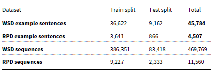
The WSD dataset includes sentences with one target word, annotated with its sense and part-of-speech, leveraging examples from the Chinese Wordnet 2.0 (CWN); Table 1 shows an example of the sense structure in CWN. The sense inventory of CWN provides fine-grained distinctions, with some words having more than 20 senses, yet the example sentences in CWN may fail to fully represent collocation environments for these complex words. To address this, manual sense annotation was performed in Hsieh et al. (Reference Hsieh, Tseng, Chou, Yang and Chang2024) for 113 words with more than 10 senses, using 27,012 sentences extracted from the ASBC. Sentences were filtered to exclude certain uses, such as proper nouns, transliterations, or segmentation errors. Six trained annotators, using a web-based tool, categorized the senses into hierarchical trees with an average depth of 2.77. The final annotation dataset comprises 28,836 examples in which the frequently used senses dominate, and only 57% of the senses are observed. Combined with CWN-derived data, the WSD dataset totals 45,784 examples, shown in the first row of Table 2. The dataset has a skewed sense distribution (see Appendix A), with more frequent senses making up a substantial portion of the data, ensuring a comprehensive representation of common polysemy.
Example sense structure of CWN with translation

Dataset statistics. The sequences are derived from the example sentences

3.2 RPD dataset
First, we differentiate between the concepts of dot object and type class to provide clarity on their roles in modeling regular polysemy. A dot object is a theoretical construct that represents systematic polysemous relationships in language, showing how a word or entity can carry multiple interrelated meanings. For example, the dot object “Producer.Product.Location reflects the different meanings of Starbucks” and alike, which can refer to an organization, a product, or a location. A type class, however, is a practical, context-specific application of a dot object that serves as a categorical label used in computational tasks to annotate and disambiguate the meaning of a term in its given context. For instance, “Starbucks” may be labeled as one of the three type classes (i.e., producer, product, or location) depending on its context. While dot objects offer the theoretical framework, type classes apply this framework in computational tasks.
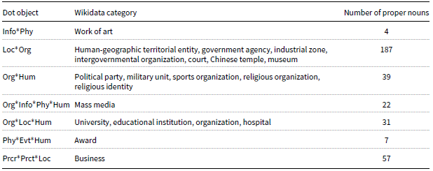
Dot objects mapped to Wikidata categories with the number of proper nouns in the dataset

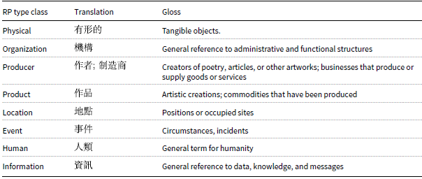
Regular polysemy type class with Mandarin translation and its gloss

The RPD dataset focuses on proper nouns identified as regularly polysemous within the corpus. It contains 4,507 example sentences sourced from the PTT Corpus, as indicated in the second row of Table 2. In total, 347 proper nouns are included, each appearing in one or more sentences. The proper nouns are annotated with one of seven predefined dot objects,Footnote e which capture systematic sense alternations observed in these entities. Table 3 presents the seven dot objects and their corresponding semantic categories, aligned with Wikidata entries as detailed by Hsieh et al. (Reference Hsieh, Tseng, Chou, Yang and Chang2024). Each instance of a proper noun in a specific sentence is assigned a type class based on its contextual meaning. The type classes involved in this dataset are shown in Table 4.
3.3 Model input
In the Transformer architecture, encoder-based models focus mainly on the encoder component, which is designed to process and encode input text into rich contextual representations by capturing bidirectional dependencies. These models are called encoder-based because they emphasize understanding and transforming the input into a meaningful representation for tasks like classification, named entity recognition, and question answering. On the other hand, decoder-based models utilize only the decoder component of the Transformer. The decoder is designed for autoregressive processing, generating text sequentially while attending to previous outputs, making these models ideal for tasks like text generation, summarization, and translation.
For the preparation of input data for different model types, we construct the input sequences of the models as context–gloss pairs. For encoder-based models, each test sentence $ t_i$
in the WSD dataset contains a predefined target word
$ t_i$
in the WSD dataset contains a predefined target word $ w_i$
, which is linked to a sense inventory provided by CWN. For each
$ w_i$
, which is linked to a sense inventory provided by CWN. For each $ t_i$
, we create
$ t_i$
, we create $ j$
input sequences, where
$ j$
input sequences, where $ j$
represents the number of senses of
$ j$
represents the number of senses of $ w_i$
(i.e., each input sequence corresponds to a specific sense
$ w_i$
(i.e., each input sequence corresponds to a specific sense $ s_{ij}$
of the target word). The sense
$ s_{ij}$
of the target word). The sense $ s_{ij}$
is described using its definition (SENSE-DEF) and an example sentence (SENSE-EX-SENT) from CWN. These components are combined with the original test sentence
$ s_{ij}$
is described using its definition (SENSE-DEF) and an example sentence (SENSE-EX-SENT) from CWN. These components are combined with the original test sentence $ t_i$
to construct the final input sequence as follows:
$ t_i$
to construct the final input sequence as follows:
 \begin{equation*} [\texttt {CLS}] \, \overbrace {\texttt {TEST-SENT}}^{t_i} \, [\texttt {SEP}] \, \overbrace {\texttt {TGT}}^{w_i}: \underbrace {\texttt {SENSE-DEF, SENSE-EX-SENT}}_{s_{ij}} \, [\texttt {SEP}] \end{equation*}
Thus, each test sentence generates as many sequences as there are senses in the inventory, with only one labeled correct (True). Target words having fewer than two predefined senses are excluded. For example, if a target word  (“case”) has three candidate senses, three sequences will be generated, as shown in Table 5. The total number of generated sequences is 469,769 as shown in the third row of Table 2. When POS hints are available, they are used as a filtering mechanism to constrain the candidate sense inventory prior to classification. Specifically, only candidate senses whose POS tag matches the annotated POS of the target word are retained as valid candidates. This reduces the number of input sequences generated per test sentence and eliminates cross-POS sense confusion. When no POS hint is provided, all senses in the inventory are included as candidates regardless of their POS tag.
The three model input sequences generated for  (“case”) for WSD. Each instance is represented with its translation below; only the instance in Taiwan Mandarin is used as the model input. When a POS hint is provided (as in the ”By example (POS)” evaluation), candidate senses whose POS tag does not match the target word’s annotated POS are excluded from the input sequences, resulting in fewer sequences per test sentence

For the RPD dataset, the input sequences are constructed in a similar way. Each test sentence $ t_i$
contains a single target word
$ t_i$
contains a single target word $ w_i$
, with its predefined RP-class inventory
$ w_i$
, with its predefined RP-class inventory $ rpclass\_inv_i$
retrieved. For each type class
$ rpclass\_inv_i$
retrieved. For each type class $ c_{ij}$ $\in$
$\in$ $ rpclass\_inv_i$
, its corresponding gloss (RPCLASS-GLOSS) is derived from the Revised Mandarin Chinese Dictionary. The input sequence is then concatenated as:
$ rpclass\_inv_i$
, its corresponding gloss (RPCLASS-GLOSS) is derived from the Revised Mandarin Chinese Dictionary. The input sequence is then concatenated as:
 \begin{equation*} [\texttt {CLS}] \, \overbrace {\texttt {TEST-SENT}}^{t_i} \, [\texttt {SEP}] \, \overbrace {\texttt {TGT}}^{w_i}: \underbrace {\texttt {RPCLASS, RPCLASS-GLOSS}}_{c_{ij}} \, [\texttt {SEP}] \end{equation*}
Each test sentence generates as many sequences as there are type classes in the inventory, with only one labeled correct (True). The target words are marked with angular brackets (i.e., $\mathtt {\lt \gt }$
) as a weak supervision signal. For example, if a target word
$\mathtt {\lt \gt }$
) as a weak supervision signal. For example, if a target word  (“Harvard”) has three candidate type classes, three sequences will be generated, as shown in Table 6. The total number of the generated sequences is 11,560, as shown in the last row in Table 2.
The three model input sequences generated for  (“Harvard”) for RPD. Each instance is represented with its translation below; only the instance in Taiwan Mandarin is used as the model input

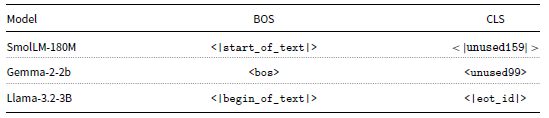
For decoder-based models, the input is slightly different because [CLS] and [SEP] tokens are not natively used. However, to more closely match the input used by encoder-based models, we designate other tokens to perform equivalent roles. To construct the input for a decoder-based model, we use the predefined beginning-of-sequence ([BOS]) token for the respective model to signal the beginning of an input and to serve as the delimiter token that separates the first sequence from the second. We then utilize an unused token from the vocabulary, such as $\mathtt {\lt unused99\gt }$
(token ID 255199) for Gemma-2-2b, to serve as the [CLS] token, indicating the end of the input sequence and providing the representation for the classification head. The input for the WSD task is structured as follows:
$\mathtt {\lt unused99\gt }$
(token ID 255199) for Gemma-2-2b, to serve as the [CLS] token, indicating the end of the input sequence and providing the representation for the classification head. The input for the WSD task is structured as follows:
 \begin{equation*} [\texttt {BOS}] \, \overbrace {\texttt {TEST-SENT}}^{t_i} \, [\texttt {BOS}] \, \overbrace {\texttt {TGT}}^{w_i}: \underbrace {\texttt {SENSE-DEF, SENSE-EX-SENT}}_{s_{ij}} \, [\texttt {CLS}] \end{equation*}
Similarly, the input for the RPD task is structured as follows:
 \begin{equation*} [\texttt {BOS}] \, \overbrace {\texttt {TEST-SENT}}^{t_i} \, [\texttt {BOS}] \, \overbrace {\texttt {TGT}}^{w_i}: \underbrace {\texttt {RPCLASS, RPCLASS-GLOSS}}_{c_{ij}} \, [\texttt {CLS}] \end{equation*}
The actual tokens used for each decoder-based model can be found in Appendix B.
It is worth noting a limitation of the current input design. By appending the target word and candidate sense definition after the test sentence, both encoder- and decoder-based models have access to the full sentential context (both preceding and subsequent). This effectively neutralizes one of the key architectural differences between the two model types: while encoders are inherently bidirectional, decoders are designed to attend only to preceding context. The current setup inadvertently grants decoder-based models access to subsequent context, providing them with an additional advantage that would not exist in a purely autoregressive setting.
3.4 Models and training details
3.4.1 Models
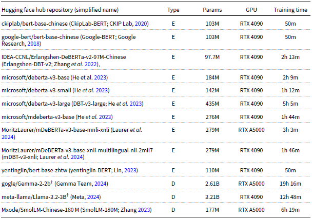
To evaluate the impact of model architecture on performance, we select a diverse range of encoder-based models, from Google’s original BERT (Devlin et al. Reference Devlin, Chang, Lee and Toutanova2019) to newer architectures, such as Microsoft’s DeBERTa (He, Gao, and Chen Reference He, Gao and Chen2023). The encoder-based models range in size from 97.7M to 435 M parameters, while the decoder-based models range from 177 M to 3.21B parameters. The largest decoder-based model is more than an order of magnitude larger than the smallest encoder-based model. A list of all models used can be found in Appendix C. To enhance readability and facilitate discussion, we will refer to these models using their abbreviated namesFootnote f in all subsequent sections. To use both encoder- and decoder-based models for classification, we utilize Transformers’ (Wolf et al. Reference Wolf, Debut, Sanh, Chaumond, Delangue, Moi, Cistac, Ma, Jernite, Plu, Xu, Scao, Gugger, Drame, Lhoest and Rush2020) AutoModelForSequenceClassification, which allows us to easily add a classifier head with two output neurons, corresponding to the False and True classes. The respective [CLS] token for each model is fed into the classifier head to make a prediction.
3.4.2 Training details
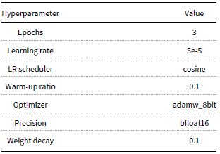
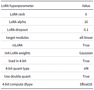
We fine-tune all models using the Hugging Face Transformers (v. 4.46.3) Trainer. We perform full-parameter fine-tuning for all encoder-based models and the SmolLM-180M decoder-based model. For the larger decoder-based models, Gemma-2-2b and Llama-3.2-3B, we use Low-Rank Adaptation (LoRA) (Hu et al. Reference Hu, Shen, Wallis, Allen-Zhu, Li, Wang, Wang and Chen2022) due to their size and memory requirements. The hyperparameters for full-parameter and LoRA fine-tuning can be found in Appendix D. All training was conducted on a single GPU with 24 GB of VRAM (either an Nvidia RTX 4090 or an Nvidia RTX A5000). We train for three epochs, saving a checkpoint after each epoch and select the checkpoint with the lowest cross-entropy evaluation loss.
3.4.3 Training times
The BERT base models had the shortest training times, all requiring approximately 50 minutes. Gemma-2-2b took the longest at 19 hours and 16 minutes, which is 23 times longer than the BERT models. Even the smallest decoder-based model, SmolLM-180M (177M parameters), required 6 hours and 19 minutes to train. In comparison, the encoder-based model with a similar number of parameters, deberta-v3-base (184M parameters), took only 2 hours and 9 minutes. Despite having more parameters, the encoder-based model trained in almost one-third of the time.
3.4.4 Carbon emission estimation details
Carbon emissions were estimated following Patterson et al. (Reference Patterson, Gonzalez, Holzle, Le, Liang, Munguia, Rothchild, So, Texier and Dean2022), with an explicit system overhead factor to separate GPU-measured energy from total server energy following Luccioni et al. (Reference Luccioni, Viguier and Ligozat2023). GPU energy was measured via Weights & Biases using NVML hardware counters. A system overhead factor of $1.5\times$
was applied to account for non-GPU server power (CPU, memory, storage, fans), with PUE of 1.2 for on-premises infrastructure (NTU server room, Taiwan) and 1.3 for cloud infrastructure (RunPod, datacenter region unknown). Carbon intensity was 0.474 kgCO
$1.5\times$
was applied to account for non-GPU server power (CPU, memory, storage, fans), with PUE of 1.2 for on-premises infrastructure (NTU server room, Taiwan) and 1.3 for cloud infrastructure (RunPod, datacenter region unknown). Carbon intensity was 0.474 kgCO $_2$
eq/kWh for on-premises compute (Energy Administration, Ministry of Economic Affairs, 2024) and 0.475 kgCO
$_2$
eq/kWh for on-premises compute (Energy Administration, Ministry of Economic Affairs, 2024) and 0.475 kgCO $_2$
eq/kWh (conservative upper bound) for cloud compute. Results are reported in Table 10; for a comparative review of carbon estimation approaches, see Bouza et al. (Reference Bouza, Bugeau and Lannelongue2023).
$_2$
eq/kWh (conservative upper bound) for cloud compute. Results are reported in Table 10; for a comparative review of carbon estimation approaches, see Bouza et al. (Reference Bouza, Bugeau and Lannelongue2023).
4. Results
4.1 Model performance on WSD
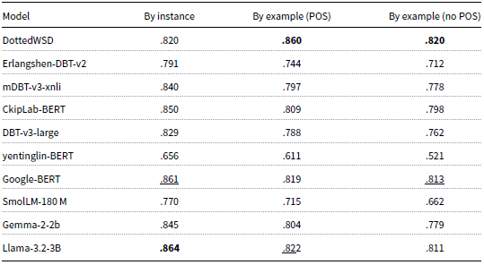
Table 7 shows the evaluation of the encoder- and decoder-based models on the WSD dataset. DottedWSD, constructed in the previous study, emerges as a strong baseline, achieving an accuracy of 82% by instance and 86% by example with POS hints.
Model accuracy in WSD. Bold numbers indicate the best accuracy, while numbers with a double underline indicate the second-best accuracy. For clarity, only the best model among the same family is listed; for example, DBT-v3-large is listed among the deberta-v3 family. The accuracy of all models is shown in Figure 1

Model accuracy on WSD (by example) with POS hints. The yellow bars represent the encoder-based models and the green bars represent the decoder-based models.

Model accuracy on WSD (by example) without POS hints. The yellow bars represent the encoder-based models and the green bars represent the decoder-based models.

Llama-3.2-3B achieves the highest accuracy by instance (.864), outperforming the other models. In particular, it also excels in by-example evaluations with POS (.821) and without POS (.811), closely followed by the performance of Google-BERT by instance (.861) and by example (.818 and .813). Notably, Llama-3.2-3B is a decoder-based model, while Google-BERT is an encoder-based model.
Lower-performing models, such as yentinglin-BERT (.656) and SmolLM-180M (.770), highlight the challenges faced by models with limited scale or pretraining resources. The performance gap underscores the importance of incorporating high-quality large-scale data that capture linguistic nuances and domain-specific lexical variations.
The comparison between Figures 1 and 2 illustrates that the introduction of POS hints generally enhances performance in most models, highlighting their role in providing additional syntactic context. This aligns with the findings of Hsieh et al. (Reference Hsieh, Tseng, Chou, Yang and Chang2024), which suggest that while POS hints yield modest improvements, the models primarily rely on distinguishing lexical semantics rather than heavily depending on POS tags. The trend is more obvious for mid-performing models, such as SmolLM-180M, which benefit significantly from the POS hints. In contrast, high-performing models, such as Google-BERT and Llama-3.2-3B, demonstrate marginal improvements, suggesting that these models may already integrate sufficient contextual and syntactic information during prediction.
A particularly revealing comparison emerges between SmolLM-180 M (177M parameters) and deberta-v3-base (184M parameters), two models of comparable size but different architectures. Despite having a similar parameter count, deberta-v3-base achieves a substantially higher accuracy by instance (.840) compared to SmolLM-180 M (.770), representing a gap of 7 percentage points. This suggests that the encoder architecture holds an inherent advantage over the decoder architecture when model size is controlled for. In light of this, the comparable performance of Llama-3.2-3B (.864) relative to Google-BERT (.861) should be interpreted with caution – the similarity in their scores likely reflects the decoder model’s significantly larger parameter count (3.21B vs. 103M) and more extensive pretraining data, rather than architectural equivalence. These findings further reinforce the argument that encoder-based models can achieve competitive performance at a substantially lower model scale.
When interpreting these results, it should be noted that the input design described in Section 3.3 may partially favor decoder-based models. Since the candidate sense definitions are appended after the test sentence, decoders can attend to the full context rather than only the preceding tokens. This means the performance gap between encoder- and decoder-based models may be underestimated, and encoder-based models may in fact hold a greater advantage under a more naturalistic autoregressive setting.
4.2 Model performance on RPD task
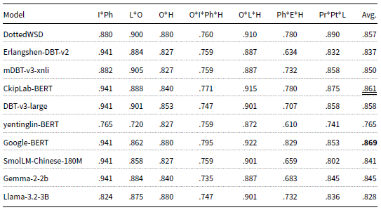
Table 8 shows the evaluation of the model accuracy when disambiguating regular polysemy. The results highlight distinctions in how encoder- and decoder-based models handle semantic alternation in proper nouns.
Model accuracy on RPD task. The type classes are abbreviated with their initials: I: Information, Ph: Physical, L: Location, H: Human, O: Organization, E: Event, Pr: Producer, Pt: Product. The bold number indicates the best accuracy, while the number with a double underline indicates the second-best accuracy

Table 8. Long description
The table presents the evaluation of model accuracy in disambiguating regular polysemy, with a focus on how encoder- and decoder-based models handle semantic alternation in proper nouns. The table has 10 rows and 10 columns, including the model names and their accuracy scores across different type classes. The type classes are abbreviated with their initials: I for Information, Ph for Physical, L for Location, H for Human, O for Organization, E for Event, Pr for Producer, and Pt for Product. The accuracy scores are provided for each model across these type classes. The bold number indicates the best accuracy, while the number with a double underline indicates the second-best accuracy. Row 1: Dotted WSD, I Ph: 0.880, L: 0.900, O H: 0.880, O Pt: 0.760, Ph H: 0.910, O L H: 0.780, Ph E H: 0.890, Pr Pt: 0.850, L: 0.857. Row 2: Erlangshen-DBT-v2, I Ph: 0.941, L: 0.884, O H: 0.827, O Pt: 0.759, Ph H: 0.887, O L H: 0.634, Ph E H: 0.832, Pr Pt: 0.837, L: 0.837. Row 3: mDBT-v3-xnli, I Ph: 0.882, L: 0.905, O H: 0.827, O Pt: 0.759, Ph H: 0.887, O L H: 0.732, Ph E H: 0.858, Pr Pt: 0.850, L: 0.850. Row 4: CkipLab-BERT, I Ph: 0.941, L: 0.888, O H: 0.840, O Pt: 0.771, Ph H: 0.915, O L H: 0.780, Ph E H: 0.875, Pr Pt: 0.861, L: 0.861. Row 5: DBT-v3-large, I Ph: 0.941, L: 0.901, O H: 0.853, O Pt: 0.747, Ph H: 0.901, O L H: 0.707, Ph E H: 0.858, Pr Pt: 0.858, L: 0.858. Row 6: Yentinglin-BERT, I Ph: 0.765, L: 0.720, O H: 0.827, O Pt: 0.759, Ph H: 0.872, O L H: 0.610, Ph E H: 0.741, Pr Pt: 0.765, L: 0.765. Row 7: Google-BERT, I Ph: 0.941, L: 0.862, O H: 0.880, O Pt: 0.795, Ph H: 0.922, O L H: 0.829, Ph E H: 0.853, Pr Pt: 0.869, L: 0.869. Row 8: SmolLM-Chinese-180M, I Ph: 0.941, L: 0.858, O H: 0.827, O Pt: 0.759, Ph H: 0.901, O L H: 0.659, Ph E H: 0.802, Pr Pt: 0.841, L: 0.841. Row 9: Gemma-2-2b, I Ph: 0.941, L: 0.884, O H: 0.840, O Pt: 0.735, Ph H: 0.887, O L H: 0.683, Ph E H: 0.845, Pr Pt: 0.845, L: 0.845. Row 10: Llama-3-2-3B, I Ph: 0.824, L: 0.875, O H: 0.880, O Pt: 0.747, Ph H: 0.901, O L H: 0.732, Ph E H: 0.836, Pr Pt: 0.828, L: 0.828.
Comparison of average model accuracy on WSD and RPD between encoder-based and decoder-based models

Google-BERT outperforms other models with an average accuracy of .869, indicating its robust handling of systematic sense alternations such as Location*Organization and Organization*Human. This superior performance may be attributed to its extensive multilingual and domain-specific pretraining. Interestingly, CkipLab-BERT, trained by the CKIP Lab located in Taiwan, achieves an average accuracy of .861, outperforming several larger models. This result underscores the importance of pretraining strategies tailored to the linguistic and cultural nuances of the target language, especially for tasks that involve named entities with culture-specific usage patterns.
The variation in performance across dot-type categories, such as Information*Physical and Producer*Product*Location, suggests that the models are sensitive to the complexity of class overlaps. For example, models generally struggle more with overlapping categories like Physical*Event*Human compared to more distinct classes like Location*Organization, where contextual cues may be clearer.
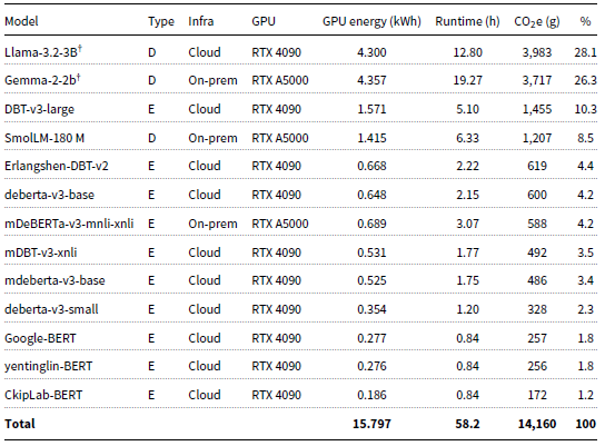
Training carbon emissions for all 13 runs (1 run = WSD + RPD task). CO $_2$
e is computed following the method described in Section 3.4.4, with
$_2$
e is computed following the method described in Section 3.4.4, with $f_{\text{sys}} = 1.5$
, PUE of 1.2 (on-premises) and 1.3 (cloud), and carbon intensity of 0.474 kgCO
$f_{\text{sys}} = 1.5$
, PUE of 1.2 (on-premises) and 1.3 (cloud), and carbon intensity of 0.474 kgCO $_2$
eq/kWh (on-premises) and 0.475 kgCO
$_2$
eq/kWh (on-premises) and 0.475 kgCO $_2$
eq/kWh (cloud). GPU energy is derived from NVML power samples logged via Weights & Biases. Type: E = encoder, D = decoder.
$_2$
eq/kWh (cloud). GPU energy is derived from NVML power samples logged via Weights & Biases. Type: E = encoder, D = decoder. $\dagger$
= trained with LoRA
$\dagger$
= trained with LoRA

In summary, Table 9 illustrates the comparable performance of encoder- and decoder-based models on WSD and RPD tasks. The average WSD accuracy is closely aligned, with encoders achieving 77.5% and decoder-based models performing slightly better at 78.5%. For the RPD task, encoder-based models achieve a higher average score of 84.2 %, compared to 83.8 % for decoder-based models. However, these aggregate figures obscure an important architectural difference. The near-equivalent performance of the two model types is largely driven by the inclusion of Llama-3.2-3B, a model with 3.21B parameters – over 31 times larger than the best-performing encoder model, Google-BERT (103M parameters). When comparing models of similar scale, such as SmolLM-180 M (177M parameters) and deberta-v3-base (184M parameters), the encoder-based model clearly outperforms its decoder counterpart (84.0 % vs. 77.0 % by instance). This size-controlled comparison strengthens the case for encoder-based models as a more parameter-efficient choice for WSD and RPD tasks and provides a basis for further exploration of their efficiency and sustainability.
4.3 Training carbon emissions by architecture
Table 10 reports training energy consumption and estimated CO $_2$
e emissions for all 13 runs (1 run = WSD + RPD task). In total, training consumed 15.8 kWh of GPU energy across 58.2 GPU-hours, producing an estimated 14.2 kg CO
$_2$
e emissions for all 13 runs (1 run = WSD + RPD task). In total, training consumed 15.8 kWh of GPU energy across 58.2 GPU-hours, producing an estimated 14.2 kg CO $_2$
e under the central scenario (see Section 3.4.4). A sensitivity analysis over overhead assumptions yields a lower bound of 7.5 kg (GPU energy only, no system or facility overhead) and an upper bound of 17.5 kg (HPC-scale
$_2$
e under the central scenario (see Section 3.4.4). A sensitivity analysis over overhead assumptions yields a lower bound of 7.5 kg (GPU energy only, no system or facility overhead) and an upper bound of 17.5 kg (HPC-scale $f_{\text{sys}} = 1.85$
, as reported for the BLOOM training cluster). The three decoder-based models (Llama-3.2-3B, Gemma-2-2b, SmolLM-180M) accounted for 62.9% of total emissions despite comprising only 3 of 13 runs. This reflects the substantially higher compute cost of autoregressive fine-tuning: decoder models generate output token-by-token and must process the full sequence at each step, whereas encoder models perform a single forward pass over the entire input. The emissions asymmetry is particularly evident in the size-controlled comparison between SmolLM-180 M (177M parameters, decoder) and deberta-v3-base (184M parameters, encoder): despite near-identical parameter counts, SmolLM-180 M produced 1,207 g CO
$f_{\text{sys}} = 1.85$
, as reported for the BLOOM training cluster). The three decoder-based models (Llama-3.2-3B, Gemma-2-2b, SmolLM-180M) accounted for 62.9% of total emissions despite comprising only 3 of 13 runs. This reflects the substantially higher compute cost of autoregressive fine-tuning: decoder models generate output token-by-token and must process the full sequence at each step, whereas encoder models perform a single forward pass over the entire input. The emissions asymmetry is particularly evident in the size-controlled comparison between SmolLM-180 M (177M parameters, decoder) and deberta-v3-base (184M parameters, encoder): despite near-identical parameter counts, SmolLM-180 M produced 1,207 g CO $_2$
e compared to 600 g for deberta-v3-base – less than half the emissions for a comparable model scale.
$_2$
e compared to 600 g for deberta-v3-base – less than half the emissions for a comparable model scale.
5. Large-scale all-words sense tagging task
Building on the results of our initial experiment, which has revealed that encoder- and decoder-based models exhibit comparable performance on WSD and RPD tasks, as illustrated in Table 9, we investigate the efficiency and sustainability of these models further, particularly regarding energy consumption and carbon emissions. We conduct a second experiment centered on large-scale, all-words sense tagging using data from the ASBC. This experiment focuses on two high-performing models, Google-BERT and Llama-3.2-3B, to perform a detailed evaluation of their sense tagging capabilities. The aim is to assess their scalability on larger datasets and explore the implications for designing environmentally sustainable models while enhancing the accessibility of lexical resources for wider use.
5.1 Data and model configuration
Each line within the ASBC is processed to identify words with multiple potential senses according to their corresponding sense inventory. This results in a total of 32.7 million instances. The transformation of the model input follows the procedure for creating training and testing data in Section 3.3, where the complete sentence containing the target word TGT is represented as TEST-SENT, the sense definition as SENSE-DEF, and one example sentence for the given sense as SENSE-EX-SENT. The input structure of the encoder-based models is defined as:
 \begin{equation*} [\texttt {CLS}] \, \texttt {TEST-SENT} \, [\texttt {SEP}] \, \texttt {TGT, SENSE-DEF, SENSE-EX-SENT} \, [\texttt {SEP}] \end{equation*}
In contrast, the decoder-based model input structure is given as:
 \begin{equation*} [\texttt {BOS}] \, \texttt {TEST-SENT} \, [\texttt {BOS}] \, \texttt {TGT, SENSE-DEF, SENSE-EX-SENT} \, [\texttt {CLS}] \end{equation*}
Model inference was conducted using both Google-BERT and Llama-3.2-3B. Google-BERT inference is performed on a single Nvidia A5000 GPU with 24 GB of VRAM, requiring approximately 17 hours. To expedite the process for Llama-3.2-3B, inference is distributed across 6 Nvidia A40 GPUs, each with 48 GB of VRAM, totaling 288 GB. This distributed approach results in a total inference time of 126 GPU hours.
5.2 Results and discussion
Table 11 shows that Google-BERT slightly outperforms Llama-3.2-3B in the sense tagging accuracy (94.5% vs. 92.5 %). This suggests that the encoder-based architecture of BERT is well suited for the WSD task in Taiwan Mandarin. The annotation agreement between the two models, measured using Cohen’s Kappa, is moderate at 0.664, indicating substantial but incomplete alignment in their outputs.
Comparison of model accuracy, GPU resources, total GPU hours, and estimated carbon emissions produced on the all-words sense tagging task. Carbon emissions follow the estimation method in Section 3.4.4; the A40 inference run uses the cloud PUE and carbon-intensity values defined there.

Not only does Google-BERT excel in performance, it also shows to be significantly more resource efficient. The model requires only a single GPU and completes inference in 17 hours, producing an estimated 1.69 kg CO $_{2}$
eq. In comparison, the larger decoder-based model, Llama-3.2-3B, necessitates distributed inference across six GPUs to complete within a reasonable time frame, in a total computational cost of 126 GPU hours and an estimated 13.61 kg CO
$_{2}$
eq. In comparison, the larger decoder-based model, Llama-3.2-3B, necessitates distributed inference across six GPUs to complete within a reasonable time frame, in a total computational cost of 126 GPU hours and an estimated 13.61 kg CO $_{2}$
eq, which is approximately eight times the carbon footprint of Google-BERT. This distinction is crucial for deploying NLP technologies in an eco-friendly manner. In other words, Google-BERT achieves comparable results compared to Llama-3.2-3B with a significantly smaller resource footprint. This highlights a key trade-off between model size and computational cost. Although decoder-based models are powerful, their substantial resource demands may not be justifiable in tasks where encoder-based models achieve similar performance.
$_{2}$
eq, which is approximately eight times the carbon footprint of Google-BERT. This distinction is crucial for deploying NLP technologies in an eco-friendly manner. In other words, Google-BERT achieves comparable results compared to Llama-3.2-3B with a significantly smaller resource footprint. This highlights a key trade-off between model size and computational cost. Although decoder-based models are powerful, their substantial resource demands may not be justifiable in tasks where encoder-based models achieve similar performance.
These findings contribute to ongoing discussions in the NLP community to prioritize sustainability in model development. A key consideration is the integration of energy consumption and computational cost metrics into existing evaluation frameworks. As emphasized in prior work (Strubell, Ganesh, and McCallum Reference Strubell, Ganesh and McCallum2019; Castaño et al. Reference Castaño, Martínez-Fernández, Franch and Bogner2023), selecting and designing models that balance performance with environmental responsibility is essential. Recent automated tracking tools such as CodeCarbon (Schmidt et al. Reference Schmidt, Goyal, Joshi, Feld, Conell, Laskaris, Blank, Wilson, Friedler and Luccioni2021) and Carbontracker (Anthony, Kanding, and Selvan Reference Anthony, Kanding and Selvan2020) have made per-experiment emissions monitoring increasingly accessible, lowering the barrier to systematic carbon reporting in NLP research. Practical measures, such as adopting lighter models and faster GPUs (Liu and Yin Reference Liu and Yin2024), offer a promising way to reduce the carbon footprint of large-scale language models while maintaining robust model performance. Furthermore, establishing standardized frameworks for measuring and reporting the environmental impact of NLP systems, such as the Digital and Green Index (DGI) (Thelisson et al. Reference Thelisson, Mika, Schneiter, Padh and Verma2023), is crucial for fostering transparency and accountability within the field. By incorporating metrics such as energy efficiency, carbon emissions, and GPU utilization into existing benchmarks, a more comprehensive evaluation of models becomes possible, considering both their technical capabilities and their environmental footprint. Such steps not only align with the growing demand for responsible AI development but contribute to broader sustainability goals, including the United Nations Sustainable Development Goal 13 (SDG 13) (Louman et al. Reference Louman, Keenan, Kleinschmit, Atmadja, Sitoe, Nhantumbo, de Camino Velozo and Morales2019) on climate action. By integrating these considerations into the core of NLP research practices, the field can ensure that technological advancements are both impactful and environmentally conscious.
6. Conclusion
This study provides an assessment of encoder- and decoder-based models for WSD and RPD of proper nouns, using datasets from the CWN and two corpora in Taiwan Mandarin. Encoder-based models not only deliver comparable accuracy to decoders on WSD tasks, but they also exhibit greater computational efficiency. In contrast, decoder-based models, despite their higher resource requirements, perform worse than encoders on RPD tasks. The findings emphasize seeking balance among model performance, resource consumption, and environmental considerations. This highlights the importance of selecting models based on task-specific needs and resource constraints.
The implications of these findings extend beyond Taiwan Mandarin to other low-resource languages and multilingual NLP settings. Many languages lack the large annotated corpora and computational resources required to fine-tune and deploy large decoder-based models. Our results suggest that encoder-based models, which achieve comparable or superior performance at a fraction of the computational cost, represent a more practical and sustainable choice for such settings. This is particularly relevant for languages where lexical resources such as wordnets or sense inventories exist but training data remains scarce. By demonstrating that smaller, encoder-based models can match the performance of significantly larger decoders on fine-grained semantic tasks, this study provides a compelling case for prioritizing efficient architectures in the development of NLP tools for underrepresented languages. Furthermore, the substantially lower carbon footprint of encoder-based models aligns with the broader goal of democratizing NLP research, enabling institutions with limited resources, including those in developing regions, to conduct meaningful research without incurring prohibitive computational costs.
This study highlights the importance of considering both accuracy and resource consumption when selecting model architectures, particularly as large-scale models are increasingly being deployed. Future work should focus on optimizing models to achieve a balance between performance and efficiency, exploring techniques to minimize energy consumption while maintaining task accuracy. Integrating standardized sustainability metrics into evaluation frameworks is crucial to advancing environmentally conscious language models. The growing ecosystem of dedicated tracking tools offers a concrete path toward reproducible carbon reporting as a routine component of NLP benchmarking. This study demonstrates encoder-based models as being not only computationally efficient but also potentially less energy-intensive, advocating the use of smaller, task-focused, and sustainable models to reduce the environmental footprint of NLP systems.
Acknowledgments
The authors used AI language tools (ChatGPT, Gemini, and Claude) to assist with analysis scripts and light editorial revision of draft text. All scientific content, analysis, and conclusions are the authors’ own.
Appendix A. Sense distribution in CWN

Appendix B. Decoder-based model input structure
The special tokens used for decoder-based models. BOS is used at the beginning of an example and to separate the first and second sequences. CLS indicates the end of the example. The model uses CLS as input for the classifier head

Appendix C. Models used
All models were trained on one GPU (24 GB VRAM) either locally or through a cloud GPU provider. Type refers to if the model is an encoder (E) or a decoder (D) model.

Table C1. Long description
The table contains information about different models trained on one GPU. It has 13 rows and 4 columns. The columns are Hugging face hub repository (simplified name), Type, Params, GPU, and Training time. Row 1: ckiplab/bert-base-chinese (CkipLab-BERT), E, 103M, RTX 4090, 50m. Row 2: google-bert/bert-base-chinese (Google-BERT), E, 103M, RTX 4090, 50m. Row 3: IDEA-CCNL/Erlangshen-DeBERTa-v2-97M-Chinese (Erlangshen-DBT-v2), E, 97.7M, RTX 4090, 2h 13m. Row 4: microsoft/deberta-v3-base, E, 184M, RTX 4090, 2h 9m. Row 5: microsoft/deberta-v3-small, E, 142M, RTX 4090, 1h 12m. Row 6: microsoft/deberta-v3-large (DBT-v3-large), E, 435M, RTX 4090, 5h 5m. Row 7: microsoft/mdeberta-v3-base, E, 276M, RTX 4090, 1h 44m. Row 8: MoritzLaurer/mDeBERTa-v3-base-mnli-xnli, E, 279M, RTX A5000, 3h 3m. Row 9: MoritzLaurer/mDeBERTa-v3-base-xnli-multilingual-nli-2mil7 (mDBT-v3-xnli), E, 279M, RTX 4090, 1h 46m. Row 10: yentinglin/bert-base-zhtw (yentinglin-BERT), E, 110M, RTX 4090, 50m. Row 11: google/Gemma-2-2b, D, 2.61B, RTX A5000, 19h 16m. Row 12: meta-llama/Llama-3.2-3B, D, 3.21B, RTX 4090, 12h 48m. Row 13: Mxode/SmolLM-Chinese-180 M (SmolLM-180M), D, 177M, RTX A5000, 6h 19m.
† indicates the model was trained using LoRA. This table contains all models that were trained. The results presented in the main text only present the model with the best performance within a family of models (e.g., only Microsoft’s DBT-v3-large is present when there are actually small, base, and large variants
Appendix D. Hyperparameters
The hyperparameters used to train the majority models with Transformers’ Trainer. Note: Mxode/SmolLM-Chinese-180M was trained in FP32 because of training instability when using BF16

The LoRA hyperparameters used to train Llama-3.2-3B and google-Gemma-2-2b

 . Technical report,
  ). Available at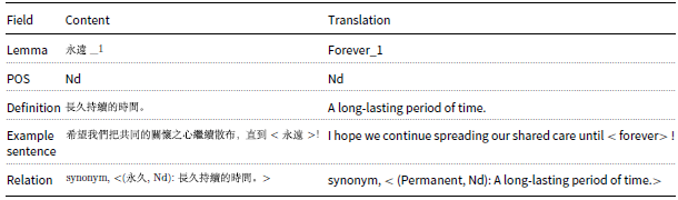









 Open access

