


1. Introduction
Laminar–turbulent transition of supersonic boundary-layer flows has been regarded as one of the most challenging problems in the design and optimisation of many aerodynamic configurations. Accurate prediction of transition has immense practical importance because a drastic increase of skin friction and heat transfer will occur when the flow changes from its laminar state to turbulence (Fedorov Reference Fedorov2011; Schneider 2015). This complex physical process involves several stages: receptivity (Goldstein & Hultgren Reference Goldstein and Hultgren1989), linear amplification of instability modes, nonlinear inter-modal interactions and final breakdown to random motions (Kachanov Reference Kachanov1994; Wu 2019). While transition is underpinned by internal dynamics, i.e. intrinsic instabilities, of the flow, it is also known to be affected strongly by external disturbances in the free stream and/or on the body surface (Schneider 2001). In particular, ambient acoustic waves play a crucial role in transition of supersonic boundary layers (Pate & Schueler Reference Pate and Schueler1969; Schneider 2001). To gain a deep understanding of the underlying flow physics, we study the evolution of instability waves in a supersonic boundary layer under the influence of impinging sound waves, with the goal to identify mechanisms through which the latter affects linear and nonlinear development of the former.
1.1. Subharmonic resonance of intrinsic instabilities
Subharmonic resonance is a common nonlinear wave phenomenon. In particular, subharmonic resonance of instability modes has been proposed as an important nonlinear process causing boundary-layer transition. It involves triadic interactions between a plane wave and a pair of symmetrical oblique waves, the latter having subharmonic frequency and streamwise wavenumber half of that of the former. Existence of such a triad of Tollmien–Schlichting (T-S) modes in the Blasius boundary layer was noted by Raetz (1959), and a heuristic theoretical description, put forward by Craik (Reference Craik1971) on the basis of finite Reynolds number, showed that the resonance leads to continual energy transfer between the mean flow and the disturbance, energising the oblique modes especially. Kachanov & Levchenko (Reference Kachanov and Levchenko1984) and Saric & Thomas (1984) performed controlled experiments and observed rapid growth of the oblique subharmonics. Prompted by these experiments, Smith & Stewart (1987) studied the resonant-triad interaction of T-S waves in a Blasius boundary layer based on a high-Reynolds-number approach, showing that subharmonic triads of three nearly neutral modes always exist in the so-called high-frequency limit of the lower-branch regime. On noting that in experiments, subharmonic-resonance induced rapid growth occurred near the upper branch of the neutral curve, where a distinct critical layer arises, Mankbadi, Wu & Lee (Reference Mankbadi, Wu and Lee1993) and Wu (1993) presented asymptotic theories on the resonant triad in the upper-branch instability regime for the Blasius and the accelerating boundary layers, respectively. They showed that the dominant nonlinear interactions occur in the critical layer and the surrounding diffusion layer (cf. Smith & Stewart 1987). The oblique modes, typically having small amplitude initially, experience super-exponential growth through interaction with the planar mode at quadratic level, but the latter continues to amplify in accordance with linear stability theory without the feedback effect from the former. If the amplitude of the oblique modes is algebraically small, following the parametric resonance, the cubic interactions of the subharmonics suppress the growth (Wu 1993). If the oblique modes have an exponentially small initial amplitude, its rapid super-exponential growth leads to a fully coupled stage (Goldstein Reference Goldstein1994; Wu Reference Wu and Cowley1995; Wu et al. Reference Wu, Stewart, Cowley, Bonilla, Moscoso, Platero and Vega2008).
Resonant-triad interactions of long- and $O(1)$
-wavelength Rayleigh instabilities were studied by Goldstein & Lee (Reference Goldstein and Lee1992) and Wu (1992), respectively. Similar to the resonant triad of T-S modes, the development of the interacting Rayleigh waves starts with a parametric resonance stage when the initial size of the oblique modes is significantly smaller than that of the planar wave. In this stage, the subharmonic oblique waves undergo super-exponential amplification while the fundamental planar wave grows exponentially, playing the role of a catalyst (Wu et al. Reference Wu, Stewart, Cowley, Bonilla, Moscoso, Platero and Vega2008; Wu 2019). Owing to the continual fast growth of the oblique modes, the triad eventually enters a fully interactive regime. The evolution equations for the fully coupled triad were extended to the supersonic regime, where there exists a resonant triad consisting of a planar second Mack mode and a pair of oblique first modes (Al-Salman Reference Al-Salman2003).
$O(1)$
-wavelength Rayleigh instabilities were studied by Goldstein & Lee (Reference Goldstein and Lee1992) and Wu (1992), respectively. Similar to the resonant triad of T-S modes, the development of the interacting Rayleigh waves starts with a parametric resonance stage when the initial size of the oblique modes is significantly smaller than that of the planar wave. In this stage, the subharmonic oblique waves undergo super-exponential amplification while the fundamental planar wave grows exponentially, playing the role of a catalyst (Wu et al. Reference Wu, Stewart, Cowley, Bonilla, Moscoso, Platero and Vega2008; Wu 2019). Owing to the continual fast growth of the oblique modes, the triad eventually enters a fully interactive regime. The evolution equations for the fully coupled triad were extended to the supersonic regime, where there exists a resonant triad consisting of a planar second Mack mode and a pair of oblique first modes (Al-Salman Reference Al-Salman2003).
When the subharmonic modes in the triad become two-dimensional, the resonance takes in a simpler form between a planar fundamental and a planar subharmonic. Such a subharmonic resonance consisting of two Rayleigh instability modes was proposed as a mechanism explaining vortex pairing on mixing layers and jets (Monkewitz Reference Monkewitz1988). More generally, the two waves in resonance do not both have to be eigenmodes: one of them (e.g. the fundamental) may be externally imposed or sustained. Resonance in such a case is often referred to as Bragg scattering (Bragg Reference Bragg1913). An example is a water wave propagating in a layer of fluid over a spatially periodic topography (Mei Reference Mei1985; Mei, Hara & Naciri Reference Mei, Hara and Naciri1988). A similar resonance may take place between stationary cross-flow vortices and periodic-roughness-induced modes (He, Butler & Wu Reference He, Butler and Wu2019; Xu & Wu Reference Xu and Wu2022). As it will transpire, the subharmonic parametric resonance in the present work is akin to that in these studies, but the critical layer, where resonant interaction takes place, plays an important role as observed by Goldstein & Lee (Reference Goldstein and Lee1992) and Wu (Reference Wu and Cowley1995).
1.2. Role of acoustic disturbances in supersonic boundary-layer transition
Naturally present physical external disturbances that may have a substantial impact on transition consist of surface roughness elements, vortical disturbances and sound waves in the oncoming flow. Depending on their length/time scales, intensity and location, they may affect the transition route and position through a variety of mechanisms including receptivity, local scattering, participation in modal interaction, modification of linear stability characteristics and even induction of new instability. A survey of the role of roughness and vortical disturbances in these mechanisms was given by Qin & Wu (Reference Qin and Wu2024). Here, we focus on acoustic waves.
Acoustic waves represent a form of external disturbances that significantly influence supersonic boundary-layer transition, particularly in the context of conventional wind tunnel experiments (Schneider 2001), where intensive noise is emitted from turbulent boundary layers on the tunnel walls and/or radiated due to turbulence being scattered by wall inhomogeneities such as roughness elements (Laufer Reference Laufer1961, Reference Laufer1964). Numerous wind tunnel experiments have been conducted to characterise the relationship between noise levels and transition locations. In the case of a supersonic flat-plate boundary layer, a comparative analysis of transition measurements in nine distinct wind tunnels varying in diameter from 30 cm to 130 cm indicated that a reduction in noise intensity leads to an increase of the transition Reynolds number (Pate & Schueler Reference Pate and Schueler1969). This general trend was confirmed by a parallel investigation on a cone in six different hypersonic facilities at NASA Langley (Stainback 1971). By relaminarising the boundary layers on the tunnel walls to mitigate the acoustic radiation, a significant delay in transition was observed (Kendall Reference Kendall1971). The wind tunnel experiment conducted by Kendall (Reference Kendall1975) further elucidated intricate interplay between free stream facility noise and boundary-layer instability, revealing an increasingly pronounced impact of the noise as the Mach number progresses into the hypersonic regime.
Given the intense acoustic disturbances that test models are exposed to in conventional wind tunnels, the transition process differs notably from that observed in quieter environments (Beckwith & Miller Reference Beckwith and Miller1990; King Reference King1992; Schneider 2008). Modern hypersonic quiet wind tunnel technology aims to replicate flight conditions as closely as possible (Schneider 2015). Nevertheless, acoustic waves may still be radiated from engines or turbulent boundary layers over adjacent aircraft surfaces, potentially exerting a substantial impact on transition. In view of this, conventional tunnels share certain similarities with flight conditions, and the experimental data obtained from them regarding instability and transition may still provide valuable insights (Duan et al. Reference Duan, Choudhari and Wu2014, Reference Duan2019).
1.3. Scope of the present study
Our concern is with supersonic modes in compressible boundary layers. The existence of these modes is well known (Mack Reference Mack1984), and has been reported for various configurations including flows over flat plates (Mack Reference Mack, Dwoyer and Hussaini1987; Bitter & Shepherd Reference Bitter and Shepherd2015), wedges (Chang et al. Reference Chang, Malik and Hussaini1990, Reference Chang, Vinh and Malik1997) and cones (Knisely & Zhong Reference Knisely and Zhong2017; Mortensen Reference Mortensen2018). A prominent feature of the mode is that its eigenfunction is oscillatory while attenuating, or remains bounded in the far field when the mode is neutral. Sound radiation by supersonic modes in a hypersonic blunt-cone boundary layer was studied numerically by Knisely & Zhong (Reference Knisely and Zhong2019a ,Reference Knisely and Zhong b ), whereas the radiation by these modes in supersonic free shear layers and jets had been studied theoretically by Tam & Burton (Reference Tam and Burton1984a,b) and Wu (2005).
High-enthalpy impulse facilities have been designed to replicate flight conditions, but the detrimental effects are short test time and high levels of free stream noise. In such high-enthalpy environment, supersonic modes are found to exist if the wall is cooled sufficiently below the adiabatic temperature, and may become unstable over a wider frequency band than subsonic modes (Bitter & Shepherd Reference Bitter and Shepherd2015; Chuvakhov & Fedorov Reference Chuvakhov and Fedorov2016; Salemi & Fasel 2018). In view of the co-existence of free stream acoustic waves and supersonic modes, it is important to study the evolution of the latter under the influence of the former. The theoretically predicted instability characteristics would help conduct better informed and targeted quantitative measurements. However, the problem is of interest in its own right since the phenomenon and mechanism are rather fundamental in the broad context of waves on shear flows.
The present paper considers the interaction between an impinging sound wave and a supersonic mode. We shall demonstrate a new and potentially important mechanism by which sound affects the evolution of a radiating mode. The interaction problem considered herein is in the same vein of the earlier work of Qin & Wu (Reference Qin and Wu2024), who studied the excitation and evolution of radiating modes in the presence of impinging sound waves. There, the key mechanism is a fundamental resonance taking place between the incident wave and the radiating mode, which have the same frequency and wavenumber. The essential new feature studied in this paper is that the sound wave has frequency and wavenumber twice those of the radiating mode, and in this case, the sound wave influences the nonlinear evolution of the mode through a subharmonic resonance mechanism. Otherwise, the overall approach is similar to that outlined by Qin & Wu (Reference Qin and Wu2024).
The rest of the paper is organised as follows. In § 2, the problem is formulated where a free stream acoustic wave impinges upon a supersonic boundary layer which supports radiating modes. The frequency and wavenumber of the sound are assumed to be twice those of the radiating mode so that a subharmonic resonance takes place, in contrast to the fundamental resonance considered by Qin & Wu (Reference Qin and Wu2024). The distinguished asymptotic scalings under which the incident sound wave affects the evolution of the radiating mode are deduced pertaining to the non-equilibrium parallel and the equilibrium non-parallel regimes. In § 3, we present the asymptotic descriptions of the radiating mode and boundary-layer response to the impinging sound wave. The focus will be on the interaction between the radiating mode and the acoustic signature. Dominant interactions in the critical layer are analysed to derive the amplitude equations in the two regimes mentioned earlier. These equations are solved numerically to demonstrate the role of the incident sound in the linear and nonlinear evolution of the radiating mode. To take into account effects of both non-equilibrium and non-parallelism, we construct a composite amplitude equation in § 4. Numerical results of this amplitude equation are presented and discussed. In § 5, the Mach wave emitted spontaneously by the radiating mode under the influence of the incident sound is computed. Finally, the main findings are summarised and conclusions are drawn in § 6.
2. Formulation
We consider a supersonic boundary layer that forms over a semi-infinite flat plate underneath a uniform free stream, where the density, velocity, shear viscosity and sound speed are denoted by $\rho _\infty$
,
$\rho _\infty$
, $U_\infty$
,
$U_\infty$
, $\mu _\infty$
and
$\mu _\infty$
and $a_\infty$
, respectively. Based upon these quantities, the Reynolds number
$a_\infty$
, respectively. Based upon these quantities, the Reynolds number $Re$
and the Mach number
$Re$
and the Mach number $Ma$
are defined by
$Ma$
are defined by
 \begin{equation} Re=\rho _\infty {U}_\infty \delta ^*/\mu _\infty , \qquad Ma=U_\infty /{a}_\infty , \end{equation}
where $\delta ^*$
is the characteristic boundary-layer thickness. To adopt an asymptotic approach and focus on the supersonic regime, we take
$\delta ^*$
is the characteristic boundary-layer thickness. To adopt an asymptotic approach and focus on the supersonic regime, we take $Re\gg 1$
and
$Re\gg 1$
and $1\lt Ma=O(1)$
.
$1\lt Ma=O(1)$
.
The flow will be described in a Cartesian coordinate system $(x,y,z)$
, where
$(x,y,z)$
, where $x$
and
$x$
and $y$
are along and normal to the wall, respectively, and
$y$
are along and normal to the wall, respectively, and $z$
is in the spanwise direction, all non-dimensionalised by
$z$
is in the spanwise direction, all non-dimensionalised by $\delta ^*$
. The time variable
$\delta ^*$
. The time variable $t$
is normalised by
$t$
is normalised by $\delta ^*/{U}_\infty$
. The density
$\delta ^*/{U}_\infty$
. The density $\rho$
, velocity
$\rho$
, velocity ${\boldsymbol{u}}=(u,v,w)$
, pressure
${\boldsymbol{u}}=(u,v,w)$
, pressure $p$
, temperature
$p$
, temperature $T$
, and shear and bulk viscosities
$T$
, and shear and bulk viscosities $\mu$
and
$\mu$
and $\mu _b$
are non-dimensionalised by
$\mu _b$
are non-dimensionalised by $\rho _\infty$
,
$\rho _\infty$
, ${U}_\infty$
,
${U}_\infty$
, $\rho _\infty {U}_\infty ^2$
,
$\rho _\infty {U}_\infty ^2$
, ${T}_\infty$
and
${T}_\infty$
and $\mu _\infty$
, respectively. The flow is governed by the compressible Navier–Stokes (N-S) equations (e.g. Stewartson 1964),
$\mu _\infty$
, respectively. The flow is governed by the compressible Navier–Stokes (N-S) equations (e.g. Stewartson 1964),
 \begin{align} &\qquad\qquad\qquad\frac {\partial \rho }{\partial {t}}+\nabla \cdot (\rho {{\boldsymbol{u}}})=0,\end{align}
 \begin{align} \rho \frac {\textrm {D}{\boldsymbol{u}}}{\textrm {D}{t}}&=-\nabla {p}+\frac {1}{Re}\biggl [ \nabla \cdot (2\mu {{\boldsymbol{e}}})+\nabla \biggl ( \left ( \mu _b-\frac {2}{3}\mu \right )\nabla \cdot {\boldsymbol{u}} \biggr ) \biggr ],\end{align}
 \begin{align} \rho \frac {\textrm {D}{T}}{\textrm {D}{t}}&=(\gamma -1)Ma^2\frac {\textrm {D}{p}}{\textrm {D}{t}}+\frac {1}{PrRe}\nabla \cdot (\mu \nabla {T}) +\frac {(\gamma -1)Ma^2}{Re}\varPhi ,\end{align}
 \begin{align} &\qquad\qquad\qquad\qquad\gamma {Ma^2}p=\rho {T},\end{align}
where $\boldsymbol{e}$
and
$\boldsymbol{e}$
and $\varPhi$
denote the strain-rate tensor and dissipation function, respectively,
$\varPhi$
denote the strain-rate tensor and dissipation function, respectively,
 \begin{align} e_{ij}=\frac {1}{2}\biggl ( \frac {\partial {u_i}}{\partial {x_j}}+\frac {\partial {u_j}}{\partial {x_i}} \biggr ), \qquad \varPhi =2 \mu {{\boldsymbol{e}}{\textbf{:}}{\boldsymbol{e}}}+\biggl ( \mu _b-\frac {2}{3}\mu \biggr )(\nabla \cdot {{\boldsymbol{u}}})^2, \end{align} $Pr$
is the Prandtl number and
$Pr$
is the Prandtl number and $\gamma$
the ratio of specific heats. Furthermore, the conventional assumption of vanishing bulk viscosity,
$\gamma$
the ratio of specific heats. Furthermore, the conventional assumption of vanishing bulk viscosity, $\mu _b=0$
, is invoked.
$\mu _b=0$
, is invoked.
2.1. Base flow and the radiating mode
The boundary layer develops on a long length scale, and can be described by introducing the slow variable
 \begin{equation} x_3=x/Re. \end{equation}
The base-flow density $R_B$
, velocity field
$R_B$
, velocity field $(U_B, V_B)$
, pressure
$(U_B, V_B)$
, pressure $P_B$
and temperature
$P_B$
and temperature $T_B$
can be expressed as
$T_B$
can be expressed as
 \begin{equation} (R_B, U_B, V_B, P_B, T_B)=\Big ( \bar {R}(x_3,y), {\bar {U}}(x_3,y), Re^{-1}{\bar {V}}(x_3,y), 1/(\gamma {Ma^2}), {\bar {T}}(x_3,y) \Big )_{_{_{\!}}}. \end{equation}
The steady boundary-layer equations admit the similarity solution (Stewartson 1964)
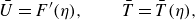 \begin{equation} {\bar {U}}=F^\prime (\eta ), \qquad {\bar {T}}={\bar {T}}(\eta ), \end{equation}
where $\eta$
is the similarity variable defined, via the Dorodnitsyn–Howarth coordinate transformation, by
$\eta$
is the similarity variable defined, via the Dorodnitsyn–Howarth coordinate transformation, by
 \begin{equation} \eta =\frac {1}{\sqrt {x_3}}\int _{0}^{y} \bar {R}\,\textrm {d} y. \end{equation}
In terms of $\eta$
,
$\eta$
, $F$
and
$F$
and $\bar {T}$
, the steady boundary-layer equations reduce to
$\bar {T}$
, the steady boundary-layer equations reduce to
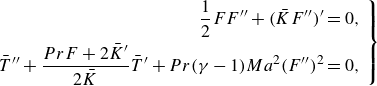 \begin{equation} \left .\begin{aligned} \frac {1}{2}FF^{\prime \prime }+(\bar {K} F^{\prime \prime })^\prime &=0, \\ {\bar {T}}^{\prime \prime }+\frac {PrF+2\bar {K}^\prime }{2\bar {K}}{\bar {T}}^\prime +Pr(\gamma -1)Ma^2(F^{\prime \prime })^2 &=0, \end{aligned}\,\,\right \} \end{equation}
where we have put $\bar {K}({\bar {T}})=\bar \mu ({\bar {T}})/{\bar {T}}$
. For Sutherland’s law,
$\bar {K}({\bar {T}})=\bar \mu ({\bar {T}})/{\bar {T}}$
. For Sutherland’s law, $\bar {K}$
is given by
$\bar {K}$
is given by
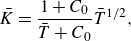 \begin{equation} \bar {K}=\frac {1+C_0}{{\bar {T}}+C_0}{\bar {T}}^{1/2}, \end{equation}
where $C_0=110.4\,{\textrm{K}}/T_\infty$
with
$C_0=110.4\,{\textrm{K}}/T_\infty$
with $T_\infty$
being the free stream temperature in Kelvin. The corresponding boundary conditions are
$T_\infty$
being the free stream temperature in Kelvin. The corresponding boundary conditions are
 \begin{equation} F(0)=F^\prime (0)=0; \qquad F^\prime \rightarrow 1 \quad \mbox{as}\quad \eta \rightarrow \infty , \end{equation}
and
 \begin{equation} {\bar {T}}(0)=\bar {T}_w; \qquad {\bar {T}}\rightarrow 1 \quad \mbox{as}\quad \eta \rightarrow \infty \end{equation}
if the wall is isothermal with a prescribed temperature $\bar {T}_w$
.
$\bar {T}_w$
.
We consider a perfect gas with ratio of specific heats $\gamma =1.4$
and Prandtl number
$\gamma =1.4$
and Prandtl number $Pr=0.72$
. The free stream temperature is taken to be
$Pr=0.72$
. The free stream temperature is taken to be $T_\infty =300\,{\textrm{K}}$
, and the Mach number
$T_\infty =300\,{\textrm{K}}$
, and the Mach number $Ma=6$
. The chosen parameters are representative of flight conditions (Chuvakhov & Fedorov Reference Chuvakhov and Fedorov2016). The base-flow equations (2.8) were solved using a shooting method based on a fourth-order Runge–Kutta integrator as in Qin & Wu (Reference Qin and Wu2024), where the streamwise velocity and temperature for various cooling ratios,
$Ma=6$
. The chosen parameters are representative of flight conditions (Chuvakhov & Fedorov Reference Chuvakhov and Fedorov2016). The base-flow equations (2.8) were solved using a shooting method based on a fourth-order Runge–Kutta integrator as in Qin & Wu (Reference Qin and Wu2024), where the streamwise velocity and temperature for various cooling ratios, $r_c$
, defined as the wall temperature over the adiabatic wall temperature, were presented.
$r_c$
, defined as the wall temperature over the adiabatic wall temperature, were presented.
The stability of the boundary layer is studied by introducing to it small-amplitude disturbances, $(\tilde \rho , \tilde {u}, \tilde {v}, \tilde {p}, \tilde \theta )$
, and the perturbed flow field can be written as
$(\tilde \rho , \tilde {u}, \tilde {v}, \tilde {p}, \tilde \theta )$
, and the perturbed flow field can be written as $(\rho , u, v, p, T)=(R_B, U_B, V_B, P_B, T_B)+(\tilde \rho , \tilde {u}, \tilde {v}, \tilde {p}, \tilde \theta )$
. For a neutral radiating mode, its pressure is governed by the Rayleigh equation, with the boundary condition consisting of the impermeability condition at the wall and a finite amplitude at infinity. Qin & Wu (Reference Qin and Wu2024) showed that a radiating mode exists only for
$(\rho , u, v, p, T)=(R_B, U_B, V_B, P_B, T_B)+(\tilde \rho , \tilde {u}, \tilde {v}, \tilde {p}, \tilde \theta )$
. For a neutral radiating mode, its pressure is governed by the Rayleigh equation, with the boundary condition consisting of the impermeability condition at the wall and a finite amplitude at infinity. Qin & Wu (Reference Qin and Wu2024) showed that a radiating mode exists only for $r_c$
below a certain value less than unity. In particular, using the base-flow quantities with
$r_c$
below a certain value less than unity. In particular, using the base-flow quantities with $r_c=0.427$
(
$r_c=0.427$
( $\bar {T}_w=3$
), a two-dimensional neutral radiating mode was found, whose streamwise wavenumber and phase velocity are
$\bar {T}_w=3$
), a two-dimensional neutral radiating mode was found, whose streamwise wavenumber and phase velocity are
 \begin{equation} \alpha =0.355336, \qquad c=0.723147. \end{equation}
This radiating mode and the particular base flow ( $r_c=0.427$
) will be used in our calculations. We choose to focus on a two-dimensional mode partly for simplicity and partly because its growth prior to becoming neutral is greater than that of the oblique modes. For adiabatic walls, a radiating mode does not exist at least for the present base-flow parameters. In this case, subsonic modes are important and likely influenced by impinging noise. However, the mechanism to be described in this paper does not apply to them, and one would have to seek viable alternative mechanisms for such modes.
$r_c=0.427$
) will be used in our calculations. We choose to focus on a two-dimensional mode partly for simplicity and partly because its growth prior to becoming neutral is greater than that of the oblique modes. For adiabatic walls, a radiating mode does not exist at least for the present base-flow parameters. In this case, subsonic modes are important and likely influenced by impinging noise. However, the mechanism to be described in this paper does not apply to them, and one would have to seek viable alternative mechanisms for such modes.
2.2. Free stream acoustic waves
Acoustic waves are an important type of elementary disturbances in the free stream. The density, velocity and pressure components of a two-dimensional acoustic wave, ${\epsilon _s}(\rho _s, u_s, v_s, p_s)$
, where
${\epsilon _s}(\rho _s, u_s, v_s, p_s)$
, where $\epsilon _s\ll 1$
is the magnitude, satisfy, to leading-order accuracy, the linearised Euler equations about the uniform background field. Eliminating
$\epsilon _s\ll 1$
is the magnitude, satisfy, to leading-order accuracy, the linearised Euler equations about the uniform background field. Eliminating $\rho _s$
,
$\rho _s$
, $u_s$
and
$u_s$
and $v_s$
from these equations leads to the equation for pressure
$v_s$
from these equations leads to the equation for pressure $p_s$
,
$p_s$
,
 \begin{equation} Ma^2\left ( \frac {\partial }{\partial {t}}+\frac {\partial }{\partial {x}} \right )^2 p_s-\nabla ^2 p_s=0. \end{equation}
The solution takes the form
 \begin{equation} p_s=p_I{\textrm{e}}^{\textrm{i}(\alpha _{s}{x}+\gamma _{s}{y}-\omega _{s}{t})}+\textrm{c.c.}, \end{equation}
where $\alpha _{s}$
and
$\alpha _{s}$
and $\gamma _{s}$
denote the streamwise and normal wavenumbers, respectively, and
$\gamma _{s}$
denote the streamwise and normal wavenumbers, respectively, and $\omega _{s}$
and
$\omega _{s}$
and $p_I$
denote the frequency and the rescaled intensity, respectively; here,
$p_I$
denote the frequency and the rescaled intensity, respectively; here, $\gamma _{s}$
is taken to be positive so that the group velocity in the wall-normal direction is negative, i.e. the disturbance represents an incoming wave. A two-dimensional sound wave is considered because only such a wave can, even with a small amplitude, influence the like neutral radiating mode through subharmonic resonance.
$\gamma _{s}$
is taken to be positive so that the group velocity in the wall-normal direction is negative, i.e. the disturbance represents an incoming wave. A two-dimensional sound wave is considered because only such a wave can, even with a small amplitude, influence the like neutral radiating mode through subharmonic resonance.
Substitution of (2.14) into (2.13) yields the dispersion relation for slow acoustic waves,
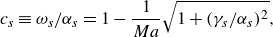 \begin{equation} c_s\equiv \omega _{s}/\alpha _{s}=1-\frac {1}{Ma}\sqrt {1+(\gamma _{s}/\alpha _{s})^2}, \end{equation}
where $c_s$
is the phase velocity. Here, as indicated by the sign of the second term on the right-hand-side, we have chosen to consider a slow sound wave, which has a critical layer, where the viscous effect has to be considered to obtain a regular solution and determine the reflection coefficient. The presence of this layer is instrumental for the sound wave to influence, even with a moderate amplitude, the radiating mode. In contrast, the fast sound wave has no critical layer, and is considered to be less effective in affecting the instability. We define an incident angle
$c_s$
is the phase velocity. Here, as indicated by the sign of the second term on the right-hand-side, we have chosen to consider a slow sound wave, which has a critical layer, where the viscous effect has to be considered to obtain a regular solution and determine the reflection coefficient. The presence of this layer is instrumental for the sound wave to influence, even with a moderate amplitude, the radiating mode. In contrast, the fast sound wave has no critical layer, and is considered to be less effective in affecting the instability. We define an incident angle $\theta _s$
by
$\theta _s$
by $\cos \theta _s=\alpha _{s}/\sqrt {\alpha _{s}^2+\gamma _{s}^2}$
. Use of (2.15) shows that
$\cos \theta _s=\alpha _{s}/\sqrt {\alpha _{s}^2+\gamma _{s}^2}$
. Use of (2.15) shows that
 \begin{equation} \theta _s=\cos ^{-1}\{1/[(1-c_s)Ma]\}. \end{equation}
A sound wave in the free stream is characterised by its frequency and incident angle. Since the slow acoustic wave that we consider is the first superharmonic of the radiating mode, the latter specifies its propagation direction.
2.3. Asymptotic scaling
We are interested in slow acoustic waves and instability modes with wavenumber $\alpha$
and frequency
$\alpha$
and frequency $\omega$
. Their wavelengths are comparable with the boundary-layer thickness (i.e.
$\omega$
. Their wavelengths are comparable with the boundary-layer thickness (i.e. $\alpha _{s}, \alpha =O(1)$
). When a slow acoustic wave impinges on the boundary layer, the response of the latter is in the form of an absorbed disturbance and a reflected wave. Subharmonic resonance takes place when the sound wave is the first superharmonic of the radiating mode, i.e.
$\alpha _{s}, \alpha =O(1)$
). When a slow acoustic wave impinges on the boundary layer, the response of the latter is in the form of an absorbed disturbance and a reflected wave. Subharmonic resonance takes place when the sound wave is the first superharmonic of the radiating mode, i.e.
 \begin{equation} \alpha _{s}=2\alpha , \qquad \omega _{s}=2\omega . \end{equation}
It follows from this relation that the oncoming sound wave shares a common critical level with the radiating mode, since
 \begin{equation} c_s=\omega _{s}/\alpha _{s}=\omega /\alpha =c. \end{equation}
The impinging acoustic wave affects the development of the instability mode through an effective quadratic interaction within the common critical layer. We will investigate this in the non-equilibrium parallel and equilibrium non-parallel regimes, respectively.
2.3.1. Non-equilibrium parallel regime
As an inviscid Rayleigh instability mode propagates downstream, its magnitude amplifies exponentially until it approaches the neutral position, $x_{3,n}$
say. Due to the accumulated growth, the mode is likely to enter a nonlinear stage in the vicinity of the neutral position (Goldstein & Leib Reference Goldstein and Leib1989; Wu 2019). Let this region be represented as
$x_{3,n}$
say. Due to the accumulated growth, the mode is likely to enter a nonlinear stage in the vicinity of the neutral position (Goldstein & Leib Reference Goldstein and Leib1989; Wu 2019). Let this region be represented as
 \begin{equation} x_3\approx x_{3,n}+\tilde \mu \bar {x}_1, \end{equation}
where $\tilde \mu \ll 1$
is to be determined in terms of
$\tilde \mu \ll 1$
is to be determined in terms of $\tilde \epsilon$
or
$\tilde \epsilon$
or $Re$
, and
$Re$
, and $\bar {x}_1=O(1)$
is negative. The local base-flow velocity and temperature profiles are expanded as
$\bar {x}_1=O(1)$
is negative. The local base-flow velocity and temperature profiles are expanded as
 \begin{equation} \Big ( {\bar {U}}(x_3, y), {\bar {T}}(x_3, y) \Big ) \approx \Big ( {\bar {U}}(x_{3,n}, y), {\bar {T}}(x_{3,n}, y) \Big ) +\tilde \mu \Big ( {\bar {U}}_1(y), {\bar {T}}_1(y) \Big )\bar {x}_1. \end{equation}
In this region, the growth rate of the mode is $O(\tilde \mu )$
, correspondingly, the amplitude develops over the length scale of
$O(\tilde \mu )$
, correspondingly, the amplitude develops over the length scale of $O(\tilde {\mu }^{-1})$
, and so we introduce the slow variable
$O(\tilde {\mu }^{-1})$
, and so we introduce the slow variable
 \begin{equation} \tilde {x}=\tilde \mu (x-x_0)=O(1) \quad \mbox{with}\quad x_0=Re(x_{3,n}+\tilde \mu \bar {x}_1). \end{equation}
The nonlinear evolution takes place in a region centred at $x_0$
with a length scale of
$x_0$
with a length scale of $O(\tilde {\mu }^{-1})$
, which is much larger than the boundary-layer thickness.
$O(\tilde {\mu }^{-1})$
, which is much larger than the boundary-layer thickness.
In the presence of the instability mode and an incident sound, the disturbance in the main layer can be expressed, to leading order, as
 \begin{align} (\tilde \rho , \tilde {u}, \tilde {v}, \tilde {p}, \tilde \theta )&=\tilde {\epsilon }A(\tilde {x}) \Big ( \hat {\rho }_0(y), \hat {u}_0(y), \hat {v}_0(y), \hat {p}_0(y), \hat {\theta }_0(y) \Big )E &+\tilde \epsilon _s(\check \rho _s, \check {u}_s, \check {v}_s, \check {p}_s, \check \theta _s)E_s\nonumber\\ &\quad +\textrm{c.c.}+\cdots , \end{align}
where $E={\textrm{e}}^{\textrm{i}\alpha \zeta }$
,
$E={\textrm{e}}^{\textrm{i}\alpha \zeta }$
, $\zeta =x-ct$
is the coordinate moving at the phase speed with
$\zeta =x-ct$
is the coordinate moving at the phase speed with $\alpha$
and
$\alpha$
and $c=\omega /\alpha$
being the streamwise wavenumber and phase speed, respectively, and
$c=\omega /\alpha$
being the streamwise wavenumber and phase speed, respectively, and $\tilde \epsilon \ll 1$
measures the magnitude of the radiating mode with
$\tilde \epsilon \ll 1$
measures the magnitude of the radiating mode with $A(\tilde {x})$
being the amplitude function describing its evolution; the second term in (2.22) represents the acoustic signature with
$A(\tilde {x})$
being the amplitude function describing its evolution; the second term in (2.22) represents the acoustic signature with $E_s={\textrm{e}}^{\textrm{i}\alpha _{s}(x-c_s t)}$
being its carrier wave, and
$E_s={\textrm{e}}^{\textrm{i}\alpha _{s}(x-c_s t)}$
being its carrier wave, and $\tilde \epsilon _s\ll 1$
measures the magnitude of the sound. The derivative with respect to
$\tilde \epsilon _s\ll 1$
measures the magnitude of the sound. The derivative with respect to $x$
then becomes
$x$
then becomes
 \begin{equation} \frac {\partial }{\partial {x}} \rightarrow \frac {\partial }{\partial \zeta }+\tilde \mu \frac {\partial }{\partial \tilde {x}}. \end{equation}
To derive the scaling, let us first write down the streamwise momentum equation (of the incompressible N-S equations for convenience) for the perturbation,
 \begin{equation} \bigg [ ({\bar {U}}-c)\frac {\partial }{\partial \zeta } +\tilde \mu {\bar {U}}\frac {\partial }{\partial \tilde {x}} \bigg ]\tilde {u}+\bar {U}^\prime \tilde {v} -Re^{-1}\frac {\partial ^2\tilde {u}}{\partial \tilde {y}^2}=-\frac {\partial \tilde {p}}{\partial \zeta } -\tilde {u}\frac {\partial \tilde {u}}{\partial \zeta }-\tilde {v}\frac {\partial \tilde {u}}{\partial y} -\tilde \mu \tilde {u}\frac {\partial \tilde {u}}{\partial \tilde {x}} +\cdots . \end{equation}
The scaling is fixed by considering the main and critical layers. In the main layer, the disturbance (the radiating mode and acoustic response included) remains, to the required order of accuracy, linear and inviscid, and the streamwise velocity of the radiating mode exhibits a jump of $O(\tilde {\epsilon }\tilde \mu )$
, which is to be determined by analysis of the critical layer (Goldstein & Leib Reference Goldstein and Leib1989). Suppose that the critical-layer width is
$O(\tilde {\epsilon }\tilde \mu )$
, which is to be determined by analysis of the critical layer (Goldstein & Leib Reference Goldstein and Leib1989). Suppose that the critical-layer width is $O(\delta _c)$
. It follows that the advection term in (2.24) is of
$O(\delta _c)$
. It follows that the advection term in (2.24) is of $O(\delta _c)$
, whereas the terms associated with the non-equilibrium and viscous effects are
$O(\delta _c)$
, whereas the terms associated with the non-equilibrium and viscous effects are $O(\tilde \mu )$
and
$O(\tilde \mu )$
and $O(Re^{-1}/\delta _c^2)$
, respectively. The requirement that these terms are all balanced leads to
$O(Re^{-1}/\delta _c^2)$
, respectively. The requirement that these terms are all balanced leads to
 \begin{equation} \delta _c=O\left(\tilde \mu \right), \qquad \delta _c=O\Big(Re^{-1/3}\Big). \end{equation}
In the critical layer, the wall-normal velocities of the radiating mode and acoustic response are of $O(\tilde {\epsilon })$
and
$O(\tilde {\epsilon })$
and $O(\tilde \epsilon _s)$
, respectively, but the logarithmic singularity
$O(\tilde \epsilon _s)$
, respectively, but the logarithmic singularity $\ln (y-y_c)$
of the inviscid solutions for the streamwise velocities suggests that the corresponding vorticities,
$\ln (y-y_c)$
of the inviscid solutions for the streamwise velocities suggests that the corresponding vorticities, $\tilde \epsilon \hat {u}_{0,y}$
and
$\tilde \epsilon \hat {u}_{0,y}$
and $\tilde \epsilon _s\check {u}_{s,y}$
, are of
$\tilde \epsilon _s\check {u}_{s,y}$
, are of $O(\tilde {\epsilon }\delta _c^{-1})$
and
$O(\tilde {\epsilon }\delta _c^{-1})$
and $O(\tilde \epsilon _s\delta _c^{-1})$
, respectively (Leib Reference Leib1991). Consideration of the self-nonlinear interactions of the radiating mode leading to the regeneration of the fundamental shows that if
$O(\tilde \epsilon _s\delta _c^{-1})$
, respectively (Leib Reference Leib1991). Consideration of the self-nonlinear interactions of the radiating mode leading to the regeneration of the fundamental shows that if $\tilde \mu =O(\tilde {\epsilon }^{2/5})$
, the nonlinear effect enters the amplitude equation (Leib Reference Leib1991; Wu & Cowley 1995). Under this scaling, the temperature fluctuation also contributes a nonlinear effect (Goldstein & Leib Reference Goldstein and Leib1989).
$\tilde \mu =O(\tilde {\epsilon }^{2/5})$
, the nonlinear effect enters the amplitude equation (Leib Reference Leib1991; Wu & Cowley 1995). Under this scaling, the temperature fluctuation also contributes a nonlinear effect (Goldstein & Leib Reference Goldstein and Leib1989).
However, in the common critical layer, the vorticity of the acoustic disturbance, $\tilde \epsilon _s\check {u}_{s,y}$
, is
$\tilde \epsilon _s\check {u}_{s,y}$
, is $O(\tilde \epsilon _s\delta _c^{-1})$
, as noted earlier. The forcing proportional to the product of the wall-normal velocity of the radiating mode
$O(\tilde \epsilon _s\delta _c^{-1})$
, as noted earlier. The forcing proportional to the product of the wall-normal velocity of the radiating mode $\tilde \epsilon \hat {v}_{0}$
and
$\tilde \epsilon \hat {v}_{0}$
and $\tilde \epsilon _s\check {u}_{s,y}$
is thus
$\tilde \epsilon _s\check {u}_{s,y}$
is thus $O(\tilde \epsilon \tilde \epsilon _s\delta _c^{-1})$
. Note that this forcing is of the form
$O(\tilde \epsilon \tilde \epsilon _s\delta _c^{-1})$
. Note that this forcing is of the form $E^*E_s=E$
according to (2.17), and represents the quadratic interaction of subharmonic resonance type between the radiating mode and the acoustic signature. It induces an
$E^*E_s=E$
according to (2.17), and represents the quadratic interaction of subharmonic resonance type between the radiating mode and the acoustic signature. It induces an $O(\tilde \epsilon \tilde \epsilon _s\delta _c^{-2})$
streamwise velocity of the fundamental as is deduced by balancing the forcing and the non-equilibrium terms in (2.24). This streamwise velocity exhibits a jump across the critical layer. If it is comparable with the
$O(\tilde \epsilon \tilde \epsilon _s\delta _c^{-2})$
streamwise velocity of the fundamental as is deduced by balancing the forcing and the non-equilibrium terms in (2.24). This streamwise velocity exhibits a jump across the critical layer. If it is comparable with the $O(\tilde {\epsilon }\tilde \mu )$
jump in the main layer, the subharmonic resonance effect enters the amplitude equation, leading to the characteristic threshold intensity of the sound
$O(\tilde {\epsilon }\tilde \mu )$
jump in the main layer, the subharmonic resonance effect enters the amplitude equation, leading to the characteristic threshold intensity of the sound
 \begin{equation} \tilde \epsilon _s=O\Big(\tilde \mu \delta _c^2\Big)=O\Big(\tilde \mu Re^{-2/3}\Big), \end{equation}
where use has been made of the second relation in (2.25).
With (2.25) and (2.26), we write
 \begin{equation} \tilde \mu =\tilde {\epsilon }^{2/5}=\delta _c, \qquad Re^{-1}=\lambda \tilde \mu ^3, \qquad \tilde \epsilon _s=\tilde {\epsilon }^{6/5}, \end{equation}
where $\lambda$
is the
$\lambda$
is the $O(1)$
Haberman parameter measuring the importance of viscosity. In terms of
$O(1)$
Haberman parameter measuring the importance of viscosity. In terms of $Re$
, the threshold sound intensity
$Re$
, the threshold sound intensity $\tilde \epsilon _s=O(Re^{-1})$
. The scaling relations (2.27) form the basis of non-equilibrium critical-layer theory describing the mutual interaction between the incident sound and the radiating mode as well as the self-interaction of the latter.
$\tilde \epsilon _s=O(Re^{-1})$
. The scaling relations (2.27) form the basis of non-equilibrium critical-layer theory describing the mutual interaction between the incident sound and the radiating mode as well as the self-interaction of the latter.
2.3.2. Equilibrium non-parallel regime
Non-parallelism is a salient feature of boundary-layer flows, and its effect on instability may be significant especially as a mode evolves through the vicinity of its neutral positions (Smith Reference Smith1979b ; Bodonyi & Smith Reference Bodonyi and Smith1981; Smith 1989). An asymptotic approach is required to characterise systematically the combined effects of non-parallelism and nonlinearity as shown by Smith (1979a) and Hall & Smith (Reference Hall and Smith1984) for lower-branch viscous T-S instability modes. For inviscid instability modes, such as the present radiating mode, the equilibrium non-parallel regime is pertinent to the region where the length scales over which the growth rate and the amplitude vary are comparable (Wu 2005). This region is represented by
 \begin{equation} x_3=x_{3,n}+Re^{-1/2}\bar {x} \quad \mbox{with}\quad \bar {x}=O(1). \end{equation}
We take $\delta ^*$
to be the boundary-layer thickness at the neutral position, and it follows that
$\delta ^*$
to be the boundary-layer thickness at the neutral position, and it follows that $x_{3,n}=1$
. Inspection of (2.24) shows that in this region, the non-equilibrium effect,
$x_{3,n}=1$
. Inspection of (2.24) shows that in this region, the non-equilibrium effect, $\bar \mu =O(Re^{-1/2})$
, is much smaller than the viscous effect. The critical layer is thus of equilibrium type and viscosity dominated, resulting in a critical layer width
$\bar \mu =O(Re^{-1/2})$
, is much smaller than the viscous effect. The critical layer is thus of equilibrium type and viscosity dominated, resulting in a critical layer width $\delta _c=O(Re^{-1/3})$
. A similar scaling argument shows that the self-nonlinear effect of the radiating mode comes into play when its amplitude reaches the threshold
$\delta _c=O(Re^{-1/3})$
. A similar scaling argument shows that the self-nonlinear effect of the radiating mode comes into play when its amplitude reaches the threshold
 \begin{equation} \tilde {\epsilon }=\delta _c^2\bar \mu ^{1/2}=O\Big(Re^{-11/12}\Big). \end{equation}
The quadratic interaction between the sound and the radiating mode regenerates the fundamental of the radiating mode with streamwise velocity of $O(\tilde \epsilon \tilde \epsilon _s\delta _c^{-2})$
. When this is comparable with the
$O(\tilde \epsilon \tilde \epsilon _s\delta _c^{-2})$
. When this is comparable with the $O(\tilde \epsilon Re^{-1/2})$
jump in the outer solution, i.e.
$O(\tilde \epsilon Re^{-1/2})$
jump in the outer solution, i.e. $\tilde \epsilon \tilde \epsilon _s\delta _c^{-2}=O(\tilde \epsilon Re^{-1/2})$
, the evolution of the radiating mode is affected by the incident sound wave. It follows that the threshold magnitude of the incident sound is
$\tilde \epsilon \tilde \epsilon _s\delta _c^{-2}=O(\tilde \epsilon Re^{-1/2})$
, the evolution of the radiating mode is affected by the incident sound wave. It follows that the threshold magnitude of the incident sound is
 \begin{equation} \tilde {\epsilon }_s=O\Big(Re^{-1/2}\delta _c^2\Big)=O\Big(Re^{-7/6}\Big), \end{equation}
which is asymptotically smaller than the $O(Re^{-1})$
threshold intensity in the non-equilibrium regime.
$O(Re^{-1})$
threshold intensity in the non-equilibrium regime.
The local mean velocity and temperature profiles can be approximated by
 \begin{equation} \Big ( {\bar {U}}(x_3, y), {\bar {T}}(x_3, y) \Big ) \approx \Big ( {\bar {U}}(x_{3,n}, y), {\bar {T}}(x_{3,n}, y) \Big ) +Re^{-1/2}\Big ( {\bar {U}}_1(y), {\bar {T}}_1(y) \Big )\bar {x}, \end{equation}
to the required order. With the key scalings identified, the effects of the sound wave on the evolution of the radiating mode will be analysed in a self-consistent manner.
The non-equilibrium parallel and equilibrium non-parallel regimes, while distinguished, are intrinsically linked. The connection can be understood by noting that (2.30), also follows from (2.26) by setting $\tilde \mu =O(Re^{-1/2})$
. The relation (2.26) holds in both regimes, and may be rewritten as
$\tilde \mu =O(Re^{-1/2})$
. The relation (2.26) holds in both regimes, and may be rewritten as
 \begin{equation} \tilde \mu =\tilde \epsilon _s Re^{2/3}, \end{equation}
which determines the growth-rate modification by the impinging sound in terms of its intensity. The modification is comparable to the local unmodified growth rate in the streamwise region specified by (2.19). The non-equilibrium parallel and equilibrium non-parallel regimes correspond to the distinguished thresholds $\tilde \epsilon _s=O(Re^{-1})$
and
$\tilde \epsilon _s=O(Re^{-1})$
and $O(Re^{-7/6})$
, respectively. As
$O(Re^{-7/6})$
, respectively. As $\tilde \epsilon _s$
is reduced from
$\tilde \epsilon _s$
is reduced from $O(Re^{-1})$
to
$O(Re^{-1})$
to $O(Re^{-7/6})$
, the non-equilibrium parallel regime acquires the character of the equilibrium non-parallel regime. This observation forms the basis for constructing the composite amplitude equation in § 4.
$O(Re^{-7/6})$
, the non-equilibrium parallel regime acquires the character of the equilibrium non-parallel regime. This observation forms the basis for constructing the composite amplitude equation in § 4.
The scaling relations derived earlier are pertinent to a two-dimensional radiating mode and an associated incident wave. We realise that a planar radiating mode can be continued to a band of oblique ones, each of which, $(\alpha , \beta , \omega )$
say, may be in resonance with an impinging sound wave
$(\alpha , \beta , \omega )$
say, may be in resonance with an impinging sound wave $(2\alpha , 2\beta , 2\omega )$
. Moreover, when a pair of oblique modes
$(2\alpha , 2\beta , 2\omega )$
. Moreover, when a pair of oblique modes $(\alpha , \pm \beta , \omega )$
are present, subharmonic triadic resonance (cf. Wu Reference Wu and Cowley1995) can take place between them and a planar sound wave
$(\alpha , \pm \beta , \omega )$
are present, subharmonic triadic resonance (cf. Wu Reference Wu and Cowley1995) can take place between them and a planar sound wave $(2\alpha , 0, 2\omega )$
. In these cases, the interactions are associated with the simple-pole singularity of the spanwise and streamwise velocities of the oblique mode(s), and the required threshold amplitude of the incident sound wave(s) would be
$(2\alpha , 0, 2\omega )$
. In these cases, the interactions are associated with the simple-pole singularity of the spanwise and streamwise velocities of the oblique mode(s), and the required threshold amplitude of the incident sound wave(s) would be $\tilde \epsilon _s=O(Re^{-4/3})$
and
$\tilde \epsilon _s=O(Re^{-4/3})$
and $O(Re^{-3/2})$
in the non-equilibrium parallel and equilibrium non-parallel regimes, respectively, as can be deduced by a similar scaling argument. These scenarios are interesting but are left for future investigation.
$O(Re^{-3/2})$
in the non-equilibrium parallel and equilibrium non-parallel regimes, respectively, as can be deduced by a similar scaling argument. These scenarios are interesting but are left for future investigation.
3. Subharmonic resonance
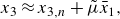
We consider the evolution of a pre-existing radiating mode in the presence of an impinging sound wave. The direct effect of the latter can be accounted for by an appropriate amplitude equation of the mode, which is to be derived. The physical process is illustrated in figure 1. The incident wave generates response within the boundary layer while being reflected. More importantly, it influences the development of the radiating mode through a subharmonic resonance and, in turn, the spontaneous emission of Mach waves. Depending on the intensity of the acoustic wave, the critical-layer dynamics takes two distinguished forms. The evolution of the radiating mode in both cases will be analysed in the following. Since much of the analysis is similar to that by Qin & Wu (Reference Qin and Wu2024), we outline, without repeating the derivations, the results in the earlier paper that are used in the present work, and our main focus will be on the new aspect: the interaction between the radiating mode and the acoustic signature.
A sketch of reflection of the sound wave and interaction with the radiating mode.
3.1. Non-equilibrium parallel regime
As the scaling relations in (2.27) indicate, the radiating mode evolves nonlinearly with the rate $\tilde \mu =\tilde {\epsilon }^{2/5}$
when its amplitude
$\tilde \mu =\tilde {\epsilon }^{2/5}$
when its amplitude $\tilde \epsilon =O(Re^{-5/6})$
, and is simultaneously affected by the incident sound with a smaller magnitude
$\tilde \epsilon =O(Re^{-5/6})$
, and is simultaneously affected by the incident sound with a smaller magnitude $\tilde {\epsilon }_s=\tilde {\epsilon }^{6/5}=O(Re^{-1})$
due to subharmonic resonance. Moreover, detuning effects may be included by allowing the wavenumber of the sound to differ from twice that of the radiating mode by an
$\tilde {\epsilon }_s=\tilde {\epsilon }^{6/5}=O(Re^{-1})$
due to subharmonic resonance. Moreover, detuning effects may be included by allowing the wavenumber of the sound to differ from twice that of the radiating mode by an $O(\tilde \mu )$
amount, that is,
$O(\tilde \mu )$
amount, that is,
 \begin{equation} \alpha _{s}=2\left(\alpha +\tilde \mu \tilde \alpha _d\right), \end{equation}
where $\tilde \alpha _d$
is an
$\tilde \alpha _d$
is an $O(1)$
detuning parameter.
$O(1)$
detuning parameter.
3.1.1. Main layer
In the main layer, the disturbance expands as
 \begin{align} \big(\tilde \rho , \tilde {u}, \tilde {v}, \tilde {p}, \tilde \theta \big)&= \tilde {\epsilon }\big [ \tilde {A}\big(\tilde {x}\big)\big(\hat {\rho }_0, \hat {u}_0, \hat {v}_0, \hat {p}_0, \hat {\theta }_0\big) +\tilde \mu \big(\hat {\rho }_1, \hat {u}_1, \hat {v}_1, \hat {p}_1, \hat {\theta }_1\big) \big ]E \\ &\quad \nonumber +\tilde \epsilon _s\big(\check \rho _s, \check {u}_s, \check {v}_s, \check {p}_s, \check \theta _s\big)E_s+\textrm{c.c.}+\cdots , \end{align}
where the first term represents a nearly neutral radiating mode, which propagates from upstream with $\tilde {A}(\tilde {x})$
being its amplitude function, and
$\tilde {A}(\tilde {x})$
being its amplitude function, and $E={\textrm{e}}^{\textrm{i}\alpha (x-ct)}$
its carrier wave. Here, the second term is the deviation from neutrality, while the third term represents the impinging acoustic perturbation with
$E={\textrm{e}}^{\textrm{i}\alpha (x-ct)}$
its carrier wave. Here, the second term is the deviation from neutrality, while the third term represents the impinging acoustic perturbation with $E_s={\textrm{e}}^{2\textrm{i}\alpha (x-ct)+2\textrm{i}\tilde {\alpha }_d\tilde {x}}$
being its carrier wave.
$E_s={\textrm{e}}^{2\textrm{i}\alpha (x-ct)+2\textrm{i}\tilde {\alpha }_d\tilde {x}}$
being its carrier wave.
Substitution of (3.2) into (2.2) followed by linearisation yields the leading-order equations for the mode,
 \begin{align} &\textrm{i}\alpha ({\bar {U}}-c)\hat {\rho }_0+\bar {R}^\prime \hat {v}_0+\bar {R}(\textrm{i}\alpha \hat {u}_0+\hat {v}_0^\prime )=0,\end{align}
 \begin{align} &\qquad\qquad\textrm{i}\alpha ({\bar {U}}-c)\hat {u}_0+{\bar {U}}^\prime \hat {v}_0=-\textrm{i}\alpha {\bar {T}}\hat {p}_0,\end{align}
 \begin{align} & \qquad\qquad \qquad\textrm{i}\alpha ({\bar {U}}-c)\hat {v}_0=-{\bar {T}}\hat {p}_0^\prime ,\end{align}
 \begin{align} &\textrm{i}\alpha ({\bar {U}}-c)\hat {\theta }_0+{\bar {T}}^\prime \hat {v}_0 =\textrm{i}\alpha (\gamma -1)Ma^2({\bar {U}}-c){\bar {T}}\hat {p}_0,\end{align}
 \begin{align} &\qquad\qquad\qquad\gamma Ma^2 \hat {p}_0=\bar {R}\hat {\theta }_0+{\bar {T}}\hat {\rho }_0.\end{align}
Elimination of $\hat {\rho }_0$
,
$\hat {\rho }_0$
, $\hat {u}_0$
,
$\hat {u}_0$
, $\hat {v}_0$
and
$\hat {v}_0$
and $\hat {\theta }_0$
leads to the compressible Rayleigh equation for
$\hat {\theta }_0$
leads to the compressible Rayleigh equation for $\hat {p}_0$
,
$\hat {p}_0$
,
 \begin{equation} \mathscr{L}\hat {p}_0\equiv \left \{ \frac {\partial ^2}{\partial y^2} +\left ( \frac {{\bar {T}}^\prime }{{\bar {T}}}-\frac {2{\bar {U}}^\prime }{{\bar {U}}-c} \right )\frac {\partial }{\partial y} -\alpha ^2\left [ 1-\frac {Ma^2({\bar {U}}-c)^2}{{\bar {T}}} \right ] \right \}\hat {p}_0=0. \end{equation}
As $y\rightarrow \infty$
,
$y\rightarrow \infty$
,
 \begin{equation} \hat {p}_0\sim \mathscr{C}_{\infty }{\textrm{e}}^{-\textrm{i}\alpha q y} \quad \mbox{with}\quad q=\sqrt {Ma^2(1-c)^2-1}, \end{equation}
which represents an outgoing wave that persists away from the main layer. Here, $\mathscr{C}_{\infty }$
is a constant that is determined by normalisation of the eigenfunction.
$\mathscr{C}_{\infty }$
is a constant that is determined by normalisation of the eigenfunction.
The solution near the critical level $y_c$
is obtained using the Frobenius method (Leib Reference Leib1991; Boyce & DiPrima Reference Boyce and DiPrima2012) as
$y_c$
is obtained using the Frobenius method (Leib Reference Leib1991; Boyce & DiPrima Reference Boyce and DiPrima2012) as
 \begin{equation} \hat {p}_0\sim \frac {\bar {U}_c^\prime }{\bar {T}_c}\bigg \{ \frac {\alpha ^2}{3}a^{\pm }\phi _a+\phi _b +\frac {\alpha ^2}{3}\bigg ( \frac {\bar {T}_c^\prime }{\bar {T}_c}-\frac {\bar {U}_c^{\prime \prime }}{\bar {U}_c^\prime } \bigg )\ln |{\hat {\eta }}|\phi _a \bigg \}, \end{equation}
where ${\hat {\eta }}\equiv y-y_c\rightarrow 0$
, and
${\hat {\eta }}\equiv y-y_c\rightarrow 0$
, and
 \begin{equation} \phi _{a}={\hat {\eta }}^3+\chi _{a}{\hat {\eta }}^4+\cdots , \qquad \phi _{b}=1-\frac {\alpha ^2}{2}{\hat {\eta }}^2+\chi _{b}{\hat {\eta }}^4+\cdots , \end{equation}
with $\chi _a$
and
$\chi _a$
and $\chi _b$
being constants, whose expressions are given by (3.8) and (3.9) of Qin & Wu (Reference Qin and Wu2024) with
$\chi _b$
being constants, whose expressions are given by (3.8) and (3.9) of Qin & Wu (Reference Qin and Wu2024) with $\alpha$
replacing
$\alpha$
replacing $\alpha _{s}$
, and are reproduced in Appendix A for completeness; here, the subscript
$\alpha _{s}$
, and are reproduced in Appendix A for completeness; here, the subscript $c$
represents the value evaluated at the critical level. It follows from (3.3b
)–(3.3d
) that as
$c$
represents the value evaluated at the critical level. It follows from (3.3b
)–(3.3d
) that as ${\hat {\eta }}\rightarrow 0$
,
${\hat {\eta }}\rightarrow 0$
,
 \begin{equation} \hat {u}_0\sim -\bigg ( \frac {\bar {T}_c^\prime }{\bar {T}_c}-\frac {\bar {U}_c^{\prime \prime }}{\bar {U}_c^\prime } \bigg )\ln |{\hat {\eta }}| +\frac {5}{6}\frac {\bar {U}_c^{\prime \prime }}{\bar {U}_c^\prime }-\frac {1}{3}\frac {\bar {T}_c^\prime }{\bar {T}_c}-a^{\pm }+\cdots , \end{equation}
 \begin{equation} \hat {v}_0\sim -\textrm{i}\alpha \bigg \{ 1-\bigg ( \frac {\bar {T}_c^\prime }{\bar {T}_c}-\frac {\bar {U}_c^{\prime \prime }}{\bar {U}_c^\prime } \bigg ){\hat {\eta }}\ln |{\hat {\eta }}| +\bigg ( \frac {2}{3}\frac {\bar {T}_c^\prime }{\bar {T}_c}-\frac {1}{6}\frac {\bar {U}_c^{\prime \prime }}{\bar {U}_c^\prime }-a^{\pm } \bigg ){\hat {\eta }} +\cdots \bigg \}, \end{equation}
 \begin{equation} \hat {\theta }_0\sim \frac {\bar {T}_c^\prime }{\bar {U}_c^\prime {\hat {\eta }}}. \end{equation}
The temperature perturbation exhibits the same simple-pole singularity as that of an inflectional mode (Goldstein & Leib Reference Goldstein and Leib1989), while the logarithmic singularity is present only for a supersonic mode, whose critical level does not correspond to the generalised inflection point (Leib Reference Leib1991). Equation (3.8) indicates a jump of $\hat {u}_0$
,
$\hat {u}_0$
,
 \begin{equation} \hat {u}_0^+ - \hat {u}_0^- = -(a^+ - a^-)+\cdots . \end{equation}
At the next order, the second terms in the expansion (3.2), $(\hat {\rho }_1, \hat {u}_1, \hat {v}_1, \hat {p}_1, \hat {\theta }_1)$
, are found to satisfy the inhomogeneous version of (3.3a
)–(3.3e
), which are given in Appendix A. By eliminating
$(\hat {\rho }_1, \hat {u}_1, \hat {v}_1, \hat {p}_1, \hat {\theta }_1)$
, are found to satisfy the inhomogeneous version of (3.3a
)–(3.3e
), which are given in Appendix A. By eliminating $\hat {\rho }_1$
,
$\hat {\rho }_1$
, $\hat {u}_1$
,
$\hat {u}_1$
, $\hat {v}_1$
and
$\hat {v}_1$
and $\hat {\theta }_1$
, we can show that
$\hat {\theta }_1$
, we can show that $\hat {p}_1$
satisfies an inhomogeneous Rayleigh equation (Wu 2005; Qin & Wu Reference Qin and Wu2024),
$\hat {p}_1$
satisfies an inhomogeneous Rayleigh equation (Wu 2005; Qin & Wu Reference Qin and Wu2024),
 \begin{equation} \mathscr{L}\hat {p}_1=\tilde {A}^\prime \frac {2\textrm{i} c}{\alpha }\bigg \{ \frac {\bar {U}^\prime \hat {p}_0^\prime }{({\bar {U}}-c)^2} +\frac {\alpha ^2}{c}\bigg [ \frac {Ma^2{\bar {U}}({\bar {U}}-c)}{{\bar {T}}}-1 \bigg ]\hat {p}_0 \bigg \} -\bar {x}_1 \tilde {A}\Delta _1, \end{equation}
where we have put
 \begin{equation} \varDelta _1\!=\!\bigg \{\! \frac {2\bar {U}^\prime }{{\bar {U}}-c}\bigg ( \frac {{\bar {U}}_1}{{\bar {U}}-c}-\frac {{\bar {U}}_1^\prime }{\bar {U}^\prime } \bigg ) +\frac {\bar {T}^\prime }{{\bar {T}}}\bigg ( \frac {{\bar {T}}_1^\prime }{\bar {T}^\prime }-\frac {{\bar {T}}_1}{{\bar {T}}} \bigg )\! \bigg \}\hat {p}_0^\prime +\alpha ^2 Ma^2\frac {({\bar {U}}-c)^2}{{\bar {T}}}\bigg ( \!\frac {2{\bar {U}}_1}{{\bar {U}}-c}-\frac {{\bar {T}}_1}{{\bar {T}}}\! \bigg )\hat {p}_0. \end{equation}
As $y\rightarrow \infty$
,
$y\rightarrow \infty$
,
 \begin{equation} \hat {p}_1\sim p_R(\tilde {x}){\textrm{e}}^{-\textrm{i}\alpha q y} +q^{-1}[1-Ma^2(1-c)]\mathscr{C}_{\infty }\tilde {A}^\prime y{\textrm{e}}^{-\textrm{i}\alpha q y}. \end{equation}
However, by the method of dominant balance, we deduce that as $y\rightarrow y_c$
,
$y\rightarrow y_c$
,
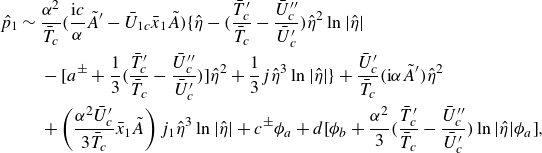 \begin{align} \hat {p}_1 &\sim \frac {\alpha ^2}{\bar {T}_c}\bigg ( \frac {\textrm{i} c}{\alpha }\tilde {A}^\prime -{\bar {U}}_{1c}\bar {x}_1 \tilde {A} \bigg ) \bigg \{ {\hat {\eta }}-\bigg ( \frac {\bar {T}_c^\prime }{\bar {T}_c}-\frac {\bar {U}_c^{\prime \prime }}{\bar {U}_c^\prime } \bigg ){\hat {\eta }}^2\ln |{\hat {\eta }}| \\ \nonumber &\quad \, -\bigg [ a^{\pm }+\frac {1}{3}\bigg ( \frac {\bar {T}_c^\prime }{\bar {T}_c}-\frac {\bar {U}_c^{\prime \prime }}{\bar {U}_c^\prime } \bigg ) \bigg ]{\hat {\eta }}^2 +\frac {1}{3}j{\hat {\eta }}^3\ln |{\hat {\eta }}| \bigg \}+\frac {\bar {U}_c^\prime }{\bar {T}_c}(\textrm{i}\alpha \tilde {A}^\prime ){\hat {\eta }}^2 \\ \nonumber &\quad \, +\left ( \frac {\alpha ^2\bar {U}_c^\prime }{3\bar {T}_c}\bar {x}_1 \tilde {A} \right )j_1{\hat {\eta }}^3\ln |{\hat {\eta }}| +c^{\pm }\phi _a +d\bigg [ \phi _b+\frac {\alpha ^2}{3}\bigg ( \frac {\bar {T}_c^\prime }{\bar {T}_c}-\frac {\bar {U}_c^{\prime \prime }}{\bar {U}_c^\prime } \bigg )\ln |{\hat {\eta }}|\phi _a \bigg ], \end{align}
where $c^{\pm }$
and
$c^{\pm }$
and $d$
are arbitrary functions of
$d$
are arbitrary functions of $\tilde {x}$
, and
$\tilde {x}$
, and
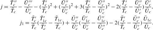 \begin{align} j=\frac {\bar {T}_c^{\prime \prime }}{\bar {T}_c}-\frac {\bar {U}_c^{\prime \prime \prime }}{\bar {U}_c^\prime } -\bigg ( \frac {\bar {T}_c^\prime }{\bar {T}_c} \bigg )^2 +\bigg ( \frac {\bar {U}_c^{\prime \prime }}{\bar {U}_c^\prime } \bigg )^2 +3\bigg ( \frac {\bar {T}_c^\prime }{\bar {T}_c}-\frac {\bar {U}_c^{\prime \prime }}{\bar {U}_c^\prime } \bigg )^2 -2\bigg ( \frac {\bar {T}_c^\prime }{\bar {T}_c}-\frac {\bar {U}_c^{\prime \prime }}{\bar {U}_c^\prime } \bigg )\frac {\bar {U}_c^\prime }{\bar {U}_c},\nonumber \\ j_1=\frac {\bar {T}_c^\prime }{\bar {T}_c}\bigg ( \frac {{\bar {T}}_{1c}^\prime }{\bar {T}_c^\prime }-\frac {{\bar {T}}_{1c}}{\bar {T}_c} \bigg ) +\frac {\bar {U}_c^{\prime \prime }}{\bar {U}_c^\prime }\bigg ( \frac {{\bar {U}}_{1c}^\prime }{\bar {U}_c^\prime }-\frac {{\bar {U}}_{1c}^{\prime \prime }}{\bar {U}_c^{\prime \prime }} \bigg ) -2\bigg ( \frac {\bar {T}_c^\prime }{\bar {T}_c}-\frac {\bar {U}_c^{\prime \prime }}{\bar {U}_c^\prime } \bigg )\frac {{\bar {U}}_{1c}}{\bar {U}_c}. \end{align}
It follows from the $x$
- and
$x$
- and $y$
-momentum equations, (A3b) and (A3c
), that
$y$
-momentum equations, (A3b) and (A3c
), that
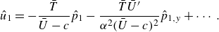 \begin{equation} \hat {u}_1=-\frac {{\bar {T}}}{{\bar {U}}-c}\hat {p}_1-\frac {{\bar {T}}\bar {U}^\prime }{\alpha ^2({\bar {U}}-c)^2}\hat {p}_{1,y}+\cdots . \end{equation}
Thus, the jump of $\hat {u}_1$
is found to relate to
$\hat {u}_1$
is found to relate to $(c^+ - c^-)$
by the equation
$(c^+ - c^-)$
by the equation
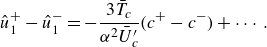 \begin{equation} \hat {u}_1^+ - \hat {u}_1^- = -\frac {3\bar {T}_c}{\alpha ^2\bar {U}_c^\prime }(c^+ - c^-)+\cdots . \end{equation}
For the inhomogeneous equation (3.12) to have an acceptable solution, it has to satisfy a solvability condition. This can be derived by multiplying both sides of (3.12) by $\hat {p}_0{\bar {T}}/({\bar {U}}-c)^2$
and integrating from
$\hat {p}_0{\bar {T}}/({\bar {U}}-c)^2$
and integrating from $0$
to
$0$
to $\infty$
, leading to
$\infty$
, leading to
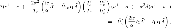 \begin{align} 3(c^{+}-c^{-})-\frac {2\alpha ^2}{\bar {T}_c} \left ( \frac {\textrm{i} c}{\alpha }\tilde {A}^\prime -{\bar {U}}_{1c}\bar {x}_1 \tilde {A} \right ) \left ( \frac {\bar {T}_c^\prime }{\bar {T}_c}-\frac {\bar {U}_c^{\prime \prime }}{\bar {U}_c^\prime } \right )(a^{+}-a^{-}) -\alpha ^2 d(a^{+}-a^{-})\nonumber \\ =-\bar {U}_c^\prime \left (\frac {2\textrm{i} c}{\alpha }I_2 \tilde {A}^\prime -I_1\bar {x}_1 \tilde {A}\right ), \end{align}
where use has been made of the impermeability condition $\hat {p}_0^\prime (0)=\hat {p}_{1,y}|_{y=0}=0$
and the far-field condition (3.5) and (3.14), and the expressions for the integrals,
$\hat {p}_0^\prime (0)=\hat {p}_{1,y}|_{y=0}=0$
and the far-field condition (3.5) and (3.14), and the expressions for the integrals, $I_1$
and
$I_1$
and $I_2$
, are given by (4.19) and (4.20) of Qin & Wu (Reference Qin and Wu2024), respectively, and are reproduced in Appendix A for completeness. The jumps
$I_2$
, are given by (4.19) and (4.20) of Qin & Wu (Reference Qin and Wu2024), respectively, and are reproduced in Appendix A for completeness. The jumps $(a^{+}-a^{-})$
and
$(a^{+}-a^{-})$
and $(c^{+}-c^{-})$
will be determined by analysing the critical-layer dynamics.
$(c^{+}-c^{-})$
will be determined by analysing the critical-layer dynamics.
The acoustic components, $(\check \rho _s, \check {u}_s, \check {v}_s, \check {p}_s, \check \theta _s)$
, satisfy the same equation as (3.3) with
$(\check \rho _s, \check {u}_s, \check {v}_s, \check {p}_s, \check \theta _s)$
, satisfy the same equation as (3.3) with $\alpha _{s}$
and
$\alpha _{s}$
and $c_s$
replacing
$c_s$
replacing $\alpha$
and
$\alpha$
and $c$
, respectively. Elimination of
$c$
, respectively. Elimination of $\check \rho _s$
,
$\check \rho _s$
, $\check {u}_s$
,
$\check {u}_s$
, $\check {v}_s$
and
$\check {v}_s$
and $\check \theta _s$
leads to the familiar compressible Rayleigh equation for pressure
$\check \theta _s$
leads to the familiar compressible Rayleigh equation for pressure $\check {p}_s$
,
$\check {p}_s$
, $\mathscr{L}{\check {p}_s}=0$
. This equation must be solved subject to the impermeability condition,
$\mathscr{L}{\check {p}_s}=0$
. This equation must be solved subject to the impermeability condition, $\check {p}_{s,y}(0)=0$
. In the far field, the pressure takes the form
$\check {p}_{s,y}(0)=0$
. In the far field, the pressure takes the form
 \begin{equation} \check {p}_s\sim p_I\left[{\textrm{e}}^{\textrm{i}\gamma _{s} y}+\mathscr{R}\,{\textrm{e}}^{-\textrm{i}\gamma _{s} y}\right] \quad \mbox{as}\quad y\rightarrow \infty , \end{equation}
which consists of an incident wave and a reflected wave, where $\gamma _{s}=\alpha _{s}\sqrt {Ma^2(1-c_s)^2-1}$
, and
$\gamma _{s}=\alpha _{s}\sqrt {Ma^2(1-c_s)^2-1}$
, and $\mathscr{R}$
is the reflection coefficient. As
$\mathscr{R}$
is the reflection coefficient. As ${\hat {\eta }}\rightarrow 0$
, the local solution to
${\hat {\eta }}\rightarrow 0$
, the local solution to $\mathscr{L}{\check {p}_s}=0$
is constructed by using the Frobenius method as
$\mathscr{L}{\check {p}_s}=0$
is constructed by using the Frobenius method as
 \begin{equation} \check {p}_s=a_s^\pm \phi _{sa}+b_s^\pm \left [ \phi _{sb} +\frac {\alpha _{s}^2}{3}\left ( \frac {\bar {T}_c^\prime }{\bar {T}_c}-\frac {\bar {U}_c^{\prime \prime }}{\bar {U}_c^\prime } \right )\ln |{\hat {\eta }}|\phi _{sa} \right ], \end{equation}
where $\phi _{sa}$
and
$\phi _{sa}$
and $\phi _{sb}$
have the same expressions as
$\phi _{sb}$
have the same expressions as $\phi _a$
and
$\phi _a$
and $\phi _b$
given by (3.7), with
$\phi _b$
given by (3.7), with $\alpha _{s}$
replacing
$\alpha _{s}$
replacing $\alpha$
. The pressure, velocities and temperature of the acoustic disturbance have the expressions
$\alpha$
. The pressure, velocities and temperature of the acoustic disturbance have the expressions
 \begin{equation} \check {p}_s=b_s^\pm \left [ 1-\frac {\alpha _{s}^2}{2}{\hat {\eta }}^2+\frac {\alpha _{s}^2}{3} \left ( \frac {\bar {T}_c^\prime }{\bar {T}_c}-\frac {\bar {U}_c^{\prime \prime }}{\bar {U}_c^\prime } \right ){\hat {\eta }}^3\ln |{\hat {\eta }}| +(a_s^\pm /b_s^\pm ){\hat {\eta }}^3 \right ]+O({\hat {\eta }}^4\ln |{\hat {\eta }}|), \end{equation}
 \begin{equation} \check {v}_s=-\textrm{i}\alpha _{s} b_s^\pm \frac {\bar {T}_c}{\bar {U}_c^\prime }\left [ \!1- \left ( \frac {\bar {T}_c^\prime }{\bar {T}_c}-\frac {\bar {U}_c^{\prime \prime }}{\bar {U}_c^\prime } \right ){\hat {\eta }}\ln |{\hat {\eta }}| +\left ( \frac {2}{3}\frac {\bar {T}_c^\prime }{\bar {T}_c}-\frac {1}{6}\frac {\bar {U}_c^{\prime \prime }}{\bar {U}_c^\prime } -\frac {3a_s^\pm }{\alpha _{s}^2 b_s^\pm } \right ){\hat {\eta }}\! \right ]\!+\!O({\hat {\eta }}^2\ln |{\hat {\eta }}|), \end{equation}
 \begin{equation} \check {u}_s=b_s^\pm \frac {\bar {T}_c}{\bar {U}_c^\prime }\left [ -\left ( \frac {\bar {T}_c^\prime }{\bar {T}_c}-\frac {\bar {U}_c^{\prime \prime }}{\bar {U}_c^\prime } \right )\ln |{\hat {\eta }}| +\frac {5}{6}\frac {\bar {U}_c^{\prime \prime }}{\bar {U}_c^\prime }-\frac {1}{3}\frac {\bar {T}_c^\prime }{\bar {T}_c} -\frac {3a_s^\pm }{\alpha _{s}^2 b_s^\pm } \right ]+O({\hat {\eta }}\ln |{\hat {\eta }}|), \end{equation}
 \begin{equation} \check \theta _s=b_s^\pm \frac {\bar {T}_c\bar {T}_c^\prime }{(\bar {U}_c^\prime )^2}\left [ \frac {1}{{\hat {\eta }}} -\left ( \frac {\bar {T}_c^\prime }{\bar {T}_c}-\frac {\bar {U}_c^{\prime \prime }}{\bar {U}_c^\prime } \right )\ln |{\hat {\eta }}| \right ]+O(1). \end{equation}
It is worth noting that in the main layer and free stream, the acoustic wave and radiating mode bear much resemblance, both being governed by linearised Euler equations and having similar forms of solutions. Clearly, the temperature perturbation $\check \theta _s$
and the streamwise velocity
$\check \theta _s$
and the streamwise velocity $\check {u}_s$
exhibit a simple-pole singularity and a logarithmic singularity, respectively, indicating that the main-layer solution breaks down as
$\check {u}_s$
exhibit a simple-pole singularity and a logarithmic singularity, respectively, indicating that the main-layer solution breaks down as ${\hat {\eta }}\rightarrow 0$
. Thus we need to analyse the critical layer.
${\hat {\eta }}\rightarrow 0$
. Thus we need to analyse the critical layer.
3.1.2. Critical layer
The singularity of the main-layer solution is to be removed by introducing viscous effects within the critical layer, which determine the critical layer width to be of order $Re^{-1/3}$
, which is
$Re^{-1/3}$
, which is $O(\tilde {\epsilon }^{2/5})$
, and so the appropriate local transverse coordinate is
$O(\tilde {\epsilon }^{2/5})$
, and so the appropriate local transverse coordinate is
 \begin{equation} Y=(y-y_c)/\tilde {\epsilon }^{2/5}. \end{equation}
The asymptote of the inviscid solution, (3.6) and (3.8)–(3.10), suggests that the perturbation in the critical layer expands as
 \begin{align} \tilde {u}=\tilde {\epsilon }\Big(U_{1}E+\tilde {\epsilon }^{1/5}U_{M}+\tilde {\epsilon }^{2/5}U_{2}E\Big) +\tilde \epsilon _s U_{s1}E_s+\textrm{c.c.}+\cdots , \\[-12pt] \nonumber \end{align}
 \begin{align} \tilde {v}=\tilde {\epsilon }\Big(V_{0}E+\tilde {\epsilon }^{2/5}V_{1}E+\tilde {\epsilon }^{3/5}V_{M} +\tilde {\epsilon }^{4/5}V_{2}E\Big)+\tilde \epsilon _s V_{s0}E_s+\textrm{c.c.}+\cdots , \\[-12pt] \nonumber \end{align}
 \begin{align} \tilde {p}=\tilde {\epsilon }\Big(P_{0}E+\tilde {\epsilon }^{2/5}P_{1}E+\tilde {\epsilon }^{4/5}P_{2}E\Big) +\tilde \epsilon _s P_{s0}E_s+\textrm{c.c.}+\cdots , \\[-12pt] \nonumber \end{align}
 \begin{align} \tilde \theta =\tilde {\epsilon }^{3/5}\Big(\Theta _{1}E+\tilde {\epsilon }^{1/5}\Theta _{M} +\tilde {\epsilon }^{2/5}\Theta _{2}E\Big)+\tilde \epsilon _s\tilde {\epsilon }^{-2/5}\Theta _{s1}E_s+\textrm{c.c.}+\cdots ,\end{align}
where the subscript $M$
denotes the mean-flow distortion. Strictly speaking, the expansions actually contain logarithm terms, but they are not needed in the calculation of the jumps and hence are not written out for brevity. Substituting (3.24) into (2.2) and noting (2.23) and (3.23), we then obtain the equations governing the terms at different orders in the expansion.
$M$
denotes the mean-flow distortion. Strictly speaking, the expansions actually contain logarithm terms, but they are not needed in the calculation of the jumps and hence are not written out for brevity. Substituting (3.24) into (2.2) and noting (2.23) and (3.23), we then obtain the equations governing the terms at different orders in the expansion.
At leading order, inspection of the $x$
- and
$x$
- and $y$
-momentum equations gives
$y$
-momentum equations gives
 \begin{equation} P_0=\Big(\bar {U}_c^\prime /\bar {T}_c\Big)\tilde {A}, \qquad V_0=-\textrm{i}\alpha \tilde {A}. \end{equation}
Expansion of the energy equation shows that
 \begin{equation} \mathscr{L}_p\Theta _{1}+{\bar {T}_c^\prime }V_{0}=0, \end{equation}
with the operator $\mathscr{L}_p$
being defined by
$\mathscr{L}_p$
being defined by
 \begin{equation} \mathscr{L}_p=c\frac {\partial }{\partial \tilde {x}}+ \textrm{i}\alpha \Big(\bar {U}_c^\prime Y+{\bar {U}}_{1c}\bar {x}_1\Big)-\lambda \bar {T}_c\bar {\mu }_c Pr^{-1}\frac {\partial ^2}{\partial Y^2}. \end{equation}
Equation (3.26) is solved by use of Fourier transform to give
 \begin{equation} \Theta _1=\textrm{i}\alpha \bar {T}_c^\prime \int _{0}^{\infty } \exp \Big(-s_p\xi ^3-\textrm{i}\alpha \bar {U}_c^\prime \bar {Y}\xi \Big)\tilde {A}(\tilde {x}-c\xi )\,\textrm {d}\xi , \end{equation}
where we have put $\bar {Y}\equiv Y+({\bar {U}}_{1c}/\bar {U}_c^\prime )\bar {x}_1$
and
$\bar {Y}\equiv Y+({\bar {U}}_{1c}/\bar {U}_c^\prime )\bar {x}_1$
and $s_p={\textstyle {1}/{3}}\lambda (\alpha \bar {U}_c^\prime )^2\bar {T}_c\bar {\mu }_c Pr^{-1}$
.
$s_p={\textstyle {1}/{3}}\lambda (\alpha \bar {U}_c^\prime )^2\bar {T}_c\bar {\mu }_c Pr^{-1}$
.
At the next order, expansion of the continuity and $x$
-momentum equations yields
$x$
-momentum equations yields
 \begin{align} & -c\Theta _{1,\tilde {x}}/\bar {T}_c^2+\textrm{i}\alpha \Big(\bar {U}_c^\prime Y+{\bar {U}}_{1c}\bar {x}_1\Big)\Big(-\Theta _{1}/\bar {T}_c^2\Big) +\frac {1}{\bar {T}_c}\left(\textrm{i}\alpha U_1+V_{1,Y}\right)-\frac {\bar {T}_c^\prime }{\bar {T}_c^2}V_{0}=0,\end{align}
 \begin{align}& \mathscr{L}_\mu U_{1}+{\bar {U}_c^\prime }V_{1}+\left({\bar {U}_c^{\prime \prime }}Y+{\bar {U}}_{1c}^\prime \bar {x}_1\right)V_{0} =-\textrm{i}\alpha \bar {T}_c P_1-\bar {T}_c P_{0,\tilde {x}}-\textrm{i}\alpha \left(\bar {T}_c^\prime Y+{\bar {T}}_{1c}\bar {x}_1\right)P_0\nonumber \\ &\qquad\qquad\qquad +\lambda \bar {T}_c\bar {\mu }_c^\prime \bar {U}_c^\prime \Theta _{1,Y},\end{align}
where $\bar {\mu }_c^\prime =(\textrm {d}\bar \mu /\textrm {d}{\bar {T}})|_{y=y_c}$
, and
$\bar {\mu }_c^\prime =(\textrm {d}\bar \mu /\textrm {d}{\bar {T}})|_{y=y_c}$
, and $\mathscr{L}_\mu$
is the same as
$\mathscr{L}_\mu$
is the same as $\mathscr{L}_p$
provided that
$\mathscr{L}_p$
provided that $Pr$
is set to unity; here, the subscript
$Pr$
is set to unity; here, the subscript $Y$
denotes the differentiation with respect to
$Y$
denotes the differentiation with respect to $Y$
. These two equations are combined to obtain an equation for
$Y$
. These two equations are combined to obtain an equation for $U_{1,Y}$
, which is solved to give
$U_{1,Y}$
, which is solved to give
 \begin{align} U_{1,Y}\!=\!\textrm{i}\alpha \bar {U}_c^\prime \frac {\bar {T}_c^\prime \left(\bar {T}_c\bar {\mu }_c^\prime\! -\!\bar {\mu }_c Pr^{-1}\right)}{\bar {T}_c\bar {\mu }_c(1\!-\!Pr^{-1})} \!\!\int _{0}^{\infty } \left[ \!1\!-\!{\textrm{e}}^{-(s_p-s)\xi ^3} \right ] \exp \Big(\!-s\xi ^3-\textrm{i}\alpha \bar {U}_c^\prime \bar {Y}\xi \Big)\tilde {A}\!\left(\tilde {x}-c\xi \right)\textrm {d}\xi\nonumber \\ -\textrm{i}\alpha \bar {U}_c^\prime \bigg ( \frac {\bar {T}_c^\prime }{\bar {T}_c}-\frac {\bar {U}_c^{\prime \prime }}{\bar {U}_c^\prime } \bigg ) \!\!\int _{0}^{\infty } \exp \Big(-s\xi ^3-\textrm{i}\alpha \bar {U}_c^\prime \bar {Y}\xi \Big)\tilde {A}\left(\tilde {x}-c\xi \right)\textrm {d}\xi , \end{align}
where $s={\textstyle {1}/{3}}\lambda (\alpha \bar {U}_c^\prime )^2\bar {T}_c\bar {\mu }_c$
. Matching
$s={\textstyle {1}/{3}}\lambda (\alpha \bar {U}_c^\prime )^2\bar {T}_c\bar {\mu }_c$
. Matching $U_1$
with its outer counterpart determines the jump
$U_1$
with its outer counterpart determines the jump
 \begin{equation} a^+ - a^- = \bigg ( \frac {\bar {T}_c^\prime }{\bar {T}_c}-\frac {\bar {U}_c^{\prime \prime }}{\bar {U}_c^\prime } \bigg )\pi \textrm{i}. \end{equation}
We now consider the acoustic component. At leading order, the $y$
-momentum equation gives
$y$
-momentum equation gives $P_{s0,Y}=0$
. Matching with the main-layer solution leads to
$P_{s0,Y}=0$
. Matching with the main-layer solution leads to
 \begin{equation} b_s^+=P_{s0}=b_s^-\equiv b_s. \end{equation}
The continuity, $x$
-momentum and energy equations for the leading-order terms read
$x$
-momentum and energy equations for the leading-order terms read $V_{s0,Y}=0$
, and
$V_{s0,Y}=0$
, and
 \begin{align} \bar {U}_c^\prime V_{s0}&=-\textrm{i}\alpha _{s}\bar {T}_c P_{s0},\end{align}
 \begin{align} \textrm{i}\alpha _{s}\bar {U}_c^\prime Y \Theta _{s0}+\bar {T}_c^\prime V_{s0}&=\lambda \bar {T}_c\bar {\mu }_c Pr^{-1}\Theta _{s0,YY},\end{align}
respectively. The solution is found to be
 \begin{align} & \qquad\qquad\qquad\qquad\qquad V_{s0}=-\textrm{i}\alpha _{s} b_s\bar {T}_c/\bar {U}_c^\prime ,\end{align}
 \begin{align} \Theta _{s0}&=\textrm{i}\alpha _{s}\frac {\bar {T}_c\bar {T}_c^\prime }{\bar {U}_c^\prime }b_s \int _{0}^{\infty } \exp \Big(-s_{sp}\xi ^3-\textrm{i}\alpha _{s}\bar {U}_c^\prime Y\xi \Big)\textrm {d}\xi \, \mbox{with}\quad s_{sp}={\textstyle \frac {1}{3}}\lambda \left(\alpha _{s}\bar {U}_c^\prime \right)^2\bar {T}_c\bar {\mu }_c Pr^{-1}.\end{align}
At the next order, the continuity and $x$
-momentum equations yield
$x$
-momentum equations yield
 \begin{align} \textrm{i}\alpha _{s}\bar {U}_c^\prime Y(-\Theta _{s0}/\bar {T}_c^2)+(\textrm{i}\alpha _{s} U_{s1}+V_{s1,Y})/\bar {T}_c -(\bar {T}_c^\prime /\bar {T}_c^2)V_{s0}=0, \\[-10pt] \nonumber \end{align}
 \begin{align} \mathscr{L}_s U_{s1}+\bar {U}_c^\prime V_{s1}+\bar {U}_c^{\prime \prime } Y V_{s0} =-\textrm{i}\alpha _{s}\bar {T}_c^\prime Y P_{s0}+\lambda \bar {T}_c\bar {U}_c^\prime \bar {\mu }_c^\prime \Theta _{s0,Y},\end{align}
where the operator $\mathscr{L}_s$
is defined by
$\mathscr{L}_s$
is defined by
 \begin{equation} \mathscr{L}_s=\textrm{i}\alpha _{s}\bar {U}_c^\prime Y-\lambda \bar {T}_c\bar {\mu }_c\frac {\partial ^2}{\partial Y^2}. \end{equation}
Eliminating $V_{s1}$
between (3.35a
) and (3.35b
), and solving the resulting equation, we obtain
$V_{s1}$
between (3.35a
) and (3.35b
), and solving the resulting equation, we obtain
 \begin{align} U_{s1,Y}=\textrm{i}\alpha _{s}\frac {\bar {T}_c^\prime (\bar {T}_c\bar {\mu }_c^\prime -\bar {\mu }_c Pr^{-1})}{\bar {\mu }_c(1-Pr^{-1})}b_s \!\!\int _{0}^{\infty }\! \Big [ 1\!-\!\exp (-(s_{sp}-s_s)\xi ^3) \Big ]\exp (-s_s\xi ^3\!-\!\textrm{i}\alpha _{s}\bar {U}_c^\prime Y\xi )\,\textrm {d}\xi\nonumber \\ -\textrm{i}\alpha _{s}\bar {T}_c\bigg ( \frac {\bar {T}_c^\prime }{\bar {T}_c}-\frac {\bar {U}_c^{\prime \prime }}{\bar {U}_c^\prime } \bigg )b_s \int _{0}^{\infty } \exp (-s_s\xi ^3-\textrm{i}\alpha _{s}\bar {U}_c^\prime Y\xi )\,\textrm {d}\xi , \end{align}
where $s_s={\textstyle {1}/{3}}\lambda (\alpha _{s}\bar {U}_c^\prime )^2\bar {T}_c\bar {\mu }_c$
. Matching
$s_s={\textstyle {1}/{3}}\lambda (\alpha _{s}\bar {U}_c^\prime )^2\bar {T}_c\bar {\mu }_c$
. Matching $U_{s1}$
with its outer counterpart (3.22c
) determines the jump
$U_{s1}$
with its outer counterpart (3.22c
) determines the jump
 \begin{equation} a_s^+ - a_s^- = \frac {\alpha _{s}^2}{3} \bigg ( \frac {\bar {T}_c^\prime }{\bar {T}_c}-\frac {\bar {U}_c^{\prime \prime }}{\bar {U}_c^\prime } \bigg )b_s\pi \textrm{i}. \end{equation}
This jump is used together with (3.21) to solve the Rayleigh equation numerically where by we obtain the reflection coefficient $\mathscr{R}$
and the boundary-layer response
$\mathscr{R}$
and the boundary-layer response $b_s$
; the details were given by Qin & Wu (Reference Qin and Wu2024). There it was showed that both
$b_s$
; the details were given by Qin & Wu (Reference Qin and Wu2024). There it was showed that both $\mathscr{R}$
and
$\mathscr{R}$
and $b_s$
are extraordinarily large for a small subset of the sound incident angle and frequency. Furthermore, resonant over-reflection occurs for a specific pairing of incidence angle and frequency, and the reflected wave coincides with a locally neutral radiating mode.
$b_s$
are extraordinarily large for a small subset of the sound incident angle and frequency. Furthermore, resonant over-reflection occurs for a specific pairing of incidence angle and frequency, and the reflected wave coincides with a locally neutral radiating mode.
The solution for the mean-flow distortion is presented in Appendix B.1. We now proceed to consider the fundamental regenerated by the cubic interaction, as well as the interaction between the acoustic component and the leading-order fundamental. The governing equations are found to be
 \begin{align} \bigg [ c\frac {\partial }{\partial \tilde {x}}+\textrm{i}\alpha (\bar {U}_c^\prime Y+{\bar {U}}_{1c}\bar {x}_1) \bigg ](-\Theta _{2}/\bar {T}_c^2) +\frac {1}{\bar {T}_c}(\textrm{i}\alpha U_2+V_{2,Y}) =\frac {V_0}{\bar {T}_c^2}\Theta _{M,Y}\nonumber \\ +\frac {1}{\bar {T}_c^2}(V^*_0\Theta _{s1,Y}+V_{s0}\Theta ^*_{1,Y}){\textrm{e}}^{2\textrm{i}\tilde {\alpha }_d\tilde {x}}+\cdots , \end{align}
 \begin{align} \mathscr{L}_\mu U_{2}+{\bar {U}_c^\prime }V_{2} =-\textrm{i}\alpha \bar {T}_c P_2-V_0 U_{M,Y}-\textrm{i}\alpha P_0\Theta _M+\lambda \bar {T}_c\bar {\mu }_c^\prime \bar {U}_c^\prime \Theta _{2,Y} \\ \nonumber +(-V^*_0 U_{s1,Y}-V_{s0} U^*_{1,Y}+\textrm{i}\alpha P^*_0\Theta _{s1}-2\textrm{i}\alpha P_{s0}\Theta ^*_{1}) {\textrm{e}}^{2\textrm{i}\tilde {\alpha }_d\tilde {x}}+\cdots , \end{align}
 \begin{align} \mathscr{L}_p\Theta _2=-V_0\Theta _{M,Y}+(-V^*_0\Theta _{s1,Y}-V_{s0}\Theta ^*_{1,Y}) {\textrm{e}}^{2\textrm{i}\tilde {\alpha }_d\tilde {x}}+\cdots .\end{align}
Equation (3.39c ) is solved first to give
 \begin{align} \Theta _2 = -\textrm{i}\alpha ^5(\bar {U}_c^\prime )^2\bar {T}_c^\prime \int _{0}^{\infty }\!\!\!\int _{0}^{\infty }\!\!\!\int _{-\zeta }^{\infty } \zeta ^2\exp [-s_p\xi ^3-\textrm{i}\alpha \bar {U}_c^\prime \bar {Y}\xi -2s_p\zeta ^3-3s_p\zeta ^2\eta ] \nonumber \\ \times \tilde {A}(\tilde {x}-c\xi -c\zeta )\tilde {A}(\tilde {x}-c\xi -c\zeta -c\eta ) \tilde {A}^*(\tilde {x}-c\xi -2c\zeta -c\eta )\,\textrm {d}\xi \,\textrm {d}\eta \,\textrm {d}\zeta \nonumber \\ +\textrm{i}\alpha ^3\bar {T}_c\bar {T}_c^\prime b_s\bigg [ \int _{0}^{\infty }\!\!\!\int _{-\zeta }^{\infty } 2\zeta \exp [-s_p\xi ^3-\textrm{i}\alpha \bar {U}_c^\prime \bar {Y}\xi -2s_p\zeta ^3] \tilde {A}^*(\tilde {x}-c\xi -2c\zeta )\,\textrm {d}\xi \,\textrm {d}\zeta \nonumber \\ +\int _{0}^{\infty }\!\!\!\int _{\zeta }^{\infty }\! \zeta \exp [-s_p\xi ^3-\textrm{i}\alpha \bar {U}_c^\prime \bar {Y}\xi +s_p\zeta ^3/2] \tilde {A}^*(\tilde {x}-c\xi +c\zeta )\,\textrm {d}\xi \,\textrm {d}\zeta \bigg ]. \end{align}
Equations (3.39a ) and (3.39b ) can be reduced to
 \begin{align} \mathscr{L}_\mu U_{2,Y}=&-V_0 U_{M,YY}-\textrm{i}\alpha P_0\Theta _{M,Y} +\lambda \bar {U}_c^\prime (\bar {T}_c\bar {\mu }_c^\prime -\bar {\mu }_c Pr^{-1})\Theta _{2,YY} \nonumber \\ &+(-V^*_0 U_{s1,YY}-V_{s0} U^*_{1,YY}+\textrm{i}\alpha P^*_0\Theta _{s1,Y}-2\textrm{i}\alpha P_{s0}\Theta ^*_{1,Y}) {\textrm{e}}^{2\textrm{i}\tilde {\alpha }_d\tilde {x}}+\cdots . \end{align}
The jump of $U_2$
is obtained by Fourier transforming (3.41) and setting the transform variable in the solution to zero. Matching
$U_2$
is obtained by Fourier transforming (3.41) and setting the transform variable in the solution to zero. Matching $U_2$
with the outer solution (3.18) yields the jump
$U_2$
with the outer solution (3.18) yields the jump
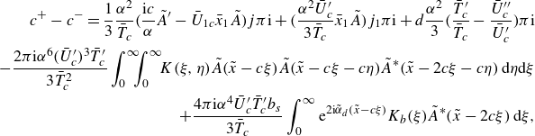 \begin{align} c^{+}-c^{-}=\frac {1}{3}\frac {\alpha ^2}{\bar {T}_c} \bigg ( \frac {\textrm{i} c}{\alpha }\tilde {A}^\prime -{\bar {U}}_{1c}\bar {x}_1 \tilde {A} \bigg )j\pi \textrm{i} +\bigg ( \frac {\alpha ^2\bar {U}_c^\prime }{3\bar {T}_c}\bar {x}_1 \tilde {A} \bigg )j_1\pi \textrm{i} +d\frac {\alpha ^2}{3}\bigg ( \frac {\bar {T}_c^\prime }{\bar {T}_c}-\frac {\bar {U}_c^{\prime \prime }}{\bar {U}_c^\prime } \bigg )\pi \textrm{i}\nonumber \\ -\frac {2\pi \textrm{i}\alpha ^6(\bar {U}_c^\prime )^3\bar {T}_c^\prime }{3\bar {T}_c^2} \int _{0}^{\infty }\!\!\!\int _{0}^{\infty }\!\! K(\xi ,\eta )\tilde {A}(\tilde {x}-c\xi ) \tilde {A}(\tilde {x}-c\xi -c\eta )\tilde {A}^*(\tilde {x}-2c\xi -c\eta )\,\textrm {d}\eta \textrm {d}\xi\nonumber \\ +\frac {4\pi \textrm{i}\alpha ^4\bar {U}_c^\prime \bar {T}_c^\prime b_s}{3\bar {T}_c} \int _{0}^{\infty } {\textrm{e}}^{2\textrm{i}\tilde {\alpha }_d(\tilde {x}-c\xi )} K_b(\xi )\tilde {A}^*(\tilde {x}-2c\xi )\,\textrm {d}\xi , \end{align}
where the linear part of the jump corresponds to the $(-\pi )$
phase jump of the logarithmic singularity in (3.15), and the kernel functions
$(-\pi )$
phase jump of the logarithmic singularity in (3.15), and the kernel functions
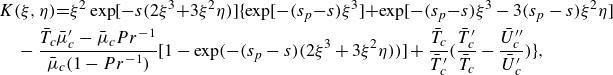 \begin{align} & K(\xi ,\eta )\!=\!\xi ^2\exp [-s(2\xi ^3\!+\!3\xi ^2\eta )]\bigg \{ \!\exp [-(s_p\!-\!s)\xi ^3]\! +\!\exp [-(s_p\!-\!s)\xi ^3-3(s_p-s)\xi ^2\eta ]\nonumber \\ & \quad -\frac {\bar {T}_c\bar {\mu }_c^\prime -\bar {\mu }_c Pr^{-1}}{\bar {\mu }_c(1-Pr^{-1})} \Big [ 1-\exp (-(s_p-s)(2\xi ^3+3\xi ^2\eta )) \Big ] +\frac {\bar {T}_c}{\bar {T}_c^\prime }\bigg ( \frac {\bar {T}_c^\prime }{\bar {T}_c}-\frac {\bar {U}_c^{\prime \prime }}{\bar {U}_c^\prime } \bigg ) \bigg \}, \\[-12pt]\nonumber \end{align}
 \begin{align} & K_b(\xi )=\xi {\textrm{e}}^{-2s\xi ^3}\bigg \{ {\textrm{e}}^{-(s_p-s)\xi ^3} -\frac {\bar {T}_c\bar {\mu }_c^\prime -\bar {\mu }_c Pr^{-1}}{\bar {\mu }_c(1-Pr^{-1})}\Big [ 1-{\textrm{e}}^{-2(s_p-s)\xi ^3} \Big ] +\frac {\bar {T}_c}{\bar {T}_c^\prime }\bigg ( \frac {\bar {T}_c^\prime }{\bar {T}_c}-\frac {\bar {U}_c^{\prime \prime }}{\bar {U}_c^\prime } \bigg ) \bigg \}.\end{align}
The last term in (3.42) is contributed by the subharmonic parametric resonance between the radiating mode and the boundary-layer response to the incident wave.
Inserting the jumps (3.31) and (3.42) into (3.19), we obtain the evolution equation for the amplitude function $\tilde {A}$
(cf. Qin & Wu Reference Qin and Wu2024),
$\tilde {A}$
(cf. Qin & Wu Reference Qin and Wu2024),
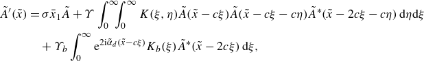 \begin{align} \tilde {A}^\prime (\tilde {x})& =\sigma \bar {x}_1 \tilde {A}+\Upsilon \int _{0}^{\infty }\!\!\!\int _{0}^{\infty } K(\xi ,\eta ) \tilde {A}(\tilde {x}-c\xi )\tilde {A}(\tilde {x}-c\xi -c\eta )\tilde {A}^*(\tilde {x}-2c\xi -c\eta )\,\textrm {d}\eta \textrm {d}\xi\nonumber \\ & \quad +\Upsilon _b\int _{0}^{\infty } {\textrm{e}}^{2\textrm{i}\tilde {\alpha }_d(\tilde {x}-c\xi )} K_b(\xi )\tilde {A}^*(\tilde {x}-2c\xi )\,\textrm {d}\xi , \end{align}
where
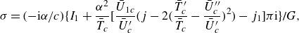 \begin{equation} \sigma =(-\textrm{i}\alpha /c)\bigg \{ I_1+\frac {\alpha ^2}{\bar {T}_c} \bigg [ \frac {{\bar {U}}_{1c}}{\bar {U}_c^\prime } \bigg ( j-2\bigg ( \frac {\bar {T}_c^\prime }{\bar {T}_c}-\frac {\bar {U}_c^{\prime \prime }}{\bar {U}_c^\prime } \bigg )^2 \bigg ) -j_1 \bigg ]\pi \textrm{i} \bigg \}\bigg /G, \end{equation}
 \begin{equation} \Upsilon =2\pi \alpha ^7(\bar {U}_c^\prime )^2\bar {T}_c^\prime /(c\bar {T}_c^2G), \qquad \Upsilon _b=-4\pi \alpha ^5\bar {T}_c^\prime b_s/(c\bar {T}_c G), \end{equation}
with $b_s=b_s(p_I)$
given by (3.32) and
$b_s=b_s(p_I)$
given by (3.32) and
 \begin{align} G=2I_2+\frac {\alpha ^2}{\bar {T}_c\bar {U}_c^\prime }\bigg [ j-2\bigg ( \frac {\bar {T}_c^\prime }{\bar {T}_c}-\frac {\bar {U}_c^{\prime \prime }}{\bar {U}_c^\prime } \bigg )^2 \bigg ]\pi \textrm{i}. \end{align}
In addition to the cubic self-nonlinear term, the amplitude equation (3.45) consists also of a linear non-local term, which accounts for the impact of the incident sound on the evolution of the radiating mode.
3.1.3. Effects of incident sound on the linear growth rate
The solution to the amplitude equation (3.45) can be written as
 \begin{equation} \tilde {A}=A_0(\tilde {x}){\textrm{e}}^{\textrm{i}\tilde \alpha _d\tilde {x}}. \end{equation}
By substituting (3.49) into (3.45), we obtain
 \begin{align} A_0^\prime (\tilde {x})& =(\kappa _{0}-\textrm{i}\tilde \alpha _d)A_0\nonumber \\ & \quad +\Upsilon \int _{0}^{\infty }\!\!\!\int _{0}^{\infty }\! K(\xi ,\eta ) A_0(\tilde {x}-c\xi )A_0(\tilde {x}-c\xi -c\eta )A_0^*(\tilde {x}-2c\xi -c\eta )\,\textrm {d}\eta \textrm {d}\xi \nonumber \\ & \quad +\Upsilon _b\int _{0}^{\infty }\! K_b(\xi )A_0^*(\tilde {x}-2c\xi )\,\textrm {d}\xi , \end{align}
where we have put $\kappa _{0}=\sigma \bar {x}_1$
. In the upstream regime, where the amplitude of the radiating mode is small, the nonlinear term in (3.50) can be neglected, leading to the equation
$\kappa _{0}=\sigma \bar {x}_1$
. In the upstream regime, where the amplitude of the radiating mode is small, the nonlinear term in (3.50) can be neglected, leading to the equation
 \begin{equation} A_0^\prime (\tilde {x})=(\kappa _{0}-\textrm{i}\tilde \alpha _d)A_0 +\Upsilon _b\int _{0}^{\infty }\! K_b(\xi )A_0^*(\tilde {x}-2c\xi )\,\textrm {d}\xi \quad \mbox{as}\quad \tilde {x}\rightarrow -\infty . \end{equation}
Let us seek a solution of the form
 \begin{equation} A_0=A_{0r}+\textrm{i} A_{0i}, \qquad (A_{0r},A_{0i})=(a_r,a_i){\textrm{e}}^{\kappa \tilde {x}}+\textrm{c.c.}, \end{equation}
where $a_r$
and
$a_r$
and $a_i$
are both complex constants, and so is
$a_i$
are both complex constants, and so is $\kappa$
with its real part representing the linear growth rate modified by the incident sound. Then,
$\kappa$
with its real part representing the linear growth rate modified by the incident sound. Then, $A_0$
can be written as
$A_0$
can be written as
 \begin{equation} A_0=(a_r+\textrm{i} a_i){\textrm{e}}^{\kappa \tilde {x}}+(a_r^*+\textrm{i} a_i^*){\textrm{e}}^{\kappa ^*\tilde {x}}. \end{equation}
Substitution of (3.53) into (3.51) and collection of terms proportional to ${\textrm{e}}^{\kappa \tilde {x}}$
and
${\textrm{e}}^{\kappa \tilde {x}}$
and ${\textrm{e}}^{\kappa ^*\tilde {x}}$
lead to the eigenvalue problem,
${\textrm{e}}^{\kappa ^*\tilde {x}}$
lead to the eigenvalue problem,
 \begin{equation} \begin{pmatrix} \kappa _{0r}+\Upsilon _{br}\chi _b & -\kappa _{0i}+\tilde \alpha _d+\Upsilon _{bi}\chi _b \\ \kappa _{0i}-\tilde \alpha _d+\Upsilon _{bi}\chi _b & \kappa _{0r}-\Upsilon _{br}\chi _b \end{pmatrix} \begin{pmatrix} a_r \\ a_i \end{pmatrix}=\kappa \begin{pmatrix} a_r \\ a_i \end{pmatrix}, \end{equation}
where we have put
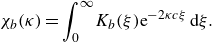 \begin{equation} \chi _b(\kappa )=\int _{0}^{\infty }\! K_b(\xi ){\textrm{e}}^{-2\kappa c\xi }\,\textrm {d}\xi . \end{equation}
The requirement for non-zero solutions $(a_r, a_i)$
gives the characteristic equation for
$(a_r, a_i)$
gives the characteristic equation for $\kappa$
,
$\kappa$
,
 \begin{equation} \mathcal{F}\equiv (\kappa -\kappa _{0r})^2+(\kappa _{0i}-\tilde \alpha _d)^2 -(|\Upsilon _{b}|\chi _{b})^2=0. \end{equation}
The function $\mathcal{F}$
is real if
$\mathcal{F}$
is real if $\kappa$
is, and thus if the equation
$\kappa$
is, and thus if the equation $\mathcal{F}=0$
admits a complex root
$\mathcal{F}=0$
admits a complex root $\kappa$
, so is its complex conjugate. The equation is solved numerically using Newton iteration. The corresponding eigenvector
$\kappa$
, so is its complex conjugate. The equation is solved numerically using Newton iteration. The corresponding eigenvector $(a_r, a_i)$
is obtained from (3.54) and written as
$(a_r, a_i)$
is obtained from (3.54) and written as
 \begin{equation} a_r=a_0 a_{r0}\equiv |a_0||a_{r0}|{\textrm{e}}^{\textrm{i}(\theta _1+\phi _0)}, \qquad a_i=a_0 a_{i0}\equiv |a_0||a_{i0}|{\textrm{e}}^{\textrm{i}(\theta _2+\phi _0)}, \end{equation}
where $(a_r, a_i)$
is normalised such that
$(a_r, a_i)$
is normalised such that $|a_{r0}|^2+|a_{i0}|^2=1$
, and
$|a_{r0}|^2+|a_{i0}|^2=1$
, and $a_0=|a_0|{\textrm{e}}^{\textrm{i}\phi _0}$
is a complex constant. Thus, the perturbation
$a_0=|a_0|{\textrm{e}}^{\textrm{i}\phi _0}$
is a complex constant. Thus, the perturbation $A_0$
can be written as
$A_0$
can be written as
 \begin{equation} A_0=2|a_0|{\textrm{e}}^{\kappa _r\tilde {x}}\Big [ |a_{r0}|\cos (\kappa _i\tilde {x}+\theta _1+\phi _0) +\textrm{i}|a_{i0}|\cos (\kappa _i\tilde {x}+\theta _2+\phi _0) \Big ]. \end{equation}
The coefficient of the subharmonic resonance term in (3.45) is proportional to $b_s$
, which depends on
$b_s$
, which depends on $p_I$
. We now estimate its values pertinent to applications. The noise level
$p_I$
. We now estimate its values pertinent to applications. The noise level $\tilde {p}_s$
in conventional wind tunnels is of
$\tilde {p}_s$
in conventional wind tunnels is of $O(10^{-3})$
(Masutti et al. Reference Masutti, Spinosa, Chazot and Carbonaro2012; Cerminara et al. Reference Cerminara, Durant, André, Sandham and Taylor2019), but in flight conditions, it can be one to two orders of magnitude lower (Schneider Reference Schneider2008, Reference Schneider2015). Thus, we estimate that
$O(10^{-3})$
(Masutti et al. Reference Masutti, Spinosa, Chazot and Carbonaro2012; Cerminara et al. Reference Cerminara, Durant, André, Sandham and Taylor2019), but in flight conditions, it can be one to two orders of magnitude lower (Schneider Reference Schneider2008, Reference Schneider2015). Thus, we estimate that $\tilde {p}_s=O(10^{-4})$
. Typical Reynolds numbers are in the range of
$\tilde {p}_s=O(10^{-4})$
. Typical Reynolds numbers are in the range of $10^4$
–
$10^4$
– $10^5$
. Recall that the pressure of the acoustic wave takes the form
$10^5$
. Recall that the pressure of the acoustic wave takes the form $\tilde {p}_s=\tilde \epsilon _s p_I{\textrm{e}}^{\textrm{i}(\alpha _{s}{x}+\gamma _{s}{y}-\omega _{s}{t})}+\textrm{c.c.}$
It follows that
$\tilde {p}_s=\tilde \epsilon _s p_I{\textrm{e}}^{\textrm{i}(\alpha _{s}{x}+\gamma _{s}{y}-\omega _{s}{t})}+\textrm{c.c.}$
It follows that

Effects on $\kappa$
of the impinging sound intensity with
$\kappa$
of the impinging sound intensity with $\tilde \alpha _d=-1$
and
$\tilde \alpha _d=-1$
and $\lambda =1$
: (
$\lambda =1$
: ( $a$
)
$a$
) $\kappa _r$
and (
$\kappa _r$
and ( $b$
)
$b$
) $\kappa _i$
. The dashed line represents the linear growth rate in the absence of the incident sound.
$\kappa _i$
. The dashed line represents the linear growth rate in the absence of the incident sound.
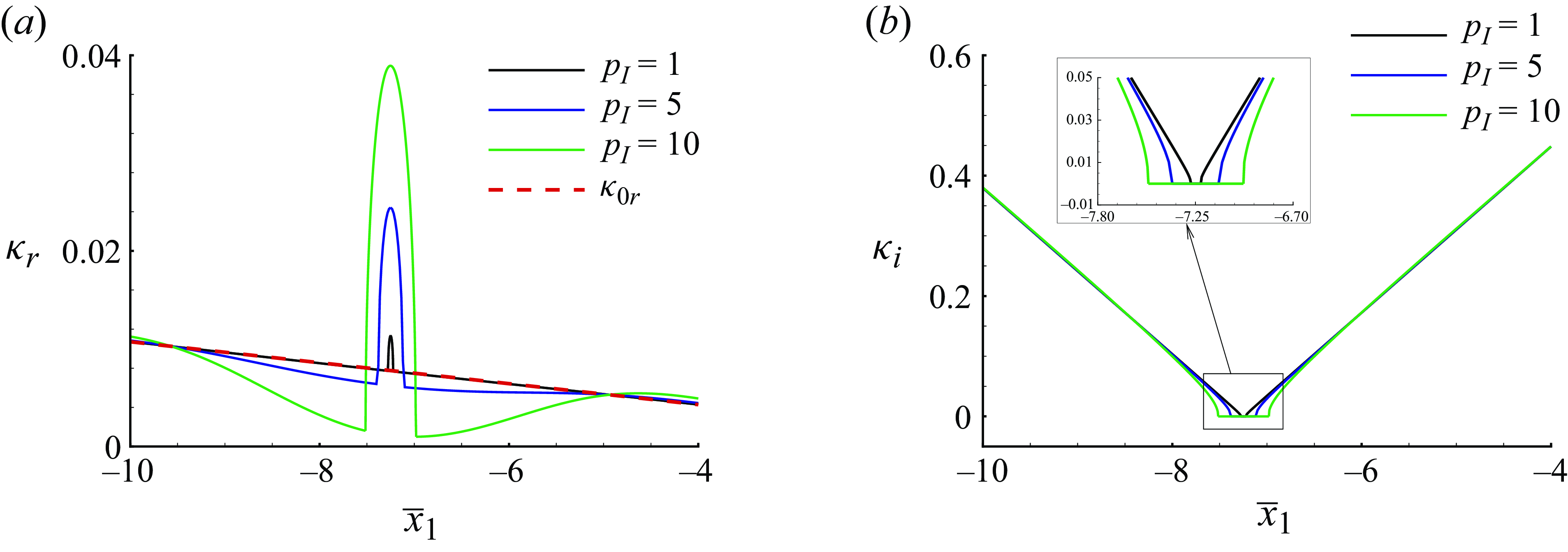
Effects on $\kappa$
of the detuning with
$\kappa$
of the detuning with $p_I=5$
and
$p_I=5$
and $\lambda =1$
: (
$\lambda =1$
: ( $a$
)
$a$
) $\kappa _r$
and (
$\kappa _r$
and ( $b$
)
$b$
) $\kappa _i$
. The dashed line represents the linear growth rate in the absence of the incident sound.
$\kappa _i$
. The dashed line represents the linear growth rate in the absence of the incident sound.
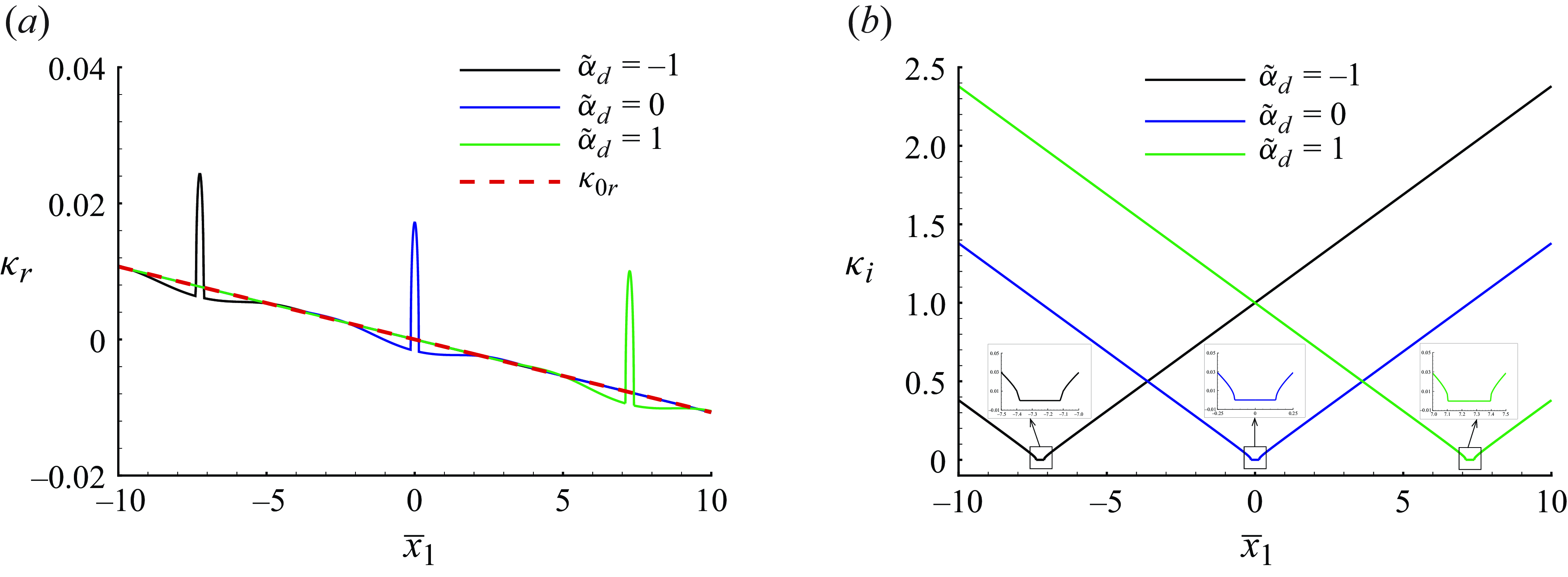
Figure 2 shows the effects of $p_I$
on the modified growth rate
$p_I$
on the modified growth rate $\kappa _r$
. Depending on the position
$\kappa _r$
. Depending on the position $\bar {x}_1$
and the detuned parameter
$\bar {x}_1$
and the detuned parameter $\tilde \alpha _d$
,
$\tilde \alpha _d$
, $\kappa _r$
is either enhanced or reduced by the impinging sound. The modified growth rate increases with
$\kappa _r$
is either enhanced or reduced by the impinging sound. The modified growth rate increases with $p_I$
in a narrow region corresponding to a moderate range of
$p_I$
in a narrow region corresponding to a moderate range of $\bar {x}_1$
, beyond which it decreases with
$\bar {x}_1$
, beyond which it decreases with $p_I$
over a broader range, suggesting that the sound plays a stabilising role. As
$p_I$
over a broader range, suggesting that the sound plays a stabilising role. As $|\bar {x}_1|\rightarrow \infty$
,
$|\bar {x}_1|\rightarrow \infty$
, $\kappa _r$
approaches the unperturbed growth rate
$\kappa _r$
approaches the unperturbed growth rate $\kappa _{0r}$
. This can be inferred by examining (3.56). Since
$\kappa _{0r}$
. This can be inferred by examining (3.56). Since $\kappa _{0r}$
and
$\kappa _{0r}$
and $\kappa _{0i}$
are proportional to
$\kappa _{0i}$
are proportional to $\bar {x}_1$
, the dominant balance for large
$\bar {x}_1$
, the dominant balance for large $|\bar {x}_1|$
yields
$|\bar {x}_1|$
yields $(\kappa -\kappa _{0r})^2+(\kappa _{0i}-\tilde {\alpha }_d)^2=0$
so that
$(\kappa -\kappa _{0r})^2+(\kappa _{0i}-\tilde {\alpha }_d)^2=0$
so that $\kappa _r=\kappa _{0r}$
and
$\kappa _r=\kappa _{0r}$
and $\kappa _i=\pm (\kappa _{0i}-\tilde {\alpha }_d)$
. Since the function
$\kappa _i=\pm (\kappa _{0i}-\tilde {\alpha }_d)$
. Since the function $\mathcal{F}$
is real for real values of
$\mathcal{F}$
is real for real values of $\kappa$
, it may admit real roots for certain parameters. Indeed, the solution changes from a complex conjugate pair to a single real root at certain positions, as is shown by the trend of
$\kappa$
, it may admit real roots for certain parameters. Indeed, the solution changes from a complex conjugate pair to a single real root at certain positions, as is shown by the trend of $\kappa _i$
in figure 2(
$\kappa _i$
in figure 2( $b$
). Destabilising effect of the subharmonic resonance is observed primarily in the regions where
$b$
). Destabilising effect of the subharmonic resonance is observed primarily in the regions where $\kappa$
is real. As
$\kappa$
is real. As $p_I$
increases to a high value, the range over which the acoustic wave destabilises the radiating mode broadens, and the peak modified growth rate becomes significantly larger. These trends align with the behaviour illustrated in figure 2(
$p_I$
increases to a high value, the range over which the acoustic wave destabilises the radiating mode broadens, and the peak modified growth rate becomes significantly larger. These trends align with the behaviour illustrated in figure 2( $a$
). Figure 3 shows the variation of the modified growth rate with
$a$
). Figure 3 shows the variation of the modified growth rate with $\bar {x}_1$
for three values of
$\bar {x}_1$
for three values of $\tilde \alpha _d$
. Altering
$\tilde \alpha _d$
. Altering $\tilde \alpha _d$
shifts the distribution of both
$\tilde \alpha _d$
shifts the distribution of both $\kappa _r$
and
$\kappa _r$
and $\kappa _i$
. Again, the complex roots
$\kappa _i$
. Again, the complex roots $\kappa$
develop into real roots in a narrow region in each case. All these results indicate that for the parameters examined, the impinging sound in general weakens slightly the linear development of the radiating mode, but in a small region, it enhances significantly the modal growth.
$\kappa$
develop into real roots in a narrow region in each case. All these results indicate that for the parameters examined, the impinging sound in general weakens slightly the linear development of the radiating mode, but in a small region, it enhances significantly the modal growth.
3.1.4. Nonlinear evolution
We proceed to consider effects of the impinging sound on the nonlinear development by solving numerically the nonlinear amplitude equation (3.50), subject to the appropriate initial condition (3.58) as $\tilde {x}\rightarrow -\infty$
. The six-order Adams–Moulton method is used, and the integral terms are approximated by Simpson’s rule. Results are shown in figures 4 and 5. Note that the impinging sound wave modifies the linear growth rate only slightly in the case shown in figure 4, but significantly in the case displayed in figure 5. The amplitude always develops into a singularity at a finite distance. Increasing the intensity of the sound wave advances appreciably its occurrence (figures 4
$\tilde {x}\rightarrow -\infty$
. The six-order Adams–Moulton method is used, and the integral terms are approximated by Simpson’s rule. Results are shown in figures 4 and 5. Note that the impinging sound wave modifies the linear growth rate only slightly in the case shown in figure 4, but significantly in the case displayed in figure 5. The amplitude always develops into a singularity at a finite distance. Increasing the intensity of the sound wave advances appreciably its occurrence (figures 4 $a$
and 5
$a$
and 5 $a$
). This is so even though the effect on the linear growth rate is rather limited (figure 4
$a$
). This is so even though the effect on the linear growth rate is rather limited (figure 4 $a$
). We also examine the effects of viscosity on the nonlinear development, which generally delays the occurrence of the finite-distance singularity (figures 4
$a$
). We also examine the effects of viscosity on the nonlinear development, which generally delays the occurrence of the finite-distance singularity (figures 4 $b$
and 5
$b$
and 5 $b$
), similar to what has been found previously for free-mode evolution (Goldstein & Leib Reference Goldstein and Leib1989; Leib Reference Leib1991) and for fundamental resonance with impinging sound (Qin & Wu Reference Qin and Wu2024). One may note that the solutions in figure 4 are more oscillatory than those in figure 5. This is due to the fact that linear modes in figure 4 have non-zero
$b$
), similar to what has been found previously for free-mode evolution (Goldstein & Leib Reference Goldstein and Leib1989; Leib Reference Leib1991) and for fundamental resonance with impinging sound (Qin & Wu Reference Qin and Wu2024). One may note that the solutions in figure 4 are more oscillatory than those in figure 5. This is due to the fact that linear modes in figure 4 have non-zero $\kappa _i$
, which renders the solutions oscillatory as (3.58) indicates, whereas those in figure 5 are non-oscillatory with
$\kappa _i$
, which renders the solutions oscillatory as (3.58) indicates, whereas those in figure 5 are non-oscillatory with $\kappa _i=0$
.
$\kappa _i=0$
.
Effects of incident sound intensity and viscosity on the nonlinear evolution of the radiating mode. ( $a$
) Nonlinear development for different values of
$a$
) Nonlinear development for different values of $p_I$
with
$p_I$
with $\lambda =1$
. (
$\lambda =1$
. ( $b$
) Nonlinear development for different values of
$b$
) Nonlinear development for different values of $\lambda$
with
$\lambda$
with $p_I=40$
. The dashed lines represent the corresponding linear solution (3.58). Here, we have taken
$p_I=40$
. The dashed lines represent the corresponding linear solution (3.58). Here, we have taken $\bar {x}_1=-4$
,
$\bar {x}_1=-4$
, $\tilde \alpha _d=-1$
and
$\tilde \alpha _d=-1$
and $a_0=1$
.
$a_0=1$
.
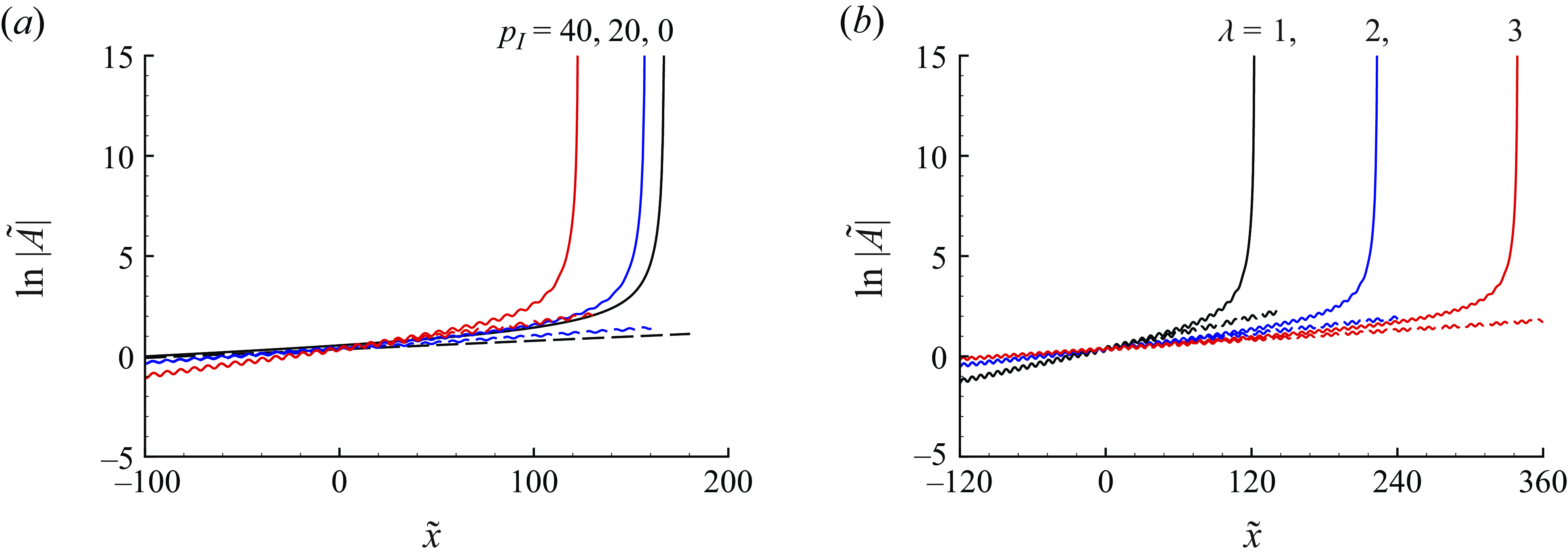
Effects of incident sound intensity and viscosity on the nonlinear evolution of the radiating mode. ( $a$
) Nonlinear development for different values of
$a$
) Nonlinear development for different values of $p_I$
with
$p_I$
with $\lambda =1$
. (
$\lambda =1$
. ( $b$
) Nonlinear development for different values of
$b$
) Nonlinear development for different values of $\lambda$
with
$\lambda$
with $p_I=10$
. The dashed lines represent the corresponding linear solution (3.58). Here, we have taken
$p_I=10$
. The dashed lines represent the corresponding linear solution (3.58). Here, we have taken $\bar {x}_1=-7.25$
,
$\bar {x}_1=-7.25$
, $\tilde \alpha _d=-1$
and
$\tilde \alpha _d=-1$
and $a_0=1$
.
$a_0=1$
.
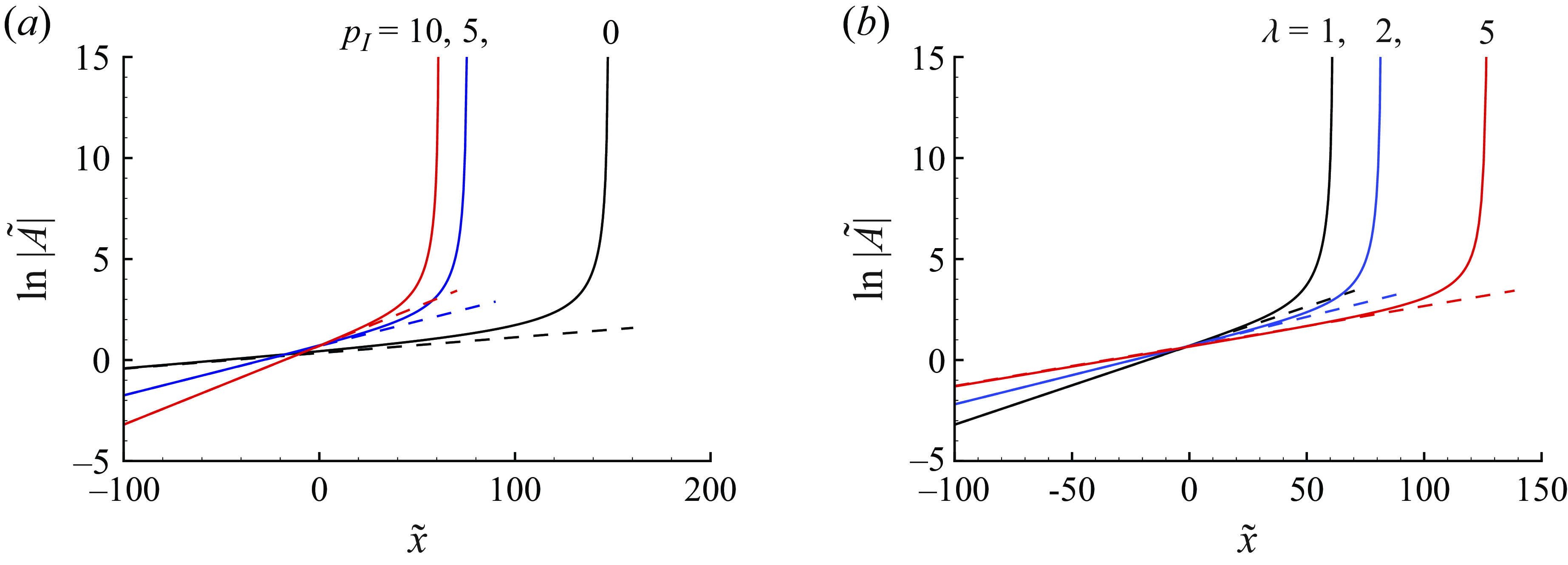
3.2. Equilibrium non-parallel regime
As was shown in § 2.3.2, a sound influences nonlinearly the evolution of the radiating mode in the equilibrium regime when its magnitude $\bar {\epsilon }_s=O(Re^{-7/6})$
, and its wavenumber/frequency is close to/the same as twice those of the radiating mode, that is,
$\bar {\epsilon }_s=O(Re^{-7/6})$
, and its wavenumber/frequency is close to/the same as twice those of the radiating mode, that is,
 \begin{equation} \alpha _{s}=2(\alpha +Re^{-1/2}\bar \alpha _d), \qquad \omega _{s}=2\omega , \end{equation}
where $\bar \alpha _d$
is an
$\bar \alpha _d$
is an $O(1)$
detuning parameter. For
$O(1)$
detuning parameter. For $Re=10^{4}\textrm{--}10^{5}$
,
$Re=10^{4}\textrm{--}10^{5}$
, $\bar {p}_I=\tilde {p}_s/\bar {\epsilon }_s=\tilde {p}_s/Re^{-7/6}\approx 4.64\textrm{--}68.13$
.
$\bar {p}_I=\tilde {p}_s/\bar {\epsilon }_s=\tilde {p}_s/Re^{-7/6}\approx 4.64\textrm{--}68.13$
.
3.2.1. Main layer
The analysis in the main layer is only slightly modified with expansion (3.2) being replaced by
 \begin{align} (\tilde \rho , \tilde {u}, \tilde {v}, \tilde {p}, \tilde \theta )&= \bar {\epsilon }\Big [ \bar {A}(\bar {x})(\hat {\rho }_0, \hat {u}_0, \hat {v}_0, \hat {p}_0, \hat {\theta }_0) +Re^{-1/2}(\hat {\rho }_1, \hat {u}_1, \hat {v}_1, \hat {p}_1, \hat {\theta }_1) \Big ]E \\ &\quad \nonumber +\,\bar \epsilon _s(\check \rho _s, \check {u}_s, \check {v}_s, \check {p}_s, \check \theta _s)E_s+\textrm{c.c.}+\cdots . \end{align}
The corresponding solvability condition (3.19) becomes
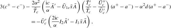 \begin{align} 3(c^{+}-c^{-})&-\frac {2\alpha ^2}{\bar {T}_c} \left ( \frac {\textrm{i} c}{\alpha }\bar {A}^\prime -{\bar {U}}_{1c}\bar {x} \bar {A} \right ) \left ( \frac {\bar {T}_c^\prime }{\bar {T}_c}-\frac {\bar {U}_c^{\prime \prime }}{\bar {U}_c^\prime } \right )(a^{+}-a^{-}) -\alpha ^2 d(a^{+}-a^{-})\nonumber \\ &\quad =-\bar {U}_c^\prime \left (\frac {2\textrm{i} c}{\alpha }I_2 \bar {A}^\prime -I_1\bar {x} \bar {A}\right ), \end{align}
which corresponds to (3.19) but with the parameter $\bar {x}_1$
being replaced by variable
$\bar {x}_1$
being replaced by variable $\bar {x}$
. The jumps
$\bar {x}$
. The jumps $(a^{+}-a^{-})$
and
$(a^{+}-a^{-})$
and $(c^{+}-c^{-})$
are determined by analysing the critical-layer dynamics.
$(c^{+}-c^{-})$
are determined by analysing the critical-layer dynamics.
3.2.2. Critical layer
The singularity in the main-layer solution is removed by reintroducing viscosity in the critical layer with an $O(Re^{-1/3})$
width, and so the appropriate local transverse coordinate is
$O(Re^{-1/3})$
width, and so the appropriate local transverse coordinate is
 \begin{equation} Y=(y-y_c)/Re^{-1/3}. \end{equation}
The perturbation expands as
 \begin{align} \tilde {u}&=\bar {\epsilon }(U_{1}E+Re^{-1/6}U_{2}E+Re^{-1/4}U_{M}+Re^{-1/2}U_{3}E) +\bar \epsilon _s U_{s1}E_s+\textrm{c.c.}+\cdots , \qquad\qquad \\[-28pt] \nonumber \end{align}
 \begin{align} \tilde {v}&=\bar {\epsilon }(V_{0}E + Re^{-1/3}V_{1}E + Re^{-1/2}V_{2}E + Re^{-7/12}V_{M} + Re^{-5/6}V_{3}E) + \bar \epsilon _s V_{s0}E_s + \textrm{c.c.} + \cdots , \quad \\[-28pt] \nonumber \end{align}
 \begin{align} \tilde {p}&=\bar {\epsilon }(P_{0}E+Re^{-1/3}P_{1}E+Re^{-1/2}P_{2}E+Re^{-5/6}P_{3}E) +\bar \epsilon _s P_{s0}E_s+\textrm{c.c.}+\cdots , \qquad\qquad \\[-28pt] \nonumber \end{align}
 \begin{align} \tilde \theta &=\bar {\epsilon }Re^{1/3}(\Theta _{1}E\!+\!Re^{-1/6}\Theta _{2}E\!+\!Re^{-1/4}\Theta _{M}\!+\!Re^{-1/2}\Theta _{3}E) \!+\!\bar \epsilon _s Re^{1/3}\Theta _{s1}E_s\!+\!\textrm{c.c.}\!+\!\cdots . \\[-1pt] \nonumber \end{align}
Substituting (3.64) into (2.2) and noting (2.28) and (3.63), we then obtain the equations governing the terms at different orders in the expansion.
At leading order, inspection of the $x$
-momentum and
$x$
-momentum and $y$
-momentum equations gives
$y$
-momentum equations gives
 \begin{equation} P_0=(\bar {U}_c^\prime /\bar {T}_c)\bar {A}, \qquad V_0=-\textrm{i}\alpha \bar {A}. \end{equation}
Expansion of the energy equation shows that
 \begin{equation} \bar {\mathscr{L}}_p\Theta _{1}+{\bar {T}_c^\prime }V_{0}=0, \end{equation}
where the operator $\bar {\mathscr{L}}_p$
is defined by
$\bar {\mathscr{L}}_p$
is defined by
 \begin{equation} \bar {\mathscr{L}}_p=\textrm{i}\alpha \bar {U}_c^\prime Y-\bar {T}_c\bar {\mu }_c Pr^{-1}\frac {\partial ^2}{\partial Y^2}. \end{equation}
Equation (3.66) is solved by use of Fourier transform to give
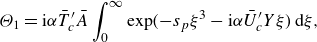 \begin{equation} \Theta _1=\textrm{i}\alpha {\bar {T}_c^\prime }\bar {A} \int _{0}^{\infty } \exp (-s_p\xi ^3-\textrm{i}\alpha \bar {U}_c^\prime Y\xi )\,\textrm {d}\xi , \end{equation}
where $s_p$
is the same as that given in (3.28) provided that
$s_p$
is the same as that given in (3.28) provided that $\lambda$
is set to unity.
$\lambda$
is set to unity.
At the next order, expansion of the continuity and $x$
-momentum equations yields two coupled equations for
$x$
-momentum equations yields two coupled equations for $U_1$
and
$U_1$
and $V_1$
. These equations are combined to obtain an equation for
$V_1$
. These equations are combined to obtain an equation for $U_{1,Y}$
, which is solved to give
$U_{1,Y}$
, which is solved to give
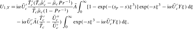 \begin{align} U_{1,Y}&=\textrm{i}\alpha \bar {U}_c^\prime \frac {\bar {T}_c^\prime (\bar {T}_c\bar {\mu }_c^\prime -\bar {\mu }_c Pr^{-1})}{\bar {T}_c\bar {\mu }_c(1-Pr^{-1})}\bar {A}\! \int _{0}^{\infty } [1-\exp (-(s_p-s)\xi ^3)]\exp (-s\xi ^3-\textrm{i}\alpha \bar {U}_c^\prime Y\xi )\,\textrm {d}\xi\nonumber \\ &\quad -\textrm{i}\alpha \bar {U}_c^\prime \bar {A}\bigg ( \frac {\bar {T}_c^\prime }{\bar {T}_c}-\frac {\bar {U}_c^{\prime \prime }}{\bar {U}_c^\prime } \bigg ) \int _{0}^{\infty } \exp (-s\xi ^3-\textrm{i}\alpha \bar {U}_c^\prime Y\xi )\,\textrm {d}\xi , \end{align}
where $s$
is the same as that given in (3.30) provided that
$s$
is the same as that given in (3.30) provided that $\lambda$
is set to unity. Matching
$\lambda$
is set to unity. Matching $U_1$
with its outer counterpart determines the jump, which is the same as (3.31) (as expected).
$U_1$
with its outer counterpart determines the jump, which is the same as (3.31) (as expected).
The acoustic signature is the same as that given in § 3.1.2 provided that $\lambda$
is set to unity. The pressure, wall-normal velocity, temperature and streamwise velocity components of the acoustic disturbance are given by (3.32), (3.34a
), (3.34b
) and (3.37), respectively.
$\lambda$
is set to unity. The pressure, wall-normal velocity, temperature and streamwise velocity components of the acoustic disturbance are given by (3.32), (3.34a
), (3.34b
) and (3.37), respectively.
Further analysis of the critical layer is related to Appendix B.2, where we present at quadratic order the solution for the mean-flow distortion, and at the cubic level, the jump $(c^{+}-c^{-})$
is determined and given by (B10).
$(c^{+}-c^{-})$
is determined and given by (B10).
Inserting the jumps (3.31) and (B10) into (3.62), we obtain the amplitude equation for $\bar {A}$
(cf. Qin & Wu Reference Qin and Wu2024),
$\bar {A}$
(cf. Qin & Wu Reference Qin and Wu2024),
 \begin{equation} \bar {A}^\prime (\bar {x})=\sigma \bar {x}\bar {A}+l\bar {A}|\bar {A}|^2 +l_b\bar {A}^*{\textrm{e}}^{2\textrm{i}\bar \alpha _d\bar {x}}, \end{equation}
where $\sigma$
is given in (3.46), and
$\sigma$
is given in (3.46), and
 \begin{equation} l=\textrm{i}\alpha \Lambda /(c\bar {U}_c^\prime G), \qquad l_b=\textrm{i}\alpha \Lambda _b/(c\bar {U}_c^\prime G). \end{equation}
As expected, both the self-nonlinearity and the subharmonic resonance terms are now local. The amplitude equation (3.70) describes the nonlinear evolution of the radiating mode under the influence of the incident sound in the regime where non-parallelism is important.
4. Non-parallelism and the composite amplitude equation
The amplitude equations derived in the non-equilibrium parallel and equilibrium non-parallel regimes are pertinent to the two distinguished intensities of the impinging sound wave, and their respective validity regions and the associated length scales of evolution are shown in figure 6. The two regimes are connected with each other via an intermediate one that operates as the sound intensity $\tilde \epsilon _s$
is varied between the distinguished levels
$\tilde \epsilon _s$
is varied between the distinguished levels $O(Re^{-1})$
and
$O(Re^{-1})$
and $O(Re^{-7/6})$
. We now construct, by following the same consideration as Wu & Huerre (Reference Wu and Huerre2009) and Qin & Wu (Reference Qin and Wu2024), a composite amplitude equation that accounts for both the non-equilibrium and non-parallelism effects, and accommodates all the regimes including the intermediate one.
$O(Re^{-7/6})$
. We now construct, by following the same consideration as Wu & Huerre (Reference Wu and Huerre2009) and Qin & Wu (Reference Qin and Wu2024), a composite amplitude equation that accounts for both the non-equilibrium and non-parallelism effects, and accommodates all the regimes including the intermediate one.
A sketch illustrating different evolution regimes.
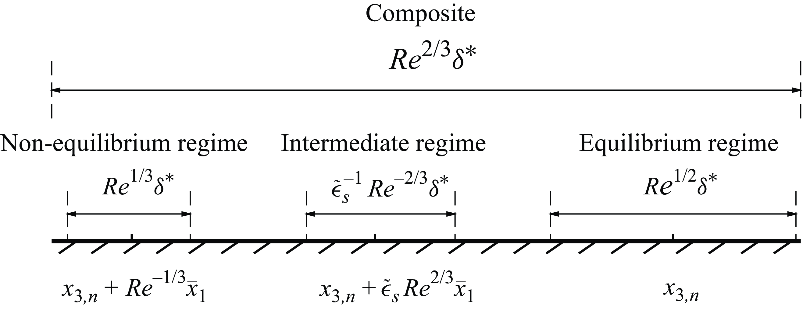
4.1. Construction of the composite amplitude equation
Recall that in the equilibrium regime, the evolution occurs in the vicinity of the neutral position (figure 6)
 \begin{equation} x_3=x_{3,n}+Re^{-1/2}\bar {x} \quad \mbox{with}\quad \bar {x}=O(1), \end{equation}
and the amplitude equation is (3.70) with $\bar \alpha _d$
being defined by (3.60). However, in the non-equilibrium regime, the evolution occurs in the vicinity of the neutral position
$\bar \alpha _d$
being defined by (3.60). However, in the non-equilibrium regime, the evolution occurs in the vicinity of the neutral position
 \begin{equation} x_3\approx x_{3,n}+Re^{-1/3}\bar {x}_1 \quad \mbox{with}\quad \bar {x}_1=O(1), \end{equation}
and the amplitude is governed by (3.45) with $\tilde \alpha _d$
being specified by (3.1).
$\tilde \alpha _d$
being specified by (3.1).
Let us first construct the composite amplitude equation starting from the non-equilibrium regime. Noting (2.21), i.e.
 \begin{equation} \tilde {x}=Re^{2/3}(x_3-(x_{3,n}+Re^{-1/3}\bar {x}_1)), \end{equation}
we can approximate the base flow by
 \begin{equation} ({\bar {U}}(x_3, y), {\bar {T}}(x_3, y)) \approx ({\bar {U}}(x_{3,n}, y), {\bar {T}}(x_{3,n}, y)) +Re^{-1/3}({\bar {U}}_1(y), {\bar {T}}_1(y))(\bar {x}_1+Re^{-1/3}\tilde {x}). \end{equation}
Following Wu & Huerre (Reference Wu and Huerre2009), we construct a composite amplitude equation by retaining the $O(Re^{-2/3})$
term in (4.4) so that the first term on the right-hand side of (3.45) is modified to
$O(Re^{-2/3})$
term in (4.4) so that the first term on the right-hand side of (3.45) is modified to $\sigma (\bar {x}_1+Re^{-1/3}\tilde {x})$
, and the exponential involving
$\sigma (\bar {x}_1+Re^{-1/3}\tilde {x})$
, and the exponential involving $\tilde {x}$
in the last term becomes
$\tilde {x}$
in the last term becomes ${\textrm{e}}^{2\textrm{i}\tilde \alpha _d(\tilde {x}+Re^{1/3}\bar {x}_1+Re^{2/3}x_{3,n})}$
.
${\textrm{e}}^{2\textrm{i}\tilde \alpha _d(\tilde {x}+Re^{1/3}\bar {x}_1+Re^{2/3}x_{3,n})}$
.
From (4.1) and (4.3), it follows that
 \begin{equation} \bar {x}=Re^{1/6}\bar {x}_1+Re^{-1/6}\tilde {x}. \end{equation}
Note that in the equilibrium regime, we expanded the perturbation as
 \begin{equation} p=\bar {\epsilon }[\bar {A}(\bar {x})\hat {p}_0+Re^{-1/2}\hat {p}_1+\cdots ], \end{equation}
where $\bar {\epsilon }=Re^{-11/12}$
, and the threshold intensity of the sound is
$\bar {\epsilon }=Re^{-11/12}$
, and the threshold intensity of the sound is $\bar {\epsilon }_s=Re^{-7/6}$
with
$\bar {\epsilon }_s=Re^{-7/6}$
with $\bar {p}_I=\tilde {p}_s/\bar {\epsilon }_s$
, whilst in the non-equilibrium regime, we expanded the perturbation as
$\bar {p}_I=\tilde {p}_s/\bar {\epsilon }_s$
, whilst in the non-equilibrium regime, we expanded the perturbation as
 \begin{equation} p=\tilde {\epsilon }[\tilde {A}(\tilde {x})\hat {p}_0+Re^{-1/3}\hat {p}_1+\cdots ], \end{equation}
where $\tilde {\epsilon }=Re^{-5/6}$
, and the threshold intensity of the sound is
$\tilde {\epsilon }=Re^{-5/6}$
, and the threshold intensity of the sound is $\tilde {\epsilon }_s=Re^{-1}$
with
$\tilde {\epsilon }_s=Re^{-1}$
with $p_I=\tilde {p}_s/\tilde {\epsilon }_s$
. Thus, we have the relations
$p_I=\tilde {p}_s/\tilde {\epsilon }_s$
. Thus, we have the relations $\bar {A}(\bar {x})=Re^{1/12}\tilde {A}(\tilde {x})$
and
$\bar {A}(\bar {x})=Re^{1/12}\tilde {A}(\tilde {x})$
and $\bar {p}_I=Re^{1/6}p_I$
(
$\bar {p}_I=Re^{1/6}p_I$
( $\bar {b}_s=Re^{1/6}b_s$
). On using these relations as well as (4.5), and noting
$\bar {b}_s=Re^{1/6}b_s$
). On using these relations as well as (4.5), and noting $\bar {\alpha }_d=Re^{1/6}\tilde \alpha _d$
, the amplitude equation (3.45) is rewritten as
$\bar {\alpha }_d=Re^{1/6}\tilde \alpha _d$
, the amplitude equation (3.45) is rewritten as
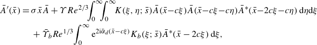 \begin{align} \bar {A}^\prime (\bar {x}) &= \sigma \bar {x}\bar {A} +\Upsilon Re^{2/3}\!\!\int _{0}^{\infty }\!\!\!\int _{0}^{\infty }\!\! K(\xi ,\eta ;\bar {s}) \bar {A}(\bar {x}\!-\!c\xi )\bar {A}(\bar {x}\!-\!c\xi\! -\!c\eta )\bar {A}^*(\bar {x}\!-\!2c\xi\! -\!c\eta )\,\textrm {d}\eta \textrm {d}\xi\nonumber \\ &\quad \, +\bar \Upsilon _b Re^{1/3}\!\int _{0}^{\infty } {\textrm{e}}^{2\textrm{i}\bar \alpha _d(\bar {x}-c\xi )} K_b(\xi ;\bar {s})\bar {A}^*(\bar {x}-2c\xi )\,\textrm {d}\xi , \end{align}
where $\bar {s}=sRe^{1/2}$
and
$\bar {s}=sRe^{1/2}$
and $\bar \Upsilon _b=\bar \Upsilon _b(\bar {p}_I)$
given by (3.47), and we have taken
$\bar \Upsilon _b=\bar \Upsilon _b(\bar {p}_I)$
given by (3.47), and we have taken $x_{3,n}=0$
without loss of generality.
$x_{3,n}=0$
without loss of generality.
The same composite amplitude equation may alternatively be constructed starting from the equilibrium regime by retaining the small non-equilibrium term in the critical-layer operator, which then becomes
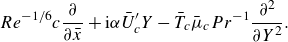 \begin{equation} Re^{-1/6}c\frac {\partial }{\partial \bar {x}} +\textrm{i}\alpha \bar {U}_c^\prime Y-\bar {T}_c\bar {\mu }_c Pr^{-1}\frac {\partial ^2}{\partial Y^2}. \end{equation}
In Appendix C, we show that the evolution problems in the equilibrium and non-equilibrium regimes can be properly recovered from the composite theory.
The initial condition for the composite amplitude equation (4.8) is obtained by neglecting the nonlinear term, leading to
 \begin{equation} \bar {A}^\prime (\bar {x})=\sigma \bar {x}\bar {A} +\bar \Upsilon _b Re^{1/3}\int _{0}^{\infty } {\textrm{e}}^{2\textrm{i}\bar \alpha _d(\bar {x}-c\xi )} K_b(\xi ;\bar {s})\bar {A}^*(\bar {x}-2c\xi )\,\textrm {d}\xi \quad \mbox{as}\quad \bar {x}\rightarrow -\infty . \end{equation}
It appears impossible to find an analytical solution to this equation, but we can seek the solution in the form of an approximation. To this end, we write $\bar {A}$
as
$\bar {A}$
as
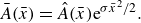 \begin{equation} \bar {A}(\bar {x})=\hat {A}(\bar {x}){\textrm{e}}^{\sigma \bar {x}^2/2}. \end{equation}
Equation (4.10) reduces to
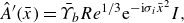 \begin{equation} \hat {A}^\prime (\bar {x})=\bar \Upsilon _b Re^{1/3}{\textrm{e}}^{-\textrm{i}\sigma _i\bar {x}^2} I, \end{equation}
where $I$
is defined by
$I$
is defined by
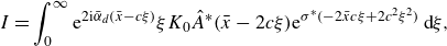 \begin{equation} I=\int _{0}^{\infty } {\textrm{e}}^{2\textrm{i}\bar \alpha _d(\bar {x}-c\xi )} \xi K_0\hat {A}^*(\bar {x}-2c\xi ){\textrm{e}}^{\sigma ^*(-2\bar {x}c\xi +2c^2\xi ^2)}\,\textrm {d}\xi , \end{equation}
and we have put $K_0=K_b/\xi$
. Performing the substitution
$K_0=K_b/\xi$
. Performing the substitution $\bar \xi =-2\bar {x}c\xi$
in the integral
$\bar \xi =-2\bar {x}c\xi$
in the integral $I$
and taking the limit
$I$
and taking the limit $\bar {x}\rightarrow -\infty$
lead to
$\bar {x}\rightarrow -\infty$
lead to
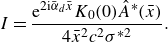 \begin{equation} I=\frac {{\textrm{e}}^{2\textrm{i}\bar \alpha _d\bar {x}}K_0(0)\hat {A}^*(\bar {x})}{4\bar {x}^2c^2\sigma ^{*2}}. \end{equation}
We expand $\hat {A}=\breve {a}_0+\hat {A}_1+\cdots$
, where
$\hat {A}=\breve {a}_0+\hat {A}_1+\cdots$
, where $\hat {A}_1$
is a small correction. Substitution of this expansion along with (4.14) into (4.12) gives
$\hat {A}_1$
is a small correction. Substitution of this expansion along with (4.14) into (4.12) gives
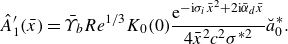 \begin{equation} \hat {A}_1^\prime (\bar {x})=\bar \Upsilon _b Re^{1/3}K_0(0) \frac {{\textrm{e}}^{-\textrm{i}\sigma _i\bar {x}^2+2\textrm{i}\bar \alpha _d\bar {x}}} {4\bar {x}^2c^2\sigma ^{*2}}\breve {a}_0^*. \end{equation}
The solution is found to be
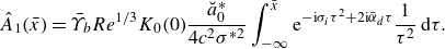 \begin{equation} \hat {A}_1(\bar {x})=\bar \Upsilon _b Re^{1/3}K_0(0)\frac {\breve {a}_0^*}{4c^2\sigma ^{*2}} \int _{-\infty }^{\bar {x}} {\textrm{e}}^{-\textrm{i}\sigma _i\tau ^2+2\textrm{i}\bar \alpha _d\tau } \frac {1}{\tau ^2}\,\textrm {d}\tau . \end{equation}
As $\bar {x}\rightarrow -\infty$
, integration by parts yields the asymptotic approximation
$\bar {x}\rightarrow -\infty$
, integration by parts yields the asymptotic approximation
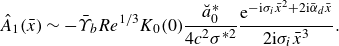 \begin{equation} \hat {A}_1(\bar {x})\sim -\bar \Upsilon _b Re^{1/3}K_0(0)\frac {\breve {a}_0^*}{4c^2\sigma ^{*2}} \frac {{\textrm{e}}^{-\textrm{i}\sigma _i\bar {x}^2+2\textrm{i}\bar \alpha _d\bar {x}}}{2\textrm{i}\sigma _i\bar {x}^3}. \end{equation}
Therefore, the initial condition for the composite amplitude equation (4.8) reads
 \begin{equation} \bar {A}(\bar {x})={\textrm{e}}^{\sigma \bar {x}^2/2}\bigg \{ \breve {a}_0-\bar \Upsilon _b Re^{1/3}K_0(0)\frac {\breve {a}_0^*}{4c^2\sigma ^{*2}} \frac {{\textrm{e}}^{-\textrm{i}\sigma _i\bar {x}^2+2\textrm{i}\bar \alpha _d\bar {x}}}{2\textrm{i}\sigma _i\bar {x}^3} +\cdots \bigg \} \quad \mbox{as}\quad \bar {x}\rightarrow -\infty . \end{equation}
It is worth noting that the second term on the right-hand side of (4.18) is tied to the amplitude of the incoming acoustic wave since $\bar \Upsilon _b$
is a function of
$\bar \Upsilon _b$
is a function of $\bar {p}_I$
(see (3.47)).
$\bar {p}_I$
(see (3.47)).
4.2. Numerical results
The composite amplitude equation (4.8) is solved numerically for a moderate value of $\bar {p}_I$
using the same method as that for (3.45). A resolution check is performed first, where two grid sizes are employed. The results overlap to graphical accuracy as is shown in figure 7, indicating a satisfactory accuracy.
$\bar {p}_I$
using the same method as that for (3.45). A resolution check is performed first, where two grid sizes are employed. The results overlap to graphical accuracy as is shown in figure 7, indicating a satisfactory accuracy.
To see how nonlinearity affects the solutions in the presence of sound, we fix $\bar {p}_I=40$
and vary the initial amplitude
$\bar {p}_I=40$
and vary the initial amplitude $\breve {a}_0$
when solving (4.8) subject to the initial condition (4.18). The results are displayed in figure 8. As expected, there is little difference between the linear and nonlinear solution for small initial amplitude
$\breve {a}_0$
when solving (4.8) subject to the initial condition (4.18). The results are displayed in figure 8. As expected, there is little difference between the linear and nonlinear solution for small initial amplitude $\breve {a}_0=1$
(figure 8
$\breve {a}_0=1$
(figure 8 $a$
). As the initial magnitude of
$a$
). As the initial magnitude of $\breve {a}_0$
increases, nonlinear effects are no longer negligible. For
$\breve {a}_0$
increases, nonlinear effects are no longer negligible. For $\breve {a}_0=3$
, the nonlinear and linear solutions are qualitatively similar, but there is appreciable quantitative difference with the amplitude acquiring a larger value under the influence of nonlinearity (figure 8
$\breve {a}_0=3$
, the nonlinear and linear solutions are qualitatively similar, but there is appreciable quantitative difference with the amplitude acquiring a larger value under the influence of nonlinearity (figure 8 $b$
). A similar trend is observed for
$b$
). A similar trend is observed for $\breve {a}_0=4$
(figure 8
$\breve {a}_0=4$
(figure 8 $c$
). Increasing further the initial amplitude to
$c$
). Increasing further the initial amplitude to $\breve {a}_0=5$
, the nonlinear solution blows up at a finite distance, whereas the linear solution still undergoes oscillatory attenuation (figure 8
$\breve {a}_0=5$
, the nonlinear solution blows up at a finite distance, whereas the linear solution still undergoes oscillatory attenuation (figure 8 $d$
). A more remarkable feature is the striking differences between the nonlinear solutions with and without the effect of the incident sound. For small values of
$d$
). A more remarkable feature is the striking differences between the nonlinear solutions with and without the effect of the incident sound. For small values of $\breve {a}_0$
(figure 8
$\breve {a}_0$
(figure 8 $\textit{a,b}$
), the amplitude grows followed by attenuation, both in a monotonic manner in the absence of incident sound, and, in contrast, in the presence of the sound, the amplification and decay are highly oscillatory. For moderate
$\textit{a,b}$
), the amplitude grows followed by attenuation, both in a monotonic manner in the absence of incident sound, and, in contrast, in the presence of the sound, the amplification and decay are highly oscillatory. For moderate $\breve {a}_0$
(figure 8
$\breve {a}_0$
(figure 8 $c$
), there arises a qualitative difference: the nonlinear solution in the absence of sound develops a singularity at a finite distance, while the incident sound eliminates the singularity, rendering the amplitude to undergo oscillatory amplification and attenuation. For large
$c$
), there arises a qualitative difference: the nonlinear solution in the absence of sound develops a singularity at a finite distance, while the incident sound eliminates the singularity, rendering the amplitude to undergo oscillatory amplification and attenuation. For large $\breve {a}_0$
(figure 8
$\breve {a}_0$
(figure 8 $d$
), the amplitude blows up at a finite distance both with and without the impinging sound, but the amplification exhibits repeated oscillations in the former while monotonic in the latter. In all the cases shown in figure 8, the incident sound inhibits the radiating mode.
$d$
), the amplitude blows up at a finite distance both with and without the impinging sound, but the amplification exhibits repeated oscillations in the former while monotonic in the latter. In all the cases shown in figure 8, the incident sound inhibits the radiating mode.
Resolution check on the solution to the composite amplitude equation (4.8) with $Re=10^4$
,
$Re=10^4$
, $\breve {a}_0=3$
,
$\breve {a}_0=3$
, $\bar {p}_I=40$
and
$\bar {p}_I=40$
and $\bar \alpha _d=0$
. The step size of ‘Grid2’ is half that of ‘Grid1’.
$\bar \alpha _d=0$
. The step size of ‘Grid2’ is half that of ‘Grid1’.
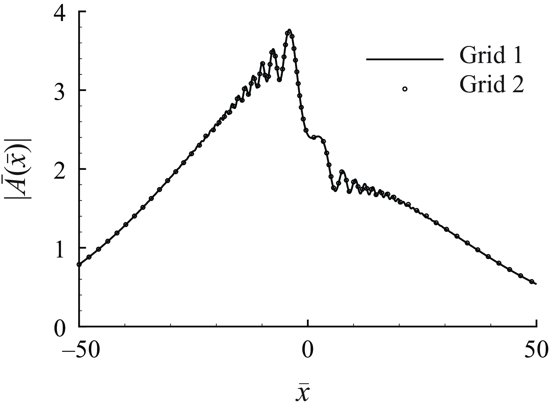
Effects of the initial amplitude $\breve {a}_0$
on the solution to the composite amplitude equation (4.8) with
$\breve {a}_0$
on the solution to the composite amplitude equation (4.8) with $Re=10^4$
,
$Re=10^4$
, $\bar {p}_I=40$
and
$\bar {p}_I=40$
and $\bar \alpha _d=0$
: (
$\bar \alpha _d=0$
: ( $a$
)
$a$
) $\breve {a}_0=1$
; (
$\breve {a}_0=1$
; ( $b$
)
$b$
) $\breve {a}_0=3$
; (
$\breve {a}_0=3$
; ( $c$
)
$c$
) $\breve {a}_0=4$
; (
$\breve {a}_0=4$
; ( $d$
)
$d$
) $\breve {a}_0=5$
. Thick solid lines, solution to (4.8); thin solid lines, solution to (4.10); dashed lines, nonlinear solution without impinging sound.
$\breve {a}_0=5$
. Thick solid lines, solution to (4.8); thin solid lines, solution to (4.10); dashed lines, nonlinear solution without impinging sound.
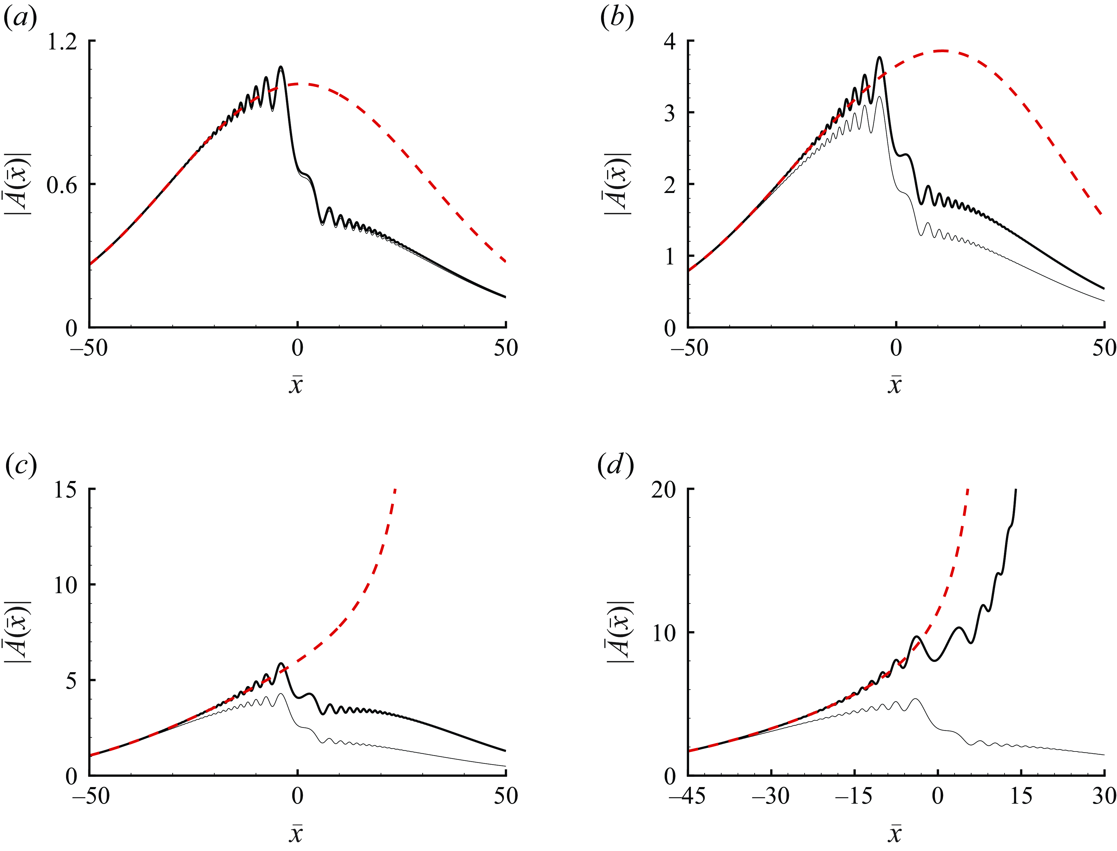
Effects of the phase of the initial amplitude, $\breve {a}_0\equiv |\breve {a}_0|{\textrm{e}}^{\textrm{i}\psi }$
, on the evolution of the radiating mode with
$\breve {a}_0\equiv |\breve {a}_0|{\textrm{e}}^{\textrm{i}\psi }$
, on the evolution of the radiating mode with $Re=10^4$
,
$Re=10^4$
, $\bar {p}_I=40$
and
$\bar {p}_I=40$
and $\bar \alpha _d=0$
for (
$\bar \alpha _d=0$
for ( $a$
)
$a$
) $|\breve {a}_0|=3$
and (
$|\breve {a}_0|=3$
and ( $b$
)
$b$
) $|\breve {a}_0|=5$
.
$|\breve {a}_0|=5$
.
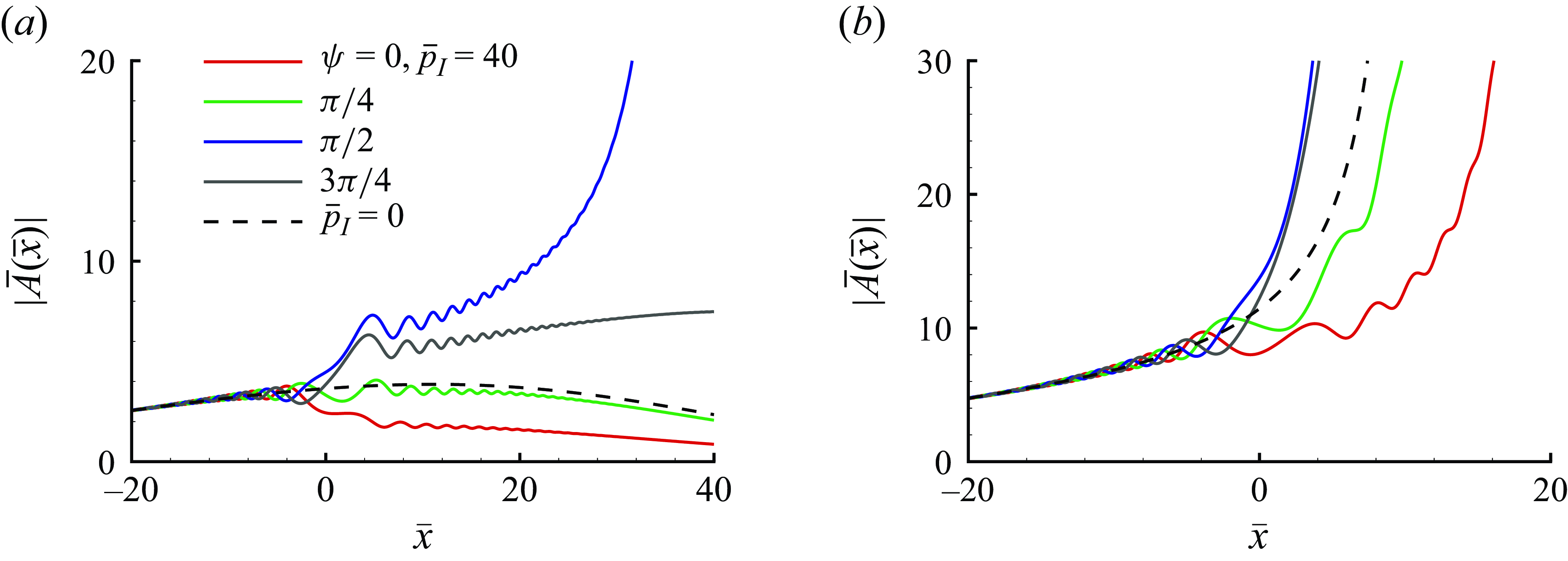
Effects of $\bar {p}_I$
on the evolution of the radiating mode with
$\bar {p}_I$
on the evolution of the radiating mode with $Re=10^4$
,
$Re=10^4$
, $\bar \alpha _d=0$
and an initial amplitude
$\bar \alpha _d=0$
and an initial amplitude $\breve {a}_0$
: (
$\breve {a}_0$
: ( $a$
)
$a$
) $\breve {a}_0=3$
and (
$\breve {a}_0=3$
and ( $b$
)
$b$
) $\breve {a}_0=5$
.
$\breve {a}_0=5$
.
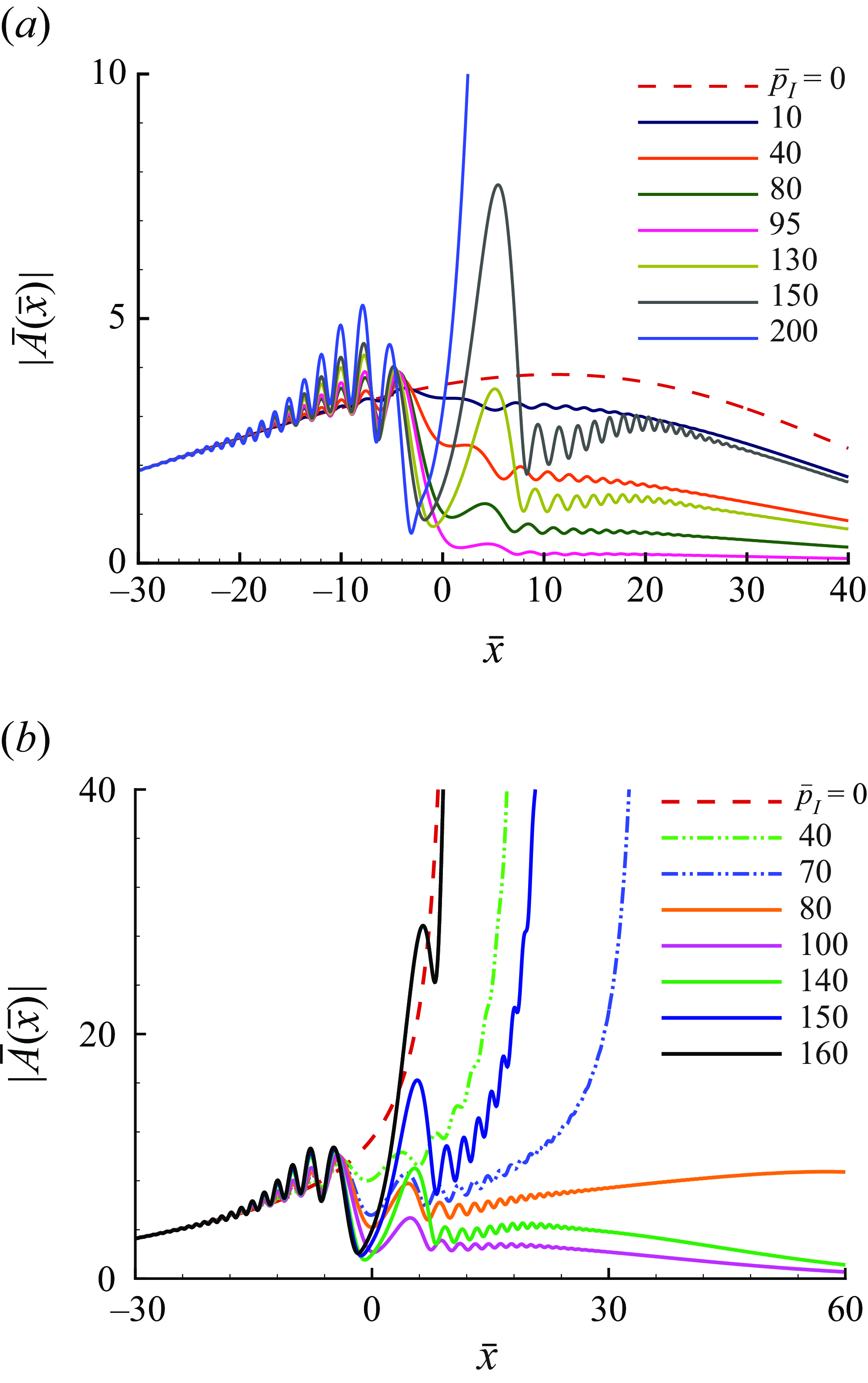
The phase of the initial amplitude also plays an important role in the evolution, and this is displayed in figure 9 for the two representative cases. The first corresponds to a small initial amplitude ( $\breve {a}_0=3$
), for which the radiating mode undergoes amplification-attenuation in the absence of the impinging sound. When the incident sound is present, the radiating mode with certain phases blows up at a finite distance, whereas the mode with other phases decays following amplification (figure 9
$\breve {a}_0=3$
), for which the radiating mode undergoes amplification-attenuation in the absence of the impinging sound. When the incident sound is present, the radiating mode with certain phases blows up at a finite distance, whereas the mode with other phases decays following amplification (figure 9 $a$
). The second case corresponds to a relatively large initial amplitude (
$a$
). The second case corresponds to a relatively large initial amplitude ( $\breve {a}_0=5$
), for which the radiating mode develops a finite-distance singularity when the incident sound is absent. In the presence of the impinging sound with a fixed intensity, the singularity remains, but altering the phase shifts the location of the singularity downstream or upstream (figure 9
$\breve {a}_0=5$
), for which the radiating mode develops a finite-distance singularity when the incident sound is absent. In the presence of the impinging sound with a fixed intensity, the singularity remains, but altering the phase shifts the location of the singularity downstream or upstream (figure 9 $b$
). In both cases, changing the phase may make the impinging sound wave to play a stabilising or destabilising role. These behaviours may have important implications for artificial control of modal growth by manipulating phase relation between the instability mode and sound wave (cf. Goldstein & Lee Reference Goldstein and Lee1992).
$b$
). In both cases, changing the phase may make the impinging sound wave to play a stabilising or destabilising role. These behaviours may have important implications for artificial control of modal growth by manipulating phase relation between the instability mode and sound wave (cf. Goldstein & Lee Reference Goldstein and Lee1992).
Figure 10 shows effects of $\bar {p}_I$
on the evolution of the radiating mode. Two cases are considered, for which the mode without the impinging sound remains bounded (figure 10
$\bar {p}_I$
on the evolution of the radiating mode. Two cases are considered, for which the mode without the impinging sound remains bounded (figure 10 $a$
) and blows up (figure 10
$a$
) and blows up (figure 10 $b$
). While the amplitude upstream increases monotonically in the case of a free mode with no incident sound (see also figure 8), once the incident sound is present, the amplitude becomes oscillatory even in its earlier linear stage. Figure 10(
$b$
). While the amplitude upstream increases monotonically in the case of a free mode with no incident sound (see also figure 8), once the incident sound is present, the amplitude becomes oscillatory even in its earlier linear stage. Figure 10( $a$
) shows that impinging sound of moderate intensity inhibits the mode, whereas further increase of the sound intensity enhances the amplification of the radiating mode and may lead to blow-up. That the incident sound changes its role as its intensity is increased also features in figure 10(
$a$
) shows that impinging sound of moderate intensity inhibits the mode, whereas further increase of the sound intensity enhances the amplification of the radiating mode and may lead to blow-up. That the incident sound changes its role as its intensity is increased also features in figure 10( $b$
), where moderate sound intensities delay the formation of a finite-distance singularity, and may even cause the radiating mode to saturate even though it would blow up in the absence of sound. This stabilising effect is reversed when the intensity is sufficiently strong: the incident sound energises the mode again, and may resurrect finite-distance singularity, which shifts upstream, consistent with the behaviour observed in the non-equilibrium regime.
$b$
), where moderate sound intensities delay the formation of a finite-distance singularity, and may even cause the radiating mode to saturate even though it would blow up in the absence of sound. This stabilising effect is reversed when the intensity is sufficiently strong: the incident sound energises the mode again, and may resurrect finite-distance singularity, which shifts upstream, consistent with the behaviour observed in the non-equilibrium regime.
5. Mach wave radiation
Similar to its counterpart on a free shear layer and a circular jet (Tam & Burton Reference Tam and Burton1984a
,Reference Tam and Burton
b
), a supersonic instability mode on a boundary layer undergoing amplification-attenuation can radiate a highly directional sound wave in the form of a Mach wave beam, as was described by Wu (2005). We shall follow his asymptotic approach to determine the complete structure of the Mach wave beam, formally in the non-parallel equilibrium regime. The disturbance outside of the boundary layer, $(\tilde \rho , \tilde {u}, \tilde {v}, \tilde {p}, \tilde \theta )$
, is governed by the linearised Euler equations. Eliminating
$(\tilde \rho , \tilde {u}, \tilde {v}, \tilde {p}, \tilde \theta )$
, is governed by the linearised Euler equations. Eliminating $\tilde \rho$
,
$\tilde \rho$
, $\tilde {u}$
,
$\tilde {u}$
, $\tilde {v}$
and
$\tilde {v}$
and $\tilde \theta$
from these equations leads to the wave equation for the pressure
$\tilde \theta$
from these equations leads to the wave equation for the pressure $\tilde {p}$
,
$\tilde {p}$
,
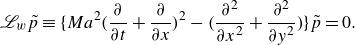 \begin{equation} \mathscr{L}_w\tilde {p}\equiv \bigg \{ Ma^2\bigg ( \frac {\partial }{\partial {t}}+\frac {\partial }{\partial {x}} \bigg )^2 -\bigg ( \frac {\partial ^2}{\partial x^2}+\frac {\partial ^2}{\partial y^2} \bigg ) \bigg \}\tilde {p}=0. \end{equation}
5.1. Near-field of the Mach wave beam
As observed by Wu (2005), the main-layer expansion (3.61) becomes disordered when $y=O(Re^{1/2})$
in view of the solution (3.14) for the pressure. The appropriate solution can be sought by introducing the variable
$y=O(Re^{1/2})$
in view of the solution (3.14) for the pressure. The appropriate solution can be sought by introducing the variable
 \begin{equation} \bar {y}=Re^{-1/2}y=O(1). \end{equation}
The perturbation in this region, referred to as the ‘near-field’ of the Mach wave beam, expands as
 \begin{equation} \tilde {p}=\bar \epsilon (p_0+Re^{-1/2}p_1+Re^{-1}p_2+\cdots ) +\bar \epsilon _s\bar {p}_I{\textrm{e}}^{\textrm{i}\alpha (x-ct+qy)}+\textrm{c.c.} \end{equation}
Substitution of this expansion into (5.1) leads to the equation for the leading-order pressure, $\mathscr{L}_w p_0=0$
. The solution may be written in the form
$\mathscr{L}_w p_0=0$
. The solution may be written in the form
 \begin{equation} p_0=\bar {p}_0(\bar {x},\bar {y}){\textrm{e}}^{\textrm{i}\alpha (x-ct-qy)}+\textrm{c.c.}, \end{equation}
where $q=\sqrt {Ma^2(1-c)^2-1}$
, and
$q=\sqrt {Ma^2(1-c)^2-1}$
, and $\bar {p}_0(\bar {x},\bar {y})$
characterises the acoustic pressure amplitude. By considering the second-order term
$\bar {p}_0(\bar {x},\bar {y})$
characterises the acoustic pressure amplitude. By considering the second-order term $p_1$
,
$p_1$
, $\bar {p}_0(\bar {x},\bar {y})$
is determined as (Wu 2005)
$\bar {p}_0(\bar {x},\bar {y})$
is determined as (Wu 2005)
 \begin{equation} \bar {p}_0(\bar {x},\bar {y})=\mathscr{C}_{\infty }\bar {A}\Big ( \bar {x}-q^{-1}[Ma^2(1-c)-1]\bar {y} \Big ), \end{equation}
which indicates that a Mach wave beam forms as a result of the amplitude modulation propagating along the characteristic lines
 \begin{equation} \bar \xi \equiv \bar {x}-q^{-1}[Ma^2(1-c)-1]\bar {y}=\mbox{constant}. \end{equation}
5.2. Far-field of the Mach wave beam
As was pointed out by Wu (2005), the expansion (5.3) and the solution (5.5) are no longer valid in the far field corresponding to the region where
 \begin{equation} \bar {y}=O(Re^{1/2}), \qquad \bar {\xi }=O(1). \end{equation}
To construct the valid solution in this far field, we introduce the variable
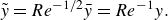 \begin{equation} \tilde {y}=Re^{-1/2}\bar {y}=Re^{-1}y. \end{equation}
The expansion for the pressure takes the form
 \begin{equation} \tilde {p}=\bar \epsilon \Big [ \tilde {p}_0(\bar {\xi },\tilde {y}) +Re^{-1}\tilde {p}_1(\bar {\xi },\tilde {y})+\cdots \Big ]{\textrm{e}}^{\textrm{i}\alpha (x-ct-qy)} +\bar \epsilon _s\bar {p}_I{\textrm{e}}^{\textrm{i}\alpha (x-ct+qy)}+\textrm{c.c.} \end{equation}
Again, the leading-order term satisfies the wave equation for an arbitrary $\tilde {p}_0$
, but the secular condition for
$\tilde {p}_0$
, but the secular condition for $\tilde {p}_1$
leads to an equation for
$\tilde {p}_1$
leads to an equation for $\tilde {p}_0$
, which is solved, subject to a matching condition with the near-field solution (5.5), to give (Wu 2005)
$\tilde {p}_0$
, which is solved, subject to a matching condition with the near-field solution (5.5), to give (Wu 2005)
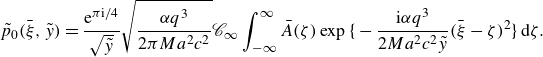 \begin{equation} \tilde {p}_0(\bar {\xi },\tilde {y})=\frac {{\textrm{e}}^{\pi \textrm{i}/4}}{\sqrt {\tilde {y}}} \sqrt {\frac {\alpha q^3}{2\pi Ma^2 c^2}}\mathscr{C}_{\infty } \int _{-\infty }^{\infty } \bar {A}(\zeta )\exp \bigg \{ -\frac {\textrm{i}\alpha q^3}{2 Ma^2 c^2\tilde {y}}(\bar {\xi }-\zeta )^2 \bigg \}\,\textrm {d}\zeta . \end{equation}
For a linear free mode, $\bar {A}(\bar {x})=\bar {a}_0{\textrm{e}}^{\sigma \bar {x}^2/2}$
, and the solution has the explicit expression
$\bar {A}(\bar {x})=\bar {a}_0{\textrm{e}}^{\sigma \bar {x}^2/2}$
, and the solution has the explicit expression
 \begin{equation} |\tilde {p}_0(\bar {\xi },\tilde {y})|= \bigg \rvert 1+\frac {\textrm{i} Ma^2 c^2\sigma }{\alpha q^3}\tilde {y} \bigg \rvert ^{-1/2} \bigg \rvert \mathscr{C}_{\infty }\bar {a}_0\exp \bigg \{ \frac {1}{2}\sigma \bar {\xi }^2 \bigg /\bigg ( 1+\frac {\textrm{i} Ma^2 c^2\sigma }{\alpha q^3}\tilde {y} \bigg ) \bigg \} \bigg \rvert . \end{equation}
5.3. Numerical evaluation
To evaluate the sound field, we rewrite the far-field pressure (5.10) as
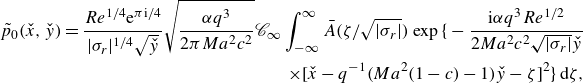 \begin{align} \tilde {p}_0(\check {x},\check {y})=\frac {Re^{1/4}{\textrm{e}}^{\pi \textrm{i}/4}}{|\sigma _r|^{1/4}\sqrt {\check {y}}} \sqrt {\frac {\alpha q^3}{2\pi Ma^2 c^2}}\mathscr{C}_{\infty } \int _{-\infty }^{\infty } \bar {A}(\zeta /\sqrt {|\sigma _r|})\exp \bigg \{ -\frac {\textrm{i}\alpha q^3 Re^{1/2}}{2 Ma^2 c^2\sqrt {|\sigma _r|}\check {y}}\nonumber \\ \times [\check {x}-q^{-1}(Ma^2(1-c)-1)\check {y}-\zeta ]^2 \bigg \}\,\textrm {d}\zeta , \end{align}
where we have introduced
 \begin{equation} \check {x}=\sqrt {|\sigma _r|}\bar {x}, \qquad \check {y}=\sqrt {|\sigma _r|}\bar {y}. \end{equation}
Contours of the far-field pressure $|\tilde {p}_0|$
calculated using the solution to the composite amplitude equation (4.8) with
$|\tilde {p}_0|$
calculated using the solution to the composite amplitude equation (4.8) with $Re=10^4$
,
$Re=10^4$
, $\breve {a}_0=3$
and
$\breve {a}_0=3$
and $\bar \alpha _d=0$
for (
$\bar \alpha _d=0$
for ( $a$
)
$a$
) $\bar {p}_I=0$
, (
$\bar {p}_I=0$
, ( $c$
)
$c$
) $\bar {p}_I=10$
and (
$\bar {p}_I=10$
and ( $e$
)
$e$
) $\bar {p}_I=40$
. Panels (
$\bar {p}_I=40$
. Panels ( $b$
), (
$b$
), ( $d$
) and (
$d$
) and ( $f$
) show the far field of panels (
$f$
) show the far field of panels ( $a$
), (
$a$
), ( $c$
) and (
$c$
) and ( $e$
), respectively.
$e$
), respectively.
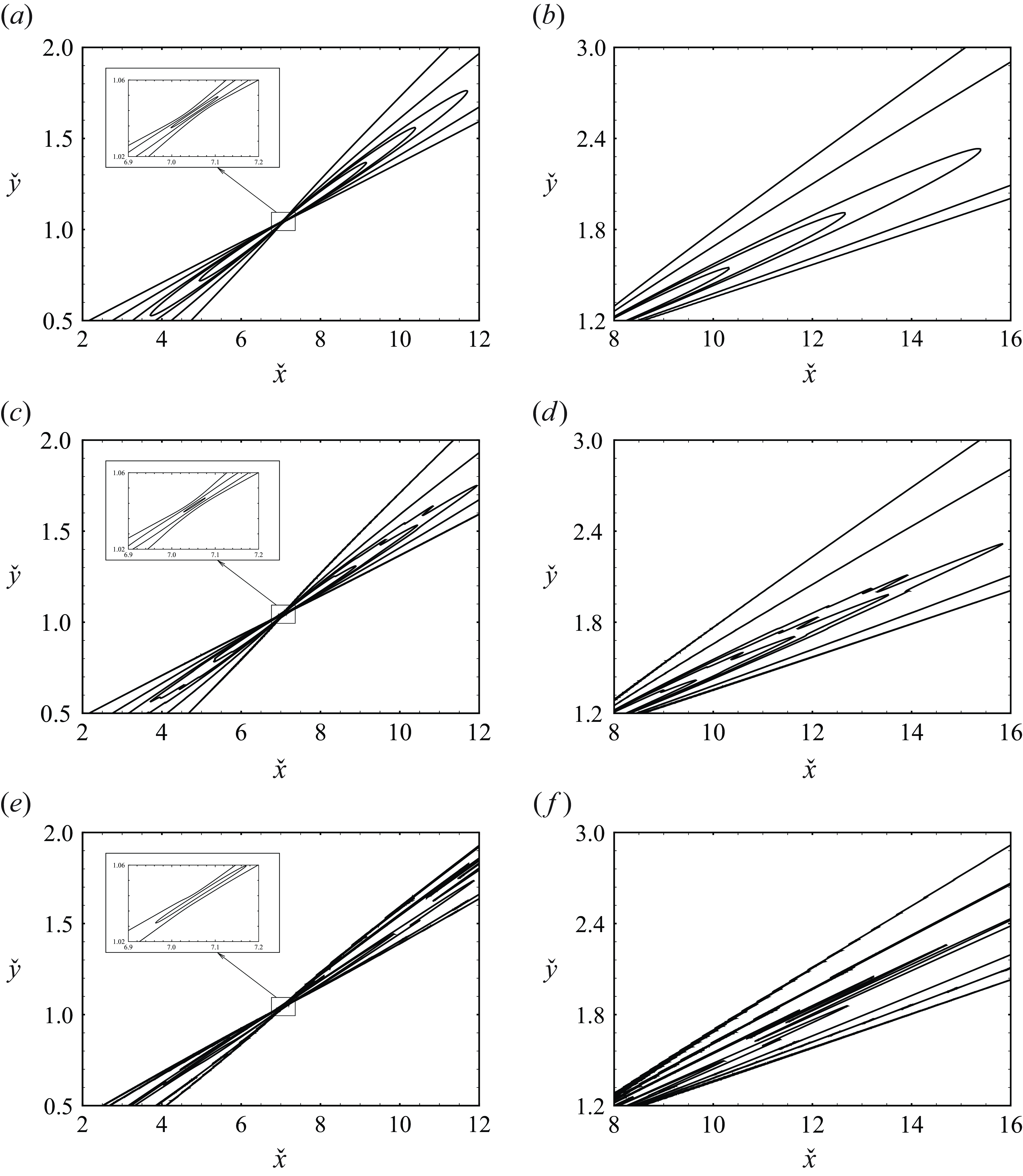
Contours of the far-field pressure $|\tilde {p}_0|$
calculated using the solution to the composite amplitude equation (4.8) with
$|\tilde {p}_0|$
calculated using the solution to the composite amplitude equation (4.8) with $Re=10^4$
,
$Re=10^4$
, $\bar {p}_I=80$
and
$\bar {p}_I=80$
and $\bar \alpha _d=0$
for (
$\bar \alpha _d=0$
for ( $a$
)
$a$
) $\breve {a}_0=3$
and (
$\breve {a}_0=3$
and ( $c$
)
$c$
) $\breve {a}_0=5$
. Panels (
$\breve {a}_0=5$
. Panels ( $b$
) and (
$b$
) and ( $d$
) show the far field of panels (
$d$
) show the far field of panels ( $a$
) and (
$a$
) and ( $c$
), respectively.
$c$
), respectively.

The acoustic field of a nonlinearly evolving mode with and without the incident sound is computed. The pressure contours predicted using the solutions to the composite amplitude equation (4.8) with $Re=10^4$
are displayed in figure 11. The pressure contours without an impinging sound are shown in figure 11(
$Re=10^4$
are displayed in figure 11. The pressure contours without an impinging sound are shown in figure 11( $a$
) with the very far field displayed in figure 11(
$a$
) with the very far field displayed in figure 11( $b$
). The emitted sound wave focuses first towards the point where the intensity attains its maximum, beyond which the contours feature a main lobe flanked by two secondary beams (Qin & Wu Reference Qin and Wu2024). The contours are rather smooth. In the presence of the incident sound with
$b$
). The emitted sound wave focuses first towards the point where the intensity attains its maximum, beyond which the contours feature a main lobe flanked by two secondary beams (Qin & Wu Reference Qin and Wu2024). The contours are rather smooth. In the presence of the incident sound with $\bar {p}_I=10$
, the smooth beam characteristic of Mach wave radiation is replaced by a rough one, featuring several spikes (figure 11
$\bar {p}_I=10$
, the smooth beam characteristic of Mach wave radiation is replaced by a rough one, featuring several spikes (figure 11 $c,d$
). Figure 11(
$c,d$
). Figure 11( $e$
) shows the sound field when the impinging sound intensity is increased to
$e$
) shows the sound field when the impinging sound intensity is increased to $\bar {p}_I=40$
. The contours become more spiky and irregular, presumably due to amplitude oscillations caused by the interaction with the sound. The structure in the far field is illustrated in figure 11(
$\bar {p}_I=40$
. The contours become more spiky and irregular, presumably due to amplitude oscillations caused by the interaction with the sound. The structure in the far field is illustrated in figure 11( $f$
).
$f$
).
Effects of the radiating mode initial amplitude on the acoustic field are studied. Contours of the far-field pressure for the case of $\breve {a}_0=3$
are depicted in figure 12(
$\breve {a}_0=3$
are depicted in figure 12( $a$
). The far-field region in figure 12(
$a$
). The far-field region in figure 12( $b$
) shows that multiple spikes are again present as a result of amplitude oscillations. Figure 12(
$b$
) shows that multiple spikes are again present as a result of amplitude oscillations. Figure 12( $c$
) shows pressure contours for the case of
$c$
) shows pressure contours for the case of $\breve {a}_0=5$
with the far field in figure 12(
$\breve {a}_0=5$
with the far field in figure 12( $d$
). The contours appear to have more sharp spikes compared with the case of
$d$
). The contours appear to have more sharp spikes compared with the case of $\breve {a}_0=3$
. In summary, the pattern of the Mach wave field is radically changed in the presence of the impinging sound, and at a fixed intensity of the incident sound, the alteration becomes more enhanced as the amplitude of the radiating mode is increased. However, the main orientation of the Mach wave beam remains little changed, which is expected since our analysis shows that the far-field distribution is a continuation of the near-field distribution, which forms as a result of the amplitude modulation propagating along the characteristic lines. The fact that the Mach wave beam in the far field remains similar to the direction of the characteristic lines can also be deduced from the near-field formula (5.5) and the far-field formula (5.10).
$\breve {a}_0=3$
. In summary, the pattern of the Mach wave field is radically changed in the presence of the impinging sound, and at a fixed intensity of the incident sound, the alteration becomes more enhanced as the amplitude of the radiating mode is increased. However, the main orientation of the Mach wave beam remains little changed, which is expected since our analysis shows that the far-field distribution is a continuation of the near-field distribution, which forms as a result of the amplitude modulation propagating along the characteristic lines. The fact that the Mach wave beam in the far field remains similar to the direction of the characteristic lines can also be deduced from the near-field formula (5.5) and the far-field formula (5.10).
6. Summary and conclusions
In this paper, the impact of an impinging sound wave on the radiating mode in a supersonic boundary layer is investigated theoretically in the limit of asymptotically large Reynolds number. The characteristic wavelength of the sound wave is taken to be comparable with the boundary-layer thickness. We consider the scenario in which the acoustic waves are the superharmonics of the radiating mode. In this case, the sound wave influences the evolution of the radiating mode through subharmonic parametric resonance or Bragg scattering mechanism. The threshold amplitude for the impinging sound wave to affect the radiating mode is obtained, and the physical processes are then described in the framework of nonlinear critical-layer theory.
The ensuing boundary-layer response, which is essentially inviscid, is considered, and the key quadratic interaction between it and the radiating mode within the critical layer is analysed to derive the amplitude equations governing the nonlinear evolution of the radiating mode in the non-equilibrium parallel and equilibrium non-parallel regimes. In the non-equilibrium regime, the growth rate of the radiating mode is modified in the upstream linear region, whilst in the nonlinear stage downstream, the amplitude of the radiating mode blows up at a finite-distance singularity, the occurrence of which is shifted upstream by the incident sound wave. Subsequently, a composite amplitude equation that takes into account both non-parallel and non-equilibrium effects is constructed, and then solved for a range of parameters to evaluate the effects of the initial amplitude and sound intensity on linear and nonlinear development of the radiating mode. The results show that for a certain range of parameters, the impinging sound wave plays a stabilising role in the evolution of the mode. An impinging sound wave of moderate intensity may suppress the growth of the mode, and may even eliminate the singularity which would occur in the absence of sound. When sound intensity exceeds a threshold, the stabilising trend is reversed and the incident sound wave may cause the amplitude of the mode to develop a finite-distance singularity. The most robust effect of the incident sound wave is that it renders amplification and attenuation of the radiating mode highly oscillatory. Finally, the composite amplitude equation is used to study the spontaneous Mach wave radiation of the instability mode. The incident sound alters the pattern of the Mach wave field significantly: the characteristic smooth beam in the absence of the incident sound is rendered rough and spiky, whilst the overall direction of the beam remains almost intact.
Given the fact that subharmonic parametric resonance usually plays a destabilising role, the stabilising effects of the impinging sound waves come as a surprise. This finding may have implications for laminar flow control using acoustic actuation. While most control strategies focus on linear growth of disturbances (e.g. Mughal Reference Mughal1998), the present work is perhaps most relevant to the control of disturbances in the nonlinear regime. Our results indicate that a particular type of acoustic wave is capable of suppressing the explosive growth of the instability mode in its nonlinear stage. Since transition to turbulence quickly follows the onset of nonlinearity, appropriate acoustic actuation based on the present mechanism may serve as a tool for delaying or even avoiding transition in flows of practical importance.
The present work is, to the best of our knowledge, the first investigation of an interesting and potentially important physical mechanism of subharmonic resonance. The mathematical analysis has revealed some rather striking impact of certain sound waves on the stability and acoustic characteristics of supersonic boundary layers. This is a case of theory advancing ahead of experiments and computations, which are yet to explore the present mechanism despite considerable interest and extensive research efforts in/on the effects of incident sound waves on transition. Presently, we cannot find any experimental or computation data to validate or support the theoretical predictions. We hope that our theoretical effort could promote experimental measurements and numerical simulations.
Finally, we comment on the issue arising from the blow-up behaviour exhibited by solutions to the amplitude equations when the incident sound intensity and/or initial amplitude is sufficiently high. As was pointed out by Qin & Wu (Reference Qin and Wu2024), the present weakly nonlinear theory loses validity near the blow-up point, and in the next stage, the disturbances would evolve on a short scale comparable to the boundary-layer thickness and be governed by the Euler equations (cf. Leib Reference Leib1991). Additionally, during its evolution towards the Euler stage, the primary disturbance may become susceptible to secondary instability. Both scenarios suggest a cascade into small scales, though precise consequences remain unclear. This process perhaps will have to be investigated through numerical solutions of the Euler or Navier–Stokes equations, since the presence of increasingly short length scales makes it difficult to obtain an asymptotic description (Cowley Reference Cowley, Aref and Phillips2001). Predicting the subsequent rapid evolution or onset of small-scale motions presents a significant challenge. However, it is conceivable that for moderate incident sound intensity and initial amplitude of radiating modes, the disturbance still retains the characteristics of a wavepacket. The near-field and far-field formulae, (5.5) and (5.10), remain valid and can still be used to compute the emitted sound waves in the respective regions once the disturbance envelope is extracted from numerical solutions.
Acknowledgements
F.Q. acknowledges the support of an EPSRC-IDS scholarship from the Department of Mathematics of Imperial College London. The referees are thanked for their comments and suggestions, which helped us improve the manuscript.
Declaration of interests
The authors report no conflict of interest.
Appendix A. Details related to main-layer analysis
The constants $\chi _a$
and
$\chi _a$
and $\chi _b$
in (3.7) are given by
$\chi _b$
in (3.7) are given by
 \begin{align} & \qquad\qquad\qquad\qquad\qquad\qquad \chi _{a}=-\frac {3}{4}\bigg ( \frac {\bar {T}_c^\prime }{\bar {T}_c}-\frac {\bar {U}_c^{\prime \prime }}{\bar {U}_c^\prime } \bigg ), \end{align}
 \begin{align} \chi _{b}&=\frac {\alpha ^2}{4}\bigg [ \frac {\bar {T}_c^{\prime \prime }}{\bar {T}_c}-\bigg ( \frac {\bar {T}_c^\prime }{\bar {T}_c} \bigg )^2 +\frac {1}{2}\bigg ( \frac {\bar {U}_c^{\prime \prime }}{\bar {U}_c^\prime } \bigg )^2 -\frac {2}{3}\frac {\bar {U}_c^{\prime \prime \prime }}{\bar {U}_c^\prime }-\frac {Ma^2(\bar {U}_c^\prime )^2}{\bar {T}_c} -\frac {\alpha ^2}{2}+\frac {11}{12}\bigg ( \frac {\bar {T}_c^\prime }{\bar {T}_c}-\frac {\bar {U}_c^{\prime \prime }}{\bar {U}_c^\prime } \bigg )^2 \bigg ].\end{align}
The second terms in the expansion (3.2), $(\hat {\rho }_1, \hat {u}_1, \hat {v}_1, \hat {p}_1, \hat {\theta }_1)$
, are found to be governed by the equations,
$(\hat {\rho }_1, \hat {u}_1, \hat {v}_1, \hat {p}_1, \hat {\theta }_1)$
, are found to be governed by the equations,
 \begin{align} &\textrm{i}\alpha ({\bar {U}}-c)\hat {\rho }_1+\bar {R}^\prime \hat {v}_1+\bar {R}(\textrm{i}\alpha \hat {u}_1+\hat {v}_1^\prime )=F_c, \\[-12pt] \nonumber \end{align}
 \begin{align} &\quad\textrm{i}\alpha ({\bar {U}}-c)\hat {u}_1+{\bar {U}}^\prime \hat {v}_1=-\textrm{i}\alpha {\bar {T}}\hat {p}_1+F_x, \\[-12pt] \nonumber \end{align}
 \begin{align} &\qquad\textrm{i}\alpha ({\bar {U}}-c)\hat {v}_1=-{\bar {T}}\hat {p}_1^\prime +F_y, \\[-12pt] \nonumber \end{align}
 \begin{align} &\textrm{i}\alpha ({\bar {U}}-c)\hat {\theta }_1+{\bar {T}}^\prime \hat {v}_1 =\textrm{i}\alpha (\gamma -1)Ma^2({\bar {U}}-c){\bar {T}}\hat {p}_1+F_e, \\[-12pt] \nonumber \end{align}
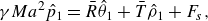 \begin{align} &\qquad\gamma Ma^2 \hat {p}_1=\bar {R}\hat {\theta }_1+{\bar {T}}\hat {\rho }_1+F_s,\end{align}
where the forcing terms, $F_c$
,
$F_c$
, $F_x$
,
$F_x$
, $F_y$
,
$F_y$
, $F_e$
and
$F_e$
and $F_s$
, are given by (Qin Reference Qin2024)
$F_s$
, are given by (Qin Reference Qin2024)
 \begin{align} & \qquad\qquad F_c=-\tilde {A}^\prime ({\bar {U}}\hat {\rho }_0+\bar {R}\hat {u}_0) -\bar {x}_1 \tilde {A}(\textrm{i}\alpha {\bar {U}}_1\hat {\rho }_0+\textrm{i}\alpha \bar {R}_1\hat {u}_0 +\bar {R}_1\hat {v}_0^\prime +\bar {R}_1^\prime \hat {v}_0), \\[-12pt] \nonumber \end{align}
 \begin{align} & F_x=-\tilde {A}^\prime ({\bar {U}}\hat {u}_0+{\bar {T}}\hat {p}_0) -\bar {x}_1 \tilde {A}[\textrm{i}\alpha {\bar {U}}_1\hat {u}_0+{\bar {U}}_1^\prime \hat {v}_0 +\textrm{i}\alpha {\bar {T}}\bar {R}_1({\bar {U}}-c)\hat {u}_0 +{\bar {T}}\bar {R}_1{\bar {U}}^\prime \hat {v}_0], \\[-12pt] \nonumber \end{align}
 \begin{align} & \qquad\qquad\qquad\qquad F_y=-\tilde {A}^\prime {\bar {U}}\hat {v}_0 -\bar {x}_1 \tilde {A}[\textrm{i}\alpha {\bar {U}}_1\hat {v}_0 +\textrm{i}\alpha {\bar {T}}\bar {R}_1({\bar {U}}-c)\hat {v}_0], \\[-12pt] \nonumber \end{align}
 \begin{align} & F_e = -\tilde {A}^\prime [{\bar {U}}\hat {\theta }_0-(\gamma -1)M^2{\bar {T}}{\bar {U}}\hat {p}_0] -\bar {x}_1 \tilde {A}[\textrm{i}\alpha {\bar {U}}_1\hat {\theta }_0+{\bar {T}}_1^\prime \hat {v}_0 +\textrm{i}\alpha {\bar {T}}\bar {R}_1({\bar {U}}-c)\hat {\theta }_0 \nonumber \\ & \qquad\qquad\qquad\qquad\qquad\qquad +{\bar {T}}\bar {R}_1{\bar {T}}^\prime \hat {v}_0 -\textrm{i}\alpha (\gamma -1)Ma^2{\bar {T}}{\bar {U}}_1\hat {p}_0], \\[-12pt] \nonumber \end{align}
 \begin{align} & \qquad\qquad\qquad\qquad\qquad\qquad F_s =\bar {x}_1 \tilde {A}(\bar {R}_1\hat {\theta }_0+{\bar {T}}_1\hat {\rho }_0),\end{align}
with $\bar {R}_1=-{\bar {T}}_1/{\bar {T}}^2$
.
$\bar {R}_1=-{\bar {T}}_1/{\bar {T}}^2$
.
The integrals $I_1$
and
$I_1$
and $I_2$
in (3.19) are given by
$I_2$
in (3.19) are given by
 \begin{align} I_1=\int _{0}^{\infty } \bigg \{ \bigg [ \frac {2\bar {U}^\prime }{{\bar {U}}-c} \bigg ( \frac {{\bar {U}}_1}{{\bar {U}}-c}-\frac {{\bar {U}}_1^\prime }{\bar {U}^\prime } \bigg )& +\frac {\bar {T}^\prime }{{\bar {T}}}\bigg ( \frac {{\bar {T}}_1^\prime }{\bar {T}^\prime }-\frac {{\bar {T}}_1}{{\bar {T}}} \bigg ) \bigg ] \frac {{\bar {T}}\hat {p}_0\hat {p}_0^\prime }{({\bar {U}}-c)^2}\nonumber\\ &+\alpha ^2 Ma^2\bigg ( \frac {2{\bar {U}}_1}{{\bar {U}}-c}-\frac {{\bar {T}}_1}{{\bar {T}}} \bigg ) \hat {p}_0^2 \bigg \} \,\textrm {d} y, \end{align}
 \begin{equation} I_2=\int _{0}^{\infty }\bigg \{ \frac {{\bar {T}}\bar {U}^\prime \hat {p}_0\hat {p}_0^\prime }{({\bar {U}}-c)^4} +\frac {\alpha ^2}{c}\bigg [ \frac {Ma^2{\bar {U}}}{{\bar {U}}-c}-\frac {{\bar {T}}}{({\bar {U}}-c)^2} \bigg ]\hat {p}_0^2 \bigg \}\,\textrm {d} y. \end{equation}
Appendix B. Details of critical-layer analysis
B.1. The mean-flow distortion in the non-equilibrium regime
The nonlinear interaction of the fundamental wave generates a mean-flow distortion, $(U_M, V_M, \Theta _M)$
; see the expansion (3.24) in the main text. The solutions required for deriving the amplitude equation are found as (Qin & Wu Reference Qin and Wu2024)
$(U_M, V_M, \Theta _M)$
; see the expansion (3.24) in the main text. The solutions required for deriving the amplitude equation are found as (Qin & Wu Reference Qin and Wu2024)
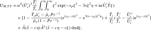 \begin{align} U_{M,YY} &= \alpha ^4(\bar {U}_c^\prime )^3\frac {\bar {T}_c^\prime }{\bar {T}_c}\int _{0}^{\infty }\!\!\!\int _{0}^{\infty } \!\xi ^2\exp (-s_p\xi ^3-3s\xi ^2\eta +\textrm{i}\alpha \bar {U}_c^\prime \bar {Y}\xi )\nonumber \\ &\quad \times \bigg [ 1-\frac {\bar {T}_c\bar {\mu }_c^\prime -\bar {\mu }_c Pr^{-1}}{\bar {\mu }_c(1-Pr^{-1})} \Big ( {\textrm{e}}^{(s_p-s)\xi ^3}-{\textrm{e}}^{3(s-s_p)\xi ^2\eta } \Big ) +\frac {\bar {T}_c}{\bar {T}_c^\prime }\bigg ( \frac {\bar {T}_c^\prime }{\bar {T}_c}-\frac {\bar {U}_c^{\prime \prime }}{\bar {U}_c^\prime } \bigg ){\textrm{e}}^{(s_p-s)\xi ^3} \bigg ]\nonumber \\ &\quad \times \tilde {A}(\tilde {x}-c\eta )\tilde {A}^*(\tilde {x}-c\eta -c\xi )\,\textrm {d}\eta \textrm {d}\xi , \end{align}
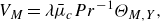 \begin{align} V_M =\lambda \bar {\mu }_c Pr^{-1}\Theta _{M,Y},\end{align}
 \begin{align} \Theta _M \!=\!\textrm{i}\alpha ^3\bar {T}_c^\prime \bar {U}_c^\prime \!\int _{0}^{\infty }\!\!\!\int _{0}^{\infty }\! \xi \exp (-s_p\xi ^3\!-\!3s_p\xi ^2\eta \!+\!\textrm{i}\alpha \bar {U}_c^\prime \bar {Y}\xi ) \tilde {A}(\tilde {x}\!-\!c\eta )\tilde {A}^*(\tilde {x}-c\eta -c\xi )\,\textrm {d}\eta \textrm {d}\xi .\end{align}
B.2. Mean-flow distortion and interaction at cubic level in the equilibrium regime
The nonlinear interaction of the radiating mode generates a mean-flow distortion, $(U_M, V_M, \Theta _M)$
; see the expansion (3.64) in the main text. The relevant solutions are found as (Qin & Wu Reference Qin and Wu2024)
$(U_M, V_M, \Theta _M)$
; see the expansion (3.64) in the main text. The relevant solutions are found as (Qin & Wu Reference Qin and Wu2024)
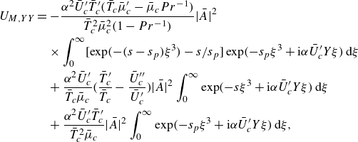 \begin{align} U_{M,YY} &= -\frac {\alpha ^2\bar {U}_c^\prime \bar {T}_c^\prime (\bar {T}_c\bar {\mu }_c^\prime -\bar {\mu }_c Pr^{-1})}{\bar {T}_c^2\bar {\mu }_c^2(1-Pr^{-1})}|\bar {A}|^2 \nonumber\\ &\quad \times \int _{0}^{\infty } [\exp (-(s-s_p)\xi ^3)-s/s_p]\exp (-s_p\xi ^3+\textrm{i}\alpha \bar {U}_c^\prime Y\xi )\,\textrm {d}\xi \nonumber\\ &\quad +\frac {\alpha ^2\bar {U}_c^\prime }{\bar {T}_c\bar {\mu }_c}\bigg ( \frac {\bar {T}_c^\prime }{\bar {T}_c}-\frac {\bar {U}_c^{\prime \prime }}{\bar {U}_c^\prime } \bigg )|\bar {A}|^2 \int _{0}^{\infty } \exp (-s\xi ^3+\textrm{i}\alpha \bar {U}_c^\prime Y\xi )\,\textrm {d}\xi \nonumber\\ &\quad +\frac {\alpha ^2\bar {U}_c^\prime \bar {T}_c^\prime }{\bar {T}_c^2\bar {\mu }_c}|\bar {A}|^2 \int _{0}^{\infty } \exp (-s_p\xi ^3+\textrm{i}\alpha \bar {U}_c^\prime Y\xi )\,\textrm {d}\xi , \\[-28pt] \nonumber \end{align}
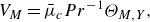 \begin{align} V_M =\bar {\mu }_c Pr^{-1}\Theta _{M,Y}, \\[-28pt] \nonumber \end{align}
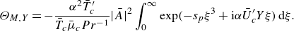 \begin{align} \Theta _{M,Y} = -\frac {\alpha ^2\bar {T}_c^\prime }{\bar {T}_c\bar {\mu }_c Pr^{-1}}|\bar {A}|^2 \int _{0}^{\infty } \exp (-s_p\xi ^3+\textrm{i}\alpha \bar {U}_c^\prime Y\xi )\,\textrm {d}\xi . \\[-1pt] \nonumber \end{align}
We now proceed to consider the fundamental regenerated by the cubic interaction, as well as by the subharmonic resonance between the acoustic component and the leading-order fundamental. The governing equations are found to be
 \begin{align} \textrm{i}\alpha \bar {U}_c^\prime Y(-\Theta _{3}/\bar {T}_c^2)\!+\!\frac {1}{\bar {T}_c}(\textrm{i}\alpha U_3\!+\!V_{3,Y}) =\frac {V_0}{\bar {T}_c^2}\Theta _{M,Y} \!+\!\frac {1}{\bar {T}_c^2}(V^*_0\Theta _{s1,Y}\!+\!V_{s0}\Theta ^*_{1,Y}){\textrm{e}}^{2\textrm{i}\bar \alpha _d\bar {x}}+\cdots ,\end{align}
 \begin{align} \bar {\mathscr{L}}_\mu U_{3}+{\bar {U}_c^\prime }V_{3} &=-\textrm{i}\alpha \bar {T}_c P_3-V_0 U_{M,Y}-\textrm{i}\alpha P_0\Theta _M+\bar {T}_c\bar {\mu }_c^\prime \bar {U}_c^\prime \Theta _{3,Y}\nonumber \\ & \quad +(-V^*_0 U_{s1,Y}-V_{s0} U^*_{1,Y}+\textrm{i}\alpha P^*_0\Theta _{s1}-2\textrm{i}\alpha P_{s0}\Theta ^*_{1}) {\textrm{e}}^{2\textrm{i}\bar \alpha _d\bar {x}}+\cdots , \end{align}
 \begin{align} \bar {\mathscr{L}}_p\Theta _3=-V_0\Theta _{M,Y}+(-V^*_0\Theta _{s1,Y}-V_{s0}\Theta ^*_{1,Y}) {\textrm{e}}^{2\textrm{i}\bar \alpha _d\bar {x}}+\cdots ,\end{align}
where the operator $\bar {\mathscr{L}}_\mu$
is the same as
$\bar {\mathscr{L}}_\mu$
is the same as $\bar {\mathscr{L}}_p$
in (3.66) with
$\bar {\mathscr{L}}_p$
in (3.66) with $Pr=1$
. Equation (B7c
) is solved first to give
$Pr=1$
. Equation (B7c
) is solved first to give
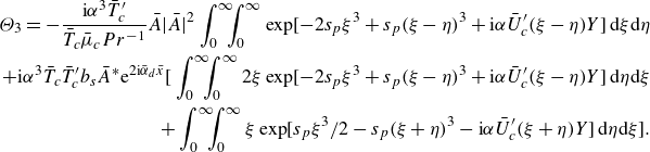 \begin{align} \Theta _3=-\frac {\textrm{i}\alpha ^3\bar {T}_c^\prime }{\bar {T}_c\bar {\mu }_c Pr^{-1}}\bar {A}|\bar {A}|^2 \int _{0}^{\infty }\!\!\!\int _{0}^{\infty } \exp [-2s_p\xi ^3+s_p(\xi -\eta )^3+\textrm{i}\alpha \bar {U}_c^\prime (\xi -\eta )Y]\,\textrm {d}\xi \textrm {d}\eta \nonumber \\ +\textrm{i}\alpha ^3\bar {T}_c\bar {T}_c^\prime b_s\bar {A}^*{\textrm{e}}^{2\textrm{i}\bar \alpha _d\bar {x}} \bigg [ \int _{0}^{\infty }\!\!\!\int _{0}^{\infty } 2\xi \exp [-2s_p\xi ^3+s_p(\xi -\eta )^3+\textrm{i}\alpha \bar {U}_c^\prime (\xi -\eta )Y]\,\textrm {d}\eta \textrm {d}\xi\nonumber \\ +\int _{0}^{\infty }\!\!\!\int _{0}^{\infty } \xi \exp [s_p\xi ^3/2-s_p(\xi +\eta )^3-\textrm{i}\alpha \bar {U}_c^\prime (\xi +\eta )Y]\,\textrm {d}\eta \textrm {d}\xi \bigg ]. \end{align}
Equations (B7a ) and (B7b ) can be reduced to
 \begin{align} \bar {\mathscr{L}}_\mu U_{3,Y}=&-V_0 U_{M,YY}-\textrm{i}\alpha P_0\Theta _{M,Y} +\bar {U}_c^\prime (\bar {T}_c\bar {\mu }_c^\prime -\bar {\mu }_c Pr^{-1})\Theta _{3,YY}\nonumber \\ &+(-V^*_0 U_{s1,YY}-V_{s0} U^*_{1,YY}+\textrm{i}\alpha P^*_0\Theta _{s1,Y}-2\textrm{i}\alpha P_{s0}\Theta ^*_{1,Y}) {\textrm{e}}^{2\textrm{i}\bar \alpha _d\bar {x}}+\cdots . \end{align}
Again solve (B9) by Fourier transform, and matching $U_3$
with the outer solution (3.18) determines the jump
$U_3$
with the outer solution (3.18) determines the jump
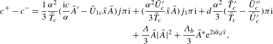 \begin{align} c^{+}-c^{-}=\frac {1}{3}\frac {\alpha ^2}{\bar {T}_c} \bigg ( \frac {\textrm{i} c}{\alpha }\bar {A}^\prime -{\bar {U}}_{1c}\bar {x} \bar {A} \bigg )j\pi \textrm{i} &+\bigg ( \frac {\alpha ^2\bar {U}_c^\prime }{3\bar {T}_c}\bar {x} \bar {A} \bigg )j_1\pi \textrm{i} +d\frac {\alpha ^2}{3}\bigg ( \frac {\bar {T}_c^\prime }{\bar {T}_c}-\frac {\bar {U}_c^{\prime \prime }}{\bar {U}_c^\prime } \bigg )\pi \textrm{i}\nonumber \\ & +\frac {\Lambda }{3}\bar {A}|\bar {A}|^2+\frac {\Lambda _b}{3}\bar {A}^*{\textrm{e}}^{2\textrm{i}\bar \alpha _d\bar {x}}, \end{align}
where we have put
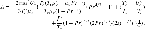 \begin{align} \Lambda =-\frac {2\pi \textrm{i}\alpha ^4\bar {U}_c^\prime }{3\bar {T}_c^2\bar {\mu }_c}\bigg \{ \frac {\bar {T}_c^\prime (\bar {T}_c\bar {\mu }_c^\prime -\bar {\mu }_c Pr^{-1})}{\bar {T}_c\bar {\mu }_c(1-Pr^{-1})} (Pr^{4/3}-1) +\bigg ( \frac {\bar {T}_c^\prime }{\bar {T}_c}-\frac {\bar {U}_c^{\prime \prime }}{\bar {U}_c^\prime } \bigg )\nonumber \\ +\frac {\bar {T}_c^\prime }{\bar {T}_c}(1+Pr)^{2/3}(2Pr)^{1/3} \bigg \}(2s)^{-1/3}\Gamma ({\textstyle \frac {1}{3}}), \end{align}
 \begin{align} \Lambda _b=\frac {4\pi \textrm{i}\alpha ^4\bar {U}_c^\prime \bar {b}_s}{3}\bigg \{ \frac {\bar {T}_c^\prime (\bar {T}_c\bar {\mu }_c^\prime -\bar {\mu }_c Pr^{-1})}{\bar {T}_c\bar {\mu }_c(1-Pr^{-1})} (Pr^{2/3}-1) +\bigg ( \frac {\bar {T}_c^\prime }{\bar {T}_c}-\frac {\bar {U}_c^{\prime \prime }}{\bar {U}_c^\prime } \bigg )\nonumber \\ +\frac {\bar {T}_c^\prime }{\bar {T}_c}(1+Pr)^{-2/3}(2Pr)^{2/3} \bigg \}(2s)^{-2/3}\Gamma ({\textstyle \frac {2}{3}}), \end{align}
with $\bar {b}_s=\bar {b}_s(\bar {p}_I)$
being given by (3.32) and
$\bar {b}_s=\bar {b}_s(\bar {p}_I)$
being given by (3.32) and $\Gamma$
denoting the gamma function.
$\Gamma$
denoting the gamma function.
Appendix C. Recovery of the equilibrium and non-equilibrium regimes from the composite theory
In this appendix, we show that the amplitude equations in the equilibrium and non-equilibrium regimes can be recovered from the composite amplitude equation (4.8) as the appropriate limiting cases.
First, consider recovery of the equilibrium regime. Following Wu & Huerre (Reference Wu and Huerre2009), we perform the substitution $\xi \rightarrow Re^{-1/6}\xi$
and
$\xi \rightarrow Re^{-1/6}\xi$
and $\eta \rightarrow Re^{-1/6}\eta$
, and take the limit
$\eta \rightarrow Re^{-1/6}\eta$
, and take the limit $Re\gg 1$
in (4.8). The latter then reduces to (3.70).
$Re\gg 1$
in (4.8). The latter then reduces to (3.70).
We consider next the nonlinear evolution of the perturbation with the modified growth rate. The perturbation in the non-equilibrium regime satisfies the initial condition (3.58) with the modified growth rate $\kappa$
being given by (3.56), and the eigenvector
$\kappa$
being given by (3.56), and the eigenvector $(a_r, a_i)$
given in (3.57). Let
$(a_r, a_i)$
given in (3.57). Let $\bar {A}_0$
denote the corresponding perturbation under the scaling of the composite theory, that is,
$\bar {A}_0$
denote the corresponding perturbation under the scaling of the composite theory, that is, $\bar {A}_0(\bar {x})=Re^{1/12}A_0(\tilde {x})$
. On noting (4.5), the perturbation can be written as
$\bar {A}_0(\bar {x})=Re^{1/12}A_0(\tilde {x})$
. On noting (4.5), the perturbation can be written as
 \begin{equation} \bar {A}_0=2|\bar {a}_0|{\textrm{e}}^{\bar \kappa _r\bar {x}} [|\bar {a}_{0r}|\cos (\bar \kappa _i\bar {x}+\bar \theta _1+\bar \phi _0) +\textrm{i}|\bar {a}_{0i}|\cos (\bar \kappa _i\bar {x}+\bar \theta _2+\bar \phi _0)], \end{equation}
where the modified growth rate $\bar \kappa \equiv Re^{1/6}\kappa$
and the eigenvector
$\bar \kappa \equiv Re^{1/6}\kappa$
and the eigenvector $(\bar {a}_r, \bar {a}_i)$
satisfy the same equations as (3.56) and (3.57) in the non-equilibrium regime, respectively, provided that the parameter
$(\bar {a}_r, \bar {a}_i)$
satisfy the same equations as (3.56) and (3.57) in the non-equilibrium regime, respectively, provided that the parameter $\bar {x}_1$
is replaced by the variable
$\bar {x}_1$
is replaced by the variable $\bar {x}$
and the parameters
$\bar {x}$
and the parameters $\Upsilon _b$
and
$\Upsilon _b$
and $s$
are replaced by
$s$
are replaced by $\bar \Upsilon _b$
and
$\bar \Upsilon _b$
and $\bar {s}$
with
$\bar {s}$
with
 \begin{equation} \bar \Upsilon _b=\Upsilon _b Re^{1/3}, \qquad \bar {s}=sRe^{1/2}. \end{equation}
Similarly, the rescaled nonlinear evolution equation for the perturbation in the composite theory has the same form as (3.50) in the non-equilibrium regime, provided that $\bar {x}_1$
is replaced by
$\bar {x}_1$
is replaced by $\bar {x}$
,
$\bar {x}$
, $\Upsilon$
by
$\Upsilon$
by $\bar \Upsilon$
with
$\bar \Upsilon$
with $\bar \Upsilon =\Upsilon Re^{2/3}$
, and the rescaled quantities in (C2) are used.
$\bar \Upsilon =\Upsilon Re^{2/3}$
, and the rescaled quantities in (C2) are used.
To compare the solution to the composite amplitude equation (4.8) with that to (3.50), the constants $|\bar {a}_0|$
and
$|\bar {a}_0|$
and $\bar \phi _0$
are first determined by fitting
$\bar \phi _0$
are first determined by fitting $\bar {A}_0$
with the composite solution at a particular location
$\bar {A}_0$
with the composite solution at a particular location $\bar {x}=-10$
. The resulting initial condition (C1) is used to solve the rescaled version of the nonlinear evolution equation (3.50). Figure 13 shows the comparison between the two solutions, with
$\bar {x}=-10$
. The resulting initial condition (C1) is used to solve the rescaled version of the nonlinear evolution equation (3.50). Figure 13 shows the comparison between the two solutions, with $\bar {A}_0$
representing the nonlinear perturbation under the scaling of the composite theory. There is good agreement between the two solutions, indicating that the composite theory captures the characteristics of the non-equilibrium effects.
$\bar {A}_0$
representing the nonlinear perturbation under the scaling of the composite theory. There is good agreement between the two solutions, indicating that the composite theory captures the characteristics of the non-equilibrium effects.


 Open access