


1 Introduction
The problem of topological classification for dynamical systems is solvable for systems with a uniformly hyperbolic chain-recurrent set (the set of such systems coincides with the set of the Axiom A systems [Reference Smale47], which satisfy the no-cycle condition [Reference Palis38, Reference Smale48]; this includes Anosov systems, Morse–Smale systems, horseshoe maps, etc.). Hyperbolic systems are structurally stable in the sense that if two such systems are
 $C^1$
close, then they are topologically equivalent in a neighbourhood of the chain-recurrent set. Hyperbolic systems comprise an open set in the space of smooth systems, and the structural stability entails that they are described by a discrete set of invariants.
$C^1$
close, then they are topologically equivalent in a neighbourhood of the chain-recurrent set. Hyperbolic systems comprise an open set in the space of smooth systems, and the structural stability entails that they are described by a discrete set of invariants.
The major fact in the theory of dynamical systems is that the complement to the set of structurally stable systems has a non-empty interior—the regions of structural instability, and the dynamics for systems from these regions are extremely diverse and much more complicated than in the hyperbolic case. One of the simplest mechanisms of destroying the structural stability is a homoclinic tangency (for smooth diffeomorphisms, another mechanism is a heterodimensional cycle [Reference Abraham and Smale1, Reference Bonatti and Díaz14, Reference Li and Turaev33]). Homoclinic tangency is a non-transverse intersection of the stable and unstable manifolds of a hyperbolic periodic orbit. Although any given tangency between two manifolds is a fragile object, the presence of homoclinic tangencies in a system turns out to be a persistent phenomenon. By the Newhouse theorem [Reference Newhouse35, Reference Newhouse36], there exist
 $C^2$
-open regions (the Newhouse domain) in the space of dynamical systems where systems with homoclinic tangencies are dense. The pioneering works of Newhouse have since been extended to multidimensional systems in [Reference Gonchenko, Turaev and Shilnikov27, Reference Gourmelon, Li, Mints and Turaev29, Reference Palis and Viana40, Reference Romero42]. Importantly, Newhouse regions are found in the space of parameters of many popular systems of applied interest, including the Hénon map, the Chua circuit, the Lorenz and Rössler models, etc.
$C^2$
-open regions (the Newhouse domain) in the space of dynamical systems where systems with homoclinic tangencies are dense. The pioneering works of Newhouse have since been extended to multidimensional systems in [Reference Gonchenko, Turaev and Shilnikov27, Reference Gourmelon, Li, Mints and Turaev29, Reference Palis and Viana40, Reference Romero42]. Importantly, Newhouse regions are found in the space of parameters of many popular systems of applied interest, including the Hénon map, the Chua circuit, the Lorenz and Rössler models, etc.
According to [Reference Turaev53, Reference Turaev54], the main characteristic of systems from the Newhouse domain is the ultimate richness of the dynamics. In line with this thesis, we show in the present paper that there exist
 $C^2$
-open subregions of the Newhouse domain, where systems with extremely degenerate homoclinic tangencies are dense. The result implies the existence of a new type of universal dynamics that is generic for these regions.
$C^2$
-open subregions of the Newhouse domain, where systems with extremely degenerate homoclinic tangencies are dense. The result implies the existence of a new type of universal dynamics that is generic for these regions.
1.1 Highly degenerate tangencies
Let
 $W_1$
and
$W_1$
and
 $W_2$
be two smooth submanifolds of the ambient k-dimensional manifold
$W_2$
be two smooth submanifolds of the ambient k-dimensional manifold
 $\mathcal M^k$
. Assume that they have complementary dimensions
$\mathcal M^k$
. Assume that they have complementary dimensions
 $k_1$
and
$k_1$
and
 $k_2$
, respectively, that is,
$k_2$
, respectively, that is,
 $k_1+ k_2=k$
. Let
$k_1+ k_2=k$
. Let
 $W_1$
and
$W_1$
and
 $W_2$
have a tangency, that is, they intersect at some point M and their tangent spaces
$W_2$
have a tangency, that is, they intersect at some point M and their tangent spaces
 $\mathcal T_M W_1$
and
$\mathcal T_M W_1$
and
 $\mathcal T_M W_2$
at M are not transverse. The tangency between two manifolds is itself a degenerate property. We characterize the degree of the degeneracy by the corank and the order of tangency. We say that the tangency between
$\mathcal T_M W_2$
at M are not transverse. The tangency between two manifolds is itself a degenerate property. We characterize the degree of the degeneracy by the corank and the order of tangency. We say that the tangency between
 $W_1$
and
$W_1$
and
 $W_2$
is of corank c if
$W_2$
is of corank c if
 $$ \begin{align} \begin{aligned} &\dim\mathcal M^k-\dim(\mathcal T_M W_1\oplus\mathcal T_M W_2)=\dim(\mathcal T_M W_1\cap \mathcal T_M W_2)=c. \end{aligned} \end{align} $$
To make the definition of the corank of tangency clearer, we reformulate it in the coordinate form. Near the point M, we introduce the coordinates
 $x\in \mathbb R^k$
such that the manifolds
$x\in \mathbb R^k$
such that the manifolds
 $W_1$
and
$W_1$
and
 $W_2$
are given by
$W_2$
are given by
 $$ \begin{align*} \begin{aligned} &W_1: 0=F_1(x) \quad \text{and} \quad W_2: 0=F_2(x), \end{aligned} \end{align*} $$
where
 $F_1:\mathbb R^{k}\to \mathbb R^{k_2}$
and
$F_1:\mathbb R^{k}\to \mathbb R^{k_2}$
and
 $F_2:\mathbb R^{k}\to \mathbb R^{k_1}$
are smooth functions such that
$F_2:\mathbb R^{k}\to \mathbb R^{k_1}$
are smooth functions such that
 $\text {rank}({\partial F_1}/{\partial x}) |_{M}=k_2$
and
$\text {rank}({\partial F_1}/{\partial x}) |_{M}=k_2$
and
 $\text {rank}({\partial F_2}/{\partial x})|_{M}=k_1$
. Note that the tangent spaces
$\text {rank}({\partial F_2}/{\partial x})|_{M}=k_1$
. Note that the tangent spaces
 $\mathcal T_M W_1$
and
$\mathcal T_M W_1$
and
 $\mathcal T_M W_2$
are given by
$\mathcal T_M W_2$
are given by
 $$ \begin{align*} \begin{aligned} &\mathcal T_M W_1: 0=\frac{\partial F_1}{\partial x}\bigg|_{M}\cdot x \quad \text{and} \quad \mathcal T_M W_2: 0=\frac{\partial F_2}{\partial x}\bigg|_{M}\cdot x. \end{aligned} \end{align*} $$
Let A be a
 $k\times k$
matrix defined as
$k\times k$
matrix defined as
 $$ \begin{align*} \begin{aligned} &A=\begin{pmatrix} \frac{\partial F_1}{\partial x}|_{M} \\[6pt] \frac{\partial F_2}{\partial x}|_{M} \end{pmatrix}. \end{aligned} \end{align*} $$
Equation (1) entails that the tangency between the manifolds
 $W_1$
and
$W_1$
and
 $W_2$
is of corank c if and only if
$W_2$
is of corank c if and only if
 $$ \begin{align} \begin{aligned} &k-\text{rank}\,A=\text{corank}\,A=c. \end{aligned} \end{align} $$
Now, we introduce the order of tangency. Let
 $\gamma _1(t)$
and
$\gamma _1(t)$
and
 $\gamma _2(t)$
be two curves in the manifold
$\gamma _2(t)$
be two curves in the manifold
 $\mathcal M^k$
such that
$\mathcal M^k$
such that
 $\gamma _1(0)=\gamma _2(0)=M$
and the velocity vectors
$\gamma _1(0)=\gamma _2(0)=M$
and the velocity vectors
 $\dot \gamma _1(0),\dot \gamma _2(0)$
are parallel. Then, we write
$\dot \gamma _1(0),\dot \gamma _2(0)$
are parallel. Then, we write
 $\text {ord}(\gamma _1,\gamma _2)=n$
if there exist a natural number n and non-zero constants
$\text {ord}(\gamma _1,\gamma _2)=n$
if there exist a natural number n and non-zero constants
 $C_1,C_2$
such that
$C_1,C_2$
such that
 $$ \begin{align*} \begin{aligned} &C_1\le\lim\limits_{t\to 0}\frac{|\gamma_1(t)-\gamma_2(t)|}{|t|^{n+1}}\le C_2. \end{aligned} \end{align*} $$
We say that the tangency between
 $W_1$
and
$W_1$
and
 $W_2$
is of order n (see Figures 1 and 2) if
$W_2$
is of order n (see Figures 1 and 2) if
 $$ \begin{align*} \begin{aligned} &\min\limits_{v}\Big(\max\limits_{\gamma_1,\gamma_2}(\text{ord}(\gamma_1,\gamma_2))\Big)=n, \end{aligned} \end{align*} $$
where the minimum is taken over all non-zero vectors
 $v\in \mathcal T_M W_1\cap \mathcal T_M W_2$
, the maximum is taken over all pairs of smooth non-zero curves
$v\in \mathcal T_M W_1\cap \mathcal T_M W_2$
, the maximum is taken over all pairs of smooth non-zero curves
 $\gamma _1\subset W_1$
,
$\gamma _1\subset W_1$
,
 $\gamma _2\subset W_2$
such that
$\gamma _2\subset W_2$
such that
 ${\gamma _1(0)=\gamma _2(0)=M}$
, and the velocity vectors
${\gamma _1(0)=\gamma _2(0)=M}$
, and the velocity vectors
 $\dot \gamma _1(0),\dot \gamma _2(0)$
are both parallel to v. Thus, the order of tangency measures how flat the tangency is: the higher the order, the flatter the tangency (see a coordinate definition in §2.1).
$\dot \gamma _1(0),\dot \gamma _2(0)$
are both parallel to v. Thus, the order of tangency measures how flat the tangency is: the higher the order, the flatter the tangency (see a coordinate definition in §2.1).
Manifolds
 $W_1$
and
$W_1$
and
 $W_2$
have a corank-1 tangency at the point M.
$W_2$
have a corank-1 tangency at the point M.

Manifolds
 $W_1$
and
$W_1$
and
 $W_2$
have a corank-2 tangency at the point M.
$W_2$
have a corank-2 tangency at the point M.

A generic tangency is of corank 1, that is, the manifolds
 $W_1$
and
$W_1$
and
 $W_2$
are tangent along one direction only. Systems with corank-1 homoclinic tangencies have been studied extensively over the past decades and, currently, a well-developed theory exists (see references in the books [Reference Bonatti, Díaz and Viana15, Reference Gonchenko and Shilnikov25, Reference Palis and Takens39]). The central result (the Newhouse theorem) is that in the space of smooth dynamical systems, near any system with a homoclinic tangency, there exist
$W_2$
are tangent along one direction only. Systems with corank-1 homoclinic tangencies have been studied extensively over the past decades and, currently, a well-developed theory exists (see references in the books [Reference Bonatti, Díaz and Viana15, Reference Gonchenko and Shilnikov25, Reference Palis and Takens39]). The central result (the Newhouse theorem) is that in the space of smooth dynamical systems, near any system with a homoclinic tangency, there exist
 $C^2$
-open regions where systems with corank-1 homoclinic tangencies are dense. Moreover, systems with corank-1 homoclinic tangencies can fill
$C^2$
-open regions where systems with corank-1 homoclinic tangencies are dense. Moreover, systems with corank-1 homoclinic tangencies can fill
 $C^1$
-open regions (see [Reference Asaoka4, Reference Bonatti and Díaz13, Reference Li32, Reference Simon45]). Description of all other possible
$C^1$
-open regions (see [Reference Asaoka4, Reference Bonatti and Díaz13, Reference Li32, Reference Simon45]). Description of all other possible
 $C^1$
-open regions in the space of diffeomorphisms can be found in [Reference Crovisier and Pujals20, Reference Pujals and Sambarino41].
$C^1$
-open regions in the space of diffeomorphisms can be found in [Reference Crovisier and Pujals20, Reference Pujals and Sambarino41].
Systems with homoclinic tangencies of high corank (
 $c>1$
) were first studied by Barrientos and Raibekas in [Reference Barrientos and Raibekas8]. They have shown that maps with homoclinic tangencies of high corank fill open regions in the space of smooth diffeomorphisms. Other constructions of such open regions were implemented in [Reference Asaoka6, Reference Barrientos and Raibekas9, Reference Barrientos and Raibekas10]. For applications of high-corank tangencies, see [Reference Buzzi, Crovisier and Fisher18, Reference Catalan19]. Note that in the original paper on the topic [Reference Barrientos and Raibekas8], the term ‘codimension’ is introduced instead of ‘corank’. We adhere to the standard for the singularity theory term ‘corank’ (see [Reference Arnold, Gusein-Zade and Varchenko3] and equation (2)) for two reasons. First, corank-c homoclinic tangency itself is a bifurcation not of codimension c, but of codimension
$c>1$
) were first studied by Barrientos and Raibekas in [Reference Barrientos and Raibekas8]. They have shown that maps with homoclinic tangencies of high corank fill open regions in the space of smooth diffeomorphisms. Other constructions of such open regions were implemented in [Reference Asaoka6, Reference Barrientos and Raibekas9, Reference Barrientos and Raibekas10]. For applications of high-corank tangencies, see [Reference Buzzi, Crovisier and Fisher18, Reference Catalan19]. Note that in the original paper on the topic [Reference Barrientos and Raibekas8], the term ‘codimension’ is introduced instead of ‘corank’. We adhere to the standard for the singularity theory term ‘corank’ (see [Reference Arnold, Gusein-Zade and Varchenko3] and equation (2)) for two reasons. First, corank-c homoclinic tangency itself is a bifurcation not of codimension c, but of codimension
 $c^2$
(see Appendix A). Second, the term ‘codimension of homoclinic tangency’ has been extensively used in the theory of corank-1 homoclinic tangencies [Reference Gonchenko, Gonchenko and Tatjer23, Reference Gonchenko, Ovsyannikov and Tatjer24, Reference Tatjer49] in a meaning very different from that of [Reference Barrientos and Raibekas8].
$c^2$
(see Appendix A). Second, the term ‘codimension of homoclinic tangency’ has been extensively used in the theory of corank-1 homoclinic tangencies [Reference Gonchenko, Gonchenko and Tatjer23, Reference Gonchenko, Ovsyannikov and Tatjer24, Reference Tatjer49] in a meaning very different from that of [Reference Barrientos and Raibekas8].
One of the most important properties of the Newhouse domain is the density of maps with corank-1 homoclinic tangencies of arbitrarily high orders [Reference Gonchenko, Turaev and Shilnikov22, Reference Gonchenko, Turaev and Shilnikov28]. More precisely, maps with infinitely many homoclinic tangencies of all orders are dense in the Newhouse domain in the space of two-dimensional
 $C^r$
maps (
$C^r$
maps (
 $r\ge 2$
; this includes
$r\ge 2$
; this includes
 $C^{\infty }$
and the space of real-analytic maps). This result has many applications, including universal dynamics for area-preserving maps [Reference Gonchenko, Turaev and Shilnikov22] and Beltrami fields [Reference Berger, Florio and Peralta-Salas12]. It is also essential for constructing maps with highly degenerate periodic orbits [Reference Gonchenko, Turaev and Shilnikov22, Reference Gonchenko, Turaev and Shilnikov28], maps with superexponential growth of the number of periodic points [Reference Kaloshin30] (other mechanisms for obtaining superexponential growth of the number of periodic points are discussed in [Reference Asaoka5, Reference Asaoka, Shinohara and Turaev7, Reference Berger11]) and such diffeomorphisms [Reference Turaev52] (cannot be topologically conjugate to any diffeomorphism of a higher regularity). In the multidimensional case, the density (in the Newhouse domain) of maps having infinitely many corank-1 homoclinic tangencies of all orders is proven in an upcoming paper [Reference Mints and Turaev34].
$C^{\infty }$
and the space of real-analytic maps). This result has many applications, including universal dynamics for area-preserving maps [Reference Gonchenko, Turaev and Shilnikov22] and Beltrami fields [Reference Berger, Florio and Peralta-Salas12]. It is also essential for constructing maps with highly degenerate periodic orbits [Reference Gonchenko, Turaev and Shilnikov22, Reference Gonchenko, Turaev and Shilnikov28], maps with superexponential growth of the number of periodic points [Reference Kaloshin30] (other mechanisms for obtaining superexponential growth of the number of periodic points are discussed in [Reference Asaoka5, Reference Asaoka, Shinohara and Turaev7, Reference Berger11]) and such diffeomorphisms [Reference Turaev52] (cannot be topologically conjugate to any diffeomorphism of a higher regularity). In the multidimensional case, the density (in the Newhouse domain) of maps having infinitely many corank-1 homoclinic tangencies of all orders is proven in an upcoming paper [Reference Mints and Turaev34].
In the present paper, we concentrate on the phenomenon of high-order tangencies of corank 2. Our main result is the following theorem.
Theorem 1.1. In the space of
 $C^r$
maps
$C^r$
maps
 $(r=2,\ldots ,\infty ,\omega )$
of each k-dimensional manifold with
$(r=2,\ldots ,\infty ,\omega )$
of each k-dimensional manifold with
 $k\ge 4$
, there exist open regions where maps with infinitely many orbits of corank-2 homoclinic tangencies of every order form a dense subset.
$k\ge 4$
, there exist open regions where maps with infinitely many orbits of corank-2 homoclinic tangencies of every order form a dense subset.
Further, we discuss the main idea of the proof and explain the construction of open regions from Theorem 1.1.
1.1.1 Main idea
Let f be a
 $C^r$
diffeomorphism
$C^r$
diffeomorphism
 $(r=2,\ldots ,\infty ,\omega )$
of a smooth or analytic k-dimensional manifold
$(r=2,\ldots ,\infty ,\omega )$
of a smooth or analytic k-dimensional manifold
 $\mathcal M^k$
. Suppose that f has a periodic orbit
$\mathcal M^k$
. Suppose that f has a periodic orbit
 $L_f$
of period b, that is,
$L_f$
of period b, that is,
 $L_f=\{O_f,f(O_f),\ldots ,f^{b-1}(O_f)\}$
with
$L_f=\{O_f,f(O_f),\ldots ,f^{b-1}(O_f)\}$
with
 $f^b(O_f)=O_f$
and
$f^b(O_f)=O_f$
and
 $f^i(O_f)\neq O_f$
for all
$f^i(O_f)\neq O_f$
for all
 $0<i<b$
. The eigenvalues of the Jacobian matrix for the map
$0<i<b$
. The eigenvalues of the Jacobian matrix for the map
 $f^b$
calculated at the point
$f^b$
calculated at the point
 $O_f$
are called multipliers of the periodic orbit
$O_f$
are called multipliers of the periodic orbit
 $L_f$
. The orbit
$L_f$
. The orbit
 $L_f$
is called hyperbolic if none of its multipliers lie on the unit circle. Any hyperbolic periodic orbit is structurally stable in the sense that if
$L_f$
is called hyperbolic if none of its multipliers lie on the unit circle. Any hyperbolic periodic orbit is structurally stable in the sense that if
 $L_f$
is such an orbit of the map f, then any map g, which is
$L_f$
is such an orbit of the map f, then any map g, which is
 $C^r$
-close to f, has a hyperbolic periodic orbit
$C^r$
-close to f, has a hyperbolic periodic orbit
 $L_g$
that is a continuation of
$L_g$
that is a continuation of
 $L_f$
. Here and throughout the rest of the article, we measure the distance between two maps on some compact region
$L_f$
. Here and throughout the rest of the article, we measure the distance between two maps on some compact region
 $K\subset \mathcal M^k$
. We say that two
$K\subset \mathcal M^k$
. We say that two
 $C^r$
-smooth maps are
$C^r$
-smooth maps are
 $\delta $
-close if a
$\delta $
-close if a
 $C^r$
distance between them on K does not exceed
$C^r$
distance between them on K does not exceed
 $\delta $
. If
$\delta $
. If
 $r=\infty $
, we define a
$r=\infty $
, we define a
 $C^{\infty }$
distance as
$C^{\infty }$
distance as
 $\rho _{\infty }(f_1,f_2)=\sum \nolimits ^{\infty }_{r=0}({1}/{(r+1)^2})\cdot {\rho _r(f_1,f_2)}/({1+\rho _r(f_1,f_2)})$
, where
$\rho _{\infty }(f_1,f_2)=\sum \nolimits ^{\infty }_{r=0}({1}/{(r+1)^2})\cdot {\rho _r(f_1,f_2)}/({1+\rho _r(f_1,f_2)})$
, where
 $\rho _r$
is a
$\rho _r$
is a
 $C^r$
distance. If
$C^r$
distance. If
 $r=\omega $
(the real-analytic case), we fix some small complex neighbourhoods Q of K and say that two
$r=\omega $
(the real-analytic case), we fix some small complex neighbourhoods Q of K and say that two
 $C^{\omega }$
maps are
$C^{\omega }$
maps are
 $\delta $
-close if they differ on not more than
$\delta $
-close if they differ on not more than
 $\delta $
at every point of Q.
$\delta $
at every point of Q.
We will assume that the hyperbolic periodic orbit
 $L_f$
has multipliers on both sides of the unit circle. Let
$L_f$
has multipliers on both sides of the unit circle. Let
 $\unicode{x3bb} _1,\ldots ,\unicode{x3bb} _{k_s}$
,
$\unicode{x3bb} _1,\ldots ,\unicode{x3bb} _{k_s}$
,
 $\gamma _1,\ldots ,\gamma _{k_u}$
be multipliers of
$\gamma _1,\ldots ,\gamma _{k_u}$
be multipliers of
 $L_f$
ordered so that
$L_f$
ordered so that
 $|\gamma _{k_u}|\ge \cdots \ge |\gamma _1|>1>|\unicode{x3bb} _1|\ge \cdots \ge |\unicode{x3bb} _{k_s}|$
. The multipliers inside the unit circle are said to be stable and those outside the unit circle are said to be unstable. Denote
$|\gamma _{k_u}|\ge \cdots \ge |\gamma _1|>1>|\unicode{x3bb} _1|\ge \cdots \ge |\unicode{x3bb} _{k_s}|$
. The multipliers inside the unit circle are said to be stable and those outside the unit circle are said to be unstable. Denote
 $\unicode{x3bb} =|\unicode{x3bb} _1|$
,
$\unicode{x3bb} =|\unicode{x3bb} _1|$
,
 $\gamma =|\gamma _1|$
. Those multipliers which are equal in absolute value to
$\gamma =|\gamma _1|$
. Those multipliers which are equal in absolute value to
 $\unicode{x3bb} $
or
$\unicode{x3bb} $
or
 $\gamma $
are called leading, and the rest are called non-leading. For the orbit
$\gamma $
are called leading, and the rest are called non-leading. For the orbit
 $L_f$
, there exist a smooth
$L_f$
, there exist a smooth
 $k_s$
-dimensional stable manifold
$k_s$
-dimensional stable manifold
 $W^s(L_f)$
and a smooth
$W^s(L_f)$
and a smooth
 $k_u$
-dimensional unstable manifold
$k_u$
-dimensional unstable manifold
 $W^u(L_f)$
defined as
$W^u(L_f)$
defined as
 $$ \begin{align} \begin{aligned} W^s(L_f)&=\{x\in\mathcal M^k: \text{dist}(f^m(x),L_f)\to 0 \text{ as } m\to+\infty\},\\ W^u(L_f)&=\{x\in\mathcal M^k: \text{dist}(f^{-m}(x),L_f)\to 0 \text{ as } m\to+\infty\}. \end{aligned} \end{align} $$
We will call the orbit
 $L_f$
a bi-focus if its leading stable and leading unstable multipliers are complex conjugate and simple (that is, there is only one pair of leading stable and one pair of leading unstable multipliers). So,
$L_f$
a bi-focus if its leading stable and leading unstable multipliers are complex conjugate and simple (that is, there is only one pair of leading stable and one pair of leading unstable multipliers). So,
 $\unicode{x3bb} _{1,2}=\unicode{x3bb} e^{\pm i\varphi }, \gamma _{1,2}=\gamma e^{\pm i\psi }$
, where
$\unicode{x3bb} _{1,2}=\unicode{x3bb} e^{\pm i\varphi }, \gamma _{1,2}=\gamma e^{\pm i\psi }$
, where
 $\varphi ,\psi \not =0,\pi $
. This condition implies that the dimension k of the ambient manifold is at least 4.
$\varphi ,\psi \not =0,\pi $
. This condition implies that the dimension k of the ambient manifold is at least 4.
The main idea in the proof of Theorem 1.1 is an algorithm that allows one to obtain a map with an orbit of corank-2 homoclinic tangency of high order by adding a
 $C^r$
-small perturbation to a map with a given (sufficiently large) number of orbits of corank-2 homoclinic tangency of order
$C^r$
-small perturbation to a map with a given (sufficiently large) number of orbits of corank-2 homoclinic tangency of order
 $1$
(quadratic) contained between the stable and unstable manifolds of a bi-focus periodic orbit. It is an independent result that can be applied to solving other problems (see the discussion in §1.3); therefore, we formulate it as a separate theorem.
$1$
(quadratic) contained between the stable and unstable manifolds of a bi-focus periodic orbit. It is an independent result that can be applied to solving other problems (see the discussion in §1.3); therefore, we formulate it as a separate theorem.
Theorem 1.2. Let f be a
 $C^r$
map
$C^r$
map
 $(r=2,\ldots ,\infty ,\omega )$
with a bi-focus periodic orbit
$(r=2,\ldots ,\infty ,\omega )$
with a bi-focus periodic orbit
 $L_f$
whose stable and unstable manifolds contain
$L_f$
whose stable and unstable manifolds contain
 $2^{{(n-1)(n+4)}/{2}}$
different orbits
$2^{{(n-1)(n+4)}/{2}}$
different orbits
 $(n\in \mathbb N \text { and} n\le r-1)$
of corank-2 homoclinic tangency. Then, arbitrarily
$(n\in \mathbb N \text { and} n\le r-1)$
of corank-2 homoclinic tangency. Then, arbitrarily
 $C^r$
-close to f, there exists a map g with a bi-focus periodic orbit
$C^r$
-close to f, there exists a map g with a bi-focus periodic orbit
 $L_g$
whose stable and unstable manifolds contain an orbit of corank-2 homoclinic tangency of order n.
$L_g$
whose stable and unstable manifolds contain an orbit of corank-2 homoclinic tangency of order n.
1.1.2
 $ABR^{*}$
-domain
$ABR^{*}$
-domain

A compact, topologically transitive, uniformly hyperbolic and locally maximal set
 $\Omega _f$
of a smooth map f is called a basic set. Let us recall that a set
$\Omega _f$
of a smooth map f is called a basic set. Let us recall that a set
 $\Omega _f$
is called locally maximal if there exists its compact neighbourhood V (which we will call defining) such that
$\Omega _f$
is called locally maximal if there exists its compact neighbourhood V (which we will call defining) such that
 ${\Omega _f=\bigcap \nolimits _{i\in \mathbb Z} f^{-i}(V)}$
. If a basic set is just a single hyperbolic periodic orbit, then it is said to be trivial; otherwise, it is called non-trivial. Throughout this paper, all basic sets are zero-dimensional.
${\Omega _f=\bigcap \nolimits _{i\in \mathbb Z} f^{-i}(V)}$
. If a basic set is just a single hyperbolic periodic orbit, then it is said to be trivial; otherwise, it is called non-trivial. Throughout this paper, all basic sets are zero-dimensional.
Let
 $\Omega _f$
be a basic set of the map f and let
$\Omega _f$
be a basic set of the map f and let
 $p_f$
be a point in
$p_f$
be a point in
 $\Omega _f$
. Define stable
$\Omega _f$
. Define stable
 $W^s(p_f)$
and unstable
$W^s(p_f)$
and unstable
 $W^u(p_f)$
manifolds of the point
$W^u(p_f)$
manifolds of the point
 $p_f$
as
$p_f$
as
 $$ \begin{align*} \begin{aligned} W^s(p_f)&=\{x\in\mathcal M^k: \text{dist}(f^m(x),f^m(p_f))\to 0 \text{ as } m\to+\infty\},\\ W^u(p_f)&=\{x\in\mathcal M^k: \text{dist}(f^{-m}(x),f^{-m}(p_f))\to 0 \text{ as } m\to+\infty\}. \end{aligned} \end{align*} $$
The topological dimension of the stable and unstable manifolds is the same for all points of the basic set
 $\Omega _f$
; therefore, one can define the type
$\Omega _f$
; therefore, one can define the type
 $(k_s,k_u)$
of
$(k_s,k_u)$
of
 $\Omega _f$
, where
$\Omega _f$
, where
 $k_s$
and
$k_s$
and
 $k_u$
are the dimensions of the stable and unstable manifolds, respectively. The manifolds
$k_u$
are the dimensions of the stable and unstable manifolds, respectively. The manifolds
 $W^s(p_f)$
and
$W^s(p_f)$
and
 $W^u(p_f)$
are injective
$W^u(p_f)$
are injective
 $C^r$
-immersions of
$C^r$
-immersions of
 $\mathbb R^{k_s}$
and
$\mathbb R^{k_s}$
and
 $\mathbb R^{k_u}$
, respectively, and they depend continuously on the point
$\mathbb R^{k_u}$
, respectively, and they depend continuously on the point
 $p_f$
and on the map f.
$p_f$
and on the map f.
In the same way as this is done for a hyperbolic periodic orbit (which is a trivial basic set; see equation (3)), one can introduce stable
 $W^s(\Omega _f)$
and unstable
$W^s(\Omega _f)$
and unstable
 $W^u(\Omega _f)$
manifolds of an arbitrary basic set
$W^u(\Omega _f)$
manifolds of an arbitrary basic set
 $\Omega _f$
as
$\Omega _f$
as
 $$ \begin{align*} \begin{aligned} W^s(\Omega_f)&=\{x\in\mathcal M^k: \text{dist}(f^m(x),\Omega_f)\to 0 \text{ as } m\to+\infty\},\\ W^u(\Omega_f)&=\{x\in\mathcal M^k: \text{dist}(f^{-m}(x),\Omega_f)\to 0 \text{ as } m\to+\infty\}. \end{aligned} \end{align*} $$
Let us note that
 $$ \begin{align*} \begin{aligned} &W^s(\Omega_f)=\bigcup\limits_{p_f\in\Omega_f} W^s(p_f) \quad \text{and} \quad W^u(\Omega_f)=\bigcup\limits_{p_f\in\Omega_f} W^u(p_f). \end{aligned} \end{align*} $$
According to [Reference Bowen16, Reference Smale47], the sets
 $W^s(L_f)\cap \Omega _f$
and
$W^s(L_f)\cap \Omega _f$
and
 $W^u(L_f)\cap \Omega _f$
are dense in the basic set
$W^u(L_f)\cap \Omega _f$
are dense in the basic set
 $\Omega _f$
for any periodic orbit
$\Omega _f$
for any periodic orbit
 $L_f\in \Omega _f$
. Moreover, stable and unstable manifolds of
$L_f\in \Omega _f$
. Moreover, stable and unstable manifolds of
 $L_f$
accumulate to stable and unstable manifolds of points from
$L_f$
accumulate to stable and unstable manifolds of points from
 $\Omega _f$
in the following sense: for any point
$\Omega _f$
in the following sense: for any point
 $p_f\in \Omega _f$
and any compact ball
$p_f\in \Omega _f$
and any compact ball
 $K_{p_f}$
in
$K_{p_f}$
in
 $W^s(p_f)$
or
$W^s(p_f)$
or
 $W^u(p_f)$
, there exists a compact ball
$W^u(p_f)$
, there exists a compact ball
 $K_{L_f}$
in
$K_{L_f}$
in
 $W^s(L_f)$
, respectively in
$W^s(L_f)$
, respectively in
 $W^u(L_f)$
, such that
$W^u(L_f)$
, such that
 $K_{p_f}$
and
$K_{p_f}$
and
 $K_{L_f}$
are
$K_{L_f}$
are
 $C^r$
-close.
$C^r$
-close.
Let
 $\Omega _f=\bigcap \nolimits _{i\in \mathbb Z} f^{-i}(V)$
, where V is a defining neighbourhood of
$\Omega _f=\bigcap \nolimits _{i\in \mathbb Z} f^{-i}(V)$
, where V is a defining neighbourhood of
 $\Omega _f$
, be a non-trivial basic set of type
$\Omega _f$
, be a non-trivial basic set of type
 $(k_s,k_u)$
of the map f. It is well known that for every map g that is
$(k_s,k_u)$
of the map f. It is well known that for every map g that is
 $C^r$
-close to f, the set
$C^r$
-close to f, the set
 $\Omega _g=\bigcap \nolimits _{i\in \mathbb Z} g^{-i}(V)$
(the continuation of
$\Omega _g=\bigcap \nolimits _{i\in \mathbb Z} g^{-i}(V)$
(the continuation of
 $\Omega _f$
) is also a non-trivial basic set of type
$\Omega _f$
) is also a non-trivial basic set of type
 $(k_s,k_u)$
. We say that
$(k_s,k_u)$
. We say that
 $\Omega _f$
exhibits a
$\Omega _f$
exhibits a
 $C^r$
-robust tangency of corank c if there exists a compact set
$C^r$
-robust tangency of corank c if there exists a compact set
 $\mathcal L\subset W^s(\Omega _f)\cup W^u(\Omega _f)$
with the following property: given any compact neighbourhood U of
$\mathcal L\subset W^s(\Omega _f)\cup W^u(\Omega _f)$
with the following property: given any compact neighbourhood U of
 $\mathcal L$
, there exists a
$\mathcal L$
, there exists a
 $C^r$
neighbourhood
$C^r$
neighbourhood
 $\mathcal U$
of f such that for any map
$\mathcal U$
of f such that for any map
 $g\in \mathcal U$
, there are points
$g\in \mathcal U$
, there are points
 $p_g, q_g$
in the continuation
$p_g, q_g$
in the continuation
 $\Omega _g$
for which
$\Omega _g$
for which
 $W^s(p_g)$
and
$W^s(p_g)$
and
 $W^u(q_g)$
have an orbit of corank-c tangency completely contained in U.
$W^u(q_g)$
have an orbit of corank-c tangency completely contained in U.
As mentioned above, Barrientos and Raibekas constructed in [Reference Barrientos and Raibekas8] diffeomorphisms exhibiting
 $C^2$
-robust homoclinic tangencies of high corank that admit a strongly partially hyperbolic decomposition at the tangency point. Subsequently, in [Reference Barrientos and Raibekas10], these open sets of diffeomorphisms were constructed by a different approach in which, at the tangency point, only a weakly partially hyperbolic decomposition is admitted. In these papers, the open regions with
$C^2$
-robust homoclinic tangencies of high corank that admit a strongly partially hyperbolic decomposition at the tangency point. Subsequently, in [Reference Barrientos and Raibekas10], these open sets of diffeomorphisms were constructed by a different approach in which, at the tangency point, only a weakly partially hyperbolic decomposition is admitted. In these papers, the open regions with
 $C^2$
-robust homoclinic tangencies of corank c were obtained on k-dimensional manifolds such that
$C^2$
-robust homoclinic tangencies of corank c were obtained on k-dimensional manifolds such that
 $k\ge 2c+2$
. In [Reference Barrientos and Raibekas8], Barrientos and Raibekas asked a question if such regions exist for the case of ambient manifolds of lower dimension. The affirmative answer was given by Asaoka in [Reference Asaoka6], where a blend of Barrientos–Raibekas and Newhouse approaches was employed. Thus, the following result holds.
$k\ge 2c+2$
. In [Reference Barrientos and Raibekas8], Barrientos and Raibekas asked a question if such regions exist for the case of ambient manifolds of lower dimension. The affirmative answer was given by Asaoka in [Reference Asaoka6], where a blend of Barrientos–Raibekas and Newhouse approaches was employed. Thus, the following result holds.
Proposition 1.3. [Reference Asaoka6, Reference Barrientos and Raibekas8, Reference Barrientos and Raibekas10]
Every manifold of dimension
 $k\ge 4$
admits a map f with a non-trivial basic set
$k\ge 4$
admits a map f with a non-trivial basic set
 $\Omega _f$
exhibiting a
$\Omega _f$
exhibiting a
 $C^2$
-robust tangency of corank c, which can be chosen to be any integer
$C^2$
-robust tangency of corank c, which can be chosen to be any integer
 $0<c\le [{k}/{2}]$
.
$0<c\le [{k}/{2}]$
.
Let us emphasize that the bound on c in Proposition 1.3 is sharp since for a basic set of type
 $(k_s,k_u)$
, the stable and unstable manifolds have dimension
$(k_s,k_u)$
, the stable and unstable manifolds have dimension
 $k_s$
and respectively
$k_s$
and respectively
 $k_u$
, so the corank of their tangency satisfies:
$k_u$
, so the corank of their tangency satisfies:
 $c\le \min \{k_s,k_u\}\le ({k}/{2})$
. We suggest to call the regions in the space of
$c\le \min \{k_s,k_u\}\le ({k}/{2})$
. We suggest to call the regions in the space of
 $C^r$
maps
$C^r$
maps
 $(r=2,\ldots ,\infty ,\omega )$
where tangencies of corank
$(r=2,\ldots ,\infty ,\omega )$
where tangencies of corank
 $c>1$
are
$c>1$
are
 $C^2$
-robust the corank- c Newhouse domain or, giving credit to the works of Barrientos, Raibekas and Asaoka, the ABR-domain.
$C^2$
-robust the corank- c Newhouse domain or, giving credit to the works of Barrientos, Raibekas and Asaoka, the ABR-domain.
To prove Theorem 1.1, we use the construction from Proposition 1.3. It is important for us that new orbits of corank-c tangency between
 $W^s(\Omega _f)$
and
$W^s(\Omega _f)$
and
 $W^u(\Omega _f)$
appear in a small neighbourhood U of some compact set
$W^u(\Omega _f)$
appear in a small neighbourhood U of some compact set
 $\mathcal L\subset W^s(\Omega _f)\cup W^u(\Omega _f)$
and that the size of U is related to the size of the perturbation of the map f (see the definition above). This allows us to control the position of these orbits of tangency by choosing a perturbation of the map f.
$\mathcal L\subset W^s(\Omega _f)\cup W^u(\Omega _f)$
and that the size of U is related to the size of the perturbation of the map f (see the definition above). This allows us to control the position of these orbits of tangency by choosing a perturbation of the map f.
We consider a subdomain of the corank-2 Newhouse domain that is defined as follows. Let f be a map that has a non-trivial basic set
 $\Lambda _f$
exhibiting a
$\Lambda _f$
exhibiting a
 $C^2$
-robust tangency of corank 2. Assume (see Figure 3) that
$C^2$
-robust tangency of corank 2. Assume (see Figure 3) that
 $\Lambda _f$
is homoclinically related to a bi-focus periodic orbit
$\Lambda _f$
is homoclinically related to a bi-focus periodic orbit
 $L_f$
(recall that two basic sets
$L_f$
(recall that two basic sets
 $\Lambda ^1_f$
and
$\Lambda ^1_f$
and
 $\Lambda ^2_f$
of the map f are said to be homoclinically related if there exist points
$\Lambda ^2_f$
of the map f are said to be homoclinically related if there exist points
 $p_f\in \Lambda ^1_f$
and
$p_f\in \Lambda ^1_f$
and
 $q_f\in \Lambda ^2_f$
such that
$q_f\in \Lambda ^2_f$
such that
 $W^s(p_f)\cap W^u(q_f)\not =\varnothing $
and
$W^s(p_f)\cap W^u(q_f)\not =\varnothing $
and
 $W^u(p_f)\cap W^s(q_f)\not =\varnothing $
, and these intersections are transverse). The homoclinic relation entails [Reference Shilnikov43, Reference Smale46] that there exist non-trivial basic sets, which include
$W^u(p_f)\cap W^s(q_f)\not =\varnothing $
, and these intersections are transverse). The homoclinic relation entails [Reference Shilnikov43, Reference Smale46] that there exist non-trivial basic sets, which include
 $\Lambda _f$
,
$\Lambda _f$
,
 $L_f$
, and heteroclinic orbits connecting them. Maps with these properties obviously form open regions in the space of smooth maps. We will call such regions the
$L_f$
, and heteroclinic orbits connecting them. Maps with these properties obviously form open regions in the space of smooth maps. We will call such regions the
 $ABR^{*}$
-domain.
$ABR^{*}$
-domain.
Homoclinically related non-trivial basic set
 $\Lambda _f$
and bi-focus periodic orbit
$\Lambda _f$
and bi-focus periodic orbit
 $L_f$
:
$L_f$
:
 $W^s(p_f)$
intersects
$W^s(p_f)$
intersects
 $W^u(q_f)$
at the point
$W^u(q_f)$
at the point
 $M^1$
and
$M^1$
and
 $W^u(p_f)$
intersects
$W^u(p_f)$
intersects
 $W^s(q_f)$
at the point
$W^s(q_f)$
at the point
 $M^2$
, where
$M^2$
, where
 $p_f\in \Lambda _f$
and
$p_f\in \Lambda _f$
and
 $q_f\in L_f$
.
$q_f\in L_f$
.

Theorem 1.4. Let f be a
 $C^r$
map
$C^r$
map
 $(r=2,\ldots ,\infty ,\omega )$
from the
$(r=2,\ldots ,\infty ,\omega )$
from the
 $ABR^{*}$
-domain and let
$ABR^{*}$
-domain and let
 $\Omega _f$
be any basic set containing
$\Omega _f$
be any basic set containing
 $\Lambda _f$
and
$\Lambda _f$
and
 $L_f$
. Then, arbitrarily
$L_f$
. Then, arbitrarily
 $C^r$
-close to f, there exists a map g such that for any pair of periodic orbits
$C^r$
-close to f, there exists a map g such that for any pair of periodic orbits
 $\mathcal O_g^1,\mathcal O_g^2$
in the continuation
$\mathcal O_g^1,\mathcal O_g^2$
in the continuation
 $\Omega _g$
, the stable manifold
$\Omega _g$
, the stable manifold
 $W^s(\mathcal O^1_g)$
and the unstable manifold
$W^s(\mathcal O^1_g)$
and the unstable manifold
 $W^u(\mathcal O^2_g)$
contain infinitely many orbits of corank-2 tangency of every order.
$W^u(\mathcal O^2_g)$
contain infinitely many orbits of corank-2 tangency of every order.
The map f belongs to the
 $ABR^{*}$
-domain that is
$ABR^{*}$
-domain that is
 $C^r$
-open, so Theorem 1.4 immediately implies Theorem 1.1. Now, let us explain how we prove Theorem 1.4 and why Theorem 1.2 is the key ingredient in the construction of the map g (a detailed proof is given in §2.2). Let
$C^r$
-open, so Theorem 1.4 immediately implies Theorem 1.1. Now, let us explain how we prove Theorem 1.4 and why Theorem 1.2 is the key ingredient in the construction of the map g (a detailed proof is given in §2.2). Let
 $f\in ABR^{*}$
-domain and let
$f\in ABR^{*}$
-domain and let
 $\Lambda _f$
be its non-trivial basic set exhibiting a
$\Lambda _f$
be its non-trivial basic set exhibiting a
 $C^2$
-robust tangency of corank 2. We obtain the map g as a result of applying a countable number of successive perturbations to the map f, each of which leaves a map in the
$C^2$
-robust tangency of corank 2. We obtain the map g as a result of applying a countable number of successive perturbations to the map f, each of which leaves a map in the
 $ABR^{*}$
-domain and can be made arbitrarily
$ABR^{*}$
-domain and can be made arbitrarily
 $C^r$
-small (so the total perturbation is arbitrarily
$C^r$
-small (so the total perturbation is arbitrarily
 $C^r$
-small). Further, for simplicity and clarity of notation, we omit the dependence on a map in the subscript.
$C^r$
-small). Further, for simplicity and clarity of notation, we omit the dependence on a map in the subscript.
-
(1) The basic set
$\Lambda $
and the periodic orbit L are in the same basic set
$\Omega $
; therefore,
$W^s(L)$
and
$W^u(L)$
accumulate to the stable manifold and the unstable manifold, respectively, of every point from
$\Lambda $
. It implies that by adding a
$C^r$
-small perturbation, which splits the tangency between
$W^s(\Lambda )$
and
$W^u(\Lambda )$
, we obtain a map with an orbit of corank-2 homoclinic tangency between
$W^s(L)$
and
$W^u(L)$
. The robustness (we are in the
$ABR^{*}$
-domain) entails that, in addition to the newly created orbit of corank-2 tangency between
$W^s(L)$
and
$W^u(L)$
, we also have an orbit of corank-2 tangency between
$W^s(\Lambda )$
and
$W^u(\Lambda )$
, splitting of which produces one more orbit of corank-2 tangency between
$W^s(L)$
and
$W^u(L)$
. Repeating this procedure
${h=2^{{(n-1)(n+4)}/{2}}}$
times, where n can be any natural number, we get a map with h orbits of corank-2 homoclinic tangency between
$W^s(L)$
and
$W^u(L)$
(along with some orbit of corank-2 tangency between
$W^s(\Lambda )$
and
$W^u(\Lambda )$
). -
(2) Applying Theorem 1.2, we get a map with an orbit of corank-2 homoclinic tangency of order n between
$W^s(L)$
and
$W^u(L)$
. -
(3) Let
$\mathcal O^1$
and
$\mathcal O^2$
be any two periodic orbits in the basic set
$\Omega $
. Since L also belongs to
$\Omega $
, then invariant manifolds
$W^s(\mathcal O^1)$
and
$W^u(\mathcal O^2)$
accumulate to invariant manifolds
$W^s(L)$
and
$W^u(L)$
, respectively. Therefore, adding
$C^r$
-small perturbation to split the tangency obtained at the previous step, we get a map with an orbit of corank-2 tangency of order n between
$W^s(\mathcal O^1)$
and
$W^u(\mathcal O^2)$
. -
(4) The orbit obtained in step 3 coexists with some orbit of corank-2 tangency between
$W^s(\Lambda )$
and
$W^u(\Lambda )$
, so we can repeat steps 1–3 countably many times to obtain a map with infinitely many orbits of corank-2 tangency of every order between the stable and unstable manifolds of every pair of periodic orbits of the basic set
$\Omega $
, as claimed in Theorem 1.4.


If we exclude the real-analytic case from consideration, then the presence of high-order tangencies of corank 2 in the system enables (by adding a
 $C^r$
-small perturbation to a map with high-order tangency of corank 2) making the stable and unstable manifolds locally coincide along a two-dimensional disk.
$C^r$
-small perturbation to a map with high-order tangency of corank 2) making the stable and unstable manifolds locally coincide along a two-dimensional disk.
Theorem 1.5. Let f be a
 $C^r$
map
$C^r$
map
 $(r=2,\ldots ,\infty )$
from the
$(r=2,\ldots ,\infty )$
from the
 $ABR^{*}$
-domain, and let
$ABR^{*}$
-domain, and let
 $\Omega _f$
be any basic set containing
$\Omega _f$
be any basic set containing
 $\Lambda _f$
and
$\Lambda _f$
and
 $L_f$
. Then, arbitrarily
$L_f$
. Then, arbitrarily
 $C^r$
-close to f, there exists a map h such that in a basic set
$C^r$
-close to f, there exists a map h such that in a basic set
 $\Omega _h$
, the intersection of the stable and unstable manifolds of every pair of periodic orbits contains a two-dimensional disk.
$\Omega _h$
, the intersection of the stable and unstable manifolds of every pair of periodic orbits contains a two-dimensional disk.
A similar result for corank-1 tangencies (the coincidence of stable and unstable manifolds along a curve) is obtained in [Reference Gonchenko, Turaev and Shilnikov22, Reference Gonchenko, Turaev and Shilnikov28, Reference Kaloshin30, Reference Mints and Turaev34]. It was used in [Reference Kaloshin30] for showing the genericity of the superexponential growth of the number of periodic points and in [Reference Turaev52] for the construction of maps that cannot be topologically conjugate to any diffeomorphism of a higher smoothness.
1.2 Universal two-dimensional dynamics
Results from the previous section can be applied to the construction of maps with universal two-dimensional dynamics. By a 2-universal map, one means that its iterations approximate the dynamics of every map of a two-dimensional disk arbitrarily well. To rigorously define the concept of universal dynamics, we follow the scheme from [Reference Turaev51], which provides a description for arbitrarily long iterations of a map on arbitrarily small spatial scales.
Let
 $\mathcal M^k$
be a smooth or analytic k-dimensional
$\mathcal M^k$
be a smooth or analytic k-dimensional
 $(k\ge 2)$
manifold and let
$(k\ge 2)$
manifold and let
 ${f:\mathcal M^k\rightarrow \mathcal M^k}$
be a
${f:\mathcal M^k\rightarrow \mathcal M^k}$
be a
 $C^r$
diffeomorphism
$C^r$
diffeomorphism
 $(r=2,\ldots ,\infty ,\omega )$
. Let
$(r=2,\ldots ,\infty ,\omega )$
. Let
 $U^k$
be the closed unit ball in
$U^k$
be the closed unit ball in
 $\mathbb R^k$
,
$\mathbb R^k$
,
 $B^k\subset \mathcal M^k$
be any small closed ball and
$B^k\subset \mathcal M^k$
be any small closed ball and
 $\theta : U^k\rightarrow B^k$
be a
$\theta : U^k\rightarrow B^k$
be a
 $C^r$
diffeomorphism. Given a positive n, the map
$C^r$
diffeomorphism. Given a positive n, the map
 $f^n|_{B^k}$
is a return map if
$f^n|_{B^k}$
is a return map if
 $f^n(B^k)\cap B^k\not =\varnothing $
. One can assume that the diffeomorphism
$f^n(B^k)\cap B^k\not =\varnothing $
. One can assume that the diffeomorphism
 $\theta : U^k\rightarrow B^k$
admits a
$\theta : U^k\rightarrow B^k$
admits a
 $C^r$
-smooth extension
$C^r$
-smooth extension
 $\Theta $
onto some larger ball
$\Theta $
onto some larger ball
 $V^k\supset U^k$
such that
$V^k\supset U^k$
such that
 $f^n(B^k)\subset \Theta (V^k)$
. By construction, the return map
$f^n(B^k)\subset \Theta (V^k)$
. By construction, the return map
 $f^n|_{B^k}$
is
$f^n|_{B^k}$
is
 $C^r$
-smoothly conjugate with the map
$C^r$
-smoothly conjugate with the map
 $f_{n,\Theta }=\Theta ^{-1}\circ f^n\circ \Theta $
. Thus, one obtains a
$f_{n,\Theta }=\Theta ^{-1}\circ f^n\circ \Theta $
. Thus, one obtains a
 $C^r$
map
$C^r$
map
 $f_{n,\Theta }: U^k\rightarrow \mathbb R^k$
, which is defined by the choice of the number of iterations n and by the choice of the embedding
$f_{n,\Theta }: U^k\rightarrow \mathbb R^k$
, which is defined by the choice of the number of iterations n and by the choice of the embedding
 $\Theta $
(which also fixes the ball
$\Theta $
(which also fixes the ball
 $B^k=\Theta (U^k)$
on the manifold
$B^k=\Theta (U^k)$
on the manifold
 $\mathcal M^k$
). The maps
$\mathcal M^k$
). The maps
 $f_{n,\Theta }$
are called renormalized iterations of f. The set
$f_{n,\Theta }$
are called renormalized iterations of f. The set
 $\bigcup \nolimits _{n,\Theta } f_{n,\Theta }$
of all possible renormalized iterations is called the dynamical conjugacy class of f.
$\bigcup \nolimits _{n,\Theta } f_{n,\Theta }$
of all possible renormalized iterations is called the dynamical conjugacy class of f.
Definition 1.6. Let
 $f:\mathcal M^k\rightarrow \mathcal M^k$
be a
$f:\mathcal M^k\rightarrow \mathcal M^k$
be a
 $C^r$
diffeomorphism and let m be a natural number such that
$C^r$
diffeomorphism and let m be a natural number such that
 $1\le m< k$
. We say that f has
$1\le m< k$
. We say that f has
 $C^r$
-universal m-dimensional dynamics if the
$C^r$
-universal m-dimensional dynamics if the
 $C^r$
-closure of its dynamical conjugacy class contains all maps of the unit ball
$C^r$
-closure of its dynamical conjugacy class contains all maps of the unit ball
 $U^k$
into
$U^k$
into
 $\mathbb R^k$
of the following form:
$\mathbb R^k$
of the following form:
 $$ \begin{align*} \begin{aligned} (\overline X_1,\ldots,\overline X_{k-m})&= 0, \\ (\overline X_{k-m+1},\ldots,\overline X_k)&= \Phi (X_{k-m+1},\ldots,X_k),\\ \end{aligned} \end{align*} $$
where
 $\Phi $
is an arbitrary
$\Phi $
is an arbitrary
 $C^r$
map of the unit ball
$C^r$
map of the unit ball
 $U^m$
into
$U^m$
into
 $\mathbb R^m$
.
$\mathbb R^m$
.
According to [Reference Gonchenko, Turaev and Shilnikov22, Reference Gonchenko, Turaev and Shilnikov28, Reference Mints and Turaev34], for any k-dimensional
 $C^r$
diffeomorphism
$C^r$
diffeomorphism
 $(k\ge 2, r=2,\ldots ,\infty ,\omega )$
with an orbit of corank-1 homoclinic tangency, there exists a
$(k\ge 2, r=2,\ldots ,\infty ,\omega )$
with an orbit of corank-1 homoclinic tangency, there exists a
 $C^r$
-small perturbation that produces a map with
$C^r$
-small perturbation that produces a map with
 $C^r$
-universal one-dimensional dynamics. It entails (see [Reference Gonchenko, Turaev and Shilnikov22]) that such universal maps are residual in the Newhouse regions of k-dimensional diffeomorphisms. Let us recall that a set A is said to be residual in a certain set B if it is a countable intersection of open and dense subsets in B. In the real-analytic case
$C^r$
-universal one-dimensional dynamics. It entails (see [Reference Gonchenko, Turaev and Shilnikov22]) that such universal maps are residual in the Newhouse regions of k-dimensional diffeomorphisms. Let us recall that a set A is said to be residual in a certain set B if it is a countable intersection of open and dense subsets in B. In the real-analytic case
 $r=\omega $
, a residual set can be defined as follows: a set A is residual in a certain subset B of space of real-analytic maps if, given any map f from B and any compact subset
$r=\omega $
, a residual set can be defined as follows: a set A is residual in a certain subset B of space of real-analytic maps if, given any map f from B and any compact subset
 $K\subset \mathcal M^k$
, there exists a complex neighbourhood Q of K such that the intersection of A with some open neighbourhood X of f in space of maps holomorphic on Q is the intersection of a countable collection of open and dense subsets of X. For the
$K\subset \mathcal M^k$
, there exists a complex neighbourhood Q of K such that the intersection of A with some open neighbourhood X of f in space of maps holomorphic on Q is the intersection of a countable collection of open and dense subsets of X. For the
 $ABR^{*}$
-domain, we prove the following theorem.
$ABR^{*}$
-domain, we prove the following theorem.
Theorem 1.7. In the
 $ABR^{*}$
-domain
$ABR^{*}$
-domain
 $(r=2,\ldots ,\infty ,\omega )$
, maps having
$(r=2,\ldots ,\infty ,\omega )$
, maps having
 $C^r$
-universal two-dimensional dynamics form a residual subset.
$C^r$
-universal two-dimensional dynamics form a residual subset.
Note that maps
 $\Phi $
in Definition 1.6 do not need to be invertible. Therefore, the variety of the dynamics displayed by the 2-universal maps in the sense of this definition is greater than for the 2-universal maps that are generic in the so-called absolute Newhouse domain (see [Reference Turaev53, Reference Turaev54]). Specifically, for the universal maps constructed in [Reference Turaev53], the dynamical conjugacy class is only dense among all orientation-preserving diffeomorphisms.
$\Phi $
in Definition 1.6 do not need to be invertible. Therefore, the variety of the dynamics displayed by the 2-universal maps in the sense of this definition is greater than for the 2-universal maps that are generic in the so-called absolute Newhouse domain (see [Reference Turaev53, Reference Turaev54]). Specifically, for the universal maps constructed in [Reference Turaev53], the dynamical conjugacy class is only dense among all orientation-preserving diffeomorphisms.
The concept of universal dynamics and Theorem 1.7 can be generalized to finite-parameter families of smooth and real-analytic maps. In what follows, by a
 $C^r$
family, we mean a parametric family of diffeomorphisms that are of class
$C^r$
family, we mean a parametric family of diffeomorphisms that are of class
 $C^r$
with respect to the coordinates and the parameters. If
$C^r$
with respect to the coordinates and the parameters. If
 $r=\omega $
, then we also call it an analytic family. Let
$r=\omega $
, then we also call it an analytic family. Let
 $\mathcal P_{l,r}$
be the space of all l-parameter
$\mathcal P_{l,r}$
be the space of all l-parameter
 $C^r$
families
$C^r$
families
 $(l\in \mathbb N, r=2,\ldots ,\infty ,\omega )$
of diffeomorphisms of the manifold
$(l\in \mathbb N, r=2,\ldots ,\infty ,\omega )$
of diffeomorphisms of the manifold
 $\mathcal M^k$
. Let
$\mathcal M^k$
. Let
 $\varepsilon =(\varepsilon _1,\ldots ,\varepsilon _l)$
be a vector of parameters that is defined on some l-dimensional ball
$\varepsilon =(\varepsilon _1,\ldots ,\varepsilon _l)$
be a vector of parameters that is defined on some l-dimensional ball
 $\mathcal D^l$
. Then, any family of maps
$\mathcal D^l$
. Then, any family of maps
 $f_{\varepsilon }\in \mathcal P_{l,r}$
can be considered as a map
$f_{\varepsilon }\in \mathcal P_{l,r}$
can be considered as a map
 $\mathcal M^k\times \mathcal D^l\to \mathcal M^k\times \mathcal D^l$
that acts as
$\mathcal M^k\times \mathcal D^l\to \mathcal M^k\times \mathcal D^l$
that acts as
 $(x,\varepsilon )\mapsto (f(x,\varepsilon ),\varepsilon )$
with a
$(x,\varepsilon )\mapsto (f(x,\varepsilon ),\varepsilon )$
with a
 $C^r$
map
$C^r$
map
 $f:$
$f:$
 $\mathcal M^k\times \mathcal D^l\to \mathcal M^k$
. Making use of this, in exactly the same way as it was done for maps, one can define renormalized iterations and the dynamical conjugacy class for any family
$\mathcal M^k\times \mathcal D^l\to \mathcal M^k$
. Making use of this, in exactly the same way as it was done for maps, one can define renormalized iterations and the dynamical conjugacy class for any family
 $f_{\varepsilon }\in \mathcal P_{l,r}$
.
$f_{\varepsilon }\in \mathcal P_{l,r}$
.
Definition 1.8. Let a parametric family of maps
 $f_{\varepsilon }$
belong to
$f_{\varepsilon }$
belong to
 $\mathcal P_{l,r}$
and let m be a natural number such that
$\mathcal P_{l,r}$
and let m be a natural number such that
 $1\le m< k$
. We say that
$1\le m< k$
. We say that
 $f_{\varepsilon }$
has
$f_{\varepsilon }$
has
 $C^r$
-universal m-dimensional dynamics if the
$C^r$
-universal m-dimensional dynamics if the
 $C^r$
-closure of its dynamical conjugacy class contains all l-parameter families of maps of the unit ball
$C^r$
-closure of its dynamical conjugacy class contains all l-parameter families of maps of the unit ball
 $U^k$
into
$U^k$
into
 $\mathbb R^k$
of the following form:
$\mathbb R^k$
of the following form:
 $$ \begin{align*} \begin{aligned} (\overline X_1,\ldots,\overline X_{k-m})&= 0, \\ (\overline X_{k-m+1},\ldots,\overline X_k)&= \Phi (X_{k-m+1},\ldots,X_k,\varepsilon_1,\ldots,\varepsilon_l),\\ \end{aligned} \end{align*} $$
where
 $\Phi $
is an arbitrary
$\Phi $
is an arbitrary
 $C^r$
map of the unit ball
$C^r$
map of the unit ball
 $U^{m+l}$
into
$U^{m+l}$
into
 $\mathbb R^m$
.
$\mathbb R^m$
.
Let us denote by
 $\mathcal P_{l,r}(ABR^{*})$
the subspace of the space
$\mathcal P_{l,r}(ABR^{*})$
the subspace of the space
 $\mathcal P_{l,r}$
such that all maps of each family
$\mathcal P_{l,r}$
such that all maps of each family
 $f_{\varepsilon }\in \mathcal P_{l,r}(ABR^{*})$
belong to the
$f_{\varepsilon }\in \mathcal P_{l,r}(ABR^{*})$
belong to the
 $ABR^{*}$
-domain. Then, absolutely similarly to the proof of Theorem 1.7, one can prove the following theorem.
$ABR^{*}$
-domain. Then, absolutely similarly to the proof of Theorem 1.7, one can prove the following theorem.
Theorem 1.9. In the space
 $\mathcal P_{l,r}(ABR^{*})$
,
$\mathcal P_{l,r}(ABR^{*})$
,
 $(l\in \mathbb N, r=2,\ldots ,\infty ,\omega )$
parameteric families having
$(l\in \mathbb N, r=2,\ldots ,\infty ,\omega )$
parameteric families having
 $C^r$
-universal two-dimensional dynamics form a residual subset.
$C^r$
-universal two-dimensional dynamics form a residual subset.
1.3 Further discussion
One can characterize the Newhouse domain as an open domain in the space of
 $C^r$
-systems
$C^r$
-systems
 $(r=2,\ldots ,\infty ,\omega )$
, where each system has a non-trivial basic set that exhibits a
$(r=2,\ldots ,\infty ,\omega )$
, where each system has a non-trivial basic set that exhibits a
 $C^2$
-robust tangency of corank 1 (also called wild hyperbolic set, see [Reference Newhouse36]). If the dimension of the ambient manifold
$C^2$
-robust tangency of corank 1 (also called wild hyperbolic set, see [Reference Newhouse36]). If the dimension of the ambient manifold
 $k\ge 4$
, then we can select an open subdomain of the Newhouse domain where each system has a wild hyperbolic set containing a bi-focus periodic orbit. We will call such subdomain a bi-focus Newhouse domain.
$k\ge 4$
, then we can select an open subdomain of the Newhouse domain where each system has a wild hyperbolic set containing a bi-focus periodic orbit. We will call such subdomain a bi-focus Newhouse domain.
In the paper in preparation [Reference Mints and Turaev34], we show that a
 $C^r$
-small perturbation of a map with a bi-focus periodic orbit, whose stable and unstable manifolds contain an orbit of corank-1 homoclinic tangency, leads to the creation of a map with an infinite number of orbits of corank-2 homoclinic tangency, that is, corank-2 tangencies are persistent and turn out to be a very natural phenomenon. Combining these results with an algorithm provided by Theorem 1.2 would give the following statement.
$C^r$
-small perturbation of a map with a bi-focus periodic orbit, whose stable and unstable manifolds contain an orbit of corank-1 homoclinic tangency, leads to the creation of a map with an infinite number of orbits of corank-2 homoclinic tangency, that is, corank-2 tangencies are persistent and turn out to be a very natural phenomenon. Combining these results with an algorithm provided by Theorem 1.2 would give the following statement.
In the space of k-dimensional
 $C^r$
maps, where
$C^r$
maps, where
 $k\ge 4$
and
$k\ge 4$
and
 $r=2,\ldots ,\infty ,\omega $
, in any neighbourhood of a map such that it has a bi-focus periodic orbit whose stable and unstable manifolds are tangent, there exist bi-focus Newhouse regions in which:
$r=2,\ldots ,\infty ,\omega $
, in any neighbourhood of a map such that it has a bi-focus periodic orbit whose stable and unstable manifolds are tangent, there exist bi-focus Newhouse regions in which:
-
(1) maps with infinitely many orbits of corank-2 homoclinic tangency of every order form a dense subset;
-
(2) maps having universal two-dimensional dynamics form a residual subset.
Other directions for the research on high-order homoclinic tangencies of high corank are the following. First, to prove the results of the given paper for the whole corank-2 Newhouse domain. Second, to generalize these results to the corank-c Newhouse domain with
 $c>2$
. It is the subject of our ongoing work.
$c>2$
. It is the subject of our ongoing work.
2 High-order tangencies of corank 2
In this section, we prove Theorem 1.4 that immediately implies our main result, Theorem 1.1. We assume that Theorem 1.2 holds, the proof of which is independent and given in §3.5.
In §2.1, we make some preliminary constructions, prove Lemmas 2.7, 2.9 and Corollary 2.8. In §2.2, we prove Lemma 2.10 and Theorems 1.4 and 1.5.
2.1 Splitting of corank-2 tangencies
Let f be a k-dimensional
 $C^r$
map
$C^r$
map
 ${(r=2,\ldots ,\infty ,\omega )}$
with a basic set
${(r=2,\ldots ,\infty ,\omega )}$
with a basic set
 $\Omega _f$
of type
$\Omega _f$
of type
 $(k_s,k_u)$
. Let
$(k_s,k_u)$
. Let
 $p_f,q_f$
be two points (possibly coinciding) such that
$p_f,q_f$
be two points (possibly coinciding) such that
 $p_f,q_f\in \Omega _f$
and
$p_f,q_f\in \Omega _f$
and
 $W^s(p_f), W^u(q_f)$
contain an orbit
$W^s(p_f), W^u(q_f)$
contain an orbit
 $\Gamma $
of corank-2 tangency. Let us fix a point
$\Gamma $
of corank-2 tangency. Let us fix a point
 $M\in \Gamma $
. Then, near the point M, one can introduce coordinates
$M\in \Gamma $
. Then, near the point M, one can introduce coordinates
 $(x_1,\ldots ,x_{k_s},y_1,\ldots ,y_{k_u})$
in which
$(x_1,\ldots ,x_{k_s},y_1,\ldots ,y_{k_u})$
in which
 $W^s(p_f)$
and
$W^s(p_f)$
and
 $W^u(q_f)$
locally have the form
$W^u(q_f)$
locally have the form
 $$ \begin{align} \begin{aligned} W^s(p_f)&=\{(y_1\ldots,y_{k_u})=(0,\ldots,0)\},\\ W^u(q_f)&=\{(y_1,y_2)=g_{1}(x_1,x_2,y_3,\ldots,y_{k_u}), (x_3,\ldots,x_{k_s})\\ &\quad\hspace{6pt} =g_{2}(x_1,x_2,y_3,\ldots,y_{k_u})\}, \end{aligned} \end{align} $$
where
 $g_1$
and
$g_1$
and
 $g_2$
are
$g_2$
are
 $C^r$
functions. Define a
$C^r$
functions. Define a
 $C^r$
function G as
$C^r$
function G as
 $$ \begin{align} \begin{aligned} &G(x_1,x_2)=g_1(x_1,x_2,0,\ldots,0). \end{aligned} \end{align} $$
Remark 2.1. Note that the existence of coordinates where
 $W^s(p_f)$
and
$W^s(p_f)$
and
 $W^u(q_f)$
satisfy equation (4) follows, for example, from [Reference Newhouse, Palis and Takens37, §II.6.], where it is shown that the coordinates can be introduced such that
$W^u(q_f)$
satisfy equation (4) follows, for example, from [Reference Newhouse, Palis and Takens37, §II.6.], where it is shown that the coordinates can be introduced such that
 $$ \begin{align*} \begin{aligned} W^s(p_f)&=\{(y_1\ldots,y_{k_u})=(0,\ldots,0)\},\\ W^u(q_f)&=\{(y_1,y_2)=g(x_1,x_2), (x_3,\ldots,x_{k_s})=(0,\ldots,0)\}, \end{aligned} \end{align*} $$
with a
 $C^r$
function g such that
$C^r$
function g such that
 $g(0,0)=(0,0)$
and
$g(0,0)=(0,0)$
and
 ${\partial g}/{\partial (x_1,x_2)} |_{(0,0)}=(\begin {smallmatrix} 0& 0\\ 0 & 0 \end {smallmatrix})$
. In these coordinates, the function G of equation (5) is g.
${\partial g}/{\partial (x_1,x_2)} |_{(0,0)}=(\begin {smallmatrix} 0& 0\\ 0 & 0 \end {smallmatrix})$
. In these coordinates, the function G of equation (5) is g.
Now, we can define an order of corank-2 tangency as follows.
Definition 2.2. We say that a corank-2 tangency
 $\Gamma $
is of order
$\Gamma $
is of order
 $n\le r-1$
 $(n\in \mathbb N, r=2,\ldots ,\infty ,\omega )$
if at the point
$(n\in \mathbb N, r=2,\ldots ,\infty ,\omega )$
if at the point
 $(x_1,x_2)=(0,0)$
, one has:
$(x_1,x_2)=(0,0)$
, one has:
-
(1)
${\partial ^{i+j} G}/{\partial x^i_1\partial x^j_2}=(0,0)$
for all
$i\ge 0$
,
$j\ge 0$
such that
$i+j\le n$
; and -
(2)
${\partial ^{n+1} G}/{\partial x^i_1\partial x^j_2}\not =(0,0)$
for at least one pair
$i\ge 0$
,
$j\ge 0$
such that
$i+j=n+1$
.


We say that a corank-2 tangency
 $\Gamma $
is
$\Gamma $
is
 $C^r$
-flat if r is finite and the first condition holds for
$C^r$
-flat if r is finite and the first condition holds for
 $n=r$
, or
$n=r$
, or
 $r=\infty $
and the first condition holds for all
$r=\infty $
and the first condition holds for all
 $n\in \mathbb N$
.
$n\in \mathbb N$
.
One can check, cf. [Reference Domitrz, Mormul and Pragacz21], that Definition 2.2 is equivalent to the definition of the order of tangency given in the introduction. This implies that the order of corank-2 tangency does not depend on the choice of the coordinates near the point M, which keep
 $W^s(p_f)$
and
$W^s(p_f)$
and
 $W^u(q_f)$
in the form of equation (4), and on the choice of the point
$W^u(q_f)$
in the form of equation (4), and on the choice of the point
 $M\in \Gamma $
. Also, we stress that the definition of the order of tangency requires taking
$M\in \Gamma $
. Also, we stress that the definition of the order of tangency requires taking
 $n+1$
derivatives; hence the order of tangency cannot exceed
$n+1$
derivatives; hence the order of tangency cannot exceed
 $r-1$
.
$r-1$
.
Let
 $\varepsilon $
be a vector of parameters that runs a small ball centred at
$\varepsilon $
be a vector of parameters that runs a small ball centred at
 $\varepsilon =0$
. Further, consider a finite-parameter
$\varepsilon =0$
. Further, consider a finite-parameter
 $C^r$
family of maps
$C^r$
family of maps
 $f_{\varepsilon }$
such that
$f_{\varepsilon }$
such that
 $f_{0}=f$
. We choose coordinates in such a way that for the map
$f_{0}=f$
. We choose coordinates in such a way that for the map
 $f_{\varepsilon }$
(for all small
$f_{\varepsilon }$
(for all small
 $\varepsilon $
), the manifolds
$\varepsilon $
), the manifolds
 $W^s(p_{f_\varepsilon })$
and
$W^s(p_{f_\varepsilon })$
and
 $W^u(q_{f_\varepsilon })$
near the point M are given by
$W^u(q_{f_\varepsilon })$
near the point M are given by
 $$ \begin{align*} \begin{aligned} W^s(p_{f_\varepsilon})&=\{(y_1,\ldots,y_{k_u})=(0,\ldots,0)\},\\ W^u(q_{f_\varepsilon})&=\{(y_1,y_2)=g_{1,\varepsilon}(x_1,x_2,y_3,\ldots,y_{k_u}), (x_3,\ldots,x_{k_s})\\ &\quad\hspace{6pt}=g_{2,\varepsilon}(x_1,x_2,y_3,\ldots,y_{k_u})\}, \end{aligned} \end{align*} $$
where the functions
 $g_{1,\varepsilon }, g_{2,\varepsilon }$
are of class
$g_{1,\varepsilon }, g_{2,\varepsilon }$
are of class
 $C^r$
with respect to the coordinates and parameters, and at
$C^r$
with respect to the coordinates and parameters, and at
 $\varepsilon =0$
, the functions
$\varepsilon =0$
, the functions
 $g_{1,0}, g_{2,0}$
coincide with
$g_{1,0}, g_{2,0}$
coincide with
 $g_1, g_2$
of equation (4), respectively. Further, in a similar way as above, we introduce
$g_1, g_2$
of equation (4), respectively. Further, in a similar way as above, we introduce
 $$ \begin{align*} \begin{aligned} &G_{\varepsilon}(x_1,x_2)=g_{1,\varepsilon}(x_1,x_2,0,\ldots,0), \end{aligned} \end{align*} $$
which we call the splitting function for the orbit
 $\Gamma $
. Note that
$\Gamma $
. Note that
 $G_0=G$
of equation (5). Fix an integer
$G_0=G$
of equation (5). Fix an integer
 $\tilde n$
such that
$\tilde n$
such that
 $0\le \tilde n\le r-1$
. The function
$0\le \tilde n\le r-1$
. The function
 $G_{\varepsilon }$
can be written as
$G_{\varepsilon }$
can be written as
 $$ \begin{align*} \begin{aligned} &G_{\varepsilon}(x_1,x_2)=G(x_1,x_2)+\sum\limits_{j=0}^{\tilde n}\sum\limits_{i=0}^{j} (\eta_{1,j,i},\eta_{2,j,i}) x_1^{j-i} x_2^{i} +O(\|x\|^{\tilde n+1}), \end{aligned} \end{align*} $$
where
 $\eta _{1,j,i}$
and
$\eta _{1,j,i}$
and
 $\eta _{2,j,i}$
are smooth functions of
$\eta _{2,j,i}$
are smooth functions of
 $\varepsilon $
, which we call the splitting coefficients for the orbit
$\varepsilon $
, which we call the splitting coefficients for the orbit
 $\Gamma $
. They are small in absolute value and
$\Gamma $
. They are small in absolute value and
 $\eta _{1,j,i}(0)=0$
,
$\eta _{1,j,i}(0)=0$
,
 $\eta _{2,j,i}(0)=0$
. By
$\eta _{2,j,i}(0)=0$
. By
 $O(\|x\|^{\tilde n+1})$
, we mean some function
$O(\|x\|^{\tilde n+1})$
, we mean some function
 $\zeta _{\varepsilon }(x_1,x_2)$
 $(\zeta _{0}(x_1,x_2)=(0,0))$
with the following property: there exists a positive constant C such that for all sufficiently small
$(\zeta _{0}(x_1,x_2)=(0,0))$
with the following property: there exists a positive constant C such that for all sufficiently small
 $x_1,x_2$
, one has
$x_1,x_2$
, one has
 $\zeta _{\varepsilon }(x_1,x_2)\le C\cdot \|x\|^{\tilde n+1}$
. Denote as
$\zeta _{\varepsilon }(x_1,x_2)\le C\cdot \|x\|^{\tilde n+1}$
. Denote as
 $\overline \eta _{\tilde n}$
the vector consisting of all the splitting coefficients
$\overline \eta _{\tilde n}$
the vector consisting of all the splitting coefficients
 $\eta _{1,j,i}$
,
$\eta _{1,j,i}$
,
 $\eta _{2,j,i}$
, and let
$\eta _{2,j,i}$
, and let
 $\chi (\overline \eta _{\tilde n})=\tilde n^2+3\tilde n+2$
be the total number of components of this vector.
$\chi (\overline \eta _{\tilde n})=\tilde n^2+3\tilde n+2$
be the total number of components of this vector.
Definition 2.3. We say that the parametric family of maps
 $f_{\varepsilon }$
perturbs the orbit
$f_{\varepsilon }$
perturbs the orbit
 $\Gamma $
freely up to order
$\Gamma $
freely up to order
 $\tilde n$
if
$\tilde n$
if
 $$ \begin{align*} \text{rank }\frac{\partial\overline\eta_{\tilde n}}{\partial\varepsilon}\bigg |_{\varepsilon=0}=\chi(\overline\eta_{\tilde n}). \end{align*} $$
Remark 2.4. Formally speaking, there is no relation between the order n of tangency and the order
 $\tilde n$
of the perturbation freedom. However, for most of the paper, we consider the case
$\tilde n$
of the perturbation freedom. However, for most of the paper, we consider the case
 $\tilde n=n$
. Then, for simplicity, we say that corank-2 tangency of order n splits freely.
$\tilde n=n$
. Then, for simplicity, we say that corank-2 tangency of order n splits freely.
Now, let us generalize the above constructions for any finite number of orbits of corank-2 tangency. Let
 $p^1_f,q^1_f,\ldots ,p^h_f,q^h_f$
be points in
$p^1_f,q^1_f,\ldots ,p^h_f,q^h_f$
be points in
 $\Omega _f$
such that for each
$\Omega _f$
such that for each
 $t\in \{1,\ldots ,h\}$
, the manifolds
$t\in \{1,\ldots ,h\}$
, the manifolds
 $W^s(p^t_f), W^u(q^t_f)$
contain an orbit
$W^s(p^t_f), W^u(q^t_f)$
contain an orbit
 $\Gamma ^t$
of corank-2 tangency. As above, in each orbit
$\Gamma ^t$
of corank-2 tangency. As above, in each orbit
 $\Gamma ^t$
, we choose a point
$\Gamma ^t$
, we choose a point
 $M^t\in \Gamma ^t$
and introduce coordinates near
$M^t\in \Gamma ^t$
and introduce coordinates near
 $M^t$
in which
$M^t$
in which
 $W^s(p^t_f)$
and
$W^s(p^t_f)$
and
 $W^u(q^t_f)$
take the form
$W^u(q^t_f)$
take the form
 $$ \begin{align} \begin{aligned} W^s(p^t_f)&=\{(y_1\ldots,y_{k_u})=(0,\ldots,0)\},\\ W^u(q^t_f)&=\{(y_1,y_2)=g^t_{1}(x_1,x_2,y_3,\ldots,y_{k_u}), (x_3,\ldots,x_{k_s})\\ &\quad\hspace{6pt}=g^t_{2}(x_1,x_2,y_3,\ldots,y_{k_u})\}, \end{aligned} \end{align} $$
where
 $g^t_1$
and
$g^t_1$
and
 $g^t_2$
are
$g^t_2$
are
 $C^r$
functions. Note that for simplicity of notation, we use
$C^r$
functions. Note that for simplicity of notation, we use
 $(x_1,\ldots ,x_{k_s},y_1,\ldots ,y_{k_u})$
as the coordinates in the neighbourhood of each point
$(x_1,\ldots ,x_{k_s},y_1,\ldots ,y_{k_u})$
as the coordinates in the neighbourhood of each point
 $M^t$
.
$M^t$
.
Let
 $\varepsilon $
be a vector of parameters that runs a small ball centred at
$\varepsilon $
be a vector of parameters that runs a small ball centred at
 $\varepsilon =0$
. Consider a finite-parameter
$\varepsilon =0$
. Consider a finite-parameter
 $C^r$
family of maps
$C^r$
family of maps
 $f_{\varepsilon }$
such that
$f_{\varepsilon }$
such that
 $f_{0}=f$
. Repeating the same reasoning, for all small
$f_{0}=f$
. Repeating the same reasoning, for all small
 $\varepsilon $
, we introduce a splitting function
$\varepsilon $
, we introduce a splitting function
 $G^t_{\varepsilon }$
, which can be written as
$G^t_{\varepsilon }$
, which can be written as
 $$ \begin{align*} \begin{aligned} &G^t_{\varepsilon}(x_1,x_2)=G^t(x_1,x_2)+\sum\limits_{j=0}^{\tilde n_t}\sum\limits_{i=0}^{j} (\eta^t_{1,j,i},\eta^t_{2,j,i}) x_1^{j-i} x_2^{i} +O(\|x\|^{\tilde n_t+1}), \end{aligned} \end{align*} $$
where
 $\tilde n_1,\ldots ,\tilde n_h$
are integers such that
$\tilde n_1,\ldots ,\tilde n_h$
are integers such that
 $0\le \tilde n_t\le r-1$
, and
$0\le \tilde n_t\le r-1$
, and
 $\eta ^t_{1,j,i}$
,
$\eta ^t_{1,j,i}$
,
 $\eta ^t_{2,j,i}$
are the splitting coefficients. Again, we denote as
$\eta ^t_{2,j,i}$
are the splitting coefficients. Again, we denote as
 $\overline \eta ^t_{\tilde n_t}$
the vector that consists of all the splitting coefficients
$\overline \eta ^t_{\tilde n_t}$
the vector that consists of all the splitting coefficients
 $\eta ^t_{1,j,i}$
,
$\eta ^t_{1,j,i}$
,
 $\eta ^t_{2,j,i}$
, and
$\eta ^t_{2,j,i}$
, and
 $\chi _t(\overline \eta ^{t}_{\tilde n_t})$
the total number of the components of this vector.
$\chi _t(\overline \eta ^{t}_{\tilde n_t})$
the total number of the components of this vector.
Definition 2.5. We say that the parametric family of maps
 $f_{\varepsilon }$
perturbs the orbits
$f_{\varepsilon }$
perturbs the orbits
 $\Gamma ^1,\ldots ,\Gamma ^h$
freely and independently up to orders
$\Gamma ^1,\ldots ,\Gamma ^h$
freely and independently up to orders
 $\tilde n_1,\ldots ,\tilde n_h$
if
$\tilde n_1,\ldots ,\tilde n_h$
if
 $$ \begin{align} \text{rank }\frac{\partial(\overline\eta^{1}_{\tilde n_1},\ldots,\overline\eta^{h}_{\tilde n_h})}{\partial\varepsilon}\bigg|_{\varepsilon=0}=\sum\limits_{t=1}^h\chi_t(\overline\eta^{t}_{\tilde n_t}). \end{align} $$
Remark 2.6. Similarly to Remark 2.4, there is no relation between the orders
 $n_1,\ldots ,n_h$
of tangencies
$n_1,\ldots ,n_h$
of tangencies
 $\Gamma ^1,\ldots ,\Gamma ^h$
and the orders
$\Gamma ^1,\ldots ,\Gamma ^h$
and the orders
 $\tilde n_1,\ldots ,\tilde n_h$
of perturbation freedom and independence. However, for most of the paper, we consider the case
$\tilde n_1,\ldots ,\tilde n_h$
of perturbation freedom and independence. However, for most of the paper, we consider the case
 $\tilde n_1=n_1,\ldots , \tilde n_h=n_h$
. Then, for simplicity, we say that corank-2 tangencies of orders
$\tilde n_1=n_1,\ldots , \tilde n_h=n_h$
. Then, for simplicity, we say that corank-2 tangencies of orders
 $n_1,\ldots , n_h$
split freely and independently.
$n_1,\ldots , n_h$
split freely and independently.
Note that for finite r, the above constructions can be extended to the case
 $\tilde n_t=r$
 $(t\in \{1,\ldots ,h\})$
if the family of maps
$(t\in \{1,\ldots ,h\})$
if the family of maps
 $f_{\varepsilon }$
is such that the splitting coefficients
$f_{\varepsilon }$
is such that the splitting coefficients
 $\eta ^t_{1,r,i}$
,
$\eta ^t_{1,r,i}$
,
 $\eta ^t_{2,r,i}$
are
$\eta ^t_{2,r,i}$
are
 $C^1$
functions of
$C^1$
functions of
 $\varepsilon $
. In Lemma 2.7, we provide a construction of parametric families that perturb any given finite number of orbits of corank-2 tangency freely and independently up to given orders. First, we construct a local and
$\varepsilon $
. In Lemma 2.7, we provide a construction of parametric families that perturb any given finite number of orbits of corank-2 tangency freely and independently up to given orders. First, we construct a local and
 $C^{\infty }$
-smooth perturbation with the desired property. After that, we approximate this perturbation by an analytic one and prove that it also has the desired property. This scheme was used in [Reference Broer and Tangerman17, Reference Gonchenko, Turaev and Shilnikov22].
$C^{\infty }$
-smooth perturbation with the desired property. After that, we approximate this perturbation by an analytic one and prove that it also has the desired property. This scheme was used in [Reference Broer and Tangerman17, Reference Gonchenko, Turaev and Shilnikov22].
Lemma 2.7. Let a
 $C^r$
map f, where
$C^r$
map f, where
 $r=2,\ldots ,\infty ,\omega $
, have a basic set
$r=2,\ldots ,\infty ,\omega $
, have a basic set
 $\Omega _f$
. Let
$\Omega _f$
. Let
 $p^1_f,q^1_f,\ldots ,p^h_f,q^h_f\in \Omega _f$
be points such that for each
$p^1_f,q^1_f,\ldots ,p^h_f,q^h_f\in \Omega _f$
be points such that for each
 $t\in \{1,\ldots ,h\}$
, the manifolds
$t\in \{1,\ldots ,h\}$
, the manifolds
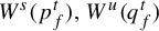 $W^s(p^t_f), W^u(q^t_f)$
contain an orbit
$W^s(p^t_f), W^u(q^t_f)$
contain an orbit
 $\Gamma ^t$
of corank-2 tangency. Then, for any integers
$\Gamma ^t$
of corank-2 tangency. Then, for any integers
 $\tilde n_1,\ldots ,\tilde n_h$
 $(0\le \tilde n_t\le r)$
, there exists a finite-parameter
$(0\le \tilde n_t\le r)$
, there exists a finite-parameter
 $C^{\infty }$
family
$C^{\infty }$
family
 $\mathcal F_{\varepsilon }$
such that
$\mathcal F_{\varepsilon }$
such that
 $\mathcal F_{0}=\mathrm {id}$
and the family
$\mathcal F_{0}=\mathrm {id}$
and the family
 $\mathcal F_{\varepsilon } \circ f$
perturbs the orbits
$\mathcal F_{\varepsilon } \circ f$
perturbs the orbits
 $\Gamma ^1,\ldots ,\Gamma ^h$
freely and independently up to orders
$\Gamma ^1,\ldots ,\Gamma ^h$
freely and independently up to orders
 $\tilde n_1,\ldots ,\tilde n_h$
. If all
$\tilde n_1,\ldots ,\tilde n_h$
. If all
 $\tilde n_t \le r-1$
, then the family
$\tilde n_t \le r-1$
, then the family
 $\mathcal F_{\varepsilon }$
can be chosen analytic.
$\mathcal F_{\varepsilon }$
can be chosen analytic.
Proof.
Construction of
 $C^{\infty }$
map
$C^{\infty }$
map
 $\mathcal F_{\varepsilon }$
. Let the basic set
$\mathcal F_{\varepsilon }$
. Let the basic set
 $\Omega _f$
have type
$\Omega _f$
have type
 $(k_s,k_u)$
. Fix points
$(k_s,k_u)$
. Fix points
 $M^1\in \Gamma ^1,\ldots ,M^h\in \Gamma ^h$
and sufficiently small
$M^1\in \Gamma ^1,\ldots ,M^h\in \Gamma ^h$
and sufficiently small
 $\rho>0$
such that neighbourhoods of the points
$\rho>0$
such that neighbourhoods of the points
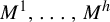 $M^1,\ldots ,M^h$
of size
$M^1,\ldots ,M^h$
of size
 $2\rho $
do not intersect pairwise. In these neighbourhoods, we introduce coordinates such that the equations of
$2\rho $
do not intersect pairwise. In these neighbourhoods, we introduce coordinates such that the equations of
 $W^s(p^t_f)$
and
$W^s(p^t_f)$
and
 $W^u(q^t_f)$
are given by equation (6).
$W^u(q^t_f)$
are given by equation (6).
We define
 $C^{\infty }$
-smooth cut-off functions
$C^{\infty }$
-smooth cut-off functions
 $\xi ^1_{\rho },\ldots ,\xi ^h_{\rho }$
acting from
$\xi ^1_{\rho },\ldots ,\xi ^h_{\rho }$
acting from
 $\mathbb R^k$
to
$\mathbb R^k$
to
 $\mathbb R$
such that
$\mathbb R$
such that
 $\xi ^t_{\rho }$
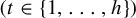 $(t\in \{1,\ldots ,h\})$
is equal to one inside the
$(t\in \{1,\ldots ,h\})$
is equal to one inside the
 $\rho $
-ball
$\rho $
-ball
 $B^1_{M^t}$
and vanishes identically outside the
$B^1_{M^t}$
and vanishes identically outside the
 $2\rho $
-ball
$2\rho $
-ball
 $B^2_{M^t}$
(the balls
$B^2_{M^t}$
(the balls
 $B^1_{M^t}, B^2_{M^t}$
are centred at the point
$B^1_{M^t}, B^2_{M^t}$
are centred at the point
 $M^t$
). Let
$M^t$
). Let
 $\mathcal F_{\varepsilon }$
be a
$\mathcal F_{\varepsilon }$
be a
 $C^{\infty }$
map that is an identity map outside the
$C^{\infty }$
map that is an identity map outside the
 $2\rho $
-balls
$2\rho $
-balls
 $B^2_{M^1},\ldots ,B^2_{M^h}$
and inside each ball,
$B^2_{M^1},\ldots ,B^2_{M^h}$
and inside each ball,
 $B^2_{M^t}$
acts as
$B^2_{M^t}$
acts as
 $$ \begin{align*} \begin{aligned} &(x_1,\ldots,x_{k_s},y_1,\ldots,y_{k_u})\\ &\quad\mapsto \bigg(x_1,\ldots,x_{k_s},y_1+\xi^t_{\rho}(x_1,\ldots,x_{k_s},y_1,\ldots,y_{k_u})\cdot \sum\limits_{j=0}^{\tilde n_t}\sum\limits_{i=0}^{j} \eta^t_{1,j,i} x_1^{j-i} x_2^{i},\\ &\qquad\qquad y_2+\xi^t_{\rho}(x_1,\ldots,x_{k_s},y_1,\ldots,y_{k_u})\cdot \sum\limits_{j=0}^{\tilde n_t}\sum\limits_{i=0}^{j} \eta^t_{2,j,i} x_1^{j-i} x_2^{i},y_3,\ldots,y_{k_u}\bigg), \end{aligned} \end{align*} $$
where
 $\varepsilon =(\overline \eta ^{1}_{\tilde n_1},\ldots ,\overline \eta ^{h}_{\tilde n_h})$
is a vector of parameters that runs a small ball centred at
$\varepsilon =(\overline \eta ^{1}_{\tilde n_1},\ldots ,\overline \eta ^{h}_{\tilde n_h})$
is a vector of parameters that runs a small ball centred at
 $\varepsilon =0$
. By construction, the map
$\varepsilon =0$
. By construction, the map
 $\mathcal F_{\varepsilon }$
is equal to the identity map everywhere at
$\mathcal F_{\varepsilon }$
is equal to the identity map everywhere at
 $\varepsilon =0$
.
$\varepsilon =0$
.
Consider the family
 $\mathcal F_{\varepsilon }\circ f$
. In this family, for each
$\mathcal F_{\varepsilon }\circ f$
. In this family, for each
 $t\in \{1,\ldots ,h\}$
near
$t\in \{1,\ldots ,h\}$
near
 $M^t$
, the equation for
$M^t$
, the equation for
 $W^s(p^t_{\varepsilon })$
does not change, while the equation for
$W^s(p^t_{\varepsilon })$
does not change, while the equation for
 $W^u(q^t_{\varepsilon })$
has the form
$W^u(q^t_{\varepsilon })$
has the form
 $$ \begin{align*} \begin{aligned} W^u(q^t_{\varepsilon})&=\bigg\{(y_1,y_2)=g^t_{1,\varepsilon}(x_1,x_2,y_3,\ldots,y_{k_u})+\sum\limits_{j=0}^{\tilde n_t}\sum\limits_{i=0}^{j} (\eta^t_{1,j,i},\eta^t_{2,j,i}) x_1^{j-i} x_2^{i}, \\ &\qquad(x_3,\ldots,x_{k_s})=g^t_{2,\varepsilon}(x_1,x_2,y_3,\ldots,y_{k_u})\bigg\}; \end{aligned} \end{align*} $$
therefore, the splitting function
 $G^t_{\varepsilon }$
is given by
$G^t_{\varepsilon }$
is given by
 $$ \begin{align*} \begin{aligned} &G^t_{\varepsilon}=G^t(x_1,x_2)+\sum\limits_{j=0}^{\tilde n_t}\sum\limits_{i=0}^{j} (\eta^t_{1,j,i},\eta^t_{2,j,i}) x_1^{j-i} x_2^{i}. \end{aligned} \end{align*} $$
By construction, the splitting coefficients
 $\eta ^t_{1,j,i}, \eta ^t_{2,j,i}$
 $(0\le j\le \tilde n_t\le r)$
depend smoothly on parameters
$(0\le j\le \tilde n_t\le r)$
depend smoothly on parameters
 $\varepsilon $
. Now, one can easily check that for the family
$\varepsilon $
. Now, one can easily check that for the family
 $\mathcal F_{\varepsilon }\circ f$
, the condition (7) holds (the corresponding matrix
$\mathcal F_{\varepsilon }\circ f$
, the condition (7) holds (the corresponding matrix
 ${\partial (\overline \eta ^{1}_{\tilde n_1},\ldots ,\overline \eta ^{h}_{\tilde n_h})}/{\partial \varepsilon }$
is the identity matrix); therefore, the family
${\partial (\overline \eta ^{1}_{\tilde n_1},\ldots ,\overline \eta ^{h}_{\tilde n_h})}/{\partial \varepsilon }$
is the identity matrix); therefore, the family
 $\mathcal F_{\varepsilon } \circ f$
perturbs the orbits
$\mathcal F_{\varepsilon } \circ f$
perturbs the orbits
 $\Gamma ^1,\ldots ,\Gamma ^h$
freely and independently up to orders
$\Gamma ^1,\ldots ,\Gamma ^h$
freely and independently up to orders
 $\tilde n_1,\ldots ,\tilde n_h$
.
$\tilde n_1,\ldots ,\tilde n_h$
.
Construction of real-analytic map
 $\mathcal F_{\varepsilon }$
. Let all
$\mathcal F_{\varepsilon }$
. Let all
 $\tilde n_t \le r-1$
. Let a map
$\tilde n_t \le r-1$
. Let a map
 $\mathcal F^{\mathrm {new}}_{\varepsilon }$
be a sufficiently close (in the
$\mathcal F^{\mathrm {new}}_{\varepsilon }$
be a sufficiently close (in the
 $C^r$
metric) analytic approximation of the map
$C^r$
metric) analytic approximation of the map
 $\mathcal F_{\varepsilon }$
. The condition (7) means that the matrix
$\mathcal F_{\varepsilon }$
. The condition (7) means that the matrix
 ${\partial (\overline \eta ^{1}_{\tilde n_1},\ldots ,\overline \eta ^{h}_{\tilde n_h})}/{\partial \varepsilon }$
has full rank. By construction, this matrix is quadratic (more precisely, it is of dimension
${\partial (\overline \eta ^{1}_{\tilde n_1},\ldots ,\overline \eta ^{h}_{\tilde n_h})}/{\partial \varepsilon }$
has full rank. By construction, this matrix is quadratic (more precisely, it is of dimension
 $N \times N$
, where
$N \times N$
, where
 $N=\sum \nolimits _{t=1}^h\chi _t(\overline \eta ^{t}_{\tilde n_t})$
), so we rewrite the condition (7) as
$N=\sum \nolimits _{t=1}^h\chi _t(\overline \eta ^{t}_{\tilde n_t})$
), so we rewrite the condition (7) as
 $\det ({\partial (\overline \eta ^{1}_{\tilde n_1},\ldots ,\overline \eta ^{h}_{\tilde n_h})}/{\partial \varepsilon }\not =0$
. Clearly, this condition is preserved for the family
$\det ({\partial (\overline \eta ^{1}_{\tilde n_1},\ldots ,\overline \eta ^{h}_{\tilde n_h})}/{\partial \varepsilon }\not =0$
. Clearly, this condition is preserved for the family
 $\mathcal F^{\mathrm {new}}_{\varepsilon }\circ f$
, so this family perturbs the orbits
$\mathcal F^{\mathrm {new}}_{\varepsilon }\circ f$
, so this family perturbs the orbits
 $\Gamma ^1,\ldots ,\Gamma ^h$
freely and independently up to orders
$\Gamma ^1,\ldots ,\Gamma ^h$
freely and independently up to orders
 $\tilde n_1,\ldots ,\tilde n_h$
.
$\tilde n_1,\ldots ,\tilde n_h$
.
Lemma 2.7 entails the following corollary.
Corollary 2.8. Let a
 $C^r$
map f, where
$C^r$
map f, where
 $r=2,\ldots ,\infty ,\omega $
, have a basic set
$r=2,\ldots ,\infty ,\omega $
, have a basic set
 $\Omega _f$
. Let
$\Omega _f$
. Let
 $p^1_f,q^1_f,\ldots ,p^h_f,q^h_f\in \Omega _f$
be points such that for each
$p^1_f,q^1_f,\ldots ,p^h_f,q^h_f\in \Omega _f$
be points such that for each
 $t\in \{1,\ldots ,h\}$
, the manifolds
$t\in \{1,\ldots ,h\}$
, the manifolds
 $W^s(p^t_f), W^u(q^t_f)$
contain an orbit
$W^s(p^t_f), W^u(q^t_f)$
contain an orbit
 $\Gamma ^t$
of corank-2 tangency of order
$\Gamma ^t$
of corank-2 tangency of order
 $n_t$
. Then, there exists a finite-parameter analytic family
$n_t$
. Then, there exists a finite-parameter analytic family
 $\mathcal F_{\varepsilon }$
such that
$\mathcal F_{\varepsilon }$
such that
 $\mathcal F_{0}=\mathrm {id}$
and in the family
$\mathcal F_{0}=\mathrm {id}$
and in the family
 $\mathcal F_{\varepsilon } \circ f$
, the tangencies
$\mathcal F_{\varepsilon } \circ f$
, the tangencies
 $\Gamma ^1,\ldots ,\Gamma ^h$
split freely and independently.
$\Gamma ^1,\ldots ,\Gamma ^h$
split freely and independently.
Proof. The proof of the corollary repeats verbatim the proof of Lemma 2.7 if we put
 $\tilde n_1=n_1,\ldots ,\tilde n_h=n_h$
in it.
$\tilde n_1=n_1,\ldots ,\tilde n_h=n_h$
in it.
Lemma 2.9. Let a
 $C^r$
map
$C^r$
map
 $f_0$
, where
$f_0$
, where
 $r=2,\ldots ,\infty ,\omega $
, have a non-trivial basic set
$r=2,\ldots ,\infty ,\omega $
, have a non-trivial basic set
 $\Omega _{f_0}$
. Let
$\Omega _{f_0}$
. Let
 $p_{f_0},q_{f_0}\in \Omega _{f_0}$
be points such that
$p_{f_0},q_{f_0}\in \Omega _{f_0}$
be points such that
 $W^s(p_{f_0})$
and
$W^s(p_{f_0})$
and
 $W^u(q_{f_0})$
contain an orbit
$W^u(q_{f_0})$
contain an orbit
 $\Gamma $
of corank-2 tangency of order n, and let
$\Gamma $
of corank-2 tangency of order n, and let
 $\mathcal O^1_{f_0},\mathcal O^2_{f_0}\in \Omega _{f_0}$
be any two periodic orbits. Let the map
$\mathcal O^1_{f_0},\mathcal O^2_{f_0}\in \Omega _{f_0}$
be any two periodic orbits. Let the map
 $f_0$
be included in a finite-parameter
$f_0$
be included in a finite-parameter
 $C^r$
family of maps
$C^r$
family of maps
 $f_{\varepsilon }$
in which the tangency
$f_{\varepsilon }$
in which the tangency
 $\Gamma $
splits freely. Then, there exists arbitrarily small
$\Gamma $
splits freely. Then, there exists arbitrarily small
 $\varepsilon ^{*}$
such that
$\varepsilon ^{*}$
such that
 $W^s(\mathcal O^1_{f_{\varepsilon ^{*}}})$
and
$W^s(\mathcal O^1_{f_{\varepsilon ^{*}}})$
and
 $W^u(\mathcal O^2_{f_{\varepsilon ^{*}}})$
contain an orbit of corank-2 tangency of order n.
$W^u(\mathcal O^2_{f_{\varepsilon ^{*}}})$
contain an orbit of corank-2 tangency of order n.
Proof. Let the basic set
 $\Omega _{f_0}$
have type
$\Omega _{f_0}$
have type
 $(k_s,k_u)$
. Fix a point
$(k_s,k_u)$
. Fix a point
 $M\in \Gamma $
and introduce near this point coordinates
$M\in \Gamma $
and introduce near this point coordinates
 $(x_1,\ldots ,x_{k_s},y_1,\ldots ,y_{k_u})$
. Then, the equations of the manifolds
$(x_1,\ldots ,x_{k_s},y_1,\ldots ,y_{k_u})$
. Then, the equations of the manifolds
 $W^s(p_{f_\varepsilon })$
and
$W^s(p_{f_\varepsilon })$
and
 $W^u(q_{f_\varepsilon })$
near M can be written as
$W^u(q_{f_\varepsilon })$
near M can be written as
 $$ \begin{align} \begin{aligned} W^s(p_{f_\varepsilon})&=\{(y_1,\ldots,y_{k_u})=(0,\ldots,0)\},\\ W^u(q_{f_\varepsilon})&=\{(y_1,y_2)=g_{1,\varepsilon}(x_1,x_2,y_3,\ldots,y_{k_u}), (x_3,\ldots,x_{k_s})\\ &\quad\hspace{6pt}=g_{2,\varepsilon}(x_1,x_2,y_3,\ldots,y_{k_u})\}, \end{aligned} \end{align} $$
with the splitting function
 $G_{\varepsilon }$
given by
$G_{\varepsilon }$
given by
 $$ \begin{align*} \begin{aligned} &G_{\varepsilon}(x_1,x_2)=g_{1,\varepsilon}(x_1,x_2,0,\ldots,0)=\sum\limits_{j=0}^{n}\sum\limits_{i=0}^{j} (\eta_{1,j,i},\eta_{2,j,i}) x_1^{j-i} x_2^{i} +O(\|x\|^{n+1}). \end{aligned} \end{align*} $$
Here,
 $\eta _{1,j,i}, \eta _{2,j,i}$
are the splitting coefficients vanishing at
$\eta _{1,j,i}, \eta _{2,j,i}$
are the splitting coefficients vanishing at
 $\varepsilon =0$
; at the point
$\varepsilon =0$
; at the point
 $(x_1,x_2)=(0,0)$
, one has
$(x_1,x_2)=(0,0)$
, one has
 ${\partial ^{n+1} G_0}/{\partial x^{i'}_1\partial x^{j'}_2}\not =(0,0)$
for some pair
${\partial ^{n+1} G_0}/{\partial x^{i'}_1\partial x^{j'}_2}\not =(0,0)$
for some pair
 $i'\ge 0$
,
$i'\ge 0$
,
 $j'\ge 0$
such that
$j'\ge 0$
such that
 $i'+j'=n+1$
. The tangency
$i'+j'=n+1$
. The tangency
 $\Gamma $
splits freely as
$\Gamma $
splits freely as
 $\varepsilon $
varies, so
$\varepsilon $
varies, so
 $$ \begin{align} \begin{aligned} &\text{rank }\frac{\partial\overline\eta_n}{\partial\varepsilon}\bigg |_{\varepsilon=0}=\chi(\overline\eta_{n}). \end{aligned} \end{align} $$
Let
 $\varepsilon =(\varepsilon _1,\ldots ,\varepsilon _l)$
and let
$\varepsilon =(\varepsilon _1,\ldots ,\varepsilon _l)$
and let
 $N=\chi (\overline \eta _{n})$
, so
$N=\chi (\overline \eta _{n})$
, so
 ${\partial \overline \eta _n}/{\partial \varepsilon } |_{\varepsilon =0}$
is ab
${\partial \overline \eta _n}/{\partial \varepsilon } |_{\varepsilon =0}$
is ab
 $N\times l$
matrix. The condition (9) means that this matrix has full rank, that is, it has non-zero minor determinant of order N. By renumbering parameters
$N\times l$
matrix. The condition (9) means that this matrix has full rank, that is, it has non-zero minor determinant of order N. By renumbering parameters
 $\varepsilon _1,\ldots ,\varepsilon _l$
, we get
$\varepsilon _1,\ldots ,\varepsilon _l$
, we get
 $$ \begin{align} \begin{aligned} &\det\frac{\partial\overline\eta_n}{\partial(\varepsilon_1,\ldots,\varepsilon_N)}\bigg|_{\varepsilon=0}\not=0. \end{aligned} \end{align} $$
Since the periodic orbits
 $\mathcal O^1_{f_{\varepsilon }}$
,
$\mathcal O^1_{f_{\varepsilon }}$
,
 $\mathcal O^2_{f_{\varepsilon }}$
belong to
$\mathcal O^2_{f_{\varepsilon }}$
belong to
 $\Omega _{f_{\varepsilon }}$
, the manifolds
$\Omega _{f_{\varepsilon }}$
, the manifolds
 $W^s(\mathcal O^1_{f_{\varepsilon }})$
and
$W^s(\mathcal O^1_{f_{\varepsilon }})$
and
 $W^u(\mathcal O^2_{f_{\varepsilon }})$
accumulate to
$W^u(\mathcal O^2_{f_{\varepsilon }})$
accumulate to
 $W^s(p_{f_\varepsilon })$
and
$W^s(p_{f_\varepsilon })$
and
 $W^u(q_{f_\varepsilon })$
, respectively. Therefore, we can write the equations of
$W^u(q_{f_\varepsilon })$
, respectively. Therefore, we can write the equations of
 $W^s(\mathcal O^1_{f_{\varepsilon }})$
and
$W^s(\mathcal O^1_{f_{\varepsilon }})$
and
 $W^u(\mathcal O^2_{f_{\varepsilon }})$
in a small neighbourhood of M as
$W^u(\mathcal O^2_{f_{\varepsilon }})$
in a small neighbourhood of M as
 $$ \begin{align} \begin{aligned} W^s(\mathcal O^1_{f_{\varepsilon}})&=\{(y_1,y_2)=\rho_{3,\varepsilon}(x_1,\ldots,x_{k_s}), (y_3,\ldots,y_{k_u})=\rho_{4,\varepsilon}(x_1,\ldots,x_{k_s})\},\\ W^u(\mathcal O^2_{f_{\varepsilon}})&=\{(y_1,y_2)=\rho_{1,\varepsilon}(x_1,x_2,y_3,\ldots,y_{k_u}), (x_3,\ldots,x_{k_s})\\ &\quad\hspace{6pt}=\rho_{2,\varepsilon}(x_1,x_2,y_3,\ldots,y_{k_u})\}, \end{aligned} \end{align} $$
where
 $\rho _{3,\varepsilon }$
and
$\rho _{3,\varepsilon }$
and
 $\rho _{4,\varepsilon }$
are
$\rho _{4,\varepsilon }$
are
 $C^r$
-close to the zero function;
$C^r$
-close to the zero function;
 $\rho _{1,\varepsilon }$
and
$\rho _{1,\varepsilon }$
and
 $\rho _{2,\varepsilon }$
are
$\rho _{2,\varepsilon }$
are
 $C^r$
-close to
$C^r$
-close to
 $g_{1,\varepsilon }$
and
$g_{1,\varepsilon }$
and
 $g_{2,\varepsilon }$
, respectively.
$g_{2,\varepsilon }$
, respectively.
Make a change of variables
 $$ \begin{align*} \begin{aligned} (y_1,y_2)^{\mathrm{new}}&=(y_1,y_2)-\rho_{3,\varepsilon}(x_1,\ldots,x_{k_s}),\\ (y_3,\ldots,y_{k_u})^{\mathrm{new}}&=(y_3,\ldots,y_{k_u})-\rho_{4,\varepsilon}(x_1,\ldots,x_{k_s}). \end{aligned} \end{align*} $$
As a result, equation (8) takes the form
 $$ \begin{align*} \begin{aligned} W^s(p_{f_\varepsilon})&=\{(y_1,y_2)=-\rho_{3,\varepsilon}(x_1,\ldots,x_{k_s}), (y_3,\ldots,y_{k_u})=-\rho_{4,\varepsilon}(x_1,\ldots,x_{k_s})\},\\ W^u(q_{f_\varepsilon})&=\{(y_1,y_2)=-\rho_{3,\varepsilon}(x_1,\ldots,x_{k_s})\\&\quad\hspace{6pt}+g_{1,\varepsilon}(x_1,x_2,(y_3,\ldots,y_{k_u})+\rho_{4,\varepsilon}(x_1,\ldots,x_{k_s})),\\ &\quad\hspace{8pt} (x_3,\ldots,x_{k_s})=g_{2,\varepsilon}(x_1,x_2,(y_3,\ldots,y_{k_u})+\rho_{4,\varepsilon}(x_1,\ldots,x_{k_s}))\}, \end{aligned} \end{align*} $$
while equation (11) takes the form
 $$ \begin{align*} \begin{aligned} W^s(\mathcal O^1_{f_{\varepsilon}})&=\{(y_1,\ldots,y_{k_u})=(0,\ldots,0)\},\\ W^u(\mathcal O^2_{f_{\varepsilon}})&=\{(y_1,y_2)=-\rho_{3,\varepsilon}(x_1,\ldots,x_{k_s})\\&\quad\hspace{6pt}+\rho_{1,\varepsilon}(x_1,x_2,(y_3,\ldots,y_{k_u})+\rho_{4,\varepsilon}(x_1,\ldots,x_{k_s})),\\ &\quad\hspace{8pt}(x_3,\ldots,x_{k_s})=\rho_{2,\varepsilon}(x_1,x_2,(y_3,\ldots,y_{k_u})+\rho_{4,\varepsilon}(x_1,\ldots,x_{k_s}))\}. \end{aligned} \end{align*} $$
Recall that
 $\rho _{3,\varepsilon }$
and
$\rho _{3,\varepsilon }$
and
 $\rho _{4,\varepsilon }$
are
$\rho _{4,\varepsilon }$
are
 $C^r$
-close to the zero function. So, making use of the implicit function theorem, we rewrite
$C^r$
-close to the zero function. So, making use of the implicit function theorem, we rewrite
 $W^u(q_{f_\varepsilon })$
and
$W^u(q_{f_\varepsilon })$
and
 $W^u(\mathcal O^2_{f_{\varepsilon }})$
as
$W^u(\mathcal O^2_{f_{\varepsilon }})$
as
 $$ \begin{align*} \begin{aligned} W^u(q_{f_\varepsilon})&=\{(y_1,y_2)=\hat g_{1,\varepsilon}(x_1,x_2,y_3,\ldots,y_{k_u}), (x_3,\ldots,x_{k_s})\\&\quad\hspace{6pt}=\hat g_{2,\varepsilon}(x_1,x_2,y_3,\ldots,y_{k_u})\},\\ W^u(\mathcal O^2_{f_{\varepsilon}})&=\{(y_1,y_2)=\hat\rho_{1,\varepsilon}(x_1,x_2,y_3,\ldots,y_{k_u}), (x_3,\ldots,x_{k_s})\\&\quad\hspace{6pt}=\hat\rho_{2,\varepsilon}(x_1,x_2,y_3,\ldots,y_{k_u})\}, \end{aligned} \end{align*} $$
where
 $\hat g_{1,\varepsilon }, \hat g_{2,\varepsilon }$
are
$\hat g_{1,\varepsilon }, \hat g_{2,\varepsilon }$
are
 $C^r$
-close to
$C^r$
-close to
 $g_{1,\varepsilon }, g_{2,\varepsilon }$
, and
$g_{1,\varepsilon }, g_{2,\varepsilon }$
, and
 $\hat \rho _{1,\varepsilon }, \hat \rho _{2,\varepsilon }$
are
$\hat \rho _{1,\varepsilon }, \hat \rho _{2,\varepsilon }$
are
 $C^r$
-close to
$C^r$
-close to
 $\rho _{1,\varepsilon }, \rho _{2,\varepsilon }$
.
$\rho _{1,\varepsilon }, \rho _{2,\varepsilon }$
.
For all small
 $\varepsilon $
, we define the function
$\varepsilon $
, we define the function
 $P_{\varepsilon }$
as
$P_{\varepsilon }$
as
 $$ \begin{align*} \begin{aligned} &P_{\varepsilon}(x_1,x_2)=\hat\rho_{1,\varepsilon}(x_1,x_2,0,\ldots,0). \end{aligned} \end{align*} $$
It can be written as
 $$ \begin{align} \begin{aligned} &P_{\varepsilon}(x_1,x_2)=\sum\limits_{j=0}^{n}\sum\limits_{i=0}^{j} (\varrho_{1,j,i}, \varrho_{2,j,i}) x_1^{j-i} x_2^{i} +O(\|x\|^{n+1}), \end{aligned} \end{align} $$
where
 $\varrho _{1,j,i}$
and
$\varrho _{1,j,i}$
and
 $\varrho _{2,j,i}$
are smooth functions of
$\varrho _{2,j,i}$
are smooth functions of
 $\varepsilon $
. Denote as
$\varepsilon $
. Denote as
 $\overline \varrho _{n}$
the vector consisting of all the coefficients
$\overline \varrho _{n}$
the vector consisting of all the coefficients
 $\varrho _{1,j,i}$
,
$\varrho _{1,j,i}$
,
 $\varrho _{2,j,i}$
, and let
$\varrho _{2,j,i}$
, and let
 $\chi (\overline \varrho _{n})$
be the total number of the components of this vector. Previous arguments imply that
$\chi (\overline \varrho _{n})$
be the total number of the components of this vector. Previous arguments imply that
 $P_{\varepsilon }$
is
$P_{\varepsilon }$
is
 $C^r$
-close to
$C^r$
-close to
 $G_{\varepsilon }$
, so
$G_{\varepsilon }$
, so
 $\overline \varrho _{n}$
and
$\overline \varrho _{n}$
and
 $\overline \eta _{n}$
are close. Therefore, by equation (10), we obtain that
$\overline \eta _{n}$
are close. Therefore, by equation (10), we obtain that
 $$ \begin{align} \begin{aligned} &\det\frac{\partial\overline\varrho_n}{\partial(\varepsilon_1,\ldots,\varepsilon_N)}\bigg|_{\varepsilon=0}\not=0. \end{aligned} \end{align} $$
By equation (12), the map
 $f_{\varepsilon }$
has an orbit of corank-2 tangency of order not lower than n between
$f_{\varepsilon }$
has an orbit of corank-2 tangency of order not lower than n between
 $W^s(\mathcal O^1_{f_{\varepsilon }})$
and
$W^s(\mathcal O^1_{f_{\varepsilon }})$
and
 $W^u(\mathcal O^2_{f_{\varepsilon }})$
if
$W^u(\mathcal O^2_{f_{\varepsilon }})$
if
 $$ \begin{align} \begin{aligned} &\overline\varrho_n=0. \end{aligned} \end{align} $$
Making use of equation (13) and the implicit function theorem, we get that the solution to equation (14) is given by
 $$ \begin{align} \begin{aligned} &(\varepsilon_1,\ldots,\varepsilon_N)=\mathcal H(\varepsilon_{N+1},\ldots,\varepsilon_{l}), \end{aligned} \end{align} $$
where
 $\mathcal H$
is a
$\mathcal H$
is a
 $C^{r-n}$
function. By choosing small
$C^{r-n}$
function. By choosing small
 $\varepsilon ^{*}=(\varepsilon _1^{*},\ldots ,\varepsilon _l^{*})$
satisfying equation (15), we find an orbit of corank-2 tangency of order not lower than n between
$\varepsilon ^{*}=(\varepsilon _1^{*},\ldots ,\varepsilon _l^{*})$
satisfying equation (15), we find an orbit of corank-2 tangency of order not lower than n between
 $W^s(\mathcal O^1_{f_{\varepsilon ^{*}}})$
and
$W^s(\mathcal O^1_{f_{\varepsilon ^{*}}})$
and
 $W^u(\mathcal O^2_{f_{\varepsilon ^{*}}})$
. This tangency is exactly of order n, since due to the
$W^u(\mathcal O^2_{f_{\varepsilon ^{*}}})$
. This tangency is exactly of order n, since due to the
 $C^r$
-closeness of
$C^r$
-closeness of
 $P_{\varepsilon }$
and
$P_{\varepsilon }$
and
 $G_{\varepsilon }$
, at the point
$G_{\varepsilon }$
, at the point
 $(x_1,x_2)=(0,0)$
, one has
$(x_1,x_2)=(0,0)$
, one has
 ${\partial ^{n+1} P_{\varepsilon ^{*}}}/{\partial x^{i'}_1\partial x^{j'}_2}\not =(0,0)$
.
${\partial ^{n+1} P_{\varepsilon ^{*}}}/{\partial x^{i'}_1\partial x^{j'}_2}\not =(0,0)$
.
2.2 Abundance of high-order tangencies of corank 2 in the
$ABR^{*}$
-domain

Lemma 2.10. Let f be a
 $C^r$
map
$C^r$
map
 $(r=2,\ldots ,\infty ,\omega )$
from the
$(r=2,\ldots ,\infty ,\omega )$
from the
 $ABR^{*}$
-domain, that is, f has homoclinically related bi-focus periodic orbit
$ABR^{*}$
-domain, that is, f has homoclinically related bi-focus periodic orbit
 $L_{f}$
and non-trivial basic set
$L_{f}$
and non-trivial basic set
 $\Lambda _{f}$
exhibiting
$\Lambda _{f}$
exhibiting
 $C^2$
-robust tangency of corank 2. Then, arbitrarily
$C^2$
-robust tangency of corank 2. Then, arbitrarily
 $C^r$
-close to f, there exists a map g such that
$C^r$
-close to f, there exists a map g such that
 $W^s(L_g)$
and
$W^s(L_g)$
and
 $W^u(L_g)$
contain h orbits
$W^u(L_g)$
contain h orbits
 $\Gamma ^1,\ldots ,\Gamma ^h$
of corank-2 homoclinic tangency, where h can be chosen to be any natural number.
$\Gamma ^1,\ldots ,\Gamma ^h$
of corank-2 homoclinic tangency, where h can be chosen to be any natural number.
Proof. Since
 $\Lambda _{f}$
and
$\Lambda _{f}$
and
 $L_{f}$
are homoclinically related, there exists a basic set
$L_{f}$
are homoclinically related, there exists a basic set
 $\Omega _{f}$
containing them. It entails that
$\Omega _{f}$
containing them. It entails that
 $W^s(L_{f})$
and
$W^s(L_{f})$
and
 $W^u(L_{f})$
accumulate to stable manifold and unstable manifold, respectively, of every point from
$W^u(L_{f})$
accumulate to stable manifold and unstable manifold, respectively, of every point from
 $\Lambda _{f}$
. Moreover, this property holds for all maps that are
$\Lambda _{f}$
. Moreover, this property holds for all maps that are
 $C^{r}$
-close to the map f.
$C^{r}$
-close to the map f.
The map f belongs to the
 $ABR^{*}$
-domain; therefore, it has an orbit
$ABR^{*}$
-domain; therefore, it has an orbit
 $\Gamma ^0$
of corank-2 tangency between
$\Gamma ^0$
of corank-2 tangency between
 $W^s(p^0_f)$
and
$W^s(p^0_f)$
and
 $W^u(q^0_f)$
, where
$W^u(q^0_f)$
, where
 $p^0_f$
,
$p^0_f$
,
 $q^0_f$
are some points in
$q^0_f$
are some points in
 $\Lambda _{f}$
. By Lemma 2.7, we include the map f in a finite-parameter
$\Lambda _{f}$
. By Lemma 2.7, we include the map f in a finite-parameter
 $C^r$
family that perturbs the orbit
$C^r$
family that perturbs the orbit
 $\Gamma ^0$
freely up to order
$\Gamma ^0$
freely up to order
 $2$
. First, if the tangency
$2$
. First, if the tangency
 $\Gamma ^0$
is not quadratic, then we make it quadratic by slightly varying parameters in this family. After that, applying Lemma 2.9, in the same family, arbitrarily
$\Gamma ^0$
is not quadratic, then we make it quadratic by slightly varying parameters in this family. After that, applying Lemma 2.9, in the same family, arbitrarily
 $C^r$
-close to f, we find a map
$C^r$
-close to f, we find a map
 $f_1$
that has an orbit
$f_1$
that has an orbit
 $\Gamma ^1$
of corank-2 homoclinic tangency between
$\Gamma ^1$
of corank-2 homoclinic tangency between
 $W^s(L_{f_1})$
and
$W^s(L_{f_1})$
and
 $W^u(L_{f_1})$
. Also, since the map
$W^u(L_{f_1})$
. Also, since the map
 $f_1$
belongs to the
$f_1$
belongs to the
 $ABR^{*}$
-domain, it has an orbit
$ABR^{*}$
-domain, it has an orbit
 $\Gamma ^{00}$
of corank-2 tangency between
$\Gamma ^{00}$
of corank-2 tangency between
 $W^s(p^1_{f_1})$
and
$W^s(p^1_{f_1})$
and
 $W^u(q^1_{f_1})$
, where
$W^u(q^1_{f_1})$
, where
 $p^1_{f_1},q^1_{f_1}\in \Lambda _{f_1}$
.
$p^1_{f_1},q^1_{f_1}\in \Lambda _{f_1}$
.
Again, making use of Lemma 2.7, we include the map
 $f_1$
in a finite-parameter
$f_1$
in a finite-parameter
 $C^r$
family that perturbs
$C^r$
family that perturbs
 $\Gamma ^{00}$
freely up to order
$\Gamma ^{00}$
freely up to order
 $2$
and in which the tangency
$2$
and in which the tangency
 $\Gamma ^1$
does not split. By Lemma 2.9, in this family, arbitrarily
$\Gamma ^1$
does not split. By Lemma 2.9, in this family, arbitrarily
 $C^r$
-close to
$C^r$
-close to
 $f_1$
, we find a map
$f_1$
, we find a map
 $f_2$
that has orbits
$f_2$
that has orbits
 $\Gamma ^1,\Gamma ^2$
of corank-2 homoclinic tangency between
$\Gamma ^1,\Gamma ^2$
of corank-2 homoclinic tangency between
 $W^s(L_{f_2})$
and
$W^s(L_{f_2})$
and
 $W^u(L_{f_2})$
, and an orbit
$W^u(L_{f_2})$
, and an orbit
 $\Gamma ^{000}$
of corank-2 tangency between
$\Gamma ^{000}$
of corank-2 tangency between
 $W^s(p^2_{f_2})$
and
$W^s(p^2_{f_2})$
and
 $W^u(q^2_{f_2})$
, where
$W^u(q^2_{f_2})$
, where
 $p^2_{f_2},q^2_{f_2}\in \Lambda _{f_2}$
.
$p^2_{f_2},q^2_{f_2}\in \Lambda _{f_2}$
.
Performing this procedure h times, we obtain a map
 $g\equiv f_h$
that has h orbits
$g\equiv f_h$
that has h orbits
 $\Gamma ^1,\ldots ,\Gamma ^h$
of corank-2 homoclinic tangency between
$\Gamma ^1,\ldots ,\Gamma ^h$
of corank-2 homoclinic tangency between
 $W^s(L_{g})$
and
$W^s(L_{g})$
and
 $W^u(L_{g})$
. By construction, the whole perturbation can be chosen arbitrarily small in the
$W^u(L_{g})$
. By construction, the whole perturbation can be chosen arbitrarily small in the
 $C^{r}$
topology.
$C^{r}$
topology.
Proof of Theorem 1.4
Let a
 $C^r$
map
$C^r$
map
 $f\in ABR^{*}$
-domain
$f\in ABR^{*}$
-domain
 $(r=2,\ldots ,\infty ,\omega )$
, that is, f has a homoclinically related bi-focus periodic orbit
$(r=2,\ldots ,\infty ,\omega )$
, that is, f has a homoclinically related bi-focus periodic orbit
 $L_f$
and non-trivial basic set
$L_f$
and non-trivial basic set
 $\Lambda _f$
exhibiting
$\Lambda _f$
exhibiting
 $C^2$
-robust tangency of corank 2. By definition, there exists a compact set
$C^2$
-robust tangency of corank 2. By definition, there exists a compact set
 $\mathcal L\subset W^s(\Lambda _f)\cup W^u(\Lambda _f)$
with the following property: given any compact neighbourhood U of
$\mathcal L\subset W^s(\Lambda _f)\cup W^u(\Lambda _f)$
with the following property: given any compact neighbourhood U of
 $\mathcal L$
, there exists a
$\mathcal L$
, there exists a
 $C^2$
neighbourhood
$C^2$
neighbourhood
 $\mathcal U$
of f such that for any map
$\mathcal U$
of f such that for any map
 $g\in \mathcal U$
, the manifolds
$g\in \mathcal U$
, the manifolds
 $W^s(\Lambda _g)$
and
$W^s(\Lambda _g)$
and
 $W^u(\Lambda _g)$
contain an orbit of corank-
$W^u(\Lambda _g)$
contain an orbit of corank-
 $2$
tangency lying entirely in U. We choose U in such a way that it does not intersect with the bi-focus orbit
$2$
tangency lying entirely in U. We choose U in such a way that it does not intersect with the bi-focus orbit
 $L_f$
, and obtain some neighbourhood
$L_f$
, and obtain some neighbourhood
 $\mathcal U$
of f with the property above. Further in the proof, as in §1.1.2, for simplicity of notation, we omit the dependence on a map in the subscript. We will consider that the map f is real-analytic (if f is only smooth, then arbitrarily
$\mathcal U$
of f with the property above. Further in the proof, as in §1.1.2, for simplicity of notation, we omit the dependence on a map in the subscript. We will consider that the map f is real-analytic (if f is only smooth, then arbitrarily
 $C^r$
-close to f, one can always find a map
$C^r$
-close to f, one can always find a map
 $f^{\mathrm {new}}$
that is real-analytic).
$f^{\mathrm {new}}$
that is real-analytic).
Let
 $\Omega $
be some basic set containing L and
$\Omega $
be some basic set containing L and
 $\Lambda $
. Let
$\Lambda $
. Let
 $n_1,n_2,\ldots $
be an infinite sequence of natural numbers and let
$n_1,n_2,\ldots $
be an infinite sequence of natural numbers and let
 $(\mathcal O^{1,1};\mathcal O^{1,2}),(\mathcal O^{2,1};\mathcal O^{2,2}),(\mathcal O^{3,1};\mathcal O^{3,2}),\ldots $
be an infinite sequence of pairs of periodic orbits from the basic set
$(\mathcal O^{1,1};\mathcal O^{1,2}),(\mathcal O^{2,1};\mathcal O^{2,2}),(\mathcal O^{3,1};\mathcal O^{3,2}),\ldots $
be an infinite sequence of pairs of periodic orbits from the basic set
 $\Omega $
. We choose these sequences as follows: for any periodic orbits
$\Omega $
. We choose these sequences as follows: for any periodic orbits
 $\mathcal O^1,\mathcal O^2$
from
$\mathcal O^1,\mathcal O^2$
from
 $\Omega $
and any natural number n, there exists k such that
$\Omega $
and any natural number n, there exists k such that
 $\mathcal O^1=\mathcal O^{k,1}$
,
$\mathcal O^1=\mathcal O^{k,1}$
,
 $\mathcal O^2=\mathcal O^{k,2}$
and
$\mathcal O^2=\mathcal O^{k,2}$
and
 $n=n_k$
. We will show that there exists a perturbation of f that does not lead out of the neighbourhood
$n=n_k$
. We will show that there exists a perturbation of f that does not lead out of the neighbourhood
 $\mathcal U$
and the
$\mathcal U$
and the
 $ABR^{*}$
-domain, and gives the map with an infinite sequence of orbits of homoclinic/heteroclinic corank-2 tangency, and these are exactly the tangencies of orders
$ABR^{*}$
-domain, and gives the map with an infinite sequence of orbits of homoclinic/heteroclinic corank-2 tangency, and these are exactly the tangencies of orders
 $n_k$
between the manifolds
$n_k$
between the manifolds
 $W^s(\mathcal O^{k,1})$
and
$W^s(\mathcal O^{k,1})$
and
 $W^u(\mathcal O^{k,2})$
, where
$W^u(\mathcal O^{k,2})$
, where
 $k\in \mathbb N$
. This perturbation can be as small as we need (in the
$k\in \mathbb N$
. This perturbation can be as small as we need (in the
 $C^{\omega }$
topology). The existence of such perturbation immediately provides a proof of the theorem (one should allow the numbers
$C^{\omega }$
topology). The existence of such perturbation immediately provides a proof of the theorem (one should allow the numbers
 $n_k$
to take all natural values infinitely many times).
$n_k$
to take all natural values infinitely many times).
Take an arbitrarily small
 $\delta>0$
and let
$\delta>0$
and let
 $\delta _k>0$
be such that
$\delta _k>0$
be such that
 $\delta _1+\delta _2+\cdots =\delta $
. We will construct a sequence of maps
$\delta _1+\delta _2+\cdots =\delta $
. We will construct a sequence of maps
 $f_k$
, where
$f_k$
, where
 $f_0\equiv f$
, such that
$f_0\equiv f$
, such that
 $f_k$
has an orbit of corank-2 tangency between
$f_k$
has an orbit of corank-2 tangency between
 $W^s(\Lambda )$
,
$W^s(\Lambda )$
,
 $W^u(\Lambda )$
(at least one, since
$W^u(\Lambda )$
(at least one, since
 $f_k\in \mathcal U$
) and k orbits of homoclinic/heteroclinic corank-2 tangency: one orbit of tangency of order
$f_k\in \mathcal U$
) and k orbits of homoclinic/heteroclinic corank-2 tangency: one orbit of tangency of order
 $n_1$
between
$n_1$
between
 $W^s(\mathcal O^{1,1})$
and
$W^s(\mathcal O^{1,1})$
and
 $W^u(\mathcal O^{1,2})$
, one orbit of tangency of order
$W^u(\mathcal O^{1,2})$
, one orbit of tangency of order
 $n_2$
between
$n_2$
between
 $W^s(\mathcal O^{2,1})$
and
$W^s(\mathcal O^{2,1})$
and
 $W^u(\mathcal O^{2,2})$
, etc. The maps
$W^u(\mathcal O^{2,2})$
, etc. The maps
 $f_k$
will have the property that the distance between
$f_k$
will have the property that the distance between
 $f_{k+1}$
and
$f_{k+1}$
and
 $f_k$
will be less than
$f_k$
will be less than
 $\delta _k$
. The sequence of maps
$\delta _k$
. The sequence of maps
 $f_k$
will have a limit
$f_k$
will have a limit
 $f^{*}$
, which is at a distance less than
$f^{*}$
, which is at a distance less than
 $\delta $
from f, and possess the required sequence of orbits of corank-2 tangency.
$\delta $
from f, and possess the required sequence of orbits of corank-2 tangency.
Thus, to prove the theorem, we have to show that given a map
 $f_k$
with an orbit of corank-2 tangency between
$f_k$
with an orbit of corank-2 tangency between
 $W^s(\Lambda ),W^u(\Lambda )$
, and
$W^s(\Lambda ),W^u(\Lambda )$
, and
 $k\ge 0$
orbits of corank-2 tangency between the stable and unstable manifolds of periodic orbits from
$k\ge 0$
orbits of corank-2 tangency between the stable and unstable manifolds of periodic orbits from
 $\Omega $
, one can perturb it and get the map
$\Omega $
, one can perturb it and get the map
 $f_{k+1}$
with the following properties:
$f_{k+1}$
with the following properties:
-
(1)
$f_{k+1}$
has an orbit of corank-2 tangency between
$W^s(\Lambda )$
and
$W^u(\Lambda )$
; -
(2)
$f_{k+1}$
preserves k orbits of corank-2 tangencies along with their orders (these orbits are ‘continuations’ of the corresponding orbits of the map
$f_k$
); -
(3)
$f_{k+1}$
has one more orbit
$\Gamma $
of corank-2 tangency between
$W^s(\mathcal O^{k+1,1})$
and
$W^u(\mathcal O^{k+1,2})$
of the given order
$n_{k+1}$
.


We will construct such a perturbation of the map
 $f_k$
as a finite sequence of perturbations each of which can be made arbitrarily
$f_k$
as a finite sequence of perturbations each of which can be made arbitrarily
 $C^{\omega }$
-small. Therefore, the resulting perturbation will be of class
$C^{\omega }$
-small. Therefore, the resulting perturbation will be of class
 $C^{\omega }$
and of total size less than
$C^{\omega }$
and of total size less than
 $\delta _{k+1}$
.
$\delta _{k+1}$
.
By Lemma 2.10, perturbing the map
 $f_k$
, we create another map
$f_k$
, we create another map
 $\overline f_k$
such that it has an orbit of corank-2 tangency between
$\overline f_k$
such that it has an orbit of corank-2 tangency between
 $W^s(\Lambda )$
and
$W^s(\Lambda )$
and
 $W^u(\Lambda )$
(the perturbation does not lead out of the neighbourhood
$W^u(\Lambda )$
(the perturbation does not lead out of the neighbourhood
 $\mathcal U$
), and
$\mathcal U$
), and
 $h=2^{{(n_{k+1}-1)(n_{k+1}+4)}/{2}}$
orbits of corank-2 homoclinic tangency between
$h=2^{{(n_{k+1}-1)(n_{k+1}+4)}/{2}}$
orbits of corank-2 homoclinic tangency between
 $W^s(L)$
and
$W^s(L)$
and
 $W^u(L)$
. In addition, this perturbation does not split any given finite number of tangencies that the map
$W^u(L)$
. In addition, this perturbation does not split any given finite number of tangencies that the map
 $f_k$
has had. Applying Theorem 1.2 to the map
$f_k$
has had. Applying Theorem 1.2 to the map
 $\overline f_k$
, we get a map
$\overline f_k$
, we get a map
 $\tilde f_k$
with an orbit
$\tilde f_k$
with an orbit
 $\tilde \Gamma $
of corank-2 homoclinic tangency of order
$\tilde \Gamma $
of corank-2 homoclinic tangency of order
 $n_{k+1}$
between
$n_{k+1}$
between
 $W^s(L)$
and
$W^s(L)$
and
 $W^u(L)$
, while also keeping any given finite number of orbits of tangencies along with their orders.
$W^u(L)$
, while also keeping any given finite number of orbits of tangencies along with their orders.
Let us recall that the orbits
 $L, \mathcal O^{k+1,1}$
and
$L, \mathcal O^{k+1,1}$
and
 $\mathcal O^{k+1,2}$
belong to the same non-trivial basic set
$\mathcal O^{k+1,2}$
belong to the same non-trivial basic set
 $\Omega $
; therefore, invariant manifolds
$\Omega $
; therefore, invariant manifolds
 $W^s(\mathcal O^{k+1,1})$
and
$W^s(\mathcal O^{k+1,1})$
and
 $W^u(\mathcal O^{k+1,2})$
accumulate to invariant manifolds
$W^u(\mathcal O^{k+1,2})$
accumulate to invariant manifolds
 $W^s(L)$
and
$W^s(L)$
and
 $W^u(L)$
, respectively. Using Corollary 2.8, include the map
$W^u(L)$
, respectively. Using Corollary 2.8, include the map
 $\tilde f_k$
in an analytic finite-parameter family in which the tangency
$\tilde f_k$
in an analytic finite-parameter family in which the tangency
 $\tilde \Gamma $
splits freely. By Lemma 2.9, in this family, arbitrarily
$\tilde \Gamma $
splits freely. By Lemma 2.9, in this family, arbitrarily
 $C^{\omega }$
-close to
$C^{\omega }$
-close to
 $\tilde f_k$
, we find a map
$\tilde f_k$
, we find a map
 $f_{k+1}$
with the sought orbit
$f_{k+1}$
with the sought orbit
 $\Gamma $
of corank-2 tangency of order
$\Gamma $
of corank-2 tangency of order
 $n_{k+1}$
between
$n_{k+1}$
between
 $W^s(\mathcal O^{k+1,1})$
and
$W^s(\mathcal O^{k+1,1})$
and
 $W^u(\mathcal O^{k+1,2})$
. By construction, at least one point of the orbit
$W^u(\mathcal O^{k+1,2})$
. By construction, at least one point of the orbit
 $\Gamma $
is close to L (proximity to L is controlled by the size of the perturbation that splits the tangency
$\Gamma $
is close to L (proximity to L is controlled by the size of the perturbation that splits the tangency
 $\tilde \Gamma $
), so
$\tilde \Gamma $
), so
 $\Gamma $
does not lie entirely in U. Moreover, the map
$\Gamma $
does not lie entirely in U. Moreover, the map
 $f_{k+1}$
belongs to
$f_{k+1}$
belongs to
 $\mathcal U$
, so it has an orbit
$\mathcal U$
, so it has an orbit
 $\Gamma '$
of corank-2 tangency between
$\Gamma '$
of corank-2 tangency between
 $W^s(\Lambda )$
and
$W^s(\Lambda )$
and
 $W^u(\Lambda )$
, lying entirely in U. Clearly, the orbits
$W^u(\Lambda )$
, lying entirely in U. Clearly, the orbits
 $\Gamma $
and
$\Gamma $
and
 $\Gamma '$
are different.
$\Gamma '$
are different.
Thus, we constructed a map
 $f_{k+1}$
that has an orbit
$f_{k+1}$
that has an orbit
 $\Gamma '$
of corank-2 tangency between
$\Gamma '$
of corank-2 tangency between
 $W^s(\Lambda )$
and
$W^s(\Lambda )$
and
 $W^u(\Lambda )$
, the sought orbit
$W^u(\Lambda )$
, the sought orbit
 $\Gamma $
of corank-2 tangency of order
$\Gamma $
of corank-2 tangency of order
 $n_{k+1}$
between
$n_{k+1}$
between
 $W^s(\mathcal O^{k+1,1})$
and
$W^s(\mathcal O^{k+1,1})$
and
 $W^u(\mathcal O^{k+1,2})$
, and preserves k orbits of corank-2 tangencies along with their orders (which are ‘continuations’ of the corresponding orbits of the map
$W^u(\mathcal O^{k+1,2})$
, and preserves k orbits of corank-2 tangencies along with their orders (which are ‘continuations’ of the corresponding orbits of the map
 $f_k$
).
$f_k$
).
This completes the proof of Theorem 1.4.
Proof of Theorem 1.5
Let f be a
 $C^r$
map
$C^r$
map
 $(r=2,\ldots ,\infty )$
from the
$(r=2,\ldots ,\infty )$
from the
 $ABR^{*}$
-domain. By Theorem 1.4, arbitrarily
$ABR^{*}$
-domain. By Theorem 1.4, arbitrarily
 $C^r$
-close to a map f there exists a real-analytic map g with a basic set
$C^r$
-close to a map f there exists a real-analytic map g with a basic set
 $\Omega _{g}$
such that for any pair of periodic orbits
$\Omega _{g}$
such that for any pair of periodic orbits
 $\mathcal O^1_g,\mathcal O^2_g\in \Omega _g$
, the stable manifold
$\mathcal O^1_g,\mathcal O^2_g\in \Omega _g$
, the stable manifold
 $W^s(\mathcal O^1_g)$
and the unstable manifold
$W^s(\mathcal O^1_g)$
and the unstable manifold
 $W^u(\mathcal O^2_g)$
contain infinitely many orbits of corank-2 tangency of every order. Among all these orbits, let us choose an infinite sequence
$W^u(\mathcal O^2_g)$
contain infinitely many orbits of corank-2 tangency of every order. Among all these orbits, let us choose an infinite sequence
 $\mathcal G$
consisting of all orbits with the following property:
$\mathcal G$
consisting of all orbits with the following property:
-
(1) if r is finite, then each orbit from
$\mathcal G$
is an orbit of corank-2 tangency of order
$n=r$
; -
(2) if
$r=\infty $
, then each orbit from
$\mathcal G$
is an orbit of corank-2 tangency of order n, where n is sufficiently large.


Next, for each orbit from
 $\mathcal G$
, we transform tangency to an intersection of stable and unstable manifolds by a two-dimensional disk. We do it using a perturbation that is arbitrarily small (in the
$\mathcal G$
, we transform tangency to an intersection of stable and unstable manifolds by a two-dimensional disk. We do it using a perturbation that is arbitrarily small (in the
 $C^r$
topology) and that is localized in an arbitrarily small given neighbourhood of one point of the orbit of tangency under consideration. Moreover, we localize these perturbations in such a way that they do not affect all other orbits of tangency from
$C^r$
topology) and that is localized in an arbitrarily small given neighbourhood of one point of the orbit of tangency under consideration. Moreover, we localize these perturbations in such a way that they do not affect all other orbits of tangency from
 $\mathcal G$
. As a result of sequential application of such perturbations, arbitrarily
$\mathcal G$
. As a result of sequential application of such perturbations, arbitrarily
 $C^r$
-close to g, we obtain a map
$C^r$
-close to g, we obtain a map
 $h\in ABR^{*}$
-domain such that it has non-trivial basic set
$h\in ABR^{*}$
-domain such that it has non-trivial basic set
 $\Omega _{h}$
in which the intersection of the stable and unstable manifolds of every pair of periodic orbits contains a two-dimensional disk. It completes the proof.
$\Omega _{h}$
in which the intersection of the stable and unstable manifolds of every pair of periodic orbits contains a two-dimensional disk. It completes the proof.
3 High-order tangencies of corank-2 to bi-focus periodic orbit
In this section, we prove Theorem 1.2. Let us emphasize that all the results in this section are independent of the
 $ABR^{*}$
-domain.
$ABR^{*}$
-domain.
In our proofs, we ‘split’ the dynamics of maps with homoclinic orbits into two parts, considering the so-called local and global maps. In §§3.1 and 3.2, we provide explicit formulae for these maps. In §3.3, we introduce the index of corank-2 tangency, which plays a leading role in the proof of Theorem 1.2, and reformulate some constructions from §2.1 in terms of the global maps. In §3.4, we describe the parametric families that we use in our proofs. In §3.5, we provide key Lemmas 3.10, 3.11, 3.12, which serve as a basis for obtaining high-order tangencies of corank 2. After it, we prove Theorem 1.2.
3.1 Local map
Let f be a
 $C^r$
map
$C^r$
map
 $(r=2,\ldots ,\infty ,\omega )$
with a bi-focus periodic orbit
$(r=2,\ldots ,\infty ,\omega )$
with a bi-focus periodic orbit
 $L_f=\{O_f,f(O_f),\ldots ,f^{b-1}(O_f)\}$
of period b. Denote by
$L_f=\{O_f,f(O_f),\ldots ,f^{b-1}(O_f)\}$
of period b. Denote by
 $\unicode{x3bb} _1,\ldots ,\unicode{x3bb} _{k_s}$
,
$\unicode{x3bb} _1,\ldots ,\unicode{x3bb} _{k_s}$
,
 $\gamma _1,\ldots ,\gamma _{k_u}$
the multipliers of
$\gamma _1,\ldots ,\gamma _{k_u}$
the multipliers of
 $L_f$
, and order them so that
$L_f$
, and order them so that
 $|\gamma _{k_u}|\ge \cdots \ge |\gamma _1|>1>|\unicode{x3bb} _1|\ge \cdots \ge | \unicode{x3bb} _{k_s}|>0$
. Denote
$|\gamma _{k_u}|\ge \cdots \ge |\gamma _1|>1>|\unicode{x3bb} _1|\ge \cdots \ge | \unicode{x3bb} _{k_s}|>0$
. Denote
 $\unicode{x3bb} _{1,2}=\unicode{x3bb} e^{\pm i\varphi }, \gamma _{1,2}=\gamma e^{\pm i\psi }$
, where
$\unicode{x3bb} _{1,2}=\unicode{x3bb} e^{\pm i\varphi }, \gamma _{1,2}=\gamma e^{\pm i\psi }$
, where
 $\varphi ,\psi \not =0,\pi $
, and
$\varphi ,\psi \not =0,\pi $
, and
 $\unicode{x3bb} =|\unicode{x3bb} _{1,2}|$
,
$\unicode{x3bb} =|\unicode{x3bb} _{1,2}|$
,
 $\gamma =|\gamma _{1,2}|$
. Note that the definition of a bi-focus periodic orbit entails that if
$\gamma =|\gamma _{1,2}|$
. Note that the definition of a bi-focus periodic orbit entails that if
 $L_f$
has non-leading multipliers (that is, the dimension of the ambient manifold is more than 4), then
$L_f$
has non-leading multipliers (that is, the dimension of the ambient manifold is more than 4), then
We will assume that
 $\unicode{x3bb} \gamma \not =1$
since this can always be achieved by adding a
$\unicode{x3bb} \gamma \not =1$
since this can always be achieved by adding a
 $C^r$
-small perturbation. We will consider the case
$C^r$
-small perturbation. We will consider the case
 $\unicode{x3bb} \gamma <1$
(if
$\unicode{x3bb} \gamma <1$
(if
 $\unicode{x3bb} \gamma>1$
, then it is sufficient to consider the map
$\unicode{x3bb} \gamma>1$
, then it is sufficient to consider the map
 $f^{-1}$
instead of f).
$f^{-1}$
instead of f).
Denote by
 $T_0$
the restriction of the Poincaré map
$T_0$
the restriction of the Poincaré map
 $f^b$
to a small neighbourhood U of the point
$f^b$
to a small neighbourhood U of the point
 $O_{f}$
. The map
$O_{f}$
. The map
 $T_0$
is called the local map. By
$T_0$
is called the local map. By
 $C^r$
change of coordinates, we put the origin at
$C^r$
change of coordinates, we put the origin at
 $O_f$
, and straighten the local stable manifold
$O_f$
, and straighten the local stable manifold
 $W^s_{\mathrm {loc}}(O_f)$
and the local unstable manifold
$W^s_{\mathrm {loc}}(O_f)$
and the local unstable manifold
 $W^u_{\mathrm {loc}}(O_f)$
. After this, the local map takes the form
$W^u_{\mathrm {loc}}(O_f)$
. After this, the local map takes the form
 $$ \begin{align} \begin{aligned} \overline x_1&=\unicode{x3bb}\cdot(x_1\cos(k\varphi)-x_2\sin(k\varphi))+\vartheta_1(x_1,x_2,y_1,y_2,u,v),\\ \overline x_2&=\unicode{x3bb}\cdot(x_1\sin(k\varphi)+x_2\cos(k\varphi))+\vartheta_2(x_1,x_2,y_1,y_2,u,v),\\ \overline y_1&=\gamma\cdot(y_1\cos(k\psi)-y_2\sin(k\psi))+\vartheta_3(x_1,x_2,y_1,y_2,u,v),\\ \overline y_2&=\gamma\cdot(y_1\sin(k\psi)+y_2\cos(k\psi))+\vartheta_4(x_1,x_2,y_1,y_2,u,v),\\ \overline u&=A u+\vartheta_5(x_1,x_2,y_1,y_2,u,v),\\ \overline v&=B v+\vartheta_6(x_1,x_2,y_1,y_2,u,v), \end{aligned} \end{align} $$
where
 $u\in \mathbb R^{k_s-2}, v\in \mathbb R^{k_u-2}$
, the eigenvalues of the matrices A and B are respectively the stable and unstable non-leading multipliers of the orbit
$u\in \mathbb R^{k_s-2}, v\in \mathbb R^{k_u-2}$
, the eigenvalues of the matrices A and B are respectively the stable and unstable non-leading multipliers of the orbit
 $L_{f}$
, and the nonlinearities
$L_{f}$
, and the nonlinearities
 $\vartheta $
satisfy
$\vartheta $
satisfy
 $$ \begin{align*} \begin{aligned} &\vartheta_{1,2,5}(0,0,y_1,y_2,0,v)\equiv0, \quad \vartheta_{3,4,6}(x_1,x_2,0,0,u,0)\equiv0.\\ \end{aligned} \end{align*} $$
Moreover, following [Reference Gonchenko, Shilnikov and Turaev26], we do some
 $C^r$
changes of coordinates to eliminate some nonlinear terms in equation (16) (so the iterations
$C^r$
changes of coordinates to eliminate some nonlinear terms in equation (16) (so the iterations
 $T_0^k$
are not too far from the iterations of the linearization). Specifically, the nonlinearities
$T_0^k$
are not too far from the iterations of the linearization). Specifically, the nonlinearities
 $\vartheta ^{\mathrm {new}}$
satisfy (below, we omit the superscript ‘new’)
$\vartheta ^{\mathrm {new}}$
satisfy (below, we omit the superscript ‘new’)
 $$ \begin{align} \begin{aligned} &\vartheta_{1,2}(x_1,x_2,0,0,u,0)\equiv0, \quad \vartheta_{3,4}(0,0,y_1,y_2,0,v)\equiv0,\\ \end{aligned} \end{align} $$
 $$ \begin{align} \begin{aligned} &\frac{\partial \vartheta_{1,2,5}}{\partial (x_1,x_2)}(0,0,y_1,y_2,0,v)\equiv0, \quad \frac{\partial \vartheta_{3,4,6}}{\partial (y_1,y_2)}(x_1,x_2,0,0,u,0)\equiv0.\\ \end{aligned} \end{align} $$
When the map
 $T_0$
is written in the obtained coordinates, we say that it is in the main normal form.
$T_0$
is written in the obtained coordinates, we say that it is in the main normal form.
Let
 $f_{\varepsilon }$
be a finite-parameter
$f_{\varepsilon }$
be a finite-parameter
 $C^r$
family of maps, where
$C^r$
family of maps, where
 $\varepsilon $
is a vector of parameters that runs a small ball centred at
$\varepsilon $
is a vector of parameters that runs a small ball centred at
 $\varepsilon =0$
and where
$\varepsilon =0$
and where
 $f_0=f$
. Since
$f_0=f$
. Since
 $f_0$
has a bi-focus periodic orbit
$f_0$
has a bi-focus periodic orbit
 $L_{f_0}$
, then this orbit persists for all small values of
$L_{f_0}$
, then this orbit persists for all small values of
 $\varepsilon $
. It depends smoothly on
$\varepsilon $
. It depends smoothly on
 $\varepsilon $
and its multipliers are
$\varepsilon $
and its multipliers are
 $C^{r-1}$
functions with respect to
$C^{r-1}$
functions with respect to
 $\varepsilon $
. For all small
$\varepsilon $
. For all small
 $\varepsilon $
, the local map
$\varepsilon $
, the local map
 $T_0$
is correctly defined and
$T_0$
is correctly defined and
 $O_{f_{\varepsilon }}$
is its fixed point. We consider such coordinates that for all small
$O_{f_{\varepsilon }}$
is its fixed point. We consider such coordinates that for all small
 $\varepsilon $
, the map
$\varepsilon $
, the map
 $T_0$
is written in the main normal form (see [Reference Gonchenko, Shilnikov and Turaev26]).
$T_0$
is written in the main normal form (see [Reference Gonchenko, Shilnikov and Turaev26]).
Let
 $(x_{k1},x_{k2},y_{k1},y_{k2}, u_k,v_k)=T_0^k(x_{01},x_{02},y_{01},y_{02}, u_0,v_0)$
. By [Reference Shilnikov43],
$(x_{k1},x_{k2},y_{k1},y_{k2}, u_k,v_k)=T_0^k(x_{01},x_{02},y_{01},y_{02}, u_0,v_0)$
. By [Reference Shilnikov43],
 $(x_{k1},x_{k2},y_{01}, y_{02}, u_k,v_0)$
are uniquely defined functions of
$(x_{k1},x_{k2},y_{01}, y_{02}, u_k,v_0)$
are uniquely defined functions of
 $(x_{01},x_{02},y_{k1},y_{k2}, u_0,v_k)$
. The formulae for the iterations of the local map
$(x_{01},x_{02},y_{k1},y_{k2}, u_0,v_k)$
. The formulae for the iterations of the local map
 $T_0$
are given by the following proposition.
$T_0$
are given by the following proposition.
Proposition 3.1. [Reference Gonchenko, Shilnikov and Turaev26, Lemma 7]
When the local map
 $T_0$
is brought to the main normal form, the following relations hold for all small
$T_0$
is brought to the main normal form, the following relations hold for all small
 $\varepsilon $
and all large k:
$\varepsilon $
and all large k:

where
![]() and
and
![]() are some constants such that
are some constants such that
 $0<\hat \unicode{x3bb} <\unicode{x3bb} $
,
$0<\hat \unicode{x3bb} <\unicode{x3bb} $
,
 $\hat \gamma>\gamma $
, and the functions
$\hat \gamma>\gamma $
, and the functions
 $\xi ^1_k,\xi ^2_k, \eta ^1_k,\eta ^2_k, \hat \xi _k, \hat \eta _k$
are uniformly bounded for all k, along with the derivatives up to the order
$\xi ^1_k,\xi ^2_k, \eta ^1_k,\eta ^2_k, \hat \xi _k, \hat \eta _k$
are uniformly bounded for all k, along with the derivatives up to the order
 $r-2$
.
$r-2$
.
Remark 3.2. The proof from [Reference Gonchenko, Shilnikov and Turaev26] (Lemma 7) directly implies that the constants
and
 $\hat \gamma $
can be chosen such that
$\hat \gamma $
can be chosen such that
3.2 Global map
Again, let f be a
 $C^r$
map
$C^r$
map
 $(r=2,\ldots ,\infty ,\omega )$
with a bi-focus periodic orbit
$(r=2,\ldots ,\infty ,\omega )$
with a bi-focus periodic orbit
 $L_f=\{O_f,f(O_f),\ldots ,f^{b-1}(O_f)\}$
of period b. Now, assume that the stable and unstable manifolds of
$L_f=\{O_f,f(O_f),\ldots ,f^{b-1}(O_f)\}$
of period b. Now, assume that the stable and unstable manifolds of
 $L_f$
contain an orbit
$L_f$
contain an orbit
 $\Gamma $
of corank-2 homoclinic tangency. The points of intersection of the homoclinic orbit
$\Gamma $
of corank-2 homoclinic tangency. The points of intersection of the homoclinic orbit
 $\Gamma $
with the neighbourhood U of the point
$\Gamma $
with the neighbourhood U of the point
 $O_f$
belong to local stable manifold
$O_f$
belong to local stable manifold
 $W^s_{\mathrm {loc}}(O_f)$
and local unstable manifold
$W^s_{\mathrm {loc}}(O_f)$
and local unstable manifold
 $W^u_{\mathrm {loc}}(O_f)$
, and converge to
$W^u_{\mathrm {loc}}(O_f)$
, and converge to
 $O_f$
at the forward and respectively backward iterations of the local map
$O_f$
at the forward and respectively backward iterations of the local map
 $T_0$
. Let
$T_0$
. Let
 ${M^{+}\in W^s_{\mathrm {loc}}(O_f)}$
and
${M^{+}\in W^s_{\mathrm {loc}}(O_f)}$
and
 $M^{-}\in W^u_{\mathrm {loc}}(O_f)$
be two points of the orbit
$M^{-}\in W^u_{\mathrm {loc}}(O_f)$
be two points of the orbit
 $\Gamma $
. Since the points
$\Gamma $
. Since the points
 $M^+$
and
$M^+$
and
 $M^-$
belong to the the same orbit, there exists a positive integer
$M^-$
belong to the the same orbit, there exists a positive integer
 $k_0$
such that
$k_0$
such that
 $M^{+}=f^{k_0}(M^{-})$
. Let
$M^{+}=f^{k_0}(M^{-})$
. Let
 $\Pi ^{+}$
and
$\Pi ^{+}$
and
 $\Pi ^{-}$
be some small neighbourhoods of
$\Pi ^{-}$
be some small neighbourhoods of
 $M^+$
and
$M^+$
and
 $M^-$
, respectively. The map
$M^-$
, respectively. The map
 $T_\Gamma \equiv f^{k_0}: \Pi ^-\rightarrow \Pi ^+$
is said to be the global map.
$T_\Gamma \equiv f^{k_0}: \Pi ^-\rightarrow \Pi ^+$
is said to be the global map.
If the orbit
 $L_f$
has non-leading multipliers, then we require the fulfilment of certain genericity conditions regarding the geometry of the homoclinic tangency. We will denote the eigensubspace of the linear part of the local map
$L_f$
has non-leading multipliers, then we require the fulfilment of certain genericity conditions regarding the geometry of the homoclinic tangency. We will denote the eigensubspace of the linear part of the local map
 $T_0$
corresponding to the multipliers:
$T_0$
corresponding to the multipliers:
-
(1)
$\unicode{x3bb} _3,\ldots ,\unicode{x3bb} _{k_s}$
(non-leading stable) by
$\mathcal E^{ss}$
and
$\gamma _3,\ldots ,\gamma _{k_u}$
(non-leading unstable) by
$\mathcal E^{uu}$
; -
(2)
$\gamma _1,\gamma _2,\unicode{x3bb} _1,\ldots ,\unicode{x3bb} _{k_s}$
(leading unstable and stable) by
$\mathcal E^{se}$
and
$\unicode{x3bb} _1,\unicode{x3bb} _2,\gamma _1,\ldots ,\gamma _{k_u}$
(leading stable and unstable) by
$\mathcal E^{ue}$
.


There is an invariant
 $C^r$
-smooth manifold
$C^r$
-smooth manifold
 $W^{ss}(O_f)\subset W^s(O_f)$
that is tangent to
$W^{ss}(O_f)\subset W^s(O_f)$
that is tangent to
 $\mathcal E^{ss}$
. Similarly, there is an invariant
$\mathcal E^{ss}$
. Similarly, there is an invariant
 $C^r$
-smooth manifold
$C^r$
-smooth manifold
 $W^{uu}(O_f)\subset W^u(O_f)$
, tangent to
$W^{uu}(O_f)\subset W^u(O_f)$
, tangent to
 $\mathcal E^{uu}$
. Recall (see e.g. [Reference Shilnikov, Shilnikov, Turaev and Chua44]) that
$\mathcal E^{uu}$
. Recall (see e.g. [Reference Shilnikov, Shilnikov, Turaev and Chua44]) that
 $W^{ss}(O_f)$
and
$W^{ss}(O_f)$
and
 $W^{uu}(O_f)$
are uniquely included in invariant
$W^{uu}(O_f)$
are uniquely included in invariant
 $C^r$
-smooth foliations
$C^r$
-smooth foliations
 $F^{ss}$
and
$F^{ss}$
and
 $F^{uu}$
on
$F^{uu}$
on
 $W^s(O_f)$
and
$W^s(O_f)$
and
 $W^u(O_f)$
, respectively. Also, there exist invariant manifolds
$W^u(O_f)$
, respectively. Also, there exist invariant manifolds
 $W^{se}(O_f)$
and
$W^{se}(O_f)$
and
 $W^{ue}(O_f)$
(at least
$W^{ue}(O_f)$
(at least
 $C^1$
-smooth) that are tangent to
$C^1$
-smooth) that are tangent to
 $\mathcal E^{se}$
and
$\mathcal E^{se}$
and
 $\mathcal E^{ue}$
, respectively. The manifolds
$\mathcal E^{ue}$
, respectively. The manifolds
 $W^{se}(O_f)$
and
$W^{se}(O_f)$
and
 $W^{ue}(O_f)$
are not unique, but
$W^{ue}(O_f)$
are not unique, but
 $\mathcal T_{M^+}(W^{se}(O_f))$
and
$\mathcal T_{M^+}(W^{se}(O_f))$
and
 $\mathcal T_{M^-}(W^{ue}(O_f))$
are defined uniquely. The genericity conditions are:
$\mathcal T_{M^-}(W^{ue}(O_f))$
are defined uniquely. The genericity conditions are:
-
(C1)
$T_\Gamma (W^{ue}(O_f))$
is transverse to the leaf
$l^{ss}$
of
$F^{ss}$
that passes through
$M^+$
; -
(C2)
$T_\Gamma ^{-1}(W^{se}(O_f))$
is transverse to the leaf
$l^{uu}$
of
$F^{uu}$
that passes through
$M^-$
.


Note that since the manifolds and foliations are invariant, conditions (C1) and (C2) are independent of the choice of the homoclinic points
 $M^+$
and
$M^+$
and
 $M^-$
. Obviously, these conditions can be fulfilled after an arbitrary
$M^-$
. Obviously, these conditions can be fulfilled after an arbitrary
 $C^r$
-small perturbation. A detailed discussion can be found in [Reference Turaev50].
$C^r$
-small perturbation. A detailed discussion can be found in [Reference Turaev50].
Further in this section, we will work in coordinates
 $(x_1,x_2,y_1,y_2,u,v)$
for which the local map
$(x_1,x_2,y_1,y_2,u,v)$
for which the local map
 $T_0$
is in the main normal form. Then, the manifolds
$T_0$
is in the main normal form. Then, the manifolds
 $W^s_{\mathrm {loc}}(O_f)$
,
$W^s_{\mathrm {loc}}(O_f)$
,
 $W^u_{\mathrm {loc}}(O_f)$
are straightened and given by
$W^u_{\mathrm {loc}}(O_f)$
are straightened and given by
 $$ \begin{align} \begin{aligned} &W^s_{\mathrm{loc}}(O_f):\{(y_1,y_2,v)=0\},\quad W^u_{\mathrm{loc}}(O_f):\{(x_1,x_2,u)=0\}. \end{aligned} \end{align} $$
Due to equation (17), the manifolds
 $W^{ss}_{\mathrm {loc}}(O_f)$
,
$W^{ss}_{\mathrm {loc}}(O_f)$
,
 $W^{uu}_{\mathrm {loc}}(O_f)$
are also straightened and given by
$W^{uu}_{\mathrm {loc}}(O_f)$
are also straightened and given by
 $$ \begin{align*} \begin{aligned} &W^{ss}_{\mathrm{loc}}(O_f):\{(x_1,x_2,y_1,y_2,v)=0\}, \quad W^{uu}_{\mathrm{loc}}(O_f):\{(x_1,x_2,y_1,y_2,u)=0\}, \end{aligned} \end{align*} $$
while the foliations
 $F^{ss}$
,
$F^{ss}$
,
 $F^{uu}$
have the form
$F^{uu}$
have the form
 $$ \begin{align*} \begin{aligned} &F^{ss}:\{(x_1,x_2)=\mathrm{const},(y_1,y_2,v)=0\}, \quad F^{uu}:\{(y_1,y_2)=\mathrm{const},(x_1,x_2,u)=0\}. \end{aligned} \end{align*} $$
The equalities (18) entail
 $$ \begin{align*} \begin{aligned} &\mathcal T_{M^+}(W^{se}(O_f)):\{v=0\},\quad \mathcal T_{M^-}(W^{ue}(O_f)):\{u=0\}. \end{aligned} \end{align*} $$
In Lemma 3.3, we give the formulae for the global map
 $T_\Gamma $
provided that the map f satisfies genericity conditions (C1) and (C2) and the local map
$T_\Gamma $
provided that the map f satisfies genericity conditions (C1) and (C2) and the local map
 $T_0$
is in the main normal form.
$T_0$
is in the main normal form.
Lemma 3.3. Let a
 $C^r$
map f, where
$C^r$
map f, where
 $r=2,\ldots ,\infty ,\omega $
, have a bi-focus periodic orbit
$r=2,\ldots ,\infty ,\omega $
, have a bi-focus periodic orbit
 $L_f$
whose stable and unstable manifolds contain an orbit
$L_f$
whose stable and unstable manifolds contain an orbit
 $\Gamma $
of corank-2 homoclinic tangency satisfying conditions (C1) and (C2). Then, in any coordinates in U for which the local map
$\Gamma $
of corank-2 homoclinic tangency satisfying conditions (C1) and (C2). Then, in any coordinates in U for which the local map
 $T_0$
is in the main normal form, the global map
$T_0$
is in the main normal form, the global map
 $T_{\Gamma }:(x_1,x_2,y_1,y_2,u,v)\mapsto (\overline x_1,\overline x_2,\overline y_1,\overline y_2,\overline u,\overline v)$
satisfies the relations
$T_{\Gamma }:(x_1,x_2,y_1,y_2,u,v)\mapsto (\overline x_1,\overline x_2,\overline y_1,\overline y_2,\overline u,\overline v)$
satisfies the relations
 $$ \begin{align} \begin{aligned} \overline x_1 -x_1^+ &= a_{11}x_1+a_{12}x_2+b_{11}(y_1-y_1^-)+b_{12}(y_2-y_2^-)\\ &\quad+c_{1} u+d_{1} \overline v+O((x,y-y^-,u,\overline v)^2), \\ \overline x_2 -x_2^+ &= a_{21}x_1+a_{22}x_2+b_{21}(y_1-y_1^-)+b_{22}(y_2-y_2^-)\\ &\quad+c_{2} u+d_{2} \overline v+O((x,y-y^-,u,\overline v)^2), \\ \overline y_1 &= a_{31} x_1+a_{32} x_2+F_1(y_1-y_1^-,y_2-y_2^-)+c_{3} u\\ &\quad+d_{3} \overline v+O((x,u,\overline v)^2+\|y-y^-\|\cdot\|x,u,\overline v\|), \\ \overline y_2&=a_{41} x_1+a_{42} x_2+F_2(y_1-y_1^-,y_2-y_2^-)+c_{4} u\\ &\quad+d_{4} \overline v+O((x,u,\overline v)^2+\|y-y^-\|\cdot\|x,u,\overline v\|), \\ \overline u-u^+&= a_{51} x_1+a_{52} x_2 + b_{51}(y_1-y_1^-)+b_{52}(y_2-y_2^-)\\ &\quad+c_5 u+d_5\overline v+O((x,y-y^-,u,\overline v)^2),\\ v-v^-&=a_{61} x_1+a_{62} x_2 + b_{61}(y_1-y_1^-)+b_{62}(y_2-y_2^-)\\ &\quad+c_6 u+d_6\overline v+O((x,y-y^-,u,\overline v)^2), \end{aligned} \end{align} $$
where
 $F_1,F_2, {\partial (F_1,F_2)}/{\partial (y_1, y_2)}$
vanish at the point
$F_1,F_2, {\partial (F_1,F_2)}/{\partial (y_1, y_2)}$
vanish at the point
 $(y_1,y_2)=(y_1^-,y_2^-)$
and
$(y_1,y_2)=(y_1^-,y_2^-)$
and
 $\det (\begin {smallmatrix} a_{31}& a_{32}\\ a_{41}& a_{42}\end {smallmatrix})\not =0$
,
$\det (\begin {smallmatrix} a_{31}& a_{32}\\ a_{41}& a_{42}\end {smallmatrix})\not =0$
,
 $\det (\begin {smallmatrix} b_{11}& b_{12}\\ b_{21}& b_{22}\end {smallmatrix})\not =0$
,
$\det (\begin {smallmatrix} b_{11}& b_{12}\\ b_{21}& b_{22}\end {smallmatrix})\not =0$
,
 $\det d_6\not =0$
.
$\det d_6\not =0$
.
Proof. Fix any coordinates in U for which the local map
 $T_0$
is in the main normal form. Then, by equation (20), the
$T_0$
is in the main normal form. Then, by equation (20), the
 $(y_1,y_2,v)$
-coordinates of
$(y_1,y_2,v)$
-coordinates of
 $M^+\in W^s_{\mathrm {loc}}(O_f)$
and
$M^+\in W^s_{\mathrm {loc}}(O_f)$
and
 $(x_1,x_2,u)$
-coordinates of
$(x_1,x_2,u)$
-coordinates of
 $M^-\in W^u_{\mathrm {loc}}(O_f)$
are zero. Let
$M^-\in W^u_{\mathrm {loc}}(O_f)$
are zero. Let
 $M^+=(x_1^+,x_2^+,0,0,u^+,0)$
and
$M^+=(x_1^+,x_2^+,0,0,u^+,0)$
and
 $M^-=(0,0,y_1^-,y_2^-,0,v^-)$
. Since
$M^-=(0,0,y_1^-,y_2^-,0,v^-)$
. Since
 $T_\Gamma M^-=M^+$
, the map
$T_\Gamma M^-=M^+$
, the map
 $T_\Gamma $
may be written as
$T_\Gamma $
may be written as
 $$ \begin{align} \begin{aligned} \overline x_1 -x_1^+ &= \tilde a_{11}x_1+\tilde a_{12}x_2+\tilde b_{11}(y_1-y_1^-)+\tilde b_{12}(y_2-y_2^-)+\tilde c_{1} u+\tilde d_{1} (v-v^-)+\cdots, \\ \overline x_2 -x_2^+ &= \tilde a_{21}x_1+\tilde a_{22}x_2+\tilde b_{21}(y_1-y_1^-)+\tilde b_{22}(y_2-y_2^-)+\tilde c_{2} u+\tilde d_{2} (v-v^-)+\cdots, \\ \overline y_1 &= \tilde a_{31} x_1+\tilde a_{32} x_2+\tilde b_{31}(y_1-y_1^-)+\tilde b_{32}(y_2-y_2^-)+\tilde c_{3} u+\tilde d_{3} (v-v^-)+\cdots, \\ \overline y_2&= \tilde a_{41} x_1+\tilde a_{42} x_2+\tilde b_{41}(y_1-y_1^-)+\tilde b_{42}(y_2-y_2^-)+\tilde c_{4} u+\tilde d_{4} (v-v^-)+\cdots, \\ \overline u-u^+&= \tilde a_{51} x_1+\tilde a_{52} x_2 + \tilde b_{51}(y_1-y_1^-)+\tilde b_{52}(y_2-y_2^-)+\tilde c_5 u+\tilde d_5 (v-v^-)+\cdots,\\ \overline v&=\tilde a_{61} x_1+\tilde a_{62} x_2 + \tilde b_{61}(y_1-y_1^-)+\tilde b_{62}(y_2-y_2^-)+\tilde c_6 u+\tilde d_6 (v-v^-)+\cdots, \end{aligned} \end{align} $$
where the dots denote nonlinear terms of the form
 $O((x,y-y^-,u,v-v^-)^2)$
.
$O((x,y-y^-,u,v-v^-)^2)$
.
By virtue of condition (C2), the manifold
 $T_\Gamma ^{-1}(W^{se}(O_f))$
is transverse to
$T_\Gamma ^{-1}(W^{se}(O_f))$
is transverse to
 $l^{uu}$
at the point
$l^{uu}$
at the point
 $M^-$
. Note that the leaf
$M^-$
. Note that the leaf
 $l^{uu}$
is given by
$l^{uu}$
is given by
 $\{(y_1,y_2)=(y_1^-,y_2^-),(x_1,x_2,u)=0\}$
, and the tangent space
$\{(y_1,y_2)=(y_1^-,y_2^-),(x_1,x_2,u)=0\}$
, and the tangent space
 $\mathcal T_{M^+}(W^{se}(O_f))$
is given by
$\mathcal T_{M^+}(W^{se}(O_f))$
is given by
 $\{\overline v=0\}$
. Therefore, we get that the transversality condition (C2) is written as
$\{\overline v=0\}$
. Therefore, we get that the transversality condition (C2) is written as
 $\det \tilde d_6\not =0$
. It means that we can resolve the last equation in equation (22) with respect to
$\det \tilde d_6\not =0$
. It means that we can resolve the last equation in equation (22) with respect to
 $(v-v^-)$
and plug the result into other equations in equation (22). As a result, we obtain
$(v-v^-)$
and plug the result into other equations in equation (22). As a result, we obtain
 $$ \begin{align} \begin{aligned} \overline x_1 -x_1^+ &= a_{11}x_1+a_{12}x_2+b_{11}(y_1-y_1^-)+b_{12}(y_2-y_2^-)+c_{1} u+d_{1} \overline v+\cdots, \\ \overline x_2 -x_2^+ &= a_{21}x_1+a_{22}x_2+b_{21}(y_1-y_1^-)+b_{22}(y_2-y_2^-)+c_{2} u+d_{2} \overline v+\cdots, \\ \overline y_1 &= a_{31} x_1+a_{32} x_2+b_{31}(y_1-y_1^-)+b_{32}(y_2-y_2^-)+c_{3} u+d_{3} \overline v+\cdots, \\ \overline y_2&= a_{41} x_1+a_{42} x_2+b_{41}(y_1-y_1^-)+b_{42}(y_2-y_2^-)+c_{4} u+d_{4} \overline v+\cdots, \\ \overline u-u^+&= a_{51} x_1+a_{52} x_2 + b_{51}(y_1-y_1^-)+b_{52}(y_2-y_2^-)+c_5 u+d_5\overline v+\cdots,\\ v-v^-&=a_{61} x_1+a_{62} x_2 + b_{61}(y_1-y_1^-)+b_{62}(y_2-y_2^-)+c_6 u+d_6\overline v+\cdots. \end{aligned} \end{align} $$
where the dots again denote nonlinear terms, which now can be expressed as
 $O((x,y-y^-,u,\overline v)^2)$
.
$O((x,y-y^-,u,\overline v)^2)$
.
Since
 $\Gamma $
is an orbit of corank-2 tangency, the manifolds
$\Gamma $
is an orbit of corank-2 tangency, the manifolds
 $W^s_{\mathrm {loc}}(O_f)$
and
$W^s_{\mathrm {loc}}(O_f)$
and
 $T_\Gamma (W^u_{\mathrm { loc}}(O_f))$
have a common tangent plane at the point
$T_\Gamma (W^u_{\mathrm { loc}}(O_f))$
have a common tangent plane at the point
 $M^+$
. Note that
$M^+$
. Note that
 $W^s_{\mathrm { loc}}(O_f)$
and
$W^s_{\mathrm { loc}}(O_f)$
and
 $W^u_{\mathrm {loc}}(O_f)$
are respectively given by the equations
$W^u_{\mathrm {loc}}(O_f)$
are respectively given by the equations
 $\{(\overline y_1, \overline y_2, \overline v)=0\}$
and
$\{(\overline y_1, \overline y_2, \overline v)=0\}$
and
 $\{(x_1, x_2, u)=0\}$
. Then, equation (23) implies that the intersection of the tangent spaces to
$\{(x_1, x_2, u)=0\}$
. Then, equation (23) implies that the intersection of the tangent spaces to
 $W^s_{\mathrm {loc}}(O_f)$
and
$W^s_{\mathrm {loc}}(O_f)$
and
 $T_\Gamma (W^u_{\mathrm {loc}}(O_f))$
at the point
$T_\Gamma (W^u_{\mathrm {loc}}(O_f))$
at the point
 $M^+$
is two-dimensional if and only if the following system has a two-parameter family of solutions:
$M^+$
is two-dimensional if and only if the following system has a two-parameter family of solutions:
 $$ \begin{align*} \begin{aligned} b_{31}(y_1-y_1^-)+b_{32}(y_2-y_2^-)&=0, \\ b_{41}(y_1-y_1^-)+b_{42}(y_2-y_2^-)&=0. \\ \end{aligned} \end{align*} $$
This condition is fulfilled when
 $$ \begin{align*} b_{31}=b_{32}=b_{41}=b_{42}=0. \end{align*} $$
By condition (C1), the manifold
 $T_\Gamma (W^{ue}(O_f))$
is transverse to
$T_\Gamma (W^{ue}(O_f))$
is transverse to
 $l^{ss}$
at the point
$l^{ss}$
at the point
 $M^+$
. The leaf
$M^+$
. The leaf
 $l^{ss}$
is given by
$l^{ss}$
is given by
 $\{(\overline x_1,\overline x_2)=(x_1^+,x_2^+), (\overline y_1,\overline y_2,\overline v)=0\}$
and the tangent space
$\{(\overline x_1,\overline x_2)=(x_1^+,x_2^+), (\overline y_1,\overline y_2,\overline v)=0\}$
and the tangent space
 $\mathcal T_{M^-}(W^{ue}(O_f))$
is given by
$\mathcal T_{M^-}(W^{ue}(O_f))$
is given by
 $\{u=0\}$
. This condition can be written as
$\{u=0\}$
. This condition can be written as
 $$ \begin{align*} \begin{aligned} \det\begin{pmatrix}a_{11}&a_{12}&b_{11}&b_{12}\\a_{21}&a_{22}&b_{21}&b_{22}\\a_{31}&a_{32}&0&0\\a_{41}&a_{42}&0&0\end{pmatrix}\not=0, \end{aligned} \end{align*} $$
which is equivalent to
 $$ \begin{align*} \begin{aligned} \det \begin{pmatrix} a_{31}& a_{32}\\ a_{41}& a_{42}\end{pmatrix}\not=0 \quad \text{and} \quad \det \begin{pmatrix} b_{11}& b_{12}\\ b_{21}& b_{22}\end{pmatrix}\not=0. \end{aligned} \end{align*} $$
Thereby, we come to the form of the global map given by equation (21).
Lemma 3.4. Let a
 $C^r$
map f, where
$C^r$
map f, where
 $r=2,\ldots ,\infty ,\omega $
, have a bi-focus periodic orbit
$r=2,\ldots ,\infty ,\omega $
, have a bi-focus periodic orbit
 $L_f$
whose stable and unstable manifolds contain an orbit
$L_f$
whose stable and unstable manifolds contain an orbit
 $\Gamma $
of corank-2 homoclinic tangency. Let the global map
$\Gamma $
of corank-2 homoclinic tangency. Let the global map
 $T_\Gamma $
be given by equation (21). The tangency
$T_\Gamma $
be given by equation (21). The tangency
 $\Gamma $
is of order
$\Gamma $
is of order
 $n\le r-1$
if and only if at the point
$n\le r-1$
if and only if at the point
 $(y_1,y_2)=(y_1^-,y_2^-)$
, one has:
$(y_1,y_2)=(y_1^-,y_2^-)$
, one has:
-
(1)
${\partial ^{i+j} (F_1,F_2)}/{\partial y^i_1\partial y^j_2}=(0,0)$
for all
$i\ge 0$
,
$j\ge 0$
such that
$i+j\le n$
; and -
(2)
${\partial ^{n+1} (F_1,F_2)}/{\partial y^i_1\partial y^j_2}\not =(0,0)$
for at least one pair
$i\ge 0$
,
$j\ge 0$
such that
${i+j=n+1}$
.


The tangency
 $\Gamma $
is
$\Gamma $
is
 $C^r$
-flat if and only if r is finite and the first condition holds for
$C^r$
-flat if and only if r is finite and the first condition holds for
 $n=r$
, or
$n=r$
, or
 $r=\infty $
and the first condition holds for all
$r=\infty $
and the first condition holds for all
 $n\in \mathbb N$
.
$n\in \mathbb N$
.
Proof. Let us write the equation of
 $T_\Gamma (W^u_{\mathrm {loc}}(O_f))$
:
$T_\Gamma (W^u_{\mathrm {loc}}(O_f))$
:
 $$ \begin{align} \begin{aligned} \overline x_1 -x_1^+ &= b_{11}(y_1-y_1^-)+b_{12}(y_2-y_2^-)+d_{1} \overline v+O((y-y^-,\overline v)^2), \\ \overline x_2 -x_2^+ &= b_{21}(y_1-y_1^-)+b_{22}(y_2-y_2^-)+d_{2} \overline v+O((y-y^-,\overline v)^2), \\ \overline y_1 &= F_1(y_1-y_1^-,y_2-y_2^-)+d_{3} \overline v+O(\overline v^2+\|y-y^-\|\cdot\|\overline v\|), \\ \overline y_2&= F_2(y_1-y_1^-,y_2-y_2^-)+d_{4} \overline v+O(\overline v^2+\|y-y^-\|\cdot\|\overline v\|), \\ \overline u-u^+&= b_{51}(y_1-y_1^-)+b_{52}(y_2-y_2^-)+d_5\overline v+O((y-y^-,\overline v)^2). \end{aligned} \end{align} $$
Since
 $\det (\begin {smallmatrix} b_{11}& b_{12}\\ b_{21}& b_{22}\end {smallmatrix})\not =0$
, we can express
$\det (\begin {smallmatrix} b_{11}& b_{12}\\ b_{21}& b_{22}\end {smallmatrix})\not =0$
, we can express
 $(y_1-y_1^-)$
and
$(y_1-y_1^-)$
and
 $(y_2-y_2^-)$
in the first two equations of equation (24), and put the result into the other equations of equation (24). After that, we obtain
$(y_2-y_2^-)$
in the first two equations of equation (24), and put the result into the other equations of equation (24). After that, we obtain
 $$ \begin{align} \begin{aligned} \overline y_1 &=\hat F_1(\overline x_1-x_1^+,\overline x_2-x_2^+)+ \hat d_{3} \overline v+O(\overline v^2+\|\overline x-x^+\|\cdot\|\overline v\|), \\ \overline y_2&= \hat F_2(\overline x_1-x_1^+,\overline x_2-x_2^+)+\hat d_{4} \overline v+O(\overline v^2+\|\overline x-x^+\|\cdot\|\overline v\|), \\ \overline u-u^+&= \hat b_{51}(\overline x_1-x_1^+)+\hat b_{52} (\overline x_2-x_2^+)+\hat d_5\overline v+O((\overline x-x^+,\overline v)^2), \end{aligned} \end{align} $$
with some new coefficients
 $\hat b, \hat d$
and new functions
$\hat b, \hat d$
and new functions
 $\hat F_1, \hat F_2$
such that
$\hat F_1, \hat F_2$
such that
 $\hat F_1,\hat F_2, {\partial (\hat F_1,\hat F_2)}/ {\partial (\overline x_1, \overline x_2)}$
vanish at the point
$\hat F_1,\hat F_2, {\partial (\hat F_1,\hat F_2)}/ {\partial (\overline x_1, \overline x_2)}$
vanish at the point
 $(\overline x_1,\overline x_2)=(x_1^+,x_2^+)$
.
$(\overline x_1,\overline x_2)=(x_1^+,x_2^+)$
.
Thus, near the point
 $M^+$
, the local stable manifold
$M^+$
, the local stable manifold
 $W^s_{\mathrm {loc}}(O_f)$
is straightened and the equation of
$W^s_{\mathrm {loc}}(O_f)$
is straightened and the equation of
 $T_\Gamma (W^u_{\mathrm {loc}}(O_f))$
is given by equation (25). Therefore, by Definition 2.2, the tangency
$T_\Gamma (W^u_{\mathrm {loc}}(O_f))$
is given by equation (25). Therefore, by Definition 2.2, the tangency
 $\Gamma $
is of order
$\Gamma $
is of order
 $n\le r-1$
if and only if at the point
$n\le r-1$
if and only if at the point
 $(\overline x_1,\overline x_2)=(x_1^+,x_2^+)$
, one has:
$(\overline x_1,\overline x_2)=(x_1^+,x_2^+)$
, one has:
-
(1)
${\partial ^{i+j} (\hat F_1,\hat F_2)}/{\partial \overline x^i_1\partial \overline x^j_2}=(0,0)$
for all
$i\ge 0$
,
$j\ge 0$
such that
$i+j\le n$
; and -
(2)
${\partial ^{n+1} (\hat F_1,\hat F_2)}/{\partial \overline x^i_1\partial \overline x^j_2}\not =(0,0)$
for at least one pair
$i\ge 0$
,
$j\ge 0$
such that
$i+j=n+1$
.


The tangency
 $\Gamma $
is
$\Gamma $
is
 $C^r$
-flat if and only if r is finite and the first condition holds for
$C^r$
-flat if and only if r is finite and the first condition holds for
 $n=r$
, or
$n=r$
, or
 $r=\infty $
and the first condition holds for all
$r=\infty $
and the first condition holds for all
 $n\in \mathbb N$
. Finally, returning to the variables
$n\in \mathbb N$
. Finally, returning to the variables
 $(y_1-y_1^-)$
,
$(y_1-y_1^-)$
,
 $(y_2-y_2^-)$
and to the global map, we rewrite the above conditions in terms of the functions
$(y_2-y_2^-)$
and to the global map, we rewrite the above conditions in terms of the functions
 $F_1, F_2$
, which completes the proof of the lemma.
$F_1, F_2$
, which completes the proof of the lemma.
3.3 Index of corank-2 tangency
In this section, we introduce the notion of index for corank-2 tangency. Let us emphasize that, unlike the order of tangency, the index is not invariant under smooth changes of coordinates. Therefore, its definition is technical and will be used in the proofs of Lemmas 3.10, 3.11 and 3.12. Also, we discuss the splitting of a corank-2 tangency. This construction is similar to the construction of §2.1, where the orbit of tangency is contained between the stable and unstable manifolds of arbitrary points in a non-trivial basic set. Here, we specifically discuss the case when the orbit of tangency is contained between the stable and unstable manifolds of a bi-focus periodic orbit. Essentially, we reformulate the construction in terms of the global map
 $T_{\Gamma }$
.
$T_{\Gamma }$
.
Let f be a
 $C^r$
map, where
$C^r$
map, where
 $r=2,\ldots ,\infty ,\omega $
, having a bi-focus periodic orbit
$r=2,\ldots ,\infty ,\omega $
, having a bi-focus periodic orbit
 $L_f$
whose stable and unstable manifolds contain an orbit
$L_f$
whose stable and unstable manifolds contain an orbit
 $\Gamma $
of corank-2 homoclinic tangency satisfying conditions (C1) and (C2). Choose a system of coordinates for which the local map
$\Gamma $
of corank-2 homoclinic tangency satisfying conditions (C1) and (C2). Choose a system of coordinates for which the local map
 $T_0$
is in the main normal form. Then, by Lemma 3.3, the global map
$T_0$
is in the main normal form. Then, by Lemma 3.3, the global map
 $T_\Gamma $
is given by equation (21). The derivatives of the functions
$T_\Gamma $
is given by equation (21). The derivatives of the functions
 $F_1$
,
$F_1$
,
 $F_2$
(see equation (21)) in Definition 3.5 are calculated at the point
$F_2$
(see equation (21)) in Definition 3.5 are calculated at the point
 $(y_1,y_2)=(y^-_1,y^-_2)$
.
$(y_1,y_2)=(y^-_1,y^-_2)$
.
Definition 3.5. Let corank-2 tangency
 $\Gamma $
be of order n. We say that
$\Gamma $
be of order n. We say that
 $\Gamma $
is of index
$\Gamma $
is of index
 $(n,0)$
if
$(n,0)$
if
 $$ \begin{align*}\frac{\partial^{n+1} (F_1,F_2)}{\partial y^{n+1}_1}\not=(0,0).\end{align*} $$
We say that
 $\Gamma $
is of index
$\Gamma $
is of index
 $(n,m)$
if
$(n,m)$
if
 $$ \begin{align*}\frac{\partial^{n+1} (F_1,F_2)}{\partial y^{n+1-i}_1\partial y^{i}_2}=(0,0) \quad \text{for all } 0\le i<m\le n+1\quad \text{and}\quad \frac{\partial^{n+1} (F_1,F_2)}{\partial y^{n+1-m}_1\partial y^m_2}\not=(0,0).\end{align*} $$
We introduce natural ordering for indices:
 $$ \begin{align*}(n,m)<(n',m') \iff \left[ \begin{gathered} n<n', \hfill \\ n=n' \text{ and } m<m'. \hfill \\ \end{gathered} \right.\end{align*} $$
Let
 $\varepsilon $
be a vector of parameters that runs a small ball centred at
$\varepsilon $
be a vector of parameters that runs a small ball centred at
 $\varepsilon =0$
. Consider a finite-parameter
$\varepsilon =0$
. Consider a finite-parameter
 $C^r$
family of maps
$C^r$
family of maps
 $f_{\varepsilon }$
such that
$f_{\varepsilon }$
such that
 $f_{0}=f$
. We choose
$f_{0}=f$
. We choose
 $C^r$
coordinates such that for all small
$C^r$
coordinates such that for all small
 $\varepsilon $
, the local map
$\varepsilon $
, the local map
 $T_0$
remains in the main normal form. Then, for all small
$T_0$
remains in the main normal form. Then, for all small
 $\varepsilon $
, the global map
$\varepsilon $
, the global map
 $T_\Gamma $
is written in the form of equation (21), but its coefficients may now depend on
$T_\Gamma $
is written in the form of equation (21), but its coefficients may now depend on
 $\varepsilon $
. The functions
$\varepsilon $
. The functions
 $F_{1}$
and
$F_{1}$
and
 $F_{2}$
now also may depend on
$F_{2}$
now also may depend on
 $\varepsilon $
, so we denote them as
$\varepsilon $
, so we denote them as
 $F_{1,\varepsilon }$
and
$F_{1,\varepsilon }$
and
 $F_{2,\varepsilon }$
, respectively, where
$F_{2,\varepsilon }$
, respectively, where
 $F_{1,0}=F_1$
and
$F_{1,0}=F_1$
and
 $F_{2,0}=F_2$
. Fix integers
$F_{2,0}=F_2$
. Fix integers
 $0\le \tilde n \le r-2$
and
$0\le \tilde n \le r-2$
and
 $0\le \tilde m\le \tilde n+1$
(in general, we do not require that
$0\le \tilde m\le \tilde n+1$
(in general, we do not require that
 $(\tilde n, \tilde m)$
is equal to the index
$(\tilde n, \tilde m)$
is equal to the index
 $(n,m)$
of the tangency
$(n,m)$
of the tangency
 $\Gamma $
, but this will be an important special case). The functions
$\Gamma $
, but this will be an important special case). The functions
 $F_{1,\varepsilon }$
and
$F_{1,\varepsilon }$
and
 $F_{2,\varepsilon }$
can be expressed as
$F_{2,\varepsilon }$
can be expressed as
 $$ \begin{align*} \begin{aligned} (F_{1,\varepsilon}, F_{2,\varepsilon})(y_1-y_1^-,y_2-y_2^-)&=(F_1,F_2)(y_1-y_1^-,y_2-y_2^-)\\ &\quad+\sum\limits_{j=0}^{\tilde n+1}\sum\limits_{i=0}^{j} (\mu_{1,j,i},\mu_{2,j,i}) (y_1-y_1^-)^{j-i} (y_2-y_2^-)^{i}\\ &\quad +O(\|y-y^-\|^{\tilde n+2}), \end{aligned} \end{align*} $$
where
 $\mu _{1,j,i}$
and
$\mu _{1,j,i}$
and
 $\mu _{2,j,i}$
are smooth functions of
$\mu _{2,j,i}$
are smooth functions of
 $\varepsilon $
such that
$\varepsilon $
such that
 $\mu _{1,j,i}(0)=0$
and
$\mu _{1,j,i}(0)=0$
and
 $\mu _{2,j,i}(0)=0$
. We call them the splitting coefficients for the global map
$\mu _{2,j,i}(0)=0$
. We call them the splitting coefficients for the global map
 $T_\Gamma $
. Let
$T_\Gamma $
. Let
 $\overline \mu _{(\tilde n, \tilde m)}$
be the vector consisting of all the splitting coefficients
$\overline \mu _{(\tilde n, \tilde m)}$
be the vector consisting of all the splitting coefficients
 $\mu _{1,j,i}$
,
$\mu _{1,j,i}$
,
 $\mu _{2,j,i}$
, where
$\mu _{2,j,i}$
, where
 $$ \begin{align*} 0\le j\le \tilde n, 0\le i\le j &\quad \text{if } \tilde m=0,\end{align*} $$
 $$ \begin{align*}0\le j\le \tilde n, 0\le i\le j &\quad \text{and}\quad j=\tilde n+1, 0\le i\le \tilde m-1\quad \text{if } 1\le\tilde m\le \tilde n+1, \end{align*} $$
and let
 $\chi (\overline \mu _{(\tilde n, \tilde m)})$
be the total number of the components of this vector.
$\chi (\overline \mu _{(\tilde n, \tilde m)})$
be the total number of the components of this vector.
Definition 3.6. We say that the parametric family of maps
 $f_{\varepsilon }$
perturbs the global map
$f_{\varepsilon }$
perturbs the global map
 $T_\Gamma $
freely up to index
$T_\Gamma $
freely up to index
 $(\tilde n, \tilde m)$
if
$(\tilde n, \tilde m)$
if
 $$ \begin{align} \text{rank }\frac{\partial\overline \mu_{(\tilde n, \tilde m)}}{\partial\varepsilon}\bigg |_{\varepsilon=0}=\chi(\overline \mu_{(\tilde n, \tilde m)}). \end{align} $$
If the number
 $\tilde m=0$
, we can also say that the parametric family of maps
$\tilde m=0$
, we can also say that the parametric family of maps
 $f_{\varepsilon }$
perturbs the global map
$f_{\varepsilon }$
perturbs the global map
 $T_\Gamma $
freely up to order
$T_\Gamma $
freely up to order
 $\tilde n$
.
$\tilde n$
.
Now, let the stable and unstable manifolds of
 $L_f$
contain orbits
$L_f$
contain orbits
 $\Gamma ^1,\ldots ,\Gamma ^h$
of corank-2 homoclinic tangency satisfying conditions (C1) and (C2). Then, by Lemma 3.3, the corresponding global maps
$\Gamma ^1,\ldots ,\Gamma ^h$
of corank-2 homoclinic tangency satisfying conditions (C1) and (C2). Then, by Lemma 3.3, the corresponding global maps
 $T_{\Gamma ^1},\ldots ,T_{\Gamma ^h}$
are given by equation (21). For a family of maps
$T_{\Gamma ^1},\ldots ,T_{\Gamma ^h}$
are given by equation (21). For a family of maps
 $f_{\varepsilon }$
, we define vectors
$f_{\varepsilon }$
, we define vectors
 $\overline \mu ^1_{(\tilde n_1, \tilde m_1)},\ldots ,\overline \mu ^h_{(\tilde n_h, \tilde m_h)}$
consisting of the splitting coefficients for
$\overline \mu ^1_{(\tilde n_1, \tilde m_1)},\ldots ,\overline \mu ^h_{(\tilde n_h, \tilde m_h)}$
consisting of the splitting coefficients for
 $T_{\Gamma ^1},\ldots ,T_{\Gamma ^h}$
, respectively.
$T_{\Gamma ^1},\ldots ,T_{\Gamma ^h}$
, respectively.
Definition 3.7. We say that the parametric family of maps
 $f_{\varepsilon }$
perturbs the global maps
$f_{\varepsilon }$
perturbs the global maps
 $T_{\Gamma ^1},\ldots ,T_{\Gamma ^h}$
freely and independently up to indices
$T_{\Gamma ^1},\ldots ,T_{\Gamma ^h}$
freely and independently up to indices
 $(\tilde n_1, \tilde m_1),\ldots ,(\tilde n_h, \tilde m_h)$
if
$(\tilde n_1, \tilde m_1),\ldots ,(\tilde n_h, \tilde m_h)$
if
 $$ \begin{align*} \text{rank }\frac{\partial(\overline \mu^1_{(\tilde n_1, \tilde m_1)},\ldots,\overline \mu^h_{(\tilde n_h, \tilde m_h)})}{\partial\varepsilon}\bigg|_{\varepsilon=0}=\sum\limits_{t=1}^h\chi_t(\overline\mu^{t}_{(\tilde n_t,\tilde m_t)}). \end{align*} $$
3.4 Proper parametric families
Assume that the map f, in addition to the orbits
 $\Gamma ^1,\ldots ,\Gamma ^h$
, also has a basic set
$\Gamma ^1,\ldots ,\Gamma ^h$
, also has a basic set
 $\Omega _f$
. Let
$\Omega _f$
. Let
 $p^1_f,q^1_f,\ldots ,p^{\hat h}_f,q^{\hat h}_f\in \Omega _f$
be points such that for each
$p^1_f,q^1_f,\ldots ,p^{\hat h}_f,q^{\hat h}_f\in \Omega _f$
be points such that for each
 $t\in \{1,\ldots ,\hat h\}$
, the manifolds
$t\in \{1,\ldots ,\hat h\}$
, the manifolds
 $W^s(p^t_f), W^u(q^t_f)$
contain an orbit
$W^s(p^t_f), W^u(q^t_f)$
contain an orbit
 $\hat \Gamma ^t$
of corank-2 tangency.
$\hat \Gamma ^t$
of corank-2 tangency.
In further proofs, we employ finite-parameter
 $C^r$
families of maps
$C^r$
families of maps
 $f_{\varepsilon }$
, where
$f_{\varepsilon }$
, where
 ${f_0=f}$
, which perturb the global maps
${f_0=f}$
, which perturb the global maps
 $T_{\Gamma ^1},\ldots T_{\Gamma ^h}$
and the orbits
$T_{\Gamma ^1},\ldots T_{\Gamma ^h}$
and the orbits
 $\hat \Gamma ^1,\ldots ,\hat \Gamma ^{\hat h}$
freely and independently, and which also independently change the arguments
$\hat \Gamma ^1,\ldots ,\hat \Gamma ^{\hat h}$
freely and independently, and which also independently change the arguments
 $\varphi ,\psi $
of the leading multipliers of the bi-focus periodic orbit
$\varphi ,\psi $
of the leading multipliers of the bi-focus periodic orbit
 $L_{f_{\varepsilon }}$
. That is,
$L_{f_{\varepsilon }}$
. That is,
 $$ \begin{align} &\text{rank }\frac{\partial(\overline\mu^1_{(\tilde n_1,\tilde m_1)},\ldots,\overline\mu^{h}_{(\tilde n_{h},\tilde m_{h})}, \overline\eta^1_{\hat n_1},\ldots,\overline\eta^{\hat h}_{\hat n_{\hat h}},\varphi,\psi)}{\partial\varepsilon}\bigg|_{\varepsilon=0}\nonumber\\ &\quad=\sum\limits_{t=1}^{h}\chi_t(\overline\mu^t_{(\tilde n_t,\tilde m_t)})+\sum\limits_{t=1}^{\hat h}\chi_t(\overline\eta^t_{\hat n_t})+2, \end{align} $$
where
 $\overline \eta ^1_{\hat n_1},\ldots ,\overline \eta ^{\hat h}_{\hat n_{\hat h}}$
are vectors of the splitting coefficients for the orbits
$\overline \eta ^1_{\hat n_1},\ldots ,\overline \eta ^{\hat h}_{\hat n_{\hat h}}$
are vectors of the splitting coefficients for the orbits
 $\hat \Gamma ^1,\ldots ,\hat \Gamma ^{\hat h}$
, respectively.
$\hat \Gamma ^1,\ldots ,\hat \Gamma ^{\hat h}$
, respectively.
The following lemma provides the existence of parametric families that satisfy condition (27). We leave it without a proof, since it is similar to the proof of Lemma 2.7.
Lemma 3.8. Let f be the map defined above. Then, for any pairs of integers
 $(\tilde n_1,\tilde m_1),\ldots , (\tilde n_{h},\tilde m_{h})$
, where
$(\tilde n_1,\tilde m_1),\ldots , (\tilde n_{h},\tilde m_{h})$
, where
 $0\le \tilde n_t\le r-1, \, 0\le \tilde m\le \tilde n+1$
, and any integers
$0\le \tilde n_t\le r-1, \, 0\le \tilde m\le \tilde n+1$
, and any integers
 $\hat n_1,\ldots ,\hat n_{\hat h}$
, where
$\hat n_1,\ldots ,\hat n_{\hat h}$
, where
 $0\le \hat n_t\le r$
, there exists a finite-parameter
$0\le \hat n_t\le r$
, there exists a finite-parameter
 $C^{\infty }$
family
$C^{\infty }$
family
 $\mathcal F_{\varepsilon }$
such that
$\mathcal F_{\varepsilon }$
such that
 $\mathcal F_{0}=\mathrm {id}$
and for the family
$\mathcal F_{0}=\mathrm {id}$
and for the family
 $\mathcal F_{\varepsilon }\circ f$
, condition (27) holds. If all
$\mathcal F_{\varepsilon }\circ f$
, condition (27) holds. If all
 $\tilde n_t\le r-2$
and all
$\tilde n_t\le r-2$
and all
 $\hat n_t \le r-1$
, then the family
$\hat n_t \le r-1$
, then the family
 $\mathcal F_{\varepsilon }$
can be chosen analytic.
$\mathcal F_{\varepsilon }$
can be chosen analytic.
A special case of the aforementioned parametric families is of particular importance to us. Let f and
 $f_{\varepsilon }$
be as above. Assume that
$f_{\varepsilon }$
be as above. Assume that
 $\hat h=0$
and all the tangencies
$\hat h=0$
and all the tangencies
 $\Gamma ^1,\ldots ,\Gamma ^{h}$
are of index
$\Gamma ^1,\ldots ,\Gamma ^{h}$
are of index
 $(n,m)$
, where
$(n,m)$
, where
 $1\le n\le r-2$
and
$1\le n\le r-2$
and
 $0\le m\le n+1$
.
$0\le m\le n+1$
.
Definition 3.9. We say that the family
 $f_{\varepsilon }$
is proper for the global maps
$f_{\varepsilon }$
is proper for the global maps
 $T_{\Gamma ^1},\ldots T_{\Gamma ^h}$
if
$T_{\Gamma ^1},\ldots T_{\Gamma ^h}$
if
 $$ \begin{align*} \text{rank }\frac{\partial(\overline\mu^1_{(n_1,m_1)},\ldots,\overline\mu^{h}_{(n_{h}, m_{h})},\varphi,\psi)}{\partial\varepsilon}\bigg|_{\varepsilon=0}=\sum\limits_{t=1}^{h}\chi_t(\overline\mu^t_{(n_t,m_t)})+2. \end{align*} $$
3.5 Algorithm for obtaining high-order tangencies of corank 2
Note that all the constructions in this section are carried out in the same coordinate system (for which the local map is in the main normal form); therefore, the indices of tangencies are determined correctly.
Lemma 3.10. Let a
 $C^r$
map
$C^r$
map
 $f_0$
, where
$f_0$
, where
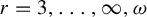 $r=3,\ldots ,\infty ,\omega $
, have a bi-focus periodic orbit
$r=3,\ldots ,\infty ,\omega $
, have a bi-focus periodic orbit
 $L_{f_0}$
whose stable and unstable manifolds
$L_{f_0}$
whose stable and unstable manifolds
 $W^s(L_{f_0})$
and
$W^s(L_{f_0})$
and
 $W^u(L_{f_0})$
contain two orbits
$W^u(L_{f_0})$
contain two orbits
 $\Gamma ^1$
,
$\Gamma ^1$
,
 $\Gamma ^2$
of corank-2 homoclinic tangency satisfying conditions (C1) and (C2). Let these tangencies be of index
$\Gamma ^2$
of corank-2 homoclinic tangency satisfying conditions (C1) and (C2). Let these tangencies be of index
 $(n,m)$
, where
$(n,m)$
, where
 $1\le n\le r-2$
and
$1\le n\le r-2$
and
 $0\le m\le n+1$
. Let the map
$0\le m\le n+1$
. Let the map
 $f_0$
be included in a finite-parameter
$f_0$
be included in a finite-parameter
 $C^r$
family of maps
$C^r$
family of maps
 $f_{\varepsilon }$
, which is proper for the global maps
$f_{\varepsilon }$
, which is proper for the global maps
 $T_{\Gamma ^1}$
,
$T_{\Gamma ^1}$
,
 $T_{\Gamma ^2}$
. Then, there exists arbitrarily small
$T_{\Gamma ^2}$
. Then, there exists arbitrarily small
 $\varepsilon ^{*}$
such that
$\varepsilon ^{*}$
such that
 $W^s(L_{f_{\varepsilon ^{*}}})$
and
$W^s(L_{f_{\varepsilon ^{*}}})$
and
 $W^u(L_{f_{\varepsilon ^{*}}})$
contain an orbit
$W^u(L_{f_{\varepsilon ^{*}}})$
contain an orbit
 $\Gamma $
of corank-2 homoclinic tangency of index not lower than
$\Gamma $
of corank-2 homoclinic tangency of index not lower than
 $(n,m+1)$
 $\text {if } 0\le m\le n$
, or
$\text {if } 0\le m\le n$
, or
 $(n+1,0)$
 $\text {if } m=n+1$
.
$\text {if } m=n+1$
.
Proof. Let
 $O_{f_0}$
be an arbitrary point from the orbit
$O_{f_0}$
be an arbitrary point from the orbit
 $L_{f_0}$
and let the corresponding local map
$L_{f_0}$
and let the corresponding local map
 $T_0$
be written in the main normal form. Similar to what we did in §3.2, we fix the points
$T_0$
be written in the main normal form. Similar to what we did in §3.2, we fix the points
 $M^+=(x^+,0,u^+,0)$
,
$M^+=(x^+,0,u^+,0)$
,
 $\hat M^+=(\hat x^+,0,\hat u^+,0)$
on
$\hat M^+=(\hat x^+,0,\hat u^+,0)$
on
 $W^s_{\mathrm {loc}}(O_{f_0})$
and
$W^s_{\mathrm {loc}}(O_{f_0})$
and
 ${M^-=(0,y^-,0, v^-)}$
,
${M^-=(0,y^-,0, v^-)}$
,
 $\hat M^-=(0,\hat y^-,0,\hat v^-)$
on
$\hat M^-=(0,\hat y^-,0,\hat v^-)$
on
 $W^u_{\mathrm {loc}}(O_{f_0})$
, where
$W^u_{\mathrm {loc}}(O_{f_0})$
, where
 $M^+, M^-$
belong to the orbit
$M^+, M^-$
belong to the orbit
 $\Gamma ^1$
and
$\Gamma ^1$
and
 $\hat M^+, \hat M^-$
belong to the orbit
$\hat M^+, \hat M^-$
belong to the orbit
 $\Gamma ^2$
. Also, we fix some small neighbourhoods
$\Gamma ^2$
. Also, we fix some small neighbourhoods
 $\Pi ^+, \Pi ^-,\hat \Pi ^+, \hat \Pi ^-$
of the points
$\Pi ^+, \Pi ^-,\hat \Pi ^+, \hat \Pi ^-$
of the points
 $M^+, M^-,\hat M^+, \hat M^-$
, respectively. Then, the global maps
$M^+, M^-,\hat M^+, \hat M^-$
, respectively. Then, the global maps
 $T_{\Gamma ^1}:\Pi ^-\rightarrow \Pi ^+$
 $(\text {with}\ T_{\Gamma ^1}:(x,y,u,v)\mapsto (\overline x,\overline y,\overline u,\overline v))$
and
$(\text {with}\ T_{\Gamma ^1}:(x,y,u,v)\mapsto (\overline x,\overline y,\overline u,\overline v))$
and
 $T_{\Gamma ^2}:\hat \Pi ^-\rightarrow \hat \Pi ^+$
 $(\text {with}\ T_{\Gamma ^2}:(\overline {\overline x},\overline {\overline y},\overline {\overline u},\overline {\overline v})\mapsto (\overline {\overline {\overline x}},\overline {\overline {\overline y}},\overline {\overline {\overline u}},\overline {\overline {\overline v}}))$
for the orbits
$(\text {with}\ T_{\Gamma ^2}:(\overline {\overline x},\overline {\overline y},\overline {\overline u},\overline {\overline v})\mapsto (\overline {\overline {\overline x}},\overline {\overline {\overline y}},\overline {\overline {\overline u}},\overline {\overline {\overline v}}))$
for the orbits
 $\Gamma ^1$
,
$\Gamma ^1$
,
 $\Gamma ^2$
, respectively, are correctly defined. The image
$\Gamma ^2$
, respectively, are correctly defined. The image
 $(\overline {\overline x},\overline {\overline y},\overline {\overline u},\overline {\overline v})=T_0^k(\overline x,\overline y,\overline u,\overline v)$
belongs to the neighbourhood
$(\overline {\overline x},\overline {\overline y},\overline {\overline u},\overline {\overline v})=T_0^k(\overline x,\overline y,\overline u,\overline v)$
belongs to the neighbourhood
 $\hat \Pi ^-$
if and only if the relations of the form in equation (19) hold.
$\hat \Pi ^-$
if and only if the relations of the form in equation (19) hold.
Let us consider the parametric family
 $f_{\varepsilon }$
. This family is proper for the orbits
$f_{\varepsilon }$
. This family is proper for the orbits
 $\Gamma ^1$
and
$\Gamma ^1$
and
 $\Gamma ^2$
, so
$\Gamma ^2$
, so
 $$ \begin{align} \text{rank }\frac{\partial(\overline\mu_{(n,m)},\overline\nu_{(n,m)},\varphi,\psi)}{\partial\varepsilon}\bigg|_{\varepsilon=0}=\chi_1(\overline\mu_{(n,m)})+\chi_2(\overline\nu_{(n,m)})+2, \end{align} $$
where
 $\overline \mu _{(n,m)}$
and
$\overline \mu _{(n,m)}$
and
 $\overline \nu _{(n,m)}$
are vectors of the splitting coefficients for the global maps
$\overline \nu _{(n,m)}$
are vectors of the splitting coefficients for the global maps
 $T_{\Gamma ^1}$
and
$T_{\Gamma ^1}$
and
 $T_{\Gamma ^2}$
, respectively, and
$T_{\Gamma ^2}$
, respectively, and
 $\varphi , \psi $
are arguments of the leading multipliers of
$\varphi , \psi $
are arguments of the leading multipliers of
 $L_{f_{\varepsilon }}$
. By equation (28), we can choose these splitting coefficients and arguments
$L_{f_{\varepsilon }}$
. By equation (28), we can choose these splitting coefficients and arguments
 $\varphi , \psi $
as the new independent parameters. Thus, we will consider a parametric family
$\varphi , \psi $
as the new independent parameters. Thus, we will consider a parametric family
 $f_{\varepsilon }$
, where
$f_{\varepsilon }$
, where
 $\varepsilon =(\overline \mu _{(n,m)},\overline \nu _{(n,m)},\varphi ,\psi )$
. For all small
$\varepsilon =(\overline \mu _{(n,m)},\overline \nu _{(n,m)},\varphi ,\psi )$
. For all small
 $\varepsilon $
, the global maps
$\varepsilon $
, the global maps
 $T_{\Gamma ^1}$
,
$T_{\Gamma ^1}$
,
 $T_{\Gamma ^2}$
can be written as
$T_{\Gamma ^2}$
can be written as
 $$ \begin{align} T_{\Gamma^1}: \;\;\; \begin{aligned} &\!\!\!\!\!\!\!\overline x_1 -x_1^+ = a_{11}x_1+a_{12}x_2+b_{11}Y_1+b_{12}Y_2+c_{1} u+d_{1} \overline v+O((x,Y,u,\overline v)^2), \\ &\!\!\!\!\!\!\!\overline x_2 -x_2^+ = a_{21}x_1+a_{22}x_2+b_{21}Y_1+b_{22}Y_2+c_{2} u+d_{2} \overline v+O((x,Y,u,\overline v)^2), \\ &\!\!\!\!\!\!\!\overline y_1 = a_{31} x_1+a_{32} x_2+\sum\limits_{j=0}^n\sum\limits_{i=0}^{j} \mu_{1,j,i}Y_1^{j-i} Y_2^{i}+\sum\limits_{i=0}^{m-1}\mu_{1,n+1,i} Y_1^{n+1-i}Y_2^{i}\\[-3pt] &\!\!\!\!\!\!\!\qquad+\sum\limits_{i=m}^{n+1}A_{1,i} Y_1^{n+1-i}Y_2^{i}+c_{3} u+d_{3} \overline v+O((x,u,\overline v)^2+\|Y\|\cdot\|x,u,\overline v\|+\|Y\|^{n+2}), \\[-3pt] &\!\!\!\!\!\!\!\overline y_2=a_{41} x_1+a_{42} x_2+\sum\limits_{j=0}^n\sum\limits_{i=0}^{j} \mu_{2,j,i} Y_1^{j-i} Y_2^{i}+\sum\limits_{i=0}^{m-1}\mu_{2,n+1,i} Y_1^{n+1-i}Y_2^{i}\\ &\!\!\!\!\!\!\!\qquad+\sum\limits_{i=m}^{n+1}A_{2,i} Y_1^{n+1-i}Y_2^{i}+c_{4} u+d_{4} \overline v+O((x,u,\overline v)^2+\|Y\|\cdot\|x,u,\overline v\|+\|Y\|^{n+2}), \\ &\!\!\!\!\!\!\!\overline u-u^+= a_{51} x_1+a_{52} x_2 + b_{51}Y_1+b_{52}Y_2+c_5 u+d_5\overline v+O((x,Y,u,\overline v)^2),\\ &\!\!\!\!\!\!\!v-v^-=a_{61} x_1+a_{62} x_2 + b_{61}Y_1+b_{62}Y_2+c_6 u+d_6\overline v+O((x,Y,u,\overline v)^2),\\ \end{aligned} \end{align} $$
and
 $$ \begin{align} &\!\!\!\!\!\!\!\overline{\overline{\overline x}}_1 -\hat x_1^+ = \hat a_{11}\overline{\overline x}_1+\hat a_{12}\overline{\overline x}_2+\hat b_{11}\overline{\overline Y}_1+\hat b_{12}\overline{\overline Y}_2+\hat c_{1} \overline{\overline u}+\hat d_{1} \overline{\overline{\overline v}}+O((\overline{\overline x},\overline{\overline Y},\overline{\overline u},\overline{\overline{\overline v}})^2), \nonumber\\ &\!\!\!\!\!\!\!\overline{\overline{\overline x}}_2 -\hat x_2^+ = \hat a_{21}\overline{\overline x}_1+\hat a_{22}\overline{\overline x}_2+\hat b_{21}\overline{\overline Y}_1+\hat b_{22}\overline{\overline Y}_2+\hat c_{2} \overline{\overline u}+\hat d_{2} \overline{\overline{\overline v}}+O((\overline{\overline x},\overline{\overline Y},\overline{\overline u},\overline{\overline{\overline v}})^2), \nonumber\\ &\!\!\!\!\!\!\!\overline{\overline{\overline y}}_1 = \hat a_{31} \overline{\overline x}_1+\hat a_{32} \overline{\overline x}_2+\sum\limits_{j=0}^n\sum\limits_{i=0}^{j} \nu_{1,j,i}\overline{\overline Y}_1^{\,j-i} \,\overline{\overline Y}_2^{\, i}+\sum\limits_{i=0}^{m-1}\nu_{1,n+1,i} \overline{\overline Y}_1^{\,n+1-i}\,\overline{\overline Y}_2^{\,i}\nonumber\\ &\!\!\!\!\!\!\!\qquad+\hspace{-1pt}\sum\limits_{i=m}^{n+1}B_{1,i} \overline{\overline Y}_1^{\,n+1-i}\,\overline{\overline Y}_2^{\,i}\hspace{-0.5pt}+\hspace{-0.5pt}\hat c_{3} \overline{\overline u}+\hat d_{3} \overline{\overline{\overline v}}\hspace{-0.5pt}+\hspace{-0.5pt}O((\overline{\overline x},\overline{\overline u}, \overline{\overline{\overline v}})^2+\|\overline{\overline Y}\|\cdot\|\overline{\overline x},\overline{\overline u}, \overline{\overline{\overline v}}\|\hspace{-0.5pt}+\hspace{-0.5pt}\|\overline{\overline Y}\|^{n+2}), \nonumber T_{\Gamma^2}: \;\;\;\nonumber\\&\!\!\!\!\!\!\!\overline{\overline{\overline y}}_2=\hat a_{41} \overline{\overline x}_1+\hat a_{42} \overline{\overline x}_2+\sum\limits_{j=0}^n\sum\limits_{i=0}^{j} \nu_{2,j,i} \overline{\overline Y}_1^{\,j-i} \,\overline{\overline Y}_2^{\,i}+\sum\limits_{i=0}^{m-1}\nu_{2,n+1,i} \overline{\overline Y}_1^{\,n+1-i}\,\overline{\overline Y}_2^{\,i}\nonumber\\ &\!\!\!\!\!\!\!\qquad+\hspace{-0.5pt}\sum\limits_{i=m}^{n+1}B_{2,i} \overline{\overline Y}_1^{\,n+1-i}\,\overline{\overline Y}_2^{\,i}\hspace{-0.5pt}+\hspace{-0.5pt}\hat c_{4} \overline{\overline u}+\hat d_{4} \overline{\overline{\overline v}}\hspace{-0.5pt}+\hspace{-0.5pt}O((\overline{\overline x},\overline{\overline u}, \overline{\overline{\overline v}})^2+\|\overline{\overline Y}\|\cdot\|\overline{\overline x},\overline{\overline u}, \overline{\overline{\overline v}}\|+\|\overline{\overline Y}\|^{n+2}), \nonumber\\ &\!\!\!\!\!\!\!\overline{\overline{\overline u}}-\hat u^+= \hat a_{51} \overline{\overline x}_1+\hat a_{52} \overline{\overline x}_2 + \hat b_{51}\overline{\overline Y}_1+\hat b_{52}\overline{\overline Y}_2+\hat c_5 \overline{\overline u}+\hat d_5\overline{\overline{\overline v}}+O((\overline{\overline x},\overline{\overline Y},\overline{\overline u},\overline{\overline{\overline v}})^2),\nonumber\\ &\!\!\!\!\!\!\!\overline{\overline v}-\hat v^-=\hat a_{61} \overline{\overline x}_1+\hat a_{62} \overline{\overline x}_2 + \hat b_{61}\overline{\overline Y}_1+\hat b_{62}\overline{\overline Y}_2+\hat c_6 \overline{\overline u}+\hat d_6\overline{\overline{\overline v}}+O((\overline{\overline x},\overline{\overline Y},\overline{\overline u},\overline{\overline{\overline v}})^2),\nonumber\\ \end{align} $$
where
 $Y=y-y^-$
and
$Y=y-y^-$
and
 $\overline {\overline Y}=\overline {\overline y}-\hat y^-$
. By Proposition 3.1, the equations for the iterations
$\overline {\overline Y}=\overline {\overline y}-\hat y^-$
. By Proposition 3.1, the equations for the iterations
 $T_0^k$
of the local map have the following form (in formulae for y-coordinates, we expressed
$T_0^k$
of the local map have the following form (in formulae for y-coordinates, we expressed
 $\overline {\overline y}_{1}$
,
$\overline {\overline y}_{1}$
,
 $\overline {\overline y}_{2}$
in terms of
$\overline {\overline y}_{2}$
in terms of
 $\overline y_1$
,
$\overline y_1$
,
 $\overline y_2$
in the linear part):
$\overline y_2$
in the linear part):

We will consider a global map
 $T_{\Gamma }:\Pi ^-\rightarrow \hat \Pi ^+$
such that
$T_{\Gamma }:\Pi ^-\rightarrow \hat \Pi ^+$
such that
 $T_{\Gamma }= T_{\Gamma ^2}\circ T_0^k\circ T_{\Gamma ^1}$
(see Figure 4) and show that there exists a sequence
$T_{\Gamma }= T_{\Gamma ^2}\circ T_0^k\circ T_{\Gamma ^1}$
(see Figure 4) and show that there exists a sequence
 $(k_{\alpha })_{\alpha \in \mathbb N}$
with the following property:
$(k_{\alpha })_{\alpha \in \mathbb N}$
with the following property:
 $k_{\alpha }\xrightarrow [\alpha \rightarrow +\infty ]{}+\infty $
and for each
$k_{\alpha }\xrightarrow [\alpha \rightarrow +\infty ]{}+\infty $
and for each
 $\alpha $
, the parameters
$\alpha $
, the parameters
 $\mu $
and
$\mu $
and
 $\nu $
can be chosen in such a way that the map
$\nu $
can be chosen in such a way that the map
 $T_{\Gamma }$
corresponds to an orbit
$T_{\Gamma }$
corresponds to an orbit
 $\Gamma $
of corank-2 homoclinic tangency of index not lower than
$\Gamma $
of corank-2 homoclinic tangency of index not lower than
 $(n,m+1)$
 $\text {if } 0\le m\le n$
, or
$\text {if } 0\le m\le n$
, or
 $(n+1,0)$
 $\text {if } m=n+1$
. In addition, the values of these parameters tend to zero as
$\text {if } m=n+1$
. In addition, the values of these parameters tend to zero as
 $\alpha \rightarrow +\infty $
. For this purpose, it is enough to consider only the third and the fourth lines in equation (30). Also, to simplify computations, we put
$\alpha \rightarrow +\infty $
. For this purpose, it is enough to consider only the third and the fourth lines in equation (30). Also, to simplify computations, we put
 $x_1,x_2,u,\overline {\overline {\overline v}}$
equal to zero, so we consider the restriction
$x_1,x_2,u,\overline {\overline {\overline v}}$
equal to zero, so we consider the restriction
 $T_{\Gamma }|_{(Y_1,Y_2)}$
.
$T_{\Gamma }|_{(Y_1,Y_2)}$
.
The global map
 $T_{\Gamma }:\Pi ^-\rightarrow \Pi ^+$
is given by the composition
$T_{\Gamma }:\Pi ^-\rightarrow \Pi ^+$
is given by the composition
 $T_{\Gamma }= T_{\Gamma ^2}\circ T_0^k\circ T_{\Gamma ^1}$
, where
$T_{\Gamma }= T_{\Gamma ^2}\circ T_0^k\circ T_{\Gamma ^1}$
, where
 $T_0$
is the local map near the periodic point
$T_0$
is the local map near the periodic point
 $O_{f_{\varepsilon }}$
and
$O_{f_{\varepsilon }}$
and
 $T_{\Gamma ^1}:\Pi ^-\rightarrow \Pi ^+$
,
$T_{\Gamma ^1}:\Pi ^-\rightarrow \Pi ^+$
,
 $T_{\Gamma ^2}:\hat \Pi ^-\rightarrow \hat \Pi ^+$
are the global maps for the orbits
$T_{\Gamma ^2}:\hat \Pi ^-\rightarrow \hat \Pi ^+$
are the global maps for the orbits
 $\Gamma ^1$
,
$\Gamma ^1$
,
 $\Gamma ^2$
, respectively.
$\Gamma ^2$
, respectively.

We start with the consideration of the composition
 $T_0^k \circ T_{\Gamma ^1}|_{(Y_1,Y_2)}$
. Combining equations (29) and (31), we get
$T_0^k \circ T_{\Gamma ^1}|_{(Y_1,Y_2)}$
. Combining equations (29) and (31), we get

where
 $$ \begin{align*} \begin{aligned} &\tilde x^+_{1}=x^+_{1}\cos(k\varphi)-x^+_{2}\sin(k\varphi), \tilde x^+_{2}=x^+_{1}\sin(k\varphi)+x^+_{2}\cos(k\varphi),\\ \end{aligned} \end{align*} $$
and for
 $i\in \{1,2\}$
, one has
$i\in \{1,2\}$
, one has
 $$ \begin{align*} \begin{aligned} &\tilde b_{1i}=b_{1i}\cos(k\varphi)-b_{2i}\sin(k\varphi), \tilde b_{2i}=b_{1i}\sin(k\varphi)+b_{2i}\cos(k\varphi),\\ \end{aligned} \end{align*} $$
for
 $0\le j\le n$
,
$0\le j\le n$
,
 $0\le i\le j$
and
$0\le i\le j$
and
 $j=n+1$
,
$j=n+1$
,
 $0\le i\le m-1$
, one has
$0\le i\le m-1$
, one has
 $$ \begin{align*} \begin{aligned} &\tilde{\mu}_{1,j,i}=\mu_{1,j,i}\cos(k\psi)-\mu_{2,j,i}\sin(k\psi), \tilde{\mu}_{2,j,i}=\mu_{1,j,i}\sin(k\psi)+\mu_{2,j,i}\cos(k\psi),\\ \end{aligned} \end{align*} $$
and for
 $i\in \{m,\ldots ,n+1\}$
, one has
$i\in \{m,\ldots ,n+1\}$
, one has
 $$ \begin{align} \begin{aligned} &\tilde A_{1,i}=A_{1,i}\cos(k\psi)-A_{2,i}\sin(k\psi), \tilde A_{2,i}=A_{1,i}\sin(k\psi)+A_{2,i}\cos(k\psi).\\ \end{aligned} \end{align} $$
Let us make the following change of parameters:
 $$ \begin{align} \begin{aligned} \dot\mu_{1,j,i}&=\tilde{\mu}_{1,j,i}\hspace{-0.5pt}+\hspace{-0.5pt}O(\hat\gamma^{-k}) \quad\text{and}\quad \dot\mu_{2,j,i}\hspace{-0.5pt}=\hspace{-0.5pt}\tilde{\mu}_{2,j,i}\hspace{-0.5pt}+\hspace{-0.5pt}O(\hat\gamma^{-k})\quad \text{for } 0\hspace{-0.5pt}\le\hspace{-0.5pt} j\hspace{-0.5pt}\le\hspace{-0.5pt} n, 0\le i\le j,\\ \dot\mu_{1,n+1,i}&=\tilde{\mu}_{1,n+1,i}\hspace{-0.5pt}+\hspace{-0.5pt}O(\hat\gamma^{-k}) \quad\text{and}\quad \dot\mu_{2,n+1,i}\hspace{-0.5pt}=\hspace{-0.5pt}\tilde{\mu}_{2,n+1,i}\hspace{-0.5pt}+\hspace{-0.5pt}O(\hat\gamma^{-k})\quad \text{for } 0\hspace{-0.5pt}\le\hspace{-0.5pt} i\hspace{-0.5pt}\le\hspace{-0.5pt} m-1, \end{aligned} \end{align} $$
to get rid of the corresponding small terms (of order
 $O(\gamma ^k\hat \gamma ^{-k})$
) in the third and the fourth lines in equation (32).
$O(\gamma ^k\hat \gamma ^{-k})$
) in the third and the fourth lines in equation (32).
Now, we start choosing the parameters
 $\dot \mu $
and
$\dot \mu $
and
 $\nu $
to obtain the sought tangency. Let us put
$\nu $
to obtain the sought tangency. Let us put
 $$ \begin{align} \begin{aligned} &\dot\mu_{1,0,0}=\gamma^{-k}\cdot\hat y_1^{-},\quad \dot\mu_{2,0,0}=\gamma^{-k}\cdot\hat y_2^{-},\quad \dot\mu_{1,1,1}=0,\quad \dot\mu_{2,1,0}=0.\\ \end{aligned} \end{align} $$
In equation (30) for the map
 $T_{\Gamma ^2}$
, let us put
$T_{\Gamma ^2}$
, let us put
 $$ \begin{align} \begin{aligned} \nu_{1,j,i}&=0 \quad\text{and}\quad \nu_{2,j,i}=0\quad \text{for } 2\le j\le n, 0\le i\le j,\\ \nu_{1,n+1,i}&=0 \quad\text{and}\quad \nu_{2,n+1,i}=0\quad \text{for } 0\le i\le m-1. \end{aligned} \end{align} $$
Next, we consider the composition
 $T_{\Gamma }|_{(Y_1,Y_2)}=T_{\Gamma ^2}\circ T_0^{k}\circ T_{\Gamma ^1}|_{(Y_1,Y_2)}$
taking into account equations (34), (35) and (36). As we have already mentioned, we will write just the third and the fourth lines (for
$T_{\Gamma }|_{(Y_1,Y_2)}=T_{\Gamma ^2}\circ T_0^{k}\circ T_{\Gamma ^1}|_{(Y_1,Y_2)}$
taking into account equations (34), (35) and (36). As we have already mentioned, we will write just the third and the fourth lines (for
 $\overline {\overline {\overline y}}_1$
and
$\overline {\overline {\overline y}}_1$
and
 $\overline {\overline {\overline y}}_2$
). The equation for
$\overline {\overline {\overline y}}_2$
). The equation for
 $\overline {\overline {\overline y}}_1$
has the form
$\overline {\overline {\overline y}}_1$
has the form
 $$ \begin{align*} \begin{aligned} \overline{\overline{\overline y}}_1&=\unicode{x3bb}^k\cdot\hat a_{31}(\tilde x_1^++\tilde b_{11}Y_1+\tilde b_{12}Y_2+O(Y^2))\\&\quad+\unicode{x3bb}^k\cdot\hat a_{32}(\tilde x_2^++\tilde b_{21}Y_1+\tilde b_{22}Y_2+O(Y^2))+\nu_{1,0,0}\\ &\quad+\gamma^k\cdot \nu_{1,1,0}\bigg(\dot\mu_{1,1,0}Y_1+\sum\limits_{j=2}^n\sum\limits_{i=0}^{j} \dot\mu_{1,j,i}Y_1^{j-i} Y_2^{i}+\sum\limits_{i=0}^{m-1}\dot\mu_{1,n+1,i}Y_1^{n+1-i}Y_2^{i} \\&\quad +\sum\limits_{i=m}^{n+1}\tilde A_{1,i} Y_1^{n+1-i}Y_2^{i}+O(\hat\gamma^{-k})\bigg)+\gamma^k\cdot \nu_{1,1,1}\bigg(\dot\mu_{2,1,1}Y_2+\sum\limits_{j=2}^n\sum\limits_{i=0}^{j} \dot \mu_{2,j,i} Y_1^{j-i} Y_2^{i}\\ &\quad+\sum\limits_{i=0}^{m-1}\dot\mu_{2,n+1,i} Y_1^{n+1-i}Y_2^{i}+\sum\limits_{i=m}^{n+1}\tilde A_{2,i} Y_1^{n+1-i}Y_2^{i}+O(\hat\gamma^{-k})\bigg)\\ &\quad+\gamma^{k(n+1)}\cdot\sum\limits_{t=m}^{n+1}B_{1,t} \bigg(\dot\mu_{1,1,0}Y_1+\sum\limits_{j=2}^n\sum\limits_{i=0}^{j} \dot\mu_{1,j,i}Y_1^{j-i} Y_2^{i}+\sum\limits_{i=0}^{m-1}\dot\mu_{1,n+1,i} Y_1^{n+1-i}Y_2^{i}\\ &\quad+\sum\limits_{i=m}^{n+1}\tilde A_{1,i} Y_1^{n+1-i}Y_2^{i}+O(\hat\gamma^{-k})\bigg)^{n+1-t}\times \bigg(\dot\mu_{2,1,1}Y_2+\sum\limits_{j=2}^n\sum\limits_{i=0}^{j} \dot \mu_{2,j,i} Y_1^{j-i} Y_2^{i}\\&\quad+\sum\limits_{i=0}^{m-1}\dot\mu_{2,n+1,i} Y_1^{n+1-i}Y_2^{i}+\sum\limits_{i=m}^{n+1}\tilde A_{2,i} Y_1^{n+1-i}Y_2^{i}+O(\hat\gamma^{-k})\bigg)^{t}+O(\|Y\|^{n+2})+o(\unicode{x3bb}^k), \end{aligned} \end{align*} $$
while the equation for
 $\overline {\overline {\overline y}}_2$
is given by
$\overline {\overline {\overline y}}_2$
is given by
 $$ \begin{align*} \begin{aligned} \overline{\overline{\overline y}}_2&=\unicode{x3bb}^k\cdot\hat a_{41}(\tilde x_1^++\tilde b_{11}Y_1+\tilde b_{12}Y_2+O(Y^2))\\&\quad+\unicode{x3bb}^k\cdot\hat a_{42}(\tilde x_2^++\tilde b_{21}Y_1+\tilde b_{22}Y_2+O(Y^2))+\nu_{2,0,0}\\[-3pt] &\quad+\gamma^k\cdot \nu_{2,1,0}\bigg(\dot\mu_{1,1,0}Y_1+\sum\limits_{j=2}^n\sum\limits_{i=0}^{j} \dot\mu_{1,j,i}Y_1^{j-i} Y_2^{i}+\sum\limits_{i=0}^{m-1}\dot\mu_{1,n+1,i} Y_1^{n+1-i}Y_2^{i}\\[-3pt] &\quad +\sum\limits_{i=m}^{n+1}\tilde A_{1,i} Y_1^{n+1-i}Y_2^{i}+O(\hat\gamma^{-k})\bigg) +\gamma^k\cdot \nu_{2,1,1}\bigg(\dot\mu_{2,1,1}Y_2+\sum\limits_{j=2}^n\sum\limits_{i=0}^{j} \dot \mu_{2,j,i} Y_1^{j-i} Y_2^{i}\\[-3pt] &\quad +\sum\limits_{i=0}^{m-1}\dot\mu_{2,n+1,i} Y_1^{n+1-i}Y_2^{i} +\sum\limits_{i=m}^{n+1}\tilde A_{2,i} Y_1^{n+1-i}Y_2^{i}+O(\hat\gamma^{-k})\bigg)\\[-3pt] &\quad+\gamma^{k(n+1)}\cdot\sum\limits_{t=m}^{n+1}B_{2,t} \bigg(\dot\mu_{1,1,0}Y_1+\sum\limits_{j=2}^n\sum\limits_{i=0}^{j} \dot\mu_{1,j,i}Y_1^{j-i} Y_2^{i} +\sum\limits_{i=0}^{m-1}\dot\mu_{1,n+1,i} Y_1^{n+1-i}Y_2^{i}\\[-3pt] &\quad+\hspace{-0.5pt}\sum\limits_{i=m}^{n+1}\tilde A_{1,i} Y_1^{n+1-i}Y_2^{i}\hspace{-1pt}+\hspace{-1pt}O(\hat\gamma^{-k})\bigg)^{n+1-t}\kern1pt{\times} \bigg(\kern-1.3pt\dot\mu_{2,1,1}Y_2\kern1pt{+}\hspace{-1pt}\kern1pt\sum\limits_{j=2}^n\sum\limits_{i=0}^{j} \dot \mu_{2,j,i} Y_1^{j-i} Y_2^{i} Y_1^{n+1-i}Y_2^{i}\\[-3pt] &\quad+\sum\limits_{i=m}^{n+1}\tilde A_{2,i} Y_1^{n+1-i}Y_2^{i}+\sum\limits_{i=0}^{m-1}\dot\mu_{2,n+1,i}+O(\hat\gamma^{-k})\bigg)^{t}+O(\|Y\|^{n+2})+o(\unicode{x3bb}^k). \end{aligned} \end{align*} $$
We have to choose the remaining parameters
 $\dot \mu $
and
$\dot \mu $
and
 $\nu $
in such a way that in the equations above, all
$\nu $
in such a way that in the equations above, all
 $Y_1, Y_2$
-terms are zero up to the index
$Y_1, Y_2$
-terms are zero up to the index
 $Y_1^{n+1-m}\cdot Y_2^m$
(including). These values of the parameters are the solutions of the system
$Y_1^{n+1-m}\cdot Y_2^m$
(including). These values of the parameters are the solutions of the system
 $$ \begin{align} \begin{aligned} &\gamma^{k(n+1)}\cdot\dot\mu_{1,1,0}^{n+1-m}\cdot\dot\mu_{2,1,1}^m\cdot B_{1,m}+\gamma^k\cdot \nu_{1,1,0}\cdot(\tilde A_{1,m}+O(\hat\gamma^{-k}))\\&\quad+\gamma^k \cdot \nu_{1,1,1}\cdot(\tilde A_{2,m}+O(\hat\gamma^{-k}))=O(\unicode{x3bb}^k),\\ &\gamma^{k(n+1)}\cdot\dot\mu_{1,1,0}^{n+1-m}\cdot\dot\mu_{2,1,1}^m\cdot B_{2,m}+\gamma^k\cdot \nu_{2,1,0}\cdot(\tilde A_{1,m}+O(\hat\gamma^{-k}))\\&\quad+\gamma^k \cdot \nu_{2,1,1}\cdot(\tilde A_{2,m}+O(\hat\gamma^{-k}))=O(\unicode{x3bb}^k),\\ &\nu_{1,0,0}=O(\unicode{x3bb}^k),\quad \nu_{2,0,0}=O(\unicode{x3bb}^k),\\ &\gamma^k\cdot \nu_{1,1,0}\cdot\dot\mu_{1,1,0}=\unicode{x3bb}^k\cdot S_{1}+o(\unicode{x3bb}^k),\quad \gamma^k\cdot \nu_{2,1,0}\cdot\dot\mu_{1,1,0}=\unicode{x3bb}^k \cdot S_{3}+o(\unicode{x3bb}^k),\\ &\gamma^k\cdot \nu_{1,1,1}\cdot\dot\mu_{2,1,1}=\unicode{x3bb}^k\cdot S_{2}+o(\unicode{x3bb}^k),\quad \gamma^k\cdot \nu_{2,1,1}\cdot\dot\mu_{2,1,1}=\unicode{x3bb}^k \cdot S_{4}+o(\unicode{x3bb}^k),\\ &\gamma^k\hspace{-0.5pt}\cdot\hspace{-0.5pt}(\nu_{1,1,0}\hspace{-0.5pt}\cdot\hspace{-0.5pt}\dot\mu_{1,j,i}\hspace{-0.5pt}+\hspace{-0.5pt}\nu_{1,1,1}\cdot\dot\mu_{2,j,i})\hspace{-0.5pt}=\hspace{-0.5pt}O(\unicode{x3bb}^k),\ \gamma^k\hspace{-0.5pt}\cdot\hspace{-0.5pt}(\nu_{2,1,0}\cdot\dot\mu_{1,j,i}+\nu_{2,1,1}\cdot\dot\mu_{2,j,i})=O(\unicode{x3bb}^k), \end{aligned} \end{align} $$
where
 $2\le j\le n, 0\le i\le j$
and
$2\le j\le n, 0\le i\le j$
and
 $j=n+1, 0\le i\le m-1$
, and where
$j=n+1, 0\le i\le m-1$
, and where
 $S_1,S_2,S_3,S_4$
are given by
$S_1,S_2,S_3,S_4$
are given by
 $$ \begin{align} \begin{aligned} S_1&= \hat a_{31}\tilde b_{11}+\hat a_{32}\tilde b_{21}=\hat a_{31}(b_{11}\cos(k\varphi)-b_{21}\sin(k\varphi))+\hat a_{32}(b_{11}\sin(k\varphi)+b_{21}\cos(k\varphi)),\\ S_2&= \hat a_{31}\tilde b_{12}+\hat a_{32}\tilde b_{22}=\hat a_{31}(b_{12}\cos(k\varphi)-b_{22}\sin(k\varphi))+\hat a_{32}(b_{12}\sin(k\varphi)+b_{22}\cos(k\varphi)),\\ S_3&= \hat a_{41}\tilde b_{11}+\hat a_{42}\tilde b_{21}=\hat a_{41}(b_{11}\cos(k\varphi)-b_{21}\sin(k\varphi))+\hat a_{42}(b_{11}\sin(k\varphi)+b_{21}\cos(k\varphi)),\\ S_4&= \hat a_{41}\tilde b_{12}+\hat a_{42}\tilde b_{22}=\hat a_{41}(b_{12}\cos(k\varphi)-b_{22}\sin(k\varphi))+\hat a_{42}(b_{12}\sin(k\varphi)+b_{22}\cos(k\varphi)).\\ \end{aligned} \end{align} $$
Let us make a rescaling of the parameters
 $$ \begin{align} \begin{aligned} M_{1,1,0}&=\unicode{x3bb}^{-{k}/({n+2})}\cdot\gamma^{{k(n+1)}/({n+2})}\cdot\dot\mu_{1,1,0}, \quad &M_{2,1,1}&=\unicode{x3bb}^{-{k}/({n+2})}\cdot\gamma^{{k(n+1)}/({n+2})}\cdot\dot\mu_{2,1,1},\\ M_{1,j,i}&=\unicode{x3bb}^{-{k}/({n+2})}\cdot\gamma^{{k(n+1)}/({n+2})}\cdot\dot\mu_{1,j,i}, \quad &M_{2,j,i}&=\unicode{x3bb}^{-{k}/({n+2})}\cdot\gamma^{{k(n+1)}/({n+2})}\cdot\dot\mu_{2,j,i},\\ N_{1,0,0}&=\unicode{x3bb}^{-k}\cdot \nu_{1,0,0}, \quad &N_{2,0,0}&=\unicode{x3bb}^{-k}\cdot \nu_{2,0,0},\\ N_{1,1,0}&=\unicode{x3bb}^{{k(n+1)}/({n+2})}\cdot\gamma^{{k}/({n+2})}\cdot \nu_{1,1,0}, \quad &N_{2,1,0}&=\unicode{x3bb}^{{k(n+1)}/({n+2})}\cdot\gamma^{{k}/({n+2})}\cdot \nu_{2,1,0},\\ N_{1,1,1}&=\unicode{x3bb}^{{k(n+1)}/({n+2})}\cdot\gamma^{{k}/({n+2})}\cdot \nu_{1,1,1}, \quad &N_{2,1,1}&=\unicode{x3bb}^{{k(n+1)}/({n+2})}\cdot\gamma^{{k}/({n+2})}\cdot \nu_{2,1,1}.\\ \end{aligned} \end{align} $$
After it, the system of equation (37) recasts as
 $$ \begin{align} \begin{aligned} &M_{1,1,0}^{n+1-m}\cdot M_{2,1,1}^m\cdot B_{1,m}+N_{1,1,0}\cdot(\tilde A_{1,m}+O(\hat\gamma^{-k}))+N_{1,1,1}\cdot(\tilde A_{2,m}+O(\hat\gamma^{-k}))\\&\quad=O(\unicode{x3bb}^{{k}/({n+2})}\cdot\gamma^{-{k(n+1)}/({n+2})}),\\ &M_{1,1,0}^{n+1-m}\cdot M_{2,1,1}^m\cdot B_{2,m}+N_{2,1,0}\cdot(\tilde A_{1,m}+O(\hat\gamma^{-k}))+N_{2,1,1}\cdot(\tilde A_{2,m}+O(\hat\gamma^{-k}))\\&\quad=O(\unicode{x3bb}^{{k}/({n+2})}\cdot\gamma^{-{k(n+1)}/({n+2})}),\\ &N_{1,0,0}=O(1),\quad N_{2,0,0}=O(1),\\ &N_{1,1,0}\cdot M_{1,1,0}=S_{1}+o(1)_{k\to+\infty},\quad N_{2,1,0}\cdot M_{1,1,0}=S_{3}+o(1)_{k\to+\infty},\\ &N_{1,1,1}\cdot M_{2,1,1}=S_2+o(1)_{k\to+\infty},\quad N_{2,1,1}\cdot M_{2,1,1}=S_4+o(1)_{k\to+\infty},\\ &N_{1,1,0}\cdot M_{1,j,i}+N_{1,1,1}\cdot M_{2,j,i}=O(1),\quad N_{2,1,0}\cdot M_{1,j,i}+N_{2,1,1}\cdot M_{2,j,i}=O(1). \end{aligned} \end{align} $$
Next, assuming that
 $M_{1,1,0}$
and
$M_{1,1,0}$
and
 $M_{2,1,1}$
are non-zero, we rewrite the system of equation (40) as
$M_{2,1,1}$
are non-zero, we rewrite the system of equation (40) as
 $$ \begin{align} \begin{aligned} &M_{1,1,0}^{n+2-m}\cdot M_{2,1,1}^{m+1}\cdot B_{1,m}+S_1\cdot M_{2,1,1}\cdot\tilde A_{1,m}+S_2\cdot M_{1,1,0}\cdot\tilde A_{2,m}=o(1)_{k\to+\infty},\\ &M_{1,1,0}^{n+2-m}\cdot M_{2,1,1}^{m+1}\cdot B_{2,m}+S_3\cdot M_{2,1,1}\cdot\tilde A_{1,m}+S_4\cdot M_{1,1,0}\cdot\tilde A_{2,m}=o(1)_{k\to+\infty},\\ &N_{1,0,0}=O(1), N_{2,0,0}=O(1),\\ &N_{1,1,0}=\frac{S_{1}}{M_{1,1,0}}+o(1)_{k\to+\infty},\quad N_{2,1,0}=\frac{S_{3}}{M_{1,1,0}}+o(1)_{k\to+\infty},\\ &N_{1,1,1}=\frac{S_2}{M_{2,1,1}}+o(1)_{k\to+\infty},\quad N_{2,1,1}=\frac{S_4}{M_{2,1,1}}+o(1)_{k\to+\infty},\\ &S_1\cdot M_{2,1,1}\cdot M_{1,j,i}+S_2\cdot M_{1,1,0}\cdot M_{2,j,i}\\&\quad=O(1), S_3\cdot M_{2,1,1}\cdot M_{1,j,i}+S_4\cdot M_{1,1,0}\cdot M_{2,j,i}=O(1). \end{aligned} \end{align} $$
According to Lemma 3.3, we have
 $$ \begin{align} \begin{aligned} &\det \begin{pmatrix}\hat a_{31}& \hat a_{32}\\ \hat a_{41}& \hat a_{42}\end{pmatrix}\not=0 \quad \text{and} \quad \det \begin{pmatrix} b_{11}& b_{12}\\ b_{21}& b_{22}\end{pmatrix}\not=0. \end{aligned} \end{align} $$
Denote
 $S=S_1S_4-S_2S_3$
. It is directly verified that
$S=S_1S_4-S_2S_3$
. It is directly verified that
 $$ \begin{align*} \begin{aligned} &S=\det \begin{pmatrix}\hat a_{31}& \hat a_{32}\\ \hat a_{41}& \hat a_{42}\end{pmatrix}\cdot\det \begin{pmatrix} b_{11}& b_{12}\\ b_{21}& b_{22}\end{pmatrix}\not=0.\\ \end{aligned} \end{align*} $$
Considering that S,
 $M_{1,1,0}$
and
$M_{1,1,0}$
and
 $M_{2,1,1}$
are non-zero, we can immediately find the values of
$M_{2,1,1}$
are non-zero, we can immediately find the values of
 $M_{1,j,i}$
and
$M_{1,j,i}$
and
 $M_{2,j,i}$
for all
$M_{2,j,i}$
for all
 $j,i$
satisfying
$j,i$
satisfying
 $2\le j\le n, 0\le i\le j$
and
$2\le j\le n, 0\le i\le j$
and
 $j=n+1, 0\le i\le m-1$
(see equation (41)). Therefore, to solve the system in equation (41), it is enough to find non-zero
$j=n+1, 0\le i\le m-1$
(see equation (41)). Therefore, to solve the system in equation (41), it is enough to find non-zero
 $M_{1,1,0}$
and
$M_{1,1,0}$
and
 $M_{2,1,1}$
which solve the nonlinear system
$M_{2,1,1}$
which solve the nonlinear system
 $$ \begin{align} \begin{aligned} &M_{1,1,0}^{n+2-m}\cdot M_{2,1,1}^{m+1}\cdot B_{1,m}+S_1\cdot M_{2,1,1}\cdot\tilde A_{1,m}+S_2\cdot M_{1,1,0}\cdot\tilde A_{2,m}=o(1)_{k\to+\infty},\\ &M_{1,1,0}^{n+2-m}\cdot M_{2,1,1}^{m+1}\cdot B_{2,m}+S_3\cdot M_{2,1,1}\cdot\tilde A_{1,m}+S_4\cdot M_{1,1,0}\cdot\tilde A_{2,m}=o(1)_{k\to+\infty}.\\ \end{aligned} \end{align} $$
In this system, we multiply the first equation by
 $B_{2,m}$
and the second equation by
$B_{2,m}$
and the second equation by
 $B_{1,m}$
. After that, subtracting the second equation from the first one, we obtain the relation
$B_{1,m}$
. After that, subtracting the second equation from the first one, we obtain the relation
 $$ \begin{align} \begin{aligned} &\tilde A_{1,m}\cdot(S_1B_{2,m}-S_3B_{1,m})\cdot M_{2,1,1}+\tilde A_{2,m}\cdot(S_2B_{2,m}-S_4B_{1,m})\cdot M_{1,1,0}=o(1)_{k\to+\infty}. \end{aligned} \end{align} $$
Note that by virtue of equations (33) and (38), the following matrix relations hold:
 $$ \begin{align} \begin{aligned} &\begin{pmatrix} \tilde A_{1,m} \\ \tilde A_{2,m} \end{pmatrix}=\begin{pmatrix} \cos(k\psi)& -\sin(k\psi)\\ \sin(k\psi)& \cos(k\psi)\end{pmatrix}\cdot \begin{pmatrix} A_{1,m} \\ A_{2,m} \end{pmatrix} \end{aligned} \end{align} $$
and
 $$ \begin{align} &\begin{pmatrix}S_1B_{2,m}-S_3B_{1,m} \\ S_2B_{2,m}-S_4B_{1,m} \end{pmatrix}=\begin{pmatrix} S_1& S_3\\ S_2& S_4\end{pmatrix}\cdot \begin{pmatrix} B_{2,m} \notag\\ -B_{1,m} \end{pmatrix}\\ &\quad=\begin{pmatrix} b_{11}& b_{21}\\ b_{12}& b_{22}\end{pmatrix}\cdot\begin{pmatrix} \cos(k\varphi)& \sin(k\varphi)\\ -\sin(k\varphi)& \cos(k\varphi)\end{pmatrix}\cdot\begin{pmatrix}\hat a_{31}& \hat a_{41}\\ \hat a_{32}& \hat a_{42}\end{pmatrix}\cdot\begin{pmatrix} B_{2,m} \\ -B_{1,m} \end{pmatrix}. \end{align} $$
To solve the system in equation (43), we must ensure that the factors in equation (44) are non-zero and have some definite signs. We will achieve it by the choice of some special values of k. Let us slightly vary the parameters
 $\varphi $
,
$\varphi $
,
 $\psi $
to make them and
$\psi $
to make them and
 $1$
rationally independent (the numbers
$1$
rationally independent (the numbers
 $\varphi $
,
$\varphi $
,
 $\psi $
and 1 are said to be rationally independent if
$\psi $
and 1 are said to be rationally independent if
 $k_1\varphi +k_2\psi $
is not an integer for any set of integers
$k_1\varphi +k_2\psi $
is not an integer for any set of integers
 $k_1,k_2$
, except
$k_1,k_2$
, except
 $k_1=k_2=0$
). Taking into account the conditions (42) and the equations
$k_1=k_2=0$
). Taking into account the conditions (42) and the equations
 $|A_{1,m}|+|A_{2,m}|\not =0, |B_{1,m}|+|B_{2,m}|\not =0$
, it is clear from equations (45) and (46) that we can choose a sequence
$|A_{1,m}|+|A_{2,m}|\not =0, |B_{1,m}|+|B_{2,m}|\not =0$
, it is clear from equations (45) and (46) that we can choose a sequence
 $(k_{\alpha })_{\alpha \in \mathbb N}$
such that
$(k_{\alpha })_{\alpha \in \mathbb N}$
such that
 $k_{\alpha }\xrightarrow [\alpha \rightarrow +\infty ]{}+\infty $
and
$k_{\alpha }\xrightarrow [\alpha \rightarrow +\infty ]{}+\infty $
and
 $$ \begin{align} \begin{aligned} \tilde A_{1,m}&\xrightarrow[\alpha\rightarrow+\infty]{}Q_1, &\tilde A_{2,m}&\xrightarrow[\alpha\rightarrow+\infty]{}Q_2,\\ S_1B_{2,m}-S_3B_{1,m}&\xrightarrow[\alpha\rightarrow+\infty]{}Q_3, &S_2B_{2,m}-S_4B_{1,m}&\xrightarrow[\alpha\rightarrow+\infty]{}Q_4.\\ \end{aligned} \end{align} $$
Here,
 $Q_1,\ldots ,Q_4$
are non-zero constants satisfying
$Q_1,\ldots ,Q_4$
are non-zero constants satisfying
 $$ \begin{align} \begin{aligned} \text{sgn}\, Q_1&= \text{sgn}\, S, &\text{sgn}\, Q_2&= -\text{sgn}\, S, &Q_3&>0, &Q_4&>0,\\ \end{aligned} \end{align} $$
where
 $\text {sgn}\, x$
denotes the sign function. Now, making use of equation (44) and conditions (47) and (48), we can easily find non-zero solution of the system in equation (43). This solution has the form
$\text {sgn}\, x$
denotes the sign function. Now, making use of equation (44) and conditions (47) and (48), we can easily find non-zero solution of the system in equation (43). This solution has the form
 $$ \begin{align} \begin{aligned} M_{1,1,0}&=\kern-2pt\sqrt[n+2]{S\cdot\bigg(\frac{Q_1}{Q_4}\bigg)^{m+1}\cdot\bigg(-\frac{Q_3}{Q_2}\bigg)^{m}}+o(1)_{k_{\alpha}\to+\infty},\\ M_{2,1,1}&=\kern-2pt\sqrt[n+2]{S\cdot\bigg(\frac{Q_4}{Q_1}\bigg)^{n+1-m}\cdot\bigg(-\frac{Q_2}{Q_3}\bigg)^{n+2-m}}+o(1)_{k_{\alpha}\to+\infty}.\\ \end{aligned} \end{align} $$
We emphasize that the choice of the constants
 $Q_1,\ldots ,Q_4$
in equation (48) guarantees that the expressions under the roots in equation (49) are positive. Using the found values of
$Q_1,\ldots ,Q_4$
in equation (48) guarantees that the expressions under the roots in equation (49) are positive. Using the found values of
 $M_{1,1,0}$
and
$M_{1,1,0}$
and
 $M_{2,1,1}$
, we find the solution to the system in equation (41). Since the corresponding values of M and N are bounded for all large
$M_{2,1,1}$
, we find the solution to the system in equation (41). Since the corresponding values of M and N are bounded for all large
 $k_{\alpha }$
, the respective values of
$k_{\alpha }$
, the respective values of
 $\mu $
and
$\mu $
and
 $\nu $
tend to zero as
$\nu $
tend to zero as
 $\alpha \to +\infty $
(see equation (39)).
$\alpha \to +\infty $
(see equation (39)).
Thus, we proved that the map
 $T_{\Gamma }$
has an orbit
$T_{\Gamma }$
has an orbit
 $\Gamma $
of corank-2 homoclinic tangency of index not lower than
$\Gamma $
of corank-2 homoclinic tangency of index not lower than
 $(n,m+1)$
 $\text {if } 0\le m\le n$
, or
$\text {if } 0\le m\le n$
, or
 $(n+1,0)$
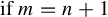 $\text {if } m=n+1$
.
$\text {if } m=n+1$
.
Lemma 3.10 immediately implies the following, somewhat stronger lemma.
Lemma 3.11. Let a
 $C^r$
map
$C^r$
map
 $f_0$
, where
$f_0$
, where
 $r=3,\ldots ,\infty ,\omega $
, have a bi-focus periodic orbit
$r=3,\ldots ,\infty ,\omega $
, have a bi-focus periodic orbit
 $L_{f_0}$
whose stable and unstable manifolds
$L_{f_0}$
whose stable and unstable manifolds
 $W^s(L_{f_0})$
and
$W^s(L_{f_0})$
and
 $W^u(L_{f_0})$
contain
$W^u(L_{f_0})$
contain
 $h=2l$
,
$h=2l$
,
 $l\in \mathbb N$
, orbits
$l\in \mathbb N$
, orbits
 $\Gamma ^1, \ldots \Gamma ^h$
of corank-2 homoclinic tangency satisfying conditions (C1) and (C2). Let these tangencies be of index
$\Gamma ^1, \ldots \Gamma ^h$
of corank-2 homoclinic tangency satisfying conditions (C1) and (C2). Let these tangencies be of index
 $(n,m)$
, where
$(n,m)$
, where
 $1\le n\le r-2$
and
$1\le n\le r-2$
and
 $0\le m\le n+1$
. Let the map
$0\le m\le n+1$
. Let the map
 $f_0$
be included in a finite-parameter
$f_0$
be included in a finite-parameter
 $C^r$
family of maps
$C^r$
family of maps
 $f_{\varepsilon }$
, which is proper for the global maps
$f_{\varepsilon }$
, which is proper for the global maps
 $T_{\Gamma ^1}, \ldots , T_{\Gamma ^h}$
. Then, there exists arbitrarily small
$T_{\Gamma ^1}, \ldots , T_{\Gamma ^h}$
. Then, there exists arbitrarily small
 $\varepsilon ^{*}$
such that
$\varepsilon ^{*}$
such that
 $W^s(L_{f_{\varepsilon ^{*}}})$
and
$W^s(L_{f_{\varepsilon ^{*}}})$
and
 $W^u(L_{f_{\varepsilon ^{*}}})$
contain
$W^u(L_{f_{\varepsilon ^{*}}})$
contain
 ${h}/{2}$
orbits of corank-2 homoclinic tangency of index not lower than
${h}/{2}$
orbits of corank-2 homoclinic tangency of index not lower than
 $(n,m+1)$
 $\text {if } 0\le m\le n$
, or
$\text {if } 0\le m\le n$
, or
 $(n+1,0)$
 $\text {if } m=n+1$
.
$\text {if } m=n+1$
.
For a proof, just notice that since the parametric family
 $f_{\varepsilon }$
is proper for the global maps
$f_{\varepsilon }$
is proper for the global maps
 $T_{\Gamma ^1}, \ldots , T_{\Gamma ^h}$
, one can perturb freely and independently any pair of global maps while keeping all other global maps (or, more precisely, the corresponding splitting coefficients) unperturbed.
$T_{\Gamma ^1}, \ldots , T_{\Gamma ^h}$
, one can perturb freely and independently any pair of global maps while keeping all other global maps (or, more precisely, the corresponding splitting coefficients) unperturbed.
Lemma 3.12. Let a
 $C^r$
map f, where
$C^r$
map f, where
 $r=2,\ldots ,\infty ,\omega $
, have a bi-focus periodic orbit
$r=2,\ldots ,\infty ,\omega $
, have a bi-focus periodic orbit
 $L_{f}$
whose stable and unstable manifolds
$L_{f}$
whose stable and unstable manifolds
 $W^s(L_{f})$
and
$W^s(L_{f})$
and
 $W^u(L_{f})$
contain
$W^u(L_{f})$
contain
 $h=2^{{(n-1)(n+4)}/{2}}$
orbits of corank-2 homoclinic tangency satisfying conditions (C1) and (C2). Let these tangencies be of index
$h=2^{{(n-1)(n+4)}/{2}}$
orbits of corank-2 homoclinic tangency satisfying conditions (C1) and (C2). Let these tangencies be of index
 $(1,0)$
, where
$(1,0)$
, where
 $1\le n\le r-1$
. Then, arbitrarily
$1\le n\le r-1$
. Then, arbitrarily
 $C^r$
-close to f, there exists a map g such that
$C^r$
-close to f, there exists a map g such that
 $W^s(L_g)$
and
$W^s(L_g)$
and
 $W^u(L_g)$
contain an orbit of corank-2 homoclinic tangency of index
$W^u(L_g)$
contain an orbit of corank-2 homoclinic tangency of index
 $(n,0)$
.
$(n,0)$
.
Proof. First, we note that each non-negative integer k can be uniquely represented as
 $$ \begin{align} \begin{aligned} &k=\frac{(j-1)(j+4)}{2}+i,\\ \end{aligned} \end{align} $$
where j and i are integers satisfying
 $j\ge 1$
and
$j\ge 1$
and
 $0\le i\le j+1$
.
$0\le i\le j+1$
.
Let
 $n=1$
. Then, the map f has one orbit of corank-2 homoclinic tangency of index
$n=1$
. Then, the map f has one orbit of corank-2 homoclinic tangency of index
 $(1,0)$
, so the lemma holds trivially. Assume that
$(1,0)$
, so the lemma holds trivially. Assume that
 $n>1$
. To construct a map g with the required properties, we specify an algorithm consisting of
$n>1$
. To construct a map g with the required properties, we specify an algorithm consisting of
 $l={(n-1)(n+4)}/{2}$
steps. At the kth step
$l={(n-1)(n+4)}/{2}$
steps. At the kth step
 $(1\le k\le l)$
, we add several
$(1\le k\le l)$
, we add several
 $C^{r}$
-small perturbations to construct a map
$C^{r}$
-small perturbations to construct a map
 $f_k$
with
$f_k$
with
 $h_k={h}/{2^k}$
orbits of corank-2 homoclinic tangency of index
$h_k={h}/{2^k}$
orbits of corank-2 homoclinic tangency of index
 $(j,i)$
, where the numbers
$(j,i)$
, where the numbers
 $i,j,k$
are related by equation (50). After performing this algorithm l times, we obtain a map
$i,j,k$
are related by equation (50). After performing this algorithm l times, we obtain a map
 $g\equiv f_{l}$
, which is
$g\equiv f_{l}$
, which is
 $C^r$
-close to the map f and which has
$C^r$
-close to the map f and which has
 $h_{l}=1$
orbit of corank-2 homoclinic tangency of index
$h_{l}=1$
orbit of corank-2 homoclinic tangency of index
 $(n,0)$
.
$(n,0)$
.
Further, we describe in detail the perturbations that we add at the step k, where
 ${1\le k\le l}$
. Let
${1\le k\le l}$
. Let
 $f_0=f$
and
$f_0=f$
and
 $h_0=h$
. Let
$h_0=h$
. Let
 $j,i$
be a pair of integers such that
$j,i$
be a pair of integers such that
 $i,j,k$
are related by equation (50). After the
$i,j,k$
are related by equation (50). After the
 $(k-1)$
th step, we have a map
$(k-1)$
th step, we have a map
 $f_{k-1}$
with
$f_{k-1}$
with
 $h_{k-1}={h}/{2^{k-1}}$
orbits
$h_{k-1}={h}/{2^{k-1}}$
orbits
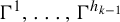 $\Gamma ^1,\ldots ,\Gamma ^{h_{k-1}}$
of corank-2 tangency of index
$\Gamma ^1,\ldots ,\Gamma ^{h_{k-1}}$
of corank-2 tangency of index
 $(j-1,j)$
if
$(j-1,j)$
if
 $i=0$
, and
$i=0$
, and
 $(j,i-1)$
if
$(j,i-1)$
if
 $1\le i\le j+1$
.
$1\le i\le j+1$
.
Step k. Applying Lemma 3.8, include the map
 $f_{k-1}$
in a finite-parameter
$f_{k-1}$
in a finite-parameter
 $C^r$
family of maps, which is proper for the global maps
$C^r$
family of maps, which is proper for the global maps
 $T_{\Gamma ^1},\ldots ,T_{\Gamma ^{h_{k-1}}}$
. By Lemma 3.11, in this family, we find a map
$T_{\Gamma ^1},\ldots ,T_{\Gamma ^{h_{k-1}}}$
. By Lemma 3.11, in this family, we find a map
 $\tilde f_{k}$
, which is
$\tilde f_{k}$
, which is
 $C^r$
-close to
$C^r$
-close to
 $f_{k-1}$
and has
$f_{k-1}$
and has
 $h_k={h}/{2^{k}}$
orbits
$h_k={h}/{2^{k}}$
orbits
 $\tilde \Gamma ^1,\ldots ,\tilde \Gamma ^{h_k}$
of corank-2 homoclinic tangency of index not lower than
$\tilde \Gamma ^1,\ldots ,\tilde \Gamma ^{h_k}$
of corank-2 homoclinic tangency of index not lower than
 $(j,0)$
if
$(j,0)$
if
 $i=0$
, or
$i=0$
, or
 $(j,i)$
if
$(j,i)$
if
 ${1\le i\le j+1}$
. Using Lemma 3.8, include the map
${1\le i\le j+1}$
. Using Lemma 3.8, include the map
 $\tilde f_k$
in a finite-parameter
$\tilde f_k$
in a finite-parameter
 $C^r$
family that perturbs the global maps
$C^r$
family that perturbs the global maps
 $T_{\tilde \Gamma ^1},\ldots ,T_{\tilde \Gamma ^{h_k}}$
freely and independently up to index
$T_{\tilde \Gamma ^1},\ldots ,T_{\tilde \Gamma ^{h_k}}$
freely and independently up to index
 $(j,i+1)$
if
$(j,i+1)$
if
 $0\le i\le j$
, or
$0\le i\le j$
, or
 $(j+1,0)$
if
$(j+1,0)$
if
 $i=j+1$
. Slightly changing parameters in this family, we can always make
$i=j+1$
. Slightly changing parameters in this family, we can always make
 ${\partial ^{j+1} (F_1,F_2)}/{\partial y^{j+1-i}_1 \partial y^{i}_2}\not =(0,0)$
at the point
${\partial ^{j+1} (F_1,F_2)}/{\partial y^{j+1-i}_1 \partial y^{i}_2}\not =(0,0)$
at the point
 $(y_1,y_2)=(y^-_1,y^-_2)$
, where
$(y_1,y_2)=(y^-_1,y^-_2)$
, where
 $0\le i\le j+1$
, for each of the orbits
$0\le i\le j+1$
, for each of the orbits
 $\tilde \Gamma ^1,\ldots ,\tilde \Gamma ^{h_k}$
(see Definition 3.5). As a result, we get the map
$\tilde \Gamma ^1,\ldots ,\tilde \Gamma ^{h_k}$
(see Definition 3.5). As a result, we get the map
 $f_k$
with
$f_k$
with
 $h_k$
orbits of corank-2 homoclinic tangency of index exactly
$h_k$
orbits of corank-2 homoclinic tangency of index exactly
 $(j,i)$
, where
$(j,i)$
, where
 $0\le i\le j+1$
.
$0\le i\le j+1$
.
It completes the proof of the lemma.
Proof of Theorem 1.2
Let f be a
 $C^r$
map
$C^r$
map
 $(r=2,\ldots ,\infty ,\omega )$
having a bi-focus periodic orbit
$(r=2,\ldots ,\infty ,\omega )$
having a bi-focus periodic orbit
 $L_f$
whose stable and unstable manifolds contain
$L_f$
whose stable and unstable manifolds contain
 $h=2^{{(n-1)(n+4)}/{2}}$
orbits of corank-2 homoclinic tangency. Making use of Lemma 3.8, we include the map f in a finite-parameter
$h=2^{{(n-1)(n+4)}/{2}}$
orbits of corank-2 homoclinic tangency. Making use of Lemma 3.8, we include the map f in a finite-parameter
 $C^r$
family, which perturbs the global maps corresponding to the given h orbits of corank-2 tangency freely and independently up to index
$C^r$
family, which perturbs the global maps corresponding to the given h orbits of corank-2 tangency freely and independently up to index
 $(1,1)$
. In this family,
$(1,1)$
. In this family,
 $C^r$
-close to f, we find a map
$C^r$
-close to f, we find a map
 $\tilde f$
with h orbits of corank-2 homoclinic tangency of index
$\tilde f$
with h orbits of corank-2 homoclinic tangency of index
 $(1,0)$
. Further, applying Lemma 3.12,
$(1,0)$
. Further, applying Lemma 3.12,
 $C^{r}$
-close to
$C^{r}$
-close to
 $\tilde f$
, we find a map g with an orbit of corank-2 homoclinic tangency of order n between the stable and unstable manifolds of
$\tilde f$
, we find a map g with an orbit of corank-2 homoclinic tangency of order n between the stable and unstable manifolds of
 $L_g$
.
$L_g$
.
4 Universal two-dimensional dynamics
Let f be a
 $C^r$
map
$C^r$
map
 $(r=2,\ldots ,\infty ,\omega )$
with a bi-focus periodic orbit
$(r=2,\ldots ,\infty ,\omega )$
with a bi-focus periodic orbit
 $L_f$
whose stable and unstable manifolds contain an orbit
$L_f$
whose stable and unstable manifolds contain an orbit
 $\Gamma $
of corank-2 homoclinic tangency. Let
$\Gamma $
of corank-2 homoclinic tangency. Let
 $O_f$
be a periodic point in the orbit
$O_f$
be a periodic point in the orbit
 $L_f$
, and let
$L_f$
, and let
 $\Pi ^{+}$
and
$\Pi ^{+}$
and
 $\Pi ^{-}$
be small neighbourhoods of the homoclinic points
$\Pi ^{-}$
be small neighbourhoods of the homoclinic points
 $M^+\in W^s_{\mathrm {loc}}(O_f)$
and
$M^+\in W^s_{\mathrm {loc}}(O_f)$
and
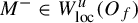 $M^-\in W^u_{\mathrm {loc}}(O_f)$
, respectively (see §3.2). By equation (19), the piece of
$M^-\in W^u_{\mathrm {loc}}(O_f)$
, respectively (see §3.2). By equation (19), the piece of
 $W^s_{\mathrm {loc}}(O_f)$
near
$W^s_{\mathrm {loc}}(O_f)$
near
 $M^+$
is the limit of the countable sequence of strips
$M^+$
is the limit of the countable sequence of strips
 $\sigma _k=\Pi ^+\cap T_0^{-k}\Pi ^-$
on which the first-return maps
$\sigma _k=\Pi ^+\cap T_0^{-k}\Pi ^-$
on which the first-return maps
 $T_k\equiv T_{\Gamma }\circ T_0^k$
are defined (see the discussion in [Reference Shilnikov, Shilnikov, Turaev and Chua44, §§3.8. and 3.9.]). The map
$T_k\equiv T_{\Gamma }\circ T_0^k$
are defined (see the discussion in [Reference Shilnikov, Shilnikov, Turaev and Chua44, §§3.8. and 3.9.]). The map
 $T_k$
takes the strip
$T_k$
takes the strip
 $\sigma _k\subset \Pi ^+$
back into
$\sigma _k\subset \Pi ^+$
back into
 $\Pi ^+$
. The same is true for all maps close to f.
$\Pi ^+$
. The same is true for all maps close to f.
To prove Theorem 1.7, we need explicit formulae for the first-return maps
 $T_{k}$
near corank-2 homoclinic tangencies of high orders. They are given by the following lemma.
$T_{k}$
near corank-2 homoclinic tangencies of high orders. They are given by the following lemma.
Lemma 4.1. Let a
 $C^r$
map
$C^r$
map
 $f_0$
, where
$f_0$
, where
 $r=2,\ldots ,\infty ,\omega $
, have a bi-focus periodic orbit
$r=2,\ldots ,\infty ,\omega $
, have a bi-focus periodic orbit
 $L_{f_0}$
whose stable and unstable manifolds contain an orbit
$L_{f_0}$
whose stable and unstable manifolds contain an orbit
 $\Gamma $
of corank-2 homoclinic tangency satisfying conditions (C1) and (C2). Let this tangency be of order n, where
$\Gamma $
of corank-2 homoclinic tangency satisfying conditions (C1) and (C2). Let this tangency be of order n, where
 $1\le n\le r-1$
. Let
$1\le n\le r-1$
. Let
 $f_0$
be included in a finite-parameter
$f_0$
be included in a finite-parameter
 $C^r$
family of maps
$C^r$
family of maps
 $f_{\varepsilon }$
, which perturbs the global map
$f_{\varepsilon }$
, which perturbs the global map
 $T_{\Gamma }$
freely up to order n. Then, for all sufficiently large
$T_{\Gamma }$
freely up to order n. Then, for all sufficiently large
 $k\in \mathbb N$
and all sufficiently small
$k\in \mathbb N$
and all sufficiently small
 $\varepsilon $
, there exist a
$\varepsilon $
, there exist a
 $C^{r}$
-smooth coordinate transformation on
$C^{r}$
-smooth coordinate transformation on
 $\sigma _{k}$
:
$\sigma _{k}$
:
 $(x,y,u,v)\rightarrow (X,Y,U,V)$
and a
$(x,y,u,v)\rightarrow (X,Y,U,V)$
and a
 $C^{r-n}$
-smooth transformation of the parameters
$C^{r-n}$
-smooth transformation of the parameters
 $\varepsilon \rightarrow M$
, which bring the first-return map
$\varepsilon \rightarrow M$
, which bring the first-return map
 $T_{k}$
to the form
$T_{k}$
to the form
 $$ \begin{align} \begin{aligned} \overline Y_1&=\sum\limits_{j=0}^n\sum\limits_{i=0}^{j} M_{1,j,i} Y_1^{j-i} Y_2^{i}+o(1)_{k\rightarrow+\infty},\\[4pt] \overline Y_2&=\sum\limits_{j=0}^n\sum\limits_{i=0}^{j} M_{2,j,i} Y_1^{j-i} Y_2^{i}+o(1)_{k\rightarrow+\infty},\\[4pt] (\overline X_1,\overline X_2,\overline U,V)&=o(1)_{k\rightarrow+\infty}. \\ \end{aligned} \end{align} $$
The range of values of the new variables
 $(X,Y,U,V)$
and parameters M covers a centred-at-zero ball whose radius tends to infinity as k increases. The
$(X,Y,U,V)$
and parameters M covers a centred-at-zero ball whose radius tends to infinity as k increases. The
 $o(1)$
-terms tend to zero uniformly on any compact, along with the derivatives with respect to
$o(1)$
-terms tend to zero uniformly on any compact, along with the derivatives with respect to
 $(X,Y,U,V)$
up to the order r and with respect to M up to the order
$(X,Y,U,V)$
up to the order r and with respect to M up to the order
 $r-n$
.
$r-n$
.
Proof. The family of maps
 $f_{\varepsilon }$
perturbs the global map
$f_{\varepsilon }$
perturbs the global map
 $T_{\Gamma }$
freely up to order n; therefore, using the condition (26), we can choose the splitting coefficients as the new independent parameters, that is,
$T_{\Gamma }$
freely up to order n; therefore, using the condition (26), we can choose the splitting coefficients as the new independent parameters, that is,
 $\varepsilon =\overline \mu _{n,0}$
. Combining formulae for the maps
$\varepsilon =\overline \mu _{n,0}$
. Combining formulae for the maps
 $T_0^k$
and
$T_0^k$
and
 $T_{\Gamma }$
, we get the following formula for the first-return map
$T_{\Gamma }$
, we get the following formula for the first-return map
 $T_{k}:(x_0,y_k,u_0,v_k)\mapsto (\overline x_0,\overline y_k,\overline u_0,\overline v_k)$
for all sufficiently large k and all small
$T_{k}:(x_0,y_k,u_0,v_k)\mapsto (\overline x_0,\overline y_k,\overline u_0,\overline v_k)$
for all sufficiently large k and all small
 $\varepsilon $
:
$\varepsilon $
:
 $$ \begin{align} &\overline x_{01}-x_1^+=b_{11} (y_{k1}-y_1^-)+b_{12} (y_{k2}-y_2^-)+O((y_k-y^-)^2)+O(\hat\gamma^{-k}),\nonumber\\[4pt] &\overline x_{02}-x_2^+=b_{21} (y_{k1}-y_1^-)+b_{22}(y_{k2}-y_2^-)+O((y_k-y^-)^2)+O(\hat\gamma^{-k}),\nonumber\\[4pt] &\gamma^{-k}\cdot(\overline y_{k1}\cos(k\psi)+\overline y_{k2}\sin(k\psi))=\sum\limits_{j=0}^n\sum\limits_{i=0}^{j} \mu_{1,j,i} (y_{k1}-y_1^-)^{j-i} (y_{k2}-y_2^-)^{i}\nonumber\\[4pt]&\qquad\qquad\qquad\qquad\qquad\qquad\qquad\quad+O(\|y_k-y^-\|^{n+1})+O(\hat\gamma^{-k}),\nonumber\\&\gamma^{-k}\cdot(-\overline y_{k1}\sin(k\psi)+\overline y_{k2}\cos(k\psi))=\sum\limits_{j=0}^n\sum\limits_{i=0}^{j} \mu_{2,j,i} (y_{k1}-y_1^-)^{j-i} (y_{k2}-y_2^-)^{i}\nonumber\\&\qquad\qquad\qquad\qquad\qquad\qquad\qquad\qquad+O(\|y_k-y^-\|^{n+1})+O(\hat\gamma^{-k}),\nonumber\\ &\overline u_0-u^+= b_{51}(y_{k1}-y_1^-)+b_{52}(y_{k2}-y_2^-)+O((y_k-y^-)^2)+O(\hat\gamma^{-k}),\nonumber\\ &v_k-v^-= b_{61}(y_{k1}-y_1^-)+b_{62}(y_{k2}-y_2^-)+O((y_k-y^-)^2)+O(\hat\gamma^{-k}).\nonumber\\ \end{align} $$
Making the change of the variables:
 $$ \begin{align*} \begin{aligned} &X=x_0-x^+, Y=y_k-y^-, U=u_0-u^+, V= v_k-v^-,\\ \end{aligned} \end{align*} $$
we rewrite the system in equation (52) as
 $$ \begin{align} \begin{aligned} \gamma^{-k}\cdot(\overline Y_1\cos(k\psi)+\overline Y_2\sin(k\psi))&=\sum\limits_{j=0}^n\sum\limits_{i=0}^{j} \hat{\mu}_{1,j,i} Y_1^{j-i} Y_2^{i}+\vartheta_1(X,Y,U,V,\overline X,\overline Y,\overline U,\overline V),\\ \gamma^{-k}\cdot(-\overline Y_1\sin(k\psi)+\overline Y_2\cos(k\psi))&=\sum\limits_{j=0}^n\sum\limits_{i=0}^{j} \hat{\mu}_{2,j,i} Y_1^{j-i} Y_2^{i}+\vartheta_2(X,Y,U,V,\overline X,\overline Y,\overline U,\overline V),\\ (\overline X_1,\overline X_2,\overline U,V)&=\vartheta_3(X,Y,U,V,\overline X,\overline Y,\overline U,\overline V), \end{aligned} \end{align} $$
where
 $$ \begin{align*} \begin{aligned} \hat \mu_{1,0,0}&=\mu_{1,0,0}-\gamma^{-k}(y_1^-\cos(k\psi)+y_2^-\sin(k\psi))+O(\hat\gamma^{-k}), \quad \hat{\mu}_{1,j,i}=\mu_{1,j,i}+O(\hat\gamma^{-k}),\\ \hat \mu_{2,0,0}&=\mu_{2,0,0}-\gamma^{-k}(-y_1^-\sin(k\psi)+y_2^-\cos(k\psi))+O(\hat\gamma^{-k}), \quad \hat{\mu}_{2,j,i}=\mu_{2,j,i}+O(\hat\gamma^{-k}),\\ \end{aligned} \end{align*} $$
and where the functions
 $\vartheta $
satisfy the estimates
$\vartheta $
satisfy the estimates
 $$ \begin{align*} \begin{aligned} &\vartheta_{1,2}=O(\|Y\|^{n+1})+O(\hat\gamma^{-k}) \quad \text{and} \quad \vartheta_3=O(\|Y\|)+O(\hat\gamma^{-k}).\\ \end{aligned} \end{align*} $$
Expressing
 $\overline Y_1$
,
$\overline Y_1$
,
 $\overline Y_2$
in the first and the second equations in equation (53), and applying the implicit function theorem, we recast the system in equation (53) as
$\overline Y_2$
in the first and the second equations in equation (53), and applying the implicit function theorem, we recast the system in equation (53) as
 $$ \begin{align} \begin{aligned} \gamma^{-k}\cdot\overline Y_1&=\sum\limits_{j=0}^n\sum\limits_{i=0}^{j} \tilde{\mu}_{1,j,i} Y_1^{j-i} Y_2^{i}+\tilde\vartheta_1(X,Y,U,\overline V),\\ \gamma^{-k}\cdot\overline Y_2&=\sum\limits_{j=0}^n\sum\limits_{i=0}^{j} \tilde{\mu}_{2,j,i} Y_1^{j-i} Y_2^{i}+\tilde\vartheta_2(X,Y,U,\overline V),\\ (\overline X_1,\overline X_2,\overline U,V)&=\tilde\vartheta_3(X,Y,U,\overline V),\\ \end{aligned} \end{align} $$
where
 $$ \begin{align*} \begin{aligned} \tilde \mu_{1,j,i}&=\hat{\mu}_{1,j,i}\cos(k\psi)-\hat{\mu}_{2,j,i}\sin(k\psi)+O(\hat\gamma^{-k}),\\ \tilde \mu_{2,j,i}&=\hat{\mu}_{1,j,i}\sin(k\psi)+\hat{\mu}_{2,j,i}\cos(k\psi)+O(\hat\gamma^{-k}),\\ \end{aligned} \end{align*} $$
and the functions
 $\tilde \vartheta $
satisfy
$\tilde \vartheta $
satisfy
 $$ \begin{align*} \begin{aligned} &\tilde \vartheta_{1,2}=O(\|Y\|^{n+1})+O(\hat\gamma^{-k}) \quad \text{and} \quad \tilde \vartheta_3=O(\|Y\|)+O(\gamma^k\hat\gamma^{-k}).\\ \end{aligned} \end{align*} $$
Further, let us nullify the constant terms in
 $\tilde \vartheta _3$
(by shifting the origin), and rescale the coordinates and the parameters as
$\tilde \vartheta _3$
(by shifting the origin), and rescale the coordinates and the parameters as
 $$ \begin{align*}&(Y_1,Y_2)=\gamma^{-{2k}/{n}}\cdot(Y^{\mathrm{new}}_1,Y^{\mathrm{new}}_2), (X_1,X_2,U,V)=\frac{\gamma^{-{2k}/{n}}}{\delta_k}\cdot(X^{\mathrm{new}}_1,X^{\mathrm{new}}_2,U^{\mathrm{new}},V^{\mathrm{new}}),\end{align*} $$
 $$ \begin{align*}& (\tilde{\mu}_{1,j,i},\tilde{\mu}_{2,j,i})=\gamma^{-k(1-{2(j-1)}/{n})}\cdot(M_{1,j,i},M_{2,j,i}),\end{align*} $$
where
 $\delta _{k}$
tends sufficiently slowly to zero as
$\delta _{k}$
tends sufficiently slowly to zero as
 $k\rightarrow +\infty $
. After it, the system in equation (54) is reduced to the desired form in equation (51).
$k\rightarrow +\infty $
. After it, the system in equation (54) is reduced to the desired form in equation (51).
Proof of Theorem 1.7
Let us fix
 $k\in \mathbb N$
,
$k\in \mathbb N$
,
 $k\ge 4$
, and let
$k\ge 4$
, and let
 $U^k$
be a unit ball in
$U^k$
be a unit ball in
 $\mathbb R^k$
. Let us fix
$\mathbb R^k$
. Let us fix
 $r=2,\ldots ,\infty ,\omega $
. Let us take any
$r=2,\ldots ,\infty ,\omega $
. Let us take any
 $\delta>0$
and any
$\delta>0$
and any
 $C^r$
map
$C^r$
map
 $\zeta :U^k\rightarrow \mathbb R^k$
of the form
$\zeta :U^k\rightarrow \mathbb R^k$
of the form
 $$ \begin{align} \begin{aligned} (\overline X_1,\ldots,\overline X_{k-2})&= 0, \\ (\overline X_{k-1},\overline X_k)&= \Phi (X_{k-1},X_k),\\ \end{aligned} \end{align} $$
where
 $\Phi : U^2\rightarrow \mathbb R^2$
is an arbitrary
$\Phi : U^2\rightarrow \mathbb R^2$
is an arbitrary
 $C^r$
map. Let
$C^r$
map. Let
 $\mathcal H(\zeta ,\delta )$
be the set of all k-dimensional
$\mathcal H(\zeta ,\delta )$
be the set of all k-dimensional
 $C^r$
maps such that for each map from
$C^r$
maps such that for each map from
 $\mathcal H(\zeta ,\delta )$
, there exists its renormalized iteration that is at distance smaller than
$\mathcal H(\zeta ,\delta )$
, there exists its renormalized iteration that is at distance smaller than
 $\delta $
from
$\delta $
from
 $\zeta $
(in the
$\zeta $
(in the
 $C^r$
topology). By definition, the set
$C^r$
topology). By definition, the set
 $\mathcal H(\zeta ,\delta )$
is open. Let us prove that this set is dense in the
$\mathcal H(\zeta ,\delta )$
is open. Let us prove that this set is dense in the
 $ABR^{*}$
-domain.
$ABR^{*}$
-domain.
Let f be any map belonging to the
 $ABR^{*}$
-domain. By Theorem 1.4, arbitrarily
$ABR^{*}$
-domain. By Theorem 1.4, arbitrarily
 $C^r$
-close to f, there exists a real-analytic map g that has infinitely many orbits of corank-2 tangency of every order. Let
$C^r$
-close to f, there exists a real-analytic map g that has infinitely many orbits of corank-2 tangency of every order. Let
 $\Gamma $
be one of these orbits and let the tangency be of order n, where n is sufficiently large. Using Lemma 3.8, include the map g in a finite-parameter analytic family
$\Gamma $
be one of these orbits and let the tangency be of order n, where n is sufficiently large. Using Lemma 3.8, include the map g in a finite-parameter analytic family
 $g_{\varepsilon }$
 $(g_0=g)$
, which perturbs the global map
$(g_0=g)$
, which perturbs the global map
 $T_{\Gamma }$
freely up to order n. Then, according to Lemma 4.1, for all small
$T_{\Gamma }$
freely up to order n. Then, according to Lemma 4.1, for all small
 $\varepsilon $
, the corresponding first-return map in some coordinates (after rescaling) is arbitrarily close to
$\varepsilon $
, the corresponding first-return map in some coordinates (after rescaling) is arbitrarily close to
 $$ \begin{align*} \begin{aligned} &\overline Y_1=\sum\limits_{j=0}^n\sum\limits_{i=0}^{j} M_{1,j,i} Y_1^{j-i} Y_2^{i}, \overline Y_2=\sum\limits_{j=0}^n\sum\limits_{i=0}^{j} M_{2,j,i} Y_1^{j-i} Y_2^{i}, (\overline X_1,\overline X_2,\overline U,V)=0. \\ \end{aligned} \end{align*} $$
Changing the rescaled parameters
 $M_{1,j,i}$
and
$M_{1,j,i}$
and
 $M_{2,j,i}$
, considering that n can be arbitrarily large and applying the Stone–Weierstrass theorem (if
$M_{2,j,i}$
, considering that n can be arbitrarily large and applying the Stone–Weierstrass theorem (if
 $r=2,\ldots ,\infty $
) or the Oka–Weil theorem (if
$r=2,\ldots ,\infty $
) or the Oka–Weil theorem (if
 $r=\omega $
), we obtain that arbitrarily
$r=\omega $
), we obtain that arbitrarily
 $C^r$
-close to f, there exists a map such that its certain renormalized iteration approximates the map
$C^r$
-close to f, there exists a map such that its certain renormalized iteration approximates the map
 $\zeta $
with arbitrarily good accuracy. Thus, the set
$\zeta $
with arbitrarily good accuracy. Thus, the set
 $\mathcal H(\zeta ,\delta )$
is dense in the
$\mathcal H(\zeta ,\delta )$
is dense in the
 $ABR^{*}$
-domain.
$ABR^{*}$
-domain.
Let us take a sequence of maps
 $(\zeta _i)_{i\in \mathbb N}$
such that it is dense in the space of
$(\zeta _i)_{i\in \mathbb N}$
such that it is dense in the space of
 $C^r$
maps of the form in equation (55) and converging to zero sequence
$C^r$
maps of the form in equation (55) and converging to zero sequence
 $(\delta _j)_{j\in \mathbb N}$
, where
$(\delta _j)_{j\in \mathbb N}$
, where
 $\delta _j$
is a positive real number. Then, the intersection
$\delta _j$
is a positive real number. Then, the intersection
 $\bigcap \nolimits _{i,j}\mathcal H(\zeta _i,\delta _j)$
is a residual set in the
$\bigcap \nolimits _{i,j}\mathcal H(\zeta _i,\delta _j)$
is a residual set in the
 $ABR^{*}$
-domain and consists of maps having
$ABR^{*}$
-domain and consists of maps having
 $C^r$
-universal two-dimensional dynamics. This completes the proof of the theorem.
$C^r$
-universal two-dimensional dynamics. This completes the proof of the theorem.
Acknowledgments
I am grateful to my scientific adviser Dmitry Turaev for setting the problem, his valuable comments and constant support. I would like to thank the referee for illuminating questions and remarks that significantly improved this article. Also, I would like to thank M. Asaoka, P. Berger, S.V. Gonchenko, N. Gourmelon, V.P.H. Goverse, M. Helfter, A. Khodaeian Karim, J.S.W. Lamb, D. Li and S. van Strien for useful discussions. The research was supported by the EPSRC Centre for Doctoral Training in Mathematics of Random Systems: Analysis, Modelling and Simulation (EP/S023925/1), RSF grant (project 22-11-00027) and Leverhulme Trust grant RPG-2021-072.
A Appendix. Corank-c homoclinic tangency is a bifurcation of codimension
$c^2$

In this section, we explain why the corank-c homoclinic tangency is a bifurcation of codimension
 $c^2$
. We recall that the codimension of a bifurcation happening in a generic parametric family is the difference between the dimension of the parameter space and the dimension of the corresponding bifurcation boundary (cf. [Reference Arnold, Afraimovich, Ilyashenko and Shilnikov2, Reference Kuznetsov31]).
$c^2$
. We recall that the codimension of a bifurcation happening in a generic parametric family is the difference between the dimension of the parameter space and the dimension of the corresponding bifurcation boundary (cf. [Reference Arnold, Afraimovich, Ilyashenko and Shilnikov2, Reference Kuznetsov31]).
Let
 $\mathcal M^k$
be a smooth or analytic k-dimensional manifold and let
$\mathcal M^k$
be a smooth or analytic k-dimensional manifold and let
 $\mathcal D^l$
be an l-dimensional ball. Let
$\mathcal D^l$
be an l-dimensional ball. Let
 $\mathcal P_{l,r}$
be the space of all l-parameter
$\mathcal P_{l,r}$
be the space of all l-parameter
 $C^r$
families
$C^r$
families
 $(l\in \mathbb N, r=2,\ldots ,\infty ,\omega )$
of diffeomorphisms of the manifold
$(l\in \mathbb N, r=2,\ldots ,\infty ,\omega )$
of diffeomorphisms of the manifold
 $\mathcal M^k$
. Let
$\mathcal M^k$
. Let
 $\varepsilon $
be a vector of parameters that is defined on the ball
$\varepsilon $
be a vector of parameters that is defined on the ball
 $\mathcal D^l$
. Any family of maps
$\mathcal D^l$
. Any family of maps
 $f_{\varepsilon }\in \mathcal P_{l,r}$
can be considered as a map
$f_{\varepsilon }\in \mathcal P_{l,r}$
can be considered as a map
 $\mathcal M^k\times \mathcal D^l\to \mathcal M^k\times \mathcal D^l$
, which acts as
$\mathcal M^k\times \mathcal D^l\to \mathcal M^k\times \mathcal D^l$
, which acts as
 $(x,\varepsilon )\mapsto (f(x,\varepsilon ),\varepsilon )$
with a
$(x,\varepsilon )\mapsto (f(x,\varepsilon ),\varepsilon )$
with a
 $C^r$
map
$C^r$
map
 $f:$
$f:$
 $\mathcal M^k\times \mathcal D^l\to \mathcal M^k$
(see §1.2). Therefore, we can introduce the
$\mathcal M^k\times \mathcal D^l\to \mathcal M^k$
(see §1.2). Therefore, we can introduce the
 $C^r$
topology on the space of such maps.
$C^r$
topology on the space of such maps.
Let
 $f_{\varepsilon }$
be a
$f_{\varepsilon }$
be a
 $C^r$
family of maps such that
$C^r$
family of maps such that
 $f_0$
has a hyperbolic saddle periodic orbit
$f_0$
has a hyperbolic saddle periodic orbit
 $L_{f_0}$
. Let the stable and unstable manifolds
$L_{f_0}$
. Let the stable and unstable manifolds
 $W^s(L_{f_0})$
and
$W^s(L_{f_0})$
and
 $W^u(L_{f_0})$
contain an orbit
$W^u(L_{f_0})$
contain an orbit
 $\Gamma $
of corank-c homoclinic tangency. Our goal is to show that for a generic family of maps
$\Gamma $
of corank-c homoclinic tangency. Our goal is to show that for a generic family of maps
 $f_{\varepsilon }$
with the properties above, we obtain the following.
$f_{\varepsilon }$
with the properties above, we obtain the following.
-
(1) If
$l\ge c^2$
, then there exists a
$C^{r-1}$
-smooth
$(l-c^2)$
-dimensional embedded disk
${\mathcal S\subset \mathcal D^l}$
such that:-
(I) for each
$\varepsilon ^{*}\in \mathcal S$
, the manifolds
$W^s(L_{f_{\varepsilon ^{*}}})$
and
$W^u(L_{f_{\varepsilon ^{*}}})$
contain an orbit of corank-c tangency that is a continuation of the orbit
$\Gamma $
; -
(II)
$\mathcal S$
passes through
$\varepsilon =0$
.
-
-
(2) If
$l< c^2$
, then arbitrarily
$C^r$
-close to
$f_{\varepsilon }$
, there exists a
$C^r$
family of maps
$h_{\varepsilon }$
such that for all small
$\varepsilon $
, the manifolds
$W^s(L_{h_{\varepsilon }})$
and
$W^u(L_{h_{\varepsilon }})$
do not contain an orbit of corank-c tangency that is a continuation of the orbit
$\Gamma $
.


Let
 $k_s$
be the dimension of the manifold
$k_s$
be the dimension of the manifold
 $W^s(L_{f_{\varepsilon }})$
and
$W^s(L_{f_{\varepsilon }})$
and
 $k_u$
be the dimension of the manifold
$k_u$
be the dimension of the manifold
 $W^u(L_{f_{\varepsilon }})$
. Fix a point
$W^u(L_{f_{\varepsilon }})$
. Fix a point
 $M\in \Gamma $
. As in §2.1, near this point, we introduce the coordinates
$M\in \Gamma $
. As in §2.1, near this point, we introduce the coordinates
 $(z\in \mathbb R^c,\hat z\in \mathbb R^{k_s-c},w\in \mathbb R^c,\hat w\in \mathbb R^{k_u-c})$
such that
$(z\in \mathbb R^c,\hat z\in \mathbb R^{k_s-c},w\in \mathbb R^c,\hat w\in \mathbb R^{k_u-c})$
such that
 $W^s(L_{f_{\varepsilon }})$
and
$W^s(L_{f_{\varepsilon }})$
and
 $W^u(L_{f_{\varepsilon }})$
for all small
$W^u(L_{f_{\varepsilon }})$
for all small
 $\varepsilon $
take the form
$\varepsilon $
take the form
 $$ \begin{align*} \begin{aligned} W^s(L_{f_{\varepsilon}})&=\{(w,\hat w)=(0,0)\},\\ W^u(L_{f_{\varepsilon}})&=\{w=g_{1,\varepsilon}(z,\hat w), \hat z=g_{2,\varepsilon}(z,\hat w)\}, \end{aligned} \end{align*} $$
where the functions
 $g_{1,\varepsilon }, g_{2,\varepsilon }$
are of class
$g_{1,\varepsilon }, g_{2,\varepsilon }$
are of class
 $C^r$
with respect to the coordinates and parameters. Similarly to the corank-2 case, we introduce the splitting function
$C^r$
with respect to the coordinates and parameters. Similarly to the corank-2 case, we introduce the splitting function
 $$ \begin{align*} \begin{aligned} &G_{\varepsilon}(z)=g_{1,\varepsilon}(z,0). \end{aligned} \end{align*} $$
The manifolds
 $W^s(L_{f_{\varepsilon }})$
and
$W^s(L_{f_{\varepsilon }})$
and
 $W^u(L_{f_{\varepsilon }})$
have a corank-c tangency at the point M at
$W^u(L_{f_{\varepsilon }})$
have a corank-c tangency at the point M at
 $\varepsilon =0$
, so
$\varepsilon =0$
, so
 $$ \begin{align*} \begin{aligned} &G_0(0)=0 \quad \text{and} \quad \frac{\partial G_0}{\partial z}\bigg|_{z=0}=0. \end{aligned} \end{align*} $$
For small
 $\varepsilon $
, the function
$\varepsilon $
, the function
 $G_{\varepsilon }$
can be written as
$G_{\varepsilon }$
can be written as
 $$ \begin{align*} \begin{aligned} &G_{\varepsilon}(z)=\eta_0+\eta_1 \cdot z+\begin{pmatrix} z^T \cdot Q_1\cdot z \\ \vdots \\ z^T\cdot Q_c\cdot z \end{pmatrix}+o(z^{2}), \end{aligned} \end{align*} $$
where
 $$ \begin{align*} \begin{aligned} &\eta_0=\begin{pmatrix} \eta_{1,0,1}\\ \vdots \\ \eta_{c,0,1} \end{pmatrix}_{c\times 1} \quad \text{and} \quad \eta_1=\begin{pmatrix} \eta_{1,1,1} & \cdots& \eta_{1,1,c}\\ \vdots & \ddots & \vdots\\ \eta_{c,1,1} & \cdots& \eta_{c,1,c} \end{pmatrix}_{c\times c} \end{aligned} \end{align*} $$
are smooth functions of
 $\varepsilon $
vanishing at
$\varepsilon $
vanishing at
 $\varepsilon =0$
;
$\varepsilon =0$
;
 $Q_1,\ldots ,Q_c$
are symmetric
$Q_1,\ldots ,Q_c$
are symmetric
 $c\times c$
matrices depending continuously on
$c\times c$
matrices depending continuously on
 $\varepsilon $
. Let us require the following genericity condition.
$\varepsilon $
. Let us require the following genericity condition.
Condition A.1. The quadratic form
 $Q_1$
is non-degenerate.
$Q_1$
is non-degenerate.
We note that the Condition A.1 is not optimal, but is sufficient for our purpose.
The map
 $f_{\varepsilon }$
has a tangency (which is a continuation of
$f_{\varepsilon }$
has a tangency (which is a continuation of
 $\Gamma $
) at the point
$\Gamma $
) at the point
 $z=z^{*}$
if and only if after the shift of the origin of z-coordinate to this point, the corresponding values of
$z=z^{*}$
if and only if after the shift of the origin of z-coordinate to this point, the corresponding values of
 $\eta _0$
and
$\eta _0$
and
 $\eta _1$
, which we denote by
$\eta _1$
, which we denote by
 $\eta ^{*}_0$
and
$\eta ^{*}_0$
and
 $\eta ^{*}_1$
, get nullified. In particular, the first row of the matrix
$\eta ^{*}_1$
, get nullified. In particular, the first row of the matrix
 $\eta ^{*}_1$
becomes zero. Note that this row is given by
$\eta ^{*}_1$
becomes zero. Note that this row is given by
 $\eta ^{*}_{1,1}=\eta _{1,1}+2\cdot Q_1\cdot z^{*}+o(z^{*})$
. Since
$\eta ^{*}_{1,1}=\eta _{1,1}+2\cdot Q_1\cdot z^{*}+o(z^{*})$
. Since
 $\det Q_1\not =0$
, the value of the candidate for the tangency point
$\det Q_1\not =0$
, the value of the candidate for the tangency point
 $z=z^{*}$
is defined uniquely for all small
$z=z^{*}$
is defined uniquely for all small
 $\varepsilon $
.
$\varepsilon $
.
From now on, we assume that the coordinate system is chosen such that the point
 $z=z^{*}$
is at the origin. Hence, the splitting function
$z=z^{*}$
is at the origin. Hence, the splitting function
 $G_{\varepsilon }$
takes the form
$G_{\varepsilon }$
takes the form
 $$ \begin{align*} \begin{aligned} &G_{\varepsilon}(z)=\eta^{*}_0+\eta^{*}_1 \cdot z+\begin{pmatrix} z^T \cdot Q_1\cdot z \\ \vdots \\ z^T\cdot Q_c\cdot z \end{pmatrix}+o(z^{2}), \end{aligned} \end{align*} $$
where
 $$ \begin{align*} \begin{aligned} &\eta^{*}_0=\begin{pmatrix} \eta^{*}_{1,0,1}\\ \vdots \\ \eta^{*}_{c,0,1} \end{pmatrix}_{c\times 1} \quad \text{and} \quad \eta^{*}_1=\begin{pmatrix} 0 & \cdots& 0\\ \eta^{*}_{2,1,1} & \cdots& \eta^{*}_{2,1,c}\\ \vdots & \ddots & \vdots\\ \eta^{*}_{c,1,1} & \cdots& \eta^{*}_{c,1,c} \end{pmatrix}_{c\times c}. \end{aligned} \end{align*} $$
Let
 $\overline \eta \in \mathbb R^{c^2}$
be a vector that consists of all the coefficients of the matrix
$\overline \eta \in \mathbb R^{c^2}$
be a vector that consists of all the coefficients of the matrix
 $\eta ^{*}_0$
, and all the coefficients of the matrix
$\eta ^{*}_0$
, and all the coefficients of the matrix
 $\eta ^{*}_1$
except the zero first row. By the construction, the map
$\eta ^{*}_1$
except the zero first row. By the construction, the map
 $f_{\varepsilon }$
has a corank-c homoclinic tangency, which is a continuation of
$f_{\varepsilon }$
has a corank-c homoclinic tangency, which is a continuation of
 $\Gamma $
if and only if
$\Gamma $
if and only if
 $$ \begin{align} \begin{aligned} &\overline\eta=0. \end{aligned} \end{align} $$
Define a
 $c^2\times l$
matrix
$c^2\times l$
matrix
 $B={\partial \overline \eta }/{\partial \varepsilon } |_{\varepsilon =0}$
. The second genericity condition is as follows.
$B={\partial \overline \eta }/{\partial \varepsilon } |_{\varepsilon =0}$
. The second genericity condition is as follows.
Condition A.2. The matrix B has full rank.
Proof of item (1). Let
 $l\ge c^2$
. Condition A.2 means that the matrix B has a non-zero minor determinant of order
$l\ge c^2$
. Condition A.2 means that the matrix B has a non-zero minor determinant of order
 $c^2$
. By renumbering the parameters, we get
$c^2$
. By renumbering the parameters, we get
 $$ \begin{align*} \begin{aligned} &\det\frac{\partial\overline\eta}{\partial\varepsilon_1}\bigg|_{\varepsilon=0}\not=0, \end{aligned} \end{align*} $$
where
 $\varepsilon =(\varepsilon _1,\varepsilon _2)$
with
$\varepsilon =(\varepsilon _1,\varepsilon _2)$
with
 $\varepsilon _1\in \mathbb R^{c^2}$
and
$\varepsilon _1\in \mathbb R^{c^2}$
and
 $\varepsilon _2\in \mathbb R^{l-c^2}$
. Applying the implicit function theorem, we obtain that the solution to equation (A.1) is given by
$\varepsilon _2\in \mathbb R^{l-c^2}$
. Applying the implicit function theorem, we obtain that the solution to equation (A.1) is given by
 $$ \begin{align*} \begin{aligned} &\varepsilon_1=\mathcal H(\varepsilon_2), \end{aligned} \end{align*} $$
where
 $\mathcal H$
is a
$\mathcal H$
is a
 $C^{r-1}$
function such that
$C^{r-1}$
function such that
 $\mathcal H(0)=0$
. Clearly, this defines the disk
$\mathcal H(0)=0$
. Clearly, this defines the disk
 $\mathcal S$
satisfying the required properties (I) and (II).
$\mathcal S$
satisfying the required properties (I) and (II).
Proof of item (2). Let
 $l< c^2$
. The Condition A.2 means that the matrix B has non-zero minor determinant of order l. By renumbering the coefficients in the matrix
$l< c^2$
. The Condition A.2 means that the matrix B has non-zero minor determinant of order l. By renumbering the coefficients in the matrix
 $\overline \eta $
, we get
$\overline \eta $
, we get
 $$ \begin{align*} \begin{aligned} &\det\frac{\partial\overline\eta_1}{\partial\varepsilon}\bigg|_{\varepsilon=0}\not=0, \end{aligned} \end{align*} $$
where
 $\overline \eta =(\overline \eta ^1,\overline \eta ^2)$
with
$\overline \eta =(\overline \eta ^1,\overline \eta ^2)$
with
 $\overline \eta ^1\in \mathbb R^l$
and
$\overline \eta ^1\in \mathbb R^l$
and
 $\overline \eta ^2\in \mathbb R^{c^2-l}$
. By the implicit function theorem,
$\overline \eta ^2\in \mathbb R^{c^2-l}$
. By the implicit function theorem,
 ${\overline \eta _1=0}$
if and only if
${\overline \eta _1=0}$
if and only if
 $\varepsilon =0$
. So, perturbing the family
$\varepsilon =0$
. So, perturbing the family
 $f_{\varepsilon }$
in such a way that
$f_{\varepsilon }$
in such a way that
 $\overline \eta _2(\varepsilon =0)\not =0$
, we get that equation (A.1) has no solution for all small
$\overline \eta _2(\varepsilon =0)\not =0$
, we get that equation (A.1) has no solution for all small
 $\varepsilon $
.
$\varepsilon $
.


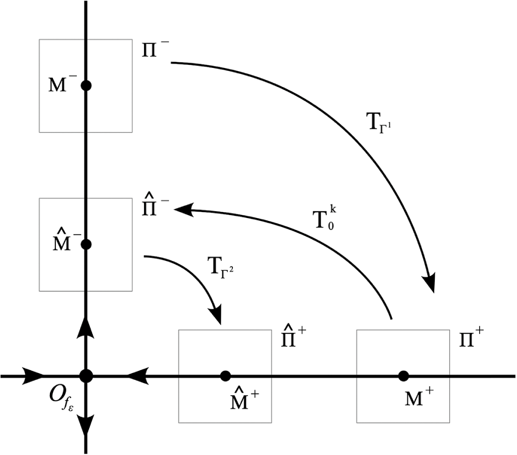


 Open access