





1 Introduction
In this paper, we investigate a one-dimensional discrete Schrödinger operator with dynamically defined potentials. Consider a measurable dynamical system
$(\Omega , T, \mu )$
 with an invertible map
$T:\Omega \rightarrow \Omega $
with an invertible map
$T:\Omega \rightarrow \Omega $
 and measure
$\mu $
and measure
$\mu $
 . Define the family of Schrödinger operators
$\{H_{\omega }\}_{\omega \in \Omega }$
. Define the family of Schrödinger operators
$\{H_{\omega }\}_{\omega \in \Omega }$
 acting on
$\ell ^2(\mathbb {Z})$
acting on
$\ell ^2(\mathbb {Z})$
 via
via

where
$\unicode{x3bb} \in \mathbb {R}$
 is called the coupling constant,
$v:\Omega \rightarrow \mathbb {R}$
is called the coupling constant,
$v:\Omega \rightarrow \mathbb {R}$
 is a bounded and measurable function called the potential, and
$\omega \in \Omega $
is a bounded and measurable function called the potential, and
$\omega \in \Omega $
 is the phase.
A central question is to characterize the spectral properties of the operator, particularly determining when Anderson localization arises. Localization takes on two forms: spectral and dynamical. We are primarily interested in spectral localization, which is when the operator has a pure point spectrum with exponentially decaying eigenfunctions. A well-studied setup is the Anderson model, which is when the potential is sampled by independent identically distributed (iid) random variables each with a common distribution with support containing at least two distinct points. The most difficult case is the Anderson–Bernoulli model, which is when the common distribution is supported on exactly two distinct points. This case was initially proved by Carmona, Klein, and Martinelli [Reference Carmona, Klein and Martinelli9], and later shown using one-dimensional tools rather than checking conditions to run multi-scale analysis [Reference Avila, Damanik and Zhang2, Reference Bucaj, Damanik, Fillman, Gerbuz, VandenBoom, Wang and Zhang8, Reference Ge and Zhao19, Reference Gorodetski and Kleptsyn24, Reference Jitomirskaya and Zhu27, Reference Shubin, Vakilian and Wolff32]. For more information and results on localization, see [Reference Damanik and Fillman12, Reference Damanik and Stollmann17, Reference Germinet and De Bièvre20–Reference Germinet and Klein23, Reference Gorodetski and Kleptsyn25].
To study the spectral properties of Schrödinger operators, one explores the behavior of solutions to the eigenvalue equation
$H_{\omega }\psi = E\psi $
 for energies
$E\in \mathbb {R}$
for energies
$E\in \mathbb {R}$
 . The behavior can be studied through the family of Schrödinger cocycles
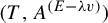
$(T,A^{(E-\unicode{x3bb} v)})$
. The behavior can be studied through the family of Schrödinger cocycles
$(T,A^{(E-\unicode{x3bb} v)})$
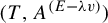 especially through the Lyapunov exponent
$L(E; \unicode{x3bb} )$
especially through the Lyapunov exponent
$L(E; \unicode{x3bb} )$
 . Kotani theory provides the relationship that the essential closure of the set of energies where the Lyapunov exponent is zero is equal to the absolutely continuous spectrum of
$\{H_{\omega }\}_{\omega \in \Omega }$
. Kotani theory provides the relationship that the essential closure of the set of energies where the Lyapunov exponent is zero is equal to the absolutely continuous spectrum of
$\{H_{\omega }\}_{\omega \in \Omega }$
 . As a consequence, if one has uniformly positive Lyapunov exponents, then the absolutely continuous spectrum is empty! Pairing this with a large deviation estimate, one has a strong indication of Anderson localization. For detailed accounts of using this method to conclude localization, we refer to [Reference Bourgain and Goldstein6–Reference Bucaj, Damanik, Fillman, Gerbuz, VandenBoom, Wang and Zhang8, Reference Jitomirskaya and Zhu27].
Results on positivity have been established in the iid setting by Furstenberg [Reference Furstenberg18], and also in the quasi-periodic setting by Sorets and Spencer [Reference Sorets and Spencer33] by extending methods from Herman [Reference Herman26] and Bourgain [Reference Bourgain4] for d-dimensional tori. For intermediate randomness, results are less satisfactory because reducing to a strongly mixing system leads to considerably more difficulty due to the absence of independence. In this paper, we focus on intermediate randomness through hyperbolic dynamics, which has two regimes: small and large coupling constants. For small coupling constants, Pastur and Figotin [Reference Pastur and Figotin29] developed methods that provided a necessary tool for Chulaevsky and Spencer [Reference Chulaevsky and Spencer10] to show positivity away from the center and edges of the spectrum for deterministic potentials with small coupling constants. Building upon this, Bourgain and Schlag [Reference Bourgain and Schlag7] established a large deviation theorem to achieve localization for almost every phase in the same spectral regime as Chulaevsky and Spencer [Reference Chulaevsky and Spencer10].
For large coupling, Bjerklöv [Reference Bjerklöv3] established positivity for circle endomorphisms, and Zhang and Li [Reference Zhang and Li38] extends the result to expanding toral automorphisms. Moreover, Bourgain and Bourgain-Chang [Reference Bourgain and Bourgain-Chang5] established positivity for any non-negative coupling, as long as one has sufficient hyperbolicity and
$C^1$
 non-constant potentials. Results in this regime have also been shown by Sadel and Baldes [Reference Sadel and Schulz-Baldes31], Damanik and Killip [Reference Damanik and Killip16], and Krüger [Reference Krüger28]. Recently, a more complete answer for hyperbolic base dynamics was given from Avila, Damanik, and Zhang [Reference Avila, Damanik and Zhang1]. They were able to show that for
$\alpha $
non-constant potentials. Results in this regime have also been shown by Sadel and Baldes [Reference Sadel and Schulz-Baldes31], Damanik and Killip [Reference Damanik and Killip16], and Krüger [Reference Krüger28]. Recently, a more complete answer for hyperbolic base dynamics was given from Avila, Damanik, and Zhang [Reference Avila, Damanik and Zhang1]. They were able to show that for
$\alpha $
 -Hölder continuous functions, the set
$\mathcal {Z} = \{E\in \mathbb {R}: L(E) = 0\}$
-Hölder continuous functions, the set
$\mathcal {Z} = \{E\in \mathbb {R}: L(E) = 0\}$
 is discrete and there exists a constant
$\unicode{x3bb} _0(v)$
is discrete and there exists a constant
$\unicode{x3bb} _0(v)$
 so that
$\mathcal {Z}$
so that
$\mathcal {Z}$
 is finite for all
$0 < \unicode{x3bb} < \unicode{x3bb} _0$
is finite for all
$0 < \unicode{x3bb} < \unicode{x3bb} _0$
 . Additionally, there is an open dense set
$\mathcal {O}^\alpha \subset C^\alpha (\mathbb {T}^d,\mathbb {R})$
. Additionally, there is an open dense set
$\mathcal {O}^\alpha \subset C^\alpha (\mathbb {T}^d,\mathbb {R})$
 such that one has uniformly positive Lyapunov exponents for all potentials in
$\mathcal {O}^\alpha $
such that one has uniformly positive Lyapunov exponents for all potentials in
$\mathcal {O}^\alpha $
 . For more general information on results of positive Lyapunov exponents, we refer to [Reference Wang and Zhang35].
There are many other interesting approaches to studying positivity, including understanding the topological structure of the spectrum, which was studied by Damanik and Fillman [Reference Damanik and Fillman13, Reference Damanik and Fillman14]. The two were able to show that for the doubling map and hyperbolic toral automorphisms with continuous sampling function, one has a connected essential spectrum. By using Kotani theory, one can return back to Lyapunov exponents and conclude positivity almost everywhere.
Another perspective is through Young’s [Reference Young37] method. Young studied the Lyapunov exponent for cocycles of the form

where R is a rotation matrix that rotates an amount depending on a function
$\phi _\epsilon : \mathbb {R}/\mathbb {Z} \rightarrow \mathbb {R}/2\pi \mathbb {Z}$
 . Young found that one has positive Lyapunov exponents as long as
$\phi _\epsilon $
. Young found that one has positive Lyapunov exponents as long as
$\phi _\epsilon $
 satisfies three conditions: compactly supported, monotone on the support, and whose derivative is positive and bounded away from zero. Damanik [Reference Damanik11, Problem 6] observed that it would be possible to show positive Lyapunov exponents for Schrödinger cocycles with the method used by Young. At the time, it was unclear how to apply it directly since the method required the cocycle to be of the form (2). Zhang showed that Schrödinger cocycles with sufficiently large coupling constants could be studied by defining a new cocycle that has a similar form as (2). The difference from (2) to Zhang’s setting is that the matrix entries
$\unicode{x3bb} $
satisfies three conditions: compactly supported, monotone on the support, and whose derivative is positive and bounded away from zero. Damanik [Reference Damanik11, Problem 6] observed that it would be possible to show positive Lyapunov exponents for Schrödinger cocycles with the method used by Young. At the time, it was unclear how to apply it directly since the method required the cocycle to be of the form (2). Zhang showed that Schrödinger cocycles with sufficiently large coupling constants could be studied by defining a new cocycle that has a similar form as (2). The difference from (2) to Zhang’s setting is that the matrix entries
$\unicode{x3bb} $
 are no longer constants, but functions. However, this can be dangerous as the functions may cancel the expanding effects of the base dynamics. One of the key observations was the function attached to the rotation matrix only needed to have monotonicity, and derivative positive and bounded away from zero. This led to Zhang’s result of positivity for potentials generated by the doubling map [Reference Zhang41].
This paper is a generalization of Zhang’s result by increasing the dimension. We do so by focusing on the setting where Arnold’s cat map T acts on
$\mathbb {T}^2$
 equipped with two-dimensional Lebesgue measure. We remark that we refer to
$[0,1)^2$
equipped with two-dimensional Lebesgue measure. We remark that we refer to
$[0,1)^2$
 as the fundamental domain of
$\mathbb {T}^2$
as the fundamental domain of
$\mathbb {T}^2$
 . From first observations, one should expect a geometric obstruction to be able to run an argument similar to Zhang. Young remarked that the method provided in [Reference Young37] should generalize by adjusting the conditions to depend on unstable foliations. We show that this adjustment on our potential is sufficient for the Schrödinger setting, which leads us to our main result.
Theorem 1. Let
$v\in C^1([0,1)^2, \mathbb {R})$
 be a bounded potential (examples of potentials are provided in §2) with directional derivative in the unstable direction positive and uniformly away from zero for all
$\omega \in [0,1)^2$
be a bounded potential (examples of potentials are provided in §2) with directional derivative in the unstable direction positive and uniformly away from zero for all
$\omega \in [0,1)^2$
 . Consider the family of Schrödinger operators as in (1) with Arnold’s cat map
$(\mathbb {T}^2, T, \mu )$
. Consider the family of Schrödinger operators as in (1) with Arnold’s cat map
$(\mathbb {T}^2, T, \mu )$
 , then there exists a
$C_0 = C_0(v)>0$
, then there exists a
$C_0 = C_0(v)>0$
 such that for any
$\unicode{x3bb}>0$
such that for any
$\unicode{x3bb}>0$
 , we have

To show this theorem, we emulate the framework provided in Zhang’s work. We briefly describe the steps and ideas from Zhang’s method:
-
(i) polar decomposition;
-
(ii) control the derivative from below of inductively defined functions $\theta _n$
 that are tracking the angle of
$\vec {e}_1$
under iterations of the cocycle;
that are tracking the angle of
$\vec {e}_1$
under iterations of the cocycle; -
(iii) count the number of discontinuities of $\theta _n$
and points in the domain such that the image under
$\theta _n$
is an element of
${\pi }/{2} + \pi \mathbb {Z}$
; -
(iv) control the measure of pre-images of $\delta $
-balls around each
${\pi }/{2}+ \pi \mathbb {Z}$
; -
(v) conclude positivity.


Step (i) provides the relation from Schrödinger cocycles to cocycles of the form of (2). Step (ii), plays two roles: monotonicity and a lower estimate on derivatives. Monotonicity combined with the counting of discontinuities leads to the counting process of elements in the domain with a
${\pi }/{2} + \pi \mathbb {Z}$
 image under
$\theta _n$
image under
$\theta _n$
 . With step (iii) attained, one finds that the pre-images of
$\delta $
. With step (iii) attained, one finds that the pre-images of
$\delta $
 -balls will be contained in a union
$\delta $
-balls will be contained in a union
$\delta $
 -balls around each element from step (iii). To control the measure, one uses the estimate from step (ii) combined with the mean value theorem. Finally, positivity is concluded by using Young’s argument.
The process described necessitates a one-dimensional space, so it is not immediately apparent to what space we should reduce. A natural approach would be to reduce to one-dimension by showing positivity on a leaf in the canonical unstable foliation, but therein lies an obstruction. A leaf crosses the fundamental domain infinitely often and each crossing produces a discontinuity. This leads step (iii) to an infinite set of discontinuities and points in the domain with a
${\pi }/{2}$
 image. This creates a complication in step (iv), as step (ii) uniformly controls the size of
$\delta $
image. This creates a complication in step (iv), as step (ii) uniformly controls the size of
$\delta $
 -balls and step (iii) controls the number that arise. Provided infinite points, the argument leads to an upper bound consisting of an infinite sum of a single number. Thus, one needs to control step (iii) from above by a finite number for the sum to have the ability to converge.
To overcome this obstacle, we introduce local unstable leaves
$W_z$
 , where
$z\in (0,1)$
, where
$z\in (0,1)$
 . (Local unstable leaves are defined rigorously in §2.) The initial purpose of the family of
$W_z$
. (Local unstable leaves are defined rigorously in §2.) The initial purpose of the family of
$W_z$
 is to reduce the two-dimensional problem to one dimension. This follows from Rohklin’s disintegration, which provides the relation that integration of
$\mathbb {T}^2$
is to reduce the two-dimensional problem to one dimension. This follows from Rohklin’s disintegration, which provides the relation that integration of
$\mathbb {T}^2$
 is equal to the double integral over z then the leaf
$W_z$
is equal to the double integral over z then the leaf
$W_z$
 . Thus, it suffices to show positivity on local unstable leaves then integrate to obtain an estimate on
$\mathbb {T}^2$
. Thus, it suffices to show positivity on local unstable leaves then integrate to obtain an estimate on
$\mathbb {T}^2$
 ! After reducing the dimension, we apply step (i) with the same argument, while step (ii) requires minor adjustments to account for directional derivatives. The second purpose for local unstable leaves is that it removes the challenge in step (iii), described in the preceding paragraph, since
$W_z$
! After reducing the dimension, we apply step (i) with the same argument, while step (ii) requires minor adjustments to account for directional derivatives. The second purpose for local unstable leaves is that it removes the challenge in step (iii), described in the preceding paragraph, since
$W_z$
 is finite and
$T^nW_z$
is finite and
$T^nW_z$
 always crosses the boundary of the fundamental domain finitely many times. With steps (ii) and (iii) combined, the estimate is well balanced to imply step (iv). Finally, we conclude step (v) on local unstable leaves using a similar argument to [Reference Young37, Reference Zhang41].
The upshot is that the argument is not restricted to Arnold’s cat map. In fact, the argument to prove positivity holds for any hyperbolic
$\mathrm {SL}(2,\mathbb {Z})$
 matrix! Let T represent any hyperbolic matrix action on
$\mathbb {T}^2$
matrix! Let T represent any hyperbolic matrix action on
$\mathbb {T}^2$
 and let
$\beta>1$
and let
$\beta>1$
 represent the largest eigenvalue. In this setting, one can define local unstable leaves in an analogous way to Arnold’s cat map. After defining the local unstable leaves, one swaps the eigenvalue of Arnold’s cat map with
$\beta $
represent the largest eigenvalue. In this setting, one can define local unstable leaves in an analogous way to Arnold’s cat map. After defining the local unstable leaves, one swaps the eigenvalue of Arnold’s cat map with
$\beta $
 for all proofs to conclude positivity. We formalize this exposition in a theorem.
Theorem 2. Consider any hyperbolic matrix in
$\mathrm {SL}(2,\mathbb {Z})$
 with eigenvalues
$\beta , \beta ^{-1}$
with eigenvalues
$\beta , \beta ^{-1}$
 , where
$|\beta |> 1$
, where
$|\beta |> 1$
 . If v is defined as in Theorem 1, then there exists a
$C_0 = C_0(v)>0$
. If v is defined as in Theorem 1, then there exists a
$C_0 = C_0(v)>0$
 such that for any
$\unicode{x3bb}> 0$
such that for any
$\unicode{x3bb}> 0$
 , we have

The remainder of the paper is organized as follows. Section 2 begins with preliminaries, examples of potentials, reduction via polar decomposition, reduction to local unstable leaves, and proof of Theorem 1 assuming positivity on local unstable leaves. Section 3 provides proofs to show positivity on local unstable leaves and follows an analogous structure to [Reference Zhang41]. Lastly, we include Appendix A, which summarizes the details of polar decomposition.
2 Preliminaries
We define the
$2$
 -torus as
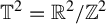
$\mathbb {T}^2 = \mathbb {R}^2/\mathbb {Z}^2$
-torus as
$\mathbb {T}^2 = \mathbb {R}^2/\mathbb {Z}^2$
 with fundamental domain
$[0,1)^2$
with fundamental domain
$[0,1)^2$
 . We equip
$\mathbb {T}^2$
. We equip
$\mathbb {T}^2$
 with Borel sigma-algebra and two-dimensional Lebesgue measure
$\mu $
with Borel sigma-algebra and two-dimensional Lebesgue measure
$\mu $
 . Define a linear map
$T:~\mathbb {R}^2 \rightarrow \mathbb {R}^2$
. Define a linear map
$T:~\mathbb {R}^2 \rightarrow \mathbb {R}^2$
 ,
,

and remark that T is invertible because

Moreover, abusing notation, the linear map induces a map
$T:\mathbb {T}^2 \rightarrow \mathbb {T}^2$
 ,
,

We refer to the measurable dynamical system
$(\mathbb {T}^2, T, \mu )$
 , described above, as Arnold’s cat map.
Consider Arnold’s cat map and the Schrödinger operators as in (1). Recall we are interested in the behavior of
$\psi $
 when
$H_\omega \psi = E \psi $
when
$H_\omega \psi = E \psi $
 for
$E\in \mathbb {R}$
for
$E\in \mathbb {R}$
 . For each energy
$E\in \mathbb {R}$
. For each energy
$E\in \mathbb {R}$
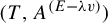
 , we define an associated Schrödinger cocycle
$(T,A^{(E-\unicode{x3bb} v)})$
, we define an associated Schrödinger cocycle
$(T,A^{(E-\unicode{x3bb} v)})$
 . The cocycle map
$A^{(E-\unicode{x3bb} v)}: \mathbb {T}^2 \rightarrow \mathrm {SL}(2,\mathbb {R})$
. The cocycle map
$A^{(E-\unicode{x3bb} v)}: \mathbb {T}^2 \rightarrow \mathrm {SL}(2,\mathbb {R})$
 is defined as

The iterates of the cocycle map are written as

and have a direct relation to solutions of the eigenvalue equation, since
$\psi $
 is a solution if and only if

The Lyapunov exponent is defined as

where the existence of the limit follows by subadditivity. Moreover, since
$\mu $
 is ergodic, we can apply Kingman’s subadditive ergodic theorem on each
$E\in \mathbb {R}$
is ergodic, we can apply Kingman’s subadditive ergodic theorem on each
$E\in \mathbb {R}$
 to obtain

For information on why the Lyapunov exponent is interesting, general theory, and specific classes on Schrödinger operators, we highly recommend respectively [Reference Damanik and Fillman12, Reference Damanik and Fillman15, Reference Wilkinson36].
To reduce the dimension of the problem, we introduce a family of local unstable leaves, which is a line segment in the unstable direction. To formalize this, recall that for Arnold’s cat map, the largest eigenvalue and associated unit eigenvector is

respectively.
For each
$z\in (0,1)$
 , we define

and denote the graph of
$f_z$
 as
$\Gamma (f_z)$
as
$\Gamma (f_z)$
 . For each
$z\in (0,1)$
. For each
$z\in (0,1)$
 , a local unstable leaf is defined as

Geometric picture representing the local unstable leaves (family of parallel lines) and the line parameterizing the leaves (diagonal line that descends from the top-left to the bottom-right corner of the fundamental domain) (color online).

See Figure 1. We remark that as z increases from
$0$
 to
$1$
to
$1$
 , the parameterization of the family of local unstable leaves follows the diagonal line that descends from the top left to bottom right corner of the fundamental domain. Moreover, for each
$z\in (0,1)$
, the parameterization of the family of local unstable leaves follows the diagonal line that descends from the top left to bottom right corner of the fundamental domain. Moreover, for each
$z\in (0,1)$
 , the local unstable leaf is the unique line segment in
$[0,1)^2$
, the local unstable leaf is the unique line segment in
$[0,1)^2$
 containing the element
$(z,1-z)$
containing the element
$(z,1-z)$
 with slope
$({\sqrt {5}-1})/{2}$
with slope
$({\sqrt {5}-1})/{2}$
 . Lastly, we let
$\ell _z$
. Lastly, we let
$\ell _z$
 denote the length of
$W_z$
denote the length of
$W_z$
 , then a direct computation shows that
$\ell _z\in (0, \sqrt {({5-\sqrt {5}})/{2}}]$
, then a direct computation shows that
$\ell _z\in (0, \sqrt {({5-\sqrt {5}})/{2}}]$
 .
.
Throughout the paper, we let
$c,C$
 represent universal constants, where c is some small constant and C is some large constant. These constants only depend on the measurable potential
$v:\mathbb {T}^2\rightarrow \mathbb {R}$
represent universal constants, where c is some small constant and C is some large constant. These constants only depend on the measurable potential
$v:\mathbb {T}^2\rightarrow \mathbb {R}$
 that satisfies the following:
-
(i) v is bounded;
-
(ii) $v\in C^1([0,1)^2, \mathbb {R})$
; -
(iii) for all $\omega \in \mathbb {T}^2$
, the directional derivative of v in the unstable direction uniformly away from zero. That is, for all
$\omega \in \mathbb {T}^2$
, one has
$|D_{\vec {u}}v(\omega )|> c$
.




Without loss of generality, we may assume that the potential satisfies
$D_{\vec {u}}v(\omega )> c$
 , as the argument for when
$D_{\vec {u}}v(\omega ) < -c$
, as the argument for when
$D_{\vec {u}}v(\omega ) < -c$
 is completely analogous. Moreover, after translation and normalization, we may assume that
$0\leq v(\omega ) \leq 1$
is completely analogous. Moreover, after translation and normalization, we may assume that
$0\leq v(\omega ) \leq 1$
 for all
$\omega \in [0,1)^2$
for all
$\omega \in [0,1)^2$
 .
.
To establish notation, let
$J_v(\omega )$
 denote the Jacobian of v evaluated at
$\omega $
denote the Jacobian of v evaluated at
$\omega $
 . For clarity, when taking partial derivatives, we will write
$\partial [v\circ T](\omega )$
. For clarity, when taking partial derivatives, we will write
$\partial [v\circ T](\omega )$
 to emphasize that the chain rule has not been applied and we drop the brackets,
$\partial v(T\omega )$
to emphasize that the chain rule has not been applied and we drop the brackets,
$\partial v(T\omega )$
 , to denote the partial derivative of v evaluated at
$T\omega $
, to denote the partial derivative of v evaluated at
$T\omega $
 .
.
We explore some enjoyable examples of such potentials.
Example 1. Fix an
$n\in \mathbb {N}$
 and define a polynomial in two variables

where
$a_k,b_k \in \mathbb {R}\geq 0$
 and
$a_1 \neq 0$
and
$a_1 \neq 0$
 or
$b_1\neq 0$
or
$b_1\neq 0$
 . Then,
$v\in C^1([0,1)^2)$
. Then,
$v\in C^1([0,1)^2)$
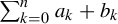
 and is bounded above by
$\sum _{k=0}^n a_k + b_k$
and is bounded above by
$\sum _{k=0}^n a_k + b_k$
 . We directly compute the Jacobian of v evaluated at
$\omega \in [0,1)^2$
. We directly compute the Jacobian of v evaluated at
$\omega \in [0,1)^2$
 :
:

The directional derivative with respect to the unstable direction is

Therefore,
$D_{\vec {u}}v(\omega )> c$
 for any
$\omega \in [0,1)^2$
for any
$\omega \in [0,1)^2$
 .
.
Example 2. Consider an exponential function defined as

which is contained in
$C^1([0,1)^2)$
 and bounded by
$e^2$
and bounded by
$e^2$
 . The Jacobian of v evaluated at
$\omega \in [0,1)^2$
. The Jacobian of v evaluated at
$\omega \in [0,1)^2$
 is
is

and the directional derivative in the unstable direction is

Example 3. Consider the logarithm function defined as

which is in
$C^1([0,1)^2)$
 and bounded by
$\log (3)$
and bounded by
$\log (3)$
 . Computing the Jacobian of v evaluated at
$\omega \in [0,1)^2$
. Computing the Jacobian of v evaluated at
$\omega \in [0,1)^2$
 , we find

and it follows that

The polar decomposition motivates us to define a new cocycle of a similar form to (2). See Appendix A for more details, as we provide a brief summary here. To begin, we let
$t = {E}/{\unicode{x3bb} }$
 and
$t\in \mathcal {I} = [-1, 2]$
and
$t\in \mathcal {I} = [-1, 2]$
 . Define functions
$r,g: \mathbb {T}^2\times \mathcal {I} \rightarrow \mathbb {R}$
. Define functions
$r,g: \mathbb {T}^2\times \mathcal {I} \rightarrow \mathbb {R}$
 as
as

Since v is bounded, we have

We define a new matrix

where

and
$\theta (\omega ,t)$
 is
is

Let
$\theta _0 = \theta (\omega ,t)$
 and for every
$n\in \mathbb {N}$
and for every
$n\in \mathbb {N}$
 , we define

Lastly, we denote the Lyapunov exponent for the cocycle
$(T, A(\cdot , t, \unicode{x3bb} ))$
 as
$\tilde {L}(t;\unicode{x3bb} )$
as
$\tilde {L}(t;\unicode{x3bb} )$
 .
.
We remark that
$A = D\circ T$
 , which is used for the convenience of excluding
$T^{-1}$
, which is used for the convenience of excluding
$T^{-1}$
 from the function
$\theta $
from the function
$\theta $
 , see Appendix A for the definition of D. The Lyapunov exponent is T-invariant so the estimates found for A also hold for D. In the construction of D, we found that for each
$E\in \mathbb {R}$
, see Appendix A for the definition of D. The Lyapunov exponent is T-invariant so the estimates found for A also hold for D. In the construction of D, we found that for each
$E\in \mathbb {R}$
 ,
$A^{(E-\unicode{x3bb} v)}$
,
$A^{(E-\unicode{x3bb} v)}$
 is conjugate to
$\Lambda (\cdot , t)\cdot O(\cdot , t)$
is conjugate to
$\Lambda (\cdot , t)\cdot O(\cdot , t)$
 by a piecewise
$C^1$
by a piecewise
$C^1$
 and bounded map
$S(\cdot , t): \mathbb {T}^2 \rightarrow \mathrm {SL}(2,\mathbb {R})$
and bounded map
$S(\cdot , t): \mathbb {T}^2 \rightarrow \mathrm {SL}(2,\mathbb {R})$
 . That is,

See Appendix A for more details on
$\Lambda (\cdot , t), O(\cdot , t)$
 , and
$S(\cdot , t)$
, and
$S(\cdot , t)$
 . For simplicity, we may drop the notation emphasizing the dependence of t for the remaining parts of the paper, as all estimates in the future will be uniform in t. The conjugation map S is
$\log $
. For simplicity, we may drop the notation emphasizing the dependence of t for the remaining parts of the paper, as all estimates in the future will be uniform in t. The conjugation map S is
$\log $
 -integrable in the sense that

which preserves the Lyapunov exponent. Also, as
$\unicode{x3bb} $
 tends to infinity, the conjugated matrix
$\Lambda \cdot O$
tends to infinity, the conjugated matrix
$\Lambda \cdot O$
 approaches D in the
$C^1$
approaches D in the
$C^1$
 -topology, see Lemma 4 in Appendix A. By proving that
$\tilde {L}(t;\unicode{x3bb} )$
-topology, see Lemma 4 in Appendix A. By proving that
$\tilde {L}(t;\unicode{x3bb} )$
 is positive, we may pass positivity and the lower estimates to the cocycle
$(T,\Lambda \cdot O)$
is positive, we may pass positivity and the lower estimates to the cocycle
$(T,\Lambda \cdot O)$
 by using T-invariance and the stability of our argument under
$C^1$
by using T-invariance and the stability of our argument under
$C^1$
 perturbations. Therefore, the positivity and lower estimates for
$(T,\Lambda \cdot O)$
perturbations. Therefore, the positivity and lower estimates for
$(T,\Lambda \cdot O)$
 implies the same holds for
$(T,A^{(E-\unicode{x3bb} v)})$
implies the same holds for
$(T,A^{(E-\unicode{x3bb} v)})$
 . Thus, it suffices to show positivity of
$\tilde {L}(t;\unicode{x3bb} )$
. Thus, it suffices to show positivity of
$\tilde {L}(t;\unicode{x3bb} )$
 to show positivity for
$L(E;\unicode{x3bb} )$
to show positivity for
$L(E;\unicode{x3bb} )$
 , see [Reference Zhang39] for the argument on why Theorem 3 implies Theorem 1. For additional details on polar decomposition, we refer to Appendix A, [Reference Zhang39], and [Reference Zhang41, Appendix A].
Theorem 3. For v as in Theorem 1, there exists a
$C_0 = C_0(v)>0$
 such that for any
$\unicode{x3bb}>0$
such that for any
$\unicode{x3bb}>0$
 , we have

There is a subtlety between Theorems 1 and 3, as t is contained in a compact interval, but Theorem 1 holds for all energies
$E\in \mathbb {R}$
 . For sufficiently large
$\unicode{x3bb} $
. For sufficiently large
$\unicode{x3bb} $
 and any energy
${E\in \mathbb {R}\setminus [-\unicode{x3bb} ,2\unicode{x3bb} ]}$
and any energy
${E\in \mathbb {R}\setminus [-\unicode{x3bb} ,2\unicode{x3bb} ]}$
 , the cocycle
$A^{(E-\unicode{x3bb} v)}$
, the cocycle
$A^{(E-\unicode{x3bb} v)}$
 is uniformly hyperbolic. This can be directly shown by checking the uniform exponential growth condition, which is equivalent to uniform hyperbolicity. Moreover, the exponential growth factor is of size
$\unicode{x3bb} $
is uniformly hyperbolic. This can be directly shown by checking the uniform exponential growth condition, which is equivalent to uniform hyperbolicity. Moreover, the exponential growth factor is of size
$\unicode{x3bb} $
 , which implies that the Lyapunov exponent is uniformly bounded away from
$\log \unicode{x3bb} - C_0$
, which implies that the Lyapunov exponent is uniformly bounded away from
$\log \unicode{x3bb} - C_0$
 . Hence, Theorem 1 holds for all energies
$E\in \mathbb {R}$
. Hence, Theorem 1 holds for all energies
$E\in \mathbb {R}$
 . For information on the equivalent conditions of uniform hyperbolicity, we refer to [Reference Zhang40].
To prove Theorem 3, recall that given a measurable map
$\pi :X\rightarrow Y$
 , a disintegration of a measure
$\mu $
, a disintegration of a measure
$\mu $
 with respect to the fibers of
$\pi $
with respect to the fibers of
$\pi $
 is a family of probability measures
$\{m_y\}_{y\in Y}$
is a family of probability measures
$\{m_y\}_{y\in Y}$
 such that:
-
(1) $m_{y}(\pi ^{-1}(y)) = 1$
for
$\pi _*\mu $
almost every
$y\in Y$
; -
(2) given any measurable set $E\subset X$
, $$ \begin{align*}\mu(E) = \int m_{y}(E)\,d(\pi_*\mu).\end{align*} $$



The family of probability measures exists by Rohklin’s disintegration theorem, see [Reference Rokhlin30, Reference Viana34].
One can construct a measurable map
$\pi : [0,1)^2 \rightarrow (0,1)$
 such that
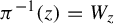
$\pi ^{-1}(z) = W_z$
such that
$\pi ^{-1}(z) = W_z$
 for every
$z\in (0,1)$
for every
$z\in (0,1)$
 . The map
$\pi $
. The map
$\pi $
 is defined to project
$W_z$
is defined to project
$W_z$
 onto the line
$y = 1-x$
onto the line
$y = 1-x$
 restricted to the fundamental domain with normalized length, see Figure 1. Applying Rohklin’s disintegration, we attain a family of probability measures
$\{m_z\}_{z\in (0,1)}$
restricted to the fundamental domain with normalized length, see Figure 1. Applying Rohklin’s disintegration, we attain a family of probability measures
$\{m_z\}_{z\in (0,1)}$
 , where each
$m_z$
, where each
$m_z$
 is a normalized Lebesgue measure on
$W_z$
is a normalized Lebesgue measure on
$W_z$
 . Moreover, for any
$g\in L^1(\mu )$
. Moreover, for any
$g\in L^1(\mu )$
 ,
,

where m is a normalized Lebesgue measure on the graph of
$y=1-x$
 restricted to the fundamental domain. Applying (9) on
$({1}/{n})\log \|A_n(\omega )\|\in L^1(\mu )$
restricted to the fundamental domain. Applying (9) on
$({1}/{n})\log \|A_n(\omega )\|\in L^1(\mu )$
 provides the equality

for every
$n\in \mathbb {N}$
 . Denoting the Lyapunov exponent on
$W_z$
. Denoting the Lyapunov exponent on
$W_z$
 as
$\tilde {L}(t;\unicode{x3bb} , z)$
as
$\tilde {L}(t;\unicode{x3bb} , z)$
 , we have the following proposition.
Proposition 1. There exists a
$C_0 = C_0(v)>0$
 such that for any
$\unicode{x3bb}> 0, z\in (0,1)$
such that for any
$\unicode{x3bb}> 0, z\in (0,1)$
 ,
,

for all
$t\in \mathcal {I}$
 .
.
This proposition’s main utility is that it proves Theorem 3.
Proof of Theorem 3.
For
$n\in \mathbb {N}, z\in (0,1)$
 , define
$g_n(\omega ) = ({1}/{n})\log \|A_n(\omega )\|$
, define
$g_n(\omega ) = ({1}/{n})\log \|A_n(\omega )\|$
 and
$f_n(z) = \int _{W_z} g_n(\omega )\, dm_z(\omega )$
and
$f_n(z) = \int _{W_z} g_n(\omega )\, dm_z(\omega )$
 . Notice that

and by definition of
$\tilde {L}(t;\unicode{x3bb} , z)$
 ,
$f_n(z) \rightarrow \tilde {L}(t;\unicode{x3bb} , z)$
,
$f_n(z) \rightarrow \tilde {L}(t;\unicode{x3bb} , z)$
 as
$n\rightarrow \infty $
as
$n\rightarrow \infty $
 . By Rohklin’s disintegration, we must have
$m_z(W_z) = 1$
. By Rohklin’s disintegration, we must have
$m_z(W_z) = 1$
 , so
, so

Remark
$\log \|A\|_\infty \in L^1(\mu )$
 , so applying Lebesgue dominated convergence theorem, (9), and Proposition 1, we attain

3 Proof of theorems
To show positive Lyapunov exponents, we use the methods in [Reference Zhang41] to show on each
$W_z$
 , one has positive Lyapunov exponents. To begin, we must control the directional derivative of
$D_{\vec {u}}\theta _n$
, one has positive Lyapunov exponents. To begin, we must control the directional derivative of
$D_{\vec {u}}\theta _n$
 uniformly from below.
Lemma 1. For any
$t\in \mathcal {I}$
 ,
,

for all
$n\in \mathbb {Z}_{\geq 0}$
 and
$\omega \in \mathbb {T}^2$
and
$\omega \in \mathbb {T}^2$
 , where
$\theta _n$
, where
$\theta _n$
 is differentiable.
Proof. Consider
$n=0$
 and let
$\omega \in \mathbb {T}^2$
and let
$\omega \in \mathbb {T}^2$
 ,
,

Assume for induction, (10) holds for some n, then we show that (10) holds for
$n+1$
 . A computation gives

which implies

Directly computing
$\partial _{\omega _1}$
 , we find


The estimates (12), (13), and (14) also hold for
$\partial _{\omega _2}$
 by replacing
$\partial _{\omega _1}$
by replacing
$\partial _{\omega _1}$
 with
$\partial _{\omega _2}$
with
$\partial _{\omega _2}$
 everywhere. Define

Combining (11) and (12), (13), and (14) for both partials, one obtains

Let
$h(\omega ) = \unicode{x3bb} ^2g(T^{n+1}\omega )\cot \theta _{n}(\omega )$
 , then for any
$\omega \in \mathbb {T}^2$
, then for any
$\omega \in \mathbb {T}^2$
 ,
,

If
$\omega \in \mathbb {T}^2$
 satisfies
$|g(T^{n+1}\omega )\cot \theta _{n}(\omega )|<C\unicode{x3bb} ^{-3/2}$
satisfies
$|g(T^{n+1}\omega )\cot \theta _{n}(\omega )|<C\unicode{x3bb} ^{-3/2}$
 , then

In this case, by equality (15) and applying (16), (17), one can conclude (10).

However, if
$\omega \in \mathbb {T}^2$
 satisfies
$|g(T^{n+1}\omega )\cot \theta _{n}(\omega )|>c\unicode{x3bb} ^{-3/2}$
satisfies
$|g(T^{n+1}\omega )\cot \theta _{n}(\omega )|>c\unicode{x3bb} ^{-3/2}$
 , then

Also, for any
$\omega \in \mathbb {T}^2$
 ,
,

Similar to the previous case, by applying (18) and (19) onto (15), we obtain

By chain rule on
$J_{v\circ T^{n+1}}$
 , we obtain


which is (10).
Lemma 2. Let
$\mathcal {D}^{\prime }_{n,z}, \mathcal {D}_{n,z}$
 be the set of discontinuities for
$\theta \circ T_n|_{W_z}$
be the set of discontinuities for
$\theta \circ T_n|_{W_z}$
 and
$\theta _n|_{W_z}$
and
$\theta _n|_{W_z}$
 , respectively. Let
$\mathrm{Card}(S)$
, respectively. Let
$\mathrm{Card}(S)$
 denote the cardinality of a set S. Then,


for any
$n\in \mathbb {Z}_{\geq 0}$
 and
$z\in (0,1)$
and
$z\in (0,1)$
 .
.
Proof. The discontinuities of

restricted to
$W_z$
 is equal to the set of discontinuities for
$v\circ T^n$
is equal to the set of discontinuities for
$v\circ T^n$
 . By our assumptions on v, the discontinuities occur when the graph of
$T^nW_z$
. By our assumptions on v, the discontinuities occur when the graph of
$T^nW_z$
 intersects the boundary of the fundamental domain. Thus, it suffices to bound the number of times this occurs from above.
Concretely, consider any
$n\in \mathbb {N}$
 and recall
$\ell _z\in (0, \sqrt {({5-\sqrt {5}})/{2}}]$
and recall
$\ell _z\in (0, \sqrt {({5-\sqrt {5}})/{2}}]$
 is the length of the line segment
$W_z$
is the length of the line segment
$W_z$
 . Iterating
$W_z$
. Iterating
$W_z$
 under
$T^n$
under
$T^n$
 stretches the length by a factor of
$\alpha ^n$
stretches the length by a factor of
$\alpha ^n$
 , which leads to
$T^nW_z$
, which leads to
$T^nW_z$
 having length
$\alpha ^n \ell _z$
having length
$\alpha ^n \ell _z$
 . By monotonicity of
$\theta \circ T^n|_{W_z}$
. By monotonicity of
$\theta \circ T^n|_{W_z}$
 , the graph
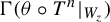
$\Gamma (\theta \circ T^n|_{W_z})$
, the graph
$\Gamma (\theta \circ T^n|_{W_z})$
 may only intersect horizontal lines
$y = k$
may only intersect horizontal lines
$y = k$
 and vertical lines
$x = k$
and vertical lines
$x = k$
 at most once per
$k\in \mathbb {N}$
at most once per
$k\in \mathbb {N}$
 . With the length of
$T^nW_z$
. With the length of
$T^nW_z$
 being
$\alpha ^n \ell _z$
being
$\alpha ^n \ell _z$
 , one finds there are at most
$\alpha ^n\ell _z + 1$
, one finds there are at most
$\alpha ^n\ell _z + 1$
 many times
$T^nW_z$
many times
$T^nW_z$
 intersects a horizontal line and similarly for vertical lines. Thus, the number of times
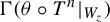
$\Gamma (\theta \circ T^n|_{W_z})$
intersects a horizontal line and similarly for vertical lines. Thus, the number of times
$\Gamma (\theta \circ T^n|_{W_z})$
 crosses the fundamental domain is at most
$2\alpha ^n\ell _z + 2$
crosses the fundamental domain is at most
$2\alpha ^n\ell _z + 2$
 , which is bounded above by
$\alpha ^{n+2}$
, which is bounded above by
$\alpha ^{n+2}$
 . Consequently,

which is (22).
To show (23), consider
$n=0$
 and notice that
$\mathcal {D}_{0,z}= \mathcal {D}^{\prime }_{0,z}$
and notice that
$\mathcal {D}_{0,z}= \mathcal {D}^{\prime }_{0,z}$
 , since
$\theta _0 = \theta $
, since
$\theta _0 = \theta $
 . Assume that (23) holds for some
$n\in \mathbb {N}$
. Assume that (23) holds for some
$n\in \mathbb {N}$
 , and observe that
$g\circ T^{n+1}|_{W_z}$
, and observe that
$g\circ T^{n+1}|_{W_z}$
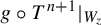 and
$\theta \circ T^{n+1}|_{W_z}$
and
$\theta \circ T^{n+1}|_{W_z}$
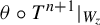 have the same set of discontinuities,
$\mathcal {D}^{\prime }_{n+1,z}$
have the same set of discontinuities,
$\mathcal {D}^{\prime }_{n+1,z}$
 , since both have a dependency on v. However,

has discontinuities
$\mathcal {D}_{n,z}$
 and
$\mathcal {D}^{\prime }_{n+1,z}$
and
$\mathcal {D}^{\prime }_{n+1,z}$
 due to the dependence on g and
$\theta _n$
due to the dependence on g and
$\theta _n$
 . Hence, the set of discontinuities of
$\theta _{n+1}|_{W_z}$
. Hence, the set of discontinuities of
$\theta _{n+1}|_{W_z}$
 satisfies the containment
$\mathcal {D}_{n+1,z} \subset \mathcal {D}^{\prime }_{n+1,z}\cup \mathcal {D}_{n,z}$
satisfies the containment
$\mathcal {D}_{n+1,z} \subset \mathcal {D}^{\prime }_{n+1,z}\cup \mathcal {D}_{n,z}$
 . By induction, (23) holds for any
$n\in \mathbb {Z}_{\geq 0}$
. By induction, (23) holds for any
$n\in \mathbb {Z}_{\geq 0}$
 .
.
Remark 1. With Lemmas 1 and 2, we have that
$\theta _n|_{W_z}$
 is piecewise
$C^1$
is piecewise
$C^1$
 and monotone. Moreover, in the proof of Lemma 2, we can additionally add two more points to
$\mathcal {D}^{\prime }_{n,z}$
and monotone. Moreover, in the proof of Lemma 2, we can additionally add two more points to
$\mathcal {D}^{\prime }_{n,z}$
 , since
$2\ell _z\alpha ^n + 4 < \alpha ^{n+2}$
, since
$2\ell _z\alpha ^n + 4 < \alpha ^{n+2}$
 for every
$n\in \mathbb {Z}_{\geq 0}$
for every
$n\in \mathbb {Z}_{\geq 0}$
 . Thus, the bound in both (22) and (23) holds with the additional points.
Lemma 3. For each
$z\in (0,1)$
 , we define

Then,

for all
$n\in \mathbb {N}$
 and
$z\in (0,1)$
and
$z\in (0,1)$
 .
.
Proof. Consider any
$z\in (0,1)$
 and restrict to
$W_z$
and restrict to
$W_z$
 . When
$n=0$
. When
$n=0$
 , notice that

By the assumption
$D_{\vec {u}}v> c$
 , the above can only occur at one
$\omega \in W_z$
, the above can only occur at one
$\omega \in W_z$
 . Assume for some
$n\in \mathbb {N}$
. Assume for some
$n\in \mathbb {N}$
 that (24) holds. Observe that

and recall, by Lemma 2, we have
$\mathrm{Card}(\mathcal {D}_{n+1,z})<\sum _{j=0}^{n+2} \alpha ^{j+1}$
 discontinuities for
$\theta _{n+1}|_{W_z}$
discontinuities for
$\theta _{n+1}|_{W_z}$
 . By Remark 1, we know that
$k := \mathrm{Card}(\mathcal {D}_{n+1,z}) + 2$
. By Remark 1, we know that
$k := \mathrm{Card}(\mathcal {D}_{n+1,z}) + 2$
 is bounded above by
$\sum _{j=0}^{n+2} \alpha ^{j+1}$
is bounded above by
$\sum _{j=0}^{n+2} \alpha ^{j+1}$
 . We may label the discontinuities and the end points of
$W_z$
. We may label the discontinuities and the end points of
$W_z$
 , two additional points, as
$\{\omega _j\}_{j=1}^k$
, two additional points, as
$\{\omega _j\}_{j=1}^k$
 . By the isometry
$i:W_z \rightarrow [0, \ell _z)$
. By the isometry
$i:W_z \rightarrow [0, \ell _z)$
 , we may further assume that the points are ordered:

For each
$1\leq j \leq k - 1$
 , we define
$I_j = [\omega _j, \omega _{j+1})$
, we define
$I_j = [\omega _j, \omega _{j+1})$
 and it is apparent that
$W_z = \bigcup _{j=1}^{k-1} I_j$
and it is apparent that
$W_z = \bigcup _{j=1}^{k-1} I_j$
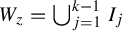 . For each
$T^nI_j$
. For each
$T^nI_j$
 , there exists some
$\ell \in (0,1)$
, there exists some
$\ell \in (0,1)$
 such that
$T^nI_j\subset W_\ell $
such that
$T^nI_j\subset W_\ell $
 . Consider any
$I_j$
. Consider any
$I_j$
 , then

By Lemma 2, it follows that
$\theta _{n+1}$
 is
$C^1$
is
$C^1$
 and monotone on
$I_j$
and monotone on
$I_j$
 . Moreover, for
$\omega \in W_z$
. Moreover, for
$\omega \in W_z$
 , one has
$c < \theta (\omega ) < \pi - c$
, one has
$c < \theta (\omega ) < \pi - c$
 . These facts imply

By direct computation,

and we have shown Lemma 3.
As a consequence of Lemmas 1 and 3, we can bound the measure of the elements in the pre-image of the set of
$\delta $
 -balls around
${\pi }/{2} + \pi \mathbb {Z}$
-balls around
${\pi }/{2} + \pi \mathbb {Z}$
 .
.
Corollary 1. Let
$\delta>0$
 and
$\|\cdot \|_{\mathbb {R}\mathbb {P}^1}$
and
$\|\cdot \|_{\mathbb {R}\mathbb {P}^1}$
 represent the distance to the closest
$\pi \mathbb {Z}$
represent the distance to the closest
$\pi \mathbb {Z}$
 point. Define

Then,

for all
$n\in \mathbb {N}$
 and
$z\in (0,1)$
and
$z\in (0,1)$
 .
.
Proof. By Lemma 3, there are at most
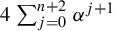
$\sum _{j=0}^{n+2} \alpha ^{j+1}$
 many elements in
$W_z$
many elements in
$W_z$
 that have image under
$\theta _n$
that have image under
$\theta _n$
 inside the set
${\pi }/{2} + \pi \mathbb {Z}$
inside the set
${\pi }/{2} + \pi \mathbb {Z}$
 , so the number of connected components is bounded above by
$4\sum _{j=0}^{n+2} \alpha ^{j+1}$
, so the number of connected components is bounded above by
$4\sum _{j=0}^{n+2} \alpha ^{j+1}$
 . By Lemma 1,
$\theta _n$
. By Lemma 1,
$\theta _n$
 passes through a distance of
$2\delta $
passes through a distance of
$2\delta $
 at a speed of at least
$c\alpha ^n$
at a speed of at least
$c\alpha ^n$
 , so the pre-image of a
$\delta $
, so the pre-image of a
$\delta $
 -ball has measure bounded above by
$C({2\delta }/{\alpha ^n})$
-ball has measure bounded above by
$C({2\delta }/{\alpha ^n})$
 . Using these facts paired with
${1}/{\alpha }< 1$
. Using these facts paired with
${1}/{\alpha }< 1$
 , we attain the following estimate:

We are now ready to prove Proposition 1. The argument follows an identical structure as [Reference Zhang41], which followed similar arguments in [Reference Young37]. For completeness, we include the proof.
Proof of Proposition 1.
Let
$\vec {e}_1, \vec {e}_2$
 represent the standard basis of
$\mathbb {R}^2$
represent the standard basis of
$\mathbb {R}^2$
 . Then, observe

and existence follows from Oseledet’s multiplicative ergodic theorem. Define

so we can rewrite

by (6). Let
$\omega \in W_z$
 , then define for
$n\geq 0$
, then define for
$n\geq 0$
 ,
,

Rewriting, we find

The previous line implies

and by definition of
$\theta _n(\omega )$
 ,
,

Directly, one finds

Inductively, one finds

It follows that

and then,

From (25), it suffices to find a lower bound of
$\int _{W_z} \log |\!\cos \theta _j(\omega )|\,dm_z(\omega )$
 . Fix any
$k \in ~\{0,\dots , n-1\}$
. Fix any
$k \in ~\{0,\dots , n-1\}$
 and define for all
$i\in \mathbb {N}$
and define for all
$i\in \mathbb {N}$
 ,
,

By Corollary 1,

for all
$i\in \mathbb {N}$
 . A computation gives

Consider

It follows that

Picking
$\delta = \tfrac 13$
 and putting everything together,

for any
$k\in \{0,1\dots , n-1\}$
 . Thus, it follows that

for all
$n\in \mathbb {N}$
 , which implies

This completes the proof of Proposition 1, which proves Theorem 3 and hence Theorem 1.
A Appendix. Polar decomposition of Schrödinger cocycle
In this section, we focus on discussing why Theorem 1 can be reduced to Theorem 3. To do so, we recall that given a matrix
$M\in \mathrm {SL}(2,\mathbb {R})$
 , we can use singular value decomposition (SVD) on M. Consequently,

where
$S_1,S_2\in \mathrm {SO}(2,\mathbb {R})$
 ,
$S_2^t$
,
$S_2^t$
 is the transpose of
$S_2$
is the transpose of
$S_2$
 , and
$\Lambda $
, and
$\Lambda $
 has the form
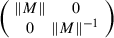
$\Big(\begin {smallmatrix} \|M\| & 0\\ 0 & \|M\|^{-1} \end {smallmatrix}\Big)$
has the form
$\Big(\begin {smallmatrix} \|M\| & 0\\ 0 & \|M\|^{-1} \end {smallmatrix}\Big)$
 . Moreover, for
$M\in C^r(\mathbb {T}^2, \mathrm {SL}(2,\mathbb {R}))$
. Moreover, for
$M\in C^r(\mathbb {T}^2, \mathrm {SL}(2,\mathbb {R}))$
 ,
$r\geq 1$
,
$r\geq 1$
 , we can let
$S(\omega ) = S_1(\omega )S_2(\omega )$
, we can let
$S(\omega ) = S_1(\omega )S_2(\omega )$
 and
$O(\omega )=~S_2^t(\omega ) (S_1S_2)(T^{-1}\omega )$
and
$O(\omega )=~S_2^t(\omega ) (S_1S_2)(T^{-1}\omega )$
 . It follows by (A.1) that

By [Reference Zhang39, Lemma 10],
$S_1,S_2, \Lambda $
 are also
$C^r$
are also
$C^r$
 , as long as
$M(\omega )\notin \mathrm {SO}(2,\mathbb {R})$
, as long as
$M(\omega )\notin \mathrm {SO}(2,\mathbb {R})$
 for all
$\omega \in ~\mathbb {T}^2$
for all
$\omega \in ~\mathbb {T}^2$
 . Consequently, the conjugacy of M and
$\Lambda \cdot O$
. Consequently, the conjugacy of M and
$\Lambda \cdot O$
 is
$C^r$
is
$C^r$
 , which implies that the Lyapunov exponent for the cocycles
$(T,M)$
, which implies that the Lyapunov exponent for the cocycles
$(T,M)$
 and
$(T, \Lambda \cdot O)$
and
$(T, \Lambda \cdot O)$
 are equal.
In our setting, we will show that
$A^{(E-\unicode{x3bb} v)}$
 has a
$\mathrm {SL}(2,\mathbb {R})$
has a
$\mathrm {SL}(2,\mathbb {R})$
 conjugacy that is piecewise
$C^1$
conjugacy that is piecewise
$C^1$
 and bounded, which is naturally
$\log $
and bounded, which is naturally
$\log $
 -integrable. This provides the advantage to study the Lyapunov exponent with the cocycle alternating between rotation and stretching, which is a similar form to (2). The rotation matrix O is quite complicated, so by letting
$\unicode{x3bb} $
-integrable. This provides the advantage to study the Lyapunov exponent with the cocycle alternating between rotation and stretching, which is a similar form to (2). The rotation matrix O is quite complicated, so by letting
$\unicode{x3bb} $
 tend to infinity, we can define a new matrix that is close to
$\Lambda \cdot O$
tend to infinity, we can define a new matrix that is close to
$\Lambda \cdot O$
 in
$C^1$
in
$C^1$
 norm. The limiting matrix has a much simpler rotation on which to run analysis, which defines the cocycle for which we will show positivity. Our argument is stable under
$C^1$
norm. The limiting matrix has a much simpler rotation on which to run analysis, which defines the cocycle for which we will show positivity. Our argument is stable under
$C^1$
 perturbations, as the essential part of the argument is the
$C^1$
perturbations, as the essential part of the argument is the
$C^1$
 -shape of
$\theta $
-shape of
$\theta $
 and g. Thus, after obtaining positivity with the limiting cocycle, we pass positivity and the lower estimates to
$\Lambda \cdot O$
and g. Thus, after obtaining positivity with the limiting cocycle, we pass positivity and the lower estimates to
$\Lambda \cdot O$
 . We summarize the discussion with the following lemma.
Lemma 4. Consider Arnold’s cat map
$(\mathbb {T}^2,T,\mu )$
 and the associated Schrödinger cocycle

with
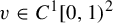
$v\in C^1[0,1)^2$
 and bounded. For each
$E\in \mathbb {R}$
and bounded. For each
$E\in \mathbb {R}$
 , the Schrödinger cocycle
$A^{(E-\unicode{x3bb} v)}$
, the Schrödinger cocycle
$A^{(E-\unicode{x3bb} v)}$
 is conjugate to
$\Lambda \cdot O$
is conjugate to
$\Lambda \cdot O$
 , where
$\Lambda $
, where
$\Lambda $
 is a diagonal matrix and O is a rotation matrix, by a piecewise
$C^1$
is a diagonal matrix and O is a rotation matrix, by a piecewise
$C^1$
 and bounded map
$S:\mathbb {T}^2 \rightarrow \mathrm {SL}(2,\mathbb {R})$
and bounded map
$S:\mathbb {T}^2 \rightarrow \mathrm {SL}(2,\mathbb {R})$
 , as in (A.2). Moreover, for any compact interval
$\mathcal {J} \ni t$
, as in (A.2). Moreover, for any compact interval
$\mathcal {J} \ni t$
 , as
$\unicode{x3bb} \rightarrow \infty $
, as
$\unicode{x3bb} \rightarrow \infty $
 , then
$\Lambda \cdot O$
, then
$\Lambda \cdot O$
 converges to

in
$C^1([0,1)^2\times \mathcal {J}, \mathrm {SL}(2,\mathbb {R}))$
 , where
$t = {E}/{\unicode{x3bb} }$
, where
$t = {E}/{\unicode{x3bb} }$
 . In the above,
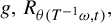
$g, R_{\theta (T^{-1}\omega , t)},$
. In the above,
$g, R_{\theta (T^{-1}\omega , t)},$
 and
$\theta $
and
$\theta $
 are defined as (5), (7), and (8), respectively.
Proof. Define
$r: \mathbb {T}^2\times \mathbb {R} \rightarrow \mathbb {R}$
 as
as

which is an element of
$C^1([0,1)^2\times \mathbb {R}, \mathbb {R})$
 . We conjugate
$A^{(E-\unicode{x3bb} v)}$
. We conjugate
$A^{(E-\unicode{x3bb} v)}$
 with
with

which leads to

The conjugation by P is
$C^1$
 , since P is a constant matrix.
Next, we compute the SVD of B, which will lead to a piecewise
$C^1$
 conjugacy due to the discontinuities of r along the boundary of the fundamental domain of
$\mathbb {T}^2$
conjugacy due to the discontinuities of r along the boundary of the fundamental domain of
$\mathbb {T}^2$
 . To begin, we compute
$B^tB$
. To begin, we compute
$B^tB$
 , then we can directly find that the largest eigenvalue of
$B^tB$
, then we can directly find that the largest eigenvalue of
$B^tB$
 is
is

Defining

the largest singular value of B is
$\sqrt {\alpha }$
 , so
$\|B\| = \unicode{x3bb} \sqrt {{\beta }/{2}}$
, so
$\|B\| = \unicode{x3bb} \sqrt {{\beta }/{2}}$
 . Thus, we define

Solving for the eigenvectors of
$B^tB$
 and normalizing, we can define

where

With this, we may define the map
$S = P^{-1}S_1S_2:\mathbb {T}^2 \rightarrow \mathrm {SL}(2,\mathbb {R})$
 , where
$S_1$
, where
$S_1$
 is defined as
$S_1 = B(\sqrt {B^tB})^{-1}$
is defined as
$S_1 = B(\sqrt {B^tB})^{-1}$
 . Remark that
$\sqrt {B^tB}$
. Remark that
$\sqrt {B^tB}$
 is invertible, since B is invertible. The dependence on
$B,S_2$
is invertible, since B is invertible. The dependence on
$B,S_2$
 , and P implies that for each t, S is piecewise
$C^1$
, and P implies that for each t, S is piecewise
$C^1$
 and bounded. From the singular value decomposition of B and the definition of S, one has that for each
$E\in \mathbb {R}$
and bounded. From the singular value decomposition of B and the definition of S, one has that for each
$E\in \mathbb {R}$
 ,
,

which is (A.2).
For the latter half of the lemma, we define

and compute the upper left entry of O:

Consider any compact interval
$\mathcal {J} \ni t$
 . Letting
$\unicode{x3bb} \rightarrow \infty $
. Letting
$\unicode{x3bb} \rightarrow \infty $
 , for any
$\omega \in \mathbb {T}^2, t\in \mathcal {J}$
, for any
$\omega \in \mathbb {T}^2, t\in \mathcal {J}$
 , we find

and hence,

where convergence is with respect to
$C^1([0,1)^2\times \mathcal {J}, \mathbb {R})$
 . Thus, for sufficiently large
$\unicode{x3bb} $
. Thus, for sufficiently large
$\unicode{x3bb} $
 ,
$O_{11}(\omega , t, \unicode{x3bb} )$
,
$O_{11}(\omega , t, \unicode{x3bb} )$
 can be replaced with
$({r(T^{-1}\omega )})/{\sqrt {r^2(T^{-1}\omega )+1}}$
can be replaced with
$({r(T^{-1}\omega )})/{\sqrt {r^2(T^{-1}\omega )+1}}$
 since they are close in
$C^1$
since they are close in
$C^1$
 norm. Therefore, for large enough
$\unicode{x3bb} $
norm. Therefore, for large enough
$\unicode{x3bb} $
 , the cocycle
$\Lambda \cdot O$
, the cocycle
$\Lambda \cdot O$
 tends to

where

Acknowledgements
Thanks are due to my advisor Zhenghe Zhang for providing me with the problem to explore positive Lyapunov exponents for the cat map, the helpful discussions of background and ideas, the comments to improve my writing, and the endless support. I would like to also thank Alex Tao and Agnieszka Zelerowicz for the numerous insightful conversations and support provided. Also, thanks to Jake Fillman for bringing several additional references to my attention to add to this paper. Finally, I want to emphasize that words cannot describe how grateful I am to the referee. The referee has provided an enormous amount of insightful feedback consisting of: related references, improvements to the overall structure, readability, and clarity of the paper.


 Open access

