Implications

Breeding and management strategies that produce more robust animals will increase production efficiency in a sustainable way, and thereby contribute to meeting the challenges of food security for the expanding human population and climate change. However, no consensus exists in the definition of robustness nor in ways to measure it. This study describes why a proper characterisation of robustness must take into account its multiple components, trade-offs between them, and dynamic elements such as the rates of response to, and recovery from, environmental perturbations. This then provides an improved basis for including robustness in management strategies and breeding programmes.

A generic robustness definition to facilitate its use in practise

Including robustness in future breeding and management strategies implies being able to measure and quantify it but no single, simple, useful measure of robustness currently exists. This is largely because robustness is a complex trait which relates to a whole biological system. Typically, measures of animal performance are only one part of a biological system. For example, there are numerous studies that have investigated the ability of cows to maintain milk production when feed quality is reduced (e.g. Horan et al., Reference Horan, Faverdin, Delaby, Rath and Dillon2006; Beerda et al., Reference Beerda, Ouweltjes, Šebek, Windig and Veerkamp2007), and these can be used to estimate the environmental sensitivity of milk production via the slope of change in milk production relative to the change in environment quality (usually referred to as a reaction norm (Lewontin, Reference Lewontin1974)). However, to equate environmental sensitivity of a single trait such as milk yield with robustness could be considered meaningless; milk production or indeed any other single trait, is only one part of the entire biological system whose aim is to ensure a return on investment in reproductive effort, that is, to produce viable offspring. This biological system includes other important components such as use of body reserves as well as maternal behaviour. Selecting only on one component, such as milk yield in dairy cows, has been shown to reduce robustness, with unfavourable consequences on reproduction and health (Pryce et al., Reference Pryce, Coffey, Brotherstone and Woolliams2002; Berry et al., Reference Berry, Bermingham, Good and More2011). It is therefore important to emphasise this notion of a biological system when considering robustness. Indeed, the closest that one can come to a single measure of farm animal robustness is productive longevity because it is an integration over time of an animal’s cumulative ability to overcome the environmental challenges it has faced throughout life. However, productive longevity has limitations as a robustness measure (apart from it being an end-point measure) as it should only be used to compare animals kept in identical environments. Differences in productive longevity between environments will be heavily influenced by the level of challenge experienced in the different local production environments, for example, farmer culling rules and environment harshness. A zero-challenge environment will facilitate long productive lifespan even in animals with zero robustness. Further, productive lifespan does not provide any information on the relative importance of different components of robustness.

The general consensus is that robustness of a given system (level n) is the consequence of multiple components at lower levels of organisation (n−1, n−2, etc.), and that a given level of robustness can be achieved by different combinations of its component mechanisms (Kitano, Reference Kitano2004; Bateson and Gluckman, Reference Bateson and Gluckman2011). In general terms, the system can be a herd, an individual animal, a life function, an organ or a cell but if the robustness measure is to be of long-term value it must capture the integrity of the response to an environmental perturbation at the system level. Several reviews exist that discuss the robustness of biological systems within which the animal is a component (e.g. ten Napel et al., Reference ten Napel, van der Veen, Oosting and Groot Koerkamp2011), but also where the biological system is, in fact, a subsystem within the animal (Kitano, Reference Kitano2004; Taff and Vitousek, Reference Taff and Vitousek2016). For the purpose of this review we focus on the level of the animal. At the level of the animal, we can define robustness as:

This broad definition meets the previously stated requirement of considering the entire biological system, and is largely equivalent to other recent definitions of robustness in the animal sciences (Knap, Reference Knap2009; Amer, Reference Amer2012). However, it should be noted that this definition can, in principle, be applied to other levels of organisation of biological systems with only minor changes in wording, for example, at the level of the cell (Kitano, Reference Kitano2004) or at the level of the farm (ten Napel et al., Reference ten Napel, van der Veen, Oosting and Groot Koerkamp2011) or species (Martin and Wiebe, Reference Martin and Wiebe2004). At first sight, the definition of robustness appears to be too vague a definition to be of any use but it focusses attention on the key elements of robustness. These are discussed with the aim of illustrating how consideration of these elements can generate approaches to quantify robustness.

Key elements of robustness: favouring future ability to reproduce

The aforementioned definition of robustness explicitly attributes a purpose to animal-level robustness, which is ‘to favour its future ability to reproduce’. This should be seen in terms of the animal, male or female, maintaining the capacity to eventually continue disseminating its genes, either whilst the environment imposes constraints or in a less constraining future environment. Thus, the future ability to reproduce includes growth (needed to attain sexual maturity) and surviving until future reproductive opportunities, as well as successfully reproducing. It implies that robustness contributes directly to animal fitness; indeed the above definition of robustness is equally valid in both natural and artificial selection contexts. This is a useful property considering the emergence of the agro-ecology approach in which there is no longer a clear dichotomy between populations that are under natural selection and artificial selection. Instead, all species within an ecosystem are considered to be on a continuum of degree of management and thus affected, to varying degrees, by both artificial and natural selection.

With respect to selection, ‘future ability to reproduce’ often maps onto probability of surviving to breed, or breed again, or in other words achieving productive longevity, that is, avoiding death whether that be natural death or culling within a managed population. Some robustness components such as disease resistance will have a high value in both managed and natural environments, while others will be more environment dependent. Rabbits exist in both natural and farmed environments, often in close geographic proximity. For wild rabbits, the ability to cope with food shortage and to avoid predation are clearly important robustness components, whereas they are of little robustness value for farmed rabbits. On the other hand, the ability to avoid being culled for poor performance is an important characteristic in farmed rabbits but of lesser value to the wild rabbit. In general, robustness can be considered in the same way as a multi-trait index commonly used in breeding, made up of multiple components that are appropriately weighted according to their fitness value in a given environment and production system. This view of robustness is useful as it makes explicit the concept of relative contributions of different robustness components, and provides a framework within which to evaluate the consequences of trade-offs between robustness components that consider the environment in which the animal (or its progeny) exist. The association of robustness with fitness and selection is supported by evidence that the ability to cope with environmental challenge is heritable (Mirkena et al., Reference Mirkena, Duguma, Haile, Tibbo, Okeyo, Wurzinger and Sölkner2011; Drangsholt et al., Reference Drangsholt, Damsgård and Olesen2014).

The implications for quantifying robustness are that there is no single measure of robustness but rather that robustness is the combination of multiple and interacting component mechanisms. Although these mechanisms are all inherent traits of the animal, their relative value is context dependent. This context encompasses both the prevailing environment (e.g. strong heat stress tolerance is of greater value in environments where high temperatures occur) and the prevailing selection pressure. Favouring future ability to reproduce implies avoiding premature culling due to failure to meet the selection criteria of the farmer or the natural pressures imposed by the environment. Thus, the question of which robustness components are the most important to measure requires a clear vision of the environmental and selection context in which the animals will live and produce.

With respect to characterising the environmental context, it is important to identify what are major challenge types (nutritional availability, thermal stress, disease pressure, etc.) in the prevailing environment, and within this it is useful to consider the environment as having two components. The first is general ‘harshness’ of the environment which includes the nutritional conditions, the constraints imposed by the farming system, and other stable factors such as the average meteorological conditions of the location. The second component of the environment relates to the frequency and intensity of environmental perturbations. Some environments are harsh but relatively stable and some environments are on average good but with frequent perturbations. As will become clear in the following sections, coping with general harshness relies on different component mechanisms of robustness than those needed to cope with perturbations. The former are usually referred to as adaptation mechanisms (Mirkena et al., Reference Mirkena, Duguma, Haile, Tibbo, Okeyo, Wurzinger and Sölkner2011) whereas the latter, which result in a dynamic pattern of response and recovery, are usually referred to as animal resilience mechanisms.

Key elements of robustness: ‘the various things the animal needs to do’

The ‘various things’ influencing robustness are those that maximise the future ability to reproduce, or in other words minimise the risk of the animal being culled or dying, in the prevailing environment. For instance, Sewalem et al. (Reference Sewalem, Miglior, Kistemaker, Sullivan and Van Doormaal2008) documented a greater culling risk in Canadian dairy cows that experienced calving difficulty or reduced reproductive performance. This means that a robust Canadian cow should calve without assistance and have good reproductive performance. In their definition of a robust dairy cow in New Zealand, Pryce et al. (Reference Pryce, Harris, Bryant and Montgomerie2009) used characteristics related to calving, fertility, body size, foraging ability and resistance to disease. De Hollander et al. (Reference De Hollander, Knol, Heuven and van Grevenhof2015) described longevity relative to culling reasons in sows. Calus et al. (Reference Calus, Berry, Banos, de Haas and Veerkamp2013) dissected robustness in dairy cattle into workability, health, persistency, fertility, mobility, fitness. As culling criteria are specific to each species, production context and environmental constraints, it is not easy to give a definitive list of specific traits that constitute robustness.

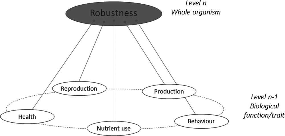
As shown in Figure 1, if one considers the functional components of robustness, then some commonality arises. Each functional component has, of course, associated behavioural, physiological and morphological traits making the phenotyping of the functional components possible. For instance, the New Zealand and Irish robust grazing cow has a good resource acquisition function relying on behaviour (exploration), morphology (small body size to not damage pastures soil) and physiology (digestive efficiency). Conversely, any given trait may be associated with different functions. For instance, low aggressiveness contributes to social interactions (easy handling by the farmer) but also to health status (fewer injuries from handling).

Figure 1 A schematic representation of the ‘various things’ operating at underlying levels (n−1) that combine to build robustness at the level (n) of the animal.

Globally, a robust farm animal is an animal:

• ∙ That produces in accordance with farmer expectations. This production function implies both quantitative aspects (quantity of product, weight or number of weaned offspring) and quality aspects (fat concentration in milk or meat, fibre diameter of wool).

• ∙ That makes maximum use of the available nutritional resource, which includes both resource acquisition and nutrient utilisation abilities. It implies traits related to feed intake (exploration behaviour for grazing; feeding behaviour), digestion and metabolism (digestive efficiency, absence of metabolic disorders, fibre degradation).

• ∙ That matches with the physical characteristics of its environment (temperature, humidity, surface). It implies thermoregulation capacity (heat or cold stress) and also locomotion aspects (hoof, body size).

• ∙ That is able to reproduce well and regularly, or at least at the interval desired by the production system. This implies temporal traits (interval between parturitions, days post-parturition to service) and qualitative traits (heat expression, easy of birth, semen quality).

• ∙ That has a good health status, or in other words, disease resistance or resilience. This implies all the traits related to immune status and their temporal variability.

• ∙ That fits well with the behavioural environment, including good social interactions, both with the farmer and contemporaries. This implies traits such as temperament (easy handling), milkability, parental care, aggressiveness and training abilities.

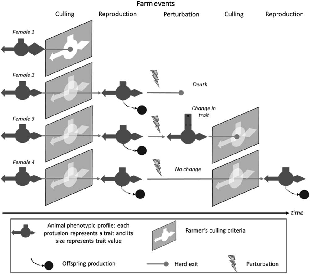
As shown in Figure 2, a robust animal is also one that responds appropriately to the prevailing environment, including not only perturbations but also the limits set by farm management. There is clearly a time dimension to robustness which is discussed in the next section. The multivariate aspect of robustness is increasingly being considered in breeding programmes. More recent selection indexes in dairy cattle now include non-productive, functional, traits (Egger-Danner et al., Reference Egger-Danner, Cole, Pryce, Gengler, Heringstad, Bradley and Stock2015). However, these broader indexes do not per se imply that robustness of farmed livestock will improve. Robustness may still be selected against when, for example, considering traits like short-term efficiency where the fastest gains are made by maximising the production component at the expense of ‘non-productive’ functions (Puillet et al., Reference Puillet, Réale and Friggens2016). The ultimate examples of ignoring the need to maintain associated functions are in breeding programmes that have selected aggressively for increased meat production, for example, in young broilers, with relatively little direct consideration of the unfavourable consequences of this selection strategy for rapid growth on the ability of adult birds to reproduce (Nestor et al., Reference Nestor, Noble, Zhu and moritsu1996). The trade-off between milk production and reproduction in dairy cows has been extensively reviewed elsewhere (Berry et al., Reference Berry, Friggens, Lucy and Roche2016).

Figure 2 Schematic representation the interaction between animal types and the prevailing environment, illustrated by the trajectories of four animal types in the herd, which give different levels of robustness depending on farm events. In this representation, different animal traits are portrayed as geometric protrusions (rectangle, arrow, diamond) and the farmers culling criteria as ‘keyholes’ into which the animals must fit if they are to progress. Animal 1 does not pass the first culling event: she does not have the traits values that match with farmer’s expectations. Animals 2 to 4 pass through this first selection gate and stay in the herd where they breed and produce offspring. The next event is an environmental perturbation (e.g. a health challenge). Animal 2 does not survive the challenge. Animal 3 copes with the challenge but with a change in the value of one trait. Animal 4 copes with the challenge without changing traits values. At the second culling event, animal 3 does not pass the selection gate because of the change in a trait value. Animal 4 pass through the selection gate imposed by farmer’s selection criteria and produces offspring at the next breeding event.

Manipulating robustness through the net effect of multiple components requires an understanding of the interconnectedness among these components. Defining the various functional components of robustness is only the first step. The next step is to characterise how and why the components are interlinked. One approach is to explore the underlying mechanisms, for example, associating production with reproduction (Boer et al., Reference Boer, Apri, Molenaar, Stötzel, Veerkamp and Woelders2012). This is extremely useful for linking key robustness mechanisms to gene expression and genomics. From the applied point of view, this is crucial if we are to develop biomarkers of (different types of) robustness. However, it is becoming clearer that making the link between molecular-level phenotypic measures and the higher-level functions they underpin is not trivial. From a systemic point of view, robustness derives from the interplay between mechanisms that individually may seem to counteract, or where several alternative mechanisms exist to achieve the same functionality (i.e. there is redundancy). Moreover, different mechanisms can confer a range of properties such as flexibility, plasticity, rigidity and modularity, on different parts of the system (Kitano, Reference Kitano2004; Bateson and Gluckman, Reference Bateson and Gluckman2011). Finding reliable biomarkers for robustness is thus a complex process requiring not only detailed knowledge of different mechanisms but also an understanding of their roles within the robustness architecture. Nonetheless, the interaction among functions and associated traits can be usefully considered at a higher level, in terms of resource allocation.

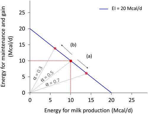
Resource allocation is the process of partitioning a limited quantity of resource among activities or structures. It implies that the resource used for one activity cannot be used for another activity or process. Because of resource allocation, an animal cannot maximise every biological function expression (Stearns, Reference Stearns1992), and thus we should not expect animals to be robust to all types of environmental perturbations. Investing in robustness to thermal stress does not necessarily imply robustness to pathogen load. For the same quantity of available resource, an increased investment in one function necessarily implies a reduced investment in another function. Figure 3 depicts this concept for energy investment in milk production and in maintenance plus weight gain. The negative association between traits such as these is termed a trade-off. Although the correlation between traits is antagonistic, trade-offs are usually an adaptive response (i.e. beneficial) to a change in environment. Understanding these trade-offs is essential to predicting robustness and the interactions among the ‘various things’ of our definition.

Figure 3 Example of allocation of energy intake (EI, Mcal/day) between milk production and non-productive functions (defined here as maintenance and weight gain) for a dairy cow that consumes 20 Mcal/day. Energy for milk production=α.EI and energy for maintenance and gain=(1−α).EI. The blue line represents all the potential values for two traits depending on the allocation coefficient α. The negative slope reflects the trade-off. The red dot in the middle corresponds to an animal with an allocation coefficient at 0.5, enabling to cover maintenance (assumed at 10 Mcal/day) and produces 13.5 kg of milk (at 0.74 Mcal/kg). With the same level of EI, increasing production level (arrow (a)) corresponds to an increase of allocation coefficient (0.7) and a decrease in the energy allocated for maintenance and gain. Conversely, increasing maintenance and gain (arrow (b)) corresponds to a decrease of allocation coefficient (0.3) and a decrease in milk production.

Changing resource allocation, that is, making a trade-off among functions, is not the only response possible. The animal may be able to change its resource acquisition. Resource acquisition is the process of gathering the different resources required to survive and reproduce (e.g. energy, nutrients, water). In the context of livestock species, resource acquisition is often simplified to feed intake or energy intake. In some constraining situations (e.g. decreased feed quality) the animal may be able to increase acquisition to counteract the constraint, in others (e.g. heat stress) it may be that reducing acquisition without changing resource allocation is an appropriate response. For instance, Figure 4 clearly illustrates that both milk production and energy for maintenance and gain can be increased with an increase in acquisition (25 Mcal/day) or decreased with a reduction in acquisition (15 Mcal/day). Both potential responses exist with constant allocation (i.e. 0.5 in this example).

Figure 4 Example of allocation of energy intake (EI, Mcal/day) between milk production and non-productive functions (defined here as maintenance and weight gain) for a dairy cow with three different levels of intake and the same level of allocation between milk production and non-productive functions.

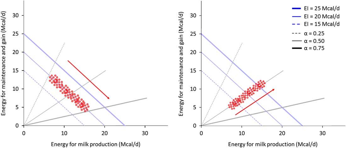
When studying allocation responses to different environments it is important to also consider what is happening to acquisition. The relative variability of these two components in a population can conceal some trade-offs; Figure 5 illustrates this phenomenon. On the left panel, animals exhibit a large variability in allocation (between black lines) while having a small variation in acquisition (along the blue line). Non-productive functions and milk appear to be negatively correlated. On the right panel, animals exhibit small variability in allocation but a high variability in acquisition. Milk and non-productive functions appear positively correlated. The trade-off between milk and non-productive functions exists in both examples as energy is always allocated between these two functions. Yet, the observed correlation between them depends on the variability of acquisition relative to allocation (van Noordwijk and De Jong, Reference van Noordwijk and De Jong1986). However, the relative value for robustness of greater variability in allocation or acquisition can only be determined in the broader context of the prevailing environment and the production goals (Douhard et al., Reference Douhard, Friggens, Amer and Tichit2014; Puillet et al., Reference Puillet, Réale and Friggens2016).

Figure 5 Example of observed associations between two traits linked by resource allocation within two contrasted populations of animals, for two traits that are in a trade-off within animal. The animals in the left panel population have a high variability in resource allocation (allocation coefficient between 0.25 and 0.75) and a low variability in resource acquisition (energy intake (EI) around 20 Mcal/day). The two traits, energy for maintenance and gain and energy for milk production, appear to be negatively correlated and it seems not possible to increase milk production without decreasing maintenance and gain. The animals in the right panel population have a high variability in resource acquisition (between 15 and 25 Mcal/day) and a low variability in allocation (coefficient around 0.5). The energy for maintenance and gain and the energy for milk production appear to be positively correlated and it seems possible to increase both milk production and maintenance and gain. This example shows that even if allocation still exists at animal level (and therefore shapes the relation among traits), the population level can conceal the relation among traits if allocation and acquisition are not evaluated together.

The resource acquisition and allocation approach provides a useful framework for interpreting observed G×E interactions in a holistic manner (Savietto et al., Reference Savietto, Friggens and Pascual2015). It has also proved useful for predicting G×E interactions in livestock systems (Douhard et al., Reference Douhard, Friggens, Amer and Tichit2014; Puillet et al., Reference Puillet, Réale and Friggens2016). From the perspective of quantifying the relative importance of allocation and acquisition to animal robustness, we need to go a step further and include the costs associated with both processes. Altering resource acquisition or allocation is costly because it requires adaptive mechanisms. Change in acquisition usually implies changes in the digestive structure and absorptive mechanisms (i.e. cost of gastrointestinal and splanchnic tissues). Change in allocation implies channelling resources through different metabolic pathways, and maintaining the mechanisms that allow metabolic flexibility (e.g. multiple pathways). Thus, the benefits of changing acquisition and/or allocation to cope with a particular environment need to be weighed up against the associated costs. Typically, extreme combinations are not viable and there is usually an optimum for a given environment. The concepts involved in building cost-benefit models of resource allocation have been summarised by Friggens and Van der Waaij (Reference Friggens and van der Waaij2009). Recent advances in modelling of multi-criteria cost-benefits can be applied to identify the viable allocation combinations, and to further identify the optimum combinations.

The key issue with respect to choosing which components of robustness to measure is to be clear on the use to which they will be put. If the purpose is to identify biomarkers of (aspects of) robustness such as may be useful for molecular phenotyping or genotyping, then the measurements should focus on the physiological mechanisms underlying robustness, and the components of robustness are thus viewed in terms of these mechanisms (e.g. the role of key intermediaries such as cortisol). However, if the purpose of measuring robustness is in order to quantify the extent to which animals can adapt to limiting conditions then the measurements should focus on the life functions involved. When resources are limited it is important to be able to quantify the trade-off between these functions. When not limited, the animal’s capacity to increase resource acquisition also comes into play.

Key elements of robustness: ‘carry on doing’

The preceding section described a key aspect of robustness, namely achieving an appropriate, adaptive, balance between different life functions relative to prevailing conditions, and hence an optimal allocation of resources to these functions. An additional key aspect of robustness is the ability to adapt to environmental perturbations, and thus be resilient. This ability allows the animal to improve its chances of passing relatively unaffected through a period of challenging conditions, that is, to ‘carry on doing the various things that the animal needs to do to favour its future ability to reproduce’. Multiple mechanisms of this resilience capacity exist, each of which operate on different timescales, and time is the key element for understanding them. Indeed, it seems implausible to evaluate robustness without considering its dynamic, resilience, properties.

Adapting to short-term, acute, challenges

Animals can respond extremely rapidly to environmental challenges through behavioural and physiological changes, and these are often linked to the ‘fight or flight’ reaction. Such responses can occur in seconds and provoke changes in, for example, cortisol that persist for an hour or two (Canario et al., Reference Canario, Mignon-Grasteau, Dupont-Nivet and Phocas2013). As these innate survival responses are ubiquitous, they are rarely considered as components of robustness. However, using environmental challenges that persisted for 2 h, significant between-animal variability in rates of response and rates of recovery post-challenge have been documented (Larsen et al., Reference Larsen, Røntved, Ingvartsen, Vels and Bjerring2010; Sadoul et al., Reference Sadoul, Leguen, Colson, Friggens and Prunet2015a). Sadoul et al. (Reference Sadoul, Leguen, Colson, Friggens and Prunet2015a) compared two isogenic lines of rainbow trout and documented significant differences between lines in cortisol response to a confinement challenge, and evidence of two different coping strategies favouring either behavioural or physiological responses, suggesting a genetic component to these short-term adaptive mechanisms.

Several recent studies have attempted to quantify the inter-individual variability in response to short-term nutritional challenges lasting 2 to 4 days, tracking performance and blood metabolites of animals before, during and after a shift from a standard feed to a very poor quality feed (Bjerre-Harpøth et al., Reference Bjerre-Harpøth, Friggens, Thorup, Larsen, Ingvartsen and Moyes2012; Friggens et al., Reference Friggens, Duvaux-Ponter, Etienne, Mary-Huard and Schmidely2016). Both studies documented inter-animal variability in responses in dry matter intake and milk production which was largely related to pre-challenge levels. However, as shown in Figure 6, considerably more variability existed in the underlying components such as milk protein, and some blood metabolites, which suggests that the same overall response can be achieved through different combinations of underlying mechanisms, a well-recognised feature of robustness and adaptive capacity (Lee et al., Reference Lee, Atkins and Sladek2009). These results on short-term challenges suggest that it may be possible to select animals according to which adaptive mechanisms they favour. If, as seems likely, different mechanisms are better suited to different types of challenge, for example, heat stress v. nutritional stress, then this may be, especially in the era of genomics, a useful tool to select animals according to the type of challenge which is most likely to occur in the future.

Figure 6 Example of individual animal trajectories before, during and after an environmental perturbation for (a) milk yield and (b) plasma glucose in 16 dairy goats. The perturbation, replacement of the normal feed by straw only commenced on day 0 and lasted until day 2, full details given in Friggens et al. (Reference Friggens and van der Waaij2016) (reproduced with permission).

In the above studies, the nutritional challenge also provoked a negative energy balance, that is, a mobilisation of energy from the body reserves to buffer the shortfall in nutritional supply. The use of the body as a buffer, is a well-recognised role of body lipid, and to a much lesser extent body protein and bone mineral reserves. This type of body tissue mobilisation is a response to prevailing environmental conditions and, for the purpose of understanding adaptive mechanisms, should not be confused with the long-term patterns of body reserve change that are described below.

Life trajectories of resource allocation

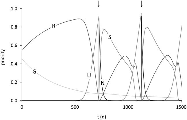
The optimum allocation of resources between life functions will change as the animal moves through different life stages. In most species, growth is the major resource-requiring function in early life, whereas reproduction (including lactation) becomes the major resource drain in adult life. Thus, the resource allocation considerations are incomplete unless their time dynamic is considered. As shown in Figure 7, it is useful to consider life trajectories of resource allocation under normal conditions, that is, those the animal evolved to deal with (Martin and Sauvant, Reference Martin and Sauvant2010). This provides a biologically logical baseline against which to evaluate an animal’s ability to cope with environmental perturbations. Clearly, if these relative priorities of resource allocation are altered, for instance, by genetic selection, in such a way as to divert resources away from those life functions that are key to robustness such as the accumulation of body reserves and development of immunocompetence, then robustness will be compromised. Furthermore, the evidence that the genetic expression of key robustness elements such as body reserve levels varies through life (Friggens et al., Reference Friggens, Berg, Theilgaard, Korsgaard, Ingvartsen, Løvendahl and Jensen2007) strongly suggests that robustness itself varies across life stages. This raises important questions, the robust animal has a greater probability of an increased (productive) lifespan because of it being less likely to succumb to any given stressor but at what cost? Are there sensitive time-points in the life trajectory? What are the combined effects of the cumulative environments (stresses, diseases, etc.) during development of the young animal on the subsequent performance of adult genotypes? What are the relative contributions of robustness and innate longevity to functional longevity? It would be extremely useful to be able to quantify this, in particular, with respect to arguments about lifetime efficiency. Currently, we have an insufficient understanding of these issues.

Figure 7 Trajectories of the priorities for growth (G), balance of body reserves (R), ensuring survival of the unborn calf (U), ensuring survival of the newborn calf (N) and ensuring survival of the suckling calf (S) over 1500 days of life in the model of Martin and Sauvant (Reference Mathur, Herrero-Medrano, Alexandri, Knol, ten Napel, Rashidi and Mulder2010). The arrows indicate parturition times of two successive reproductive cycles. Priority for ageing is close to 0 at this stage of the lifespan. Reproduced with permission.

Timing as key component of robustness

A key adaptation with respect to ‘carry on doing’, that is, maintaining the ability to reproduce in the future, is the ability to shut down and postpone high-risk processes when the environmental conditions become harsh. Here the animal is making a trade-off but using time as the resource. A ubiquitous feature of female mammals is to cease oestrus cycling or prolong the postpartum anoestrus period when the nutritional conditions are too risky. This has been observed in all farmed species. The available evidence indicates that environmentally driven mobilisation of body tissue reserves (i.e. negative energy balance) is not only an energetic response but also has signal value to the female as an index of the quality of the current nutritional environment. Further, it also appears that the size of body lipid reserves provides a signal, probably via leptin and other adipokines, of the animal’s ability to cope with any future nutritional challenge. Figure 8 shows that both of these factors delay return to oestrus cycling in beef cattle (Wright et al., Reference Wright, Rhind, Whyte and Smith1992; De La Torre et al., Reference De La Torre, Recoules, Blanc, Ortigues-Marty, D’Hour and Agabriel2015). This timing component of robustness, as evidenced by length of postpartum anoestrus, exhibits heritable variation between individuals, and has been negatively associated with increasing production levels (Royal et al., Reference Royal, Pryce, Woolliams and Flint2002).

Figure 8 The effect of body fatness on the relationship between days to resumption of luteal activity and energy mobilisation measured as change in condition score. Thin cows (open symbols) have longer days to resumption of cyclicity than fat cows (solid symbols) and the delay to recover cyclicity after calving is strongly reduced in thin cows when they experience positive energy balance after calving. Drawn from data of Wright et al. (Reference Yatoo, Kumar, Dimri and Sharma1992) (■, □) and data from the experiment described by De la Torre et al. (Reference De La Torre, Recoules, Blanc, Ortigues-Marty, D’Hour and Agabriel2015) (▲, ∆).

This time-related aspect of robustness has important implications for measuring it. It is clear that single time-point measurements to quantify robustness are of limited value because they do not permit measurement of responses to (and recovery from) environmental perturbations. The exception being single measurements of the accumulated consequence of a good (or bad) adaptive capacity. Good examples of such a measurements are productive longevity and lifetime efficiency. However, the counterpoint to this limitation is that repeated measurements have a high potential to facilitate quantification of the animal’s ability to cope with environmental challenges. Thus, we should be able to quantify differences in adaptive capacity from the kind of data that are increasingly becoming available with the deployment of automated monitoring technology on farm (Rutten et al., Reference Rutten, Velthuis, Steeneveld and Hogeveen2013). The capability to obtain near-continuous measurement of performance at low cost (milk yield, BW, body condition and oestrus) not only facilitates the quantification of the time-related aspects of robustness but also makes it feasible to measure production efficiency over long time periods. This provides the opportunity to quantify the relationship between robustness and efficiency.

Robustness and efficiency

Similarly to robustness, animal and system efficiency is also becoming increasingly important in livestock production (Berry et al., Reference Berry, Lassen and de Haas2015). There is a requirement for animals that efficiently convert resources into high-value products. However, what is not clear is whether it is possible to breed and manage animals that are both robust and efficient. Accordingly, this section explores the links between robustness and efficiency.

Efficiency is an attribute of animals that is much more measured than robustness. Traditionally, efficiency was considered from two perspectives, as the ratio between productive output and intake or via residual feed intake, which computes the residuals from the regression of intake on the predicted requirements for various energy sinks. If the residuals are negative, actual intake of the animal is lower than predicted intake and this animal is deemed to be more efficient. Heritable genetic variation in a plethora of feed efficiency traits has been clearly shown to exist in growing and lactating cattle (Berry and Crowley, Reference Berry and Crowley2012). Regardless of the approach taken, there are two features of the majority of efficiency studies that are relevant to the link with robustness: efficiency has generally been measured over short periods (weeks, months), and the major gains in short-term efficiency have come from increased production.

Selection for a greater production level increases short-term efficiency by diluting the cost of maintenance relative to the increased production level. In other words, there is a greater allocation of resources to production and consequently a decreased allocation to non-productive functions, that is, those that underpin robustness. Thus, when efficiency is defined and measured over short-time periods, such as the linear growth phase in young animals or peak-production in adults, there is an inevitable antagonism between robustness and efficiency. The repercussions of the effect of aggressive selection for short-term efficiency are now recognised (Berry et al., Reference Berry, Lassen and de Haas2015) as well as the need for a more comprehensive view of efficiency. A more comprehensive definition of efficiency, one that considers the sustainability of animal performance, is achieved quite simply by considering efficiency over a longer period. If efficiency is measured over a lifetime in adult producers, it includes both the productive adult phase of life and the non-productive growing animal phase of life. Clearly, the non-productive growing phase will be diluted in animals that have an increased productive phase as adults. Thus, robustness, by increasing productive longevity, may be positively correlated with lifetime efficiency. This will be the case if the production benefit due to the increased productive lifespan outweighs the loss in production intensity entailed by allocating more resources to robustness (Puillet et al., Reference Puillet, Réale and Friggens2016).

Turning this reasoning around, it seems likely that lifetime efficiency provides a criterion for optimising the balance between robustness and production efficiency. Indeed, using an acquisition–allocation model, it has recently been shown that the functions with a high value for increased lifetime efficiency are different from those that give a high short-term efficiency (Puillet et al., Reference Puillet, Réale and Friggens2016). In particular, those functions that enabled the animal to maintain adequate levels of body reserves, and thus safeguard reproductive function, increased lifetime efficiency but were of little value for short-term efficiency. Using long-term efficiency as the criterion to maximise in selection for robustness v. production will also fit better with farm systems-level approaches to improving efficiency, which typically includes the whole life cycle of production. This will be particularly important when considering systems in which meat from young animals is the main product. In these systems, short-term efficiency measures ignore the inevitable costs associated with the adult breeding animals needed, somewhere in the system, to provide the young stock. For example, the beef cow herd accounts for 65% to 85% of the feed used in the entire beef production system (Montano-Bermudez et al., Reference Montano-Bermudez, Nielsen and Deutscher1990).

Managing robustness: measuring and predicting

In this section we revisit the opening proposition of this paper, which was that a more globally coherent clarification of robustness would facilitate the development of operational methods and tools to quantify robustness, and a better ability to predict G×E interactions. It is clear from the preceding sections that robustness is a complex trait with multiple components that evolve through time, and this seems to imply that measuring robustness is not straight-forward. Nevertheless, there are promising avenues for operational measurement of robustness.

In particular, if the focus is on quantifying adaptive capacity then the opportunities provided by on-farm automated monitoring technologies are substantial. Measurement of milk yield and BW at each milking is commercially available and is routine in some milking systems. Systems to automatically weigh animals, either directly or using image analysis of body shape have been developed. Imaging technology has also recently been commercialised for measuring body condition (Fischer et al., Reference Fischer, Luginbuhl, Delattre, Delouard and Faverdin2015). There are also a number of monitoring technologies for measuring animal behaviour (accelerometers, position tracking, video), and an increasing number of sensors for measuring biomarkers of different aspects of health status in milk, in exhaled breath, and in situ with under-skin sensors or boluses in the rumen (e.g. temperature and pH).

Most of these technologies are currently targeted at detecting a particular event, such as oestrus in dairy cows, or monitoring a particular condition such as the detection of mastitis. The simple reduction in both the number of missed events, and in the variability between farms in quality of visual detection, that the use of these technologies brings is of considerable value. For example, the reported heritabilities of most reproductive traits are very low when made using farmer observations (Berry et al., Reference Berry, Friggens, Lucy and Roche2016). However, the heritability of the same trait is five times higher if made using data from monitoring technology (Royal et al., Reference Royal, Pryce, Woolliams and Flint2002). In addition to improving the reliability of counting events, the time-series nature of data from these technologies can readily be used to phenotype individual variability in rates of response to environmental perturbation, and subsequent rates of recovery. This can be done for individual indicators but can also be done by combining indicators. The advantages of combining indicators that reflect different components of a condition has been demonstrated using the example of mastitis (Højsgaard and Friggens, Reference Højsgaard and Friggens2010). Højsgaard and Friggens (Reference Højsgaard and Friggens2010) showed that using multivariate time-series statistics to combine different mastitis indicators (electrical conductivity, somatic cell count and lactate dehydrogenase), a degree of infection index could be constructed. This approach has promise for combining indicators of ‘the various things’ that are key components of robustness (or at least robustness to a particular type of environmental perturbation), with different statistical and modelling approaches proposed (Sadoul et al., Reference Sadoul, Martin, Prunet and Friggens2015b; Friggens et al., Reference Friggens, Duvaux-Ponter, Etienne, Mary-Huard and Schmidely2016). The key issue is to know which robustness components should be included in a given index and which measures contain information about these components. In the case of Højsgaard and Friggens (Reference Højsgaard and Friggens2010), this choice was made using existing physiological knowledge; in the case of Friggens et al. (Reference Friggens, Duvaux-Ponter, Etienne, Mary-Huard and Schmidely2016) a much more exploratory approach was taken. In both cases, it is worth noting that the usefulness of a measure as a biological indicator can be greatly affected by the measurement frequency. For example, high-frequency BW measurements can be useful to generate reliable measures of energy balance and to detect animals going off-feed (Thorup et al., Reference Thorup, Højsgaard, Weisberg and Friggens2013), both of which are not possible when BW is only measured once a week.

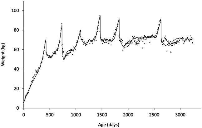
The other key element of robustness is the trade-offs between life functions. Measuring these requires a different approach as they operate over considerably longer timescales. If one is considering trade-offs between functions that are today readily measurable, such as growth and milk production, the issue is one of finding appropriate summarising measures. For a long time, a widely used summary measure of milk production was 305-day yield. However, this measure provides no information about the shape of the lactation curve making it difficult to, for example, characterise the effects of nutritional plane in early lactation on subsequent persistency. From the point of view of quantifying trade-offs between, say, milk production and body reserves, we need to describe the shapes of their profiles throughout lactation (Martin and Sauvant, Reference Martin and Sauvant2010), or at least through early lactation when the trade-off between milk production and body reserves will play on the current ability to reproduce (Ollion et al., Reference O’Mara2016). In the context of trade-offs between life stages or of predicting long-term efficiency, it is useful if these methods can be applied across life stages. As shown in Figure 9, there have been recent developments to allow this to be done. In this study (Puillet and Martin, Reference Puillet and Martin2017), a compartmental model was used to capture the coefficients describing the underlying functions of growth, body reserve gain and loss, pregnancy and lactation with respect to the BW trajectory of the animal.

Figure 9 An example of a fitting procedure using a compartmental model to decompose BW trajectories to capture (the coefficients describing) the underlying functions of growth, body reserve gain and loss, pregnancy and lactation (from birth to 8 years of age in a dairy goat). The compartmental model used is described in Puillet and Martin (Reference Puillet, Réale and Friggens2017).

In the case where the life functions that one wishes to quantify are less readily measurable in large populations, for example, immunocompetence or components of fertility, the development of precision farming technologies has great promise. There are an increasing number of biosensors being deployed on farm facilitating high-frequency measurements of key components of the functions that we wish to quantify (e.g. www.herdnavigator.com). There are also a number of technologies that will lead to the development of proxy measures. The various technologies for automated temperature measurement provide a useful health-related proxy, although at present this is almost exclusively used for monitoring rather than to phenotype this component of robustness.

As indicated above, lifetime efficiency may be the ultimate measure of robustness in farmed animals but measuring it requires measurement of feed intake. Although feed intake has long been measured in research stations, its measurement on commercial farms is greatly limited due to the high cost of the labour or equipment needed especially for grazing animals. However, promising developments in accelerometers and other technologies offer the prospect of a useful proxy measures such as time spent eating. The challenge for the future will be how to combine various proxy measures to obtain reliable estimates of intake (and other robustness- and efficiency-related elements) in large populations.

Managing robustness: genotype-by-environment interactions and selection

Genetic gain for a given trait or attribute is a function of: (1) the intensity of selection, (2) the accuracy of selection in the environment(s) of interest, (3) the extent of genetic variability in the characteristics of interest, (4) the generation interval, (5) the importance of the characteristic relative to all other animal attributes under selection and (6) the covariance that exist between the characteristic of interest and all other animal attributes in the breeding goal. A further consideration of particular relevance in the context of robustness is, to what extent the trait defined for inclusion in the breeding programme truly reflects robustness. Indeed, a paradox exists in the context of robustness where breeding programmes are now striving for homogeneity of animals while, in fact, preserving variability could be key to ensure (some) individuals are robust to the ever-changing environmental challenges. An added complication for breeding strategies is the (sometimes) relatively long time horizon until noticeable changes are observable – this implies that breeders, when constructing breeding goals for robustness, must be aware of not only the likely future production systems but also the future environmental challenges (e.g. the impact of climate change on exposure to exotic diseases).

It is clear from the preceding sections that robustness (and efficiency) is a long-term characteristic that takes cognisance of individual animal performance and functioning throughout all life stages. This therefore should ideally be captured in breeding goals. However, this is challenging for a number of reasons which are elaborated below (see also Rauw and Gomez-Raya, Reference Rauw and Gomez-Raya2015). A first issue is that when using long-term measures several permutations and combinations of phenotypes can give rise to identical final outcomes – for example, two animals can have the same productive lifespan but one received considerable more medicinal interventions throughout its lifetime and was therefore less robust; such information must be captured. The monitoring tools already exist, or are in development, to ensure that procurement of real-time accurate phenotypes for many traits does not hinder achieving accurate genetic evaluations in conventional production systems, thereby facilitating the identification of genetically diverse animals. More difficult, however, is the achievement of accurate genetic evaluations under environmental conditions less frequent in a country, particularly those that are a challenge for using monitoring technologies (e.g. organic, grazing). One strategy to overcome this is to define a series of explicit environments and exploit the correlation structure that exists among them to predict genetic merit in each environment based on estimated genetic merit in the other environments. However, the accuracy achievable is limited by the square root of the proportion of genetic variance in a given environment explained by the performance records originating from all other environments. As genetic gain is the product of several factors (Rendel and Robertson, Reference Rendel and Robertson1950), low accuracy of selection compromises genetic gain. Moreover, such a strategy only facilitates genetic evaluations in discrete environments while, in reality, there is usually a continuum of environments. Fitting random regression models across a gradient of an environmental condition (e.g. average diet density, pathogen load) enables the estimation of genetic merit of an individual across all environments (Berry et al., Reference Berry, Buckley, Dillon, Evans, Rath and Veerkamp2003); the level and slope of the individual animal deviation from the population mean regression slope can be viewed as a reaction norm. The (co)variance function can be used to estimate the extent of G×E interactions across the gradient, whereas the individual animal coefficients reflect the extent to which each individual reacts differently to changes in the prevailing environment.

The intercept and slope(s) parameters from reaction norms can be used to categorise animals into generalists or specialists. The differentiation between a generalist and specialist refers to the slope of the individual random regression; a generalist is one whose phenotype (e.g. fitness) is relatively constant irrespective of the environmental conditions it is exposed to, whereas the specialist is the opposite. A generalist may therefore be thought to be robust to environmental challenges if the dependent variable is fitness, then a generalist will retain a similar level of fitness irrespective of environment. The use of reaction norms is therefore one phenotyping strategy for characterising the robustness of individuals (Rauw and Gomez-Raya, Reference Rauw and Gomez-Raya2015), and the impact of breeding for different animal robustness types on other performance traits (e.g. lactation yield) can easily be quantified by correlating the slope of the reaction norm with the performance traits. Nonetheless it is not always possible to evaluate the performance of individuals in extreme environments (e.g. very high pathogen load which can result in considerable mortality if not genetically robust), this is especially true for the evaluation of selection candidates themselves. The advent of low-cost genomic tools, and strategies to generate accurate genetic evaluations based on genome sharing between relatives, opens the opportunity to ‘sacrifice’ close siblings of selection candidates by exposing them to harsh environments and utilising their genomic relationships with the selection candidate to obtain an accurate genetic evaluation pertinent to that environment. Up until now, without including genomic data into genetic evaluations, the maximum accuracy of selection for a candidate animal that could be achieved when phenotypes existed on full-sibs or half-sibs was 0.707 and 0.50, respectively.

The multi-component nature of robustness implies that breeding programmes must simultaneously consider all its important components. Moreover, the long time horizon to observe the true lifespan phenotype of an individual implies a reduction in annual genetic gain due to the lengthening of the generation interval in the selection. Although incorporation of genomic data into genetic evaluations can compensate for this by providing some estimate of genetic merit for lifespan, these estimates are limited in predictive ability. Moreover, lifespan in particular, is likely to suffer from G×E interactions given the likely differences in the relative importance of different traits contributing to lifespan in different environments. As previously described, the importance to lifespan of being able to cope with food shortage in wild rabbits is likely to be greater than in farmed rabbits. This, therefore, can impact the correlation structure among traits and between resilience and putative predictor traits. All of this indicates that considerable care should be taken in choosing the traits, and the timing of their measurement (stage of life, duration of measuring period), when designing breeding programmes for robustness. In addition to making best use of the biological understanding of robustness, statistical modelling issues need to also be considered. For example, a correlation measures the strength of the linear relationship among variables. If the relationship is non-linear, the estimated correlation will be a function of the mean of both traits; mean performance can differ between environments (e.g. constrained feeding v. ad libitum feeding), which has subsequent repercussions on the estimated correlations and the complexity of the breeding scheme that needs to be adopted.

Achieving high accuracy of selection without necessarily prolonging the generation interval requires the incorporation of early predictor traits into a multi-trait selection index to facilitate selection on all traits simultaneously. As stated earlier, single time-point measurements may be of limited value to quantify robustness but instead measurements over time are needed. The random regression methodology previously described for the derivation of reaction norms can also be used to model within-animal profiles over a time trajectory. The first derivative of such profiles can be used as a measure of rate of change in the trait. Such models, commonly termed test-day models, have been fitted to longitudinal data for many performance traits including milk production, body condition score and growth rate (Berry et al., Reference Berry, Buckley, Dillon, Evans, Rath and Veerkamp2003; Banos et al., Reference Banos, Brotherstone and Coffey2005). They offer a means to concisely describe key elements of robustness. For a given individual, the rates of change in one trait relative to another describe the shift in priority over time between the two traits, and thus the trade-off between them.

Genetic evaluations are based on the estimation of genetic merit of individuals while simultaneously removing the contribution of systematic environmental effects (e.g. herd) to the phenotype. The model solutions for the systematic environmental effects such as herd can, however, provide useful information of the performance of that herd for the trait under investigation relative to the population as a whole or a sample population of contemporaries. Such information can be used in two ways. It can be used to provide a quantification of the environment using the ultimate bio-monitoring system, that is, the animal (Mathur et al., Reference Mathur, Herrero-Medrano, Alexandri, Knol, ten Napel, Rashidi and Mulder2014), and has been also applied within a reaction norm approach (Knap and Su, Reference Knap and Su2008). This herd-level information also provides valuable management input. It can be used to target herd owners performing below par, to understand why, and where possible, to rectify management strategies to improve their animal robustness more in line with expectations based on genetic merit.

The use of genetic information in on-farm management can also be taken a step further. Achieving gains at farm level is not only a function of selecting the genetically elite females as potential dams of the next generation but also requires culling of females expected to generate less profit for the remainder of their lifetime. In this context, future expected resilience is a large contributor to the expected profit to be generated by a female for the remainder of her lifetime and is largely influenced by the number of remaining lactations. If the farmer, or their advisor, had this information available it would allow this factor to be used in making culling and re-breeding decisions. Kelleher et al (Reference Kelleher, Amer, Shalloo, Evans, Byrne, Buckley and Berry2015) developed what they called a culling index which considered additive genetic, non-additive genetic and animal permanent environmental effects as well as phenotypic factors of the animal itself such as age, calving date and pregnancy status. Transition matrices were used to model the likelihood of an animal surviving to the next and subsequent lactations based on her age, total genetic merit and calving date. Kelleher et al (Reference Kelleher, Amer, Shalloo, Evans, Byrne, Buckley and Berry2015) demonstrated, using validation, the superiority of using this tool to cull animals over and above culling purely on genetic merit.

Concluding remarks

Robustness and adaptive capacity are complex characteristics unlikely to be pinned down by simple combinations of raw measures but instead requiring a systemic view. Defining the level, and thus the system, to which we wish to apply the notion of robustness allows the identification of promising traits among the possible measures of phenotype. This fits very much with the approach whereby phenotyping has been driven by genetic, and then genomic, selection needs: In order to select, we need to associate the genetic architecture with phenotypic performance, and the finer the description of the genetic architecture, the finer the description of the phenotype we would like. However, there is a real sense of a need to reverse this approach to define new phenotypes that are seen as desirable because they respond to societal needs for more durable, efficient and high welfare animals; and then see how to select for them. In other words, we need to define phenotypes from consideration of their biological properties and not just from available measures.