

1 Introduction
Debris and pyroclastic flow deposits often show evidence of bouldery fronts that have a high proportion of large particles (e.g. Sharp & Nobles Reference Sharp and Nobles1953; Johnson Reference Johnson1970, Reference Johnson1984; Takahashi Reference Takahashi1980; Costa & Williams Reference Costa and Williams1984; Pierson Reference Pierson and Abrahams1986; Iverson Reference Iverson2014; Turnbull, Bowman & McElwaine Reference Turnbull, Bowman and McElwaine2015). Figure 1 shows large boulders deposited at the front of a debris flow in Arizona, USA. These large grains tend to be more resistive to downslope motion than the fines, and consequentially have a significant influence on the overall flow dynamics by acting as a ‘dam’ that resists the flow behind (Pierson Reference Pierson and Abrahams1986). The advancing, more mobile, fine grains from within the interior of the flow (Major & Iverson Reference Major and Iverson1999) shoulder the large particles at the front to the sides (Johnson et al. Reference Johnson, Kokelaar, Iverson, Logan, LaHusen and Gray2012), forming coarse-grained levees that channelise the flow. The inside of this channel is lined by a layer of deposited fine grains, further reducing the friction and increasing the run-out distance (Kokelaar et al. Reference Kokelaar, Graham, Gray and Vallance2014). All of this behaviour is readily reproduced in both large- and small-scale experiments (Iverson & Vallance Reference Iverson and Vallance2001; Iverson et al. Reference Iverson, Logan, LaHusen and Berti2010; Johnson et al. Reference Johnson, Kokelaar, Iverson, Logan, LaHusen and Gray2012). In particular, Pouliquen, Delour & Savage (Reference Pouliquen, Delour and Savage1997) observed that the interaction of the resistive front with the mobile interior also causes a lateral instability where the flow-front fingers and breaks into a number of different confining channels (Sharp & Nobles Reference Sharp and Nobles1953; Pouliquen et al. Reference Pouliquen, Delour and Savage1997; Woodhouse et al. Reference Woodhouse, Thornton, Johnson, Kokelaar and Gray2012). The development of the bouldery fronts is thus key to understanding how segregation feeds back on the bulk flow field.
Photograph of the front of a debris flow that has stopped in the channel of Rattlesnake Creek, Arizona, USA. The large boulders seen here in the front are typical of many debris and pyroclastic flows, with larger particles segregating upwards to the faster moving surface layers and preferentially transported towards the front, where they accumulate. Photo courtesy of C. Magirl and USGS.

A key component within the formation of coarse-grained fronts and lateral levees is the inherent process of size segregation that is common to all polydisperse granular media. Whilst flowing, granular mixtures dilate sufficiently to allow the flow to act like a sieve that naturally sorts the different sized constituents. Small gaps in the grain matrix allow the finer grains to preferentially percolate downwards under gravity, whilst there is a return flow of coarse grains towards the surface. The exact mechanism for the rising of large grains is under investigation (van der Vaart et al. Reference van der Vaart, Gajjar, Epely-Chauvin, Andreini, Gray and Ancey2015), although the net result is an upward coarsening in the particle-size distribution that is often called inverse grading. For example, a bidisperse mixture containing just two grain sizes would separate into two separate layers in the absence of diffusion, with the large particles on top of the small ones, as shown in figure 2(a). The surface layers have the highest velocities, and so the larger particles are transported to the front of the flow. These coarse grains may then be pushed en masse at the front if massive enough (Pouliquen & Vallance Reference Pouliquen and Vallance1999), or otherwise may be overrun by the advancing flow. They are able to rise up back towards the surface as they are resegregated, creating a complex recirculating motion that connects the upstream inversely graded body of the flow to the coarse-rich flow front. As more large grains are supplied towards the front, the coarse-grained margin grows in size, with the interface propagating forward at a slower speed than the advancing front (Gray & Kokelaar Reference Gray and Kokelaar2010a ,Reference Gray and Kokelaar b ). The front may obtain a steady size in two dimensions if there is no further upstream supply of large particles, or alternatively, if the upstream supply of large particles is matched by the rate of deposition on the lower basal surface (Gray & Ancey Reference Gray and Ancey2009). The front may also obtain a finite-size steady state in three dimensions by shouldering the large grains, transported to the front, laterally outwards to the sides to produce static coarse-grained levees (Johnson et al. Reference Johnson, Kokelaar, Iverson, Logan, LaHusen and Gray2012; Kokelaar et al. Reference Kokelaar, Graham, Gray and Vallance2014).
(a) A vertical section through a steadily propagating avalanche travelling down an inclined plane. In the body of the flow, the large grains segregate to the upper layers, where the velocity $u(z)$
is greatest, and hence are transported towards the front of the avalanche, where they are overrun, resegregated upwards and recirculated to form a coarse-rich particle front. A complex recirculating motion is created that links the vertically segregated flow in the rear of the avalanche from the coarse-grained front, with the recirculating region known as a ‘breaking size-segregation wave’ (Thornton & Gray Reference Thornton and Gray2008). Although the front increases in size as more large particles are supplied from the inversely graded flow upstream, the recirculation region shown with dotted lines reaches a steady structure that travels at the average speed
$u(z)$
is greatest, and hence are transported towards the front of the avalanche, where they are overrun, resegregated upwards and recirculated to form a coarse-rich particle front. A complex recirculating motion is created that links the vertically segregated flow in the rear of the avalanche from the coarse-grained front, with the recirculating region known as a ‘breaking size-segregation wave’ (Thornton & Gray Reference Thornton and Gray2008). Although the front increases in size as more large particles are supplied from the inversely graded flow upstream, the recirculation region shown with dotted lines reaches a steady structure that travels at the average speed $u_{wave}$
. (b) A convenient way of studying this steady recirculation regime is to use a moving-bed flume, which can establish a steady motion within a short chute length. The belt moves upstream at a speed
$u_{wave}$
. (b) A convenient way of studying this steady recirculation regime is to use a moving-bed flume, which can establish a steady motion within a short chute length. The belt moves upstream at a speed $u_{belt}$
, driving an upstream flow in the lowest layers, whilst the upper layers move downstream under gravity. This generates a net velocity profile
$u_{belt}$
, driving an upstream flow in the lowest layers, whilst the upper layers move downstream under gravity. This generates a net velocity profile $\hat{u} (z)=u(z)-u_{wave}$
and is the same as examining the recirculation zone within (a) from a frame advecting at speed
$\hat{u} (z)=u(z)-u_{wave}$
and is the same as examining the recirculation zone within (a) from a frame advecting at speed $u_{wave}$
. There is no upstream supply of large particles in this configuration (b), and so, provided that the segregation and diffusion rates are constant (Thornton & Gray Reference Thornton and Gray2008), it is mathematically equivalent to the subset of figure (a) marked by the dotted lines. Large particles rise towards the surface, and are sheared towards the downstream end of the flume. Some large grains are driven back upstream by the belt, segregate back towards the surface and are recirculated.
$u_{wave}$
. There is no upstream supply of large particles in this configuration (b), and so, provided that the segregation and diffusion rates are constant (Thornton & Gray Reference Thornton and Gray2008), it is mathematically equivalent to the subset of figure (a) marked by the dotted lines. Large particles rise towards the surface, and are sheared towards the downstream end of the flume. Some large grains are driven back upstream by the belt, segregate back towards the surface and are recirculated.

A schematic diagram of the moving-bed flume set-up. The flume is 104 cm in length and 15 cm high, with a rough 10 cm wide conveyor belt at the base that moves upstream at velocity $u_{belt}=72~\text{mm}~\text{s}^{-1}$
. This generates the flow configuration sketched in figure 2(b), with the particles in the lower layers of the flow forced upstream by the belt, whilst those in the upper layers of the flow move downstream under gravity. The entire set-up is submerged in a larger tank containing a mixture of benzyl-alcohol and ethanol. This acted as the index matched interstitial fluid, and had a viscosity
$u_{belt}=72~\text{mm}~\text{s}^{-1}$
. This generates the flow configuration sketched in figure 2(b), with the particles in the lower layers of the flow forced upstream by the belt, whilst those in the upper layers of the flow move downstream under gravity. The entire set-up is submerged in a larger tank containing a mixture of benzyl-alcohol and ethanol. This acted as the index matched interstitial fluid, and had a viscosity ${\it\mu}=3~\text{mPa}~\text{s}$
and fluid density of
${\it\mu}=3~\text{mPa}~\text{s}$
and fluid density of $995~\text{kg}~\text{m}^{-3}$
. The motor unit was mounted outside of the tank and drove the belt through a chain mechanism. A dye (rhodamine) was added to the fluid and the flow illuminated with a laser sheet of wavelength 532 nm. A camera positioned at one of the glass side walls captured the temporal evolution, with particles appearing as dark circles. The diameters of these circles could be tracked in time to determine whether the particle was small or large. An example snapshot at one moment in time, and the time-averaged concentration fields are shown in figure 6.
$995~\text{kg}~\text{m}^{-3}$
. The motor unit was mounted outside of the tank and drove the belt through a chain mechanism. A dye (rhodamine) was added to the fluid and the flow illuminated with a laser sheet of wavelength 532 nm. A camera positioned at one of the glass side walls captured the temporal evolution, with particles appearing as dark circles. The diameters of these circles could be tracked in time to determine whether the particle was small or large. An example snapshot at one moment in time, and the time-averaged concentration fields are shown in figure 6.

Photographs showing the steady recirculation regime established within the 104 cm long moving-bed flume set-up sketched in figure 3. The particle diameters were 5 and 14 mm. The normal exposure photograph (a) shows the large blue and white marbles collecting towards the right, forming a coarse-rich flow region at the downstream end of the flume, whilst the long exposure photograph (b) shows a time-averaged concentration field and the structure of the breaking size-segregation wave. An exposure time of 133 s was used to capture (b).

1.1 Recirculating particle motion
The first real insights into the structure of the recirculation zone were provided by Pouliquen et al. (Reference Pouliquen, Delour and Savage1997) and Pouliquen & Vallance (Reference Pouliquen and Vallance1999), who used a moving camera to approximately measure the lateral recirculating motion of a line of large black crushed fruit stones placed on the surface of a flow of translucent glass beads. Their observations, however, lacked spatial resolution, and further direct experimental observation of the recirculation has been challenging due to its complex time dependence. The recirculation zone propagates quickly downstream at speed $u_{wave}$
as the front advances forward at speed
$u_{wave}$
as the front advances forward at speed $u_{front}$
, meaning that there is the difficulty of capturing the motion using a camera moving with the recirculation zone. Long chutes are also required before a steady recirculation regime emerges.
$u_{front}$
, meaning that there is the difficulty of capturing the motion using a camera moving with the recirculation zone. Long chutes are also required before a steady recirculation regime emerges.
An alternative approach is to use the moving-bed flume set-up shown in figure 3, that is similar to that used by Davies (Reference Davies1990). The flume is 104 cm in length with a rough 10 cm wide upward moving conveyor belt positioned between the four stationary vertical walls. The inclination of the channel was set at 19.8° to establish a uniform flow height along the channel. Higher or lower angles were found to cause an accumulation towards the front or rear of the channel, respectively. The belt moves upstream at a velocity $u_{belt}=72~\text{mm}~\text{s}^{-1}$
. This generates the experimental configuration shown schematically in figure 2(b), where the lower layers of the flow are forced upstream by the belt, while the upper layers move downstream under gravity. While this flow is not itself inversely graded, it is mathematically equivalent to the section of an inversely graded avalanche shown in figure 2(a), provided that the segregation and diffusion rates are constant (Thornton & Gray Reference Thornton and Gray2008). The absence of the layer of large particles also allows a steady state to develop within the experimental configuration. Both the experimental configuration and the full problem are assumed to be two-dimensional, meaning that there are no side-wall effects. Just as in the full problem, the large grains in the experimental configuration (figure 2
b) initially segregate upwards and are sheared towards the downstream end of the flume, as shown in the normal exposure photograph in figure 4(a). However, the motion of the belt forces some large grains to be carried upstream, where they subsequently lie below small grains. The large grains resegregate upwards, and once they reach the surface, they are carried back towards the downstream end of the flume. The oblique view in figure 5 looking upstream from the end of the flume clearly shows the accumulated large particles, and resembles the bouldery front shown in figure 1. This moving-bed flume allows the structure of the steady recirculation regime to be examined in greater detail. For example, the long time exposure photograph in 4(b), taken with an exposure time of 133 s, illustrates the time-averaged concentration field of the recirculation zone.
$u_{belt}=72~\text{mm}~\text{s}^{-1}$
. This generates the experimental configuration shown schematically in figure 2(b), where the lower layers of the flow are forced upstream by the belt, while the upper layers move downstream under gravity. While this flow is not itself inversely graded, it is mathematically equivalent to the section of an inversely graded avalanche shown in figure 2(a), provided that the segregation and diffusion rates are constant (Thornton & Gray Reference Thornton and Gray2008). The absence of the layer of large particles also allows a steady state to develop within the experimental configuration. Both the experimental configuration and the full problem are assumed to be two-dimensional, meaning that there are no side-wall effects. Just as in the full problem, the large grains in the experimental configuration (figure 2
b) initially segregate upwards and are sheared towards the downstream end of the flume, as shown in the normal exposure photograph in figure 4(a). However, the motion of the belt forces some large grains to be carried upstream, where they subsequently lie below small grains. The large grains resegregate upwards, and once they reach the surface, they are carried back towards the downstream end of the flume. The oblique view in figure 5 looking upstream from the end of the flume clearly shows the accumulated large particles, and resembles the bouldery front shown in figure 1. This moving-bed flume allows the structure of the steady recirculation regime to be examined in greater detail. For example, the long time exposure photograph in 4(b), taken with an exposure time of 133 s, illustrates the time-averaged concentration field of the recirculation zone.
An oblique upstream view from the surface of steady-state coarse-rich front established in the moving-bed flume of figure 3. The large blue and white marbles congregate towards the front of the picture, with the smaller clear glass beads towards the rear.

The individual motion of the particles on the centre line was revealed using refractive index matched scanning (‘RIMS’: Wiederseiner et al.
Reference Wiederseiner, Andreini, Epely-Chauvin and Ancey2011a
; Dijksman et al.
Reference Dijksman, Rietz, Lorincz, van Hecke and Losert2012; van der Vaart et al.
Reference van der Vaart, Gajjar, Epely-Chauvin, Andreini, Gray and Ancey2015). Spherical borosilicate glass beads of density $2230~\text{kg}~\text{m}^{-3}$
and diameters 14 and 5 mm were used, with the volume ratio of large particles to small particles being 2 : 5. As shown in figure 3, the entire flume set-up was submerged in a tank containing a mixture of benzyl-alcohol and ethanol, which acted as the index matched interstitial fluid of viscosity
$2230~\text{kg}~\text{m}^{-3}$
and diameters 14 and 5 mm were used, with the volume ratio of large particles to small particles being 2 : 5. As shown in figure 3, the entire flume set-up was submerged in a tank containing a mixture of benzyl-alcohol and ethanol, which acted as the index matched interstitial fluid of viscosity ${\it\mu}=3~\text{mPa}~\text{s}$
, with a fluid density of
${\it\mu}=3~\text{mPa}~\text{s}$
, with a fluid density of $995~\text{kg}~\text{m}^{-3}$
. The motor unit for the belt was positioned outside of the tank and drove the belt through a system of chains. A fluorescent dye (rhodamine) was added to the liquid, which was excited by a laser sheet of wavelength 532 nm in a thin plane parallel to the flow direction. As the particles contain no dye, they appear as dark circles on a bright background. The result is a cross-sectional image of the interior of the flow, which is captured through the glass side wall using a high-speed camera. The laser and camera were positioned to capture the section of the flow containing the recirculation zone. The dark circles are tracked over time, with the minimum and maximum diameters used to determine whether that circle corresponds to a small or large particle. The large size ratio between the grains minimised identification errors, although there was a small possibility that a large particle may be mistaken for a small particle. This, however, would only happen if the particle was sliced close to its edge and never moved closer to the plane of the laser. A typical snapshot of the particle motion is shown in figure 6(a), where it can be seen that there are a few large particles in regions of many small particles at the upstream (left) end of the flow. These large particles are seen to move very slowly, compared with the majority of the large particles which recirculate very quickly towards the front. Figure 6(c) shows a time-averaged concentration plot, which was averaged over a 40 min period, with 1 image taken every 2 s. The slow movement of the large particles through the upstream region of small particles lowers the concentration there, and causes the ‘white’ ‘tail’-like region.
$995~\text{kg}~\text{m}^{-3}$
. The motor unit for the belt was positioned outside of the tank and drove the belt through a system of chains. A fluorescent dye (rhodamine) was added to the liquid, which was excited by a laser sheet of wavelength 532 nm in a thin plane parallel to the flow direction. As the particles contain no dye, they appear as dark circles on a bright background. The result is a cross-sectional image of the interior of the flow, which is captured through the glass side wall using a high-speed camera. The laser and camera were positioned to capture the section of the flow containing the recirculation zone. The dark circles are tracked over time, with the minimum and maximum diameters used to determine whether that circle corresponds to a small or large particle. The large size ratio between the grains minimised identification errors, although there was a small possibility that a large particle may be mistaken for a small particle. This, however, would only happen if the particle was sliced close to its edge and never moved closer to the plane of the laser. A typical snapshot of the particle motion is shown in figure 6(a), where it can be seen that there are a few large particles in regions of many small particles at the upstream (left) end of the flow. These large particles are seen to move very slowly, compared with the majority of the large particles which recirculate very quickly towards the front. Figure 6(c) shows a time-averaged concentration plot, which was averaged over a 40 min period, with 1 image taken every 2 s. The slow movement of the large particles through the upstream region of small particles lowers the concentration there, and causes the ‘white’ ‘tail’-like region.
(a) An experimental snapshot of the recirculation zone, captured using the moving-bed flume of figure 3 with refractive index matched scanning. The white label indicates the length scale of 14 mm. (b) Structure of the recirculation zone found using DPM simulations. The fixed base particles are shown in grey. Both the experimental and simulation results show several large particles positioned towards the rear, where they are surrounded by many small particles. These large particles are seen to move very slowly, and take a long time to recirculate. (c) Shows the experimental time-averaged concentration field, which was produced by averaging the individual particle positions over a 40 min period, with 1 image every 2 s. The time-averaged concentration field for the simulations was produced by coarse graining all of the particle positions from 749 subsequent time frames, and is shown in (d). Both of the time-averaged concentration plots indicate a ‘tail’ upstream, where the concentration is lower due to the slow motion of a few large grains. This is similar to asymmetric behaviour observed within a linear shear cell (van der Vaart et al. Reference van der Vaart, Gajjar, Epely-Chauvin, Andreini, Gray and Ancey2015), and motivates a continuum breaking wave structure with an asymmetric flux function, shown in (e) for a cubic flux. The solid lines mark the boundaries of the recirculation zone, with two distinct ‘lens’ and ‘tail’ regions (see § 2). The downstream ‘lens’ region with a strong green hue is where most of the large particles recirculate, whilst the red hue of the upstream ‘tail’ region shows how only a few large particles recirculate through that area. The theory does not account for spatial velocity variations, diffusive remixing or differential particle friction, and finite-size effects are also significant. These may all contribute to the difference in the ‘tail’ structure between the theory and the experiments and simulations. Without calibrating the segregation flux for this particular flow regime, it is remarkable that the asymmetric flux produces a ‘tail’ region, and it is of interest to further understand the asymmetric breaking-wave structure and particle recirculation within it. In all of the above plots, the lower belt moves from right to left, with gravity acting to cause particles to flow downstream towards the right.

It is worthwhile considering what influence the interstitial fluid has on the particle behaviour. The presence of a fluid (rather than air) not only modifies the interstitial pore pressures, but also couples the stress carried by the particles to that carried by the fluid flowing through gaps in the grain matrix (Iverson & LaHusen Reference Iverson and LaHusen1989; Iverson Reference Iverson1997, Reference Iverson2005). This coupling is particularly significant in unsteady flows, since local changes in the particle volume fraction allow large excess pore pressures to develop, which in turn feedback on the granular motion (du Pont et al. Reference du Pont, Gondret, Perrin and Rabaud2003; Muite, Hunt & Joseph Reference Muite, Hunt and Joseph2004; Pailha, Nicolas & Pouliquen Reference Pailha, Nicolas and Pouliquen2008; Pailha & Pouliquen Reference Pailha and Pouliquen2009). However, for steady, dense granular flows such as those sketched in figure 2, the large number of particle–particle contacts mean that frictional interactions are still dominant in determining the rheological behaviour (Ancey, Coussot & Evesque Reference Ancey, Coussot and Evesque1999) even when an interstitial fluid is present. Cassar, Nicolas & Pouliquen (Reference Cassar, Nicolas and Pouliquen2005) showed that, in steady flows submerged in water, at least 75 % of the overburden pressure is borne by the contact network. They also showed that the same rheology used to describe dense steady aerial flows (GDR Midi Reference GDR Midi2004) also applies to immersed flows, with the interstitial fluid changing the time scale of the particle rearrangements. This is consistent with the experimental results of Vallance & Savage (Reference Vallance, Savage, Rosato and Blackmore2000) and the theory of Thornton, Gray & Hogg (Reference Thornton, Gray and Hogg2006) who both showed that the role of the interstitial fluid in flows containing different sized constituents is to modify the segregation time scales. These results would suggest that the physical phenomena observed in the experiments above, with a few large particles recirculating very slowly in regions of small particles, are indicative an underlying asymmetry in the particle motion that occurs whether the flow is dry or submerged. Further experimental work, using techniques such as X-ray tomography (e.g. McDonald, Harris & Withers Reference McDonald, Harris and Withers2012), is needed to compare the particle scale dynamics in dry flows with those containing an interstitial fluid.
Discrete particle method (DPM) simulations of a moving bed-flume set-up were also performed using the MercuryDPM code (MercuryDPM.org; Thornton et al.
Reference Thornton, Krijgsman, Fransen, Gonzalez, Tunuguntla, ten Voortwis, Luding, Bokhove and Weinhart2013a
,Reference Thornton, Krijgsman, te Voortwis, Ogarko, Luding, Fransen, Gonzalez, Bokhove, Imole and Weinhart
b
). A dry bidisperse mixture of spherical particles was used, with all of the particles of the same (non-dimensional) density ${\it\rho}^{\ast }={\rm\pi}/6$
, but of two different (non-dimensional) diameters,
${\it\rho}^{\ast }={\rm\pi}/6$
, but of two different (non-dimensional) diameters, $d^{s}=1$
and
$d^{s}=1$
and $d^{l}=2.4$
, for small and large particles, respectively. All of the simulation parameters were non-dimensionalised so that
$d^{l}=2.4$
, for small and large particles, respectively. All of the simulation parameters were non-dimensionalised so that $g=1$
. A frictional spring-dashpot model (Cundall & Strack Reference Cundall and Strack1979; Weinhart et al.
Reference Weinhart, Thornton, Luding and Bokhove2012) with linear elastic and linear dissipative contributions was used for both the normal and tangential forces. The tangential force models the effects of particle surface roughness, and its spring stiffness was taken to be
$g=1$
. A frictional spring-dashpot model (Cundall & Strack Reference Cundall and Strack1979; Weinhart et al.
Reference Weinhart, Thornton, Luding and Bokhove2012) with linear elastic and linear dissipative contributions was used for both the normal and tangential forces. The tangential force models the effects of particle surface roughness, and its spring stiffness was taken to be $2/7$
of the spring stiffness for the normal direction. The tangential force also truncates so that it is always less than
$2/7$
of the spring stiffness for the normal direction. The tangential force also truncates so that it is always less than $1/2$
of the normal force. The particles all had the same coefficient of restitution
$1/2$
of the normal force. The particles all had the same coefficient of restitution $r_{c}=0.1538$
, which was chosen to be less than typical known values for glass
$r_{c}=0.1538$
, which was chosen to be less than typical known values for glass $({\sim}\!0.9)$
in order to model the dissipative effects of the interstitial fluid removing energy from the system. The contact time for all head on collisions was fixed at 0.0054, with the collision properties chosen to be different for small/small, small/large and large/large collisions so that both the contact time and the coefficient of restitution were the same even in the mixed case. Further details of the precise DPM implementation may be found in Thornton et al. (Reference Thornton, Weinhart, Luding and Bokhove2012b
) and Weinhart et al. (Reference Weinhart, Thornton, Luding and Bokhove2012). The simulations were conducted in a box of length
$({\sim}\!0.9)$
in order to model the dissipative effects of the interstitial fluid removing energy from the system. The contact time for all head on collisions was fixed at 0.0054, with the collision properties chosen to be different for small/small, small/large and large/large collisions so that both the contact time and the coefficient of restitution were the same even in the mixed case. Further details of the precise DPM implementation may be found in Thornton et al. (Reference Thornton, Weinhart, Luding and Bokhove2012b
) and Weinhart et al. (Reference Weinhart, Thornton, Luding and Bokhove2012). The simulations were conducted in a box of length $300d^{s}$
with fixed end walls and width
$300d^{s}$
with fixed end walls and width $8.4d^{s}$
. The side walls were periodic in order to bring the simulations closer to the assumptions of the analytic model in figure 2(b), which is two-dimensional and has no side-wall effects. A small inclined wall was placed between the base and the vertical upstream wall in order to prevent small particles being crushed by the wall or shooting away from it. This was seen to only affect the dynamics very close to the wall, and did not affect the recirculation zone. A rough moving base was created in several steps. Firstly, particles of diameter
$8.4d^{s}$
. The side walls were periodic in order to bring the simulations closer to the assumptions of the analytic model in figure 2(b), which is two-dimensional and has no side-wall effects. A small inclined wall was placed between the base and the vertical upstream wall in order to prevent small particles being crushed by the wall or shooting away from it. This was seen to only affect the dynamics very close to the wall, and did not affect the recirculation zone. A rough moving base was created in several steps. Firstly, particles of diameter $d^{b}=1.7$
were stuck randomly to a horizontal plate. Particles of diameter
$d^{b}=1.7$
were stuck randomly to a horizontal plate. Particles of diameter $d^{b}$
were slowly dropped onto this plate and allowed to settle. Once a thick layer of height
$d^{b}$
were slowly dropped onto this plate and allowed to settle. Once a thick layer of height $12d^{b}$
was produced, a slice of particles was taken whose centres lay between
$12d^{b}$
was produced, a slice of particles was taken whose centres lay between $9.3d^{b}$
and
$9.3d^{b}$
and $11d^{b}$
. These particles were endowed with infinite mass and inclined at an angle of
$11d^{b}$
. These particles were endowed with infinite mass and inclined at an angle of $23^{\circ }$
to form the base for the moving-bed flume simulations. The layer is thick enough to ensure that no flowing particles can fall through the rough base during the simulations. More details of this base creation process can be found in Weinhart et al. (Reference Weinhart, Thornton, Luding and Bokhove2012) whereas a detailed description of different bed creation methods and their effect on the macroscopic friction experienced by the flow can be found in Thornton et al. (Reference Thornton, Weinhart, Luding. and Bokhove2012a
). Before each time step
$23^{\circ }$
to form the base for the moving-bed flume simulations. The layer is thick enough to ensure that no flowing particles can fall through the rough base during the simulations. More details of this base creation process can be found in Weinhart et al. (Reference Weinhart, Thornton, Luding and Bokhove2012) whereas a detailed description of different bed creation methods and their effect on the macroscopic friction experienced by the flow can be found in Thornton et al. (Reference Thornton, Weinhart, Luding. and Bokhove2012a
). Before each time step ${\rm\Delta}t=10^{-4}\sqrt{d^{s}/g}$
, the base was moved upstream by a distance
${\rm\Delta}t=10^{-4}\sqrt{d^{s}/g}$
, the base was moved upstream by a distance $u_{belt}{\rm\Delta}t=1.5\times 10^{-4}d^{s}$
. The system was allowed to evolve until a steady recirculation zone was formed.
$u_{belt}{\rm\Delta}t=1.5\times 10^{-4}d^{s}$
. The system was allowed to evolve until a steady recirculation zone was formed.
Figure 6(b) shows a snapshot from the simulations, which have a very similar structure to the experimental results: most large particles recirculate quickly at the front but a few large particles recirculate slowly at the rear. This behaviour is also evident in the time- and width-averaged concentration plot shown in figure 6(d), which was produced by employing the micro–macro coarse-graining technique (Goldhirsch Reference Goldhirsch2010; Weinhart et al.
Reference Weinhart, Hartkamp, Thornton and Luding2013) on the individual particle positions from 749 subsequent time steps. The new extension by Tunuguntla, Thornton & Weinhart (Reference Tunuguntla, Thornton and Weinhart2015), based on a mixture theory formulation (Morland Reference Morland1992), allowed the (partial) densities for the bulk ( ${\it\rho}$
), small (
${\it\rho}$
), small ( ${\it\rho}^{s}$
) and large particles (
${\it\rho}^{s}$
) and large particles ( ${\it\rho}^{l}$
) to be separately extracted, with the small particle concentration defined as
${\it\rho}^{l}$
) to be separately extracted, with the small particle concentration defined as ${\it\rho}^{s}/{\it\rho}$
, i.e. the local small particle material density over the local granular material density. The coarse-graining method used two-dimensional Gaussian functions at each of the particle positions and generated the continuum field at every point in space; however, for ease of computing, the data is shown on a
${\it\rho}^{s}/{\it\rho}$
, i.e. the local small particle material density over the local granular material density. The coarse-graining method used two-dimensional Gaussian functions at each of the particle positions and generated the continuum field at every point in space; however, for ease of computing, the data is shown on a $250\times 250$
grid. As was seen in the experimental concentration field in figure 6(c), the slow moving large particles have lowered the upstream concentration and produced a white ‘tail’ protruding backwards from the main region of recirculation. This qualitative similarity between the concentration field of the simulations that were laterally periodic (figure 6
d) and the concentration field of the experiments (figure 6
c) indicates that there are only minimal effects arising from the side walls and justifies the two-dimensional approximation of the analytic solution. Dry simulations, using a much higher restitution coefficient, also gave a similar concentration field, indicating that the behaviour is not an artefact of the presence of the fluid nor the exact particle properties. Despite the fact that no attempt was made to calibrate the simulations and experiments, both show very similar behaviour using different sized particles in different sized flumes. The presence of the ‘tail’, in which large particles recirculate very slowly through regions of many small particles, points towards a fundamental asymmetry in the interactions between the large and small particles. Recently, van der Vaart et al. (Reference van der Vaart, Gajjar, Epely-Chauvin, Andreini, Gray and Ancey2015) uncovered a similar asymmetry in a linear shear cell, and showed how the asymmetry could be modelled using a continuum approach.
$250\times 250$
grid. As was seen in the experimental concentration field in figure 6(c), the slow moving large particles have lowered the upstream concentration and produced a white ‘tail’ protruding backwards from the main region of recirculation. This qualitative similarity between the concentration field of the simulations that were laterally periodic (figure 6
d) and the concentration field of the experiments (figure 6
c) indicates that there are only minimal effects arising from the side walls and justifies the two-dimensional approximation of the analytic solution. Dry simulations, using a much higher restitution coefficient, also gave a similar concentration field, indicating that the behaviour is not an artefact of the presence of the fluid nor the exact particle properties. Despite the fact that no attempt was made to calibrate the simulations and experiments, both show very similar behaviour using different sized particles in different sized flumes. The presence of the ‘tail’, in which large particles recirculate very slowly through regions of many small particles, points towards a fundamental asymmetry in the interactions between the large and small particles. Recently, van der Vaart et al. (Reference van der Vaart, Gajjar, Epely-Chauvin, Andreini, Gray and Ancey2015) uncovered a similar asymmetry in a linear shear cell, and showed how the asymmetry could be modelled using a continuum approach.
1.2 Continuum segregation equation for bidisperse mixtures
Non-dimensional continuum models for segregation in bidisperse mixtures (e.g. Bridgwater, Foo & Stephens Reference Bridgwater, Foo and Stephens1985; Savage & Lun Reference Savage and Lun1988; Bridgwater Reference Bridgwater and Mehta1994; Dolgunin & Ukolov Reference Dolgunin and Ukolov1995; Gray & Thornton Reference Gray and Thornton2005; Gray & Chugunov Reference Gray and Chugunov2006; Thornton et al. Reference Thornton, Gray and Hogg2006; May, Shearer & Daniels Reference May, Shearer and Daniels2010) all share a similar advection–diffusion structure
 $$\begin{eqnarray}\displaystyle {\displaystyle \frac{\partial {\it\phi}}{\partial t}}+\boldsymbol{{\rm\nabla}}\boldsymbol{\cdot }({\it\phi}\boldsymbol{u})-{\displaystyle \frac{\partial }{\partial z}}(S_{r}F({\it\phi}))={\displaystyle \frac{\partial }{\partial z}}\left(D_{r}{\displaystyle \frac{\partial {\it\phi}}{\partial z}}\right), & & \displaystyle\end{eqnarray}$$
where the $z$
coordinate is the upward pointing normal to the flume bed, the
$z$
coordinate is the upward pointing normal to the flume bed, the $x$
coordinate points down the flume and the
$x$
coordinate points down the flume and the $y$
coordinate points horizontally across the flume bed. The bulk velocity field
$y$
coordinate points horizontally across the flume bed. The bulk velocity field $\boldsymbol{u}=(u,v,w)$
has components in the above directions, the small particle concentration is
$\boldsymbol{u}=(u,v,w)$
has components in the above directions, the small particle concentration is ${\it\phi}$
, and
${\it\phi}$
, and $S_{r}$
and
$S_{r}$
and $D_{r}$
are the non-dimensional segregation and diffusive-remixing coefficients, respectively. As the typical length and height of the avalanche are
$D_{r}$
are the non-dimensional segregation and diffusive-remixing coefficients, respectively. As the typical length and height of the avalanche are $L$
and
$L$
and $H$
, and magnitudes of the downstream and segregation velocities are
$H$
, and magnitudes of the downstream and segregation velocities are $U$
and
$U$
and $Q$
, the non-dimensional segregation coefficient
$Q$
, the non-dimensional segregation coefficient $S_{r}=QL/(HU)$
represents the ratio of the typical segregation time scale
$S_{r}=QL/(HU)$
represents the ratio of the typical segregation time scale $Q/H$
to the typical downstream transport time scale
$Q/H$
to the typical downstream transport time scale $U/L$
. Similarly, the non-dimensional diffusion coefficient
$U/L$
. Similarly, the non-dimensional diffusion coefficient $D_{r}=DL/(H^{2}U)$
represents the ratio of the typical diffusion time scale
$D_{r}=DL/(H^{2}U)$
represents the ratio of the typical diffusion time scale $D/H^{2}$
to the typical downstream transport time scale
$D/H^{2}$
to the typical downstream transport time scale $U/L$
, with
$U/L$
, with $D$
being the diffusivity between the two particle species. The large particle concentration is
$D$
being the diffusivity between the two particle species. The large particle concentration is $1-{\it\phi}$
since the solids volume fraction is assumed to be uniform and constant throughout the flowing layer (Rognon et al.
Reference Rognon, Roux, Naaim and Chevoir2007). The first term on the left-hand side in (1.1) describes the temporal evolution, whilst the second term describes the advection with the bulk flow. The segregation is captured by the third term, with
$1-{\it\phi}$
since the solids volume fraction is assumed to be uniform and constant throughout the flowing layer (Rognon et al.
Reference Rognon, Roux, Naaim and Chevoir2007). The first term on the left-hand side in (1.1) describes the temporal evolution, whilst the second term describes the advection with the bulk flow. The segregation is captured by the third term, with $F({\it\phi})$
the segregation flux and the negative sign indicating that there is a net motion of small particles downwards. The segregation flux is often assumed to be the product of the small and large particle concentrations,
$F({\it\phi})$
the segregation flux and the negative sign indicating that there is a net motion of small particles downwards. The segregation flux is often assumed to be the product of the small and large particle concentrations,
 $$\begin{eqnarray}\displaystyle F({\it\phi})={\it\phi}(1-{\it\phi}), & & \displaystyle\end{eqnarray}$$
and has the property that segregation ceases when the concentration reaches zero (pure large phase) or unity (pure small phase). The right-hand side of equation (1.1) reduces the sharp concentration shocks that develop between the two species, and models the diffusion of one species into the other that results from the random-walk-like behaviour of the grains. In many flows, this is small compared to the segregation (Gray & Hutter Reference Gray and Hutter1997; Dasgupta & Manna Reference Dasgupta and Manna2011; Wiederseiner et al.
Reference Wiederseiner, Andreini, Epely-Chauvin, Moser, Monnereau, Gray and Ancey2011b
; Thornton et al.
Reference Thornton, Weinhart, Luding and Bokhove2012b
) and so the non-diffuse solution in which $D_{r}=0$
is a useful approximation, with (1.1) reducing to a scalar hyperbolic equation. A full review of the derivation, history and applications of (1.1) can be found in Gray, Gajjar & Kokelaar (Reference Gray, Gajjar and Kokelaar2015).
$D_{r}=0$
is a useful approximation, with (1.1) reducing to a scalar hyperbolic equation. A full review of the derivation, history and applications of (1.1) can be found in Gray, Gajjar & Kokelaar (Reference Gray, Gajjar and Kokelaar2015).
1.3 Asymmetry between large and small particle motion
Recent experiments by Golick & Daniels (Reference Golick and Daniels2009) and van der Vaart et al. (Reference van der Vaart, Gajjar, Epely-Chauvin, Andreini, Gray and Ancey2015) have uncovered an underlying asymmetry in the behaviour of large and small grains during segregation, with a characteristic dependence on the local relative volume fraction of small particles. Within their annular ring shear experiments, Golick & Daniels (Reference Golick and Daniels2009) inferred that large particles were segregating very slowly in regions of many small particles, but were not able to further explain this observation. Using a classical linear shear cell (Bridgwater Reference Bridgwater1976) and the ‘refractive index matched scanning technique’ (Wiederseiner et al.
Reference Wiederseiner, Andreini, Epely-Chauvin and Ancey2011a
; Dijksman et al.
Reference Dijksman, Rietz, Lorincz, van Hecke and Losert2012), experiments by van der Vaart et al. quantified on both bulk and particle scales how large particles rise slower in regions of many small particles compared to small particles percolating down through a region of many large particles. They also showed that the large particle velocity displayed a peak at approximately ${\it\phi}=0.55$
, proving that the coarse grains rise quickest as a group. Gajjar & Gray (Reference Gajjar and Gray2014) showed that the normal constituent velocities associated with the segregation equation (1.1) are
${\it\phi}=0.55$
, proving that the coarse grains rise quickest as a group. Gajjar & Gray (Reference Gajjar and Gray2014) showed that the normal constituent velocities associated with the segregation equation (1.1) are
 $$\begin{eqnarray}\displaystyle w^{l}({\it\phi})=w+S_{r}{\displaystyle \frac{F({\it\phi})}{1-{\it\phi}}},\quad w^{s}({\it\phi})=w-S_{r}{\displaystyle \frac{F({\it\phi})}{{\it\phi}}}, & & \displaystyle\end{eqnarray}$$
with both velocities uniquely determined by the geometry of the flux function $F({\it\phi})$
at every concentration
$F({\it\phi})$
at every concentration ${\it\phi}$
. The velocity of the large particles
${\it\phi}$
. The velocity of the large particles $w^{l}({\it\phi})$
(1.3a
) is directly proportional to the gradient of the chord, namely the gradient of the straight line segment (Clapham & Nicholson Reference Clapham and Nicholson2009), joining
$w^{l}({\it\phi})$
(1.3a
) is directly proportional to the gradient of the chord, namely the gradient of the straight line segment (Clapham & Nicholson Reference Clapham and Nicholson2009), joining $(1,0)$
with
$(1,0)$
with $({\it\phi},F({\it\phi}))$
. Similarly, the velocity of the small particles
$({\it\phi},F({\it\phi}))$
. Similarly, the velocity of the small particles $w^{s}({\it\phi})$
is directly proportional to the gradient of the chord joining
$w^{s}({\it\phi})$
is directly proportional to the gradient of the chord joining $(0,0)$
with
$(0,0)$
with $({\it\phi},F({\it\phi}))$
. A pair of these two chords for
$({\it\phi},F({\it\phi}))$
. A pair of these two chords for ${\it\phi}={\it\phi}_{max}$
are shown in figure 7(b). Since the quadratic segregation flux (1.2) utilised by many segregation models is symmetric about
${\it\phi}={\it\phi}_{max}$
are shown in figure 7(b). Since the quadratic segregation flux (1.2) utilised by many segregation models is symmetric about ${\it\phi}=0.5$
(figure 7
a), it gives linear segregation velocities for the large and small grains
${\it\phi}=0.5$
(figure 7
a), it gives linear segregation velocities for the large and small grains
 $$\begin{eqnarray}\displaystyle w^{l}({\it\phi})=w+S_{r}{\it\phi},\quad w^{s}({\it\phi})=w-S_{r}(1-{\it\phi}). & & \displaystyle\end{eqnarray}$$
The maxima of these velocities are equal in magnitude (figure 7
c), and so (1.2) is unable to capture the asymmetry measured by van der Vaart et al. (Reference van der Vaart, Gajjar, Epely-Chauvin, Andreini, Gray and Ancey2015). In order to model the asymmetric behaviour between large and small grains, Gajjar & Gray (Reference Gajjar and Gray2014) introduced a new class of flux functions with the following properties: (i) $F({\it\phi})$
is skewed towards
$F({\it\phi})$
is skewed towards ${\it\phi}=0$
, with a maximum occurring at
${\it\phi}=0$
, with a maximum occurring at $0<{\it\phi}_{max}<1/2$
; (ii)
$0<{\it\phi}_{max}<1/2$
; (ii) $F({\it\phi})$
is normalised to have the same amplitude as the quadratic flux (1.2); and (iii)
$F({\it\phi})$
is normalised to have the same amplitude as the quadratic flux (1.2); and (iii) $F({\it\phi})$
has at most one inflexion point
$F({\it\phi})$
has at most one inflexion point ${\it\phi}_{inf}$
in the interval
${\it\phi}_{inf}$
in the interval $({\it\phi}_{max},1)$
. Although there are other ways of normalising the class of flux functions, e.g. by the area, there were no qualitative differences between the different methods. The simplest flux function fitting all of the above requirements is the cubic form
$({\it\phi}_{max},1)$
. Although there are other ways of normalising the class of flux functions, e.g. by the area, there were no qualitative differences between the different methods. The simplest flux function fitting all of the above requirements is the cubic form
 $$\begin{eqnarray}\displaystyle F({\it\phi})=A_{{\it\gamma}}{\it\phi}(1-{\it\phi})(1-{\it\gamma}{\it\phi}), & & \displaystyle\end{eqnarray}$$
where ${\it\gamma}$
is the asymmetry parameter and
${\it\gamma}$
is the asymmetry parameter and $A_{{\it\gamma}}$
is a normalisation constant. Note that the limit
$A_{{\it\gamma}}$
is a normalisation constant. Note that the limit ${\it\gamma}\rightarrow 0$
of (1.5) recovers the symmetric quadratic flux (1.2). For small amounts of asymmetry,
${\it\gamma}\rightarrow 0$
of (1.5) recovers the symmetric quadratic flux (1.2). For small amounts of asymmetry, $0\leqslant {\it\gamma}\leqslant 0.5$
,
$0\leqslant {\it\gamma}\leqslant 0.5$
, $F({\it\phi})$
is convex up (Clapham & Nicholson Reference Clapham and Nicholson2009), whilst for greater amounts of asymmetry
$F({\it\phi})$
is convex up (Clapham & Nicholson Reference Clapham and Nicholson2009), whilst for greater amounts of asymmetry $0.5<{\it\gamma}\leqslant 1$
,
$0.5<{\it\gamma}\leqslant 1$
, $F({\it\phi})$
is non-convex with a single inflexion point
$F({\it\phi})$
is non-convex with a single inflexion point
 $$\begin{eqnarray}\displaystyle {\it\phi}_{inf}={\displaystyle \frac{1+{\it\gamma}}{3{\it\gamma}}}. & & \displaystyle\end{eqnarray}$$
As shown in figure 7(c), the cubic functions (1.5) are able to reproduce the asymmetric behaviour that a small particle will percolate down more quickly at low ${\it\phi}$
(figure 7
e) than a large particle rises upwards at high
${\it\phi}$
(figure 7
e) than a large particle rises upwards at high ${\it\phi}$
(figure 7
g). In addition, figure 7(b) shows how the presence of an inflexion point (1.6) means that the chord joining
${\it\phi}$
(figure 7
g). In addition, figure 7(b) shows how the presence of an inflexion point (1.6) means that the chord joining $({\it\phi},F({\it\phi}))$
with
$({\it\phi},F({\it\phi}))$
with $(1,0)$
initially has an increasing gradient as
$(1,0)$
initially has an increasing gradient as ${\it\phi}$
increases from 0 to
${\it\phi}$
increases from 0 to ${\it\phi}_{\text{M}}$
, and a decreasing gradient thereafter. Thus, the non-convex flux functions display a maximum in the large particle velocity at an intermediate concentration
${\it\phi}_{\text{M}}$
, and a decreasing gradient thereafter. Thus, the non-convex flux functions display a maximum in the large particle velocity at an intermediate concentration ${\it\phi}_{\text{M}}$
(figure 7
f). This behaviour will be known as the collective motion of the large particles.
${\it\phi}_{\text{M}}$
(figure 7
f). This behaviour will be known as the collective motion of the large particles.
There is an intrinsic geometric relationship between the segregation flux $F({\it\phi})$
shown in (a), and its segregation velocities
$F({\it\phi})$
shown in (a), and its segregation velocities $w^{{\it\nu}}$
(1.3) shown in (c). At any concentration
$w^{{\it\nu}}$
(1.3) shown in (c). At any concentration ${\it\phi}$
, the gradient of the chords (straight line segment) joining
${\it\phi}$
, the gradient of the chords (straight line segment) joining $({\it\phi},F({\it\phi}))$
with
$({\it\phi},F({\it\phi}))$
with $(1,0)$
and
$(1,0)$
and $(0,0)$
are proportional to the velocities (1.3) of the large and small particles, respectively. These chords are illustrated in (b) for
$(0,0)$
are proportional to the velocities (1.3) of the large and small particles, respectively. These chords are illustrated in (b) for ${\it\phi}={\it\phi}_{max}={\it\phi}_{\text{R}}$
. The quadratic flux (1.2) is symmetric about
${\it\phi}={\it\phi}_{max}={\it\phi}_{\text{R}}$
. The quadratic flux (1.2) is symmetric about ${\it\phi}=0.5$
, and thus gives linear segregation velocities (1.4) that have the same magnitude. The cubic flux is skewed towards
${\it\phi}=0.5$
, and thus gives linear segregation velocities (1.4) that have the same magnitude. The cubic flux is skewed towards ${\it\phi}=0$
with a maximum occurring at
${\it\phi}=0$
with a maximum occurring at $0<{\it\phi}_{max}={\it\phi}_{\text{R}}<1/2$
, and is normalised by (2.8) to have the same amplitude as the quadratic flux. This gives asymmetric segregation velocities, with a single small particle (e) having a greater velocity that a single large particle (g). For higher amounts of asymmetry, measured by the asymmetry parameter
$0<{\it\phi}_{max}={\it\phi}_{\text{R}}<1/2$
, and is normalised by (2.8) to have the same amplitude as the quadratic flux. This gives asymmetric segregation velocities, with a single small particle (e) having a greater velocity that a single large particle (g). For higher amounts of asymmetry, measured by the asymmetry parameter ${\it\gamma}$
, the cubic flux has an inflexion point at
${\it\gamma}$
, the cubic flux has an inflexion point at ${\it\phi}_{inf}=(1+{\it\gamma})/3{\it\gamma}$
. It is this inflexion point which causes the large particle velocity to have a peak at an intermediate concentration
${\it\phi}_{inf}=(1+{\it\gamma})/3{\it\gamma}$
. It is this inflexion point which causes the large particle velocity to have a peak at an intermediate concentration ${\it\phi}_{\text{M}}$
, with large particles moving quickest when in close proximity to other large particles (f). (d) The image point
${\it\phi}_{\text{M}}$
, with large particles moving quickest when in close proximity to other large particles (f). (d) The image point ${\it\phi}^{o}$
(1.8) of concentration
${\it\phi}^{o}$
(1.8) of concentration ${\it\phi}$
is defined as the point at which the gradient of the tangent to the flux function
${\it\phi}$
is defined as the point at which the gradient of the tangent to the flux function $F^{\prime }({\it\phi}^{o})$
is equal to the gradient of the chord joining
$F^{\prime }({\it\phi}^{o})$
is equal to the gradient of the chord joining ${\it\phi}$
to
${\it\phi}$
to ${\it\phi}^{o}$
on
${\it\phi}^{o}$
on $F$
. These pairs of concentrations
$F$
. These pairs of concentrations $\{{\it\phi},{\it\phi}^{o}\}$
(filled black circles) cause the formation of semi-shocks, where only the characteristics of concentration
$\{{\it\phi},{\it\phi}^{o}\}$
(filled black circles) cause the formation of semi-shocks, where only the characteristics of concentration ${\it\phi}$
collide with shock on one side, whilst the characteristics of concentration
${\it\phi}$
collide with shock on one side, whilst the characteristics of concentration ${\it\phi}^{o}$
lie tangential to the shock on the other side. Two pairs of concentrations
${\it\phi}^{o}$
lie tangential to the shock on the other side. Two pairs of concentrations $\{1,1^{o}={\it\phi}_{\text{M}}\}$
, and
$\{1,1^{o}={\it\phi}_{\text{M}}\}$
, and $\{{\it\phi}_{\text{E}},{\it\phi}_{\text{E}}^{o}=1\}$
(open circles) are particularly important in the solutions, with the chords tangential at
$\{{\it\phi}_{\text{E}},{\it\phi}_{\text{E}}^{o}=1\}$
(open circles) are particularly important in the solutions, with the chords tangential at ${\it\phi}={\it\phi}_{\text{M}}$
and
${\it\phi}={\it\phi}_{\text{M}}$
and ${\it\phi}=1$
respectively. Note that the segregation flux in (b) and (d) is the cubic flux (1.5) with
${\it\phi}=1$
respectively. Note that the segregation flux in (b) and (d) is the cubic flux (1.5) with ${\it\gamma}=0.9$
.
${\it\gamma}=0.9$
.

Gajjar & Gray (Reference Gajjar and Gray2014) were able to examine the influence of asymmetry on the segregation process by constructing exact solutions to the non-diffuse ( $D_{r}=0$
) hyperbolic segregation equation (1.1) using the method of characteristics (e.g. Whitham Reference Whitham1974; Billingham & King Reference Billingham and King2001). Concentration
$D_{r}=0$
) hyperbolic segregation equation (1.1) using the method of characteristics (e.g. Whitham Reference Whitham1974; Billingham & King Reference Billingham and King2001). Concentration ${\it\phi}$
is constant along characteristic curves, which are also simply known as characteristics. The characteristics combine to form distinct features in the solution, such as rarefaction fans, shocks, semi-shocks and compressions, with physical definitions of these features provided in appendix A. Characteristics may diverge and form an expansion fan, with a smoothly varying concentration field, or converge and form a shock with a sharp jump in concentration from the rearward (
${\it\phi}$
is constant along characteristic curves, which are also simply known as characteristics. The characteristics combine to form distinct features in the solution, such as rarefaction fans, shocks, semi-shocks and compressions, with physical definitions of these features provided in appendix A. Characteristics may diverge and form an expansion fan, with a smoothly varying concentration field, or converge and form a shock with a sharp jump in concentration from the rearward ( $-$
) side to the forward (
$-$
) side to the forward ( $+$
) side. The propagation of the shock surface
$+$
) side. The propagation of the shock surface $z_{s}(t,x,y)$
is governed by
$z_{s}(t,x,y)$
is governed by
 $$\begin{eqnarray}\displaystyle {\displaystyle \frac{\partial z_{s}}{\partial t}}+u{\displaystyle \frac{\partial z_{s}}{\partial x}}+v{\displaystyle \frac{\partial z_{s}}{\partial y}}-w=-S_{r}{\displaystyle \frac{\unicode[STIX]{x27E6}F({\it\phi})\unicode[STIX]{x27E7}}{\unicode[STIX]{x27E6}{\it\phi}\unicode[STIX]{x27E7}}}, & & \displaystyle\end{eqnarray}$$
with ‘jump’ brackets $\unicode[STIX]{x27E6}f\unicode[STIX]{x27E7}=f^{+}-f^{-}$
denoting the discontinuity in
$\unicode[STIX]{x27E6}f\unicode[STIX]{x27E7}=f^{+}-f^{-}$
denoting the discontinuity in $f$
across the shock (Gray, Shearer & Thornton Reference Gray, Shearer and Thornton2006). Note that the right-hand side of (1.7) is proportional to the gradient of the chord on flux
$f$
across the shock (Gray, Shearer & Thornton Reference Gray, Shearer and Thornton2006). Note that the right-hand side of (1.7) is proportional to the gradient of the chord on flux $F({\it\phi})$
between
$F({\it\phi})$
between ${\it\phi}={\it\phi}^{-}$
and
${\it\phi}={\it\phi}^{-}$
and ${\it\phi}={\it\phi}^{+}$
(Gajjar & Gray Reference Gajjar and Gray2014). The characteristics usually collide with both sides of a shock, but the non-convex cubic flux functions give rise to a special type of shock, known as a semi-shock (Rhee, Aris & Amundson Reference Rhee, Aris and Amundson1986), where characteristics only collide with one side of the shock and are tangential to it on the other. The image point
${\it\phi}={\it\phi}^{+}$
(Gajjar & Gray Reference Gajjar and Gray2014). The characteristics usually collide with both sides of a shock, but the non-convex cubic flux functions give rise to a special type of shock, known as a semi-shock (Rhee, Aris & Amundson Reference Rhee, Aris and Amundson1986), where characteristics only collide with one side of the shock and are tangential to it on the other. The image point ${\it\phi}^{o}$
of concentration
${\it\phi}^{o}$
of concentration ${\it\phi}$
is defined as the point at which the gradient of the tangent to the flux function
${\it\phi}$
is defined as the point at which the gradient of the tangent to the flux function $F^{\prime }({\it\phi}^{o})$
is equal to the gradient of the chord joining
$F^{\prime }({\it\phi}^{o})$
is equal to the gradient of the chord joining ${\it\phi}$
to
${\it\phi}$
to ${\it\phi}^{o}$
on
${\it\phi}^{o}$
on $F$
, with the shock condition (1.7) giving the relation
$F$
, with the shock condition (1.7) giving the relation
 $$\begin{eqnarray}\displaystyle F^{\prime }({\it\phi}^{o})={\displaystyle \frac{F({\it\phi})-F({\it\phi}^{o})}{{\it\phi}-{\it\phi}^{o}}}. & & \displaystyle\end{eqnarray}$$
By this definition, the characteristics of concentration ${\it\phi}^{o}$
lie tangential to the shock, whilst the characteristics of concentration
${\it\phi}^{o}$
lie tangential to the shock, whilst the characteristics of concentration ${\it\phi}$
collide with the other side. For the cubic flux function (1.5), the relationship (1.8) between concentrations
${\it\phi}$
collide with the other side. For the cubic flux function (1.5), the relationship (1.8) between concentrations ${\it\phi}$
and
${\it\phi}$
and ${\it\phi}^{o}$
simplifies to
${\it\phi}^{o}$
simplifies to
 $$\begin{eqnarray}\displaystyle {\it\phi}^{o}={\displaystyle \frac{1}{2}}\left({\displaystyle \frac{1+{\it\gamma}}{{\it\gamma}}}-{\it\phi}\right). & & \displaystyle\end{eqnarray}$$
An example pair of concentrations $\{{\it\phi},{\it\phi}^{o}\}$
is shown with closed black circles in figure 7(d). It is possible that the characteristics of concentration
$\{{\it\phi},{\it\phi}^{o}\}$
is shown with closed black circles in figure 7(d). It is possible that the characteristics of concentration ${\it\phi}^{o}$
may collide with another semi-shock; characteristics of concentration
${\it\phi}^{o}$
may collide with another semi-shock; characteristics of concentration $({\it\phi}^{o} )^{o}={\it\phi}^{oo}$
would lie tangential to this semi-shock on the other side. An example of the relationship between
$({\it\phi}^{o} )^{o}={\it\phi}^{oo}$
would lie tangential to this semi-shock on the other side. An example of the relationship between ${\it\phi}$
,
${\it\phi}$
, ${\it\phi}^{o}$
and
${\it\phi}^{o}$
and ${\it\phi}^{oo}$
is illustrated in figure 8. Two pairs of concentrations
${\it\phi}^{oo}$
is illustrated in figure 8. Two pairs of concentrations $\{1,1^{o}={\it\phi}_{\text{M}}\}$
, and
$\{1,1^{o}={\it\phi}_{\text{M}}\}$
, and $\{{\it\phi}_{\text{E}},{\it\phi}_{\text{E}}^{o}=1\}$
are of particular importance in the exact solutions, with
$\{{\it\phi}_{\text{E}},{\it\phi}_{\text{E}}^{o}=1\}$
are of particular importance in the exact solutions, with
 $$\begin{eqnarray}\displaystyle 1^{o}={\it\phi}_{\text{M}}={\displaystyle \frac{1}{2{\it\gamma}}}\quad \text{and}\quad {\it\phi}_{\text{E}}={\displaystyle \frac{1-{\it\gamma}}{{\it\gamma}}}, & & \displaystyle\end{eqnarray}$$
using the short hand notation $1^{o}={\it\phi}^{o}|_{{\it\phi}=1}$
. As shown by the open circles in figure 7(d), the chord between
$1^{o}={\it\phi}^{o}|_{{\it\phi}=1}$
. As shown by the open circles in figure 7(d), the chord between $({\it\phi}_{\text{M}},F({\it\phi}_{\text{M}}))$
and
$({\it\phi}_{\text{M}},F({\it\phi}_{\text{M}}))$
and $(1,0)$
is tangential to the segregation flux
$(1,0)$
is tangential to the segregation flux $F$
at
$F$
at ${\it\phi}={\it\phi}_{\text{M}}$
, whilst the chord between
${\it\phi}={\it\phi}_{\text{M}}$
, whilst the chord between $({\it\phi}_{\text{E}},F({\it\phi}_{\text{E}}))$
and
$({\it\phi}_{\text{E}},F({\it\phi}_{\text{E}}))$
and $(1,0)$
is tangential to
$(1,0)$
is tangential to $F$
at
$F$
at ${\it\phi}=1$
. Concentration
${\it\phi}=1$
. Concentration ${\it\phi}_{\text{M}}$
has the physical significance that it is the concentration at which the large particles reach their maximum velocity and is important in the solution structure described in § 2.2, whilst concentration
${\it\phi}_{\text{M}}$
has the physical significance that it is the concentration at which the large particles reach their maximum velocity and is important in the solution structure described in § 2.2, whilst concentration ${\it\phi}_{\text{E}}$
is important in the structure described in § 2.3, and determines which of the two non-convex solutions is formed.
${\it\phi}_{\text{E}}$
is important in the structure described in § 2.3, and determines which of the two non-convex solutions is formed.
A sketch showing the relationship between ${\it\phi}_{\text{R}}$
,
${\it\phi}_{\text{R}}$
, ${\it\phi}_{\text{R}}^{o}$
and
${\it\phi}_{\text{R}}^{o}$
and $({\it\phi}_{\text{R}}^{o})^{o}={\it\phi}_{\text{R}}^{oo}$
for the cubic flux with
$({\it\phi}_{\text{R}}^{o})^{o}={\it\phi}_{\text{R}}^{oo}$
for the cubic flux with ${\it\gamma}=0.9$
(see (1.5)). The dash-dotted line shows that the chord joining
${\it\gamma}=0.9$
(see (1.5)). The dash-dotted line shows that the chord joining ${\it\phi}_{\text{R}}$
to
${\it\phi}_{\text{R}}$
to ${\it\phi}_{\text{R}}^{o}$
is tangential to the flux function at
${\it\phi}_{\text{R}}^{o}$
is tangential to the flux function at ${\it\phi}_{\text{R}}^{o}$
, whilst the dashed line shows that the chord joining
${\it\phi}_{\text{R}}^{o}$
, whilst the dashed line shows that the chord joining ${\it\phi}_{\text{R}}^{o}$
with
${\it\phi}_{\text{R}}^{o}$
with ${\it\phi}_{\text{R}}^{oo}$
is tangential to the flux function at
${\it\phi}_{\text{R}}^{oo}$
is tangential to the flux function at ${\it\phi}_{\text{R}}^{oo}$
. These points are important in the construction of the ‘lens-tail’ structure in § 2.3.
${\it\phi}_{\text{R}}^{oo}$
. These points are important in the construction of the ‘lens-tail’ structure in § 2.3.

Tunuguntla, Bokhove & Thornton (Reference Tunuguntla, Bokhove and Thornton2014) showed that asymmetry causes the distance for complete segregation of an initially homogeneous mixture to become dependent on the initial conditions, and Gajjar & Gray (Reference Gajjar and Gray2014) specifically found the distance to be dependent on the inflow concentration, with a higher proportion of fines increasing the final segregation distance. In addition, the decreasing large particle velocity at higher concentrations causes semi-shocks to form, where large particles take longer to rise to the upper layer. This creates a stronger dependence of the final segregation distance on the inflow concentration for both homogeneous and normally graded inflow profiles, similar to the linear relationship reported by both Staron & Phillips (Reference Staron and Phillips2014) and van der Vaart et al. (Reference van der Vaart, Gajjar, Epely-Chauvin, Andreini, Gray and Ancey2015). In particular, van der Vaart et al. (Reference van der Vaart, Gajjar, Epely-Chauvin, Andreini, Gray and Ancey2015) were able to fit their data to a non-convex cubic flux with ${\it\gamma}=0.89$
, which also matched their experimental observation of a peak in the large particle velocity around
${\it\gamma}=0.89$
, which also matched their experimental observation of a peak in the large particle velocity around ${\it\phi}=0.55$
. It is also interesting that asymmetric segregation flux functions arise naturally in the work of Gray & Ancey (Reference Gray and Ancey2015), which extends the model of Gray & Chugunov (Reference Gray and Chugunov2006) to account for differences in both particle size and particle density.
${\it\phi}=0.55$
. It is also interesting that asymmetric segregation flux functions arise naturally in the work of Gray & Ancey (Reference Gray and Ancey2015), which extends the model of Gray & Chugunov (Reference Gray and Chugunov2006) to account for differences in both particle size and particle density.
1.4 Breaking size-segregation waves
Numerical solutions of the segregation equation (1.12) in a steady uniform flow with a quadratic flux (1.2) show that a monotonically decreasing interface between large and small grains (a) continually steepens in time ( $t=0.0$
) (b) as small particles are sheared over the top of large particles (
$t=0.0$
) (b) as small particles are sheared over the top of large particles ( $t=0.5$
). This interface breaks in finite time (
$t=0.5$
). This interface breaks in finite time ( $t=1.0$
) (c) and forms a recirculation zone (
$t=1.0$
) (c) and forms a recirculation zone ( $t=1.5$
) (d), in which the large particles rise upwards towards the surface as they are resegregated before being sheared back towards the front. The recirculating zone has a complex ‘breaking-wave’ structure that oscillates in time, however the oscillations exponentially decay and the structure tends towards a steady state. (e) The steady breaking wave (Thornton & Gray Reference Thornton and Gray2008) for the quadratic flux function (1.2) exists between the vertical heights
$t=1.5$
) (d), in which the large particles rise upwards towards the surface as they are resegregated before being sheared back towards the front. The recirculating zone has a complex ‘breaking-wave’ structure that oscillates in time, however the oscillations exponentially decay and the structure tends towards a steady state. (e) The steady breaking wave (Thornton & Gray Reference Thornton and Gray2008) for the quadratic flux function (1.2) exists between the vertical heights $H_{down}=0.1$
and
$H_{down}=0.1$
and $H_{up}=0.9$
, and consists of two expansion fans and two concentration shocks arranged in a ‘lens’-like structure. The two expansion fans are
$H_{up}=0.9$
, and consists of two expansion fans and two concentration shocks arranged in a ‘lens’-like structure. The two expansion fans are $\text{A}\text{B}\text{C}\text{A}$
centred at point
$\text{A}\text{B}\text{C}\text{A}$
centred at point $\text{A}$
and
$\text{A}$
and $\text{C}\text{D}\text{A}\text{C}$
centred at point
$\text{C}\text{D}\text{A}\text{C}$
centred at point $\text{C}$
, with individual characteristic curves shown with thin solid lines. The edge of the expansion fans are the
$\text{C}$
, with individual characteristic curves shown with thin solid lines. The edge of the expansion fans are the ${\it\phi}=1$
and
${\it\phi}=1$
and ${\it\phi}=0$
characteristics, which lie along
${\it\phi}=0$
characteristics, which lie along $\text{A}\text{B}$
and
$\text{A}\text{B}$
and $\text{C}\text{D}$
, respectively, and are shown with thick dashed lines. The two shocks are
$\text{C}\text{D}$
, respectively, and are shown with thick dashed lines. The two shocks are $\text{B}\text{C}$
and
$\text{B}\text{C}$
and $\text{D}\text{A}$
, and are shown with thick solid lines. However, this structure is unable to replicate the slow movement of large particles upstream of the main recirculation region that was seen in figure 6.
$\text{D}\text{A}$
, and are shown with thick solid lines. However, this structure is unable to replicate the slow movement of large particles upstream of the main recirculation region that was seen in figure 6.

One of the strengths of the continuum theory is its ability to reveal the structure and development of the recirculation zone that plays a vital role in the formation of bouldery fronts (Thornton & Gray Reference Thornton and Gray2008; Gray & Ancey Reference Gray and Ancey2009; Johnson et al.
Reference Johnson, Kokelaar, Iverson, Logan, LaHusen and Gray2012). The simplest recirculation structure arises in the case of steady uniform flow (Pouliquen Reference Pouliquen1999b
; Rognon et al.
Reference Rognon, Roux, Naaim and Chevoir2007; Forterre & Pouliquen Reference Forterre and Pouliquen2008), in which the flow thickness $h$
is constant. The combination of the propensity of the avalanche to form an upward coarsening size distribution through particle size segregation and the shear profile
$h$
is constant. The combination of the propensity of the avalanche to form an upward coarsening size distribution through particle size segregation and the shear profile
 $$\begin{eqnarray}\displaystyle \boldsymbol{u}=(u(z),0,0), & & \displaystyle\end{eqnarray}$$
means that a monotonically decreasing interface separating large particles above from small particles below (figure 9 a) will continually steepen as fine grains are sheared over the top of coarse grains (figure 9 b). The interface eventually breaks in finite time (figure 9c, Gray et al. Reference Gray, Shearer and Thornton2006), forming a recirculation zone (figure 9 d) in which the large grains lying immediately below small grains are resegregated back towards the surface, and then swept downstream by the shear velocity (Thornton & Gray Reference Thornton and Gray2008; Gray & Kokelaar Reference Gray and Kokelaar2010a ,Reference Gray and Kokelaar b ). The similarity with classical breaking waves formed when an air–water interface steepens and breaks (Basco Reference Basco1985; Shand Reference Shand2009) led Thornton & Gray (Reference Thornton and Gray2008) to refer to the propagating recirculation zone as a breaking size-segregation wave.
The bulk velocity field (1.11) implies that the segregation equation (1.1) reduces to
 $$\begin{eqnarray}\displaystyle {\displaystyle \frac{\partial {\it\phi}}{\partial t}}+{\displaystyle \frac{\partial }{\partial x}}({\it\phi}u(z))-{\displaystyle \frac{\partial }{\partial z}}(S_{r}F({\it\phi}))=0. & & \displaystyle\end{eqnarray}$$
Numerical solutions to (1.12) using a simple TVD Lax–Friedrichs shock-capturing finite volume scheme (Yee Reference Yee1989; Tóth & Odstrčil Reference Tóth and Odstrčil1996; LeVeque Reference LeVeque2002) show that the breaking size-segregation wave initially has a complex structure (figure 9
d) that oscillates back and forth in time like a spinning rugby ball (Thornton & Gray Reference Thornton and Gray2008). Exact solutions for the structure have only been derived for the early stages of wave breaking (McIntyre et al.
Reference McIntyre, Rowe, Shearer, Gray and Thornton2007), however, the simulations show that oscillations are transient and exponentially decay, with the structure tending towards a steady state. Thornton & Gray (Reference Thornton and Gray2008) generated an exact solution for the steady wave with the quadratic flux (1.2). As shown in figure 9(e), it consists of two expansion fans and two concentration shocks arranged in a ‘lens’-like structure. In general, the breaking wave forms between the two vertical heights $z=H_{down}$
and
$z=H_{down}$
and $z=H_{up}$
, and propagates at a speed
$z=H_{up}$
, and propagates at a speed $u_{wave}$
that is equal to the mean speed between these heights,
$u_{wave}$
that is equal to the mean speed between these heights,
 $$\begin{eqnarray}\displaystyle u_{wave}={\displaystyle \frac{1}{H_{up}-H_{down}}}\int _{H_{down}}^{H_{up}}u(z)\,\text{d}z. & & \displaystyle\end{eqnarray}$$
Note that the recirculation zone within the moving-belt flume in § 1.1 occupies the entire height, hence $H_{down}=0$
and
$H_{down}=0$
and $H_{up}=1$
. Since the velocity
$H_{up}=1$
. Since the velocity $u(z)$
is monotonically increasing, the breaking wave propagates faster than the basal velocity but slower than both the surface velocity and the front velocity
$u(z)$
is monotonically increasing, the breaking wave propagates faster than the basal velocity but slower than both the surface velocity and the front velocity $u_{front}$
(Gray & Ancey Reference Gray and Ancey2009). At a height
$u_{front}$
(Gray & Ancey Reference Gray and Ancey2009). At a height $z=z_{\text{R}}$
, the bulk velocity is equal to
$z=z_{\text{R}}$
, the bulk velocity is equal to $u_{wave}$
. Above
$u_{wave}$
. Above $z_{\text{R}}$
,
$z_{\text{R}}$
, $u(z)>u_{wave}$
, and so material is swept towards the breaking wave from the left, whilst for
$u(z)>u_{wave}$
, and so material is swept towards the breaking wave from the left, whilst for $z<z_{\text{R}}$
,
$z<z_{\text{R}}$
, $u(z)<u_{wave}$
and so material flows towards the breaking wave from the right. The change in flow direction relative to the ‘lens’ at
$u(z)<u_{wave}$
and so material flows towards the breaking wave from the right. The change in flow direction relative to the ‘lens’ at $z=z_{\text{R}}$
is crucial, and thus both expansion fans are initiated at this height, centred at points
$z=z_{\text{R}}$
is crucial, and thus both expansion fans are initiated at this height, centred at points $\text{A}$
and
$\text{A}$
and $\text{C}$
. The
$\text{C}$
. The ${\it\phi}=1$
characteristic lies between points
${\it\phi}=1$
characteristic lies between points $\text{A}$
and
$\text{A}$
and $\text{B}$
, whilst the
$\text{B}$
, whilst the ${\it\phi}=0$
characteristic lies between points
${\it\phi}=0$
characteristic lies between points $\text{C}$
and
$\text{C}$
and $\text{D}$
. Two concentration shocks join point
$\text{D}$
. Two concentration shocks join point $\text{B}$
with
$\text{B}$
with $\text{C}$
and point
$\text{C}$
and point $\text{D}$
with
$\text{D}$
with $\text{A}$
, respectively. Although the upper portion of the ‘lens’
$\text{A}$
, respectively. Although the upper portion of the ‘lens’ $\text{A}\text{B}\text{C}\text{A}$
contains lower concentrations than the lower portion of the ‘lens’
$\text{A}\text{B}\text{C}\text{A}$
contains lower concentrations than the lower portion of the ‘lens’ $\text{C}\text{D}\text{A}\text{C}$
, the positions of the characteristics, expansion fans and shocks are rotationally invariant about the centre of the lens. This is a direct result of the symmetry of the quadratic flux (1.2) about
$\text{C}\text{D}\text{A}\text{C}$
, the positions of the characteristics, expansion fans and shocks are rotationally invariant about the centre of the lens. This is a direct result of the symmetry of the quadratic flux (1.2) about ${\it\phi}=0.5$
.
${\it\phi}=0.5$
.
Gray & Ancey (Reference Gray and Ancey2009) derived the structure of the steady-state recirculation zone in a non-uniform depositing flow that was reconstructed from a travelling wave solution to the depth-averaged avalanche equations (Savage & Hutter Reference Savage and Hutter1989; Pouliquen Reference Pouliquen1999a ,Reference Pouliquen b ; Wieland, Gray & Hutter Reference Wieland, Gray and Hutter1999; Gray, Tai & Noelle Reference Gray, Tai and Noelle2003). They found that the breaking wave also consisted of two expansion fans and two shocks arranged in a ‘lens’, but surrounding a central ‘eye’ of constant concentration. The wave is located at a unique position behind the flow front and determines the concentration deposited within the basal layer. The model was able to qualitatively describe the features of their experimental two-dimensional depositing flow constrained by lateral side walls, namely the coarse-grained flow front, the rapidly moving large particles on the surface and the static layer of coarse grains at the base sandwiching an intermediate layer of fine grains. The experiments, were, however, too grainy to resolve the finer structure of the breaking wave.
In the absence of the two-dimensional side-wall restrictions, Johnson et al. (Reference Johnson, Kokelaar, Iverson, Logan, LaHusen and Gray2012) numerically solved for the structure of the recirculation zone on the centreline of a three-dimensional front, which has a more elaborate ‘breaking-wave structure’. Numerical solutions suggest that both the characteristic curves and the particle paths continually spiral inwards, because of the sidewards advection of mass into the lateral levees. The exact analytic structure of the three-dimensional recirculation zone is still proving illusive.
Figure 6(e) shows a breaking-wave structure using the simple asymmetric cubic model (1.5) from § 1.3. As with the structure of the symmetric flux in figure 9, the asymmetric wave also has a ‘lens’-like structure towards the downstream end. The asymmetry also causes a new upstream ‘tail’ to be produced, through which a few large particles recirculate slowly. Although this behaviour is very similar to the individual particle motion observed in experiments and simulations in § 1.1, the shape and structure of the ‘tail’ region are qualitatively different. There are a number of other factors present within the moving-bed flume set-up used in both the experiments and simulations that are unaccounted for by the simple theory. Streamwise spatial variations in the velocity field, diffusive remixing and the differential friction of the two particles on the moving base may all have an influence on the ‘tail’ shape. The size of the system and finite-size effects may also contribute to the discrepancy in the ‘tail’ structure. Further experimental work and extensive simulations are currently being conducted in order to understand more about the slow particle movement through the ‘tail’. Nevertheless, without any knowledge of the exact shape of the segregation flux function in this environment (Gajjar & Gray Reference Gajjar and Gray2014), the fact that a simple asymmetric cubic flux produces a ‘tail’ means that it is of interest to understand the derivation and particle paths. This paper examines the effect of an asymmetric segregation flux function (Gajjar & Gray Reference Gajjar and Gray2014; van der Vaart et al. Reference van der Vaart, Gajjar, Epely-Chauvin, Andreini, Gray and Ancey2015) on both the structure of a two-dimensional breaking size-segregation wave, and the particle recirculation within it.
2 Steady-state structure of the travelling breaking wave
The simplest steady-state breaking wave occurs under steady uniform flow (§ 1.4), and exists between the vertical heights $z=H_{down}$
and
$z=H_{down}$
and $z=H_{up}$
. The wave propagates forwards with velocity
$z=H_{up}$
. The wave propagates forwards with velocity $u_{wave}$
, and it is convenient to transfer to a (Lagrangian) reference frame translating with the recirculation zone by employing the change of variables
$u_{wave}$
, and it is convenient to transfer to a (Lagrangian) reference frame translating with the recirculation zone by employing the change of variables
 $$\begin{eqnarray}\displaystyle \hat{t}={\displaystyle \frac{S_{r}}{H_{up}-H_{down}}}\,t,\quad \hat{x}={\displaystyle \frac{S_{r}}{H_{up}-H_{down}}}(x-u_{wave}\,t),\quad \hat{z}={\displaystyle \frac{z-H_{down}}{H_{up}-H_{down}}}. & & \displaystyle\end{eqnarray}$$
At steady state, the wave is stationary in this frame. The wave has also conveniently been stretched to lie between $\hat{z}=0$
and
$\hat{z}=0$
and $\hat{z}=1$
, whilst the
$\hat{z}=1$
, whilst the $S_{r}$
parameter dependence has been removed. The segregation equation (1.12) becomes a simple quasi-linear equation
$S_{r}$
parameter dependence has been removed. The segregation equation (1.12) becomes a simple quasi-linear equation
 $$\begin{eqnarray}\displaystyle \hat{u} {\displaystyle \frac{\partial {\it\phi}}{\partial \hat{x}}}-{\displaystyle \frac{\partial }{\partial \hat{z}}}F({\it\phi})=0, & & \displaystyle\end{eqnarray}$$
where the relative velocity $\hat{u} =u-u_{wave}$
. Equations (1.11) and (2.1) also simplify the shock condition (1.7) to give
$\hat{u} =u-u_{wave}$
. Equations (1.11) and (2.1) also simplify the shock condition (1.7) to give
 $$\begin{eqnarray}\displaystyle \hat{u} {\displaystyle \frac{\partial \hat{z}_{s}}{\partial \hat{x}}}=-{\displaystyle \frac{\unicode[STIX]{x27E6}F({\it\phi})\unicode[STIX]{x27E7}}{\unicode[STIX]{x27E6}{\it\phi}\unicode[STIX]{x27E7}}}. & & \displaystyle\end{eqnarray}$$
Equation (2.2) may be solved using the method of characteristics (e.g. Whitham Reference Whitham1974). The analysis is simplified by mapping to velocity-integrated coordinates $({\it\xi},{\it\psi})$
 $$\begin{eqnarray}\displaystyle {\it\xi}=\hat{x},\quad {\it\psi}(\hat{z})=\int _{0}^{\hat{z}}\hat{u} (\hat{z}^{\prime })\,\text{d}\hat{z}^{\prime }. & & \displaystyle\end{eqnarray}$$
Under this transformation, (2.2) becomes
 $$\begin{eqnarray}\displaystyle {\displaystyle \frac{\partial {\it\phi}}{\partial {\it\xi}}}-{\displaystyle \frac{\partial }{\partial {\it\psi}}}F({\it\phi})=0, & & \displaystyle\end{eqnarray}$$
with the concentration ${\it\phi}$
taking the constant value
${\it\phi}$
taking the constant value ${\it\phi}_{{\it\lambda}}$
on straight line characteristics of gradient
${\it\phi}_{{\it\lambda}}$
on straight line characteristics of gradient
 $$\begin{eqnarray}\displaystyle {\displaystyle \frac{\partial {\it\psi}}{\partial {\it\xi}}}=-F^{\prime }({\it\phi}_{{\it\lambda}})=-A_{{\it\gamma}}(3{\it\gamma}{\it\phi}_{{\it\lambda}}^{2}-2(1+{\it\gamma}){\it\phi}_{{\it\lambda}}+1). & & \displaystyle\end{eqnarray}$$
The shock condition (2.3) also reduces to
 $$\begin{eqnarray}\displaystyle {\displaystyle \frac{\text{d}{\it\psi}}{\text{d}{\it\xi}}}=-{\displaystyle \frac{\unicode[STIX]{x27E6}F({\it\phi})\unicode[STIX]{x27E7}}{\unicode[STIX]{x27E6}{\it\phi}\unicode[STIX]{x27E7}}}. & & \displaystyle\end{eqnarray}$$
Transformation (2.4) splits the domain into two sections, which are separated by the no-mean-flow line $\hat{z}=\hat{z}_{\text{R}}$
. In the lower domain,
$\hat{z}=\hat{z}_{\text{R}}$
. In the lower domain, ${\it\psi}$
decreases from
${\it\psi}$
decreases from ${\it\psi}=0$
at
${\it\psi}=0$
at $z=0$
to
$z=0$
to ${\it\psi}={\it\psi}_{\text{R}}<0$
at
${\it\psi}={\it\psi}_{\text{R}}<0$
at $\hat{z}=\hat{z}_{\text{R}}$
, with both the bulk flow and time-like direction to the left, whilst in the upper domain
$\hat{z}=\hat{z}_{\text{R}}$
, with both the bulk flow and time-like direction to the left, whilst in the upper domain ${\it\psi}$
increases from
${\it\psi}$
increases from ${\it\psi}={\it\psi}_{\text{R}}$
at
${\it\psi}={\it\psi}_{\text{R}}$
at $\hat{z}=\hat{z}_{\text{R}}$
to
$\hat{z}=\hat{z}_{\text{R}}$
to ${\it\psi}=0$
at
${\it\psi}=0$
at $\hat{z}=1$
, with the bulk flow and time-like direction to the right. The characteristics in each domain can be calculated independently, with the concentrations matched across
$\hat{z}=1$
, with the bulk flow and time-like direction to the right. The characteristics in each domain can be calculated independently, with the concentrations matched across $\hat{z}=\hat{z}_{\text{R}}$
.
$\hat{z}=\hat{z}_{\text{R}}$
.
Schematic diagrams of the exact solutions to illustrate the breaking-wave structures. The characteristic curves are shown in transformed coordinates $({\it\xi},{\it\psi})$
, with transformation (2.4) splitting the domain into two regions separated by the no-mean-flow line
$({\it\xi},{\it\psi})$
, with transformation (2.4) splitting the domain into two regions separated by the no-mean-flow line $\hat{z}=\hat{z}_{\text{R}}$
,
$\hat{z}=\hat{z}_{\text{R}}$
, ${\it\psi}={\it\psi}_{\text{R}}$
. In the lower region (
${\it\psi}={\it\psi}_{\text{R}}$
. In the lower region ( $\hat{z}<\hat{z}_{\text{R}}$
), the bulk flow and the time-like direction are both to the left, whilst in the upper region (
$\hat{z}<\hat{z}_{\text{R}}$
), the bulk flow and the time-like direction are both to the left, whilst in the upper region ( $\hat{z}>\hat{z}_{\text{R}}$
), they are both to the right. Three different breaking-wave structures are formed for different values of the asymmetry parameter
$\hat{z}>\hat{z}_{\text{R}}$
), they are both to the right. Three different breaking-wave structures are formed for different values of the asymmetry parameter ${\it\gamma}$
. A ‘lens’-like structure is formed for both convex flux functions,
${\it\gamma}$
. A ‘lens’-like structure is formed for both convex flux functions, $0<{\it\gamma}\leqslant 0.5$
, and non-convex flux functions with
$0<{\it\gamma}\leqslant 0.5$
, and non-convex flux functions with $0.5<{\it\gamma}\leqslant {\it\Gamma}$
, as shown for
$0.5<{\it\gamma}\leqslant {\it\Gamma}$
, as shown for ${\it\gamma}=0.35$
and
${\it\gamma}=0.35$
and ${\it\gamma}=0.65$
in (a) and (b), respectively. The difference between the two is that the outer characteristic of the rarefaction fan
${\it\gamma}=0.65$
in (a) and (b), respectively. The difference between the two is that the outer characteristic of the rarefaction fan $\text{A}\text{B}$
becomes a semi-shock with non-convex flux functions in (b). A ‘lens-tail’ structure is formed for higher values of asymmetry,
$\text{A}\text{B}$
becomes a semi-shock with non-convex flux functions in (b). A ‘lens-tail’ structure is formed for higher values of asymmetry, ${\it\Gamma}<{\it\gamma}\leqslant 1$
, as shown for
${\it\Gamma}<{\it\gamma}\leqslant 1$
, as shown for ${\it\gamma}=0.9$
in (c). The characteristics of the pure phases of large and small particles are shown with thin dashed straight lines, whilst the characteristics within the breaking wave are shown with thin solid straight lines. Thick solid lines indicate shocks, thick dash-dot lines represent a semi-shock whilst thick dashed straight lines mark the edge of an expansion fan or compression wave. None of the above structures with
${\it\gamma}=0.9$
in (c). The characteristics of the pure phases of large and small particles are shown with thin dashed straight lines, whilst the characteristics within the breaking wave are shown with thin solid straight lines. Thick solid lines indicate shocks, thick dash-dot lines represent a semi-shock whilst thick dashed straight lines mark the edge of an expansion fan or compression wave. None of the above structures with ${\it\gamma}>0$
have rotational symmetry about the centre of the lens. Contoured plots of these solutions are shown in figure 12, in physical
${\it\gamma}>0$
have rotational symmetry about the centre of the lens. Contoured plots of these solutions are shown in figure 12, in physical $(x,z)$
coordinates.
$(x,z)$
coordinates.

For the cubic flux (1.5), the characteristics form three distinct breaking-wave structures for different values of asymmetry parameter ${\it\gamma}$
, as shown in figure 10. A ‘lens’-like structure (figure 10
a) that is very similar to that of Thornton & Gray (Reference Thornton and Gray2008) is formed for convex flux functions with low amounts of asymmetry (
${\it\gamma}$
, as shown in figure 10. A ‘lens’-like structure (figure 10
a) that is very similar to that of Thornton & Gray (Reference Thornton and Gray2008) is formed for convex flux functions with low amounts of asymmetry ( ${\it\gamma}\leqslant 0.5$
). The only differences between the two structures are that the top of the convex ‘lens’ is shifted to the right because of large particles rising at a slower rate than the percolating fines, and that the structures are no longer rotationally invariant. The symmetric structure of Thornton & Gray (Reference Thornton and Gray2008) is, however, recovered in the limit
${\it\gamma}\leqslant 0.5$
). The only differences between the two structures are that the top of the convex ‘lens’ is shifted to the right because of large particles rising at a slower rate than the percolating fines, and that the structures are no longer rotationally invariant. The symmetric structure of Thornton & Gray (Reference Thornton and Gray2008) is, however, recovered in the limit ${\it\gamma}\rightarrow 0$
. The new ‘lens’ structure derivation presented here is implicit in terms of the small particle concentration
${\it\gamma}\rightarrow 0$
. The new ‘lens’ structure derivation presented here is implicit in terms of the small particle concentration ${\it\phi}$
, and so is valid for not only the quadratic (1.2) and cubic fluxes (1.5), but also other convex asymmetric flux functions such as those of Marks, Rognon & Einav (Reference Marks, Rognon and Einav2012) and Tunuguntla et al. (Reference Tunuguntla, Bokhove and Thornton2014). A second ‘lens’-like structure (figure 10
b) is formed for non-convex flux functions with low amounts of asymmetry (
${\it\phi}$
, and so is valid for not only the quadratic (1.2) and cubic fluxes (1.5), but also other convex asymmetric flux functions such as those of Marks, Rognon & Einav (Reference Marks, Rognon and Einav2012) and Tunuguntla et al. (Reference Tunuguntla, Bokhove and Thornton2014). A second ‘lens’-like structure (figure 10
b) is formed for non-convex flux functions with low amounts of asymmetry ( $0.5<{\it\gamma}\leqslant {\it\Gamma}$
where
$0.5<{\it\gamma}\leqslant {\it\Gamma}$
where ${\it\Gamma}=(5+\sqrt{5})/10$
). The top of the ‘lens’ is shifted further to the right as compared to the convex lens, and an additional semi-shock is found in the upper region. A new ‘lens-tail’ structure (figure 10
c) arises for larger amounts of asymmetry (
${\it\Gamma}=(5+\sqrt{5})/10$
). The top of the ‘lens’ is shifted further to the right as compared to the convex lens, and an additional semi-shock is found in the upper region. A new ‘lens-tail’ structure (figure 10
c) arises for larger amounts of asymmetry ( ${\it\Gamma}<{\it\gamma}\leqslant 1$
). There is a large difference between the speeds of large and small particles, and additionally collective motion is observed, where large particles preferentially rise together in a group (van der Vaart et al.
Reference van der Vaart, Gajjar, Epely-Chauvin, Andreini, Gray and Ancey2015). These combine to produce an additional ‘tail’-like region to the left of the ‘lens’ where a few large particles rise very slowly and are swept a long way downstream. Each of these structures is examined in more detail below.
${\it\Gamma}<{\it\gamma}\leqslant 1$
). There is a large difference between the speeds of large and small particles, and additionally collective motion is observed, where large particles preferentially rise together in a group (van der Vaart et al.
Reference van der Vaart, Gajjar, Epely-Chauvin, Andreini, Gray and Ancey2015). These combine to produce an additional ‘tail’-like region to the left of the ‘lens’ where a few large particles rise very slowly and are swept a long way downstream. Each of these structures is examined in more detail below.
2.1 Convex ‘lens’ structure
First consider the ‘lens’ structure of the convex flux when ${\it\gamma}\leqslant 0.5$
. The ‘lens’ is formed from two shocks
${\it\gamma}\leqslant 0.5$
. The ‘lens’ is formed from two shocks $\text{B}\text{C}$
and
$\text{B}\text{C}$
and $\text{D}\text{A}$
and two expansion fans
$\text{D}\text{A}$
and two expansion fans $\text{A}\text{B}\text{C}\text{A}$
and
$\text{A}\text{B}\text{C}\text{A}$
and $\text{C}\text{D}\text{A}\text{C}$
, as shown in figure 10(a) for
$\text{C}\text{D}\text{A}\text{C}$
, as shown in figure 10(a) for ${\it\gamma}=0.35$
. The front of the breaking wave is positioned at
${\it\gamma}=0.35$
. The front of the breaking wave is positioned at ${\it\xi}_{\text{C}}$
, and as
${\it\xi}_{\text{C}}$
, and as $F^{\prime }({\it\phi}_{max})=0$
, the
$F^{\prime }({\it\phi}_{max})=0$
, the ${\it\phi}={\it\phi}_{max}$
characteristic is horizontal along the no-mean-flow line
${\it\phi}={\it\phi}_{max}$
characteristic is horizontal along the no-mean-flow line $\hat{z}=\hat{z}_{\text{R}}$
. Concentration
$\hat{z}=\hat{z}_{\text{R}}$
. Concentration ${\it\phi}_{max}$
will thus be known as
${\it\phi}_{max}$
will thus be known as ${\it\phi}_{\text{R}}$
throughout the remainder of this paper. Note that the definition of the asymmetric flux function in § 1.3 implies that
${\it\phi}_{\text{R}}$
throughout the remainder of this paper. Note that the definition of the asymmetric flux function in § 1.3 implies that
 $$\begin{eqnarray}\displaystyle F({\it\phi}_{\text{R}})=1/4. & & \displaystyle\end{eqnarray}$$
Within the lower domain $\hat{z}<\hat{z}_{\text{R}}$
, rarefaction fan
$\hat{z}<\hat{z}_{\text{R}}$
, rarefaction fan $\text{C}\text{D}\text{A}\text{C}$
is centred at point
$\text{C}\text{D}\text{A}\text{C}$
is centred at point $\text{C}$
with concentrations in the range
$\text{C}$
with concentrations in the range $[0,{\it\phi}_{\text{R}}]$
. From (2.6), each characteristic of the rarefaction fan is given by
$[0,{\it\phi}_{\text{R}}]$
. From (2.6), each characteristic of the rarefaction fan is given by
 $$\begin{eqnarray}\displaystyle {\it\psi}={\it\psi}_{\text{R}}-F^{\prime }({\it\phi})({\it\xi}-{\it\xi}_{\text{C}}). & & \displaystyle\end{eqnarray}$$
The ${\it\phi}=0$
characteristic
${\it\phi}=0$
characteristic $\text{C}\text{D}$
separates the breaking wave from the region of large particles downstream, and reaches the bottom of the wave at point
$\text{C}\text{D}$
separates the breaking wave from the region of large particles downstream, and reaches the bottom of the wave at point $\text{D}$
, where
$\text{D}$
, where ${\it\psi}=0$
and
${\it\psi}=0$
and ${\it\xi}={\it\xi}_{\text{D}}$
 $$\begin{eqnarray}\displaystyle {\it\xi}_{\text{D}}={\it\xi}_{\text{C}}+{\displaystyle \frac{{\it\psi}_{\text{R}}}{F^{\prime }(0)}}. & & \displaystyle\end{eqnarray}$$
A sharp concentration shock $\text{D}\text{A}$
separates the breaking wave (
$\text{D}\text{A}$
separates the breaking wave ( ${\it\phi}^{-}={\it\phi}$
) from the upstream region of small particles (
${\it\phi}^{-}={\it\phi}$
) from the upstream region of small particles ( ${\it\phi}^{+}=1$
), with gradient given by (2.7)
${\it\phi}^{+}=1$
), with gradient given by (2.7)
 $$\begin{eqnarray}\displaystyle {\displaystyle \frac{\text{d}{\it\psi}}{\text{d}{\it\xi}}}={\displaystyle \frac{F({\it\phi})}{1-{\it\phi}}}. & & \displaystyle\end{eqnarray}$$
Following Gajjar & Gray (Reference Gajjar and Gray2014), a differential equation governing the downstream position of shock $\text{D}\text{A}$
may be derived in terms of the small particle concentration
$\text{D}\text{A}$
may be derived in terms of the small particle concentration ${\it\phi}$
. Using the chain rule, the shock gradient (2.11) may be written as
${\it\phi}$
. Using the chain rule, the shock gradient (2.11) may be written as
 $$\begin{eqnarray}\displaystyle {\displaystyle \frac{\text{d}{\it\psi}}{\text{d}{\it\phi}}}={\displaystyle \frac{F({\it\phi})}{1-{\it\phi}}}{\displaystyle \frac{\text{d}{\it\xi}}{\text{d}{\it\phi}}}. & & \displaystyle\end{eqnarray}$$
The rarefaction characteristics (2.9) which govern the concentration on the lower side of the shock ( ${\it\phi}^{-}={\it\phi}$
) may be differentiated with respect to
${\it\phi}^{-}={\it\phi}$
) may be differentiated with respect to ${\it\phi}$
to give
${\it\phi}$
to give
 $$\begin{eqnarray}\displaystyle {\displaystyle \frac{\text{d}{\it\psi}}{\text{d}{\it\phi}}}=-F^{\prime \prime }({\it\phi})({\it\xi}-{\it\xi}_{\text{C}})-F^{\prime }({\it\phi}){\displaystyle \frac{\text{d}}{\text{d}{\it\phi}}}({\it\xi}-{\it\xi}_{\text{C}}). & & \displaystyle\end{eqnarray}$$
Equating (2.12) and (2.13) yields an ordinary differential equation (ODE) for the shock path $\text{D}\text{A}$
, which may be written as
$\text{D}\text{A}$
, which may be written as
 $$\begin{eqnarray}\displaystyle {\displaystyle \frac{\text{d}}{\text{d}{\it\phi}}}[(F({\it\phi})+(1-{\it\phi})F^{\prime }({\it\phi}))\,({\it\xi}-{\it\xi}_{\text{C}})]=0. & & \displaystyle\end{eqnarray}$$
The above sequence of steps to combine (2.9) and (2.11) into (2.14) is important and will be used throughout this paper to derive equations for shocks and particle paths. Shock $\text{D}\text{A}$
starts from point
$\text{D}\text{A}$
starts from point $\text{D}$
where
$\text{D}$
where ${\it\phi}=0$
, and so (2.14) can be integrated to give the implicit position of the shock as
${\it\phi}=0$
, and so (2.14) can be integrated to give the implicit position of the shock as
 $$\begin{eqnarray}\displaystyle {\it\xi}={\it\xi}_{\text{C}}+{\displaystyle \frac{{\it\psi}_{\text{R}}}{F({\it\phi})+(1-{\it\phi})F^{\prime }({\it\phi})}}, & & \displaystyle\end{eqnarray}$$
where the concentration ${\it\phi}\in [0,{\it\phi}_{\text{R}}]$
in the rarefaction fan is used to parametrise the shock path, and the height
${\it\phi}\in [0,{\it\phi}_{\text{R}}]$
in the rarefaction fan is used to parametrise the shock path, and the height ${\it\psi}={\it\psi}({\it\phi},{\it\xi})$
is given by (2.9). When
${\it\psi}={\it\psi}({\it\phi},{\it\xi})$
is given by (2.9). When ${\it\phi}={\it\phi}_{\text{R}}$
, shock
${\it\phi}={\it\phi}_{\text{R}}$
, shock $\text{D}\text{A}$
meets the no-mean-velocity line
$\text{D}\text{A}$
meets the no-mean-velocity line $\hat{z}=\hat{z}_{\text{R}}$
at point
$\hat{z}=\hat{z}_{\text{R}}$
at point $\text{A}$
, where
$\text{A}$
, where ${\it\psi}={\it\psi}_{\text{R}}$
and
${\it\psi}={\it\psi}_{\text{R}}$
and ${\it\xi}={\it\xi}_{\text{A}}$
 $$\begin{eqnarray}\displaystyle {\it\xi}_{\text{A}}={\it\xi}_{\text{C}}+{\displaystyle \frac{{\it\psi}_{\text{R}}}{F({\it\phi}_{\text{R}})}}. & & \displaystyle\end{eqnarray}$$
There is also a rarefaction fan $\text{A}\text{B}\text{C}\text{A}$
centred at point
$\text{A}\text{B}\text{C}\text{A}$
centred at point $\text{A}$
in the upper domain
$\text{A}$
in the upper domain $(\hat{z}>\hat{z}_{\text{R}})$
, with characteristics
$(\hat{z}>\hat{z}_{\text{R}})$
, with characteristics
 $$\begin{eqnarray}\displaystyle {\it\psi}={\it\psi}_{\text{R}}-F^{\prime }({\it\phi})({\it\xi}-{\it\xi}_{\text{A}}), & & \displaystyle\end{eqnarray}$$
for ${\it\phi}\in [{\it\phi}_{\text{R}},1]$
. The
${\it\phi}\in [{\it\phi}_{\text{R}},1]$
. The ${\it\phi}=1$
characteristic
${\it\phi}=1$
characteristic $\text{A}\text{B}$
separates the left-hand edge of the breaking wave from the small particle region upstream and reaches the top at point
$\text{A}\text{B}$
separates the left-hand edge of the breaking wave from the small particle region upstream and reaches the top at point $\text{B}$
, where
$\text{B}$
, where ${\it\psi}=0$
and
${\it\psi}=0$
and
 $$\begin{eqnarray}\displaystyle {\it\xi}={\it\xi}_{\text{B}}={\it\xi}_{\text{A}}+{\displaystyle \frac{{\it\psi}_{\text{R}}}{F^{\prime }(1)}}. & & \displaystyle\end{eqnarray}$$
Shock $\text{B}\text{C}$
exists between points
$\text{B}\text{C}$
exists between points $\text{B}$
and
$\text{B}$
and $\text{C}$
, and separates the rarefaction fan characteristics within the breaking wave (
$\text{C}$
, and separates the rarefaction fan characteristics within the breaking wave ( ${\it\phi}^{-}={\it\phi}$
) from the pure large particle phase downstream (
${\it\phi}^{-}={\it\phi}$
) from the pure large particle phase downstream ( ${\it\phi}^{+}=0$
). Combining (2.7) and (2.17) in the same manner as (2.9) and (2.11) above yields the governing differential equation for the streamwise shock position
${\it\phi}^{+}=0$
). Combining (2.7) and (2.17) in the same manner as (2.9) and (2.11) above yields the governing differential equation for the streamwise shock position
 $$\begin{eqnarray}\displaystyle {\displaystyle \frac{\text{d}}{\text{d}{\it\phi}}}[(F({\it\phi})-{\it\phi}F^{\prime }({\it\phi}))\,({\it\xi}-{\it\xi}_{\text{A}})]=0, & & \displaystyle\end{eqnarray}$$
which may be integrated with the initial condition that the shock starts from point $\text{B}$
(where
$\text{B}$
(where ${\it\psi}=0$
and
${\it\psi}=0$
and ${\it\phi}=1$
) to give the implicit downstream position of the shock as
${\it\phi}=1$
) to give the implicit downstream position of the shock as
 $$\begin{eqnarray}\displaystyle {\it\xi}={\it\xi}_{\text{A}}-{\displaystyle \frac{{\it\psi}_{\text{R}}}{F({\it\phi})-{\it\phi}F^{\prime }({\it\phi})}}. & & \displaystyle\end{eqnarray}$$
This is valid for concentrations in the range ${\it\phi}\in [{\it\phi}_{\text{R}},1]$
, with the height of the shock given by (2.17). Shock
${\it\phi}\in [{\it\phi}_{\text{R}},1]$
, with the height of the shock given by (2.17). Shock $\text{B}\text{C}$
propagates downwards until
$\text{B}\text{C}$
propagates downwards until ${\it\phi}={\it\phi}_{\text{R}}$
, where it meets the no-mean-flow line
${\it\phi}={\it\phi}_{\text{R}}$
, where it meets the no-mean-flow line $\hat{z}=\hat{z}_{\text{R}}$
at point
$\hat{z}=\hat{z}_{\text{R}}$
at point $\text{C}$
with downstream coordinate
$\text{C}$
with downstream coordinate
 $$\begin{eqnarray}\displaystyle {\it\xi}_{\text{C}}={\it\xi}_{\text{A}}-{\displaystyle \frac{{\it\psi}_{\text{R}}}{F({\it\phi}_{\text{R}})}}. & & \displaystyle\end{eqnarray}$$
This is consistent with (2.16), closing the structure of the breaking wave.
As the asymmetric flux functions are normalised through (2.8) so that their maximum value is the same as that of the quadratic flux, (2.16) and (2.21) imply that the ‘lens’ has a constant length of $-4{\it\psi}_{\text{R}}$
, which is identical to Thornton & Gray (Reference Thornton and Gray2008). However, the result of the asymmetry is that both points
$-4{\it\psi}_{\text{R}}$
, which is identical to Thornton & Gray (Reference Thornton and Gray2008). However, the result of the asymmetry is that both points $\text{B}$
and
$\text{B}$
and $\text{D}$
are shifted to the right as compared to the quadratic flux. This means that the characteristics in the upper and lower portions of the ‘lens’ are no longer rotationally invariant about the centre of the lens.
$\text{D}$
are shifted to the right as compared to the quadratic flux. This means that the characteristics in the upper and lower portions of the ‘lens’ are no longer rotationally invariant about the centre of the lens.
2.2 Non-convex ‘lens’ structure
The ‘lens’ structure for asymmetric flux functions with small amounts of non-convexity, $0.5<{\it\gamma}\leqslant {\it\Gamma}$
, is similar to the convex ‘lens’ structure of § 2.1. However, as explained in § 1.3, the non-convexity causes the large particles to display collective motion, with the maximum large particle velocity occurring at concentration
$0.5<{\it\gamma}\leqslant {\it\Gamma}$
, is similar to the convex ‘lens’ structure of § 2.1. However, as explained in § 1.3, the non-convexity causes the large particles to display collective motion, with the maximum large particle velocity occurring at concentration ${\it\phi}_{\text{M}}$
. This causes a slight difference in the upper domain, and an example of the structure is shown in figure 10(b) for
${\it\phi}_{\text{M}}$
. This causes a slight difference in the upper domain, and an example of the structure is shown in figure 10(b) for ${\it\gamma}=0.65$
. The characteristics of the rarefaction fan
${\it\gamma}=0.65$
. The characteristics of the rarefaction fan $\text{A}\text{B}\text{C}\text{A}$
still satisfy (2.17), but for
$\text{A}\text{B}\text{C}\text{A}$
still satisfy (2.17), but for ${\it\phi}\in [{\it\phi}_{\text{R}},{\it\phi}_{\text{M}}]$
. A semi-shock
${\it\phi}\in [{\it\phi}_{\text{R}},{\it\phi}_{\text{M}}]$
. A semi-shock $\text{A}\text{B}$
now separates the rarefaction fan from the small particle region upstream, and is equivalent to the
$\text{A}\text{B}$
now separates the rarefaction fan from the small particle region upstream, and is equivalent to the ${\it\phi}={\it\phi}_{\text{M}}$
characteristic. Point
${\it\phi}={\it\phi}_{\text{M}}$
characteristic. Point $\text{B}$
thus has downstream position
$\text{B}$
thus has downstream position
 $$\begin{eqnarray}\displaystyle {\it\xi}_{\text{B}}={\it\xi}_{\text{A}}+{\displaystyle \frac{{\it\psi}_{\text{R}}}{F^{\prime }({\it\phi}_{\text{M}})}}, & & \displaystyle\end{eqnarray}$$
which is shifted even further to the right. Shock $\text{B}\text{C}$
still satisfies (2.20), but with concentrations in the range
$\text{B}\text{C}$
still satisfies (2.20), but with concentrations in the range ${\it\phi}\in [{\it\phi}_{\text{R}},{\it\phi}_{\text{M}}]$
. The remainder of the structure is the same as § 2.1 and the length of the ‘lens’ remains unaffected.
${\it\phi}\in [{\it\phi}_{\text{R}},{\it\phi}_{\text{M}}]$
. The remainder of the structure is the same as § 2.1 and the length of the ‘lens’ remains unaffected.
2.3 ‘Lens-tail’ structure
For larger amounts of asymmetry, ${\it\Gamma}<{\it\gamma}\leqslant 1$
, the greater difference between the maximum speeds of large and small particles and the collective motion of coarse grains combine to produce a new ‘lens-tail’ structure, shown in figure 10(c) for
${\it\Gamma}<{\it\gamma}\leqslant 1$
, the greater difference between the maximum speeds of large and small particles and the collective motion of coarse grains combine to produce a new ‘lens-tail’ structure, shown in figure 10(c) for ${\it\gamma}=0.9$
. The structure shares some similarities with the structure for normally graded inflow with an asymmetric flux derived by Gajjar & Gray (Reference Gajjar and Gray2014). A rarefaction fan
${\it\gamma}=0.9$
. The structure shares some similarities with the structure for normally graded inflow with an asymmetric flux derived by Gajjar & Gray (Reference Gajjar and Gray2014). A rarefaction fan $\text{C}\text{D}\text{E}\text{A}\text{C}$
occurs in the lower domain, with characteristics given by (2.9) for
$\text{C}\text{D}\text{E}\text{A}\text{C}$
occurs in the lower domain, with characteristics given by (2.9) for ${\it\phi}\in [0,{\it\phi}_{\text{R}}]$
. However, the upstream region of small particles (
${\it\phi}\in [0,{\it\phi}_{\text{R}}]$
. However, the upstream region of small particles ( ${\it\phi}^{+}=1$
) is separated from the rarefaction fan (
${\it\phi}^{+}=1$
) is separated from the rarefaction fan ( ${\it\phi}^{-}={\it\phi}$
) by a shock
${\it\phi}^{-}={\it\phi}$
) by a shock $\text{D}\text{E}$
, together with a semi-shock
$\text{D}\text{E}$
, together with a semi-shock $\text{E}\text{A}$
that lies adjacent to a non-centred expansion fan
$\text{E}\text{A}$
that lies adjacent to a non-centred expansion fan $\text{E}\text{F}\text{A}\text{E}$
. This non-centred expansion fan forms the lower portion of the ‘tail’. Shock
$\text{E}\text{F}\text{A}\text{E}$
. This non-centred expansion fan forms the lower portion of the ‘tail’. Shock $\text{D}\text{E}$
satisfies (2.15), but with
$\text{D}\text{E}$
satisfies (2.15), but with ${\it\phi}\in [0,{\it\phi}_{\text{E}}]$
where
${\it\phi}\in [0,{\it\phi}_{\text{E}}]$
where ${\it\phi}_{\text{E}}$
is defined in (1.10b
). Point
${\it\phi}_{\text{E}}$
is defined in (1.10b
). Point $\text{E}$
has coordinates
$\text{E}$
has coordinates $({\it\xi}_{\text{E}},{\it\psi}_{\text{E}})$
given by (2.15) with
$({\it\xi}_{\text{E}},{\it\psi}_{\text{E}})$
given by (2.15) with ${\it\phi}={\it\phi}_{\text{E}}$
 $$\begin{eqnarray}\displaystyle & \displaystyle {\it\xi}_{\text{E}}={\it\xi}_{\text{C}}+{\displaystyle \frac{{\it\psi}_{\text{R}}}{F({\it\phi}_{\text{E}})+(1-{\it\phi}_{\text{E}})F^{\prime }({\it\phi}_{\text{E}})}}={\it\xi}_{\text{C}}+{\displaystyle \frac{{\it\psi}_{\text{R}}{\it\gamma}^{2}}{A_{{\it\gamma}}(2{\it\gamma}-1)^{3}}}, & \displaystyle\end{eqnarray}$$
 $$\begin{eqnarray}\displaystyle & \displaystyle {\it\psi}_{\text{E}}={\it\psi}_{\text{R}}-F^{\prime }({\it\phi}_{\text{E}})({\it\xi}_{\text{E}}-{\it\xi}_{\text{C}})={\it\psi}_{\text{R}}{\displaystyle \frac{(1-{\it\gamma})^{2}(3{\it\gamma}-1)}{(2{\it\gamma}-1)^{3}}}. & \displaystyle\end{eqnarray}$$ $\text{E}\text{A}$
separates each rarefaction characteristic
$\text{E}\text{A}$
separates each rarefaction characteristic ${\it\phi}^{-}={\it\phi}$
in
${\it\phi}^{-}={\it\phi}$
in $\text{C}\text{D}\text{E}\text{F}\text{C}$
from its image point concentration characteristic
$\text{C}\text{D}\text{E}\text{F}\text{C}$
from its image point concentration characteristic ${\it\phi}^{+}={\it\phi}^{o}$
in
${\it\phi}^{+}={\it\phi}^{o}$
in $\text{E}\text{A}\text{F}\text{E}$
. Using the definition of the image point concentration
$\text{E}\text{A}\text{F}\text{E}$
. Using the definition of the image point concentration ${\it\phi}^{o}$
(1.9), the shock gradient (2.7) and the equation of the rarefaction characteristics (2.9) can be manipulated in a similar manner to (2.9) and (2.11) to give a first-order differential equation for the semi-shock path
${\it\phi}^{o}$
(1.9), the shock gradient (2.7) and the equation of the rarefaction characteristics (2.9) can be manipulated in a similar manner to (2.9) and (2.11) to give a first-order differential equation for the semi-shock path  $$\begin{eqnarray}\displaystyle {\displaystyle \frac{1}{{\it\xi}-{\it\xi}_{\text{C}}}}{\displaystyle \frac{\text{d}{\it\xi}}{\text{d}{\it\phi}}}={\displaystyle \frac{F^{\prime \prime }({\it\phi})}{F^{\prime }({\it\phi}^{o})-F^{\prime }({\it\phi})}}=-{\displaystyle \frac{8{\it\gamma}}{3{\it\gamma}{\it\phi}-(1+{\it\gamma})}}. & & \displaystyle\end{eqnarray}$$
For the cubic flux, this equation is separable and can be integrated exactly given that the semi-shock starts from point $\text{E}$
 $$\begin{eqnarray}\displaystyle {\it\xi}_{\text{E}\text{A}} & = & \displaystyle {\it\xi}_{\text{C}}+{\displaystyle \frac{{\it\psi}_{\text{R}}{\it\gamma}^{2}}{A_{{\it\gamma}}}}\left({\displaystyle \frac{256}{(2{\it\gamma}-1)(3{\it\gamma}{\it\phi}-(1+{\it\gamma}))^{8}}}\right)^{1/3},\end{eqnarray}$$
 $$\begin{eqnarray}\displaystyle {\it\psi}_{\text{E}\text{A}} & = & \displaystyle {\it\psi}_{\text{R}}-F^{\prime }({\it\phi})({\it\xi}_{\text{E}\text{A}}({\it\phi})-{\it\xi}_{\text{C}}),\end{eqnarray}$$ ${\it\phi}\in [{\it\phi}_{\text{E}},{\it\phi}_{\text{R}}]$
. Point
${\it\phi}\in [{\it\phi}_{\text{E}},{\it\phi}_{\text{R}}]$
. Point $\text{A}$
lies at the end of the semi-shock (2.25) on the no-mean-flow line
$\text{A}$
lies at the end of the semi-shock (2.25) on the no-mean-flow line $\hat{z}=\hat{z}_{\text{R}}$
with
$\hat{z}=\hat{z}_{\text{R}}$
with ${\it\phi}={\it\phi}_{\text{R}}$
, and thus has downstream coordinate
${\it\phi}={\it\phi}_{\text{R}}$
, and thus has downstream coordinate  $$\begin{eqnarray}\displaystyle {\it\xi}_{\text{A}}={\it\xi}_{\text{C}}+{\displaystyle \frac{{\it\psi}_{\text{R}}{\it\gamma}^{2}}{A_{{\it\gamma}}}}\left({\displaystyle \frac{256}{(2{\it\gamma}-1)({\it\gamma}^{2}-{\it\gamma}+1)^{4}}}\right)^{1/3}. & & \displaystyle\end{eqnarray}$$
Each of the image point concentration ${\it\phi}^{o}$
characteristics on the forward side (upstream side as the time-like direction is to the left) of the semi-shock
${\it\phi}^{o}$
characteristics on the forward side (upstream side as the time-like direction is to the left) of the semi-shock $\text{E}\text{A}$
lies locally tangential and forms a non-centred expansion fan in
$\text{E}\text{A}$
lies locally tangential and forms a non-centred expansion fan in $\text{E}\text{A}\text{F}\text{E}$
. Each characteristic has equation
$\text{E}\text{A}\text{F}\text{E}$
. Each characteristic has equation
 $$\begin{eqnarray}\displaystyle {\it\psi}-{\it\psi}_{\text{E}\text{A}}({\it\phi})=-F^{\prime }({\it\phi}^{o})({\it\xi}-{\it\xi}_{\text{E}\text{A}}({\it\phi})), & & \displaystyle\end{eqnarray}$$
upon which the concentration has a constant value of ${\it\phi}^{o}$
with
${\it\phi}^{o}$
with ${\it\phi}\in [{\it\phi}_{\text{E}},{\it\phi}_{\text{R}}]$
. The characteristics each meet the no-mean-flow line at
${\it\phi}\in [{\it\phi}_{\text{E}},{\it\phi}_{\text{R}}]$
. The characteristics each meet the no-mean-flow line at ${\it\xi}_{\text{F}\text{A}}({\it\phi})$
, which is given by equating (2.25) and (2.27) with
${\it\xi}_{\text{F}\text{A}}({\it\phi})$
, which is given by equating (2.25) and (2.27) with ${\it\psi}={\it\psi}_{\text{R}}$
 $$\begin{eqnarray}\displaystyle {\it\xi}_{\text{F}\text{A}}={\it\xi}_{\text{C}}-{\displaystyle \frac{{\it\psi}_{\text{R}}{\it\gamma}}{F^{\prime }({\it\phi}^{o})}}\left({\displaystyle \frac{4}{(2{\it\gamma}-1)(3{\it\gamma}{\it\phi}-(1+{\it\gamma}))^{2}}}\right)^{1/3},\quad {\it\phi}\in [{\it\phi}_{\text{E}},{\it\phi}_{\text{R}}]. & & \displaystyle\end{eqnarray}$$
Point $\text{F}$
is the furthest upstream part of the breaking wave and is given by the
$\text{F}$
is the furthest upstream part of the breaking wave and is given by the ${\it\phi}_{\text{E}}^{o}$
characteristic that is tangential at point
${\it\phi}_{\text{E}}^{o}$
characteristic that is tangential at point $\text{E}$
,
$\text{E}$
,
 $$\begin{eqnarray}\displaystyle {\it\xi}_{\text{F}}={\it\xi}_{\text{C}}+{\displaystyle \frac{{\it\psi}_{\text{R}}{\it\gamma}}{A_{{\it\gamma}}(2{\it\gamma}-1)(1-{\it\gamma})}}. & & \displaystyle\end{eqnarray}$$
A sketch of the upper part of the ‘lens-tail’ structure, where compression wave $\text{F}\text{A}\text{G}\text{F}$
interacts with the rarefaction fan centred at
$\text{F}\text{A}\text{G}\text{F}$
interacts with the rarefaction fan centred at $\text{A}$
to form shock
$\text{A}$
to form shock $\text{A}\text{G}$
. The concentration change along either side of the shock is governed by (2.32), whilst the shock position is given by (2.31). Note that the diagram is not to scale and that
$\text{A}\text{G}$
. The concentration change along either side of the shock is governed by (2.32), whilst the shock position is given by (2.31). Note that the diagram is not to scale and that $\text{F}\text{G}$
is not tangential at
$\text{F}\text{G}$
is not tangential at $\text{G}$
.
$\text{G}$
.
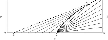
The solution in the upper domain ( $\hat{z}>\hat{z}_{\text{R}}$
) matches the lower domain (
$\hat{z}>\hat{z}_{\text{R}}$
) matches the lower domain ( $\hat{z}<\hat{z}_{\text{R}}$
) along the no-mean-flow line
$\hat{z}<\hat{z}_{\text{R}}$
) along the no-mean-flow line ${\it\psi}={\it\psi}_{\text{R}}$
. As
${\it\psi}={\it\psi}_{\text{R}}$
. As $F^{\prime }({\it\phi}_{\text{R}})=0$
, the
$F^{\prime }({\it\phi}_{\text{R}})=0$
, the ${\it\phi}_{\text{R}}$
characteristic lies horizontally between points
${\it\phi}_{\text{R}}$
characteristic lies horizontally between points $\text{C}$
and
$\text{C}$
and $\text{A}$
and gives concentration
$\text{A}$
and gives concentration ${\it\phi}={\it\phi}_{\text{R}}$
, whilst (2.28) governs the concentration between
${\it\phi}={\it\phi}_{\text{R}}$
, whilst (2.28) governs the concentration between $\text{A}$
and
$\text{A}$
and $\text{F}$
. A characteristic of concentration
$\text{F}$
. A characteristic of concentration ${\it\phi}^{o}$
emanates into the upper region from each point between
${\it\phi}^{o}$
emanates into the upper region from each point between $\text{F}$
and
$\text{F}$
and $\text{A}$
 $$\begin{eqnarray}\displaystyle {\it\psi}={\it\psi}_{\text{R}}-F^{\prime }({\it\phi}^{o})({\it\xi}-{\it\xi}_{\text{F}\text{A}}({\it\phi})), & & \displaystyle\end{eqnarray}$$
with ${\it\phi}\in [{\it\phi}_{\text{E}},{\it\phi}_{\text{R}}]$
implying that
${\it\phi}\in [{\it\phi}_{\text{E}},{\it\phi}_{\text{R}}]$
implying that ${\it\phi}_{\text{R}}^{o}\leqslant {\it\phi}^{o}\leqslant 1$
. The
${\it\phi}_{\text{R}}^{o}\leqslant {\it\phi}^{o}\leqslant 1$
. The ${\it\phi}_{\text{R}}^{o}$
characteristic originates from
${\it\phi}_{\text{R}}^{o}$
characteristic originates from $\text{A}$
, whilst the
$\text{A}$
, whilst the ${\it\phi}=1$
characteristic originates from
${\it\phi}=1$
characteristic originates from $\text{F}$
. All the characteristics form a compression wave
$\text{F}$
. All the characteristics form a compression wave $\text{F}\text{G}\text{A}\text{F}$
(Whitham Reference Whitham1974; Rhee et al.
Reference Rhee, Aris and Amundson1986); each characteristic has a steeper gradient than the characteristic immediately to its left, as shown in figure 11. This is the upper portion of the ‘tail’ region. The ‘lens’ region is formed from an expansion fan
$\text{F}\text{G}\text{A}\text{F}$
(Whitham Reference Whitham1974; Rhee et al.
Reference Rhee, Aris and Amundson1986); each characteristic has a steeper gradient than the characteristic immediately to its left, as shown in figure 11. This is the upper portion of the ‘tail’ region. The ‘lens’ region is formed from an expansion fan $\text{A}\text{G}\text{B}\text{C}\text{A}$
centred at
$\text{A}\text{G}\text{B}\text{C}\text{A}$
centred at $\text{A}$
whose characteristics are given by (2.17) with
$\text{A}$
whose characteristics are given by (2.17) with ${\it\phi}_{\text{R}}\leqslant {\it\phi}\leqslant {\it\phi}_{\text{R}}^{oo}$
. These rarefaction characteristics collide with the compression wave characteristics (2.30) to form a shock
${\it\phi}_{\text{R}}\leqslant {\it\phi}\leqslant {\it\phi}_{\text{R}}^{oo}$
. These rarefaction characteristics collide with the compression wave characteristics (2.30) to form a shock $\text{A}\text{G}$
. A full derivation of the governing equations for the shock is provided in appendix B. The shock coordinates are given implicitly given by
$\text{A}\text{G}$
. A full derivation of the governing equations for the shock is provided in appendix B. The shock coordinates are given implicitly given by
 $$\begin{eqnarray}\displaystyle {\it\xi}_{\text{A}\text{G}}({\it\phi}_{left},{\it\phi}_{right}) & = & \displaystyle {\displaystyle \frac{F^{\prime }({\it\phi}_{left})\tilde{{\it\xi}}_{\text{F}\text{A}}({\it\phi}_{left})-F^{\prime }({\it\phi}_{right}){\it\xi}_{\text{F}}}{F^{\prime }({\it\phi}_{left})-F^{\prime }({\it\phi}_{right})}},\end{eqnarray}$$
 $$\begin{eqnarray}\displaystyle {\it\psi}_{\text{A}\text{G}}({\it\phi}_{left},{\it\phi}_{right}) & = & \displaystyle {\it\psi}_{\text{R}}-{\displaystyle \frac{F^{\prime }({\it\phi}_{left})F^{\prime }({\it\phi}_{right})}{F^{\prime }({\it\phi}_{left})-F^{\prime }({\it\phi}_{right})}}(\tilde{{\it\xi}}_{\text{F}\text{A}}({\it\phi}_{left})-{\it\xi}_{\text{F}}),\end{eqnarray}$$ ${\it\xi}_{\text{F}\text{A}}({\it\phi})=\tilde{{\it\xi}}_{\text{F}\text{A}}({\it\phi}^{o})$
, and concentrations
${\it\xi}_{\text{F}\text{A}}({\it\phi})=\tilde{{\it\xi}}_{\text{F}\text{A}}({\it\phi}^{o})$
, and concentrations ${\it\phi}_{left}$
and
${\it\phi}_{left}$
and ${\it\phi}_{right}$
on the left (upstream) and right (downstream) sides of the shock are related by
${\it\phi}_{right}$
on the left (upstream) and right (downstream) sides of the shock are related by  $$\begin{eqnarray}\displaystyle {\displaystyle \frac{\text{d}{\it\phi}_{right}}{\text{d}{\it\phi}_{left}}} & = & \displaystyle {\displaystyle \frac{F({\it\phi}_{left})-F({\it\phi}_{right})-({\it\phi}_{left}-{\it\phi}_{right})F^{\prime }({\it\phi}_{right})}{F({\it\phi}_{left})-F({\it\phi}_{right})-({\it\phi}_{left}-{\it\phi}_{right})F^{\prime }({\it\phi}_{left})}}\nonumber\\ \displaystyle & & \displaystyle \times \left[{\displaystyle \frac{F^{\prime }({\it\phi}_{right})F^{\prime \prime }({\it\phi}_{left})}{F^{\prime }({\it\phi}_{left})F^{\prime \prime }({\it\phi}_{right})}}-{\displaystyle \frac{F^{\prime }({\it\phi}_{left})-F^{\prime }({\it\phi}_{right})}{F^{\prime \prime }({\it\phi}_{right})}}{\displaystyle \frac{\tilde{{\it\xi}}_{\text{F}\text{A}}^{\prime }({\it\phi}_{left})}{\tilde{{\it\xi}}_{\text{F}\text{A}}({\it\phi}_{left})-{\it\xi}_{\text{F}}}}\right].\end{eqnarray}$$
The shock entropy condition (Oleinik Reference Oleinik1959; Rhee et al.
Reference Rhee, Aris and Amundson1986; Gajjar & Gray Reference Gajjar and Gray2014) requires that $\text{A}\text{G}$
must initially start tangential to the rarefaction fan, and as
$\text{A}\text{G}$
must initially start tangential to the rarefaction fan, and as ${\it\phi}_{left}={\it\phi}_{\text{R}}^{o}$
at point
${\it\phi}_{left}={\it\phi}_{\text{R}}^{o}$
at point $\text{A}$
, (1.9) implies that
$\text{A}$
, (1.9) implies that ${\it\phi}_{right}=({\it\phi}_{\text{R}}^{o})^{o}={\it\phi}_{\text{R}}^{oo}$
at this point. The relationship between
${\it\phi}_{right}=({\it\phi}_{\text{R}}^{o})^{o}={\it\phi}_{\text{R}}^{oo}$
at this point. The relationship between ${\it\phi}_{\text{R}}$
,
${\it\phi}_{\text{R}}$
, ${\it\phi}_{\text{R}}^{o}$
and
${\it\phi}_{\text{R}}^{o}$
and ${\it\phi}_{\text{R}}^{oo}$
is illustrated in figure 8. Equation (2.32) may be numerically integrated from
${\it\phi}_{\text{R}}^{oo}$
is illustrated in figure 8. Equation (2.32) may be numerically integrated from ${\it\phi}_{left}={\it\phi}_{\text{R}}^{o}$
to
${\it\phi}_{left}={\it\phi}_{\text{R}}^{o}$
to ${\it\phi}_{left}=1$
to give
${\it\phi}_{left}=1$
to give ${\it\phi}_{right}={\it\phi}_{\text{G}}$
at point
${\it\phi}_{right}={\it\phi}_{\text{G}}$
at point $\text{G}$
and the coordinates
$\text{G}$
and the coordinates $({\it\xi}_{\text{G}},{\it\psi}_{\text{G}})$
of point
$({\it\xi}_{\text{G}},{\it\psi}_{\text{G}})$
of point $\text{G}$
are given by (2.31). Shock
$\text{G}$
are given by (2.31). Shock $\text{G}\text{B}$
separates the upstream region of pure small particles (
$\text{G}\text{B}$
separates the upstream region of pure small particles ( ${\it\phi}^{-}=1$
) from the rarefaction fan in the ‘lens’ region (
${\it\phi}^{-}=1$
) from the rarefaction fan in the ‘lens’ region ( ${\it\phi}^{+}={\it\phi}$
). Combining (2.7) and (2.17) using the chain rule shows that
${\it\phi}^{+}={\it\phi}$
). Combining (2.7) and (2.17) using the chain rule shows that $\text{G}\text{B}$
satisfies
$\text{G}\text{B}$
satisfies
 $$\begin{eqnarray}\displaystyle {\displaystyle \frac{\text{d}}{\text{d}{\it\phi}}}[(F({\it\phi})+(1-{\it\phi})F^{\prime }({\it\phi}))\,({\it\xi}-{\it\xi}_{\text{A}})]=0. & & \displaystyle\end{eqnarray}$$
The shock starts from point $\text{G}$
, and hence (2.33) can be integrated to give
$\text{G}$
, and hence (2.33) can be integrated to give
 $$\begin{eqnarray}\displaystyle {\it\xi}_{\text{G}\text{B}} & = & \displaystyle {\it\xi}_{\text{A}}+{\displaystyle \frac{F({\it\phi}_{\text{G}})+(1-{\it\phi}_{\text{G}})F^{\prime }({\it\phi}_{\text{G}})}{F({\it\phi})+(1-{\it\phi})F^{\prime }({\it\phi})}}\left({\it\xi}_{\text{G}}-{\it\xi}_{\text{A}}\right),\end{eqnarray}$$
 $$\begin{eqnarray}\displaystyle {\it\psi}_{\text{G}\text{B}} & = & \displaystyle {\it\psi}_{\text{R}}-F^{\prime }({\it\phi})({\it\xi}_{\text{G}\text{B}}({\it\phi})-{\it\xi}_{\text{A}}),\end{eqnarray}$$ ${\it\phi}\in [{\it\phi}_{\text{B}},{\it\phi}_{\text{G}}]$
. A final shock
${\it\phi}\in [{\it\phi}_{\text{B}},{\it\phi}_{\text{G}}]$
. A final shock $\text{B}\text{C}$
satisfying (2.19) separates the downstream region of large particles (
$\text{B}\text{C}$
satisfying (2.19) separates the downstream region of large particles ( ${\it\phi}^{+}=0$
) from the rarefaction fan (
${\it\phi}^{+}=0$
) from the rarefaction fan ( ${\it\phi}^{-}={\it\phi}$
). Shock
${\it\phi}^{-}={\it\phi}$
). Shock $\text{B}\text{C}$
must meet the no-mean-flow line at
$\text{B}\text{C}$
must meet the no-mean-flow line at $\text{C}$
, where
$\text{C}$
, where ${\it\phi}={\it\phi}_{\text{R}}$
, and since
${\it\phi}={\it\phi}_{\text{R}}$
, and since ${\it\xi}_{\text{C}}-{\it\xi}_{\text{A}}$
is given by (2.26), equation (2.19) can be integrated to give
${\it\xi}_{\text{C}}-{\it\xi}_{\text{A}}$
is given by (2.26), equation (2.19) can be integrated to give  $$\begin{eqnarray}\displaystyle {\it\xi}_{\text{B}\text{C}} & = & \displaystyle {\it\xi}_{\text{A}}-{\displaystyle \frac{\mathscr{G}}{F({\it\phi})-{\it\phi}F^{\prime }({\it\phi})}}={\it\xi}_{\text{A}}-{\displaystyle \frac{\mathscr{G}}{A_{{\it\gamma}}{\it\phi}^{2}(1+{\it\gamma}-2{\it\gamma}{\it\phi})}},\end{eqnarray}$$
 $$\begin{eqnarray}\displaystyle {\it\psi}_{\text{B}\text{C}} & = & \displaystyle {\it\psi}_{\text{R}}-{\displaystyle \frac{F^{\prime }({\it\phi})\mathscr{G}}{F({\it\phi})-{\it\phi}F^{\prime }({\it\phi})}},\end{eqnarray}$$ ${\it\phi}\in [{\it\phi}_{\text{R}},{\it\phi}_{\text{B}}]$
and
${\it\phi}\in [{\it\phi}_{\text{R}},{\it\phi}_{\text{B}}]$
and  $$\begin{eqnarray}\displaystyle \mathscr{G}=({\it\xi}_{\text{C}}-{\it\xi}_{\text{A}})F({\it\phi}_{\text{R}})={\displaystyle \frac{{\it\xi}_{\text{C}}-{\it\xi}_{\text{A}}}{4}}={\displaystyle \frac{{\it\psi}_{\text{R}}{\it\gamma}^{2}}{A_{{\it\gamma}}}}\left({\displaystyle \frac{4}{(2{\it\gamma}-1)({\it\gamma}^{2}-{\it\gamma}+1)^{4}}}\right)^{1/3}. & & \displaystyle\end{eqnarray}$$
The shock reaches the top of the ‘lens’ at point $\text{B}$
where
$\text{B}$
where ${\it\psi}=0$
, and hence (2.35) determines both
${\it\psi}=0$
, and hence (2.35) determines both ${\it\phi}_{\text{B}}$
and
${\it\phi}_{\text{B}}$
and ${\it\xi}_{\text{B}}$
.
${\it\xi}_{\text{B}}$
.
A requirement for the ‘lens-tail’ solution to form is that point $\text{E}$
must reside in the lower domain, which occurs when
$\text{E}$
must reside in the lower domain, which occurs when ${\it\phi}_{\text{E}}<{\it\phi}_{\text{R}}$
. Instead, if
${\it\phi}_{\text{E}}<{\it\phi}_{\text{R}}$
. Instead, if ${\it\phi}_{\text{E}}>{\it\phi}_{\text{R}}$
, then point
${\it\phi}_{\text{E}}>{\it\phi}_{\text{R}}$
, then point $\text{E}$
would lie in the upper domain and shock
$\text{E}$
would lie in the upper domain and shock $\text{D}\text{E}$
would continue up to the no-mean-flow line, forming the non-convex ‘lens’ structure of § 2.2. The transition between the ‘lens’ solution and the ‘lens-tail’ solution thus occurs when point
$\text{D}\text{E}$
would continue up to the no-mean-flow line, forming the non-convex ‘lens’ structure of § 2.2. The transition between the ‘lens’ solution and the ‘lens-tail’ solution thus occurs when point $\text{E}$
lies on the no-mean-flow line
$\text{E}$
lies on the no-mean-flow line ${\it\psi}={\it\psi}_{\text{R}}$
, i.e. when
${\it\psi}={\it\psi}_{\text{R}}$
, i.e. when ${\it\phi}_{\text{R}}={\it\phi}_{\text{E}}$
. The definition
${\it\phi}_{\text{R}}={\it\phi}_{\text{E}}$
. The definition $F^{\prime }({\it\phi}_{\text{R}})=0$
implies that for the cubic flux (1.5)
$F^{\prime }({\it\phi}_{\text{R}})=0$
implies that for the cubic flux (1.5)
 $$\begin{eqnarray}\displaystyle {\it\phi}_{\text{R}}={\displaystyle \frac{1+{\it\gamma}\pm \sqrt{{\it\gamma}^{2}-{\it\gamma}+1}}{3{\it\gamma}}}, & & \displaystyle\end{eqnarray}$$
and equating this with ${\it\phi}_{\text{E}}$
(1.10b
) gives the quadratic equation
${\it\phi}_{\text{E}}$
(1.10b
) gives the quadratic equation
 $$\begin{eqnarray}\displaystyle 5{\it\gamma}^{2}-5{\it\gamma}+1=0. & & \displaystyle\end{eqnarray}$$
As the cubic flux (1.5) is non-convex when ${\it\gamma}>0.5$
, the transition between the non-convex ‘lens’ and ‘lens-tail’ solutions takes place at the larger of the two roots of (2.38), namely
${\it\gamma}>0.5$
, the transition between the non-convex ‘lens’ and ‘lens-tail’ solutions takes place at the larger of the two roots of (2.38), namely
 $$\begin{eqnarray}\displaystyle {\it\gamma}={\it\Gamma}=(5+\sqrt{5})/10. & & \displaystyle\end{eqnarray}$$
2.4 Solution in physical coordinates
Following Thornton & Gray (Reference Thornton and Gray2008), transformations (2.1) and (2.4) from $(x,z)$
to
$(x,z)$
to $({\it\xi},{\it\psi})$
coordinates mean that the steady-state structures shown in figure 10 describe all of the breaking size-segregation waves that develop under steady uniform flow. They are valid for waves that exist between all vertical heights
$({\it\xi},{\it\psi})$
coordinates mean that the steady-state structures shown in figure 10 describe all of the breaking size-segregation waves that develop under steady uniform flow. They are valid for waves that exist between all vertical heights $H_{down}$
and
$H_{down}$
and $H_{up}$
, for any constant segregation number
$H_{up}$
, for any constant segregation number $S_{r}$
and for any monotonically increasing velocity profile
$S_{r}$
and for any monotonically increasing velocity profile $u(z)$
. For example, consider the simple linear velocity profile,
$u(z)$
. For example, consider the simple linear velocity profile,
 $$\begin{eqnarray}\displaystyle u={\it\alpha}+2(1-{\it\alpha})z,\quad 0\leqslant {\it\alpha}<1, & & \displaystyle\end{eqnarray}$$
where ${\it\alpha}$
is the parameter that controls the amount of shear across the layer. The case of
${\it\alpha}$
is the parameter that controls the amount of shear across the layer. The case of ${\it\alpha}=0$
represents simple shear with zero basal velocity, whilst
${\it\alpha}=0$
represents simple shear with zero basal velocity, whilst ${\it\alpha}=1$
corresponds to plug flow. Not only is this the simplest non-trivial velocity field that highlights all the major features of the breaking-wave structure, but it is also a good leading-order approximation to the velocity field measured in the (shallow) moving-bed flume experiments of § 1.1. From (1.13), the breaking wave travels downstream with velocity
${\it\alpha}=1$
corresponds to plug flow. Not only is this the simplest non-trivial velocity field that highlights all the major features of the breaking-wave structure, but it is also a good leading-order approximation to the velocity field measured in the (shallow) moving-bed flume experiments of § 1.1. From (1.13), the breaking wave travels downstream with velocity
 $$\begin{eqnarray}\displaystyle u_{wave}={\it\alpha}+(1-{\it\alpha})(H_{up}+H_{down}), & & \displaystyle\end{eqnarray}$$
and so the relative downstream velocity $\hat{u}$
becomes
$\hat{u}$
becomes
 $$\begin{eqnarray}\displaystyle \hat{u} =(1-{\it\alpha})(H_{up}-H_{down})(2\hat{z}-1). & & \displaystyle\end{eqnarray}$$
The no-mean-flow line $\hat{z}_{\text{R}}=1/2$
lies halfway between the vertical heights
$\hat{z}_{\text{R}}=1/2$
lies halfway between the vertical heights $H_{down}$
and
$H_{down}$
and $H_{up}$
in untransformed variables. Transformation (2.4) means that
$H_{up}$
in untransformed variables. Transformation (2.4) means that $z$
and
$z$
and ${\it\psi}$
have a quadratic relation,
${\it\psi}$
have a quadratic relation,
 $$\begin{eqnarray}\displaystyle {\it\psi}=(1-{\it\alpha})(H_{up}-H_{down})(\hat{z}^{2}-\hat{z}), & & \displaystyle\end{eqnarray}$$
with the transformed no-mean-flow line ${\it\psi}_{\text{R}}=-(1-{\it\alpha})(H_{up}-H_{down})/4$
. Inverting equation (2.43) gives
${\it\psi}_{\text{R}}=-(1-{\it\alpha})(H_{up}-H_{down})/4$
. Inverting equation (2.43) gives $\hat{z}$
as a function of
$\hat{z}$
as a function of ${\it\psi}$
, with the positive and negative roots for the upper and lower regions, respectively. Figure 12 shows the steady breaking waves in physical coordinates for linear shear with
${\it\psi}$
, with the positive and negative roots for the upper and lower regions, respectively. Figure 12 shows the steady breaking waves in physical coordinates for linear shear with ${\it\alpha}=0.5$
,
${\it\alpha}=0.5$
, $S_{r}=1$
,
$S_{r}=1$
, $H_{up}=0.9$
and
$H_{up}=0.9$
and $H_{down}=0.1$
for
$H_{down}=0.1$
for ${\it\gamma}=0.35$
,
${\it\gamma}=0.35$
, $0.65$
and
$0.65$
and $0.9$
in (a), (b) and (c) respectively.
$0.9$
in (a), (b) and (c) respectively.
The breaking wave that develops between $H_{up}=0.9$
and
$H_{up}=0.9$
and $H_{down}=0.1$
is shown in physical coordinates
$H_{down}=0.1$
is shown in physical coordinates $(x,z)$
in a frame translating with velocity
$(x,z)$
in a frame translating with velocity $u_{wave}$
(1.13). The bulk velocity
$u_{wave}$
(1.13). The bulk velocity $u(z)$
follows a linear shear profile (2.40) with
$u(z)$
follows a linear shear profile (2.40) with ${\it\alpha}=0.5$
. The three different structures that arise for the asymmetric cubic flux (1.5) with
${\it\alpha}=0.5$
. The three different structures that arise for the asymmetric cubic flux (1.5) with $S_{r}=1$
are shown in (a–c) for
$S_{r}=1$
are shown in (a–c) for ${\it\gamma}=0.35$
,
${\it\gamma}=0.35$
, $0.65$
and
$0.65$
and $0.9$
, respectively. The asymmetry in the large and small particle velocities that result from the asymmetric flux function causes point
$0.9$
, respectively. The asymmetry in the large and small particle velocities that result from the asymmetric flux function causes point $\text{B}$
to be swept further downstream in the two ‘lens’-like structures (a) and (b) compared to the symmetric quadratic flux shown in figure 9(e). These asymmetric velocities are even more significant in (c), where the slow rise rate of large particles surrounded by many fines means that some large particles are swept a long way upstream before recirculating. This results in the ‘tail’ region
$\text{B}$
to be swept further downstream in the two ‘lens’-like structures (a) and (b) compared to the symmetric quadratic flux shown in figure 9(e). These asymmetric velocities are even more significant in (c), where the slow rise rate of large particles surrounded by many fines means that some large particles are swept a long way upstream before recirculating. This results in the ‘tail’ region $\text{E}\text{F}\text{G}\text{A}\text{E}$
. The concentration map reflects how only a small number of large particles recirculate through this region. Most large particles still rise at a moderate velocity, and recirculate in the ‘lens’ region.
$\text{E}\text{F}\text{G}\text{A}\text{E}$
. The concentration map reflects how only a small number of large particles recirculate through this region. Most large particles still rise at a moderate velocity, and recirculate in the ‘lens’ region.

2.5 Comparison with solution for the quadratic flux
The asymmetric cubic flux function (1.5) leads to a number of differences in the structures shown in figure 12 and that of the quadratic flux function (1.2) shown in figure 9(e). The two ‘lens’-like structures in figure 12(a,b) have a strong similarity to the symmetric ‘lens’ structure. As the normalisation of the flux function (2.8) implies that (2.21) is independent of ${\it\gamma}$
, the ‘lens’ length is identical to the quadratic ‘lens’ length
${\it\gamma}$
, the ‘lens’ length is identical to the quadratic ‘lens’ length $(1-{\it\alpha})(H_{up}-H_{down})^{2}/S_{r}$
. However, with an asymmetric flux, the ‘lens’ structures have no rotational symmetry. The asymmetry also means the maximum rise velocity of large particles is less than the maximum percolation velocity of fines, causing point
$(1-{\it\alpha})(H_{up}-H_{down})^{2}/S_{r}$
. However, with an asymmetric flux, the ‘lens’ structures have no rotational symmetry. The asymmetry also means the maximum rise velocity of large particles is less than the maximum percolation velocity of fines, causing point $\text{B}$
to lie further downstream. When
$\text{B}$
to lie further downstream. When ${\it\Gamma}<{\it\gamma}\leqslant 1$
, a few large particles surrounded by many fines rise very slowly, and so are swept a long way downstream before recirculating. This causes the additional ‘tail’-like region, and substantially increases the length of the breaking wave. The colour map shows how the concentration in the ‘tail’ is very similar to
${\it\Gamma}<{\it\gamma}\leqslant 1$
, a few large particles surrounded by many fines rise very slowly, and so are swept a long way downstream before recirculating. This causes the additional ‘tail’-like region, and substantially increases the length of the breaking wave. The colour map shows how the concentration in the ‘tail’ is very similar to ${\it\phi}=1$
of the surrounding region of pure small particles, reflecting the very small number of large particles that circulate slowly through this region. Most of the large particles still rise at a moderate speed through the ‘lens’ region; however, the small particles percolate down very quickly. This leaves a higher concentration of coarse grains in the middle of the ‘lens’, shown by a stronger green hue. Interestingly, the length of this ‘lens’ region in the ‘lens-tail’ structure remains very close to the length of the ‘lens’ structures. Comparing (2.26) with (2.16) shows that the length of the ‘lens’ within the ‘lens-tail’ structure is, at most, only 9 % less than the length of the ‘lens’ structure.
${\it\phi}=1$
of the surrounding region of pure small particles, reflecting the very small number of large particles that circulate slowly through this region. Most of the large particles still rise at a moderate speed through the ‘lens’ region; however, the small particles percolate down very quickly. This leaves a higher concentration of coarse grains in the middle of the ‘lens’, shown by a stronger green hue. Interestingly, the length of this ‘lens’ region in the ‘lens-tail’ structure remains very close to the length of the ‘lens’ structures. Comparing (2.26) with (2.16) shows that the length of the ‘lens’ within the ‘lens-tail’ structure is, at most, only 9 % less than the length of the ‘lens’ structure.
3 Recirculating particle motion through the breaking wave
The recirculating motion of the grains can be understood by examining the particle paths as they pass through the breaking wave. Following Thornton et al. (Reference Thornton, Gray and Hogg2006) and Thornton & Gray (Reference Thornton and Gray2008), the particle paths of the large (superscript $l$
) and small grains (superscript
$l$
) and small grains (superscript $s$
) are given by
$s$
) are given by
 $$\begin{eqnarray}\displaystyle {\displaystyle \frac{\text{d}x^{{\it\nu}}}{\text{d}t}}=u^{{\it\nu}},\quad {\displaystyle \frac{\text{d}z^{{\it\nu}}}{\text{d}t}}=w^{{\it\nu}},\quad ({\it\nu}=l,s). & & \displaystyle\end{eqnarray}$$
The normal constituent velocities $w^{{\it\nu}}$
are given by (1.3) and the downstream constituent velocities are assumed to be equal to the downstream bulk velocity (1.11),
$w^{{\it\nu}}$
are given by (1.3) and the downstream constituent velocities are assumed to be equal to the downstream bulk velocity (1.11), $u^{s}=u^{l}=u$
. Eliminating the time dependence from (3.1) and employing the non-dimensionalisation (2.1) gives the non-dimensional particle paths
$u^{s}=u^{l}=u$
. Eliminating the time dependence from (3.1) and employing the non-dimensionalisation (2.1) gives the non-dimensional particle paths
 $$\begin{eqnarray}\displaystyle \hat{u} (\hat{z}){\displaystyle \frac{\text{d}\hat{z}^{{\it\nu}}}{\text{d}\hat{x}^{{\it\nu}}}}={\hat{w}}^{{\it\nu}}({\it\phi}),\quad ({\it\nu}=l,s), & & \displaystyle\end{eqnarray}$$
which simplify further in velocity-averaged coordinates (2.4) to give
 $$\begin{eqnarray}\displaystyle {\displaystyle \frac{\text{d}{\it\psi}^{l}}{\text{d}{\it\xi}^{l}}}={\displaystyle \frac{F({\it\phi})}{1-{\it\phi}}},\quad {\displaystyle \frac{\text{d}{\it\psi}^{s}}{\text{d}{\it\xi}^{s}}}=-{\displaystyle \frac{F({\it\phi})}{{\it\phi}}}. & & \displaystyle\end{eqnarray}$$
The concentration fields derived in § 2 can be used with (3.3) to calculate the particle paths through each of the breaking-wave structures.
3.1 Recirculation through the ‘lens’ structures
First consider the recirculation through a breaking wave with a convex ‘lens’ structure when ${\it\gamma}\leqslant 0.5$
. Suppose a small particle starts at a height
${\it\gamma}\leqslant 0.5$
. Suppose a small particle starts at a height $\hat{z}_{enter}^{s}>\hat{z}_{\text{R}}$
, equivalent to transformed height
$\hat{z}_{enter}^{s}>\hat{z}_{\text{R}}$
, equivalent to transformed height ${\it\psi}_{enter}^{s}$
. The small grains are moving faster than the breaking wave in the upper region, and so they are swept downstream to the right before crossing
${\it\psi}_{enter}^{s}$
. The small grains are moving faster than the breaking wave in the upper region, and so they are swept downstream to the right before crossing $\text{A}\text{B}$
and entering the ‘lens’ at downstream distance
$\text{A}\text{B}$
and entering the ‘lens’ at downstream distance
 $$\begin{eqnarray}\displaystyle {\it\xi}_{enter}^{s}={\it\xi}_{\text{A}}+{\displaystyle \frac{{\it\psi}_{enter}^{s}-{\it\psi}_{\text{R}}}{F^{\prime }(1)}}. & & \displaystyle\end{eqnarray}$$
Although the local small particle velocity is given by (3.3b
), the local concentration changes through the rarefaction fan $\text{A}\text{B}\text{C}\text{A}$
according to characteristics (2.17). These characteristics may be differentiated with respect to
$\text{A}\text{B}\text{C}\text{A}$
according to characteristics (2.17). These characteristics may be differentiated with respect to ${\it\phi}$
as in (2.13), whilst the chain rule may be used to write the small particle velocity (3.3b
) in a similar manner to (2.12). Combining these equations shows that the small particle motion through the upper part of the ‘lens’ is governed by ODE (2.19), with
${\it\phi}$
as in (2.13), whilst the chain rule may be used to write the small particle velocity (3.3b
) in a similar manner to (2.12). Combining these equations shows that the small particle motion through the upper part of the ‘lens’ is governed by ODE (2.19), with ${\it\xi}^{s}$
instead of
${\it\xi}^{s}$
instead of ${\it\xi}$
. As the small particle enters the ‘lens’ at
${\it\xi}$
. As the small particle enters the ‘lens’ at ${\it\xi}_{enter}^{s}$
(3.4) when
${\it\xi}_{enter}^{s}$
(3.4) when ${\it\phi}=1$
, the motion through
${\it\phi}=1$
, the motion through $\text{A}\text{B}\text{C}\text{A}$
is given by
$\text{A}\text{B}\text{C}\text{A}$
is given by
 $$\begin{eqnarray}\displaystyle {\it\xi}^{s}={\it\xi}_{\text{A}}+{\displaystyle \frac{{\it\psi}_{enter}^{s}-{\it\psi}_{\text{R}}}{F({\it\phi})-{\it\phi}F^{\prime }({\it\phi})}}, & & \displaystyle\end{eqnarray}$$
with ${\it\phi}\in [{\it\phi}_{\text{R}},1]$
. The small particle continues along this path until it crosses the no-mean-flow line
${\it\phi}\in [{\it\phi}_{\text{R}},1]$
. The small particle continues along this path until it crosses the no-mean-flow line $\text{A}\text{C}$
at
$\text{A}\text{C}$
at
 $$\begin{eqnarray}\displaystyle {\it\xi}_{\text{A}\text{C}}^{s}={\it\xi}_{\text{A}}+{\displaystyle \frac{{\it\psi}_{enter}^{s}-{\it\psi}_{\text{R}}}{F({\it\phi}_{\text{R}})}}={\it\xi}_{\text{A}}+4({\it\psi}_{enter}^{s}-{\it\psi}_{\text{R}}), & & \displaystyle\end{eqnarray}$$
with the last equation a result of the normalisation (2.8). The motion through the lower region $\text{C}\text{D}\text{A}\text{C}$
is similarly governed by velocity (3.3b
) and characteristics (2.9), which combine to give the differential equation
$\text{C}\text{D}\text{A}\text{C}$
is similarly governed by velocity (3.3b
) and characteristics (2.9), which combine to give the differential equation
 $$\begin{eqnarray}\displaystyle {\displaystyle \frac{\text{d}}{\text{d}{\it\phi}}}[(F({\it\phi})-{\it\phi}F^{\prime }({\it\phi}))\,({\it\xi}^{s}-{\it\xi}_{\text{C}})]=0. & & \displaystyle\end{eqnarray}$$
Since the small particle crosses the no-mean-flow line at ${\it\xi}^{s}={\it\xi}_{\text{A}\text{C}}^{s}$
when
${\it\xi}^{s}={\it\xi}_{\text{A}\text{C}}^{s}$
when ${\it\phi}={\it\phi}_{\text{R}}$
, equations (2.21), (3.6) and (3.7) imply that the motion through the lower region
${\it\phi}={\it\phi}_{\text{R}}$
, equations (2.21), (3.6) and (3.7) imply that the motion through the lower region $\text{C}\text{D}\text{A}\text{C}$
is given by
$\text{C}\text{D}\text{A}\text{C}$
is given by
 $$\begin{eqnarray}\displaystyle {\it\xi}^{s}={\it\xi}_{\text{C}}+{\displaystyle \frac{{\it\psi}_{enter}^{s}}{F({\it\phi})-{\it\phi}F^{\prime }({\it\phi})}}, & & \displaystyle\end{eqnarray}$$
with ${\it\phi}\in [{\it\phi}_{\text{D}\text{A}}^{s},{\it\phi}_{\text{R}}]$
. The small particle exits the breaking wave across
${\it\phi}\in [{\it\phi}_{\text{D}\text{A}}^{s},{\it\phi}_{\text{R}}]$
. The small particle exits the breaking wave across $\text{D}\text{A}$
, with equations (2.9), (2.15) and (3.8) giving both the concentration
$\text{D}\text{A}$
, with equations (2.9), (2.15) and (3.8) giving both the concentration ${\it\phi}_{\text{D}\text{A}}^{s}$
and the exit height
${\it\phi}_{\text{D}\text{A}}^{s}$
and the exit height ${\it\psi}_{\text{D}\text{A}}^{s}$
.
${\it\psi}_{\text{D}\text{A}}^{s}$
.
Similarly, consider a large particle that starts in the lower region at a height $\hat{z}^{l}=\hat{z}_{enter}^{l}<\hat{z}_{\text{R}}$
, corresponding to
$\hat{z}^{l}=\hat{z}_{enter}^{l}<\hat{z}_{\text{R}}$
, corresponding to ${\it\psi}^{l}={\it\psi}_{enter}^{l}$
. The large particles initially move slower than the breaking wave, and so are swept upstream to the left until they meet
${\it\psi}^{l}={\it\psi}_{enter}^{l}$
. The large particles initially move slower than the breaking wave, and so are swept upstream to the left until they meet $\text{C}\text{D}$
at distance
$\text{C}\text{D}$
at distance
 $$\begin{eqnarray}\displaystyle {\it\xi}_{enter}^{l}={\it\xi}_{\text{C}}+{\displaystyle \frac{{\it\psi}_{\text{R}}-{\it\psi}_{enter}^{l}}{F^{\prime }(0)}}. & & \displaystyle\end{eqnarray}$$
The concentration within the lower part of the ‘lens’ $\text{C}\text{D}\text{A}\text{C}$
is governed by characteristics (2.9) whilst the local velocity is given by (3.3a
); these combine to give differential equation (2.14) with
$\text{C}\text{D}\text{A}\text{C}$
is governed by characteristics (2.9) whilst the local velocity is given by (3.3a
); these combine to give differential equation (2.14) with ${\it\xi}^{l}$
replacing
${\it\xi}^{l}$
replacing ${\it\xi}$
. With the initial condition
${\it\xi}$
. With the initial condition ${\it\phi}=0$
at
${\it\phi}=0$
at ${\it\xi}^{l}={\it\xi}_{enter}^{l}$
, the large particle path through
${\it\xi}^{l}={\it\xi}_{enter}^{l}$
, the large particle path through $\text{C}\text{D}\text{A}\text{C}$
is given by
$\text{C}\text{D}\text{A}\text{C}$
is given by
 $$\begin{eqnarray}\displaystyle {\it\xi}^{l}={\it\xi}_{\text{C}}+{\displaystyle \frac{{\it\psi}_{\text{R}}-{\it\psi}_{enter}^{l}}{F({\it\phi})+(1-{\it\phi})F^{\prime }({\it\phi})}}. & & \displaystyle\end{eqnarray}$$
Each large particle crosses the no-mean-flow line $\text{A}\text{C}$
at distance
$\text{A}\text{C}$
at distance
 $$\begin{eqnarray}\displaystyle {\it\xi}_{\text{A}\text{C}}^{l}={\it\xi}_{\text{C}}+{\displaystyle \frac{{\it\psi}_{\text{R}}-{\it\psi}_{enter}^{l}}{F({\it\phi}_{\text{R}})}}={\it\xi}_{\text{C}}+4({\it\psi}_{\text{R}}-{\it\psi}_{enter}^{l}). & & \displaystyle\end{eqnarray}$$
In the upper part of the ‘lens’, characteristics (2.17) govern the concentration at a point $({\it\xi},{\it\psi})$
, and can be combined with (3.3a
) to give a governing differential equation that resembles (2.14)
$({\it\xi},{\it\psi})$
, and can be combined with (3.3a
) to give a governing differential equation that resembles (2.14)
 $$\begin{eqnarray}\displaystyle {\displaystyle \frac{\text{d}}{\text{d}{\it\phi}}}[(F({\it\phi})+(1-{\it\phi})F^{\prime }({\it\phi}))\,({\it\xi}^{l}-{\it\xi}_{\text{A}})]=0. & & \displaystyle\end{eqnarray}$$
The initial condition that ${\it\phi}={\it\phi}_{\text{R}}$
at
${\it\phi}={\it\phi}_{\text{R}}$
at ${\it\xi}^{l}={\it\xi}_{\text{A}\text{C}}^{l}$
, along with (2.21) and (3.11) give the large particle path through
${\it\xi}^{l}={\it\xi}_{\text{A}\text{C}}^{l}$
, along with (2.21) and (3.11) give the large particle path through $\text{A}\text{B}\text{C}\text{A}$
as
$\text{A}\text{B}\text{C}\text{A}$
as
 $$\begin{eqnarray}\displaystyle {\it\xi}^{l}={\it\xi}_{\text{A}}-{\displaystyle \frac{{\it\psi}_{enter}^{l}}{F({\it\phi})+(1-{\it\phi})F^{\prime }({\it\phi})}}, & & \displaystyle\end{eqnarray}$$
where ${\it\phi}\in [{\it\phi}_{\text{R}},{\it\phi}_{\text{B}\text{C}}^{l}]$
. The large particle exits the breaking wave by crossing shock
${\it\phi}\in [{\it\phi}_{\text{R}},{\it\phi}_{\text{B}\text{C}}^{l}]$
. The large particle exits the breaking wave by crossing shock $\text{B}\text{C}$
when
$\text{B}\text{C}$
when ${\it\phi}={\it\phi}_{\text{B}\text{C}}^{l}$
and
${\it\phi}={\it\phi}_{\text{B}\text{C}}^{l}$
and ${\it\xi}^{l}={\it\xi}_{\text{B}\text{C}}^{l}$
. These are found by equating (2.20) and (3.13), with the exit height
${\it\xi}^{l}={\it\xi}_{\text{B}\text{C}}^{l}$
. These are found by equating (2.20) and (3.13), with the exit height ${\it\psi}^{l}={\it\psi}_{\text{B}\text{C}}^{l}$
given by (2.17). After exiting the breaking wave, the large particles continue to move downstream at a constant height
${\it\psi}^{l}={\it\psi}_{\text{B}\text{C}}^{l}$
given by (2.17). After exiting the breaking wave, the large particles continue to move downstream at a constant height ${\it\psi}_{\text{B}\text{C}}^{l}$
.
${\it\psi}_{\text{B}\text{C}}^{l}$
.
The particle paths through the non-convex ‘lens’ structure that forms for $0.5<{\it\gamma}\leqslant {\it\Gamma}$
are identical to the above, except that the small particles enter the breaking wave by crossing semi-shock
$0.5<{\it\gamma}\leqslant {\it\Gamma}$
are identical to the above, except that the small particles enter the breaking wave by crossing semi-shock $\text{A}\text{C}$
(2.17) when
$\text{A}\text{C}$
(2.17) when ${\it\phi}={\it\phi}_{\text{M}}$
(1.10a
). Thus, the distance
${\it\phi}={\it\phi}_{\text{M}}$
(1.10a
). Thus, the distance ${\it\xi}_{enter}^{s}$
at which they first enter the ‘lens’ is given by
${\it\xi}_{enter}^{s}$
at which they first enter the ‘lens’ is given by
 $$\begin{eqnarray}\displaystyle {\it\xi}_{enter}^{s}={\it\xi}_{\text{A}}-{\displaystyle \frac{{\it\psi}_{enter}^{s}-{\it\psi}_{\text{R}}}{F^{\prime }({\it\phi}_{\text{M}})}}, & & \displaystyle\end{eqnarray}$$
whilst equation (3.5) governing the motion of the small particles through the upper region is valid for ${\it\phi}\in [{\it\phi}_{\text{R}},{\it\phi}_{\text{M}}]$
.
${\it\phi}\in [{\it\phi}_{\text{R}},{\it\phi}_{\text{M}}]$
.
The particle paths within the breaking wave are shown superimposed on top of the concentration field for each of the cases in figure 12. The large particles are shown using a solid line with a black arrow, whilst the small particles are shown using a dashed line with a red arrow. The dash-dot line with white arrows shows the upstream and downstream shocks where large particles propagate along the upper side and small particles propagate along the lower side. The boundary of the breaking wave, where particles recirculate between the vertical heights $H_{up}$
and
$H_{up}$
and $H_{down}$
, is defined by the highest small particle path and lowest large particle path.
$H_{down}$
, is defined by the highest small particle path and lowest large particle path.

The small particle paths are parameterised by ${\it\psi}_{enter}^{s}$
, and are given implicitly by (3.4) or (3.14) (for
${\it\psi}_{enter}^{s}$
, and are given implicitly by (3.4) or (3.14) (for ${\it\gamma}\leqslant 0.5$
and
${\it\gamma}\leqslant 0.5$
and $0.5<{\it\gamma}\leqslant {\it\Gamma}$
respectively), (3.5), (3.6) and (3.8), whilst the large particle paths are parameterised by
$0.5<{\it\gamma}\leqslant {\it\Gamma}$
respectively), (3.5), (3.6) and (3.8), whilst the large particle paths are parameterised by ${\it\psi}_{enter}^{l}$
and are given by (3.9)–(3.13). The paths can be transformed back from velocity averaged
${\it\psi}_{enter}^{l}$
and are given by (3.9)–(3.13). The paths can be transformed back from velocity averaged $({\it\xi},{\it\psi})$
variables to physical
$({\it\xi},{\it\psi})$
variables to physical $(x,z)$
variables using the results of § 2.4, and are shown in figure 13(a,b) for
$(x,z)$
variables using the results of § 2.4, and are shown in figure 13(a,b) for ${\it\gamma}=0.35$
and
${\it\gamma}=0.35$
and ${\it\gamma}=0.65$
, respectively.
${\it\gamma}=0.65$
, respectively.
A sketch showing how the small particles may pass through different parts of the ‘lens-tail’ structure depending on their initial starting height (not to scale). There are two critical heights ${\it\Psi}_{\text{A}\ast }^{s}$
and
${\it\Psi}_{\text{A}\ast }^{s}$
and ${\it\Psi}_{\text{E}\ast }^{s}$
, corresponding to physical heights
${\it\Psi}_{\text{E}\ast }^{s}$
, corresponding to physical heights $Z_{\text{A}\ast }^{s}=z({\it\Psi}_{\text{A}\ast }^{s})$
and
$Z_{\text{A}\ast }^{s}=z({\it\Psi}_{\text{A}\ast }^{s})$
and $Z_{\text{E}\ast }^{s}=z({\it\Psi}_{\text{E}\ast }^{s})$
, which define small particle paths that pass through points
$Z_{\text{E}\ast }^{s}=z({\it\Psi}_{\text{E}\ast }^{s})$
, which define small particle paths that pass through points $\text{A}$
and
$\text{A}$
and $\text{E}$
, respectively. These paths, along with the path passing through point
$\text{E}$
, respectively. These paths, along with the path passing through point $\text{G}$
, are shown with thin solid lines and white arrows. The small particles starting at an initial height
$\text{G}$
, are shown with thin solid lines and white arrows. The small particles starting at an initial height ${\it\Psi}_{\text{E}\ast }^{s}\leqslant {\it\psi}_{enter}^{s}<0$
(physical height
${\it\Psi}_{\text{E}\ast }^{s}\leqslant {\it\psi}_{enter}^{s}<0$
(physical height $Z_{\text{E}\ast }^{s}\leqslant z_{enter}^{s}<H_{up}$
) just pass through the ‘lens’, whilst those starting at an initial height
$Z_{\text{E}\ast }^{s}\leqslant z_{enter}^{s}<H_{up}$
) just pass through the ‘lens’, whilst those starting at an initial height ${\it\psi}_{\text{G}}\leqslant {\it\psi}_{enter}^{s}<{\it\Psi}_{\text{E}\ast }^{s}$
(physical height
${\it\psi}_{\text{G}}\leqslant {\it\psi}_{enter}^{s}<{\it\Psi}_{\text{E}\ast }^{s}$
(physical height $z_{\text{G}}\leqslant z_{enter}^{s}<Z_{\text{E}\ast }^{s}$
) pass through the ‘lens’ and the lower portion of the ‘tail’. Small grains starting at
$z_{\text{G}}\leqslant z_{enter}^{s}<Z_{\text{E}\ast }^{s}$
) pass through the ‘lens’ and the lower portion of the ‘tail’. Small grains starting at ${\it\Psi}_{\text{A}\ast }^{s}\leqslant {\it\psi}_{enter}^{s}<{\it\psi}_{\text{G}}$
(physical height
${\it\Psi}_{\text{A}\ast }^{s}\leqslant {\it\psi}_{enter}^{s}<{\it\psi}_{\text{G}}$
(physical height $Z_{\text{A}\ast }^{s}\leqslant z_{enter}^{s}<z_{\text{G}}$
) pass through the upper portion of the ‘tail’, the ‘lens’ and the lower portion of the ‘tail’. Finally, small grains starting closest to the no-mean-flow line
$Z_{\text{A}\ast }^{s}\leqslant z_{enter}^{s}<z_{\text{G}}$
) pass through the upper portion of the ‘tail’, the ‘lens’ and the lower portion of the ‘tail’. Finally, small grains starting closest to the no-mean-flow line ${\it\psi}_{\text{R}}<{\it\psi}_{enter}^{s}<{\it\Psi}_{\text{A}\ast }^{s}$
(at physical heights
${\it\psi}_{\text{R}}<{\it\psi}_{enter}^{s}<{\it\Psi}_{\text{A}\ast }^{s}$
(at physical heights $z_{\text{R}}<z_{enter}^{s}<Z_{\text{A}\ast }^{s}$
) only recirculate through the ‘tail’ region. The ‘lens’ and ’tail’ regions are shown with solid colour and cross-shading, respectively, whilst sample particle paths starting at each of these heights are shown using thin dashed lines with black arrows. The thick solid lines mark the boundaries of the breaking wave.
$z_{\text{R}}<z_{enter}^{s}<Z_{\text{A}\ast }^{s}$
) only recirculate through the ‘tail’ region. The ‘lens’ and ’tail’ regions are shown with solid colour and cross-shading, respectively, whilst sample particle paths starting at each of these heights are shown using thin dashed lines with black arrows. The thick solid lines mark the boundaries of the breaking wave.

3.2 Recirculation through the ‘lens-tail’ structure
Just like the recirculation within the ‘lens’ structure, the small particle (superscript $s$
) motion is parameterised by
$s$
) motion is parameterised by ${\it\psi}_{enter}^{s}$
. As summarised in figure 14, the initial starting height
${\it\psi}_{enter}^{s}$
. As summarised in figure 14, the initial starting height ${\it\psi}_{enter}^{s}$
determines whether the small grains may pass through only the ‘lens’, both the ‘lens’ and ‘tail’ regions, or just through the ‘tail’. The small particles starting at a height
${\it\psi}_{enter}^{s}$
determines whether the small grains may pass through only the ‘lens’, both the ‘lens’ and ‘tail’ regions, or just through the ‘tail’. The small particles starting at a height ${\it\Psi}_{\text{E}\ast }^{s}\leqslant {\it\psi}_{enter}^{s}<0$
would cross shock
${\it\Psi}_{\text{E}\ast }^{s}\leqslant {\it\psi}_{enter}^{s}<0$
would cross shock $\text{G}\text{B}$
at downstream distance
$\text{G}\text{B}$
at downstream distance ${\it\xi}_{\text{G}\text{B}}^{s}$
, recirculate through the ‘lens’ and exit the breaking wave across
${\it\xi}_{\text{G}\text{B}}^{s}$
, recirculate through the ‘lens’ and exit the breaking wave across $\text{D}\text{E}$
. Solving
$\text{D}\text{E}$
. Solving ${\it\psi}_{\text{G}\text{B}}={\it\psi}_{enter}^{s}$
in (2.34) gives the position
${\it\psi}_{\text{G}\text{B}}={\it\psi}_{enter}^{s}$
in (2.34) gives the position ${\it\xi}_{\text{G}\text{B}}^{s}$
at which the particle enters the breaking wave, and the concentration
${\it\xi}_{\text{G}\text{B}}^{s}$
at which the particle enters the breaking wave, and the concentration ${\it\phi}_{\text{G}\text{B}}^{s}$
on the downstream side of shock
${\it\phi}_{\text{G}\text{B}}^{s}$
on the downstream side of shock $\text{G}\text{B}$
at this point. The motion through the upper portion of the ‘lens’
$\text{G}\text{B}$
at this point. The motion through the upper portion of the ‘lens’ $\text{A}\text{G}\text{B}\text{C}\text{A}$
is governed by (2.19), with
$\text{A}\text{G}\text{B}\text{C}\text{A}$
is governed by (2.19), with ${\it\xi}^{s}$
replacing
${\it\xi}^{s}$
replacing ${\it\xi}$
. This can be integrated subject to
${\it\xi}$
. This can be integrated subject to ${\it\xi}^{s}={\it\xi}_{\text{G}\text{B}}^{s}$
at
${\it\xi}^{s}={\it\xi}_{\text{G}\text{B}}^{s}$
at ${\it\phi}={\it\phi}_{\text{G}\text{B}}^{s}$
to give
${\it\phi}={\it\phi}_{\text{G}\text{B}}^{s}$
to give
 $$\begin{eqnarray}\displaystyle {\it\xi}^{s}={\it\xi}_{\text{A}}+{\displaystyle \frac{F({\it\phi}_{\text{G}\text{B}}^{s})-{\it\phi}_{\text{G}\text{B}}^{s}F^{\prime }({\it\phi}_{\text{G}\text{B}}^{s})}{F({\it\phi})-{\it\phi}F^{\prime }({\it\phi})}}({\it\xi}_{\text{G}\text{B}}^{s}-{\it\xi}_{\text{A}}), & & \displaystyle\end{eqnarray}$$
where ${\it\phi}\in [{\it\phi}_{\text{R}},{\it\phi}_{\text{G}\text{B}}^{s}]$
and height
${\it\phi}\in [{\it\phi}_{\text{R}},{\it\phi}_{\text{G}\text{B}}^{s}]$
and height ${\it\psi}^{s}$
is given by (2.17). The particles cross the no-mean-flow line
${\it\psi}^{s}$
is given by (2.17). The particles cross the no-mean-flow line $\text{A}\text{C}$
at a distance
$\text{A}\text{C}$
at a distance ${\it\xi}_{\text{A}\text{C}}^{s}$
, given by
${\it\xi}_{\text{A}\text{C}}^{s}$
, given by ${\it\phi}={\it\phi}_{\text{R}}$
in (3.15). This provides the initial condition for (3.7), governing the motion through the lower part of the ‘lens’
${\it\phi}={\it\phi}_{\text{R}}$
in (3.15). This provides the initial condition for (3.7), governing the motion through the lower part of the ‘lens’ $\text{C}\text{D}\text{E}\text{F}\text{C}$
, which integrates to give
$\text{C}\text{D}\text{E}\text{F}\text{C}$
, which integrates to give
 $$\begin{eqnarray}\displaystyle {\it\xi}^{s}={\it\xi}_{\text{C}}+{\displaystyle \frac{\frac{1}{4}({\it\xi}_{\text{A}\text{C}}^{s}-{\it\xi}_{\text{C}})}{F({\it\phi})-{\it\phi}F^{\prime }({\it\phi})}}, & & \displaystyle\end{eqnarray}$$
with the concentration ${\it\phi}$
in the range
${\it\phi}$
in the range ${\it\phi}\in [{\it\phi}_{\text{D}\text{E}}^{s},{\it\phi}_{\text{R}}]$
. The particles exit the breaking wave across shock
${\it\phi}\in [{\it\phi}_{\text{D}\text{E}}^{s},{\it\phi}_{\text{R}}]$
. The particles exit the breaking wave across shock $\text{D}\text{E}$
at downstream distance
$\text{D}\text{E}$
at downstream distance ${\it\xi}_{\text{D}\text{E}}^{s}$
, which is found by equating (3.16) with (2.15). This also gives the concentration
${\it\xi}_{\text{D}\text{E}}^{s}$
, which is found by equating (3.16) with (2.15). This also gives the concentration ${\it\phi}_{\text{D}\text{E}}^{s}$
, with the exit height
${\it\phi}_{\text{D}\text{E}}^{s}$
, with the exit height ${\it\psi}_{\text{D}\text{E}}^{s}$
given by (2.9).
${\it\psi}_{\text{D}\text{E}}^{s}$
given by (2.9).
As shown in figure 14, there is a critical initial height ${\it\Psi}_{\text{E}\ast }^{s}$
from which a small particle passes through point
${\it\Psi}_{\text{E}\ast }^{s}$
from which a small particle passes through point $\text{E}$
. It is calculated by equating
$\text{E}$
. It is calculated by equating ${\it\xi}^{s}={\it\xi}_{\text{E}}$
in (3.16) and substituting back into (3.15) and (2.17). Small grains starting below
${\it\xi}^{s}={\it\xi}_{\text{E}}$
in (3.16) and substituting back into (3.15) and (2.17). Small grains starting below ${\it\Psi}_{\text{E}\ast }^{s}$
at an initial height
${\it\Psi}_{\text{E}\ast }^{s}$
at an initial height ${\it\psi}_{\text{G}}\leqslant {\it\psi}_{enter}^{s}<{\it\Psi}_{\text{E}\ast }^{s}$
enter the ‘lens’ across
${\it\psi}_{\text{G}}\leqslant {\it\psi}_{enter}^{s}<{\it\Psi}_{\text{E}\ast }^{s}$
enter the ‘lens’ across $\text{G}\text{B}$
, travel through the ‘lens’ according to (2.19) and (3.16), before passing through the lower part of the ‘tail’ and exiting the breaking wave across
$\text{G}\text{B}$
, travel through the ‘lens’ according to (2.19) and (3.16), before passing through the lower part of the ‘tail’ and exiting the breaking wave across $\text{E}\text{F}$
. The small particle crosses from the ‘lens’ to the ‘tail’ at
$\text{E}\text{F}$
. The small particle crosses from the ‘lens’ to the ‘tail’ at $({\it\xi}_{\text{E}\text{A}}^{s},{\it\psi}_{\text{E}\text{A}}^{s})$
when
$({\it\xi}_{\text{E}\text{A}}^{s},{\it\psi}_{\text{E}\text{A}}^{s})$
when ${\it\phi}={\it\phi}_{\text{E}\text{A}}^{s}$
, which are given by equating (3.16) with (2.25). The lower portion of the ‘tail’
${\it\phi}={\it\phi}_{\text{E}\text{A}}^{s}$
, which are given by equating (3.16) with (2.25). The lower portion of the ‘tail’ $\text{E}\text{A}\text{F}\text{E}$
is spanned by characteristics (2.27) of concentration
$\text{E}\text{A}\text{F}\text{E}$
is spanned by characteristics (2.27) of concentration ${\it\phi}^{o}$
; following Gajjar & Gray (Reference Gajjar and Gray2014), these may be implicitly differentiated with respect to
${\it\phi}^{o}$
; following Gajjar & Gray (Reference Gajjar and Gray2014), these may be implicitly differentiated with respect to ${\it\phi}^{o}$
 $$\begin{eqnarray}\displaystyle {\displaystyle \frac{\text{d}{\it\psi}}{\text{d}{\it\phi}^{o}}}-{\displaystyle \frac{\text{d}{\it\psi}_{\text{E}\text{A}}}{\text{d}{\it\phi}^{o}}}=-F^{\prime \prime }({\it\phi}^{o}){\it\xi}-F^{\prime }({\it\phi}^{o}){\displaystyle \frac{\text{d}{\it\xi}}{\text{d}{\it\phi}^{o}}}+{\displaystyle \frac{\text{d}}{\text{d}{\it\phi}^{o}}}(F^{\prime }({\it\phi}^{o}){\it\xi}_{\text{E}\text{A}}({\it\phi})), & & \displaystyle\end{eqnarray}$$
and combined with (3.3b ) using the chain rule to give the inhomogeneous first-order differential equation
 $$\begin{eqnarray}\displaystyle {\displaystyle \frac{\text{d}}{\text{d}{\it\phi}^{o}}}((F({\it\phi}^{o})-{\it\phi}^{o}F^{\prime }({\it\phi}^{o}))\,{\it\xi}^{s})=-{\it\phi}^{o}{\displaystyle \frac{\text{d}}{\text{d}{\it\phi}^{o}}}({\it\psi}_{\text{E}\text{A}}+F^{\prime }({\it\phi}^{o}){\it\xi}_{\text{E}\text{A}}({\it\phi})). & & \displaystyle\end{eqnarray}$$
Integrating by parts with the initial condition ${\it\phi}={\it\phi}_{\text{E}\text{A}}^{s}$
at
${\it\phi}={\it\phi}_{\text{E}\text{A}}^{s}$
at ${\it\xi}^{s}={\it\xi}_{\text{E}\text{A}}^{s}$
gives
${\it\xi}^{s}={\it\xi}_{\text{E}\text{A}}^{s}$
gives
 $$\begin{eqnarray}\displaystyle {\it\xi}^{s} & = & \displaystyle {\it\xi}_{\text{C}}+{\displaystyle \frac{g_{1}({\it\phi}_{\text{E}\text{A}}^{s})({\it\xi}_{\text{E}\text{A}}^{s}-{\it\xi}_{\text{C}})+g_{2}({\it\phi})-g_{2}({\it\phi}_{\text{E}\text{A}}^{s})}{g_{1}({\it\phi})}},\end{eqnarray}$$
 $$\begin{eqnarray}\displaystyle {\it\psi}^{s} & = & \displaystyle {\it\psi}_{\text{E}\text{A}}({\it\phi})-F^{\prime }({\it\phi}^{o})({\it\xi}^{s}({\it\phi})-{\it\xi}_{\text{E}\text{A}}({\it\phi})),\end{eqnarray}$$ ${\it\phi}\in [{\it\phi}_{\text{E}},{\it\phi}_{\text{E}\text{A}}^{s}]$
and the functions
${\it\phi}\in [{\it\phi}_{\text{E}},{\it\phi}_{\text{E}\text{A}}^{s}]$
and the functions $g_{1}(u)$
,
$g_{1}(u)$
, $g_{2}(u)$
are defined as
$g_{2}(u)$
are defined as  $$\begin{eqnarray}\displaystyle g_{1}(u) & = & \displaystyle {\displaystyle \frac{A_{{\it\gamma}}}{4{\it\gamma}}}u(1+{\it\gamma}-{\it\gamma}u)^{2},\end{eqnarray}$$
 $$\begin{eqnarray}\displaystyle g_{2}(u) & = & \displaystyle {\it\psi}_{\text{R}}{\it\gamma}\left({\displaystyle \frac{4}{2{\it\gamma}-1}}\right)^{1/3}u(3{\it\gamma}u-(1+{\it\gamma}))^{-2/3}.\end{eqnarray}$$ ${\it\psi}_{exit}^{s}={\it\psi}_{\text{E}\text{F}}^{s}$
at which these small particles exit the breaking wave is given by
${\it\psi}_{exit}^{s}={\it\psi}_{\text{E}\text{F}}^{s}$
at which these small particles exit the breaking wave is given by ${\it\phi}={\it\phi}_{\text{E}}$
in (3.19).
${\it\phi}={\it\phi}_{\text{E}}$
in (3.19).
Small particles starting below ${\it\psi}_{\text{G}}$
will first enter the breaking wave across
${\it\psi}_{\text{G}}$
will first enter the breaking wave across $\text{F}\text{G}$
at a distance
$\text{F}\text{G}$
at a distance
 $$\begin{eqnarray}\displaystyle {\it\xi}_{\text{F}\text{G}}^{s}={\it\xi}_{\text{F}}+{\displaystyle \frac{{\it\psi}_{\text{R}}-{\it\psi}_{enter}^{s}}{F^{\prime }(1)}}, & & \displaystyle\end{eqnarray}$$
and travel through the upper portion of the ‘tail’ $\text{F}\text{G}\text{A}\text{F}$
where the concentration is given by characteristics (2.30). In a similar fashion to (3.17) above, these can be combined with (3.3b
) to give the inhomogeneous differential equation
$\text{F}\text{G}\text{A}\text{F}$
where the concentration is given by characteristics (2.30). In a similar fashion to (3.17) above, these can be combined with (3.3b
) to give the inhomogeneous differential equation
 $$\begin{eqnarray}\displaystyle {\displaystyle \frac{\text{d}}{\text{d}{\it\phi}^{o}}}((F({\it\phi}^{o})-{\it\phi}^{o}F^{\prime }({\it\phi}^{o}))\,{\it\xi}^{s})=-{\it\phi}^{o}{\displaystyle \frac{\text{d}}{\text{d}{\it\phi}^{o}}}(F^{\prime }({\it\phi}^{o}){\it\xi}_{\text{F}\text{A}}({\it\phi})). & & \displaystyle\end{eqnarray}$$
This is closely related to (3.18), and integrating by parts with the initial condition ${\it\xi}^{s}={\it\xi}_{\text{F}\text{G}}^{s}$
at
${\it\xi}^{s}={\it\xi}_{\text{F}\text{G}}^{s}$
at ${\it\phi}={\it\phi}_{\text{E}}$
gives an almost identical form to (3.19a
) for the
${\it\phi}={\it\phi}_{\text{E}}$
gives an almost identical form to (3.19a
) for the ${\it\xi}$
coordinate
${\it\xi}$
coordinate
 $$\begin{eqnarray}\displaystyle {\it\xi}^{s} & = & \displaystyle {\it\xi}_{\text{C}}+{\displaystyle \frac{g_{1}({\it\phi}_{\text{E}})({\it\xi}_{\text{F}\text{G}}^{s}-{\it\xi}_{\text{C}})+g_{2}({\it\phi})-g_{2}({\it\phi}_{\text{E}})}{g_{1}({\it\phi})}},\end{eqnarray}$$
 $$\begin{eqnarray}\displaystyle {\it\psi}^{s} & = & \displaystyle {\it\psi}_{\text{R}}-F^{\prime }({\it\phi}^{o})({\it\xi}^{s}({\it\phi})-{\it\xi}_{\text{F}\text{A}}({\it\phi})).\end{eqnarray}$$ ${\it\Psi}_{\text{A}\ast }^{s}$
, at which a small particle passes through point
${\it\Psi}_{\text{A}\ast }^{s}$
, at which a small particle passes through point $\text{A}$
. Small particles starting above this critical height,
$\text{A}$
. Small particles starting above this critical height, ${\it\Psi}_{\text{A}\ast }^{s}<{\it\psi}_{enter}^{s}\leqslant {\it\psi}_{\text{G}}$
will pass through the upper portion of the ‘tail’
${\it\Psi}_{\text{A}\ast }^{s}<{\it\psi}_{enter}^{s}\leqslant {\it\psi}_{\text{G}}$
will pass through the upper portion of the ‘tail’ $\text{F}\text{G}\text{A}\text{F}$
following (3.23), with
$\text{F}\text{G}\text{A}\text{F}$
following (3.23), with ${\it\phi}\in [{\it\phi}_{\text{E}},{\it\phi}_{\text{A}\text{G}}^{s}]$
. Concentration
${\it\phi}\in [{\it\phi}_{\text{E}},{\it\phi}_{\text{A}\text{G}}^{s}]$
. Concentration ${\it\phi}_{\text{A}\text{G}}^{s}$
and coordinates
${\it\phi}_{\text{A}\text{G}}^{s}$
and coordinates $({\it\xi}_{\text{A}\text{G}}^{s},{\it\psi}_{\text{A}\text{G}}^{s})$
where the particle crosses
$({\it\xi}_{\text{A}\text{G}}^{s},{\it\psi}_{\text{A}\text{G}}^{s})$
where the particle crosses $\text{A}\text{G}$
can be found by equating (3.23) with a numerical form of (2.31) and (2.32). The equivalent concentration to
$\text{A}\text{G}$
can be found by equating (3.23) with a numerical form of (2.31) and (2.32). The equivalent concentration to ${\it\phi}_{\text{A}\text{G}}^{s}$
on the right-hand side of shock
${\it\phi}_{\text{A}\text{G}}^{s}$
on the right-hand side of shock $\text{A}\text{G}$
, at
$\text{A}\text{G}$
, at ${\it\xi}={\it\xi}_{\text{A}\text{G}}^{s}$
provides the initial condition for the motion through the upper part of the ‘lens’
${\it\xi}={\it\xi}_{\text{A}\text{G}}^{s}$
provides the initial condition for the motion through the upper part of the ‘lens’ $\text{F}\text{G}\text{B}\text{C}\text{A}$
given by (2.19). The particles then pass across
$\text{F}\text{G}\text{B}\text{C}\text{A}$
given by (2.19). The particles then pass across $\text{A}\text{C}$
into the lower ‘lens’ and ‘tail’ regions and then exit across
$\text{A}\text{C}$
into the lower ‘lens’ and ‘tail’ regions and then exit across $\text{E}\text{F}$
.
$\text{E}\text{F}$
.
The small particles starting below the critical height ${\it\Psi}_{\text{A}\ast }^{s}$
at
${\it\Psi}_{\text{A}\ast }^{s}$
at ${\it\psi}_{\text{R}}<{\it\psi}_{enter}^{s}\leqslant {\it\Psi}_{\text{A}\ast }^{s}$
do not pass through the ‘lens’, but just recirculate within the ‘tail’. Their motion through the upper portion of the ‘tail’
${\it\psi}_{\text{R}}<{\it\psi}_{enter}^{s}\leqslant {\it\Psi}_{\text{A}\ast }^{s}$
do not pass through the ‘lens’, but just recirculate within the ‘tail’. Their motion through the upper portion of the ‘tail’ $\text{F}\text{G}\text{A}\text{F}$
is given by (3.23) with
$\text{F}\text{G}\text{A}\text{F}$
is given by (3.23) with ${\it\phi}\in [{\it\phi}_{\text{E}},{\it\phi}_{\text{F}\text{A}}^{s}]$
until they cross
${\it\phi}\in [{\it\phi}_{\text{E}},{\it\phi}_{\text{F}\text{A}}^{s}]$
until they cross $\text{F}\text{A}$
at
$\text{F}\text{A}$
at ${\it\xi}_{\text{F}\text{A}}^{s}$
. Concentration
${\it\xi}_{\text{F}\text{A}}^{s}$
. Concentration ${\it\phi}_{\text{F}\text{A}}^{s}$
and position
${\it\phi}_{\text{F}\text{A}}^{s}$
and position ${\it\xi}_{\text{F}\text{A}}^{s}$
are both found by solving
${\it\xi}_{\text{F}\text{A}}^{s}$
are both found by solving ${\it\psi}^{s}={\it\psi}_{\text{R}}$
in (3.23), and provide the initial condition for (3.18) in the lower portion of the ‘tail’. The particle path replicates (3.19) with
${\it\psi}^{s}={\it\psi}_{\text{R}}$
in (3.23), and provide the initial condition for (3.18) in the lower portion of the ‘tail’. The particle path replicates (3.19) with ${\it\phi}_{\text{F}\text{A}}^{s}$
and
${\it\phi}_{\text{F}\text{A}}^{s}$
and ${\it\xi}_{\text{F}\text{A}}^{s}$
replacing
${\it\xi}_{\text{F}\text{A}}^{s}$
replacing ${\it\phi}_{\text{E}\text{A}}^{s}$
and
${\it\phi}_{\text{E}\text{A}}^{s}$
and ${\it\xi}_{\text{E}\text{A}}^{s}$
, and concentration
${\it\xi}_{\text{E}\text{A}}^{s}$
, and concentration ${\it\phi}$
in the range
${\it\phi}$
in the range ${\it\phi}_{\text{F}\text{A}}^{s}\leqslant {\it\phi}\leqslant {\it\phi}_{\text{E}}$
. As previously, the particle exits the breaking wave across
${\it\phi}_{\text{F}\text{A}}^{s}\leqslant {\it\phi}\leqslant {\it\phi}_{\text{E}}$
. As previously, the particle exits the breaking wave across $\text{E}\text{F}$
at a final height
$\text{E}\text{F}$
at a final height ${\it\psi}_{\text{E}\text{F}}^{s}$
.
${\it\psi}_{\text{E}\text{F}}^{s}$
.
A sketch showing how the large particles may pass through different parts of the ‘lens-tail’ structure depending on their initial starting height (not to scale). All of the large grains pass through the ‘lens’ region (shown with solid colour), but the large grains starting below the critical height ${\it\Psi}_{\text{A}\ast }^{l}$
also pass through the ‘tail’ region (cross-shaded). Critical height
${\it\Psi}_{\text{A}\ast }^{l}$
also pass through the ‘tail’ region (cross-shaded). Critical height ${\it\Psi}_{\text{A}\ast }^{l}$
corresponds to the physical height
${\it\Psi}_{\text{A}\ast }^{l}$
corresponds to the physical height $Z_{\text{A}\ast }^{l}=z({\it\Psi}_{\text{A}\ast }^{l})$
. Two particle paths are shown with thin dashed lines and black arrows, whilst the particle path for the critical height
$Z_{\text{A}\ast }^{l}=z({\it\Psi}_{\text{A}\ast }^{l})$
. Two particle paths are shown with thin dashed lines and black arrows, whilst the particle path for the critical height ${\it\Psi}_{\text{A}\ast }^{l}$
, which passes through point
${\it\Psi}_{\text{A}\ast }^{l}$
, which passes through point $\text{A}$
, is shown with a thin solid line and white arrows. The structure of the breaking wave is shown with thick solid lines.
$\text{A}$
, is shown with a thin solid line and white arrows. The structure of the breaking wave is shown with thick solid lines.

Figure 15 shows how the initial starting height of the large particles (superscript $l$
) also determines which parts of the breaking wave they pass through. All the large particles start in the lower domain at a height
$l$
) also determines which parts of the breaking wave they pass through. All the large particles start in the lower domain at a height ${\it\psi}_{\text{R}}<{\it\psi}_{enter}^{l}<0$
(with
${\it\psi}_{\text{R}}<{\it\psi}_{enter}^{l}<0$
(with $\hat{z}<\hat{z}_{\text{R}}$
) and travel upstream at this height before meeting
$\hat{z}<\hat{z}_{\text{R}}$
) and travel upstream at this height before meeting $\text{C}\text{D}$
at distance
$\text{C}\text{D}$
at distance ${\it\xi}_{enter}^{l}={\it\xi}_{\text{C}\text{D}}^{l}$
given by (3.9). Upon entering the breaking wave, the large particles circulate through the lower portion of the ‘lens’
${\it\xi}_{enter}^{l}={\it\xi}_{\text{C}\text{D}}^{l}$
given by (3.9). Upon entering the breaking wave, the large particles circulate through the lower portion of the ‘lens’ $\text{C}\text{D}\text{E}\text{A}\text{C}$
following (3.10). Most of the coarse grains cross
$\text{C}\text{D}\text{E}\text{A}\text{C}$
following (3.10). Most of the coarse grains cross $\text{A}\text{C}$
at a distance
$\text{A}\text{C}$
at a distance ${\it\xi}_{\text{A}\text{C}}^{l}$
given by (3.11), with the particle passing through point
${\it\xi}_{\text{A}\text{C}}^{l}$
given by (3.11), with the particle passing through point $\text{A}$
(i.e.
$\text{A}$
(i.e. ${\it\xi}_{\text{A}\text{C}}^{l}={\it\xi}_{\text{A}}$
) defining a critical height
${\it\xi}_{\text{A}\text{C}}^{l}={\it\xi}_{\text{A}}$
) defining a critical height ${\it\Psi}_{\text{A}\ast }^{l}$
 $$\begin{eqnarray}\displaystyle {\it\Psi}_{\text{A}\ast }^{l}={\it\psi}_{\text{R}}+{\textstyle \frac{1}{4}}({\it\xi}_{\text{C}}-{\it\xi}_{\text{A}}). & & \displaystyle\end{eqnarray}$$
Most of the large particles initially start above this critical height, ${\it\psi}_{\text{R}}<{\it\psi}_{enter}^{l}<{\it\Psi}_{\text{A}\ast }^{l}$
, cross
${\it\psi}_{\text{R}}<{\it\psi}_{enter}^{l}<{\it\Psi}_{\text{A}\ast }^{l}$
, cross $\text{A}\text{C}$
and follow paths in the upper portion of the ‘lens’ governed by (3.12). The initial condition that
$\text{A}\text{C}$
and follow paths in the upper portion of the ‘lens’ governed by (3.12). The initial condition that ${\it\xi}^{l}={\it\xi}_{\text{A}\text{C}}^{l}$
when
${\it\xi}^{l}={\it\xi}_{\text{A}\text{C}}^{l}$
when ${\it\phi}={\it\phi}_{\text{R}}$
gives the path through the upper portion of the ‘lens’
${\it\phi}={\it\phi}_{\text{R}}$
gives the path through the upper portion of the ‘lens’ $\text{A}\text{G}\text{B}\text{C}\text{A}$
as
$\text{A}\text{G}\text{B}\text{C}\text{A}$
as
 $$\begin{eqnarray}\displaystyle {\it\xi}^{l} & = & \displaystyle {\it\xi}_{\text{A}}+{\displaystyle \frac{{\it\psi}_{\text{R}}-{\it\psi}_{enter}^{l}+{\textstyle \frac{1}{4}}({\it\xi}_{\text{C}}-{\it\xi}_{\text{A}})}{F({\it\phi})+(1-{\it\phi})F^{\prime }({\it\phi})}},\end{eqnarray}$$
 $$\begin{eqnarray}\displaystyle {\it\psi}^{l} & = & \displaystyle {\it\psi}_{\text{R}}-F^{\prime }({\it\phi})({\it\xi}^{l}-{\it\xi}_{\text{A}}).\end{eqnarray}$$ ${\it\Psi}_{\text{A}\ast }^{l}<{\it\psi}_{enter}^{l}<0$
, and cross
${\it\Psi}_{\text{A}\ast }^{l}<{\it\psi}_{enter}^{l}<0$
, and cross $\text{E}\text{A}$
into the ‘tail’ region. Their initial motion through the ‘lens’
$\text{E}\text{A}$
into the ‘tail’ region. Their initial motion through the ‘lens’ $\text{C}\text{D}\text{E}\text{A}\text{C}$
is given by (3.10) with
$\text{C}\text{D}\text{E}\text{A}\text{C}$
is given by (3.10) with ${\it\phi}\in [0,{\it\phi}_{\text{E}\text{A}}^{l}]$
, where concentration
${\it\phi}\in [0,{\it\phi}_{\text{E}\text{A}}^{l}]$
, where concentration ${\it\phi}_{\text{E}\text{A}}^{l}$
and the point of crossing
${\it\phi}_{\text{E}\text{A}}^{l}$
and the point of crossing $({\it\xi}_{\text{E}\text{A}}^{l},{\it\psi}_{\text{E}\text{A}}^{l})$
are found by equating (3.10) with (2.25). As with the small particles, the motion of the large particles through the lower part of the ‘tail’
$({\it\xi}_{\text{E}\text{A}}^{l},{\it\psi}_{\text{E}\text{A}}^{l})$
are found by equating (3.10) with (2.25). As with the small particles, the motion of the large particles through the lower part of the ‘tail’ $\text{E}\text{A}\text{F}\text{E}$
is governed by characteristics (2.27) and local velocity (3.3a
), which combine to give the governing differential equation
$\text{E}\text{A}\text{F}\text{E}$
is governed by characteristics (2.27) and local velocity (3.3a
), which combine to give the governing differential equation  $$\begin{eqnarray}\displaystyle {\displaystyle \frac{\text{d}}{\text{d}{\it\phi}^{o}}}((F({\it\phi}^{o})+(1-{\it\phi}^{o})F^{\prime }({\it\phi}^{o}))\,{\it\xi}^{l})=(1-{\it\phi}^{o}){\displaystyle \frac{\text{d}}{\text{d}{\it\phi}^{o}}}({\it\psi}_{\text{E}\text{A}}+F^{\prime }({\it\phi}^{o}){\it\xi}_{\text{E}\text{A}}({\it\phi})). & & \displaystyle\end{eqnarray}$$
This can be integrated by parts with ${\it\xi}^{l}={\it\xi}_{\text{E}\text{A}}^{l}$
at
${\it\xi}^{l}={\it\xi}_{\text{E}\text{A}}^{l}$
at ${\it\phi}={\it\phi}_{\text{E}\text{A}}^{l}$
to give
${\it\phi}={\it\phi}_{\text{E}\text{A}}^{l}$
to give
 $$\begin{eqnarray}\displaystyle {\it\xi}^{l} & = & \displaystyle {\it\xi}_{\text{C}}+{\displaystyle \frac{g_{3}({\it\phi}_{\text{E}\text{A}}^{l})({\it\xi}_{\text{E}\text{A}}^{l}-{\it\xi}_{\text{C}})+g_{4}({\it\phi})-g_{4}({\it\phi}_{\text{E}\text{A}}^{l})}{g_{3}({\it\phi})}},\end{eqnarray}$$
 $$\begin{eqnarray}\displaystyle {\it\psi}^{l} & = & \displaystyle {\it\psi}_{\text{E}\text{A}}({\it\phi})-F^{\prime }({\it\phi}^{o})({\it\xi}^{l}({\it\phi})-{\it\xi}_{\text{E}\text{A}}({\it\phi})),\end{eqnarray}$$ ${\it\phi}\in [{\it\phi}_{\text{F}\text{A}}^{l},{\it\phi}_{\text{E}\text{A}}^{l}]$
and functions
${\it\phi}\in [{\it\phi}_{\text{F}\text{A}}^{l},{\it\phi}_{\text{E}\text{A}}^{l}]$
and functions $g_{3}(u)$
,
$g_{3}(u)$
, $g_{4}(u)$
are defined as
$g_{4}(u)$
are defined as  $$\begin{eqnarray}\displaystyle g_{3}(u) & = & \displaystyle {\displaystyle \frac{A_{{\it\gamma}}}{4{\it\gamma}}}(1-u)(1-{\it\gamma}-{\it\gamma}u)^{2},\end{eqnarray}$$
 $$\begin{eqnarray}\displaystyle g_{4}(u) & = & \displaystyle {\it\psi}_{\text{R}}{\it\gamma}\left({\displaystyle \frac{4}{2{\it\gamma}-1}}\right)^{1/3}\!(1-u)(3{\it\gamma}u-(1+{\it\gamma}))^{-2/3}.\end{eqnarray}$$ $\text{F}\text{A}$
at streamwise distance
$\text{F}\text{A}$
at streamwise distance ${\it\xi}_{\text{F}\text{A}}^{l}$
and concentration
${\it\xi}_{\text{F}\text{A}}^{l}$
and concentration ${\it\phi}={\it\phi}_{\text{F}\text{A}}^{l}$
, which are found from (3.27b
) by solving
${\it\phi}={\it\phi}_{\text{F}\text{A}}^{l}$
, which are found from (3.27b
) by solving ${\it\psi}^{l}={\it\psi}_{\text{R}}$
. The motion through the upper ‘lens’ is governed by a similar differential equation to (3.26)
${\it\psi}^{l}={\it\psi}_{\text{R}}$
. The motion through the upper ‘lens’ is governed by a similar differential equation to (3.26)  $$\begin{eqnarray}\displaystyle {\displaystyle \frac{\text{d}}{\text{d}{\it\phi}^{o}}}((F({\it\phi}^{o})+(1-{\it\phi}^{o})F^{\prime }({\it\phi}^{o}))\,{\it\xi}^{l})=(1-{\it\phi}^{o}){\displaystyle \frac{\text{d}}{\text{d}{\it\phi}^{o}}}(F^{\prime }({\it\phi}^{o}){\it\xi}_{\text{F}\text{A}}({\it\phi})), & & \displaystyle\end{eqnarray}$$
with ${\it\phi}={\it\phi}_{\text{F}\text{A}}^{l}$
at
${\it\phi}={\it\phi}_{\text{F}\text{A}}^{l}$
at ${\it\xi}^{l}={\it\xi}_{\text{F}\text{A}}^{l}$
giving
${\it\xi}^{l}={\it\xi}_{\text{F}\text{A}}^{l}$
giving
 $$\begin{eqnarray}\displaystyle {\it\xi}^{l} & = & \displaystyle {\it\xi}_{\text{C}}+{\displaystyle \frac{g_{3}({\it\phi}_{\text{F}\text{A}}^{l})({\it\xi}_{\text{F}\text{A}}^{l}-{\it\xi}_{\text{C}})+g_{4}({\it\phi})-g_{4}({\it\phi}_{\text{F}\text{A}}^{l})}{g_{3}({\it\phi})}},\end{eqnarray}$$
 $$\begin{eqnarray}\displaystyle {\it\psi}^{l} & = & \displaystyle {\it\psi}_{\text{R}}-F^{\prime }({\it\phi}^{o})({\it\xi}^{l}({\it\phi})-{\it\xi}_{\text{F}\text{A}}({\it\phi})).\end{eqnarray}$$ $\text{A}\text{G}$
at point
$\text{A}\text{G}$
at point $({\it\xi}_{\text{A}\text{G}}^{l},{\it\psi}_{\text{A}\text{G}}^{l})$
, and move through the upper portion of the ‘lens’
$({\it\xi}_{\text{A}\text{G}}^{l},{\it\psi}_{\text{A}\text{G}}^{l})$
, and move through the upper portion of the ‘lens’ $\text{A}\text{G}\text{B}\text{C}\text{A}$
following
$\text{A}\text{G}\text{B}\text{C}\text{A}$
following  $$\begin{eqnarray}\displaystyle {\it\xi}^{l} & = & \displaystyle {\it\xi}_{\text{A}}+{\displaystyle \frac{F({\it\phi}_{\text{A}\text{G}}^{l})+(1-{\it\phi}_{\text{A}\text{G}}^{l})F^{\prime }({\it\phi}_{\text{A}\text{G}}^{l})}{F({\it\phi})+(1-{\it\phi})F^{\prime }({\it\phi})}}({\it\xi}_{\text{A}\text{G}}^{l}-{\it\xi}_{\text{A}}),\end{eqnarray}$$
 $$\begin{eqnarray}\displaystyle {\it\psi}^{l} & = & \displaystyle {\it\psi}_{\text{R}}-F^{\prime }({\it\phi})({\it\xi}^{l}({\it\phi})-{\it\xi}_{\text{A}}),\end{eqnarray}$$ ${\it\phi}_{\text{A}\text{G}}^{l}$
is the concentration on the right-hand side of shock
${\it\phi}_{\text{A}\text{G}}^{l}$
is the concentration on the right-hand side of shock $\text{A}\text{G}$
at
$\text{A}\text{G}$
at $({\it\xi}_{\text{A}\text{G}}^{l},{\it\psi}_{\text{A}\text{G}}^{l})$
. The particles finally cross
$({\it\xi}_{\text{A}\text{G}}^{l},{\it\psi}_{\text{A}\text{G}}^{l})$
. The particles finally cross $\text{B}\text{C}$
at
$\text{B}\text{C}$
at $({\it\xi}_{\text{B}\text{C}}^{l},{\it\psi}_{\text{B}\text{C}}^{l})$
and exit the breaking wave at this height.
$({\it\xi}_{\text{B}\text{C}}^{l},{\it\psi}_{\text{B}\text{C}}^{l})$
and exit the breaking wave at this height.
Like the recirculation in the ‘lens’, the small and large particle paths are parameterised by ${\it\psi}_{enter}^{s}$
and
${\it\psi}_{enter}^{s}$
and ${\it\psi}_{enter}^{l}$
, respectively. The critical heights
${\it\psi}_{enter}^{l}$
, respectively. The critical heights ${\it\Psi}_{\text{E}\ast }^{s}$
,
${\it\Psi}_{\text{E}\ast }^{s}$
, ${\it\Psi}_{\text{A}\ast }^{s}$
and
${\it\Psi}_{\text{A}\ast }^{s}$
and ${\it\Psi}_{\text{A}\ast }^{l}$
determine which of the ‘lens’ and ‘tail’ regions the particles pass through. A typical set of paths through the ‘lens-tail’ structure is shown in figure 13(c) for
${\it\Psi}_{\text{A}\ast }^{l}$
determine which of the ‘lens’ and ‘tail’ regions the particles pass through. A typical set of paths through the ‘lens-tail’ structure is shown in figure 13(c) for ${\it\gamma}=0.9$
. Despite the ‘tail’ region, the paths of the small particles through the ‘lens-tail’ structure are qualitatively similar to the paths through the ‘lens’ shown in figures 13(a,b). However the additional motion of the large particles through the ‘tail’ region means that these paths are very different to previous cases. It is useful to analyse this further by calculating the recirculation times.
${\it\gamma}=0.9$
. Despite the ‘tail’ region, the paths of the small particles through the ‘lens-tail’ structure are qualitatively similar to the paths through the ‘lens’ shown in figures 13(a,b). However the additional motion of the large particles through the ‘tail’ region means that these paths are very different to previous cases. It is useful to analyse this further by calculating the recirculation times.
3.3 Recirculation times
Recirculation time for large particles to travel through the region shown in figure 13. The particles start in the lower domain, downstream of the breaking wave at $x=0.1888$
. In a frame translating with the breaking wave, the particles are swept upstream towards the wave, recirculate within the wave, before travelling downstream back to
$x=0.1888$
. In a frame translating with the breaking wave, the particles are swept upstream towards the wave, recirculate within the wave, before travelling downstream back to $x=0.1888$
. The recirculation time increases significantly as
$x=0.1888$
. The recirculation time increases significantly as $z_{enter}^{l}$
approaches 0.5 since the horizontal velocity
$z_{enter}^{l}$
approaches 0.5 since the horizontal velocity $\hat{u} (z)$
tends to zero. The recirculation time also increases significantly for the ‘lens-tail’ structure as
$\hat{u} (z)$
tends to zero. The recirculation time also increases significantly for the ‘lens-tail’ structure as $z_{enter}^{l}\rightarrow H_{down}=0.1$
(inset), with large particles recirculating very slowly through the ‘tail’ region at the rear. This behaviour is unique to the ‘lens tail’ and it not found for any of the ‘lens’ structures.
$z_{enter}^{l}\rightarrow H_{down}=0.1$
(inset), with large particles recirculating very slowly through the ‘tail’ region at the rear. This behaviour is unique to the ‘lens tail’ and it not found for any of the ‘lens’ structures.

Using the particle paths calculated in §§ 3.1 and 3.2, it is possible to numerically calculate the recirculation times for large and small particles to travel through the domain shown in figure 13. Small particles start at $x=-0.44$
in the upper domain
$x=-0.44$
in the upper domain $z>z_{\text{R}}$
and travel downstream towards the breaking wave. They recirculate within the breaking wave, before travelling upstream and exiting across
$z>z_{\text{R}}$
and travel downstream towards the breaking wave. They recirculate within the breaking wave, before travelling upstream and exiting across $x=-0.44$
in the lower domain
$x=-0.44$
in the lower domain $z<z_{\text{R}}$
. Despite the presence of the ‘tail’ region, there is no qualitative difference between the small particle recirculation times in any of the solutions. The large particles start at
$z<z_{\text{R}}$
. Despite the presence of the ‘tail’ region, there is no qualitative difference between the small particle recirculation times in any of the solutions. The large particles start at $x=0.1888$
in the lower domain and travel upstream. They recirculate in the breaking wave, before travelling back downstream and exiting the region in the upper domain at
$x=0.1888$
in the lower domain and travel upstream. They recirculate in the breaking wave, before travelling back downstream and exiting the region in the upper domain at $x=0.1888$
. The recirculation times for these paths are shown in figure 16. The recirculation time tends to infinity as
$x=0.1888$
. The recirculation times for these paths are shown in figure 16. The recirculation time tends to infinity as $z_{enter}^{l}\rightarrow 0.5$
for all the structures, since
$z_{enter}^{l}\rightarrow 0.5$
for all the structures, since $\hat{u} (z)$
tends towards zero in this limit. The large particles spend an increasing amount of time travelling upstream towards the breaking wave and travelling downstream back towards
$\hat{u} (z)$
tends towards zero in this limit. The large particles spend an increasing amount of time travelling upstream towards the breaking wave and travelling downstream back towards $x=0.1888$
after recirculating. However, the ‘lens-tail’ structure also shows an increase in the recirculation time in the limit
$x=0.1888$
after recirculating. However, the ‘lens-tail’ structure also shows an increase in the recirculation time in the limit $z_{enter}^{l}\rightarrow H_{down}$
, with large particles starting close to
$z_{enter}^{l}\rightarrow H_{down}$
, with large particles starting close to $H_{down}=0.1$
passing through the ‘tail’. The concentration in the ‘tail’ is very close to
$H_{down}=0.1$
passing through the ‘tail’. The concentration in the ‘tail’ is very close to ${\it\phi}=1$
, hence (1.3a
) implies that the vertical velocity is very low. Close to the no-mean-flow line
${\it\phi}=1$
, hence (1.3a
) implies that the vertical velocity is very low. Close to the no-mean-flow line $z=z_{\text{R}}$
, the horizontal velocity
$z=z_{\text{R}}$
, the horizontal velocity $\hat{u} (z)$
is very close to zero, so the large particles take a long time recirculating through the ‘tail’. Although there is a smooth transition between the path length of a particle starting above
$\hat{u} (z)$
is very close to zero, so the large particles take a long time recirculating through the ‘tail’. Although there is a smooth transition between the path length of a particle starting above $Z_{\text{A}\ast }^{l}=z({\it\Psi}_{\text{A}\ast }^{l})$
and travelling through just the ‘lens’, and a particle starting below
$Z_{\text{A}\ast }^{l}=z({\it\Psi}_{\text{A}\ast }^{l})$
and travelling through just the ‘lens’, and a particle starting below $Z_{\text{A}\ast }^{l}$
that passes through both the ‘lens’ and ‘tail’, there is a sharp change in the velocity of the latter particle as it crosses
$Z_{\text{A}\ast }^{l}$
that passes through both the ‘lens’ and ‘tail’, there is a sharp change in the velocity of the latter particle as it crosses $\text{E}\text{A}$
. This causes the large increase in the recirculation time at
$\text{E}\text{A}$
. This causes the large increase in the recirculation time at $z=0.1042$
, with the large particle at this height passing through both the ‘lens’ and ‘tail’ regions.
$z=0.1042$
, with the large particle at this height passing through both the ‘lens’ and ‘tail’ regions.
4 Conclusions
Debris and pyroclastic flows typically exhibit large particle-rich fronts, which can be shouldered aside to form levees that laterally confine the flow and enhance its run out. The coarse grain fronts are able to exist and grow because of a complex recirculation zone just upstream of the front, which are known as a ‘breaking size-segregation wave’. The recirculation zone is established because particle-size segregation enables overrun large particles to rise back up into the faster moving parts of the flow near the surface, whilst enabling the small particles that are sheared over the top of the large to percolate back down into the slower parts of the flow. The primary aim of this paper has been to examine exact solutions for the structure of the breaking wave using a continuum model with an asymmetric cubic segregation flux (1.5). The cubic flux is parameterised by a single parameter ${\it\gamma}$
which controls the difference between the maximum speed of a single small particle falling through a region of many large particles and the speed of a large particle rising through a region of many small grains (Gajjar & Gray Reference Gajjar and Gray2014; van der Vaart et al.
Reference van der Vaart, Gajjar, Epely-Chauvin, Andreini, Gray and Ancey2015). For
${\it\gamma}$
which controls the difference between the maximum speed of a single small particle falling through a region of many large particles and the speed of a large particle rising through a region of many small grains (Gajjar & Gray Reference Gajjar and Gray2014; van der Vaart et al.
Reference van der Vaart, Gajjar, Epely-Chauvin, Andreini, Gray and Ancey2015). For $0\leqslant {\it\gamma}\leqslant 0.5$
, the segregation flux is convex (up), whilst for
$0\leqslant {\it\gamma}\leqslant 0.5$
, the segregation flux is convex (up), whilst for $0.5<{\it\gamma}\leqslant 1$
, it is non-convex, with the non-convexity allowing semi-shocks to form.
$0.5<{\it\gamma}\leqslant 1$
, it is non-convex, with the non-convexity allowing semi-shocks to form.
The method of characteristics is used to derive three fundamentally different solution structures shown in figures 10 and 12, which are dependent on the amount of asymmetry ${\it\gamma}$
. Convex flux functions (
${\it\gamma}$
. Convex flux functions ( $0\leqslant {\it\gamma}\leqslant 0.5$
) give rise to a ‘lens’-like solution formed of two shocks and two expansion fans. This is very similar to the ‘lens’ solution of Thornton & Gray (Reference Thornton and Gray2008); however, there is no rotational symmetry about the centre of the ‘lens’, and point
$0\leqslant {\it\gamma}\leqslant 0.5$
) give rise to a ‘lens’-like solution formed of two shocks and two expansion fans. This is very similar to the ‘lens’ solution of Thornton & Gray (Reference Thornton and Gray2008); however, there is no rotational symmetry about the centre of the ‘lens’, and point $\text{B}$
at the top of the breaking wave lies further downstream. Non-convex flux functions with a small amount of asymmetry (
$\text{B}$
at the top of the breaking wave lies further downstream. Non-convex flux functions with a small amount of asymmetry ( $0.5<{\it\gamma}\leqslant {\it\Gamma}=(5+\sqrt{5})/10$
) also give a ‘lens’ solution, with the only difference being that a semi-shock
$0.5<{\it\gamma}\leqslant {\it\Gamma}=(5+\sqrt{5})/10$
) also give a ‘lens’ solution, with the only difference being that a semi-shock $\text{A}\text{B}$
separates the upper expansion fan from the upstream region of small particles, causing the top of the wave to lie even further downstream. Although the structure of the ‘lens’ is affected by the amount of asymmetry, the ‘lens’ has a constant length of
$\text{A}\text{B}$
separates the upper expansion fan from the upstream region of small particles, causing the top of the wave to lie even further downstream. Although the structure of the ‘lens’ is affected by the amount of asymmetry, the ‘lens’ has a constant length of $-4{\it\psi}_{\text{R}}$
, irrespective of
$-4{\it\psi}_{\text{R}}$
, irrespective of ${\it\gamma}$
. The transformed no-mean-flow height
${\it\gamma}$
. The transformed no-mean-flow height ${\it\psi}_{\text{R}}$
is only dependent on the velocity profile
${\it\psi}_{\text{R}}$
is only dependent on the velocity profile $u(z)$
and the vertical height of the wave
$u(z)$
and the vertical height of the wave $H_{up}-H_{down}$
, meaning that the length of the ‘lens’ solution is independent of the segregation flux. The length is thus the same in both the convex and non-convex cases, and is equal to the length of the breaking wave for the quadratic flux (Thornton & Gray Reference Thornton and Gray2008). The combination of higher amounts of asymmetry and the collective motion of large particles for
$H_{up}-H_{down}$
, meaning that the length of the ‘lens’ solution is independent of the segregation flux. The length is thus the same in both the convex and non-convex cases, and is equal to the length of the breaking wave for the quadratic flux (Thornton & Gray Reference Thornton and Gray2008). The combination of higher amounts of asymmetry and the collective motion of large particles for ${\it\Gamma}<{\it\gamma}\leqslant 1$
produces a new ‘lens-tail’ structure. The ‘tail’ is formed by an additional expansion and compression wave upstream of the ‘lens’, and significantly increases the total length of the breaking wave. However the length of ‘lens’ region in the ‘lens-tail’ structure remains very close to the length of the ‘lens’ in the other solutions, i.e.
${\it\Gamma}<{\it\gamma}\leqslant 1$
produces a new ‘lens-tail’ structure. The ‘tail’ is formed by an additional expansion and compression wave upstream of the ‘lens’, and significantly increases the total length of the breaking wave. However the length of ‘lens’ region in the ‘lens-tail’ structure remains very close to the length of the ‘lens’ in the other solutions, i.e. $-4{\it\psi}_{\text{R}}$
.
$-4{\it\psi}_{\text{R}}$
.
The precise asymmetric segregation flux must still be determined for the recirculating chute flow regime, but the results of this paper provide the general framework for deriving the breaking-wave structure. The three structures presented would be qualitatively the same for other (non-cubic) flux functions that satisfy the conditions of § 1.3; namely that $F({\it\phi})$
has a maximum at
$F({\it\phi})$
has a maximum at ${\it\phi}_{max}={\it\phi}_{\text{R}}$
, with
${\it\phi}_{max}={\it\phi}_{\text{R}}$
, with $0<{\it\phi}_{max}<1/2$
and
$0<{\it\phi}_{max}<1/2$
and $F({\it\phi}_{max})$
, and that
$F({\it\phi}_{max})$
, and that $F$
has at most one inflexion point in the interval
$F$
has at most one inflexion point in the interval $({\it\phi}_{max},1)$
. The derivation of the structures is given in a general form, and may be extended to other flux functions. For example, the derivation of the convex ‘lens’ structure in § 2.1 is more general than that of Thornton & Gray (Reference Thornton and Gray2008), and can be applied directly to other convex (non-cubic) flux functions, such as the asymmetric flux functions presented by Marks et al. (Reference Marks, Rognon and Einav2012) and Tunuguntla et al. (Reference Tunuguntla, Bokhove and Thornton2014). The non-convex ‘lens’ (§ 2.2) would also apply directly to non-convex functions in which
$({\it\phi}_{max},1)$
. The derivation of the structures is given in a general form, and may be extended to other flux functions. For example, the derivation of the convex ‘lens’ structure in § 2.1 is more general than that of Thornton & Gray (Reference Thornton and Gray2008), and can be applied directly to other convex (non-cubic) flux functions, such as the asymmetric flux functions presented by Marks et al. (Reference Marks, Rognon and Einav2012) and Tunuguntla et al. (Reference Tunuguntla, Bokhove and Thornton2014). The non-convex ‘lens’ (§ 2.2) would also apply directly to non-convex functions in which ${\it\phi}_{\text{E}}$
(1.10b
) is greater than
${\it\phi}_{\text{E}}$
(1.10b
) is greater than ${\it\phi}_{\text{R}}$
. Non-convex functions with
${\it\phi}_{\text{R}}$
. Non-convex functions with ${\it\phi}_{\text{E}}<{\it\phi}_{\text{R}}$
would produce a ‘lens-tail’ solution that is qualitatively similar to figure 12(c). The analysis would also follow directly up to (2.24), with numerical integration needed for (2.24)–(2.36).
${\it\phi}_{\text{E}}<{\it\phi}_{\text{R}}$
would produce a ‘lens-tail’ solution that is qualitatively similar to figure 12(c). The analysis would also follow directly up to (2.24), with numerical integration needed for (2.24)–(2.36).
The particle paths were calculated implicitly in terms of the local concentration ${\it\phi}$
and are shown in figure 13. The small and large particle paths are parameterised by the initial starting heights
${\it\phi}$
and are shown in figure 13. The small and large particle paths are parameterised by the initial starting heights ${\it\psi}_{enter}^{s}$
and
${\it\psi}_{enter}^{s}$
and ${\it\psi}_{enter}^{l}$
, with figures 14 and 15 illustrating the three critical heights
${\it\psi}_{enter}^{l}$
, with figures 14 and 15 illustrating the three critical heights ${\it\Psi}_{\text{E}\ast }^{s}$
,
${\it\Psi}_{\text{E}\ast }^{s}$
, ${\it\Psi}_{\text{A}\ast }^{s}$
and
${\it\Psi}_{\text{A}\ast }^{s}$
and ${\it\Psi}_{\text{A}\ast }^{l}$
for the ‘lens-tail’ structure that determine which of the ‘lens’ and ‘tail’ regions the particles pass through. Small particles starting above
${\it\Psi}_{\text{A}\ast }^{l}$
for the ‘lens-tail’ structure that determine which of the ‘lens’ and ‘tail’ regions the particles pass through. Small particles starting above $Z_{\text{E}\ast }^{s}=z({\it\Psi}_{\text{E}\ast }^{s})$
and small particles starting below
$Z_{\text{E}\ast }^{s}=z({\it\Psi}_{\text{E}\ast }^{s})$
and small particles starting below $Z_{\text{A}\ast }^{s}=z({\it\Psi}_{\text{A}\ast }^{s})$
pass through only the ‘lens’ and ‘tail’ regions, respectively, whilst small particles starting in
$Z_{\text{A}\ast }^{s}=z({\it\Psi}_{\text{A}\ast }^{s})$
pass through only the ‘lens’ and ‘tail’ regions, respectively, whilst small particles starting in $Z_{\text{A}\ast }^{s}\leqslant z_{enter}^{s}\leqslant Z_{\text{E}\ast }^{s}$
pass through both the ‘lens’ and ‘tail’ regions. Some small particles are able to recirculate only in the ‘tail’ region, but the large particles always travel through the ‘lens’ region. The majority of the large particles start above
$Z_{\text{A}\ast }^{s}\leqslant z_{enter}^{s}\leqslant Z_{\text{E}\ast }^{s}$
pass through both the ‘lens’ and ‘tail’ regions. Some small particles are able to recirculate only in the ‘tail’ region, but the large particles always travel through the ‘lens’ region. The majority of the large particles start above $Z_{\text{A}\ast }^{l}=z({\it\Psi}_{\text{A}\ast }^{l})$
and just travel through the ‘lens’, but a few large particles start below this height, and also pass through the ‘tail’ in addition to the lens. It is the motion of these large particles which has a significant effect on the recirculation time shown in figure 16. Although the recirculation time tends to infinity for large particles starting near the no-mean-flow line
$Z_{\text{A}\ast }^{l}=z({\it\Psi}_{\text{A}\ast }^{l})$
and just travel through the ‘lens’, but a few large particles start below this height, and also pass through the ‘tail’ in addition to the lens. It is the motion of these large particles which has a significant effect on the recirculation time shown in figure 16. Although the recirculation time tends to infinity for large particles starting near the no-mean-flow line $z=z_{\text{R}}$
, the motion of large particles through the ‘tail’ in the ‘lens-tail’ structure also increases the recirculation time significantly for particles starting close to
$z=z_{\text{R}}$
, the motion of large particles through the ‘tail’ in the ‘lens-tail’ structure also increases the recirculation time significantly for particles starting close to $z=H_{down}$
, with the velocity in the ‘tail’ near the no-mean-flow line close to zero in both the normal and downstream components.
$z=H_{down}$
, with the velocity in the ‘tail’ near the no-mean-flow line close to zero in both the normal and downstream components.
It was exactly this kind of behaviour that was observed in both the moving-bed flume experiments and numerical discrete particle method simulations in § 1.1. Whilst most large particles recirculated quickly at the front, a few large particles recirculated much more slowly through regions of many small particles upstream, creating a ‘tail’-like region. The correspondence between this behaviour and the new ‘lens-tail’ structure for the asymmetric cubic flux (1.5) in figure 6 shows that the flux function of van der Vaart et al. (Reference van der Vaart, Gajjar, Epely-Chauvin, Andreini, Gray and Ancey2015) gives qualitative agreement in a very different physical environment, with their reported value of ${\it\gamma}=0.89$
producing a ‘lens-tail’ solution. As the asymmetry is essential for producing a ‘tail’, this paper, therefore, provides further physical evidence for the asymmetry between large and small particle segregation speeds, and shows how an asymmetric continuum model with a cubic flux (Gajjar & Gray Reference Gajjar and Gray2014; van der Vaart et al.
Reference van der Vaart, Gajjar, Epely-Chauvin, Andreini, Gray and Ancey2015) captures all of the essential behaviour. The similarity between the physical experiments and numerical simulations shows that MercuryDPM could be a valuable tool in future research. Extensive experimental and numerical work is currently under way to analyse the particle motion within the breaking wave, which may also help to answer some wider segregation questions that remain unanswered in this framework. For instance, the robustness of the ‘lens’-length
${\it\gamma}=0.89$
producing a ‘lens-tail’ solution. As the asymmetry is essential for producing a ‘tail’, this paper, therefore, provides further physical evidence for the asymmetry between large and small particle segregation speeds, and shows how an asymmetric continuum model with a cubic flux (Gajjar & Gray Reference Gajjar and Gray2014; van der Vaart et al.
Reference van der Vaart, Gajjar, Epely-Chauvin, Andreini, Gray and Ancey2015) captures all of the essential behaviour. The similarity between the physical experiments and numerical simulations shows that MercuryDPM could be a valuable tool in future research. Extensive experimental and numerical work is currently under way to analyse the particle motion within the breaking wave, which may also help to answer some wider segregation questions that remain unanswered in this framework. For instance, the robustness of the ‘lens’-length $(1-{\it\alpha})(H_{up}-H_{down})^{2}/S_{r}$
in all three structures suggests that the recirculating motion in a moving-bed flume could be a useful method of examining how the non-dimensional segregation coefficient
$(1-{\it\alpha})(H_{up}-H_{down})^{2}/S_{r}$
in all three structures suggests that the recirculating motion in a moving-bed flume could be a useful method of examining how the non-dimensional segregation coefficient $S_{r}$
varies with particle-size ratio. Although this relationship has been deduced from DPM simulations (Thornton et al.
Reference Thornton, Weinhart, Luding and Bokhove2012b
), an experimental verification is still lacking.
$S_{r}$
varies with particle-size ratio. Although this relationship has been deduced from DPM simulations (Thornton et al.
Reference Thornton, Weinhart, Luding and Bokhove2012b
), an experimental verification is still lacking.
Acknowledgements
This research was supported by EPSRC Doctoral Training Grant EP/K502947/1, EPSRC research grants EP/I019189/1, EP/K00428X/1 and EP/M022447/1, NERC grant NE/K003011/1, and Royal Society grant WM150058, along with Swiss SNF grant no. 200021-149441. P.G. also acknowledges support from the Margaret Elizabeth Lee Fellowship. J.M.N.T.G. is a Royal Society Wolfson Research Merit Award holder and an EPSRC Established Career Fellow.
Appendix A. Features of hyperbolic solutions
This appendix describes some of the features found in solutions to hyperbolic equations. For further general information on hyperbolic equations, the reader is referred to Rhee et al. (Reference Rhee, Aris and Amundson1986), whilst in particular Gajjar & Gray (Reference Gajjar and Gray2014) provides further details of deriving exact solutions to segregation problems. Solutions may be constructed using the method of characteristics (Whitham Reference Whitham1974; Billingham & King Reference Billingham and King2001), where the concentration ${\it\phi}$
is constant along characteristic curves, otherwise known as characteristics. Comparing the (quasi-linear) segregation (2.2),
${\it\phi}$
is constant along characteristic curves, otherwise known as characteristics. Comparing the (quasi-linear) segregation (2.2),
 $$\begin{eqnarray}\displaystyle \hat{u} {\displaystyle \frac{\partial {\it\phi}}{\partial \hat{x}}}-{\displaystyle \frac{\partial }{\partial \hat{z}}}F({\it\phi})=0, & & \displaystyle\end{eqnarray}$$
with the full derivative of ${\it\phi}$
with respect to an arbitrary variable
${\it\phi}$
with respect to an arbitrary variable $s$
$s$
 $$\begin{eqnarray}\displaystyle {\displaystyle \frac{\text{d}{\it\phi}}{\text{d}s}}={\displaystyle \frac{\text{d}\hat{x}}{\text{d}s}}{\displaystyle \frac{\partial {\it\phi}}{\partial \hat{x}}}+{\displaystyle \frac{\text{d}\hat{z}}{\text{d}s}}{\displaystyle \frac{\partial {\it\phi}}{\partial \hat{z}}}, & & \displaystyle\end{eqnarray}$$
implies that the concentration ${\it\phi}$
is constant along characteristics curves given by
${\it\phi}$
is constant along characteristics curves given by
 $$\begin{eqnarray}\displaystyle {\displaystyle \frac{\text{d}\hat{x}}{\text{d}s}}=\hat{u} ,\quad {\displaystyle \frac{\text{d}\hat{z}}{\text{d}s}}=-F^{\prime }({\it\phi}). & & \displaystyle\end{eqnarray}$$
These characteristics become straight lines under the transformation to depth-averaged velocity $({\it\xi},{\it\psi})$
coordinates (2.4)
$({\it\xi},{\it\psi})$
coordinates (2.4)
 $$\begin{eqnarray}\displaystyle {\it\xi}=\hat{x},\quad {\it\psi}(\hat{z})=\int _{0}^{\hat{z}}\hat{u} (\hat{z}^{\prime })\,\text{d}\hat{z}^{\prime }, & & \displaystyle\end{eqnarray}$$
with concentration ${\it\phi}$
equal to
${\it\phi}$
equal to ${\it\phi}_{{\it\lambda}}$
along lines with constant gradient (2.6)
${\it\phi}_{{\it\lambda}}$
along lines with constant gradient (2.6)
 $$\begin{eqnarray}\displaystyle {\displaystyle \frac{\partial {\it\psi}}{\partial {\it\xi}}}=-F^{\prime }({\it\phi}_{{\it\lambda}})=-A_{{\it\gamma}}(3{\it\gamma}{\it\phi}_{{\it\lambda}}^{2}-2(1+{\it\gamma}){\it\phi}_{{\it\lambda}}+1). & & \displaystyle\end{eqnarray}$$
Note that $({\it\xi},{\it\psi})$
coordinates are also streamfunction coordinates (Gray & Ancey Reference Gray and Ancey2009). As shown in figure 17(a) characteristics of different concentrations may collide, leading to the formation of a shock. The shock has gradient (2.7)
$({\it\xi},{\it\psi})$
coordinates are also streamfunction coordinates (Gray & Ancey Reference Gray and Ancey2009). As shown in figure 17(a) characteristics of different concentrations may collide, leading to the formation of a shock. The shock has gradient (2.7)
 $$\begin{eqnarray}\displaystyle {\displaystyle \frac{\text{d}{\it\psi}}{\text{d}{\it\xi}}}=-{\displaystyle \frac{\unicode[STIX]{x27E6}F({\it\phi})\unicode[STIX]{x27E7}}{\unicode[STIX]{x27E6}{\it\phi}\unicode[STIX]{x27E7}}}, & & \displaystyle\end{eqnarray}$$
with the ‘jump’ brackets $\unicode[STIX]{x27E6}f\unicode[STIX]{x27E7}=f^{+}-f^{-}$
mathematically representing the physical jump in concentration across the interface that is pictured in figure 17(b). Figure 17(c) shows how characteristics may diverge away from each other in a rarefaction fan. Physically, this leads to a smoothly varying concentration field, as shown in figure 17(d). Non-convex flux functions also give rise to a ‘semi-shock’ structure, in which characteristics lie parallel to the shock on one side, but collide with it on the other. One such ‘semi-shock’ is pictured in figure 17(e), with figure 17(f) showing how there is a smooth variation in the concentration between
$\unicode[STIX]{x27E6}f\unicode[STIX]{x27E7}=f^{+}-f^{-}$
mathematically representing the physical jump in concentration across the interface that is pictured in figure 17(b). Figure 17(c) shows how characteristics may diverge away from each other in a rarefaction fan. Physically, this leads to a smoothly varying concentration field, as shown in figure 17(d). Non-convex flux functions also give rise to a ‘semi-shock’ structure, in which characteristics lie parallel to the shock on one side, but collide with it on the other. One such ‘semi-shock’ is pictured in figure 17(e), with figure 17(f) showing how there is a smooth variation in the concentration between ${\it\phi}_{\text{R}}$
and
${\it\phi}_{\text{R}}$
and ${\it\phi}_{\text{M}}$
, before a sharp jump in the concentration from
${\it\phi}_{\text{M}}$
, before a sharp jump in the concentration from ${\it\phi}={\it\phi}_{\text{M}}$
to
${\it\phi}={\it\phi}_{\text{M}}$
to ${\it\phi}=1$
. Finally, characteristics may also converge towards each other, without colliding, leading to the formation of a compression wave (figure 17
g). This also leads to a smoothly varying concentration field, as shown in figure 17(h). These hyperbolic features are, however, idealised solutions to the full segregation equation. The stochastic, random-walk nature of particle motion in real world flows causes diffusive remixing between the two species that smooths over any sharp discontinuities in concentration that occur at shocks (Gray & Chugunov Reference Gray and Chugunov2006; Gray et al.
Reference Gray, Gajjar and Kokelaar2015).
${\it\phi}=1$
. Finally, characteristics may also converge towards each other, without colliding, leading to the formation of a compression wave (figure 17
g). This also leads to a smoothly varying concentration field, as shown in figure 17(h). These hyperbolic features are, however, idealised solutions to the full segregation equation. The stochastic, random-walk nature of particle motion in real world flows causes diffusive remixing between the two species that smooths over any sharp discontinuities in concentration that occur at shocks (Gray & Chugunov Reference Gray and Chugunov2006; Gray et al.
Reference Gray, Gajjar and Kokelaar2015).
Exact solutions to hyperbolic equations may be constructed using the method of characteristics. Solutions are constructed by determining the position of characteristics, or lines upon which the concentration ${\it\phi}$
is constant, with figures (a,c,e,g) showing the solutions in
${\it\phi}$
is constant, with figures (a,c,e,g) showing the solutions in $({\it\xi},{\it\psi})$
coordinates. These solutions may be physically visualised by plotting the concentration
$({\it\xi},{\it\psi})$
coordinates. These solutions may be physically visualised by plotting the concentration ${\it\phi}$
as a function of the height
${\it\phi}$
as a function of the height ${\it\psi}$
at a particular downstream position
${\it\psi}$
at a particular downstream position ${\it\xi}_{0}$
, with sketches shown in figures (b,d,f,h). Characteristics may collide and form a shock (a), which physically corresponds to a sharp jump in the concentration from
${\it\xi}_{0}$
, with sketches shown in figures (b,d,f,h). Characteristics may collide and form a shock (a), which physically corresponds to a sharp jump in the concentration from ${\it\phi}=1$
below the shock to
${\it\phi}=1$
below the shock to ${\it\phi}=0$
above the shock (b). Characteristics may diverge in a rarefaction fan (c), giving a smoothly varying concentration field from
${\it\phi}=0$
above the shock (b). Characteristics may diverge in a rarefaction fan (c), giving a smoothly varying concentration field from ${\it\phi}={\it\phi}_{\text{R}}$
to
${\it\phi}={\it\phi}_{\text{R}}$
to ${\it\phi}=1$
(d). Non-convex segregation flux functions give rise to semi-shocks, with characteristics lying parallel to the semi-shock on the lower side, but colliding with it on the upper side (e). There is a smoothly varying concentration field between
${\it\phi}=1$
(d). Non-convex segregation flux functions give rise to semi-shocks, with characteristics lying parallel to the semi-shock on the lower side, but colliding with it on the upper side (e). There is a smoothly varying concentration field between ${\it\phi}={\it\phi}_{\text{R}}$
and
${\it\phi}={\it\phi}_{\text{R}}$
and ${\it\phi}={\it\phi}_{\text{M}}$
, with a sharp jump in the concentration from
${\it\phi}={\it\phi}_{\text{M}}$
, with a sharp jump in the concentration from ${\it\phi}={\it\phi}_{\text{M}}$
to
${\it\phi}={\it\phi}_{\text{M}}$
to ${\it\phi}=1$
at the height of the semi-shock (f). Characteristics may also converge to form a compression wave (g), which also leads to a smoothly varying concentration field (h) from
${\it\phi}=1$
at the height of the semi-shock (f). Characteristics may also converge to form a compression wave (g), which also leads to a smoothly varying concentration field (h) from ${\it\phi}={\it\phi}_{0}$
to
${\it\phi}={\it\phi}_{0}$
to ${\it\phi}=1$
.
${\it\phi}=1$
.

Appendix B. Derivation of equations governing shock $\text{A}\text{G}$

Following Rhee et al. (Reference Rhee, Aris and Amundson1986), this appendix derives governing equations for the shock $\text{A}\text{G}$
, as the concentration changes along both sides of the shock. The compression wave to the left of shock
$\text{A}\text{G}$
, as the concentration changes along both sides of the shock. The compression wave to the left of shock $\text{A}\text{G}$
has characteristics of concentration
$\text{A}\text{G}$
has characteristics of concentration ${\it\phi}_{left}$
given by (2.30)
${\it\phi}_{left}$
given by (2.30)
 $$\begin{eqnarray}\displaystyle {\it\psi}={\it\psi}_{\text{R}}-F^{\prime }({\it\phi}_{left})({\it\xi}-\tilde{{\it\xi}}_{\text{F}\text{A}}({\it\phi}_{left})), & & \displaystyle\end{eqnarray}$$
where $\tilde{{\it\xi}}_{\text{F}\text{A}}({\it\phi}^{o})={\it\xi}_{\text{F}\text{A}}({\it\phi})$
. The rarefaction fan (2.17) to the right of shock
$\tilde{{\it\xi}}_{\text{F}\text{A}}({\it\phi}^{o})={\it\xi}_{\text{F}\text{A}}({\it\phi})$
. The rarefaction fan (2.17) to the right of shock $\text{A}\text{G}$
has characteristics of concentration
$\text{A}\text{G}$
has characteristics of concentration ${\it\phi}_{right}$
,
${\it\phi}_{right}$
,
 $$\begin{eqnarray}\displaystyle {\it\psi}={\it\psi}_{\text{R}}-F^{\prime }({\it\phi}_{right})({\it\xi}-{\it\xi}_{\text{F}}), & & \displaystyle\end{eqnarray}$$
whilst the shock condition (2.7) governs the gradient of $\text{A}\text{G}$
 $$\begin{eqnarray}\displaystyle {\displaystyle \frac{\text{d}{\it\psi}}{\text{d}{\it\xi}}}=c({\it\phi}_{left},{\it\phi}_{right})=-{\displaystyle \frac{F({\it\phi}_{left})-F({\it\phi}_{right})}{{\it\phi}_{left}-{\it\phi}_{right}}}. & & \displaystyle\end{eqnarray}$$
Treating ${\it\phi}_{left}$
and
${\it\phi}_{left}$
and ${\it\phi}_{right}$
as independent variables and using the chain rule gives
${\it\phi}_{right}$
as independent variables and using the chain rule gives
 $$\begin{eqnarray}\displaystyle {\displaystyle \frac{\text{d}{\it\psi}}{\text{d}{\it\xi}}}=c({\it\phi}_{left},{\it\phi}_{right})={\displaystyle \frac{{\displaystyle \frac{\partial {\it\psi}}{\partial {\it\phi}_{left}}}+{\displaystyle \frac{\partial {\it\psi}}{\partial {\it\phi}_{right}}}{\displaystyle \frac{\text{d}{\it\phi}_{right}}{\text{d}{\it\phi}_{left}}}}{{\displaystyle \frac{\partial {\it\xi}}{\partial {\it\phi}_{left}}}+{\displaystyle \frac{\partial {\it\xi}}{\partial {\it\phi}_{right}}}{\displaystyle \frac{\text{d}{\it\phi}_{right}}{\text{d}{\it\phi}_{left}}}}}, & & \displaystyle\end{eqnarray}$$
which, after rearranging, implies that
 $$\begin{eqnarray}\displaystyle {\displaystyle \frac{\text{d}{\it\phi}_{right}}{\text{d}{\it\phi}_{left}}}=-{\displaystyle \frac{c({\it\phi}_{left},{\it\phi}_{right}){\displaystyle \frac{\partial {\it\xi}}{\partial {\it\phi}_{left}}}-{\displaystyle \frac{\partial {\it\psi}}{\partial {\it\phi}_{left}}}}{c({\it\phi}_{left},{\it\phi}_{right}){\displaystyle \frac{\partial {\it\xi}}{\partial {\it\phi}_{right}}}-{\displaystyle \frac{\partial {\it\psi}}{\partial {\it\phi}_{right}}}}}. & & \displaystyle\end{eqnarray}$$
The compression wave and the rarefaction fan meet at the shock, and so (B 1) and (B 2) govern both the height ${\it\psi}_{\text{A}\text{G}}$
and downstream position
${\it\psi}_{\text{A}\text{G}}$
and downstream position ${\it\xi}_{\text{A}\text{G}}$
of the shock
${\it\xi}_{\text{A}\text{G}}$
of the shock
 $$\begin{eqnarray}\displaystyle {\it\xi}_{\text{A}\text{G}}({\it\phi}_{left},{\it\phi}_{right}) & = & \displaystyle {\displaystyle \frac{F^{\prime }({\it\phi}_{left})\tilde{{\it\xi}}_{\text{F}\text{A}}({\it\phi}_{left})-F^{\prime }({\it\phi}_{right}){\it\xi}_{\text{F}}}{F^{\prime }({\it\phi}_{left})-F^{\prime }({\it\phi}_{right})}},\end{eqnarray}$$
 $$\begin{eqnarray}\displaystyle {\it\psi}_{\text{A}\text{G}}({\it\phi}_{left},{\it\phi}_{right}) & = & \displaystyle {\it\psi}_{\text{R}}-{\displaystyle \frac{F^{\prime }({\it\phi}_{left})F^{\prime }({\it\phi}_{right})}{F^{\prime }({\it\phi}_{left})-F^{\prime }({\it\phi}_{right})}}(\tilde{{\it\xi}}_{\text{F}\text{A}}({\it\phi}_{left})-{\it\xi}_{\text{F}}).\end{eqnarray}$$
 $$\begin{eqnarray}\displaystyle {\displaystyle \frac{\partial {\it\xi}_{\text{A}\text{G}}}{\partial {\it\phi}_{left}}} & = & \displaystyle -{\displaystyle \frac{F^{\prime }({\it\phi}_{right})F^{\prime \prime }({\it\phi}_{left})}{(F^{\prime }({\it\phi}_{left})-F^{\prime }({\it\phi}_{right}))^{2}}}(\tilde{{\it\xi}}_{\text{F}\text{A}}({\it\phi}_{left})-{\it\xi}_{\text{F}})+{\displaystyle \frac{F^{\prime }({\it\phi}_{left})}{F^{\prime }({\it\phi}_{left})-F^{\prime }({\it\phi}_{right})}}\tilde{{\it\xi}}_{\text{F}\text{A}}^{\prime }({\it\phi}_{left}),\qquad\end{eqnarray}$$
 $$\begin{eqnarray}\displaystyle {\displaystyle \frac{\partial {\it\xi}_{\text{A}\text{G}}}{\partial {\it\phi}_{right}}} & = & \displaystyle {\displaystyle \frac{F^{\prime }({\it\phi}_{left})F^{\prime \prime }({\it\phi}_{right})}{(F^{\prime }({\it\phi}_{left})-F^{\prime }({\it\phi}_{right}))^{2}}}(\tilde{{\it\xi}}_{\text{F}\text{A}}({\it\phi}_{left})-{\it\xi}_{\text{F}}),\end{eqnarray}$$
 $$\begin{eqnarray}\displaystyle {\displaystyle \frac{\partial {\it\psi}_{\text{A}\text{G}}}{\partial {\it\phi}_{left}}} & = & \displaystyle {\displaystyle \frac{(F^{\prime }({\it\phi}_{right})^{2})F^{\prime \prime }({\it\phi}_{left})}{(F^{\prime }({\it\phi}_{left})-F^{\prime }({\it\phi}_{right}))^{2}}}(\tilde{{\it\xi}}_{\text{F}\text{A}}({\it\phi}_{left})-{\it\xi}_{\text{F}})-{\displaystyle \frac{F^{\prime }({\it\phi}_{left})F^{\prime }({\it\phi}_{right})}{F^{\prime }({\it\phi}_{left})-F^{\prime }({\it\phi}_{right})}}\tilde{{\it\xi}}_{\text{F}\text{A}}^{\prime }({\it\phi}_{left}),\end{eqnarray}$$
 $$\begin{eqnarray}\displaystyle {\displaystyle \frac{\partial {\it\psi}_{\text{A}\text{G}}}{\partial {\it\phi}_{right}}} & = & \displaystyle -{\displaystyle \frac{(F^{\prime }({\it\phi}_{left}))^{2}F^{\prime \prime }({\it\phi}_{right})}{(F^{\prime }({\it\phi}_{left})-F^{\prime }({\it\phi}_{right}))^{2}}}(\tilde{{\it\xi}}_{\text{F}\text{A}}({\it\phi}_{left})-{\it\xi}_{\text{F}}),\end{eqnarray}$$
which may be substituted into (B 5) to give (2.32)
 $$\begin{eqnarray}\displaystyle {\displaystyle \frac{\text{d}{\it\phi}_{right}}{\text{d}{\it\phi}_{left}}} & = & \displaystyle {\displaystyle \frac{c({\it\phi}_{left},{\it\phi}_{right})+F^{\prime }({\it\phi}_{right})}{c({\it\phi}_{left},{\it\phi}_{right})+F^{\prime }({\it\phi}_{left})}}\nonumber\\ \displaystyle & & \displaystyle \times \left\{{\displaystyle \frac{F^{\prime }({\it\phi}_{right})F^{\prime \prime }({\it\phi}_{left})}{F^{\prime }({\it\phi}_{left})F^{\prime \prime }({\it\phi}_{right})}}-{\displaystyle \frac{F^{\prime }({\it\phi}_{left})-F^{\prime }({\it\phi}_{right})}{F^{\prime \prime }({\it\phi}_{right})}}{\displaystyle \frac{\tilde{{\it\xi}}_{\text{F}\text{A}}^{\prime }({\it\phi}_{left})}{\tilde{{\it\xi}}_{\text{F}\text{A}}({\it\phi}_{left})-{\it\xi}_{\text{F}}}}\right\}.\end{eqnarray}$$
As ${\it\xi}_{\text{F}\text{A}}({\it\phi})=\tilde{{\it\xi}}_{\text{F}\text{A}}({\it\phi}^{o})$
, (2.28) and (1.9) for the cubic flux function give
${\it\xi}_{\text{F}\text{A}}({\it\phi})=\tilde{{\it\xi}}_{\text{F}\text{A}}({\it\phi}^{o})$
, (2.28) and (1.9) for the cubic flux function give
 $$\begin{eqnarray}\displaystyle & \displaystyle \tilde{{\it\xi}}_{\text{F}\text{A}}({\it\phi})={\it\xi}_{\text{C}}-{\displaystyle \frac{{\it\psi}_{\text{R}}{\it\gamma}}{F^{\prime }({\it\phi})((2{\it\gamma}-1)(1+{\it\gamma}-3{\it\gamma}{\it\phi})^{2})^{1/3}}}, & \displaystyle\end{eqnarray}$$
 $$\begin{eqnarray}\displaystyle & \displaystyle {\displaystyle \frac{\partial \tilde{{\it\xi}}_{\text{F}\text{A}}({\it\phi})}{\partial {\it\phi}}}={\it\psi}_{\text{R}}{\it\gamma}{\displaystyle \frac{F^{\prime \prime }({\it\phi})(1+{\it\gamma}-3{\it\gamma}{\it\phi})-2{\it\gamma}F^{\prime }({\it\phi})}{(F^{\prime }({\it\phi}))^{2}((2{\it\gamma}-1)(1+{\it\gamma}-3{\it\gamma}{\it\phi})^{5})^{1/3}}}. & \displaystyle\end{eqnarray}$$
Equations (B 12) and (B 13) may be used with (B 11) to numerically solve for the changing concentration along the shock path.


 Open access