2 Computational fluid dynamics

To model the gas flow within the cell, computational fluid dynamics (CFD) simulations can be employed. However, CFD solvers face challenges when simulating vacuum conditions and extreme density variations^[ Reference Liu, Zhou, Shyy and Xu ^{32 ]}. These abrupt density transitions can cause numerical oscillations, necessitating fine-tuning of ad hoc parameters to achieve a stable solution. Such artificial parameter tuning becomes questionable for supersonic and transonic flows due to the lack of pointwise stability^[ Reference Maier and Kronbichler ^{33 ]}. Two-dimensional (2D) CFD simulations have been performed for a gas cell designed for density down-ramp injection^[ Reference Kononenko, Lopes, Cole, Kamperidis, Mangles, Najmudin, Osterhoff, Poder, Rusby, Symes, Warwick, Wood and Palmer ^{16 ]}. Extending these simulations to three dimensions is challenging, as the added geometrical complexity often leads to severe stability issues and substantially increased computational cost. Attempts have been made to simulate the gas cell using quasi-three-dimensional ( $r$ - $z$ ) geometries^[ Reference Audet, Lee, Maynard, Dufrénoy, Maitrallain, Bougeard, Monot and Cros ^{17 ]}, or using three-dimensional (3D) geometries with a reduced volume, focusing on the outlet^[ Reference Drobniak, Baynard, Beck, Demailly, Douillet, Gonnin, Iaquaniello, Kane, Kazamias, Kubytskyi, Lenivenko, Lericheux, Lucas, Mercier, Peinaud, Pittman, Serhal and Cassou ^{19 ]}. However, performing a full 3D simulation that accurately captures the complete spatial and physical complexity of the gas cell system remains a substantial computational challenge.

For the simulations presented here, we use the code Ryujin, an open-source finite-element solver for conservation equations such as the compressible Navier–Stokes and Euler equations of gas dynamics^[ Reference Maier and Kronbichler ^{33 ,} Reference Guermond, Kronbichler, Maier, Popov and Tomas ^{34 ]}. The code uses a convex limiting technique^[ Reference Guermond, Nazarov, Popov and Tomas ^{35 ]} that guarantees admissibility in each time step by ensuring that the computed update maintains an invariant-domain property in each collocation point. Concretely, for the compressible Euler equations positivity of the density, positivity of the internal energy and a local minimum principle on the specific entropy are enforced^[ Reference Guermond, Nazarov, Popov and Tomas ^{35 ]}. This limiting strategy guarantees robustness even under extreme shock conditions and for complex geometries, making Ryujin particularly suitable for modelling scenarios with significant density variation, sharp transitions and real-life geometries, such as gas cells for LWFA. The method is guaranteed to be stable without the use of any ad hoc tuning parameters^[ Reference Maier and Kronbichler ^{33 ,} Reference Guermond, Nazarov, Popov and Tomas ^{35 ]}. Owing to its convex limiting feature, Ryujin remains robust when simulating complex geometries, unlike other CFD methods that may experience divergence of physical quantities.

Ryujin’s convex limiting algorithm blends an intermediate, robust and viscous low-order update with a high-order update while maintaining the invariant-domain property. The intermediate low-order update is designed in such a way that it ensures that all thermodynamical constraints and entropy inequalities are maintained^[ Reference Guermond and Popov ^{36 ]}. Ryujin accurately captures extreme density transitions, such as those occurring near vacuum boundaries, and is inherently stable against the divergence of physical quantities such as temperature, a difficulty that often arises in other fluid simulations, particularly within complex 3D geometries. For further details about the underlying theory and implementation we refer the reader to Refs. [Reference Maier and Kronbichler33,Reference Guermond, Nazarov, Popov and Tomas35,Reference Guermond and Popov36].

3 Simulation setup

The computational work is based on a gas cell designed for use as a wakefield accelerator utilizing controlled ionization injection^[ Reference Bohlen, Wood, Brüammer, Grüaner, Lindstrøm, Meisel, Staufer, D’Arcy, Põder and Osterhoff ^{15 ,} Reference Rowlands-Rees, Kamperidis, Kneip, Gonsalves, Mangles, Gallacher, Brunetti, Ibbotson, Murphy, Foster, Streeter, Budde, Norreys, Jaroszynski, Krushelnick, Najmudin and Hooker ^{37 –} Reference Pak, Marsh, Martins, Lu, Mori and Joshi ^{39 ]}. It was optimized to produce low-divergence ( $<$ mrad) and low-emittance ( $<$ mm mrad) beams.

The cell is filled with helium gas, doped with a few percent of nitrogen by mass. The nitrogen K-shell electrons, which have a high ionization threshold ( ${a}_0>1$ ), ionize only near the peak laser intensity^[ Reference Bohlen, Wood, Brüammer, Grüaner, Lindstrøm, Meisel, Staufer, D’Arcy, Põder and Osterhoff ^{15 ,} Reference Rowlands-Rees, Kamperidis, Kneip, Gonsalves, Mangles, Gallacher, Brunetti, Ibbotson, Murphy, Foster, Streeter, Budde, Norreys, Jaroszynski, Krushelnick, Najmudin and Hooker ^{37 –} Reference Pak, Marsh, Martins, Lu, Mori and Joshi ^{39 ]}. Here, ${a}_0$ represents the normalized laser vector potential. Electrons ionized near this peak intensity can be generated with the optimal phase within the plasma bubble to remain trapped and accelerated^[ Reference Chen, Esarey, Schroeder, Geddes and Leemans ^{40 ]}. By adjusting the laser focus, the timing of the injection can be controlled to generate high-quality electron beams^[ Reference Wang, Feng, Zhu, Li, He, Li, Tan, Ma and Chen ^{41 ]}.

The gas cell provides a helium atomic density ranging from ${10}^{23}$ to ${10}^{25}\;{\mathrm{m}}^{-3}$ , doped with a few percent of nitrogen by mass. To simplify the fluid simulations, and considering the low concentrations of nitrogen in the cell, our simulations assumed that the gas was pure helium.

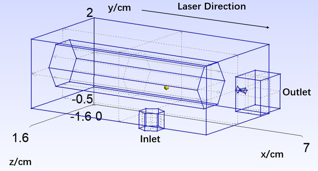
A cone with a $400\;\mu \mathrm{m}$ diameter hole serves as the aperture through which the laser enters the cell. The dimensions of the cone were selected as a compromise between achieving a higher operating density and minimizing laser-induced damage to the outlet. As shown in Figure 1, the cone is mounted on a piston that allows the aperture position to be adjusted along the laser beam axis while maintaining the gas cell seal, providing control over the target length. The cell is 5.9 cm in length with a volume of $38\kern0.22em {\mathrm{cm}}^3$ . The piston is oriented towards the laser entrance to facilitate rapid downstream access for applications such as staged acceleration.

Figure 1

A computer-aided design (CAD) rendering of the cell geometry along with a zoomed-in view of the nozzle at the laser exit.

To introduce the density down-ramp, the exit aperture is shaped into a converging–diverging nozzle, approximating de Laval nozzles that are used for accelerating fluids to supersonic speed^[ Reference Deshpande, Vidwans, Mahale, Joshi and Jagtap ^{42 ]}. The resulting longer ramps would help collimate the naturally divergent electron beams produced by LWFA. Figure 1 includes a detailed view of the converging–diverging nozzle. The converging section began with a diameter of 1.9 mm and was extended 0.8 mm in length. The throat section measured 1.0 mm in diameter and 0.1 mm in length. The diverging section extended 1.7 mm, widening to a final diameter of 1.6 mm.

Ryujin defines the initial conditions on either side of the inlet interface using two sets of primitive states. A primitive state refers to a set of physical parameters that describe the fluid at a given point, including density, thermal velocity and pressure. In this study, we simulated pure helium with an inlet pressure of 100 mbar. The density was determined using the ideal gas law, assuming a temperature of 300 K. The velocity of the primitive state corresponds to the mean thermal velocity of gas particles as derived from the Boltzmann distribution. The initial vacuum pressure was assumed to be ${10}^{-5}\ \mathrm{mbar}$ .

The Knudsen number, $\mathrm{Kn}$ , is the ratio of the molecular mean free path to the physical scale in the system. It characterizes the type of the flow. For $Kn<0.01$ , the continuum flow assumption is valid, and the no-slip boundary condition applies. For $0.01< \mathrm{Kn}<0.1$ , the velocity slip at the wall becomes important, and the slip boundary conditions should be used^[ Reference Zhang, Shan, Zhao and Guo ^{43 ]}. The Knudsen number for helium at 300 K and 100 mbar, with the nozzle throat as the smallest length scale at 0.1 mm, is approximately $0.0138$ . This value indicates that the gas flow in the cell is within the slip-flow regime and, consequently, for these simulations, the wall conditions were set to slip.

4 Simulation results

To evaluate the capability of Ryujin, we first conducted 2D trial simulations using a simplified geometry without the piston. Figure 2(a) shows transverse slices of the density distribution at 5 and 50 ms after gas release. At 5 ms, the system had not yet reached equilibrium, and a higher density was found near the inlet. By 50 ms, the density had stabilized and become uniform. As shown in Figure 2(b), the density plateaued at $4.91\times {10}^{25}\ {\mathrm{m}}^{-3}$ after 50 ms. An exponential fit to the mean density reveals a characteristic time of 16 ms.

Figure 2

Helium atomic density distribution and uniformity for the 2D cell without a piston. (a) Transverse slices of the density distribution at 5 and 50 ms. (b) Mean helium atomic density in the gas cell as a function of time after gas release. (c) Temporal evolution of density uniformity (standard deviation) in the gas cell.

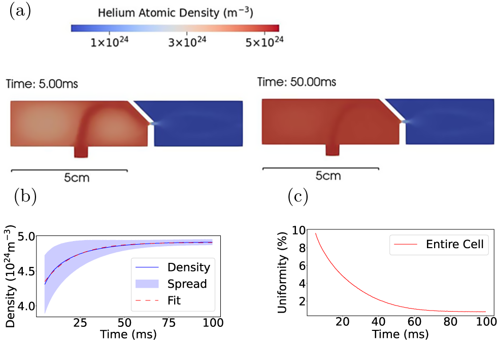
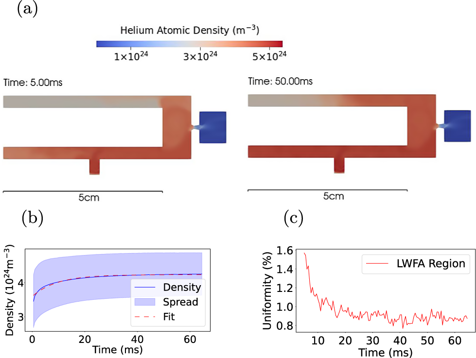
Figure 3 presents the results of the 2D simulation, including the trombone, as implemented in the variable length gas cell. The distance from the trombone to the outlet was set to 9 mm. Figure 3(a) shows transverse slices of the density distribution at 5 and 50 ms after gas release, which also illustrate the cell geometry. The cell comprised an inlet at the bottom and a piston inside. The outlet on the piston was neglected, as this area was significantly smaller compared to the nozzle size. The right-hand wall served as the outlet. At 5 ms, the flow is again quite nonuniform, but the mean density is observed to have stabilized at $4.24\times {10}^{25}\ {\mathrm{m}}^{-3}$ after 40 ms, as shown in Figure 3(b). The density evolution indicated a characteristic time of 9.3 ms. The density inhomogeneity in the LWFA region, defined as a cylindrical volume within the cell with a radius twice that of the outlet and centred along the laser direction, decreased to below $1\%$ after 15 ms, as shown in Figure 3(c). However, the density inhomogeneity across the entire cell remains above 15%, at 50 ms. As illustrated in Figure 3(a), density gradients persist in the top left-hand corner even after the mean density throughout the cell has stabilized. The complex geometry of the cell obstructs fluid flow to the corners, thereby leading to persistent nonuniformities in the density distribution. In addition, the presence of the piston results in a reduced characteristic time, attributed to the smaller effective volume compared to configurations without the piston.

Figure 3

Helium atomic density distribution and uniformity for the 2D cell geometry with a piston. (a) Transverse slices of the density distribution at 5 and 50 ms. (b) Mean helium atomic density in the gas cell as a function of time after gas release. (c) Temporal evolution of density uniformity (standard deviation) in the LWFA region.

While 2D simulations provide useful insights into general flow behaviour, they inherently lack the ability to capture the full spatial complexity of gas dynamics within the cell. Transitioning to 3D simulation is crucial for further investigation of the density equilibrium time and the density inhomogeneities caused by the cell’s geometry and outlet configuration, but the complex geometry increases the computational difficulty. The 3D finite-element mesh requires particular consideration. Currently, Ryujin only accepts quadrilateral and hexahedral mesh elements. While tetrahedral meshing offers greater flexibility for handling complex geometries, it is prone to numerical diffusion, particularly when modelling shocks and sharp density transitions^[ Reference Kotrasova and Michalcova ^{44 ]}. By contrast, the hexahedral mesh provides higher accuracy, but generating a fine mesh for complex geometries is challenging. For simplification, the cylindrical piston was replaced by a hexagonal-shaped rod inside the cell. In addition, the cones defining the converging–diverging nozzles were approximated using polygons, while squares were used to represent the outlet, reducing computational time. A 3D finite-element mesh generator, known as Gmsh^[ Reference Geuzaine and Remacle ^{45 ]}, was used to generate the Ryujin inputs. It features the ability to force the mesh elements to be hexahedral, and 3D volume meshes were created as a compromise between the mesh quality and the computation time. The simulations were performed on the Imperial HPC system with eight Icelake CPU cores^{[ 46 ]}. It took a day to compute 300 ms for the 3D simulations, compared to a few hours for the 2D simulations. The 3D mesh resolution resulted in about 35,000 collocation points, which amounted to 175,000 total spatial degrees of freedom.

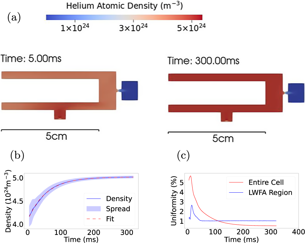
Figure 4 presents the gas cell geometry used for the 3D simulation. Figure 5(a) displays transverse slices of the density distribution at 5 and 300 ms after gas release. As observed in 2D simulations, the density within the cell becomes uniform upon reaching equilibrium. The mean density inside the cell was projected to plateau at 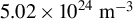$5.02\times {10}^{24}\ {\mathrm{m}}^{-3}$ , as shown in Figure 5(b). The characteristic time for the density increase was 56 ms, and the density nonuniformity within the cell decreased below $1\%$ after 100 ms, as depicted in Figure 5(c). Figure 5(c) also compares the density nonuniformity in both the entire cell and the LWFA region. The LWFA region exhibited smaller final density spread. After the initial fluctuation, the density spread plateaued at 1% beyond 40 ms.

Figure 4

Visualization of the 3D cell geometry in Gmsh.

Figure 5

Helium atomic density distribution and uniformity for the 3D cell geometry. (a) Transverse slices of the density distribution at 5 and 300 ms. (b) Mean helium atomic density in the entire cell and in the LWFA region as a function of time after gas release. (c) Temporal evolution of density uniformity (standard deviation) in the entire cell and the LWFA region.

The characteristic time scale, $\tau$ , represents the exponential time constant for density stabilization. Achieving uniformity within 1% requires approximately two to three characteristic time periods. This time determines the minimum laser delay necessary to ensure a uniform density. The characteristic time can be estimated as the ratio of the fluid mass contained within the cell to the mass flow rate exiting through the nozzle, given by the following^[ Reference Golijanek-Jedrzejczyk, Świsulski, Hanus, Zych and Petryka ^{47 ]}:

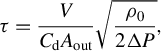(1) $$\begin{align}\tau =\frac{V}{C_\mathrm{d}{A}_\mathrm{out}}\sqrt{\frac{\rho_0}{2\Delta P}},\end{align}$$

where ${\rho}_0$ is the mass density and $\Delta P$ is the pressure difference between the cell and the vacuum. The volume of the cell and the area of the outlet are denoted by $V$ and ${A}_\mathrm{out}$ , respectively. When the inlet size is significantly larger than the outlet, the gas fills the cell on a timescale that is much shorter than the density equilibrium time. Although the initial filling dynamics of an empty gas cell are strongly governed by the inlet area, the outlet size ultimately determines the rate at which the system approaches density equilibrium. Here, ${C}_\mathrm{d}$ is the discharge coefficient, which is close to unity for a nozzle^[ Reference Woodward ^{48 ]}.

Table 1 summarizes the equilibrium times obtained from the simulations, alongside the values predicted by Equation (1), assuming the outlet size of 1 mm, equivalent to the throat size. Equation (1) accurately predicts the equilibrium time in 3D simulations, with deviations at the percent level.

Table 1

Comparison of the equilibrium time obtained from simulations ( ${\tau}_\mathrm{sim}$ ) with the theoretical value ( ${\tau}_\mathrm{theory}$ ) predicted by Equation (1), along with the percentage difference between them.

In the 2D simulations, the case with the piston exhibited a shorter equilibrium time compared to the case without the piston, as expected from theoretical predictions, due to the smaller effective cell volume. However, in the 2D case, the concept of volume becomes ambiguous. The 2D model effectively assumes the cell extends infinitely in the direction perpendicular to the simulation plane, such that the influence of the third dimension is negligible. As a result, the volume-to-outlet area ratio reduces to the ratio of the cell’s cross-sectional area to the outlet length. Equation (1) can then be reformulated as follows:

(2) $$\begin{align}{\tau}_{3\mathrm{d}}={\tau}_{2\mathrm{d}}\frac{2{L}_\mathrm{cell}}{\pi {r}_\mathrm{out}},\end{align}$$

where ${L}_\mathrm{cell}$ is the length of the cell in the direction perpendicular to the plane of the 2D simulation. Based on this relation, Figure 5(b) is expected to show a characteristic time 40 times larger than in Figure 3(b). A longer equilibrium time was observed in the 3D case as compared to the 2D case. However, the predicted time for the 2D case was almost an order of magnitude lower than the computational results. This discrepancy arises from the complex internal geometry of the gas cell, which the simplified model does not fully account for. As shown in Figure 3(b), the upper section of the gas cell is connected to the inlet only via a narrow path around the piston tip, which restricts gas flow and leads to a prolonged equilibrium time. By contrast, in the 3D case the gas flow from the inlet is less obstructed, resulting in a shorter equilibrium time that differs by only $1.5\%$ from the theoretical prediction. The 3D fluid simulation, combined with the theoretical model, provides an accurate estimation of the density equilibrium time for the gas cell target. This capability is readily extendable to arbitrary gas cell targets and even other types of LWFA targets, thereby aiding target design by providing reliable equilibrium time estimates. Owing to the convex limiting feature, Ryujin remains robust when simulating complex geometries, which broadens the applicability of Ryujin to a wide range of wakefield targets.

The cell studied here exhibits a characteristic recovery time of approximately 56 ms, with density equilibrium established between 100 and 200 ms. This corresponds to a maximum repetition rate of 5–10 Hz. The transverse cross-section of the cell is about 3 cm by 2 cm. If reduced to 1 cm by 1 cm or less, the repetition rate could increase by a factor of 6–10. The outlet area can also be increased, albeit at the cost of a shorter density ramp length. Such a cell would be well-suited for high-repetition-rate LWFA.

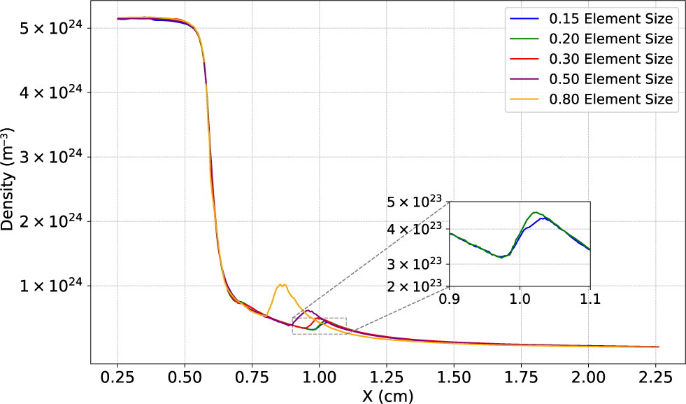
To investigate the density down-ramp, we conducted a 2D convergence study of the density profile using a reduced geometry consisting of only the outlet nozzle. Figure 6 compares the on-axis density profile along the down-ramp for different mesh resolutions, characterized by the element size factor. This factor represents the element size relative to the characteristic Gmsh size, which is heuristically determined as a fraction of the geometry’s bounding box size and further refined based on the smallest geometric features. All the simulations with varying element sizes produced the same uniform density within the gas cell and a consistent down-ramp profile for 0.25 cm $<x<$ 0.75 cm. This indicates that the mesh resolution does not significantly influence the density plateau or the ramp scale-length. However, for a coarse mesh an artificial thickness is assigned to the density bump that forms at the location where the shockwaves, generated by discontinuities in the nozzle, rejoin. The inset in Figure 6 reveals that the density profile begins to converge at an element size of 0.06. While this does not alter the gas flow within the cell, a fine mesh resolution is necessary to accurately capture the key features of the supersonic flows emerging from the nozzles. The peak density of the bump is orders of magnitude lower than the plateau density, as shown in Figure 6. Hence, this feature is not expected to significantly influence the dynamics of the wakefield accelerator.

Figure 6

Convergence scan of the density down-ramp profile using 2D simulations.

To characterize the length of the density down-ramp, an analytical function of

(3) $$\begin{align}\rho ={\rho}_0{\left({e}^{-x/\lambda }+1\right)}^{-1}\end{align}$$

was fitted to the on-axis density lineout for the fluid simulation with an element size of 0.06. Here, ${\rho}_0$ is the plateau density, while $\lambda$ represents the scale-length of the ramp. For a circular outlet, the scale-length $\lambda$ is approximately $R/2$ , where $R$ is the outlet radius. In the case of a nozzle that is a tailored nozzle with a throat radius of 0.5 mm, the ramp scale-length was found to be extended to 0.32 mm^[ Reference Backhouse ^{24 ]}. The converging–diverging nozzle geometry, combined with the large aperture size, contributes to an extended scale-length. Such extended ramps could be beneficial in reducing electron beam divergence from the LWFA^[ Reference Backhouse ^{24 ]}. However, obtaining experimental measurements of density profiles near the gas outlets are usually obscured by the metallic and opaque nozzle structure. This makes it difficult to have accurate measurements of this region where critical dynamics take place. Hence, integrating the results from these fluid simulations with PIC simulations provides a powerful approach to investigate density down-ramps and their role in generating low-divergence electron beams. This is vital for practical applications such as wakefield-based free-electron lasers^[ Reference Wang, Feng, Ke, Yu, Xu, Qi, Chen, Qin, Zhang, Fang, Liu, Jiang, Wang, Wang, Yang, Wu, Leng, Liu, Li and Xu ^{31 ]}.