


1. Introduction
1.1 Background and motivation
Going back to experimental work from the 1990s, the most prominent question concerning random
 $k$
-SAT has been to pinpoint the satisfiability threshold, defined as the largest density
$k$
-SAT has been to pinpoint the satisfiability threshold, defined as the largest density
 $m/n$
of clauses
$m/n$
of clauses
 $m$
to variables
$m$
to variables
 $n$
up to which satisfying assignments likely exist [Reference Achlioptas, Naor and Peres6, Reference Cheeseman, Kanefsky and Taylor18]. Currently, the satisfiability threshold is known precisely in the case of
$n$
up to which satisfying assignments likely exist [Reference Achlioptas, Naor and Peres6, Reference Cheeseman, Kanefsky and Taylor18]. Currently, the satisfiability threshold is known precisely in the case of
 $k=2$
[Reference Chvátal and Reed21, Reference Goerdt41] and for
$k=2$
[Reference Chvátal and Reed21, Reference Goerdt41] and for
 $k\geq k_0$
with
$k\geq k_0$
with
 $k_0$
an undetermined (large) constant [Reference Ding, Sly and Sun34]. The latter result confirms ‘predictions’ based on an analytic but non-rigorous physics technique called the ‘cavity method’. Indeed, the cavity method predicts the satisfiability threshold for every
$k_0$
an undetermined (large) constant [Reference Ding, Sly and Sun34]. The latter result confirms ‘predictions’ based on an analytic but non-rigorous physics technique called the ‘cavity method’. Indeed, the cavity method predicts the satisfiability threshold for every
 $k\geq 3$
[Reference Mézard, Parisi and Zecchina52], but random
$k\geq 3$
[Reference Mézard, Parisi and Zecchina52], but random
 $k$
-SAT for ‘small’
$k$
-SAT for ‘small’
 $k\geq 3$
appears to be a particularly hard nut to crack. Additionally, according to the cavity method several phase transitions precede the satisfiability threshold and are expected to impact, among other things, the performance of algorithms [Reference Krzakala, Montanari, Ricci-Tersenghi, Semerjian and Zdeborová48]. One of these phase transitions, the Gibbs uniqueness transition, pertains to a spatial mixing property that also plays a pivotal role in the computational complexity of counting and sampling [Reference Sly62].
$k\geq 3$
appears to be a particularly hard nut to crack. Additionally, according to the cavity method several phase transitions precede the satisfiability threshold and are expected to impact, among other things, the performance of algorithms [Reference Krzakala, Montanari, Ricci-Tersenghi, Semerjian and Zdeborová48]. One of these phase transitions, the Gibbs uniqueness transition, pertains to a spatial mixing property that also plays a pivotal role in the computational complexity of counting and sampling [Reference Sly62].
From a statistical physics viewpoint, the satisfiability threshold is only the second most important quantity associated with random
 $k$
-SAT. The first place firmly belongs to the typical number of satisfying assignments, known as the partition function in physics parlance [Reference Mézard and Montanari51]. All the other predictions, including the location of the satisfiability threshold, ultimately derive from the formula for the number of satisfying assignments or closely related variables [Reference Mertens, Mézard and Zecchina50]. Yet there has been little progress on confirming the physics formula for the number of satisfying assignments rigorously.
$k$
-SAT. The first place firmly belongs to the typical number of satisfying assignments, known as the partition function in physics parlance [Reference Mézard and Montanari51]. All the other predictions, including the location of the satisfiability threshold, ultimately derive from the formula for the number of satisfying assignments or closely related variables [Reference Mertens, Mézard and Zecchina50]. Yet there has been little progress on confirming the physics formula for the number of satisfying assignments rigorously.
Three prior contributions stand out. First, a proof technique called the ‘interpolation method’ turns the physics prediction into a rigorous upper bound [Reference Franz and Leone36, Reference Guerra42, Reference Panchenko and Talagrand61].Footnote 1 Second, in the case
 $k=2$
, conceptually much simpler than
$k=2$
, conceptually much simpler than
 $k\geq 3$
, the physics formula has been proved correct [Reference Achlioptas, Coja-Oghlan and Hahn-Klimroth3]. Third, Montanari and Shah [Reference Montanari and Shah57] proved that also for
$k\geq 3$
, the physics formula has been proved correct [Reference Achlioptas, Coja-Oghlan and Hahn-Klimroth3]. Third, Montanari and Shah [Reference Montanari and Shah57] proved that also for
 $k\geq 3$
for certain clause/variable densities the ‘replica symmetric solution’ from physics correctly approximates the number of ‘good’ assignments that satisfy all but
$k\geq 3$
for certain clause/variable densities the ‘replica symmetric solution’ from physics correctly approximates the number of ‘good’ assignments that satisfy all but
 $o(n)$
clauses. However, it seems difficult to estimate the gap between the number of such ‘good’ assignments and the number of actual satisfying assignments. A rigorous method to this effect would likely imply the existence of uniform satisfiability thresholds for all
$o(n)$
clauses. However, it seems difficult to estimate the gap between the number of such ‘good’ assignments and the number of actual satisfying assignments. A rigorous method to this effect would likely imply the existence of uniform satisfiability thresholds for all
 $k\geq 3$
, thereby resolving a long-standing conundrum [Reference Bayati, Gamarnik and Tetali12, Reference Friedgut37]. The proof of Montanari and Shah is based on the aforementioned Gibbs uniqueness property.
$k\geq 3$
, thereby resolving a long-standing conundrum [Reference Bayati, Gamarnik and Tetali12, Reference Friedgut37]. The proof of Montanari and Shah is based on the aforementioned Gibbs uniqueness property.
The aim of the present paper is to determine the number of actual satisfying assignments of random
 $k$
-SAT formulas for clause/variable densities up to the Gibbs uniqueness threshold. Specifically, we verify that the ‘replica symmetric solution’ from [Reference Monasson and Zecchina55, Reference Monasson and Zecchina56] yields the correct answer for any
$k$
-SAT formulas for clause/variable densities up to the Gibbs uniqueness threshold. Specifically, we verify that the ‘replica symmetric solution’ from [Reference Monasson and Zecchina55, Reference Monasson and Zecchina56] yields the correct answer for any
 $k\geq 3$
right up to the Gibbs uniqueness threshold, even though the precise value of this threshold is not currently known. Additionally, we derive a new lower bound on the Gibbs uniqueness threshold. The improvement is particularly significant for ‘small’
$k\geq 3$
right up to the Gibbs uniqueness threshold, even though the precise value of this threshold is not currently known. Additionally, we derive a new lower bound on the Gibbs uniqueness threshold. The improvement is particularly significant for ‘small’
 $k\geq 3$
. Combining these two results, we obtain the first rigorous formula for the number of satisfying assignments of random
$k\geq 3$
. Combining these two results, we obtain the first rigorous formula for the number of satisfying assignments of random
 $k$
-SAT formula for a non-trivial regime of clause/variable densities. Crucially, the result covers meaningful clause/variable densities even for small
$k$
-SAT formula for a non-trivial regime of clause/variable densities. Crucially, the result covers meaningful clause/variable densities even for small
 $k\geq 3$
.
$k\geq 3$
.
1.2 Results
Let
 $\boldsymbol{\Phi }=\boldsymbol{\Phi }_{d,k}(n)$
be the random
$\boldsymbol{\Phi }=\boldsymbol{\Phi }_{d,k}(n)$
be the random
 $k$
-CNF on
$k$
-CNF on
 $n$
Boolean variables
$n$
Boolean variables
 $x_1,\ldots ,x_n$
with
$x_1,\ldots ,x_n$
with
 $\boldsymbol{m}=\boldsymbol{m}_n\sim \textrm {Po}(dn/k)$
clauses
$\boldsymbol{m}=\boldsymbol{m}_n\sim \textrm {Po}(dn/k)$
clauses
 $a_1,\ldots ,a_{\boldsymbol{m}}$
. The clauses
$a_1,\ldots ,a_{\boldsymbol{m}}$
. The clauses
 $a_i$
are drawn independently and uniformly from the set of all
$a_i$
are drawn independently and uniformly from the set of all
 $2^k \binom {n}{k}$
possible clauses with
$2^k \binom {n}{k}$
possible clauses with
 $k$
distinct variables. Hence, the parameter
$k$
distinct variables. Hence, the parameter
 $d$
prescribes the expected number of clauses in which a given variable appears. Let
$d$
prescribes the expected number of clauses in which a given variable appears. Let
 $S(\boldsymbol{\Phi })$
be the set of satisfying assignments of
$S(\boldsymbol{\Phi })$
be the set of satisfying assignments of
 $\boldsymbol{\Phi }$
and let
$\boldsymbol{\Phi }$
and let
 $Z(\boldsymbol{\Phi })=|S(\boldsymbol{\Phi })|$
. We encode the Boolean values ‘true’ and ‘false’ by
$Z(\boldsymbol{\Phi })=|S(\boldsymbol{\Phi })|$
. We encode the Boolean values ‘true’ and ‘false’ by
 $+1$
and
$+1$
and
 $-1$
, respectively. Since right up to the satisfiability threshold
$-1$
, respectively. Since right up to the satisfiability threshold
 $Z(\boldsymbol{\Phi })$
is of order
$Z(\boldsymbol{\Phi })$
is of order
 $\exp (\Theta (n))$
w.h.p. for trivial reasons,Footnote 2 our objective is to study the random variable
$\exp (\Theta (n))$
w.h.p. for trivial reasons,Footnote 2 our objective is to study the random variable
 $n^{-1}\log Z(\boldsymbol{\Phi })$
as
$n^{-1}\log Z(\boldsymbol{\Phi })$
as
 $n\to \infty$
.
$n\to \infty$
.
1.2.1 The number of satisfying assignments up to the Gibbs uniqueness threshold
The first main result vindicates the ‘replica symmetric solution’ for values of
 $d$
up to the Gibbs uniqueness threshold of the Galton-Watson tree that mimics the local topology of
$d$
up to the Gibbs uniqueness threshold of the Galton-Watson tree that mimics the local topology of
 $\boldsymbol{\Phi }$
. Let us define these concepts precisely.
$\boldsymbol{\Phi }$
. Let us define these concepts precisely.
We begin with the Galton-Watson tree
 $\mathbb{T}=\mathbb{T}_{d,k}$
, which is generated by a two-type branching process. The two types are variable nodes and clause nodes. The process starts with a single root variable node
$\mathbb{T}=\mathbb{T}_{d,k}$
, which is generated by a two-type branching process. The two types are variable nodes and clause nodes. The process starts with a single root variable node
 $\mathfrak{x}$
. The offspring of any variable node is a
$\mathfrak{x}$
. The offspring of any variable node is a
 $\textrm {Po}(d)$
number of clause nodes, while every clause node begets precisely
$\textrm {Po}(d)$
number of clause nodes, while every clause node begets precisely
 $k-1$
variable nodes. Additionally, independently for each clause node
$k-1$
variable nodes. Additionally, independently for each clause node
 $a$
and every variable node
$a$
and every variable node
 $x$
that is either a child or the parent of
$x$
that is either a child or the parent of
 $a$
a sign, denoted
$a$
a sign, denoted
 $\mathrm{sign}(x,a)\in \{\pm 1\}$
, is chosen uniformly at random. The resulting random tree
$\mathrm{sign}(x,a)\in \{\pm 1\}$
, is chosen uniformly at random. The resulting random tree
 $\mathbb{T}$
models the local structure of the random formula
$\mathbb{T}$
models the local structure of the random formula
 $\boldsymbol{\Phi }$
in the sense of local weak convergence [Reference Aldous, Steele and Kesten9, Reference Lovász49].Footnote 3
$\boldsymbol{\Phi }$
in the sense of local weak convergence [Reference Aldous, Steele and Kesten9, Reference Lovász49].Footnote 3
Next, we define the Gibbs uniqueness property on the tree
 $\mathbb{T}$
. For an integer
$\mathbb{T}$
. For an integer
 $\ell \geq 0$
let
$\ell \geq 0$
let
 $\mathbb{T}^{(\ell )}$
be the finite tree obtained by removing all variable and clause nodes at a distance greater than
$\mathbb{T}^{(\ell )}$
be the finite tree obtained by removing all variable and clause nodes at a distance greater than
 $2\ell$
from the root
$2\ell$
from the root
 $\mathfrak{x}$
. We identify the finite tree
$\mathfrak{x}$
. We identify the finite tree
 $\mathbb{T}^{(\ell )}$
with a Boolean formula whose variables/clauses are precisely the variable/clause nodes of
$\mathbb{T}^{(\ell )}$
with a Boolean formula whose variables/clauses are precisely the variable/clause nodes of
 $\mathbb{T}^{(\ell )}$
. Let
$\mathbb{T}^{(\ell )}$
. Let
 $S(\mathbb{T}^{(\ell )})\neq \emptyset$
be the set of satisfying assignments of this formula and let
$S(\mathbb{T}^{(\ell )})\neq \emptyset$
be the set of satisfying assignments of this formula and let
 $\boldsymbol{\tau }^{(\ell )}\in S(\mathbb{T}^{(\ell )})$
be a uniformly random satisfying assignment. Moreover, let
$\boldsymbol{\tau }^{(\ell )}\in S(\mathbb{T}^{(\ell )})$
be a uniformly random satisfying assignment. Moreover, let
 $\partial ^{2\ell }\mathfrak{x}$
be the set of variable nodes of
$\partial ^{2\ell }\mathfrak{x}$
be the set of variable nodes of
 $\mathbb{T}^{(\ell )}$
at distance precisely
$\mathbb{T}^{(\ell )}$
at distance precisely
 $2\ell$
from the root
$2\ell$
from the root
 $\mathfrak{x}$
. Then for given
$\mathfrak{x}$
. Then for given
 $d,k$
the tree
$d,k$
the tree
 $\mathbb{T}=\mathbb{T}_{d,k}$
has the Gibbs uniqueness property if
$\mathbb{T}=\mathbb{T}_{d,k}$
has the Gibbs uniqueness property if
 \begin{align} \lim _{\ell \to \infty }{\mathbb E}\bigg [ {\max _{\tau \in S(\mathbb{T}^{(\ell )})}{\kern-2pt}\left |{ {\mathbb P}\big [{\kern-1pt} {\boldsymbol{\tau }^{(\ell )}(\mathfrak{x}) = 1{\kern-1pt}\mid{\kern-.5pt} \mathbb{T}}\big ] {-}{\mathbb P}\big [ {\boldsymbol{\tau }^{(\ell )}(\mathfrak{x}) = 1{\kern-1pt}\mid{\kern-.5pt} \mathbb{T},\,\forall x\in \partial ^{2\ell }\mathfrak{x}\,:\,\boldsymbol{\tau }^{(\ell )}(x)=\tau (x)}\big ] }\right |}{\kern-1pt}\bigg ]{\kern-1pt} & =0 & & {\kern-2pt}\mbox{(see [47])}. \end{align}
In words, in the limit of large
 $\ell$
the truth value
$\ell$
the truth value
 $\boldsymbol{\tau }^{(\ell )}(\mathfrak{x})$
of the root
$\boldsymbol{\tau }^{(\ell )}(\mathfrak{x})$
of the root
 $\mathfrak{x}$
is asymptotically independent of the truth values
$\mathfrak{x}$
is asymptotically independent of the truth values
 $\{\boldsymbol{\tau }^{(\ell )}(x)\}_{x\in \partial ^{2\ell }\mathfrak{x}}$
of the variables at distance
$\{\boldsymbol{\tau }^{(\ell )}(x)\}_{x\in \partial ^{2\ell }\mathfrak{x}}$
of the variables at distance
 $2\ell$
from
$2\ell$
from
 $\mathfrak{x}$
. In light of the above, for any
$\mathfrak{x}$
. In light of the above, for any
 $k \ge 2$
we further define
$k \ge 2$
we further define
 $d_{\mathrm{uniq}}(k)$
as
$d_{\mathrm{uniq}}(k)$
as
 \begin{align} d_{\mathrm{uniq}}(k) = \inf \{ d\gt 0\,: \text{ condition (1.1) fails to hold for } {d,k}\}. \end{align}
It is easy to see that
 $d_{\mathrm{uniq}}(k)$
is strictly positive and finite for any
$d_{\mathrm{uniq}}(k)$
is strictly positive and finite for any
 $k\geq 2$
. Indeed, in Theorem 1.2 we will derive explicit lower bounds on
$k\geq 2$
. Indeed, in Theorem 1.2 we will derive explicit lower bounds on
 $d_{\mathrm{uniq}}(k)$
. However, the exact value of
$d_{\mathrm{uniq}}(k)$
. However, the exact value of
 $d_{\mathrm{uniq}}(k)$
is not currently known for any
$d_{\mathrm{uniq}}(k)$
is not currently known for any
 $k\geq 3$
.
$k\geq 3$
.
As a final preparation we need to spell out the ‘replica symmetric solution’ from [Reference Monasson and Zecchina55]. This prediction comes in terms of a distributional fixed point problem, i.e., a fixed point problem on the space
 $\mathscr{P}(0,1)$
of probability measures on the open unit interval. Specifically, consider the Belief Propagation operator
$\mathscr{P}(0,1)$
of probability measures on the open unit interval. Specifically, consider the Belief Propagation operator
 \begin{align} \mathrm{BP}_{d,k} & \,:\,\mathscr{P}(0,1)\to \mathscr{P}(0,1), \quad \pi \mapsto \hat {\pi }=\mathrm{BP}_{d,k}(\pi ) \end{align}
defined as follows. Let
 $\boldsymbol{d}^+,\boldsymbol{d}^-\sim \textrm {Po}(d/2)$
be Poisson variables with expectation
$\boldsymbol{d}^+,\boldsymbol{d}^-\sim \textrm {Po}(d/2)$
be Poisson variables with expectation
 $d/2$
. Moreover, let
$d/2$
. Moreover, let
 $(\boldsymbol{\mu }_{\pi ,i,j})_{i,j\geq 1}$
be a sequence of i.i.d. random variables, each following distribution
$(\boldsymbol{\mu }_{\pi ,i,j})_{i,j\geq 1}$
be a sequence of i.i.d. random variables, each following distribution
 $\pi$
. All these random variables are mutually independent. Further, let
$\pi$
. All these random variables are mutually independent. Further, let
 \begin{align} \boldsymbol{\mu }_{\pi ,i}=1-\prod _{j=1}^{k-1}\boldsymbol{\mu }_{\pi ,i,j}\quad \mbox{ for $i\geq 1$,}\quad\mbox{and}\quad \hat {\boldsymbol{\mu }}_{\pi }=\frac {\prod _{i=1}^{\boldsymbol{d}^-}\boldsymbol{\mu }_{\pi ,2i-1}}{\prod _{i=1}^{\boldsymbol{d}^-}\boldsymbol{\mu }_{\pi ,2i-1}+\prod _{i=1}^{\boldsymbol{d}^+}\boldsymbol{\mu }_{\pi ,2i}}. \end{align}
Then
 $\hat {\pi }$
is the distribution of
$\hat {\pi }$
is the distribution of
 $\hat {\boldsymbol{\mu }}_{\pi }$
. Furthermore, for a probability measure
$\hat {\boldsymbol{\mu }}_{\pi }$
. Furthermore, for a probability measure
 $\pi \in \mathscr{P}(0,1)$
define the Bethe free entropy
Footnote 4
$\pi \in \mathscr{P}(0,1)$
define the Bethe free entropy
Footnote 4
 \begin{align} \mathfrak B_{d,k}(\pi ) & ={\mathbb E}\left [ {\log \left ({\prod _{i=1}^{\boldsymbol{d}^-}\boldsymbol{\mu }_{\pi ,2i-1}+\prod _{i=1}^{\boldsymbol{d}^+}\boldsymbol{\mu }_{\pi ,2i}}\right )-\frac {d(k-1)}{k}\log \left ({1-\prod _{j=1}^k\boldsymbol{\mu }_{\pi ,1,j}}\right )}\right ] , \end{align}
provided that the expectation on the r.h.s. exists. Finally, let
 $\delta _{1/2}\in \mathscr{P}(0,1)$
be the atom at
$\delta _{1/2}\in \mathscr{P}(0,1)$
be the atom at
 $1/2$
and let us write
$1/2$
and let us write
 $\mathrm{BP}_{d,k}^\ell$
for the
$\mathrm{BP}_{d,k}^\ell$
for the
 $\ell$
-fold application of the operator
$\ell$
-fold application of the operator
 $\mathrm{BP}_{d,k}$
.
$\mathrm{BP}_{d,k}$
.
Theorem 1.1.
Let
 $k\geq 3$
and assume that
$k\geq 3$
and assume that
 $0\lt d\lt d_{\mathrm{uniq}}(k)$
. Then the weak limit
$0\lt d\lt d_{\mathrm{uniq}}(k)$
. Then the weak limit
 \begin{align} \pi _{d,k}=\lim _{\ell \to \infty }\mathrm{BP}_{d,k}^{\ell }(\delta _{1/2})\in \mathscr{P}(0,1) \end{align}
exists and
 \begin{align} \lim _{n\to \infty }\frac 1n\log Z(\boldsymbol{\Phi }) & =\mathfrak B_{d,k}(\pi _{d,k})\ \mbox{in probability}. \end{align}
The formula (1.7) matches the prediction from [Reference Monasson and Zecchina55] precisely. Of course, part of the assertion of Theorem 1.1 is that the Bethe free entropy
 $\mathfrak B_{d,k}(\pi _{d,k})$
is well defined. Admittedly, the formula (1.7) is not ‘explicit’. But the proof of Theorem 1.1 evinces that the convergence (1.6) occurs rapidly. Therefore, a randomised algorithm called ‘population dynamics’ [Reference Mézard and Montanari51] can be used to approximate (1.7) within any desired numerical accuracy.
$\mathfrak B_{d,k}(\pi _{d,k})$
is well defined. Admittedly, the formula (1.7) is not ‘explicit’. But the proof of Theorem 1.1 evinces that the convergence (1.6) occurs rapidly. Therefore, a randomised algorithm called ‘population dynamics’ [Reference Mézard and Montanari51] can be used to approximate (1.7) within any desired numerical accuracy.
1.2.2 An improved lower bound on Gibbs uniqueness
The obvious next task is to determine the Gibbs uniqueness threshold
 $d_{\mathrm{uniq}}(k)$
. Currently, its value is known precisely only in the case
$d_{\mathrm{uniq}}(k)$
. Currently, its value is known precisely only in the case
 $k=2$
, where
$k=2$
, where
 $d_{\mathrm{uniq}}(2)=2$
coincides with the random 2-SAT satisfiability threshold [Reference Achlioptas, Coja-Oghlan and Hahn-Klimroth3, Reference Chvátal and Reed21, Reference Goerdt41]. Furthermore, Montanari and Shah [Reference Montanari and Shah57] proved that the pure literal threshold
Footnote 5
$d_{\mathrm{uniq}}(2)=2$
coincides with the random 2-SAT satisfiability threshold [Reference Achlioptas, Coja-Oghlan and Hahn-Klimroth3, Reference Chvátal and Reed21, Reference Goerdt41]. Furthermore, Montanari and Shah [Reference Montanari and Shah57] proved that the pure literal threshold
Footnote 5
 $d_{\mathrm{pure}}(k)$
upper bounds
$d_{\mathrm{pure}}(k)$
upper bounds
 $d_{\mathrm{uniq}}(k)$
for all
$d_{\mathrm{uniq}}(k)$
for all
 $k\geq 2$
.Footnote 6 The value of
$k\geq 2$
.Footnote 6 The value of
 $d_{\mathrm{pure}}(k)$
admits a neat formula [Reference Broder, Frieze and Upfal16, Reference Molloy54]:
$d_{\mathrm{pure}}(k)$
admits a neat formula [Reference Broder, Frieze and Upfal16, Reference Molloy54]:
 \begin{align} d_{\mathrm{uniq}}(k)\leq d_{\mathrm{pure}}(k) & =\min _{z\gt0}\frac {z}{(1-\exp (-z/2))^{k-1}}. \end{align}
Complementing the upper bound (1.8), Montanari and Shah derived a lower bound
 $d_{\mathrm{MS}}(k)$
:
$d_{\mathrm{MS}}(k)$
:
 \begin{align} d_{\mathrm{MS}}(k) & =\sup \big \{{d\gt 0\,:\, d(k-1) ({1-\exp (-d/2)/4} ) ({1-\exp (-d/2)/2} )^{k-2} \lt 1}\big \}\leq d_{\mathrm{uniq}}(k). \end{align}
Unfortunately, the bound (1.9) is tight not even in the case
 $k=2$
, where
$k=2$
, where
 $d_{\mathrm{uniq}}(2)=2$
while
$d_{\mathrm{uniq}}(2)=2$
while
 $d_{\mathrm{MS}}(2)\approx 1.16$
. That said, the lower and upper bounds
$d_{\mathrm{MS}}(2)\approx 1.16$
. That said, the lower and upper bounds
 $d_{\mathrm{MS}}(k)$
and
$d_{\mathrm{MS}}(k)$
and
 $d_{\mathrm{pure}}(k)$
match asymptotically in the limit of large
$d_{\mathrm{pure}}(k)$
match asymptotically in the limit of large
 $k$
, as
$k$
, as
 \begin{align} d_{\mathrm{MS}}(k),d_{\mathrm{pure}}(k) & =(2+o_k(1))\log k, \end{align}
with
 $o_k(1)$
hiding a term that vanishes as
$o_k(1)$
hiding a term that vanishes as
 $k\to \infty$
. The following theorem yields an improved lower bound
$k\to \infty$
. The following theorem yields an improved lower bound
 ${{{d_{\mathrm{con}}}}}(k)$
on
${{{d_{\mathrm{con}}}}}(k)$
on
 $d_{\mathrm{uniq}}(k)$
.
$d_{\mathrm{uniq}}(k)$
.
Theorem 1.2.
For all
 $k\geq 3$
we have
$k\geq 3$
we have
 \begin{align} d_{\mathrm{uniq}}(k)\geq {{{d_{\mathrm{con}}}}}(k)\,:\!=\,\sup \left \{{d\gt 0\,:\,\frac {d(k-1)}2({1-\exp \!({-}d/2)/2})^{k-2}\lt 1}\right \}. \end{align}
An easy calculation reveals that
 \begin{align} d_{\mathrm{MS}}(k)\lt {{{d_{\mathrm{con}}}}}(k) \quad \mbox{for every }k\geq 2. \end{align}
Moreover, it is satisfactory that the formula (1.11) reproduces the correct (previously known) threshold
 $d_{\mathrm{uniq}}(2)={{{d_{\mathrm{con}}}}}(2)=d_{\mathrm{pure}}(2)=2$
. That said, we have no reason to believe that (1.11) is tight for any
$d_{\mathrm{uniq}}(2)={{{d_{\mathrm{con}}}}}(2)=d_{\mathrm{pure}}(2)=2$
. That said, we have no reason to believe that (1.11) is tight for any
 $k\geq 3$
.
$k\geq 3$
.
Combining Theorems 1.1 and 1.2, we obtain the following.
Corollary 1.3.
Let
 $k\geq 3$
. If
$k\geq 3$
. If
 $d\lt {{{d_{\mathrm{con}}}}}(k)$
then (1.7) holds.
$d\lt {{{d_{\mathrm{con}}}}}(k)$
then (1.7) holds.
Corollary 1.3 constitutes the first rigorous result to determine the precise asymptotic value of
 $\log Z(\boldsymbol{\Phi })$
for a non-trivial regime of
$\log Z(\boldsymbol{\Phi })$
for a non-trivial regime of
 $d$
for any
$d$
for any
 $k\geq 3$
. To elaborate, the formula (1.7) is trivially true for
$k\geq 3$
. To elaborate, the formula (1.7) is trivially true for
 $d\lt1/(k-1)$
because for such
$d\lt1/(k-1)$
because for such
 $d$
the
$d$
the
 $k$
-uniform hypergraph induced by the clauses of
$k$
-uniform hypergraph induced by the clauses of
 $\boldsymbol{\Phi }$
has no giant component and Belief Propagation is exact on acyclic graphical models [Reference Mézard and Montanari51]. But Corollary 1.3 applies to
$\boldsymbol{\Phi }$
has no giant component and Belief Propagation is exact on acyclic graphical models [Reference Mézard and Montanari51]. But Corollary 1.3 applies to
 $d$
well beyond this threshold, as displayed in Table 1. In particular, in contrast to much of the prior work on random
$d$
well beyond this threshold, as displayed in Table 1. In particular, in contrast to much of the prior work on random
 $k$
-SAT, Corollary 1.3 applies to a non-trivial regime of
$k$
-SAT, Corollary 1.3 applies to a non-trivial regime of
 $d$
even for ‘small’
$d$
even for ‘small’
 $k\geq 3$
.
$k\geq 3$
.
The values of
 $d_{\mathrm{MS}}(k), {{{d_{\mathrm{con}}}}}(k)$
, and
$d_{\mathrm{MS}}(k), {{{d_{\mathrm{con}}}}}(k)$
, and
 $d_{\mathrm{pure}}(k)$
for
$d_{\mathrm{pure}}(k)$
for
 $2\leq k\leq 5$
. Additionally,
$2\leq k\leq 5$
. Additionally,
 $d_{\mathrm{giant}}(k) = 1/(k-1)$
marks the giant component threshold of the hypergraph induced by the random
$d_{\mathrm{giant}}(k) = 1/(k-1)$
marks the giant component threshold of the hypergraph induced by the random
 $k$
-CNF formula. Moreover,
$k$
-CNF formula. Moreover,
 $d_{\mathrm{sat}}(k)$
is the satisfiability threshold according to physics predictions [Reference Mertens, Mézard and Zecchina50]. It is not hard to show that
$d_{\mathrm{sat}}(k)$
is the satisfiability threshold according to physics predictions [Reference Mertens, Mézard and Zecchina50]. It is not hard to show that
 $d_{\mathrm{giant}}(k) \le d_{\mathrm{MS}}(k) \le {{{d_{\mathrm{con}}}}}(k) \le d_{\mathrm{uniq}}(k) \le d_{\mathrm{pure}}(k) \le d_{\mathrm{sat}}(k)$
, for all
$d_{\mathrm{giant}}(k) \le d_{\mathrm{MS}}(k) \le {{{d_{\mathrm{con}}}}}(k) \le d_{\mathrm{uniq}}(k) \le d_{\mathrm{pure}}(k) \le d_{\mathrm{sat}}(k)$
, for all
 $k \ge 2$

Although Table 1 contains the values
 $d_{\mathrm{MS}}(k)$
from [Reference Montanari and Shah57] for comparison, we emphasise that Montanari and Shah’s result only yields the number of ‘good’ assignments satisfying all but
$d_{\mathrm{MS}}(k)$
from [Reference Montanari and Shah57] for comparison, we emphasise that Montanari and Shah’s result only yields the number of ‘good’ assignments satisfying all but
 $o(n)$
clauses, rather than of actual satisfying assignments. In fact, the best prior rigorous bounds on the number of satisfying assignments for
$o(n)$
clauses, rather than of actual satisfying assignments. In fact, the best prior rigorous bounds on the number of satisfying assignments for
 $d\gt 1/(k-1)$
derive from the first and the second moment methods. Specifically, the folklore first moment bound reads
$d\gt 1/(k-1)$
derive from the first and the second moment methods. Specifically, the folklore first moment bound reads
 \begin{align} \frac 1n\log Z(\boldsymbol{\Phi }) & \leq \log 2+\frac dk\log (1-2^{-k})+o(1)\quad \mbox{w.h.p.} \end{align}
Furthermore, Achlioptas and Peres [Reference Achlioptas and Peres7] perform a second moment argument on the number of balanced satisfying assignments, i.e., satisfying assignments that enjoy a peculiar additional condition required to keep the second moment under control. They show that w.h.p.
 \begin{align} \frac 1n & \log Z(\boldsymbol{\Phi })\geq (1-d)\log 2+\frac dk\log \left [ {\left ({\lambda ^{1/2}+\lambda ^{-1/2}}\right )^k-\lambda ^{-k/2}}\right ] +o(1),\quad \mbox{where}\\ & (1-\lambda )(1+\lambda )^{k-1}=1,\,\lambda \gt 0. \nonumber\end{align}
Figure 1 illustrates the bounds (1.13)–(1.14) along with (1.7) for
 $k=3$
. As the figure shows, the correct value (1.7) is quite close to the first moment bound. That said, the first moment bound strictly exceeds
$k=3$
. As the figure shows, the correct value (1.7) is quite close to the first moment bound. That said, the first moment bound strictly exceeds
 $\mathfrak B_{d,k}(\pi _{d,k})$
for all
$\mathfrak B_{d,k}(\pi _{d,k})$
for all
 $d\gt 0$
,
$d\gt 0$
,
 $k\geq 3$
[Reference Coja-Oghlan, Kapetanopoulos and Müller24]. On the other hand, Figure 1 demonstrates that the ‘balanced second moment bound’ (1.14) significantly undershoots
$k\geq 3$
[Reference Coja-Oghlan, Kapetanopoulos and Müller24]. On the other hand, Figure 1 demonstrates that the ‘balanced second moment bound’ (1.14) significantly undershoots
 $\mathfrak B_{d,3}(\pi _{d,3})$
. Recall that Figure 1 is on a logarithmic scale; thus, even small differences translate into exponentially large errors.
$\mathfrak B_{d,3}(\pi _{d,3})$
. Recall that Figure 1 is on a logarithmic scale; thus, even small differences translate into exponentially large errors.
Comparison of
 $\mathfrak B_{d,k}(\pi _{d,k})$
with known bounds for
$\mathfrak B_{d,k}(\pi _{d,k})$
with known bounds for
 $\lim _{n\to \infty }\frac 1n\log Z(\boldsymbol{\Phi })$
for
$\lim _{n\to \infty }\frac 1n\log Z(\boldsymbol{\Phi })$
for
 $k=3$
. The red dotted line depicts the first moment upper bound (1.13), while the green dotted line represents the lower bound provided by (1.14). The blue line displays a numerical approximation of
$k=3$
. The red dotted line depicts the first moment upper bound (1.13), while the green dotted line represents the lower bound provided by (1.14). The blue line displays a numerical approximation of
 $\mathfrak B_{d,3}(\pi _{d,3})$
. To obtain our values, we generated
$\mathfrak B_{d,3}(\pi _{d,3})$
. To obtain our values, we generated
 $10^{6}$
samples from
$10^{6}$
samples from
 $\pi \approx \mathrm{BP}^{25}_{d,3}(\delta _{1/2})$
and then evaluated the corresponding empirical average of the expression in (1.5).
$\pi \approx \mathrm{BP}^{25}_{d,3}(\delta _{1/2})$
and then evaluated the corresponding empirical average of the expression in (1.5).

1.3 Preliminaries and notation
Let
 $\Phi$
be a Boolean expression in conjunctive normal such that no clause contains the same variable twice. We write
$\Phi$
be a Boolean expression in conjunctive normal such that no clause contains the same variable twice. We write
 $V(\Phi )$
for the set of Boolean variables of
$V(\Phi )$
for the set of Boolean variables of
 $\Phi$
and
$\Phi$
and
 $F(\Phi )$
for the set of clauses. The formula
$F(\Phi )$
for the set of clauses. The formula
 $\Phi$
gives rise to a bipartite graph
$\Phi$
gives rise to a bipartite graph
 $G(\Phi )$
on the vertex set
$G(\Phi )$
on the vertex set
 $V(\Phi )\cup F(\Phi )$
in which a variable
$V(\Phi )\cup F(\Phi )$
in which a variable
 $x$
and a clause
$x$
and a clause
 $a$
are adjacent iff variable
$a$
are adjacent iff variable
 $x$
appears in clause
$x$
appears in clause
 $a$
(either positively or negatively). Let
$a$
(either positively or negatively). Let
 $E(\Phi )$
denote the edge set of the graph
$E(\Phi )$
denote the edge set of the graph
 $G(\Phi )$
. Furthermore, for a vertex
$G(\Phi )$
. Furthermore, for a vertex
 $v\in V(\Phi )\cup F(\Phi )$
let
$v\in V(\Phi )\cup F(\Phi )$
let
 $\partial _\Phi v$
be the set of neighbours of
$\partial _\Phi v$
be the set of neighbours of
 $v$
; where the reference to
$v$
; where the reference to
 $\Phi$
is self-evident, we just write
$\Phi$
is self-evident, we just write
 $\partial v$
.
$\partial v$
.
The graph
 $G(\Phi )$
induces a metric on
$G(\Phi )$
induces a metric on
 $V(\Phi )\cup F(\Phi )$
by letting
$V(\Phi )\cup F(\Phi )$
by letting
 $\mathrm{dist}_\Phi (v,w)$
equal the length of the shortest path from
$\mathrm{dist}_\Phi (v,w)$
equal the length of the shortest path from
 $v$
to
$v$
to
 $w$
. For a vertex
$w$
. For a vertex
 $v$
and an integer
$v$
and an integer
 $\ell \geq 0$
let
$\ell \geq 0$
let
 $\partial ^\ell _\Phi v=\partial ^\ell v$
be the set of all vertices
$\partial ^\ell _\Phi v=\partial ^\ell v$
be the set of all vertices
 $w$
at distance precisely
$w$
at distance precisely
 $\ell$
from
$\ell$
from
 $v$
.
$v$
.
For a clause
 $a$
and a variable
$a$
and a variable
 $x\in \partial a$
we define
$x\in \partial a$
we define
 $\mathrm{sign}_\Phi (x,a)=1$
if
$\mathrm{sign}_\Phi (x,a)=1$
if
 $a$
contains
$a$
contains
 $x$
as a positive literal, and
$x$
as a positive literal, and
 $\mathrm{sign}_\Phi (x,a)=-1$
if
$\mathrm{sign}_\Phi (x,a)=-1$
if
 $a$
contains the negation
$a$
contains the negation
 $\neg x$
. (This is unambiguous because clause
$\neg x$
. (This is unambiguous because clause
 $a$
is not allowed to contain both
$a$
is not allowed to contain both
 $x$
and
$x$
and
 $\neg x$
.) For a variable
$\neg x$
.) For a variable
 $x\in V(\Phi )$
and
$x\in V(\Phi )$
and
 $s\in \{\pm 1\}$
we let
$s\in \{\pm 1\}$
we let
 $\partial ^s_\Phi x=\partial ^sx$
be the set of clauses
$\partial ^s_\Phi x=\partial ^sx$
be the set of clauses
 $a\in \partial _\Phi x$
such that
$a\in \partial _\Phi x$
such that
 $\mathrm{sign}_\Phi (x,a)=s$
. Where convenient we use the shorthand
$\mathrm{sign}_\Phi (x,a)=s$
. Where convenient we use the shorthand
 $\partial ^\pm x=\partial ^{\pm 1}x$
. We say that a variable
$\partial ^\pm x=\partial ^{\pm 1}x$
. We say that a variable
 $x$
is pure in
$x$
is pure in
 $\Phi$
if
$\Phi$
if
 $\mathrm{sign}_\Phi (x,a)=\mathrm{sign}_\Phi (x,b)$
for all
$\mathrm{sign}_\Phi (x,a)=\mathrm{sign}_\Phi (x,b)$
for all
 $a,b\in \partial x$
. More specifically, say that
$a,b\in \partial x$
. More specifically, say that
 $x$
is a pure literal of
$x$
is a pure literal of
 $\Phi$
if
$\Phi$
if
 $\partial ^-x=\emptyset$
. Similarly,
$\partial ^-x=\emptyset$
. Similarly,
 $\neg x$
is called a pure literal if
$\neg x$
is called a pure literal if
 $\partial ^+x=\emptyset$
. A variable or literal that fails to be pure is called mixed.
$\partial ^+x=\emptyset$
. A variable or literal that fails to be pure is called mixed.
For a literal
 $l\in \{x,\neg x\,:\,x\in V(\Phi )\}$
we let
$l\in \{x,\neg x\,:\,x\in V(\Phi )\}$
we let
 $|l|$
denote the underlying variable; thus,
$|l|$
denote the underlying variable; thus,
 $|x|=|\neg x|=x$
for
$|x|=|\neg x|=x$
for
 $x\in V(\Phi )$
. Moreover, we define
$x\in V(\Phi )$
. Moreover, we define
 $\mathrm{sign}(x)=1$
and
$\mathrm{sign}(x)=1$
and
 $\mathrm{sign}(\neg x)=-1$
. Further, for a literal
$\mathrm{sign}(\neg x)=-1$
. Further, for a literal
 $l$
we define
$l$
we define
 $1\cdot l=l$
and
$1\cdot l=l$
and
 $(-1)\cdot l=\neg l$
.
$(-1)\cdot l=\neg l$
.
If
 $\Phi$
is satisfiable, then
$\Phi$
is satisfiable, then
 $\boldsymbol{\sigma }_\Phi =(\boldsymbol{\sigma }_\Phi (x))_{x\in V(\Phi )}$
denotes a uniformly random satisfying assignment of
$\boldsymbol{\sigma }_\Phi =(\boldsymbol{\sigma }_\Phi (x))_{x\in V(\Phi )}$
denotes a uniformly random satisfying assignment of
 $\Phi$
. Where the reference to
$\Phi$
. Where the reference to
 $\Phi$
is obvious we just write
$\Phi$
is obvious we just write
 $\boldsymbol{\sigma }$
.
$\boldsymbol{\sigma }$
.
Let
 $\mu ,\nu$
be two probability measures on
$\mu ,\nu$
be two probability measures on
 $\mathbb{R}^h$
, let
$\mathbb{R}^h$
, let
 $q\geq 1$
and assume that
$q\geq 1$
and assume that
 $\int _{\mathbb{R}^h}\|x\|_q^q{\mathrm d}\mu (x),\int _{\mathbb{R}^h}\|x\|_q^q{\mathrm d}\nu (x)\lt \infty$
. We recall that the
$\int _{\mathbb{R}^h}\|x\|_q^q{\mathrm d}\mu (x),\int _{\mathbb{R}^h}\|x\|_q^q{\mathrm d}\nu (x)\lt \infty$
. We recall that the
 $L_q$
-Wasserstein distance of
$L_q$
-Wasserstein distance of
 $\mu ,\nu$
is defined as
$\mu ,\nu$
is defined as
 \begin{align*} W_q(\mu,\nu ) & =\inf _{(\boldsymbol{\xi },\boldsymbol{\zeta })}{\mathbb E}\left [ {\|\boldsymbol{\xi }-\boldsymbol{\zeta }\|_q^q}\right ] ^{1/q}, \end{align*}
where the infimum is taken over all pairs
 $(\boldsymbol{\xi },\boldsymbol{\zeta })$
of random variables defined on the same probability space
$(\boldsymbol{\xi },\boldsymbol{\zeta })$
of random variables defined on the same probability space
 $\Omega$
such that
$\Omega$
such that
 $\boldsymbol{\xi }$
has distribution
$\boldsymbol{\xi }$
has distribution
 $\mu$
and
$\mu$
and
 $\boldsymbol{\zeta }$
has distribution
$\boldsymbol{\zeta }$
has distribution
 $\nu$
. If
$\nu$
. If
 $\boldsymbol{X},\boldsymbol{Y}$
are random variables with distributions
$\boldsymbol{X},\boldsymbol{Y}$
are random variables with distributions
 $\mu ,\nu$
, it is convenient to use the shorthand
$\mu ,\nu$
, it is convenient to use the shorthand
 $W_q(\boldsymbol{X},\boldsymbol{Y})=W_q(\mu ,\nu )$
, provided that
$W_q(\boldsymbol{X},\boldsymbol{Y})=W_q(\mu ,\nu )$
, provided that
 ${\mathbb E}[\|\boldsymbol{X}\|_q^q],{\mathbb E}[\|\boldsymbol{Y}\|_q^q]\lt \infty$
.
${\mathbb E}[\|\boldsymbol{X}\|_q^q],{\mathbb E}[\|\boldsymbol{Y}\|_q^q]\lt \infty$
.
For two random variables
 $\boldsymbol{X},\boldsymbol{Y}$
we write
$\boldsymbol{X},\boldsymbol{Y}$
we write
 $\boldsymbol{X}\sim \boldsymbol{Y}$
if
$\boldsymbol{X}\sim \boldsymbol{Y}$
if
 $\boldsymbol{X},\boldsymbol{Y}$
are identically distributed. Moreover, for a probability distribution
$\boldsymbol{X},\boldsymbol{Y}$
are identically distributed. Moreover, for a probability distribution
 $\mu$
and a random variable
$\mu$
and a random variable
 $\boldsymbol{X}$
we write
$\boldsymbol{X}$
we write
 $\boldsymbol{X}\sim \mu$
if
$\boldsymbol{X}\sim \mu$
if
 $\boldsymbol{X}$
has distribution
$\boldsymbol{X}$
has distribution
 $\mu$
.
$\mu$
.
We will make repeated use of the following tail bound for Poisson variables.
Lemma 1.4 (Bennett’s inequality [Reference Boucheron, Lugosi and Massart14, Theorem 2.9]). Suppose that
 $\boldsymbol{X}\sim \textrm {Po}(\lambda )$
with
$\boldsymbol{X}\sim \textrm {Po}(\lambda )$
with
 $\lambda \gt 0$
and let
$\lambda \gt 0$
and let
 $\varphi (x)=(1+x)\log (1+x)-x$
for
$\varphi (x)=(1+x)\log (1+x)-x$
for
 $x\gt -1$
. Then
$x\gt -1$
. Then
 \begin{align*} {\mathbb P}\left [ {\boldsymbol{X}\geq \lambda +t}\right ] & \leq \exp (\!-\lambda \varphi (t/\lambda ))\qquad\quad \mbox{ for any }t\gt 0,\\{\mathbb P}\left [ {\boldsymbol{X}\leq \lambda -t}\right ] & \leq \exp (\!-\lambda \varphi (-t/\lambda )) \quad\,\ \ \mbox{ for any }0\lt t \lt \lambda . \end{align*}
For reals
 $a,b$
we write
$a,b$
we write
 \begin{align*} a\vee b=\max \{a,b\}, \quad a\wedge b=\min \{a,b\}. \end{align*}
Unless specified otherwise asymptotic notation
 $o(\!\cdot \!),\,O(\!\cdot \!)$
, etc. is understood to refer to the limit
$o(\!\cdot \!),\,O(\!\cdot \!)$
, etc. is understood to refer to the limit
 $n\to \infty$
. The symbol
$n\to \infty$
. The symbol
 $\tilde O(\!\cdot \!)$
is understood to swallow
$\tilde O(\!\cdot \!)$
is understood to swallow
 $\mathrm{polylog}(n)$
terms. Throughout we tacitly assume that
$\mathrm{polylog}(n)$
terms. Throughout we tacitly assume that
 $n$
is sufficiently large so that the various estimates are valid. We use the conventions
$n$
is sufficiently large so that the various estimates are valid. We use the conventions
 $\log 0=-\infty$
and
$\log 0=-\infty$
and
 $\log \infty =\infty$
. Finally, throughout the paper we assume that
$\log \infty =\infty$
. Finally, throughout the paper we assume that
 $k\geq 3$
is a fixed integer.
$k\geq 3$
is a fixed integer.
2. Overview
In this section we survey the proofs of the main results. Subsequently, we discuss further related work. The proof details are deferred to the remaining sections; see Section 2.7 for pointers. We assume throughout that
 $k\geq 3$
.
$k\geq 3$
.
2.1 Existence of the fixed point and upper bound
As a first step towards the proof of Theorem 1.1 we prove that the limit (1.6) exists for
 $d\lt d_{\mathrm{uniq}}(k)$
. More precisely, we will establish the following statement.
$d\lt d_{\mathrm{uniq}}(k)$
. More precisely, we will establish the following statement.
Proposition 2.1.
For every
 $k \ge 3$
and every
$k \ge 3$
and every
 $d \lt d_{\mathrm{uniq}}(k)$
, the
$d \lt d_{\mathrm{uniq}}(k)$
, the
 $W_1$
-limit
$W_1$
-limit
 $\pi _{d,k}=\lim _{\ell \to \infty }\mathrm{BP}_{d,k}^{\ell }(\delta _{1/2})$
exists and
$\pi _{d,k}=\lim _{\ell \to \infty }\mathrm{BP}_{d,k}^{\ell }(\delta _{1/2})$
exists and
 \begin{align} {\mathbb E}\left [ {\log ^2\boldsymbol{\mu }_{\pi _{d,k},1,1}}\right ] +{\mathbb E}\left |{\log \left ({\prod _{i=1}^{\boldsymbol{d}^-}\boldsymbol{\mu }_{\pi _{d,k},2i}+\prod _{i=1}^{\boldsymbol{d}^+}\boldsymbol{\mu }_{\pi _{d,k},2i-1}}\right )}\right |+{\mathbb E}\left |{\log \left ({1-\prod _{j=1}^k\boldsymbol{\mu }_{\pi _{d,k},1,j}}\right )}\right | & \lt \infty . \end{align}
In addition,
 $\boldsymbol{\mu }_{\pi _{d,k},1,1}$
and
$\boldsymbol{\mu }_{\pi _{d,k},1,1}$
and
 $1-\boldsymbol{\mu }_{\pi _{d,k},1,1}$
are identically distributed.
$1-\boldsymbol{\mu }_{\pi _{d,k},1,1}$
are identically distributed.
The existence of the limit
 $\pi _{d,k}$
is an easy consequence of the Gibbs uniqueness property. As an aside, the limit
$\pi _{d,k}$
is an easy consequence of the Gibbs uniqueness property. As an aside, the limit
 $\pi _{d,k}=\lim _{\ell \to \infty }\mathrm{BP}_{d,k}^{\ell }(\delta _{1/2})$
is a fixed point of the Belief Propagation operator, i.e.,
$\pi _{d,k}=\lim _{\ell \to \infty }\mathrm{BP}_{d,k}^{\ell }(\delta _{1/2})$
is a fixed point of the Belief Propagation operator, i.e.,
 \begin{align} \pi _{d,k} & =\mathrm{BP}_{d,k}(\pi _{d,k}). \end{align}
The proof of the bound (2.1) is a bit more subtle and requires a few preparations, but we will come to that. The upshot of (2.1) is that the Bethe free entropy
 $\mathfrak B_{d,k}(\pi _{d,k})$
is well defined.
$\mathfrak B_{d,k}(\pi _{d,k})$
is well defined.
With the fixed point
 $\pi _{d,k}$
in hand we can bring to bear the ‘interpolation method’ to the upper bound the likely value of
$\pi _{d,k}$
in hand we can bring to bear the ‘interpolation method’ to the upper bound the likely value of
 $\log Z(\boldsymbol{\Phi })$
.
$\log Z(\boldsymbol{\Phi })$
.
Corollary 2.2.
If
 $d \lt d_{\mathrm{uniq}}(k)$
then w.h.p. we have
$d \lt d_{\mathrm{uniq}}(k)$
then w.h.p. we have
 $\frac 1n\log Z(\boldsymbol{\Phi })\leq \mathfrak B_{d,k}(\pi _{d,k})+o(1).$
The interpolation method is a mainstay of the study of disordered systems in mathematical physics and has also been used to investigate random constraint satisfaction problems. In particular, the variant of the interpolation method from [Reference Panchenko and Talagrand61] (in combination with Proposition 2.1) easily implies that
 \begin{align*} \limsup _{n\to \infty }\frac 1n{\mathbb E}\left [ {\log (Z(\boldsymbol{\Phi })\vee 1)}\right ] & \leq \mathfrak B_{d,k}(\pi _{d,k}) ; \end{align*}
taking the logarithm of
 $Z(\boldsymbol{\Phi })\vee 1$
ensures that the expectation is well defined, as it is possible (albeit unlikely for
$Z(\boldsymbol{\Phi })\vee 1$
ensures that the expectation is well defined, as it is possible (albeit unlikely for
 $d\lt d_{\mathrm{uniq}}(k)$
) that
$d\lt d_{\mathrm{uniq}}(k)$
) that
 $\boldsymbol{\Phi }$
is unsatisfiable. The added value of Corollary 2.2 is that we obtain a bound that holds with high probability, rather than just a bound on the expectation. The interpolation method was used in [Reference Achlioptas, Coja-Oghlan and Hahn-Klimroth3] in a similar fashion to prove a ‘with high probability’ bound on the number of satisfying assignments of random 2-CNFs. The proof of Corollary 2.2 is an adaptation of that argument to
$\boldsymbol{\Phi }$
is unsatisfiable. The added value of Corollary 2.2 is that we obtain a bound that holds with high probability, rather than just a bound on the expectation. The interpolation method was used in [Reference Achlioptas, Coja-Oghlan and Hahn-Klimroth3] in a similar fashion to prove a ‘with high probability’ bound on the number of satisfying assignments of random 2-CNFs. The proof of Corollary 2.2 is an adaptation of that argument to
 $k\geq 3$
.
$k\geq 3$
.
2.2 A matching lower bound
The key step towards Theorem 1.1 is to establish a lower bound on
 $\log Z(\boldsymbol{\Phi })$
that matches the upper bound from Corollary 2.2. To accomplish this task we employ a coupling argument known as the ‘Aizenman-Sims-Starr scheme’ in mathematical physics. Its original version was intended to estimate the partition function of the Sherrington-Kirkpatrick model, a spin glass model [Reference Aizenman, Sims and Starr8]. But the technique has since been employed in probabilistic combinatorics (e.g., [Reference Coja-Oghlan, Kapetanopoulos and Müller24, Reference Coja-Oghlan, Krzakala, Perkins and Zdeborová25, Reference Coja-Oghlan and Perkins29]). By comparison to the mathematical physics context, the crucial difference is that here our objective is to count actual satisfying assignments where every single clause imposes a hard constraint, whereas in spin glass theory constraints are soft. The same issue occurred in previous work on the random 2-SAT problem [Reference Achlioptas, Coja-Oghlan and Hahn-Klimroth3]. However, in that case a relatively simple percolation argument was sufficient to deal with the ensuing complications. As we will see, for
$\log Z(\boldsymbol{\Phi })$
that matches the upper bound from Corollary 2.2. To accomplish this task we employ a coupling argument known as the ‘Aizenman-Sims-Starr scheme’ in mathematical physics. Its original version was intended to estimate the partition function of the Sherrington-Kirkpatrick model, a spin glass model [Reference Aizenman, Sims and Starr8]. But the technique has since been employed in probabilistic combinatorics (e.g., [Reference Coja-Oghlan, Kapetanopoulos and Müller24, Reference Coja-Oghlan, Krzakala, Perkins and Zdeborová25, Reference Coja-Oghlan and Perkins29]). By comparison to the mathematical physics context, the crucial difference is that here our objective is to count actual satisfying assignments where every single clause imposes a hard constraint, whereas in spin glass theory constraints are soft. The same issue occurred in previous work on the random 2-SAT problem [Reference Achlioptas, Coja-Oghlan and Hahn-Klimroth3]. However, in that case a relatively simple percolation argument was sufficient to deal with the ensuing complications. As we will see, for
 $k\geq 3$
considerably more care is needed.
$k\geq 3$
considerably more care is needed.
But first things first. The basic idea behind the Aizenman-Sims-Starr argument is to perform a kind of induction. Translated to random
 $k$
-SAT this means that we couple the random
$k$
-SAT this means that we couple the random
 $k$
-CNF
$k$
-CNF
 $\boldsymbol{\Phi }_{d,k}(n)$
with
$\boldsymbol{\Phi }_{d,k}(n)$
with
 $n$
variables with the random
$n$
variables with the random
 $k$
-CNF
$k$
-CNF
 $\boldsymbol{\Phi }_{d,k}(n+1)$
with
$\boldsymbol{\Phi }_{d,k}(n+1)$
with
 $n+1$
variables. Recall that
$n+1$
variables. Recall that
 $\boldsymbol{\Phi }_{d,k}(n)$
comprises
$\boldsymbol{\Phi }_{d,k}(n)$
comprises
 $\boldsymbol{m}_n\sim \textrm {Po}(dn/k)$
independent random clauses. Ultimately Theorem 1.1 is going to be a consequence of Corollary 2.2 and the following statement.
$\boldsymbol{m}_n\sim \textrm {Po}(dn/k)$
independent random clauses. Ultimately Theorem 1.1 is going to be a consequence of Corollary 2.2 and the following statement.
Proposition 2.3.
If
 $d\lt d_{\mathrm{uniq}}(k)$
then
$d\lt d_{\mathrm{uniq}}(k)$
then
 ${\mathbb E}\left [ {\log (Z(\boldsymbol{\Phi }_{d,k}(n+1))\vee 1)}\right ] -{\mathbb E}\left [ {\log (Z(\boldsymbol{\Phi }_{d,k}(n))\vee 1)}\right ] = \mathfrak B_{d,k}(\pi _{d,k})+o(1).$
Once again we work with
 $Z(\boldsymbol{\Phi }_{d,k}(n))\vee 1$
and
$Z(\boldsymbol{\Phi }_{d,k}(n))\vee 1$
and
 $Z(\boldsymbol{\Phi }_{d,k}(n+1))\vee 1$
to ensure that the expectations are well defined.
$Z(\boldsymbol{\Phi }_{d,k}(n+1))\vee 1$
to ensure that the expectations are well defined.
To prove Proposition 2.3 we couple the random formulas
 $\boldsymbol{\Phi }_{d,k}(n+1)$
and
$\boldsymbol{\Phi }_{d,k}(n+1)$
and
 $\boldsymbol{\Phi }_{d,k}(n)$
as follows.
$\boldsymbol{\Phi }_{d,k}(n)$
as follows.
-
CPL1: Let
 $\boldsymbol{\Phi }'$
be a random
$k$
-CNF with variables
$x_1,\ldots ,x_n$
and
$\boldsymbol{m}'\sim \textrm {Po}(d(n-k+1)/k)$
clauses.
$\boldsymbol{\Phi }'$
be a random
$k$
-CNF with variables
$x_1,\ldots ,x_n$
and
$\boldsymbol{m}'\sim \textrm {Po}(d(n-k+1)/k)$
clauses. -
CPL2: Obtain
$\boldsymbol{\Phi }''$
from
$\boldsymbol{\Phi }'$
by adding another
$\boldsymbol{\Delta }''\sim \textrm {Po}(d(k-1)/k)$
independent random clauses. -
CPL3: Obtain
$\boldsymbol{\Phi }'''$
from
$\boldsymbol{\Phi }'$
by adding one new variable
$x_{n+1}$
and
$\boldsymbol{\Delta }'''\sim \textrm {Po}(d)$
independent random clauses that each contain
$x_{n+1}$
and
$k-1$
other variables from
$\{x_1,\ldots ,x_n\}$
.


Observe that
 $\boldsymbol{\Phi }''$
ultimately has variables
$\boldsymbol{\Phi }''$
ultimately has variables
 $x_1,\ldots ,x_n$
and a total of
$x_1,\ldots ,x_n$
and a total of
 $\boldsymbol{m}_n\sim \textrm {Po}(dn/k)$
random clauses. Thus,
$\boldsymbol{m}_n\sim \textrm {Po}(dn/k)$
random clauses. Thus,
 $\boldsymbol{\Phi }''$
is identical to the random formula
$\boldsymbol{\Phi }''$
is identical to the random formula
 $\boldsymbol{\Phi }_{d,k}(n)$
. Similarly,
$\boldsymbol{\Phi }_{d,k}(n)$
. Similarly,
 $\boldsymbol{\Phi }'''$
has the same distribution as
$\boldsymbol{\Phi }'''$
has the same distribution as
 $\boldsymbol{\Phi }_{d,k}(n+1)$
. Consequently, we obtain the following.
$\boldsymbol{\Phi }_{d,k}(n+1)$
. Consequently, we obtain the following.
Fact 2.4.
For any
 $d\gt 0$
we have
$d\gt 0$
we have
 $Z(\boldsymbol{\Phi }_{d,k}(n))\sim Z(\boldsymbol{\Phi }'')$
and
$Z(\boldsymbol{\Phi }_{d,k}(n))\sim Z(\boldsymbol{\Phi }'')$
and
 $Z(\boldsymbol{\Phi }_{d,k}(n+1))\sim Z(\boldsymbol{\Phi }''')$
.
$Z(\boldsymbol{\Phi }_{d,k}(n+1))\sim Z(\boldsymbol{\Phi }''')$
.
The coupling CPL1–CPL3 reduces the proof of Proposition 2.3 to getting a handle on the differences
 $\log (Z(\boldsymbol{\Phi }'')\vee 1)-\log (Z(\boldsymbol{\Phi }')\vee 1)$
and
$\log (Z(\boldsymbol{\Phi }'')\vee 1)-\log (Z(\boldsymbol{\Phi }')\vee 1)$
and
 $\log (Z(\boldsymbol{\Phi }''')\vee 1)-\log (Z(\boldsymbol{\Phi }')\vee 1)$
. More precisely, recalling (1.4)–(1.5), we see that Proposition 2.3 is a consequence of the following two statements.
$\log (Z(\boldsymbol{\Phi }''')\vee 1)-\log (Z(\boldsymbol{\Phi }')\vee 1)$
. More precisely, recalling (1.4)–(1.5), we see that Proposition 2.3 is a consequence of the following two statements.
Proposition 2.5.
If
 $d\lt d_{\mathrm{uniq}}(k)$
then
$d\lt d_{\mathrm{uniq}}(k)$
then
 \begin{align} {\mathbb E}\left [ {\log \frac {Z(\boldsymbol{\Phi }'')\vee 1}{Z(\boldsymbol{\Phi }')\vee 1}}\right ] & =\frac {d(k-1)}{k}{\mathbb E}\left [ {\log \left ({1-\prod _{j=1}^k\boldsymbol{\mu }_{\pi _{d,k},1,j}}\right )}\right ] +o(1). \end{align}
Proposition 2.6.
If
 $d\lt d_{\mathrm{uniq}}(k)$
then
$d\lt d_{\mathrm{uniq}}(k)$
then
 \begin{align} {\mathbb E}\left [ {\log \frac {Z(\boldsymbol{\Phi }''')\vee 1}{Z(\boldsymbol{\Phi }')\vee 1}}\right ] & ={\mathbb E}\left [ {\log \left ({\prod _{i=1}^{\boldsymbol{d}^-}\boldsymbol{\mu }_{\pi _{d,k},2i}+\prod _{i=1}^{\boldsymbol{d}^+}\boldsymbol{\mu }_{\pi _{d,k},2i-1}}\right )}\right ] +o(1). \end{align}
To prove Propositions 2.5– 2.6 we effectively need to trace the impact that local changes have on the number of satisfying assignments. Indeed, under the coupling CPL1–CPL3, the formula
 $\boldsymbol{\Phi }''$
is obtained from the ‘base formula’
$\boldsymbol{\Phi }''$
is obtained from the ‘base formula’
 $\boldsymbol{\Phi }'$
by adding just a bounded expected number of random clauses. Thus, if we imagine that, as both the first moment upper bound (1.13) and the balanced second moment lower bound (1.14) suggest, each additional random clause typically reduces the number of satisfying assignments by a constant factor, then the quantity
$\boldsymbol{\Phi }'$
by adding just a bounded expected number of random clauses. Thus, if we imagine that, as both the first moment upper bound (1.13) and the balanced second moment lower bound (1.14) suggest, each additional random clause typically reduces the number of satisfying assignments by a constant factor, then the quantity
 $|\log (Z(\boldsymbol{\Phi }'')/Z(\boldsymbol{\Phi }'))|$
should be bounded with probability close to one. Similar reasoning applies to
$|\log (Z(\boldsymbol{\Phi }'')/Z(\boldsymbol{\Phi }'))|$
should be bounded with probability close to one. Similar reasoning applies to
 $\boldsymbol{\Phi }'''$
.
$\boldsymbol{\Phi }'''$
.
Yet while with high probability the local changes that turn
 $\boldsymbol{\Phi }'$
into
$\boldsymbol{\Phi }'$
into
 $\boldsymbol{\Phi }''$
or
$\boldsymbol{\Phi }''$
or
 $\boldsymbol{\Phi }'''$
are indeed benign, because we are dealing with hard constraints there is a non-negligible probability that
$\boldsymbol{\Phi }'''$
are indeed benign, because we are dealing with hard constraints there is a non-negligible probability that
 $\log (Z(\boldsymbol{\Phi }'')/Z(\boldsymbol{\Phi }'))$
and
$\log (Z(\boldsymbol{\Phi }'')/Z(\boldsymbol{\Phi }'))$
and
 $\log (Z(\boldsymbol{\Phi }''')/Z(\boldsymbol{\Phi }'))$
could be large. Indeed, a single extra clause might wipe out all satisfying assignments of
$\log (Z(\boldsymbol{\Phi }''')/Z(\boldsymbol{\Phi }'))$
could be large. Indeed, a single extra clause might wipe out all satisfying assignments of
 $\boldsymbol{\Phi }'$
, in which case
$\boldsymbol{\Phi }'$
, in which case
 \begin{align*} \log \frac {Z(\boldsymbol{\Phi }'')\vee 1}{Z(\boldsymbol{\Phi }') \vee 1}=-\log Z(\boldsymbol{\Phi }')=-\Omega (n). \end{align*}
Hence, we need to argue that such drastic changes are sufficiently rare. The following statement furnishes the necessary tail bound.
Proposition 2.7.
For
 $d\lt d_{\mathrm{uniq}}(k)$
we have
$d\lt d_{\mathrm{uniq}}(k)$
we have
 \begin{align} {\mathbb E}\left [ {\left |\log \frac {Z(\boldsymbol{\Phi }'')\vee 1}{Z(\boldsymbol{\Phi }')\vee 1}\right |^{3/2}+\left |\log \frac {Z(\boldsymbol{\Phi }''')\vee 1}{Z(\boldsymbol{\Phi }')\vee 1}\right |^{3/2}}\right ] =O(1). \end{align}
2.3 Pure literal pursuit
The proof of Proposition 2.7 constitutes the main technical challenge towards the proof of Theorem 1.1. The linchpin of the proof is an algorithm that we call Pure Literal Pursuit (‘
 $\texttt {PULP}$
’). Its purpose is to trace the repercussions of setting a relatively small number of variables to specific truth values. More precisely,
$\texttt {PULP}$
’). Its purpose is to trace the repercussions of setting a relatively small number of variables to specific truth values. More precisely,
 $\texttt {PULP}$
will allow us to compare the number of satisfying assignments that set a few chosen variables to specific values to the total number of satisfying assignments.
$\texttt {PULP}$
will allow us to compare the number of satisfying assignments that set a few chosen variables to specific values to the total number of satisfying assignments.
To this end
 $\texttt {PULP}$
attempts to solve the following optimisation task. Suppose we are given a
$\texttt {PULP}$
attempts to solve the following optimisation task. Suppose we are given a
 $k$
-CNF
$k$
-CNF
 $\Phi$
and a set
$\Phi$
and a set
 $\mathscr{L}$
of literals of
$\mathscr{L}$
of literals of
 $\Phi$
that we deem to be set to ‘true’. We would like to identify a superset
$\Phi$
that we deem to be set to ‘true’. We would like to identify a superset
 $\skew9\bar{\mathscr{L}}\supseteq \mathscr{L}$
of literals with the following properties; think of
$\skew9\bar{\mathscr{L}}\supseteq \mathscr{L}$
of literals with the following properties; think of
 $\skew9\bar{\mathscr{L}}$
as a ‘closure’ of
$\skew9\bar{\mathscr{L}}$
as a ‘closure’ of
 $\mathscr{L}$
.
$\mathscr{L}$
.
-
PULP1: every clause
$a$
of
$\Phi$
that contains a literal from
$\neg \skew9\bar{\mathscr{L}}=\{\neg l\,:\,l\in \skew9\bar{\mathscr{L}}\}$
also contains a literal from
$\skew9\bar{\mathscr{L}}$
. -
PULP2: there is no literal
$l$
such that
$l,\neg l\in \skew9\bar{\mathscr{L}}$
.


Of course, it may be impossible to satisfy PULP1 and PULP2 simultaneously. In this case we ask
 $\texttt {PULP}$
to report a ‘contradiction’. But if PULP1–PULP2 can be satisfied, we aim to find a closure
$\texttt {PULP}$
to report a ‘contradiction’. But if PULP1–PULP2 can be satisfied, we aim to find a closure
 $\skew9\bar{\mathscr{L}}$
of as small size
$\skew9\bar{\mathscr{L}}$
of as small size
 $|\skew9\bar{\mathscr{L}}|$
as possible.
$|\skew9\bar{\mathscr{L}}|$
as possible.
The combinatorial idea behind PULP1–PULP2 is as follows. Deeming the literals from the initial set
 $\mathscr{L}$
‘true’, our goal is to reconcile this assumption with the formula
$\mathscr{L}$
‘true’, our goal is to reconcile this assumption with the formula
 $\Phi$
. To this end we enhance the set
$\Phi$
. To this end we enhance the set
 $\mathscr{L}$
. Clearly, any clause that contains the negation
$\mathscr{L}$
. Clearly, any clause that contains the negation
 $\neg l$
of a literal
$\neg l$
of a literal
 $l$
that we deem true also needs to contain another literal
$l$
that we deem true also needs to contain another literal
 $l'$
that is set to true. This is what PULP1 asks. Furthermore, it would be contradictory to deem both
$l'$
that is set to true. This is what PULP1 asks. Furthermore, it would be contradictory to deem both
 $l$
and its negation
$l$
and its negation
 $\neg l$
true; this is PULP2.
$\neg l$
true; this is PULP2.
The size of the closure
 $\skew9\bar{\mathscr{L}}$
yields a bound on the reduction in the number of satisfying assignments if we indeed insist on all literals
$\skew9\bar{\mathscr{L}}$
yields a bound on the reduction in the number of satisfying assignments if we indeed insist on all literals
 $l\in \mathscr{L}$
being set to true. Formally, let
$l\in \mathscr{L}$
being set to true. Formally, let
 $S(\Phi ,\mathscr{L})$
be the set of all satisfying assignments
$S(\Phi ,\mathscr{L})$
be the set of all satisfying assignments
 $\sigma \in S(\Phi )$
under which all literals
$\sigma \in S(\Phi )$
under which all literals
 $l\in \mathscr{L}$
evaluate to ‘true’. Also set
$l\in \mathscr{L}$
evaluate to ‘true’. Also set
 $Z(\Phi ,\mathscr{L})=|S(\Phi ,\mathscr{L})|$
.
$Z(\Phi ,\mathscr{L})=|S(\Phi ,\mathscr{L})|$
.
Lemma 2.8.
For any
 $\Phi ,\mathscr{L}$
and any
$\Phi ,\mathscr{L}$
and any
 $\skew9\bar{\mathscr{L}} \supseteq \mathscr{L}$
that satisfies
PULP1
–
PULP2
we have
$\skew9\bar{\mathscr{L}} \supseteq \mathscr{L}$
that satisfies
PULP1
–
PULP2
we have
 $Z(\Phi )\leq 2^{|\skew9\bar{\mathscr{L}}|}Z(\Phi ,\mathscr{L})$
.
$Z(\Phi )\leq 2^{|\skew9\bar{\mathscr{L}}|}Z(\Phi ,\mathscr{L})$
.
In order to identify a ‘small’ closure
 $\skew9\bar{\mathscr{L}}$
the
$\skew9\bar{\mathscr{L}}$
the
 $\texttt {PULP}$
algorithm resorts to pure literal elimination, a simple trick commonplace to satisfiability algorithms. A variable
$\texttt {PULP}$
algorithm resorts to pure literal elimination, a simple trick commonplace to satisfiability algorithms. A variable
 $x$
is pure in a CNF formula
$x$
is pure in a CNF formula
 $\Phi$
if
$\Phi$
if
 $\mathrm{sign}(x,a)=\mathrm{sign}(x,b)$
for any two clauses
$\mathrm{sign}(x,a)=\mathrm{sign}(x,b)$
for any two clauses
 $a,b\in \partial x$
. Clearly, if our objective is to construct a satisfying assignment, we might as well set all pure variables
$a,b\in \partial x$
. Clearly, if our objective is to construct a satisfying assignment, we might as well set all pure variables
 $x$
to the value that satisfies all clauses
$x$
to the value that satisfies all clauses
 $a\in \partial x$
and disregard these clauses henceforth. In light of this observation, pure literal elimination repeatedly removes all clauses that contain a pure variable. Naturally, every round of clause removals may create new pure variables, and thus more clauses may be ripe for removal in the next round. For a clause
$a\in \partial x$
and disregard these clauses henceforth. In light of this observation, pure literal elimination repeatedly removes all clauses that contain a pure variable. Naturally, every round of clause removals may create new pure variables, and thus more clauses may be ripe for removal in the next round. For a clause
 $a$
of the original formula
$a$
of the original formula
 $\Phi$
let
$\Phi$
let
 $\mathfrak{h}_a(\Phi )\geq 1$
be the number of the round at which pure literal elimination removes
$\mathfrak{h}_a(\Phi )\geq 1$
be the number of the round at which pure literal elimination removes
 $a$
. If
$a$
. If
 $a$
is never removed then we set
$a$
is never removed then we set
 $\mathfrak{h}_a(\Phi )=\infty$
.
$\mathfrak{h}_a(\Phi )=\infty$
.
The
 $\texttt {PULP}$
algorithm invokes a slightly modified version of pure literal elimination to accommodate the initial set
$\texttt {PULP}$
algorithm invokes a slightly modified version of pure literal elimination to accommodate the initial set
 $\mathscr{L}$
of literals. Specifically, for a variable
$\mathscr{L}$
of literals. Specifically, for a variable
 $x$
of a CNF
$x$
of a CNF
 $\Phi$
and
$\Phi$
and
 $s\in \{\pm 1\}$
let
$s\in \{\pm 1\}$
let
 $\Phi [x\mapsto s]$
be the CNF obtained by removing all clauses
$\Phi [x\mapsto s]$
be the CNF obtained by removing all clauses
 $a\in \partial x$
with
$a\in \partial x$
with
 $\mathrm{sign}(x,a)=s$
and removing the literal
$\mathrm{sign}(x,a)=s$
and removing the literal
 $-s\cdot x$
from all
$-s\cdot x$
from all
 $a\in \partial x$
with
$a\in \partial x$
with
 $\mathrm{sign}(x,a)=-s$
. The definition reflects that if we set
$\mathrm{sign}(x,a)=-s$
. The definition reflects that if we set
 $x$
to value
$x$
to value
 $s$
, all
$s$
, all
 $a\in \partial ^s x$
will be satisfied, while all
$a\in \partial ^s x$
will be satisfied, while all
 $a\in \partial ^{-s} x$
will have to be satisfied by one of their other constituent literals. Further, let
$a\in \partial ^{-s} x$
will have to be satisfied by one of their other constituent literals. Further, let
 \begin{align} \mathfrak{h}_x(s,\Phi ) & = \begin{cases} 0 & \mbox{ if }\partial _\Phi ^{-s} x=\emptyset ,\\ \max \left \{{\mathfrak{h}_a(\Phi [x\mapsto s])\,:\,a\in \partial _\Phi ^{-s} x}\right \} & \mbox{ otherwise.} \end{cases} \qquad \in [0,\infty ]. \end{align}
We refer to
 $\mathfrak{h}_x(s,\Phi )$
as the height of literal
$\mathfrak{h}_x(s,\Phi )$
as the height of literal
 $s\cdot x$
in
$s\cdot x$
in
 $\Phi$
.
$\Phi$
.
The
 $\texttt {PULP}$
algorithm, displayed as Algorithm 1, harnesses the heights as follows. In its attempt to precipitate PULP1 and PULP2 the algorithm iteratively enhances the set
$\texttt {PULP}$
algorithm, displayed as Algorithm 1, harnesses the heights as follows. In its attempt to precipitate PULP1 and PULP2 the algorithm iteratively enhances the set
 $\mathscr{L}$
of literals deemed to be ‘true’. For any clause
$\mathscr{L}$
of literals deemed to be ‘true’. For any clause
 $a$
that violates PULP1 and that contains a literal
$a$
that violates PULP1 and that contains a literal
 $l\not \in \neg \mathscr{L}$
the algorithm adds one such literal
$l\not \in \neg \mathscr{L}$
the algorithm adds one such literal
 $l$
of minimum height to
$l$
of minimum height to
 $\mathscr{L}$
. This choice is intended to keep the ultimate size of the closure small; one could say that
$\mathscr{L}$
. This choice is intended to keep the ultimate size of the closure small; one could say that
 $\texttt {PULP}$
uses height as a proxy of ‘size’. If at any point the algorithm encounters a clause
$\texttt {PULP}$
uses height as a proxy of ‘size’. If at any point the algorithm encounters a clause
 $a$
that consists of literals from
$a$
that consists of literals from
 $\neg \mathscr{L}$
only, the algorithm reports a contradiction and aborts.
$\neg \mathscr{L}$
only, the algorithm reports a contradiction and aborts.
The
 $\texttt {PULP}$
algorithm
$\texttt {PULP}$
algorithm

Remark 2.9. To break ties that may occur in the execution of Steps 3 and 7 of
 $\texttt {PULP}$
we assume that the variables and clauses of
$\texttt {PULP}$
we assume that the variables and clauses of
 $\Phi$
are numbered so that Steps 3 and 7 can choose the clause/variable with the smallest number that satisfies the respective requirements. In due course we will run
$\Phi$
are numbered so that Steps 3 and 7 can choose the clause/variable with the smallest number that satisfies the respective requirements. In due course we will run
 $\texttt {PULP}$
on (finite subtrees of) the Galton-Watson tree
$\texttt {PULP}$
on (finite subtrees of) the Galton-Watson tree
 $\mathbb{T}$
. To number the variables and clauses of
$\mathbb{T}$
. To number the variables and clauses of
 $\mathbb{T}$
we equip each of them with an independent Gaussian label. Since
$\mathbb{T}$
we equip each of them with an independent Gaussian label. Since
 $\mathbb{T}$
comprises a countable number of clauses/variables, these labels will almost surely be pairwise distinct.
$\mathbb{T}$
comprises a countable number of clauses/variables, these labels will almost surely be pairwise distinct.
From here on we write
 $\skew9\bar{\mathscr{L}}$
for the set of literals returned by
$\skew9\bar{\mathscr{L}}$
for the set of literals returned by
 $\texttt {PULP}$
if the algorithm does not encounter a contradiction; in the event of a a contradiction we let
$\texttt {PULP}$
if the algorithm does not encounter a contradiction; in the event of a a contradiction we let
 $\skew9\bar{\mathscr{L}}=\{x,\neg x\,:\,x\in V(\Phi )\}$
be the set of all literals. Where the reference to the formula
$\skew9\bar{\mathscr{L}}=\{x,\neg x\,:\,x\in V(\Phi )\}$
be the set of all literals. Where the reference to the formula
 $\Phi$
is not entirely obvious, we write
$\Phi$
is not entirely obvious, we write
 $\skew9\bar{\mathscr{L}}_{\Phi }$
. The analysis of
$\skew9\bar{\mathscr{L}}_{\Phi }$
. The analysis of
 $\texttt {PULP}$
on the random formula
$\texttt {PULP}$
on the random formula
 $\boldsymbol{\Phi }'$
furnishes the following bound on
$\boldsymbol{\Phi }'$
furnishes the following bound on
 $|\skew9\bar{\mathscr{L}}|$
in terms of the size of the initial set
$|\skew9\bar{\mathscr{L}}|$
in terms of the size of the initial set
 $\mathscr{L}$
. This bound is the key ingredient towards the proof of Proposition 2.7.
$\mathscr{L}$
. This bound is the key ingredient towards the proof of Proposition 2.7.
Lemma 2.10.
There exists
 $C=C(d,k)\gt 0$
such that the following is true. Let
$C=C(d,k)\gt 0$
such that the following is true. Let
 $\mathscr{L}$
be a set of literals of
$\mathscr{L}$
be a set of literals of
 $\boldsymbol{\Phi }'$
such that
$\boldsymbol{\Phi }'$
such that
 $1\leq |\mathscr{L}|\leq \log ^2n$
and such that
$1\leq |\mathscr{L}|\leq \log ^2n$
and such that
 $\{x_i,\neg x_i\}\not \subseteq \mathscr{L}$
for all
$\{x_i,\neg x_i\}\not \subseteq \mathscr{L}$
for all
 $1\leq i\leq n$
. Then
$1\leq i\leq n$
. Then
 $\mathbb{E}[|\skew9\bar{\mathscr{L}}|^{3/2}]\leq C|\mathscr{L}|^{3/2}$
.
$\mathbb{E}[|\skew9\bar{\mathscr{L}}|^{3/2}]\leq C|\mathscr{L}|^{3/2}$
.
The proof of Lemma 2.10 is one of the main technical challenges of the present work. The difficulty stems from the stochastic dependencies that are inherent to the
 $\texttt {PULP}$
algorithm. Specifically, in order to decide which literals to add to the set
$\texttt {PULP}$
algorithm. Specifically, in order to decide which literals to add to the set
 $\mathscr{L}$
,
$\mathscr{L}$
,
 $\texttt {PULP}$
requires knowledge of the heights
$\texttt {PULP}$
requires knowledge of the heights
 $\mathfrak{h}_{x}(\pm 1,\boldsymbol{\Phi }')$
. But these heights depend on the other variables
$\mathfrak{h}_{x}(\pm 1,\boldsymbol{\Phi }')$
. But these heights depend on the other variables
 $y\in \partial a\setminus \left \{{x}\right \}$
, the clauses that these variables
$y\in \partial a\setminus \left \{{x}\right \}$
, the clauses that these variables
 $y$
appear in, etc. Furthermore, in its subsequent iterations the algorithm is apt to revisit some of these variables and clauses at a point when their heights have already been revealed. These repetitions rule out an analysis of
$y$
appear in, etc. Furthermore, in its subsequent iterations the algorithm is apt to revisit some of these variables and clauses at a point when their heights have already been revealed. These repetitions rule out an analysis of
 $\texttt {PULP}$
by way of routine techniques such as the principle of deferred decisions or the differential equations method. The reason why we manage to cope with these complicated dependencies at all is that, remarkably, the heights
$\texttt {PULP}$
by way of routine techniques such as the principle of deferred decisions or the differential equations method. The reason why we manage to cope with these complicated dependencies at all is that, remarkably, the heights
 $\mathfrak{h}_{x}(\pm 1,\boldsymbol{\Phi }')$
have only a tiny upper tail. More precisely, as we will see the tails of these random variables decay at a doubly exponential rate.
$\mathfrak{h}_{x}(\pm 1,\boldsymbol{\Phi }')$
have only a tiny upper tail. More precisely, as we will see the tails of these random variables decay at a doubly exponential rate.
Proposition 2.7 follows from the analysis of
 $\texttt {PULP}$
. The basic idea is to apply the algorithm to an initial set
$\texttt {PULP}$
. The basic idea is to apply the algorithm to an initial set
 $\mathscr{L}$
of literals that contain one literal from each of the extra clauses that are present in
$\mathscr{L}$
of literals that contain one literal from each of the extra clauses that are present in
 $\boldsymbol{\Phi }''$
or
$\boldsymbol{\Phi }''$
or
 $\boldsymbol{\Phi }'''$
but not in
$\boldsymbol{\Phi }'''$
but not in
 $\boldsymbol{\Phi }'$
. With a bit of care the bounds from Lemmas 2.8 and 2.10 then imply (2.5). Finally, the analysis of
$\boldsymbol{\Phi }'$
. With a bit of care the bounds from Lemmas 2.8 and 2.10 then imply (2.5). Finally, the analysis of
 $\texttt {PULP}$
that leads up to the proof of Lemma 2.10 also implies the necessary tail bounds to verify the bounds from (2.1). Specifically, the proof of Lemma 2.10 proceeds by way of analysing
$\texttt {PULP}$
that leads up to the proof of Lemma 2.10 also implies the necessary tail bounds to verify the bounds from (2.1). Specifically, the proof of Lemma 2.10 proceeds by way of analysing
 $\texttt {PULP}$
on the Galton-Watson tree
$\texttt {PULP}$
on the Galton-Watson tree
 $\mathbb{T}_{d,k}$
, and the bounds (2.1) come out as a byproduct of that analysis.
$\mathbb{T}_{d,k}$
, and the bounds (2.1) come out as a byproduct of that analysis.
2.4 Completing the Aizenman-Sims-Starr scheme
To obtain Propositions 2.5– 2.6 we combine Proposition 2.7 with an analysis of the quotients
 $Z(\boldsymbol{\Phi }'')/Z(\boldsymbol{\Phi }')$
and
$Z(\boldsymbol{\Phi }'')/Z(\boldsymbol{\Phi }')$
and
 $Z(\boldsymbol{\Phi }''')/Z(\boldsymbol{\Phi }')$
on a likely ‘good’ event. On this good event the empirical distribution of the marginal probabilities
$Z(\boldsymbol{\Phi }''')/Z(\boldsymbol{\Phi }')$
on a likely ‘good’ event. On this good event the empirical distribution of the marginal probabilities
 $({\mathbb P}[\boldsymbol{\sigma }_{\boldsymbol{\Phi }'}(x_i)=1\mid \boldsymbol{\Phi }'])_{1\leq i\leq n}$
of the different variables
$({\mathbb P}[\boldsymbol{\sigma }_{\boldsymbol{\Phi }'}(x_i)=1\mid \boldsymbol{\Phi }'])_{1\leq i\leq n}$
of the different variables
 $x_i$
receiving the value ‘true’ under a random satisfying assignment is ‘close’ to the limiting distribution
$x_i$
receiving the value ‘true’ under a random satisfying assignment is ‘close’ to the limiting distribution
 $\pi _{d,k}$
from Proposition 2.1. Additionally, on the good event the joint distribution of the truth values assigned to a moderate number of variables is well approximated by a product measure. Of course, to make this precise we need to investigate the empirical distribution
$\pi _{d,k}$
from Proposition 2.1. Additionally, on the good event the joint distribution of the truth values assigned to a moderate number of variables is well approximated by a product measure. Of course, to make this precise we need to investigate the empirical distribution
 \begin{align} \boldsymbol{\pi }_n' & =\frac 1n\sum _{i=1}^n\delta _{{\mathbb P}[\boldsymbol{\sigma }_{\boldsymbol{\Phi }'}(x_i)=1\mid \boldsymbol{\Phi }']}\in \mathscr{P}(0,1) \end{align}
of the marginals
 $({\mathbb P}[\boldsymbol{\sigma }_{\boldsymbol{\Phi }'}(x_i)=1\mid \boldsymbol{\Phi }'])_{1\leq i\leq n}$
.
$({\mathbb P}[\boldsymbol{\sigma }_{\boldsymbol{\Phi }'}(x_i)=1\mid \boldsymbol{\Phi }'])_{1\leq i\leq n}$
.
Proposition 2.11.
Assume that
 $d\lt d_{\mathrm{uniq}}(k)$
. Then
$d\lt d_{\mathrm{uniq}}(k)$
. Then
 ${\mathbb E}\left [ {W_1(\boldsymbol{\pi }_n',\pi _{d,k})}\right ] =o(1)$
and for any
${\mathbb E}\left [ {W_1(\boldsymbol{\pi }_n',\pi _{d,k})}\right ] =o(1)$
and for any
 $\ell = O(1)$
we have
$\ell = O(1)$
we have
 \begin{align*} \sum _{\sigma \in \{\pm 1\}^\ell }{\mathbb E}\left |{{\mathbb P}\left [ {\forall 1\leq i\leq \ell \,:\,\boldsymbol{\sigma }_{\boldsymbol{\Phi }'}(x_i)=\sigma _i\mid \boldsymbol{\Phi }'}\right ] -\prod _{i=1}^\ell {\mathbb P}\left [ {\boldsymbol{\sigma }_{\boldsymbol{\Phi }'}(x_i)=\sigma _i\mid \boldsymbol{\Phi }'}\right ] }\right | & =o(1). \end{align*}
The proof of Proposition 2.11 hinges on the Gibbs uniqueness property and the convergence of the local topology of the random formula
 $\boldsymbol{\Phi }'$
to the Galton-Watson tree
$\boldsymbol{\Phi }'$
to the Galton-Watson tree
 $\mathbb{T}_{d,k}$
. Together with careful coupling arguments Propositions 2.7– 2.11 imply Propositions 2.5– 2.6. Moreover, in combination with Fact 2.4 these two propositions yield Proposition 2.3. We complete this paragraph by showing how Theorem 1.1 follows from Corollary 2.2 and Proposition 2.3.
$\mathbb{T}_{d,k}$
. Together with careful coupling arguments Propositions 2.7– 2.11 imply Propositions 2.5– 2.6. Moreover, in combination with Fact 2.4 these two propositions yield Proposition 2.3. We complete this paragraph by showing how Theorem 1.1 follows from Corollary 2.2 and Proposition 2.3.
Proof of Theorem 1.1. The existence of the limit (1.6) follows from Proposition 2.1. With respect to (1.7), we apply Proposition 2.3 to obtain
 \begin{align} \nonumber \frac {1}{n}\mathbb{E}\left [ {\log (1 \vee Z(\boldsymbol{\Phi }_{d,k}(n)))}\right ] & =\frac {1}{n}\sum _{N=0}^{n-1} \left (\mathbb{E}\left [ {\log (1 \vee Z(\boldsymbol{\Phi }_{d,k}(N+1))}\right ] - \mathbb{E}\left [ {\log (1 \vee Z(\boldsymbol{\Phi }_{d,k}(N))}\right ] \right )\\ & = \mathfrak B_{d,k}(\pi _{d,k}) + o(1). \end{align}
Since, conversely, Corollary 2.2 shows that
 $\frac 1n\log Z(\boldsymbol{\Phi })\leq \mathfrak B_{d,k}(\pi _{d,k})+o(1)$
w.h.p. and since
$\frac 1n\log Z(\boldsymbol{\Phi })\leq \mathfrak B_{d,k}(\pi _{d,k})+o(1)$
w.h.p. and since
 $\log Z(\boldsymbol{\Phi })\leq n\log 2$
deterministically, the assertion follows from (2.8).
$\log Z(\boldsymbol{\Phi })\leq n\log 2$
deterministically, the assertion follows from (2.8).
2.5 Lower-bounding the uniqueness threshold
The proof of Theorem 1.2 combines three ingredients. From the work [Reference Achlioptas, Coja-Oghlan and Hahn-Klimroth3] on random 2-SAT we borrow the idea of constructing an explicit extremal boundary configuration. In effect, in order to prove Gibbs uniqueness we just have to consider one single boundary configuration, instead of an enormous number of possible configurations
 $\tau$
that grows quickly with the height
$\tau$
that grows quickly with the height
 $\ell$
as in the original definition (1.1). Second, from the work [Reference Montanari and Shah57] of Montanari and Shah we borrow the idea of expressly considering the effect of pure literals. As it turns out, without explicit consideration of pure literals it seems difficult to even recover the correct asymptotic order (1.8) of the Gibbs uniqueness threshold. Third, and most importantly, the improvement over the bound from [Reference Montanari and Shah57] stems from a new subtle coupling argument that we will explain in due course.
$\ell$
as in the original definition (1.1). Second, from the work [Reference Montanari and Shah57] of Montanari and Shah we borrow the idea of expressly considering the effect of pure literals. As it turns out, without explicit consideration of pure literals it seems difficult to even recover the correct asymptotic order (1.8) of the Gibbs uniqueness threshold. Third, and most importantly, the improvement over the bound from [Reference Montanari and Shah57] stems from a new subtle coupling argument that we will explain in due course.
2.5.1 The extremal boundary condition
An obvious challenge associated with establishing the Gibbs uniqueness property (1.1) seems to be that we need to estimate the marginal of the root variable given any possible boundary condition, i.e., given any assignment of the variables at distance
 $2\ell$
from
$2\ell$
from
 $\mathfrak{x}$
. As we expect to see
$\mathfrak{x}$
. As we expect to see
 $(d (k-1))^\ell$
variables at distance
$(d (k-1))^\ell$
variables at distance
 $2\ell$
from
$2\ell$
from
 $\mathfrak{x}$
, we thus face a doubly exponential number
$\mathfrak{x}$
, we thus face a doubly exponential number
 $2^{(d (k-1))^\ell }$
of possible boundary conditions. But fortunately, following [Reference Achlioptas, Coja-Oghlan and Hahn-Klimroth3] we may confine ourselves to just a single, explicit boundary configuration
$2^{(d (k-1))^\ell }$
of possible boundary conditions. But fortunately, following [Reference Achlioptas, Coja-Oghlan and Hahn-Klimroth3] we may confine ourselves to just a single, explicit boundary configuration
 $\boldsymbol{\tau }^+$
that satisfies
$\boldsymbol{\tau }^+$
that satisfies
 \begin{align} & {\mathbb P}\big [ {\boldsymbol{\tau }^{(\ell )}(r)=1\mid \mathbb{T},\,\forall x\in \partial ^{2\ell }r\,:\,\boldsymbol{\tau }^{(\ell )}(x)=\boldsymbol{\tau }^+(x)}\big]\nonumber\\ & \qquad \qquad \!\!= \max _{\tau \in S(\mathbb{T}^{(\ell )})} {\mathbb P}\big[ {\boldsymbol{\tau }^{(\ell )}(r)=1\mid \mathbb{T},\,\forall x\in \partial ^{2\ell }r\,:\,\boldsymbol{\tau }^{(\ell )}(x)=\tau (x)}\big] . \end{align}
Due to the inherent symmetry of the distribution of
 $\mathbb{T}$
with respect to the signs of the clauses, towards the proof of (1.1) it is sufficient to show that the difference (2.9) vanishes as
$\mathbb{T}$
with respect to the signs of the clauses, towards the proof of (1.1) it is sufficient to show that the difference (2.9) vanishes as
 $\ell \to \infty$
.
$\ell \to \infty$
.
The extremal boundary condition can be constructed explicitly. Specifically, given
 ${\mathbb{T}}^{(\ell )}$
we construct a satisfying assignment
${\mathbb{T}}^{(\ell )}$
we construct a satisfying assignment
 $\boldsymbol{\tau }^+\in S(\mathbb{T}^{(\ell )})$
by working our way down the tree
$\boldsymbol{\tau }^+\in S(\mathbb{T}^{(\ell )})$
by working our way down the tree
 ${\mathbb{T}}^{(\ell )}$
. We begin by setting
${\mathbb{T}}^{(\ell )}$
. We begin by setting
 $\boldsymbol{\tau }^+(\mathfrak{x}) = 1$
. Now suppose that for
$\boldsymbol{\tau }^+(\mathfrak{x}) = 1$
. Now suppose that for
 $q \ge 1$
, the values of the variables at distance
$q \ge 1$
, the values of the variables at distance
 $2(q-1)$
from
$2(q-1)$
from
 $\mathfrak{x}$
have been already determined. Let
$\mathfrak{x}$
have been already determined. Let
 $w$
be a variable at distance
$w$
be a variable at distance
 $2q$
from
$2q$
from
 $\mathfrak{x}$
with parent clause
$\mathfrak{x}$
with parent clause
 $a$
and grandparent variable
$a$
and grandparent variable
 $u$
. Then we define
$u$
. Then we define
 \begin{align} \boldsymbol{\tau }^+(w) = \mathrm{sign}(w,a)\cdot \unicode {x1D7D9} \{\mathrm{sign}(u,a)\neq \boldsymbol{\tau }^+(u)\} -\mathrm{sign}(w,a)\cdot \unicode {x1D7D9} \{\mathrm{sign}(u,a)=\boldsymbol{\tau }^+(u)\}. \end{align}
The idea behind (2.10) is for
 $\boldsymbol{\tau }^+(w)$
to ‘nudge’
$\boldsymbol{\tau }^+(w)$
to ‘nudge’
 $u$
towards
$u$
towards
 $\boldsymbol{\tau }^+(u)$
by making sure that
$\boldsymbol{\tau }^+(u)$
by making sure that
 $w$
satisfies clause
$w$
satisfies clause
 $a$
if setting
$a$
if setting
 $u$
to
$u$
to
 $\boldsymbol{\tau }^+(u)$
does not, and conversely making sure that
$\boldsymbol{\tau }^+(u)$
does not, and conversely making sure that
 $w$
fails to satisfy clause
$w$
fails to satisfy clause
 $a$
if setting
$a$
if setting
 $u$
to
$u$
to
 $\boldsymbol{\tau }^+(u)$
does. A simple induction on
$\boldsymbol{\tau }^+(u)$
does. A simple induction on
 $\ell$
shows that
$\ell$
shows that
 $\boldsymbol{\tau }^+$
is a satisfying assignment for which (2.9) holds.
$\boldsymbol{\tau }^+$
is a satisfying assignment for which (2.9) holds.
Lemma 2.12.
For any integer
 $\ell \geq 0$
the assignment
$\ell \geq 0$
the assignment
 $\boldsymbol{\tau }^+$
defined via (2.10) satisfies (2.9).
$\boldsymbol{\tau }^+$
defined via (2.10) satisfies (2.9).
Hence, proving Theorem 1.2 reduces to establishing the following.
Proposition 2.13.
For
 $d \lt {{{d_{\mathrm{con}}}}}(k)$
we have that
$d \lt {{{d_{\mathrm{con}}}}}(k)$
we have that
 \begin{align} \lim _{\ell \to \infty }\mathbb{E}\big [ {{\mathbb P}\big [ {\boldsymbol{\tau }^{(\ell )}(\mathfrak{x})=1\mid \mathbb{T},\,\forall x\in \partial ^{2\ell }\mathfrak{x}\,:\,\boldsymbol{\tau }^{(\ell )}(x)=\boldsymbol{\tau }^+(x)}\big ] -{\mathbb P}\big [ {\boldsymbol{\tau }^{(\ell )}(\mathfrak{x})=1\mid \mathbb{T}}\big ] }\big ] =0. \end{align}
The proof of Proposition 2.13 may seem delicate because the boundary condition
 $\boldsymbol{\tau }^+$
depends on the tree
$\boldsymbol{\tau }^+$
depends on the tree
 ${\mathbb{T}}^{(\ell )}$
. To sidestep this problem, we generalise another idea from the work [Reference Achlioptas, Coja-Oghlan and Hahn-Klimroth3] on random
${\mathbb{T}}^{(\ell )}$
. To sidestep this problem, we generalise another idea from the work [Reference Achlioptas, Coja-Oghlan and Hahn-Klimroth3] on random
 $2$
-SAT to
$2$
-SAT to
 $k\geq 3$
by introducing a quantity that allows us to prove (2.13) but that behaves ‘Markovian’ as we pass up and down the tree. Specifically, for a variable
$k\geq 3$
by introducing a quantity that allows us to prove (2.13) but that behaves ‘Markovian’ as we pass up and down the tree. Specifically, for a variable
 $x$
of
$x$
of
 ${\mathbb{T}}^{(\ell )}$
let
${\mathbb{T}}^{(\ell )}$
let
 $\mathbb{T}_x^{(\ell )}$
be the sub-formula of
$\mathbb{T}_x^{(\ell )}$
be the sub-formula of
 ${\mathbb{T}}^{(\ell )}$
comprising
${\mathbb{T}}^{(\ell )}$
comprising
 $x$
and its progeny. Moreover, for a satisfying assignment
$x$
and its progeny. Moreover, for a satisfying assignment
 $\tau \in S({\mathbb{T}}^{(\ell )})$
let
$\tau \in S({\mathbb{T}}^{(\ell )})$
let
 \begin{align*} S\big({\mathbb{T}}_x^{(\ell )},\tau \big) & = \big \{{\chi \in S\big({\mathbb{T}}_x^{(\ell )}\big)\,:\, \forall y\in V\big({\mathbb{T}}_x^{(\ell )}\big)\cap \partial ^{2\ell }_{\mathbb{T}}\mathfrak{x} \,:\, \chi _y=\tau _y }\big \}, & Z\big({\mathbb{T}}_x^{(\ell )},\tau \big) & =\big |{S\big({\mathbb{T}}_x^{(\ell )},\tau \big)}\big |. \end{align*}
In words,
 $S({\mathbb{T}}_x^{(\ell )},\tau )$
contains all satisfying assignments of
$S({\mathbb{T}}_x^{(\ell )},\tau )$
contains all satisfying assignments of
 ${\mathbb{T}}_x^{(\ell )}$
that comply with the boundary condition induced by
${\mathbb{T}}_x^{(\ell )}$
that comply with the boundary condition induced by
 $\tau$
. Additionally, for
$\tau$
. Additionally, for
 $t=\pm 1$
let
$t=\pm 1$
let
 \begin{align*} S\big({\mathbb{T}}_x^{(\ell )},\tau ,t\big) & =\big \{{\chi \in S\big({\mathbb{T}}_x^{(\ell )},\tau \big)\,:\,\chi _x=t}\big \}, & Z\big({\mathbb{T}}_x^{(\ell )},\tau ,t\big) & =\big|{S\big({\mathbb{T}}_x^{(\ell )},\tau ,t\big) }\big | \end{align*}
be the set and number of satisfying assignments of
 ${\mathbb{T}}_x^{(\ell )}$
that agree with
${\mathbb{T}}_x^{(\ell )}$
that agree with
 $\tau$
on the boundary and assign value
$\tau$
on the boundary and assign value
 $t$
to
$t$
to
 $x$
. Finally, let
$x$
. Finally, let
 \begin{align} {\boldsymbol{\eta }}_{x}^{(\ell )} & = \log \frac {Z\big({\mathbb{T}}_x^{(\ell )},\boldsymbol{\tau }^+,\boldsymbol{\tau }^+(x)\big)} {Z\big({\mathbb{T}}_x^{(\ell )},\boldsymbol{\tau }^+,-\boldsymbol{\tau }^+(x)\big)} \in \mathbb{R}\cup \{\pm \infty \} \end{align}
be the log-likelihood ratio that gauges how likely a random satisfying assignment
 $\boldsymbol{\tau }$
of
$\boldsymbol{\tau }$
of
 ${\mathbb{T}}_x^{(\ell )}$
subject to the
${\mathbb{T}}_x^{(\ell )}$
subject to the
 $\boldsymbol{\tau }^+$
-boundary condition is to set
$\boldsymbol{\tau }^+$
-boundary condition is to set
 $x$
to its designated value
$x$
to its designated value
 $\boldsymbol{\tau }^+(x)$
from (2.10). In terms of (2.12), the proof of Proposition 2.13 comes down to showing that for
$\boldsymbol{\tau }^+(x)$
from (2.10). In terms of (2.12), the proof of Proposition 2.13 comes down to showing that for
 $d\lt {{{d_{\mathrm{con}}}}}(k)$
,
$d\lt {{{d_{\mathrm{con}}}}}(k)$
,
 \begin{align} \lim _{\ell \to \infty }{\boldsymbol{\eta }}_{\mathfrak{x}}^{(\ell )} & =\log \left (\frac {\boldsymbol{\mu }_{\pi _{d,k},1,1}}{1-\boldsymbol{\mu }_{\pi _{d,k},1,1}}\right )\quad \mbox{in distribution}. \end{align}
For a start, the following lemma bounds the tails of
 ${\boldsymbol{\eta }}_{x}^{(\ell )}$
for large enough
${\boldsymbol{\eta }}_{x}^{(\ell )}$
for large enough
 $\ell$
and
$\ell$
and
 $x$
reasonably close to the root variable
$x$
reasonably close to the root variable
 $\mathfrak{x}$
.
$\mathfrak{x}$
.
Lemma 2.14.
For every
 $0\lt d\lt {{{d_{\mathrm{con}}}}}(k)$
there exist
$0\lt d\lt {{{d_{\mathrm{con}}}}}(k)$
there exist
 $c=c(d,k)$
and a sequence
$c=c(d,k)$
and a sequence
 $(\varepsilon _t)_t$
with
$(\varepsilon _t)_t$
with
 $\lim _{t \to \infty }\varepsilon _t = 0$
such that for any
$\lim _{t \to \infty }\varepsilon _t = 0$
such that for any
 $t\gt 0$
,
$t\gt 0$
,
 $\ell \gt ct^c$
we have
$\ell \gt ct^c$
we have
 \begin{align} {\mathbb P} \left [\max _{x \in \partial ^{2t}\mathfrak{x}} \;\left |{\boldsymbol{\eta }}_x^{(\ell )}\right | \le 2t^c\right ] \gt 1 - \varepsilon _t. \end{align}
The proof of Lemma 2.14 rests on combinatorial arguments reminiscent of the analysis of
 $\texttt {PULP}$
.
$\texttt {PULP}$
.
A key feature of the definition (2.12) is that the random variables
 $\boldsymbol{\eta }_x^{(\ell )}$
exhibit a ‘reverse Markovian’ behaviour. This is because
$\boldsymbol{\eta }_x^{(\ell )}$
exhibit a ‘reverse Markovian’ behaviour. This is because
 $\boldsymbol{\eta }_x^{(\ell )}$
depends only on
$\boldsymbol{\eta }_x^{(\ell )}$
depends only on
 $\boldsymbol{\tau }^+(x)$
and the part
$\boldsymbol{\tau }^+(x)$
and the part
 $\mathbb{T}_x^{(\ell )}$
of the tree pending on
$\mathbb{T}_x^{(\ell )}$
of the tree pending on
 $x$
. Furthermore, because the distribution of the random tree
$x$
. Furthermore, because the distribution of the random tree
 $\mathbb{T}_x^{(\ell )}$
is symmetric with respect to sign flips, even the dependence on the value
$\mathbb{T}_x^{(\ell )}$
is symmetric with respect to sign flips, even the dependence on the value
 $\boldsymbol{\tau }^+(x)$
can be eliminated. All we need to keep in mind is that the values
$\boldsymbol{\tau }^+(x)$
can be eliminated. All we need to keep in mind is that the values
 $\boldsymbol{\tau }^+(y)$
for
$\boldsymbol{\tau }^+(y)$
for
 $y\in V(\mathbb{T}_x^{(\ell )})$
are constructed from the value
$y\in V(\mathbb{T}_x^{(\ell )})$
are constructed from the value
 $\boldsymbol{\tau }^+(x)$
in accordance with the recurrence (2.10). Thus, by flipping all signs in the tree
$\boldsymbol{\tau }^+(x)$
in accordance with the recurrence (2.10). Thus, by flipping all signs in the tree
 $\mathbb{T}_x^{(\ell )}$
if necessary, we could assume without loss that
$\mathbb{T}_x^{(\ell )}$
if necessary, we could assume without loss that
 $\boldsymbol{\tau }^+(x)=1$
without changing the distribution of
$\boldsymbol{\tau }^+(x)=1$
without changing the distribution of
 $\boldsymbol{\eta }_x^{(\ell )}$
with respect to the randomness of
$\boldsymbol{\eta }_x^{(\ell )}$
with respect to the randomness of
 $\mathbb{T}_x^{(\ell )}$
. As a consequence, it is possible to set up a recurrence that expresses the log-likelihood ratios
$\mathbb{T}_x^{(\ell )}$
. As a consequence, it is possible to set up a recurrence that expresses the log-likelihood ratios
 $\boldsymbol{\eta }_x^{(\ell )}$
of variables
$\boldsymbol{\eta }_x^{(\ell )}$
of variables
 $x$
at distance
$x$
at distance
 $q$
from
$q$
from
 $\mathfrak{x}$
in terms of the
$\mathfrak{x}$
in terms of the
 $\boldsymbol{\eta }_y^{(\ell )}$
for
$\boldsymbol{\eta }_y^{(\ell )}$
for
 $y$
at distance
$y$
at distance
 $q+2$
from
$q+2$
from
 $\mathfrak{x}$
.
$\mathfrak{x}$
.
Due to the recursive nature of the random tree
 $\mathbb{T}$
, it suffices to set up this recurrence for the root
$\mathbb{T}$
, it suffices to set up this recurrence for the root
 $\mathfrak{x}$
of the tree. In other words, to prove (2.13) we just need a recurrence that expresses the distribution of the random variable
$\mathfrak{x}$
of the tree. In other words, to prove (2.13) we just need a recurrence that expresses the distribution of the random variable
 $\boldsymbol{\eta }_{\mathfrak{x}}^{(\ell +1)}$
in terms of the law of
$\boldsymbol{\eta }_{\mathfrak{x}}^{(\ell +1)}$
in terms of the law of
 $\boldsymbol{\eta }_{\mathfrak{x}}^{(\ell )}$
for
$\boldsymbol{\eta }_{\mathfrak{x}}^{(\ell )}$
for
 $\ell \geq 0$
. A bit of reflection (see Claim 7.1), reveals that the corresponding distributional operator
$\ell \geq 0$
. A bit of reflection (see Claim 7.1), reveals that the corresponding distributional operator
 \begin{align*} \mathrm{LL}^+_{d,k}\,:\,\mathscr{P}((\!-\infty , \infty ])\to \mathscr{P}((\!-\infty , \infty ]) ,\quad \rho \mapsto \hat {\rho }=\mathrm{LL}^+_{d,k}(\rho ) \end{align*}
has the following shape. For a distribution
 $\rho \in \mathscr{P}((\!-\infty , \infty ])$
let
$\rho \in \mathscr{P}((\!-\infty , \infty ])$
let
 $(\boldsymbol{\eta }_{\rho ,i,j})_{i,j\geq 1}$
be a family of random variables with distribution
$(\boldsymbol{\eta }_{\rho ,i,j})_{i,j\geq 1}$
be a family of random variables with distribution
 $\rho$
. Moreover, let
$\rho$
. Moreover, let
 $(\boldsymbol{s}_i)_{i\geq 1}$
be a sequence of uniformly random
$(\boldsymbol{s}_i)_{i\geq 1}$
be a sequence of uniformly random
 $\pm 1$
-valued random variables and let
$\pm 1$
-valued random variables and let
 ${\boldsymbol{d}}\sim \textrm {Po}(d)$
. All of these random variables are mutually independent. Additionally, for
${\boldsymbol{d}}\sim \textrm {Po}(d)$
. All of these random variables are mutually independent. Additionally, for
 $q\geq 0$
and
$q\geq 0$
and
 $z_1,\ldots ,z_q\in \mathbb{R}\cup \{\pm \infty \}$
define
$z_1,\ldots ,z_q\in \mathbb{R}\cup \{\pm \infty \}$
define
 \begin{align} \Gamma (z_1,\ldots ,z_q) & = \prod _{i=1}^{q} \frac {1 +\tan\, h (z_i/2)} {2}. \end{align}
Then
 $\hat {\rho }=\mathrm{LL}^+_{d,k}(\rho )$
is the distribution of the random variable
$\hat {\rho }=\mathrm{LL}^+_{d,k}(\rho )$
is the distribution of the random variable
 \begin{align} -\sum _{i=1}^{\boldsymbol{d}} & \boldsymbol{s}_i \cdot \log \left ( 1- {\Gamma \left (\boldsymbol{s}_i\cdot \bigl ( {{\boldsymbol{\eta }}_{\rho , i, 1}}, \ldots , {{\boldsymbol{\eta }}_{\rho , i, k-1}} \bigr ) \right )} \right ) . \end{align}
Ultimately we will derive (2.13), and thereby Proposition 2.13, from Lemma 2.14 and a contraction argument. However, this is not quite as straightforward as one might be inclined to expect. Indeed, at first glance, a natural approach to proving (2.13) from Lemma 2.14 seems to be to show that
 $\mathrm{LL}^+_{d,k}$
is a contraction, say, with respect to the
$\mathrm{LL}^+_{d,k}$
is a contraction, say, with respect to the
 $W_1$
-metric. This is indeed carried out in [Reference Achlioptas, Coja-Oghlan and Hahn-Klimroth3] for
$W_1$
-metric. This is indeed carried out in [Reference Achlioptas, Coja-Oghlan and Hahn-Klimroth3] for
 $k=2$
, where it is shown that
$k=2$
, where it is shown that
 $\mathrm{LL}^+_{d,2}$
contracts for all
$\mathrm{LL}^+_{d,2}$
contracts for all
 $0\lt d\lt 2$
, i.e., right up to the random 2-SAT satisfiability threshold. However, for
$0\lt d\lt 2$
, i.e., right up to the random 2-SAT satisfiability threshold. However, for
 $k\geq 3$
we can only show that
$k\geq 3$
we can only show that
 $\mathrm{LL}^+_{d,k}$
contracts for
$\mathrm{LL}^+_{d,k}$
contracts for
 $d\lt 2/(k-1)$
, a value well below
$d\lt 2/(k-1)$
, a value well below
 ${{{d_{\mathrm{con}}}}}(k)$
and short of the correct asymptotic order (1.10).
${{{d_{\mathrm{con}}}}}(k)$
and short of the correct asymptotic order (1.10).
2.5.2 Pure and mixed literals
To cover a larger range of
 $d$
we borrow from [Reference Montanari and Shah57] the idea of expressly taking into account pure literals. To elaborate, while
$d$
we borrow from [Reference Montanari and Shah57] the idea of expressly taking into account pure literals. To elaborate, while
 $\mathrm{LL}^+_{d,k}$
describes how the law of
$\mathrm{LL}^+_{d,k}$
describes how the law of
 $\boldsymbol{\eta }_{\mathfrak{x}}^{(\ell +1)}$
results from that of
$\boldsymbol{\eta }_{\mathfrak{x}}^{(\ell +1)}$
results from that of
 $\boldsymbol{\eta }_{\mathfrak{x}}^{(\ell )}$
, the operator fails to take into account that
$\boldsymbol{\eta }_{\mathfrak{x}}^{(\ell )}$
, the operator fails to take into account that
 $\mathfrak{x}$
itself as well as some of the grandchildren of
$\mathfrak{x}$
itself as well as some of the grandchildren of
 $\mathfrak{x}$
in
$\mathfrak{x}$
in
 $\mathbb{T}$
may be pure literals. However, the pure literal property has a marked effect on the log-likelihood ratios. For if, say,
$\mathbb{T}$
may be pure literals. However, the pure literal property has a marked effect on the log-likelihood ratios. For if, say,
 $\mathfrak{x}$
only appears positively, then a simple double counting argument shows that
$\mathfrak{x}$
only appears positively, then a simple double counting argument shows that
 $\boldsymbol{\eta }_{\mathfrak{x}}^{(\ell )}\geq 0$
for all
$\boldsymbol{\eta }_{\mathfrak{x}}^{(\ell )}\geq 0$
for all
 $\ell$
. By extension, pure literals among the grandchildren of
$\ell$
. By extension, pure literals among the grandchildren of
 $\mathfrak{x}$
have a ‘dampening’ effect and may thus improve the range of
$\mathfrak{x}$
have a ‘dampening’ effect and may thus improve the range of
 $d$
for which we can establish contraction.
$d$
for which we can establish contraction.
For a variable node
 $x$
of
$x$
of
 $\mathbb{T}$
, let us denote by
$\mathbb{T}$
, let us denote by
 $\mathbb{T}_x$
the subtree of
$\mathbb{T}_x$
the subtree of
 $\mathbb{T}$
rooted at
$\mathbb{T}$
rooted at
 $x$
and containing its progeny. Leveraging the above observation, we classify a variable
$x$
and containing its progeny. Leveraging the above observation, we classify a variable
 $x$
of
$x$
of
 $\mathbb{T}$
as
$\mathbb{T}$
as ![]() ,
,
 $\oplus$
,
$\oplus$
,
 $\ominus$
, or
$\ominus$
, or
 $\mathrel {{\Large\unicode{x25EF}}}$
, depending on whether
$\mathrel {{\Large\unicode{x25EF}}}$
, depending on whether
 $x$
appears both positively and negatively in
$x$
appears both positively and negatively in
 $\mathbb{T}_x$
, only positively, only negatively, or whether
$\mathbb{T}_x$
, only positively, only negatively, or whether
 $x$
has no children at all, respectively. Furthermore, instead of just tracing the law of
$x$
has no children at all, respectively. Furthermore, instead of just tracing the law of
 $\boldsymbol{\eta }_{\mathfrak{x}}^{(\ell )}$
for
$\boldsymbol{\eta }_{\mathfrak{x}}^{(\ell )}$
for
 $\ell \geq 0$
, we study the four separate conditional distributions given the type
$\ell \geq 0$
, we study the four separate conditional distributions given the type ![]() or
or
 $\mathrel {{\Large\unicode{x25EF}}}$
of
$\mathrel {{\Large\unicode{x25EF}}}$
of
 $\mathfrak{x}$
. Of course, the distribution of
$\mathfrak{x}$
. Of course, the distribution of
 $\boldsymbol{\eta }_{\mathfrak{x}}^{(\ell )}$
given type
$\boldsymbol{\eta }_{\mathfrak{x}}^{(\ell )}$
given type
 $\mathrel {{\Large\unicode{x25EF}}}$
(i.e.,
$\mathrel {{\Large\unicode{x25EF}}}$
(i.e.,
 $\mathfrak{x}$
has no children) is just the atom at zero for all
$\mathfrak{x}$
has no children) is just the atom at zero for all
 $\ell$
.
$\ell$
.
To describe the evolution of the other distributions we introduce the operator

defined as follows. Let
 $\boldsymbol{d}_{+}^{\star }, {\boldsymbol{d}_{+}^{\star }}^{\prime }, \boldsymbol{d}_{-}^{\star }, {\boldsymbol{d}_{-}^{\star }}^{\prime }$
be Poisson variables with parameter
$\boldsymbol{d}_{+}^{\star }, {\boldsymbol{d}_{+}^{\star }}^{\prime }, \boldsymbol{d}_{-}^{\star }, {\boldsymbol{d}_{-}^{\star }}^{\prime }$
be Poisson variables with parameter
 $d/2$
, conditioned on being positive. Moreover, let
$d/2$
, conditioned on being positive. Moreover, let ![]() be multinomial variables with
be multinomial variables with
 $k-1$
trials and probabilities
$k-1$
trials and probabilities
For
 $i,j \ge 1$
let
$i,j \ge 1$
let ![]() ,
,
 ${\boldsymbol{\eta }}_{\oplus ,i,j}$
,
${\boldsymbol{\eta }}_{\oplus ,i,j}$
,
 ${\boldsymbol{\eta }}_{\ominus ,i,j}$
be random variables with law
${\boldsymbol{\eta }}_{\ominus ,i,j}$
be random variables with law ![]() ,
,
 $\rho _{\oplus }$
,
$\rho _{\oplus }$
,
 $\rho _{\ominus }$
, respectively. All of the aforementioned random variables are mutually independent. Further, for a sign
$\rho _{\ominus }$
, respectively. All of the aforementioned random variables are mutually independent. Further, for a sign
 $\varepsilon \in \{\pm 1\}$
and a vector
$\varepsilon \in \{\pm 1\}$
and a vector
 $r=(r_{\raise-1pt\hbox{$\bullet$}}, r_{\oplus }, r_{\ominus }, r_{\unicode{x25EF}})$
of non-negative integers with
$r=(r_{\raise-1pt\hbox{$\bullet$}}, r_{\oplus }, r_{\ominus }, r_{\unicode{x25EF}})$
of non-negative integers with
 $r_{\raise-1pt\hbox{$\bullet$}} + r_{\oplus } + r_{\ominus } + r_{\unicode{x25EF}} = {k-1}$
and
$r_{\raise-1pt\hbox{$\bullet$}} + r_{\oplus } + r_{\ominus } + r_{\unicode{x25EF}} = {k-1}$
and
 $i\geq 0$
,
$i\geq 0$
,
 $1\leq j\leq 4$
we let
$1\leq j\leq 4$
we let
 \begin{align} \boldsymbol{\Xi }_{i,j}(\varepsilon ,r) & = 1 - \frac {1}{2^{{r}_{\unicode{x25EF}}}} \cdot \Gamma (\varepsilon ( {{\boldsymbol{\eta }}_{\raise-1pt\hbox{$\bullet$},4i+j,1}},\ldots ,{{\boldsymbol{\eta }}_{\raise-1pt\hbox{$\bullet$},4i+j,r_{\raise-0.5pt\hbox{$\bullet$}}}} ) ) \Gamma (\varepsilon ( {{\boldsymbol{\eta }}_{\oplus ,4i+j,1}},\ldots ,{{\boldsymbol{\eta }}_{\oplus ,4i+j,r_{\oplus }}} ) )\\ & \quad \Gamma (\varepsilon ( {{\boldsymbol{\eta }}_{\ominus ,4i+j,1}},\ldots ,{{\boldsymbol{\eta }}_{\ominus ,4i+j,r_{\ominus }}}) ).\nonumber \end{align}
The r.h.s. of (2.19) amounts to rewriting the argument of the logarithm in (2.16) when the number of variables of each type is distributed according to
 $r$
. Finally, let
$r$
. Finally, let
 \begin{align} \boldsymbol{\Xi }_{i,j}=\boldsymbol{\Xi }_{i,j}\left ({(-1)^{j+1},\boldsymbol{r}_{4i+j}}\right )\!. \end{align}
Then the operator (2.17) maps
 $\rho _{\raise-1pt\hbox{$\bullet$}}, \rho _{\oplus }, \rho _{\ominus }$
to the distributions
$\rho _{\raise-1pt\hbox{$\bullet$}}, \rho _{\oplus }, \rho _{\ominus }$
to the distributions
 $\hat {\rho }_{\raise-1pt\hbox{$\bullet$}}, \hat {\rho }_{\oplus }, \hat {\rho }_{\ominus }$
of the random variables
$\hat {\rho }_{\raise-1pt\hbox{$\bullet$}}, \hat {\rho }_{\oplus }, \hat {\rho }_{\ominus }$
of the random variables
 \begin{align} \hat {\rho }_{\raise-1pt\hbox{$\bullet$}} & \sim -\sum _{i =1}^{\boldsymbol{d}_{+}^{\star }} \log \,\boldsymbol{\Xi }_{i,1}+\sum _{i =1}^{\boldsymbol{d}_{-}^{\star }} \log \,\boldsymbol{\Xi }_{i,2}, & \hat {\rho }_{\oplus } & \sim -\sum _{i =1}^{{\boldsymbol{d}_{+}^{\star }}'} \log \, \boldsymbol{\Xi }_{i,3}, & \hat {\rho }_{\ominus } & \sim +\sum _{i =1}^{{\boldsymbol{d}_{-}^{\star }}'} \log \, \boldsymbol{\Xi }_{i,4}. \end{align}
2.5.3 Coupling and contraction
While Montanari and Shah [Reference Montanari and Shah57] do not write their proof of the lower bound
 $d_{\mathrm{MS}}(k)\leq d_{\mathrm{uniq}}(k)$
in the language of distributional recurrences, translating their argument to the current formalism evinces two key differences by comparison to the approach that we are going to take. First, Montanari and Shah establish contraction with respect to messages from clauses to variables, instead of messages from variables to clauses as considered here.
$d_{\mathrm{MS}}(k)\leq d_{\mathrm{uniq}}(k)$
in the language of distributional recurrences, translating their argument to the current formalism evinces two key differences by comparison to the approach that we are going to take. First, Montanari and Shah establish contraction with respect to messages from clauses to variables, instead of messages from variables to clauses as considered here.
While this change of perspective may seem innocuous at first, working with respect to variables provides us with greater control over how the change in log-likelihood ratios propagates. In particular, working with variable-to-clause messages and taking into account the four variable types
 $\raise-1pt\hbox{$\bullet$},\oplus ,\ominus ,\mathrel {{\Large\unicode{x25EF}}}$
allows us to optimise the metric with respect to which we establish contraction. Hence, for
$\raise-1pt\hbox{$\bullet$},\oplus ,\ominus ,\mathrel {{\Large\unicode{x25EF}}}$
allows us to optimise the metric with respect to which we establish contraction. Hence, for
 $t\gt 0$
we endow the space
$t\gt 0$
we endow the space
 $\mathscr{P} (\!-\infty ,\infty ] \times \mathscr{P} (0, +\infty ] \times \mathscr{P}(\!-\infty , 0]$
with the metric
$\mathscr{P} (\!-\infty ,\infty ] \times \mathscr{P} (0, +\infty ] \times \mathscr{P}(\!-\infty , 0]$
with the metric
 \begin{align} \mathrm{dist}_{t}\left ( \left (\rho _{\raise-1pt\hbox{$\bullet$}}, \rho _{\oplus }, \rho _{\ominus }\right ), \left ({\rho }_{\raise-1pt\hbox{$\bullet$}}', {\rho }_{\oplus }', {\rho }_{\ominus }'\right ) \right ) & = \left (1-e^{-t/2}\right ) \cdot W_1\left (\rho _{\raise-1pt\hbox{$\bullet$}}, {\rho }_{\raise-1pt\hbox{$\bullet$}}'\right ) + e^{-t/2}\cdot W_1\left (\rho _{\oplus }, {\rho }_{\oplus }'\right )\\ & \qquad + e^{-t/2}\cdot W_1\left (\rho _{\ominus }, {\rho }_{\ominus }'\right ). \nonumber \end{align}
The following proposition summarises the main step towards the proof of Theorem 1.2.
Proposition 2.15.
For every
 $d\lt {{{d_{\mathrm{con}}}}}(k)$
, the operator
$d\lt {{{d_{\mathrm{con}}}}}(k)$
, the operator
 ${\mathrm{LL}}^{\star }_{d,k}$
is a contraction with respect to the metric
${\mathrm{LL}}^{\star }_{d,k}$
is a contraction with respect to the metric
 $\mathrm{dist}_{d}$
.
$\mathrm{dist}_{d}$
.
The second key difference between [Reference Montanari and Shah57] and the present approach will emerge in the proof of Proposition 2.15 itself. As we are about to see, leveraging the four variable types enables us to carry out a sharper bound on the derivative of our operator
 ${\mathrm{LL}}^{\star }_{d,k}$
. This comes in the form of a subtle combinatorial coupling between variable types among clauses with opposite signs. To explain this, we recall that
${\mathrm{LL}}^{\star }_{d,k}$
. This comes in the form of a subtle combinatorial coupling between variable types among clauses with opposite signs. To explain this, we recall that
 ${\mathrm{LL}}^{\star }_{d,k}$
describes how the laws of the log-likelihood ratios
${\mathrm{LL}}^{\star }_{d,k}$
describes how the laws of the log-likelihood ratios
 $\rho _{\raise-1pt\hbox{$\bullet$}}, \rho _{\oplus }$
, and
$\rho _{\raise-1pt\hbox{$\bullet$}}, \rho _{\oplus }$
, and
 $\rho _{\ominus }$
, evolve given the corresponding laws of the variables in one generation below. Recall also that we are always considering the positive boundary condition, i.e., the one maximising the value of each log-likelihood ratio.
$\rho _{\ominus }$
, evolve given the corresponding laws of the variables in one generation below. Recall also that we are always considering the positive boundary condition, i.e., the one maximising the value of each log-likelihood ratio.
Let us write
 $\rho = (\rho _{\raise-1pt\hbox{$\bullet$}}, \rho _{\oplus }, \rho _{\ominus })$
,
$\rho = (\rho _{\raise-1pt\hbox{$\bullet$}}, \rho _{\oplus }, \rho _{\ominus })$
,
 $\rho ' = (\rho '_{\raise-1pt\hbox{$\bullet$}}, \rho '_{\oplus }, \rho '_{\ominus })$
, and
$\rho ' = (\rho '_{\raise-1pt\hbox{$\bullet$}}, \rho '_{\oplus }, \rho '_{\ominus })$
, and
 $\hat {\rho }, \hat {\rho }'$
for their corresponding images under the operator
$\hat {\rho }, \hat {\rho }'$
for their corresponding images under the operator
 ${\mathrm{LL}}^{\star }_{d,k}$
. We wish to establish that
${\mathrm{LL}}^{\star }_{d,k}$
. We wish to establish that
 $\mathrm{dist}_d(\hat {\rho }, \hat {\rho }') \lt c\cdot \mathrm{dist}_d(\rho , \rho ')$
, for some constant
$\mathrm{dist}_d(\hat {\rho }, \hat {\rho }') \lt c\cdot \mathrm{dist}_d(\rho , \rho ')$
, for some constant
 $c=c(d,k) \lt 1$
. We call a clause
$c=c(d,k) \lt 1$
. We call a clause
 $a$
positive if it contains its parent variable as a direct literal; otherwise, we call
$a$
positive if it contains its parent variable as a direct literal; otherwise, we call
 $a$
negative. The change between the output distributions
$a$
negative. The change between the output distributions
 $\hat {\rho }, \hat {\rho }'$
describing the log-likelihood law of, say, variable
$\hat {\rho }, \hat {\rho }'$
describing the log-likelihood law of, say, variable
 $\mathfrak{x}$
, comes from two sources: the positive and the negative children of
$\mathfrak{x}$
, comes from two sources: the positive and the negative children of
 $\mathfrak{x}$
. Observe that there is no obvious symmetry between the two, as we have imposed the positive boundary condition, and therefore, the influence of positive clauses is typically more pronounced. In turn, the change caused by each clause can be further attributed to that of the
$\mathfrak{x}$
. Observe that there is no obvious symmetry between the two, as we have imposed the positive boundary condition, and therefore, the influence of positive clauses is typically more pronounced. In turn, the change caused by each clause can be further attributed to that of the
 $k-1$
grandchildren variables it features. To be more precise, let us consider the contribution of a single positive clause
$k-1$
grandchildren variables it features. To be more precise, let us consider the contribution of a single positive clause
 $a$
. Let us write
$a$
. Let us write
 $\boldsymbol{r}=(\boldsymbol{r}_{\raise-1pt\hbox{$\bullet$}}, \boldsymbol{r}_{\oplus }, \boldsymbol{r}_{\ominus }, \boldsymbol{r}_{\unicode{x25EF}})$
for the type-distribution of the children variables of
$\boldsymbol{r}=(\boldsymbol{r}_{\raise-1pt\hbox{$\bullet$}}, \boldsymbol{r}_{\oplus }, \boldsymbol{r}_{\ominus }, \boldsymbol{r}_{\unicode{x25EF}})$
for the type-distribution of the children variables of
 $a$
, where
$a$
, where
 $\boldsymbol{r}$
follows the law described in (2.18). Consider also an arbitrary enumeration of the variables of each type
$\boldsymbol{r}$
follows the law described in (2.18). Consider also an arbitrary enumeration of the variables of each type
 $t \in \{\raise-1pt\hbox{$\bullet$}, \oplus , \ominus \}$
, and write
$t \in \{\raise-1pt\hbox{$\bullet$}, \oplus , \ominus \}$
, and write
 $\mathscr{D}_i^{t}(z, \boldsymbol{r}; +1)$
for the magnitude of the partial derivative of the message clause
$\mathscr{D}_i^{t}(z, \boldsymbol{r}; +1)$
for the magnitude of the partial derivative of the message clause
 $a$
sends to
$a$
sends to
 $\mathfrak{x}$
, with respect to the message clause
$\mathfrak{x}$
, with respect to the message clause
 $a$
receives from its
$a$
receives from its
 $i$
-th variable of type
$i$
-th variable of type
 $t$
. Then, the expected contribution of clause
$t$
. Then, the expected contribution of clause
 $a$
to the distance
$a$
to the distance
 $\mathrm{dist}(\hat {\rho }, \hat {\rho }')$
is bounded in terms of
$\mathrm{dist}(\hat {\rho }, \hat {\rho }')$
is bounded in terms of
 $\mathscr{D}_i^{t}(z, \boldsymbol{r}; +)$
’s as follows
$\mathscr{D}_i^{t}(z, \boldsymbol{r}; +)$
’s as follows
 \begin{align} \mathbb{E}\left [ { \sum _{i=1}^{\boldsymbol{r}_{\raise-1pt\hbox{$\bullet$}}} \left |\int _{{{\boldsymbol{\eta }}}_{\raise-1pt\hbox{$\bullet$}, i}}^{{{\boldsymbol{\eta }}}'_{\raise-1pt\hbox{$\bullet$}, i}}\! \mathscr{D}^{\raise-1pt\hbox{$\bullet$}}_{i}(w_i, \boldsymbol{r};+\!1) {\mathrm d} w_i \right | + \sum _{j=1}^{\boldsymbol{r}_{\oplus }} \!\left | \int _{{{\boldsymbol{\eta }}}_{\oplus , j}}^{{{\boldsymbol{\eta }}}'_{\oplus , j}}\! \mathscr{D}^{\oplus }_{j}(y_j, \boldsymbol{r};+\!1) {\mathrm d} y_j\right | + \sum _{\ell =1}^{\boldsymbol{r}_{\ominus }} \left | \int _{{{\boldsymbol{\eta }}}_{\ominus , \ell }}^{{{\boldsymbol{\eta }}}'_{\ominus , \ell }} \! \mathscr{D}^{\ominus }_{\ell }(z_\ell , \boldsymbol{r};+\!1) {\mathrm d} z_\ell \right | }\right ], \end{align}
where
 ${\boldsymbol{\eta }}_{t,i},{\boldsymbol{\eta }}'_{t,i}$
follow the law of
${\boldsymbol{\eta }}_{t,i},{\boldsymbol{\eta }}'_{t,i}$
follow the law of
 $\rho _t, \rho '_t$
, respectively. Expanding the expectation with respect to the type-distribution
$\rho _t, \rho '_t$
, respectively. Expanding the expectation with respect to the type-distribution
 $\boldsymbol{r}$
, and writing
$\boldsymbol{r}$
, and writing
 $P(r)={\mathbb P}[\boldsymbol{r}=r]$
, for the probability of a vector
$P(r)={\mathbb P}[\boldsymbol{r}=r]$
, for the probability of a vector
 $r=(r_{\raise-1pt\hbox{$\bullet$}}, r_{\oplus }, r_{\ominus }, r_{\unicode{x25EF}})$
, we rewrite (2.23) as
$r=(r_{\raise-1pt\hbox{$\bullet$}}, r_{\oplus }, r_{\ominus }, r_{\unicode{x25EF}})$
, we rewrite (2.23) as
 \begin{align} & \sum _{r}P(r) \left ( {r}_{\raise-1pt\hbox{$\bullet$}} \cdot {\mathbb E}\left |\int _{{{\boldsymbol{\eta }}}_{\raise-1pt\hbox{$\bullet$}, 1}}^{{{\boldsymbol{\eta }}}'_{\raise-1pt\hbox{$\bullet$}, 1}}\! \mathscr{D}^{\raise-1pt\hbox{$\bullet$}}_{1}(z, r; +1) {\mathrm d} z \right | + {r}_{\oplus } \cdot {\mathbb E} \!\left | \int _{{{\boldsymbol{\eta }}}_{\oplus , 1}}^{{{\boldsymbol{\eta }}}'_{\oplus , 1}}\! \mathscr{D}^{\oplus }_{1}(z, r; +1) {\mathrm d} z\right |\right.\nonumber\\ & \qquad \qquad \left. + {{r}_{\ominus }} \cdot {\mathbb E} \left | \int _{{{\boldsymbol{\eta }}}_{\ominus , 1}}^{{{\boldsymbol{\eta }}}'_{\ominus , 1}} \! \mathscr{D}^{\ominus }_{1}(z, r; +1) {\mathrm d} z \right | \right ). \end{align}
The expected contribution of a negative clause is given by an expression similar to (2.24), albeit in terms of
 $\mathscr{D}_1^{t}(z, \boldsymbol{r}; -)$
, i.e., the partial derivative of the message
$\mathscr{D}_1^{t}(z, \boldsymbol{r}; -)$
, i.e., the partial derivative of the message
 $a \to \mathfrak{x}$
, with respect to the message from a variable of type
$a \to \mathfrak{x}$
, with respect to the message from a variable of type
 $t$
to clause
$t$
to clause
 $a$
. Specifically, the expected contribution of a negative clause reads:
$a$
. Specifically, the expected contribution of a negative clause reads:
 \begin{align} & \sum _{r'}P(r') \left ( {r}'_{\raise-1pt\hbox{$\bullet$}} \cdot {\mathbb E}\left |\int _{{{\boldsymbol{\eta }}}_{\raise-1pt\hbox{$\bullet$}, 1}}^{{{\boldsymbol{\eta }}}'_{\raise-1pt\hbox{$\bullet$}, 1}}\! \mathscr{D}^{\raise-1pt\hbox{$\bullet$}}_{1}(z, r'; -1) {\mathrm d} z \right | + {r}'_{\oplus } \cdot {\mathbb E} \!\left | \int _{{{\boldsymbol{\eta }}}_{\oplus , 1}}^{{{\boldsymbol{\eta }}}'_{\oplus , 1}}\! \mathscr{D}^{\oplus }_{1}(z, r'; -1) {\mathrm d} z\right |\right.\nonumber\\ & \qquad \qquad \left. + {{r}'_{\ominus }} \cdot {\mathbb E} \left | \int _{{{\boldsymbol{\eta }}}_{\ominus , 1}}^{{{\boldsymbol{\eta }}}'_{\ominus , 1}} \! \mathscr{D}^{\ominus }_{1}(z, r'; -1) {\mathrm d} z \right | \right). \end{align}
It is not hard to see that pure literals have a ‘dampening’ effect on each partial derivative
 $\mathscr{D}^{t}_1(z, r; \pm )$
. Consider a clause
$\mathscr{D}^{t}_1(z, r; \pm )$
. Consider a clause
 $a$
whose children variables are distributed among the different types according to
$a$
whose children variables are distributed among the different types according to
 $r$
. Then each derivative in (2.24)–(2.25), can be bounded in terms of the number of pure literals featured in
$r$
. Then each derivative in (2.24)–(2.25), can be bounded in terms of the number of pure literals featured in
 $a$
, excluding the variable of type
$a$
, excluding the variable of type
 $t$
with respect to which the derivative is taken. Notice that the operator
$t$
with respect to which the derivative is taken. Notice that the operator
 ${\mathrm{LL}}^{\star }_{d,k}$
effectively incorporates the positive boundary condition by imposing the sign of each variable with respect to its parent clause,
${\mathrm{LL}}^{\star }_{d,k}$
effectively incorporates the positive boundary condition by imposing the sign of each variable with respect to its parent clause,
 $a$
, to be
$a$
, to be
 $+$
if
$+$
if
 $a$
is positive, and
$a$
is positive, and
 $-$
if
$-$
if
 $a$
is negative. With that in mind, we see that if
$a$
is negative. With that in mind, we see that if
 $a$
is a positive clause, the total number of pure literals it contains is just
$a$
is a positive clause, the total number of pure literals it contains is just
 $r_{\ominus } + r_{\unicode{x25EF}}$
. On the other hand, if
$r_{\ominus } + r_{\unicode{x25EF}}$
. On the other hand, if
 $a$
is negative, then the total number of pure literals it contains is
$a$
is negative, then the total number of pure literals it contains is
 $r_{\oplus } + r_{\unicode{x25EF}}$
. Bounding separately each derivative
$r_{\oplus } + r_{\unicode{x25EF}}$
. Bounding separately each derivative
 $\mathscr{D}^{t}_i(z, r; \pm 1 )$
in (2.24)–(2.25), and invoking the mean value theorem, yields an upper bound on for the contraction constant
$\mathscr{D}^{t}_i(z, r; \pm 1 )$
in (2.24)–(2.25), and invoking the mean value theorem, yields an upper bound on for the contraction constant
 $c$
.
$c$
.
However, we can do better by partitioning the derivatives in (2.24)–(2.25) into groups, and optimising them jointly. Indeed, a careful examination of the expression (2.19), reveals that, for example, any sum of the form
 $\mathscr{D}^{\oplus }(z, (*, *, r_{\ominus },r_{\unicode{x25EF}}); +1)+\mathscr{D}^{\oplus }(z, (*,r_{\ominus }+1, *,r_{\unicode{x25EF}}); -1)$
can be explicitly maximised, and the resulting maximum is smaller than the sum of maxima of the parts. At first sight, this seems to be of little use, if any, as in order to implement such a coupling between terms (2.24)–(2.25), we should also match their coefficients, that is, the quantity
$\mathscr{D}^{\oplus }(z, (*, *, r_{\ominus },r_{\unicode{x25EF}}); +1)+\mathscr{D}^{\oplus }(z, (*,r_{\ominus }+1, *,r_{\unicode{x25EF}}); -1)$
can be explicitly maximised, and the resulting maximum is smaller than the sum of maxima of the parts. At first sight, this seems to be of little use, if any, as in order to implement such a coupling between terms (2.24)–(2.25), we should also match their coefficients, that is, the quantity
 $P(r)\cdot r_{\oplus }$
, must remain invariant under the coupling. Somewhat unexpectedly, it turns out that the coupling
$P(r)\cdot r_{\oplus }$
, must remain invariant under the coupling. Somewhat unexpectedly, it turns out that the coupling
 $r \mapsto r'$
with
$r \mapsto r'$
with
 $r' = (r_{\raise-1pt\hbox{$\bullet$}}, r_{\ominus }+1, r_{\oplus }-1, r_{\unicode{x25EF}})$
, enjoys both features. Similar couplings strategies (depicted in Figure 2) facilitate the maximisation of
$r' = (r_{\raise-1pt\hbox{$\bullet$}}, r_{\ominus }+1, r_{\oplus }-1, r_{\unicode{x25EF}})$
, enjoys both features. Similar couplings strategies (depicted in Figure 2) facilitate the maximisation of
 $\oplus , \ominus$
-terms. The full proof of Proposition 2.15 can be found in Section 7.
$\oplus , \ominus$
-terms. The full proof of Proposition 2.15 can be found in Section 7.
We conclude the section explaining how Theorem 1.2 follows from the above.


2.6 Discussion
The location of the random 2-SAT satisfiability threshold was pinpointed already in the 1990s [Reference Chvátal and Reed21, Reference Goerdt41] essentially because the threshold coincides with the giant component phase transition of a directed random graph whose edges correspond to the clauses. This argument also implies that both the pure literal algorithm and another efficient algorithm called unit clause propagation find satisfying assignments up to the satisfiability threshold w.h.p. By contrast, in the case of random
 $k$
-SAT with
$k$
-SAT with
 $k\geq 3$
the satisfiability threshold is known only for
$k\geq 3$
the satisfiability threshold is known only for
 $k$
exceeding an undetermined (but large) constant
$k$
exceeding an undetermined (but large) constant
 $k_0$
[Reference Ding, Sly and Sun34]. The proof is based on a sophisticated, physics-inspired second moment argument that significantly extends ideas from earlier work [Reference Achlioptas and Moore5, Reference Achlioptas and Peres7, Reference Coja-Oghlan and Panagiotou27]. Asymptotically in the limit of large
$k_0$
[Reference Ding, Sly and Sun34]. The proof is based on a sophisticated, physics-inspired second moment argument that significantly extends ideas from earlier work [Reference Achlioptas and Moore5, Reference Achlioptas and Peres7, Reference Coja-Oghlan and Panagiotou27]. Asymptotically in the limit of large
 $k$
the satisfiability threshold reads
$k$
the satisfiability threshold reads
 \begin{align} d_{\mathrm{sat}}(k) & =k\left [ {2^k\log 2-\frac {1+\log 2}2}\right ] +\varepsilon _k,\quad \mbox{where }\lim _{k\to \infty }\varepsilon _k=0. \end{align}
Even though [Reference Achlioptas and Moore5, Reference Achlioptas and Peres7, Reference Coja-Oghlan and Panagiotou27, Reference Ding, Sly and Sun34] rely on the second moment method, they do not yield asymptotically tight estimates of the number of satisfying assignments for any regime of
 $d$
. This is because the second moment method is applied not to the number of satisfying assignments, but to another, exponentially smaller random variable. The assumption that
$d$
. This is because the second moment method is applied not to the number of satisfying assignments, but to another, exponentially smaller random variable. The assumption that
 $k$
exceeds a large constant is used critically in [Reference Coja-Oghlan and Panagiotou27, Reference Ding, Sly and Sun34] to ensure certain concentration and expansion properties.
$k$
exceeds a large constant is used critically in [Reference Coja-Oghlan and Panagiotou27, Reference Ding, Sly and Sun34] to ensure certain concentration and expansion properties.
For
 $3\leq k\lt k_0$
even the existence of a uniform satisfiability threshold remains an open problem, although a sharp threshold sequence that may vary with
$3\leq k\lt k_0$
even the existence of a uniform satisfiability threshold remains an open problem, although a sharp threshold sequence that may vary with
 $n$
is known to exist [Reference Friedgut37]. That said, an upper bound on the satisfiability threshold (sequence) that matches the so-called ‘1-step replica symmetry breaking’ prediction from statistical physics can be verified using the interpolation method from mathematical physics [Reference Franz and Leone36, Reference Mertens, Mézard and Zecchina50, Reference Mézard, Parisi and Zecchina52, Reference Panchenko and Talagrand61]. However, the currently known lower bounds for small
$n$
is known to exist [Reference Friedgut37]. That said, an upper bound on the satisfiability threshold (sequence) that matches the so-called ‘1-step replica symmetry breaking’ prediction from statistical physics can be verified using the interpolation method from mathematical physics [Reference Franz and Leone36, Reference Mertens, Mézard and Zecchina50, Reference Mézard, Parisi and Zecchina52, Reference Panchenko and Talagrand61]. However, the currently known lower bounds for small
 $k$
(say,
$k$
(say,
 $k=3,4,5$
) fall short of this upper bound [Reference Achlioptas and Peres7, Reference Hajiaghayi and Sorkin43, Reference Kaporis, Kirousis and Lalas47]. For example, in the case
$k=3,4,5$
) fall short of this upper bound [Reference Achlioptas and Peres7, Reference Hajiaghayi and Sorkin43, Reference Kaporis, Kirousis and Lalas47]. For example, in the case
 $k=3$
the best current lower bound is
$k=3$
the best current lower bound is
 $d_{\mathrm{sat}}(3)\geq 10.56$
, while
$d_{\mathrm{sat}}(3)\geq 10.56$
, while
 $d_{\mathrm{sat}}(3)\approx 12.801$
according to physics predictions [Reference Mertens, Mézard and Zecchina50, Reference Mézard, Parisi and Zecchina52].
$d_{\mathrm{sat}}(3)\approx 12.801$
according to physics predictions [Reference Mertens, Mézard and Zecchina50, Reference Mézard, Parisi and Zecchina52].
Thus, the satisfiability of random formulas continues to pose a substantial challenge for ‘small’
 $3\leq k\lt k_0$
. In light of this, a particularly satisfactory aspect of the present results is that they apply and are meaningful for all
$3\leq k\lt k_0$
. In light of this, a particularly satisfactory aspect of the present results is that they apply and are meaningful for all
 $k\geq 3$
. In fact, comparing the asymptotic bounds (1.10) and (2.26), we see that the Gibbs uniqueness threshold
$k\geq 3$
. In fact, comparing the asymptotic bounds (1.10) and (2.26), we see that the Gibbs uniqueness threshold
 $d_{\mathrm{uniq}}(k)$
is much smaller than
$d_{\mathrm{uniq}}(k)$
is much smaller than
 $d_{\mathrm{sat}}(k)$
for large
$d_{\mathrm{sat}}(k)$
for large
 $k$
. Thus, Theorems 1.1 and 1.2 cover larger shares of the satisfiable regime of
$k$
. Thus, Theorems 1.1 and 1.2 cover larger shares of the satisfiable regime of
 $d$
for smaller values of
$d$
for smaller values of
 $k$
; cf. Table 1.
$k$
; cf. Table 1.
The best current lower bounds on the satisfiability thresholds for
 $k\geq 4$
are non-constructive. With respect to the algorithmic problem of finding a satisfying assignment of a random
$k\geq 4$
are non-constructive. With respect to the algorithmic problem of finding a satisfying assignment of a random
 $k$
-CNF the best current results for ‘small’
$k$
-CNF the best current results for ‘small’
 $k$
are based on simple combinatorial algorithms, analysed via the method of differential equations [Reference Frieze and Suen38, Reference Hajiaghayi and Sorkin43, Reference Kaporis, Kirousis and Lalas47]. Asymptotically for large
$k$
are based on simple combinatorial algorithms, analysed via the method of differential equations [Reference Frieze and Suen38, Reference Hajiaghayi and Sorkin43, Reference Kaporis, Kirousis and Lalas47]. Asymptotically for large
 $k$
the best known efficient algorithm [Reference Coja-Oghlan22] succeeds up to
$k$
the best known efficient algorithm [Reference Coja-Oghlan22] succeeds up to
 \begin{align} d_{\mathrm{alg}}(k) & =(1-\varepsilon _k)2^k\log k \quad \mbox{where }\lim _{k\to \infty }\varepsilon _k=0, \end{align}
about a factor of
 $\log (k)/k$
below (2.26). There is evidence that certain types of algorithms do not succeed for much larger values of
$\log (k)/k$
below (2.26). There is evidence that certain types of algorithms do not succeed for much larger values of
 $d$
, at least for enough large
$d$
, at least for enough large
 $k$
[Reference Achlioptas and Coja-Oghlan2, Reference Bresler and Huang15, Reference Coja-Oghlan23, Reference Hetterich45]. Apart from the task of finding a satisfying assignment, an important line of work deals with the problem of counting and sampling satisfying assignments of random
$k$
[Reference Achlioptas and Coja-Oghlan2, Reference Bresler and Huang15, Reference Coja-Oghlan23, Reference Hetterich45]. Apart from the task of finding a satisfying assignment, an important line of work deals with the problem of counting and sampling satisfying assignments of random
 $k$
-CNFs for large
$k$
-CNFs for large
 $k$
[Reference Chen, Galanis and Goldberg19, Reference Chen, Lonkar, Wang, Yang and Yin20, Reference He, Wu and Yang44]. The best current result [Reference Chen, Lonkar, Wang, Yang and Yin20] covers the regime
$k$
[Reference Chen, Galanis and Goldberg19, Reference Chen, Lonkar, Wang, Yang and Yin20, Reference He, Wu and Yang44]. The best current result [Reference Chen, Lonkar, Wang, Yang and Yin20] covers the regime
 $d\leq 2^k/k^c$
for an undetermined (large enough) constant
$d\leq 2^k/k^c$
for an undetermined (large enough) constant
 $c\gt 0$
. Since for large
$c\gt 0$
. Since for large
 $k$
the bound
$k$
the bound
 $2^k/k^c$
significantly exceeds the pure literal threshold (1.10), it might be an interesting question whether ideas from [Reference Chen, Galanis and Goldberg19, Reference Chen, Lonkar, Wang, Yang and Yin20, Reference He, Wu and Yang44] can be used to verify the replica symmetric solution (1.7) for
$2^k/k^c$
significantly exceeds the pure literal threshold (1.10), it might be an interesting question whether ideas from [Reference Chen, Galanis and Goldberg19, Reference Chen, Lonkar, Wang, Yang and Yin20, Reference He, Wu and Yang44] can be used to verify the replica symmetric solution (1.7) for
 $d$
beyond the Gibbs uniqueness threshold for large
$d$
beyond the Gibbs uniqueness threshold for large
 $k$
.
$k$
.
Most of the prior work on the rigorous verification of the replica symmetric solution focuses on a soft version of random
 $k$
-SAT, the so-called random
$k$
-SAT, the so-called random
 $k$
-SAT model at inverse temperature
$k$
-SAT model at inverse temperature
 $\beta \gt 0$
[Reference Panchenko58]. The partition function
$\beta \gt 0$
[Reference Panchenko58]. The partition function
 $Z_\beta (\boldsymbol{\Phi })$
of this model, its the key quantity of interest, is defined as follows. For a clause
$Z_\beta (\boldsymbol{\Phi })$
of this model, its the key quantity of interest, is defined as follows. For a clause
 $a$
of the random formula
$a$
of the random formula
 $\boldsymbol{\Phi }$
and a truth assignment
$\boldsymbol{\Phi }$
and a truth assignment
 $\sigma$
write
$\sigma$
write
 $\sigma \models a$
if
$\sigma \models a$
if
 $\sigma$
satisfies clause
$\sigma$
satisfies clause
 $a$
. Then
$a$
. Then
 \begin{align} Z_\beta (\boldsymbol{\Phi }) & =\sum _{\sigma \in \{\pm 1\}^n}\exp \left ({-\beta \sum _{i=1}^{\boldsymbol{m}}\unicode {x1D7D9}\{\sigma \not \models a_i\}}\right ). \end{align}
Thus, each assignment
 $\sigma$
contributes a summand equal to
$\sigma$
contributes a summand equal to
 $\exp (-\beta )$
raised to the power of the number of clauses that
$\exp (-\beta )$
raised to the power of the number of clauses that
 $\sigma$
fails to satisfy. In effect,
$\sigma$
fails to satisfy. In effect,
 \begin{align} Z(\boldsymbol{\Phi }) & =\lim _{\beta \to \infty }Z_\beta (\boldsymbol{\Phi }). \end{align}
A line of prior work [Reference Biswas, Chen and Sen13, Reference Panchenko60, Reference Talagrand63] deals with the derivation of the ‘thermodynamic limit’
 \begin{align} \lim _{n\to \infty }\frac 1n{\mathbb E}\left [ {\log Z_\beta (\boldsymbol{\Phi })}\right ] \end{align}
for small
 $d$
and/or small
$d$
and/or small
 $\beta$
. Specifically, these works verify that (2.30) is given by the replica symmetric solution at inverse temperature
$\beta$
. Specifically, these works verify that (2.30) is given by the replica symmetric solution at inverse temperature
 $\beta$
from [Reference Monasson and Zecchina55, Reference Monasson and Zecchina56] under the assumption
$\beta$
from [Reference Monasson and Zecchina55, Reference Monasson and Zecchina56] under the assumption
 \begin{align} d(k-1)\min \left \{{1,6\beta \exp (4\beta )}\right \} & \lt 1. \end{align}
We observe that for large
 $\beta$
the bound (2.31) holds only up to the giant component threshold
$\beta$
the bound (2.31) holds only up to the giant component threshold
 $d=1/(k-1)$
, where the replica symmetric solution trivially follows from the fact that Belief Propagation is exact on acyclic graphical models [Reference Mézard and Montanari51, Theorem 4.1]. That said, a technique called the interpolation method shows that the replica symmetric solution yields an upper bound on (2.30) for all
$d=1/(k-1)$
, where the replica symmetric solution trivially follows from the fact that Belief Propagation is exact on acyclic graphical models [Reference Mézard and Montanari51, Theorem 4.1]. That said, a technique called the interpolation method shows that the replica symmetric solution yields an upper bound on (2.30) for all
 $d,\beta \gt 0$
[Reference Franz and Leone36, Reference Panchenko and Talagrand61]. In particular, we will combine the interpolation method with a concentration argument in order to prove Corollary 2.2.
$d,\beta \gt 0$
[Reference Franz and Leone36, Reference Panchenko and Talagrand61]. In particular, we will combine the interpolation method with a concentration argument in order to prove Corollary 2.2.
According to physics predictions the ‘replica symmetric solution’ from [Reference Monasson and Zecchina55, Reference Monasson and Zecchina56] yields the correct value of both
 $\lim _{n\to \infty }n^{-1}\log Z_\beta (\boldsymbol{\Phi })$
for all
$\lim _{n\to \infty }n^{-1}\log Z_\beta (\boldsymbol{\Phi })$
for all
 $\beta \gt 0$
and of
$\beta \gt 0$
and of
 $\lim _{n\to \infty }n^{-1}\log Z(\boldsymbol{\Phi })$
for all
$\lim _{n\to \infty }n^{-1}\log Z(\boldsymbol{\Phi })$
for all
 $d$
up to a threshold
$d$
up to a threshold
 $d_{\mathrm{rsb}}(k)$
close to but strictly below the satisfiability threshold
$d_{\mathrm{rsb}}(k)$
close to but strictly below the satisfiability threshold
 $d_{\mathrm{sat}}(k)$
for all
$d_{\mathrm{sat}}(k)$
for all
 $k\geq 3$
[Reference Krzakala, Montanari, Ricci-Tersenghi, Semerjian and Zdeborová48]. The threshold
$k\geq 3$
[Reference Krzakala, Montanari, Ricci-Tersenghi, Semerjian and Zdeborová48]. The threshold
 $d_{\mathrm{rsb}}(k)$
is known as the ‘1-step replica symmetry breaking phase transition’ in physics jargon; its asymptotic value is predicted as
$d_{\mathrm{rsb}}(k)$
is known as the ‘1-step replica symmetry breaking phase transition’ in physics jargon; its asymptotic value is predicted as
 \begin{align} d_{\mathrm{rsb}}(k)=k\big [ {2^k\log 2-2\log 2}\big ] +\varepsilon _k,\quad \mbox{where }\lim _{k\to \infty }\varepsilon _k=0. \end{align}
Indeed, the interpolation method can be used to verify that the replica symmetric solution ceases to be correct for
 $d_{\mathrm{rsb}}(k)+\varepsilon _k\lt d\lt d_{\mathrm{sat}}(k)$
with
$d_{\mathrm{rsb}}(k)+\varepsilon _k\lt d\lt d_{\mathrm{sat}}(k)$
with
 $\varepsilon _k\to 0$
. Conversely, the replica symmetric solution is known to be correct for all
$\varepsilon _k\to 0$
. Conversely, the replica symmetric solution is known to be correct for all
 $d$
and
$d$
and
 $\beta \gt 0$
where a certain correlation decay condition is satisfied [Reference Coja-Oghlan, Müller and Ravelomanana26], provided that
$\beta \gt 0$
where a certain correlation decay condition is satisfied [Reference Coja-Oghlan, Müller and Ravelomanana26], provided that
 $k$
is large enough. Physics methods predict that this condition holds for all
$k$
is large enough. Physics methods predict that this condition holds for all
 $\beta \gt 0$
and all
$\beta \gt 0$
and all
 $d\lt d_{\mathrm{rsb}}(k)$
[Reference Krzakala, Montanari, Ricci-Tersenghi, Semerjian and Zdeborová48].
$d\lt d_{\mathrm{rsb}}(k)$
[Reference Krzakala, Montanari, Ricci-Tersenghi, Semerjian and Zdeborová48].
The aforementioned work of Montanari and Shah [Reference Montanari and Shah57] also deals with the soft variant of random
 $k$
-SAT (2.28), but allows for an inverse temperature
$k$
-SAT (2.28), but allows for an inverse temperature
 $\beta =\beta (n)$
that tends to infinity slowly as
$\beta =\beta (n)$
that tends to infinity slowly as
 $n\to \infty$
. Specifically, considering a small power
$n\to \infty$
. Specifically, considering a small power
 $\beta =n^\delta$
enables Montanari and Shah to estimate the number of assignments that satisfy all but
$\beta =n^\delta$
enables Montanari and Shah to estimate the number of assignments that satisfy all but
 $o(n)$
clauses. The proof combines an interpolation on
$o(n)$
clauses. The proof combines an interpolation on
 $0\leq \beta \leq n^\delta$
with a contraction argument that improves over the previous contraction estimates from [Reference Biswas, Chen and Sen13, Reference Panchenko60, Reference Talagrand63]. Instead of the interpolation on
$0\leq \beta \leq n^\delta$
with a contraction argument that improves over the previous contraction estimates from [Reference Biswas, Chen and Sen13, Reference Panchenko60, Reference Talagrand63]. Instead of the interpolation on
 $\beta$
, in order to prove Theorem 1.1 we use the Aizenman-Sims-Starr scheme. Because we count actual satisfying assignments, this requires the careful combinatorial analysis of tail events, which is where the
$\beta$
, in order to prove Theorem 1.1 we use the Aizenman-Sims-Starr scheme. Because we count actual satisfying assignments, this requires the careful combinatorial analysis of tail events, which is where the
 $\texttt {PULP}$
algorithm and its analysis come in. Additionally, towards the proof of Theorem 1.2 we devise an improved version of the contraction argument from [Reference Montanari and Shah57]. Following Montanari and Shah, we also take advantage of the impact of pure literals on the Belief Propagation operator. But we develop an improved coupling scheme that yields a better range of
$\texttt {PULP}$
algorithm and its analysis come in. Additionally, towards the proof of Theorem 1.2 we devise an improved version of the contraction argument from [Reference Montanari and Shah57]. Following Montanari and Shah, we also take advantage of the impact of pure literals on the Belief Propagation operator. But we develop an improved coupling scheme that yields a better range of
 $d$
for which contraction occurs. Additionally, once again because we deal with actual satisfying assignments, the proof of the Gibbs uniqueness property involves the analysis of the
$d$
for which contraction occurs. Additionally, once again because we deal with actual satisfying assignments, the proof of the Gibbs uniqueness property involves the analysis of the
 $\texttt {PULP}$
algorithm on a Galton-Watson tree in order to cope with unlikely events.
$\texttt {PULP}$
algorithm on a Galton-Watson tree in order to cope with unlikely events.
By comparison to the ‘soft’ random
 $k$
-SAT model (2.28), few prior contributions deal with the actual number
$k$
-SAT model (2.28), few prior contributions deal with the actual number
 $Z(\boldsymbol{\Phi })$
of satisfying assignments. A result of Abbe and Montanari [Reference Abbe and Montanari1] implies that a deterministic limit (in probability)
$Z(\boldsymbol{\Phi })$
of satisfying assignments. A result of Abbe and Montanari [Reference Abbe and Montanari1] implies that a deterministic limit (in probability)
 \begin{align} \lim _{n\to \infty }\frac 1n\log Z(\boldsymbol{\Phi }) \end{align}
exists for Lesbegue-almost all
 $0\lt d\lt d_{\mathrm{pure}}(k)$
for all
$0\lt d\lt d_{\mathrm{pure}}(k)$
for all
 $k\geq 2$
. However, the proof, which is based on the interpolation method, does not reveal the value of (2.33). In fact, prior to the present work the limit (2.33) was known only in two cases. First, in the trivial regime
$k\geq 2$
. However, the proof, which is based on the interpolation method, does not reveal the value of (2.33). In fact, prior to the present work the limit (2.33) was known only in two cases. First, in the trivial regime
 $d\lt 1/(k-1)$
below the giant component threshold. Second, in the case
$d\lt 1/(k-1)$
below the giant component threshold. Second, in the case
 $k=2$
for
$k=2$
for
 $0\lt d\lt d_{\mathrm{sat}}(2)=2$
[Reference Achlioptas, Coja-Oghlan and Hahn-Klimroth3]. In both cases the limit (2.33) coincides with the replica symmetric solution from [Reference Monasson and Zecchina55]. Beyond the convergence in probability,
$0\lt d\lt d_{\mathrm{sat}}(2)=2$
[Reference Achlioptas, Coja-Oghlan and Hahn-Klimroth3]. In both cases the limit (2.33) coincides with the replica symmetric solution from [Reference Monasson and Zecchina55]. Beyond the convergence in probability,
 $\log Z(\boldsymbol{\Phi })$
is known to satisfy a central limit theorem in the case
$\log Z(\boldsymbol{\Phi })$
is known to satisfy a central limit theorem in the case
 $k=2$
[Reference Chatterjee, Coja-Oghlan and Müller17].
$k=2$
[Reference Chatterjee, Coja-Oghlan and Müller17].
To compute the limit (2.33) in the case
 $k=2$
the contribution [Reference Achlioptas, Coja-Oghlan and Hahn-Klimroth3] employs the Aizenman-Sims-Starr scheme. The couplings that we use towards the proofs of Propositions 2.5– 2.6 generalise the argument from [Reference Achlioptas, Coja-Oghlan and Hahn-Klimroth3] to
$k=2$
the contribution [Reference Achlioptas, Coja-Oghlan and Hahn-Klimroth3] employs the Aizenman-Sims-Starr scheme. The couplings that we use towards the proofs of Propositions 2.5– 2.6 generalise the argument from [Reference Achlioptas, Coja-Oghlan and Hahn-Klimroth3] to
 $k\geq 3$
. The main technical novelty lies in the way that moderately unlikely events are treated. Specifically, in the case
$k\geq 3$
. The main technical novelty lies in the way that moderately unlikely events are treated. Specifically, in the case
 $k=2$
the simple Unit Clause propagation algorithm, which essentially boils down to directed reachability, was sufficient to derive a tail bound similar to (and actually stronger than) (2.5). By contrast, since in the case
$k=2$
the simple Unit Clause propagation algorithm, which essentially boils down to directed reachability, was sufficient to derive a tail bound similar to (and actually stronger than) (2.5). By contrast, since in the case
 $k\geq 3$
the clauses ‘branch out’, the analysis of tail events and, accordingly, the derivation of (2.5) is far more delicate. The core of this derivation is the detailed analysis of the
$k\geq 3$
the clauses ‘branch out’, the analysis of tail events and, accordingly, the derivation of (2.5) is far more delicate. The core of this derivation is the detailed analysis of the
 $\texttt {PULP}$
algorithm right up to
$\texttt {PULP}$
algorithm right up to
 $d_{\mathrm{pure}}(k)$
.
$d_{\mathrm{pure}}(k)$
.
Finally, by contrast to random
 $k$
-SAT the validity of the replica symmetric solution is known for the optimal parameter range for several other random constraint satisfaction problems that enjoy certain symmetry properties. Examples include random graph colouring or random
$k$
-SAT the validity of the replica symmetric solution is known for the optimal parameter range for several other random constraint satisfaction problems that enjoy certain symmetry properties. Examples include random graph colouring or random
 $k$
-NAESAT [Reference Bapst, Coja-Oghlan, Hetterich, Raßmann and Vilenchik11, Reference Coja-Oghlan, Krzakala, Perkins and Zdeborová25]. Due to the symmetry propertyFootnote 7 the replica symmetric solution simply coincides with the first moment of the number of solutions. In effect, in many symmetric problems it is even possible to precisely determine the limiting distribution of the number of solutions, which superconcentrates on the first moment [Reference Coja-Oghlan, Kapetanopoulos and Müller24]. By contrast, in random
$k$
-NAESAT [Reference Bapst, Coja-Oghlan, Hetterich, Raßmann and Vilenchik11, Reference Coja-Oghlan, Krzakala, Perkins and Zdeborová25]. Due to the symmetry propertyFootnote 7 the replica symmetric solution simply coincides with the first moment of the number of solutions. In effect, in many symmetric problems it is even possible to precisely determine the limiting distribution of the number of solutions, which superconcentrates on the first moment [Reference Coja-Oghlan, Kapetanopoulos and Müller24]. By contrast, in random
 $k$
-SAT the first moment overshoots the typical number of satisfying assignments by an exponential factor [Reference Achlioptas and Moore5], which is why random
$k$
-SAT the first moment overshoots the typical number of satisfying assignments by an exponential factor [Reference Achlioptas and Moore5], which is why random
 $k$
-SAT is so much more delicate than symmetric problems. That said, there is a regular variant of random
$k$
-SAT is so much more delicate than symmetric problems. That said, there is a regular variant of random
 $k$
-SAT (where every variable appears an equal number of times positively and negatively) where symmetry and superconcentration are recovered [Reference Coja-Oghlan and Wormald30].
$k$
-SAT (where every variable appears an equal number of times positively and negatively) where symmetry and superconcentration are recovered [Reference Coja-Oghlan and Wormald30].
2.7 Organisation
In the remaining sections we work our way through the proofs of Theorems 1.1 and 1.2. Specifically, in Section 3 we analyse the
 $\texttt {PULP}$
algorithm introduced in Section 2.3, proving Lemmas 2.8-2.10, which facilitates many of the subsequent results.
$\texttt {PULP}$
algorithm introduced in Section 2.3, proving Lemmas 2.8-2.10, which facilitates many of the subsequent results.
In Section 4 we establish Proposition 2.1, verifying that the quantities appearing in Theorem 1.1 are well-defined. The proof of Corollary 2.2 follows in Section 5. Section 6 is devoted to the Aizenman-Sims-Starr scheme, and in particular the proof of Proposition 2.3. There we also complete the proof of Theorem 1.1.
Our final Section 7, deals with the remaining proofs toward establishing Theorem 1.2. We begin by proving Lemma 2.14, showing that the log-likelihood ratios of the random Galton-Watson formula close to the root are bounded w.h.p. This enables us to compare the output distribution of the non-random operator introduced in Section 2.5 with that of actual ratios on the random tree. We then proceed with the proof of Proposition 2.15, and conclude with the proof of (2.13), completing the proof of Theorem 1.2.
3. Analysis of
$\boldsymbol{\texttt {PULP}}$

This section is concerned with the analysis of
 $\texttt {PULP}$
from Section 2.3. In particular, we prove Lemma 2.10. But let us get the proof of Lemma 2.8 out of the way first.
$\texttt {PULP}$
from Section 2.3. In particular, we prove Lemma 2.10. But let us get the proof of Lemma 2.8 out of the way first.
3.1 Proof of Lemma 2.8
Suppose that
 $\skew9\bar{\mathscr{L}} \supseteq \mathscr{L}$
satisfies PULP1–PULP2. Let
$\skew9\bar{\mathscr{L}} \supseteq \mathscr{L}$
satisfies PULP1–PULP2. Let
 $U=\{|l|\,:\,l\in \skew9\bar{\mathscr{L}}\}$
be the set of variables underlying the literals
$U=\{|l|\,:\,l\in \skew9\bar{\mathscr{L}}\}$
be the set of variables underlying the literals
 $\skew9\bar{\mathscr{L}}$
. Moreover, let
$\skew9\bar{\mathscr{L}}$
. Moreover, let
 $\chi : U \to \{\pm 1\}$
be the truth assignments under which all literals of
$\chi : U \to \{\pm 1\}$
be the truth assignments under which all literals of
 $l\in \skew9\bar{\mathscr{L}}$
evaluate to ‘true’. Due to PULP2, the assignment
$l\in \skew9\bar{\mathscr{L}}$
evaluate to ‘true’. Due to PULP2, the assignment
 $\chi$
is well defined. Moreover, since
$\chi$
is well defined. Moreover, since
 $\mathscr{L}\subseteq \skew9\bar{\mathscr{L}}$
, under
$\mathscr{L}\subseteq \skew9\bar{\mathscr{L}}$
, under
 $\chi$
all literals
$\chi$
all literals
 $l\in \mathscr{L}$
evaluate to ‘true’. Hence, for a satisfying assignment
$l\in \mathscr{L}$
evaluate to ‘true’. Hence, for a satisfying assignment
 $\sigma \in S(\Phi )$
define an assignment
$\sigma \in S(\Phi )$
define an assignment
 $\sigma '$
by letting
$\sigma '$
by letting
 \begin{align*} \sigma '(x)=\unicode {x1D7D9}\{x\in U\}\chi (x)+\unicode {x1D7D9}\{x\not \in U\}\sigma (x). \end{align*}
Because
 $\skew9\bar{\mathscr{L}}$
satisfies condition PULP1, we have
$\skew9\bar{\mathscr{L}}$
satisfies condition PULP1, we have
 $\sigma '\in S(\Phi ,\mathscr{L})$
. Finally, because for a satisfying assignment
$\sigma '\in S(\Phi ,\mathscr{L})$
. Finally, because for a satisfying assignment
 $\tau '\in S(\Phi ,\mathscr{L})$
there are no more than
$\tau '\in S(\Phi ,\mathscr{L})$
there are no more than
 $2^{|U|}=2^{|\skew9\bar{\mathscr{L}}|}$
satisfying assignments
$2^{|U|}=2^{|\skew9\bar{\mathscr{L}}|}$
satisfying assignments
 $\tau \in S(\Phi )$
such that
$\tau \in S(\Phi )$
such that
 $\tau (x)=\tau '(x)$
for all
$\tau (x)=\tau '(x)$
for all
 $x \not \in U$
, we obtain the desired bound
$x \not \in U$
, we obtain the desired bound
 $Z(\Phi )\leq 2^{|\skew9\bar{\mathscr{L}}|}Z(\Phi ,\mathscr{L})$
.
$Z(\Phi )\leq 2^{|\skew9\bar{\mathscr{L}}|}Z(\Phi ,\mathscr{L})$
.
3.2
Turning a tree to
$\texttt {PULP}$

While the ultimate goal of this section is to study the
 $\texttt {PULP}$
algorithm on the random formula
$\texttt {PULP}$
algorithm on the random formula
 $\boldsymbol{\Phi }'$
to prove Lemma 2.10, a necessary preparation is to investigate the algorithm on the random Galton-Watson tree
$\boldsymbol{\Phi }'$
to prove Lemma 2.10, a necessary preparation is to investigate the algorithm on the random Galton-Watson tree
 $\mathbb{T}=\mathbb{T}_{d,k}$
. Of course, since
$\mathbb{T}=\mathbb{T}_{d,k}$
. Of course, since
 $\mathbb{T}$
may be infinite we should formally confine ourselves to the finite trees
$\mathbb{T}$
may be infinite we should formally confine ourselves to the finite trees
 $\mathbb{T}^{(\ell )}$
truncated at the
$\mathbb{T}^{(\ell )}$
truncated at the
 $2\ell$
-th level from the root
$2\ell$
-th level from the root
 $\mathfrak{x}$
. Hence, recalling (2.6), we aim to estimate the height
$\mathfrak{x}$
. Hence, recalling (2.6), we aim to estimate the height
 $\mathfrak{h}_{\mathfrak{x}}(s,\mathbb{T}^{(\ell )})$
for finite
$\mathfrak{h}_{\mathfrak{x}}(s,\mathbb{T}^{(\ell )})$
for finite
 $\ell$
. That said, since these random variables are monotonically increasing in
$\ell$
. That said, since these random variables are monotonically increasing in
 $\ell$
, it makes sense to define
$\ell$
, it makes sense to define
 \begin{align} \mathfrak{h}_{\mathfrak{x}}(s,\mathbb{T}) & =\lim _{\ell \to \infty }\mathfrak{h}_{\mathfrak{x}}(s,\mathbb{T}^{(\ell )})\in [0,\infty ]. \end{align}
We point out that for
 $d\lt d_{\mathrm{pure}}(k)$
the tails of
$d\lt d_{\mathrm{pure}}(k)$
the tails of
 $\mathfrak{h}_{\mathfrak{x}}(s,\mathbb{T})$
decay at a doubly exponential rate.
$\mathfrak{h}_{\mathfrak{x}}(s,\mathbb{T})$
decay at a doubly exponential rate.
Lemma 3.1.
For any
 $d\lt d_{\mathrm{pure}}(k)$
there exist
$d\lt d_{\mathrm{pure}}(k)$
there exist
 $c_1=c_1(d,k),c_2=c_2(d,k)\gt 0$
such that
$c_1=c_1(d,k),c_2=c_2(d,k)\gt 0$
such that
 \begin{align*} {\mathbb P} \left [ { \mathfrak{h}_{\mathfrak{x}}(\pm 1,\mathbb{T}) \geq h }\right ] & \leq c_1 \cdot \exp ({-\exp ({c_2 \cdot h})}) \quad \text{ for every } h \ge 1. \end{align*}
Proof. By symmetry it suffices to consider
 $\mathfrak{h}_{\mathfrak{x}}(1,\mathbb{T})$
. Thus, let
$\mathfrak{h}_{\mathfrak{x}}(1,\mathbb{T})$
. Thus, let
 $p_{h, \ell } = {\mathbb P} \left [ { \mathfrak{h}_{\mathfrak{x}} (1,\mathbb{T}^{(\ell )})\geq h}\right ]$
. All variables at distance
$p_{h, \ell } = {\mathbb P} \left [ { \mathfrak{h}_{\mathfrak{x}} (1,\mathbb{T}^{(\ell )})\geq h}\right ]$
. All variables at distance
 $2\ell$
from
$2\ell$
from
 $\mathfrak{x}$
are leaves and therefore pure in the tree
$\mathfrak{x}$
are leaves and therefore pure in the tree
 $\mathbb{T}^{(\ell )}$
. Consequently, pure literal elimination removes all clauses of
$\mathbb{T}^{(\ell )}$
. Consequently, pure literal elimination removes all clauses of
 $\mathbb{T}^{(\ell )}$
within at most
$\mathbb{T}^{(\ell )}$
within at most
 $\ell$
rounds. Hence,
$\ell$
rounds. Hence,
 $p_{h,\ell }=0$
for
$p_{h,\ell }=0$
for
 $h\gt \ell$
. Furthermore, we claim that
$h\gt \ell$
. Furthermore, we claim that
 \begin{align} p_{h,\ell } & =\varphi _{d,k}(p_{h-1,\ell -1}),\quad \mbox{where}\quad \varphi _{d,k}(z)=1-\exp \left ({-\frac d2z^{k-1}}\right ) & & (1\leq h\leq \ell ). \end{align}
Indeed, if
 $\mathfrak{h}_{\mathfrak{x}} (1,\mathbb{T}^{(\ell )})\geq h\geq 1$
then by (2.6) there exists a clause
$\mathfrak{h}_{\mathfrak{x}} (1,\mathbb{T}^{(\ell )})\geq h\geq 1$
then by (2.6) there exists a clause
 $a\in \partial _{\mathbb{T}} r$
with
$a\in \partial _{\mathbb{T}} r$
with
 $\mathrm{sign}(\mathfrak{x},a)=-1$
such that
$\mathrm{sign}(\mathfrak{x},a)=-1$
such that
 $\mathfrak{h}_a(\mathbb{T}^{(\ell )}[\mathfrak{x}\mapsto 1])\geq h-1$
. In other words, pure literal elimination on the sub-tree
$\mathfrak{h}_a(\mathbb{T}^{(\ell )}[\mathfrak{x}\mapsto 1])\geq h-1$
. In other words, pure literal elimination on the sub-tree
 $\mathbb{T}^{(\ell )}[a]$
of
$\mathbb{T}^{(\ell )}[a]$
of
 $\mathbb{T}^{(\ell )}$
rooted at clause
$\mathbb{T}^{(\ell )}$
rooted at clause
 $a$
and with variable
$a$
and with variable
 $\mathfrak{x}$
removed takes at least
$\mathfrak{x}$
removed takes at least
 $h-1$
rounds to remove clause
$h-1$
rounds to remove clause
 $a$
. Consequently, pure literal elimination on
$a$
. Consequently, pure literal elimination on
 $\mathbb{T}^{(\ell )}[a]$
takes at least
$\mathbb{T}^{(\ell )}[a]$
takes at least
 $h-1$
rounds to remove one of the variables
$h-1$
rounds to remove one of the variables
 $x\in \partial _{\mathbb{T}} a\setminus \{\mathfrak{x}\}$
. In other words, the sub-tree
$x\in \partial _{\mathbb{T}} a\setminus \{\mathfrak{x}\}$
. In other words, the sub-tree
 $\mathbb{T}^{(\ell )}[x]$
comprising
$\mathbb{T}^{(\ell )}[x]$
comprising
 $x$
and its successors satisfies
$x$
and its successors satisfies
 \begin{align} \mathfrak{h}_x(\mathrm{sign}(x,a),\mathbb{T}^{(\ell )}[x])\geq h-1\quad \mbox{for every }x\in \partial _{\mathbb{T}} a\setminus \{\mathfrak{x}\}. \end{align}
But since
 $\mathbb{T}$
is a Galton-Watson tree, the sub-tree
$\mathbb{T}$
is a Galton-Watson tree, the sub-tree
 $\mathbb{T}^{(\ell )}[x]$
has the same distribution as the random tree
$\mathbb{T}^{(\ell )}[x]$
has the same distribution as the random tree
 $\mathbb{T}^{(\ell -1)}$
. Hence, (3.3) implies that for every
$\mathbb{T}^{(\ell -1)}$
. Hence, (3.3) implies that for every
 $a\in \partial _{\mathbb{T}}\mathfrak{x}$
with
$a\in \partial _{\mathbb{T}}\mathfrak{x}$
with
 $\mathrm{sign}(x,a)=-1$
,
$\mathrm{sign}(x,a)=-1$
,
 \begin{align} {\mathbb P}\big [ {\mathfrak{h}_a(\mathbb{T}^{(\ell )}[\mathfrak{x}\mapsto 1])\geq h-1\mid \mathbb{T}^{(1)}}\big ] & =p_{h-1,\ell -1}^{k-1}. \end{align}
Finally, the construction of
 $\mathbb{T}$
ensures that the number of
$\mathbb{T}$
ensures that the number of
 $a\in \partial _{\mathbb{T}}\mathfrak{x}$
with
$a\in \partial _{\mathbb{T}}\mathfrak{x}$
with
 $\mathrm{sign}(x,a)=-1$
has distribution
$\mathrm{sign}(x,a)=-1$
has distribution
 $\textrm {Po}(d/2)$
. Therefore, (3.4) shows that
$\textrm {Po}(d/2)$
. Therefore, (3.4) shows that
 \begin{align*} p_{h,\ell } & =\sum _{i=0}^{\infty }{\mathbb P}\left [ {\textrm {Po}(d/2)=i}\right ] \left ({1-\left ({1-p_{h-1,\ell -1}^{k-1}}\right )^i}\right )=1-\exp \left ({-\frac d2p_{h-1,\ell -1}^{k-1}}\right ), \end{align*}
which completes the proof of (3.2).
Since the sequences
 $(p_{h,\ell })_{\ell }$
are non-decreasing, the limits
$(p_{h,\ell })_{\ell }$
are non-decreasing, the limits
 $p_h=\lim _{\ell \to \infty }p_{h,\ell }$
exist. Moreover, (3.2) shows that
$p_h=\lim _{\ell \to \infty }p_{h,\ell }$
exist. Moreover, (3.2) shows that
 \begin{align} p_h=\varphi _{d,k}(p_{h-1})\quad (h\geq 1). \end{align}
Hence, recalling the definition (1.8) of
 $d_{\mathrm{pure}}(k)$
, we find
$d_{\mathrm{pure}}(k)$
, we find
 \begin{align*} \left (\frac {p_{h+1}}{p_{h}}\right )^{k-1} = \left (\frac {\varphi _{d,k}(p_h)} {p_h} \right )^{k-1} = d\cdot \frac {\left ( 1 - \exp \left (-dp_h^{k-1}/2\right )\right )^{k-1}} {d p^{k-1}_h} \le \frac {d}{d_{\mathrm{pure}}}\lt 1. \end{align*}
Consequently,
 \begin{align} \lim _{h\to \infty }p_h & =0. \end{align}
To complete the proof we expand
 $\varphi _{d,k}(z)$
around
$\varphi _{d,k}(z)$
around
 $z=0$
:
$z=0$
:
 \begin{align} \varphi _{d,k}(z) = \frac {d}{2}z^{k-1} +O(z^{2k-2})\quad\mbox{ as }z\to 0. \end{align}
Thus, the function
 $\varphi _{d,k}(z)$
is well approximated by a
$\varphi _{d,k}(z)$
is well approximated by a
 $(k-1)$
-th power. Since
$(k-1)$
-th power. Since
 $k\geq 3$
, combining (3.5)–(3.7), we conclude that for sufficiently large
$k\geq 3$
, combining (3.5)–(3.7), we conclude that for sufficiently large
 $h$
we have
$h$
we have
 $p_h\leq (d/2+1)p_{h-1}^{k-1}$
. Consequently,
$p_h\leq (d/2+1)p_{h-1}^{k-1}$
. Consequently,
 $p_h\leq c_1 \cdot \exp \left ({-\exp \left ({c_2 \cdot h}\right )}\right )$
for suitable
$p_h\leq c_1 \cdot \exp \left ({-\exp \left ({c_2 \cdot h}\right )}\right )$
for suitable
 $c_1=c_1(d,k)$
and
$c_1=c_1(d,k)$
and
 $c_2=c_2(d,k)$
.
$c_2=c_2(d,k)$
.
We remind ourselves that
 $\overline {\{\pm 1\cdot \mathfrak{x}\}}_{\mathbb{T}^{(\ell )}}$
signifies the output of
$\overline {\{\pm 1\cdot \mathfrak{x}\}}_{\mathbb{T}^{(\ell )}}$
signifies the output of
 $\texttt {PULP}$
run on the formula
$\texttt {PULP}$
run on the formula
 $\mathbb{T}^{(\ell )}$
with initial literal set
$\mathbb{T}^{(\ell )}$
with initial literal set
 $\{\pm 1\cdot \mathfrak{x}\}$
. We extend the definition of the closure to the (possibly infinite) tree
$\{\pm 1\cdot \mathfrak{x}\}$
. We extend the definition of the closure to the (possibly infinite) tree
 $\mathbb{T}$
by letting
$\mathbb{T}$
by letting
 \begin{align*} \overline {\{\pm 1\cdot \mathfrak{x}\}}_{\mathbb{T}} & =\bigcap _{\ell _0\geq 1}\bigcup _{\ell \geq \ell _0}\overline {\{\pm 1\cdot \mathfrak{x}\}}_{\mathbb{T}^{(\ell )}}. \end{align*}
This definition ensures that if the height
 $\mathfrak{h}_{\mathfrak{x}}(\pm 1,\mathbb{T})$
from (3.1) is finite, then
$\mathfrak{h}_{\mathfrak{x}}(\pm 1,\mathbb{T})$
from (3.1) is finite, then
 \begin{align*} \overline {\{\pm 1\cdot \mathfrak{x}\}}_{\mathbb{T}}=\overline {\{\pm 1\cdot \mathfrak{x}\}}_{\mathbb{T}^{(\ell )}}\quad \mbox{ for all }\ell \geq \mathfrak{h}_{\mathfrak{x}}(\pm 1,\mathbb{T}). \end{align*}
In order to estimate the size of this set, we combine Lemma 3.1 with a crude bound on the total number of variable nodes of the Galton-Watson tree
 $\mathbb{T}^{(\ell )}$
. Recall that
$\mathbb{T}^{(\ell )}$
. Recall that
 $V(\mathbb{T}^{(\ell )})$
signifies the set of variable nodes of
$V(\mathbb{T}^{(\ell )})$
signifies the set of variable nodes of
 $\mathbb{T}^{(\ell )}$
.
$\mathbb{T}^{(\ell )}$
.
Lemma 3.2.
Let
 $d\gt 0$
. For any
$d\gt 0$
. For any
 $\ell \geq 1$
and any
$\ell \geq 1$
and any
 $t\gt 100(1+d(k-1))^2$
we have
$t\gt 100(1+d(k-1))^2$
we have
 \begin{align*} {\mathbb P}\left [ {|V(\mathbb{T}^{(\ell )})|\gt t^\ell }\right ] & \leq \ell \exp (-t^{\ell /2}/4). \end{align*}
Proof. Let
 $\boldsymbol{N}_\ell =|V(\mathbb{T}^{(\ell )})|$
for brevity, set
$\boldsymbol{N}_\ell =|V(\mathbb{T}^{(\ell )})|$
for brevity, set
 $g=10(1+d(k-1))$
and notice that
$g=10(1+d(k-1))$
and notice that
 $t\gt g^2$
. The construction of the Galton-Watson tree
$t\gt g^2$
. The construction of the Galton-Watson tree
 $\mathbb{T}$
ensures that
$\mathbb{T}$
ensures that
 $\boldsymbol{N}_0=1$
and that for
$\boldsymbol{N}_0=1$
and that for
 $\ell \geq 1$
given
$\ell \geq 1$
given
 $\boldsymbol{N}_{\ell -1}$
we have
$\boldsymbol{N}_{\ell -1}$
we have
 $\boldsymbol{N}_\ell \sim (k-1)\cdot \textrm {Po}(d\boldsymbol{N}_{\ell -1}).$
Therefore, Bennett’s inequality shows that
$\boldsymbol{N}_\ell \sim (k-1)\cdot \textrm {Po}(d\boldsymbol{N}_{\ell -1}).$
Therefore, Bennett’s inequality shows that
 \begin{align} {\mathbb P}\left [ {\boldsymbol{N}_h\gt g^{h-\ell }t^\ell \mid \boldsymbol{N}_{h-1}\leq g^{h-1-\ell }t^\ell }\right ] & \leq \exp \left ({-\frac {t^\ell }{4g^{\ell -h}}}\right )\leq \exp (-t^{\ell /2}/4) & & (1\leq h\leq \ell ). \end{align}
Furthermore, if
 $\boldsymbol{N}_\ell \gt t^\ell$
then there exists
$\boldsymbol{N}_\ell \gt t^\ell$
then there exists
 $1\leq h\leq \ell$
such that
$1\leq h\leq \ell$
such that
 $\boldsymbol{N}_h\gt g^{h-\ell }t^\ell$
while
$\boldsymbol{N}_h\gt g^{h-\ell }t^\ell$
while
 $\boldsymbol{N}_{h-1}\leq g^{h-1-\ell }t^\ell$
. Hence, combining (3.8) with the union bound completes the proof.
$\boldsymbol{N}_{h-1}\leq g^{h-1-\ell }t^\ell$
. Hence, combining (3.8) with the union bound completes the proof.
Corollary 3.3.
For any
 $d\lt d_{\mathrm{pure}}(k)$
there exists
$d\lt d_{\mathrm{pure}}(k)$
there exists
 $c_3=c_3(d,k)\gt 0$
such that
$c_3=c_3(d,k)\gt 0$
such that
 \begin{align*} {\mathbb P}[|\overline {\{\pm 1\cdot \mathfrak{x}\}}_{\mathbb{T}}|\gt t]\leq c_3\exp (-t^{1/c_3})\quad\mbox{ for all }t\gt 0. \end{align*}
Proof. By symmetry it suffices to consider
 $\boldsymbol{N}=|\overline {\{\mathfrak{x}\}}_{\mathbb{T}}|$
. Since Lemma 3.1 shows that
$\boldsymbol{N}=|\overline {\{\mathfrak{x}\}}_{\mathbb{T}}|$
. Since Lemma 3.1 shows that
 ${\mathbb P}[\mathfrak{h}_{\mathfrak{x}}(1,\mathbb{T})\lt \infty ]=1$
, we may assume from now on that indeed
${\mathbb P}[\mathfrak{h}_{\mathfrak{x}}(1,\mathbb{T})\lt \infty ]=1$
, we may assume from now on that indeed
 $\mathfrak{h}_{\mathfrak{x}}(1,\mathbb{T})\lt \infty$
. Moreover, picking
$\mathfrak{h}_{\mathfrak{x}}(1,\mathbb{T})\lt \infty$
. Moreover, picking
 $c_3=c_3(d,k)\gt 0$
large enough, we may assume that
$c_3=c_3(d,k)\gt 0$
large enough, we may assume that
 $t\gt t_0$
for a large
$t\gt t_0$
for a large
 $t_0=t_0(d,k)$
. Let
$t_0=t_0(d,k)$
. Let
 $\boldsymbol{N}_\ell =|V(\mathbb{T}^{(\ell )})|$
,
$\boldsymbol{N}_\ell =|V(\mathbb{T}^{(\ell )})|$
,
 $p_h={\mathbb P}\left [ {\mathfrak{h}_{\mathfrak{x}}(1,\mathbb{T})=h}\right ]$
and
$p_h={\mathbb P}\left [ {\mathfrak{h}_{\mathfrak{x}}(1,\mathbb{T})=h}\right ]$
and
 $g=10(1+d(k-1))$
. It is an immediate consequence of the way that
$g=10(1+d(k-1))$
. It is an immediate consequence of the way that
 $\texttt {PULP}$
proceeds that for all
$\texttt {PULP}$
proceeds that for all
 $l\in \overline {\{\mathfrak{x}\}}_{\mathbb{T}}$
we have
$l\in \overline {\{\mathfrak{x}\}}_{\mathbb{T}}$
we have
 $|l|\in V(\mathbb{T}^{(\mathfrak{h}_{\mathfrak{x}}(1,\mathbb{T}))})$
. Hence,
$|l|\in V(\mathbb{T}^{(\mathfrak{h}_{\mathfrak{x}}(1,\mathbb{T}))})$
. Hence,
 $\boldsymbol{N}\leq \boldsymbol{N}_{\mathfrak{h}_{\mathfrak{x}}(1,\mathbb{T})}$
. Therefore, by the law of total probability,
$\boldsymbol{N}\leq \boldsymbol{N}_{\mathfrak{h}_{\mathfrak{x}}(1,\mathbb{T})}$
. Therefore, by the law of total probability,
 \begin{align} {\mathbb P}\left [ {\boldsymbol{N}\gt t}\right ] \leq \sum _{h\geq 0}S_h,\quad\mbox{where }S_h={\mathbb P}\left [ {\mathfrak{h}_{\mathfrak{x}}(1,\mathbb{T})=h}\right ] {\mathbb P}\left [ {\boldsymbol{N}_h\gt t\mid \mathfrak{h}_{\mathfrak{x}}(1,\mathbb{T})=h}\right ] . \end{align}
Depending on the value of
 $t$
in relation to
$t$
in relation to
 $h$
, we use either Lemma 3.1 or Lemma 3.2 to bound
$h$
, we use either Lemma 3.1 or Lemma 3.2 to bound
 $S_h$
.
$S_h$
.
-
Case 1:
$t_0\lt t\leq g^{2h}$
: Lemma 3.1 shows that for certain
$c_1,c_2\gt 0$
we have(3.10)provided
\begin{align} S_h & \leq {\mathbb P}\left [ {\mathfrak{h}_{\mathfrak{x}}(1,\mathbb{T})=h}\right ] \leq c_1\exp (-\exp (c_2h))\leq c_12^{-h}\exp (-t^{1/c_3}), \end{align}
$c_3$
is chosen large enough.
-
Case 2:
$t\gt g^{2h}$
: we apply Lemma 3.2 to obtain(3.11)provided that
\begin{align} S_h & \leq {\mathbb P}\left [ {\boldsymbol{N}_h\gt t}\right ] \leq h\exp (-\sqrt t/4)\leq h2^{-h}\exp (-t^{1/3}), \end{align}
$t\gt t_0$
is sufficiently large.


Corollary 3.4.
For any
 $d\lt d_{\mathrm{pure}}(k)$
we have
$d\lt d_{\mathrm{pure}}(k)$
we have
 ${\mathbb E}[|\overline {\{\pm 1\cdot \mathfrak{x}\}}_{\mathbb{T}}|^2]\lt \infty .$
Proof. This is an immediate consequence of Corollary 3.3.
3.3 Proof of Lemma 2.10
Because the distribution of
 $\boldsymbol{\Phi }'$
is invariant under variable permutations and inversions, we may assume the initial set
$\boldsymbol{\Phi }'$
is invariant under variable permutations and inversions, we may assume the initial set
 $\mathscr{L}$
of literals passed to
$\mathscr{L}$
of literals passed to
 $\texttt {PULP}$
is just
$\texttt {PULP}$
is just
 $\mathscr{L}=\{x_1,\ldots ,x_L\}$
for an integer
$\mathscr{L}=\{x_1,\ldots ,x_L\}$
for an integer
 $L=\tilde O(1)$
. For an integer
$L=\tilde O(1)$
. For an integer
 $\ell \geq 1$
let
$\ell \geq 1$
let
 $\boldsymbol{\phi }_{\ell ,L}'$
be the sub-formula of
$\boldsymbol{\phi }_{\ell ,L}'$
be the sub-formula of
 $\boldsymbol{\Phi }'$
comprising all clauses and variables at distance at most
$\boldsymbol{\Phi }'$
comprising all clauses and variables at distance at most
 $2\ell$
from
$2\ell$
from
 $\mathscr{L}$
. We recall that this formula has a bipartite graph representation
$\mathscr{L}$
. We recall that this formula has a bipartite graph representation
 $G(\boldsymbol{\phi }_{\ell ,L}')$
with variable nodes
$G(\boldsymbol{\phi }_{\ell ,L}')$
with variable nodes
 $V(\boldsymbol{\phi }_{\ell ,L}')$
, clause nodes
$V(\boldsymbol{\phi }_{\ell ,L}')$
, clause nodes
 $F(\boldsymbol{\phi }_{\ell ,L}')$
and edges
$F(\boldsymbol{\phi }_{\ell ,L}')$
and edges
 $E(\boldsymbol{\phi }_{\ell ,L}')$
. The excess of
$E(\boldsymbol{\phi }_{\ell ,L}')$
. The excess of
 $\boldsymbol{\phi }_{\ell ,L}'$
is defined as
$\boldsymbol{\phi }_{\ell ,L}'$
is defined as
 \begin{align*} \boldsymbol{X}_{\ell ,L} & =|E(\boldsymbol{\phi }_{\ell ,L}')|-|V(\boldsymbol{\phi }_{\ell ,L}')|-|F(\boldsymbol{\phi }_{\ell ,L}')|. \end{align*}
Thus,
 $\boldsymbol{X}_{\ell ,L}=-L$
iff
$\boldsymbol{X}_{\ell ,L}=-L$
iff
 $G(\boldsymbol{\phi }'_{\ell ,L})$
consists of
$G(\boldsymbol{\phi }'_{\ell ,L})$
consists of
 $L$
acyclic components.
$L$
acyclic components.
Lemma 3.5.
Let
 $d\gt 0$
,
$d\gt 0$
,
 $c\gt 0$
and assume that
$c\gt 0$
and assume that
 $L\leq \log ^cn$
and
$L\leq \log ^cn$
and
 $\ell \leq c\log \log n$
. Then
$\ell \leq c\log \log n$
. Then
 \begin{align} {\mathbb P}\left [ {\boldsymbol{X}_{\ell ,L}\gt -L}\right ] & = \tilde O(n^{-1}), & {\mathbb P}\left [ {\boldsymbol{X}_{\ell ,L}\gt 1-L}\right ] & = \tilde O(n^{-2}). \end{align}
Furthermore, there exists
 $c_4=c_4(c,d,k)\gt 0$
such that
$c_4=c_4(c,d,k)\gt 0$
such that
 \begin{align} {\mathbb P}\left [ {|V(\boldsymbol{\phi }'_{\ell ,L})|+|F(\boldsymbol{\phi }'_{\ell ,L})|\gt \log ^{c_4}n}\right ] & = O(n^{-2}). \end{align}
Proof. We study breadth first search (‘BFS’) on the graph
 $G(\boldsymbol{\Phi }')$
from the start vertices
$G(\boldsymbol{\Phi }')$
from the start vertices
 $\mathscr{L}$
by means of a routine deferred decisions argument. Throughout the execution of BFS each variable node is in one of three possible states: unexplored, active, or finished.
$\mathscr{L}$
by means of a routine deferred decisions argument. Throughout the execution of BFS each variable node is in one of three possible states: unexplored, active, or finished.
Towards the proof of (3.13) we study a ‘parallel’ version of BFS. More precisely, let
 $\mathscr{A}_0=\mathscr{L}$
be the set of initially active variables, let
$\mathscr{A}_0=\mathscr{L}$
be the set of initially active variables, let
 $\mathscr{U}_0=\{x_1,\ldots ,x_n\}\setminus \mathscr{L}$
comprise the initially unexplored variables and let
$\mathscr{U}_0=\{x_1,\ldots ,x_n\}\setminus \mathscr{L}$
comprise the initially unexplored variables and let
 $\mathscr{F}_0=\emptyset$
. Further, for
$\mathscr{F}_0=\emptyset$
. Further, for
 $t\geq 0$
define
$t\geq 0$
define
 $\mathscr{A}_{t+1},\mathscr{U}_{t+1},\mathscr{F}_{t+1}$
as follows. If
$\mathscr{A}_{t+1},\mathscr{U}_{t+1},\mathscr{F}_{t+1}$
as follows. If
 $\mathscr{A}_t=\emptyset$
then the process has stopped and we let
$\mathscr{A}_t=\emptyset$
then the process has stopped and we let
 $\mathscr{A}_{t+1}=\mathscr{A}_t=\emptyset ,\mathscr{U}_{t+1}=\mathscr{U}_t,\mathscr{F}_{t+1}=\mathscr{F}_t$
. Otherwise let
$\mathscr{A}_{t+1}=\mathscr{A}_t=\emptyset ,\mathscr{U}_{t+1}=\mathscr{U}_t,\mathscr{F}_{t+1}=\mathscr{F}_t$
. Otherwise let
 $\mathscr{A}_{t+1}$
be the set of all variable nodes
$\mathscr{A}_{t+1}$
be the set of all variable nodes
 $y\in \mathscr{U}_{t}$
such that there exist an active variable node
$y\in \mathscr{U}_{t}$
such that there exist an active variable node
 $x\in \mathscr{A}_t$
and a clause
$x\in \mathscr{A}_t$
and a clause
 $a$
that contains
$a$
that contains
 $x$
and
$x$
and
 $y$
; in symbols,
$y$
; in symbols,
 $x,y\in \partial _{\boldsymbol{\Phi }'}a$
. Further, let
$x,y\in \partial _{\boldsymbol{\Phi }'}a$
. Further, let
 $\mathscr{F}_{t+1}=\mathscr{F}_t\cup \mathscr{A}_t$
and
$\mathscr{F}_{t+1}=\mathscr{F}_t\cup \mathscr{A}_t$
and
 $\mathscr{U}_{t+1}=\mathscr{U}_t\setminus \mathscr{A}_{t+1}$
. The BFS exploration occurs ‘in parallel’ in the sense that all active vertices activate their previously unexplored second neighbours simultaneously.
$\mathscr{U}_{t+1}=\mathscr{U}_t\setminus \mathscr{A}_{t+1}$
. The BFS exploration occurs ‘in parallel’ in the sense that all active vertices activate their previously unexplored second neighbours simultaneously.
Let
 $\mathfrak{F}_t$
be the
$\mathfrak{F}_t$
be the
 $\sigma$
-algebra generated by the first
$\sigma$
-algebra generated by the first
 $t$
rounds of parallel exploring. Then the distribution of
$t$
rounds of parallel exploring. Then the distribution of
 $|\mathscr{A}_{t+1}|$
given
$|\mathscr{A}_{t+1}|$
given
 $\mathfrak{F}_t$
is stochastically dominated by a random variable with distribution
$\mathfrak{F}_t$
is stochastically dominated by a random variable with distribution
 $(k-1)\textrm {Po}(d|\mathscr{A}_t|)$
. This is because by the construction of the formula
$(k-1)\textrm {Po}(d|\mathscr{A}_t|)$
. This is because by the construction of the formula
 $\boldsymbol{\Phi }'$
the total number of clauses containing a given variable node has distribution
$\boldsymbol{\Phi }'$
the total number of clauses containing a given variable node has distribution
 $\textrm {Po}(d(1-(k-1)/n))$
. Hence, for any
$\textrm {Po}(d(1-(k-1)/n))$
. Hence, for any
 $u\gt 0$
we have
$u\gt 0$
we have
 \begin{align} {\mathbb P}\left [ {|\mathscr{A}_{t+1}|\gt u\mid \mathfrak{F}_t}\right ] & \leq {\mathbb P}\left [ {(k-1)\textrm {Po}(d|\mathscr{A}_t|)\gt u}\right ] . \end{align}
To complete the proof of (3.13) we mimic the argument from the proof of Lemma 3.2. Thus, let
 $u=\log ^{c_4-3}n$
for a large enough
$u=\log ^{c_4-3}n$
for a large enough
 $c_4=c_4(c,d,k)$
and set
$c_4=c_4(c,d,k)$
and set
 $g=10(1+d(k-1))$
. Since
$g=10(1+d(k-1))$
. Since
 $\ell \leq c\log \log n$
, the bound (3.14) and Bennett’s inequality show that
$\ell \leq c\log \log n$
, the bound (3.14) and Bennett’s inequality show that
 \begin{align*} {\mathbb P}\left [ {|\mathscr{A}_{t+1}|\gt g^{t+1-\ell }u\mid |\mathscr{A}_t|\leq g^{t-\ell }u}\right ] & \leq \exp \left ({-\frac {u}{4g^{\ell -t+1}}}\right )\leq \exp (-\sqrt u/4)=O(n^{-3}) & & (0\leq t\lt \ell ). \end{align*}
Hence, taking a union bound on
 $0\leq t\lt \ell$
and observing that
$0\leq t\lt \ell$
and observing that
 $|V(\boldsymbol{\phi }'_{\ell ,L})|\subseteq \mathscr{A}_0\cup \cdots \cup \mathscr{A}_\ell$
, we obtain
$|V(\boldsymbol{\phi }'_{\ell ,L})|\subseteq \mathscr{A}_0\cup \cdots \cup \mathscr{A}_\ell$
, we obtain
 \begin{align} {\mathbb P}\left [ {|V(\boldsymbol{\phi }'_{\ell ,L})|\gt u\log n}\right ] & =\tilde O(n^{-3}). \end{align}
Finally, another application of Bennett’s inequality demonstrates that with probability
 $1-O(n^{-2})$
no variable of
$1-O(n^{-2})$
no variable of
 $\boldsymbol{\Phi }'$
appears in more than
$\boldsymbol{\Phi }'$
appears in more than
 $\log n$
clauses. Thus,
$\log n$
clauses. Thus,
 $|F(\boldsymbol{\phi }'_{\ell ,L})|\leq |V(\boldsymbol{\phi }'_{\ell ,L})|\log n$
. Hence, (3.15) implies (3.13).
$|F(\boldsymbol{\phi }'_{\ell ,L})|\leq |V(\boldsymbol{\phi }'_{\ell ,L})|\log n$
. Hence, (3.15) implies (3.13).
We are left to establish (3.12). The way we set up the BFS process implies that there are only two ways in which excess edges can come about. First, there may be clauses
 $a$
with
$a$
with
 $\partial _{\boldsymbol{\Phi }'}a\subseteq \mathscr{A}_t\cup \mathscr{A}_{t+1}$
such that
$\partial _{\boldsymbol{\Phi }'}a\subseteq \mathscr{A}_t\cup \mathscr{A}_{t+1}$
such that
 $|\partial _{\boldsymbol{\Phi }'}a\cap \mathscr{A}_t|\geq 2$
. Given that
$|\partial _{\boldsymbol{\Phi }'}a\cap \mathscr{A}_t|\geq 2$
. Given that
 $|\mathscr{A}_t\cup \mathscr{A}_{t+1}|\leq \log ^{c_4}n$
, the number of such
$|\mathscr{A}_t\cup \mathscr{A}_{t+1}|\leq \log ^{c_4}n$
, the number of such
 $a$
with
$a$
with
 $|\partial _{\boldsymbol{\Phi }'}a\cap \mathscr{A}_t|=2$
has distribution
$|\partial _{\boldsymbol{\Phi }'}a\cap \mathscr{A}_t|=2$
has distribution
 $\textrm {Po}(\tilde O(1/n))$
, and the number of
$\textrm {Po}(\tilde O(1/n))$
, and the number of
 $a$
with
$a$
with
 $|\partial _{\boldsymbol{\Phi }'}a\cap \mathscr{A}_t|\gt 2$
has distribution
$|\partial _{\boldsymbol{\Phi }'}a\cap \mathscr{A}_t|\gt 2$
has distribution
 $\textrm {Po}(\tilde O(1/n^2))$
. The second possibility is that for a variable
$\textrm {Po}(\tilde O(1/n^2))$
. The second possibility is that for a variable
 $x\in \mathscr{A}_{t+1}$
there exist clauses
$x\in \mathscr{A}_{t+1}$
there exist clauses
 $a,b\in \partial _{\boldsymbol{\Phi }'}x$
with
$a,b\in \partial _{\boldsymbol{\Phi }'}x$
with
 $\partial _{\boldsymbol{\Phi }'}a,\partial _{\boldsymbol{\Phi }'}b\subseteq \mathscr{A}_t\cup \mathscr{A}_{t+1}$
. Once again the number of such clauses has distribution
$\partial _{\boldsymbol{\Phi }'}a,\partial _{\boldsymbol{\Phi }'}b\subseteq \mathscr{A}_t\cup \mathscr{A}_{t+1}$
. Once again the number of such clauses has distribution
 $\textrm {Po}(\tilde O(1/n))$
given
$\textrm {Po}(\tilde O(1/n))$
given
 $|\mathscr{A}_t\cup \mathscr{A}_{t+1}|\leq \log ^{c_4}n$
. Furthermore, excess inducing clauses occur independently at different rounds
$|\mathscr{A}_t\cup \mathscr{A}_{t+1}|\leq \log ^{c_4}n$
. Furthermore, excess inducing clauses occur independently at different rounds
 $t$
of the BFS process. Thus, (3.12) follows from (3.13).
$t$
of the BFS process. Thus, (3.12) follows from (3.13).
We proceed to derive bounds on
 $|\skew9\bar{\mathscr{L}}|=|\skew9\bar{\mathscr{L}}_{\boldsymbol{\Phi }'}|$
depending on the value of the excess. To deal with the case of excess
$|\skew9\bar{\mathscr{L}}|=|\skew9\bar{\mathscr{L}}_{\boldsymbol{\Phi }'}|$
depending on the value of the excess. To deal with the case of excess
 $-L$
, let
$-L$
, let
 $\Lambda =\Theta (\log \log n)$
and let
$\Lambda =\Theta (\log \log n)$
and let
 $(\mathbb{T}[i])_{i\geq 1}$
be a sequence of independent copies of the random tree
$(\mathbb{T}[i])_{i\geq 1}$
be a sequence of independent copies of the random tree
 $\mathbb{T}$
. In the case that the excess
$\mathbb{T}$
. In the case that the excess
 $\boldsymbol{X}_{\Lambda ,L}$
equals
$\boldsymbol{X}_{\Lambda ,L}$
equals
 $-L$
, the bound on
$-L$
, the bound on
 $|\skew9\bar{\mathscr{L}}|$
follows from the fact that the Galton-Watson tree
$|\skew9\bar{\mathscr{L}}|$
follows from the fact that the Galton-Watson tree
 $\mathbb{T}$
captures the local structure of the graph
$\mathbb{T}$
captures the local structure of the graph
 $G(\boldsymbol{\Phi }')$
in combination with the bound from Corollary 3.3. More precisely, the following is true.
$G(\boldsymbol{\Phi }')$
in combination with the bound from Corollary 3.3. More precisely, the following is true.
Lemma 3.6.
For any
 $0\lt d\lt d_{\mathrm{uniq}}(k)$
and
$0\lt d\lt d_{\mathrm{uniq}}(k)$
and
 $c\gt 0$
there exists
$c\gt 0$
there exists
 $\zeta =\zeta (c,d,k)\gt 0$
such that with
$\zeta =\zeta (c,d,k)\gt 0$
such that with
 $\Lambda =\lceil \zeta \log \log n\rceil$
uniformly for all
$\Lambda =\lceil \zeta \log \log n\rceil$
uniformly for all
 $1\leq L\leq \log ^cn$
and all
$1\leq L\leq \log ^cn$
and all
 $u\gt 0$
we have
$u\gt 0$
we have
 \begin{align*} {\mathbb P}\left [ {\unicode {x1D7D9}\{\boldsymbol{X}_{\Lambda ,L}=-L\}|\skew9\bar{\mathscr{L}}|\gt u}\right ] & \leq {\mathbb P}\left [ {\sum _{i=1}^L|\overline {\{\mathfrak{x}\}}_{\mathbb{T}[i]}|\gt u}\right ] +O(n^{-2}). \end{align*}
Proof. We begin by coupling the random formula
 $\boldsymbol{\phi }'_{\ell ,1}$
with the Galton-Watson tree
$\boldsymbol{\phi }'_{\ell ,1}$
with the Galton-Watson tree
 $\mathbb{T}^{(\ell )}[1]$
for
$\mathbb{T}^{(\ell )}[1]$
for
 $0\leq \ell \leq \Lambda$
. The coupling operates in accordance with the iterations of the BFS process from the proof of Lemma 3.5. Under the coupling some of the variable and clause nodes of
$0\leq \ell \leq \Lambda$
. The coupling operates in accordance with the iterations of the BFS process from the proof of Lemma 3.5. Under the coupling some of the variable and clause nodes of
 $\boldsymbol{\phi }'_{\ell ,1}$
and of the tree
$\boldsymbol{\phi }'_{\ell ,1}$
and of the tree
 $\mathbb{T}^{(\ell )}[1]$
are identical, but both
$\mathbb{T}^{(\ell )}[1]$
are identical, but both
 $\mathbb{T}^{(\ell )}[1]$
and
$\mathbb{T}^{(\ell )}[1]$
and
 $\boldsymbol{\phi }'_{\ell ,1}$
may contain additional clauses or variables. These additional clauses/variables result from excess edges of
$\boldsymbol{\phi }'_{\ell ,1}$
may contain additional clauses or variables. These additional clauses/variables result from excess edges of
 $G(\boldsymbol{\phi }_{\ell ,1}')$
, i.e., edges that close cycles or merge different components in the course of the BFS process.
$G(\boldsymbol{\phi }_{\ell ,1}')$
, i.e., edges that close cycles or merge different components in the course of the BFS process.
For
 $\ell =0$
we just identify the start variable
$\ell =0$
we just identify the start variable
 $x_1$
with the root
$x_1$
with the root
 $\mathfrak{x}$
of the Galton-Watson tree
$\mathfrak{x}$
of the Galton-Watson tree
 $\mathbb{T}[1]$
. Going from
$\mathbb{T}[1]$
. Going from
 $\ell$
to
$\ell$
to
 $\ell +1$
, we remember the sets
$\ell +1$
, we remember the sets
 $\mathscr{A}_\ell ,\mathscr{A}_{\ell +1}$
from the proof of Lemma 3.5. For each variable
$\mathscr{A}_\ell ,\mathscr{A}_{\ell +1}$
from the proof of Lemma 3.5. For each variable
 $x\in \mathscr{A}_\ell$
let
$x\in \mathscr{A}_\ell$
let
 $\mathscr{C}_x$
be the set of clauses
$\mathscr{C}_x$
be the set of clauses
 $a\in \partial _{\boldsymbol{\Phi }'}x$
such that
$a\in \partial _{\boldsymbol{\Phi }'}x$
such that
 $|\partial _{\boldsymbol{\Phi }'}a\cap \mathscr{A}_{\ell +1}|=k-1$
and also such that none of the variables
$|\partial _{\boldsymbol{\Phi }'}a\cap \mathscr{A}_{\ell +1}|=k-1$
and also such that none of the variables
 $y\in \mathscr{A}_{\ell +1}\cap \partial _{\boldsymbol{\Phi }'}a$
appear in another clause
$y\in \mathscr{A}_{\ell +1}\cap \partial _{\boldsymbol{\Phi }'}a$
appear in another clause
 $b\neq a$
with
$b\neq a$
with
 $\partial _{\boldsymbol{\Phi }'}b\subseteq \mathscr{A}_\ell \cup \mathscr{A}_{\ell +1}$
. In other words,
$\partial _{\boldsymbol{\Phi }'}b\subseteq \mathscr{A}_\ell \cup \mathscr{A}_{\ell +1}$
. In other words,
 $\mathscr{C}_x$
contains all clauses
$\mathscr{C}_x$
contains all clauses
 $a\in \partial _{\boldsymbol{\Phi }'}x$
that do not induce excess edges. Let
$a\in \partial _{\boldsymbol{\Phi }'}x$
that do not induce excess edges. Let
 $\boldsymbol{d}_x=|\mathscr{C}_x|$
be the number of such clauses. As we pointed out in the proof of Lemma 3.5,
$\boldsymbol{d}_x=|\mathscr{C}_x|$
be the number of such clauses. As we pointed out in the proof of Lemma 3.5,
 $\boldsymbol{d}_x$
is stochastically dominated by a
$\boldsymbol{d}_x$
is stochastically dominated by a
 $\textrm {Po}(d)$
variable. Hence, there is a random variable
$\textrm {Po}(d)$
variable. Hence, there is a random variable
 $\boldsymbol{d}_x'$
such that
$\boldsymbol{d}_x'$
such that
 $\boldsymbol{d}_x+\boldsymbol{d}_x'\sim \textrm {Po}(d)$
.
$\boldsymbol{d}_x+\boldsymbol{d}_x'\sim \textrm {Po}(d)$
.
For any variable
 $x\in \mathscr{A}_\ell$
that is also a variable node of
$x\in \mathscr{A}_\ell$
that is also a variable node of
 $\mathbb{T}^{(\ell )}[1]$
we add all clauses
$\mathbb{T}^{(\ell )}[1]$
we add all clauses
 $a\in \mathscr{C}_x$
and the
$a\in \mathscr{C}_x$
and the
 $k-1$
variables
$k-1$
variables
 $y\in \partial _{\boldsymbol{\Phi }'}a\cap \mathscr{A}_{\ell +1}$
to
$y\in \partial _{\boldsymbol{\Phi }'}a\cap \mathscr{A}_{\ell +1}$
to
 $\mathbb{T}^{(\ell +1)}[1]$
. Additionally,
$\mathbb{T}^{(\ell +1)}[1]$
. Additionally,
 $\mathbb{T}^{(\ell +1)}[1]$
contains
$\mathbb{T}^{(\ell +1)}[1]$
contains
 $\boldsymbol{d}_x'$
independent random clauses that contain
$\boldsymbol{d}_x'$
independent random clauses that contain
 $x$
and
$x$
and
 $k-1$
new variable nodes without a counterpart in
$k-1$
new variable nodes without a counterpart in
 $\boldsymbol{\phi }'_{\ell +1,1}$
. Finally, to complete
$\boldsymbol{\phi }'_{\ell +1,1}$
. Finally, to complete
 $\mathbb{T}^{(\ell +1)}[1]$
every variable
$\mathbb{T}^{(\ell +1)}[1]$
every variable
 $y$
of
$y$
of
 $\mathbb{T}^{(\ell )}[1]$
at distance precisely
$\mathbb{T}^{(\ell )}[1]$
at distance precisely
 $2\ell$
from
$2\ell$
from
 $r$
such that
$r$
such that
 $y\not \in V(\boldsymbol{\phi }_{\ell ,1}')$
independently begets
$y\not \in V(\boldsymbol{\phi }_{\ell ,1}')$
independently begets
 $\textrm {Po}(d)$
offspring clause nodes, each containing
$\textrm {Po}(d)$
offspring clause nodes, each containing
 $k-1$
new variable nodes that do not belong to
$k-1$
new variable nodes that do not belong to
 $V(\boldsymbol{\phi }_{\ell +1,1}')$
.
$V(\boldsymbol{\phi }_{\ell +1,1}')$
.
The coupling ensures that
 $\boldsymbol{\phi }_{\Lambda ,1}'$
is a sub-formula of
$\boldsymbol{\phi }_{\Lambda ,1}'$
is a sub-formula of
 $\mathbb{T}^{(\Lambda )}[1]$
unless
$\mathbb{T}^{(\Lambda )}[1]$
unless
 $\boldsymbol{X}_{\Lambda ,1}\gt -L$
. The extension of this coupling to
$\boldsymbol{X}_{\Lambda ,1}\gt -L$
. The extension of this coupling to
 $\mathscr{L}=\{x_1,\ldots ,x_L\}$
is straightforward. We simply perform BFS exploration from the start variables
$\mathscr{L}=\{x_1,\ldots ,x_L\}$
is straightforward. We simply perform BFS exploration from the start variables
 $x_1,\ldots ,x_L$
one after the other. Given that
$x_1,\ldots ,x_L$
one after the other. Given that
 $\boldsymbol{X}_{\Lambda ,L}=-L$
, we thus couple the sub-formula of
$\boldsymbol{X}_{\Lambda ,L}=-L$
, we thus couple the sub-formula of
 $\boldsymbol{\Phi }'$
explored from each
$\boldsymbol{\Phi }'$
explored from each
 $x_i$
with
$x_i$
with
 $\mathbb{T}^{(\Lambda )}[i]$
for
$\mathbb{T}^{(\Lambda )}[i]$
for
 $1\leq i\leq L$
such that
$1\leq i\leq L$
such that
 $\boldsymbol{\phi }'_{\Lambda ,L}$
is contained in the union of
$\boldsymbol{\phi }'_{\Lambda ,L}$
is contained in the union of
 $\mathbb{T}^{(\Lambda )}[1],\ldots ,\mathbb{T}^{(\Lambda )}[L]$
. Finally, we obtain independent copies
$\mathbb{T}^{(\Lambda )}[1],\ldots ,\mathbb{T}^{(\Lambda )}[L]$
. Finally, we obtain independent copies
 $\mathbb{T}[1],\ldots ,\mathbb{T}[L]$
of the (possibly infinite) tree
$\mathbb{T}[1],\ldots ,\mathbb{T}[L]$
of the (possibly infinite) tree
 $\mathbb{T}$
by continuing the Galton-Watson processes
$\mathbb{T}$
by continuing the Galton-Watson processes
 $\mathbb{T}^{(\Lambda )}[i]$
independently for depths
$\mathbb{T}^{(\Lambda )}[i]$
independently for depths
 $\ell \gt \Lambda$
.
$\ell \gt \Lambda$
.
The remaining task is to compare
 $|\skew9\bar{\mathscr{L}}|$
with
$|\skew9\bar{\mathscr{L}}|$
with
 $\sum _{i=1}^L|\overline {\{\mathfrak{x}\}}_{\mathbb{T}[i]}|$
. If
$\sum _{i=1}^L|\overline {\{\mathfrak{x}\}}_{\mathbb{T}[i]}|$
. If
 $\boldsymbol{X}_{\Lambda ,L}=-L$
and if
$\boldsymbol{X}_{\Lambda ,L}=-L$
and if
 $\mathfrak{h}_{\mathfrak{x}}(1,\mathbb{T}[i])\lt \Lambda$
for all
$\mathfrak{h}_{\mathfrak{x}}(1,\mathbb{T}[i])\lt \Lambda$
for all
 $1\leq i\leq L$
, then the coupling ensures that all clauses and variables of
$1\leq i\leq L$
, then the coupling ensures that all clauses and variables of
 $\boldsymbol{\phi }_{\Lambda ,L}'$
are contained in the disjoint union of the trees
$\boldsymbol{\phi }_{\Lambda ,L}'$
are contained in the disjoint union of the trees
 $\mathbb{T}[1],\ldots ,\mathbb{T}[L]$
, and thus
$\mathbb{T}[1],\ldots ,\mathbb{T}[L]$
, and thus
 $|\skew9\bar{\mathscr{L}}|\leq \sum _{i=1}^L|\overline {\{\mathfrak{x}\}}_{\mathbb{T}[i]}|$
. Therefore, for any
$|\skew9\bar{\mathscr{L}}|\leq \sum _{i=1}^L|\overline {\{\mathfrak{x}\}}_{\mathbb{T}[i]}|$
. Therefore, for any
 $u\gt 0$
we have
$u\gt 0$
we have
 \begin{align} {\mathbb P}\left [ {\unicode {x1D7D9}\left \{{\boldsymbol{X}_{\Lambda ,L}=-L,\,\max _{1\leq i\leq L}\mathfrak{h}_{\mathfrak{x}}(1,\mathbb{T}[i])\lt \Lambda }\right \}|\skew9\bar{\mathscr{L}}|\gt u}\right ] & \leq {\mathbb P}\left [ {\sum _{i=1}^L|\overline {\{\mathfrak{x}\}}_{\mathbb{T}[i]}|\gt u}\right ] . \end{align}
Furthermore, since
 $\Lambda \geq \zeta \log \log n$
for a large
$\Lambda \geq \zeta \log \log n$
for a large
 $\zeta \gt 0$
, Lemma 3.1 ensures that
$\zeta \gt 0$
, Lemma 3.1 ensures that
 \begin{align} {\mathbb P}\left [ {\max _{1\leq i\leq L}\mathfrak{h}_{\mathfrak{x}}(1,\mathbb{T}[i])\geq \Lambda }\right ] & \leq O(n^{-2}). \end{align}
For later reference we make a note of the following immediate consequence of the coupling from the proof of Lemma 3.6. For two rooted Boolean formulas
 $\phi ,\phi '$
we write
$\phi ,\phi '$
we write
 $\phi \cong \phi '$
if there is an isomorphism of
$\phi \cong \phi '$
if there is an isomorphism of
 $\phi$
and
$\phi$
and
 $\phi '$
that preserves the root variable. We consider the random formula
$\phi '$
that preserves the root variable. We consider the random formula
 $\boldsymbol{\phi }'_{\ell ,1}$
rooted at
$\boldsymbol{\phi }'_{\ell ,1}$
rooted at
 $x_1$
.
$x_1$
.
Corollary 3.7.
For every
 $\ell \ge 0$
and any fixed tree
$\ell \ge 0$
and any fixed tree
 $T$
we have
$T$
we have
 $\left |{\mathbb P}\left [ {\mathbb{T}^{(\ell )}\cong T}\right ] - {\mathbb P}\left [ {\boldsymbol{\phi }'_{\ell ,1}\cong T}\right ] \right | = o(1).$
From here on, we set
 $\Lambda =\lceil c_5\log \log n\rceil$
for a large enough
$\Lambda =\lceil c_5\log \log n\rceil$
for a large enough
 $c_5=c_5(d,k)\gt 0$
. We obtain the following bound on the second moment of
$c_5=c_5(d,k)\gt 0$
. We obtain the following bound on the second moment of
 $|\skew9\bar{\mathscr{L}}|$
on the event that the excess equals
$|\skew9\bar{\mathscr{L}}|$
on the event that the excess equals
 $-L$
.
$-L$
.
Corollary 3.8.
For any
 $0\lt d\lt d_{\mathrm{uniq}}(k)$
and any
$0\lt d\lt d_{\mathrm{uniq}}(k)$
and any
 $1\leq L\leq \log ^2n$
we have
$1\leq L\leq \log ^2n$
we have
 ${\mathbb E}[\unicode {x1D7D9}\{\boldsymbol{X}_{\Lambda ,L}=-L\}\cdot |\skew9\bar{\mathscr{L}}|^2]=O(1)$
.
${\mathbb E}[\unicode {x1D7D9}\{\boldsymbol{X}_{\Lambda ,L}=-L\}\cdot |\skew9\bar{\mathscr{L}}|^2]=O(1)$
.
Proof. Since
 $|\skew9\bar{\mathscr{L}}|\leq 2n$
deterministically, this is an immediate consequence of Corollary 3.3 and Lemma 3.6.
$|\skew9\bar{\mathscr{L}}|\leq 2n$
deterministically, this is an immediate consequence of Corollary 3.3 and Lemma 3.6.
As a next step we deal with the case that the excess equals
 $1-L$
. More precisely, with
$1-L$
. More precisely, with
 $c_6=c_6(d,k)\gg c_5$
a large enough constant let
$c_6=c_6(d,k)\gg c_5$
a large enough constant let
 $\Lambda ^+=\lceil c_6\log \log n\rceil$
. We are going to bound
$\Lambda ^+=\lceil c_6\log \log n\rceil$
. We are going to bound
 $|\skew9\bar{\mathscr{L}}|$
on the event that
$|\skew9\bar{\mathscr{L}}|$
on the event that
 $\boldsymbol{X}_{\Lambda ,L}=\boldsymbol{X}_{\Lambda ^+,L}=1-L$
. The proof combines the bound on the probability of this event from Lemma 3.5 with a crude bound on
$\boldsymbol{X}_{\Lambda ,L}=\boldsymbol{X}_{\Lambda ^+,L}=1-L$
. The proof combines the bound on the probability of this event from Lemma 3.5 with a crude bound on
 $|\skew9\bar{\mathscr{L}}|$
. To elaborate, since Lemma 3.5 shows that the event
$|\skew9\bar{\mathscr{L}}|$
. To elaborate, since Lemma 3.5 shows that the event
 $\boldsymbol{X}_{\Lambda ,L}=\boldsymbol{X}_{\Lambda ^+,L}=1-L$
has probability
$\boldsymbol{X}_{\Lambda ,L}=\boldsymbol{X}_{\Lambda ^+,L}=1-L$
has probability
 $\tilde O(n^{-1})$
, we can essentially get away with simply bounding
$\tilde O(n^{-1})$
, we can essentially get away with simply bounding
 $|\skew9\bar{\mathscr{L}}|$
by the total number of variables within a
$|\skew9\bar{\mathscr{L}}|$
by the total number of variables within a
 $2\Lambda ^+$
radius around the start variables
$2\Lambda ^+$
radius around the start variables
 $\mathscr{L}$
. Indeed, as Lemma 3.5 shows, this number of variables is very likely polylogarithmic in
$\mathscr{L}$
. Indeed, as Lemma 3.5 shows, this number of variables is very likely polylogarithmic in
 $n$
. Working out the details, we obtain the following.
$n$
. Working out the details, we obtain the following.
Lemma 3.9.
Let
 $0\lt d\lt d_{\mathrm{uniq}}(k)$
and let
$0\lt d\lt d_{\mathrm{uniq}}(k)$
and let
 $1\leq L\leq \log ^2n$
. Then
$1\leq L\leq \log ^2n$
. Then
 ${\mathbb E}\left [ {\unicode {x1D7D9}\{\boldsymbol{X}_{\Lambda ,L}=\boldsymbol{X}_{\Lambda ^+,L}=1-L\}|\skew9\bar{\mathscr{L}}|^{3/2}}\right ] =o(1).$
A sketch depicting the subformulas
 $\boldsymbol{\psi }^+, \boldsymbol{\psi }^-, \boldsymbol{\phi }'_{\Lambda ,L}$
, and
$\boldsymbol{\psi }^+, \boldsymbol{\psi }^-, \boldsymbol{\phi }'_{\Lambda ,L}$
, and
 $\boldsymbol{\phi }'_{\Lambda ^+,L}$
of
$\boldsymbol{\phi }'_{\Lambda ^+,L}$
of
 $\boldsymbol{\Phi }'$
constructed above.
$\boldsymbol{\Phi }'$
constructed above.

Proof. Let
 $\mathscr{V}^{\,\,+}=V(\boldsymbol{\phi }'_{\Lambda ,L})\setminus V(\boldsymbol{\phi }'_{\Lambda -1,L})$
and obtain
$\mathscr{V}^{\,\,+}=V(\boldsymbol{\phi }'_{\Lambda ,L})\setminus V(\boldsymbol{\phi }'_{\Lambda -1,L})$
and obtain
 $\boldsymbol{\psi }^-$
from
$\boldsymbol{\psi }^-$
from
 $\boldsymbol{\Phi }'$
by deleting all variables from
$\boldsymbol{\Phi }'$
by deleting all variables from
 $V(\boldsymbol{\phi }'_{\Lambda -1,L})$
and all clauses from
$V(\boldsymbol{\phi }'_{\Lambda -1,L})$
and all clauses from
 $F(\boldsymbol{\phi }'_{\Lambda ,L})$
. Further, let
$F(\boldsymbol{\phi }'_{\Lambda ,L})$
. Further, let
 $\Lambda ^-=\Lambda ^+-\Lambda$
and let
$\Lambda ^-=\Lambda ^+-\Lambda$
and let
 $\boldsymbol{\psi }^+$
be the sub-formula of
$\boldsymbol{\psi }^+$
be the sub-formula of
 $\boldsymbol{\psi }^-$
comprising all clauses and variables of
$\boldsymbol{\psi }^-$
comprising all clauses and variables of
 $\boldsymbol{\psi }^-$
with distance at most
$\boldsymbol{\psi }^-$
with distance at most
 $2\Lambda ^-$
from
$2\Lambda ^-$
from
 $\mathscr{V}^{\,\,+}$
(see Figure 3 below). If
$\mathscr{V}^{\,\,+}$
(see Figure 3 below). If
 $\boldsymbol{X}_{\Lambda ,L}=\boldsymbol{X}_{\Lambda ^+,L}=1-L$
then
$\boldsymbol{X}_{\Lambda ,L}=\boldsymbol{X}_{\Lambda ^+,L}=1-L$
then
 \begin{align} |V(\boldsymbol{\phi }'_{\Lambda ,L})|+|F(\boldsymbol{\phi }'_{\Lambda ,L})|-|E(\boldsymbol{\phi }'_{\Lambda ,L})| & =L-1, \end{align}
 \begin{align} |V(\boldsymbol{\psi }^+)|+|F(\boldsymbol{\psi }^+)|-|E(\boldsymbol{\psi }^+)| & =|\mathscr{V}^{\,\,+}|. \end{align}
Moreover, Lemma 3.5 shows that for suitable
 $c_5'=c_5'(d,k,c_5),c_6'=c_6'(d,k,c_6)\gt 0$
we have
$c_5'=c_5'(d,k,c_5),c_6'=c_6'(d,k,c_6)\gt 0$
we have
 \begin{align} {\mathbb P}\left [ {|V(\boldsymbol{\phi }'_{\Lambda ,L})|+|F(\boldsymbol{\phi }'_{\Lambda ,L})|\gt \log ^{c_5'}n}\right ] & = O(n^{-2}), \end{align}
 \begin{align} {\mathbb P}\left [ {|V(\boldsymbol{\phi }'_{\Lambda ^+,L})|+|F(\boldsymbol{\phi }'_{\Lambda ^+,L})|\gt \log ^{c_6'}n}\right ] & = O(n^{-2}). \end{align}
Let
 $\hat {\mathscr{L}}\subseteq \skew9\bar{\mathscr{L}}$
be the set of literals
$\hat {\mathscr{L}}\subseteq \skew9\bar{\mathscr{L}}$
be the set of literals
 $l$
that were added to the output set
$l$
that were added to the output set
 $\skew9\bar{\mathscr{L}}$
by Step 7 of
$\skew9\bar{\mathscr{L}}$
by Step 7 of
 $\texttt {PULP}$
by way of clauses
$\texttt {PULP}$
by way of clauses
 $a\in F(\boldsymbol{\phi }'_{\Lambda ,L})$
, i.e., at distance less than
$a\in F(\boldsymbol{\phi }'_{\Lambda ,L})$
, i.e., at distance less than
 $2\Lambda$
from the initial set
$2\Lambda$
from the initial set
 $\mathscr{L}$
. Let
$\mathscr{L}$
. Let
 $\mathscr{V}^-=\{|l|:l\in \hat {\mathscr{L}}\}\cap \mathscr{V}^{\,\,+}$
be the set of all variables at distance
$\mathscr{V}^-=\{|l|:l\in \hat {\mathscr{L}}\}\cap \mathscr{V}^{\,\,+}$
be the set of all variables at distance
 $2\Lambda$
from
$2\Lambda$
from
 $\mathscr{L}$
in
$\mathscr{L}$
in
 $\boldsymbol{\Phi }'$
that underlie a literal from
$\boldsymbol{\Phi }'$
that underlie a literal from
 $\hat {\mathscr{L}}$
. If
$\hat {\mathscr{L}}$
. If
 $\boldsymbol{X}_{\Lambda ,L}=1-L$
, the variables and clauses at distance at most
$\boldsymbol{X}_{\Lambda ,L}=1-L$
, the variables and clauses at distance at most
 $2\Lambda$
from
$2\Lambda$
from
 $\mathscr{L}$
do not cause
$\mathscr{L}$
do not cause
 $\texttt {PULP}$
to run into a contradiction, because each clause contains
$\texttt {PULP}$
to run into a contradiction, because each clause contains
 $k\geq 3$
literals. Therefore, there does not exist a variable
$k\geq 3$
literals. Therefore, there does not exist a variable
 $x$
such that both
$x$
such that both
 $x$
and
$x$
and
 $\neg x$
belong to
$\neg x$
belong to
 $\hat {\mathscr{L}}$
. Hence, because the signs of
$\hat {\mathscr{L}}$
. Hence, because the signs of
 $\boldsymbol{\Phi }'$
are uniformly random and
$\boldsymbol{\Phi }'$
are uniformly random and
 $\texttt {PULP}$
proceeds in a BFS order, we may assume without loss of generality that
$\texttt {PULP}$
proceeds in a BFS order, we may assume without loss of generality that
 $\hat {\mathscr{L}}$
contains positive literals only. Thus,
$\hat {\mathscr{L}}$
contains positive literals only. Thus,
 \begin{align} \mathscr{V}^{\,\,-}=\hat {\mathscr{L}}\cap \mathscr{V}^{\,\,+}\subseteq \mathscr{V}^{\,\,+}. \end{align}
We now apply Lemma 3.6 to the random formula
 $\boldsymbol{\psi }^-$
. Specifically, let
$\boldsymbol{\psi }^-$
. Specifically, let
 $\skew9\bar{\mathscr{L}}^+$
be the output of
$\skew9\bar{\mathscr{L}}^+$
be the output of
 $\texttt {PULP}$
on the formula
$\texttt {PULP}$
on the formula
 $\boldsymbol{\psi }^-$
with the start set
$\boldsymbol{\psi }^-$
with the start set
 $\mathscr{L}^+$
comprised by the positive literals of
$\mathscr{L}^+$
comprised by the positive literals of
 $\mathscr{V}^{\,\,+}$
. Further, let
$\mathscr{V}^{\,\,+}$
. Further, let
 $\mathfrak{E}$
be the event that
$\mathfrak{E}$
be the event that
 $|V(\boldsymbol{\phi }'_{\Lambda ,L})|+|F(\boldsymbol{\phi }'_{\Lambda ,L})|\leq \log ^{c_5'}n$
. Let
$|V(\boldsymbol{\phi }'_{\Lambda ,L})|+|F(\boldsymbol{\phi }'_{\Lambda ,L})|\leq \log ^{c_5'}n$
. Let
 \begin{equation*}\boldsymbol{X}^+=|E(\boldsymbol{\psi }^+)|-|V(\boldsymbol{\psi }^+)|-|F(\boldsymbol{\psi }^+)|\end{equation*}
be the excess of
 $\boldsymbol{\psi }^+$
. Since
$\boldsymbol{\psi }^+$
. Since
 $0\lt d\lt d_{\mathrm{uniq}}(k)$
, given
$0\lt d\lt d_{\mathrm{uniq}}(k)$
, given
 $\mathfrak{E}$
the formula
$\mathfrak{E}$
the formula
 $\boldsymbol{\psi }^-$
has the same distribution as a random
$\boldsymbol{\psi }^-$
has the same distribution as a random
 $k$
-CNF with
$k$
-CNF with
 $n^-=n-O(\log ^cn)$
variables and
$n^-=n-O(\log ^cn)$
variables and
 $\boldsymbol{m}^-\sim \textrm {Po}(d^-n^-/k)$
random clauses, with
$\boldsymbol{m}^-\sim \textrm {Po}(d^-n^-/k)$
random clauses, with
 $0\lt d^-=d+o(1)\lt d_{\mathrm{uniq}}(k)$
. Hence, assuming that
$0\lt d^-=d+o(1)\lt d_{\mathrm{uniq}}(k)$
. Hence, assuming that
 $c_6=c_6(d,k)\gt c_5'$
is sufficiently large, Lemma 3.6 shows that
$c_6=c_6(d,k)\gt c_5'$
is sufficiently large, Lemma 3.6 shows that
 \begin{align} {\mathbb P}\left [ {\unicode {x1D7D9}\mathfrak{E}\cap \{\boldsymbol{X}^+=-|\mathscr{V}^{\,\,+}|\}\cdot |\skew9\bar{\mathscr{L}}^+|\gt u}\right ] & \leq {\mathbb P}\left [ {\sum _{1\leq i\leq \log ^{c_5'}n}|\overline {\{\mathfrak{x}\}}_{\mathbb{T}[i]}|\gt u}\right ] +O(n^{-2}) & & (u\gt 0). \end{align}
Combining (3.23) with Corollary 3.3, we conclude that for a large enough
 $c_7=c_7(d,k) \gt c_6'$
,
$c_7=c_7(d,k) \gt c_6'$
,
 \begin{align} {\mathbb P} \big[ {\unicode {x1D7D9}\mathfrak{E}\cap \{\boldsymbol{X}^+=-|\mathscr{V}^{\,\,+}|\}\cdot |\skew9\bar{\mathscr{L}}^+|\gt \log ^{c_7}n}\big ] & =O(n^{-2}). \end{align}
In light of above, we see that
 \begin{align*} & {\mathbb E}\big[ {\unicode {x1D7D9}\{\boldsymbol{X}_{\Lambda ,L} =\boldsymbol{X}_{\Lambda ^+,L}=1-L\}|\skew9\bar{\mathscr{L}}|^{3/2}}\big ]\nonumber\\ & \qquad \le {\mathbb E}\big [ {\unicode {x1D7D9}\mathfrak{E}\cap \{\boldsymbol{X}_{\Lambda ,L}=\boldsymbol{X}_{\Lambda ^+,L}=1-L\}|\skew9\bar{\mathscr{L}}|^{3/2}}\big ] + (2n)^{3/2}(1-{\mathbb P}\left [ {\mathfrak{E}}\right ] ) , & & \mbox [ \text{since } |\skew9\bar{\mathscr{L}}|\le 2n]\\ & \qquad \le {\mathbb E}\big [ {\unicode {x1D7D9}\mathfrak{E}\cap \{\boldsymbol{X}_{\Lambda ,L}=\boldsymbol{X}_{\Lambda ^+,L}=1-L\}(|\skew9\bar{\mathscr{L}}^+| + \log ^{c'_5}n)^{3/2}}\big] + o(1) , & & \mbox [ \text{from (3.20)} ]\\ & \qquad \le {\mathbb E}\big [ {\unicode {x1D7D9}\mathfrak{E}\cap \{\boldsymbol{X}^+=-|\mathscr{V}^{\,\,+}|\}(|\skew9\bar{\mathscr{L}}^+| + \log ^{c'_5}n)^{3/2}}\big ] + o(1) , & & \mbox [ \text{from (3.18), (3.19)} ]\\ & \qquad \le {\mathbb P}\big [ {\unicode {x1D7D9}\mathfrak{E}\cap \{\boldsymbol{X}^+=-|\mathscr{V}^{\,\,+}|\}\cdot |\skew9\bar{\mathscr{L}}^+|\gt \log ^{c_7}n}\big] (2n)^{3/2} \\ & \qquad \quad + {\mathbb P}\big[ {\{\boldsymbol{X}_{\Lambda ,L}=1-L\}}\big] (2\log ^{c_7}n)^{3/2} +o(1) & & \mbox [ \text{total probability} ] \\ & \qquad = o(1) & & \mbox [ \text{from }(3.24), \text{Lemma}\,3.5] \end{align*}
completing the proof.

4. Proof of Proposition 2.1
Let
 $\pi ^{(\ell )}_{d,k}=\mathrm{BP}_{d,k}^{\ell }(\delta _{1/2})$
be the distribution obtained after
$\pi ^{(\ell )}_{d,k}=\mathrm{BP}_{d,k}^{\ell }(\delta _{1/2})$
be the distribution obtained after
 $\ell$
iterations of
$\ell$
iterations of
 $\mathrm{BP}_{d,k}({\cdot})$
, with the convention
$\mathrm{BP}_{d,k}({\cdot})$
, with the convention
 $\pi ^{(0)}_{d,k}=\delta _{1/2}$
. We recall
$\pi ^{(0)}_{d,k}=\delta _{1/2}$
. We recall
 $(\boldsymbol{\mu }_{\pi ,i,j})_{i,j\geq 1}$
signify independent random variables with distribution
$(\boldsymbol{\mu }_{\pi ,i,j})_{i,j\geq 1}$
signify independent random variables with distribution
 $\pi$
.
$\pi$
.
Fact 4.1.
For all
 $\ell \geq 0$
the random variables
$\ell \geq 0$
the random variables
 $\boldsymbol{\mu }_{\pi ^{(\ell )}_{d,k},1,1}$
and
$\boldsymbol{\mu }_{\pi ^{(\ell )}_{d,k},1,1}$
and
 $1-\boldsymbol{\mu }_{\pi ^{(\ell )}_{d,k},1,1}$
are identically distributed.
$1-\boldsymbol{\mu }_{\pi ^{(\ell )}_{d,k},1,1}$
are identically distributed.
Proof. This is an immediate consequence of the fact that the random variables
 $\boldsymbol{d}^+,\boldsymbol{d}^-$
from the definition (1.3)–(1.4) are identically distributed.
$\boldsymbol{d}^+,\boldsymbol{d}^-$
from the definition (1.3)–(1.4) are identically distributed.
While the following is a direct consequence of the fact that Belief Propagation is ‘exact on trees’ (see [Reference Mézard and Montanari51, Chapter 14] for precise statements), we carry out a detailed proof for the sake of completeness. Following the conventions from Section 1.2.1, we continue to denote by
 $\boldsymbol{\tau }^{(\ell )}$
a random satisfying assignment of the
$\boldsymbol{\tau }^{(\ell )}$
a random satisfying assignment of the
 $k$
-CNF
$k$
-CNF
 $\mathbb{T}^{(\ell )}=\mathbb{T}^{(\ell )}_{d,k}$
.
$\mathbb{T}^{(\ell )}=\mathbb{T}^{(\ell )}_{d,k}$
.
Fact 4.2.
For all
 $\ell \ge 0$
,
$\ell \ge 0$
,
 $d\gt 0$
we have
$d\gt 0$
we have
 ${\mathbb P}\left [ {\boldsymbol{\tau }^{(\ell )}(\mathfrak{x})=1\mid \mathbb{T}}\right ] \sim \pi ^{(\ell )}_{d,k} .$
Proof. We proceed by induction on
 $\ell$
. As
$\ell$
. As
 $\pi ^{(0)}_{d,k}=\delta _{1/2}$
, for
$\pi ^{(0)}_{d,k}=\delta _{1/2}$
, for
 $\ell =0$
there is nothing to show. To go from
$\ell =0$
there is nothing to show. To go from
 $\ell -1$
to
$\ell -1$
to
 $\ell \geq 1$
, for a clause
$\ell \geq 1$
, for a clause
 $a\in \partial _{\mathbb{T}} \mathfrak{x}$
and a variable
$a\in \partial _{\mathbb{T}} \mathfrak{x}$
and a variable
 $y\in \partial _{\mathbb{T}} a\setminus \left \{{\mathfrak{x}}\right \}$
let
$y\in \partial _{\mathbb{T}} a\setminus \left \{{\mathfrak{x}}\right \}$
let
 $\mathbb{T}_{y\to a}$
be the component of the forest
$\mathbb{T}_{y\to a}$
be the component of the forest
 $\mathbb{T}-a$
obtained by removing clause
$\mathbb{T}-a$
obtained by removing clause
 $a$
that contains variable
$a$
that contains variable
 $y$
. We consider
$y$
. We consider
 $y$
the root of
$y$
the root of
 $\mathbb{T}_{y\to a}$
. Further, obtain
$\mathbb{T}_{y\to a}$
. Further, obtain
 $\mathbb{T}_{y\to a}^{(\ell -1)}$
from
$\mathbb{T}_{y\to a}^{(\ell -1)}$
from
 $\mathbb{T}_{y\to a}$
by deleting all clauses and variables at a distance greater than
$\mathbb{T}_{y\to a}$
by deleting all clauses and variables at a distance greater than
 $2(\ell -1)$
from
$2(\ell -1)$
from
 $y$
. Additionally, for
$y$
. Additionally, for
 $s\in \{\pm 1\}$
let
$s\in \{\pm 1\}$
let
 \begin{align} \boldsymbol{Z}^{(\ell )}(s) & =\big |{\big\{{\sigma \in S\big(\mathbb{T}^{(\ell )}\big):\sigma (\mathfrak{x})=s}\big \}}\big |,\quad \boldsymbol{Z}_{y\to a}^{(\ell -1)}(s)=\big |{\big\{{\sigma \in S\big(\mathbb{T}_{y\to a}^{(\ell -1)}\big):\sigma (y)=s}\big\}}\big|. \end{align}
In words,
 $\boldsymbol{Z}^{(\ell )}(s)$
is the number of satisfying assignments of
$\boldsymbol{Z}^{(\ell )}(s)$
is the number of satisfying assignments of
 $\mathbb{T}^{(\ell )}$
that set the root
$\mathbb{T}^{(\ell )}$
that set the root
 $\mathfrak{x}$
to
$\mathfrak{x}$
to
 $s$
, and
$s$
, and
 $\boldsymbol{Z}_{y\to a}^{(\ell -1)}(s)$
is the corresponding quantity for the sub-tree
$\boldsymbol{Z}_{y\to a}^{(\ell -1)}(s)$
is the corresponding quantity for the sub-tree
 $\mathbb{T}^{(\ell -1)}_{y\to a}$
.
$\mathbb{T}^{(\ell -1)}_{y\to a}$
.
Clearly, setting
 $\mathfrak{x}$
to
$\mathfrak{x}$
to
 $s\in \{\pm 1\}$
immediately satisfies all clauses
$s\in \{\pm 1\}$
immediately satisfies all clauses
 $a\in \partial _{\mathbb{T}}^s\mathfrak{x}$
. By contrast, once
$a\in \partial _{\mathbb{T}}^s\mathfrak{x}$
. By contrast, once
 $\mathfrak{x}$
is assigned the value
$\mathfrak{x}$
is assigned the value
 $+1$
each clause
$+1$
each clause
 $a\in \partial _{\mathbb{T}}^{-s}\mathfrak{x}$
needs to be satisfied by setting some other variable
$a\in \partial _{\mathbb{T}}^{-s}\mathfrak{x}$
needs to be satisfied by setting some other variable
 $y\in \partial _{\mathbb{T}} a\setminus \left \{{\mathfrak{x}}\right \}$
to the value
$y\in \partial _{\mathbb{T}} a\setminus \left \{{\mathfrak{x}}\right \}$
to the value
 $\mathrm{sign}(y,a)$
. Hence,
$\mathrm{sign}(y,a)$
. Hence,
 \begin{align} \boldsymbol{Z}^{(\ell )}(s) & =\left[ {\prod _{a\in \partial ^+_{\mathbb{T}}\mathfrak{x}}\prod _{y\in \partial _{\mathbb{T}}a\setminus \left\{{\mathfrak{x}}\right\}}\sum _{t\in \{\pm 1\}}\boldsymbol{Z}^{(\ell -1)}_{y\to a}\left({t}\right)}\right] \cdot \left[ \prod _{a\in \partial ^-_{\mathbb{T}}\mathfrak{x}} \left(\prod _{y\in \partial _{\mathbb{T}}a\setminus \left\{{\mathfrak{x}}\right\}}\sum _{t\in \{\pm 1\}}\boldsymbol{Z}^{(\ell -1)}_{y\to a}\left({t}\right)\right.\right. \nonumber\\ & \left.\left.-\prod _{y\in \partial _{\mathbb{T}}a\setminus \left\{{\mathfrak{x}}\right \}}\boldsymbol{Z}^{(\ell -1)}_{y\to a}\left({-\mathrm{sign}(y,a)}\right)\right)\right] . \end{align}
Furthermore, the definition of the Galton-Watson tree
 $\mathbb{T}$
ensures that the sub-trees
$\mathbb{T}$
ensures that the sub-trees
 $\mathbb{T}_{y\to a}^{(\ell -1)}$
are independent copies of
$\mathbb{T}_{y\to a}^{(\ell -1)}$
are independent copies of
 $\mathbb{T}^{(\ell -1)}$
. Hence, by induction we have
$\mathbb{T}^{(\ell -1)}$
. Hence, by induction we have
 \begin{align} \frac {\boldsymbol{Z}_{y\to a}^{(\ell -1)}(1)}{\sum _{s\in \{\pm 1\}}\boldsymbol{Z}_{y\to a}^{(\ell -1)}(s)} \sim \pi _{d,k}^{(\ell -1)}\quad\mbox{for all }a\in \partial _{\mathbb{T}}\mathfrak{x},\,y\in \partial _{\mathbb{T}}a\setminus \left \{{\mathfrak{x}}\right \}, \end{align}
and the random variables
 $\boldsymbol{Z}_{y\to a}^{(\ell -1)}(1)/\sum _{s\in \{\pm 1\}}\boldsymbol{Z}_{y\to a}^{(\ell -1)}(s)$
are mutually independent. Combining (4.2)–(4.3) with Fact 4.1, we finally obtain
$\boldsymbol{Z}_{y\to a}^{(\ell -1)}(1)/\sum _{s\in \{\pm 1\}}\boldsymbol{Z}_{y\to a}^{(\ell -1)}(s)$
are mutually independent. Combining (4.2)–(4.3) with Fact 4.1, we finally obtain
 \begin{align*} {\mathbb P}\left [ {\boldsymbol{\tau }^{(\ell )}(\mathfrak{x}) =1\mid \mathbb{T}}\right ] & =\frac {\boldsymbol{Z}^{(\ell )}(1)}{\sum _{s\in \{\pm 1\}}\boldsymbol{Z}^{(\ell )}(s)}\\ & \sim \frac {\prod _{i=1}^{\boldsymbol{d}^-}\left [ {1-\prod _{j=1}^{k-1}\boldsymbol{\mu }_{\pi _{d,k}^{(\ell -1)},2i-1,j}}\right ] }{\prod _{i=1}^{\boldsymbol{d}^-}\left [ {1-\prod _{j=1}^{k-1}\boldsymbol{\mu }_{\pi _{d,k}^{(\ell -1)},2i-1,j}}\right ] +\prod _{i=1}^{\boldsymbol{d}^+}\left [ {1-\prod _{j=1}^{k-1}\boldsymbol{\mu }_{\pi _{d,k}^{(\ell -1)},2i,j}}\right ] }\sim \pi _{d,k}^{(\ell )}, \end{align*}
thereby completing the induction.
Combining the combinatorial interpretation of the distributions
 $\pi _{d,k}^{(\ell )}$
with the Gibbs uniqueness property, we proceed to show that the sequence
$\pi _{d,k}^{(\ell )}$
with the Gibbs uniqueness property, we proceed to show that the sequence
 $(\pi _{d,k}^{(\ell )})_\ell$
converges in the weak topology. To this end, it suffices to show that the sequence is Cauchy with respect to the Wasserstein
$(\pi _{d,k}^{(\ell )})_\ell$
converges in the weak topology. To this end, it suffices to show that the sequence is Cauchy with respect to the Wasserstein
 $W_1$
metric.
$W_1$
metric.
Lemma 4.3.
If
 $d \lt d_{\mathrm{uniq}}(k)$
then
$d \lt d_{\mathrm{uniq}}(k)$
then
 $(\pi ^{(\ell )}_{d,k})_{\ell \geq 0}$
is a
$(\pi ^{(\ell )}_{d,k})_{\ell \geq 0}$
is a
 $W_1$
-Cauchy sequence.
$W_1$
-Cauchy sequence.
Proof. If
 $d\lt d_{\mathrm{uniq}}(k)$
then the random tree
$d\lt d_{\mathrm{uniq}}(k)$
then the random tree
 $\mathbb{T}=\mathbb{T}_{d,k}$
enjoys the Gibbs uniqueness property; hence, (1.1) is satisfied. Consequently, given
$\mathbb{T}=\mathbb{T}_{d,k}$
enjoys the Gibbs uniqueness property; hence, (1.1) is satisfied. Consequently, given
 $0\lt \varepsilon \lt 1$
we can choose
$0\lt \varepsilon \lt 1$
we can choose
 $\ell _0=\ell _0(d,k,\varepsilon )\gt 0$
large enough so that the event
$\ell _0=\ell _0(d,k,\varepsilon )\gt 0$
large enough so that the event
 \begin{align*} \mathfrak U_{\varepsilon ,\ell }=\left \{{\max _{\tau \in S(\mathbb{T}^{(\ell )})}\left |{{\mathbb P}\left [ {\boldsymbol{\tau }^{(\ell )}(\mathfrak{x})=1\mid \mathbb{T}}\right ] -{\mathbb P}\left [ {\boldsymbol{\tau }^{(\ell )}(\mathfrak{x})=1\mid \mathbb{T},\,\forall x\in \partial ^{2\ell }\mathfrak{x}:\boldsymbol{\tau }^{(\ell )}(x)=\tau (x)}\right ] }\right |\gt \varepsilon }\right \} \end{align*}
has probability
 \begin{align} {\mathbb P}\left [ {\mathfrak U_{\varepsilon ,\ell }}\right ] \lt \varepsilon,\quad\mbox{for all }\ell \geq \ell _0. \end{align}
Now suppose that
 $\ell _0\leq \ell \lt \ell '$
. Let
$\ell _0\leq \ell \lt \ell '$
. Let
 $\boldsymbol{\tau }^{(\ell )},\boldsymbol{\tau }^{(\ell ')}$
be independent uniformly random satisfying assignments of
$\boldsymbol{\tau }^{(\ell )},\boldsymbol{\tau }^{(\ell ')}$
be independent uniformly random satisfying assignments of
 $\mathbb{T}^{(\ell )}$
and
$\mathbb{T}^{(\ell )}$
and
 $\mathbb{T}^{(\ell ')}$
, respectively. We claim that
$\mathbb{T}^{(\ell ')}$
, respectively. We claim that
 \begin{align} {\mathbb P}\left [ {\left |{{\mathbb P}\left [ {\boldsymbol{\tau }^{(\ell )}(\mathfrak{x})=1\mid \mathbb{T}}\right ] -{\mathbb P}\left [ {\boldsymbol{\tau }^{(\ell ')}(\mathfrak{x})=1\mid \mathbb{T}}\right ] }\right |\gt \varepsilon }\right ] & \lt \varepsilon . \end{align}
To see this, let
 $\boldsymbol{\tau }^{(\ell ,\ell ')}=(\boldsymbol{\tau }^{(\ell ')}(x))_{x\in \partial ^{2\ell }_{\mathbb{T}}\mathfrak{x}}$
comprise the truth values that
$\boldsymbol{\tau }^{(\ell ,\ell ')}=(\boldsymbol{\tau }^{(\ell ')}(x))_{x\in \partial ^{2\ell }_{\mathbb{T}}\mathfrak{x}}$
comprise the truth values that
 $\boldsymbol{\tau }^{(\ell ')}$
assigns to the variables at distance exactly
$\boldsymbol{\tau }^{(\ell ')}$
assigns to the variables at distance exactly
 $2\ell$
from
$2\ell$
from
 $\mathfrak{x}$
. Then
$\mathfrak{x}$
. Then
 \begin{align*} {\mathbb P}\left [ {\boldsymbol{\tau }^{(\ell ')}(\mathfrak{x})=1\mid \mathbb{T}}\right ] & = {\mathbb E}\left [ {{\mathbb P}\left [ {\boldsymbol{\tau }^{(\ell ')}(\mathfrak{x})=1\mid \mathbb{T},\boldsymbol{\tau }^{(\ell ,\ell ')}}\right ] \mid \mathbb{T}}\right ] \\ & = {\mathbb E}\left [ {{\mathbb P}\left [ {\boldsymbol{\tau }^{(\ell )}(\mathfrak{x})=1\mid \mathbb{T},\boldsymbol{\tau }^{(\ell ,\ell ')},\,\forall x\in \partial ^{2\ell }\mathfrak{x}\,:\,\boldsymbol{\tau }^{(\ell )}(x)=\boldsymbol{\tau }^{(\ell ,\ell ')}_x}\right ] \mid \mathbb{T}}\right ] . \end{align*}
Hence, for every
 $T \in \mathfrak U_{\varepsilon ,\ell }$
we have
$T \in \mathfrak U_{\varepsilon ,\ell }$
we have
 \begin{align} \left |{{\mathbb P}\left [ {\boldsymbol{\tau }^{(\ell ')}(\mathfrak{x})=1\mid \mathbb{T} = T}\right ] -{\mathbb P}\left [ {\boldsymbol{\tau }^{(\ell )}(\mathfrak{x})=1\mid \mathbb{T} = T}\right ] }\right | & \leq \varepsilon . \end{align}
Thus, (4.5) follows from (4.4) and (4.6).
Finally, since Fact 4.2 demonstrates that
 ${\mathbb P}\left [ {\boldsymbol{\tau }^{(\ell )}(\mathfrak{x})=1\mid \mathbb{T} = T}\right ] \sim \pi _{d,k}^{(\ell )}$
and
${\mathbb P}\left [ {\boldsymbol{\tau }^{(\ell )}(\mathfrak{x})=1\mid \mathbb{T} = T}\right ] \sim \pi _{d,k}^{(\ell )}$
and
 ${\mathbb P}\big[{\boldsymbol{\tau }^{(\ell ')}(\mathfrak{x})=1\mid \mathbb{T} = T}\big] \sim \pi _{d,k}^{(\ell ')}$
, (4.5) shows that
${\mathbb P}\big[{\boldsymbol{\tau }^{(\ell ')}(\mathfrak{x})=1\mid \mathbb{T} = T}\big] \sim \pi _{d,k}^{(\ell ')}$
, (4.5) shows that
 \begin{align*} W_1\left ({\pi _{d,k}^{(\ell )},\pi _{d,k}^{(\ell ')}}\right )\lt 2\varepsilon \quad \mbox{ for all $\ell _0\leq \ell \lt \ell '$.} \end{align*}
Hence, the sequence
 $(\pi _{d,k}^{(\ell )})_\ell$
is Cauchy.
$(\pi _{d,k}^{(\ell )})_\ell$
is Cauchy.
We are left to bound the lower tail of the limiting distribution
 $\pi _{d,k}=\lim _{\ell \to \infty }\pi ^{(\ell )}_{d,k}$
.
$\pi _{d,k}=\lim _{\ell \to \infty }\pi ^{(\ell )}_{d,k}$
.
Lemma 4.4.
If
 $d\lt d_{\mathrm{uniq}}(k)$
then
$d\lt d_{\mathrm{uniq}}(k)$
then
 ${\mathbb E}\log ^2\boldsymbol{\mu }_{\pi _{d,k},1,1} \lt \infty$
.
${\mathbb E}\log ^2\boldsymbol{\mu }_{\pi _{d,k},1,1} \lt \infty$
.
Proof. We are going to bound
 ${\mathbb E}\log ^2\boldsymbol{\mu }_{\pi _{d,k}^{(\ell )},1,1}$
and subsequently invoke the monotone convergence theorem to complete the proof. First, we note that for all
${\mathbb E}\log ^2\boldsymbol{\mu }_{\pi _{d,k}^{(\ell )},1,1}$
and subsequently invoke the monotone convergence theorem to complete the proof. First, we note that for all
 $\ell \ge 0$
we have
$\ell \ge 0$
we have

Since
 $\pi _{d,k}$
is the weak limit of
$\pi _{d,k}$
is the weak limit of
 $(\pi _{d,k}^{(\ell )})_\ell$
, we conclude that for any
$(\pi _{d,k}^{(\ell )})_\ell$
, we conclude that for any
 $N\in \mathbb{N}$
,
$N\in \mathbb{N}$
,
 \begin{align} {\mathbb E}\big [ { N \wedge \log ^2\boldsymbol{\mu }_{\pi _{d,k},1,1} }\big] = \lim _{\ell \to \infty } {\mathbb E}\big[ {N \wedge \log ^2\boldsymbol{\mu }_{\pi ^{(\ell )}_{d,k},1,1} }\big] \le \mathbb{E} \left[ {|\overline {\{\mathfrak{x}\}}_{\mathbb{T}}|^2}\right] \lt \infty . \end{align}
Finally, applying the monotone convergence theorem to the limit
 $N\to \infty$
, we see that the uniform bound (4.7) implies the assertion.
$N\to \infty$
, we see that the uniform bound (4.7) implies the assertion.
Proof of Proposition 2.1. In light of Fact 4.1 and Lemmas 4.3 and 4.4, it only remains to show that
 \begin{align*} {\mathbb E}\left |\log \left ({\prod _{i=1}^{\boldsymbol{d}^-}\boldsymbol{\mu }_{\pi _{d,k},2i}+\prod _{i=1}^{\boldsymbol{d}^+}\boldsymbol{\mu }_{\pi _{d,k},2i-1}}\right )\right | \lt \infty & & \text{ and } & & {\mathbb E}\left |\log \left ({1-\prod _{j=1}^k\boldsymbol{\mu }_{\pi _{d,k},1,j}}\right )\right | \lt \infty. \end{align*}
Recall the definition of
 $\boldsymbol{\mu }_{\pi _{d,k},i}$
from (1.4). Using Fact 4.1 and Lemma 4.4, we obtain
$\boldsymbol{\mu }_{\pi _{d,k},i}$
from (1.4). Using Fact 4.1 and Lemma 4.4, we obtain
 \begin{align*} {\mathbb E}\left |\log \left ({\prod _{i=1}^{\boldsymbol{d}^-}\boldsymbol{\mu }_{\pi _{d,k},2i}+\prod _{i=1}^{\boldsymbol{d}^+}\boldsymbol{\mu }_{\pi _{d,k},2i-1}}\right )\right | & \le \log (2) + {\mathbb E}\left |\log {\prod _{i=1}^{\boldsymbol{d}^-}\boldsymbol{\mu }_{\pi _{d,k},2i}}\right |\\ & \le \log (2) + \frac {d}{2} {\mathbb E}\left |\log \boldsymbol{\mu }_{\pi _{d,k},1}\right |\\ & \le \log (2) + \frac {d}{2} \sqrt { {\mathbb E}\left |\log ^2 {\boldsymbol{\mu }_{\pi _{d,k},1,1}}\right |} \lt \infty, \end{align*}
yielding the first inequality. Similarly, invoking Fact 4.1 and Lemma 4.4 for the second l.h.s. above gives
 \begin{align*} {\mathbb E}\!\left |\log\! \left (\!{1-\prod _{j=1}^k\boldsymbol{\mu }_{\pi _{d,k},1,j}}\right )\right | \le {\mathbb E}\left |\log \left ({1-\boldsymbol{\mu }_{\pi _{d,k},1,1}}\right )\right | = {\mathbb E}\left |\log \left ({\boldsymbol{\mu }_{\pi _{d,k},1,1}}\right )\right | \le \sqrt {{\mathbb E}\left |\log ^2{\boldsymbol{\mu }_{\pi _{d,k},1,1}}\right |}\lt\! \infty , \end{align*}
thereby completing the proof.
5. Proof of Corollary 2.2
In order to turn the estimate of the expectation of
 $\log 1\vee Z(\boldsymbol{\Phi })$
provided by Proposition 2.3 into a ‘with high probability’ statement, we harness a ‘soft’ version of the
$\log 1\vee Z(\boldsymbol{\Phi })$
provided by Proposition 2.3 into a ‘with high probability’ statement, we harness a ‘soft’ version of the
 $k$
-SAT problem where violated clauses are discouraged but not strictly forbidden. To be precise, for a
$k$
-SAT problem where violated clauses are discouraged but not strictly forbidden. To be precise, for a
 $k$
-CNF
$k$
-CNF
 $\Phi$
and a real
$\Phi$
and a real
 $\beta \gt 0$
define
$\beta \gt 0$
define
 \begin{align} Z_\beta (\Phi ) & =\sum _{\sigma \in \{\pm 1\}^{V(\Phi )}}\prod _{a\in F(\Phi )}\exp (-\beta \unicode {x1D7D9}\{\sigma \not \models a\}). \end{align}
Thus, each satisfying assignment contributes one to the sum on the r.h.s. of (5.1), while the contribution of assignments that violate a number
 $M$
of clauses equals
$M$
of clauses equals
 $\exp ({-}\beta M)$
. The value
$\exp ({-}\beta M)$
. The value
 $Z_\beta (\boldsymbol{\Phi })$
, called the partition function of the random
$Z_\beta (\boldsymbol{\Phi })$
, called the partition function of the random
 $k$
-SAT model at inverse temperature
$k$
-SAT model at inverse temperature
 $\beta$
, has received a considerable amount of attention in the mathematical physics literature (see, e.g., [Reference Panchenko58]). Crucially, by means of an interpolation argument [Reference Franz and Leone36, Reference Guerra42] it is possible to prove the following.
$\beta$
, has received a considerable amount of attention in the mathematical physics literature (see, e.g., [Reference Panchenko58]). Crucially, by means of an interpolation argument [Reference Franz and Leone36, Reference Guerra42] it is possible to prove the following.
Theorem 5.1 ([ 60, Theorem 1]). For any
 $k\geq 3$
, any
$k\geq 3$
, any
 $\beta \gt 0$
and any probability measure
$\beta \gt 0$
and any probability measure
 $\pi$
on
$\pi$
on
 $[0,1]$
we have
$[0,1]$
we have
 \begin{align} \frac 1n{\mathbb E}\left [ {\log Z_\beta (\boldsymbol{\Phi })}\right ] & \leq {\mathbb E}\left [ \log \left ({\prod _{i=1}^{\boldsymbol{d}^-}\boldsymbol{\mu }_{\beta , \pi ,2i}+\prod _{i=1}^{\boldsymbol{d}^+}\boldsymbol{\mu }_{\beta , \pi ,2i-1}}\right ) \right. \nonumber \\ & \left. \quad -\frac {d(k-1)}{k}\log \left ({1-\left ({1- e^{-\beta }}\right )\prod _{j=1}^k\boldsymbol{\mu }_{\pi ,1,j}}\right )\right ] ,\quad \mbox{where}\\\boldsymbol{\mu }_{\beta ,\pi ,i} & =1-(1-\exp (-\beta ))\prod _{j=1}^{k-1}\boldsymbol{\mu }_{\pi ,i,j} & & \mbox{ for $i\geq 1$}.\nonumber \end{align}
We emphasise that the bound (5.2) holds for any
 $n\geq k$
without an error term. We also notice that by the monotone convergence theorem for the measure
$n\geq k$
without an error term. We also notice that by the monotone convergence theorem for the measure
 $\pi =\pi _{d,k}$
from Theorem 1.1 we have
$\pi =\pi _{d,k}$
from Theorem 1.1 we have
 \begin{align} \nonumber \lim _{\beta \to \infty } & {\mathbb E}\left [ {\log \left ({\prod _{i=1}^{\boldsymbol{d}^-}\boldsymbol{\mu }_{\beta , \pi _{d,k},2i}+\prod _{i=1}^{\boldsymbol{d}^+}\boldsymbol{\mu }_{\beta , \pi _{d,k},2i-1}}\right ) -\frac {d(k-1)}{k}\log \left ({1-\left ({1- e^{-\beta }}\right )\prod _{j=1}^k\boldsymbol{\mu }_{\pi _{d,k},1,j}}\right )}\right ] \\ & = {\mathbb E}\left [ {\log \left ({\prod _{i=1}^{\boldsymbol{d}^-}\boldsymbol{\mu }_{ \pi _{d,k},2i}+\prod _{i=1}^{\boldsymbol{d}^+}\boldsymbol{\mu }_{ \pi _{d,k},2i-1}}\right ) -\frac {d(k-1)}{k}\log \left ({1-\prod _{j=1}^k\boldsymbol{\mu }_{\pi _{d,k},1,j}}\right )}\right ] = \mathfrak B_{d,k}(\pi _{d,k}). \end{align}
The reason why we proceed by way of the ‘soft’ model with
 $\beta \lt \infty$
is that for this model a routine application of Azuma-Hoeffding implies the following concentration bound.
$\beta \lt \infty$
is that for this model a routine application of Azuma-Hoeffding implies the following concentration bound.
Lemma 5.2.
For any fixed
 $\beta \gt 0$
we have
$\beta \gt 0$
we have
 ${\mathbb P}\left [ {\left |{\log Z_\beta (\boldsymbol{\Phi })-{\mathbb E}\log Z_\beta (\boldsymbol{\Phi })}\right |\gt \sqrt n\log n}\right ] =o(1/n).$
Proof. The clauses of the random formula
 $\boldsymbol{\Phi }$
are drawn independently, and adding or removing a single clause can alter the value of
$\boldsymbol{\Phi }$
are drawn independently, and adding or removing a single clause can alter the value of
 $\log Z_\beta (\!\cdot \!)$
by no more than
$\log Z_\beta (\!\cdot \!)$
by no more than
 $\pm \beta$
.
$\pm \beta$
.
Proof of Corollary 2.2. We proceed with a proof by contradiction. In particular, towards a contradiction, assume there exists an
 $\varepsilon \gt 0$
such that for infinitely many
$\varepsilon \gt 0$
such that for infinitely many
 $n \ge 1$
we have
$n \ge 1$
we have
 \begin{align} {\mathbb P}\left [ {\frac 1n\log Z(\boldsymbol{\Phi }) \gt \mathfrak B_{d,k}(\pi _{d,k}) + \varepsilon }\right ] \gt \varepsilon. \end{align}
Moreover, by (5.3) we can find a
 $\beta _0 \gt 0$
such that for every
$\beta _0 \gt 0$
such that for every
 $\beta \ge \beta _0$
we have
$\beta \ge \beta _0$
we have
 \begin{align} & \left |{\mathbb E}\left [ {\log \left ({\prod _{i=1}^{\boldsymbol{d}^-}\boldsymbol{\mu }_{\beta , \pi _{d,k},2i}+\prod _{i=1}^{\boldsymbol{d}^+}\boldsymbol{\mu }_{\beta , \pi _{d,k},2i-1}}\right ) -\frac {d(k-1)}{k}\log \left ({1-\left ({1- e^{-\beta }}\right )\prod _{j=1}^k\boldsymbol{\mu }_{\pi _{d,k},1,j}}\right )}\right ]\right.\nonumber\\ & \qquad \qquad\qquad \qquad\qquad \qquad \kern50pt - \mathfrak B_{d,k}(\pi _{d,k}) \Bigg| \lt \varepsilon /3. \end{align}
Invoking Lemma 5.2 for
 $\beta = \beta _0$
and sufficiently large
$\beta = \beta _0$
and sufficiently large
 $n$
gives
$n$
gives
 \begin{align} {\mathbb P} \left [ {\frac 1n\log Z_{\beta _{0}}(\boldsymbol{\Phi }) \gt \frac 1n {\mathbb E}{\log Z_{\beta _0}(\boldsymbol{\Phi })} + \varepsilon /3}\right ] \le \varepsilon /3. \end{align}
The definition (5.1) of the partition function ensures that
 $Z_\beta (\boldsymbol{\Phi })\geq Z(\boldsymbol{\Phi })$
for all
$Z_\beta (\boldsymbol{\Phi })\geq Z(\boldsymbol{\Phi })$
for all
 $\beta \gt 0$
. Therefore, combining (5.4)–(5.6), and Theorem 5.1 we see that for large enough
$\beta \gt 0$
. Therefore, combining (5.4)–(5.6), and Theorem 5.1 we see that for large enough
 $n$
the following holds with probability at least
$n$
the following holds with probability at least
 $1 - \frac {2}{3} \varepsilon$
:
$1 - \frac {2}{3} \varepsilon$
:
 \begin{align*} \frac 1n \log Z(\boldsymbol{\Phi }) \le \frac 1n \log Z_{\beta _0}(\boldsymbol{\Phi }) \le \frac 1n {\mathbb E}{\log Z_{\beta _0}(\boldsymbol{\Phi })} + \frac {\varepsilon }{3} \le \mathfrak B_{d,k}(\pi _{d,k}) + \frac {2}{3} \varepsilon, \end{align*}
contradicting our assumption, and thus completing the proof.
6. Proof of Proposition 2.3
In this section we prove Propositions 2.5 and 2.6, which in light of Fact 2.4, imply Proposition 2.3. Both proofs follow a similar structure and make use of Propositions 2.7 and 2.11, which we therefore prove first.
6.1 Proof of Proposition 2.7
We show that both terms of (2.5) have finite expectation. Let us begin with the first one.
Lemma 6.1.
If
 $d\lt d_{\mathrm{uniq}}(k)$
then
$d\lt d_{\mathrm{uniq}}(k)$
then
 ${\mathbb E}\left [ {\left |\log \frac {Z(\boldsymbol{\Phi }'')\vee 1}{Z(\boldsymbol{\Phi }')\vee 1}\right |^{3/2}}\right ] =O(1)$
.
${\mathbb E}\left [ {\left |\log \frac {Z(\boldsymbol{\Phi }'')\vee 1}{Z(\boldsymbol{\Phi }')\vee 1}\right |^{3/2}}\right ] =O(1)$
.
Proof. Since
 $\boldsymbol{\Phi }''$
is obtained from
$\boldsymbol{\Phi }''$
is obtained from
 $\boldsymbol{\Phi }'$
by adding clauses, we have
$\boldsymbol{\Phi }'$
by adding clauses, we have
 \begin{align} 0\leq Z(\boldsymbol{\Phi }'')\leq Z(\boldsymbol{\Phi }')\leq 2^n. \end{align}
Hence,
 \begin{align} \log \frac {Z(\boldsymbol{\Phi }'')\vee 1}{Z(\boldsymbol{\Phi }')\vee 1}=0 \quad \mbox{ if }Z(\boldsymbol{\Phi }')=0. \end{align}
Therefore, we may assume from now on that
 $\boldsymbol{\Phi }'$
is satisfiable.
$\boldsymbol{\Phi }'$
is satisfiable.
The number
 $\boldsymbol{\Delta }''\sim \textrm {Po}(d(k-1)/k)$
of new clauses is a Poisson variable with bounded mean. Therefore, Bennett’s inequality shows that
$\boldsymbol{\Delta }''\sim \textrm {Po}(d(k-1)/k)$
of new clauses is a Poisson variable with bounded mean. Therefore, Bennett’s inequality shows that
 ${\mathbb P}\left [ {\boldsymbol{\Delta }''\gt \log n}\right ] =O(n^{-2})$
. Since (6.1) shows that
${\mathbb P}\left [ {\boldsymbol{\Delta }''\gt \log n}\right ] =O(n^{-2})$
. Since (6.1) shows that
 $|\log ((Z(\boldsymbol{\Phi }'')\vee 1)/(Z(\boldsymbol{\Phi }')\vee 1))|^{3/2}\leq n^{3/2}$
, we conclude that
$|\log ((Z(\boldsymbol{\Phi }'')\vee 1)/(Z(\boldsymbol{\Phi }')\vee 1))|^{3/2}\leq n^{3/2}$
, we conclude that
 \begin{align} {\mathbb E}\left [ {\unicode {x1D7D9}\left \{{\boldsymbol{\Delta }''\gt \log n}\right \}\cdot \left |\log \frac {Z(\boldsymbol{\Phi }'')\vee 1}{Z(\boldsymbol{\Phi }')\vee 1}\right |^{3/2}}\right ] & =o(1). \end{align}
Further, let
 $c_1,\ldots ,c_{\boldsymbol{\Delta }''}$
be the new clauses added by CPL2. Let
$c_1,\ldots ,c_{\boldsymbol{\Delta }''}$
be the new clauses added by CPL2. Let
 $\boldsymbol{x}_{1,1},\ldots ,\boldsymbol{x}_{1,k},\ldots ,\boldsymbol{x}_{\boldsymbol{\Delta }'',1},$
 $\ldots ,\boldsymbol{x}_{\boldsymbol{\Delta }'',k}$
be their constituent variables and let
$\ldots ,\boldsymbol{x}_{\boldsymbol{\Delta }'',k}$
be their constituent variables and let
 $\mathscr{X}=\{\boldsymbol{x}_{1,1},\ldots ,\boldsymbol{x}_{1,k},\ldots ,\boldsymbol{x}_{\boldsymbol{\Delta }'',1},\ldots ,\boldsymbol{x}_{\boldsymbol{\Delta }'',k}\}$
. Since the clauses
$\mathscr{X}=\{\boldsymbol{x}_{1,1},\ldots ,\boldsymbol{x}_{1,k},\ldots ,\boldsymbol{x}_{\boldsymbol{\Delta }'',1},\ldots ,\boldsymbol{x}_{\boldsymbol{\Delta }'',k}\}$
. Since the clauses
 $c_1,\ldots ,c_{\boldsymbol{\Delta }''}$
are chosen uniformly and independently, a routine balls-into-bins consideration shows that
$c_1,\ldots ,c_{\boldsymbol{\Delta }''}$
are chosen uniformly and independently, a routine balls-into-bins consideration shows that
 \begin{align} {\mathbb P}\left [ {|\mathscr{X}|\leq k(\boldsymbol{\Delta }''-1)\mid \boldsymbol{\Delta }''\leq \log n}\right ] & =\tilde O(n^{-2}). \end{align}
Now, consider the ‘good’ event
 \begin{align*} \mathfrak{G} & =\left \{{Z(\boldsymbol{\Phi }')\gt 0,\,\boldsymbol{\Delta }''\leq \log n,\,|\mathscr{X}|\gt k(\boldsymbol{\Delta }''-1)}\right \} \!. \end{align*}
Combining (6.1)–(6.4), we see that
 \begin{align} {\mathbb E}\left [ {(1-\unicode {x1D7D9}\mathfrak{G})\cdot \left |\log \frac {Z(\boldsymbol{\Phi }'')\vee 1}{Z(\boldsymbol{\Phi }')\vee 1}\right |^{3/2}}\right ] & =o(1). \end{align}
Hence, we are left to bound
 ${\mathbb E}[\unicode {x1D7D9}\mathfrak{G}\cdot |\log ((Z(\boldsymbol{\Phi }'')\vee 1)/(Z(\boldsymbol{\Phi }')\vee 1))|^{3/2}]$
. If
${\mathbb E}[\unicode {x1D7D9}\mathfrak{G}\cdot |\log ((Z(\boldsymbol{\Phi }'')\vee 1)/(Z(\boldsymbol{\Phi }')\vee 1))|^{3/2}]$
. If
 $\mathfrak{G}$
occurs and thus
$\mathfrak{G}$
occurs and thus
 $|\mathscr{X}|\gt k(\boldsymbol{\Delta }''-1)$
, then there exists a set of literals
$|\mathscr{X}|\gt k(\boldsymbol{\Delta }''-1)$
, then there exists a set of literals
 $\mathscr{L}\subseteq \{\boldsymbol{x}_{1,1},\neg \boldsymbol{x}_{1,1},\ldots ,$
 $ \boldsymbol{x}_{1,k},\neg \boldsymbol{x}_{1,k},\ldots , \boldsymbol{x}_{\boldsymbol{\Delta }'',1},\neg \boldsymbol{x}_{\boldsymbol{\Delta }'',1},\ldots ,\boldsymbol{x}_{\boldsymbol{\Delta }'',k},\neg \boldsymbol{x}_{\boldsymbol{\Delta }'',k} \}$
such that
$ \boldsymbol{x}_{1,k},\neg \boldsymbol{x}_{1,k},\ldots , \boldsymbol{x}_{\boldsymbol{\Delta }'',1},\neg \boldsymbol{x}_{\boldsymbol{\Delta }'',1},\ldots ,\boldsymbol{x}_{\boldsymbol{\Delta }'',k},\neg \boldsymbol{x}_{\boldsymbol{\Delta }'',k} \}$
such that
-
• every clause
$c_i$
contains a literal from
$\mathscr{L}$
(
$1\leq i\leq \boldsymbol{\Delta }''$
), and -
• there does not exist
$x\in \mathscr{X}$
such that
$x\in \mathscr{L}$
and
$\neg x\in \mathscr{L}$
.


Moreover, on
 $\mathfrak{G}$
we have
$\mathfrak{G}$
we have
 $|\mathscr{L}|\leq |\mathscr{X}|\leq k\log n$
. Let
$|\mathscr{L}|\leq |\mathscr{X}|\leq k\log n$
. Let
 $\skew9\bar{\mathscr{L}}=\skew9\bar{\mathscr{L}}_{\boldsymbol{\Phi }'}$
be the output of
$\skew9\bar{\mathscr{L}}=\skew9\bar{\mathscr{L}}_{\boldsymbol{\Phi }'}$
be the output of
 $\texttt {PULP}$
on
$\texttt {PULP}$
on
 $(\boldsymbol{\Phi }',\mathscr{L})$
. Then Lemma 2.8 shows that
$(\boldsymbol{\Phi }',\mathscr{L})$
. Then Lemma 2.8 shows that
 \begin{align} {\mathbb E}\left [ {\unicode {x1D7D9}\mathfrak{G}\cdot \left |\log \frac {Z(\boldsymbol{\Phi }'')\vee 1}{Z(\boldsymbol{\Phi }')\vee 1}\right |^{3/2}}\right ] & \leq {\mathbb E}\left [ {\unicode {x1D7D9}\mathfrak{G}\cdot \left |{\skew9\bar{\mathscr{L}}}\right |^{3/2}}\right ] . \end{align}
Furthermore, since by CPL2 the new clauses
 $c_1,\ldots ,c_{\boldsymbol{\Delta }''}$
are chosen independently of the formula
$c_1,\ldots ,c_{\boldsymbol{\Delta }''}$
are chosen independently of the formula
 $\boldsymbol{\Phi }'$
, Lemma 2.10 implies that there exists
$\boldsymbol{\Phi }'$
, Lemma 2.10 implies that there exists
 $C=C(d,k)\gt 0$
such that
$C=C(d,k)\gt 0$
such that
 \begin{align} {\mathbb E}\left [ {\unicode {x1D7D9}\mathfrak{G}\cdot \left |{\skew9\bar{\mathscr{L}}}\right |^{3/2}\mid \boldsymbol{\Delta }''}\right ] & \leq C\cdot \left ({\boldsymbol{\Delta }''}\right )^{3/2}. \end{align}
Combining (6.6)–(6.7) and recalling that
 $\boldsymbol{\Delta }''\sim \textrm {Po}(d(k-1)/k)$
, we obtain
$\boldsymbol{\Delta }''\sim \textrm {Po}(d(k-1)/k)$
, we obtain
 \begin{align} {\mathbb E}\left [ {\unicode {x1D7D9}\mathfrak{G}\cdot \left |\log \frac {Z(\boldsymbol{\Phi }'')\vee 1}{Z(\boldsymbol{\Phi }')\vee 1}\right |^{3/2}}\right ] & =O(1). \end{align}
We move on to the second term of (2.5).
Lemma 6.2.
If
 $d\lt d_{\mathrm{uniq}}(k)$
then
$d\lt d_{\mathrm{uniq}}(k)$
then
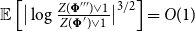 ${\mathbb E}\left [ {\big |\log \frac {Z(\boldsymbol{\Phi }''')\vee 1}{Z(\boldsymbol{\Phi }')\vee 1}\big |^{3/2}}\right] =O(1)$
.
${\mathbb E}\left [ {\big |\log \frac {Z(\boldsymbol{\Phi }''')\vee 1}{Z(\boldsymbol{\Phi }')\vee 1}\big |^{3/2}}\right] =O(1)$
.
Proof. We proceed similarly as in the proof of Lemma 6.1. The construction in CPL3 ensures that
 $\boldsymbol{\Phi }'''$
contains one additional variable
$\boldsymbol{\Phi }'''$
contains one additional variable
 $x_{n+1}$
and
$x_{n+1}$
and
 $\boldsymbol{\Delta }'''\sim \textrm {Po}(d)$
new clauses
$\boldsymbol{\Delta }'''\sim \textrm {Po}(d)$
new clauses
 $b_1,\ldots ,b_{\boldsymbol{\Delta }'''}$
that each contain
$b_1,\ldots ,b_{\boldsymbol{\Delta }'''}$
that each contain
 $x_{n+1}$
and
$x_{n+1}$
and
 $k-1$
other variables. Let
$k-1$
other variables. Let
 $\boldsymbol{x}_{1,1},\ldots ,\boldsymbol{x}_{1,k-1},\ldots ,\boldsymbol{x}_{\boldsymbol{\Delta }''',1},\ldots ,\boldsymbol{x}_{\boldsymbol{\Delta }''',k-1}\in \{x_1,\ldots ,x_n\}$
be the variables among
$\boldsymbol{x}_{1,1},\ldots ,\boldsymbol{x}_{1,k-1},\ldots ,\boldsymbol{x}_{\boldsymbol{\Delta }''',1},\ldots ,\boldsymbol{x}_{\boldsymbol{\Delta }''',k-1}\in \{x_1,\ldots ,x_n\}$
be the variables among
 $x_1,\ldots ,x_n$
that appear in
$x_1,\ldots ,x_n$
that appear in
 $b_1,\ldots ,b_{\boldsymbol{\Delta }'''}$
and let
$b_1,\ldots ,b_{\boldsymbol{\Delta }'''}$
and let
 $\mathscr{X}=\{\boldsymbol{x}_{1,1},\ldots ,\boldsymbol{x}_{\boldsymbol{\Delta }''',k-1}\}$
. Then
$\mathscr{X}=\{\boldsymbol{x}_{1,1},\ldots ,\boldsymbol{x}_{\boldsymbol{\Delta }''',k-1}\}$
. Then
 \begin{align} 0\leq Z(\boldsymbol{\Phi }'')\leq 2Z(\boldsymbol{\Phi }')\leq 2^{n+1}. \end{align}
Hence, if
 $\boldsymbol{\Phi }'$
is unsatisfiable, then so is
$\boldsymbol{\Phi }'$
is unsatisfiable, then so is
 $\boldsymbol{\Phi }'''$
and thus
$\boldsymbol{\Phi }'''$
and thus
 \begin{align} \log \frac {Z(\boldsymbol{\Phi }''')\vee 1}{Z(\boldsymbol{\Phi }')\vee 1} & =0 & & \mbox{ if }Z(\boldsymbol{\Phi }')=0. \end{align}
Furthermore, since
 $\boldsymbol{\Delta }'''\sim \textrm {Po}(d)$
, Bennett’s inequality shows that
$\boldsymbol{\Delta }'''\sim \textrm {Po}(d)$
, Bennett’s inequality shows that
 ${\mathbb P}\left [ {\boldsymbol{\Delta }'''\gt \log n}\right ] =O(n^{-2})$
. Therefore, (6.9) shows that
${\mathbb P}\left [ {\boldsymbol{\Delta }'''\gt \log n}\right ] =O(n^{-2})$
. Therefore, (6.9) shows that
 \begin{align} {\mathbb E}\left [ {\unicode {x1D7D9}\left \{{\boldsymbol{\Delta }'''\gt \log n}\right \}\cdot \left |\log \frac {Z(\boldsymbol{\Phi }''')\vee 1}{Z(\boldsymbol{\Phi }')\vee 1}\right |^{3/2}}\right ] & =o(1). \end{align}
Moreover, since the
 $k-1$
variables among
$k-1$
variables among
 $x_1,\ldots ,x_n$
that appear in the clauses
$x_1,\ldots ,x_n$
that appear in the clauses
 $b_1,\ldots ,b_{\Delta '''}$
are chosen uniformly and independently, a simple balls-into-bins argument shows that
$b_1,\ldots ,b_{\Delta '''}$
are chosen uniformly and independently, a simple balls-into-bins argument shows that
 \begin{align} {\mathbb P}\left [ {|\mathscr{X}|\leq (k-1)(\boldsymbol{\Delta }''-1)\mid \boldsymbol{\Delta }''\leq \log n}\right ] & =\tilde O(n^{-2}). \end{align}
Hence, consider the event
 \begin{align*} \mathfrak{G} & =\left \{{Z(\boldsymbol{\Phi }')\gt 0,\,\boldsymbol{\Delta }'''\leq \log n,\,|\mathscr{X}|\gt (k-1)(\boldsymbol{\Delta }''-1)}\right \}. \end{align*}
Combining (6.9)–(6.12), we obtain
 \begin{align} {\mathbb E}\left [ {(1-\unicode {x1D7D9}\mathfrak{G})\cdot \left |\log \frac {Z(\boldsymbol{\Phi }''')\vee 1}{Z(\boldsymbol{\Phi }')\vee 1}\right |^{3/2}}\right ] & =o(1). \end{align}
Furthermore, if the event
 $\mathfrak{G}$
occurs, then there exists a set
$\mathfrak{G}$
occurs, then there exists a set
 $\mathscr{L}\subseteq \{x,\neg x\,:\,x\in \mathscr{X}\}$
of literals such that each clause
$\mathscr{L}\subseteq \{x,\neg x\,:\,x\in \mathscr{X}\}$
of literals such that each clause
 $b_i$
,
$b_i$
,
 $1\leq i\leq \boldsymbol{\Delta }'''$
, contains a literal
$1\leq i\leq \boldsymbol{\Delta }'''$
, contains a literal
 $l\in \mathscr{L}$
and such that
$l\in \mathscr{L}$
and such that
 $\{x,\neg x\}\not \subseteq \mathscr{L}$
for all
$\{x,\neg x\}\not \subseteq \mathscr{L}$
for all
 $x\in \mathscr{X}$
. Hence, with
$x\in \mathscr{X}$
. Hence, with
 $\skew9\bar{\mathscr{L}}=\skew9\bar{\mathscr{L}}_{\boldsymbol{\Phi }'}$
the output of
$\skew9\bar{\mathscr{L}}=\skew9\bar{\mathscr{L}}_{\boldsymbol{\Phi }'}$
the output of
 $\texttt {PULP}$
on
$\texttt {PULP}$
on
 $(\boldsymbol{\Phi }',\mathscr{L})$
, Lemma 2.8 shows that
$(\boldsymbol{\Phi }',\mathscr{L})$
, Lemma 2.8 shows that
 \begin{align} {\mathbb E}\left [ {\unicode {x1D7D9}\mathfrak{G}\cdot \left |\log \frac {Z(\boldsymbol{\Phi }''')\vee 1}{Z(\boldsymbol{\Phi }')\vee 1}\right |^{3/2}}\right ] & \leq {\mathbb E}\left [ {\unicode {x1D7D9}\mathfrak{G}\cdot |\skew9\bar{\mathscr{L}}|^{3/2}}\right ] . \end{align}
Furthermore, since the clauses
 $b_1,\ldots ,b_{\boldsymbol{\Delta }'''}$
are drawn independently of
$b_1,\ldots ,b_{\boldsymbol{\Delta }'''}$
are drawn independently of
 $\boldsymbol{\Phi }'''$
, Lemma 2.10 shows that there exists
$\boldsymbol{\Phi }'''$
, Lemma 2.10 shows that there exists
 $C=C(d,k)\gt 0$
such that
$C=C(d,k)\gt 0$
such that
 \begin{align} {\mathbb E}\left [ {\unicode {x1D7D9}\mathfrak{G}\cdot |\skew9\bar{\mathscr{L}}|^{3/2}\mid \boldsymbol{\Delta }'''}\right ] & \leq C\cdot (\boldsymbol{\Delta }''')^{3/2}. \end{align}
Finally, since
 $\boldsymbol{\Delta }'''\sim \textrm {Po}(d)$
, the assertion follows from (6.13), (6.14) and (6.15).
$\boldsymbol{\Delta }'''\sim \textrm {Po}(d)$
, the assertion follows from (6.13), (6.14) and (6.15).
6.2 Proof of Proposition 2.11
Let
 $\pi _{d,k}^{(\ell )}=\mathrm{BP}_{d,k}^\ell (\delta _{1/2})$
be the result of an
$\pi _{d,k}^{(\ell )}=\mathrm{BP}_{d,k}^\ell (\delta _{1/2})$
be the result of an
 $\ell$
-fold application of the operator
$\ell$
-fold application of the operator
 $\mathrm{BP}_{d,k}$
from (1.3) to the point mass at
$\mathrm{BP}_{d,k}$
from (1.3) to the point mass at
 $1/2$
. Also recall from (2.7) that
$1/2$
. Also recall from (2.7) that
 $\boldsymbol{\pi }_n'$
denotes the empirical distribution of the marginals
$\boldsymbol{\pi }_n'$
denotes the empirical distribution of the marginals
 $({\mathbb P}[\boldsymbol{\sigma }_{\boldsymbol{\Phi }'}(x_i)=1\mid \boldsymbol{\Phi }'])_{1\leq i\leq n}$
.
$({\mathbb P}[\boldsymbol{\sigma }_{\boldsymbol{\Phi }'}(x_i)=1\mid \boldsymbol{\Phi }'])_{1\leq i\leq n}$
.
Lemma 6.3.
Suppose that
 $d\lt d_{\mathrm{uniq}}(k)$
. For any
$d\lt d_{\mathrm{uniq}}(k)$
. For any
 $\varepsilon \gt 0$
there exists
$\varepsilon \gt 0$
there exists
 $\ell _0=\ell _0(d,k,\varepsilon )\gt 0$
such that for all
$\ell _0=\ell _0(d,k,\varepsilon )\gt 0$
such that for all
 $\ell \geq \ell _0$
we have
$\ell \geq \ell _0$
we have
 \begin{equation*}{\mathbb E}\left[W_1 \left(\boldsymbol{\pi }_n',\pi _{d,k}^{(\ell )} \right)\mid Z(\boldsymbol{\Phi }')\gt 0 \right]\lt \varepsilon +o(1).\end{equation*}
Proof. Assume that
 $\ell \geq \ell _0$
for a large enough
$\ell \geq \ell _0$
for a large enough
 $\ell _0=\ell _0(d,k,\varepsilon )\gt 0$
. Since
$\ell _0=\ell _0(d,k,\varepsilon )\gt 0$
. Since
 $d\lt d_{\mathrm{uniq}}(k)$
and since
$d\lt d_{\mathrm{uniq}}(k)$
and since
 $\mathbb{T}=\mathbb{T}_{d,k}$
is a Galton-Watson tree in which every variable node has
$\mathbb{T}=\mathbb{T}_{d,k}$
is a Galton-Watson tree in which every variable node has
 $\textrm {Po}(d)$
clause nodes as offspring and the offspring of every clause node consists of
$\textrm {Po}(d)$
clause nodes as offspring and the offspring of every clause node consists of
 $k-1$
variable nodes, there exists a set
$k-1$
variable nodes, there exists a set
 $\mathscr{T}_\ell$
of trees, with
$\mathscr{T}_\ell$
of trees, with
 $|\mathscr{T}_\ell |=O(1)$
, such that the following hold:
$|\mathscr{T}_\ell |=O(1)$
, such that the following hold:
-
T0: for every
$T\in \mathscr{T}_\ell$
we have
${\mathbb P}\left [ {\mathbb{T}^{(\ell )}=T}\right ] \gt 0$
. -
T1:
${\mathbb P}\left [ {\mathbb{T}^{(\ell )}\in \mathscr{T}_\ell }\right ] \gt 1-\varepsilon$
. -
T2: given
$\mathbb{T}^{(\ell )}\in \mathscr{T}_\ell$
we have
\begin{align*} \max _{\tau \in S(\mathbb{T}^{(\ell )})}\left |{{\mathbb P}\left [ {\boldsymbol{\tau }^{(\ell )}(\mathfrak{x})=1\mid \mathbb{T}^{(\ell )}}\right ] -{\mathbb P}\left [ {\boldsymbol{\tau }^{(\ell )}(\mathfrak{x})=1\mid \mathbb{T}^{(\ell )},\,\forall x\in \partial ^{2\ell }\mathfrak{x}\,:\,\boldsymbol{\tau }^{(\ell )}(x)=\tau (x)}\right ] }\right | & \lt \varepsilon . \end{align*}


For a variable node
 $x_i$
of
$x_i$
of
 $\boldsymbol{\Phi }'$
obtain
$\boldsymbol{\Phi }'$
obtain
 $\boldsymbol{\phi }'_{\ell }(x_i)$
from
$\boldsymbol{\phi }'_{\ell }(x_i)$
from
 $\boldsymbol{\Phi }'$
by deleting all variables and clauses at distance greater than
$\boldsymbol{\Phi }'$
by deleting all variables and clauses at distance greater than
 $2\ell$
from
$2\ell$
from
 $x_i$
. We consider
$x_i$
. We consider
 $x_i$
being the root of
$x_i$
being the root of
 $\boldsymbol{\phi }'_{\ell }(x_i)$
. Moreover, for a tree
$\boldsymbol{\phi }'_{\ell }(x_i)$
. Moreover, for a tree
 $T\in \mathscr{T}_\ell$
let
$T\in \mathscr{T}_\ell$
let
 $\mathscr{V}_T$
be the set of variable nodes
$\mathscr{V}_T$
be the set of variable nodes
 $x_i$
,
$x_i$
,
 $1\leq i\leq n$
, such that
$1\leq i\leq n$
, such that
 $\boldsymbol{\phi }'_{\ell }(x_i)\cong T$
; thus, there is an isomorphism of the CNFs
$\boldsymbol{\phi }'_{\ell }(x_i)\cong T$
; thus, there is an isomorphism of the CNFs
 $T$
and
$T$
and
 $\boldsymbol{\phi }'_\ell (x_i)$
that maps the root
$\boldsymbol{\phi }'_\ell (x_i)$
that maps the root
 $\mathfrak{x}$
of
$\mathfrak{x}$
of
 $T$
to
$T$
to
 $x_i$
. Consider the event
$x_i$
. Consider the event
 \begin{align} \mathfrak T_\ell & =\left \{{\sum _{T\in \mathscr{T}_\ell }\left |{{\mathbb P}\left [ {\mathbb{T}^{(\ell )}\cong T}\right ] -|\mathscr{V}_T|/n}\right |\lt \varepsilon }\right \}. \end{align}
Then Corollary 3.7 implies that
 \begin{align} {\mathbb P}\left [ {\mathfrak T_\ell }\right ] =1-o(1) \quad \mbox{for every }\ell \geq 0. \end{align}
We now claim that
 \begin{align} \left |{{\mathbb P}\left [ {\boldsymbol{\tau }^{(\ell )}(\mathfrak{x})=1\mid \mathbb{T}^{(\ell )}=T}\right ] -{\mathbb P}\left [ {\boldsymbol{\sigma }_{\boldsymbol{\Phi }'}(x_i)=1\mid \boldsymbol{\Phi }'}\right ] }\right |\lt \varepsilon \quad \mbox{ for all }T\in \mathscr{T}_\ell ,\,x_i\in \mathscr{V}_T. \end{align}
To see this, let
 $S_\ell (\boldsymbol{\Phi }',x_i)$
be the set of all assignments
$S_\ell (\boldsymbol{\Phi }',x_i)$
be the set of all assignments
 $\sigma \in \{\pm 1\}^{\partial ^{2\ell }x_i}$
of the variables at distance
$\sigma \in \{\pm 1\}^{\partial ^{2\ell }x_i}$
of the variables at distance
 $2\ell$
from
$2\ell$
from
 $x_i$
in
$x_i$
in
 $\boldsymbol{\Phi }'$
such that there exists a satisfying assignment
$\boldsymbol{\Phi }'$
such that there exists a satisfying assignment
 $\sigma '\in S(\boldsymbol{\Phi }')$
with
$\sigma '\in S(\boldsymbol{\Phi }')$
with
 $\sigma '(y)=\sigma (y)$
for all
$\sigma '(y)=\sigma (y)$
for all
 $y\in \partial ^{2\ell }x_i$
. Then the law of total probability shows that
$y\in \partial ^{2\ell }x_i$
. Then the law of total probability shows that
 \begin{align} {\mathbb P}\left [ {\boldsymbol{\sigma }_{\boldsymbol{\Phi }'}(x_i)=1\mid \boldsymbol{\Phi }'}\right ] & =\sum _{\sigma \in S_\ell (\boldsymbol{\Phi }',x_i)}{\mathbb P}\left [ {\boldsymbol{\sigma }_{\boldsymbol{\Phi }'}(x_i)=1\mid \boldsymbol{\Phi }',\,\forall y\in \partial ^{2\ell }x_i \,:\, \boldsymbol{\sigma }_{\boldsymbol{\Phi }'}(y)=\sigma (y)}\right ]\nonumber\\ & \qquad {\mathbb P}\left [ {\forall y\in \partial ^{2\ell }x_i \,:\, \boldsymbol{\sigma }_{\boldsymbol{\Phi }'}(y)=\sigma (y)\mid \boldsymbol{\Phi }'}\right ] . \end{align}
Further, since for
 $T\in \mathscr{T}_\ell$
and
$T\in \mathscr{T}_\ell$
and
 $x_i\in \mathscr{V}_T$
we have
$x_i\in \mathscr{V}_T$
we have
 $\boldsymbol{\phi }_\ell '(x_i)\cong T$
, condition T2 implies that
$\boldsymbol{\phi }_\ell '(x_i)\cong T$
, condition T2 implies that
 \begin{align} \left |{{\mathbb P}\left [ {\boldsymbol{\sigma }_{\boldsymbol{\Phi }'}(x_i)=1\mid \boldsymbol{\Phi }',\,\forall y\in \partial ^{2\ell }x_i \,:\, \boldsymbol{\sigma }_{\boldsymbol{\Phi }'}(y)=\sigma (y)}\right ] -{\mathbb P}\left [ {\boldsymbol{\tau }^{(\ell )}(\mathfrak{x})=1\mid \mathbb{T}^{(\ell )}=T}\right ] }\right | & \lt \varepsilon . \end{align}
Combining (6.19) and (6.20), we obtain (6.18).
To complete the proof, we recall from Fact 4.2 that
 $\pi _{d,k}^{(\ell )}$
is precisely the distribution of
$\pi _{d,k}^{(\ell )}$
is precisely the distribution of
 ${\mathbb P}\left [ {\boldsymbol{\tau }^{(\ell )}(\mathfrak{x})=1\mid \mathbb{T}^{(\ell )}}\right ]$
. Therefore, coupling the formulas
${\mathbb P}\left [ {\boldsymbol{\tau }^{(\ell )}(\mathfrak{x})=1\mid \mathbb{T}^{(\ell )}}\right ]$
. Therefore, coupling the formulas
 $\mathbb{T}^{(\ell )}, \boldsymbol{\Phi }'$
on the event
$\mathbb{T}^{(\ell )}, \boldsymbol{\Phi }'$
on the event
 $\mathfrak T_\ell$
we have
$\mathfrak T_\ell$
we have

Combining this bound with (6.17) completes the proof.
Proof of Proposition
2.11. The first assertion follows from Proposition 2.1, Lemma 6.3 and the fact that, since
 $0\lt d \lt d_{\mathrm{uniq}}(k) \lt d_{\mathrm{sat}}(k)$
, we have that
$0\lt d \lt d_{\mathrm{uniq}}(k) \lt d_{\mathrm{sat}}(k)$
, we have that
 ${\mathbb P}\left [ {Z(\boldsymbol{\Phi }')\gt 0}\right ] =1-o(1)$
.
${\mathbb P}\left [ {Z(\boldsymbol{\Phi }')\gt 0}\right ] =1-o(1)$
.
The second follows a routine argument, which we present below for the case
 $\ell = 2$
and it is standard to extend to any finite
$\ell = 2$
and it is standard to extend to any finite
 $\ell$
(see [Reference Coja-Oghlan and Perkins29, Proposition2.5]). Let
$\ell$
(see [Reference Coja-Oghlan and Perkins29, Proposition2.5]). Let
 $t= \Theta (\log \log n)$
and recall the definitions of
$t= \Theta (\log \log n)$
and recall the definitions of
 $\boldsymbol{\phi }'_{t}(x_i)$
,
$\boldsymbol{\phi }'_{t}(x_i)$
,
 $\mathscr{T}_{t}$
and
$\mathscr{T}_{t}$
and
 $S_t(\boldsymbol{\Phi }',x_i)$
from the proof of Lemma 6.3. Consider the event
$S_t(\boldsymbol{\Phi }',x_i)$
from the proof of Lemma 6.3. Consider the event
 $\mathfrak{D} = \{\boldsymbol{\phi }'_{t}(x_1), \boldsymbol{\phi }'_{t}(x_2) \text{ are disjoint tree formulas}\}$
.
$\mathfrak{D} = \{\boldsymbol{\phi }'_{t}(x_1), \boldsymbol{\phi }'_{t}(x_2) \text{ are disjoint tree formulas}\}$
.
From Lemma 3.5, we have that
 ${\mathbb P}\left [ {\mathfrak{D}}\right ] = 1 - o(1)$
. On the event
${\mathbb P}\left [ {\mathfrak{D}}\right ] = 1 - o(1)$
. On the event
 $\mathfrak{D}$
, Lemma 6.3 implies that for every
$\mathfrak{D}$
, Lemma 6.3 implies that for every
 $\sigma _1, \sigma _2 \in \{\pm 1\}$
, and
$\sigma _1, \sigma _2 \in \{\pm 1\}$
, and
 $\tau _1 \in S_t(\boldsymbol{\Phi }',x_1), \tau _2 \in S_t(\boldsymbol{\Phi }',x_2)$
we have
$\tau _1 \in S_t(\boldsymbol{\Phi }',x_1), \tau _2 \in S_t(\boldsymbol{\Phi }',x_2)$
we have
 \begin{align} |{\mathbb P}\left [ {\boldsymbol{\sigma }_{\boldsymbol{\Phi }'}(x_i)=\sigma _i\mid \boldsymbol{\Phi }',\,\forall y\in \partial ^{2t}x_i \,:\, \boldsymbol{\sigma }_{\boldsymbol{\Phi }'}(y)=\tau _i(y)}\right ] - {\mathbb P}\left [ {\boldsymbol{\sigma }_{\boldsymbol{\Phi }'}(x_i)=\sigma _i\mid \boldsymbol{\Phi }'}\right ] | = o(1) , & & \text{ for } i=1,2 . \end{align}
Therefore, from the law of total probability and the triangle inequality we see that for every
 $\sigma _1,\sigma _2 \in \{\pm 1\}$
 \begin{align*} & \left |{{\mathbb P}\left [ {\boldsymbol{\sigma }_{\boldsymbol{\Phi }'}(x_1)=\sigma _1, \boldsymbol{\sigma }_{\boldsymbol{\Phi }'}(x_2)=\sigma _2\mid \boldsymbol{\Phi }'}\right ] -{\mathbb P}\left [ {\boldsymbol{\sigma }_{\boldsymbol{\Phi }'}(x_1)=\sigma _1\mid \boldsymbol{\Phi }'}\right ] {\mathbb P}\left [ {\boldsymbol{\sigma }_{\boldsymbol{\Phi }'}(x_2)=\sigma _2\mid \boldsymbol{\Phi }'}\right ] }\right | \\ & \,\,\, \le \Big |\!\left |{{\mathbb P}\left [ {\boldsymbol{\sigma }_{\boldsymbol{\Phi }'}(x_1)=\sigma _1\mid \boldsymbol{\Phi }', \boldsymbol{\sigma }_{\boldsymbol{\Phi }'}(x_2)= \sigma _2 }\right ] - {\mathbb E}_{\tau _1, \tau _2}\left [ {{\mathbb P}\left [ {\boldsymbol{\sigma }_{\boldsymbol{\Phi }'}(x_1)=\sigma _1, \boldsymbol{\sigma }_{\boldsymbol{\Phi }'}(x_2)=\sigma _2\mid \boldsymbol{\Phi }',\tau _1, \tau _2}\right ] }\right ] }\right |\\ & \qquad- \left |{\mathbb E}_{\tau _1, \tau _2}\left [ {{\mathbb P}\left [ {\boldsymbol{\sigma }_{\boldsymbol{\Phi }'}(x_1)=\sigma _1\mid \boldsymbol{\Phi }',\tau _1}\right ] {\mathbb P}\left [ {\boldsymbol{\sigma }_{\boldsymbol{\Phi }'}(x_2)=\sigma _2\mid \boldsymbol{\Phi }', \tau _2}\right ] }\right ] -{\mathbb P}\left [ {\boldsymbol{\sigma }_{\boldsymbol{\Phi }'}(x_2)=\sigma _2\mid \boldsymbol{\Phi }'}\right ]\right.\\ & \,\,\, \left.\qquad {\mathbb P}\left [ {\boldsymbol{\sigma }_{\boldsymbol{\Phi }'}(x_2)=\sigma _2\mid \boldsymbol{\Phi }'}\right ] \right | \Big | \\ & \quad = \Big |\left |{\mathbb E}_{\tau _1, \tau _2}\left [ {{\mathbb P}\left [ {\boldsymbol{\sigma }_{\boldsymbol{\Phi }'}(x_1)=\sigma _1\mid \boldsymbol{\Phi }',\tau _1}\right ] {\mathbb P}\left [ {\boldsymbol{\sigma }_{\boldsymbol{\Phi }'}(x_2)=\sigma _2\mid \boldsymbol{\Phi }', \tau _2}\right ] }\right ] -{\mathbb P}\left [ {\boldsymbol{\sigma }_{\boldsymbol{\Phi }'}(x_2)=\sigma _2\mid \boldsymbol{\Phi }'}\right ]\right.\\ & \,\,\, \left.\qquad {\mathbb P}\left [ {\boldsymbol{\sigma }_{\boldsymbol{\Phi }'}(x_2)=\sigma _2\mid \boldsymbol{\Phi }'}\right ] \right | \Big | \\ & \,\,\, \le {\mathbb E}_{\tau _1}\left |{{\mathbb P}\left [ {\boldsymbol{\sigma }_{\boldsymbol{\Phi }'}(x_1)=\sigma _1 \mid \boldsymbol{\Phi }',\tau _1}\right ] - {\mathbb P}\left [ {\boldsymbol{\sigma }_{\boldsymbol{\Phi }'}(x_1)=\sigma _1 \mid \boldsymbol{\Phi }'}\right ] }\right | + {\mathbb E}_{\tau _2}\left |{\mathbb P}\left [ {\boldsymbol{\sigma }_{\boldsymbol{\Phi }'}(x_2)=\sigma _2\mid \boldsymbol{\Phi }',\tau _2}\right ] \right.\\ \quad & \left.\qquad - {\mathbb P}\left [ {\boldsymbol{\sigma }_{\boldsymbol{\Phi }'}(x_2)=\sigma _2\mid \boldsymbol{\Phi }'}\right ] \right | \\ & \,\,\,= o(1). & & \!\!\!\!\!\!\!\!\!\!\!\!\!\!\!\!\!\!\!\!\!\!\!\!\!\!\!\mbox{[by (6.21)]} \end{align*}
Summing over the four sign combinations of
 $\sigma _1, \sigma _2$
gives the desired result.
$\sigma _1, \sigma _2$
gives the desired result.
6.3 Proof of Proposition 2.5
As in the proof of Lemma 6.1 let
 $c_1,\ldots ,c_{\boldsymbol{\Delta }''}$
be the new clauses added by CPL2 and let
$c_1,\ldots ,c_{\boldsymbol{\Delta }''}$
be the new clauses added by CPL2 and let
 $\boldsymbol{x}_{1,1},\ldots ,\boldsymbol{x}_{1,k},\ldots ,\boldsymbol{x}_{\boldsymbol{\Delta }'',1},\ldots ,\boldsymbol{x}_{\boldsymbol{\Delta }'',k}$
be their constituent variables. Let
$\boldsymbol{x}_{1,1},\ldots ,\boldsymbol{x}_{1,k},\ldots ,\boldsymbol{x}_{\boldsymbol{\Delta }'',1},\ldots ,\boldsymbol{x}_{\boldsymbol{\Delta }'',k}$
be their constituent variables. Let
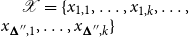 $\mathscr{X}=\{\boldsymbol{x}_{1,1},\ldots ,\boldsymbol{x}_{1,k},\ldots , \boldsymbol{x}_{\boldsymbol{\Delta }'',1},\ldots ,\boldsymbol{x}_{\boldsymbol{\Delta }'',k}\}$
. For
$\mathscr{X}=\{\boldsymbol{x}_{1,1},\ldots ,\boldsymbol{x}_{1,k},\ldots , \boldsymbol{x}_{\boldsymbol{\Delta }'',1},\ldots ,\boldsymbol{x}_{\boldsymbol{\Delta }'',k}\}$
. For
 $\varepsilon \gt 0$
and
$\varepsilon \gt 0$
and
 $z \in \mathbb{R}$
define
$z \in \mathbb{R}$
define
 $\lambda _\varepsilon (z) = \log (z\vee \varepsilon )$
. Finally, let
$\lambda _\varepsilon (z) = \log (z\vee \varepsilon )$
. Finally, let
 $(\boldsymbol{s}_i)_{i\geq 0}$
be a sequence of uniformly random
$(\boldsymbol{s}_i)_{i\geq 0}$
be a sequence of uniformly random
 $\pm 1$
-valued random variables, mutually independent and independent of all other randomness.
$\pm 1$
-valued random variables, mutually independent and independent of all other randomness.
Lemma 6.4.
Assume that
 $d\lt d_{\mathrm{uniq}}(k)$
. There exists
$d\lt d_{\mathrm{uniq}}(k)$
. There exists
 $B=B(d,k)\gt 0$
such that for all
$B=B(d,k)\gt 0$
such that for all
 $0\lt \varepsilon \lt 1$
we have
$0\lt \varepsilon \lt 1$
we have
 \begin{align*} \limsup _{n\to \infty }{\mathbb E}\left [ {\left ({\sum _{i=1}^{\boldsymbol{\Delta }''}\lambda _\varepsilon \left ({1-\prod _{j=1}^k {\mathbb P}\left [ {\boldsymbol{\sigma }(\boldsymbol{x}_{i,j})\neq \mathrm{sign}(\boldsymbol{x}_{i,j},c_i)\mid \boldsymbol{\Phi }'}\right ] }\right )}\right )^2\mid Z(\boldsymbol{\Phi }')\gt 0}\right ] \leq B. \end{align*}
Proof. Given
 $Z(\boldsymbol{\Phi }')\gt 0$
we have
$Z(\boldsymbol{\Phi }')\gt 0$
we have
 \begin{align} 0 & \geq \lambda _\varepsilon \left ({1-\prod _{j=1}^k {\mathbb P}\left [ {\boldsymbol{\sigma }(\boldsymbol{x}_{1,j})\neq \mathrm{sign}(\boldsymbol{x}_{1,j}, c_1)\mid \boldsymbol{\Phi }'}\right ] }\right )\geq \lambda _\varepsilon \left ({1-{\mathbb P}\left [ {\boldsymbol{\sigma }(\boldsymbol{x}_{1,1})\neq \mathrm{sign}(\boldsymbol{x}_{1,1}, c_1)\mid \boldsymbol{\Phi }'}\right ] }\right ). \end{align}
Recalling that
 $\boldsymbol{\Delta }''\sim \textrm {Po}(d(k-1)/k)$
, we combine (6.22) with Cauchy-Schwarz to obtain
$\boldsymbol{\Delta }''\sim \textrm {Po}(d(k-1)/k)$
, we combine (6.22) with Cauchy-Schwarz to obtain
 $B'=B'(d,k)\gt 0$
such that
$B'=B'(d,k)\gt 0$
such that
 \begin{align} \nonumber {\mathbb E} & \left [ {\left ({\sum _{i=1}^{\boldsymbol{\Delta }''}\lambda _\varepsilon \left ({1-\prod _{j=1}^k{\mathbb P}\left [ {\boldsymbol{\sigma }(\boldsymbol{x}_{i,j})\neq \mathrm{sign}(\boldsymbol{x}_{i,j}, c_i)\mid \boldsymbol{\Phi }'}\right ] }\right )}\right )^2\mid Z(\boldsymbol{\Phi }')\gt 0}\right ] \\ & \leq B'\cdot {\mathbb E}\left [ {\lambda _\varepsilon \left ({1-{\mathbb P}\left [ {\boldsymbol{\sigma }(\boldsymbol{x}_{1,1})\neq \mathrm{sign}(\boldsymbol{x}_{1,1}, c_1)\mid \boldsymbol{\Phi }'}\right ] }\right )^2\mid Z(\boldsymbol{\Phi }')\gt 0}\right ] . \end{align}
Further, since the function
 $\lambda _\varepsilon$
is bounded and continuous for every
$\lambda _\varepsilon$
is bounded and continuous for every
 $\varepsilon \gt 0$
and since
$\varepsilon \gt 0$
and since
 $\mathrm{sign}(\boldsymbol{x}_{1,1}, c_1)$
is chosen independently of
$\mathrm{sign}(\boldsymbol{x}_{1,1}, c_1)$
is chosen independently of
 $\boldsymbol{\Phi }'$
, Proposition 2.11 shows that for any
$\boldsymbol{\Phi }'$
, Proposition 2.11 shows that for any
 $\varepsilon \gt 0$
,
$\varepsilon \gt 0$
,
 \begin{align} \nonumber {\mathbb E}\left [ {\lambda _\varepsilon \left ({1-{\mathbb P}\left [ {\boldsymbol{\sigma }(\boldsymbol{x}_{1,1})\neq \mathrm{sign}(\boldsymbol{x}_{1,1}, c_1)\mid \boldsymbol{\Phi }'}\right ] }\right )^2\mid Z(\boldsymbol{\Phi }')\gt 0}\right ] & = {\mathbb E}\big [ {\lambda _\varepsilon \big ({\boldsymbol{\mu }_{\pi _{d,k},1,1}}\big)^2}\big ] +o(1) \\ & \leq {\mathbb E}\big [ {\log \big ({\boldsymbol{\mu }_{\pi _{d,k},1,1}}\big)^2}\big] +o(1). \end{align}
Since Proposition 2.1 shows that
 ${\mathbb E}\big[ {\log \big ({\boldsymbol{\mu }_{\pi _{d,k},1,1}}\big )^2}\big] =O(1)$
, the assertion follows from (6.23) and (6.24).
${\mathbb E}\big[ {\log \big ({\boldsymbol{\mu }_{\pi _{d,k},1,1}}\big )^2}\big] =O(1)$
, the assertion follows from (6.23) and (6.24).
Lemma 6.5.
Assume that
 $d\lt d_{\mathrm{uniq}}(k)$
. For any
$d\lt d_{\mathrm{uniq}}(k)$
. For any
 $\delta \gt 0$
there exists
$\delta \gt 0$
there exists
 $\varepsilon _0\gt 0$
such that for all
$\varepsilon _0\gt 0$
such that for all
 $\varepsilon _0\gt \varepsilon \gt 0$
we have
$\varepsilon _0\gt \varepsilon \gt 0$
we have
 \begin{align*} \limsup _{n\to \infty }\left |{{\mathbb E}\left [ {\log \frac {Z(\boldsymbol{\Phi }'')\vee 1}{Z(\boldsymbol{\Phi }')\vee 1}}\right ] -\frac {d(k-1)}k{\mathbb E}\left [ {\lambda _\varepsilon \left ({1-\prod _{j=1}^k{\mathbb P}\left [ {\boldsymbol{\sigma }(x_j)=\boldsymbol{s}_j\mid \boldsymbol{\Phi }'}\right ] }\right )\mid Z(\boldsymbol{\Phi }')\gt 0}\right ] }\right |\lt \delta . \end{align*}
Proof. We choose small enough
 $\xi =\xi (d,k,\delta )\gt \zeta (\xi )\gt \eta =\eta (\zeta )\gt \varepsilon _0=\varepsilon _0(\eta )\gt 0$
, let
$\xi =\xi (d,k,\delta )\gt \zeta (\xi )\gt \eta =\eta (\zeta )\gt \varepsilon _0=\varepsilon _0(\eta )\gt 0$
, let
 $0\lt \varepsilon \lt \varepsilon _0$
and assume that
$0\lt \varepsilon \lt \varepsilon _0$
and assume that
 $n\ge n_0(\varepsilon )$
is large enough. Also let
$n\ge n_0(\varepsilon )$
is large enough. Also let
 $\gamma =\gamma (n)=o(1)$
be a sequence that tends to zero sufficiently slowly. Additionally, let
$\gamma =\gamma (n)=o(1)$
be a sequence that tends to zero sufficiently slowly. Additionally, let
 $\mathfrak{E}$
be the event that all of the following conditions occur.
$\mathfrak{E}$
be the event that all of the following conditions occur.
-
E1:
$Z(\boldsymbol{\Phi }')\gt 0.$
-
E2:
$\boldsymbol{\Delta }''\leq \zeta ^{-1}.$
-
E3:
$|\mathscr{X}|=k\boldsymbol{\Delta }''.$
-
E4:
$\max _{x\in \mathscr{X},s\in \{\pm 1\}}{\mathbb P}[\boldsymbol{\sigma }(x)=s\mid \boldsymbol{\Phi }']\leq 1-\eta .$
-
E5:
$\sum _{\tau \in \{\pm 1\}^{\mathscr{X}}}\left |{{\mathbb P}[\forall x\in \mathscr{X}:\boldsymbol{\sigma }(x)=\tau (x)\mid \boldsymbol{\Phi }']-\prod _{x\in \mathscr{X}}{\mathbb P}[\boldsymbol{\sigma }(x)=\tau (x)\mid \boldsymbol{\Phi }']}\right |\lt \gamma .$


We claim that
 \begin{align} {\mathbb P}\left [ {\mathfrak{E}}\right ] & \geq 1-2\xi +o(1). \end{align}
Indeed, since
 $0\lt d \lt d_{\mathrm{uniq}}(k) \lt d_{\mathrm{sat}}(k)$
, we have that
$0\lt d \lt d_{\mathrm{uniq}}(k) \lt d_{\mathrm{sat}}(k)$
, we have that
 ${\mathbb P}\left [ {Z(\boldsymbol{\Phi }')\gt 0}\right ] =1-o(1)$
. Moreover, since
${\mathbb P}\left [ {Z(\boldsymbol{\Phi }')\gt 0}\right ] =1-o(1)$
. Moreover, since
 $\boldsymbol{\Delta }^{\prime \prime }\sim \textrm {Po}(d(k-1)/k)$
, Markov’s inequality shows that
$\boldsymbol{\Delta }^{\prime \prime }\sim \textrm {Po}(d(k-1)/k)$
, Markov’s inequality shows that
 ${\mathbb P}\left [ {\boldsymbol{\Delta }''\gt \zeta ^{-1}}\right ] \leq \zeta d \lt \xi$
. Further, since the new clauses
${\mathbb P}\left [ {\boldsymbol{\Delta }''\gt \zeta ^{-1}}\right ] \leq \zeta d \lt \xi$
. Further, since the new clauses
 $c_1,\ldots ,c_{\boldsymbol{\Delta }''}$
are chosen independently, we have
$c_1,\ldots ,c_{\boldsymbol{\Delta }''}$
are chosen independently, we have
 ${\mathbb P}\left [ {|\mathscr{X}|=k\boldsymbol{\Delta }''\mid \boldsymbol{\Delta }''\leq \zeta ^{-1}}\right ] =$
 $1-O(1/n)$
.
$1-O(1/n)$
.
Moreover, per Proposition 2.11 we see that the joint distribution on the assignments over
 $\mathscr{X}$
must be approximately the product measure. The tails of the limiting distribution of the latter are controlled by (2.1). Therefore, for small enough
$\mathscr{X}$
must be approximately the product measure. The tails of the limiting distribution of the latter are controlled by (2.1). Therefore, for small enough
 $\eta$
we should have
$\eta$
we should have
 \begin{align*} {\mathbb P}\left [ {\max _{x\in \mathscr{X},s\in \{\pm 1\}}{\mathbb P}[\boldsymbol{\sigma }(x)=s\mid \boldsymbol{\Phi }']\leq 1-\eta \mid \boldsymbol{\Delta }''\leq \zeta ^{-1},\,Z(\boldsymbol{\Phi }')\gt 0}\right ] \geq 1-\xi. \end{align*}
Similarly, Proposition 2.11 shows together with Markov’s inequality that
 \begin{align*} {\mathbb P}\left [ {\textbf {E5}\ \mbox{occurs}\mid \boldsymbol{\Delta }'' \le \zeta ^{-1},\,Z(\boldsymbol{\Phi }')\gt 0}\right ] =1-o(1), \end{align*}
provided that
 $\gamma \to \infty$
sufficiently slowly. Thus, we obtain (6.25).
$\gamma \to \infty$
sufficiently slowly. Thus, we obtain (6.25).
Furthermore, (6.25) implies together with Proposition 2.7 and Hölder’s inequality that
 \begin{align} {\mathbb E}\left |{(1-\unicode {x1D7D9}\mathfrak{E})\cdot \log \frac {Z(\boldsymbol{\Phi }'')}{Z(\boldsymbol{\Phi }')}}\right | & \leq \delta /3+o(1), \end{align}
provided that
 $\xi =\xi (d,k,\delta )\gt 0$
is small enough. Analogously, (6.25), Lemma 6.4 and Cauchy-Schwarz yield
$\xi =\xi (d,k,\delta )\gt 0$
is small enough. Analogously, (6.25), Lemma 6.4 and Cauchy-Schwarz yield
 \begin{align} {\mathbb E}\left |{(1-\unicode {x1D7D9}\mathfrak{E})\lambda _\varepsilon \left ({1-\prod _{j=1}^k{\mathbb P}\left [ {\boldsymbol{\sigma }(x_j)=\boldsymbol{s}_j\mid \boldsymbol{\Phi }'}\right ] }\right )}\right | & \leq \delta /3+o(1). \end{align}
Thus, we confine ourselves to the event
 $\mathfrak{E}$
, on which we have
$\mathfrak{E}$
, on which we have
 $Z(\boldsymbol{\Phi }'),Z(\boldsymbol{\Phi }'')\gt 0$
due to E1, E3, E4 and E5. Hence,
$Z(\boldsymbol{\Phi }'),Z(\boldsymbol{\Phi }'')\gt 0$
due to E1, E3, E4 and E5. Hence,
 \begin{align} \nonumber \log \frac {Z(\boldsymbol{\Phi }'')\vee 1}{Z(\boldsymbol{\Phi }')\vee 1} & =\log \frac {Z(\boldsymbol{\Phi }'')}{Z(\boldsymbol{\Phi }')}= \log \sum _{\tau \in \{\pm 1\}^{\mathscr{X}}}\unicode {x1D7D9}\left \{{\tau \models c_1,\ldots ,c_{\boldsymbol{\Delta }''}}\right \}{\mathbb P}[\forall x\in \mathscr{X}\,:\,\boldsymbol{\sigma }(x)=\tau (x)\mid \boldsymbol{\Phi }']\\ & =\log \sum _{\tau \in \{\pm 1\}^{\mathscr{X}}}\unicode {x1D7D9}\left \{{\tau \models c_1,\ldots ,c_{\boldsymbol{\Delta }''}}\right \}\prod _{x\in \mathscr{X}}{\mathbb P}[\boldsymbol{\sigma }(x)=\tau (x)\mid \boldsymbol{\Phi }']+o(1) & & \!\!\!\!\!\!\!\!\!\!\!\!\!\!\!\!\!\!\!\!\mbox{[by }\textbf {E4, E5}]\nonumber \\ & =\sum _{i=1}^{\boldsymbol{\Delta }''}\log \left [ {1-\prod _{j=1}^k{\mathbb P}\left [ {\boldsymbol{\sigma }(\boldsymbol{x}_{i,j})\neq \mathrm{sign}(\boldsymbol{x}_{i,j},c_i)\mid \boldsymbol{\Phi }'}\right ] }\right ] +o(1) & & \!\!\!\!\!\!\!\!\!\!\!\!\!\mbox{[by }\textbf {E3}]. \end{align}
Further, E4 ensures that for any
 $1\leq i\leq \Delta ''$
,
$1\leq i\leq \Delta ''$
,
 \begin{align} \left |{\log \left [ {1-\prod _{j=1}^k{\mathbb P}\left [ {\boldsymbol{\sigma }(\boldsymbol{x}_{i,j})\neq \mathrm{sign}(\boldsymbol{x}_{i,j},c_i)\mid \boldsymbol{\Phi }'}\right ] }\right ] -\lambda _\varepsilon \left [ {1-\prod _{j=1}^k{\mathbb P}\left [ {\boldsymbol{\sigma }(\boldsymbol{x}_{i,j})\neq \mathrm{sign}(\boldsymbol{x}_{i,j}, c_i)\mid \boldsymbol{\Phi }'}\right ] }\right ] }\right |\lt \xi . \end{align}
Thus, combining (6.28) and (6.29), we obtain
 \begin{align} {\mathbb E}\left |{\unicode {x1D7D9}\mathfrak{E}\left ({\log \frac {Z(\boldsymbol{\Phi }'')\vee 1}{Z(\boldsymbol{\Phi }')\vee 1}-\sum _{i=1}^{\boldsymbol{\Delta }''}\lambda _\varepsilon \left ({1-\prod _{j=1}^k{\mathbb P}\left [ {\boldsymbol{\sigma }(\boldsymbol{x}_{i,j})\neq \mathrm{sign}(\boldsymbol{x}_{i,j}, c_i)\mid \boldsymbol{\Phi }'}\right ] }\right )}\right )}\right | & \lt \delta /3+o(1). \end{align}
Further, combining (6.26) and (6.30) with Lemma 6.4, we obtain
 \begin{align} \left |{{\mathbb E}\left [ {\log \frac {Z(\boldsymbol{\Phi }'')\vee 1}{Z(\boldsymbol{\Phi }')\vee 1}}\right ] {-}{\mathbb E}\left [ {\sum _{i=1}^{\boldsymbol{\Delta }''}\lambda _\varepsilon \left ({1{-}\prod _{j=1}^k{\mathbb P}\left [ {\boldsymbol{\sigma }(\boldsymbol{x}_{i,j})\neq \mathrm{sign}(\boldsymbol{x}_{i,j},c_i)\mid \boldsymbol{\Phi }'}\right ] }\right )\mid Z(\boldsymbol{\Phi }')\gt 0}\right ] }\right | & \!{\lt} \delta {+}o(1). \end{align}
Finally, since the clauses
 $c_1,\ldots ,c_{\boldsymbol{\Delta }''}$
are drawn uniformly and independently and since the distribution of
$c_1,\ldots ,c_{\boldsymbol{\Delta }''}$
are drawn uniformly and independently and since the distribution of
 $\boldsymbol{\Phi }'$
is invariant under permutation of the variable nodes, we find
$\boldsymbol{\Phi }'$
is invariant under permutation of the variable nodes, we find
 \begin{align} \nonumber {\mathbb E} & \left [ {\sum _{i=1}^{\boldsymbol{\Delta }''}\lambda _\varepsilon \left ({1-\prod _{j=1}^k{\mathbb P}\left [ {\boldsymbol{\sigma }(\boldsymbol{x}_{i,j})\neq \mathrm{sign}(\boldsymbol{x}_{i,j},c_i)\mid \boldsymbol{\Phi }'}\right ] \mid Z(\boldsymbol{\Phi }')\gt 0}\right )}\right ] \\ & =\frac {d(k-1)}{k}{\mathbb E}\left [ {\lambda _\varepsilon \left ({1-\prod _{j=1}^k{\mathbb P}\left [ {\boldsymbol{\sigma }(x_j)=\boldsymbol{s}_j}\right ] \mid \boldsymbol{\Phi }'}\right )\mid Z(\boldsymbol{\Phi }')\gt 0}\right ] . \end{align}
Proof of Proposition 2.5. Proposition 2.11 shows together with Lemma 6.5 that
 \begin{align} {\mathbb E}\left [ {\log \frac {Z(\boldsymbol{\Phi }'')\vee 1}{Z(\boldsymbol{\Phi }')\vee 1}}\right ] & =\frac {d(k-1)}k{\mathbb E}\left [ {\lambda _\varepsilon \left ({1-\prod _{j=1}^k\boldsymbol{\mu }_{\pi _{d,k},1,j}}\right )}\right ] +o_\varepsilon (1), \end{align}
with
 $o_\varepsilon (1)$
hiding a term that vanishes in the limit
$o_\varepsilon (1)$
hiding a term that vanishes in the limit
 $\varepsilon \to 0$
. Furthermore, in light of (2.1) the monotone convergence theorem yields
$\varepsilon \to 0$
. Furthermore, in light of (2.1) the monotone convergence theorem yields
 \begin{align} {\mathbb E}\left [ {\log \left ({1-\prod _{j=1}^k\boldsymbol{\mu }_{\pi _{d,k},1,j}}\right )}\right ] & =\lim _{\varepsilon \to 0}{\mathbb E}\left [ {\lambda _\varepsilon \left ({1-\prod _{j=1}^k\boldsymbol{\mu }_{\pi _{d,k},1,j}}\right )}\right ] . \end{align}
6.4 Proof of Proposition 2.6
We adapt the steps from Section 6.3 to the coupling of
 $\boldsymbol{\Phi }'$
,
$\boldsymbol{\Phi }'$
,
 $\boldsymbol{\Phi }'''$
. Recall that the latter is obtained by adding to
$\boldsymbol{\Phi }'''$
. Recall that the latter is obtained by adding to
 $\boldsymbol{\Phi }'$
a single variable
$\boldsymbol{\Phi }'$
a single variable
 $x_{n+1}$
along with
$x_{n+1}$
along with
 $\boldsymbol{\Delta }'''$
clauses
$\boldsymbol{\Delta }'''$
clauses
 $b_1,\ldots ,b_{\boldsymbol{\Delta }'''}$
that each contain
$b_1,\ldots ,b_{\boldsymbol{\Delta }'''}$
that each contain
 $x_{n+1}$
and
$x_{n+1}$
and
 $k-1$
other variables. Thus, let
$k-1$
other variables. Thus, let
 $\boldsymbol{x}_{1,1},\ldots ,\boldsymbol{x}_{1,k-1},\ldots ,\boldsymbol{x}_{\boldsymbol{\Delta }''',1},\ldots ,\boldsymbol{x}_{\boldsymbol{\Delta }''',k-1}\in \{x_1,\ldots ,x_n\}$
be the variables other than
$\boldsymbol{x}_{1,1},\ldots ,\boldsymbol{x}_{1,k-1},\ldots ,\boldsymbol{x}_{\boldsymbol{\Delta }''',1},\ldots ,\boldsymbol{x}_{\boldsymbol{\Delta }''',k-1}\in \{x_1,\ldots ,x_n\}$
be the variables other than
 $x_{n+1}$
that appear in
$x_{n+1}$
that appear in
 $b_1,\ldots ,b_{\boldsymbol{\Delta }'''}$
and let
$b_1,\ldots ,b_{\boldsymbol{\Delta }'''}$
and let
 $\mathscr{X}=\{\boldsymbol{x}_{1,1},\ldots ,\boldsymbol{x}_{\boldsymbol{\Delta }''',k-1}\}$
be the set comprising all these variables.
$\mathscr{X}=\{\boldsymbol{x}_{1,1},\ldots ,\boldsymbol{x}_{\boldsymbol{\Delta }''',k-1}\}$
be the set comprising all these variables.
Lemma 6.6.
Assume that
 $0\lt d\lt d_{\mathrm{uniq}}(k)$
. There exists
$0\lt d\lt d_{\mathrm{uniq}}(k)$
. There exists
 $B=B(d,k)\gt 0$
such that for all
$B=B(d,k)\gt 0$
such that for all
 $0\lt \varepsilon \lt 1$
we have
$0\lt \varepsilon \lt 1$
we have
 \begin{align*} & \limsup _{n\to \infty }{\mathbb E}\left[ \lambda _\varepsilon \left(\sum _{s\in \{\pm 1\}}\prod _{i=1}^{\boldsymbol{\Delta }'''}\left(1-\unicode {x1D7D9}\{\mathrm{sign}(x_{n+1},b_i)\neq s\}\prod _{j=1}^{k-1}{\mathbb P}[\boldsymbol{\sigma }(\boldsymbol{x}_{i,j})\neq \mathrm{sign}(\boldsymbol{x}_{i,j}, b_i)\mid \boldsymbol{\Phi }']\right)\right)^2\right.\\ & \qquad \qquad \qquad \mid Z(\boldsymbol{\Phi }')\gt 0\Bigg] \leq B. \end{align*}
Proof. Given that
 $\boldsymbol{\Phi }'$
is satisfiable, and noticing that
$\boldsymbol{\Phi }'$
is satisfiable, and noticing that
 $\lambda _\varepsilon$
is increasing, and
$\lambda _\varepsilon$
is increasing, and
 $\varepsilon \in (0,1)$
, we see that
$\varepsilon \in (0,1)$
, we see that
 \begin{align} 0\wedge \lambda _\varepsilon & \left ({\sum _{s\in \{\pm 1\}}\prod _{i=1}^{\boldsymbol{\Delta }'''}\left ({1-\unicode {x1D7D9}\{\mathrm{sign}(x_{n+1},b_i)\neq s\}\prod _{j=1}^{k-1}{\mathbb P}[\boldsymbol{\sigma }(\boldsymbol{x}_{i,j})\neq \mathrm{sign}(\boldsymbol{x}_{i,j}, b_i)\mid \boldsymbol{\Phi }']}\right )}\right ) \nonumber \\ & \ge \lambda _\varepsilon \left ({\sum _{s\in \{\pm 1\}}\prod _{i=1}^{\boldsymbol{\Delta }'''}1-\prod _{j=1}^{k-1}{\mathbb P}[\boldsymbol{\sigma }(\boldsymbol{x}_{i,j})\neq \mathrm{sign}(\boldsymbol{x}_{i,j}, b_i)\mid \boldsymbol{\Phi }']}\right ) \nonumber \\ & \ge \lambda _\varepsilon \left ({\prod _{i=1}^{\boldsymbol{\Delta }'''}1-{\mathbb P}[\boldsymbol{\sigma }(\boldsymbol{x}_{i,1})\neq \mathrm{sign}(\boldsymbol{x}_{i,1}, b_i)\mid \boldsymbol{\Phi }']}\right ) \nonumber \\ & = \lambda _\varepsilon \left ({\prod _{i=1}^{\boldsymbol{\Delta }'''}{\mathbb P}[\boldsymbol{\sigma }(\boldsymbol{x}_{i,1})=\mathrm{sign}(\boldsymbol{x}_{i,1}, b_i)\mid \boldsymbol{\Phi }']}\right )\geq \sum _{i=1}^{\boldsymbol{\Delta }'''}\lambda _\varepsilon ({\mathbb P}[\boldsymbol{\sigma }(\boldsymbol{x}_{i,1})=\mathrm{sign}(\boldsymbol{x}_{i,1}, b_i)\mid \boldsymbol{\Phi }']). \end{align}
We also notice that
 \begin{align} 0 \vee \lambda _\varepsilon & \left ({\sum _{s\in \{\pm 1\}}\prod _{i=1}^{\boldsymbol{\Delta }'''}\left ({1-\unicode {x1D7D9}\{\mathrm{sign}(x_{n+1},b_i)\neq s\}\prod _{j=1}^{k-1}{\mathbb P}[\boldsymbol{\sigma }(\boldsymbol{x}_{i,j})\neq \mathrm{sign}(\boldsymbol{x}_{i,j}, b_i)\mid \boldsymbol{\Phi }']}\right )}\right ) \lt 1. \end{align}
In light of the above, we now bound
 \begin{align} {\mathbb E} & \left [ { \lambda _\varepsilon \left ({\sum _{s\in \{\pm 1\}}\prod _{i=1}^{\boldsymbol{\Delta }'''}\left ({1-\unicode {x1D7D9}\{\mathrm{sign}(x_{n+1},b_i)\neq s\}\prod _{j=1}^{k-1}{\mathbb P}[\boldsymbol{\sigma }(\boldsymbol{x}_{i,j})\neq \mathrm{sign}(\boldsymbol{x}_{i,j},b_i)\mid \boldsymbol{\Phi }']}\right )}\right )^2 \mid Z(\boldsymbol{\Phi }')\gt 0}\right ] \nonumber \\ & \leq {\mathbb E}\left [ { 1+ \left ({\sum _{i=1}^{\boldsymbol{\Delta }'''}\lambda _\varepsilon ({\mathbb P}[\boldsymbol{\sigma }(\boldsymbol{x}_{i,1})=\mathrm{sign}(\boldsymbol{x}_{i,1}, b_i)\mid \boldsymbol{\Phi }']}\right )^2\mid Z(\boldsymbol{\Phi }')\gt 0}\right ] \qquad \quad \!\mbox{[from (6.35), (6.36)]}\nonumber \\ & \leq d(d+1){\mathbb E}\big [ {1+\left ({\lambda _\varepsilon ({\mathbb P}[\boldsymbol{\sigma }(\boldsymbol{x}_{1,1})=\mathrm{sign}(\boldsymbol{x}_{1,1}, b_1)\mid \boldsymbol{\Phi }'])}\right )^2\mid Z(\boldsymbol{\Phi }')\gt 0}\big] \qquad \qquad \mbox{[$\boldsymbol{\Delta }'''\sim \textrm {Po}(d)$]}\nonumber \\ & \leq d(d+1)\big ({1+{\mathbb E}\big [ {\lambda _\varepsilon ({\mathbb P}[\boldsymbol{\sigma }(\boldsymbol{x}_{1,1})=\mathrm{sign}(\boldsymbol{x}_{1,1}, b_1)\mid \boldsymbol{\Phi }'])^2\mid Z(\boldsymbol{\Phi }')\gt 0}\big ] }\big ). \end{align}
Further, Proposition 2.11 implies that for any
 $\varepsilon \gt 0$
,
$\varepsilon \gt 0$
,
 \begin{align} {\mathbb E}\left [ {\lambda _\varepsilon ({\mathbb P}[\boldsymbol{\sigma }(\boldsymbol{x}_{1,1})=\mathrm{sign}(\boldsymbol{x}_{1,1}, b_1)\mid \boldsymbol{\Phi }'])^2\mid Z(\boldsymbol{\Phi }')\gt 0}\right ] & = {\mathbb E}\big [ {\lambda _\varepsilon (\boldsymbol{\mu }_{\pi _{d,k},1,1})^2}\big] +o(1)\nonumber\\ & \leq {\mathbb E}\big[ {\log ^2\boldsymbol{\mu }_{\pi _{d,k},1,1}}\big ] +o(1). \end{align}
Lemma 6.7.
Assume that
 $0\lt d\lt d_{\mathrm{uniq}}(k)$
. For any
$0\lt d\lt d_{\mathrm{uniq}}(k)$
. For any
 $\delta \gt 0$
there exists
$\delta \gt 0$
there exists
 $\varepsilon _0\gt 0$
such that for all
$\varepsilon _0\gt 0$
such that for all
 $\varepsilon _0\gt \varepsilon \gt 0$
we have
$\varepsilon _0\gt \varepsilon \gt 0$
we have
 \begin{align*} \limsup _{n\to \infty } & \Bigg |{\mathbb E}\left [ {\log \frac {Z(\boldsymbol{\Phi }''')\vee 1}{Z(\boldsymbol{\Phi }')\vee 1}}\right ] \\ & -{\mathbb E}\left [ \lambda _\varepsilon \left ({\sum _{s\in \{\pm 1\}}\left ({\prod _{i=1}^{\boldsymbol{\Delta }'''}1-\unicode {x1D7D9}\{\mathrm{sign}(x_{n+1},b_i)\neq s\}\prod _{j=1}^{k-1}{\mathbb P}[\boldsymbol{\sigma }(\boldsymbol{x}_{i,j})\neq \mathrm{sign}(\boldsymbol{x}_{i,j}, b_i)\mid \boldsymbol{\Phi }']}\right )}\right )^2\right.\\ & \left.\qquad \mid Z(\boldsymbol{\Phi }')\gt 0\vphantom{\frac{1\frac{1\frac{1}{2}}{2}}{2\frac{1}{2}}}\right ] \Bigg |\lt \delta . \end{align*}
Proof. Choose small enough
 $\xi =\xi (d,k,\delta )\gt \zeta (\xi )\gt \eta =\eta (\zeta )\gt \varepsilon _0=\varepsilon _0(\eta )\gt 0$
, let
$\xi =\xi (d,k,\delta )\gt \zeta (\xi )\gt \eta =\eta (\zeta )\gt \varepsilon _0=\varepsilon _0(\eta )\gt 0$
, let
 $0\lt \varepsilon \lt \varepsilon _0$
, suppose that
$0\lt \varepsilon \lt \varepsilon _0$
, suppose that
 $n\gt n_0(\varepsilon )$
is sufficiently large and let
$n\gt n_0(\varepsilon )$
is sufficiently large and let
 $0\lt \gamma =\gamma (n)=o(1)$
be a sequence that converges to zero slowly. Let
$0\lt \gamma =\gamma (n)=o(1)$
be a sequence that converges to zero slowly. Let
 $\mathfrak{E}$
be the event that the following conditions occur.
$\mathfrak{E}$
be the event that the following conditions occur.
-
E1:
$Z(\boldsymbol{\Phi }')\gt 0$
. -
E2:
$\boldsymbol{\Delta }'''\leq \zeta ^{-1}$
. -
E3:
$|\mathscr{X}|=(k-1)\boldsymbol{\Delta }'''$
. -
E4:
$\max _{x\in \mathscr{X},s\in \{\pm 1\}}{\mathbb P}[\boldsymbol{\sigma }(x)=s\mid \boldsymbol{\Phi }']\leq 1-\eta$
. -
E5:
$\sum _{\tau \in \{\pm 1\}^{\mathscr{X}}}\left |{{\mathbb P}[\forall x\in \mathscr{X}:\boldsymbol{\sigma }(x)=\tau (x)\mid \boldsymbol{\Phi }']-\prod _{x\in \mathscr{X}}{\mathbb P}[\boldsymbol{\sigma }(x)=\tau (x)\mid \boldsymbol{\Phi }']}\right |\lt \gamma$
.


As in the proof of Lemma 6.5 we find that
 \begin{align} {\mathbb P}\left [ {\mathfrak{E}}\right ] & \geq 1-2\xi +o(1). \end{align}
Let
 \begin{align*} \boldsymbol{L}_\varepsilon & = \lambda _\varepsilon \left ({\sum _{s\in \{\pm 1\}}\prod _{i=1}^{\boldsymbol{\Delta }'''}\left ({1-\unicode {x1D7D9}\{\mathrm{sign}(x_{n+1}, b_i)\neq s\} \prod _{j=1}^{k-1}{\mathbb P}[\boldsymbol{\sigma }(\boldsymbol{x}_{i,j})\neq \mathrm{sign}(\boldsymbol{x}_{i,j}, b_i)\mid \boldsymbol{\Phi }']}\right )}\right ) \end{align*}
for brevity. Combining Proposition 2.7, Lemma 6.6 and (6.39) and using Hölder’s inequality, we obtain
 \begin{align} {\mathbb E}\left |{(1-\unicode {x1D7D9}\mathfrak{E})\log \frac {Z(\boldsymbol{\Phi }'')}{Z(\boldsymbol{\Phi }')}}\right | & \leq \delta /3+o(1), & {\mathbb E}\left |{(1-\unicode {x1D7D9}\mathfrak{E})\boldsymbol{L}_\varepsilon \mid Z(\boldsymbol{\Phi }')\gt 0}\right | & \leq \delta /3+o(1). \end{align}
Hence, we are left to compare
 ${\mathbb E}\left |{\unicode {x1D7D9}\mathfrak{E}\cdot \log \frac {Z(\boldsymbol{\Phi }'')}{Z(\boldsymbol{\Phi }')}}\right |$
and
${\mathbb E}\left |{\unicode {x1D7D9}\mathfrak{E}\cdot \log \frac {Z(\boldsymbol{\Phi }'')}{Z(\boldsymbol{\Phi }')}}\right |$
and
 ${\mathbb E}\left |{\unicode {x1D7D9}\mathfrak{E}\cdot \boldsymbol{L}_\varepsilon \mid Z(\boldsymbol{\Phi }')\gt 0}\right |$
. On the event
${\mathbb E}\left |{\unicode {x1D7D9}\mathfrak{E}\cdot \boldsymbol{L}_\varepsilon \mid Z(\boldsymbol{\Phi }')\gt 0}\right |$
. On the event
 $\mathfrak{E}$
we have
$\mathfrak{E}$
we have
 $Z(\boldsymbol{\Phi }'),Z(\boldsymbol{\Phi }''')\gt 0$
. Consequently,
$Z(\boldsymbol{\Phi }'),Z(\boldsymbol{\Phi }''')\gt 0$
. Consequently,
 \begin{align} \nonumber \log \frac {Z(\boldsymbol{\Phi }''')\vee 1}{Z(\boldsymbol{\Phi }')\vee 1} & =\log \frac {Z(\boldsymbol{\Phi }''')}{Z(\boldsymbol{\Phi }')}= \log \sum _{\tau \in \{\pm 1\}^{\mathscr{X}\cup \{x_{n+1}\}}}\unicode {x1D7D9}\left \{{\tau \models b_1,\ldots ,b_{\boldsymbol{\Delta }'''}}\right \}{\mathbb P}[\forall x\in \mathscr{X}:\boldsymbol{\sigma }(x)=\tau (x)\mid \boldsymbol{\Phi }']\\ & =\log \sum _{\tau \in \{\pm 1\}^{\mathscr{X}\cup \{x_{n+1}\}}}\unicode {x1D7D9}\left \{{\tau \models b_1,\ldots ,b_{\boldsymbol{\Delta }'''}}\right \}\nonumber\\ & \quad \prod _{x\in \mathscr{X}}{\mathbb P}[\boldsymbol{\sigma }(x)=\tau (x)\mid \boldsymbol{\Phi }']+o(1)\qquad \qquad \qquad \mbox{[by }\textbf {E4, E5}]\nonumber \\ & =\log \left [ {\sum _{s\in \{\pm 1\}}\prod _{i=1}^{\boldsymbol{\Delta }'''}\left ({1-\unicode {x1D7D9}\left \{{\mathrm{sign}(x_{n+1}, b_i)\neq s}\right \}\prod _{j=1}^{k-1}{\mathbb P}\left [ {\boldsymbol{\sigma }(\boldsymbol{x}_{i,j})\neq \mathrm{sign}(\boldsymbol{x}_{i,j},b_i)\mid \boldsymbol{\Phi }'}\right ] }\right )}\right ] \nonumber\\ & \qquad +o(1) \qquad \qquad \qquad \qquad \qquad \qquad \qquad \qquad \mbox{[by} \textbf {E3}]. \end{align}
Now, E4 guarantees that
 \begin{align} \log \left [ {\sum _{s\in \{\pm 1\}}\prod _{i=1}^{\boldsymbol{\Delta }'''}\left ({1-\unicode {x1D7D9}\left \{{\mathrm{sign}(x_{n+1},b_i)\neq s}\right \}\prod _{j=1}^{k-1}{\mathbb P}\left [ {\boldsymbol{\sigma }(\boldsymbol{x}_{i,j})\neq \mathrm{sign}(\boldsymbol{x}_{i,j}, b_i)\mid \boldsymbol{\Phi }'}\right ] }\right )}\right ] & =\boldsymbol{L}_\varepsilon . \end{align}
Therefore, we combine (6.41) and (6.42) to obtain
 \begin{align} {\mathbb E}\left |{\unicode {x1D7D9}\mathfrak{E}\left ({\log \frac {Z(\boldsymbol{\Phi }''')\vee 1}{Z(\boldsymbol{\Phi }')\vee 1}-\boldsymbol{L}_\varepsilon }\right )}\right | & \lt \delta /3+o(1). \end{align}
7. Proof of Proposition 2.15
7.1 Proof of Lemma 2.12
The proof is by induction on the height of the tree. The following claim summarises the main step of the induction.
Claim 7.1.
For all
 $\ell \geq 0$
, all variables
$\ell \geq 0$
, all variables
 $x$
of
$x$
of
 ${\mathbb{T}}^{(\ell )}$
and all satisfying assignments
${\mathbb{T}}^{(\ell )}$
and all satisfying assignments
 $\tau \in S({\mathbb{T}}^{(\ell )})$
we have
$\tau \in S({\mathbb{T}}^{(\ell )})$
we have
 \begin{align} \frac {Z\big({\mathbb{T}}_x^{(\ell )},\tau ,\boldsymbol{\tau }^+(x)\big)}{Z\big(\mathbb{T}_x^{(\ell )},\tau \big)} & \leq \frac {Z\big({\mathbb{T}}_x^{(\ell )},\boldsymbol{\tau }^+,\boldsymbol{\tau }^+(x)\big)}{Z\big(\mathbb{T}_x^{(\ell )},\boldsymbol{\tau }^+\big)}. \end{align}
Proof. For boundary variables
 $x\in \partial ^{2\ell } \mathfrak{x}$
there is nothing to show because the r.h.s. of (7.1) equals one. Hence, consider a variable
$x\in \partial ^{2\ell } \mathfrak{x}$
there is nothing to show because the r.h.s. of (7.1) equals one. Hence, consider a variable
 $x\in \partial ^{2q}\mathfrak{x}$
for some
$x\in \partial ^{2q}\mathfrak{x}$
for some
 $q\lt \ell$
. If
$q\lt \ell$
. If
 $Z({\mathbb{T}}_x^{(\ell )},\tau ,\boldsymbol{\tau }^+(x))=0$
, then (7.1) is trivially satisfied. Hence, assume that
$Z({\mathbb{T}}_x^{(\ell )},\tau ,\boldsymbol{\tau }^+(x))=0$
, then (7.1) is trivially satisfied. Hence, assume that
 $Z({\mathbb{T}}_x^{(\ell )},\tau ,\boldsymbol{\tau }^+(x))\gt 0$
.
$Z({\mathbb{T}}_x^{(\ell )},\tau ,\boldsymbol{\tau }^+(x))\gt 0$
.
Let
 $a_1^+,\ldots ,a_g^+$
be the children (clauses) of
$a_1^+,\ldots ,a_g^+$
be the children (clauses) of
 $x$
with
$x$
with
 $\mathrm{sign}(x,a_i^+)=\boldsymbol{\tau }^+(x)$
. Also let
$\mathrm{sign}(x,a_i^+)=\boldsymbol{\tau }^+(x)$
. Also let
 $y_{11},\ldots ,y_{1(k-1)},$
 $ \ldots , y_{g1}, \ldots , y_{g(k-1)}$
be the children (variables) of
$ \ldots , y_{g1}, \ldots , y_{g(k-1)}$
be the children (variables) of
 $a_1^+,\ldots ,a_g^+$
. Similarly, let
$a_1^+,\ldots ,a_g^+$
. Similarly, let
 $a_1^-,\ldots ,a_h^-$
be the children of
$a_1^-,\ldots ,a_h^-$
be the children of
 $x$
with
$x$
with
 $\mathrm{sign}(x,a_i^-)=-\boldsymbol{\tau }^+(x)$
and let
$\mathrm{sign}(x,a_i^-)=-\boldsymbol{\tau }^+(x)$
and let
 $z_{11},\ldots ,z_{1(k-1)}, \ldots , z_{h1}, \ldots , z_{h(k-1)}$
be their children. We claim that for all
$z_{11},\ldots ,z_{1(k-1)}, \ldots , z_{h1}, \ldots , z_{h(k-1)}$
be their children. We claim that for all
 $\tau \in S({\mathbb{T}}^{(\ell )})$
,
$\tau \in S({\mathbb{T}}^{(\ell )})$
,
 \begin{align} Z\big({\mathbb{T}}_x^{(\ell )},\tau ,\boldsymbol{\tau }^+(x)\big) & = \left ( \prod _{i=1}^g \prod _{t=1}^{k-1} Z\big({\mathbb{T}}_{y_{it}}^{(\ell )},\tau\big ) \right ) \cdot \prod _{j=1}^h \left ( \prod _{t=1}^{k-1} Z\big({\mathbb{T}}_{z_{jt}}^{(\ell )},\tau \big) - \prod _{t=1}^{k-1} Z\big({\mathbb{T}}_{z_{jt}}^{(\ell )},\tau ,-\boldsymbol{\tau }^+(z_{jt})\big) \right )\!, \end{align}
 \begin{align} Z\big({\mathbb{T}}_x^{(\ell )},\tau ,-\boldsymbol{\tau }^+(x)\big) & = \prod _{i=1}^g \left ( \prod _{t=1}^{k-1} Z\big({\mathbb{T}}_{y_{it}}^{(\ell )},\tau \big) - \prod _{t=1}^{k-1} Z\big({\mathbb{T}}_{y_{it}}^{(\ell )},\tau , \boldsymbol{\tau }^+(y_{it})\big) \right ) \cdot \left ( \prod _{j=1}^h \prod _{t=1}^{k-1} Z\big({\mathbb{T}}_{z_{jt}}^{(\ell )},\tau \big) \right )\!. \end{align}
For setting
 $x$
to
$x$
to
 $\boldsymbol{\tau }^+(x)$
satisfies
$\boldsymbol{\tau }^+(x)$
satisfies
 $a_1^+,\ldots ,a_g^+$
; hence, arbitrary satisfying assignments of the sub-trees
$a_1^+,\ldots ,a_g^+$
; hence, arbitrary satisfying assignments of the sub-trees
 ${\mathbb{T}}_{y_{it}}^{(\ell )}$
can be combined, which explains the first product in (7.2). By contrast, upon assigning
${\mathbb{T}}_{y_{it}}^{(\ell )}$
can be combined, which explains the first product in (7.2). By contrast, upon assigning
 $x$
the value
$x$
the value
 $\boldsymbol{\tau }^+(x)$
we need to ensure that each of the clauses
$\boldsymbol{\tau }^+(x)$
we need to ensure that each of the clauses
 $a_1^-,\ldots ,a_g^-$
are satisfied by at least one variable other than
$a_1^-,\ldots ,a_g^-$
are satisfied by at least one variable other than
 $x$
. This explains the second factor of (7.2). A similar argument yields (7.3). Dividing (7.3) by (7.2) and invoking the induction hypothesis (for
$x$
. This explains the second factor of (7.2). A similar argument yields (7.3). Dividing (7.3) by (7.2) and invoking the induction hypothesis (for
 $q+1$
), we obtain
$q+1$
), we obtain
 \begin{align*} \frac {Z\big({\mathbb{T}}_x^{(\ell )},\tau ,-\boldsymbol{\tau }^+(x)\big)}{Z\big(\mathbb{T}_x^{(\ell )},\tau ,\boldsymbol{\tau }^+(x)\big)} & = \prod _{i=1}^g \left (1-\prod _{t=1}^{k-1} \frac {Z\big({\mathbb{T}}_{y_{it}}^{(\ell )},\tau ,\boldsymbol{\tau }^+(y_{it})\big)} {Z\big({\mathbb{T}}_{y_{it}}^{(\ell )},\tau \big)} \right ) \cdot \prod _{j=1}^h \left ( 1- \prod _{t=1}^{k-1} \frac {Z\big({\mathbb{T}}_{z_{jt}}^{(\ell )},\tau , -\boldsymbol{\tau }^+(z_i)\big)} {Z\big({\mathbb{T}}_{z_{jt}}^{(\ell )},\tau \big)} \right )^{-1} \\ & \ge \prod _{i=1}^g \left (1-\prod _{t=1}^{k-1} \frac {Z\big({\mathbb{T}}_{y_{it}}^{(\ell )},\boldsymbol{\tau }^+,\boldsymbol{\tau }^+(y_{it})\big)} {Z\big({\mathbb{T}}_{y_{it}}^{(\ell )},\boldsymbol{\tau }^+\big)} \right ) \cdot \prod _{j=1}^h \left ( 1- \prod _{t=1}^{k-1} \frac {Z\big({\mathbb{T}}_{z_{jt}}^{(\ell )},\boldsymbol{\tau }^+, -\boldsymbol{\tau }^+(z_i)\big)} {Z\big({\mathbb{T}}_{z_{jt}}^{(\ell )},\boldsymbol{\tau }^+\big)} \right )^{-1}\nonumber\\ & =\frac {Z\big({\mathbb{T}}_x^{(\ell )},\boldsymbol{\tau }^+,-\boldsymbol{\tau }^+(x)\big)} {Z\big({\mathbb{T}}_x^{(\ell )},\boldsymbol{\tau }^+,\boldsymbol{\tau }^+(x)\big)}, \end{align*}
completing the induction.

7.2 Proof of Lemma 2.14
We employ the
 $\texttt {PULP}$
algorithm introduced in Section 2.3 and its analysis on the random tree from Section 3.2. Recall that given an initial set of literals
$\texttt {PULP}$
algorithm introduced in Section 2.3 and its analysis on the random tree from Section 3.2. Recall that given an initial set of literals
 $\mathscr{L}$
,
$\mathscr{L}$
,
 $\texttt {PULP}$
returns a superset
$\texttt {PULP}$
returns a superset
 $\skew9\bar{\mathscr{L}}$
with the property that the partial assignment obtained from setting all literals of
$\skew9\bar{\mathscr{L}}$
with the property that the partial assignment obtained from setting all literals of
 $\skew9\bar{\mathscr{L}}$
to true, leaves no clause with only unsatisfying literals. Let us write
$\skew9\bar{\mathscr{L}}$
to true, leaves no clause with only unsatisfying literals. Let us write
 $\skew9\bar{\mathscr{L}} = \skew9\bar{\mathscr{L}}_{x,s}$
for the set returned by
$\skew9\bar{\mathscr{L}} = \skew9\bar{\mathscr{L}}_{x,s}$
for the set returned by
 $\texttt {PULP}$
algorithm, initialised with the literal set
$\texttt {PULP}$
algorithm, initialised with the literal set
 $\mathscr{L} =\{s \cdot x\}$
.
$\mathscr{L} =\{s \cdot x\}$
.
Claim 7.2.
Let
 $0\leq t\lt \ell$
and assume that
$0\leq t\lt \ell$
and assume that
 $x\in \partial ^{2t}_{\mathbb{T}}\mathfrak{x}$
,
$x\in \partial ^{2t}_{\mathbb{T}}\mathfrak{x}$
,
 $s \in \{\pm 1\}$
, satisfy
$s \in \{\pm 1\}$
, satisfy
 $|\skew9\bar{\mathscr{L}}_{x,s}| \lt \ell - t$
. Then for all
$|\skew9\bar{\mathscr{L}}_{x,s}| \lt \ell - t$
. Then for all
 $\tau \in S(\mathbb{T}^{(\ell )})$
 \begin{align} Z\big({\mathbb{T}}_x^{(\ell )},\tau \big)\leq 2^{|\skew9\bar{\mathscr{L}}_{x,s}|}\cdot Z\big(\mathbb{T}_x^{(\ell )},\tau ,s\big). \end{align}
Proof. Notice that under our assumption on the size of
 $\skew9\bar{\mathscr{L}}_{x,s}$
, the assignment
$\skew9\bar{\mathscr{L}}_{x,s}$
, the assignment
 $\tau$
does not clash with the one imposed by
$\tau$
does not clash with the one imposed by
 $\texttt {PULP}$
. The assertion therefore follows immediately from the same argument as in the proof of Lemma 2.8.
$\texttt {PULP}$
. The assertion therefore follows immediately from the same argument as in the proof of Lemma 2.8.
Claim 7.3.
We have
 $\lim _{t \to \infty } {\mathbb P}\left [ { |\partial _{\mathbb{T}}^{2t} \mathfrak{x} |\gt (200d\cdot (k-1))^{t}}\right ] = 0$
.
$\lim _{t \to \infty } {\mathbb P}\left [ { |\partial _{\mathbb{T}}^{2t} \mathfrak{x} |\gt (200d\cdot (k-1))^{t}}\right ] = 0$
.
Proof. This is an immediate consequence of Lemma 3.2.
Proof of Lemma 2.14. Assume that
 $\ell \gt ct^c$
for a large enough
$\ell \gt ct^c$
for a large enough
 $c=c(d,k)\gt 0$
and that
$c=c(d,k)\gt 0$
and that
 $t\gt t_0=t_0(d,k)$
is sufficiently large. Then Corollary 3.3 shows that
$t\gt t_0=t_0(d,k)$
is sufficiently large. Then Corollary 3.3 shows that
 \begin{align} {\mathbb P}\left [ {|\skew9\bar{\mathscr{L}}_{\mathfrak{x},\pm 1}| \ge t^c}\right ] \le \exp (-t^2). \end{align}
Combining Claim 7.3 with (7.5) and using the union bound, we obtain a sequence
 $\varepsilon _t \to 0$
such that
$\varepsilon _t \to 0$
such that
 \begin{align} {\mathbb P} \left [ { \forall x \in \partial ^{2t}_{\mathbb{T}}\mathfrak{x}\,:\, |\skew9\bar{\mathscr{L}}_{x,\pm 1}| \lt t^c}\right ] \ge 1-\varepsilon _t. \end{align}
If
 $x \in \partial _{\mathbb{T}}^{2t}\mathfrak{x}$
satisfies
$x \in \partial _{\mathbb{T}}^{2t}\mathfrak{x}$
satisfies
 $|\skew9\bar{\mathscr{L}}_{x,\pm 1}| \lt t^c$
and
$|\skew9\bar{\mathscr{L}}_{x,\pm 1}| \lt t^c$
and
 $\ell \gt ct^c$
, then Claim 7.2 yields that for all
$\ell \gt ct^c$
, then Claim 7.2 yields that for all
 $x\in \partial ^{2t}\mathfrak{x}$
 \begin{align} \left |{\boldsymbol{\eta }}^{(\ell )}_x\right | \le \log \frac {Z\big(\mathbb{T}^{(\ell )}_x, \boldsymbol{\sigma }^+\big)}{Z\big(\mathbb{T}^{(\ell )}_x, \boldsymbol{\sigma }^+, +1\big)} + \log \frac {Z\big(\mathbb{T}^{(\ell )}_x, \boldsymbol{\sigma }^+\big)}{Z\big(\mathbb{T}^{(\ell )}_x, \boldsymbol{\sigma }^+, -1\big)} \le |\skew9\bar{\mathscr{L}}_{x, +1}| + |\skew9\bar{\mathscr{L}}_{x, -1}|\le 2t^c. \end{align}
7.3 Proof of Proposition 2.15
We focus on the operator
 ${\mathrm{LL}}^{\star }_{d,k}$
introduced in Section 2.5. Let
${\mathrm{LL}}^{\star }_{d,k}$
introduced in Section 2.5. Let
 $\rho = \left (\rho _{\raise-1pt\hbox{$\bullet$}}, \rho _{\oplus }, \rho _{\ominus } \right )$
, and
$\rho = \left (\rho _{\raise-1pt\hbox{$\bullet$}}, \rho _{\oplus }, \rho _{\ominus } \right )$
, and
 ${\rho '} = \left ({\rho }'_{\raise-1pt\hbox{$\bullet$}}, {\rho }'_{\oplus }, {\rho }'_{\ominus }\right )$
be two arbitrary triplets in
${\rho '} = \left ({\rho }'_{\raise-1pt\hbox{$\bullet$}}, {\rho }'_{\oplus }, {\rho }'_{\ominus }\right )$
be two arbitrary triplets in
 $\mathscr{P} (\!-\infty ,\infty ] \times \mathscr{P} (0, +\infty ] \times \mathscr{P}(\!-\infty , 0]$
, and write
$\mathscr{P} (\!-\infty ,\infty ] \times \mathscr{P} (0, +\infty ] \times \mathscr{P}(\!-\infty , 0]$
, and write
 $\hat {\rho } = \left (\hat {\rho }_{\raise-1pt\hbox{$\bullet$}}\hat {\rho }_{\oplus }, \hat {\rho }_{\ominus } \right )$
and
$\hat {\rho } = \left (\hat {\rho }_{\raise-1pt\hbox{$\bullet$}}\hat {\rho }_{\oplus }, \hat {\rho }_{\ominus } \right )$
and
 $\hat {\rho }' = \left (\hat {\rho }'_{\raise-1pt\hbox{$\bullet$}}\hat {\rho }'_{\oplus }, \hat {\rho }'_{\ominus } \right )$
for the images
$\hat {\rho }' = \left (\hat {\rho }'_{\raise-1pt\hbox{$\bullet$}}\hat {\rho }'_{\oplus }, \hat {\rho }'_{\ominus } \right )$
for the images
 ${\mathrm{LL}}^{\star }_{d,k}(\rho )$
and
${\mathrm{LL}}^{\star }_{d,k}(\rho )$
and
 ${\mathrm{LL}}^{\star }_{d,k}(\rho ')$
, respectively. We wish to bound
${\mathrm{LL}}^{\star }_{d,k}(\rho ')$
, respectively. We wish to bound
 $\mathrm{dist}_{d}\left (\hat {\rho }, \hat {\rho }'\right )$
in terms of
$\mathrm{dist}_{d}\left (\hat {\rho }, \hat {\rho }'\right )$
in terms of
 $\mathrm{dist}_{d}\left (\rho , \rho '\right )$
.
$\mathrm{dist}_{d}\left (\rho , \rho '\right )$
.
To this end, we begin with bounding the
 $W_1$
-distance separately for each of the coordinates
$W_1$
-distance separately for each of the coordinates
 $(\hat {\rho }_{\oplus }, \hat {\rho }'_{\oplus }), (\hat {\rho }_{\ominus }, \hat {\rho }'_{\ominus })$
and
$(\hat {\rho }_{\oplus }, \hat {\rho }'_{\oplus }), (\hat {\rho }_{\ominus }, \hat {\rho }'_{\ominus })$
and
 $(\hat {\rho }_{\raise-1pt\hbox{$\bullet$}}, \hat {\rho }'_{\raise-1pt\hbox{$\bullet$}})$
. Observe that it is sufficient to consider only
$(\hat {\rho }_{\raise-1pt\hbox{$\bullet$}}, \hat {\rho }'_{\raise-1pt\hbox{$\bullet$}})$
. Observe that it is sufficient to consider only
 $W_1(\hat {\rho }_{\oplus }, \hat {\rho }'_{\oplus })$
and
$W_1(\hat {\rho }_{\oplus }, \hat {\rho }'_{\oplus })$
and
 $W_1(\hat {\rho }_{\ominus }, \hat {\rho }'_{\ominus })$
, as the triangle inequality implies that
$W_1(\hat {\rho }_{\ominus }, \hat {\rho }'_{\ominus })$
, as the triangle inequality implies that
 $W_1(\hat {\rho }_{\raise-1pt\hbox{$\bullet$}}, \hat {\rho }'_{\raise-1pt\hbox{$\bullet$}}) \le W_1(\hat {\rho }_{\oplus }, \hat {\rho }'_{\oplus })+ W_1(\hat {\rho }_{\ominus }, \hat {\rho }'_{\ominus })$
.
$W_1(\hat {\rho }_{\raise-1pt\hbox{$\bullet$}}, \hat {\rho }'_{\raise-1pt\hbox{$\bullet$}}) \le W_1(\hat {\rho }_{\oplus }, \hat {\rho }'_{\oplus })+ W_1(\hat {\rho }_{\ominus }, \hat {\rho }'_{\ominus })$
.
To spell out our bounds, we need to introduce some additional notation. Recall that for
 $i,j \ge 1$
the random variables
$i,j \ge 1$
the random variables
 ${\boldsymbol{\eta }}_{\raise-1pt\hbox{$\bullet$},i,j}$
,
${\boldsymbol{\eta }}_{\raise-1pt\hbox{$\bullet$},i,j}$
,
 ${\boldsymbol{\eta }}_{\oplus ,i,j}$
,
${\boldsymbol{\eta }}_{\oplus ,i,j}$
,
 ${\boldsymbol{\eta }}_{\ominus ,i,j}$
follow the law of
${\boldsymbol{\eta }}_{\ominus ,i,j}$
follow the law of
 $\rho _{\raise-1pt\hbox{$\bullet$}}$
,
$\rho _{\raise-1pt\hbox{$\bullet$}}$
,
 $\rho _{\oplus }$
,
$\rho _{\oplus }$
,
 $\rho _{\ominus }$
, respectively. Similarly, let
$\rho _{\ominus }$
, respectively. Similarly, let
 ${\boldsymbol{\eta }}'_{\raise-1pt\hbox{$\bullet$},i,j}$
,
${\boldsymbol{\eta }}'_{\raise-1pt\hbox{$\bullet$},i,j}$
,
 ${\boldsymbol{\eta }}'_{\oplus ,i,j}$
,
${\boldsymbol{\eta }}'_{\oplus ,i,j}$
,
 ${\boldsymbol{\eta }}'_{\ominus ,i,j}$
be random variables with law
${\boldsymbol{\eta }}'_{\ominus ,i,j}$
be random variables with law
 $\rho '_{\raise-1pt\hbox{$\bullet$}}, \rho '_{\oplus }$
and
$\rho '_{\raise-1pt\hbox{$\bullet$}}, \rho '_{\oplus }$
and
 $\rho '_{\ominus }$
, respectively. We denote with
$\rho '_{\ominus }$
, respectively. We denote with
 ${\boldsymbol{\eta }}^{\wedge }_{\raise-1pt\hbox{$\bullet$},i,j}$
the random variable
${\boldsymbol{\eta }}^{\wedge }_{\raise-1pt\hbox{$\bullet$},i,j}$
the random variable
 ${\boldsymbol{\eta }}_{\raise-1pt\hbox{$\bullet$},i,j} \wedge {\boldsymbol{\eta }}'_{\raise-1pt\hbox{$\bullet$},i,j}$
, and with
${\boldsymbol{\eta }}_{\raise-1pt\hbox{$\bullet$},i,j} \wedge {\boldsymbol{\eta }}'_{\raise-1pt\hbox{$\bullet$},i,j}$
, and with
 ${\boldsymbol{\eta }}^{\vee }_{\raise-1pt\hbox{$\bullet$},i,j}$
the random variable
${\boldsymbol{\eta }}^{\vee }_{\raise-1pt\hbox{$\bullet$},i,j}$
the random variable
 ${\boldsymbol{\eta }}_{\raise-1pt\hbox{$\bullet$},i,j} \vee {\boldsymbol{\eta }}'_{\raise-1pt\hbox{$\bullet$},i,j}$
. Similarly, we write
${\boldsymbol{\eta }}_{\raise-1pt\hbox{$\bullet$},i,j} \vee {\boldsymbol{\eta }}'_{\raise-1pt\hbox{$\bullet$},i,j}$
. Similarly, we write
 ${\boldsymbol{\eta }}^{\wedge }_{\oplus ,i,j} = {\boldsymbol{\eta }}_{\oplus ,i,j}\wedge {\boldsymbol{\eta }}'_{\oplus ,i,j}$
and
${\boldsymbol{\eta }}^{\wedge }_{\oplus ,i,j} = {\boldsymbol{\eta }}_{\oplus ,i,j}\wedge {\boldsymbol{\eta }}'_{\oplus ,i,j}$
and
 ${\boldsymbol{\eta }}^{\vee }_{\oplus ,i,j} = {\boldsymbol{\eta }}_{\oplus ,i,j} \vee {\boldsymbol{\eta }}'_{\oplus ,i,j}$
, and also write
${\boldsymbol{\eta }}^{\vee }_{\oplus ,i,j} = {\boldsymbol{\eta }}_{\oplus ,i,j} \vee {\boldsymbol{\eta }}'_{\oplus ,i,j}$
, and also write
 ${\boldsymbol{\eta }}^{\wedge }_{\ominus ,i,j} = {\boldsymbol{\eta }}_{\ominus ,i,j} \wedge {\boldsymbol{\eta }}'_{\ominus ,i,j}$
and
${\boldsymbol{\eta }}^{\wedge }_{\ominus ,i,j} = {\boldsymbol{\eta }}_{\ominus ,i,j} \wedge {\boldsymbol{\eta }}'_{\ominus ,i,j}$
and
 ${\boldsymbol{\eta }}^{\vee }_{\ominus ,i,j} = {\boldsymbol{\eta }}_{\ominus ,i,j}, {\boldsymbol{\eta }}'_{\ominus ,i,j}$
.
${\boldsymbol{\eta }}^{\vee }_{\ominus ,i,j} = {\boldsymbol{\eta }}_{\ominus ,i,j}, {\boldsymbol{\eta }}'_{\ominus ,i,j}$
.
Moreover, for a sign
 $\varepsilon \in \{\pm 1\}$
and a vector
$\varepsilon \in \{\pm 1\}$
and a vector
 $r=(r_{\raise-1pt\hbox{$\bullet$}}, r_{\oplus }, r_{\ominus }, r_{\unicode{x25EF}})$
of non-negative integers with
$r=(r_{\raise-1pt\hbox{$\bullet$}}, r_{\oplus }, r_{\ominus }, r_{\unicode{x25EF}})$
of non-negative integers with
 $r_{\raise-1pt\hbox{$\bullet$}} + r_{\oplus } + r_{\ominus } + r_{\unicode{x25EF}} = {k-1}$
and
$r_{\raise-1pt\hbox{$\bullet$}} + r_{\oplus } + r_{\ominus } + r_{\unicode{x25EF}} = {k-1}$
and
 $1 \le i \le r_{\raise-1pt\hbox{$\bullet$}}$
,
$1 \le i \le r_{\raise-1pt\hbox{$\bullet$}}$
,
 $1 \le j \le r_{\oplus }$
,
$1 \le j \le r_{\oplus }$
,
 $1 \le \ell \le r_{\ominus }$
, we let
$1 \le \ell \le r_{\ominus }$
, we let
 \begin{align*} \mathscr{D}^{\raise-1pt\hbox{$\bullet$}}_{i} & (z, r; \varepsilon )\\ & = \left | \frac {\partial } {\partial z} \log \left ( 1 - \frac {1}{2^{\boldsymbol{r}_{\unicode{x25EF}}}} \Gamma \big ( \varepsilon \big({\boldsymbol{\eta }}_{\raise-1pt\hbox{$\bullet$},1,1}, \ldots ,{\boldsymbol{\eta }}_{\raise-1pt\hbox{$\bullet$},1,i-1}, z, {\boldsymbol{\eta }}'_{\raise-1pt\hbox{$\bullet$},1,i+1}, \ldots {\boldsymbol{\eta }}'_{\raise-1pt\hbox{$\bullet$},1,r_{\raise-0.5pt\hbox{$\bullet$}}}\big) \big ) \Gamma \big ( \varepsilon \big({\boldsymbol{\eta }}'_{\oplus ,1,1}, \ldots , {\boldsymbol{\eta }}'_{\oplus ,1,r_{\oplus }}\big) \big)\right.\right.\\ & \quad \left.\left. \Gamma \big ( \varepsilon \big({\boldsymbol{\eta }}'_{\ominus ,1,1}, \ldots , {\boldsymbol{\eta }}'_{\ominus ,1,r_{\ominus }}\big) \big ) \right ) \right | . \end{align*}
Analogously, we define
 \begin{align*} \mathscr{D}^{\oplus }_{j} & (z, r; \varepsilon )\\ & = \left | \frac {\partial } {\partial z} \log \left ( 1 - \frac {1}{2^{\boldsymbol{r}_{\unicode{x25EF}}}} \Gamma \big( \varepsilon \big({\boldsymbol{\eta}}_{\raise-1pt\hbox{$\bullet$},1,1}, \ldots {\boldsymbol{\eta }}_{\raise-1pt\hbox{$\bullet$},1,r_{\raise-0.5pt\hbox{$\bullet$}}}\big)\big ) \Gamma \big( \varepsilon \big({\boldsymbol{\eta }}_{\oplus ,1,1}, \ldots , {\boldsymbol{\eta }}_{\oplus ,1,j-1}, z, {\boldsymbol{\eta }}'_{\oplus ,1,j+1}, \ldots , {\boldsymbol{\eta }}'_{\oplus ,1,r_{\oplus }}\big) \big)\right.\right.\\ & \qquad \left.\left.\Gamma\big ( \varepsilon \big({\boldsymbol{\eta }}'_{\ominus ,1,1}, \ldots {\boldsymbol{\eta }}'_{\ominus ,1,r_{\ominus }}\big) \big ) \right ) \right |\!, \end{align*}
 \begin{align*} \mathscr{D}^{\ominus }_{\ell } & (z, r; \varepsilon ) \\ & = \left | \frac {\partial } {\partial z} \log \left ( 1 - \frac {1}{2^{\boldsymbol{r}_{\unicode{x25EF}}}} \Gamma \big ( \varepsilon \big({\boldsymbol{\eta }}_{\raise-1pt\hbox{$\bullet$},1,1}, \ldots {\boldsymbol{\eta }}_{\raise-1pt\hbox{$\bullet$},1,r_{\raise-0.5pt\hbox{$\bullet$}}}\big) \big ) \Gamma \big( \varepsilon\big ({\boldsymbol{\eta }}_{\oplus ,1,1}, \ldots , {\boldsymbol{\eta }}_{\oplus ,1,r_{\oplus }}\big) \big)\right.\right.\\ & \qquad \left.\left. \Gamma\big( \varepsilon \big({\boldsymbol{\eta }}_{\ominus ,1,1}, \ldots , {\boldsymbol{\eta }}_{\ominus ,1,\ell -1}, z, {\boldsymbol{\eta }}'_{\ominus ,1,\ell +1}, \ldots , {\boldsymbol{\eta }}'_{\oplus ,1,r_{\ominus }}\big) \big ) \right ) \right |\!. \end{align*}
With the above notation in place, we are now ready to bound
 $W_1(\hat {\rho }_{\oplus }, \hat {\rho }'_{\oplus })$
. For each of the pairs of distributions
$W_1(\hat {\rho }_{\oplus }, \hat {\rho }'_{\oplus })$
. For each of the pairs of distributions
 $(\rho _{\raise-1pt\hbox{$\bullet$}},\rho '_{\raise-1pt\hbox{$\bullet$}})$
,
$(\rho _{\raise-1pt\hbox{$\bullet$}},\rho '_{\raise-1pt\hbox{$\bullet$}})$
,
 $(\rho _{\oplus },\rho '_{\oplus })$
, and
$(\rho _{\oplus },\rho '_{\oplus })$
, and
 $(\rho _{\ominus },\rho '_{\ominus })$
, fix an arbitrary coupling among its coordinates.
$(\rho _{\ominus },\rho '_{\ominus })$
, fix an arbitrary coupling among its coordinates.
Lemma 7.4.
 $W_1(\hat {\rho }_{\oplus }, \hat {\rho }'_{\oplus })$
is upper bounded by
$W_1(\hat {\rho }_{\oplus }, \hat {\rho }'_{\oplus })$
is upper bounded by
 \begin{align} & \frac {d/2}{1-e^{-\frac {d}{2}}} \cdot \mathbb{E}\left[ \sum _{i=1}^{\boldsymbol{r}_{\raise-1pt\hbox{$\bullet$},1}} \int _{{{\boldsymbol{\eta }}}^\wedge _{\raise-1pt\hbox{$\bullet$}, 1, i}}^{{{\boldsymbol{\eta }}}^\vee _{\raise-1pt\hbox{$\bullet$}, 1, i}}\! \mathscr{D}^{\raise-1pt\hbox{$\bullet$}}_{i}(w_i, \boldsymbol{r}_1; +1) {\mathrm d} w_i + \sum _{j=1}^{\boldsymbol{r}_{\oplus ,1}} \! \int _{{{\boldsymbol{\eta }}}^\wedge _{\oplus , 1, j}}^{{{\boldsymbol{\eta }}}^\vee _{\oplus , 1, j}}\! \mathscr{D}^{\oplus }_{j}(y_j, \boldsymbol{r}_1; +1) {\mathrm d} y_j\right.\nonumber\\ & \left.\qquad\quad \quad\quad\quad \quad + \sum _{\ell =1}^{\boldsymbol{r}_{\ominus ,1}} \int _{{{\boldsymbol{\eta }}}^\wedge _{\ominus , 1, \ell }}^{{{\boldsymbol{\eta }}}^\vee _{\ominus , 1, \ell }} \! \mathscr{D}^{\ominus }_{\ell }(z_\ell , \boldsymbol{r}_1; +1) {\mathrm d} z_\ell \right] . \end{align}
Proof. Let us write
 $\boldsymbol{\Xi }_{i,j}'(\varepsilon ,r)$
for the expression in the r.h.s. of (2.19) where distribution
$\boldsymbol{\Xi }_{i,j}'(\varepsilon ,r)$
for the expression in the r.h.s. of (2.19) where distribution
 $\rho '$
is used instead of
$\rho '$
is used instead of
 $\rho$
, i..,
$\rho$
, i..,
 \begin{align} \boldsymbol{\Xi }_{i,j}'(\varepsilon ,r) & = 1 - \frac {1}{2^{{r}_{\unicode{x25EF}}}} \Gamma \big(\varepsilon \big ( {{\boldsymbol{\eta }}'_{\raise-1pt\hbox{$\bullet$},4i+j,1}},\ldots ,{{\boldsymbol{\eta }}'_{\raise-1pt\hbox{$\bullet$},4i+j,r_{\raise-0.5pt\hbox{$\bullet$}}}}\big) \big) \Gamma \big (\varepsilon \big( {{\boldsymbol{\eta }}'_{\oplus ,4i+j,1}},\ldots ,{{\boldsymbol{\eta }}'_{\oplus ,4i+j,r_{\oplus }}}\big) \big )\nonumber\\ & \qquad \Gamma \big (\varepsilon \big( {{\boldsymbol{\eta }}'_{\ominus ,4i+j,1}},\ldots ,{{\boldsymbol{\eta }}'_{\ominus ,4i+j,r_{\ominus }}}\big) \big) . \end{align}
By identically coupling the number of clauses and the types of the children variables of each clause in
 $\hat {\rho }_{\oplus }, \hat {\rho }'_{\oplus }$
, we see that by the definition of the
$\hat {\rho }_{\oplus }, \hat {\rho }'_{\oplus }$
, we see that by the definition of the
 $W_1$
norm,
$W_1$
norm,
 \begin{align*} W_1(\hat {\rho }_{\oplus }, \hat {\rho }'_{\oplus }) & \leq \mathbb{E}{ \left [ {\left | -\sum _{i=1}^{\boldsymbol{d}_{+}^{\star }} \log {\boldsymbol{\Xi }_{i,3}(\!+\!1, \boldsymbol{r}_{4i+3}) \over \boldsymbol{\Xi }'_{i,3}(\!+\!1, \boldsymbol{r}_{4i+3})} \right |}\right ] }. \end{align*}
Applying Wald’s lemma, we further obtain
 \begin{align} W_1(\hat {\rho }_{\oplus }, \hat {\rho }'_{\oplus }) \le \frac {d/2}{1- e^{-d/2}} \cdot \mathbb{E}{ \left [ {\left | \log {\boldsymbol{\Xi }_{1,3}(\!+\!1, \boldsymbol{r}_{7}) \over \boldsymbol{\Xi }'_{1,3}(\!+\!1, \boldsymbol{r}_{7})} \right |}\right ] } = \frac {d/2}{1- e^{-d/2}} \cdot \mathbb{E}{ \left [ {\left | \log {\boldsymbol{\Xi }_{0,1}(\!+\!1, \boldsymbol{r}_{1}) \over \boldsymbol{\Xi }'_{0,1}(\!+\!1, \boldsymbol{r}_{1})} \right |}\right ] }. \end{align}
Let us now focus on the expectation in the r.h.s. of (7.10). Recalling the definition of
 $\; \boldsymbol{\Xi }$
in (2.19), and the definition of
$\; \boldsymbol{\Xi }$
in (2.19), and the definition of
 $\; \boldsymbol{\Xi }'$
in (7.9), we expand
$\; \boldsymbol{\Xi }'$
in (7.9), we expand
 \begin{align} & \log {\boldsymbol{\Xi }_{0,1}(\!+\!1, \boldsymbol{r}_{1}) \over \boldsymbol{\Xi }'_{0,1}(\!+\!1, \boldsymbol{r}_{1})}\nonumber\\ & \quad = \log { \frac { 1 - {2^{-{r}_{\unicode{x25EF}}}} \cdot \Gamma \big ( {{\boldsymbol{\eta }}_{\raise-1pt\hbox{$\bullet$},1,1}},\ldots ,{{\boldsymbol{\eta }}_{\raise-1pt\hbox{$\bullet$},1,\boldsymbol{r}_{\raise-1pt\hbox{$\bullet$}, 1}}} \big) \cdot \Gamma \big ( {{\boldsymbol{\eta }}_{\oplus ,1,1}},\ldots ,{{\boldsymbol{\eta }}_{\oplus ,1,\boldsymbol{r}_{\oplus ,1}}} \big) \cdot \Gamma \big ( {{\boldsymbol{\eta }}_{\ominus ,1,1}},\ldots ,{{\boldsymbol{\eta }}_{\ominus ,1,\boldsymbol{r}_{\ominus ,1}}} \big ) } { 1 - {2^{-{r}_{\unicode{x25EF}}}} \cdot \Gamma \big( {{\boldsymbol{\eta }}'_{\raise-1pt\hbox{$\bullet$},1,1}},\ldots ,{{\boldsymbol{\eta }}'_{\raise-1pt\hbox{$\bullet$},1,\boldsymbol{r}_{\raise-1pt\hbox{$\bullet$},1}}} \big ) \cdot \Gamma \big ( {{\boldsymbol{\eta }}'_{\oplus ,1,1}},\ldots ,{{\boldsymbol{\eta }}'_{\oplus ,1,\boldsymbol{r}_{\oplus ,1}}} \big) \cdot \Gamma \big ( {{\boldsymbol{\eta }}'_{\ominus ,1,1}},\ldots ,{{\boldsymbol{\eta }}'_{\ominus ,1,\boldsymbol{r}_{\ominus ,1}}} \big) } }. \end{align}
Telescoping over the arguments of the functions
 $\Gamma$
in the r.h.s of (7.11), invoking the fundamental theorem of calculus for each term, and applying the triangle inequality we further obtain
$\Gamma$
in the r.h.s of (7.11), invoking the fundamental theorem of calculus for each term, and applying the triangle inequality we further obtain
 \begin{align*} \left |\log {\boldsymbol{\Xi }_{0,1}(\!+\!1, \boldsymbol{r}_{1}) \over \boldsymbol{\Xi }'_{0,1}(\!+\!1, \boldsymbol{r}_{1})} \right | & \le \sum _{i=1}^{\boldsymbol{r}_{\raise-1pt\hbox{$\bullet$},1}} \left | \int _{{{\boldsymbol{\eta }}}'_{\raise-1pt\hbox{$\bullet$},1,i}}^{{\boldsymbol{\eta }}_{\raise-1pt\hbox{$\bullet$},1,i}} \mathscr{D}^{\raise-1pt\hbox{$\bullet$}}_{i}(w_i, \boldsymbol{r}_1; +1) {\mathrm d} w_i \right | + \sum _{j=1}^{\boldsymbol{r}_{\oplus ,1}} \left | \int _{{{\boldsymbol{\eta }}}'_{\oplus ,1,j}}^{{\boldsymbol{\eta }}_{\oplus ,1,j}} \mathscr{D}^{\oplus }_{j}(y_j, \boldsymbol{r}_1; +{1}) {\mathrm d} y_j \right |\\ & \quad+ \sum _{\ell =1}^{\boldsymbol{r}_{\ominus ,1}} \left | \int _{{{\boldsymbol{\eta }}}'_{\ominus ,1,\ell }}^{{\boldsymbol{\eta }}_{\ominus ,1,\ell }} \mathscr{D}^{\ominus }_{\ell }(z_\ell , \boldsymbol{r}_1; +{1}) {\mathrm d} z_\ell \right |. \end{align*}
Plugging the above into (7.10) gives the result.
Following the same steps as above, but replacing ‘
 $+1$
’ with ‘
$+1$
’ with ‘
 $-1$
’, yields the corresponding bound for
$-1$
’, yields the corresponding bound for
 $W_1(\hat {\rho }_{\ominus },\hat {\rho }'_{\ominus })$
.
$W_1(\hat {\rho }_{\ominus },\hat {\rho }'_{\ominus })$
.
Lemma 7.5.
 $W_1(\hat {\rho }_{\ominus },\hat {\rho }'_{\ominus })$
is upper bounded by
$W_1(\hat {\rho }_{\ominus },\hat {\rho }'_{\ominus })$
is upper bounded by
 \begin{align} \frac {d/2}{1-e^{-\frac {d}{2}}} \cdot \mathbb{E} & \left[ \sum _{i=1}^{\boldsymbol{r}_{\raise-1pt\hbox{$\bullet$},1}} \int _{{{\boldsymbol{\eta }}}^\wedge _{\raise-1pt\hbox{$\bullet$}, 1, i}}^{{{\boldsymbol{\eta }}}^\vee _{\raise-1pt\hbox{$\bullet$}, 1, i}}\! \mathscr{D}^{\raise-1pt\hbox{$\bullet$}}_{i}(w_i, \boldsymbol{r}_1; -1) {\mathrm d} w_i + \sum _{j=1}^{\boldsymbol{r}_{\oplus ,1}} \! \int _{{{\boldsymbol{\eta }}}^\wedge _{\oplus , 1, j}}^{{{\boldsymbol{\eta }}}^\vee _{\oplus , 1, j}}\! \mathscr{D}^{\oplus }_{j}(y_j, \boldsymbol{r}_1; -1) {\mathrm d} y_j\right.\nonumber\\ & \left. + \sum _{\ell =1}^{\boldsymbol{r}_{\ominus ,1}} \int _{{{\boldsymbol{\eta }}}^\wedge _{\ominus , 1, \ell }}^{{{\boldsymbol{\eta }}}^\vee _{\ominus , 1, \ell }} \! \mathscr{D}^{\ominus }_{\ell }(z_\ell , \boldsymbol{r}_1; -1) {\mathrm d} z_\ell \right]. \end{align}
Exploiting the signs of the variables with types
 $\oplus$
and
$\oplus$
and
 $\ominus$
, we obtain the following bounds for each of the
$\ominus$
, we obtain the following bounds for each of the
 $\mathscr{D}$
-functions. For
$\mathscr{D}$
-functions. For
 $\lambda \in (0,1]$
, we define the real function
$\lambda \in (0,1]$
, we define the real function
 $\unicode {x03C8}_\lambda : [0,1] \to \mathbb{R}$
as
$\unicode {x03C8}_\lambda : [0,1] \to \mathbb{R}$
as
 \begin{align} \unicode {x03C8}_\lambda \left (w\right ) = \frac {\lambda \cdot w}{1-\lambda \cdot w} \cdot (1-w). \end{align}
It is easy to check that
 $\unicode {x03C8}_{\lambda '}(w) \le \unicode {x03C8}_{\lambda }(w)$
, for every
$\unicode {x03C8}_{\lambda '}(w) \le \unicode {x03C8}_{\lambda }(w)$
, for every
 $\lambda ' \le \lambda$
.
$\lambda ' \le \lambda$
.
Claim 7.6.
For every
 $r = \left ({r}_{\raise-1pt\hbox{$\bullet$}}, {r}_{\oplus }, {r}_{\ominus }, {r}_{\unicode{x25EF}}\right )$
, and
$r = \left ({r}_{\raise-1pt\hbox{$\bullet$}}, {r}_{\oplus }, {r}_{\ominus }, {r}_{\unicode{x25EF}}\right )$
, and
 $i\in [r_{\raise-1pt\hbox{$\bullet$}}]$
we have that
$i\in [r_{\raise-1pt\hbox{$\bullet$}}]$
we have that
 \begin{align} \mathscr{D}^{{\raise-1pt\hbox{$\bullet$}}}_{i} \left (w_i, r ;{+} 1 \right ) {\le} \unicode {x03C8}_{2^{-r_{\unicode{x25EF}}{-}r_{\ominus }}} \!\left ({\kern-1pt}\frac {1 {+} \tanh ({w_i}/{2})}{2}{\kern-1pt}\right ) & & \!\! \text{ and } \!\! & & \mathscr{D}^{{\raise-1pt\hbox{$\bullet$}}}_{i} \left (w_i, r ;{-} {1} \right ) & \le \unicode {x03C8}_{2^{-r_{\unicode{x25EF}}{-}r_{\oplus }}} \!\left ({\kern-1pt}\frac {1 {-} \tanh ({w_i}/{2})}{2}{\kern-1pt}\right )\!. \end{align}
Similarly, we also have that for
 $j \in [r_{\oplus }]$
,
$j \in [r_{\oplus }]$
,
 \begin{align} \mathscr{D}^{{\oplus }}_{j} \left (y_j, r ;+ {1} \right ) & \le \unicode {x03C8}_{2^{-r_{\unicode{x25EF}}-r_{\ominus }}} \left (\frac {1 + \tanh ({y_j}/{2})}{2}\right )\quad \text{ and }\nonumber\\ \mathscr{D}^{{\oplus }}_{j} \left (y_j, r ;- {1} \right ) & \le \unicode {x03C8}_{2^{-r_{\unicode{x25EF}}-(r_{\oplus }-1)}} \left (\frac {1 - \tanh ({y_j}/{2})}{2}\right ), \end{align}
and for
 $\ell \in [r_{\ominus }]$
 \begin{align} \mathscr{D}^{{\ominus }}_{\ell } \left (z_\ell , r ;+ {1} \right ) & \le \unicode {x03C8}_{2^{-r_{\raise-1pt\hbox{$\bullet$}}-(r_{\ominus }-1)}} \left (\frac {1 + \tanh ({z_\ell }/{2})}{2}\right )\quad \text{ and } \nonumber\\ \mathscr{D}^{{\ominus }}_{\ell } \left (z_\ell , r ;- {1} \right ) & \le \unicode {x03C8}_{2^{-r_{\raise-1pt\hbox{$\bullet$}}-r_{\oplus }}} \left (\frac {1 - \tanh ({z_\ell }/{2})}{2}\right ). \end{align}
Proof. We only prove the first inequality of (7.14) as the rest of them follow in a similar manner. A straightforward calculation shows that for
 $z \in \mathbb{R}^q, \varepsilon \in \{\pm 1\}$
, and
$z \in \mathbb{R}^q, \varepsilon \in \{\pm 1\}$
, and
 $i \in [q]$
we have
$i \in [q]$
we have
 \begin{align} \frac {\partial }{\partial z_i} \Gamma \left (\varepsilon \cdot z\right ) & = {\varepsilon } \cdot \frac {1-\tanh (\varepsilon \cdot {z_i}/2)}{2} \cdot \Gamma \left (\varepsilon \cdot z\right ). \end{align}
Writing
 $K = {2^{-{r}_{\unicode{x25EF}}}}\, \Gamma \big( {\boldsymbol{\eta }}_{\raise-1pt\hbox{$\bullet$},1,1}, \ldots , \, {\boldsymbol{\eta }}_{\raise-1pt\hbox{$\bullet$},1,i-1},\, {\boldsymbol{\eta }}'_{\raise-1pt\hbox{$\bullet$},1,\,i+1},\, \ldots \,{\boldsymbol{\eta }}'_{\raise-1pt\hbox{$\bullet$},1,r_{\raise-0.5pt\hbox{$\bullet$}}} \big) \, \Gamma \big ( {\boldsymbol{\eta }}'_{\oplus ,1,1}, \,\ldots ,\, {\boldsymbol{\eta }}'_{\oplus ,1,r_{\oplus }} \big) \Gamma \big( {\boldsymbol{\eta }}'_{\ominus ,1,1}, \ldots , {\boldsymbol{\eta }}'_{\ominus ,1,r_{\ominus }} \big )$
, applying the chain rule, and using (7.17), we see that
$K = {2^{-{r}_{\unicode{x25EF}}}}\, \Gamma \big( {\boldsymbol{\eta }}_{\raise-1pt\hbox{$\bullet$},1,1}, \ldots , \, {\boldsymbol{\eta }}_{\raise-1pt\hbox{$\bullet$},1,i-1},\, {\boldsymbol{\eta }}'_{\raise-1pt\hbox{$\bullet$},1,\,i+1},\, \ldots \,{\boldsymbol{\eta }}'_{\raise-1pt\hbox{$\bullet$},1,r_{\raise-0.5pt\hbox{$\bullet$}}} \big) \, \Gamma \big ( {\boldsymbol{\eta }}'_{\oplus ,1,1}, \,\ldots ,\, {\boldsymbol{\eta }}'_{\oplus ,1,r_{\oplus }} \big) \Gamma \big( {\boldsymbol{\eta }}'_{\ominus ,1,1}, \ldots , {\boldsymbol{\eta }}'_{\ominus ,1,r_{\ominus }} \big )$
, applying the chain rule, and using (7.17), we see that
 \begin{align} \mathscr{D}^{{\raise-1pt\hbox{$\bullet$}}}_{i}\left (w_i, r ;+ 1\right ) = \unicode {x03C8}_K \left ({\frac {1 + \tanh ({w_i}/{2})}{2}}\right ) . \end{align}
Using the fact that
 $\rho '_{\ominus }$
is supported in
$\rho '_{\ominus }$
is supported in
 $(\!-\infty , 0]$
, and that
$(\!-\infty , 0]$
, and that
 $\Gamma \le 1$
, we obtain
$\Gamma \le 1$
, we obtain
 $K \le 2^{-r_{\unicode{x25EF}}-r_{\ominus }}$
. The monotonicity of
$K \le 2^{-r_{\unicode{x25EF}}-r_{\ominus }}$
. The monotonicity of
 $\unicode {x03C8}_\lambda$
with respect to the parameter
$\unicode {x03C8}_\lambda$
with respect to the parameter
 $\lambda$
concludes the proof.
$\lambda$
concludes the proof.
Using Claim 7.6, and maximising each of the functions
 $\unicode {x03C8}_\lambda$
appearing in (7.14)–(7.16), we can recover the bounds of [Reference Mézard and Montanari51]. To obtain sharper bounds, a natural idea is to optimise groups of summands, instead of optimising each
$\unicode {x03C8}_\lambda$
appearing in (7.14)–(7.16), we can recover the bounds of [Reference Mézard and Montanari51]. To obtain sharper bounds, a natural idea is to optimise groups of summands, instead of optimising each
 $\mathscr{D}$
-summand of
$\mathscr{D}$
-summand of
 $W_1(\hat {\rho }_{\oplus },\hat {\rho }'_{\oplus }) + W_1(\hat {\rho }_{\ominus },\hat {\rho }'_{\ominus })$
in isolation. In particular, it is tempting to pair terms of the form
$W_1(\hat {\rho }_{\oplus },\hat {\rho }'_{\oplus }) + W_1(\hat {\rho }_{\ominus },\hat {\rho }'_{\ominus })$
in isolation. In particular, it is tempting to pair terms of the form
 $\mathscr{D}(\cdot ,-1)$
with corresponding terms of the form
$\mathscr{D}(\cdot ,-1)$
with corresponding terms of the form
 $\mathscr{D}(\cdot ,+1)$
, as Lemma 7.7 suggests.
$\mathscr{D}(\cdot ,+1)$
, as Lemma 7.7 suggests.
Lemma 7.7.
Let
 $ \phi _\lambda \,:\, [0,1] \to \mathbb{R}$
to be the function
$ \phi _\lambda \,:\, [0,1] \to \mathbb{R}$
to be the function
 $\phi _\lambda (w) = \unicode {x03C8}_\lambda (w) + \unicode {x03C8}_\lambda (1-w)$
. For every
$\phi _\lambda (w) = \unicode {x03C8}_\lambda (w) + \unicode {x03C8}_\lambda (1-w)$
. For every
 $\lambda \in (0,1]$
, we have that
$\lambda \in (0,1]$
, we have that
 $\phi _\lambda (w) \le \phi _\lambda (1/2) = \frac {\lambda /2}{1-\lambda /2}$
, for all
$\phi _\lambda (w) \le \phi _\lambda (1/2) = \frac {\lambda /2}{1-\lambda /2}$
, for all
 $w\in [0,1]$
.
$w\in [0,1]$
.
Proof. For
 $\lambda = 1$
, we have that
$\lambda = 1$
, we have that
 $\unicode {x03C8}_\lambda (w) = w$
implying
$\unicode {x03C8}_\lambda (w) = w$
implying
 $\phi _\lambda (w) = 1$
, and thus, the result holds trivially. Let now
$\phi _\lambda (w) = 1$
, and thus, the result holds trivially. Let now
 $\lambda \in (0,1)$
. Differentiating
$\lambda \in (0,1)$
. Differentiating
 $\unicode {x03C8}_\lambda$
gives
$\unicode {x03C8}_\lambda$
gives
 \begin{align*} \unicode {x03C8}^\prime _\lambda (w) = \frac {\lambda ^{2} w^{2} - 2 \lambda w + \lambda }{\lambda ^{2} w^{2} - 2 \, \lambda w + 1} = 1 - \frac { 1 - \lambda }{(1-\lambda w)^2}. \end{align*}
Therefore,
 \begin{align*} \phi ^\prime _\lambda (w) = 1 - \frac { 1 - \lambda }{(1-\lambda w)^2} -\left (1 - \frac { 1 - \lambda }{(1-\lambda (1-w))^2}\right ) = \frac { 1 - \lambda }{(1-\lambda (1-w))^2} - \frac { 1 - \lambda }{(1-\lambda w)^2}. \end{align*}
It is straightforward to check that the above expression has only one root at
 $w=1/2$
, being non-negative for
$w=1/2$
, being non-negative for
 $w \in [0, 1/2)$
, and non-positive for
$w \in [0, 1/2)$
, and non-positive for
 $w \in (1/2, 1]$
. Therefore,
$w \in (1/2, 1]$
. Therefore,
 $\phi _\lambda (1/2) = \frac {\lambda /2}{1-\lambda /2}$
is the maximum value of
$\phi _\lambda (1/2) = \frac {\lambda /2}{1-\lambda /2}$
is the maximum value of
 $\phi _\lambda$
.
$\phi _\lambda$
.
However, directly applying Lemma 7.7 to
 $W_1(\hat {\rho }_{\oplus },\hat {\rho }'_{\oplus }) + W_1(\hat {\rho }_{\ominus },\hat {\rho }'_{\ominus })$
seems hopeless, since in the bounds supplied by Claim 7.6, the parameters of the functions
$W_1(\hat {\rho }_{\oplus },\hat {\rho }'_{\oplus }) + W_1(\hat {\rho }_{\ominus },\hat {\rho }'_{\ominus })$
seems hopeless, since in the bounds supplied by Claim 7.6, the parameters of the functions
 $\unicode {x03C8}$
bounding
$\unicode {x03C8}$
bounding
 $\mathscr{D}(\cdot ,r,+1)$
-terms in
$\mathscr{D}(\cdot ,r,+1)$
-terms in
 $W_1\left (\hat {\rho }_{\oplus },\hat {\rho }'_{\oplus }\right )$
are quite different from the parameters of the functions
$W_1\left (\hat {\rho }_{\oplus },\hat {\rho }'_{\oplus }\right )$
are quite different from the parameters of the functions
 $\unicode {x03C8}$
bounding the corresponding
$\unicode {x03C8}$
bounding the corresponding
 $\mathscr{D}(\cdot ,r,-1)$
-terms in
$\mathscr{D}(\cdot ,r,-1)$
-terms in
 $W_1\left (\hat {\rho }_{\ominus },\hat {\rho }'_{\ominus }\right )$
.
$W_1\left (\hat {\rho }_{\ominus },\hat {\rho }'_{\ominus }\right )$
.
The following lemma reveals, a somewhat unexpected, symmetry between
 $W_1(\hat {\rho }_{\oplus },\hat {\rho }'_{\oplus })$
and
$W_1(\hat {\rho }_{\oplus },\hat {\rho }'_{\oplus })$
and
 $W_1(\hat {\rho }_{\ominus },\hat {\rho }'_{\ominus })$
, that facilitates our pairing strategy.
$W_1(\hat {\rho }_{\ominus },\hat {\rho }'_{\ominus })$
, that facilitates our pairing strategy.
Some additional notation is in order. We denote with
 ${\mathscr R}(k)$
for the set of all vectors
${\mathscr R}(k)$
for the set of all vectors
 $r = (r_{\raise-1pt\hbox{$\bullet$}}, r_{\oplus }, r_{\ominus }, r_{\unicode{x25EF}})$
of non-negative integer entries which sum to
$r = (r_{\raise-1pt\hbox{$\bullet$}}, r_{\oplus }, r_{\ominus }, r_{\unicode{x25EF}})$
of non-negative integer entries which sum to
 $k-1$
. For every
$k-1$
. For every
 $r \in {\mathscr R}(k)$
we use the shorthand
$r \in {\mathscr R}(k)$
we use the shorthand
 \begin{align*} P({r}) = \frac {(k-1)!} {{r}_{\raise-1pt\hbox{$\bullet$}}! {r}_{\oplus }!{r}_{\ominus }! {r}_{\unicode{x25EF}}!} \cdot p_{\raise-1pt\hbox{$\bullet$}}^{{r}_{\raise-1pt\hbox{$\bullet$}}} p_{\oplus }^{{r}_{\oplus }} p_{\ominus }^{{r}_{\ominus }} p_{\unicode{x25EF}}^{{r}_{\unicode{x25EF}}}, \end{align*}
where
 $p_{\raise-1pt\hbox{$\bullet$}}, p_{\oplus }, p_{\ominus }, p_{\unicode{x25EF}}$
are the probabilities defined in (2.18). Finally, we define
$p_{\raise-1pt\hbox{$\bullet$}}, p_{\oplus }, p_{\ominus }, p_{\unicode{x25EF}}$
are the probabilities defined in (2.18). Finally, we define
 \begin{align} E_{\raise-1pt\hbox{$\bullet$}} & = \sum _{\substack {r \in {\mathscr R}(k) \\ r_{\raise-1pt\hbox{$\bullet$}}\ge 1}} P({r}) \cdot {r}_{\raise-1pt\hbox{$\bullet$}} \cdot \mathbb{E} \left [ \int _{{{\boldsymbol{\eta }}}^\wedge _{\raise-1pt\hbox{$\bullet$}, 1, 1}}^{{{\boldsymbol{\eta }}}^\vee _{\raise-1pt\hbox{$\bullet$}, 1, 1}} \phi _{2^{-r_{\unicode{x25EF}}-r_{\ominus }}} \left (\frac {1+\tanh (w/2)}{2}\right ) \; {\mathrm d} w \right ], \end{align}
 \begin{align} E_{\oplus } & = \sum _{\substack {r \in {\mathscr R}(k) \\ r_{\oplus }\ge 1}} P({r}) \cdot {r}_{\oplus } \cdot \mathbb{E} \left [ \int _{{{\boldsymbol{\eta }}}^\wedge _{\oplus , 1, 1}}^{{{\boldsymbol{\eta }}}^\vee _{\oplus , 1, 1}} \phi _{2^{-r_{\unicode{x25EF}}-r_{\ominus }}} \left (\frac {1 + \tanh ({y}/{2})}{2}\right ) \; {\mathrm d} y \right ], \end{align}
 \begin{align} E_{\ominus } & = \sum _{\substack {r \in {\mathscr R}(k) \\ r_{\ominus }\ge 1}} P({r}) \cdot {r}_{\ominus } \cdot \mathbb{E} \left [ \int _{{{\boldsymbol{\eta }}}^\wedge _{\ominus , 1, 1}}^{{{\boldsymbol{\eta }}}^\vee _{\ominus , 1, 1}} \phi _{2^{-r_{\unicode{x25EF}}-r_{\oplus }}} \left (\frac {1 + \tanh ({z}/{2})}{2}\right ) \; {\mathrm d} z \right ]. \end{align}
Lemma 7.8. We have that
 \begin{align} W_1(\hat {\rho }_{\oplus },\hat {\rho }'_{\oplus }) + W_1(\hat {\rho }_{\ominus },\hat {\rho }'_{\ominus }) \le \frac {d/2}{1-e^{-d/2}} \left ( E_{\raise-1pt\hbox{$\bullet$}} + E_{\oplus } + E_{\ominus } \right )\!. \end{align}
Proof. Expanding the expectation in (7.8) with respect to
 $\boldsymbol{r}=\left (\boldsymbol{r}_{\raise-1pt\hbox{$\bullet$}}, \boldsymbol{r}_{\oplus }, \boldsymbol{r}_{\ominus }, \boldsymbol{r}_{\unicode{x25EF}}\right )$
, and using the shorthand
$\boldsymbol{r}=\left (\boldsymbol{r}_{\raise-1pt\hbox{$\bullet$}}, \boldsymbol{r}_{\oplus }, \boldsymbol{r}_{\ominus }, \boldsymbol{r}_{\unicode{x25EF}}\right )$
, and using the shorthand
 \begin{align*} E^{\pm }_{\raise-1pt\hbox{$\bullet$}}(r) & = {\mathbb E}\left [ { \int _{{{\boldsymbol{\eta }}}^\wedge _{\raise-1pt\hbox{$\bullet$}, 1, 1}}^{{{\boldsymbol{\eta }}}^\vee _{\raise-1pt\hbox{$\bullet$}, 1, 1}} \mathscr{D}^{\raise-1pt\hbox{$\bullet$}}_{1} \left (w, r; \pm {1} \right ) {\mathrm d} w }\right ] , E^{\pm }_{\oplus }(r) = {\mathbb E}\left [ { \int _{{{\boldsymbol{\eta }}}^\wedge _{\oplus , 1, 1}}^{{{\boldsymbol{\eta }}}^\vee _{\oplus , 1, 1}} \mathscr{D}^{\oplus }_{1} \left (y, r; \pm {1} \right ) {\mathrm d} y}\right ] ,\\ E^{\pm }_{\ominus }(r) & = {\mathbb E}\left [ { \int _{{{\boldsymbol{\eta }}}^\wedge _{\ominus , 1, 1}}^{{{\boldsymbol{\eta }}}^\vee _{\ominus , 1, 1}} \mathscr{D}^{\ominus }_{1} \left (z, r; \pm \boldsymbol{1} \right ) {\mathrm d} z}\right ] , \end{align*}
we see that
 \begin{align} \!W_1(\hat {\rho }_{\oplus },\hat {\rho }'_{\oplus }) & \!\le\! \frac {d/2}{1{-}e^{{-}d/2}} {\kern-1pt}\left ({ \sum _{r \in {\mathscr R}(k)} P(r) \cdot r_{\raise-1pt\hbox{$\bullet$}} \cdot E^{{+}}_{\raise-1pt\hbox{$\bullet$}}(r) {+} \!\sum _{r \in {\mathscr R}(k)} P(r) \cdot r_{\oplus } \cdot E^{{+}}_{\oplus }(r) {+} \sum _{r \in {\mathscr R}(k)} P(r) \cdot r_{\ominus } \cdot E^{{+}}_{\ominus }(r) }\!\right )\nonumber \\ & = \frac {d/2}{1{-}e^{{-}d/2}} {\kern-1pt}\left ({ \sum _{\substack {r \in {\mathscr R}(k) \\ r_{\raise-1pt\hbox{$\bullet$}}\ge 1}} P(r) \cdot r_{\raise-1pt\hbox{$\bullet$}} \cdot E^{{+}}_{\raise-1pt\hbox{$\bullet$}}(r) {+} \!\sum _{\substack {r \in {\mathscr R}(k) \\ r_{\oplus }\ge 1}} P(r) \cdot r_{\oplus } \cdot E^{{+}}_{\oplus }(r) {+} \!\sum _{\substack {r \in {\mathscr R}(k) \\ r_{\ominus }\ge 1}} P(r) \cdot r_{\ominus } \cdot E^{{+}}_{\ominus }(r) }\!\right )\!. \end{align}
In a similar manner, we derive
 \begin{align} W_1(\hat {\rho }_{\ominus },\hat {\rho }'_{\ominus }) {\le} \frac {d/2}{1-e^{-d/2}} \left ({ \sum _{\substack {r \in {\mathscr R}(k) \\ r_{\raise-1pt\hbox{$\bullet$}}\ge 1}} P(r) {\cdot} r_{\raise-1pt\hbox{$\bullet$}} \cdot E^{-}_{\raise-1pt\hbox{$\bullet$}}(r) + \sum _{\substack {r \in {\mathscr R}(k) \\ r_{\oplus }\ge 1}} P(r) \cdot r_{\oplus } \cdot E^{-}_{\oplus }(r) {+} \sum _{\substack {r \in {\mathscr R}(k) \\ r_{\ominus }\ge 1}} P(r) {\cdot} r_{\ominus } {\cdot} E^{-}_{\ominus }(r) }\!\right )\! . \end{align}
Let us now consider the bound on the sum
 $W_1(\hat {\rho }_{\oplus },\hat {\rho }'_{\oplus }) + W_1(\hat {\rho }_{\ominus },\hat {\rho }'_{\ominus })$
obtained by summing (7.23), (7.24). We next group each of the three sums in (7.23) with the corresponding sum in (7.24), carefully pairing their terms. Specifically, for the
$W_1(\hat {\rho }_{\oplus },\hat {\rho }'_{\oplus }) + W_1(\hat {\rho }_{\ominus },\hat {\rho }'_{\ominus })$
obtained by summing (7.23), (7.24). We next group each of the three sums in (7.23) with the corresponding sum in (7.24), carefully pairing their terms. Specifically, for the
 $\raise-1pt\hbox{$\bullet$}$
–sums we match the term of
$\raise-1pt\hbox{$\bullet$}$
–sums we match the term of
 $\sum _{r} P(r) \cdot r_{\raise-1pt\hbox{$\bullet$}} \cdot E^{+}_{\raise-1pt\hbox{$\bullet$}}(r)$
corresponding to
$\sum _{r} P(r) \cdot r_{\raise-1pt\hbox{$\bullet$}} \cdot E^{+}_{\raise-1pt\hbox{$\bullet$}}(r)$
corresponding to
 $r = ({r}_{\raise-1pt\hbox{$\bullet$}}, {r}_{\oplus }, {r}_{\ominus }, {r}_{\unicode{x25EF}})$
with the term of
$r = ({r}_{\raise-1pt\hbox{$\bullet$}}, {r}_{\oplus }, {r}_{\ominus }, {r}_{\unicode{x25EF}})$
with the term of
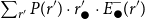 $\sum _{r'} P(r') \cdot r'_{\raise-1pt\hbox{$\bullet$}} \cdot E^{-}_{\raise-1pt\hbox{$\bullet$}}(r')$
that corresponds to
$\sum _{r'} P(r') \cdot r'_{\raise-1pt\hbox{$\bullet$}} \cdot E^{-}_{\raise-1pt\hbox{$\bullet$}}(r')$
that corresponds to
 $r' = ({r}_{\raise-1pt\hbox{$\bullet$}}, {r}_{\ominus }, {r}_{\oplus }, {r}_{\unicode{x25EF}})$
. Since
$r' = ({r}_{\raise-1pt\hbox{$\bullet$}}, {r}_{\ominus }, {r}_{\oplus }, {r}_{\unicode{x25EF}})$
. Since
 $r \mapsto r'$
is a bijection of
$r \mapsto r'$
is a bijection of
 $\mathscr{R}(k) \cap \{r: r_{\raise-1pt\hbox{$\bullet$}}\ge 1\}$
, and
$\mathscr{R}(k) \cap \{r: r_{\raise-1pt\hbox{$\bullet$}}\ge 1\}$
, and
 $r'_{\raise-1pt\hbox{$\bullet$}}= r_{\raise-1pt\hbox{$\bullet$}}$
, and
$r'_{\raise-1pt\hbox{$\bullet$}}= r_{\raise-1pt\hbox{$\bullet$}}$
, and
 $P(r') = P(r)$
we see that
$P(r') = P(r)$
we see that
 \begin{align} \sum _{\substack {r \in {\mathscr R}(k)\\ r_{\raise-1pt\hbox{$\bullet$} \ge 1}}} P(r)\cdot r_{\raise-1pt\hbox{$\bullet$}} \left ({E^{+}_{\raise-1pt\hbox{$\bullet$}}(r) + E^{-}_{\raise-1pt\hbox{$\bullet$}}(r)}\right ) = \sum _{\substack {r \in {\mathscr R}(k)\\ r_{\raise-1pt\hbox{$\bullet$} \ge 1}}} P(r)\cdot r_{\raise-1pt\hbox{$\bullet$}} \left ({E^{+}_{\raise-1pt\hbox{$\bullet$}}(r) + E^{-}_{\raise-1pt\hbox{$\bullet$}}(r')}\right ). \end{align}
Invoking the bounds (7.14) of Claim 7.6, and recalling the definitions of
 $\phi$
,
$\phi$
,
 $E_{\raise-1pt\hbox{$\bullet$}}$
, we upper bound the r.h.s. of (7.25) by
$E_{\raise-1pt\hbox{$\bullet$}}$
, we upper bound the r.h.s. of (7.25) by
 \begin{align} & \sum _{\substack {r \in {\mathscr R}(k)\\ r_{\raise-1pt\hbox{$\bullet$} \ge 1}}} P(r)r_{\raise-1pt\hbox{$\bullet$}} \left (\mathbb{E} \left [ { \int _{{{\boldsymbol{\eta }}}^\wedge _{\raise-1pt\hbox{$\bullet$}, 1, 1}}^{{{\boldsymbol{\eta }}}^\vee _{\raise-1pt\hbox{$\bullet$}, 1, 1}} \unicode {x03C8}_{2^{-r_{\unicode{x25EF}}-r_{\ominus }}} \left (\frac {1+\tanh (w/2)}{2}\right ) \; {\mathrm d} w}\right ]\right.\nonumber\\ & \left.\qquad\qquad\qquad + \mathbb{E}\left [ { \int _{{{\boldsymbol{\eta }}}^\wedge _{\raise-1pt\hbox{$\bullet$}, 1, 1}}^{{{\boldsymbol{\eta }}}^\vee _{\raise-1pt\hbox{$\bullet$}, 1, 1}} \unicode {x03C8}_{2^{-r_{\unicode{x25EF}}-r_{\ominus }}} \left (\frac {1-\tanh (w/2)}{2}\right ) \;{\mathrm d} w }\right ] \right ) = E_{\raise-1pt\hbox{$\bullet$}}. \end{align}
The matchings between the terms for the
 $\oplus , \ominus$
–sums of (7.23), (7.24) are more delicate. In particular, for the
$\oplus , \ominus$
–sums of (7.23), (7.24) are more delicate. In particular, for the
 $\oplus$
–sum it turns out that we can pull off the same trick as above by pairing the term of
$\oplus$
–sum it turns out that we can pull off the same trick as above by pairing the term of
 $\sum _{r} P(r) \cdot r_{\oplus } \cdot E^{+}_{\oplus }(r)$
corresponding to the vector
$\sum _{r} P(r) \cdot r_{\oplus } \cdot E^{+}_{\oplus }(r)$
corresponding to the vector
 $r = ({r}_{\raise-1pt\hbox{$\bullet$}}, {r}_{\oplus }, {r}_{\ominus }, {r}_{\unicode{x25EF}})$
with the term of
$r = ({r}_{\raise-1pt\hbox{$\bullet$}}, {r}_{\oplus }, {r}_{\ominus }, {r}_{\unicode{x25EF}})$
with the term of
 $\sum _{r''} P(r'') \cdot r''_{\oplus } \cdot E^{-}_{\oplus }(r'')$
that corresponds to
$\sum _{r''} P(r'') \cdot r''_{\oplus } \cdot E^{-}_{\oplus }(r'')$
that corresponds to
 $r'' = ({r}_{\raise-1pt\hbox{$\bullet$}}, {r}_{\ominus }+1, {r}_{\oplus }-1, {r}_{\unicode{x25EF}})$
. To see this, note that the mapping
$r'' = ({r}_{\raise-1pt\hbox{$\bullet$}}, {r}_{\ominus }+1, {r}_{\oplus }-1, {r}_{\unicode{x25EF}})$
. To see this, note that the mapping
 $r \mapsto r''$
is a bijection of
$r \mapsto r''$
is a bijection of
 $\mathscr{R}(k) \cap \{r: r_{\oplus }\ge 1\}$
, leaving the quantity
$\mathscr{R}(k) \cap \{r: r_{\oplus }\ge 1\}$
, leaving the quantity
 $P(r)\cdot r_{\oplus }$
invariant as
$P(r)\cdot r_{\oplus }$
invariant as
 \begin{align*} P(r) \cdot{\kern-.5pt} r_{\oplus } & = \frac {(k{\kern-.5pt}-{\kern-1pt}1)!} {{r}_{\raise-1pt\hbox{$\bullet$}}! ({r}_{\oplus }{\kern-.5pt}-{\kern-1pt}1)!{r}_{\ominus }! {r}_{\unicode{x25EF}}!} \cdot p_{\raise-1pt\hbox{$\bullet$}}^{{r}_{\raise-1pt\hbox{$\bullet$}}} p_{\oplus }^{{r}_{\oplus }} p_{\ominus }^{{r}_{\ominus }} p_{\unicode{x25EF}}^{{r}_{\unicode{x25EF}}} = \frac {(k{\kern-.5pt}-{\kern-1pt}1)!} {{r}_{\raise-1pt\hbox{$\bullet$}}! ({r}_{\ominus }{\kern-.5pt}+{\kern-1pt}1)!({r}_{\oplus }-1)! {r}_{\unicode{x25EF}}!} \cdot p_{\raise-1pt\hbox{$\bullet$}}^{{r}_{\raise-1pt\hbox{$\bullet$}}} p_{\oplus }^{{r}_{\oplus }} p_{\ominus }^{{r}_{\ominus }} p_{\unicode{x25EF}}^{{r}_{\unicode{x25EF}}} \cdot (r_{\ominus }{\kern-.5pt}+{\kern-1pt}1)\\& = P(r'') \cdot r''_{\oplus }. \end{align*}
Invoking the bounds (7.15) of Claim 7.6, recalling the definitions of
 $\phi$
,
$\phi$
,
 $E_{\oplus }$
, and arguing as above, we obtain
$E_{\oplus }$
, and arguing as above, we obtain
 \begin{align} \sum _{\substack {r \in {\mathscr R}(k)\\ r_{\oplus }\ge 1}} P(r)\cdot r_{\oplus } \left ({E^{+}_{\oplus }(r) + E^{-}_{\oplus }(r'')}\right ) \le E_{\oplus } . \end{align}
Similarly, using the mapping
 $r\mapsto r'''$
, with
$r\mapsto r'''$
, with
 $r'''\! = (r_{\raise-1pt\hbox{$\bullet$}}, r_{\ominus } - 1, r_{\oplus }+1, r_{\unicode{x25EF}})$
, and following the same steps as above, we get
$r'''\! = (r_{\raise-1pt\hbox{$\bullet$}}, r_{\ominus } - 1, r_{\oplus }+1, r_{\unicode{x25EF}})$
, and following the same steps as above, we get
 \begin{align} \sum _{\substack {r \in {\mathscr R}(k)\\ r_{\ominus }\ge 1}} P(r)\cdot r_{\ominus } \left ({E^{+}_{\ominus }(r) + E^{-}_{\ominus }(r''')}\right ) \le E_{\ominus } . \end{align}
In light of the above, we are now ready to finish the proof of Proposition 2.15.
Proof of Proposition 2.15. Applying Lemma 7.7 on the function
 $\phi$
in the r.h.s. of (7.19) gives
$\phi$
in the r.h.s. of (7.19) gives
 \begin{align} \phi _{2^{-r_{\unicode{x25EF}}-r_{\ominus }}} \left (\frac {1+\tanh (w/2)}{2}\right ) \le \frac {2^{-\boldsymbol{r}_{\ominus }- \boldsymbol{r}_{\unicode{x25EF}}-1}}{1 - 2^{-\boldsymbol{r}_{\ominus }- \boldsymbol{r}_{\unicode{x25EF}}-1}} \le \left (\frac {1}{2}\right )^{\boldsymbol{r}_{\ominus } + \boldsymbol{r}_{\unicode{x25EF}}}. \end{align}
Plugging the above into (7.19) and applying the binomial theorem, further yields
 \begin{align} E_{\raise-1pt\hbox{$\bullet$}} \le (k-1) \cdot p_{\raise-1pt\hbox{$\bullet$}} \left ({1 - \frac {e^{-\frac {d}{2}}}{2}}\right )^{k-2} {\mathbb E}\left [ {|{\boldsymbol{\eta }}_{\raise-1pt\hbox{$\bullet$}, 1,1 }-{\boldsymbol{\eta }}'_{\raise-1pt\hbox{$\bullet$}, 1,1 }|}\right ]. \end{align}
Working in a similar manner, we obtain
 \begin{align} E_{\oplus } & \le (k-1)\cdot p_{\oplus } \left (1-\frac {e^{-\frac {d}{2}}}{2}\right )^{k-2} \!\! {\mathbb E}\left [ {|{\boldsymbol{\eta }}_{\oplus , 1,1 }-{\boldsymbol{\eta }}'_{\oplus , 1,1 }|}\right ] , \quad \text{and}\nonumber\\ E_{\ominus } & \le (k-1)\cdot p_{\ominus } \left (1-\frac {e^{-\frac {d}{2}}}{2}\right )^{k-2} \!\! {\mathbb E}\left [ {|{\boldsymbol{\eta }}_{\ominus , 1,1 }-{\boldsymbol{\eta }}'_{\ominus , 1,1 }|}\right ]. \end{align}
Finally, plugging the bounds (7.30), and (7.31) into (7.22) we see that
 $ W_1(\hat {\rho }_{\oplus },\hat {\rho }'_{\oplus }) + W_1(\hat {\rho }_{\ominus },\hat {\rho }'_{\ominus })$
is upper bounded by
$ W_1(\hat {\rho }_{\oplus },\hat {\rho }'_{\oplus }) + W_1(\hat {\rho }_{\ominus },\hat {\rho }'_{\ominus })$
is upper bounded by
 \begin{align} \frac {d\cdot (k-1)}{2} & \cdot \left (1-\frac {e^{-\frac {d}{2}}}{2}\right )^{k-2} \!\! \Big[ \big(1-e^{-\frac {d}{2}}\big) {\mathbb E}\left [ {|{\boldsymbol{\eta }}_{\raise-1pt\hbox{$\bullet$}, 1,1 }-{\boldsymbol{\eta }}'_{\raise-1pt\hbox{$\bullet$}, 1,1 }|}\right ] + e^{-\frac {d}{2}} {\mathbb E}\left [ {|{\boldsymbol{\eta }}_{\oplus , 1,1 }-{\boldsymbol{\eta }}'_{\oplus , 1,1 }|}\right ] \nonumber \\ & + e^{-\frac {d}{2}} {\mathbb E}\left [ {|{\boldsymbol{\eta }}_{\ominus , 1,1 }-{\boldsymbol{\eta }}'_{\ominus , 1,1 }|}\right ] \Big ]. \end{align}
Recall that we established (7.32) assuming an arbitrary coupling between the coordinates of each pair of distributions
 $(\rho _{\raise-1pt\hbox{$\bullet$}},\rho '_{\raise-1pt\hbox{$\bullet$}})$
,
$(\rho _{\raise-1pt\hbox{$\bullet$}},\rho '_{\raise-1pt\hbox{$\bullet$}})$
,
 $(\rho _{\oplus },\rho '_{\oplus })$
, and
$(\rho _{\oplus },\rho '_{\oplus })$
, and
 $(\rho _{\ominus },\rho '_{\ominus })$
. Therefore, the definition of
$(\rho _{\ominus },\rho '_{\ominus })$
. Therefore, the definition of
 $W_1$
norm and (7.32), imply the first inequality below, while (7.33) follows by the definition (2.22) of
$W_1$
norm and (7.32), imply the first inequality below, while (7.33) follows by the definition (2.22) of
 $\mathrm{dist}_d$
 \begin{align}W_1(\hat\rho_{\oplus},\hat\rho'_{\oplus})+W_1(\hat\rho_{\ominus},\hat\rho'_{\ominus}) & \le\frac{d (k-1)}{2}\left(1-\frac{e^{-\frac{d}{2}}}{2}\right)^{k-2}\left[ \left(1-e^{-\frac{d}{2}}\right) W_1(\rho_{\bullet}, \rho'_{\bullet}) \right.\nonumber\\ & \quad \left.+e^{-\frac{d}{2}} W_1(\rho_{\oplus}, \rho'_{\oplus}) + e^{-\frac{d}{2}}W_1(\rho_{\ominus}, \rho'_{\ominus})\right] \nonumber \\ & \le\frac{d (k-1)}{2}\left(1-\frac{e^{-\frac{d}{2}}}{2}\right)^{k-2}\text{dist}_d(\rho, \rho').\end{align}
Moreover, as per the triangle inequality we see that
 \begin{align} W_1(\hat {\rho }_{\raise-1pt\hbox{$\bullet$}},\hat {\rho }'_{\raise-1pt\hbox{$\bullet$}}) \le W_1(\hat {\rho }_{\oplus },\hat {\rho }'_{\oplus })+ W_1(\hat {\rho }_{\ominus },\hat {\rho }'_{\ominus }) \le \frac {d (k-1)}{2} \left (1-\frac {e^{-\frac {d}{2}}}{2}\right )^{k-2} \mathrm{dist}_d(\rho , \rho '). \end{align}
Plugging the bounds (7.33) and (7.34) into the expression of
 $\mathrm{dist}_{d} \left ({\hat {\rho }, \hat {\rho }'}\right )$
yields
$\mathrm{dist}_{d} \left ({\hat {\rho }, \hat {\rho }'}\right )$
yields
 \begin{align*} \mathrm{dist}_{d} \left ({\hat {\rho }, \hat {\rho }'}\right ) & = (1-e^{-d/2}) \cdot W_1(\hat {\rho }_{\raise-1pt\hbox{$\bullet$}}, \hat {\rho }_{\raise-1pt\hbox{$\bullet$}}') + e^{-d/2} \left ({ W_1(\hat {\rho }_{\oplus }, \hat {\rho }_{\oplus }') + W_1(\hat {\rho }_{\ominus }, \hat {\rho }_{\ominus }')}\right )\\ & \le \frac {d (k-1)}{2} \left (1-\frac {e^{-\frac {d}{2}}}{2}\right )^{k-2} \mathrm{dist}_d(\rho , \rho '). \end{align*}
Recalling the definition of
 ${{{d_{\mathrm{con}}}}}$
, we see that for
${{{d_{\mathrm{con}}}}}$
, we see that for
 $d\lt {{{d_{\mathrm{con}}}}}(k)$
, the operator
$d\lt {{{d_{\mathrm{con}}}}}(k)$
, the operator
 ${\mathrm{LL}}^{\star }_{d,k}$
contracts with respect to the metric
${\mathrm{LL}}^{\star }_{d,k}$
contracts with respect to the metric
 $\mathrm{dist}_{d}$
, as desired.
$\mathrm{dist}_{d}$
, as desired.
7.4 Proof of Proposition 2.13
To get a handle on the
 ${\boldsymbol{\eta }}_{x}^{(\ell )}$
from (2.12), we show that these quantities can be calculated by propagating the extremal boundary condition
${\boldsymbol{\eta }}_{x}^{(\ell )}$
from (2.12), we show that these quantities can be calculated by propagating the extremal boundary condition
 $\boldsymbol{\sigma }^+$
bottom-up toward the root of the tree. Specifically, we consider the operator
$\boldsymbol{\sigma }^+$
bottom-up toward the root of the tree. Specifically, we consider the operator
 \begin{align*} \Lambda ^{+}_{{\mathbb{T}}^{(\ell )}} & \,:\, (\!-\infty ,\infty ]^{V({\mathbb{T}}^{(\ell )})} \to (\!-\infty ,\infty ]^{V({\mathbb{T}}^{(\ell )})}, \quad \eta \mapsto \hat {\eta }=\Lambda ^{+}_{{\mathbb{T}}^{(\ell )}}(\eta ), \end{align*}
defined as follows. For all
 $x\in \partial ^{2\ell }\mathfrak{x}$
we set
$x\in \partial ^{2\ell }\mathfrak{x}$
we set
 $\hat {\eta }_x=\infty$
. Moreover, for a variable
$\hat {\eta }_x=\infty$
. Moreover, for a variable
 $x\in \partial ^{2q}\mathfrak{x}$
with
$x\in \partial ^{2q}\mathfrak{x}$
with
 $q\lt \ell$
having children clauses
$q\lt \ell$
having children clauses
 $a_1,\ldots ,a_t$
, and grandchildren variables
$a_1,\ldots ,a_t$
, and grandchildren variables
 $y_{1,1}, \ldots , y_{1,(k-1)}, \ldots , y_{t,1}, \ldots , y_{t,(k-1)}$
we define
$y_{1,1}, \ldots , y_{1,(k-1)}, \ldots , y_{t,1}, \ldots , y_{t,(k-1)}$
we define
 \begin{align} \hat {\eta }_x & = -\sum _{i=1}^{t} {\boldsymbol{\tau }^+(x)}\mathrm{sign}(x,a_i) \cdot \log \left ( 1- {\Gamma \left ({\boldsymbol{\tau }^+(x)}\mathrm{sign}(x,a_i)\cdot ( \eta _{y_{i,1}}, \ldots , \eta _{y_{1,(k-1)}} ) \right )} \right ). \end{align}
It may not be apparent that the sum above is well-defined as
 $-\infty$
summands may manifest. The following lemma rules out such possibility and shows that the
$-\infty$
summands may manifest. The following lemma rules out such possibility and shows that the
 $\ell$
-fold iteration of
$\ell$
-fold iteration of
 $\Lambda ^{+\, (\ell )}_{{\mathbb{T}}^{(\ell )}}$
, initiated all-
$\Lambda ^{+\, (\ell )}_{{\mathbb{T}}^{(\ell )}}$
, initiated all-
 $(+\infty )$
yields
$(+\infty )$
yields
 ${\boldsymbol{\eta }}^{(\ell )}=({\boldsymbol{\eta }}^{(\ell )}_x)_{x \in V({\mathbb{T}}^{(\ell )})}$
.
${\boldsymbol{\eta }}^{(\ell )}=({\boldsymbol{\eta }}^{(\ell )}_x)_{x \in V({\mathbb{T}}^{(\ell )})}$
.
Lemma 7.9.
The operator
 $\Lambda ^{+}_{{\mathbb{T}}^{(\ell )}}$
is well-defined and
$\Lambda ^{+}_{{\mathbb{T}}^{(\ell )}}$
is well-defined and
 $\Lambda ^{+\, (t)}_{{\mathbb{T}}^{(\ell )}}(+\infty ,\ldots ,+\infty )= {\boldsymbol{\eta }}^{(\ell )}$
for every
$\Lambda ^{+\, (t)}_{{\mathbb{T}}^{(\ell )}}(+\infty ,\ldots ,+\infty )= {\boldsymbol{\eta }}^{(\ell )}$
for every
 $t \ge \ell$
.
$t \ge \ell$
.
Proof. To show that
 $\Lambda ^{+}_{{\mathbb{T}}^{(\ell )}}$
is well defined we verify that, in the notation of (7.35),
$\Lambda ^{+}_{{\mathbb{T}}^{(\ell )}}$
is well defined we verify that, in the notation of (7.35),
 $\hat {\eta }_x\in (\!-\infty ,\infty ]$
for all
$\hat {\eta }_x\in (\!-\infty ,\infty ]$
for all
 $x$
. Indeed, in the expression on the r.h.s. of (7.35) a
$x$
. Indeed, in the expression on the r.h.s. of (7.35) a
 $\pm \infty$
summand can arise only from variables
$\pm \infty$
summand can arise only from variables
 $y_{i,j}$
with
$y_{i,j}$
with
 $\eta _{y_{i,j}}=\infty$
. But the definition of
$\eta _{y_{i,j}}=\infty$
. But the definition of
 $\boldsymbol{\tau }^+$
ensures that such
$\boldsymbol{\tau }^+$
ensures that such
 $y_{i,j}$
either render a zero summand if
$y_{i,j}$
either render a zero summand if
 $\boldsymbol{\tau }^+(x)\mathrm{sign}(x,a_i)=-1$
, or a
$\boldsymbol{\tau }^+(x)\mathrm{sign}(x,a_i)=-1$
, or a
 $+\infty$
summand if
$+\infty$
summand if
 $\boldsymbol{\tau }^+(x)\mathrm{sign}(x,a_i)=1$
. Thus, the sum is well-defined and
$\boldsymbol{\tau }^+(x)\mathrm{sign}(x,a_i)=1$
. Thus, the sum is well-defined and
 $\hat {\eta }_x\in (\!-\infty ,\infty ]$
.
$\hat {\eta }_x\in (\!-\infty ,\infty ]$
.
Further, to verify the identity
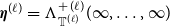 ${\boldsymbol{\eta }}^{(\ell )}=\Lambda ^{+\, (\ell )}_{{\mathbb{T}}^{(\ell )}}(\infty ,\ldots ,\infty )$
, consider a variable
${\boldsymbol{\eta }}^{(\ell )}=\Lambda ^{+\, (\ell )}_{{\mathbb{T}}^{(\ell )}}(\infty ,\ldots ,\infty )$
, consider a variable
 $x$
of
$x$
of
 $\mathbb{T}^{(\ell )}$
. Let
$\mathbb{T}^{(\ell )}$
. Let
 $a_1^+,\ldots ,a_g^+$
be the children (clauses) of
$a_1^+,\ldots ,a_g^+$
be the children (clauses) of
 $x$
with
$x$
with
 $\mathrm{sign}(x,a_i^+)=\boldsymbol{\tau }^+(x)$
. Also let
$\mathrm{sign}(x,a_i^+)=\boldsymbol{\tau }^+(x)$
. Also let
 $y_{11}, \ldots , y_{1(k-1)}, \ldots , y_{g1}, \ldots , y_{g(k-1)}$
be the children of
$y_{11}, \ldots , y_{1(k-1)}, \ldots , y_{g1}, \ldots , y_{g(k-1)}$
be the children of
 $a_1^+,\ldots ,a_g^+$
. Similarly, let
$a_1^+,\ldots ,a_g^+$
. Similarly, let
 $a_1^-,\ldots ,a_h^-$
be the children of
$a_1^-,\ldots ,a_h^-$
be the children of
 $x$
with
$x$
with
 $\mathrm{sign}(x,a_i^-)=-\boldsymbol{\tau }^+(x)$
and let
$\mathrm{sign}(x,a_i^-)=-\boldsymbol{\tau }^+(x)$
and let
 $z_{11},\ldots ,z_{1(k-1)}, \ldots , z_{h1}, \ldots , z_{h(k-1)}$
be their children. Then (7.2), and (7.3) yield
$z_{11},\ldots ,z_{1(k-1)}, \ldots , z_{h1}, \ldots , z_{h(k-1)}$
be their children. Then (7.2), and (7.3) yield
 \begin{align*} {\boldsymbol{\eta }}_x^{(\ell )} & =- \sum _{i=1}^g \log \left (1-\prod _{q=1}^{k-1} \frac {Z\big({\mathbb{T}}_{y_{iq}}^{(\ell )},\boldsymbol{\tau }^+,\boldsymbol{\tau }^+({y_{iq}})\big)} {Z\big({\mathbb{T}}_{y_{iq}}^{(\ell )},\boldsymbol{\tau }^+\big)} \right ) +\sum _{j=1}^h\log \left ( 1- \prod _{q=1}^{k-1} \frac {Z\big({\mathbb{T}}_{z_{jq}}^{(\ell )},\boldsymbol{\tau }^+, -\boldsymbol{\tau }^+({z_{jq}})\big)} {Z\big({\mathbb{T}}_{z_{jq}}^{(\ell )},\boldsymbol{\tau }^+\big)} \right ) \\ & =-\sum _{i=1}^g\log \left (1- \Gamma \left (\mathrm{sign}(x,a_i^+)\boldsymbol{\tau }^+(x)\cdot \left ({\boldsymbol{\eta }}^{(\ell )}_{y_{i1}}, \ldots , {\boldsymbol{\eta }}^{(\ell )}_{y_{i(k-1)}}\right ) \right )\right )\\ & \quad +\sum _{j=1}^h \log \left (1- \Gamma \left ( \mathrm{sign}(x,a_i^-)\boldsymbol{\tau }^+(x)\cdot \left ({\boldsymbol{\eta }}^{(\ell )}_{z_{j1}}, \ldots , {\boldsymbol{\eta }}^{(\ell )}_{z_{j(k-1)}}\right )\right )\right ). \end{align*}
The assertion follows because
 $\mathrm{sign}(x,a_i^+)\boldsymbol{\tau }^+(x)=1$
and
$\mathrm{sign}(x,a_i^+)\boldsymbol{\tau }^+(x)=1$
and
 $\mathrm{sign}(x,a_i^-)\boldsymbol{\tau }^+(x)=-1$
.
$\mathrm{sign}(x,a_i^-)\boldsymbol{\tau }^+(x)=-1$
.
The next aim is to approximate the
 $\ell$
-fold iteration of
$\ell$
-fold iteration of
 $\Lambda ^{+}_{{\mathbb{T}}^{(\ell )}}$
, and more specifically the distribution of
$\Lambda ^{+}_{{\mathbb{T}}^{(\ell )}}$
, and more specifically the distribution of
 ${\boldsymbol{\eta }}_{\mathfrak{x}}^{(\ell )}$
, using a non-random operator. To this end, we need to cope with the
${\boldsymbol{\eta }}_{\mathfrak{x}}^{(\ell )}$
, using a non-random operator. To this end, we need to cope with the
 $\pm \infty$
-entries of the vector
$\pm \infty$
-entries of the vector
 ${\boldsymbol{\eta }}^{(\ell )}$
. This is addressed by Lemma 2.14, proven in Section 7.2, which provides a bound on
${\boldsymbol{\eta }}^{(\ell )}$
. This is addressed by Lemma 2.14, proven in Section 7.2, which provides a bound on
 ${\boldsymbol{\eta }}^{(\ell )}_x$
for variables
${\boldsymbol{\eta }}^{(\ell )}_x$
for variables
 $x$
near the root of the tree.
$x$
near the root of the tree.
In the following we continue to write
 $c$
and
$c$
and
 $(\varepsilon _t)_t$
for the number and the sequence supplied by Lemma 2.14. Guided by Lemma 2.14 we consider the vector
$(\varepsilon _t)_t$
for the number and the sequence supplied by Lemma 2.14. Guided by Lemma 2.14 we consider the vector
 ${\boldsymbol{\eta }}_{\wedge t}^{(\ell )}$
of truncated log-likelihood ratios
${\boldsymbol{\eta }}_{\wedge t}^{(\ell )}$
of truncated log-likelihood ratios
 \begin{align} \left ({\boldsymbol{\eta }}_{\wedge t}^{(\ell )}\right )_x & = \begin{cases}-2t^c & \mbox{ if $x\in \partial ^{2t}\mathfrak{x}$ and } {\boldsymbol{\eta }}_{x}^{(\ell )}\lt -2t^c, \\ 2t^c & \mbox{ if $x\in \partial ^{2t}\mathfrak{x}$ and } {\boldsymbol{\eta }}_{x}^{(\ell )}\gt 2t^c,\\ {\boldsymbol{\eta }}_{x}^{(\ell )} & \mbox{ otherwise}. \end{cases} \end{align}
Further, let
 $ {\boldsymbol{\eta }}^{(\ell ,t)}$
be the result of
$ {\boldsymbol{\eta }}^{(\ell ,t)}$
be the result of
 $t$
iterations of
$t$
iterations of
 $\Lambda ^{+}_{{\mathbb{T}}^{(\ell )}}(\!\cdot \!)$
starting from
$\Lambda ^{+}_{{\mathbb{T}}^{(\ell )}}(\!\cdot \!)$
starting from
 ${\boldsymbol{\eta }}_{\wedge t}^{(\ell )}$
. The following corollary is a direct consequence of Lemma 7.9 and Lemma 2.14.
${\boldsymbol{\eta }}_{\wedge t}^{(\ell )}$
. The following corollary is a direct consequence of Lemma 7.9 and Lemma 2.14.
Corollary 7.10.
For any
 $\ell \gt ct^c$
we have
$\ell \gt ct^c$
we have
 ${\mathbb P}[{\boldsymbol{\eta }}^{(\ell ,t)}_{\mathfrak{x}} \neq {\boldsymbol{\eta }}^{(\ell )}_{\mathfrak{x}}]\lt \varepsilon _t.$
Proof. Due to Lemma 2.14, the truncation in (7.36) is inconsequential with probability at least
 $1-\varepsilon _t$
, in which case
$1-\varepsilon _t$
, in which case
 \begin{align*} {\boldsymbol{\eta }}^{(\ell ,t)} = \Lambda ^{+\, (t)}_{{\mathbb{T}}^{(\ell )}}\left ({\boldsymbol{\eta }}_{\wedge t}^{(\ell )}\right ) = \Lambda ^{+\, (t)}_{{\mathbb{T}}^{(\ell )}}({\boldsymbol{\eta }}^{(\ell )}) = \Lambda ^{+\, (\ell + t)}_{{\mathbb{T}}^{(\ell )}}(+\infty , \ldots , +\infty ) = {\boldsymbol{\eta }}^{(\ell )}, \end{align*}
where the last equality follows from Lemma 7.9.
Recall that we defined the non-random operator
 ${\mathrm{LL}}^{\star }_{d,k}$
from (2.17), mimicking
${\mathrm{LL}}^{\star }_{d,k}$
from (2.17), mimicking
 $\Lambda ^{+}_{{\mathbb{T}}^{(\ell )}}$
. To make the connection between the random operator
$\Lambda ^{+}_{{\mathbb{T}}^{(\ell )}}$
. To make the connection between the random operator
 $\Lambda ^{+}_{{\mathbb{T}}^{(\ell )}}$
and
$\Lambda ^{+}_{{\mathbb{T}}^{(\ell )}}$
and
 ${\mathrm{LL}}^{\star }_{d,k}$
precise, we introduce the following concepts. Given a tree formula
${\mathrm{LL}}^{\star }_{d,k}$
precise, we introduce the following concepts. Given a tree formula
 $T$
we write
$T$
we write
 $V_{\raise-1pt\hbox{$\bullet$}}(T)$
, for the set of
$V_{\raise-1pt\hbox{$\bullet$}}(T)$
, for the set of
 $x$
variables of
$x$
variables of
 $T$
that appear both as positive and negative literals in the sub-tree
$T$
that appear both as positive and negative literals in the sub-tree
 $T_x$
comprising
$T_x$
comprising
 $x$
and its the progeny. We define
$x$
and its the progeny. We define
 $V_{\unicode{x25EF}}(T), V_{\oplus }(T)$
, and
$V_{\unicode{x25EF}}(T), V_{\oplus }(T)$
, and
 $V_{\ominus }(T)$
similarly. Note that the above sets constitute a partition of
$V_{\ominus }(T)$
similarly. Note that the above sets constitute a partition of
 $V(T)$
. We use
$V(T)$
. We use
 $\textrm {tp}: V(T) \to \{\raise-1pt\hbox{$\bullet$}, \oplus , \ominus , \mathrel {{\Large\unicode{x25EF}}}\}$
to indicate the part each vertex belongs to. We denote with
$\textrm {tp}: V(T) \to \{\raise-1pt\hbox{$\bullet$}, \oplus , \ominus , \mathrel {{\Large\unicode{x25EF}}}\}$
to indicate the part each vertex belongs to. We denote with
 $\mathbb{T}^{(\ell )}_{\raise-1pt\hbox{$\bullet$}}$
the random Galton-Watson formula
$\mathbb{T}^{(\ell )}_{\raise-1pt\hbox{$\bullet$}}$
the random Galton-Watson formula
 $\mathbb{T}$
conditioned on the root satisfying
$\mathbb{T}$
conditioned on the root satisfying
 $\textrm {tp}(\mathfrak{x}) = \raise-1pt\hbox{$\bullet$}$
. We define
$\textrm {tp}(\mathfrak{x}) = \raise-1pt\hbox{$\bullet$}$
. We define
 $\mathbb{T}^{(\ell )}_{\oplus }$
, and
$\mathbb{T}^{(\ell )}_{\oplus }$
, and
 $\mathbb{T}^{(\ell )}_{\ominus }$
analogously. Degenerately, we also write
$\mathbb{T}^{(\ell )}_{\ominus }$
analogously. Degenerately, we also write
 $\mathbb{T}^{(\ell )}_{\unicode{x25EF}}$
for the formula comprised by a single variable
$\mathbb{T}^{(\ell )}_{\unicode{x25EF}}$
for the formula comprised by a single variable
 $\mathfrak{x}$
. Let us denote with
$\mathfrak{x}$
. Let us denote with
 $\hat {\eta }_{\raise-1pt\hbox{$\bullet$}}^{(\ell ,t)}$
the distribution of
$\hat {\eta }_{\raise-1pt\hbox{$\bullet$}}^{(\ell ,t)}$
the distribution of
 $({\boldsymbol{\eta }}_{\wedge t}^{(\ell )})_{\mathfrak{x}}$
in
$({\boldsymbol{\eta }}_{\wedge t}^{(\ell )})_{\mathfrak{x}}$
in
 $\mathbb{T}^{(\ell )}_{\raise-1pt\hbox{$\bullet$}}$
. Moreover, let
$\mathbb{T}^{(\ell )}_{\raise-1pt\hbox{$\bullet$}}$
. Moreover, let
 $\bar {\eta }^{(\ell -t)}_{\raise-1pt\hbox{$\bullet$}}$
be the distribution of
$\bar {\eta }^{(\ell -t)}_{\raise-1pt\hbox{$\bullet$}}$
be the distribution of
 \begin{align*} {\boldsymbol{\eta }}_{\mathfrak{x}}^{(\ell -t)} \cdot \unicode {x1D7D9}\left \{|{\boldsymbol{\eta }}_{\mathfrak{x}}^{(\ell -t)}| \le 2t^c\right \} + 2t^c \cdot \unicode {x1D7D9}\left \{{\boldsymbol{\eta }}_{\mathfrak{x}}^{(\ell -t)} \gt 2t^c\right \} -2t^c \cdot \unicode {x1D7D9}\left \{{\boldsymbol{\eta }}_{\mathfrak{x}}^{(\ell -t)} \lt -2t^c\right \}, \end{align*}
i.e., the truncation of
 ${\boldsymbol{\eta }}_{\mathfrak{x}}^{(\ell -t)}$
in
${\boldsymbol{\eta }}_{\mathfrak{x}}^{(\ell -t)}$
in
 $\mathbb{T}^{(\ell )}_{\raise-1pt\hbox{$\bullet$}}$
. Analogously we define the distributions
$\mathbb{T}^{(\ell )}_{\raise-1pt\hbox{$\bullet$}}$
. Analogously we define the distributions
 $ \hat {\eta }^{(\ell , t)}_{\oplus }, \hat {\eta }^{(\ell , t)}_{\ominus }$
, and
$ \hat {\eta }^{(\ell , t)}_{\oplus }, \hat {\eta }^{(\ell , t)}_{\ominus }$
, and
 $\bar {\eta }^{(\ell -t)}_{\oplus }, \bar {\eta }^{(\ell - t)}_{\ominus }$
. Notice that, degenerately,
$\bar {\eta }^{(\ell -t)}_{\oplus }, \bar {\eta }^{(\ell - t)}_{\ominus }$
. Notice that, degenerately,
 $\hat {\eta }^{(\ell ,t)}_{\unicode{x25EF}} = \bar {\eta }^{(\ell -t)}_{\unicode{x25EF}} = \delta _{0}$
.
$\hat {\eta }^{(\ell ,t)}_{\unicode{x25EF}} = \bar {\eta }^{(\ell -t)}_{\unicode{x25EF}} = \delta _{0}$
.
Lemma 7.11.
For
 $\ell \gt ct^c$
we have that
$\ell \gt ct^c$
we have that
 $ \left (\hat {\eta }^{(\ell , t)}_{\raise-1pt\hbox{$\bullet$}}, \hat {\eta }^{(\ell , t)}_{\oplus }, \hat {\eta }^{(\ell , t)}_{\ominus }\right ) = {\mathrm{LL}}^{\star }_{d,k} \left (\bar {\eta }^{(\ell - t)}_{\raise-1pt\hbox{$\bullet$}}, \bar {\eta }^{(\ell - t)}_{\oplus }, \bar {\eta }^{(\ell - t)}_{\ominus }\right ).$
Proof. We use induction on
 $t$
. Specifically, let
$t$
. Specifically, let
 $\nu = \left (\nu _{\raise-1pt\hbox{$\bullet$}}, \nu _{\oplus }, \nu _{\ominus }\right )$
be any triplet in
$\nu = \left (\nu _{\raise-1pt\hbox{$\bullet$}}, \nu _{\oplus }, \nu _{\ominus }\right )$
be any triplet in
 $\mathscr{P}(\!-\infty , \infty ] \times \mathscr{P}[0, +\infty ] \times \mathscr{P}[-\infty ,0]$
, and
$\mathscr{P}(\!-\infty , \infty ] \times \mathscr{P}[0, +\infty ] \times \mathscr{P}[-\infty ,0]$
, and
 $\nu ^{(t)} ={\mathrm{LL}}^{\star (t)}_{d,k}(\nu )$
be the outcome of the
$\nu ^{(t)} ={\mathrm{LL}}^{\star (t)}_{d,k}(\nu )$
be the outcome of the
 $t$
-fold application of
$t$
-fold application of
 ${\mathrm{LL}}^{\star }_{d,k}$
. Moreover, let
${\mathrm{LL}}^{\star }_{d,k}$
. Moreover, let
 $({\boldsymbol{\eta }}_x)_{x\in V(\mathbb{T}^{(t)})}$
be a vector of independent samples with
$({\boldsymbol{\eta }}_x)_{x\in V(\mathbb{T}^{(t)})}$
be a vector of independent samples with
 ${\boldsymbol{\eta }}_x \sim \nu _{\textrm {tp}(x)}$
. We claim that root value
${\boldsymbol{\eta }}_x \sim \nu _{\textrm {tp}(x)}$
. We claim that root value
 ${\boldsymbol{\eta }}^{(t)}_{\mathfrak{x}}$
of the random operator
${\boldsymbol{\eta }}^{(t)}_{\mathfrak{x}}$
of the random operator
 $\Lambda ^{+\, (t)}_{{\mathbb{T}^{(t)}}}$
, coincides with
$\Lambda ^{+\, (t)}_{{\mathbb{T}^{(t)}}}$
, coincides with
 $\nu _{\textrm {tp}(\mathfrak{x})}$
. Indeed, for
$\nu _{\textrm {tp}(\mathfrak{x})}$
. Indeed, for
 $t=1$
the claim follows readily from the definitions. For the inductive step, we notice that the
$t=1$
the claim follows readily from the definitions. For the inductive step, we notice that the
 $t$
-fold application of
$t$
-fold application of
 ${\mathrm{LL}}^{\star }_{d,k}$
is obtained by applying
${\mathrm{LL}}^{\star }_{d,k}$
is obtained by applying
 ${\mathrm{LL}}^{\star }_{d,k}$
to the
${\mathrm{LL}}^{\star }_{d,k}$
to the
 $(t-1)$
-fold application. Per the induction hypothesis
$(t-1)$
-fold application. Per the induction hypothesis
 \begin{align} \left ({\Lambda ^{+\, (t-1)}_{\mathbb{T}^{(t-1)}}({\boldsymbol{\eta }}_x)_{x}}\right )_{\mathfrak{x}} \sim \nu ^{(t-1)}_{\textrm {tp}(\mathfrak{x})}. \end{align}
Applying
 ${\mathrm{LL}}^{\star }_{d,k}$
to
${\mathrm{LL}}^{\star }_{d,k}$
to
 $\nu ^{(t-1)}$
implies the result as the first layer of
$\nu ^{(t-1)}$
implies the result as the first layer of
 $\mathbb{T}^{(t)}$
is independent of the subtrees rooted at the grandchildren
$\mathbb{T}^{(t)}$
is independent of the subtrees rooted at the grandchildren
 $\partial ^2 \mathfrak{x}$
of the root, which are distributed as i.i.d. copies of
$\partial ^2 \mathfrak{x}$
of the root, which are distributed as i.i.d. copies of
 $\mathbb{T}^{(t-1)}$
. The lemma follows from applying the above identity to
$\mathbb{T}^{(t-1)}$
. The lemma follows from applying the above identity to
 $\nu = \left (\bar {\eta }^{(\ell - t)}_{\raise-1pt\hbox{$\bullet$}}, \bar {\eta }^{(\ell - t)}_{\oplus }, \bar {\eta }^{(\ell - t)}_{\ominus }\right )$
.
$\nu = \left (\bar {\eta }^{(\ell - t)}_{\raise-1pt\hbox{$\bullet$}}, \bar {\eta }^{(\ell - t)}_{\oplus }, \bar {\eta }^{(\ell - t)}_{\ominus }\right )$
.
Refining the definition of the
 $\mathrm{BP}_{d,k}$
operator in (1.3), we write
$\mathrm{BP}_{d,k}$
operator in (1.3), we write
 $\mathrm{BP}_{d,k}^{\raise-1pt\hbox{$\bullet$}}$
for the operator obtained from
$\mathrm{BP}_{d,k}^{\raise-1pt\hbox{$\bullet$}}$
for the operator obtained from
 $\mathrm{BP}_{d,k}$
upon conditioning on
$\mathrm{BP}_{d,k}$
upon conditioning on
 $\boldsymbol{d}^+,\boldsymbol{d}^- \ge 1$
. Similarly
$\boldsymbol{d}^+,\boldsymbol{d}^- \ge 1$
. Similarly
 $\mathrm{BP}_{d,k}^{\oplus }$
and
$\mathrm{BP}_{d,k}^{\oplus }$
and
 $\mathrm{BP}_{d,k}^{\ominus }$
are obtained from
$\mathrm{BP}_{d,k}^{\ominus }$
are obtained from
 $\mathrm{BP}_{d,k}$
upon conditioning on
$\mathrm{BP}_{d,k}$
upon conditioning on
 $\boldsymbol{d}^+\ge 1,\boldsymbol{d}^- = 0$
, and
$\boldsymbol{d}^+\ge 1,\boldsymbol{d}^- = 0$
, and
 $\boldsymbol{d}^+ = 0 ,\boldsymbol{d}^- \ge 1$
, respectively. We define
$\boldsymbol{d}^+ = 0 ,\boldsymbol{d}^- \ge 1$
, respectively. We define
 \begin{align*} \pi ^{\raise-1pt\hbox{$\bullet$}}_{d,k}=\mathrm{BP}_{d,k}^{\raise-1pt\hbox{$\bullet$}} \left (\pi _{d,k}\right ), \pi ^{\oplus }_{d,k}=\mathrm{BP}_{d,k}^{\oplus } \left (\pi _{d,k}\right ), \pi ^{\ominus }_{d,k}=\mathrm{BP}_{d,k}^{\ominus } \left (\pi _{d,k}\right ) . \end{align*}
Let us write
 ${\gamma }, {\gamma ^{-1}}$
for the continuous and mutually inverse real functions
${\gamma }, {\gamma ^{-1}}$
for the continuous and mutually inverse real functions
 \begin{align} {\gamma }\,:\, \mathbb{R} \to (0,1),z \mapsto (1 + \tanh (z/2))/2, & & {\gamma ^{-1}}\,:\, (0,1) \to \mathbb{R},p \mapsto \log (p/(1-p)). \end{align}
Let
 $\rho ^{\raise-1pt\hbox{$\bullet$}}_{d,k}={\gamma ^{-1}}(\pi _{d,k}^{\raise-1pt\hbox{$\bullet$}})$
, and define
$\rho ^{\raise-1pt\hbox{$\bullet$}}_{d,k}={\gamma ^{-1}}(\pi _{d,k}^{\raise-1pt\hbox{$\bullet$}})$
, and define
 $\rho ^{\oplus }_{d,k}, \rho ^{\ominus }_{d,k}$
similarly.
$\rho ^{\oplus }_{d,k}, \rho ^{\ominus }_{d,k}$
similarly.
Claim 7.12.
The vector
 $({\rho ^{\raise-1pt\hbox{$\bullet$}}_{d,k}, \rho ^{\oplus }_{d,k}, \rho ^{\ominus }_{d,k}} )$
is a fixed point of the operator
$({\rho ^{\raise-1pt\hbox{$\bullet$}}_{d,k}, \rho ^{\oplus }_{d,k}, \rho ^{\ominus }_{d,k}} )$
is a fixed point of the operator
 ${\mathrm{LL}}^{\star }_{d,k}$
.
${\mathrm{LL}}^{\star }_{d,k}$
.
Proof. Let
 $\rho _{d,k}={\gamma ^{-1}}\bigl (\pi _{d,k}\bigr )$
. First, we claim that
$\rho _{d,k}={\gamma ^{-1}}\bigl (\pi _{d,k}\bigr )$
. First, we claim that
 \begin{align} {\mathrm{LL}}^{\star }_{d,k}\left ({\rho _{d,k}, \rho _{d,k}, \rho _{d,k}}\right ) = \left ({\rho ^{\raise-1pt\hbox{$\bullet$}}_{d,k}, \rho ^{\oplus }_{d,k}, \rho ^{\ominus }_{d,k}}\right ). \end{align}
Indeed, since all input distributions are the same, by Proposition 2.1, the two summands in the left term of (2.21) corresponding to
 $\boldsymbol{d}_{+}^{\star }$
and
$\boldsymbol{d}_{+}^{\star }$
and
 $\boldsymbol{d}_{-}^{\star }$
are identically distributed, and also identically distributed to the sums that appear in the other two terms. Therefore, (7.39) follows directly from the definitions of
$\boldsymbol{d}_{-}^{\star }$
are identically distributed, and also identically distributed to the sums that appear in the other two terms. Therefore, (7.39) follows directly from the definitions of
 $\mathrm{BP}_{d,k}^{\raise-1pt\hbox{$\bullet$}}, \mathrm{BP}_{d,k}^{\oplus }$
, and
$\mathrm{BP}_{d,k}^{\raise-1pt\hbox{$\bullet$}}, \mathrm{BP}_{d,k}^{\oplus }$
, and
 $ \mathrm{BP}_{d,k}^{\ominus }$
. The claim now follows from (7.39), the definition of the operator
$ \mathrm{BP}_{d,k}^{\ominus }$
. The claim now follows from (7.39), the definition of the operator
 ${\mathrm{LL}}^{\star }_{d,k}$
, and the law of total probability.
${\mathrm{LL}}^{\star }_{d,k}$
, and the law of total probability.
Let
 $\rho ^{(\ell )}$
be the distribution of the log-likelihood ratio
$\rho ^{(\ell )}$
be the distribution of the log-likelihood ratio
 ${\boldsymbol{\eta }}^{(\ell )}_{\mathfrak{x}}$
.
${\boldsymbol{\eta }}^{(\ell )}_{\mathfrak{x}}$
.
Corollary 7.13.
For
 $d \lt {{{d_{\mathrm{con}}}}}(k)$
the sequence
$d \lt {{{d_{\mathrm{con}}}}}(k)$
the sequence
 $\left ({{\gamma }\left ({\rho ^{(\ell )}}\right )}\right )_{\ell }$
converges weakly to
$\left ({{\gamma }\left ({\rho ^{(\ell )}}\right )}\right )_{\ell }$
converges weakly to
 $\pi _{d,k}$
.
$\pi _{d,k}$
.
Proof. The result follows by combining Corollary 7.10, Lemma 7.11, Proposition 2.15, Claim 7.12, and applying the continuous mapping theorem and the law of total probability.
Proof of Proposition 2.13. Recall that we write
 $\Lambda _{\mathbb{T}^{(\ell )}}^{+ \, (\ell )}$
for the
$\Lambda _{\mathbb{T}^{(\ell )}}^{+ \, (\ell )}$
for the
 $\ell$
-fold iteration of the operator
$\ell$
-fold iteration of the operator
 $\Lambda ^{+}_{{\mathbb{T}}}$
. Let us write
$\Lambda ^{+}_{{\mathbb{T}}}$
. Let us write
 $\boldsymbol{\theta }^{(\ell )}_{\mathfrak{x}} = \bigl (\Lambda ^{+\, (\ell )}_{\mathbb{T}^{(\ell )}}(0, \ldots , 0)\bigr )_{\mathfrak{x}}$
. Using arguments similar to Fact 4.2, we can show that
$\boldsymbol{\theta }^{(\ell )}_{\mathfrak{x}} = \bigl (\Lambda ^{+\, (\ell )}_{\mathbb{T}^{(\ell )}}(0, \ldots , 0)\bigr )_{\mathfrak{x}}$
. Using arguments similar to Fact 4.2, we can show that
 $\boldsymbol{\theta }^{(\ell )}_{\mathfrak{x}}$
is nothing but the distribution of the random variable
$\boldsymbol{\theta }^{(\ell )}_{\mathfrak{x}}$
is nothing but the distribution of the random variable
 ${\gamma ^{-1}}({\mathbb P}\left [ {\boldsymbol{\tau }^{(\ell )}(\mathfrak{x})=1\mid \mathbb{T}}\right ] )$
. Therefore,
${\gamma ^{-1}}({\mathbb P}\left [ {\boldsymbol{\tau }^{(\ell )}(\mathfrak{x})=1\mid \mathbb{T}}\right ] )$
. Therefore,
 \begin{align*} {{\mathbb P}[\boldsymbol{\tau }^{(\ell )}(\mathfrak{x})=1\mid \mathbb{T}]}\sim {\gamma }(\boldsymbol{\theta }^{(\ell )}_{\mathfrak{x}}), & & \text{ and } & & {{\mathbb P}[\boldsymbol{\tau }^{(\ell )}(\mathfrak{x})=1 \mid \forall y\in \partial ^{2\ell }\mathfrak{x}: \boldsymbol{\tau }^{(\ell )}(y) = \boldsymbol{\tau }^+(y),\mathbb{T}]} \sim {\gamma }({\boldsymbol{\eta }}^{(\ell )}_{\mathfrak{x}}). \end{align*}
Due to Lemma 2.12,
 $0 \le {\gamma }(\boldsymbol{\theta }^{(\ell )}_{\mathfrak{x}}) \le {\gamma }({\boldsymbol{\eta }}^{(\ell )}_{\mathfrak{x}}) \le 1$
. Moreover, from Lemma 7.11, Proposition 2.15, and Claim 7.12, we see that for
$0 \le {\gamma }(\boldsymbol{\theta }^{(\ell )}_{\mathfrak{x}}) \le {\gamma }({\boldsymbol{\eta }}^{(\ell )}_{\mathfrak{x}}) \le 1$
. Moreover, from Lemma 7.11, Proposition 2.15, and Claim 7.12, we see that for
 $d \lt {{{d_{\mathrm{con}}}}}(k)$
the sequence
$d \lt {{{d_{\mathrm{con}}}}}(k)$
the sequence
 $\bigl ({\gamma }(\boldsymbol{\theta }^{(\ell )}_{\mathfrak{x}})\bigr )_\ell$
converges weakly to
$\bigl ({\gamma }(\boldsymbol{\theta }^{(\ell )}_{\mathfrak{x}})\bigr )_\ell$
converges weakly to
 $\pi _{d,k}$
. Finally, Corollary 7.13 implies that
$\pi _{d,k}$
. Finally, Corollary 7.13 implies that
 $\bigl ({\gamma }({\boldsymbol{\eta }}^{(\ell )}_{\mathfrak{x}})\bigr )_\ell$
also converges weakly to
$\bigl ({\gamma }({\boldsymbol{\eta }}^{(\ell )}_{\mathfrak{x}})\bigr )_\ell$
also converges weakly to
 $\pi _{d,k}$
, and thus,
$\pi _{d,k}$
, and thus,
 \begin{align*} \lim _{\ell \to \infty } \mathbb{E} \left |{\gamma }\big(\boldsymbol{\theta }^{(\ell )}_{\mathfrak{x}}\big)- {\gamma }\big({\boldsymbol{\eta }}^{(\ell )}_{\mathfrak{x}}\big)\right | = \lim _{\ell \to \infty } \left |\mathbb{E}\left [ {{\gamma }\big(\boldsymbol{\theta }^{(\ell )}_{\mathfrak{x}}\big)}\right ] - \mathbb{E}\left [ {{\gamma }\big({\boldsymbol{\eta }}^{(\ell )}_{\mathfrak{x}}\big)}\right ] \right | = 0, \end{align*}
implying the assertion.
Acknowledgements
We would like to thank the anonymous referees for thoroughly reviewing our paper and for suggesting valuable corrections and improvements.
Amin Coja-Oghlan is supported by DFG CO 646/3, DFG CO 646/5 and DFG CO 646/6. Catherine Greenhill is supported by ARC DP250101611. Vincent Pfenninger is supported by the Austrian Science Fund (FWF) [10.55776 / 16502]. Pavel Zakharov is supported by DFG CO 646/6. Kostas Zampetakis is supported by DFG CO 646/5. For open access, the authors have applied a CC BY public copyright licence to any Author Accepted Manuscript version arising from this submission.


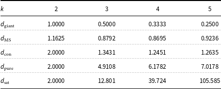


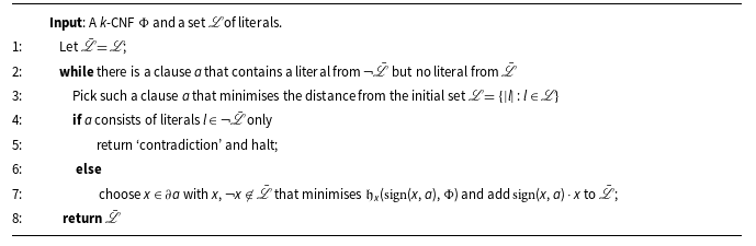


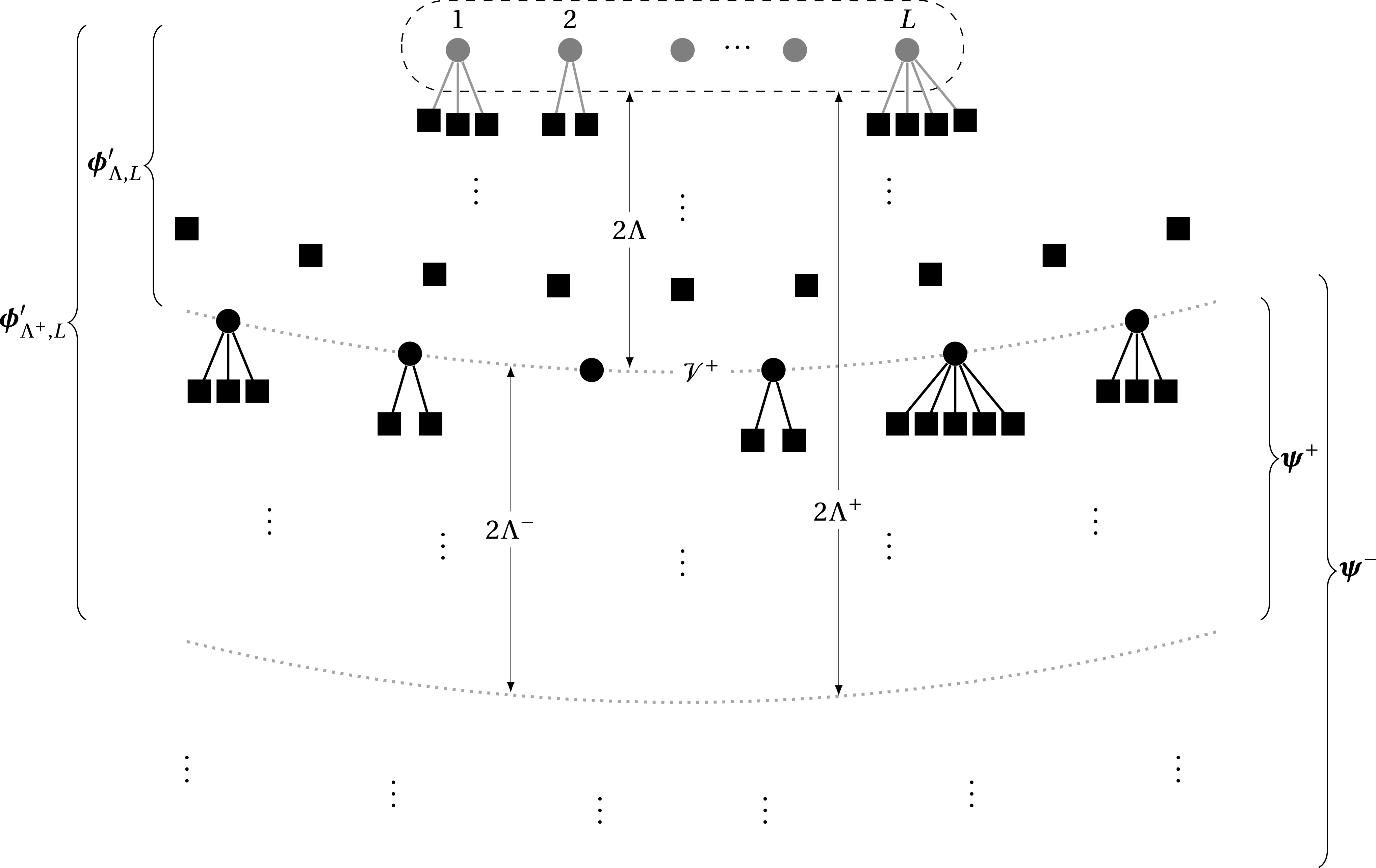


 Open access