


1. Introduction
Inspired by the olfactory system of animals, the technological concept of electronic noses (E-noses) has gained extensive application in odor studies such as odor-source localization [Reference Chen and Huang1], plume tracking [Reference Ishida, Nakamoto, Moriizumi, Kikas and Janata2], and gas distribution mapping [Reference Monroy, Blanco and Gonzalez-Jimenez3] using robots with sensor arrays [Reference Wilson4]. Odor classification in both grounded and mobile robotic systems is a common focus in the field of e-nose applications [Reference Moshayedi, Khan, Shuxin, Kuan, Jiandong, Soleimani and Razi5–Reference Monroy, Ruiz-Sarmiento, Moreno, Galindo and Gonzalez-Jimenez7]. The grounded systems use a three-phase sampling process: first, exposing the sensor array to a reference gas, then to a target gas for a set period, and finally, analyzing the results based on the steady-state response of the sensors [Reference Trincavelli, Coradeschi and Loutfi8]. A similar approach is used on mobile robots, which requires the robots to stop each time an odor sample is to be collected [Reference Reddy, Murthy and Vergassola9]. Applications that require continuous measurement of the environment at different locations, such as pollution monitoring or leak detection, benefit more from mobile robot classification [Reference Marques, Martins and de Almeida10, Reference Soldan, Bonow and Kroll11].
The developed robot base incorporates a vertically mounted $20$
cm motorized bioconical spool system (far right). The spool is driven by a Faulhaber brushless DC motor (
$20$
cm motorized bioconical spool system (far right). The spool is driven by a Faulhaber brushless DC motor ( $11$
cm length), whose shaft interfaces with a
$11$
cm length), whose shaft interfaces with a $4$
cm outer-diameter coupling on one end and an
$4$
cm outer-diameter coupling on one end and an $0.8$
cm D-profile shaft on the other. The shaft is supported by a sleeve bearing, ensuring smooth rotation under low shaft displacement. The spool assembly is enclosed within the base chamber and constrained between two structural plates: an upper mounting plate that supports the motor and provides space for the motor driver, and a lower plate with a roller bearing to minimize rotational resistance (middle block). The chamber is sealed with end caps to prevent air leakage. The complete base structure stands
$0.8$
cm D-profile shaft on the other. The shaft is supported by a sleeve bearing, ensuring smooth rotation under low shaft displacement. The spool assembly is enclosed within the base chamber and constrained between two structural plates: an upper mounting plate that supports the motor and provides space for the motor driver, and a lower plate with a roller bearing to minimize rotational resistance (middle block). The chamber is sealed with end caps to prevent air leakage. The complete base structure stands $34$
cm tall. A frontal platform accommodates four directional actuators (red dashed region), and a mid-height outlet of
$34$
cm tall. A frontal platform accommodates four directional actuators (red dashed region), and a mid-height outlet of $8.5$
cm in outer diameter and
$8.5$
cm in outer diameter and $8$
cm long guides the everted robot body. This geometry positions the inflated body approximately
$8$
cm long guides the everted robot body. This geometry positions the inflated body approximately $15.5$
cm above ground level during eversion.
$15.5$
cm above ground level during eversion.

However, most odor classification studies with traditional robots are conducted in structured or constrained environments with relatively large workspaces, and mobile robots require several actuators to move and extend their degrees of freedom [Reference Steele, Han, Karki, Al-Wahedi, Ayoade, Sweatt, Albert and Yearsley12]. Some limitations of the traditional mobile robots have been compensated through extensive design approaches, including navigation through artificial vision and chemical sensing [Reference Monroy, Ruiz-Sarmiento, Moreno, Melendez-Fernandez, Galindo and Gonzalez-Jimenez13–Reference de Croon, O’connor, Nicol and Izzo15], swarm intelligence algorithms to improve motion efficiency [Reference Wang, Lin, Liu and Fu16], open sampling systems [Reference Monroy, Ruiz-Sarmiento, Moreno, Galindo and Gonzalez-Jimenez7, Reference Fan, Schaffernicht and Lilienthal17, Reference Voss, Mendes Júnior, Farinelli and Stevan18], and localization via adaptive bio-inspired navigation using fuzzy inference methods [Reference Wang and Pang19]. Furthermore, in a quest to improve the flexibility and maneuverability of these robots, recent studies have explored bio-inspired soft robots, such as worm-inspired robots for pipe inspection [Reference Bennetts, Lilienthal, Neumann and Trincavelli20–Reference Liu, Song, Fang, Zhao and Cao23]. However, these robots suffer from a notable drawback in pipe exploration and even open space, particularly the amount of energy used to propel themselves against the pipe walls, which also generates unwanted vibrations and friction in the system [Reference Zhao, Zhang and Wang24].
A more promising alternative to address these challenges is another bio-inspired class of soft robots known as vine or soft-growing robots (SGRs) [Reference Coad, Blumenschein, Cutler, Zepeda, Naclerio, El-Hussieny, Mehmood, Ryu, Hawkes and Okamura25]. These robots are air-driven and mimic the growth behavior of vine plants. Constructed from low-density polyethylene (LDPE) or fabric, they are built into inverted tubes and wound on a motorized spool within a pressurized chamber or base station (Figure 1). Growth is achieved by applying compressed air at the inverted tip as the spool unwinds the LDPE material [Reference Blumenschein, Coad, Haggerty, Okamura and Hawkes26]. Due to advancements in modeling [Reference El-Hussieny, Hameed and Zaky27, Reference Yu, Liu, Zhao, Hou, Hong and Zhang28], task planning [Reference Stroppa29, Reference Exarchos, Wang, Do, Stroppa, Coad, Okamura and Liu30], tool attachment techniques [Reference Girerd, Alvarez, Hawkes and Morimoto31, Reference Jeong, Coad, Blumenschein, Luo, Mehmood, Kim, Okamura and Ryu32], and actuation/steering techniques [Reference Do, Wu, Zhao and Okamura33–Reference Dezaki, Bodaghi, Serjouei, Afazov and Zolfagharian35], these robots possess the potential for multi-degrees of freedom and maneuverability. They can grow and retract (i.e., evert) over long distances through passive environments [Reference Greer, Blumenschein, Alterovitz, Hawkes and Okamura36] or teleoperated steering [Reference Stroppa, Luo, Yoshida, Coad, Blumenschein and Okamura37, Reference Stroppa, Selvaggio, Agharese, Luo, Blumenschein, Hawkes and Okamura38] while carrying tools such as cameras or sensors [Reference Jeong, Coad, Blumenschein, Luo, Mehmood, Kim, Okamura and Ryu32]. Their performance has also been improved recently through machine-learning (ML) techniques, with work on reinforcement learning for obstacle-aware navigation [Reference El-Hussieny and Hameed39, Reference Ataka and Sandiwan40] or other methodologies for sensing and control enhancement [Reference Huang, Li, Zhang, Wang, Zhou and Li41–Reference Kalibala, Nada, Ishii and El-Hussieny43].
In this study, we introduce the concept of olfactory soft growing robot (oSGR) for gas detection and classification tasks. As illustrated in Figure 2, the proposed system consists of a pneumatically actuated SGR equipped with a tip-mount device. This tip mount facilitates olfactory sensing by housing an electronic nose (comprising four metal–oxide gas sensors: TGS2600, TGS2602, TGS2611, and TGS2620) together with a passive aspirator. We present the modeling, design, and characterization of the tip-mount device under various eversion and bending configurations. Additionally, we demonstrate the capabilities of the olfactory SGR through data collection in two scenarios: (i) in-transit and static sampling, where data were recorded over $60$
seconds at three distances –
$60$
seconds at three distances – $20$
cm,
$20$
cm, $40$
cm, and
$40$
cm, and $80$
cm – following brief motions of
$80$
cm – following brief motions of $10$
s,
$10$
s, $20$
s, and
$20$
s, and $40$
s, respectively, conducted at a constant approach speed of
$40$
s, respectively, conducted at a constant approach speed of $2$
cm/s; and (ii) dynamic sampling, in which the robot continuously advanced toward the odor source along a
$2$
cm/s; and (ii) dynamic sampling, in which the robot continuously advanced toward the odor source along a $100$
cm path at speeds of
$100$
cm path at speeds of $5$
cm/s and
$5$
cm/s and $10$
cm/s.
$10$
cm/s.
The sensor data were subsequently preprocessed and used to train and evaluate twelve different classification models to assess the feasibility of our proposed robot for autonomous odor classification. Our experiments demonstrate successful eversion of the robot with the tip mount and reliable olfactory sensing through the passive aspirator. Additionally, results from the ML classification indicate that the raw olfactory data collected during the robot’s motion are inherently separable across different odor classes, even under varying source proximities and approach velocities.
The contributions and scope of this work are as follows:
-
i. Design and implementation of a pneumatically driven SGR capable of everting through confined environments while lifting a tip-mounted device without physical contact;
-
ii. Modeling, development, and characterization of a compact, motorized tip-mounted mechanism for transporting multiple sensors on-board without hindering the growth or flexibility of the SGR; and
-
iii. oSGR enabled the collection of static and dynamic cross-sensitivity olfactory data, integrated into an ML pipeline to establish a foundation for future autonomous gas classification in SGR systems.
The rest of the work is structured as follows: Section 2 provides a background to key concepts; Section 3 presents the robotic system description; Section 4 presents the ML-classification methodology; Section 5 presents demonstrations, experiments, and their results; Section 6 presents ML-based classification with the experimental data; Section 7 discusses the results; and finally Section 8 concludes the work with some future work ideas.
2. Background
This section presents an overview of olfactory robotics, focusing on its concept and recent developments. We also discussed odor classification as a key application within olfactory robotics, emphasizing various algorithms and ML models used in existing research, along with current challenges and progress in the field. The section concludes with a summary of notable applications of SGR systems, and also introduces the concept of oSGR.
2.1. Olfactory robotics
Although often considered pollutants, odors in compounds provide significant benefits for environmental monitoring, particularly in gas leak detection, where the human olfactory system alerts individuals before they are exposed to hazardous levels of harmful substances [Reference Zanchettin, Almeida and de Menezes44]. However, this detection procedure must not be performed by humans through smell, as it can lead to various health issues, such as dizziness or long-term damage to the olfactory nerves due to toxic exposure [Reference Jalal, Alam, Roychoudhury, Umasankar, Pala and Bhansali45]. Additionally, in confined environments such as gas lines and scenarios with different volatile organic compounds (VOCs), the human smell is not sufficient. This makes assistive technologies essential to identify and access odor sources. To address this challenge, researchers have turned to biomimicry and bio-inspired engineering – i.e., the development of olfactory tools mimicking the sensing abilities of animals such as dogs and insects [Reference Pomerantz, Blachman-Braun, Galnares-Olalde, Berebichez-Fridman and Capurso-García46, Reference Li, Covington, Tian, Wu, Liu and Hu47]. These tools, known as e-noses, function as artificial odor sensors and are typically mounted on stationary structures or mobile robots [Reference Cheng, Meng, Lilienthal and Qi48, Reference Heredia, Cruz, Balbin and Chung49] to collect static and dynamic data, respectively.
Researchers have explored various applications of static and mobile olfactory robotic systems. For instance, Gonzalez et al. [Reference Gonzalez-Jimenez, Monroy and Blanco50] developed the multi-chamber electronic nose to address the long recovery times typically required by metal oxide semiconductor technology after gas exposure. Maho et al. [Reference Maho, Dolcinotti, Livache, Herrier, Andreev, Comon and Barthelme51] designed an optoelectronic olfactory robotic system for long-term gas discrimination. Harianto et al. [Reference Harianto, Rivai and Purwanto52] implemented an e-nose on an omnidirectional robot, while Abdelkhalek et al. [Reference Abdelkhalek, Alfayad, Benouezdou, Fayek and Chassagne6] introduced a compact, embedded e-nose for both volatile and non-volatile odor classification in robotics. Xing et al. [Reference Xing, Vincent, Fan, Schaffernicht, Bennetts, Lilienthal, Cole and Gardner53] and Fan et al. [Reference Fan, Bennetts, Schaffernicht and Lilienthal54] demonstrated gas discrimination and mapping capabilities for emergency response scenarios using mobile robots, including the FireNose system, which can navigate harsh environments. A study by Pique et al. [Reference Piqué, Stella, Hughes, Falotico and Santina55] explored a smell-driven soft robotic arm for navigation, and Burgues et al. [Reference Burgués, Valdez and Marco56] presented a high-bandwidth e-nose for rapid tracking of turbulent plumes. Liu et al. [Reference Liu, Zhang, Wang, Qin, Yang, Sun, Hao, Shu, Liu, Chen, Zhang and Tao57] developed a star-nose-inspired tactile-olfactory bionic sensing array for robust object recognition in non-visual environments, and Sanchez et al. [Reference Sanchez-Garrido, Monroy and Gonzalez-Jimenez58] introduced a configurable smart e-nose for spatio-temporal olfactory analysis. Collectively, these studies offer design concepts and prototypes that demonstrate how robotic mobility and agility can effectively enhance the transport and deployment of e-noses for both domestic and field applications.
2.2. Odor classification in olfactory robots
Odor classification is the technique of recognizing and classifying various odors according to their chemical makeup and sensory quality [Reference Rasekh, Karami, Wilson and Gancarz59]. In nature, odors are picked up by specialized receptors reacting to VOCs, enabling humans to discern between different scents [Reference Sankaran, Khot and Panigrahi60]. These specialized receptors are mimicked by olfactory sensors and e-noses, which are often deployed by robotic systems, such as the one shown in Figure 2.
Conceptual framework. (a) CAD rendering (Left) of the olfactory SGR system demonstrating one-dimension (top) and two-dimensional growth (bottom) toward a target odor source. A full eversion cycle occurs when the robot grows and retracts back to its initial position in the base. The e-noses are transported through a tip-mounted mechanism (see Figure 4 for details). (Right) Olfactory process: The robot uses four e-noses (TGS 2600, 2602, 2611, and 2220) to collect raw data in both static and transit readings. The collected data are then processed into a machine-learning pipeline for autonomous gas classification tasks in SGR systems. We allocated $60 \%$
of this data for training twelve different ML models,
$60 \%$
of this data for training twelve different ML models, $20 \%$
for testing, and
$20 \%$
for testing, and $20 \%$
for validation. The test results show that the k-Nearest Neighbors (KNN) classifier outperformed all other models with an accuracy of
$20 \%$
for validation. The test results show that the k-Nearest Neighbors (KNN) classifier outperformed all other models with an accuracy of $99.88 \%$
.
$99.88 \%$
.

To boost odor classification of olfactory robots, either in static or mobile applications, researchers have used several algorithms and ML models. For instance, support vector machine (SVM) has been used to aid the classification of three different VOCs; ethanol, methanol, and acetone, using three TGS sensors (2,600, 2,602, and 2,620) from a static position, with the robot achieving $95 \%$
accuracy [Reference Nyayu, Handayani, Nurmaini and Yani61]. Another study used a metal oxide semiconductor e-nose and a KNN classification algorithm to differentiate between four fruits and juices on a static robot [Reference Abdelkhalek, Alfayad, Benouezdou, Fayek and Chassagne6]. This study achieved a classification accuracy of
$95 \%$
accuracy [Reference Nyayu, Handayani, Nurmaini and Yani61]. Another study used a metal oxide semiconductor e-nose and a KNN classification algorithm to differentiate between four fruits and juices on a static robot [Reference Abdelkhalek, Alfayad, Benouezdou, Fayek and Chassagne6]. This study achieved a classification accuracy of $98 \%$
. Yan et al. [Reference Yan, Cao, Zhang and Yang62] evaluated a fuzzy linguistic odor cognition method for robotic olfaction. This approach centers on realizing a knowledge representation inspired by the brain using fuzzy language rules, which outperforms methods like SVM in uncontrolled, realistic conditions. Furthermore, continuous time recurrent neural networks built on evolutionary robotics were presented by De et al. [Reference de Croon, O’connor, Nicol and Izzo15] using a simulated robot with chemical and wind direction e-noses. The approach proves effective for odor-source localization. Li et al. [Reference Li, Feng, Ge, Zhu and Zhao63], on the other hand, utilized an ensemble learning method found to enhance active perception in robot electronic noses. Additional approaches to odor classification in olfactory robots include deep learning with feature extraction, a hybrid neuromorphic-bayesian model, and localization using vision and fusion navigation algorithms [Reference Hassan, Wang and Mahmud64–Reference Kausar, Zayer, Viegas and Dias66].
$98 \%$
. Yan et al. [Reference Yan, Cao, Zhang and Yang62] evaluated a fuzzy linguistic odor cognition method for robotic olfaction. This approach centers on realizing a knowledge representation inspired by the brain using fuzzy language rules, which outperforms methods like SVM in uncontrolled, realistic conditions. Furthermore, continuous time recurrent neural networks built on evolutionary robotics were presented by De et al. [Reference de Croon, O’connor, Nicol and Izzo15] using a simulated robot with chemical and wind direction e-noses. The approach proves effective for odor-source localization. Li et al. [Reference Li, Feng, Ge, Zhu and Zhao63], on the other hand, utilized an ensemble learning method found to enhance active perception in robot electronic noses. Additional approaches to odor classification in olfactory robots include deep learning with feature extraction, a hybrid neuromorphic-bayesian model, and localization using vision and fusion navigation algorithms [Reference Hassan, Wang and Mahmud64–Reference Kausar, Zayer, Viegas and Dias66].
However, in contrast to the static odor detection problem, odor classification in a mobile olfactory system (e-nose installed on a moving platform) introduces open challenges, mostly because existing e-noses show a notable delay in both response and recovery times to gas exposure, rather than responding to it instantly. Due to this delay, and depending on the type of sensors, e-noses are often unable to achieve a steady state or provide a signal that is powerful enough to correctly identify the odor/gas being detected. This is still an open challenge [Reference Trincavelli, Coradeschi and Loutfi8, Reference Monroy and Gonzalez-Jimenez67], while most olfactory robotic studies on odor classification are mostly based on pattern recognition in static or grounded robots.
2.3. Softgrowing robot applications
Most SGRs are a class of bio-inspired mechanical systems similar to vine plants in their growth-trailing behavior. The primary growing mechanism involves internal air pressure pushing material through the center of the robot’s flexible, tubular body, turning it inside out at the tip in a process known as eversion. One advantage of this actuation process is that the robot’s body extends forward without dragging or sliding against the environment, allowing it to access confined spaces with minimal friction [Reference Hawkes, Blumenschein, Greer and Okamura68].
Recently, the field of SGR has gained research interest in modeling, computational design, control, and applications. Models such as quasi-static kinematics have been applied to account for the robot’s length, curvature, and bending stiffness to accurately predict growth and navigation parameters [Reference Tutcu, Baydere, Talas and Samur69]. Motion planning, teleoperation, and vision-based autonomous steering have also been employed for smooth navigation during SGR operation [Reference Coad, Blumenschein, Cutler, Zepeda, Naclerio, El-Hussieny, Mehmood, Ryu, Hawkes and Okamura25, Reference Stroppa, Luo, Yoshida, Coad, Blumenschein and Okamura37, Reference Wu, Hadi Sadati, Rhode and Bergeles70]. This class of robots has proven its potential through various indoor and field demonstrations. Examples include navigating unknown environments using passive deformation [Reference Fuentes and Blumenschein71], deploying distributed sensor networks to relay directional temperature and humidity data in hard-to-access spaces [Reference Gruebele, Zerbe, Coad, Okamura and Cutkosky72], exploring underground tunnels at archeological sites [Reference Coad, Blumenschein, Cutler, Zepeda, Naclerio, El-Hussieny, Mehmood, Ryu, Hawkes and Okamura25], investigating coral reefs [Reference Luong, Glick, Ong, DeVries, Sandin, Hawkes and Tolley73], delivering tools and life support to trapped victims [Reference Jeong, Coad, Blumenschein, Luo, Mehmood, Kim, Okamura and Ryu32], operating as part of a cyber-physical measurement system [Reference Grazioso, Tedesco, Selvaggio, Debei and Chiodini74], and clinical applications [Reference Oyejide, Stroppa and Saraç75].
Although research on olfactory robotics continues to grow, to the best of our knowledge, no prior studies have specifically investigated odor identification and classification using SGRs. This is the first instance of a SGR being used for odor detection and the use of the collected data in a ML classification.
In this work, we introduce the concept of an olfactory SGR. SGRs possess unique advantages for olfactory tasks: they can elongate to significant lengths with minimal frictional interaction with their surroundings, they operate with fewer actuators than conventional mobile platforms, and they enable inherently safe, non-destructive exploration in confined or sensitive environments. They are also lightweight, moderately sized, and fabricated from low-cost, readily available materials [Reference Coad, Blumenschein, Cutler, Zepeda, Naclerio, El-Hussieny, Mehmood, Ryu, Hawkes and Okamura25, Reference Blumenschein, Coad, Haggerty, Okamura and Hawkes26], making them more deployable than most rigid static or wheeled robots. The novelty of this work, therefore, lies in leveraging the intrinsic design properties of SGRs; their compliant growing mechanism, low mechanical complexity, and safe interaction characteristics, to enable a new modality of odor detection and classification that conventional robotic platforms cannot achieve.
Table I and Figure 3 provide a comparative description of our proposed olfactory SGR alongside previous olfactory robotic systems, based on key performance and design metrics. The static and wheeled/mobile systems shown in Cases 1 and 2 rely on conventional mechanical actuation and require either reverse traversal or manual extraction for sensor retrieval. This is reflected in their higher actuator demands, greater environmental interaction, and limited adaptability [Reference He and Gao76, Reference He, Wang and Liu77]. Static platforms exhibit restricted workspace coverage, while wheeled robots offer only moderate reach in confined environments due to locomotion constraints and the need to physically navigate the environment.
Comparison of olfactory robots based on key performance and design metrics.

Case 1 (left): Reverse actuation in static [Reference Moshayedi, Khan, Shuxin, Kuan, Jiandong, Soleimani and Razi5, Reference Gonzalez-Jimenez, Monroy and Blanco50], and mobile [Reference Xing, Vincent, Fan, Schaffernicht, Bennetts, Lilienthal, Cole and Gardner53, Reference Arain, Bennetts, Schaffernicht and Lilienthal78]. For a static olfactory robot equipped with an actuated arm, the arm is simply driven in reverse to retrieve the e-nose after sampling. In mobile platforms, such as wheeled robots, retrieval may require retracing the traversal path to return the sensor to its origin. Case 2 (top and bottom): Physical removal of the system. In some static configurations, the entire robot or sampling assembly must be manually removed to recover the sensor. Likewise, mobile robots may need to be physically carried out of the environment if reverse traversal is impractical or unsafe. Case 3: Softgrowing robots. Inspired by vine-like tip growth, SGRs advance through tip eversion, enabling continuous odor data collection along the growth trajectory [Reference Hawkes, Blumenschein, Greer and Okamura68]. A single SGR can operate in both static and mobile scenarios using electropneumatic actuation for growth and retraction [Reference Coad, Blumenschein, Cutler, Zepeda, Naclerio, El-Hussieny, Mehmood, Ryu, Hawkes and Okamura25], while navigating either passively with minimal environmental contact or actively without requiring direct interaction with surrounding surfaces. This mechanism allows sensor deployment and gas removal [Reference Lee, Kim, Seo, Park and Ryu79] without traditional reverse motion or physical extraction.

In contrast, the SGR in Case 3 shows more workspace coverage with minimal environmental contact, consistent with its tip-eversion mechanism that eliminates the need for backtracking or physical removal. Its low actuator requirement and high energy efficiency arise from pressurized eversion rather than jointed or wheel-based locomotion. Furthermore, the high adaptive morphology possible with SGRs enables reconfiguration and navigation in confined or irregular spaces – capabilities not achievable with rigid grounded or mobile platforms.
In the following sections, we will implement this concept by developing the robotic system and evaluating its performance through static and transit odor detection experiments.
3. oSGR system description
In this section, we present the design of the robotic system and the sensor transportation mechanism. We detail the materials and methods employed to facilitate the robot’s non-contact growth and orientation within its environment. In addition, we introduce the prototype, describing the design and mechanism of the tip mount, its characterization, and the aspiration technique; collectively enabling continuous sensor transport and olfactory sensing despite dynamic changes at the robot’s tip. As an overview, our system uses three synchronized motorized spools: $M1$
,
$M1$
, $M2$
, and
$M2$
, and $M3$
. The main spool,
$M3$
. The main spool, $M1$
(Figure 1 right), holds the wound LDPE robot body and drives its eversion by unwinding it at a controlled speed. This motion is synchronized with
$M1$
(Figure 1 right), holds the wound LDPE robot body and drives its eversion by unwinding it at a controlled speed. This motion is synchronized with $M2$
and
$M2$
and $M3$
(Figure 1 left), which handle the release and retraction of pulling cables mechanically linked to the tip-mounted sensor mechanism (Figure 5). These cables help maintain the position and motion of the tip mount relative to the growing robot body. We then describe the materials and methods used to implement the system.
$M3$
(Figure 1 left), which handle the release and retraction of pulling cables mechanically linked to the tip-mounted sensor mechanism (Figure 5). These cables help maintain the position and motion of the tip mount relative to the growing robot body. We then describe the materials and methods used to implement the system.
Tip mount and sensor transporting mechanism. (a) Cross-sectional view (schematic) of the tip mount device installed on the inflated robot body. The robot body is mechanically coupled to the tip mount via side-tension cables, which pass through $1$
cm slots located on both sides of the chamber base. These cables are redirected back toward the robot body and connected to motorized spools
$1$
cm slots located on both sides of the chamber base. These cables are redirected back toward the robot body and connected to motorized spools $M_2$
and
$M_2$
and $M_3$
. Notably, the cable segments passing through the slots are unaffected by the stoppers, as the stoppers remain inverted within the robot tube during initial deployment, and are smaller than the slot diameter. As the robot everts, the stoppers, sensor wiring, and passive aspirator tube become exposed and extend outward. (b) CAD rendering of the exploded view, showing key components of the tip mount assembly along with dimensional references. (c) Subassembly and full assembly of the tip mount device. The system is modularly divided into three functional units: (1) The olfactory sensor module, (2) The coupling interface between the olfactory unit and the soft robot body, and (3) The device base, which houses the roller mechanism for growth and retraction control.
$M_3$
. Notably, the cable segments passing through the slots are unaffected by the stoppers, as the stoppers remain inverted within the robot tube during initial deployment, and are smaller than the slot diameter. As the robot everts, the stoppers, sensor wiring, and passive aspirator tube become exposed and extend outward. (b) CAD rendering of the exploded view, showing key components of the tip mount assembly along with dimensional references. (c) Subassembly and full assembly of the tip mount device. The system is modularly divided into three functional units: (1) The olfactory sensor module, (2) The coupling interface between the olfactory unit and the soft robot body, and (3) The device base, which houses the roller mechanism for growth and retraction control.

Fabrication process of the olfactory SGR body. (a) An LDPE sheet is cut to $120$
cm (
$120$
cm ( $100$
cm growable length plus a
$100$
cm growable length plus a $20$
cm tail for the spool pulling cable), with
$20$
cm tail for the spool pulling cable), with $5$
cm-wide tracking marks along its length. polytetrafluoroethylene tube stoppers (
$5$
cm-wide tracking marks along its length. polytetrafluoroethylene tube stoppers ( $1$
cm long,
$1$
cm long, $0.4$
cm diameter) are symmetrically positioned at
$0.4$
cm diameter) are symmetrically positioned at $2$
cm intervals using double-sided tape. Two pulling cables are passed through the stoppers for the tip mount support and navigation. (b) The sheet is sealed into a tube using an impulse heat sealer, leaving a
$2$
cm intervals using double-sided tape. Two pulling cables are passed through the stoppers for the tip mount support and navigation. (b) The sheet is sealed into a tube using an impulse heat sealer, leaving a $0.6$
cm gap at the tail center for the passive aspirator tube and sensor wires. (c) The assembled tip mount device is fixed to the robot body by routing the aspirator tube and sensor wires from the tip through the body to the tail slot, where they pass from the base via a connector to the control unit.
$0.6$
cm gap at the tail center for the passive aspirator tube and sensor wires. (c) The assembled tip mount device is fixed to the robot body by routing the aspirator tube and sensor wires from the tip through the body to the tail slot, where they pass from the base via a connector to the control unit.

3.1. Robot design for non-contact eversion
This base station is a key component of the SGR system, often composed of a pressurized chamber housing the main spool, which directs the robot’s orientation during eversion. There are two primary configurations for mounting the main spool: (i) vertical mounting of the spool directly onto the motor shaft, as in the design by Coad et al. [Reference Coad, Blumenschein, Cutler, Zepeda, Naclerio, El-Hussieny, Mehmood, Ryu, Hawkes and Okamura25], or (ii) horizontal mounting with actuation via a pulley–belt mechanism [Reference Hofmann, Fankhauser, Willen, Inniger, Klahn, Löffel and Meboldt80]. We opted for the first approach (Figure 1) for two reasons: (i) it enables direct and rapid rotation of the spool with minimal torque from the motor, and (ii) it allows the robot to grow mid-air through a vertical base without contacting its surroundings. This non-contact advantage is particularly relevant when transporting sensors or tools over sensitive environments. Our empirical tests show that the robot can extend up to $150$
cm without collapsing when the tip mount is absent. However, in this study, we limited the operational length to
$150$
cm without collapsing when the tip mount is absent. However, in this study, we limited the operational length to $100$
cm (Figure 5) due to the payload from the tip mount device. The vertical spool orientation also allowed us to characterize the buckling behavior induced by the tip mechanism under the robot’s own weight.
$100$
cm (Figure 5) due to the payload from the tip mount device. The vertical spool orientation also allowed us to characterize the buckling behavior induced by the tip mechanism under the robot’s own weight.
As shown in Figure 1, the base is 3D-printed using polylactic acid and assembled in four parts: (i) the top seal, which houses the pneumatic check valve, connecting pins, and pressure sensor; (ii) the chamber, which stores compressed air and houses the inner spool with its electronic components; (iii) the actuation platform, located at the front of the cylinder, bearing housings for four brushless DC motors, connection circuits, and a small cylinder from which the everted LDPE tube grows; and (iv) the bottom seal. The seals are secured to the cylinder brim using silicone O-rings inserted into grooves, while the flanges are fastened with screws and nuts through $0.8$
cm holes in the cylinder flange to provide reinforcement.
$0.8$
cm holes in the cylinder flange to provide reinforcement.
3.2. Fabrication of the soft-growing robot body
We fabricated the inflatable robot body as $8.5$
cm diameter tube using flat LDPE sheets. We selected LDPE because of its low elastic modulus, high elongation at break, weldability, and suitability for pressure-driven eversion [Reference Blumenschein, Coad, Haggerty, Okamura and Hawkes26]. As described in Figure 5, we cut the flat sheet to a width of
$8.5$
cm diameter tube using flat LDPE sheets. We selected LDPE because of its low elastic modulus, high elongation at break, weldability, and suitability for pressure-driven eversion [Reference Blumenschein, Coad, Haggerty, Okamura and Hawkes26]. As described in Figure 5, we cut the flat sheet to a width of $31$
cm and marked
$31$
cm and marked $2$
cm sealing margins along both longitudinal edges, leaving a
$2$
cm sealing margins along both longitudinal edges, leaving a $27$
cm central active region for inflation. To enable controllable tip bending, we integrated two symmetric pulling cables onto the sheet. We positioned the cables at a distance of
$27$
cm central active region for inflation. To enable controllable tip bending, we integrated two symmetric pulling cables onto the sheet. We positioned the cables at a distance of $6.57$
cm from each
$6.57$
cm from each $2$
cm sealing margin. With this configuration, the robot bends right or left when a differential compressive load is applied at the tip or when distributed loading accumulates along one side of the body. The cables also support the tip mount during eversion.
$2$
cm sealing margin. With this configuration, the robot bends right or left when a differential compressive load is applied at the tip or when distributed loading accumulates along one side of the body. The cables also support the tip mount during eversion.
We then routed the cables through polytetrafluoroethylene stoppers measuring $1$
cm in length and
$1$
cm in length and $0.4$
cm in diameter, spaced at
$0.4$
cm in diameter, spaced at $5$
cm intervals. We secured each stopper to the LDPE sheet using double-sided adhesive tape to maintain precise cable alignment during eversion.
$5$
cm intervals. We secured each stopper to the LDPE sheet using double-sided adhesive tape to maintain precise cable alignment during eversion.
To form the pressurizable tube, we folded the sheet lengthwise onto itself with all stoppers enclosed and sealed the full length along the $2$
cm margins using an impulse heat sealer. We also sealed the distal end of the tube, leaving a
$2$
cm margins using an impulse heat sealer. We also sealed the distal end of the tube, leaving a $0.6$
cm central barrier to accommodate the folded sensor wires and the soft aspirator tube. After sealing, we removed the barrier, inserted the wires and tubing, and wrapped the tail tightly with tape (Gorilla weatherproof adhesive tape) to prevent air backflow during pressurization.
$0.6$
cm central barrier to accommodate the folded sensor wires and the soft aspirator tube. After sealing, we removed the barrier, inserted the wires and tubing, and wrapped the tail tightly with tape (Gorilla weatherproof adhesive tape) to prevent air backflow during pressurization.
3.3. Tip mount design, mechanism, and evaluation
The material at the tip of SGR continuously changes as it grows and retracts; therefore, maintaining a tip mount that remains steadily fixed on the end effector is a significant challenge. Several designs in the literature have addressed this issue [Reference Stroppa, Selvaggio, Agharese, Luo, Blumenschein, Hawkes and Okamura38, Reference Luong, Glick, Ong, DeVries, Sandin, Hawkes and Tolley73, Reference Greer, Morimoto, Okamura and Hawkes81]. However, previous designs require embedding the entire tip mount drive system (whether motors or magnets) within the device, which limits optimal performance in non-contact eversion, particularly during mid-air operation. Motivated by this challenge, we developed a simplified tip-driven mechanism that relocates the drive components to the robot’s base. This relocation not only reduces the payload at the tip but also improves growth dynamics and simplifies assembly, while preserving the stability of the tip mount during eversion and retraction. Figure 4 provides a detailed description of our tip mount mechanism, while Sections 3.3.1–3.3.4 present a characterization of its effects on the robot’s eversion and navigation.
3.3.1. Growth and retraction modeling of the tip-mounted eversible robot
To describe the kinematics of our SGR with the tip-mounted assembly, we first model the interaction between pneumatic eversion and the mechanical resistance introduced by the roller-based mount and side-tension cable system. The geometric sketch is illustrated in Figure 6(a). During growth, the LDPE robot body everts outward through the tip, driven by internal pressure $P$
. The net force applied to the interior surface of the tip mount is calculated from Eq. (1):
$P$
. The net force applied to the interior surface of the tip mount is calculated from Eq. (1):
 \begin{equation} F_{\text{tip}} = P \cdot A, \ \text{;} \ A = \pi r_i^2 \end{equation}
where $A$
is the robot’s area and
$A$
is the robot’s area and $r$
the radius.
$r$
the radius.
For successful eversion, this force must exceed the combined resisting force $F_f$
due to friction at the roller interface as given in Eq. (2):
$F_f$
due to friction at the roller interface as given in Eq. (2):
 \begin{equation} F_{\text{tip}} \gt F_f = \mu _r \cdot N \end{equation}
where $\mu _r$
is the coefficient of friction between the Dycem-covered rollers and the robot body, and
$\mu _r$
is the coefficient of friction between the Dycem-covered rollers and the robot body, and $N$
is the normal preload applied by the extension springs. Once the frictional threshold is exceeded, the robot extends to length
$N$
is the normal preload applied by the extension springs. Once the frictional threshold is exceeded, the robot extends to length $L$
at a rate governed by the supplied airflow over time
$L$
at a rate governed by the supplied airflow over time $ \dot {V}(t)$
, with the resulting tip displacement given by Eq. (3):
$ \dot {V}(t)$
, with the resulting tip displacement given by Eq. (3):
 \begin{equation} \frac {dL(t)}{dt} = \frac {\dot {V}(t)}{\pi r_i^2} \end{equation}
As the robot continues to grow, the spring-loaded rollers conform passively to the robot’s surface, maintaining grip while allowing smooth extension until the system approaches its burst pressure. The tip remains mechanically constrained within the rigid cap, generating a localized tension across the mount length. During retraction, the internal pressure is lowered by a pressure relief valve, and the motorized spool $M_1$
actively back-drives the body. Retraction occurs when the applied motor torque
$M_1$
actively back-drives the body. Retraction occurs when the applied motor torque $\tau$
from
$\tau$
from $M_1$
overcomes the combined resistive torques from the robot’s body tension and roller friction in Eq. (4):
$M_1$
overcomes the combined resistive torques from the robot’s body tension and roller friction in Eq. (4):
 \begin{equation} \tau \geq r_s \cdot (T + F_f) \end{equation}
where $r_s$
is the spool radius, and
$r_s$
is the spool radius, and $T$
is the longitudinal tension generated in the body and cables during retraction. The symmetric routing of the side cables ensures uniform retrieval unless differential actuation is introduced by motors
$T$
is the longitudinal tension generated in the body and cables during retraction. The symmetric routing of the side cables ensures uniform retrieval unless differential actuation is introduced by motors $M_2$
or
$M_2$
or $M_3$
.
$M_3$
.
To characterize the bending behavior of the robot under different mechanical configurations, we compare two distinct cases presented in Sections 3.3.2 and 3.3.3: (i) a segmented robot with selectively stiffened links (e.g., via inflated circumferential pouches) that localize deformation at discrete joints, and (ii) a continuously soft, pressurized beam without local stiffness modulation.
Cross sections of the tip-mounted eversible robot. (a) Side axial cross-section of the robot. The robot body comprises a pressurized LDPE body, which resists deformation due to pressure-induced stiffness. Two cables (braided spectra lines) of lengths $L_R$
on the right, and
$L_R$
on the right, and $L_L$
on the left, run symmetrically along the robot body from external spools
$L_L$
on the left, run symmetrically along the robot body from external spools $M_2$
and
$M_2$
and $M_3$
to grooves at the rear of the tip mount. (b) Circumferential cross-section. The cables are routed through stoppers, which keep them aligned and create a contraction limit during bending. (c) Bending through active link stiffness (detailed in Section 3.3.2). The bending motion of the tip-mounted eversible robot is achieved through differential actuation, exploiting the geometry of the tip mount and the cables. When one cable is pulled while the other is released or held, asymmetric tension induces a curvature toward the tensed side. (d) Constant-curvature model of continuum-like robots.
$M_3$
to grooves at the rear of the tip mount. (b) Circumferential cross-section. The cables are routed through stoppers, which keep them aligned and create a contraction limit during bending. (c) Bending through active link stiffness (detailed in Section 3.3.2). The bending motion of the tip-mounted eversible robot is achieved through differential actuation, exploiting the geometry of the tip mount and the cables. When one cable is pulled while the other is released or held, asymmetric tension induces a curvature toward the tensed side. (d) Constant-curvature model of continuum-like robots.

3.3.2. Stiffened link with localized bending
When SGRs are steered from the tip, the geometry is typically a curved segment with buckling at the base [Reference El-Hussieny, Hameed and Ryu82] (Figure 6(d)). One way to achieve selectively stiffened links and active segments is through layer jamming in a circumferential pouch [Reference Exarchos, Wang, Do, Stroppa, Coad, Okamura and Liu30, Reference Do, Banashek and Okamura34]. To model the mechanical behavior of our tip-mounted eversible robot for active bending without buckling at the base and desired link, we considered a nonlinear formulation that captures the gradual resistance introduced by the stoppers when the robot’s tip is pulled.
As the robot bends, the entire length changes by $\Delta l_o$
, while the pulled cable shortens by a differential amount
$\Delta l_o$
, while the pulled cable shortens by a differential amount $\Delta l$
(Figure 6(c) and (d)), and the contraction ratio is defined in Eq. (5) as:
$\Delta l$
(Figure 6(c) and (d)), and the contraction ratio is defined in Eq. (5) as:
 \begin{equation} a = \frac {\Delta l}{l_0} \end{equation}
where $l_0$
is the original length of the bending section. In the early stages of bending, adjacent stoppers do not make direct contact, and the system permits relatively free deformation. However, as bending increases, the stoppers begin to contact one another at a critical threshold defined by Eq. (6) [Reference Jitosho, Simón-Trench, Okamura and Do83]:
$l_0$
is the original length of the bending section. In the early stages of bending, adjacent stoppers do not make direct contact, and the system permits relatively free deformation. However, as bending increases, the stoppers begin to contact one another at a critical threshold defined by Eq. (6) [Reference Jitosho, Simón-Trench, Okamura and Do83]:
 \begin{equation} a_0 = \frac {l_g}{l_s + l_g} \end{equation}
where $l_s$
and
$l_s$
and $l_g$
represent the lengths of the stopper body and inter-stopper gap, respectively. Beyond this threshold, the stoppers compress against one another, introducing a nonlinear restoring force modeled in Eq. (7) as:
$l_g$
represent the lengths of the stopper body and inter-stopper gap, respectively. Beyond this threshold, the stoppers compress against one another, introducing a nonlinear restoring force modeled in Eq. (7) as:
 \begin{equation} F_s(\Delta l) = \begin{cases} 0, & \Delta l \lt a_0 l_0 \\ k_s (\Delta l - a_0 l_0)^n, & \Delta l \geq a_0 L_0 \end{cases} \end{equation}
where $k_s$
is the stiffness coefficient associated with the stopper material, and
$k_s$
is the stiffness coefficient associated with the stopper material, and $n$
is the empirical nonlinearity exponent. This stopper force contributes to the total torque that must be overcome for bending. To achieve or maintain the bend angle
$n$
is the empirical nonlinearity exponent. This stopper force contributes to the total torque that must be overcome for bending. To achieve or maintain the bend angle $\theta _b$
, we estimate the tension needed to hold or reach a specific bend angle
$\theta _b$
, we estimate the tension needed to hold or reach a specific bend angle $\theta _b$
, given a known internal pressure
$\theta _b$
, given a known internal pressure $P$
and robot tube geometry (i.e., moment arm
$P$
and robot tube geometry (i.e., moment arm $r$
).
$r$
).
Assuming the pulling cable exerts a tension $T$
with an effective moment arm
$T$
with an effective moment arm $r$
, and the internal pressure
$r$
, and the internal pressure $P$
induces a resisting torque
$P$
induces a resisting torque $\tau _P$
, the total torque balance (considering Eqs. (7) and (8)), is:
$\tau _P$
, the total torque balance (considering Eqs. (7) and (8)), is:
 \begin{equation} T = \frac {\tau _P}{r} + F_s(\Delta l) \end{equation}
Intuitively, from Eqs. (1) and (2), bending is initially governed by internal pressure and cable tension alone. However, in our design, the mechanical constraint imposed by the stoppers rapidly increases as the critical bend is approached, thereby defining the robot’s maximum curvature. The nonlinear model provides a more realistic estimate of actuator force requirements for our tip-mounted eversible robot, and can be adjusted to match experimental bending force profiles by tuning $k_s$
and
$k_s$
and $n$
.
$n$
.
3.3.3. Non-segmented continuous bending
Non-segmented SGRs typically assume a constant-curvature model when actuated from the tip. Their behavior, both with tip-mounted steering systems [Reference Jitosho, Simón-Trench, Okamura and Do83, Reference Coad, Thomasson, Blumenschein, Usevitch, Hawkes and Okamura84] and without [Reference Blumenschein, Coad, Haggerty, Okamura and Hawkes26, Reference El-Hussieny, Hameed and Ryu82], has been extensively studied in prior work. A second case in our model shows the mechanical behavior for continuous bending with the spatially spaced stoppers and dual pulling cables along the robot body (Figure 6(d)).
Upon actuation, a tension $T$
is applied to one of the cables, initiating bending from the tip. Unlike in the stiffened-link model (Section 3.3.2), this tension causes distributed curvature along the robot’s length due to its compliant, pressurized structure. The stoppers act as constraint points, limiting relative displacement between adjacent points on the body. As the pulling continues, stoppers sequentially engage, accumulating local strain until adjacent stoppers at the joint reach the critical bending limit.
$T$
is applied to one of the cables, initiating bending from the tip. Unlike in the stiffened-link model (Section 3.3.2), this tension causes distributed curvature along the robot’s length due to its compliant, pressurized structure. The stoppers act as constraint points, limiting relative displacement between adjacent points on the body. As the pulling continues, stoppers sequentially engage, accumulating local strain until adjacent stoppers at the joint reach the critical bending limit.
While the resistance torque still originates from the internal pressure $P$
, it is now distributed along the body. The effective moment arm
$P$
, it is now distributed along the body. The effective moment arm $\tilde {r}$
, shorter than the robot’s outer radius
$\tilde {r}$
, shorter than the robot’s outer radius $r$
, depends on the curvature distribution and local deformation shape. The tension required to achieve a given bend angle
$r$
, depends on the curvature distribution and local deformation shape. The tension required to achieve a given bend angle $\theta _b$
under this configuration can be approximated by Eq. (9) [Reference Nesler, Swift and Rouse85]:
$\theta _b$
under this configuration can be approximated by Eq. (9) [Reference Nesler, Swift and Rouse85]:
 \begin{equation} T = \frac {|\tau _P|}{\tilde {r}} = \pi \tilde {r}^2 P \left ( \tan ^2 \left ( \frac {\theta _b}{2} \right ) + 1 \right ) \end{equation}
From Eq. (9), and when compared to Eq. (8), it is obvious that a larger tension is required to achieve the same bend angle compared to the segmented robot in Figure 6(c) and Section 3.3.2. Nonetheless, the stopper–cable system acts to constrain and guide the deformation, enabling more predictable bending even in the fully non-segmented configuration.
3.3.4. Structural load analysis of tip mount assembly
The tip mount was designed to maintain a dynamic balance of forces during internal pressurization and actuation. The working pressure was empirically determined to ensure structural integrity while enabling mid-air eversion. It needed to be sufficient to both clamp the robot body to the rollers and support the tip-mounted device without inducing collapse. We found a pressure of $8.8$
kPa to provide a reliable balance between these requirements. Upon inflation of the LDPE robot body, this internal pressure
$8.8$
kPa to provide a reliable balance between these requirements. Upon inflation of the LDPE robot body, this internal pressure $P$
produces a radially outward force against the inner tube wall, pressing it firmly against the rollers. This clamping effect increases the normal load
$P$
produces a radially outward force against the inner tube wall, pressing it firmly against the rollers. This clamping effect increases the normal load $N$
at the roller interface, thereby enhancing friction and improving grip between the robot body and the mount.
$N$
at the roller interface, thereby enhancing friction and improving grip between the robot body and the mount.
Given that the rollers have a diameter of $1.6$
cm and a width of
$1.6$
cm and a width of $3.8$
cm, and that the tip mount assembly has a total mass of
$3.8$
cm, and that the tip mount assembly has a total mass of $86$
g (with a length approximately
$86$
g (with a length approximately $14\%$
of the robot’s fully extended length), the normal force was estimated using Eq. (1). Assuming
$14\%$
of the robot’s fully extended length), the normal force was estimated using Eq. (1). Assuming $A$
represents the effective contact area between the robot body and the rollers, the resulting radial force was computed as
$A$
represents the effective contact area between the robot body and the rollers, the resulting radial force was computed as $F_{\text{rad}} = 1.77$
N.
$F_{\text{rad}} = 1.77$
N.
In addition, we evaluated the structural integrity of the inflated LDPE tube under the gravitational load of the tip-mounted assembly by comparing the axial load $W$
with the critical Euler buckling load
$W$
with the critical Euler buckling load $P_{\text{cr}}$
for a fixed–free cantilevered column (Eq. 10):
$P_{\text{cr}}$
for a fixed–free cantilevered column (Eq. 10):
 \begin{equation} P_{\text{cr}} = \frac {\pi ^2 E I}{(K L)^2} \end{equation}
The parameters used were Young’s modulus of LDPE $E = 200\,\text{MPa}$
; area moment of inertia computed from the hollow circular section with outer and inner diameters
$E = 200\,\text{MPa}$
; area moment of inertia computed from the hollow circular section with outer and inner diameters $D_o = 8.5$
cm and
$D_o = 8.5$
cm and $D_i = 8.0$
cm, respectively; unsupported length
$D_i = 8.0$
cm, respectively; unsupported length $L = 100$
cm; and effective length factor
$L = 100$
cm; and effective length factor $K = 2$
for a fixed–free column. The moment of inertia was obtained from Eq. (11):
$K = 2$
for a fixed–free column. The moment of inertia was obtained from Eq. (11):
 \begin{equation} I = \frac {\pi }{64}\left (D_o^4 - D_i^4\right ) \end{equation}
yielding $I = 5.52\times 10^{-7}\,\text{m}^4$
for the specified geometry. Substituting these values into Eq. (10) results in a critical buckling load of
$I = 5.52\times 10^{-7}\,\text{m}^4$
for the specified geometry. Substituting these values into Eq. (10) results in a critical buckling load of $P_{\text{cr}} \approx 2.72\times 10^{2}\,\text{N}.$
Lastly, the axial gravitational load exerted by the mounted device was computed using Eq. (12):
 \begin{equation} W = m \cdot g \end{equation}
where $m = 0.086$
kg is the mass of the assembly and
$m = 0.086$
kg is the mass of the assembly and $g = 9.81\,\text{m/s}^2$
. This yields a downward load of
$g = 9.81\,\text{m/s}^2$
. This yields a downward load of $W = 0.84$
N. Since
$W = 0.84$
N. Since $W \ll P_{\text{cr}}$
(i.e.,
$W \ll P_{\text{cr}}$
(i.e., $0.84$
n
$0.84$
n $\ll 272$
N), the tube exhibits an extremely high safety margin against global Euler buckling under the applied load. It is worth noting that this Euler estimate is conservative: internal inflation pressure typically increases axial stability (pressure-stiffening), further enhancing resistance to buckling beyond the classical solid-column prediction.
$\ll 272$
N), the tube exhibits an extremely high safety margin against global Euler buckling under the applied load. It is worth noting that this Euler estimate is conservative: internal inflation pressure typically increases axial stability (pressure-stiffening), further enhancing resistance to buckling beyond the classical solid-column prediction.
3.4. Airflow through passive aspirator
In our olfactory SGR system, olfaction is enabled via a passive aspirator mounted at the extreme of the robot’s tip mount (Figures 4 and 7). The aspirator inlet has a cross-sectional area $A_{\text{in}} = 1\,\text{cm}^2$
, a length of
$A_{\text{in}} = 1\,\text{cm}^2$
, a length of $1.2\,\text{cm}$
, and operates under ambient room temperature (
$1.2\,\text{cm}$
, and operates under ambient room temperature ( $T \approx 25^{\circ }\text{C}$
). It functions as a passive inlet, driven by pressure gradients generated by ambient airflow induced by a portable
$T \approx 25^{\circ }\text{C}$
). It functions as a passive inlet, driven by pressure gradients generated by ambient airflow induced by a portable $5$
V fan at maximum speed
$5$
V fan at maximum speed $v_{\text{fan}}$
, and the robot’s translational motion. We chose a single, well-defined inlet geometry to ensure that the passive aspirator entrains VOCs in a consistent flow pattern, thereby promoting uniform sample acquisition and enabling the generation of repeatable data across all exposure trials.
$v_{\text{fan}}$
, and the robot’s translational motion. We chose a single, well-defined inlet geometry to ensure that the passive aspirator entrains VOCs in a consistent flow pattern, thereby promoting uniform sample acquisition and enabling the generation of repeatable data across all exposure trials.
Under steady, incompressible flow conditions, the volumetric flow rate into the sensor chamber is approximated as (Eq. 13):
 \begin{equation} Q_{\text{asp}} = C_{d} \, A_{\text{in}} \, v_{\text{eff}} \end{equation}
(a) Side view of the main geometry. The passive aspirator features two inverted inlets and outlets for aspiration and relief. The aspiration inlet aligns with the floor of the connection platform and extends $1.2$
cm into the sensor chamber. The relief inlet connects from inside the chamber to an outlet protruding
$1.2$
cm into the sensor chamber. The relief inlet connects from inside the chamber to an outlet protruding $1.5$
cm above the connection platform, sealed with a one-way silicone vent that opens under internal pressure. (b) Flow domain for fan-driven air inlet and outlet into the sensor chamber. (c) Volume renderings of airflow at the aspirator outlet into the sensor chamber, shown from top and side views.
$1.5$
cm above the connection platform, sealed with a one-way silicone vent that opens under internal pressure. (b) Flow domain for fan-driven air inlet and outlet into the sensor chamber. (c) Volume renderings of airflow at the aspirator outlet into the sensor chamber, shown from top and side views.

where $C_{d} \leq 1$
is the discharge coefficient (accounting for flow losses), and
$C_{d} \leq 1$
is the discharge coefficient (accounting for flow losses), and $v_{\text{eff}}$
is the effective inlet velocity. During static operation,
$v_{\text{eff}}$
is the effective inlet velocity. During static operation, $v_{\text{eff}} \approx v_{\text{fan}}$
. When the robot is in transit toward the VOC source at
$v_{\text{eff}} \approx v_{\text{fan}}$
. When the robot is in transit toward the VOC source at $v_{\text{transit}} \in \{0.05, 0.10\}\,\text{m/s}$
(as in the experiment), the effective inlet velocity is given in Eq. (14):
$v_{\text{transit}} \in \{0.05, 0.10\}\,\text{m/s}$
(as in the experiment), the effective inlet velocity is given in Eq. (14):
 \begin{equation} v_{\text{eff}} = v_{\text{fan}} + v_{\text{transit}} \end{equation}
This additive effect increases $Q_{\text{asp}}$
, enhancing VOC sampling during transit. The transport of VOCs from the odor source to the aspirator inlet is governed by both advection and diffusion. Hence, assuming a well-mixed zone near the inlet, the VOC flux into the sensor chamber is expressed in Eq. (15):
$Q_{\text{asp}}$
, enhancing VOC sampling during transit. The transport of VOCs from the odor source to the aspirator inlet is governed by both advection and diffusion. Hence, assuming a well-mixed zone near the inlet, the VOC flux into the sensor chamber is expressed in Eq. (15):
 \begin{equation} J_{\text{VOC}} = Q_{\text{asp}} \, C_{\text{VOC}} \end{equation}
where $ C_{\text{VOC}}$
represents the local VOC concentration at the sampling point, which is influenced by the source emission rate
$ C_{\text{VOC}}$
represents the local VOC concentration at the sampling point, which is influenced by the source emission rate $ E_{\text{VOC}}$
, environmental dispersion processes, and airflow patterns. The TGS-series sensors employed in the setup (TGS sensors 2600, 2602, 2611, and 2620) respond proportionally to the sampled VOC concentration [86]; that is Eq. (16):
$ E_{\text{VOC}}$
, environmental dispersion processes, and airflow patterns. The TGS-series sensors employed in the setup (TGS sensors 2600, 2602, 2611, and 2620) respond proportionally to the sampled VOC concentration [86]; that is Eq. (16):
 \begin{equation} S_{\text{sensor}} \propto C_{\text{VOC, sampled}} \end{equation}
With this proportionality, we assume that adsorption and desorption kinetics are sufficiently fast relative to the sampling timescales, ensuring a near-instantaneous sensor response to changes in VOC concentration. To relieve the sensor chamber of VOCs during the recovery phase, compressed air at high pressure is passed through the soft tube opening in the sensor chamber, as described in Figures 5 and 4. The other end of the tube, connected from inside the base to the pressure source, is sealed with a $0.4$
cm check valve that prevents backflow of compressed air during the robot’s operation. The flush pressure was regulated to
$0.4$
cm check valve that prevents backflow of compressed air during the robot’s operation. The flush pressure was regulated to $10$
kPa in all experiments, flushing the air mixture out of the chamber via the forceful opening of the one-way relief vent shown in Figure 7(a).
$10$
kPa in all experiments, flushing the air mixture out of the chamber via the forceful opening of the one-way relief vent shown in Figure 7(a).
3.5. Actuation control
The control system consists of a Faulhaber 3242X012BX4 3,692 brushless DC motor with an IER3-10000L encoder and a $20$
:
$20$
: $1$
gearbox paired with a Faulhaber MCBL3006 S RS driver to power the system (Figures 1 and 8). Motor actuation is managed through a
$1$
gearbox paired with a Faulhaber MCBL3006 S RS driver to power the system (Figures 1 and 8). Motor actuation is managed through a $12$
-bit Dynomotion Kanalog-KFlop 8-axis controller board (Figure 8 (left)), using digital-to-analog commands. As discussed in Section 3.1, the electronic components in the base, including the pressure sensor end pins and motor driver cables, are connected to the controller with two
$12$
-bit Dynomotion Kanalog-KFlop 8-axis controller board (Figure 8 (left)), using digital-to-analog commands. As discussed in Section 3.1, the electronic components in the base, including the pressure sensor end pins and motor driver cables, are connected to the controller with two $6$
contact airtight wire connectors. The Dynomotion board communicates with the computer via a USB Type A-Type B cable. To achieve seamless eversion without slack in the response of the spool, we calculated the required speed at a pressure of
$6$
contact airtight wire connectors. The Dynomotion board communicates with the computer via a USB Type A-Type B cable. To achieve seamless eversion without slack in the response of the spool, we calculated the required speed at a pressure of $8.8$
kPa, at which new material is added to the tip when constrained by the mount rollers. We used an acceleration-based velocity control algorithm to determine this speed. First, we derived the controller derivation by defining the error function
$8.8$
kPa, at which new material is added to the tip when constrained by the mount rollers. We used an acceleration-based velocity control algorithm to determine this speed. First, we derived the controller derivation by defining the error function $\epsilon _v$
between the reference velocity
$\epsilon _v$
between the reference velocity $\dot {q}^{ref}$
and the response velocity
$\dot {q}^{ref}$
and the response velocity $\dot {q}^{res}$
as in Eq. (17):
$\dot {q}^{res}$
as in Eq. (17):
 \begin{equation} \epsilon _v = \dot {q}^{ref} - \dot {q}^{res}. \end{equation}
(a) Dynomotion Kanalog-KFlop controller board with four motor drivers for the actuation (b) Schematics of the control unit for both the sensors and the robotic system using the Dynomotion Kanalog-KFlop controller board.

We then apply a first-order differential equation (Eq. 18) to force the error function to converge to zero and obtain the acceleration terms:
 \begin{equation} \dot {\epsilon }_v + k\epsilon _v = 0. \end{equation}
where $k$
is a positive coefficient to ensure that the error converges to zero. Substituting Eq. (17) into Eq. (18) yields:
$k$
is a positive coefficient to ensure that the error converges to zero. Substituting Eq. (17) into Eq. (18) yields:
 \begin{equation} \ddot {q}^{ref}-\ddot {q}^{res} + k(\dot {q}^{ref} - \dot {q}^{res}) = 0. \end{equation}
Since our system has a disturbance observer structure [Reference Sariyildiz and Ohnishi87], we can assume that all disturbances are compensated and that the response acceleration observed at the output of the system is the same as the input acceleration we provide to our system. Thus, the desired acceleration is obtained from Eq. (19) as follows:
 \begin{equation} \ddot {q}^{des}=\ddot {q}^{ref} + k(\dot {q}^{ref} - \dot {q}^{res}). \end{equation}
Eq. (20) describes the controller equation that provides the desired acceleration to the system, allowing it to follow the velocity reference. After configuring the motor speed, we applied a constant velocity reference of 0.57 $\pi$
rad/s and a voltage of
$\pi$
rad/s and a voltage of $12$
V to the motor driving the main spool
$12$
V to the motor driving the main spool $M_1$
. This allowed the robot to extend up to
$M_1$
. This allowed the robot to extend up to $2$
cm in
$2$
cm in $1$
s at a pressure of
$1$
s at a pressure of $8.8$
kPa.
$8.8$
kPa.
3.6. Sensor description, experiment setup, and exposure timeline
The TGS sensors used in this study are the Figaro MOS TGS2600, TGS2602, TGS2611, and TGS2620 [86] shown in Figure 9(a). The sensors require two separate voltage inputs: the heater voltage ( $V_h$
) and the circuit voltage (
$V_h$
) and the circuit voltage ( $V_c$
). The heater voltage
$V_c$
). The heater voltage $V_h$
powers the built-in heating element, which maintains the sensing layer at an optimal operating temperature for VOC detection, while the circuit voltage
$V_h$
powers the built-in heating element, which maintains the sensing layer at an optimal operating temperature for VOC detection, while the circuit voltage $V_c$
enables measurement of the output voltage (
$V_c$
enables measurement of the output voltage ( $V_{out}$
) that varies with gas concentration [86]. Newly installed TGS sensors require continuous powering of the
$V_{out}$
) that varies with gas concentration [86]. Newly installed TGS sensors require continuous powering of the $V_h$
for at least seven days to stabilize the baseline resistance and response characteristics of the sensing element. Hence, we connected, powered, and conditioned each sensor for a full 7-day period before calibration and experimental measurements commenced.
$V_h$
for at least seven days to stabilize the baseline resistance and response characteristics of the sensing element. Hence, we connected, powered, and conditioned each sensor for a full 7-day period before calibration and experimental measurements commenced.
Furthermore, the sensors are analog gas sensors that output a voltage signal corresponding to the detected gas concentration. The sensor outputs, ranging from $0$
to
$0$
to $5$
V, were digitized using the 12-bit analog-to-digital converter (ADC) embedded within the controller described in Section 3.5. Since the voltage output varies with gas concentration, the resulting ADC values serve as an indirect measure of the gas levels detected by the robot.
$5$
V, were digitized using the 12-bit analog-to-digital converter (ADC) embedded within the controller described in Section 3.5. Since the voltage output varies with gas concentration, the resulting ADC values serve as an indirect measure of the gas levels detected by the robot.
Experimental setup. (a) Sensor array connections and passive aspirator tubing are integrated inside the fully retracted robot body. The assembly can be mounted directly onto the tip mount in its current position or positioned prior to retraction, as illustrated on the right. (b) Complete experimental setup comprising a $100$
cm acrylic tube through which the robot everts, an odor-source platform holding four VOC containers, and a
$100$
cm acrylic tube through which the robot everts, an odor-source platform holding four VOC containers, and a $5$
V,
$5$
V, $5$
W fan to promote rapid volatile dispersion and improve sensor response time. (c) Static sensing: The robot advances toward the odor source at a constant speed of
$5$
W fan to promote rapid volatile dispersion and improve sensor response time. (c) Static sensing: The robot advances toward the odor source at a constant speed of $2$
cm/s, stopping at distances of
$2$
cm/s, stopping at distances of $20$
,
$20$
, $40$
, and
$40$
, and $80$
cm for sampling. (d) Transit sensing: The robot traverses the VOC sources to a total length of
$80$
cm for sampling. (d) Transit sensing: The robot traverses the VOC sources to a total length of $100$
cm at actuation speeds of
$100$
cm at actuation speeds of $5$
cm/s and
$5$
cm/s and $10$
cm/s, with continuous sensor data acquisition during motion.
$10$
cm/s, with continuous sensor data acquisition during motion.

As shown in Figure 9(b), the experimental platform consists of a transparent acrylic tube with an outer diameter of $25$
cm and an inner diameter of
$25$
cm and an inner diameter of $24$
cm, through which our
$24$
cm, through which our $8.5$
cm diameter olfactory SGR was deployed. At the far end of the tube is a VOC source platform containing four cups, each filled with a different VOC: methane, ethanol, acetone, and gin. A portable
$8.5$
cm diameter olfactory SGR was deployed. At the far end of the tube is a VOC source platform containing four cups, each filled with a different VOC: methane, ethanol, acetone, and gin. A portable $5$
V,
$5$
V, $5$
W fan was positioned directly above the cups and operated at maximum speed to promote plume generation and dispersion along the tube. As discussed in Section 3.4, the robot’s tip mount contains a passive aspirator that directs incoming air containing entrained VOCs into the sealed chamber housing the four gas sensors. All experiments were carried out at room temperature (
$5$
W fan was positioned directly above the cups and operated at maximum speed to promote plume generation and dispersion along the tube. As discussed in Section 3.4, the robot’s tip mount contains a passive aspirator that directs incoming air containing entrained VOCs into the sealed chamber housing the four gas sensors. All experiments were carried out at room temperature ( $\approx 25^\circ$
C). Figure 10 describes the experimental protocol, with the experiment trials as follows:
$\approx 25^\circ$
C). Figure 10 describes the experimental protocol, with the experiment trials as follows:
Experiment 1– In-transit plus static sampling (constant speed of $2 cm/s$
): Case 1: After the
$2 cm/s$
): Case 1: After the $20$
s baseline, the robot moves for
$20$
s baseline, the robot moves for $10$
s (
$10$
s ( $20$
–
$20$
– $30$
s), covering
$30$
s), covering $20$
cm, then stops to continue static sampling for the remaining
$20$
cm, then stops to continue static sampling for the remaining $50$
s (
$50$
s ( $30$
–
$30$
– $80$
s). Static sampling occurs
$80$
s). Static sampling occurs $80$
cm from the odor source. Case 2: The robot moves for
$80$
cm from the odor source. Case 2: The robot moves for $20$
s (
$20$
s ( $20$
–
$20$
– $40$
s,
$40$
s, $40$
cm) before stopping, with static sampling at
$40$
cm) before stopping, with static sampling at $60$
cm from the source. Case 3: The robot moves for
$60$
cm from the source. Case 3: The robot moves for $40$
s (
$40$
s ( $20$
–
$20$
– $60$
s,
$60$
s, $80$
cm), then samples statically at
$80$
cm), then samples statically at $20$
cm from the source. Each experiment exposes the robot to a single VOC, recording responses from all four sensors. Repeating all VOCs across three distances results in
$20$
cm from the source. Each experiment exposes the robot to a single VOC, recording responses from all four sensors. Repeating all VOCs across three distances results in $12$
readings, each performed three times, totaling
$12$
readings, each performed three times, totaling $36$
samples.
$36$
samples.
Experiment 2 – Full In-transit sampling: Here, the robot moves continuously toward the 100 cm-distant VOC at $5$
and
$5$
and $10$
cm/s. After a
$10$
cm/s. After a $20$
s baseline, it samples in-transit until reaching the source. Each VOC is tested separately, recording all sensor responses. Repeating for four VOCs at two speeds yields
$20$
s baseline, it samples in-transit until reaching the source. Each VOC is tested separately, recording all sensor responses. Repeating for four VOCs at two speeds yields $8$
readings, each repeated three times, totaling
$8$
readings, each repeated three times, totaling $24$
samples.
$24$
samples.
Experimental timeline showing four sequential phases: Baseline (0–20 s): sensors stabilize in clean air with VOC containers sealed. Exposure (20–80 s): containers unsealed; odor sampling conducted under three in-transit + static distances – 20 cm ( $t_1 = 10$
s transit + 50 s static), 40 cm (
$t_1 = 10$
s transit + 50 s static), 40 cm ( $t_2 = 20$
s transit + 40 s static), and 80 cm (
$t_2 = 20$
s transit + 40 s static), and 80 cm ( $t_3 = 40$
s transit + 20 s static) – and two dynamic speeds (5 cm/s and 10 cm/s over 100 cm). Residual response (80–100 s): VOC sources resealed; sensors record lingering signal decay. Recovery (100–200 s): robot returns to clean air for full signal restoration before the next trial.
$t_3 = 40$
s transit + 20 s static) – and two dynamic speeds (5 cm/s and 10 cm/s over 100 cm). Residual response (80–100 s): VOC sources resealed; sensors record lingering signal decay. Recovery (100–200 s): robot returns to clean air for full signal restoration before the next trial.

4. Classification methodology
To assess the feasibility of integrating olfactory sensing into autonomous SGR platforms, we used the collected recordings to train a suite of supervised ML models. Datasets were acquired under five measurement conditions (three static standoffs at $20$
,
$20$
, $40$
, and
$40$
, and $80$
cm, and two dynamic transits at
$80$
cm, and two dynamic transits at $5$
and
$5$
and $10$
cm/s), with three repetitions per odor source, giving
$10$
cm/s), with three repetitions per odor source, giving $60$
trials in total (Section 3.6). Each file contained time-series sensor voltages, which were processed entirely in Python (scikit-learn) with deterministic seeds for reproducibility. Figure 11 summarizes the overall pipeline.
$60$
trials in total (Section 3.6). Each file contained time-series sensor voltages, which were processed entirely in Python (scikit-learn) with deterministic seeds for reproducibility. Figure 11 summarizes the overall pipeline.
To ensure consistent trial length for both training and real-time deployment, we chose a fixed analysis window of $20$
–
$20$
– $100$
s to exclude baseline and late recovery phases. For each sensor
$100$
s to exclude baseline and late recovery phases. For each sensor $i$
, raw voltage
$i$
, raw voltage $v_i(t)$
was baseline-corrected as given in Eq. (21)
$v_i(t)$
was baseline-corrected as given in Eq. (21)
 \begin{equation} x_i(t) = v_i(t) - \overline {v_i}^{[0,20]}, \end{equation}
where $\overline {v_i}^{[0,20]}$
is the mean output in the pre-exposure interval.
$\overline {v_i}^{[0,20]}$
is the mean output in the pre-exposure interval.
Block diagram of the machine-learning methodology. Raw olfactory recordings from the four TGS sensors were preprocessed, segmented, and merged into a labeled dataset. Features and labels were extracted, followed by reproducible train/validation/test splits and k-fold cross-validation. Twelve supervised learning algorithms were trained and benchmarked on the dataset to evaluate odor classification performance under both static and dynamic experimental conditions.

The resulting $x_i(t)$
were smoothed with a
$x_i(t)$
were smoothed with a $1$
s moving average filter. We then computed the training-set mean
$1$
s moving average filter. We then computed the training-set mean $\mu _i$
and standard deviation
$\mu _i$
and standard deviation $\sigma _i$
for each channel, and applied z-score normalization using Eq. (22). This ensures comparability across all sensors.
$\sigma _i$
for each channel, and applied z-score normalization using Eq. (22). This ensures comparability across all sensors.
 \begin{equation} \tilde {x}_i(t) = \frac {x_i(t) - \mu _i}{\sigma _i}, \end{equation}
As shown in Figure 11, feature vectors $\mathcal{X}$
comprised the normalized time series
$\mathcal{X}$
comprised the normalized time series $\tilde {x}_i(t)$
concatenated across all four sensors over
$\tilde {x}_i(t)$
concatenated across all four sensors over $t \in [20,100]\,\text{s}$
, augmented with summary descriptors (peak amplitude, exposure integral, recovery slope, and time-over-threshold). Labels
$t \in [20,100]\,\text{s}$
, augmented with summary descriptors (peak amplitude, exposure integral, recovery slope, and time-over-threshold). Labels $\mathcal{Y}$
were assigned at the trial level.
$\mathcal{Y}$
were assigned at the trial level.
In addition, we split the dataset into training/validation/testing subsets (60/20/20), stratified by odor type to maintain class balance. Hyperparameter tuning was performed via 5-fold cross-validation on the training set (Figure 12), and final models were evaluated on the held-out test set.
Specifically, twelve classifiers frequently applied in gas-sensing literature were benchmarked, including k-Nearest Neighbor (KNN) [Reference Müller, Salminen, Nieminen, Kontunen, Karjalainen, Isokoski, Rantala, Savia, Väliaho, Kallio, Lekkala and Surakka88], Random Forest Classifier (RFC) [Reference Vigneau, Courcoux, Symoneaux, Guérin and Villière89], Gradient Boosting Classifier (GBC) [Reference Tyagi, Sharma, Semwal, Tiwary and Varadwaj90], Decision Tree Classifier (DTC) [Reference Hassan and Bermak91], LightGBM Classifier (LGBMC) [Reference Ba, Peng, Zhang and Zhao92], Multi-Layer Perceptron Classifier (MLPC) [Reference Bachtiar, Unsworth, Newcomb and Crampin93], Support Vector Classifier (SVC) [Reference Husni, Handayani, Nurmaini and Yani94], Logistic Regression (LR) [Reference Prehanto, Aries Dwi Indriyanti and Permadi95], Stochastic Gradient Descent Classifier (SGDC) [Reference Tyagi, Sharma, Semwal, Tiwary and Varadwaj90], Linear Discriminant Analysis (LDA) [Reference Itoh, Koyama, Sakumura, Akamatsu, Tsuruta, Masuda and Shin96], Gaussian Naive Bayes (GNB) [Reference Hibbert97], and Multinomial Naive Bayes (MNB) [Reference Sari, Wijaya, Hidayat and Kannan98]. Performance was assessed using accuracy, macro-averaged precision, recall, and F1-score [Reference Zaccheus, Atogwe, Oyejide and Salau99].
Illustration of $k=5$
cross-validation. Each fold is used once for validation, while the remaining
$k=5$
cross-validation. Each fold is used once for validation, while the remaining $k-1$
folds are used for training. This reduces variance in validation error estimates and guides hyperparameter selection.
$k-1$
folds are used for training. This reduces variance in validation error estimates and guides hyperparameter selection.

5. Demonstrations, experiments, and results
In this section, we demonstrate the olfactory sensing capabilities of our proposed SGR system using the prototype of the tip mount device. First, as illustrated in Figure 13 left, we evaluated the pneumatic behavior of the robot under varying configurations, including (i) the robot’s ability to lift the tip-mounted payload against gravity at two body lengths ( $20$
cm and
$20$
cm and $100$
cm) using both a plain body and a pouch-embedded variant and (ii) the robot’s full eversion behavior while carrying the tip mount (Figure 13 right). The results are presented in Figure 14(a) and (b). Second, we conduct two distinct olfactory experiments using the same prototype. The first experiments, illustrated in Figure 15, involve the robot (i) everting into a simulated pipe environment toward four VOC sources located
$100$
cm) using both a plain body and a pouch-embedded variant and (ii) the robot’s full eversion behavior while carrying the tip mount (Figure 13 right). The results are presented in Figure 14(a) and (b). Second, we conduct two distinct olfactory experiments using the same prototype. The first experiments, illustrated in Figure 15, involve the robot (i) everting into a simulated pipe environment toward four VOC sources located $100$
cm away at the far end, while collecting odor data without contacting the inner pipe walls, and (ii) traversing directly over the odor source at a constant speed of
$100$
cm away at the far end, while collecting odor data without contacting the inner pipe walls, and (ii) traversing directly over the odor source at a constant speed of $5$
cm/s and
$5$
cm/s and $10$
cm/s. We designed the last two setups to emulate the signal acquisition process of an e-nose system mounted on a grounded robot, or a mobile robot as it moves closer, passes near, or directly over a gas source.
$10$
cm/s. We designed the last two setups to emulate the signal acquisition process of an e-nose system mounted on a grounded robot, or a mobile robot as it moves closer, passes near, or directly over a gas source.
Demonstrations. (Left and center): Tip-mounted pulling of the robot body at $0$
kPa, and corresponding lift pressures for (i) the pouch body at
$0$
kPa, and corresponding lift pressures for (i) the pouch body at $20$
cm, and the non-pouched body at (ii)
$20$
cm, and the non-pouched body at (ii) $20$
cm and (iii)
$20$
cm and (iii) $100$
cm. (Right): Payload influence on (iv) the pouch-embedded robot body at
$100$
cm. (Right): Payload influence on (iv) the pouch-embedded robot body at $100$
cm length, and (v; vi) the payload and maximum lift pressure required in the non-pouch body at
$100$
cm length, and (v; vi) the payload and maximum lift pressure required in the non-pouch body at $120$
cm length.
$120$
cm length.

5.1. Pneumatic eversion under varying configurations
The pressure dynamics of the SGR during growth were systematically evaluated under varying mechanical configurations to assess the influence of payload and actuation strategy on the system performance. As a baseline, we first measured the pneumatic requirement for a plain robot without any tip-mounted device. In this case, the pressure required for minimal growth was $2.1$
kPa, increasing steadily along the growth trajectory and stabilizing at approximately
$2.1$
kPa, increasing steadily along the growth trajectory and stabilizing at approximately $6$
kPa for full extension to
$6$
kPa for full extension to $100$
cm (Figure 14(a)). Subsequently, we evaluated three configurations with the tip-mount device: (i) all three motors (
$100$
cm (Figure 14(a)). Subsequently, we evaluated three configurations with the tip-mount device: (i) all three motors ( $M_1$
,
$M_1$
, $M_2$
, and
$M_2$
, and $M_3$
) active; (ii) only the central motor
$M_3$
) active; (ii) only the central motor $M_1$
active, with
$M_1$
active, with $M_2$
and
$M_2$
and $M_3$
disabled; and (iii) with embedded pouches. When all three motors were active, the initial pressure requirement was
$M_3$
disabled; and (iii) with embedded pouches. When all three motors were active, the initial pressure requirement was $4.2$
kPa, rising steadily to
$4.2$
kPa, rising steadily to $9$
kPa at full extension. In contrast, operating only the central motor produced the steepest pressure curve, with the requirement increasing from
$9$
kPa at full extension. In contrast, operating only the central motor produced the steepest pressure curve, with the requirement increasing from $6$
kPa at minimal growth to approximately
$6$
kPa at minimal growth to approximately $14$
kPa at full length. The lack of lateral mechanical support in this configuration led to asymmetric loading, higher drag, and reduced eversion efficiency. Finally, in the embedded pouch configuration, the initial pressure was higher (
$14$
kPa at full length. The lack of lateral mechanical support in this configuration led to asymmetric loading, higher drag, and reduced eversion efficiency. Finally, in the embedded pouch configuration, the initial pressure was higher ( $5.8$
kPa) due to the added mass of the pouch assembly; however, the peak pressure during growth dropped to
$5.8$
kPa) due to the added mass of the pouch assembly; however, the peak pressure during growth dropped to $11.5$
kPa, with the pressure curve flattening earlier in the trajectory compared to the central-motor-only scenario.
$11.5$
kPa, with the pressure curve flattening earlier in the trajectory compared to the central-motor-only scenario.
(a) Pressure dynamics for various growth configurations to understand how payload influences the performance of the robotic system (b) pressure needed to vertically lift the robot’s tip-mounted payload at heights of $20$
cm and
$20$
cm and $100$
cm, while comparing plain and pouch-embedded bodies.
$100$
cm, while comparing plain and pouch-embedded bodies.

Figure 14(b) shows the pressure needed to vertically lift the robot’s tip-mounted payload at two heights of $20$
cm and
$20$
cm and $100$
cm, comparing the two body types. In the plain body, pressure rises sharply from
$100$
cm, comparing the two body types. In the plain body, pressure rises sharply from $4.8$
kPa at
$4.8$
kPa at $20$
cm to
$20$
cm to $14.0$
kPa at
$14.0$
kPa at $100$
cm, indicating an increasingly demanding lift due to cumulative gravitational torque. On the other hand, the pouch-enhanced, sectioned body offers better load support for the second section (plain), resulting in higher initial pressure (
$100$
cm, indicating an increasingly demanding lift due to cumulative gravitational torque. On the other hand, the pouch-enhanced, sectioned body offers better load support for the second section (plain), resulting in higher initial pressure ( $5.8$
kPa), due to added material weight, but lower pressure at full lift (
$5.8$
kPa), due to added material weight, but lower pressure at full lift ( $8.5$
kPa) compared to the fully plain body.
$8.5$
kPa) compared to the fully plain body.
5.2. Static and transit sensing
Figure 15 shows the oSGR prototype during the experiments. In both Experiments 1 and 2, all four sensors produced their strongest responses to at least one of the four target gases, while also exhibiting measurable cross-sensitivities to non-target gases. This behavior is consistent with the broad spectral width and overlapping response bands of tin-oxide–based sensors, where the observed signals reflect a mixture of selective and non-selective interactions. We explicitly consider these characteristics in the design of the classification models.
VOC sampling experiments. The robot grows to lengths of $20$
cm,
$20$
cm, $40$
cm, and
$40$
cm, and $80$
cm toward the VOC source at a constant speed of
$80$
cm toward the VOC source at a constant speed of $2$
cm/s, without contacting the pipe walls. The blue arrow beneath the tip mount indicates its height above the inner floor of the pipe. In the
$2$
cm/s, without contacting the pipe walls. The blue arrow beneath the tip mount indicates its height above the inner floor of the pipe. In the $80$
cm experiment (bottom), a smaller red arrow beneath the blue highlights the change in tip mount height caused by the increased pressure required to counteract the payload at the tip.
$80$
cm experiment (bottom), a smaller red arrow beneath the blue highlights the change in tip mount height caused by the increased pressure required to counteract the payload at the tip.

Experiment 1 showing sampling responses of all four sensors at three different exposure intervals: (left) $t_1$
: 10 s in-transit followed by 50 s static, (middle)
$t_1$
: 10 s in-transit followed by 50 s static, (middle) $t_2$
: 20 s in-transit followed by 40 s static, and (right)
$t_2$
: 20 s in-transit followed by 40 s static, and (right) $t_3$
: 40 s in-transit followed by 20 s static. Readings were recorded during exposure to methane, ethanol, gin, and acetone (a–d), respectively.
$t_3$
: 40 s in-transit followed by 20 s static. Readings were recorded during exposure to methane, ethanol, gin, and acetone (a–d), respectively.

Figure 16 presents sensor responses in Experiment 1 under combined in-transit and static sampling at three distances. In case 1 (left), corresponding to short transit ( $10$
s) and long static exposure (
$10$
s) and long static exposure ( $50$
s), the robot began sampling VOCs after the
$50$
s), the robot began sampling VOCs after the $20$
s baseline period, advanced for
$20$
s baseline period, advanced for $10$
s (
$10$
s ( $20$
–
$20$
– $30$
s), and then continued static sampling for
$30$
s), and then continued static sampling for $50$
s. Case 2 (middle) represents moderate transit and static exposure: the robot extended
$50$
s. Case 2 (middle) represents moderate transit and static exposure: the robot extended $40$
cm over
$40$
cm over $20$
s (
$20$
s ( $20$
–
$20$
– $40$
s) before pausing for a
$40$
s) before pausing for a $40$
s static phase (
$40$
s static phase ( $40$
–
$40$
– $80$
s). Case 3 (right) depicts extended transit and short static exposure, where the robot advanced for
$80$
s). Case 3 (right) depicts extended transit and short static exposure, where the robot advanced for $40$
s (
$40$
s ( $20$
–
$20$
– $60$
s) and stopped at a
$60$
s) and stopped at a $20$
cm standoff.
$20$
cm standoff.
As shown in Figure 16(a–d), response magnitudes were strongly monotonic with distance. Closer standoffs consistently produced higher peak amplitudes, faster rise times, and longer durations above threshold. For instance, $80$
cm growth (
$80$
cm growth ( $20$
cm standoff) yielded the largest signals, whereas
$20$
cm standoff) yielded the largest signals, whereas $20$
cm growth (
$20$
cm growth ( $80$
cm standoff) produced the weakest. Although decay constants were broadly similar across distances, stronger peaks resulted in proportionally larger residual signals, suggesting that higher exposures slowed complete desorption. Sensor-specific differences were also evident: ethanol and gin elicited the largest responses on TGS2602 and TGS2620, methane responses were strongest on TGS2611, and acetone produced moderate but consistent activity on TGS2602 and TGS2620.
$80$
cm standoff) produced the weakest. Although decay constants were broadly similar across distances, stronger peaks resulted in proportionally larger residual signals, suggesting that higher exposures slowed complete desorption. Sensor-specific differences were also evident: ethanol and gin elicited the largest responses on TGS2602 and TGS2620, methane responses were strongest on TGS2611, and acetone produced moderate but consistent activity on TGS2602 and TGS2620.
In Experiment 2, we extended the sequence of olfactory tasks to investigate the effect of traversal speed ( $5$
cm/s, solid lines;
$5$
cm/s, solid lines; $10$
cm/s, dashed lines) on sensor array performance. As in Experiment 1, baseline signals remained stable until exposure (Figure 17(a–d)). However, unlike static sampling, these trials exhibited compressed exposure windows due to reduced residence time in the high-concentration zone. The resulting responses were more transient, with narrower peaks and sharper decays. A clear speed-dependent effect emerged: runs at
$10$
cm/s, dashed lines) on sensor array performance. As in Experiment 1, baseline signals remained stable until exposure (Figure 17(a–d)). However, unlike static sampling, these trials exhibited compressed exposure windows due to reduced residence time in the high-concentration zone. The resulting responses were more transient, with narrower peaks and sharper decays. A clear speed-dependent effect emerged: runs at $10$
cm/s consistently showed narrower temporal profiles than
$10$
cm/s consistently showed narrower temporal profiles than $5$
cm/s, while peak amplitudes remained broadly comparable across sensor–gas pairs.
$5$
cm/s, while peak amplitudes remained broadly comparable across sensor–gas pairs.
At the level of individual sensors, Experiment 2 reproduced the patterns observed in Experiment 1, although with compressed dynamics. TGS2611 again showed the strongest selectivity to methane, with distinct exposure and recovery phases that mirrored its dominant role in Experiment 1. TGS2602 and TGS2620 produced the highest responses to ethanol and gin, with peak magnitudes comparable to static cases but faster post-exposure decay. Acetone responses remained moderate on TGS2602 and TGS2620 and weak on TGS2600 and TGS2611, similar to Experiment 1. Importantly, the overall ranking of sensor–gas sensitivities was preserved across both experiments, indicating that traversal speed primarily affected the temporal shape of response curves without altering the relative selectivity of the sensor array.
Experiment 2: Sampling responses of the four TGS sensors at two different exposure speeds; $5$
cm/s (solid lines) and
$5$
cm/s (solid lines) and $10$
cm/s (dashed lines), during exposure to methane, ethanol, gin, and acetone (a–d), respectively. The legend colors correspond to the same sensors as shown in experiment 1.
$10$
cm/s (dashed lines), during exposure to methane, ethanol, gin, and acetone (a–d), respectively. The legend colors correspond to the same sensors as shown in experiment 1.

6. Supervised machine-learning-based classification
Figure 18 presents a statistical summary of the raw dataset, computed over the $100$
-second window corresponding to the sensors’ active response phase. The boxplots display standard metrics, including Q1 (first quartile), the value below which
$100$
-second window corresponding to the sensors’ active response phase. The boxplots display standard metrics, including Q1 (first quartile), the value below which $25\%$
of readings fall and represents the lower bound of the response distribution; Q2 (median), the dataset’s midpoint; and Q3 (third quartile), the value below which
$25\%$
of readings fall and represents the lower bound of the response distribution; Q2 (median), the dataset’s midpoint; and Q3 (third quartile), the value below which $75\%$
of readings fall. To further assess inter-sensor relationships, a correlation heatmap was generated, as shown in Figure 19(a).
$75\%$
of readings fall. To further assess inter-sensor relationships, a correlation heatmap was generated, as shown in Figure 19(a).
Sensor output distributions during the entire odor exposure for the four gas sensors. Each box illustrates the interquartile range between the first quartile (Q1) and third quartile (Q3), with the horizontal line inside the box indicating the median (Q2). The whiskers extend to the minimum and maximum recorded values during the exposure period. TGS2600 and TGS2620 show relatively higher mean and median values compared to TGS2602 and TGS2611, reflecting stronger baseline signal levels during exposure. In the context of our ML pipeline, these distributions highlight sensor-specific signal characteristics that influence feature separability, directly impacting classifier performance and robustness in the odor classification tasks.

The supervised ML results for all tested classifiers are summarized in Table II. In this task, variants of the odor dataset were presented to each model to identify the VOC present (see the ML workflow in the supplementary file). Among the twelve classifiers evaluated, the KNN algorithm achieved the highest performance, with an accuracy of $99.88\%$
and equally strong precision, recall, and F1-scores across all odor classes. This consistency highlights its robustness in distinguishing between the VOCs in our dataset. LGBMC followed closely with an accuracy of
$99.88\%$
and equally strong precision, recall, and F1-scores across all odor classes. This consistency highlights its robustness in distinguishing between the VOCs in our dataset. LGBMC followed closely with an accuracy of $99.22\%$
, while ensemble methods such as the RFC and DTC also performed strongly, achieving
$99.22\%$
, while ensemble methods such as the RFC and DTC also performed strongly, achieving $99.43\%$
and
$99.43\%$
and $98.32\%$
, respectively. By comparison, SVC and LR models, although still achieving good accuracies of
$98.32\%$
, respectively. By comparison, SVC and LR models, although still achieving good accuracies of $95.59\%$
and
$95.59\%$
and $93.93\%$
, were less effective in capturing the full complexity of the odor signal patterns.
$93.93\%$
, were less effective in capturing the full complexity of the odor signal patterns.
We further assessed the performance of the KNN classifier using a confusion matrix, which visualizes the model’s ability to correctly assign each odor sample to its corresponding class (Figure 19(b)). For instance, accurate classification of acetone occurs when the model predicts “acetone” for an acetone sample (true positive) and avoids incorrectly labeling it as another gas (false positive/false negative). In this context, the sensor readings are represented as feature vectors, and the KNN algorithm determines the class by identifying the $k$
nearest neighbors in the feature space and assigning the majority class among them. As shown in Figure 19, the model achieved
$k$
nearest neighbors in the feature space and assigning the majority class among them. As shown in Figure 19, the model achieved $97.76\%$
accuracy for acetone,
$97.76\%$
accuracy for acetone, $98.99\%$
for ethanol (with
$98.99\%$
for ethanol (with $1.01\%$
misclassifications),
$1.01\%$
misclassifications), $99.12\%$
for gin (with
$99.12\%$
for gin (with $0.88\%$
misclassifications), and
$0.88\%$
misclassifications), and $100\%$
accuracy for methane with no errors, confirming the model’s strong discriminative capability across all sampled VOCs.
$100\%$
accuracy for methane with no errors, confirming the model’s strong discriminative capability across all sampled VOCs.
Odor classification performance metrics for different tested ML models.

(a) Correlation heatmap showing relationships between readings from the four sensors for each classified odor. Positive values indicate proportional changes, negative values indicate inverse relationships, and diagonal values (1.00) represent perfect self-correlation. TGS2600 and TGS2620 exhibit a strong positive correlation (0.93), as do TGS2600 and TGS2611 (0.90). A moderate correlation exists between TGS2602 and TGS2620 (0.42), while TGS2611 and TGS2602 show a weak negative correlation (−0.12). (b) Confusion matrix of the KNN classifier, with prediction accuracies of 100% for methane, 99.12% for gin, 98.99% for ethanol, and 97.76% for acetone.

7. Discussion
As discussed in Section 2.3, our olfactory SGR system is designed to achieve non-contant eversion through a medium slightly larger than its body diameter (Figure 13). To enable the robot’s motion on the ground, the base can be oriented horizontally, thereby changing the rotational axes of the motorized spools $M_1$
,
$M_1$
, $M_2$
, and
$M_2$
, and $M_3$
from axial to radial. As illustrated in Figure 13, coordinated actuation of the three motors enables eversion, which can also provide passive and active two-dimensional tip steering. Furthermore, three-dimensional bending can be achieved via auxiliary actuators positioned on the upper and lower sections of the actuator platform (Figure 1). Consequently, the robot can perform tasks such as obstacle avoidance and adaptive search. In contrast, achieving similar functionality with wheeled sniffers [Reference Abdelkhalek, Alfayad, Benouezdou, Fayek and Chassagne6] or rigid mobile robots [Reference Abdelkhalek, Alfayad, Benouezdou, Fayek and Chassagne6, Reference Harianto, Rivai and Purwanto52], as shown in Figure 3, typically requires multiple distributed actuators and complex kinematic controls, leading to increased system complexity.
$M_3$
from axial to radial. As illustrated in Figure 13, coordinated actuation of the three motors enables eversion, which can also provide passive and active two-dimensional tip steering. Furthermore, three-dimensional bending can be achieved via auxiliary actuators positioned on the upper and lower sections of the actuator platform (Figure 1). Consequently, the robot can perform tasks such as obstacle avoidance and adaptive search. In contrast, achieving similar functionality with wheeled sniffers [Reference Abdelkhalek, Alfayad, Benouezdou, Fayek and Chassagne6] or rigid mobile robots [Reference Abdelkhalek, Alfayad, Benouezdou, Fayek and Chassagne6, Reference Harianto, Rivai and Purwanto52], as shown in Figure 3, typically requires multiple distributed actuators and complex kinematic controls, leading to increased system complexity.
Unlike previous tip-mount designs that embed motors or employ magnetic stabilization mechanisms [Reference Jeong, Coad, Blumenschein, Luo, Mehmood, Kim, Okamura and Ryu32], our tip-mount design architecture reduces system complexity by relocating all actuation components to the robot’s base (Figure 1). This base-driven configuration minimizes the tip payload, thereby: (i) improving growth dynamics. As shown in Figure 13, the robot body successfully lifted the tip mount payload both at a short extension of $20$
cm and at a full length of
$20$
cm and at a full length of $100$
cm, requiring only
$100$
cm, requiring only $4.8$
kPa and
$4.8$
kPa and $14$
kPa of internal pressure, respectively; and (ii) simplifying assembly. The system is modularly divided into three functional units (Figure 4), enabling the tip mount device to be attached or removed without detaching the robot body or disconnecting the wound sensor assembly (Figure 9a) from the base outlet. In addition, decoupling the motorized rollers or magnetic system from the tip allows substantial miniaturization of the tip mount device, as its design is no longer constrained by motor housing dimensions. This approach complements prior studies that have demonstrated sub-centimeter-scale SGR designs [Reference Girerd, Alvarez, Hawkes and Morimoto31, Reference Berthet-Rayne, Sadati, Petrou, Patel, Giannarou, Leff and Bergeles100].
$14$
kPa of internal pressure, respectively; and (ii) simplifying assembly. The system is modularly divided into three functional units (Figure 4), enabling the tip mount device to be attached or removed without detaching the robot body or disconnecting the wound sensor assembly (Figure 9a) from the base outlet. In addition, decoupling the motorized rollers or magnetic system from the tip allows substantial miniaturization of the tip mount device, as its design is no longer constrained by motor housing dimensions. This approach complements prior studies that have demonstrated sub-centimeter-scale SGR designs [Reference Girerd, Alvarez, Hawkes and Morimoto31, Reference Berthet-Rayne, Sadati, Petrou, Patel, Giannarou, Leff and Bergeles100].
Furthermore, with regard to the olfactory sensors (e-nose), the mechanical and structural design of our system readily supports the integration of additional or alternative sensors. In the current configuration, each TGS sensor weighs less than $30$
g [86], and the complete tip-mounted assembly supports a payload of
$30$
g [86], and the complete tip-mounted assembly supports a payload of $0.84$
n under an internal pressure of only
$0.84$
n under an internal pressure of only $8.8$
kPa – well below the measured burst threshold of
$8.8$
kPa – well below the measured burst threshold of $14$
kPa. Many modern sensors, such as the Bosch BME688 (
$14$
kPa. Many modern sensors, such as the Bosch BME688 ( $1.7$
g), AMS CCS811 (
$1.7$
g), AMS CCS811 ( $0.9$
g), and Sensirion SGP40 (
$0.9$
g), and Sensirion SGP40 ( $0.6$
g) [Reference Pietraru, Nicolae, Mocanu and Merezeanu101–Reference Botticini, Comini, Dello Iacono, Flammini, Gaioni, Galliani, Ghislotti, Lazzaroni, Re, Sisinni, Verzeroli and Zappa103], are significantly lighter and more compact than traditional TGS devices. The modular 3D-printed tip cap can be easily reconfigured with custom sensor seats to accommodate different form factors, and the weight constraint remains flexible as long as the aggregate mass is below the supported payload limit.
$0.6$
g) [Reference Pietraru, Nicolae, Mocanu and Merezeanu101–Reference Botticini, Comini, Dello Iacono, Flammini, Gaioni, Galliani, Ghislotti, Lazzaroni, Re, Sisinni, Verzeroli and Zappa103], are significantly lighter and more compact than traditional TGS devices. The modular 3D-printed tip cap can be easily reconfigured with custom sensor seats to accommodate different form factors, and the weight constraint remains flexible as long as the aggregate mass is below the supported payload limit.
As noted in Section 3.4, the experimental protocol was inspired by biological olfactory sampling and designed to emulate active sampling during the approach to an odor plume. Our experimental results (Figure 16) confirm that, unlike conventional systems that separate locomotion and sensing, the olfactory SGR performs continuous odor sampling throughout eversion. Because sensing and growth are co-located at the tip and occur concurrently, the robot acquires concentration information at every stage of deployment without stopping or mechanical reconfiguration. This continuous sampling strategy reduces detection latency and reduces energy expenditure associated with repeated repositioning, a notable advantage over rigid mobile platforms and wheeled sniffers that must frequently halt to resample [Reference Liu, Jia, Yiu, Park, Chen, Nan, Huang, Chen, Li, Gao, Song, Yokota, Someya, Zhao, Li and Yu104]. One notable finding from the eversion characterization is that the embedded pouch configuration shows how strategic payload integration can offset the initial mass penalty by lowering peak pressure requirements during sustained growth. This capability is particularly important for scaling the system to longer range, where minimizing pneumatic load directly translates into reduced energy consumption and improved operational efficiency.
To evaluate the utility of the experimental olfactory dataset (Figure 16 and Section. 5.2), we implemented an ML classification pipeline with twelve supervised classifiers (Section. 4), to assess discrimination of the VOCs. The kNN model achieved the highest performance, with $99.88\%$
accuracy and recall across all test conditions (Table II). Although this result highlights the potential of kNN as a key component in future autonomous olfactory SGRs, given its robustness and high classification accuracy, its detection accuracy and reliability, especially in complex or unpredictable odor landscapes, would be a focus of future work.
$99.88\%$
accuracy and recall across all test conditions (Table II). Although this result highlights the potential of kNN as a key component in future autonomous olfactory SGRs, given its robustness and high classification accuracy, its detection accuracy and reliability, especially in complex or unpredictable odor landscapes, would be a focus of future work.
Our results demonstrate that raw olfactory data from the growing robot is inherently separable across multiple VOC classes, even under varying motion and exposure conditions. The cross-sensitivity patterns observed across VOCs and sensors remained consistent between experiments, indicating that the same ML classifiers can be applied to both static and dynamic scenarios when temporal features such as rise and recovery times are considered. This confirms that the sensing modality is stable and discriminative enough to support ML-driven classification without hardware or sampling modifications, while also establishing the current setup as a reliable platform for generating training data. Practically, this enables future robot iterations to integrate on-board classification for context-aware behaviors such as adjusting growth direction, modulating sampling speed, or initiating retraction based solely on live sensor input. Thus, the ML results not only validate post-processing performance but also demonstrate that the olfactory SGR platform is ready for real-time, closed-loop operation.
Although the proof-of-concept evaluation in this work was conducted within a linear (1D) pipe environment, prior studies have already established the ability of SGRs to passively conform to and navigate complex 2D and 3D pipe networks [Reference Behnke, Do, Eristoff and Kramer-Bottiglio105]. These demonstrations confirm that the underlying locomotion modality is inherently compatible with branched, curved, and spatially varying conduits. Consequently, the present study focuses primarily on characterizing the proposed olfactory sensing architecture and validating its operational feasibility through a controlled, simplified deployment scenario. To take advantage of our non-contact tip design in such environments, future implementations can integrate real-time shape sensing (e.g., soft strain sensors) and proprioceptive feedback to track the robot’s configuration within the pipe network. Coupled with onboard or remote mapping algorithms, this would enable autonomous path planning in branched and curved channels while maintaining continuous odor sampling. For teleoperated scenarios, the compact tip and reduced drag of our design can be combined with intuitive control interfaces (e.g., haptic feedback joysticks) to allow operators to guide the robot through highly convoluted geometries without physical contact with the pipe walls. However, there is a critical length beyond which the robot will collapse under its own weight [Reference McFarland and Coad106], and transporting tools or sensors over long distances magnifies this risk. The low-friction, non-contact eversion in our design helps reduce bending stress and wall-induced drag, thereby delaying – but not eliminating – this collapse threshold. One way to address this limitation could be through optimized inflation pressure or intermediate support mechanisms, especially to extend the operational reach of the system in realistic 2D and 3D tasks.
8. Conclusion and future work
This work introduces the concept of an oSGR as a novel extension of tip-eversion–based robotic technology. The research was organized around four primary objectives: (i) achieving stable, non-contact eversion; (ii) designing a lightweight, motorized tip-mount device for secure and adaptable sensor positioning; (iii) acquiring experimental olfactory data in both static and dynamic operational scenarios; and (iv) validating the use of this data for ML-based odor classification. All objectives were successfully achieved. The robot demonstrated stable eversion over a $100$
cm reach without collapse; the tip mount securely transported the sensor array during growth while enabling passive aspiration; the VOC sampling was consistently recorded in all experiments; and twelve ML classifiers were evaluated, the kNN model achieving the highest performance (99.88% accuracy and recall).
$100$
cm reach without collapse; the tip mount securely transported the sensor array during growth while enabling passive aspiration; the VOC sampling was consistently recorded in all experiments; and twelve ML classifiers were evaluated, the kNN model achieving the highest performance (99.88% accuracy and recall).
Beyond meeting these objectives, the results highlight that combining tip growth and non-contact eversion with an integrated olfactory sensing module allows the system to overcome operational challenges commonly faced by rigid or wheeled robots in confined, sensitive, or hazardous environments. The raw olfactory data collected during growth were inherently separable across odor classes, even under varying source proximities and approach dynamics. Furthermore, the ability to sense continuously without halting for dedicated sampling reduced both detection latency and operational energy consumption, offering a clear advantage over conventional stop-and-sense approaches.
A current limitation lies in the rigidity of the tip mount, which prevents deformation through apertures smaller than the robot’s diameter – an otherwise characteristic advantage of SGRs. Addressing this limitation through the development of soft or morphing tip designs is a priority for future work, as it would broaden the range of accessible environments. Furthermore, while the use of a passive aspirator in this study may be less efficient than active pumping systems in terms of odor acquisition, it successfully demonstrated the feasibility of consistent and repeatable VOC sampling during continuous in-motion operation, enabled for the first time in SGR platform by our tip-mounted sensor design. Incorporating an active pump at the tip of an SGR, particularly without environmental contact to provide counter-support, presents significant design and weight-distribution challenges, which warrant further investigation. Finally, building on the success of this proof-of-concept, our future research will explore integrating the robot’s maneuverability with on-board ML inference, enabling autonomous leak detection and multi-gas monitoring in inaccessible, unstructured and hazardous environments.
Author contributions
Investigation, A.J.O., and A.A.; data curation, A.J.O., A.A., U.A.Y., G.K., and F.S.; visualization, A.J.O., and A.A.; writing – original draft preparation, A.J.O., A.A., and F.S.; writing – review and editing, A.J.O., A.A., E.A.B., and F.S.; supervision, E.A.B. and F.S.; funding acquisition, F.S. All authors have read and agreed to the published version of the manuscript.
Financial support
This work is funded by TUBİTAK within the scope of the 2,232-B International Fellowship for Early Stage Researchers Program number 121C145.
Competing interests declarations
The authors declare that they have no conflicts of interest regarding the publication of this paper.
Data availability statement
The machine learning code for this work is publicly available at https://github.com/evolabpc/odor-classification.
Ethical standards
Not applicable.


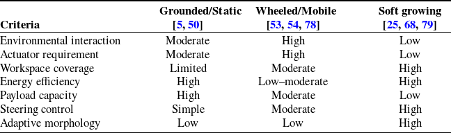


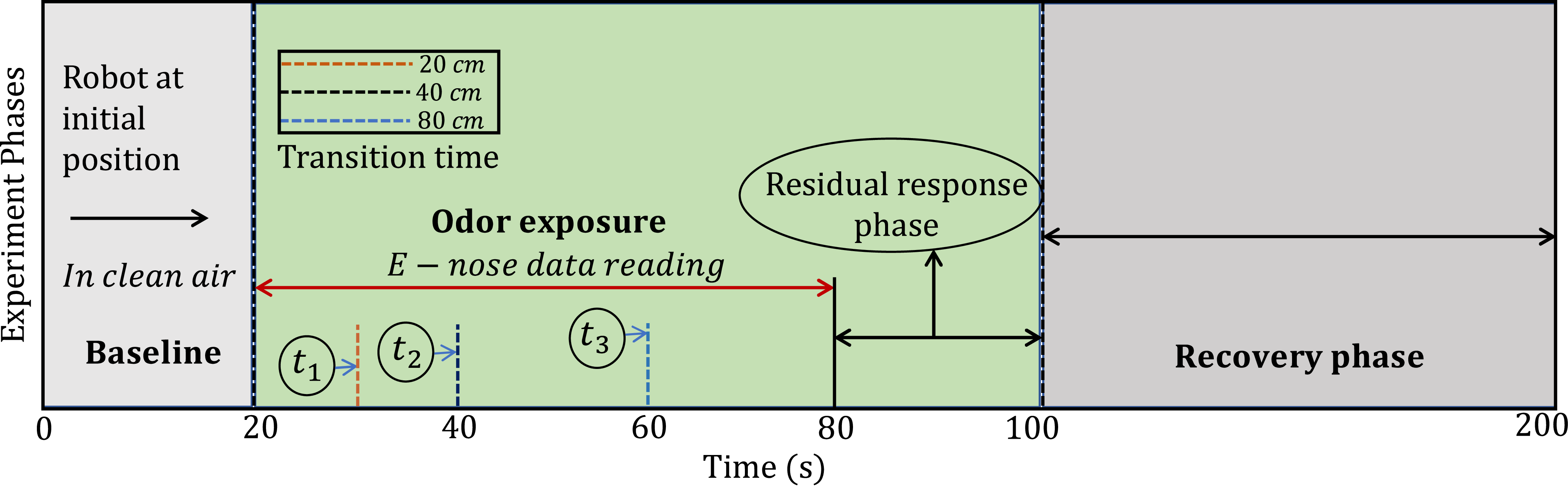


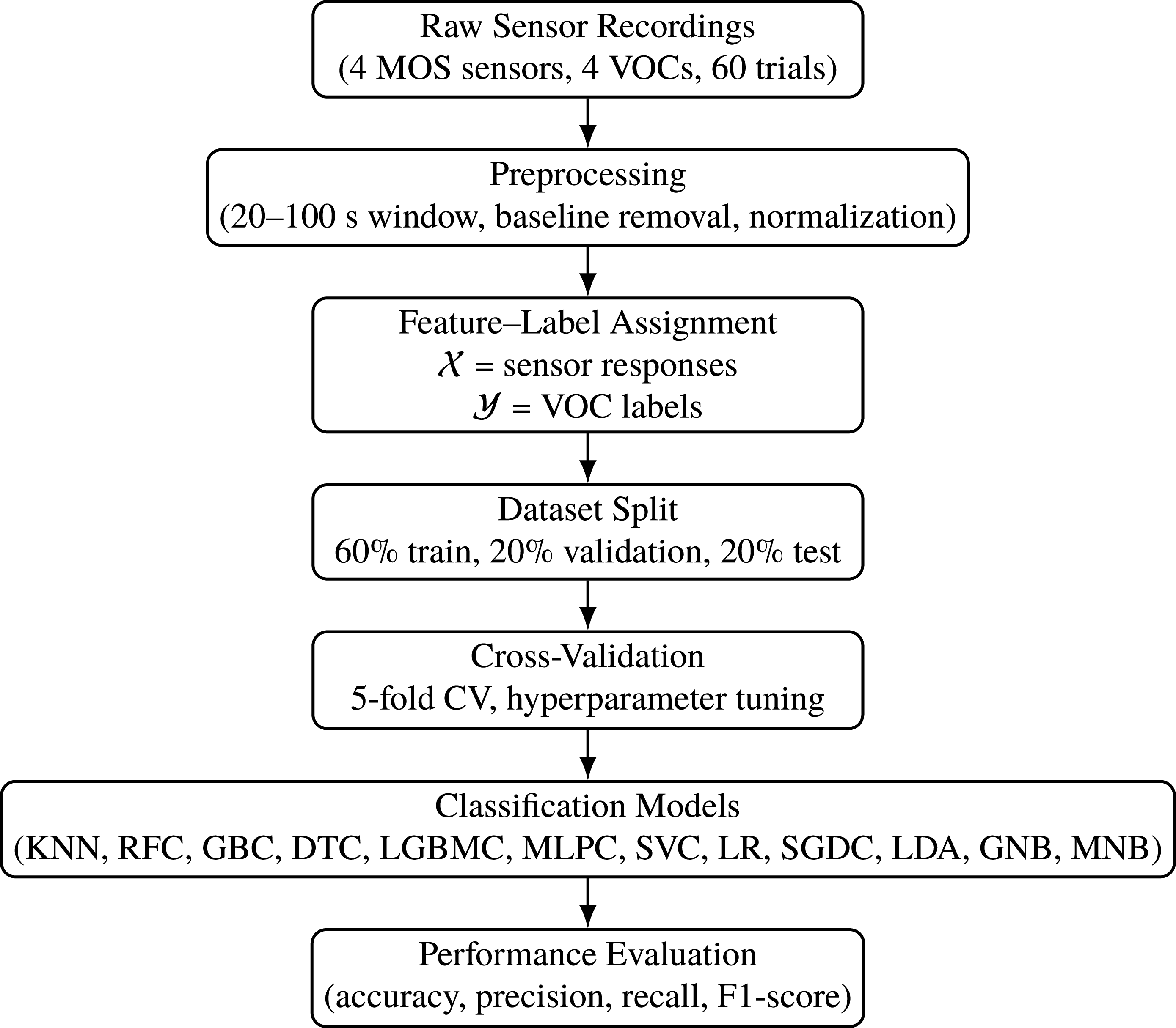
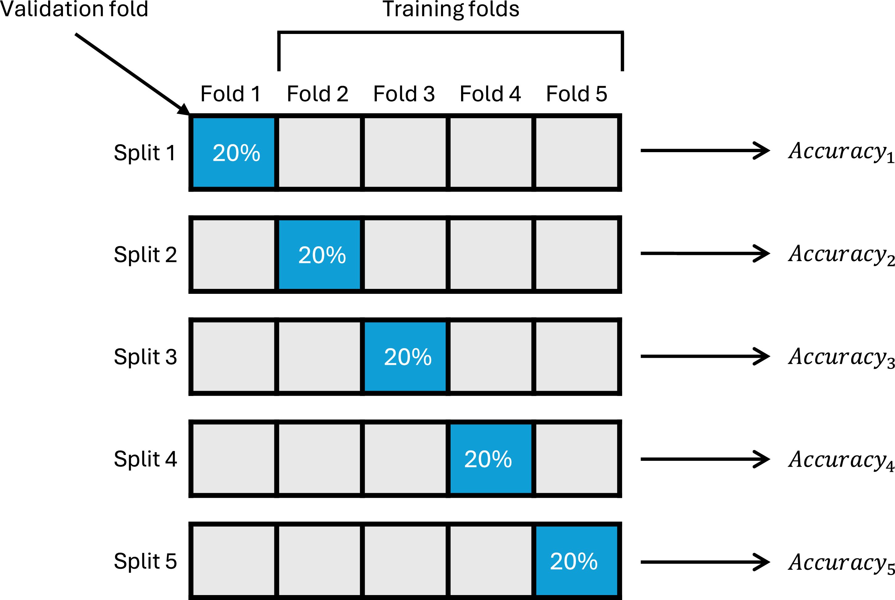


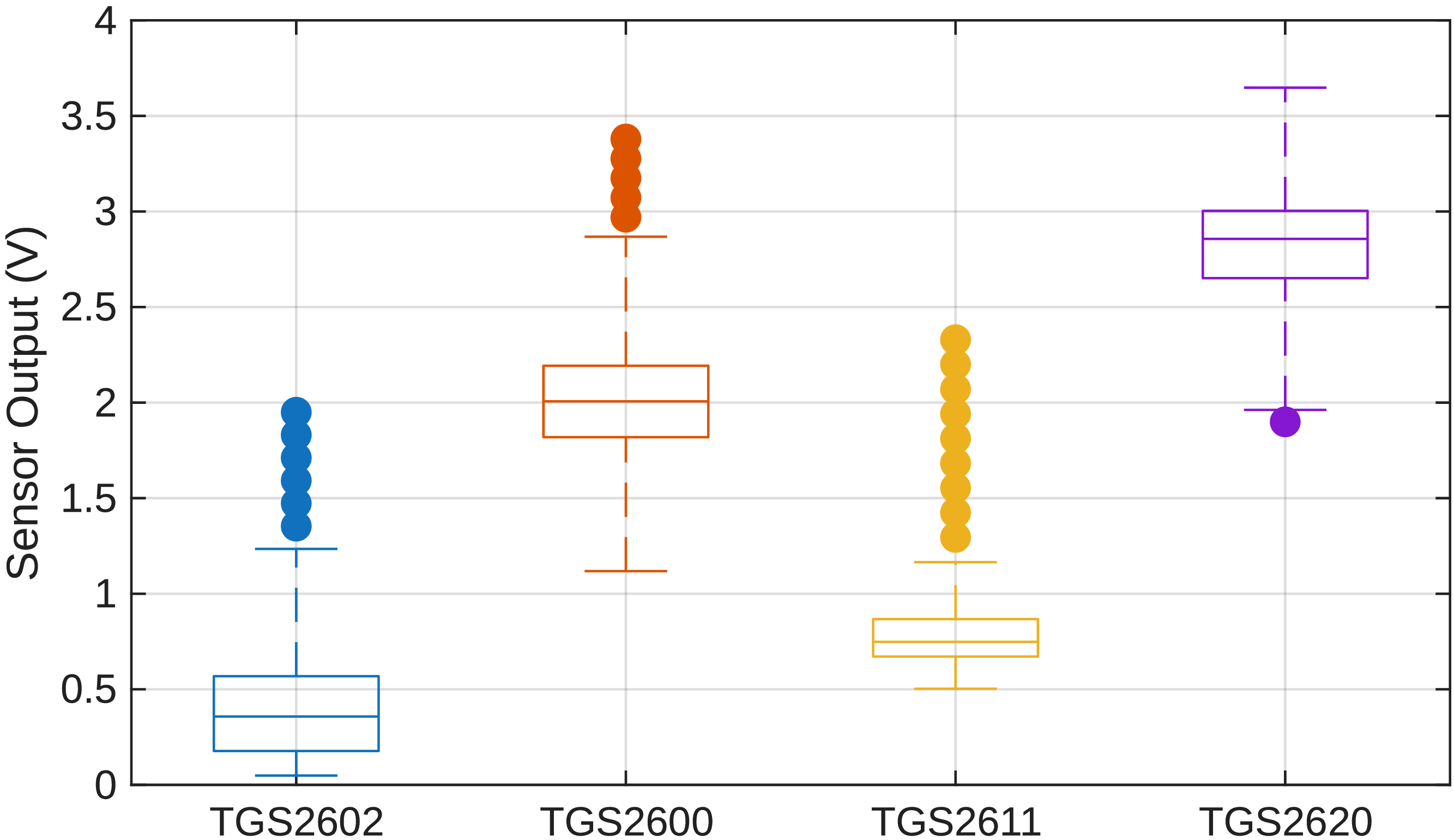
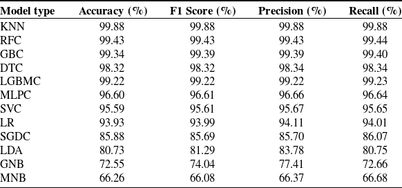


 Open access