


1. Introduction
Polymeric fluids such as plastic melts, oils, gels and paints are widespread across modern life. The presence of polymers introduces a myriad of phenomena that are not seen in simpler Newtonian fluids, due to the elasticity in the system. One key example of this is a chaotic self-sustaining state known as ‘elastic turbulence’ (ET), which is driven by elastic effects and consists of dynamics across a range of length scales (Groisman & Steinberg Reference Groisman and Steinberg2000). The addition of just a small amount of polymer into a solvent can cause it to show signs of turbulence even when inertia is negligible, distinguishing it from Newtonian turbulence.
Elastic turbulence was first identified in a curvilinear setting (Groisman & Steinberg Reference Groisman and Steinberg2000) in which hoop stresses were important in triggering the transition to turbulence (Shaqfeh Reference Shaqfeh1996). The later discovery of ET in rectilinear geometries (e.g. experimentally by Pan et al. (Reference Pan, Morozov, Wagner and Arratia2013) and Shnapp & Steinberg (Reference Shnapp and Steinberg2022) in channel flow and Bonn et al. (Reference Bonn, Ingremeau, Amarouchene and Kellay2011) in pipe flow; and numerically by Berti et al. (Reference Berti, Bistagnino, Boffetta, Celani and Musacchio2008) and Berti & Boffetta (Reference Berti and Boffetta2010) in Kolmogorov flow, Foggi Rota et al. (Reference Foggi Rota, Amor, Le Clainche and Rosti2024) and Lellep, Linkmann & Morozov (Reference Lellep, Linkmann and Morozov2024) in channel flow and Beneitez, Page & Kerswell (Reference Beneitez, Page and Kerswell2023) in plane Couette flow) where linear hoop stress instabilities are absent, demonstrated that other mechanisms can also trigger ET. Two mechanisms have recently been uncovered.
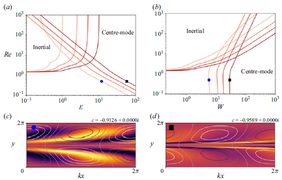
The first is the ‘centre-mode’ instability which has been identified in channel flow and pipe flow but is absent in plane Couette flow (Garg et al. Reference Garg, Chaudhary, Khalid, Shankar and Subramanian2018; Chaudhary et al. Reference Chaudhary, Garg, Subramanian and Shankar2021; Khalid et al. Reference Khalid, Chaudhary, Garg, Shankar and Subramanian2021a
,Reference Khalid, Shankar and Subramanian
b
). Despite being entirely elastic in origin (Buza et al. Reference Buza, Page and Kerswell2022b
), the instability only persists to vanishing Reynolds number in ultra-dilute channel flow (Khalid et al. Reference Khalid, Shankar and Subramanian2021b
). Significantly, the instability is subcritical in channel and pipe flow, causing instabilities at Weissenberg numbers $W$
much lower than those needed for linear instability (Page, Dubief & Kerswell Reference Page, Dubief and Kerswell2020; Wan, Sun & Zhang Reference Wan, Sun and Zhang2021; Buza et al. Reference Buza, Page and Kerswell2022b
,Reference Buza, Beneitez, Page and Kerswella; Morozov Reference Morozov2022). Solutions on the upper branch resemble ‘arrowheads’ (Page et al. Reference Page, Dubief and Kerswell2020), and these arrowhead structures can be identified within elasto-inertial turbulence in two-dimensional (2-D) channel flow when inertia is not neglected (Dubief et al. Reference Dubief, Page, Kerswell, Terrapon and Steinberg2022; Beneitez et al. Reference Beneitez, Page, Dubief and Kerswell2024a
).
$W$
much lower than those needed for linear instability (Page, Dubief & Kerswell Reference Page, Dubief and Kerswell2020; Wan, Sun & Zhang Reference Wan, Sun and Zhang2021; Buza et al. Reference Buza, Page and Kerswell2022b
,Reference Buza, Beneitez, Page and Kerswella; Morozov Reference Morozov2022). Solutions on the upper branch resemble ‘arrowheads’ (Page et al. Reference Page, Dubief and Kerswell2020), and these arrowhead structures can be identified within elasto-inertial turbulence in two-dimensional (2-D) channel flow when inertia is not neglected (Dubief et al. Reference Dubief, Page, Kerswell, Terrapon and Steinberg2022; Beneitez et al. Reference Beneitez, Page, Dubief and Kerswell2024a
).
The second new mechanism is another linear instability called the ‘polymer diffusive instability’ (PDI) which has been found very recently in plane Couette, channel and pipe flows localised at the boundaries (Beneitez et al. Reference Beneitez, Page and Kerswell2023; Couchman et al. Reference Couchman, Beneitez, Page and Kerswell2024; Lewy & Kerswell Reference Lewy and Kerswell2024). It exists in inertialess systems, and requires the presence of polymer stress diffusion, either explicitly included in the model or implicitly applied by the time-stepping numerical scheme used. It has been shown to lead to a chaotic state in three-dimensional channel flow, hinting at its relevance in the transition to wall-bounded ET (Beneitez et al. Reference Beneitez, Page and Kerswell2023, Reference Beneitez, Page, Dubief and Kerswell2024b ; Foggi Rota et al. Reference Foggi Rota, Amor, Le Clainche and Rosti2024).
In light of these developments, it seems worthwhile to revisit viscoelastic Kolmogorov flow (vKf) which was studied (Boffetta et al. Reference Boffetta, Celani, Mazzino, Puliafito and Vergassola2005) over a decade before the centre-mode instability was announced by Garg et al. (Reference Garg, Chaudhary, Khalid, Shankar and Subramanian2018) in pipe flow (at very different $Re$
) and nearly two decades before PDI was found (Beneitez et al. Reference Beneitez, Page and Kerswell2023). The original linear analysis by Boffetta et al. (Reference Boffetta, Celani, Mazzino, Puliafito and Vergassola2005) took the form of a multiscale analysis conducted at low
$Re$
) and nearly two decades before PDI was found (Beneitez et al. Reference Beneitez, Page and Kerswell2023). The original linear analysis by Boffetta et al. (Reference Boffetta, Celani, Mazzino, Puliafito and Vergassola2005) took the form of a multiscale analysis conducted at low $Re$
(
$Re$
( ${\lesssim}\,6$
) over multiple forcing wavelengths but did not plot any unstable eigenmodes. Later numerical simulation work at
${\lesssim}\,6$
) over multiple forcing wavelengths but did not plot any unstable eigenmodes. Later numerical simulation work at $Re \lesssim 1$
by Berti et al. (Reference Berti, Bistagnino, Boffetta, Celani and Musacchio2008) and Berti & Boffetta (Reference Berti and Boffetta2010), however, clearly shows arrowhead structures indicative of the centre-mode instability. A recent asymptotic analysis of the centre-mode instability (Kerswell & Page Reference Kerswell and Page2024) confirms that it exists in inertialess vKf but does not exclude the presence of other instabilities. In particular, the key ingredient for PDI may actually be maxima of the base shear, which vKf has, rather than boundaries per se, which it does not (Lewy & Kerswell Reference Lewy and Kerswell2024). Our objectives are therefore to: (i) carry out a full investigation of the linear stability problem including over multiple forcing wavelengths using Floquet analysis; (ii) clarify whether PDI exists or indeed any other elastic or elasto-inertial instability occurs beyond the known Newtonian instability; and (iii) then, armed with this information, explore the transition scenarios possible.
$Re \lesssim 1$
by Berti et al. (Reference Berti, Bistagnino, Boffetta, Celani and Musacchio2008) and Berti & Boffetta (Reference Berti and Boffetta2010), however, clearly shows arrowhead structures indicative of the centre-mode instability. A recent asymptotic analysis of the centre-mode instability (Kerswell & Page Reference Kerswell and Page2024) confirms that it exists in inertialess vKf but does not exclude the presence of other instabilities. In particular, the key ingredient for PDI may actually be maxima of the base shear, which vKf has, rather than boundaries per se, which it does not (Lewy & Kerswell Reference Lewy and Kerswell2024). Our objectives are therefore to: (i) carry out a full investigation of the linear stability problem including over multiple forcing wavelengths using Floquet analysis; (ii) clarify whether PDI exists or indeed any other elastic or elasto-inertial instability occurs beyond the known Newtonian instability; and (iii) then, armed with this information, explore the transition scenarios possible.
The structure of this paper is as follows. In § 2 the governing equations to be used are introduced, the one-dimensional base state identified and the associated linearised equations derived. The results of solving the linear instability eigenvalue problem are then discussed in § 3, where the centre-mode instability can be identified and PDI is shown to be absent. The centre mode is found to exist across a wide range of parameters in this system including an inertialess upper-convected Maxwell (UCM) fluid. We identify perturbations with a period that is twice the forcing periodicity to be the linearly most unstable using Floquet analysis. In addition, we show that the flow relaminarises at sufficiently large $W$
for a fixed geometry. We then move on to nonlinear behaviour, identifying the centre mode as subcritical in § 4, as well as plotting a range of stable exact coherent structures. Section 5 considers ET, suggesting that a bifurcation of the centre-mode instability is the cause of this chaos, and shows that the onset of turbulence is marked by the presence of bursting solutions. In addition, we see that the power spectra and energy budget of a simple periodic arrowhead solution are similar to those of ET. A final discussion is given in § 6.
$W$
for a fixed geometry. We then move on to nonlinear behaviour, identifying the centre mode as subcritical in § 4, as well as plotting a range of stable exact coherent structures. Section 5 considers ET, suggesting that a bifurcation of the centre-mode instability is the cause of this chaos, and shows that the onset of turbulence is marked by the presence of bursting solutions. In addition, we see that the power spectra and energy budget of a simple periodic arrowhead solution are similar to those of ET. A final discussion is given in § 6.
2. Formulation
We consider 2-D Kolmogorov flow of an Oldroyd-B fluid with forcing in the $\hat{\mathbf{x}}$
direction that varies periodically with
$\hat{\mathbf{x}}$
direction that varies periodically with $\hat{\mathbf{y}}$
in the perpendicular direction. The non-dimensionalised equations relating the velocity
$\hat{\mathbf{y}}$
in the perpendicular direction. The non-dimensionalised equations relating the velocity $\mathbf {u}$
, the polymeric stress tensor
$\mathbf {u}$
, the polymeric stress tensor $\mathbf {T}$
, the conformation tensor
$\mathbf {T}$
, the conformation tensor $\mathbf {C}$
and the pressure
$\mathbf {C}$
and the pressure $p$
are
$p$
are
 \begin{align} Re \left(\frac {\partial \mathbf {u}}{\partial t} + \mathbf {u} \cdot \nabla \mathbf {u}\right) = - \nabla p + (1-\beta ) \nabla \cdot \mathbf {T} + \beta \nabla ^2 \mathbf {u} + \left (\frac {1+\varepsilon \beta W}{1+\varepsilon W}\right ) \cos y \, \hat{\mathbf{x}}, \end{align}
 \begin{align} \frac {\partial {\mathbf {C}}}{\partial t} + \mathbf {u} \cdot \nabla \mathbf {C} - \nabla \mathbf {u}^T \cdot \mathbf {C} - \mathbf {C} \cdot \nabla \mathbf {u} + \mathbf {T} = \varepsilon \nabla ^2 \mathbf {C}, \end{align}
 \begin{align} \nabla \cdot \mathbf {u} = 0 \end{align}
and
 \begin{align} \mathbf {T} = \frac {1}{W}(\mathbf {C}-\mathbf {I}). \end{align}
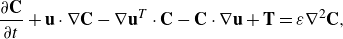
We consider a domain of size $[0, L_x] \times [0, 2\pi n]$
, where
$[0, L_x] \times [0, 2\pi n]$
, where $L_x$
is the horizontal extent and the integer
$L_x$
is the horizontal extent and the integer $n$
is the number of forcing wavelengths applied to the system (see figure 1). Periodic boundary conditions are imposed in both directions, so, in particular, flows with a wavelength
$n$
is the number of forcing wavelengths applied to the system (see figure 1). Periodic boundary conditions are imposed in both directions, so, in particular, flows with a wavelength $n$
times longer than the forcing are permitted. All variables are scaled using the laminar peak velocity
$n$
times longer than the forcing are permitted. All variables are scaled using the laminar peak velocity $U_0$
, the total viscosity
$U_0$
, the total viscosity $\mu = \mu _s + \mu _p$
, which is the sum of the solvent and polymer viscosities, respectively, and the length scale
$\mu = \mu _s + \mu _p$
, which is the sum of the solvent and polymer viscosities, respectively, and the length scale $L_0/2\pi$
, where
$L_0/2\pi$
, where $L_0$
is the forcing wavelength. The coefficient of the forcing term in (2.1) is to ensure that the resulting base velocity has unit amplitude.
$L_0$
is the forcing wavelength. The coefficient of the forcing term in (2.1) is to ensure that the resulting base velocity has unit amplitude.
The Kolmogorov flow set-up with forcing wavelength $2\pi$
. Perturbations have wavelength
$2\pi$
. Perturbations have wavelength $2\pi n$
in the
$2\pi n$
in the $\hat{\mathbf{y}}$
direction (where
$\hat{\mathbf{y}}$
direction (where $n$
is an integer) and
$n$
is an integer) and $L_x$
in the
$L_x$
in the $\hat{\mathbf{x}}$
direction.
$\hat{\mathbf{x}}$
direction.
These equations use dimensionless parameters:
 \begin{align} Re := \frac {\rho U_0 L_0}{2 \pi \mu }, \qquad W := \frac {2 \pi U_0 \lambda }{L_0}, \end{align}
 \begin{align} \beta := \frac {\mu _s}{\mu }, \qquad \varepsilon := \frac {2 \pi \delta }{U_0 L_0}, \\[6pt] \nonumber \end{align}
where $\rho$
is the density,
$\rho$
is the density, $\lambda$
is the relaxation time and
$\lambda$
is the relaxation time and $\delta$
is the polymer stress diffusion coefficient. It will be useful to define the elasticity number:
$\delta$
is the polymer stress diffusion coefficient. It will be useful to define the elasticity number:
 \begin{align} E := \frac {W}{Re} \end{align}
which is the measure of elasticity used to introduce the centre-mode instability (Garg et al. Reference Garg, Chaudhary, Khalid, Shankar and Subramanian2018; Khalid et al. Reference Khalid, Chaudhary, Garg, Shankar and Subramanian2021a
; Chaudhary et al. Reference Chaudhary, Garg, Subramanian and Shankar2021). The Oldroyd-B model reduces to the UCM when the concentration $\beta =0$
.
$\beta =0$
.
2.1. Symmetries
The above system has three types of symmetries associated with it, like in the Newtonian case (Chandler & Kerswell Reference Chandler and Kerswell2013). The shift-reflect symmetry maps
 \begin{align} \mathcal {S} [u, v, T_{xx}, T_{xy}, T_{yy}, p](x, y) \rightarrow [{-}u, v, T_{xx}, -T_{xy}, T_{yy}, p]({-}x, y+\pi ), \end{align}
where $\mathbf {u} = u \hat{\mathbf{x}} + v \hat{\mathbf{y}}$
and
$\mathbf {u} = u \hat{\mathbf{x}} + v \hat{\mathbf{y}}$
and $\mathbf {T} = T_{xx} \hat{\mathbf{x}}\hat{\mathbf{x}} + T_{xy} (\hat{\mathbf{x}}\hat{\mathbf{y}} + \hat{\mathbf{y}}\hat{\mathbf{x}}) + T_{yy}\hat{\mathbf{y}}\hat{\mathbf{y}}$
. A reflection symmetry maps
$\mathbf {T} = T_{xx} \hat{\mathbf{x}}\hat{\mathbf{x}} + T_{xy} (\hat{\mathbf{x}}\hat{\mathbf{y}} + \hat{\mathbf{y}}\hat{\mathbf{x}}) + T_{yy}\hat{\mathbf{y}}\hat{\mathbf{y}}$
. A reflection symmetry maps
 \begin{align} \mathcal {R}[u, v, T_{xx}, T_{xy}, T_{yy}, p](x, y) \rightarrow [u, -v, T_{xx}, -T_{xy}, T_{yy}, p](x, 2\pi -y). \end{align}
In addition to these two discrete symmetries, there is the continuous translational symmetry
 \begin{align} \mathcal {T}_s[u, v, T_{xx}, T_{xy}, T_{yy}, p](x, y) \rightarrow [u, v, T_{xx}, T_{xy}, T_{yy}, p](x+s, y) \end{align}
for $s \in [0, L_x)$
. Every solution is therefore associated with a set of solutions generated via these symmetries, and in particular the shift-reflect symmetry means that any solution moving in the positive
$s \in [0, L_x)$
. Every solution is therefore associated with a set of solutions generated via these symmetries, and in particular the shift-reflect symmetry means that any solution moving in the positive $\hat{\mathbf{x}}$
direction has an associated solution moving in the negative
$\hat{\mathbf{x}}$
direction has an associated solution moving in the negative $\hat{\mathbf{x}}$
direction.
$\hat{\mathbf{x}}$
direction.
2.2. Base flow
There is a one-dimensional base flow which depends only on $y$
which is
$y$
which is
 \begin{align} \mathbf {U} = \cos y \, \hat{\mathbf{x}}, \quad P=0, \end{align}
 \begin{align} T_{xx} = \frac {W}{1+\varepsilon W} \left (1 - \frac {\cos 2y}{1+4\varepsilon W}\right ), \quad T_{xy} = \frac {-1}{1+\varepsilon W} \sin y \quad \textrm{and} \quad T_{yy} = 0. \\[6pt] \nonumber \end{align}
2.3. Linearising
To examine the linear stability of the base state, small perturbations proportional to $\textrm{e}^{ik(x-ct)}$
of all dependent variables are considered where
$\textrm{e}^{ik(x-ct)}$
of all dependent variables are considered where $k\in \mathbb {R}$
is the wavenumber, and
$k\in \mathbb {R}$
is the wavenumber, and $c \in \mathbb {C}$
is an eigenvalue to be found. This results in variables of the form
$c \in \mathbb {C}$
is an eigenvalue to be found. This results in variables of the form
 \begin{align} \mathbf {u} &= \mathbf {U}(y)+ \begin{bmatrix} u^{\prime}(y) \\ v^{\prime}(y) \end{bmatrix} \textrm{e}^{ik(x-ct)}, \quad p = p^{\prime}(y)\textrm{e}^{ik(x-ct)} \nonumber \\ \mathbf {T} &= \mathbf {T}(y) + \left[\begin{array}{l@{\quad}l} \tau _{xx}^{\prime}(y) & \tau _{xy}^{\prime}(y) \\[3pt] \tau _{xy}^{\prime}(y) & \tau _{yy}^{\prime}(y) \end{array} \right]\textrm{e}^{ik(x-ct)}, \end{align}
where a prime denotes a perturbative quantity that, due to the boundary conditions, must be $2\pi n$
periodic in
$2\pi n$
periodic in $y$
. The imaginary part of the eigenvalue,
$y$
. The imaginary part of the eigenvalue, $c_i$
, determines the linear stability of the system, with
$c_i$
, determines the linear stability of the system, with $\sigma := kc_i$
the growth rate. To reduce slightly the linearised equations which determine the evolution of the perturbations, we take the curl of (2.1) to eliminate the pressure, and use (2.4) to write all
$\sigma := kc_i$
the growth rate. To reduce slightly the linearised equations which determine the evolution of the perturbations, we take the curl of (2.1) to eliminate the pressure, and use (2.4) to write all $\mathbf {C}$
in terms of
$\mathbf {C}$
in terms of $\mathbf {T}$
. Equations (2.1)–(2.4) then become
$\mathbf {T}$
. Equations (2.1)–(2.4) then become
 \begin{align} ikRe \big[ (U-c)\big(D^2-k^2 \big) - D^2U\big]v^{\prime} = &-(1-\beta )\big [ -k^2 D\big(\tau _{xx}^{\prime} - {\tau _{yy}^{\prime}}\big) + ik \big(D^2 + {k^2}\big) \tau _{xy}^{\prime} \big ] \nonumber \\ &+ \beta \big( D^2 - {k^2}\big)^2 v^{\prime}, \end{align}
 \begin{align} \big [ik(U-c) + \frac {1}{W} - \varepsilon \big(D^2 - k^2 \big) \big ]\tau _{xx}^{\prime} & = -v^{\prime}DT_{xx} + 2ikT_{xx} u^{\prime} + 2T_{xy} Du^{\prime} + 2\tau _{xy}^{\prime}DU \nonumber\\ & \quad+ {\frac {2ik}{W}u^{\prime}} , \end{align}
 \begin{align} \big [ik(U-c) + \frac {1}{W}- \varepsilon \big(D^2 - k^2 \big)\big ]\tau _{xy}^{\prime} & = -v^{\prime}DT_{xy} + ikT_{xx} v^{\prime} + \tau _{yy}^{\prime}DU \nonumber \\ & + \frac {1}{W} \big(Du^{\prime} + {ikv^{\prime}}\big) , \end{align}
 \begin{align} \big [ik(U-c) + \frac {1}{W}- \varepsilon \big(D^2 - k^2 \big)\big ]\tau _{yy}^{\prime} = 2ikT_{xy} v^{\prime} + \frac {2}{W}Dv^{\prime} , \end{align}
 \begin{align} iku^{\prime} + Dv^{\prime} = 0 ,\end{align}
where $D:= \textrm{d}/\textrm{d}y$
. The costly procedure of solving this eigenvalue problem over the whole domain
$D:= \textrm{d}/\textrm{d}y$
. The costly procedure of solving this eigenvalue problem over the whole domain $y\in [0,2\pi n]$
can be avoided by applying Floquet analysis just across one forcing wavelength
$y\in [0,2\pi n]$
can be avoided by applying Floquet analysis just across one forcing wavelength $y\in [0,2\pi ]$
and including a modulation parameter
$y\in [0,2\pi ]$
and including a modulation parameter $\mu$
to compensate. A mode with Floquet exponent
$\mu$
to compensate. A mode with Floquet exponent $\mu$
has perturbations of the form
$\mu$
has perturbations of the form $\phi ^{\prime} = \hat \phi (y) \textrm{e}^{i\mu y}$
, where
$\phi ^{\prime} = \hat \phi (y) \textrm{e}^{i\mu y}$
, where $\phi ^{\prime}$
is the perturbation of any flow variable and
$\phi ^{\prime}$
is the perturbation of any flow variable and $\hat \phi$
is
$\hat \phi$
is $2\pi$
periodic. The resultant perturbation has periodicity
$2\pi$
periodic. The resultant perturbation has periodicity $2\pi / \mu$
when
$2\pi / \mu$
when $1/\mu \in \mathbb {N}$
, as all base flow quantities have the same periodicity as the forcing. Values of
$1/\mu \in \mathbb {N}$
, as all base flow quantities have the same periodicity as the forcing. Values of $1/\mu$
which factor into
$1/\mu$
which factor into $n$
then satisfy the periodic boundary conditions over the large domain of
$n$
then satisfy the periodic boundary conditions over the large domain of $y\in [0,2\pi n]$
.
$y\in [0,2\pi n]$
.
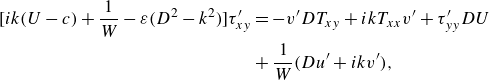
The eigenvalue spectrum when $E=81$
,
$E=81$
, $Re=2$
,
$Re=2$
, $\beta =0.95$
,
$\beta =0.95$
, $\varepsilon =0$
,
$\varepsilon =0$
, $\mu =0$
and
$\mu =0$
and $k=0.2$
, with resolution
$k=0.2$
, with resolution $N_y=300$
(blue circles) and
$N_y=300$
(blue circles) and $N_y=400$
(red dots), where
$N_y=400$
(red dots), where $N_y$
is the number of Chebyshev modes considered in the eigenvalue problem. The centre mode has unstable eigenvalues at
$N_y$
is the number of Chebyshev modes considered in the eigenvalue problem. The centre mode has unstable eigenvalues at $\text{c}=\pm 1.01016736+0.05925964i$
, while a stable continuous spectrum is seen with
$\text{c}=\pm 1.01016736+0.05925964i$
, while a stable continuous spectrum is seen with $c_i\lt 0$
. Insets show the polymer stress trace (colours) and streamfunction (contours) of an eigenmode
$c_i\lt 0$
. Insets show the polymer stress trace (colours) and streamfunction (contours) of an eigenmode $\phi$
, alongside symmetries of
$\phi$
, alongside symmetries of $\phi$
. While reflections
$\phi$
. While reflections $\mathcal {R}$
and translations
$\mathcal {R}$
and translations $\mathcal {T}_s$
leave the eigenvalue
$\mathcal {T}_s$
leave the eigenvalue $c=c_r+ic_i$
unchanged, shift-reflections
$c=c_r+ic_i$
unchanged, shift-reflections $\mathcal {S}$
produce modes with eigenvalue
$\mathcal {S}$
produce modes with eigenvalue $-c_r+ic_i$
that travel in the opposite direction.
$-c_r+ic_i$
that travel in the opposite direction.
3. Linear instability
In this section, the linear instability seen in vKf by Boffetta et al. (Reference Boffetta, Celani, Mazzino, Puliafito and Vergassola2005) is identified as the centre-mode instability (Garg et al. Reference Garg, Chaudhary, Khalid, Shankar and Subramanian2018; Chaudhary et al. Reference Chaudhary, Garg, Subramanian and Shankar2021; Khalid et al. Reference Khalid, Chaudhary, Garg, Shankar and Subramanian2021a
). We begin by considering vKf when the flow has the same spatial periodicity as the forcing (i.e. $n=1$
), and see that: (i) the instability scales with
$n=1$
), and see that: (i) the instability scales with $E$
like the centre mode in a channel when
$E$
like the centre mode in a channel when $E\ll 1$
and (ii) the eigenfunction resembles the centre mode. We then consider
$E\ll 1$
and (ii) the eigenfunction resembles the centre mode. We then consider $E\gg 1$
, as well as how increasing
$E\gg 1$
, as well as how increasing $n$
, the number of forcing wavelengths, affects the instability. The centre-mode instability is not confined to dilute vKf, but is found across all
$n$
, the number of forcing wavelengths, affects the instability. The centre-mode instability is not confined to dilute vKf, but is found across all $\beta \in [0,1)$
, even existing for a UCM fluid with
$\beta \in [0,1)$
, even existing for a UCM fluid with $\beta =0$
. Curiously, the flow is also found to restabilise as
$\beta =0$
. Curiously, the flow is also found to restabilise as $W\rightarrow \infty$
within a geometry of fixed streamwise extent. All numerics were computed using spectral solvers from the open-source software Dedalus (Burns et al. Reference Burns, Vasil, Oishi, Lecoanet and Brown2020). Our code was verified by (i) reproducing eigenvalues from Kerswell & Page (Reference Kerswell and Page2024) where the Floquet exponent was
$W\rightarrow \infty$
within a geometry of fixed streamwise extent. All numerics were computed using spectral solvers from the open-source software Dedalus (Burns et al. Reference Burns, Vasil, Oishi, Lecoanet and Brown2020). Our code was verified by (i) reproducing eigenvalues from Kerswell & Page (Reference Kerswell and Page2024) where the Floquet exponent was $\mu =0$
and (ii) ensuring growth rates obtained using our eigenvalue solver agree with those obtained using our timestepper code (checked when Floquet exponent
$\mu =0$
and (ii) ensuring growth rates obtained using our eigenvalue solver agree with those obtained using our timestepper code (checked when Floquet exponent $\mu =0, 1/2$
).
$\mu =0, 1/2$
).
3.1.
Harmonic disturbances ( $n=1$
)
$n=1$
)

Kerswell & Page (Reference Kerswell and Page2024) show that there is an unstable eigenfunction when $n=1$
in ultra-dilute vKf that resembles the centre-mode eigenfunction in a channel. Here we go a step further and show that the
$n=1$
in ultra-dilute vKf that resembles the centre-mode eigenfunction in a channel. Here we go a step further and show that the $(Re,k)$
neutral curves show the distinctive centre-mode loops seen in channel flow (as shown in figure 10 of Khalid et al. (Reference Khalid, Chaudhary, Garg, Shankar and Subramanian2021a)), and they follow the same scaling relation for
$(Re,k)$
neutral curves show the distinctive centre-mode loops seen in channel flow (as shown in figure 10 of Khalid et al. (Reference Khalid, Chaudhary, Garg, Shankar and Subramanian2021a)), and they follow the same scaling relation for $E \ll 1$
. However, we also show that the behaviour for large
$E \ll 1$
. However, we also show that the behaviour for large $E$
is substantially different in this unbounded flow from that of the centre mode in channel flow, as the instability is not suppressed as
$E$
is substantially different in this unbounded flow from that of the centre mode in channel flow, as the instability is not suppressed as $E\rightarrow \infty$
. Instead, the instability exists in inertialess vKf.
$E\rightarrow \infty$
. Instead, the instability exists in inertialess vKf.
To consider the system with $n=1$
we take the linearised system with Floquet exponent
$n=1$
we take the linearised system with Floquet exponent $\mu = 0$
. We plot an example eigenvalue spectrum in figure 2, showing how an eigenmode and its eigenvalue
$\mu = 0$
. We plot an example eigenvalue spectrum in figure 2, showing how an eigenmode and its eigenvalue $c=c_r+ic_i$
are affected by the symmetries discussed in § 2.1. The shift-reflect symmetry
$c=c_r+ic_i$
are affected by the symmetries discussed in § 2.1. The shift-reflect symmetry $\mathcal {S}$
generates a new eigenmode with eigenvalue
$\mathcal {S}$
generates a new eigenmode with eigenvalue $c=-c_r+ic_i$
that travels in the opposite direction. The symmetries of the centre mode in the
$c=-c_r+ic_i$
that travels in the opposite direction. The symmetries of the centre mode in the $n=1$
case make the eigenmode invariant under reflection
$n=1$
case make the eigenmode invariant under reflection $\mathcal {R}$
. Lastly, translational symmetries
$\mathcal {R}$
. Lastly, translational symmetries $\mathcal {T}_s$
correspond to a phase shift of the mode. The stability of all such symmetries is the same, as the growth rate is unchanged under all operators.
$\mathcal {T}_s$
correspond to a phase shift of the mode. The stability of all such symmetries is the same, as the growth rate is unchanged under all operators.
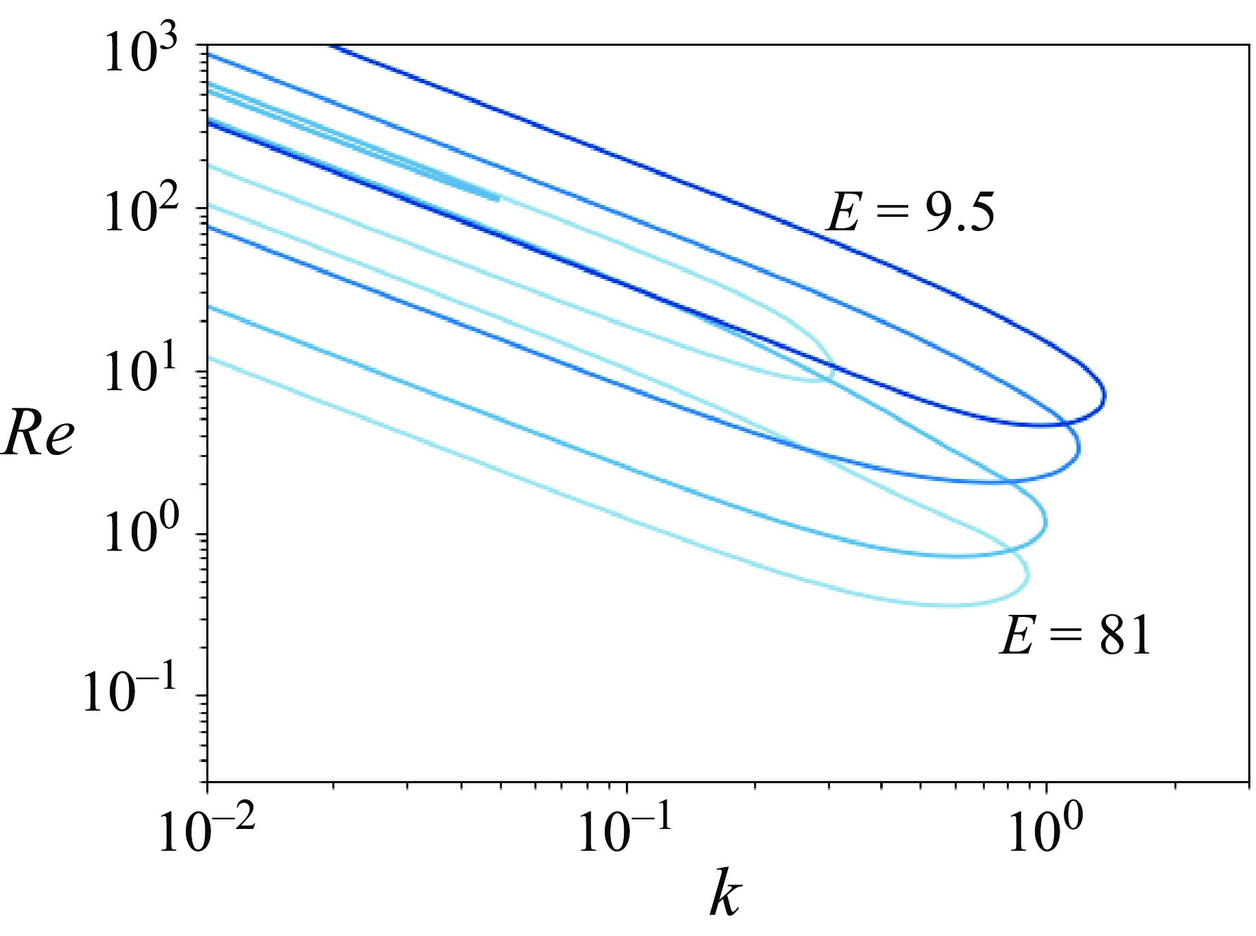
 $(a{-}d)$
The centre-mode neutral curves in the
$(a{-}d)$
The centre-mode neutral curves in the $(Re, k)$
plane for
$(Re, k)$
plane for $\beta =0.95$
,
$\beta =0.95$
, $\varepsilon =0$
,
$\varepsilon =0$
, $\mu =0$
and
$\mu =0$
and $(a, b)$ $E = 0.3, 0.6, 1.0, 1.8, 3.1, 5.5, 9.5$
(light to dark) and
$E = 0.3, 0.6, 1.0, 1.8, 3.1, 5.5, 9.5$
(light to dark) and $(c, d)$ $E=81, 107, 142, 187, 272, 359, 475$
(light to dark). Note that
$E=81, 107, 142, 187, 272, 359, 475$
(light to dark). Note that $(b,d)$
are scaled versions of
$(b,d)$
are scaled versions of $(a,c)$
, respectively, demonstrating that for small
$(a,c)$
, respectively, demonstrating that for small $E$
,
$E$
, $Re_{crit} \sim E^{-3/2}$
, while for large
$Re_{crit} \sim E^{-3/2}$
, while for large $E$
,
$E$
, $Re_{crit} \sim E^{-1}$
. We plot eigenfunctions with
$Re_{crit} \sim E^{-1}$
. We plot eigenfunctions with $k=0.2$
and (e)
$k=0.2$
and (e) $E=3.1, Re=300$
, (f)
$E=3.1, Re=300$
, (f) $E=81, Re=2$
and (g)
$E=81, Re=2$
and (g) $E=81, Re=20$
. These correspond to the instability in the low-
$E=81, Re=20$
. These correspond to the instability in the low- $E$
regime, the main loop in the high-
$E$
regime, the main loop in the high- $E$
regime and the secondary loop in the high-
$E$
regime and the secondary loop in the high- $E$
regime, respectively. Colours show the polymer stress trace field, while contours show the streamfunction. This figure demonstrates that the elastic instability seen at high
$E$
regime, respectively. Colours show the polymer stress trace field, while contours show the streamfunction. This figure demonstrates that the elastic instability seen at high $\beta$
and low
$\beta$
and low $E$
is the centre mode, and that a different scaling regime exists at high
$E$
is the centre mode, and that a different scaling regime exists at high $E$
.
$E$
.
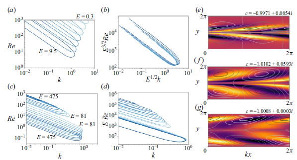
Figures 3(a) and 3(b) show unscaled and scaled $(Re,k)$
neutral curves for small values of
$(Re,k)$
neutral curves for small values of $E$
. The neutral curves take the form of loops at small
$E$
. The neutral curves take the form of loops at small $E$
, as is the case in channel flow. For these loops,
$E$
, as is the case in channel flow. For these loops, $Re_{crit} \sim E^{-3/2}$
and
$Re_{crit} \sim E^{-3/2}$
and $k_{crit} \sim E^{-1/2}$
, where
$k_{crit} \sim E^{-1/2}$
, where $Re_{crit}$
denotes the smallest Reynolds number on the neutral curve and
$Re_{crit}$
denotes the smallest Reynolds number on the neutral curve and $k_{crit}$
denotes the wavenumber at that point. These match the scalings for the centre mode in channel flow (Khalid et al. Reference Khalid, Chaudhary, Garg, Shankar and Subramanian2021a
). An eigenfunction in this regime is plotted in figure 3(e), resembling that of the channel flow centre mode as seen in figure 5 of Khalid et al. (Reference Khalid, Chaudhary, Garg, Shankar and Subramanian2021a
). The scaling relation and the eigenfunction both suggest that this instability is the centre mode.
$k_{crit}$
denotes the wavenumber at that point. These match the scalings for the centre mode in channel flow (Khalid et al. Reference Khalid, Chaudhary, Garg, Shankar and Subramanian2021a
). An eigenfunction in this regime is plotted in figure 3(e), resembling that of the channel flow centre mode as seen in figure 5 of Khalid et al. (Reference Khalid, Chaudhary, Garg, Shankar and Subramanian2021a
). The scaling relation and the eigenfunction both suggest that this instability is the centre mode.
Figures 3(c) and 3(d) show the neutral curves for large $E$
. The behaviour here is substantially different from that of channel and pipe flow, where at sufficiently large
$E$
. The behaviour here is substantially different from that of channel and pipe flow, where at sufficiently large $E$
the centre mode is suppressed (Khalid et al. Reference Khalid, Chaudhary, Garg, Shankar and Subramanian2021a
; Chaudhary et al. Reference Chaudhary, Garg, Subramanian and Shankar2021). Here in vKf, the instability exists at all
$E$
the centre mode is suppressed (Khalid et al. Reference Khalid, Chaudhary, Garg, Shankar and Subramanian2021a
; Chaudhary et al. Reference Chaudhary, Garg, Subramanian and Shankar2021). Here in vKf, the instability exists at all $E$
(only up to
$E$
(only up to $E=475$
is shown), and we see that the loops have
$E=475$
is shown), and we see that the loops have $Re_{crit} \sim E^{-1}$
and
$Re_{crit} \sim E^{-1}$
and $k_{crit} \sim E^0$
as
$k_{crit} \sim E^0$
as $E \rightarrow \infty$
. Equivalently one can consider the scalings in terms of
$E \rightarrow \infty$
. Equivalently one can consider the scalings in terms of $Re$
and
$Re$
and $W$
to obtain that as
$W$
to obtain that as $Re \rightarrow 0$
for fixed
$Re \rightarrow 0$
for fixed $W$
,
$W$
, $W_{crit} \sim Re^0$
and
$W_{crit} \sim Re^0$
and $k_{crit} \sim Re^0$
, meaning these critical parameters are independent of
$k_{crit} \sim Re^0$
, meaning these critical parameters are independent of $Re$
. While
$Re$
. While $Re_{crit}$
and
$Re_{crit}$
and $k_{crit}$
are on a loop with these scalings, a secondary loop also exists at larger
$k_{crit}$
are on a loop with these scalings, a secondary loop also exists at larger $Re$
. These secondary loops collapse as
$Re$
. These secondary loops collapse as $E$
increases. It is worth pointing out that in this regime, the largest streamwise wavenumber at which instability is seen is
$E$
increases. It is worth pointing out that in this regime, the largest streamwise wavenumber at which instability is seen is $k \approx 0.9$
, and hence no linear instability is seen when simulating a box with
$k \approx 0.9$
, and hence no linear instability is seen when simulating a box with $L_x=2\pi$
and
$L_x=2\pi$
and $n=1$
, as is true in the Newtonian case (Marchioro Reference Marchioro1986). The eigenfunctions for large
$n=1$
, as is true in the Newtonian case (Marchioro Reference Marchioro1986). The eigenfunctions for large $E$
are seen in figures 3(f) and 3(g), showing the main loop and the secondary loop, respectively. The eigenfunctions on the secondary loop visually resemble that of the main loop, though activity is more spread out across the flow and less clearly localised to
$E$
are seen in figures 3(f) and 3(g), showing the main loop and the secondary loop, respectively. The eigenfunctions on the secondary loop visually resemble that of the main loop, though activity is more spread out across the flow and less clearly localised to $y=\pi$
. Both visibly resemble the centre-mode eigenfunction in the low-
$y=\pi$
. Both visibly resemble the centre-mode eigenfunction in the low- $E$
regime in figure 3(e). To further demonstrate that the high-
$E$
regime in figure 3(e). To further demonstrate that the high- $E$
instabilities are the centre mode, figure 4 shows that the neutral curve loops from the high-
$E$
instabilities are the centre mode, figure 4 shows that the neutral curve loops from the high- $E$
regime continuously track into the loops from the low-
$E$
regime continuously track into the loops from the low- $E$
regime. This means that the centre mode is responsible for the instability across all values of
$E$
regime. This means that the centre mode is responsible for the instability across all values of $E$
.
$E$
.
The centre-mode neutral curves in the $(Re, k)$
plane for
$(Re, k)$
plane for $\beta =0.95$
,
$\beta =0.95$
, $\varepsilon =0$
,
$\varepsilon =0$
, $\mu =0$
and
$\mu =0$
and $E = 9.5, 17, 41, 81$
(dark to light). Secondary loops exist for the
$E = 9.5, 17, 41, 81$
(dark to light). Secondary loops exist for the $E=41, 81$
curves. This shows that the neutral curve loops from the low-
$E=41, 81$
curves. This shows that the neutral curve loops from the low- $E$
regime (
$E$
regime ( $E\lt 9.5$
) can be continuously tracked into the main loops in the high-
$E\lt 9.5$
) can be continuously tracked into the main loops in the high- $E$
regime (
$E$
regime ( $E\gt 81$
).
$E\gt 81$
).
The neutral curves in the $(Re, E)$
and
$(Re, E)$
and $(Re, W)$
planes are shown in figure 5. These demonstrate that the centre-mode instability is linearly unstable at vanishing
$(Re, W)$
planes are shown in figure 5. These demonstrate that the centre-mode instability is linearly unstable at vanishing $Re$
in vKf over a range of concentrations
$Re$
in vKf over a range of concentrations $\beta$
. This contrasts with the cases of inertialess pipe flow, which is linearly stable (Chaudhary et al. Reference Chaudhary, Garg, Subramanian and Shankar2021), and inertialess channel flow, which is only linearly unstable for ultra-dilute fluids with
$\beta$
. This contrasts with the cases of inertialess pipe flow, which is linearly stable (Chaudhary et al. Reference Chaudhary, Garg, Subramanian and Shankar2021), and inertialess channel flow, which is only linearly unstable for ultra-dilute fluids with $\beta \gt 0.9905$
(Khalid et al. Reference Khalid, Chaudhary, Garg, Shankar and Subramanian2021a
,Reference Khalid, Shankar and Subramanian
b
).
$\beta \gt 0.9905$
(Khalid et al. Reference Khalid, Chaudhary, Garg, Shankar and Subramanian2021a
,Reference Khalid, Shankar and Subramanian
b
).
The neutral curves also show a second instability, which exists at vanishing $W$
and is inertial in nature. This instability is seen in Newtonian Kolmogorov flow, with a purely imaginary eigenvalue
$W$
and is inertial in nature. This instability is seen in Newtonian Kolmogorov flow, with a purely imaginary eigenvalue $c$
(Meshalkin & Sinai Reference Meshalkin and Sinai1961) and we identify an instability as inertial here if it similarly has zero frequency. This instability is suppressed by elasticity, with there being a maximum
$c$
(Meshalkin & Sinai Reference Meshalkin and Sinai1961) and we identify an instability as inertial here if it similarly has zero frequency. This instability is suppressed by elasticity, with there being a maximum $E$
at which it exists.
$E$
at which it exists.
The neutral curves across $k\in \mathbb {R}$
in the (a)
$k\in \mathbb {R}$
in the (a) $(Re, E)$
and (b)
$(Re, E)$
and (b) $(Re, W)$
planes when
$(Re, W)$
planes when $\varepsilon =0$
,
$\varepsilon =0$
, $\mu =0$
and
$\mu =0$
and $\beta =0.5, 0.8, 0.9, 0.95$
(light to dark). This demonstrates that the centre mode exists in the inertialess system across a range of
$\beta =0.5, 0.8, 0.9, 0.95$
(light to dark). This demonstrates that the centre mode exists in the inertialess system across a range of $\beta$
. Eigenfunctions for parameters on the neutral curves are shown in (c) when
$\beta$
. Eigenfunctions for parameters on the neutral curves are shown in (c) when $(\beta , Re, W, k)=(0.5, 0.5, 5.78, 0.47)$
(blue circle) and (d) when
$(\beta , Re, W, k)=(0.5, 0.5, 5.78, 0.47)$
(blue circle) and (d) when $(\beta , Re, W, k)=(0.95, 0.5, 28.7, 0.60)$
(black square). Colours show the polymer stress trace field, while contours show the streamfunction.
$(\beta , Re, W, k)=(0.95, 0.5, 28.7, 0.60)$
(black square). Colours show the polymer stress trace field, while contours show the streamfunction.
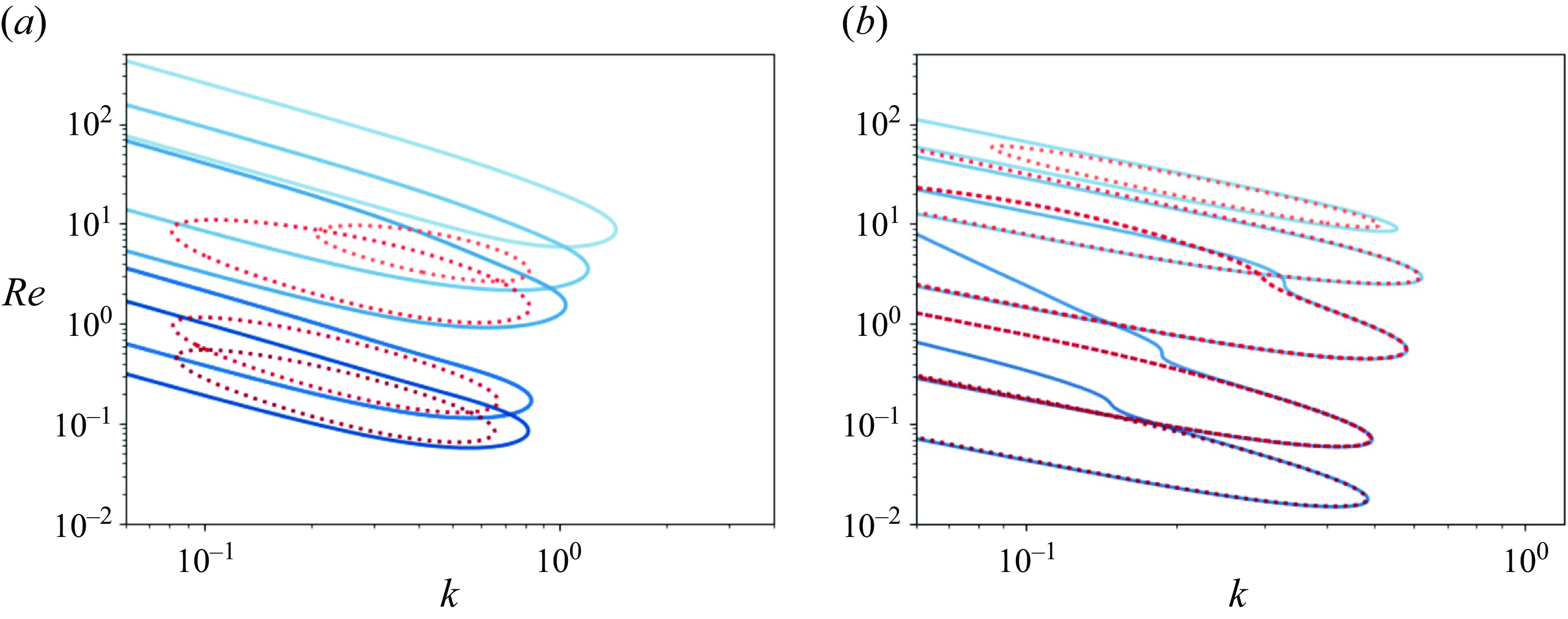
3.2. The absence of PDI
The linear stability analysis in § 3.1 was performed with $\varepsilon =0$
, and hence PDI is absent. However, to run simulations, introducing a finite
$\varepsilon =0$
, and hence PDI is absent. However, to run simulations, introducing a finite $\varepsilon$
could potentially introduce PDI, as is the case for wall-bounded flows. We check that PDI is not in this system by considering how the neutral curves in the
$\varepsilon$
could potentially introduce PDI, as is the case for wall-bounded flows. We check that PDI is not in this system by considering how the neutral curves in the $(W,k)$
plane are affected by introducing finite
$(W,k)$
plane are affected by introducing finite $\varepsilon =10^{-3}$
in figure 6. Wavenumbers up to
$\varepsilon =10^{-3}$
in figure 6. Wavenumbers up to $k=100$
were considered. The centre-mode loops that exists with vanishing
$k=100$
were considered. The centre-mode loops that exists with vanishing $\varepsilon$
are adjusted slightly, but no new modes of instability are identified, meaning PDI was not found in vKf. This was true when
$\varepsilon$
are adjusted slightly, but no new modes of instability are identified, meaning PDI was not found in vKf. This was true when $\beta =0.95$
, meaning the simulations in § 4 and 5 do not contain PDI. In addition, we checked for PDI in a more concentrated fluid (
$\beta =0.95$
, meaning the simulations in § 4 and 5 do not contain PDI. In addition, we checked for PDI in a more concentrated fluid ( $\beta =0.2$
), where PDI was demonstrated to be particularly unstable in bounded flows (Lewy & Kerswell Reference Lewy and Kerswell2024). The lack of PDI in Kolmogorov flow is consistent with Lewy & Kerswell (Reference Lewy and Kerswell2024) which considers
$\beta =0.2$
), where PDI was demonstrated to be particularly unstable in bounded flows (Lewy & Kerswell Reference Lewy and Kerswell2024). The lack of PDI in Kolmogorov flow is consistent with Lewy & Kerswell (Reference Lewy and Kerswell2024) which considers $\beta \ll 1$
and suggests that PDI requires boundaries to exist in such a fluid. This finding confirms that PDI is not necessarily seeded at regions of maximal base shear when polymer stress diffusion is present, as was the case in the wall-bounded rectilinear flows.
$\beta \ll 1$
and suggests that PDI requires boundaries to exist in such a fluid. This finding confirms that PDI is not necessarily seeded at regions of maximal base shear when polymer stress diffusion is present, as was the case in the wall-bounded rectilinear flows.
The neutral curves for non-zero-frequency modes in the $(Re, k)$
plane when
$(Re, k)$
plane when $\mu =0$
,
$\mu =0$
, $\varepsilon =0$
(blue solid lines) and finite
$\varepsilon =0$
(blue solid lines) and finite $\varepsilon =10^{-3}$
(red dotted lines) when (a)
$\varepsilon =10^{-3}$
(red dotted lines) when (a) $\beta =0.95$
and
$\beta =0.95$
and $E = 8, 16, 32, 256, 512$
(light to dark) and (b)
$E = 8, 16, 32, 256, 512$
(light to dark) and (b) $\beta =0.2$
and
$\beta =0.2$
and $E=0.5, 1, 2, 8, 64, 256$
(light to dark). Wavenumbers as high as
$E=0.5, 1, 2, 8, 64, 256$
(light to dark). Wavenumbers as high as $k=100$
were considered. These demonstrate that PDI was not identified in Kolmogorov flow, and that finite
$k=100$
were considered. These demonstrate that PDI was not identified in Kolmogorov flow, and that finite $\varepsilon$
generally stabilises the centre-mode instability.
$\varepsilon$
generally stabilises the centre-mode instability.
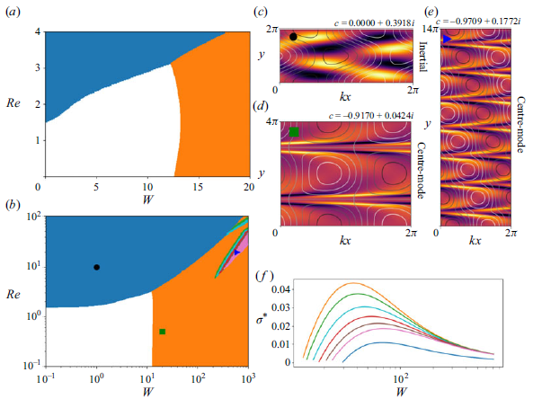
 $(a)$
The most unstable Floquet modes in the
$(a)$
The most unstable Floquet modes in the $(Re, W)$
plane for
$(Re, W)$
plane for $\beta =0.95$
, with
$\beta =0.95$
, with $\varepsilon =0$
and instabilities over wavenumbers
$\varepsilon =0$
and instabilities over wavenumbers $k \in \mathbb {R}$
are considered, with colour denoting which Floquet mode is most unstable. Colours correspond to
$k \in \mathbb {R}$
are considered, with colour denoting which Floquet mode is most unstable. Colours correspond to $\mu =0$
(blue),
$\mu =0$
(blue), $\mu =1/2$
(orange),
$\mu =1/2$
(orange), $\mu =1/3$
(green),
$\mu =1/3$
(green), $\mu =1/4$
(cyan),
$\mu =1/4$
(cyan), $\mu =1/5$
(red),
$\mu =1/5$
(red), $\mu =1/6$
(brown),
$\mu =1/6$
(brown), $\mu =1/7$
(pink).
$\mu =1/7$
(pink). $(b)$
The same on a log scale. Eigenfunctions are plotted with parameters
$(b)$
The same on a log scale. Eigenfunctions are plotted with parameters $(c)$
$(c)$ $(W, Re, k, \mu ) = (1, 10, 0.5, 0)$
,
$(W, Re, k, \mu ) = (1, 10, 0.5, 0)$
, $(d)$
$(d)$ $(W, Re, k, \mu ) = (20, 0.5, 0.5, 1/2)$
and
$(W, Re, k, \mu ) = (20, 0.5, 0.5, 1/2)$
and $(e)$
$(e)$ $(W, Re, k, \mu ) = (600, 20, 0.01, 1/7)$
.
$(W, Re, k, \mu ) = (600, 20, 0.01, 1/7)$
. $(f)$
The maximum growth rate
$(f)$
The maximum growth rate $\sigma ^*$
of each Floquet mode (same colours as in [
$\sigma ^*$
of each Floquet mode (same colours as in [ $a$
]) across all
$a$
]) across all $k\in \mathbb {R}$
for
$k\in \mathbb {R}$
for $Re=0$
,
$Re=0$
, $\beta =0.95$
and
$\beta =0.95$
and $\varepsilon =0$
as
$\varepsilon =0$
as $W$
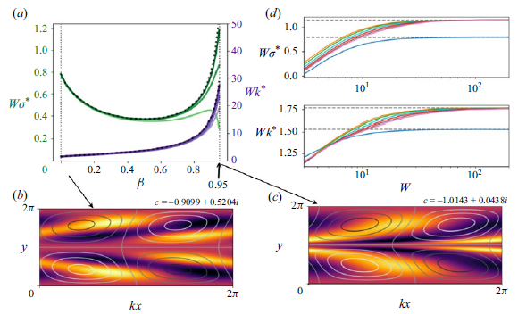
varies. These plots demonstrate that all elastic instabilities are the centre mode, which is generally most unstable when
$W$
varies. These plots demonstrate that all elastic instabilities are the centre mode, which is generally most unstable when $\mu =1/2$
, while the inertial instability is most unstable when
$\mu =1/2$
, while the inertial instability is most unstable when $\mu =0$
.
$\mu =0$
.
3.3.
Modulated disturbances (
$n\gt 1$
)

In this section we consider linear stability when $n\gt 1$
by considering modes with Floquet exponents
$n\gt 1$
by considering modes with Floquet exponents $\mu$
satisfying
$\mu$
satisfying $1/\mu \in \mathbb {N}$
. Figure 7 shows the most unstable Floquet modes in the
$1/\mu \in \mathbb {N}$
. Figure 7 shows the most unstable Floquet modes in the $(Re, W)$
plane for a viscosity ratio of
$(Re, W)$
plane for a viscosity ratio of $\beta =0.95$
. All wavenumbers
$\beta =0.95$
. All wavenumbers $k\in \mathbb {R}$
are considered, as well as the first seven Floquet modes in figures 7(a) and 7(b), which focus on the behaviour of the system at small and large
$k\in \mathbb {R}$
are considered, as well as the first seven Floquet modes in figures 7(a) and 7(b), which focus on the behaviour of the system at small and large $(Re, W)$
, respectively. The orange regions demonstrate that it is the
$(Re, W)$
, respectively. The orange regions demonstrate that it is the $\mu =1/2$
Floquet mode that generally makes the centre-mode instability most unstable, corresponding to perturbations with wavelengths of
$\mu =1/2$
Floquet mode that generally makes the centre-mode instability most unstable, corresponding to perturbations with wavelengths of $4\pi$
in the
$4\pi$
in the $y$
direction or double the forcing wavelength. These are therefore ‘subharmonic’ disturbances as they have half the spatial frequency of the forcing. The blue region shows that the inertial (Newtonian) instability is most unstable when
$y$
direction or double the forcing wavelength. These are therefore ‘subharmonic’ disturbances as they have half the spatial frequency of the forcing. The blue region shows that the inertial (Newtonian) instability is most unstable when $\mu =0$
, when there is no modulation and perturbations have the same wavelength as the forcing, i.e. ‘harmonic’ disturbances. The neutral curve in figure 7(a) resembles figure 1 in Boffetta et al. (Reference Boffetta, Celani, Mazzino, Puliafito and Vergassola2005), which considered the stability of a system equivalent to
$\mu =0$
, when there is no modulation and perturbations have the same wavelength as the forcing, i.e. ‘harmonic’ disturbances. The neutral curve in figure 7(a) resembles figure 1 in Boffetta et al. (Reference Boffetta, Celani, Mazzino, Puliafito and Vergassola2005), which considered the stability of a system equivalent to $n=64$
and
$n=64$
and $k\in \mathbb {N}/64$
. They identified the distinct elastic and inertial instabilities, but our plot allows us to in addition identify the most unstable wavelength of perturbation. It is generally the subharmonic that determines the linear stability of the centre mode. The neutral curves of figure 7(b) are zoomed out and use a log scaling which reveals that there is a part of the parameter space where even lower-order harmonics are most unstable.
$k\in \mathbb {N}/64$
. They identified the distinct elastic and inertial instabilities, but our plot allows us to in addition identify the most unstable wavelength of perturbation. It is generally the subharmonic that determines the linear stability of the centre mode. The neutral curves of figure 7(b) are zoomed out and use a log scaling which reveals that there is a part of the parameter space where even lower-order harmonics are most unstable. $(a)$
The maximum growth rate
$(a)$
The maximum growth rate $\sigma ^*$
and most unstable wavenumber
$\sigma ^*$
and most unstable wavenumber $k^*$
as
$k^*$
as $\beta$
varies when
$\beta$
varies when $Re=0$
,
$Re=0$
, $\varepsilon =0$
,
$\varepsilon =0$
, $\mu =0$
and
$\mu =0$
and $W=40, 80, 160$
(light to dark). Asymptotics derived in Appendix A are shown by the black dotted lines. Most unstable eigenfunctions are shown for
$W=40, 80, 160$
(light to dark). Asymptotics derived in Appendix A are shown by the black dotted lines. Most unstable eigenfunctions are shown for $W=160$
and (b)
$W=160$
and (b) $\beta =0$
and (c)
$\beta =0$
and (c) $\beta =0.95$
with colours showing the polymer stress trace field and contours showing the streamfunction. (
$\beta =0.95$
with colours showing the polymer stress trace field and contours showing the streamfunction. ( $d)$
Plots of
$d)$
Plots of $\sigma ^*$
and
$\sigma ^*$
and $k^*$
in the inertialess UCM fluid for various Floquet modes with
$k^*$
in the inertialess UCM fluid for various Floquet modes with $\beta =0$
,
$\beta =0$
, $Re=0$
,
$Re=0$
, $\varepsilon =0$
and
$\varepsilon =0$
and $\mu =0, 1/2, 1/3, \ldots , 1/7$
with colours as in figure 7. The asymptotic limits as
$\mu =0, 1/2, 1/3, \ldots , 1/7$
with colours as in figure 7. The asymptotic limits as $W\rightarrow \infty$
are shown by horizontal black dashed lines. When
$W\rightarrow \infty$
are shown by horizontal black dashed lines. When $\mu =0$
,
$\mu =0$
, $W\sigma ^* \rightarrow 0.784$
and
$W\sigma ^* \rightarrow 0.784$
and $Wk^* \rightarrow 1.526$
, while when
$Wk^* \rightarrow 1.526$
, while when $\mu \gt 0$
,
$\mu \gt 0$
, $W\sigma ^* \rightarrow 1.139$
and
$W\sigma ^* \rightarrow 1.139$
and $Wk^* \rightarrow 1.764$
. The centre mode is therefore generic across
$Wk^* \rightarrow 1.764$
. The centre mode is therefore generic across $\beta$
, existing even in the UCM fluid, and
$\beta$
, existing even in the UCM fluid, and $k^* \sim W^{-1}$
and
$k^* \sim W^{-1}$
and $\sigma ^* \sim W^{-1}$
.
$\sigma ^* \sim W^{-1}$
.
The $\mu =0$
inertial instability is shown in figure 7(c). Its trace field is antisymmetric about lines of peak base velocity, and it has zero frequency. The
$\mu =0$
inertial instability is shown in figure 7(c). Its trace field is antisymmetric about lines of peak base velocity, and it has zero frequency. The $\mu =1/2$
centre mode is shown in figure 7(d), and is clearly a modulated version of the
$\mu =1/2$
centre mode is shown in figure 7(d), and is clearly a modulated version of the $\mu =0$
centre mode shown in figure 5(d). Similarly, we plot the preferred mode when lower-order harmonics of the centre mode are most unstable in figure 7(e). This suggests that all elastic instabilities are centre modes for all Floquet modes, not just when
$\mu =0$
centre mode shown in figure 5(d). Similarly, we plot the preferred mode when lower-order harmonics of the centre mode are most unstable in figure 7(e). This suggests that all elastic instabilities are centre modes for all Floquet modes, not just when $\mu =0$
.
$\mu =0$
.
The dependence of the centre-mode growth rate on $\mu$
is shown in figure 7(f). We consider vanishing inertia (
$\mu$
is shown in figure 7(f). We consider vanishing inertia ( $Re=0$
), and consider the maximum growth rate across all wavenumbers,
$Re=0$
), and consider the maximum growth rate across all wavenumbers, $\sigma ^* := \max_{k \in \mathbb {R}} \sigma$
, as
$\sigma ^* := \max_{k \in \mathbb {R}} \sigma$
, as $W$
varies for fixed
$W$
varies for fixed $\mu$
(
$\mu$
( $k^*$
is defined as the most unstable wavenumber). We see that the harmonic disturbances (
$k^*$
is defined as the most unstable wavenumber). We see that the harmonic disturbances ( $\mu =0$
) are the most stable of those plotted. The subharmonic with modulation
$\mu =0$
) are the most stable of those plotted. The subharmonic with modulation $\mu =1/2$
is the most unstable, and then subsequent modulations increase in stability.
$\mu =1/2$
is the most unstable, and then subsequent modulations increase in stability.
3.4. The inertialess centre mode in the UCM fluid
So far we have mainly limited our results to the specific choice of $\beta =0.95$
. At this dilute concentration, the elastic instabilities in vKf for both
$\beta =0.95$
. At this dilute concentration, the elastic instabilities in vKf for both $n=1$
and
$n=1$
and $n\gt 1$
have been identified as the centre mode. We now demonstrate that the centre mode exists not only when
$n\gt 1$
have been identified as the centre mode. We now demonstrate that the centre mode exists not only when $\beta \sim 1$
, but for all
$\beta \sim 1$
, but for all $\beta$
. It even exists when
$\beta$
. It even exists when $\beta =0$
and the model reduces to the UCM fluid.
$\beta =0$
and the model reduces to the UCM fluid.
We plot in figure 8(a) the maximum growth rate $\sigma ^*$
and the most unstable wavenumber
$\sigma ^*$
and the most unstable wavenumber $k^*$
of the inertialess instability as
$k^*$
of the inertialess instability as $\beta$
varies for the
$\beta$
varies for the $n=1$
system. This shows that there is a smooth continuation of the centre mode at
$n=1$
system. This shows that there is a smooth continuation of the centre mode at $\beta =0.95$
to the instability seen at lower
$\beta =0.95$
to the instability seen at lower $\beta$
, suggesting that the instability seen at low
$\beta$
, suggesting that the instability seen at low $\beta$
is also the centre mode. Eigenfunctions are plotted at both
$\beta$
is also the centre mode. Eigenfunctions are plotted at both $\beta =0$
and
$\beta =0$
and $\beta =0.95$
in figures 8(b) and 8(c) and clearly resemble each other, again suggesting that the instability at
$\beta =0.95$
in figures 8(b) and 8(c) and clearly resemble each other, again suggesting that the instability at $\beta =0$
is the centre mode. The centre mode is not suppressed by low
$\beta =0$
is the centre mode. The centre mode is not suppressed by low $\beta$
in vKf.
$\beta$
in vKf.
Figure 8(d) shows the behaviour of the various Floquet modes in the inertialess UCM fluid. As $W\rightarrow \infty$
, all harmonics tend to the same growth rate that is more unstable than the
$W\rightarrow \infty$
, all harmonics tend to the same growth rate that is more unstable than the $\mu =0$
mode. Of these harmonics, the
$\mu =0$
mode. Of these harmonics, the $\mu =1/2$
mode is the most unstable, as was the case when
$\mu =1/2$
mode is the most unstable, as was the case when $\beta =0.95$
with vanishing inertia (shown in figure 7
g). The subharmonic is therefore most unstable for both high and low
$\beta =0.95$
with vanishing inertia (shown in figure 7
g). The subharmonic is therefore most unstable for both high and low $\beta$
.
$\beta$
.
These plots also demonstrate that the correct asymptotic scalings for the inertialess centre mode are $k^* \sim W^{-1}$
and
$k^* \sim W^{-1}$
and $\sigma ^* \sim W^{-1}$
as
$\sigma ^* \sim W^{-1}$
as $W\rightarrow \infty$
. This is shown across all
$W\rightarrow \infty$
. This is shown across all $\beta$
when
$\beta$
when $\mu =0$
(see figure 8
a) and various
$\mu =0$
(see figure 8
a) and various $\mu$
when
$\mu$
when $\beta =0$
(see figure 8
d). The equations governing the inertialess asymptotic limit of
$\beta =0$
(see figure 8
d). The equations governing the inertialess asymptotic limit of $W \rightarrow \infty$
are identified in Appendix A, and these asymptotics are plotted in both figures 8(a) and 8(d), showing their validity. The centre mode is therefore present in a very simple fluid when
$W \rightarrow \infty$
are identified in Appendix A, and these asymptotics are plotted in both figures 8(a) and 8(d), showing their validity. The centre mode is therefore present in a very simple fluid when $Re=\beta =\varepsilon =0$
and
$Re=\beta =\varepsilon =0$
and $W \rightarrow \infty$
, demonstrating that while elasticity is required for the instability to exist, inertia, viscosity and polymer diffusion are not.
$W \rightarrow \infty$
, demonstrating that while elasticity is required for the instability to exist, inertia, viscosity and polymer diffusion are not.
3.5.
Relaminarisation in the
$W\rightarrow \infty$
limit

Returning to the Oldroyd-B model, the flow becomes linearly stable as $W\rightarrow \infty$
for any fixed domain length. This is due to the centre mode only being unstable to a pocket of wavenumbers that scale like
$W\rightarrow \infty$
for any fixed domain length. This is due to the centre mode only being unstable to a pocket of wavenumbers that scale like $k \sim W^{-1}$
, as suggested by the asymptotic analysis performed in Appendix A. Hence, at sufficiently large
$k \sim W^{-1}$
, as suggested by the asymptotic analysis performed in Appendix A. Hence, at sufficiently large $W$
, all unstable wavelengths are longer than the channel itself, meaning the system is not susceptible to the centre-mode instability.
$W$
, all unstable wavelengths are longer than the channel itself, meaning the system is not susceptible to the centre-mode instability.
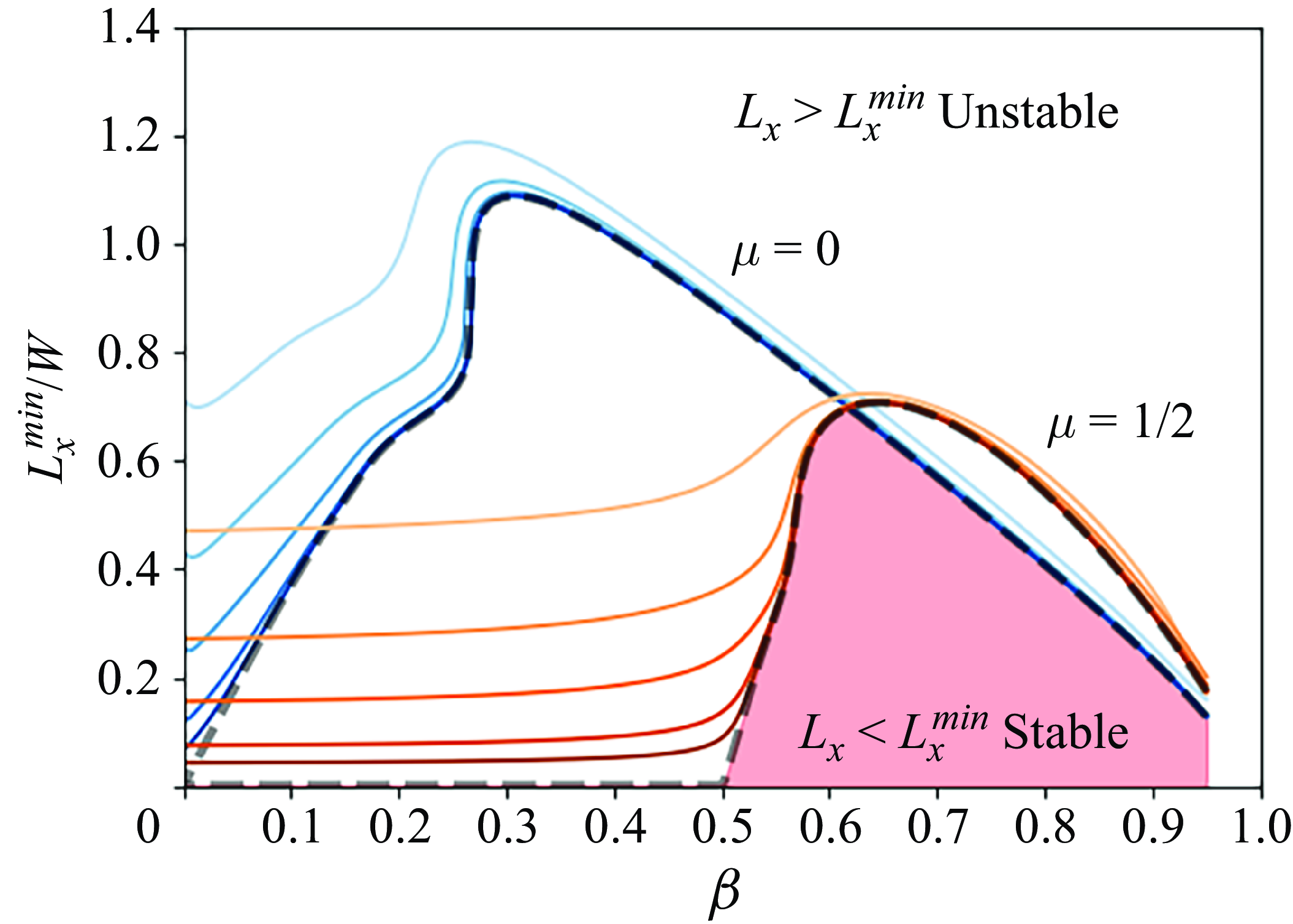
It will be useful to define $L_x^{min} := 2\pi / k_{max}$
, which is the shortest domain in which instability can be found, i.e. the system is stable when
$L_x^{min} := 2\pi / k_{max}$
, which is the shortest domain in which instability can be found, i.e. the system is stable when $L_x \lt L_x^{min}$
. When
$L_x \lt L_x^{min}$
. When $Re=0$
, figure 9 demonstrates that
$Re=0$
, figure 9 demonstrates that $L_x^{min} \sim W$
, and hence that as
$L_x^{min} \sim W$
, and hence that as $W \rightarrow \infty$
, any finite
$W \rightarrow \infty$
, any finite $L_x$
eventually becomes stable. Figure 9 also shows that the order in which the Floquet modes stabilise as
$L_x$
eventually becomes stable. Figure 9 also shows that the order in which the Floquet modes stabilise as $L_x/W \rightarrow 0$
depends on the concentration
$L_x/W \rightarrow 0$
depends on the concentration $\beta$
. This limit is achieved for fixed
$\beta$
. This limit is achieved for fixed $L_x$
as
$L_x$
as $W \rightarrow \infty$
. In this limit, when
$W \rightarrow \infty$
. In this limit, when $\beta \gt 0.62$
the
$\beta \gt 0.62$
the $\mu =1/2$
mode stabilises before the
$\mu =1/2$
mode stabilises before the $\mu =0$
mode, while the opposite is true for
$\mu =0$
mode, while the opposite is true for $\beta \lt 0.62$
. This is consistent with figure 7(f) in which
$\beta \lt 0.62$
. This is consistent with figure 7(f) in which $\beta =0.95$
, and the
$\beta =0.95$
, and the $\mu =1/2$
mode stabilises before the
$\mu =1/2$
mode stabilises before the $\mu =0$
mode for negligible inertia as
$\mu =0$
mode for negligible inertia as $W\rightarrow \infty$
. These results remain qualitatively true when inertia is introduced, with
$W\rightarrow \infty$
. These results remain qualitatively true when inertia is introduced, with $L_x^{min} \sim W$
when
$L_x^{min} \sim W$
when $Re=1, 10$
(not shown). Relaminarisation therefore occurs as
$Re=1, 10$
(not shown). Relaminarisation therefore occurs as $W\rightarrow \infty$
both with and without inertia.
$W\rightarrow \infty$
both with and without inertia.
The minimum $L_x$
at which laminar flow becomes unstable to perturbations with
$L_x$
at which laminar flow becomes unstable to perturbations with $\mu =0$
(blue) or
$\mu =0$
(blue) or $\mu =1/2$
(orange), when
$\mu =1/2$
(orange), when $Re=0$
,
$Re=0$
, $\varepsilon =0$
and
$\varepsilon =0$
and $W=50, 100, 200, 500, 1000$
(light to dark). Black dashed lines correspond to the asymptotic limit described in Appendix A, and they cross over at
$W=50, 100, 200, 500, 1000$
(light to dark). Black dashed lines correspond to the asymptotic limit described in Appendix A, and they cross over at $\beta =0.62$
. The only region which is stable as
$\beta =0.62$
. The only region which is stable as $W\rightarrow \infty$
is shaded in red. This confirms that as
$W\rightarrow \infty$
is shaded in red. This confirms that as $W \rightarrow \infty$
,
$W \rightarrow \infty$
, $L_x^{min} \sim W$
, meaning only very long channels are linearly unstable for large
$L_x^{min} \sim W$
, meaning only very long channels are linearly unstable for large $W$
. For
$W$
. For $\beta \lt 0.62$
, the
$\beta \lt 0.62$
, the $\mu =0$
harmonic stabilises before the
$\mu =0$
harmonic stabilises before the $\mu =1/2$
subharmonic as
$\mu =1/2$
subharmonic as $L_x/W\rightarrow 0$
, while the opposite is true when
$L_x/W\rightarrow 0$
, while the opposite is true when $\beta \gt 0.62$
.
$\beta \gt 0.62$
.
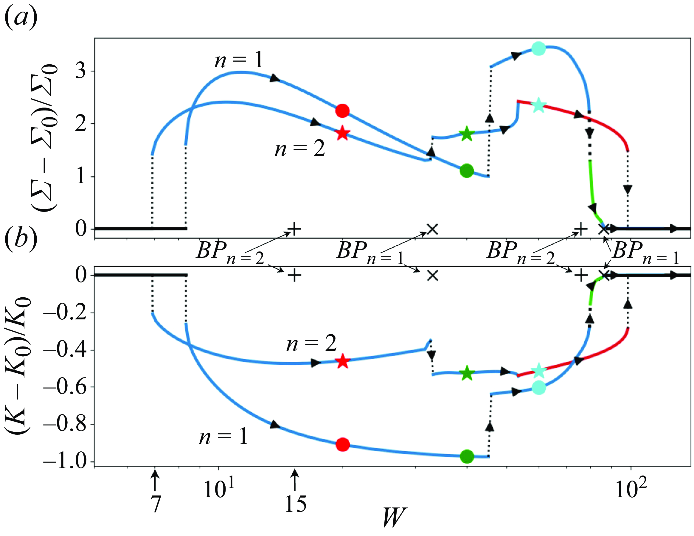
Bifurcation plots for $\beta =0.95$
,
$\beta =0.95$
, $Re=0.5$
,
$Re=0.5$
, $\varepsilon =10^{-3}$
and
$\varepsilon =10^{-3}$
and $L_x=4\pi$
. These show the deviation of the volume-averaged (a) trace
$L_x=4\pi$
. These show the deviation of the volume-averaged (a) trace $\varSigma$
and (b) kinetic energy
$\varSigma$
and (b) kinetic energy $K$
from the laminar state, which has trace and kinetic energy
$K$
from the laminar state, which has trace and kinetic energy $\varSigma _0$
and
$\varSigma _0$
and $K_0$
. We show stable solutions in both the
$K_0$
. We show stable solutions in both the $n=2$
system and the
$n=2$
system and the $n=1$
system. Blue corresponds to travelling-wave solutions, red to equilibria and green to limit cycles. The polymer stress trace of the solution at each of the six symbols are shown in figure 12. Bifurcation points (BP) due to the linear instability are shown with black crosses at
$n=1$
system. Blue corresponds to travelling-wave solutions, red to equilibria and green to limit cycles. The polymer stress trace of the solution at each of the six symbols are shown in figure 12. Bifurcation points (BP) due to the linear instability are shown with black crosses at $W=33, 86$
when
$W=33, 86$
when $n=1$
and black pluses at
$n=1$
and black pluses at $W=15, 76$
when
$W=15, 76$
when $n=2$
.
$n=2$
.
4. Subcriticality and exact coherent structures
Subcritical behaviour can be seen in the centre mode in a channel (Buza et al. Reference Buza, Beneitez, Page and Kerswell2022a
,Reference Buza, Page and Kerswell
b
) and a pipe (Wan et al. Reference Wan, Sun and Zhang2021). In this section we demonstrate that the same is also true in Kolmogorov flow. We identify the structures on the upper branch for both $n=1$
and
$n=1$
and $n=2$
, and find other stable exact coherent structures on a number of solution branches. The presence of an elastic travelling wave was first described by Berti & Boffetta (Reference Berti and Boffetta2010) in a system equivalent to
$n=2$
, and find other stable exact coherent structures on a number of solution branches. The presence of an elastic travelling wave was first described by Berti & Boffetta (Reference Berti and Boffetta2010) in a system equivalent to $L_x=L_y=8\pi$
(i.e.
$L_x=L_y=8\pi$
(i.e. $n=4$
), and we expand upon this by identifying a number of distinct elastic waves and equilibria in a simpler system with
$n=4$
), and we expand upon this by identifying a number of distinct elastic waves and equilibria in a simpler system with $L_x=L_y=4\pi$
(i.e.
$L_x=L_y=4\pi$
(i.e. $n=2$
). No chaotic behaviour was identified here, and so while our choice of parameters produces a number of different solutions, it is simple to track the solutions as we change
$n=2$
). No chaotic behaviour was identified here, and so while our choice of parameters produces a number of different solutions, it is simple to track the solutions as we change $W$
. We will later increase
$W$
. We will later increase $L_x$
from this value, which allows the system to become chaotic.
$L_x$
from this value, which allows the system to become chaotic.
We consider the bifurcation plot of the centre-mode instability in figure 10. To produce this plot we begin with laminar flow at a value of $W$
that is linearly unstable, and then add white noise and allow the system to reach its stable final state. The value of
$W$
that is linearly unstable, and then add white noise and allow the system to reach its stable final state. The value of $W$
is then adiabatically decreased until a saddle node is identified. From this saddle node,
$W$
is then adiabatically decreased until a saddle node is identified. From this saddle node, $W$
is then increased adiabatically, and the resultant stable branch of the bifurcation diagram is plotted in figure 10. This procedure was followed for both
$W$
is then increased adiabatically, and the resultant stable branch of the bifurcation diagram is plotted in figure 10. This procedure was followed for both $n=1$
and
$n=1$
and $n=2$
. The solutions on the
$n=2$
. The solutions on the $n=1$
branch can be used to construct a solution branch when
$n=1$
branch can be used to construct a solution branch when $n=2$
by repeating all fields twice in the y direction; however, the stability of this constructed branch may be different in the
$n=2$
by repeating all fields twice in the y direction; however, the stability of this constructed branch may be different in the $n=2$
system. In fact, for
$n=2$
system. In fact, for $W=20,40, 60$
the solutions constructed from the
$W=20,40, 60$
the solutions constructed from the $n=1$
branch are unstable in the
$n=1$
branch are unstable in the $n=2$
system (not shown). We plot the mean kinetic energy
$n=2$
system (not shown). We plot the mean kinetic energy $K = \langle |\mathbf {u}|^2 \rangle _V/ 2$
and the mean trace
$K = \langle |\mathbf {u}|^2 \rangle _V/ 2$
and the mean trace $\varSigma = \langle \tau _{xx} + \tau _{yy} \rangle _V$
of the solution branches, where
$\varSigma = \langle \tau _{xx} + \tau _{yy} \rangle _V$
of the solution branches, where $\langle \cdot \rangle _V$
denotes an average over the domain. Both metrics are normalised using their values in the laminar flow,
$\langle \cdot \rangle _V$
denotes an average over the domain. Both metrics are normalised using their values in the laminar flow, $\varSigma _0$
and
$\varSigma _0$
and $K_0$
. This bifurcation plot consists of a number of different branches, all of which are either laminar (black), travelling waves (blue), equilibria (red) or periodic orbits (green). For the chosen parameters of
$K_0$
. This bifurcation plot consists of a number of different branches, all of which are either laminar (black), travelling waves (blue), equilibria (red) or periodic orbits (green). For the chosen parameters of $L_x=4\pi$
with
$L_x=4\pi$
with $n=1$
or
$n=1$
or $n=2$
, no chaotic behaviour was identified.
$n=2$
, no chaotic behaviour was identified.
This plot shows that there is a saddle-node bifurcation marking the smallest $W$
at which the system is unstable to finite-amplitude disturbances, demonstrating subcriticality. We illustrate in figure 11 how this impacts the stability of vKf by plotting a neutral curve for the system that shows regions of linear instability, as well as a hatched region corresponding to where the system is subcritical. This shows that the elastic system becomes unstable to finite-amplitude perturbations at
$W$
at which the system is unstable to finite-amplitude disturbances, demonstrating subcriticality. We illustrate in figure 11 how this impacts the stability of vKf by plotting a neutral curve for the system that shows regions of linear instability, as well as a hatched region corresponding to where the system is subcritical. This shows that the elastic system becomes unstable to finite-amplitude perturbations at $W \approx 7$
, and becomes linearly unstable at
$W \approx 7$
, and becomes linearly unstable at $W \approx 15$
. The bifurcation plot in figure 10 shows that at large
$W \approx 15$
. The bifurcation plot in figure 10 shows that at large $W$
, the solutions eventually merge with the laminar state, rather than sustaining any instability. This is consistent with the relaminarisation discussed in § 3.5, which showed how the laminar state is linearly stable for sufficiently large
$W$
, the solutions eventually merge with the laminar state, rather than sustaining any instability. This is consistent with the relaminarisation discussed in § 3.5, which showed how the laminar state is linearly stable for sufficiently large $W$
.
$W$
.
The most unstable Floquet modes in the $(Re, W)$
plane for
$(Re, W)$
plane for $\beta =0.95$
,
$\beta =0.95$
, $\varepsilon =10^{-3}$
, with instabilities over wavenumbers
$\varepsilon =10^{-3}$
, with instabilities over wavenumbers $k \in \mathbb {N}/2$
considered and Floquet modes
$k \in \mathbb {N}/2$
considered and Floquet modes $\mu =0$
(blue) and
$\mu =0$
(blue) and $\mu =1/2$
(orange). The solid colours therefore show the linear stability of a simulation with
$\mu =1/2$
(orange). The solid colours therefore show the linear stability of a simulation with $n=2$
and
$n=2$
and $L_x=4\pi$
. The orange hatched region corresponds to areas in which the centre mode in this geometry has been shown to be subcritical. For
$L_x=4\pi$
. The orange hatched region corresponds to areas in which the centre mode in this geometry has been shown to be subcritical. For $Re\lt \lt 1$
, we see that the system is unstable to finite-amplitude perturbations at
$Re\lt \lt 1$
, we see that the system is unstable to finite-amplitude perturbations at $W\approx 7$
but to infinitesimal perturbations at
$W\approx 7$
but to infinitesimal perturbations at $W\approx 15$
.
$W\approx 15$
.
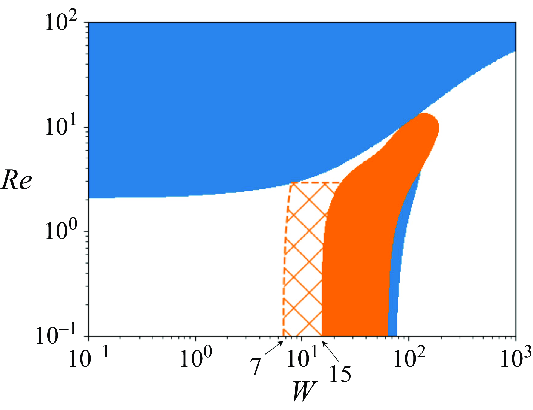
The trace fields of these solution branches at $W=20,40,60$
(all marked by symbols on the bifurcation diagram) are shown on the left-hand side of figure 12. While these solution branches all represent an attractor of the system, we note that they are not generically the final state for any initial condition. We plot the final states reached when the system is initialised with laminar flow and low-amplitude white noise on the right-hand side of figure 12. This protocol produced final states that were different from the solutions found in the bifurcation plot at
$W=20,40,60$
(all marked by symbols on the bifurcation diagram) are shown on the left-hand side of figure 12. While these solution branches all represent an attractor of the system, we note that they are not generically the final state for any initial condition. We plot the final states reached when the system is initialised with laminar flow and low-amplitude white noise on the right-hand side of figure 12. This protocol produced final states that were different from the solutions found in the bifurcation plot at $W=20,40,60$
for
$W=20,40,60$
for $n=2$
and at
$n=2$
and at $W=20,40$
for
$W=20,40$
for $n=1$
. This suggests that the basin of attraction for the identified branches in figure 10 is small. In all cases, a resolution of at least
$n=1$
. This suggests that the basin of attraction for the identified branches in figure 10 is small. In all cases, a resolution of at least $64$
modes per
$64$
modes per $2\pi$
in either
$2\pi$
in either $x$
or
$x$
or $y$
direction was used. Doubling the resolution in each direction did not qualitatively change any of the final states of figure 12.
$y$
direction was used. Doubling the resolution in each direction did not qualitatively change any of the final states of figure 12.
Many of the identified exact coherent structures share the arrowhead as a common feature, as was the case with the elastic wave found in Berti & Boffetta (Reference Berti and Boffetta2010). Generally this arrowhead moves in the direction in which the arrow points; however, this is not always true – the travelling waves on the solution branch seen when $n=2$
for
$n=2$
for $W=20$
and
$W=20$
and $W=40$
move in the opposite direction to what one might expect.
$W=40$
move in the opposite direction to what one might expect.
The trace $T_{xx} + T_{yy}$
of final states for
$T_{xx} + T_{yy}$
of final states for $\beta =0.95$
,
$\beta =0.95$
, $Re=0.5$
,
$Re=0.5$
, $\varepsilon =10^{-3}$
and
$\varepsilon =10^{-3}$
and $n=1,2$
. The left-hand column corresponds to solutions on the branches shown in the bifurcation plot in figure 10, while the right-hand column shows final states reached when the system is initialised with laminar flow and low-amplitude white noise. The wave speeds
$n=1,2$
. The left-hand column corresponds to solutions on the branches shown in the bifurcation plot in figure 10, while the right-hand column shows final states reached when the system is initialised with laminar flow and low-amplitude white noise. The wave speeds $c$
of all but one solution is shown, identifying which states are equilibria or travelling waves. For
$c$
of all but one solution is shown, identifying which states are equilibria or travelling waves. For $n=2$
,
$n=2$
, $W=20$
the white-noise-initialised solution is a relative periodic orbit (RPO), and so has no wave speed.
$W=20$
the white-noise-initialised solution is a relative periodic orbit (RPO), and so has no wave speed.
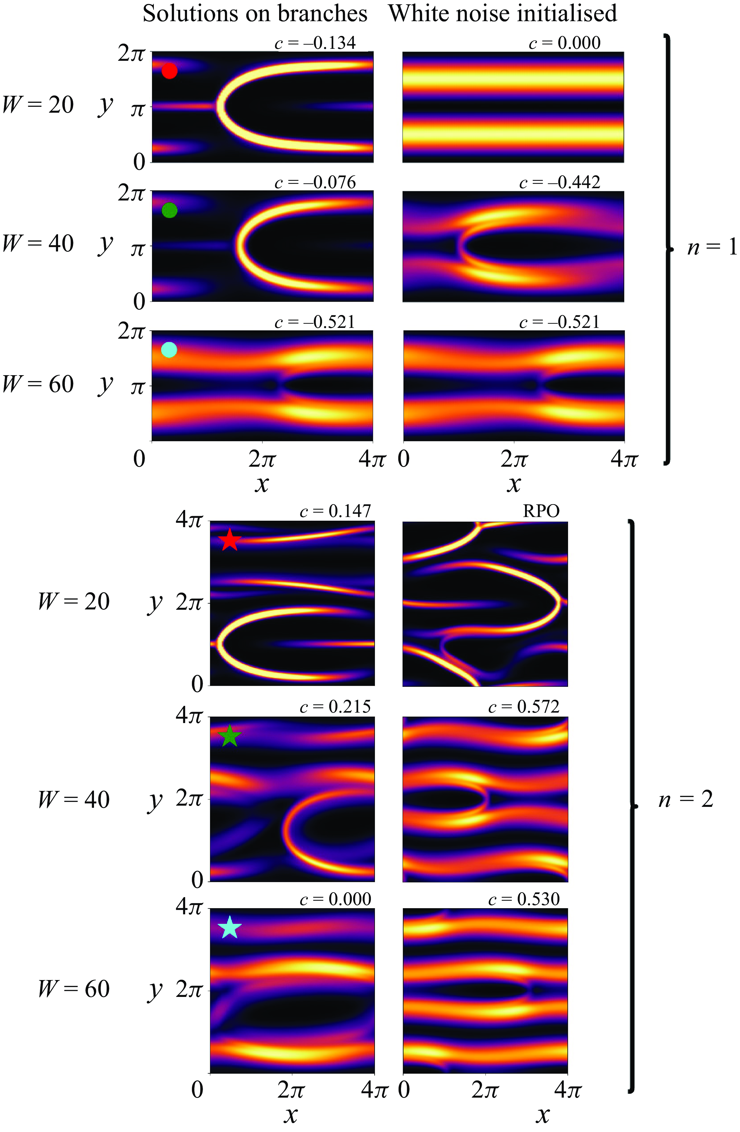
 $(a)$
State diagram of the final states identified when
$(a)$
State diagram of the final states identified when $\beta =0.95$
,
$\beta =0.95$
, $Re=0.5$
,
$Re=0.5$
, $\varepsilon =10^{-3}$
and
$\varepsilon =10^{-3}$
and $L_y=4\pi$
. For each parameter setting, we simulated the fluid initialised with random finite-amplitude disturbances (see main text for the protocol). States seen are laminar (blue circle), travelling waves (green square), periodic orbit (yellow cross), quasi-periodic orbit (black triangle) and chaos (purple star). Dashed black line shows the smallest
$L_y=4\pi$
. For each parameter setting, we simulated the fluid initialised with random finite-amplitude disturbances (see main text for the protocol). States seen are laminar (blue circle), travelling waves (green square), periodic orbit (yellow cross), quasi-periodic orbit (black triangle) and chaos (purple star). Dashed black line shows the smallest $L_x$
at which linear instability exists. On the low-shear boundary, it is the
$L_x$
at which linear instability exists. On the low-shear boundary, it is the $\mu =1/2$
Floquet mode that is marginally linearly unstable, while on the high-shear boundary it is the
$\mu =1/2$
Floquet mode that is marginally linearly unstable, while on the high-shear boundary it is the $\mu =0$
mode. Dashed red line shows the boundary of where the flow is known to be subcritical when
$\mu =0$
mode. Dashed red line shows the boundary of where the flow is known to be subcritical when $L_x=4 \pi$
as per figure 10.
$L_x=4 \pi$
as per figure 10. $(b)$
All distinct non-laminar final states identified, marked with a symbol denoting the type of state as in
$(b)$
All distinct non-laminar final states identified, marked with a symbol denoting the type of state as in $(a)$
. This plot demonstrates that instabilities have only been identified close to regions of parameter space in which the centre mode is linearly unstable, and many of these states contain an arrowhead. This suggests all non-laminar states originate from the centre-mode linear instability.
$(a)$
. This plot demonstrates that instabilities have only been identified close to regions of parameter space in which the centre mode is linearly unstable, and many of these states contain an arrowhead. This suggests all non-laminar states originate from the centre-mode linear instability.
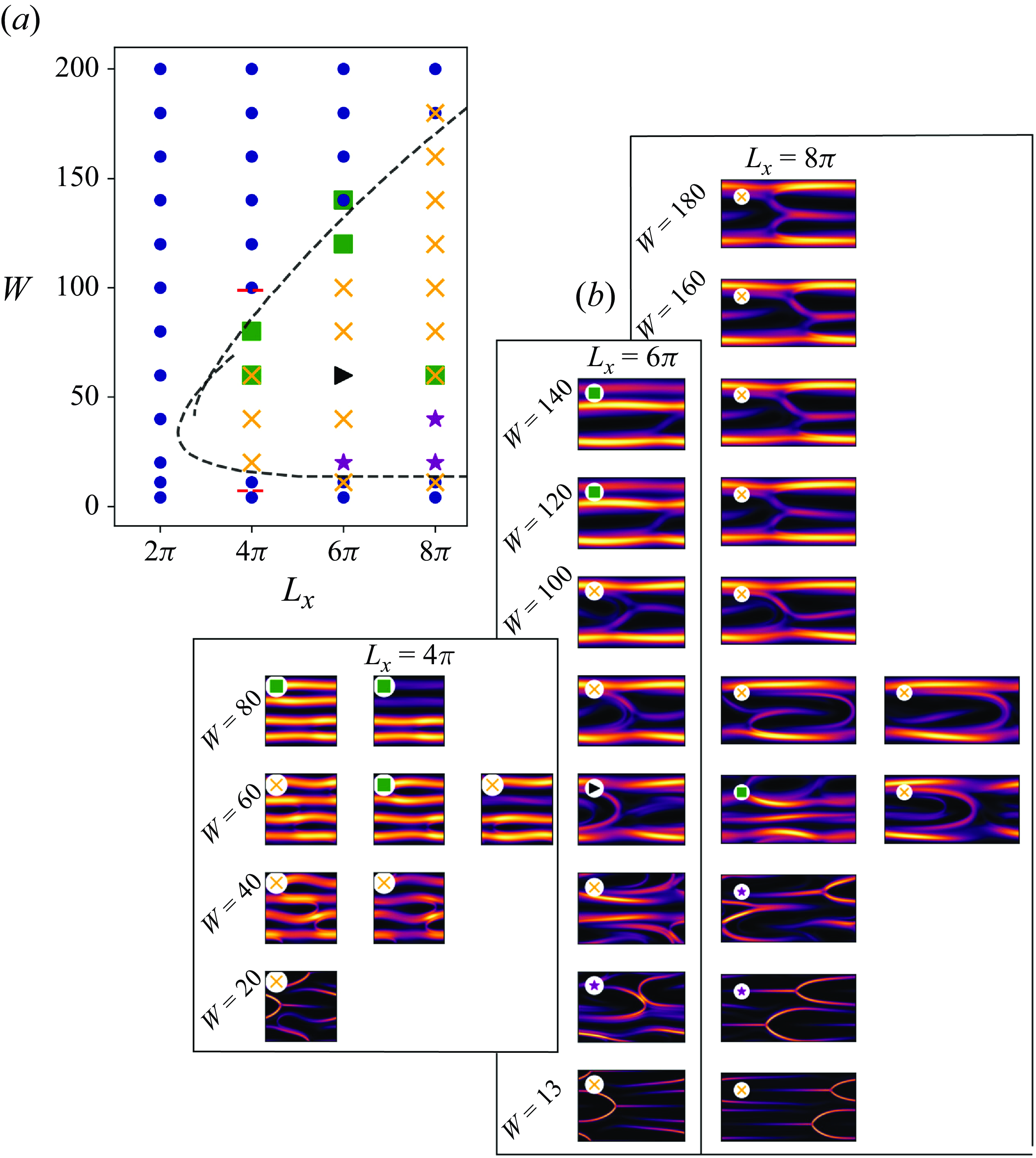
5. Elastic turbulence
So far we have examined a number of solutions in the Kolmogorov system when $L_x=L_y=4\pi$
, none of which were chaotic. We now change our domain length
$L_x=L_y=4\pi$
, none of which were chaotic. We now change our domain length $L_x$
to see how this can introduce chaos into the system. Elastic turbulence has been identified in vKf in systems equivalent to
$L_x$
to see how this can introduce chaos into the system. Elastic turbulence has been identified in vKf in systems equivalent to $L_y=8\pi$
(Berti et al. Reference Berti, Bistagnino, Boffetta, Celani and Musacchio2008), and on increasing
$L_y=8\pi$
(Berti et al. Reference Berti, Bistagnino, Boffetta, Celani and Musacchio2008), and on increasing $W$
the final state can transition from a travelling wave to a periodic state and then onto something chaotic (Berti & Boffetta Reference Berti and Boffetta2010). Berti et al. (Reference Berti, Bistagnino, Boffetta, Celani and Musacchio2008) comment on the presence of ‘wavy patterns’ in the turbulence that are made up of ‘filamental structures’. Our results indicate that the centre-mode instability is responsible for this turbulence with these structures corresponding to unstable arrowheads.
$W$
the final state can transition from a travelling wave to a periodic state and then onto something chaotic (Berti & Boffetta Reference Berti and Boffetta2010). Berti et al. (Reference Berti, Bistagnino, Boffetta, Celani and Musacchio2008) comment on the presence of ‘wavy patterns’ in the turbulence that are made up of ‘filamental structures’. Our results indicate that the centre-mode instability is responsible for this turbulence with these structures corresponding to unstable arrowheads.
5.1. The centre mode is responsible for transition to turbulence
Motivated by the presence of the centre-mode arrowhead in many of the coherent structures in § 4, we now demonstrate that the centre-mode instability is the cause of turbulence in this system. In fact, in the absence of any other elastic instabilities, all the dynamics ultimately comes from the centre-mode instability.
We first produce a state diagram in figure 13(a), which shows what types of final states are reached when simulations are initialised with finite-amplitude disturbances as the Weissenberg number $W$
and channel length
$W$
and channel length $L_x$
are varied. Each state was found by taking the laminar base flow and adding a random perturbation to the first 50 % of the Fourier modes in fields
$L_x$
are varied. Each state was found by taking the laminar base flow and adding a random perturbation to the first 50 % of the Fourier modes in fields $u$
,
$u$
, $T_{xx}$
and
$T_{xx}$
and $T_{xy}$
, with an amplitude of 10 % of the mean laminar base field. All remaining initial fields were constructed from these. We simulated each pair of parameters (
$T_{xy}$
, with an amplitude of 10 % of the mean laminar base field. All remaining initial fields were constructed from these. We simulated each pair of parameters ( $W$
,
$W$
, $L_x$
) five times, and identify the final states as either laminar (blue circle), a travelling wave (green square), a periodic orbit (yellow cross), a quasi-periodic orbit (black triangle) or chaotic (purple star) using the procedure discussed in Appendix B. In regions of linear stability, this protocol produced exclusively laminar solutions, so to demonstrate subcriticality we simulated an additional 10 runs as well. In these, random perturbations were added to the first 5 % of Fourier modes with an amplitude of 20 % of the laminar base field for five runs, and an amplitude of 10 % of the laminar base field was set in the other five. This focus on longer-wavelength perturbations was sufficient to excite subcritical solutions; however, not all subcritical solutions were found, as a subcritical travelling-wave solution that is known to exist at
$L_x$
) five times, and identify the final states as either laminar (blue circle), a travelling wave (green square), a periodic orbit (yellow cross), a quasi-periodic orbit (black triangle) or chaotic (purple star) using the procedure discussed in Appendix B. In regions of linear stability, this protocol produced exclusively laminar solutions, so to demonstrate subcriticality we simulated an additional 10 runs as well. In these, random perturbations were added to the first 5 % of Fourier modes with an amplitude of 20 % of the laminar base field for five runs, and an amplitude of 10 % of the laminar base field was set in the other five. This focus on longer-wavelength perturbations was sufficient to excite subcritical solutions; however, not all subcritical solutions were found, as a subcritical travelling-wave solution that is known to exist at $W=13, L_x=4\pi$
(see figure 10) was not found here. For some parameters these runs identified multiple types of final states, which are indicated as overlaid symbols in figure 13. These simulations used a resolution of
$W=13, L_x=4\pi$
(see figure 10) was not found here. For some parameters these runs identified multiple types of final states, which are indicated as overlaid symbols in figure 13. These simulations used a resolution of $(N_x, N_y)=(128, 192)$
Fourier modes with a time step of
$(N_x, N_y)=(128, 192)$
Fourier modes with a time step of $\textrm{d}t=8\times 10^{-3}$
and were confirmed using
$\textrm{d}t=8\times 10^{-3}$
and were confirmed using $(N_x, N_y)=(256, 256)$
.
$(N_x, N_y)=(256, 256)$
.
Non-laminar solutions were only seen in regions of parameter space close to where the centre mode is linearly unstable, suggesting that these states originate from the centre-mode bifurcation. We plot all distinct final states in figure 13(b). While some states look similar (e.g. those at $W=80$
,
$W=80$
, $L_x=8\pi$
), kinetic energy time series differ (not shown).
$L_x=8\pi$
), kinetic energy time series differ (not shown).
For the parameters considered, the shortest channel in which chaotic behaviour was found was $L_x=6\pi$
, at
$L_x=6\pi$
, at $W$
corresponding to the low-shear region of where the centre mode is linearly unstable. To check that the chaos was self-sustaining and not transient, we ran all chaotic simulations for
$W$
corresponding to the low-shear region of where the centre mode is linearly unstable. To check that the chaos was self-sustaining and not transient, we ran all chaotic simulations for $10^5$
time units of
$10^5$
time units of $2\pi U_0 / L_0$
, and saw no collapse in the time series of
$2\pi U_0 / L_0$
, and saw no collapse in the time series of $K$
.
$K$
.
To examine the transition scenario, the turbulent state at $W=20$
and
$W=20$
and $L_x=6\pi$
was taken as a starting point and then
$L_x=6\pi$
was taken as a starting point and then $W$
lowered adiabatically. Figure 14 shows how the flow transitions from one where the time series of
$W$
lowered adiabatically. Figure 14 shows how the flow transitions from one where the time series of $K$
is chaotic to one that is periodic via regions of quasi-periodicity as
$K$
is chaotic to one that is periodic via regions of quasi-periodicity as $W$
is decreased, before eventually becoming a constant when the state is a travelling wave. At
$W$
is decreased, before eventually becoming a constant when the state is a travelling wave. At $W=18$
, the onset of turbulence is marked by the presence of bursting events that temporarily increase
$W=18$
, the onset of turbulence is marked by the presence of bursting events that temporarily increase $K$
seemingly at random, before returning to periodic behaviour. When
$K$
seemingly at random, before returning to periodic behaviour. When $W$
is decreased further, periodic behaviour (e.g. at
$W$
is decreased further, periodic behaviour (e.g. at $W=17$
) and quasi-periodicity (e.g. at
$W=17$
) and quasi-periodicity (e.g. at $W=15$
) are found, until a travelling-wave state is realised at
$W=15$
) are found, until a travelling-wave state is realised at $W=7$
. The periodic and travelling-wave solutions closely resemble the centre-mode arrowhead.
$W=7$
. The periodic and travelling-wave solutions closely resemble the centre-mode arrowhead.
Kinetic energy time series of solutions (left), with the trace field at $t=5000$
(right) as
$t=5000$
(right) as $W$
is lowered from
$W$
is lowered from $W=20$
. The trace field colours use the same scale as figure 18 for comparison purposes. Parameters are
$W=20$
. The trace field colours use the same scale as figure 18 for comparison purposes. Parameters are $\beta =0.95$
,
$\beta =0.95$
, $Re=0.5$
,
$Re=0.5$
, $\varepsilon =10^{-3}$
,
$\varepsilon =10^{-3}$
, $n=2$
and
$n=2$
and $L_x=6\pi$
. Symbols, as in figure 13(a), show chaos (purple star), quasi-periodic orbits (black triangle), periodic orbit (yellow cross) and a travelling wave (green square). This shows that the turbulent state at
$L_x=6\pi$
. Symbols, as in figure 13(a), show chaos (purple star), quasi-periodic orbits (black triangle), periodic orbit (yellow cross) and a travelling wave (green square). This shows that the turbulent state at $W=20$
is connected to states that strongly resemble the centre-mode arrowhead.
$W=20$
is connected to states that strongly resemble the centre-mode arrowhead.
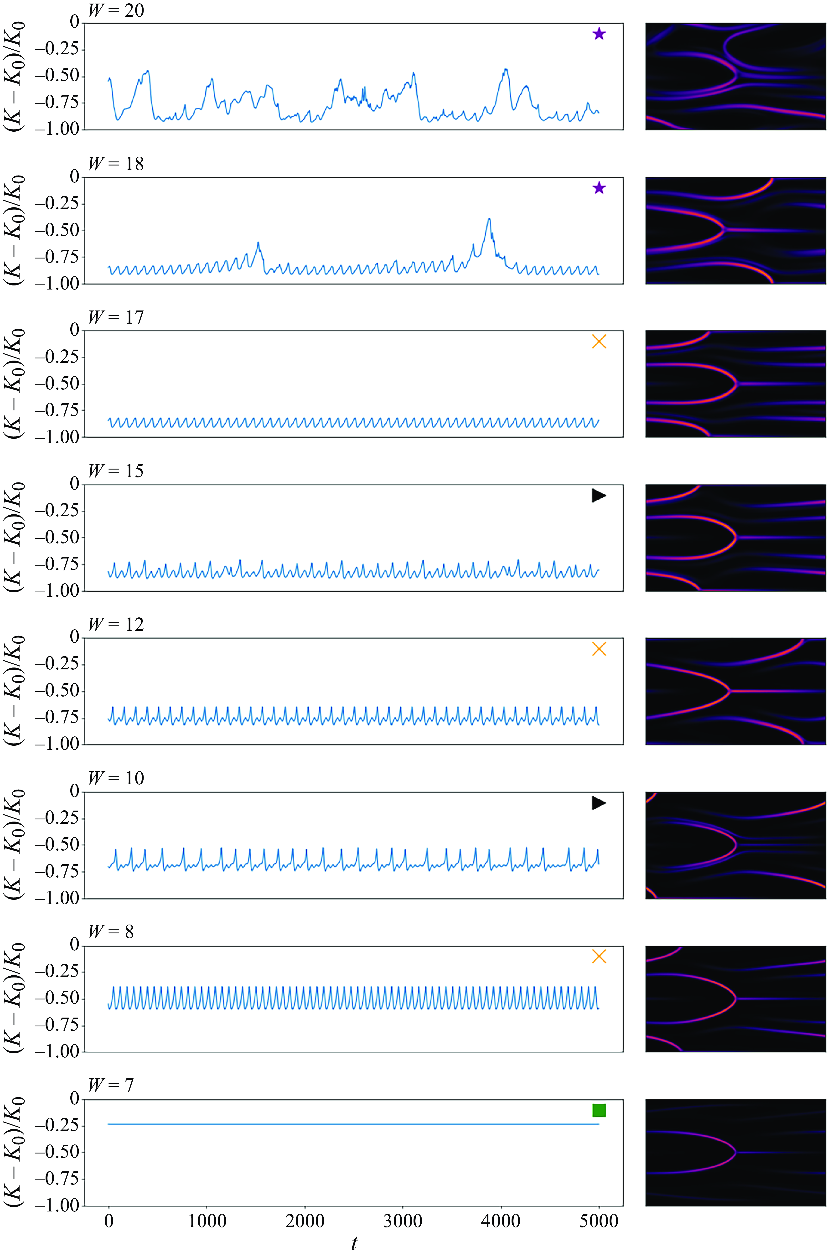
Power spectra for the states from figure 14 with $W=15$
and
$W=15$
and $W=10$
. This shows that the state at
$W=10$
. This shows that the state at $W=15$
is truly a quasi-periodic orbit with discrete incommensurate frequencies, while the state at
$W=15$
is truly a quasi-periodic orbit with discrete incommensurate frequencies, while the state at $W=10$
has a broad band of frequencies.
$W=10$
has a broad band of frequencies.
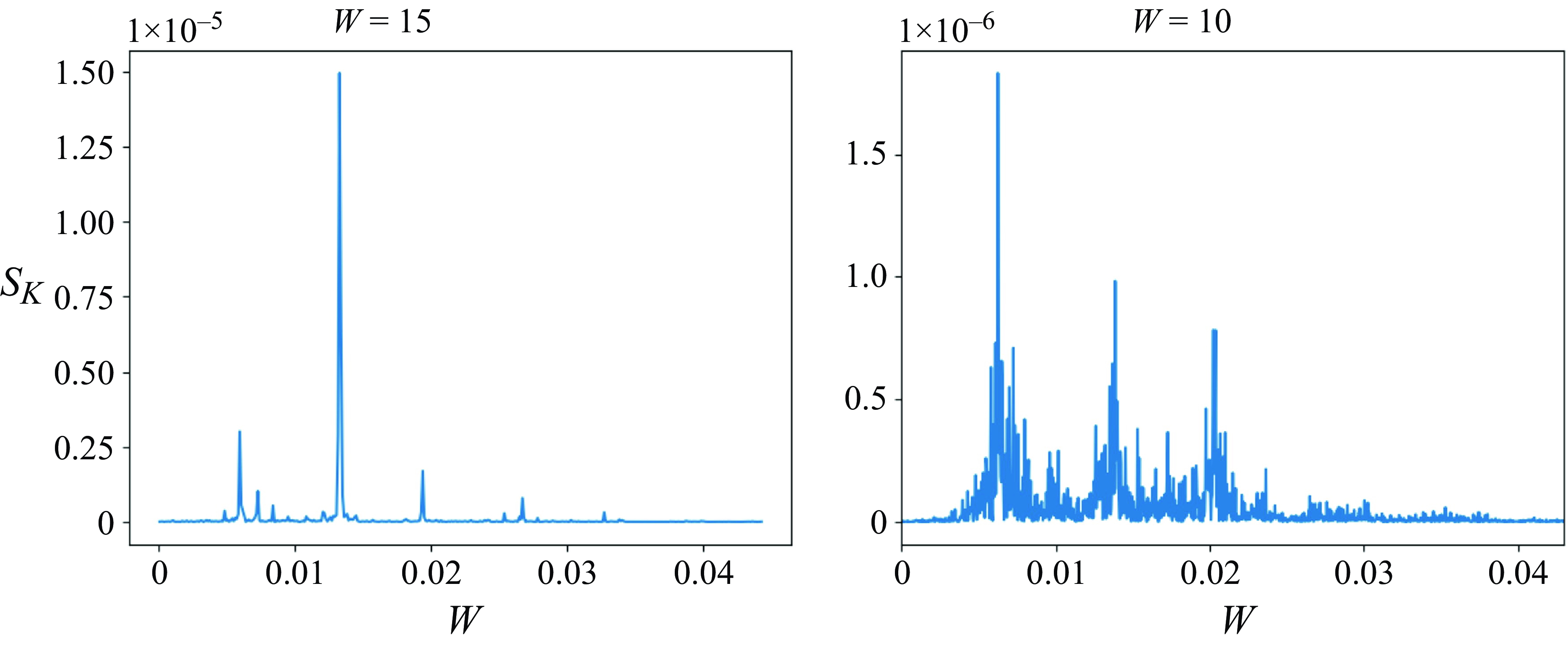
We plot the frequency spectra of the quasi-periodic behaviour at $W=15$
and
$W=15$
and $W=10$
in figure 15, where
$W=10$
in figure 15, where
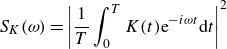 \begin{align} S_K(\omega ) = \left |\frac {1}{T} \int _0^TK(t)\textrm{e}^{-i\omega t} \textrm{d}t\right |^2 \end{align}
is the Fourier transform of the kinetic energy $K$
over a long time
$K$
over a long time $T=50\,000$
. While
$T=50\,000$
. While $W=15$
clearly shows discrete incommensurate frequencies,
$W=15$
clearly shows discrete incommensurate frequencies, $W=10$
shows a low-level broad band of frequencies. We still describe the latter as quasi-periodic, however, as it contains a small number of dominant frequencies that are incommensurate. Figure 14 used
$W=10$
shows a low-level broad band of frequencies. We still describe the latter as quasi-periodic, however, as it contains a small number of dominant frequencies that are incommensurate. Figure 14 used $\varepsilon =10^{-3}$
, and was run with a resolution of
$\varepsilon =10^{-3}$
, and was run with a resolution of $(N_x, N_y) = (196, 128)$
. The results were robust to a doubling of the resolution in both directions. In addition, we checked that
$(N_x, N_y) = (196, 128)$
. The results were robust to a doubling of the resolution in both directions. In addition, we checked that $\varepsilon =10^{-4}$
ran at
$\varepsilon =10^{-4}$
ran at $(N_x, N_y) = (384, 384)$
produced qualitatively similar results, despite the arrowheads being thinner (see Appendix C). The bursting scenario is still identifiable.
$(N_x, N_y) = (384, 384)$
produced qualitatively similar results, despite the arrowheads being thinner (see Appendix C). The bursting scenario is still identifiable.
Finally, it is worth remarking that the transition scenario identified here is not the only one possible in vKf. In the regime discussed with $n=2$
and
$n=2$
and $L_x=6\pi$
, a bifurcation triggers irregular bursting events that become more frequent with increasing
$L_x=6\pi$
, a bifurcation triggers irregular bursting events that become more frequent with increasing $W$
. Elastic turbulence is then seen above a critical
$W$
. Elastic turbulence is then seen above a critical $W$
where the disordered state exists at all times. An alternative transition to turbulence has been recently identified when
$W$
where the disordered state exists at all times. An alternative transition to turbulence has been recently identified when $n=1$
and
$n=1$
and $L_x=8\pi$
, in which a sequence of period-doubling bifurcations cascade into turbulence (Nichols, Guy & Thomases Reference Nichols, Guy and Thomases2024).
$L_x=8\pi$
, in which a sequence of period-doubling bifurcations cascade into turbulence (Nichols, Guy & Thomases Reference Nichols, Guy and Thomases2024). $(a, b)$
Simulations when
$(a, b)$
Simulations when $W=15$
(periodic, blue),
$W=15$
(periodic, blue), $W=20$
(low-dimensional chaos, orange) and
$W=20$
(low-dimensional chaos, orange) and $W=30$
(turbulent, green), with rows of
$W=30$
(turbulent, green), with rows of $(a)$
showing the trace field evolving over time, with times marked on the time series of
$(a)$
showing the trace field evolving over time, with times marked on the time series of $K$
in
$K$
in $(b)$
.
$(b)$
. $(c)$
The compensated power spectra for
$(c)$
The compensated power spectra for $W=15$
(blue),
$W=15$
(blue), $20$
(orange),
$20$
(orange), $30$
(green),
$30$
(green), $40$
(red),
$40$
(red), $50$
(purple), suggesting a regime where
$50$
(purple), suggesting a regime where $E_K \sim k^{-4}$
, with regular spectra shown in the inset.
$E_K \sim k^{-4}$
, with regular spectra shown in the inset. $(d)$
Contributions to the kinetic energy due to the base shear (
$(d)$
Contributions to the kinetic energy due to the base shear ( $\mathcal {P}$
), elastic forces (
$\mathcal {P}$
), elastic forces ( $\mathcal {E}_{elast}$
) and viscous forces (
$\mathcal {E}_{elast}$
) and viscous forces ( $\mathcal {E}_{visc}$
) as
$\mathcal {E}_{visc}$
) as $W$
varies. Each quantity is averaged over a long time (
$W$
varies. Each quantity is averaged over a long time ( $T=20\,000$
), with error bars showing plus and minus one standard deviation. Other parameters are
$T=20\,000$
), with error bars showing plus and minus one standard deviation. Other parameters are $\beta =0.95$
,
$\beta =0.95$
, $Re=0.5$
,
$Re=0.5$
, $\varepsilon =10^{-3}$
,
$\varepsilon =10^{-3}$
, $n=2$
and
$n=2$
and $L_x=8\pi$
in all plots.
$L_x=8\pi$
in all plots.
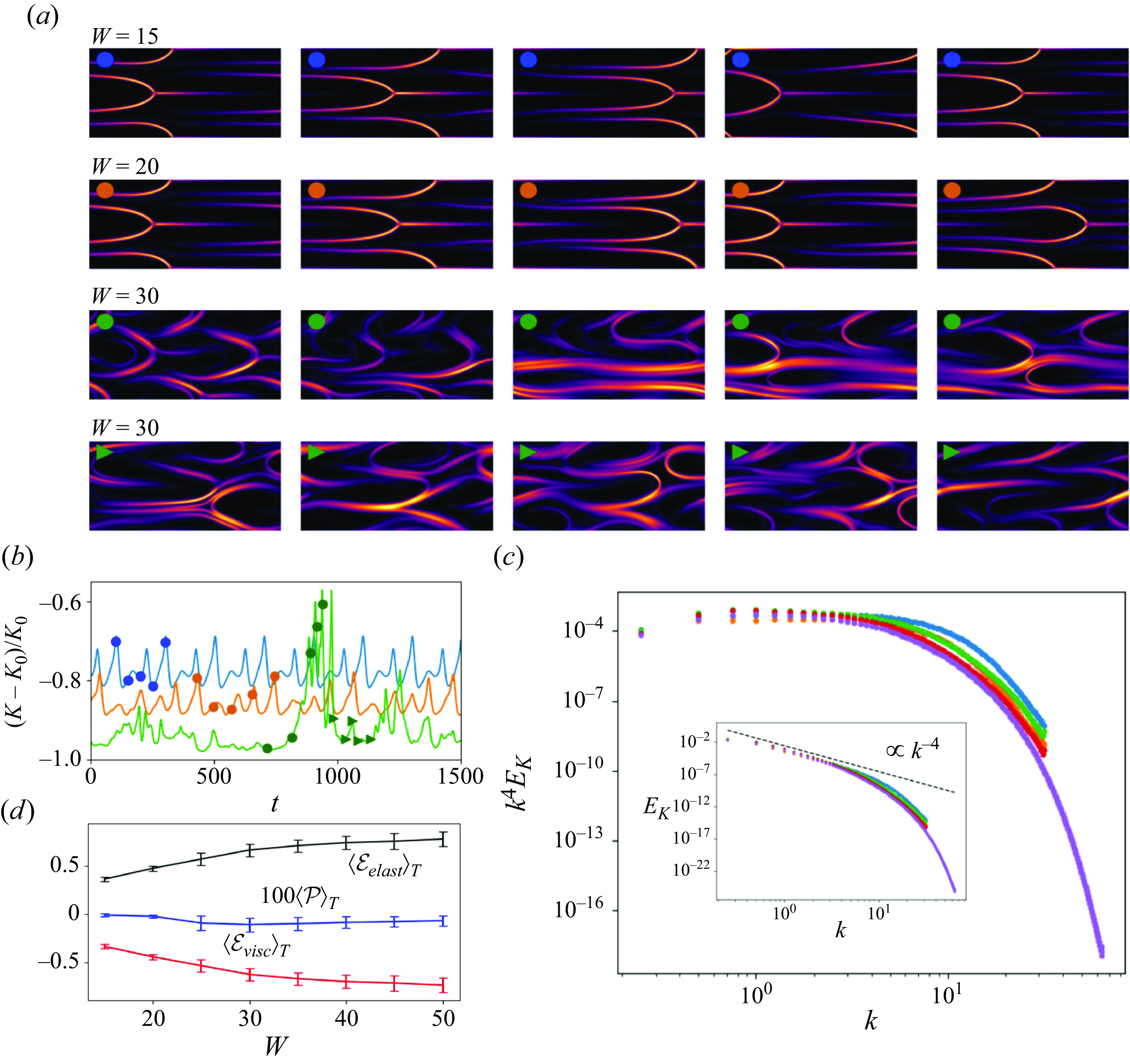
5.2. Elastic turbulence properties
An analysis of ET in vKf is now presented in light of the fact that it occurs due to the centre-mode arrowhead losing stability as $W$
increases. We consider the power spectrum, as well as how energy is produced and dissipated in ET in a domain of
$W$
increases. We consider the power spectrum, as well as how energy is produced and dissipated in ET in a domain of $L_x=8\pi$
where turbulence exists across a wider range of
$L_x=8\pi$
where turbulence exists across a wider range of $W$
(as per figure 13). These are compared with those of the centre-mode arrowhead structure. Three final states are considered: a periodic state at
$W$
(as per figure 13). These are compared with those of the centre-mode arrowhead structure. Three final states are considered: a periodic state at $W=15$
, a weakly chaotic state at
$W=15$
, a weakly chaotic state at $W=20$
and a strongly chaotic at
$W=20$
and a strongly chaotic at $W=30$
(see figure 16). The polymer stress trace field is plotted at various times in figure 16(a), and the kinetic energy time series
$W=30$
(see figure 16). The polymer stress trace field is plotted at various times in figure 16(a), and the kinetic energy time series $K$
normalised by the laminar kinetic energy
$K$
normalised by the laminar kinetic energy $K_0$
in figure 16(b). The periodic state at
$K_0$
in figure 16(b). The periodic state at $W=15$
consists of two arrowheads drifting in the same direction (though still moving relative to each other). The low-dimensional chaos at
$W=15$
consists of two arrowheads drifting in the same direction (though still moving relative to each other). The low-dimensional chaos at $W=20$
again has two arrowheads drifting in the same direction, never making contact with each other. However, the increase in
$W=20$
again has two arrowheads drifting in the same direction, never making contact with each other. However, the increase in $W$
allows the ‘tail’ of the arrowhead to lengthen to the extent it now interacts with its ‘head’. We verify that the dynamics is truly chaotic, rather than quasi-periodic using the classification process discussed in Appendix B. The chaotic state at
$W$
allows the ‘tail’ of the arrowhead to lengthen to the extent it now interacts with its ‘head’. We verify that the dynamics is truly chaotic, rather than quasi-periodic using the classification process discussed in Appendix B. The chaotic state at $W=30$
is more complicated, but we note that two processes can be identified, and we show these in the lower two rows of figure 16(a). The third row shows how multiple arrowheads can join together to form a zonal shear that spans the entire streamwise direction. This is a bursting event in which the kinetic energy peaks. The zonal shear then collapses, splitting into multiple arrowheads. The fourth row shows how the collision, coalescence and subsequent splitting of arrowheads contribute to the turbulent flow.
$W=30$
is more complicated, but we note that two processes can be identified, and we show these in the lower two rows of figure 16(a). The third row shows how multiple arrowheads can join together to form a zonal shear that spans the entire streamwise direction. This is a bursting event in which the kinetic energy peaks. The zonal shear then collapses, splitting into multiple arrowheads. The fourth row shows how the collision, coalescence and subsequent splitting of arrowheads contribute to the turbulent flow.
In figure 16(c) the compensated power spectrum of ET in vKf is plotted for various $W$
which is consistent with
$W$
which is consistent with $E_K\sim k^{-4}$
. This is the scaling found by Foggi Rota et al. (Reference Foggi Rota, Amor, Le Clainche and Rosti2024), Lellep et al. (Reference Lellep, Linkmann and Morozov2024) and Singh et al. (Reference Singh, Perlekar, Mitra and Rosti2024), and is close to that of Berti & Boffetta (Reference Berti and Boffetta2010) who found
$E_K\sim k^{-4}$
. This is the scaling found by Foggi Rota et al. (Reference Foggi Rota, Amor, Le Clainche and Rosti2024), Lellep et al. (Reference Lellep, Linkmann and Morozov2024) and Singh et al. (Reference Singh, Perlekar, Mitra and Rosti2024), and is close to that of Berti & Boffetta (Reference Berti and Boffetta2010) who found $E_K\sim k^{-3.8}$
. Interestingly the periodic state at
$E_K\sim k^{-3.8}$
. Interestingly the periodic state at $W=15$
, the weakly chaotic state at
$W=15$
, the weakly chaotic state at $W=20$
and the strongly chaotic states at
$W=20$
and the strongly chaotic states at $W=30$
all show similar scaling laws, suggesting that the centre-mode arrowhead contains the same small-scale structures present in ET. The region in which this scaling is valid appears to be dependent on
$W=30$
all show similar scaling laws, suggesting that the centre-mode arrowhead contains the same small-scale structures present in ET. The region in which this scaling is valid appears to be dependent on $W$
, with the extent of this region falling with
$W$
, with the extent of this region falling with $W$
. Each of the simulations was run at a resolution of
$W$
. Each of the simulations was run at a resolution of $(N_x, N_y) = (256, 256)$
, except for
$(N_x, N_y) = (256, 256)$
, except for $W=50$
where
$W=50$
where $(N_x, N_y) = (512, 512)$
was used. This high-resolution run gave a power spectrum that was visually similar to that run at the lower resolution (not shown).
$(N_x, N_y) = (512, 512)$
was used. This high-resolution run gave a power spectrum that was visually similar to that run at the lower resolution (not shown).
We now consider the total energy balance and see how the inputted energy due to the base shear compares with the viscous and elastic dissipation. The perturbative kinetic energy budget is derived by expanding the momentum (2.1) about the base state and dotting this with the velocity perturbation $\mathbf {u}^{\prime}$
. This produces
$\mathbf {u}^{\prime}$
. This produces
 \begin{align} Re \left (\frac {\partial u^{\prime}_i}{\partial t} + u^{\prime}_j \partial _j U_i + U_j \partial _j u^{\prime}_i + u^{\prime}_j \partial _j u^{\prime}_i \right ) u^{\prime}_i = \left (- \partial _i p^{\prime} + (1-\beta ) \partial _j \tau ^{\prime}_{ji} + \beta \nabla ^2 u^{\prime}_i \right ) u_i^{\prime} ,\end{align}
where quantities with a prime denote real perturbations from the laminar state, and Einstein summation is used over repeated indices. Incompressibility and the product rule allow us to rewrite this as
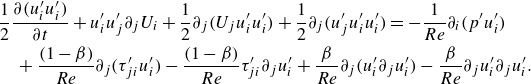 \begin{align} & \frac {1}{2}\frac {\partial (u^{\prime}_i u^{\prime}_i)}{\partial t} + u^{\prime}_i u^{\prime}_j \partial _j U_i + \frac {1}{2} \partial _j ( U_j u^{\prime}_i u^{\prime}_i) + \frac {1}{2} \partial _j (u^{\prime}_j u^{\prime}_i u^{\prime}_i) = - \frac {1}{Re}\partial _i (p^{\prime} u_i^{\prime}) \nonumber\\ & \quad + \frac {(1-\beta )}{Re} \partial _j (\tau ^{\prime}_{ji} u_i^{\prime}) - \frac {(1-\beta )}{Re} \tau ^{\prime}_{ji}\partial _j u_i^{\prime} + \frac {\beta }{Re} \partial _j (u_i^{\prime} \partial _j u^{\prime}_i) - \frac {\beta }{Re} \partial _j u_i^{\prime} \partial _j u^{\prime}_i . \end{align}
Taking a volume average of (5.3) produces an energy budget of
 \begin{align} \frac {\textrm{d}}{\textrm{d}t}(\text{KE}) = \mathcal {P} + \mathcal {E}_{elast} + \mathcal {E}_{visc}, \end{align}
where
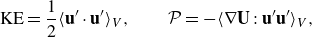 \begin{align} \text{KE} = \frac {1}{2} \langle \mathbf {u^{\prime}} \cdot \mathbf {u^{\prime}} \rangle _V, \qquad \mathcal {P} = -\langle \mathbf {\nabla } \mathbf { U} : \mathbf {u^{\prime}} \mathbf {u^{\prime}} \rangle _V ,\end{align}
 \begin{align} \mathcal {E}_{elast} = -\frac {1-\beta }{Re}\bigl \langle \boldsymbol {\tau ^{\prime}} :{\mathbf {\nabla } \mathbf {u^{\prime}}} \bigr \rangle _V, \qquad \mathcal {E}_{visc} = -\frac {\beta }{Re}\bigl \langle {\nabla \mathbf {u}^{\prime}} : \nabla \mathbf {u^{\prime}} \bigr \rangle _V ,\end{align}
with $\langle \,\cdot \, \rangle _V$
denoting a volume average. This energy budget demonstrates that the kinetic energy can be energised or dissipated via the base shear through
$\langle \,\cdot \, \rangle _V$
denoting a volume average. This energy budget demonstrates that the kinetic energy can be energised or dissipated via the base shear through $\mathcal {P}$
, elastic forces through
$\mathcal {P}$
, elastic forces through $\mathcal {E}_{elast}$
or viscous forces through
$\mathcal {E}_{elast}$
or viscous forces through $\mathcal {E}_{visc}$
. We plot in figure 16(d) the long-time averages of each energising and dissipative term as
$\mathcal {E}_{visc}$
. We plot in figure 16(d) the long-time averages of each energising and dissipative term as $W$
varies, noting that integrating (5.4) over a long time
$W$
varies, noting that integrating (5.4) over a long time $T$
gives
$T$
gives $\langle \mathcal {P}\rangle _T + \langle \mathcal {E}_{elast}\rangle _T + \langle \mathcal {E}_{visc}\rangle _T = 0$
. We see that the only energising process is elasticity, that the base shear contributes little to the kinetic energy and that viscous forces dissipate energy. This is consistent with Buza et al. (Reference Buza, Page and Kerswell2022b
), which considers the energy budget in channel flow of the centre-mode eigenfunctions at higher
$\langle \mathcal {P}\rangle _T + \langle \mathcal {E}_{elast}\rangle _T + \langle \mathcal {E}_{visc}\rangle _T = 0$
. We see that the only energising process is elasticity, that the base shear contributes little to the kinetic energy and that viscous forces dissipate energy. This is consistent with Buza et al. (Reference Buza, Page and Kerswell2022b
), which considers the energy budget in channel flow of the centre-mode eigenfunctions at higher $Re$
. We see that the energy budget is qualitatively similar for flows which are chaotic (
$Re$
. We see that the energy budget is qualitatively similar for flows which are chaotic ( $W=30$
) and for those which are periodic (
$W=30$
) and for those which are periodic ( $W=15$
), but that as
$W=15$
), but that as $W$
increases, elasticity provides more energy to the flow which is dissipated via viscosity.
$W$
increases, elasticity provides more energy to the flow which is dissipated via viscosity.
6. Discussion
In this paper we have found that the only instability operative in 2-D Kolmogorov flow of an Oldroyd-B fluid at vanishing Reynolds number is the centre-mode instability (e.g. PDI does not occur here). As a result, we can confirm that the instability found by Boffetta et al. (Reference Boffetta, Celani, Mazzino, Puliafito and Vergassola2005) at very low $Re$
in Kolmogorov flow is the same instability found at much larger
$Re$
in Kolmogorov flow is the same instability found at much larger $Re$
and
$Re$
and $W$
in pipe flow over a decade later (Garg et al. Reference Garg, Chaudhary, Khalid, Shankar and Subramanian2018). The fact that this instability only exists for
$W$
in pipe flow over a decade later (Garg et al. Reference Garg, Chaudhary, Khalid, Shankar and Subramanian2018). The fact that this instability only exists for $Re \gtrsim 63$
in the pipe flow of an Oldroyd-B fluid (Chaudhary et al. Reference Chaudhary, Garg, Subramanian and Shankar2021) suggested that it was an elasto-inertial instability. It was later shown to be purely elastic in origin, however, by tracking the instability down to
$Re \gtrsim 63$
in the pipe flow of an Oldroyd-B fluid (Chaudhary et al. Reference Chaudhary, Garg, Subramanian and Shankar2021) suggested that it was an elasto-inertial instability. It was later shown to be purely elastic in origin, however, by tracking the instability down to $Re=0$
in channel flow (using the extreme parameter values
$Re=0$
in channel flow (using the extreme parameter values $\beta \gt 0.9905$
and
$\beta \gt 0.9905$
and $W \gt 974$
; Khalid et al. (Reference Khalid, Shankar and Subramanian2021b
)), and by considering the energy budget (Buza et al. Reference Buza, Page and Kerswell2022b
). We have now formally connected the centre-mode instability of the channel and pipe to inertialess Kolmogorov flow, tying together the different flow geometries. The absence of boundaries in Kolmogorov flow is undoubtedly responsible for the substantial downward shift in parameter values, as well as allowing the centre-mode instability to exist at all concentrations
$W \gt 974$
; Khalid et al. (Reference Khalid, Shankar and Subramanian2021b
)), and by considering the energy budget (Buza et al. Reference Buza, Page and Kerswell2022b
). We have now formally connected the centre-mode instability of the channel and pipe to inertialess Kolmogorov flow, tying together the different flow geometries. The absence of boundaries in Kolmogorov flow is undoubtedly responsible for the substantial downward shift in parameter values, as well as allowing the centre-mode instability to exist at all concentrations $\beta \in [0,1)$
and with different wavelengths to the forcing. Floquet analysis reveals that the subharmonic instability (where the instability has a wavelength twice that of the forcing) is usually the most unstable.
$\beta \in [0,1)$
and with different wavelengths to the forcing. Floquet analysis reveals that the subharmonic instability (where the instability has a wavelength twice that of the forcing) is usually the most unstable.
Numerical computations confirm that the centre-mode instability is subcritical with respect to $W$
, as it is in channel flow (Page et al. Reference Page, Dubief and Kerswell2020; Buza et al. Reference Buza, Beneitez, Page and Kerswell2022a
) and pipe flow (Wan et al. Reference Wan, Sun and Zhang2021). The complexity of the nonlinear solutions found increases with the domain length
$W$
, as it is in channel flow (Page et al. Reference Page, Dubief and Kerswell2020; Buza et al. Reference Buza, Beneitez, Page and Kerswell2022a
) and pipe flow (Wan et al. Reference Wan, Sun and Zhang2021). The complexity of the nonlinear solutions found increases with the domain length $L_x$
, the number of forcing wavelengths
$L_x$
, the number of forcing wavelengths $n$
and
$n$
and $W$
but all are built upon arrowhead structures as found earlier by Berti et al. (Reference Berti, Bistagnino, Boffetta, Celani and Musacchio2008) and Berti & Boffetta (Reference Berti and Boffetta2010). Chaotic behaviour occurs only when the domain is long enough (
$W$
but all are built upon arrowhead structures as found earlier by Berti et al. (Reference Berti, Bistagnino, Boffetta, Celani and Musacchio2008) and Berti & Boffetta (Reference Berti and Boffetta2010). Chaotic behaviour occurs only when the domain is long enough ( $L_x$
large enough) with the transition scenario depending on how many forcing wavelengths fit into the domain (i.e.
$L_x$
large enough) with the transition scenario depending on how many forcing wavelengths fit into the domain (i.e. $n$
). Using a domain which allows two forcing wavelengths (
$n$
). Using a domain which allows two forcing wavelengths ( $n=2$
), we identified an irregular bursting scenario after the centre-mode arrowhead structure becomes unstable while a concurrent study finds a period-doubling cascade just including one forcing wavelength (
$n=2$
), we identified an irregular bursting scenario after the centre-mode arrowhead structure becomes unstable while a concurrent study finds a period-doubling cascade just including one forcing wavelength ( $n=1$
) (Nichols et al. Reference Nichols, Guy and Thomases2024). In
$n=1$
) (Nichols et al. Reference Nichols, Guy and Thomases2024). In $n\gt 1$
, the final chaotic or ET state consists of centre-mode arrowheads colliding, coalescing and then splitting up, with a zonal shear forming during bursting events. Power spectra of this chaos show a part of the kinetic energy having a
$n\gt 1$
, the final chaotic or ET state consists of centre-mode arrowheads colliding, coalescing and then splitting up, with a zonal shear forming during bursting events. Power spectra of this chaos show a part of the kinetic energy having a $k^{-4}$
spectrum which is already possessed by the centre-mode arrowhead structure.
$k^{-4}$
spectrum which is already possessed by the centre-mode arrowhead structure.
The sequential ‘supercritical’ transition scenarios seen here and in Nichols et al. (Reference Nichols, Guy and Thomases2024) for 2-D Kolmogorov flow contrast with current observations in channel flow. There, in two dimensions, the arrowheads are stable and so do not sequentially break down to ET (Lellep, Linkmann & Morozov Reference Lellep, Linkmann and Morozov2023) or indeed elasto-inertial turbulence at higher $Re$
(Beneitez et al. Reference Beneitez, Page, Dubief and Kerswell2024a
). In three dimensions, however, there are instabilities which seem to lead to a weak chaotic state (Lellep et al. Reference Lellep, Linkmann and Morozov2023, Reference Lellep, Linkmann and Morozov2024). Presumably the weak chaos seen in three-dimensional channel flow would also be similar to the chaos in three-dimensional Kolmogorov flow which can be explored with far greater ease given the triply periodic boundary conditions. In turn, investigating why 2-D ET can occur in Kolmogorov flow and not obviously in channel flow presents another interesting challenge. In other words, the establishment of a firm instability connection between boundaried and unboundaried viscoelastic straight shear flows can help boost the understanding in either. We hope to report on such progress in the near future.
$Re$
(Beneitez et al. Reference Beneitez, Page, Dubief and Kerswell2024a
). In three dimensions, however, there are instabilities which seem to lead to a weak chaotic state (Lellep et al. Reference Lellep, Linkmann and Morozov2023, Reference Lellep, Linkmann and Morozov2024). Presumably the weak chaos seen in three-dimensional channel flow would also be similar to the chaos in three-dimensional Kolmogorov flow which can be explored with far greater ease given the triply periodic boundary conditions. In turn, investigating why 2-D ET can occur in Kolmogorov flow and not obviously in channel flow presents another interesting challenge. In other words, the establishment of a firm instability connection between boundaried and unboundaried viscoelastic straight shear flows can help boost the understanding in either. We hope to report on such progress in the near future.
Declaration of interests.
The authors report no conflict of interest.
Appendix A. The
$W \rightarrow \infty$
asymptotics for the centre mode in inertialess (
$Re=0$
) Kolmogorov flow


We saw in § 3 that Kolmogorov flow is linearly unstable to the centre mode even when inertia is negligible, and so, motivated by this, we consider the asymptotics when $W \rightarrow \infty$
,
$W \rightarrow \infty$
, $Re=0$
and
$Re=0$
and $\varepsilon =0$
at fixed
$\varepsilon =0$
at fixed $\beta$
. This limit is different to the ‘ultra-dilute’ distinguished limit in which
$\beta$
. This limit is different to the ‘ultra-dilute’ distinguished limit in which $W\rightarrow \infty$
and
$W\rightarrow \infty$
and $\beta \rightarrow 1$
such that
$\beta \rightarrow 1$
such that $W(1-\beta )$
is finite which is required for the centre-mode instability to survive in inertialess channel flow (Khalid et al. Reference Khalid, Shankar and Subramanian2021b
; Kerswell & Page Reference Kerswell and Page2024).
$W(1-\beta )$
is finite which is required for the centre-mode instability to survive in inertialess channel flow (Khalid et al. Reference Khalid, Shankar and Subramanian2021b
; Kerswell & Page Reference Kerswell and Page2024).
Time series of $K$
(left) and frequency spectra
$K$
(left) and frequency spectra $S_K$
(right) at
$S_K$
(right) at $W=80$
(periodic orbit),
$W=80$
(periodic orbit), $W=60$
(quasi-periodic orbit),
$W=60$
(quasi-periodic orbit), $W=20$
(chaos). Other parameters are
$W=20$
(chaos). Other parameters are $Re=0.5$
,
$Re=0.5$
, $\beta =0.95$
,
$\beta =0.95$
, $\varepsilon =10^{-3}$
,
$\varepsilon =10^{-3}$
, $n=2$
and
$n=2$
and $L_x=6\pi$
. These plots correspond to three final states shown in figure 13(b) and demonstrate how the frequency spectra can be used to identify a state as a periodic orbit, quasi-periodic orbit or chaotic.
$L_x=6\pi$
. These plots correspond to three final states shown in figure 13(b) and demonstrate how the frequency spectra can be used to identify a state as a periodic orbit, quasi-periodic orbit or chaotic.

Kinetic energy time series of solutions (left), with the trace field at $t=5000$
(right) as
$t=5000$
(right) as $W$
is lowered from
$W$
is lowered from $W=30$
. The trace field colours use the same scale as figure 14 for comparison purposes. Parameters are
$W=30$
. The trace field colours use the same scale as figure 14 for comparison purposes. Parameters are $\beta =0.95$
,
$\beta =0.95$
, $Re=0.5$
,
$Re=0.5$
, $\varepsilon =10^{-4}$
,
$\varepsilon =10^{-4}$
, $n=2$
and
$n=2$
and $L_x=6\pi$
. Symbols, as in figure 13(a), show chaos (purple star), quasi-periodic orbit (black triangle), periodic orbit (yellow cross) and a travelling wave (green square). This shows that the bursting scenario connecting ET to the centre-mode arrowhead that is seen when
$L_x=6\pi$
. Symbols, as in figure 13(a), show chaos (purple star), quasi-periodic orbit (black triangle), periodic orbit (yellow cross) and a travelling wave (green square). This shows that the bursting scenario connecting ET to the centre-mode arrowhead that is seen when $\varepsilon =10^{-3}$
also exists when
$\varepsilon =10^{-3}$
also exists when $\varepsilon =10^{-4}$
.
$\varepsilon =10^{-4}$
.

The compensated power spectra (regular spectra shown in the inset) when $W=7$
(blue),
$W=7$
(blue), $20$
(orange),
$20$
(orange), $22$
(green),
$22$
(green), $30$
(red) and
$30$
(red) and $\beta =0.95$
,
$\beta =0.95$
, $Re=0.5$
,
$Re=0.5$
, $\varepsilon =10^{-4}$
,
$\varepsilon =10^{-4}$
, $n=2$
and
$n=2$
and $L_x=6\pi$
. This is averaged over a long time (
$L_x=6\pi$
. This is averaged over a long time ( $T=20\,000$
) and shows that
$T=20\,000$
) and shows that $E_K\sim k^{-4}$
.
$E_K\sim k^{-4}$
.
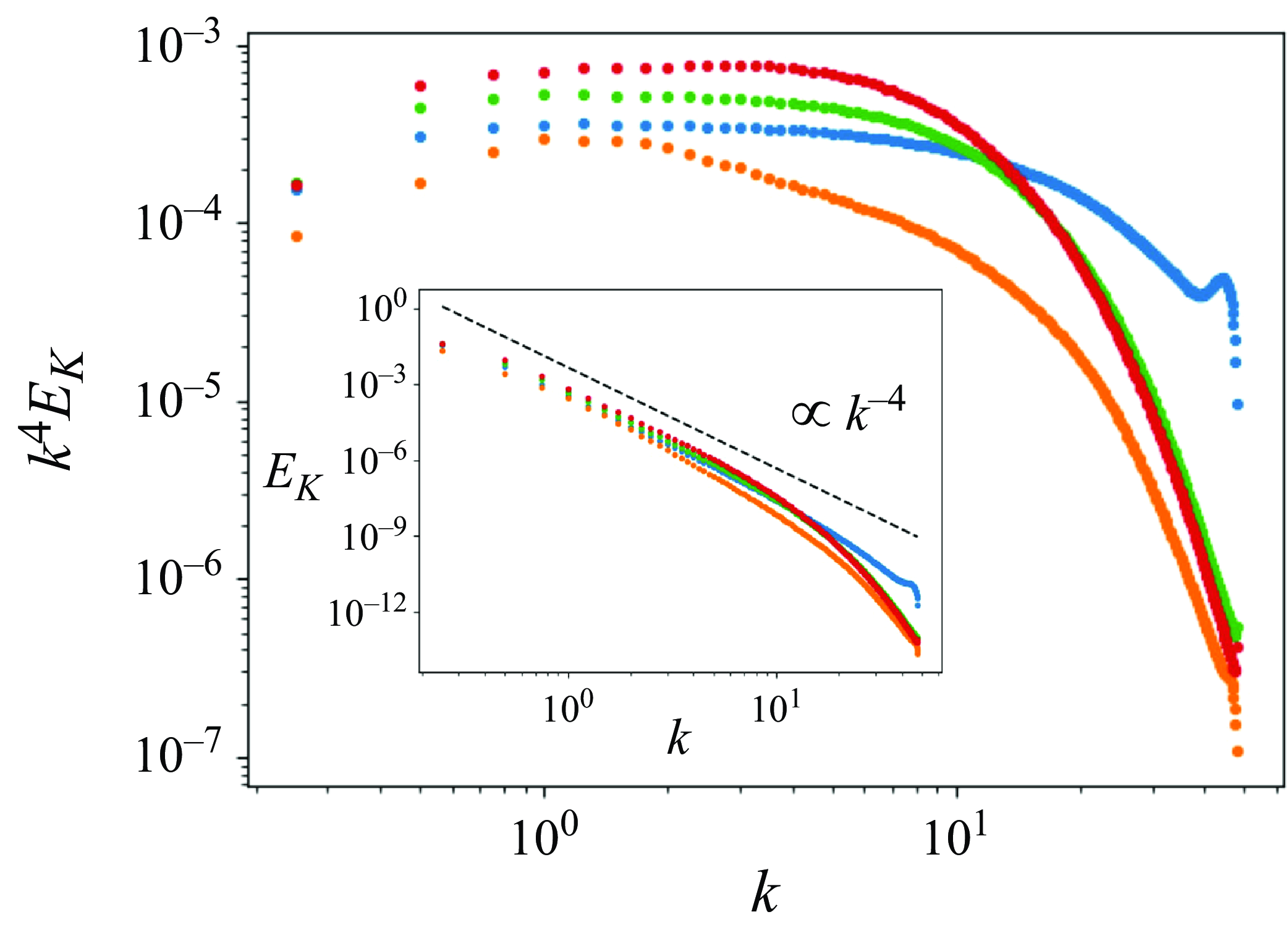
To motivate our scalings we re-examine the collapse of the neutral curves in the $(Re, k)$
plane when
$(Re, k)$
plane when $W\gg 1$
and
$W\gg 1$
and $Re\ll 1$
. This is seen in the
$Re\ll 1$
. This is seen in the $E \gg 1$
main loop of neutral curves of figure 3(d), in regions where
$E \gg 1$
main loop of neutral curves of figure 3(d), in regions where $ERe \gg 1$
. Defining
$ERe \gg 1$
. Defining $k_{max}$
to be the largest wavenumber that is unstable for a set
$k_{max}$
to be the largest wavenumber that is unstable for a set $W$
and
$W$
and $Re$
in this region, we have
$Re$
in this region, we have $k_{max} \sim W^{-1}$
. Motivated by these long-wavelength instabilities, we seek rescalings of
$k_{max} \sim W^{-1}$
. Motivated by these long-wavelength instabilities, we seek rescalings of
 \begin{align} (k, c, u^{\prime}, v^{\prime}, \tau _{xx}^{\prime}, \tau _{xy}^{\prime}, \tau _{yy}^{\prime}, D) = \left(\frac {\hat k}{W}, \hat c, \hat u, \frac {\hat v}{W}, W\hat \tau _{xx}, \hat \tau _{xy}, \frac {\hat \tau _{yy}}{W}, \hat D \right). \end{align}
These factors are determined via considering a dominant balance between the $D\tau _{xx}^{\prime}$
,
$D\tau _{xx}^{\prime}$
, $D^2 \tau _{xy}^{\prime}$
and
$D^2 \tau _{xy}^{\prime}$
and $D^4v^{\prime}$
terms in (2.14), all terms except the last in (2.15) and (2.16) and all the terms in (2.17) and (2.18). In addition, we define
$D^4v^{\prime}$
terms in (2.14), all terms except the last in (2.15) and (2.16) and all the terms in (2.17) and (2.18). In addition, we define
 \begin{align} (U, T_{xx}, T_{xy}) = ( \hat U, W \hat T_{xx}, \hat T_{xy}) \end{align}
so that all base quantities are independent of $W$
. In the limit of
$W$
. In the limit of $W \rightarrow \infty$
, the reduced set of leading-order linearised equations then become
$W \rightarrow \infty$
, the reduced set of leading-order linearised equations then become
 \begin{align} \beta \hat D^4 \hat v = (1-\beta )\left [ -\hat k^2\hat D \hat \tau _{xx} + i\hat k \hat D^2 \hat \tau _{xy} \right ] , \end{align}
 \begin{align} \left [i\hat k(\hat U-\hat c) + 1 \right ]\hat \tau _{xx} = -\hat v \hat D \hat T_{xx} + 2i\hat k \hat T_{xx} \hat u + 2\hat T_{xy} \hat D \hat u + 2\hat \tau _{xy}\hat D\hat U , \end{align}
 \begin{align} \left [i\hat k( \hat U- \hat c) + 1\right ]\hat \tau _{xy} = -\hat v \hat D \hat T_{xy} + i\hat k \hat T_{xx} \hat v + \hat \tau _{yy}\hat D \hat U + \hat D \hat u , \end{align}
 \begin{align} \left [i\hat k( \hat U- \hat c) + 1 \right ] \hat \tau _{yy} = 2i\hat k \hat T_{xy} \hat v + 2 \hat D \hat v , \end{align}
 \begin{align} i\hat k \hat u + \hat D \hat v = 0 . \end{align}
These equations are verified in figures 8 and 9, where the asymptotics are valid as $W\rightarrow \infty$
across a range of
$W\rightarrow \infty$
across a range of $\beta$
and
$\beta$
and $\mu$
. In particular, they are valid even in the UCM limit when
$\mu$
. In particular, they are valid even in the UCM limit when $\beta =0$
(see figure 8
d).
$\beta =0$
(see figure 8
d).
Appendix B. Classification of final states
To classify a final state as laminar, a travelling wave, a periodic orbit, a quasi-periodic orbit or chaotic, we consider the average kinetic energy time series, normalised with respect to the laminar base flow. Our classification protocol is as follows. If $(K-K_0)/K_0$
vanishes, then the state is laminar, while if it tends to a non-zero constant, then the state is a travelling wave. Note that this criterion does not discount equilibria, but in all cases we checked whether the identified solution was stationary on simulating to rule this out. For all fluctuating
$(K-K_0)/K_0$
vanishes, then the state is laminar, while if it tends to a non-zero constant, then the state is a travelling wave. Note that this criterion does not discount equilibria, but in all cases we checked whether the identified solution was stationary on simulating to rule this out. For all fluctuating $(K-K_0)/K_0$
we looked at the frequency spectra by considering the Fourier transform,
$(K-K_0)/K_0$
we looked at the frequency spectra by considering the Fourier transform, $S_K(\omega )$
defined in (5.1), of the time series. Both periodic orbits and quasi-periodic orbits have a discrete number of frequencies with non-zero
$S_K(\omega )$
defined in (5.1), of the time series. Both periodic orbits and quasi-periodic orbits have a discrete number of frequencies with non-zero $S_K(\omega )$
, with the latter having incommensurate frequencies. We characterise a state as chaotic if the frequency spectrum does not consist of discrete frequencies. See figure 17 for an example of periodic, quasi-periodic and chaotic solutions.
$S_K(\omega )$
, with the latter having incommensurate frequencies. We characterise a state as chaotic if the frequency spectrum does not consist of discrete frequencies. See figure 17 for an example of periodic, quasi-periodic and chaotic solutions.
Appendix C. Bursting scenario and power spectra with
$\varepsilon =10^{-4}$

Section 5.1 discusses a bursting scenario leading to ET as $W$
is varied when the polymer stress diffusion coefficient is
$W$
is varied when the polymer stress diffusion coefficient is $\varepsilon =10^{-3}$
. Here, we check that the same results can be qualitatively seen when
$\varepsilon =10^{-3}$
. Here, we check that the same results can be qualitatively seen when $\varepsilon =10^{-4}$
. An increased resolution of
$\varepsilon =10^{-4}$
. An increased resolution of $(N_x, N_y)=(384, 384)$
is used, as decreased diffusion can promote smaller-scale structures, and we verify that final states are sustained when this resolution is increased to
$(N_x, N_y)=(384, 384)$
is used, as decreased diffusion can promote smaller-scale structures, and we verify that final states are sustained when this resolution is increased to $(N_x, N_y)=(512, 512)$
. The behaviour seen when
$(N_x, N_y)=(512, 512)$
. The behaviour seen when $\varepsilon =10^{-3}$
(see figure 14) is also seen with the reduced
$\varepsilon =10^{-3}$
(see figure 14) is also seen with the reduced $\varepsilon =10^{-4}$
in figure 18, at slightly altered
$\varepsilon =10^{-4}$
in figure 18, at slightly altered $W$
. As a fully chaotic state at
$W$
. As a fully chaotic state at $W=30$
is tracked adiabatically down in
$W=30$
is tracked adiabatically down in $W$
, bursting is seen (
$W$
, bursting is seen ( $W=20.7$
), and then the state alternates between periodic orbits (e.g.
$W=20.7$
), and then the state alternates between periodic orbits (e.g. $W=20$
) and quasi-periodic orbits (e.g.
$W=20$
) and quasi-periodic orbits (e.g. $W=14$
) before reaching a travelling wave (
$W=14$
) before reaching a travelling wave ( $W=7$
). In all cases the arrowheads are thinner than when
$W=7$
). In all cases the arrowheads are thinner than when $\varepsilon =10^{-3}$
.
$\varepsilon =10^{-3}$
.
In addition to this we compute the compensated power spectra in figure 19 of the states when $W=7, 20, 22, 30$
, to identify how the power spectra are affected by the reduced
$W=7, 20, 22, 30$
, to identify how the power spectra are affected by the reduced $\varepsilon =10^{-4}$
. These states show a travelling wave (
$\varepsilon =10^{-4}$
. These states show a travelling wave ( $W=7$
), a periodic orbit (
$W=7$
), a periodic orbit ( $W=20$
) and chaos (
$W=20$
) and chaos ( $W=22, 30$
). As seen at larger
$W=22, 30$
). As seen at larger $\varepsilon =10^{-3}$
in figure 16(c), we still find the kinetic energy density generally scales like
$\varepsilon =10^{-3}$
in figure 16(c), we still find the kinetic energy density generally scales like $E_K\sim k^{-4}$
. While this is clear for
$E_K\sim k^{-4}$
. While this is clear for $W=7,\ 22$
and
$W=7,\ 22$
and $30$
, the spectrum of the periodic orbit at
$30$
, the spectrum of the periodic orbit at $W=20$
does not obviously follow this scale. We observed when
$W=20$
does not obviously follow this scale. We observed when $\varepsilon =10^{-3}$
that the extent of the region in which
$\varepsilon =10^{-3}$
that the extent of the region in which $E_K\sim k^{-4}$
decreased with
$E_K\sim k^{-4}$
decreased with $W$
. This appears to be similar here, with the
$W$
. This appears to be similar here, with the $W=7$
compensated spectra being flatter over a larger range of
$W=7$
compensated spectra being flatter over a larger range of $k$
then when
$k$
then when $W=22,30$
. The ranges when
$W=22,30$
. The ranges when $W=22$
and
$W=22$
and $30$
appear reasonably similar, however.
$30$
appear reasonably similar, however.


 Open access