




Introduction
Livestock farming systems (LFSs) must address unprecedented challenges related to food security, sustainability, and societal acceptance. They must meet the demand for protein from a global population projected to reach nearly 10 billion by 2050 (World Bank, 2019), as well as decrease their negative environmental impacts, such as greenhouse gas (GHG) emissions. They must also decrease their consumption of resources, such as water and non-renewable energy (Steinfeld et al., Reference Steinfeld, Gerber, Wassenaar, Castel, Rosales and de Haan2006). Another challenge involves decreasing their impacts on the land used to grow feed in order to preserve ecosystems and their services (Bengtsson et al., Reference Bengtsson, Bullock, Egoh, Everson, Everson, O’Connor, O’Farrell, Smith and Lindborg2019). Farmers must address these challenges while also mitigating the effects of climate change (Allart et al., Reference Allart, Joly, Oostvogels, Mosnier, Gross, Ripoll-Bosch and Dumont2024).
Multiple conceptual and methodological frameworks are available to assess the progress of LFS in addressing these issues. Life cycle assessment, which estimates impacts of products or impacts of the systems that produce them, beginning from the extraction of raw materials (Huppes and Curran, Reference Huppes, Curran and Curran2012), has been increasingly used to assess the climate change impact and other negative impacts, such as eutrophication of water bodies and consumption of fossil fuels (McClelland et al., Reference McClelland, Arndt, Gordon and Thoma2018). Ecosystem services (ES), which are benefits that humans obtain from ecosystems and their processes (Costanza et al., Reference Costanza, d’Arge, de Groot, Farber, Grasso, Hannon, Limburg, Naeem, O’Neil, Paruelo, Raskin, Sutton and van den Belt1997, Reference Costanza, de Groot, Braat, Kubiszewski, Fioramonti, Sutton, Farber and Grasso2017), are used to describe positive contributions of extensive ruminant LFS to human well-being, via grassland ES, such as water purification, erosion prevention, and carbon sequestration (Burkhard et al., Reference Burkhard, Kroll, Nedkov and Müller2012). Agroecology is also used to describe how ES can replace synthetic external inputs with natural processes (Dumont et al., Reference Dumont, Fortun-Lamothe, Jouven, Thomas and Tichit2013). It can occur through replacing veterinary chemicals with bioactive plants, such as chicory, in animal diets (Malsa et al., Reference Malsa, Boudesocque-Delaye, Wimel, Auclair-Ronzaud, Dumont, Mach, Reigner, Guégnard, Chereau, Serreau, Théry-Koné, Sallé and Fleurance2024), or decreasing parasite populations, through parasite dilution, using multi-species livestock grazing (Mugnier, Husson, and Cournut, Reference Mugnier, Husson and Cournut2021; Joly et al., Reference Joly, Note, Barbet, Jacquiet, Faure, Benoit and Dumont2022).
Thus, a variety of frameworks and methods are able to describe and assess positive and negative environmental contributions of LFS to society. These methods, used alone or in combination, can also help describe these contributions as trade-offs, to show that different types of positive contributions may be antagonistic. For example, a provisioning ES, such forage quality, can be high when a regulating ES, such as habitat quality for pollinators, is low, and vice-versa (Klaus et al., Reference Klaus, Richter, Buchmann, Hartmann, Lüscher and Huguenin-Elie2024). The methods can also compare how negative contributions, such as GHG emissions, correlate with biodiversity (Mondière et al., Reference Mondière, Corson, Auberger, Durant, Foray, Glinec, Green, Novak, Signoret and Van Der Werf2024) or regulating ES (Joly et al., Reference Joly, Roche, Fossey, Rebeaud, Dewulf, Van Der Werf and Boone2024). Agroecology can finally describe and assess positive contributions to LFS, while the concept of ecosystem disservices (EDS) can describe negative contributions (Zhang et al., Reference Zhang, Ricketts, Kremen, Carney and Swinton2007), such as pest outbreaks and competition for water or nutrients.
Frameworks that include both negative and positive contributions to LFS have only recently started to receive attention (Oostvogels et al., Reference Oostvogels, Ripoll-Bosch, Allart, Etienne, Nijland, De Boer and Dumont2025). However, the frameworks lack conceptual clarity and objective assessment methods (Saunders, Reference Saunders2020). Furthermore, the ES framework is mostly used to assess the potential supply of services, that is, the level of service that could be provided by an ecosystem, rather than the actual flow of service, representing the benefit delivered by ecosystem (Wang et al., Reference Wang, Zheng, Chen, Ouyang and Hu2022). For example, an ecosystem can potentially provide a high supply of pollination ES if it has large populations of pollinating insects, but the flow of ES is effective only if the insects pollinate a nearby crop or orchard.
Here, we used a graphical tool called the Barn (Dumont et al., Reference Dumont, Ryschawy, Duru, Benoit, Chatellier, Delaby, Donnars, Dupraz, Lemauviel-Lavenant, Méda, Vollet and Sabatier2019; Ryschawy et al., Reference Ryschawy, Dumont, Therond, Donnars, Hendrickson, Benoit and Duru2019) to study the multiple trade-offs between positive and negative contributions that flow from and into LFS. The Barn was developed to study the contributions that flow through five interfaces: (i) markets, (ii) work and employment, (iii) inputs (from off-farm areas), (iv) the environment and climate, and (v) social and cultural factors. We chose this tool for its comprehensiveness and ability to account for positive and negative contributions. Even though some tools and framework exist to assess LFS on environmental, economic, and social dimensions (e.g., Dolman et al., Reference Dolman, Sonneveld, Mollenhorst and De Boer2014; Kokemohr et al., Reference Kokemohr, Escobar, Mertens, Mosnier, Pirlo, Veysset and Kuhn2022; Leite et al., Reference Leite, Faverin, Ciganda, Cristobal-Carballo, Dos Reis, Eugène, Fariña, Hercher-Pasteur, Monteiro, Pastell, Recavarren, Romera, Rosanowski, Tieri, Aubry, Veysset, Kenny and Vibart2024), the barn is, as far as we know, the only operational tools able to integrate EDS. We applied it to lamb meat systems for their importance in terms of environmental challenges. Sheep farming is widespread, and in 2024, there were 1.4 Md of sheep heads in the world, which is comparable to the number of cattle heads (1.6 Md) (FAO, 2026). Beef and sheep meat have in addition the first and second most important footprint in terms greenhouse gas emissions and land use per kg of protein of all animal protein sources (Poore and Nemecek, Reference Poore and Nemecek2018).
We, therefore, applied the Barn to five lamb meat systems in France and Ireland, where sheep is the second most abundant livestock after cattle, with number of heads of 6.6 and 3.6 M, respectively (FAO, 2026). Each system corresponds to a real farm whose environmental and production performances, such as GHG emissions and ewe productivity, have been studied extensively (Benoit et al., Reference Benoit, Sabatier, Lasseur, Creighton and Dumont2019). Studies have also investigated the adaptation of the systems to meat-sector requirements (Benoit et al., Reference Benoit, Sabatier, Lasseur, Creighton and Dumont2019) and resilience to technical and economic hazards (Benoit et al., Reference Benoit, Joly, Blanc, Dumont, Sabatier and Mosnier2020). By assessing positive and negative contributions (hereafter, ‘services’ and ‘disservices’, respectively), these studies provided the baseline information required to apply the Barn. The objectives of the present study were to (i) identify the services and disservices flowing from and into the LFS, (ii) quantify these services and disservices, and (iii) analyze trade-offs between these services and disservices.
Materials and methods
Livestock farming systems studied
The five LFSs studied (four in France and one in Ireland) are located in several geographic and climate contexts and had contrasting strategies for reproduction and animal feeding (see Benoit et al. (Reference Benoit, Sabatier, Lasseur, Creighton and Dumont2019) for details). ‘Graz’, located in the lowlands of western France, was a grazing system based on a main lambing period at the end of winter. LFS ‘3 × 2’, located in the Massif Central uplands of France, had a specific reproduction strategy, with three lambings every 2 years, and used concentrates to produce lambs indoors. OF (organic farming), also in the Massif Central uplands, was an organic system with two lambing periods. DT (dual transhumant), located in the Mediterranean region of France, was based mainly on year-round grazing of rangelands and other semi-natural land-cover categories, by a hardy sheep breed with low prolificacy. DT’s lambs were not fed concentrates, and its males were sold at 12–18 months of age; some female lambs were also sold at weaning for fattening. ‘Irel’, the LFS in Ireland, was a system with one lambing period per year with grass-fattened lambs in a humid oceanic climate. Among the five LFSs, ewe productivity ranged from 0.82 to 1.66 lambs per ewe >6 months old, and concentrate consumption ranged from 0 to 134.6 kg/ewe/yr (Table 1).
Key characteristics of the five livestock farming systems studied

Table 1. Long description
The table has six rows for characteristics and five columns for farming systems labeled Irel, Graz, 3 × 2, OF, and DT. From left to right, the first row lists number of ewes over 6 months old as 420, 541, 470, 405, and 2,105. The second row shows workers in annual work units as 1.00, 1.50, 1.50, 1.00, and 4.67. The third row gives ewe productivity in lambs per ewe over 6 months old as 1.54, 1.33, 1.66, 1.32, and 0.82. The fourth row presents concentrates fed per kilogram carcass as 1.22, 1.55, 5.24, 3.41, and 0.00. The fifth row shows concentrates fed per ewe per year as 36.5, 42.2, 134.6, 77.1, and 0.0. The sixth row lists feed self-sufficiency percentage as 94.9, 94.3, 78.2, 88.1, and 100.0. A footnote clarifies that feed self-sufficiency is the percentage of the flock’s annual energy needs provided by on-farm feed resources. System abbreviations are defined as Irel for Ireland, Graz for grazing, 3 × 2 for three lambings in two years, OF for organic farming, and DT for dual transhumant.
1 Percentage of the flock’s annual energy needs provided by on-farm feed resources.
Note: Irel = Ireland, Graz = grazing, 3 × 2 = three lambings in 2 years, OF = organic farming, and DT = dual transhumant.
Representation and assessment of services and disservices
Representation of services and disservices
In the Barn, both services and disservices flow into LFS (i.e. inwards toward the Barn) and from LFS (i.e. outwards from the Barn) (Fig. 1). The flow of services and disservices are, respectively, represented by green and red arrows, the width of which represent the magnitude of the service or the disservice. Services and disservices can flow jointly, and in such case, they are represented by a hatched arrow (Fig. 1). It occurs, for example, in the work and employment interface when many jobs are generated, but the jobs have difficult working conditions (e.g., in a slaughterhouse). Outward flows represent services or disservices from LFS to society or other agricultural sectors. Services from LFS to society in the environment and climate interface can be regulating ES, such as pollination, whereas disservices can be GHG emissions. Services into LFS can be ES used for livestock production (hereafter, ‘input ES’), such as the supply of natural forage, whereas disservices to LFS can be carnivore predation.
Services (green) and disservices (red) flowing from and into two lamb meat systems (graz = grazing and 3 × 2 = three lambings in 2 years) according to the Barn graphical tool. Services and disservices can flow jointly in the same time (hatched arrow). The pictograms were defined by Ryschawy et al. (Reference Ryschawy, Dumont, Therond, Donnars, Hendrickson, Benoit and Duru2019).

Figure 1. Long description
The top panel shows a pentagonal diagram labeled Graz, with a central sheep icon surrounded by permanent and temporary grasslands. Green arrows indicate services flowing outward to markets, work and employment, social and cultural factors, and environment and climate. Red arrows indicate disservices, including hatched arrows for joint flows. Inputs are shown at the base with icons for feed and resources. The bottom panel, labeled 3 x 2, has a similar structure but includes additional icons for disservices such as pests and waste, and a factory icon within the pentagon. Both panels use pictograms for each factor, and the legend distinguishes permanent from temporary grasslands.
The Barn has been used mainly to compare livestock production areas (Vollet et al., Reference Vollet, Huguenin-Elie, Martin and Dumont2017; Dumont et al., Reference Dumont, Ryschawy, Duru, Benoit, Chatellier, Delaby, Donnars, Dupraz, Lemauviel-Lavenant, Méda, Vollet and Sabatier2019) or promote discussions among local stakeholders about the opportunities and threats that LFS face (Dernat, Dumont, and Vollet, Reference Dernat, Dumont and Vollet2023). To date, the tool has been applied using a semi-quantitative approach, to represent visually the flow of ES and EDS, with the width of the arrows. Here, we used it to help precisely quantify services and disservices and identify their trade-offs.
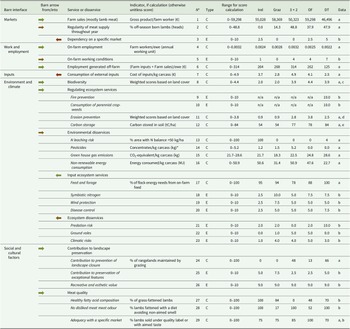
For each of the five Barn interfaces, we calculated service and disservice scores that ranged from 0 (worst) to 10 (best). The scores equaled the mean of one to four sub-scores which were based on indicator values (Table 2). A score of 10 was usually attributed to the highest indicator value among the five LFSs, whereas a score of 0 was attributed either to the lowest indicator value among the LFS or to an indicator value of 0. We used this approach to set the minimum and maximum scores for context-dependence reasons. For example, for the minimum pertinent value, most indicators can have a value of 0 (e.g., use of external inputs), but others cannot (e.g., GHG emissions, because ruminant farming cannot avoid emitting methane). The ranges of minimum and maximum values of each indicator are given in Table 2, and between these values, intermediate sub-scores were linearly interpolated. For the indicators for which a lower value indicated higher performance (e.g., use of external inputs), the interpolated score was subtracted from 10 to invert it. When no quantitative indicator was available for a given service or disservice (12 of 29), its sub-score was based on expert knowledge, as commonly done in ES-related studies (Burkhard et al., Reference Burkhard, Kroll, Nedkov and Müller2012; Stoll et al., Reference Stoll, Frenzel, Burkhard, Adamescu, Augustaitis, Baeßler, Bonet, Carranza, Cazacu, Cosor, Díaz-Delgado, Grandin, Haase, Hämäläinen, Loke, Müller, Stanisci, Staszewski and Müller2015; Campagne and Roche, Reference Campagne and Roche2018). This knowledge was provided by the co-authors themselves, who have expertise in lamb production and economics, life-cycle assessment, ecology and ecosystem services, and agro-ecological transition. For each service or disservice considered, they assigned a sub-score based on the known minimum and maximum levels within the study context.
Indicator values used to assess the scores for services and disservices flowing from and into the five lamb meat systems studied

Table 2. Long description
The table is organized into five main groups: Markets, Work and employment, Inputs, Environment and climate, and Social and cultural factors. Each group is subdivided by barn interface and service or disservice. Columns from left to right are: Barn interface, Barn arrow from or into, Service or disservice, Indicator (if calculation, otherwise unitless score), N superscript o, Type (C for calculation, E for expert knowledge), Range for score calculation, and five columns for lamb meat systems (Irel, Graz, 3 times 2, O F, D T), followed by a Data source column. For Markets, indicators include farm sales (gross product per farm worker, values: Irel 55,028; Graz 58,369; 3 times 2 50,323; O F 59,298; D T 46,496), regularity of meat supply (percent off-season born lambs, Irel 0.0; Graz 14.3; 3 times 2 48.8; O F 37.9; D T 47.9), and dependency on a specific market (score out of 10, Irel 2.5; Graz 0; 3 times 2 0; O F 2.5; D T 5). Work and employment includes on-farm employment (farm workers per ewe, Irel 0.0024; Graz 0.0028; 3 times 2 0.0032; O F 0.0025; D T 0.0022), on-farm working conditions (score out of 10, Irel 1; Graz 0; 3 times 2 4; O F 4; D T 7), and off-farm employment ((farm inputs plus farm sales) per ewe, Irel 264; Graz 268; 3 times 2 314; O F 262; D T 125). Inputs are measured by cost of inputs per kilogram carcass (Irel 3.7; Graz 2.8; 3 times 2 4.9; O F 4.1; D T 2.5). Environment and climate covers biodiversity (weighted scores, Irel 2.0; Graz 2.0; 3 times 2 3.9; O F 4.4; D T 3.9), regulating ecosystem services (sub-indicators: fire prevention, consumption of perennial crop-weeds, erosion prevention, carbon storage), environmental disservices (N leaching risk, pesticides, greenhouse gas emissions, non-renewable energy consumption), input ecosystem services (feed and forage, symbiotic nitrogen, wind protection, disease control), and ecosystem disservices (predation risk, ground voles, climatic risks). Social and cultural factors include contribution to landscape preservation, prevention of landscape closure (percent rangelands maintained by grazing), preservation of exceptional features, recreative and esthetic value, meat quality (healthy fatty acid composition, absence of non-aimed meat odor, adequacy with specific market). Data sources are coded as a, b, c, d, or e, referencing specific studies. The table uses green arrows for services, red for disservices, and hatched arrows for simultaneous flows.
Note: C = calculation, E = expert knowledge; *0 for OF because its 3.41 kg concentrates/kg carcass had not received pesticide applications; n/a = not applicable. Irel = Ireland, Graz = grazing, 3 × 2 = three lambings in 2 years, OF = organic farming, and DT = dual transhumant. The color of the arrows represents a service (green) or disservice (red). Hatched arrows represent services and disservices that flow at the same time from/into systems. Sub-indicators are in italics and were averaged after normalization to calculate the final scores (Table 3).
Data: a = Benoit et al. (Reference Benoit, Sabatier, Lasseur, Creighton and Dumont2019), b = this study, c = Burkhard et al. (Reference Burkhard, Kroll, Nedkov and Müller2012), d = Burkhard et al. (Reference Burkhard, Kandziora, Hou and Müller2014), e = Pellerin et al. (Reference Pellerin, Bamière, Launay and Martin2020).
Quantification of services and disservices by interface
Markets. The markets interface (indicators 1–3) represents the integration of LFS into the livestock sector. Indicators 1 and 2 represented services and disservices flowing from LFS, and indicator 1 assessed production performance as gross product per worker (€). Higher product yielded a higher score. We chose this economic indicator instead of a biophysical indicator such as kg of carcass or number of lambs, to compare LFS located in different climates (oceanic for Irel, Mediterranean for DT, and continental for the other three LFSs), in a more relevant manner. Indicator 2 assessed the distribution of the supply of lamb meat throughout the year, as the percentage of lambs born outside the grazing season. A higher percentage made production more stable and yielded a higher score. Indicator 3 assessed whether LFS depended on a specific market or not; greater dependence yielded a lower score. Indicators 1 and 2 were calculated using data from Benoit et al. (Reference Benoit, Sabatier, Lasseur, Creighton and Dumont2019), whereas indicator 3 was expert-based.
Work and employment. The work and employment interface (indicators 4–6) represents the contribution of LFS to employment through services and disservices, flowing from LFS. Indicator 4 assessed the number of jobs provided on-farm as the number of farm workers per ewe. Larger numbers yielded higher scores, indicating that LFS provided jobs for more people. Indicator 5 assessed the quality of the jobs provided by describing whether they were pleasant or not (e.g., working in a slaughterhouse can be tedious and exposes to injury risks). Indicator 6 assessed the number of jobs provided off-farm as an indicator of upstream and downstream economic activity: the sum of the costs of LFS external inputs plus LFS sales in € per ewe. Indicators 4 and 6 were calculated using data from Benoit et al. (Reference Benoit, Sabatier, Lasseur, Creighton and Dumont2019), whereas indicator 5 was expert-based.
Inputs. The inputs interface (indicator 7) represents the optimal use of local resources to produce lamb meat. Indicator 7 assessed the cost of external inputs in € per kg of carcass, which aggregated inputs expressed in different units, such as kg (concentrates) or MJ (non-renewable energy). Higher costs yielded lower scores. Indicator 7 was calculated using data from Benoit et al. (Reference Benoit, Sabatier, Lasseur, Creighton and Dumont2019).
Environment and climate. The environment and climate interface represents services and disservices flowing from LFS (8–16) and into LFS (17–23). Indicator 8 assessed biodiversity as a function of land-cover scores obtained from the capacity matrix of Burkhard et al. (Reference Burkhard, Kroll, Nedkov and Müller2012). This matrix provides scores of biodiversity and ES for a wide range of land-cover categories (e.g., crops, grasslands, forests). We calculated the mean scores of the LFS for both on-farm and off-farm areas, weighted by the relative areas of land-cover categories. We used the following equivalences between the land-cover categories of Burkhard et al. (Reference Burkhard, Kroll, Nedkov and Müller2012) and those of the present study: ‘Pasture’ for temporary grasslands less than 5 years old, ‘Natural grassland’ for permanent grasslands (i.e. more than 5 years old) in lowlands and all upland grasslands, and ‘Moors and heathland’ for rangelands. To consider the benefits of organic farming for biodiversity (Klaus et al., Reference Klaus, Jehle, Richter, Buchmann, Knop and Lüscher2023; Gerling et al., Reference Gerling, Sturm and Wätzold2019), we adjusted Burkhard’s biodiversity indices using the biodiversity-gain indices developed by Knudsen et al. (Reference Knudsen, Hermansen, Cederberg, Herzog, Vale, Jeanneret, Sarthou, Friedel, Balázs, Fjellstad, Kainz, Wolfrum and Dennis2017). They concerned crop and grassland areas, which were 61.2% and 8.9% higher in organic LFS, respectively, than in conventional LFS. Indicators 9 and 10 represented the level of regulating ES supplied such as erosion prevention and carbon storage, respectively. Erosion prevention was calculated, like biodiversity, using land-cover and capacity-matrix scores (Burkhard et al., Reference Burkhard, Kandziora, Hou and Müller2014). Carbon storage expressed as t of carbon stored in the soil per ha was calculated using the land-cover categories and carbon stock per land-cover category of Pellerin et al. (Reference Pellerin, Bamière, Launay and Martin2020). Indicators 11 and 12 represented the regulating ES of vineyard weeding and wildfire prevention, respectively, which were relevant only for the landscapes around DT. Thus, they were considered only for DT and were expert-based. Indicators 13–16 represented environmental disservices related to pollution and energy consumption. Indicator 13 assessed nitrogen (N) leaching as the percentage (calculated) of an LFS’s area on which the N balance exceeded 50 kg N/ha, based on Van Grinsven et al. (Reference Van Grinsven, Ten Berge, Dalgaard, Fraters, Durand, Hart, Hofman, Jacobsen, Lalor, Lesschen, Osterburg, Richards, Techen, Vertès, Webb and Willems2012). Indicator 14 represented pesticide use through the proxy of the feeding of concentrates, which are produced from crops (set to 0 for OF). It was calculated as kg of concentrates fed per kg of carcass. Indicators 15 and 16 represented GHG emissions (kg CO2-eq. per kg of carcass) and consumption of non-renewable energy (MJ per kg of carcass), respectively. They were estimated using life cycle assessment in the French Dia’Terre tool, which is based on the GES’TIM model (Gac et al., Reference Gac, Cariolle, Deltour, Dollé, Espagnol, Flénet, Guingand, Lagadec, Le Gall, Lellahi, Malaval, Ponchant and Tailleur2011) (see Benoit et al. (Reference Benoit, Sabatier, Lasseur, Creighton and Dumont2019) for details).
For the services and disservices flowing into LFS, indicators 17–20 represented input ES. Indicator 17 represented the provisioning ES of forage, which ensures feed self-sufficiency, and was expressed as the calculated percentage of the flock’s energy requirements provided by on-farm areas. Indicator 18 represented regulating ES related to N fixation by legumes. It was expert-based because no field measurements were available, and it was based on the knowledge of each LFS’s strategy for increasing legume production. For example, on Graz, temporary grasslands were renewed every 5 years using a seed mixture with a high clover content. OF adopted the same practice on temporary grasslands and also kept permanent grasslands short to increase legume abundance, especially in spring, since shading decreases legume growth (Simon, Gastal, and Lemaire, Reference Simon, Gastal and Lemaire1989). Indicator 19 represented wind protection provided by LFS topography and landscape infrastructure, such as hedges, and was expert-based. Indicator 20 represented disease control provided by grassland plants with high tannin concentrations that can mitigate gastro-intestinal parasites (Hoste et al., Reference Hoste, Torres-Acosta, Sandoval-Castro, Mueller-Harvey, Sotiraki, Louvandini, Thamsborg and Terrill2015). It was expert-based, depending on the percentage of natural grasslands and rangelands on the LFS, where such plants are more likely to grow than on temporary grasslands, whose sown species are chosen. Indicators 21–23 represented EDS and were also expert-based. A high score represented a low exposure to EDS. Indicator 21 represented the risk of predation from foxes, stray dogs, or wolves, whereas indicator 22 represented the risk of grassland degradation due to rodent outbreaks (e.g., ground voles). Indicator 23 represented the risk of forage shortage and was based on the local climate and the variety of resources available to buffer droughts.
Social and cultural factors. The social and cultural factors interface represented services from LFS through their contribution to landscape preservation (indicators 24–26) and product quality (indicators 27–29). Indicator 24 represented the contribution to maintaining open landscapes threatened by brush encroachment and/or conifer plantations. It assessed the percentage (calculated) of rangelands on the LFS because they can be used for livestock production only through grazing (unlike temporary grasslands, which can be converted to croplands). Indicator 25 represented the contribution to maintaining exceptional landscape features, such as hedges with centuries-old oaks. Indicator 26 represented the recreational and esthetic value of the landscapes; indicators 25 and 26 were expert-based.
Indicator 27 represented the nutritional quality of meat by reflecting that grazing improves the composition of fatty acids in meat that are beneficial to human health (Aurousseau et al., Reference Aurousseau, Bauchart, Faure, Galot, Prache, Micol and Priolo2007). Indicator 27 assessed the percentage of lambs in the flock that were fattened by grazing outdoors (calculated). Indicator 28 represented the absence of the market risk caused by a strong smell in the meat. Because consuming legumes can cause this strong smell, grazing grasslands increases this risk (Prache, Reference Prache, Bellon and Penvern2014). Thus, indicator 28 assessed the percentage of lambs fattened with either concentrates or grass without legumes (calculated). Higher percentages yielded higher scores, except for DT, which received a score of 10 because its primary market (those celebrating Eid al-Adha) has no problem with, and even appreciates, lamb meat with this smell. Finally, indicator 29 represented the quality of lamb meat as the percentage (calculated) of lambs sold under a specific label of quality or origin, or with a particular ability to meet market demand for its meat (e.g., DT).
Results
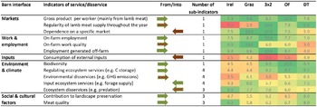
According to the values of the indicators (Table 2), the main services and disservices of the LFS varied, as did their trade-offs (Table 3).
Summary of the scores for services and disservices flowing from and into livestock farming systems

Table 3. Long description
The table is organized with livestock farming systems as rows and types of services or disservices as columns. Each cell contains an arrow indicating the flow direction, with green for services and red for disservices. Hatched arrows show simultaneous service and disservice flows. Systems include abbreviations such as Irel for Ireland, Graz for grazing, 3 times 2 for three lambings in two years, OF for organic farming, and DT for dual transhumant. High scores in service columns indicate high service levels, while high scores in disservice columns indicate low disservice levels. G H G stands for greenhouse gases. The table enables comparison of the magnitude and direction of ecosystem services and disservices across different livestock systems.
Note: Irel = Ireland, Graz = grazing, 3 × 2 = three lambings in 2 years, OF = organic farming, and DT = dual transhumant. The color of the arrows represents a service (green) or disservice (red). Hatched arrows represent services and disservices that flow at the same time from/into systems. For services, a high score represents a high level of service; for disservices, a high score represents a low level of disservice. GHG = greenhouse gases.
Irel system
Irel was productive, as indicated by its high score for gross product per worker, but its dependence on grasslands made it highly seasonal, which explained its low score for meat-supply regularity. The LFS supports a dynamic livestock sector and had only one workload peak per year due to its seasonality, which explained its high scores in the work and employment interface (Table 3). Irel’s feeding system contained only temporary grasslands, often monocultures of perennial ryegrass, that were fertilized with large amounts of synthetic N fertilizers and had a high stocking rate, which explained its low scores in the inputs and environment and climate interfaces. In this type of highly intensively management landscape, only foxes could prey on lambs, which explains its high EDS score (e.g., low exposition to EDS). Irel produced a well-appreciated meat and helped shape the typical green Irish landscape, which explained the high levels of most indicators in the social and cultural factors interface.
Graz system
Graz was also relatively productive and sold products in several French markets, which explained its high score for gross product per worker. It was also seasonal, which decreased its score for meat-supply regularity, which was, however, slightly higher than that of Irel due to having a certain percentage of off-season lambing. Graz used fewer external inputs than Irel did, which explained its higher score for the inputs interface. N-fixing legumes, along with hedges that provided wind protection, resulted in a high score for the input ES flowing into Graz, but the legumes increased the risk of a strong smell in the meat. The hedges and trees also increased the risk of fox predation, and the large amount of grass used for feeding exposed Graz to the risk of forage shortage. Thus, Graz had moderate scores for disservices into LFS in the environment and climate interface. Graz also shaped the popular bocage landscape, consisting of a mosaic of grasslands, hedges, and old oaks, which explained the high level of the indicator of recreational and esthetic value.
3 × 2 system
LFS 3 × 2 was highly productive due to its three lambing periods over 2 years, which is possible because ewes can give birth three times per year. This high productivity was based on feeding large amounts of concentrates and indoors, which gave it the lowest input ES score among the five LFS. LFS 3 × 2 provided a regular supply of meat, which was able to meet peaks in demand during Easter and Christmas. By being able to meet the demand of the meat sector via productivity and consistency, it received high scores overall in the markets interface. This productivity and consistency also generated upstream and downstream employment, which explained its high scores in the work and employment interface, except for work quality, whose score was moderate due to the three lambing periods. Its land use consisted mainly of permanent grasslands, which explained its high biodiversity and regulating ES scores. However, this high percentage of permanent grasslands represented a risk of damage during vole outbreaks, which explained its low score for EDS. However, 3 × 2 could mitigate damage to grasslands and the resulting impacts on livestock production because of its ability to produce lambs three times per year, due to feeding large amounts of concentrates. This practice made it possible to avoid having non-pregnant ewes for long periods and provided a compensatory mechanism of resilience.
OF system
OF was productive because it had two lambing periods per year due to feeding large amounts of concentrates. This high livestock productivity explained the moderate-to-high scores in the markets interface, but the use of such large amounts of concentrates gave it a low disservice score in the inputs interface. The two lambing periods also complicated work, which explained its low score for work quality in the work and employment interface. OF also depended only on the organic market, which decreased its score for market dependence. OF had high percentages of permanent grasslands and rangelands and was organic, which explained its high scores for biodiversity and regulating ES in the environment and climate interface. OF was also sensitive to predation and forage shortage due to summer drought, which explained its low disservice scores in the environment and climate interface.
DT system
DT had low ewe productivity, which generated the least income per worker among the five LFSs. It also had demanding work due to its transhumant nature, which required transporting animals over long distances and protecting flocks from predation. It sold mainly old lambs whose meat had a strong smell, which was suitable only for a specific market. These characteristics explained its low-to-moderate scores in the markets and work and employment interfaces, except for meat-supply regularity due to its potential for off-season lambing (supported by the variety of forages available in the climate of southern France and the low breed prolificacy, which requires less energy). DT used few inputs and was self-sufficient in feed, which gave it the highest score for the inputs interface among the five LFSs. Its transhumant grazing maintained a variety of semi-natural grasslands and rangelands, weeded vineyard rows, and prevented brush encroachment, which contributed to wildfire prevention. This strategy explained its high biodiversity and regulating ES scores in the environment and climate interface. However, predation by foxes and wolves, in addition to the risk of forage shortage due to drought, resulted in the lowest score for EDS among the five LFSs. Finally, the vast alpine areas managed by its grazing helped maintain iconic alpine landscapes, which gave it the highest score for landscape preservation in the social and cultural factors interface, among the five LFSs.
Discussion
Trade-offs between services and disservices flowing from and into livestock farming systems
Unsurprisingly, none of the LFS performed well in all five Barn interfaces for services flowing from LFS, and we observed the usual trade-off between production and the environment. For example, Graz was productive and generated high income per worker, but provided few environmental services, which was the opposite for DT. This trade-off is commonly illustrated by the antagonism between provisioning ES (i.e. livestock production) and regulating ES (i.e. positive environmental contributions) (Maes et al., Reference Maes, Paracchini, Zulian, Dunbar and Alkemade2012; Bekele et al., Reference Bekele, Lant, Soman and Misgna2013; Holt et al., Reference Holt, Alix, Thompson and Maltby2016; Bengtsson et al., Reference Bengtsson, Bullock, Egoh, Everson, Everson, O’Connor, O’Farrell, Smith and Lindborg2019; Mondière et al., Reference Mondière, Corson, Auberger, Durant, Foray, Glinec, Green, Novak, Signoret and Van Der Werf2024; Klaus et al., Reference Klaus, Richter, Buchmann, Hartmann, Lüscher and Huguenin-Elie2024). We also observed how market services from LFS can come with disservices, such as the quality of the job provided. Other studies have also observed this antagonism between livestock production and job quality (Slade and Alleyne, Reference Slade and Alleyne2023) but, to the best of our knowledge, it is not specifically and extensively studied in terms of trade-off involving negative and positive contributions of LFS. We also observed no clear trade-off between social and cultural factors and other services. For example, Irel and OF had similar values of indicators of the contribution to landscape preservation, but Irel had much lower scores for biodiversity and regulating ES than OF did. This pattern was similar to those observed elsewhere, with no straightforward relation between management intensity and the attractiveness of grasslands for recreation across studies (Le Clec’h et al., Reference Le Clec’h, Finger, Buchmann, Gosal, Hörtnagl, Huguenin-Elie, Jeanneret, Lüscher, Schneider and Huber2019; Schmitt et al., Reference Schmitt, Haensel, Kaim, Lee, Reinermann and Koellner2024). It could be explained by the fact the main benefits of grasslands are the open views they provide (Chai-allah et al., Reference Chai-allah, Hermes, La Foye, Venter, Joly, Brunschwig, Bimonte and Fox2025), which indicates that their simple presence supplies cultural ES, regardless of their nature or management. It could also be because LFSs have shaped their landscapes over centuries and are thus accepted as such. However, it is difficult to further interpret these patterns because the attractiveness and recreation potential of landscapes are subjective (Khaledi, Khakzand, and Faizi, Reference Khaledi, Khakzand and Faizi2022) and depend on social categories (Tveit, Reference Tveit2009). We thus used the Barn to describe a variety of trade-offs between different types of services flowing from LFS, with differing degrees of trade-offs. Some of these trade-offs are well known and studied, such as that between production and the environment, but others that involve work quality and cultural contributions may require further study.
We also observed trade-offs between certain services and disservices flowing from and into LFS. Irel and Graz, based on temporary grasslands, had high scores in the markets interface but low scores in the environment and climate interface (services flowing from LFS). Irel and Graz consumed large and moderate amounts of external inputs, respectively, but Graz supplemented its external inputs with a high level of input ES, especially nitrogen fixation. This indicates that, to a certain extent, external inputs and input ES can replace each other. However, Graz’s high level of input ES for production exposed it to EDS, which indicates that strong dependence on input ES for livestock production comes with EDS. Three LFSs (3 × 2, OF, and DT) had a high percentage of permanent grasslands and relatively high scores for services from LFS in the environment and climate interface, but lower scores for EDS into LFS. Despite these low EDS scores, 3 × 2 maintained high scores for services from LFS in the markets interface, because its three lambing periods resulted in relatively high livestock productivity. The three lambing periods were themselves enabled by feeding concentrates indoors, and modeling in a previous study showed that the ability to have several lambings per year increased resilience by stabilizing farm income (Benoit et al., Reference Benoit, Joly, Blanc, Dumont, Sabatier and Mosnier2020). The situation was somehow similar for OF, which had relatively high scores in the markets interface due to the higher price of organic products and its two lambing periods, which were also enabled by feeding concentrates. DT implemented a completely opposite strategy, as it used the fewest external inputs of the five LFSs, instead using large amounts of input ES, while also providing high levels of environmental and climate services. However, it had the highest level of EDS and low scores in the markets and work and employment interfaces, except for the regularity of meat supply. DT thus showed once more that input ES to LFS can come with disadvantages. This is due to the fact that DT was in nearly direct connection with the environment, which made it easier to use ES, but also exposed it to EDS, such as predation and forage shortage. Applying the Barn thus revealed that LFSs that were the most connected with the environment provided, on the one hand, the highest levels of services in the environment and climate interface, and benefited from the highest levels of input ES, but were, on the other hand, the most exposed to EDS. The fact that ecosystem benefits come with ecosystem disadvantages illustrates trade-offs rarely described: those between ES and EDS.
Describing ecosystem disservices to help develop low-input livestock farming systems
Our results indicate that consuming large amounts of external inputs can mitigate these trade-offs between ES and EDS. This was best illustrated by 3 × 2, which can feed concentrates indoor to compensate for forage shortage, mitigate vole outbreaks, and avoid gastro-intestinal parasites. However, decreasing the consumption of external inputs, especially those based on non-renewable energy, such as synthetic fertilizers and fuel, is crucial for the sustainability of LFS (Steinfeld et al., Reference Steinfeld, Gerber, Wassenaar, Castel, Rosales and de Haan2006; Dumont et al., Reference Dumont, Fortun-Lamothe, Jouven, Thomas and Tichit2013). The use of these inputs could be decreased, to a certain extent, by replacing them with input ES, but EDS could prevent this. The negative effects of EDS should thus be prevented, which requires improving how they are described and quantified.
However, few accurate indicators of EDS into LFS exist, as illustrated by the Barn quantification, which revealed that EDSs were the least well quantified of the 29 indicators studied. All EDS indicators were quantified using only expert knowledge, whereas the other indicators were quantified using both calculations and expert knowledge (e.g., on-farm employment) or only calculations (e.g., environmental disservices from LFS). In addition, this knowledge, provided by the co-authors, was not compared with the opinions of other experts, despite the fact that variability can exist among specialists (O’Connor and Joffe, Reference O’Connor and Joffe2020; Campagne et al., Reference Campagne, Roche, Müller and Burkhard2020). Our EDS assessment could, therefore, be refined in future studies, along with the assessment of other services or disservices based on expert judgment. This limit on EDS agrees with the review of Saunders (Reference Saunders2020), who highlighted the lack of objective and quantitative indicators for assessing EDS. Future research should thus provide EDS indicators as well as indicators of EDS impacts on livestock production. Impacts should be assessed at the LFS or sub-system scale to consistently assess services and EDS that flow from and into LFS. Some indicators that describe EDS at the LFS scale do exist, such as for wolf predation, which can be quantified as the percentage of animals predated per year per farm (Mijiddorj et al., Reference Mijiddorj, Alexander, Samelius, Badola, Rawat and Dutta2018). However, this indicator is descriptive and cannot be used to assess factors that influence predation risk, which is difficult to quantify because it depends on surrounding habitats, such as forests or wetlands (Kaartinen, Luoto, and Kojola, Reference Kaartinen, Luoto and Kojola2009). Similarly, the EDS related to gastro-intestinal parasites can depend on interactions among factors related to the climate (Morgan and van Dijk, Reference Morgan and van Dijk2012), and the EDS related to damage to grasslands caused by vole outbreaks can depend on the presence of tunnels of other burrowing animals, such as the European mole, surrounding landscape features, and local ploughing practices (Giraudoux et al., Reference Giraudoux, Delattre, Habert, Quéré, Deblay, Defaut, Duhamel, Moissenet, Salvi and Truchetet1997; Morilhat et al., Reference Morilhat, Bernard, Bournais, Meyer, Lamboley and Giraudoux2007). The amount of data required, the spatial and temporal scales of these data, and their biophysical characteristics thus represent challenges for the quantification of EDS flowing into LFS.
Conclusion
We used the Barn graphical tool to guide assessment of services and disservices flowing from and into five lamb meat systems. We used 29 quantitative or semi-quantitative indicators in five interfaces to assess the LFS, which helped us explore multiple trade-offs, including that between the ES used for livestock production and the EDS flowing into LFS. The results showed that LFSs that use more ES than external inputs were more closely connected to the environment, which exposed them to EDS. This is a concern, as low-input LFSs lie at the forefront of the sustainable transition of livestock production. Thus, EDS should not hinder their development, and future studies should (i) describe and quantify EDS better, (ii) identify ways to include EDS in farm-assessment frameworks and tools, and (iii) develop solutions to reduce the exposure and vulnerability of low-input LFS to EDS.
Acknowledgements
The authors thank Sylvain Pellerin (INRAE) for his help in assessing carbon stocks in the different land covers concerned by this study.
Author contribution
Conceptualization: F.J., M.B., B.D.; Data curation: M.B.; Formal analysis: M.B.; Methodology: F.J., M.B., B.D.; Visualization: F.J., M.B.; Writing—original draft: F.J.; Writing—review and editing: M.B., B.D.
Funding statement
This study used pre-existing data and did not receive any funding.
Competing interests
The authors declare none.



 Open access

