


1. Introduction
The understanding and prediction of laminar–turbulent transition behind surface-roughness elements is of particular importance for the design of moving vehicles and engineering parts or processes. Under proper circumstances, surface roughness elements of either two-dimensional (2-D)/three-dimensional (3-D) or isolated/distributed patterns have a fundamental influence on all paths and stages of the transition processes (Morkovin Reference Morkovin1994). Despite the investigations of their influence on the boundary-layer stability dating back to the 1950s (Richards Reference Richards1950; Gregory & Walker Reference Gregory and Walker1956; Tani & Sato Reference Tani and Sato1956), the underlying physical mechanisms remain hitherto insufficiently understood (Morkovin Reference Morkovin1990; Kachanov Reference Kachanov1994; Bucci et al. Reference Bucci, Puckert, Andriano, Loiseau, Cherubini, Robinet and Rist2018; Lee & Jiang Reference Lee and Jiang2019).
Regarding 2-D surface-roughness elements of the boundary-layer size, such as gaps and steps, the laminar–turbulent transition is promoted by the amplification of primary Tollmien–Schlichting (TS) waves (Klebanoff & Tidstrom Reference Klebanoff and Tidstrom1972). The recirculation zones behind the 2-D roughness elements enhance the streamwise growth and behave as an amplifier for the TS waves (Ergin & White Reference Ergin and White2006), which advance the downstream transition location gradually towards the roughness elements if the roughness height  $k$ is increased (Klebanoff & Tidstrom Reference Klebanoff and Tidstrom1972). A similar mechanism is also found in the case of gaps (Zahn & Rist Reference Zahn and Rist2016). For isolated, 3-D roughness elements, the influence on the boundary-layer transition process is much more complicated. The flow topology is characterised by a horseshoe vortex wrapping around the front side of the roughness element and two following elongated counter-rotating streamwise vortex legs (Gregory & Walker Reference Gregory and Walker1956). Thus, alternating high–low–high velocity streaks are created in the downstream, the process of which is attributed to the lift-up effect (Landahl Reference Landahl1980). If the amplitude of external disturbances is low enough, the velocity streaks are able to support secondary instability before breaking down into turbulence (Andersson et al. Reference Andersson, Brandt, Bottaro and Henningson2001). The experimental investigation of Görtler instability by Swearingen & Blackwelder (Reference Swearingen and Blackwelder1987) has shown that two types of instabilities are prominent with the low-speed streak: sinuous (anti-symmetric) and varicose (symmetric) instabilities. Whereas the sinuous instability is related to the lateral shear and is more likely to cause breakdown (Andersson et al. Reference Andersson, Brandt, Bottaro and Henningson2001; Wu & Choudhari Reference Wu and Choudhari2003), the varicose instability is due to the inflectional profile of the low-speed streak and is a consequence of a Kelvin–Helmholtz (K–H) instability (Klebanoff, Tidstrom & Sargent Reference Klebanoff, Tidstrom and Sargent1962; Ergin & White Reference Ergin and White2006). The investigation performed by Loiseau et al. (Reference Loiseau, Robinet, Cherubini and Leriche2014) indicates that the sinuous instability is associated with a global instability of the near wake, while the varicose instability is the dynamical response of the whole 3-D shear layer surrounding the central low-speed streak. Alongside the amplification of the inviscid secondary instability, higher harmonics can be activated, which lead to the generation of turbulent spots and subsequently turbulence (Bakchinov et al. Reference Bakchinov, Grek, Klingmann and Kozlov1995; Brandt, Schlatter & Henningson Reference Brandt, Schlatter and Henningson2004).
Roughness-induced streaks may also stabilise the boundary layer. Kachanov & Tararykin (Reference Kachanov and Tararykin1987) and Boiko et al. (Reference Boiko, Westin, Klingmann, Kozlov and Alfredsson1994) first observed the stabilisation effect of steady and unsteady boundary-layer streaks, respectively. The underlying mechanism is revealed by a perturbation energy analysis performed by Cossu & Brandt (Reference Cossu and Brandt2004). In addition to the viscous dissipation, a negative spanwise production energy is induced by the streaks which overtakes the positive wall-normal production, thus resulting in an overall stabilisation effect. Fransson et al. (Reference Fransson, Talamelli, Brandt and Cossu2006) and coworkers (Shahinfar et al. Reference Shahinfar, Sattarzadeh, Fransson and Talamelli2012; Siconolfi, Camarri & Fransson Reference Siconolfi, Camarri and Fransson2015) eventually succeed in delaying boundary-layer transition with roughness-induced streaks. In a previous study (Wu, Axtmann & Rist Reference Wu, Axtmann and Rist2021; Wu & Rist Reference Wu and Rist2022), the current authors investigated the stability of boundary-layer flows controlled by rotating cylindrical roughness elements and found that the induced velocity streaks are able to stabilise TS waves as well. The mechanism is, however, ascribed to the reduction of the wall-normal production.
Transient growth or even direct transition can be triggered if a moderate or large amplitude of external disturbances, e.g. free-stream turbulence, enters the boundary layer (Joslin & Grosch Reference Joslin and Grosch1995; Andersson, Berggren & Henningson Reference Andersson, Berggren and Henningson1999). Through the lift-up effect, the characteristic counter-rotating streamwise vortices behind a roughness element are able to support a strong convective algebraic growth of the perturbations which is followed by an exponential decay or breakdown to turbulence (Reshotko Reference Reshotko2001), depending on the level of the external disturbances. This can be explained theoretically by the non-normality of the stability operator (Trefethen et al. Reference Trefethen, Trefethen, Reddy and Driscoll1993), where the algebraic growth appears as a superposition of decaying linear or nonlinear instability waves (Chomaz Reference Chomaz2005). The optimal disturbance (Butler & Farrell Reference Butler and Farrell1992; Luchini Reference Luchini2000) that leads to the maximum transient growth as predicted by Andersson et al. (Reference Andersson, Berggren and Henningson1999) is a series of streamwise vortices with a dimensionless spanwise wavenumber  $\beta =0.45$. However, the roughness-element-induced streamwise vortices are only capable of supporting sub-optimal transient growth (Ergin & White Reference Ergin and White2006). In fact, Denissen & White (Reference Denissen and White2013) discovered that the mid-wake behind a roughness element is ‘more likely to cause transition’ than the more-optimal far wake, which means the secondary instability breakdown has already happened at mid-wake before the velocity streaks can reach optimality.
Another characteristic feature of a boundary layer perturbed by 3-D roughness elements is the reverse-flow region behind the roughness, as this provides a hydrodynamic resonance for the generation of self-sustained oscillations (Monkewitz, Huerre & Chomaz Reference Monkewitz, Huerre and Chomaz1993). Such a region is called a wavemaker (Giannetti & Luchini Reference Giannetti and Luchini2007), where global instability is most likely to take place. Contrary to an amplifier, which only responds extrinsically to external disturbances or forcing, a wavemaker provides the dynamical system with its intrinsic behaviour (or self-sustained global mode) (Chomaz Reference Chomaz2005). As found by Loiseau et al. (Reference Loiseau, Robinet, Cherubini and Leriche2014), the wavemaker of the sinuous global mode is exclusively located at the flank of the recirculation bubble, whereas the wavemaker of the varicose global mode can be categorised into two regions: the downstream central low-speed streak and the top region of the recirculation bubble. The latter is associated with the creation of hairpin vortices (Acarlar & Smith Reference Acarlar and Smith1987).
Uniform flow around infinite static and rotating cylinders is investigated intensively as a canonical problem in fluid mechanics, see Williamson (Reference Williamson1996) and Rao et al. (Reference Rao, Radi, Leontini, Thompson, Sheridan and Hourigan2015) for a comprehensive review. The wake behaviour behind an infinite (static) circular cylinder is controlled by the Reynolds number  $Re= u_\infty d/\nu$, where $d$ is the cylinder diameter, $u_\infty$ the free-stream velocity and $\nu$ the kinematic viscosity. At low Reynolds number $Re< 46$, its wake consists of steady recirculation with two attached symmetrical vortices (Jackson Reference Jackson1987). At higher Reynolds number $46\sim 49< Re < 190$, 2-D Bénard–von Kármán vortex shedding occurs, which results in large fluctuations of pressure, acoustics and other effects (Kumar & Mittal Reference Kumar and Mittal2006). For $Re> 190$, multiple secondary 3-D modes with different spanwise wavenumbers develop upon the shedding vortices (Williamson Reference Williamson1988; Barkley & Henderson Reference Barkley and Henderson1996; Williamson Reference Williamson1996). In the case of a rotating cylinder, its wake is asymmetric and a circulation around the cylinder is created, which leads to a lift force normal to the flow direction by the so-called Magnus effect (Seifert Reference Seifert2012). The rotation rate is defined as $\alpha = \varOmega d / 2u_\infty$, where $\varOmega$ is the angular velocity of the cylinder. It is demonstrated that rotating the circular cylinder can not only largely reduce the drag coefficient (Tokumaru & Dimotakis Reference Tokumaru and Dimotakis1991), but also delay the onset of 3-D instability to a higher critical Reynolds number (at low rotation rate $\alpha < 2$, El Akoury et al. Reference El Akoury, Braza, Perrin, Harran and Hoarau2008; Rao et al. Reference Rao, Leontini, Thompson and Hourigan2013a), as well as efficiently suppress the vortex shedding (in the range $1.9 < \alpha < 4\sim 5$, Mittal & Kumar Reference Mittal and Kumar2003). Controlled by $Re$ and $\alpha$, various steady and unsteady 3-D instabilities have been reported (Mittal & Kumar Reference Mittal and Kumar2003; Pralits, Giannetti & Brandt Reference Pralits, Giannetti and Brandt2013; Rao et al. Reference Rao, Leontini, Thompson and Hourigan2013a, Reference Rao, Radi, Leontini, Thompson, Sheridan and Hourigan2015). At low rotation rate $\alpha \lesssim 1$, the wake symmetry is only slightly altered and the instabilities are comparable to the non-rotating case, i.e. a succession of bifurcations starting with Bénard–von Kármán vortex shedding as the Reynolds number increases (Kang, Choi & Lee Reference Kang, Choi and Lee1999). At higher rotation rate ( $1\lesssim \alpha \lesssim 2$), the asymmetric wake starts to become unstable with respect to a subharmonic instability (Blackburn & Sheard Reference Blackburn and Sheard2010). For $\alpha \gtrsim 2$, closed streamlines can form around the cylinder separating the flow into inner and outer regions, and vortex shedding can be stabilised. However, this steady state wake is subject to two 3-D modes: a hyperbolic instability (Pralits et al. Reference Pralits, Giannetti and Brandt2013; Rao et al. Reference Rao, Leontini, Thompson and Hourigan2013b) which arises from the strained shear layer in the near wake, and a centrifugal instability (Bayly Reference Bayly1988; Rao et al. Reference Rao, Leontini, Thompson and Hourigan2013a) of the closed region.
The flow structure behind a rotating cylindrical surface-roughness element differs fundamentally from that of the aforementioned infinite rotating cylinder due to its immersion in a boundary layer, and hence the implicated instability mechanisms. Apart from our research, the authors are unaware of any other studies on the induced boundary-layer transition. The primary motivation for this analysis is to complement our previous study (Wu et al. Reference Wu, Axtmann and Rist2021), where the characteristic downstream vortices induced by rotating cylinder stubs at low rotation speed are found capable of attenuating TS instabilities. The present work focuses on the boundary-layer transition triggered by larger rotation speeds, with particular emphasis on the underlying mechanisms. In § 2, the simulation set-up of the roughness elements and the relevant numerical methods are introduced, and a validation with experimental measurement is presented. Next, characteristic vortical structures induced by the rotating cylindrical roughness elements in a laminar flow are investigated in § 3. In § 4, transition controlled by gradually increasing the rotation speed of the cylindrical roughness elements is then studied with direct numerical simulation (DNS). The underlying mechanisms are identified with dynamic mode decomposition (DMD; Schmid (Reference Schmid2010)) in § 4.3 and a perturbation kinetic energy (PKE) analysis in § 4.4. Finally, the findings of the current work are summarised and concluded in § 5.
2. Numerical methods
2.1. Computational set-up
In Wu et al. (Reference Wu, Axtmann and Rist2021), two sets of boundary-layer flows with rotating cylindrical roughness elements, i.e. co-rotating and counter-rotating cylinder pairs, are investigated by linear stability theory. It is demonstrated that the velocity streaks generated by ‘positive’ counter-rotating pairs, which accelerate the flow between two immediate neighbours, are able to effectively stabilise TS instabilities, since they create a high-speed streak in the centre. In the present work, the corresponding boundary-layer transition induced by positive counter-rotating cylindrical roughness elements is investigated. The numerical set-up is illustrated in figure 1. Hereafter, all physical quantities are non-dimensionalised by the dimensional roughness height  $\bar {k}=0.01({\rm m})$ and the incoming free-stream velocity $u_\infty =0.937({\rm m\ s}^{-1})$. The roughness elements with height $k$ and diameter $D$ are placed at the location $x_k= 99.2$ from the flat-plate leading edge, under zero-pressure gradient in the streamwise direction. At this position, the non-dimensional displacement thickness is $\delta ^*/k = 0.6883$. The roughness-height-based Reynolds number is $Re_{kk} = u(k) k/\nu = 465.8$, which is intentionally chosen to be below the critical transitional Reynolds number as reviewed by Von Doenhoff & Braslow (Reference Von Doenhoff and Braslow1961). Here, $u(k)$ is the undisturbed Blasius velocity at the height of the roughness element. The free-stream-velocity-based Reynolds number is $Re_k= u_\infty k /\nu = 620$. The aspect ratio of the cylinder stub is defined as $\eta = D/k= 1$. The counter-rotating cylinder stubs are placed at spanwise locations $z=\pm 2$ such that they are spaced by $\lambda =4$, and the spanwise spacing between roughness pairs is $\varLambda = 12$. The origin of the local $x$,
$x$, $y$,
$y$, $z$-coordinate system is placed at the centre of the roughness pair. Depending on the rotational direction of the roughness pair, different types of downstream streaks are created. For the co-rotating roughness case, the generated downstream vortices rotate in the same direction, which will counteract the momentum exchange effect of neighbouring vortices. In contrast, this momentum exchange effect is intensified in the case of counter-rotating roughness elements. The strength of the generated downstream vortices depends on the rotation speed of the roughness elements. This is measured by the ratio of the tangential velocity at the top of the cylindrical roughness element to the incoming local velocity, i.e.
 \begin{equation} \varOmega_u= \frac{\varOmega D}{2u(k)}, \end{equation}
where  $\varOmega$ is the angular velocity of the cylinder. In this work, the studied rotation speeds are in the range of $\varOmega _u = 0 \sim 2$.

Figure 1. Set-up of counter-rotating roughness pair embedded into a flat-plate boundary layer. High- and low-momentum flows induced by streamwise vortices are coloured in red and blue, respectively.
2.2. Steady and unsteady flow computation
The characteristic flow structures induced by a rotating cylindrical roughness element are a dominating inner vortex (DIV) encircled by a secondary inner vortex (SIV), as described in Wu et al. (Reference Wu, Axtmann and Rist2021) and Wu & Rist (Reference Wu and Rist2022) and also shown in figure 3 further down. The behaviour of the downstream vortical structures in response to different rotation rates is investigated in laminar flow. For this purpose, steady base flows have been computed with the method of selective frequency damping (SFD, Åkervik et al. Reference Åkervik, Brandt, Henningson, Hœpffner, Marxen and Schlatter2006). In the SFD approach, a filtered state  $\tilde {\boldsymbol {u}}$ is introduced and its evolutionary equation is solved together with the Navier–Stokes equations. This leads to the following incompressible non-dimensional governing equations:
 $$\begin{gather} \boldsymbol{\nabla}\boldsymbol{\cdot} \boldsymbol{u} =0, \end{gather}$$
 $$\begin{gather}\frac{\partial \boldsymbol{u}}{\partial t} + (\boldsymbol{u}\boldsymbol{\cdot}\boldsymbol{\nabla})\boldsymbol{u} ={-}\boldsymbol{\nabla} p +\frac{1}{Re_k}\triangle \boldsymbol{u} - \chi (\boldsymbol{u} - \tilde{\boldsymbol{u}}), \end{gather}$$
 $$\begin{gather}\frac{\partial \tilde{\boldsymbol{u}}}{\partial t} = \omega_c (\boldsymbol{u} - \tilde{\boldsymbol{u}}), \end{gather}$$
where  $Re_k = \bar {u}_\infty \bar {k} / \bar {\nu }$ is the free-stream-velocity-based Reynolds number, $\omega _c$ is the filter cutoff circular frequency and $\chi$ is the feedback control coefficient. Here, an overbar denotes a dimensional value, so that $t=\bar {t} \bar {u}_\infty / \bar {k}$ and $p=\bar {p}/(\bar {\rho } \bar {u}^2)$. The additional forcing term on the right-hand side of the momentum equation acts as a temporal low-pass filter. From theoretical analysis it is known that the cutoff frequency $\omega _c$ should be lower than the lowest eigenfrequency of instabilities, while the feedback control coefficient $\chi$ should be higher than the growth rate of that instability (Åkervik et al. Reference Åkervik, Brandt, Henningson, Hœpffner, Marxen and Schlatter2006).
The above governing equations are implemented and solved with the open source OpenFOAM solver icoSfdFoam (Wu et al. Reference Wu, Axtmann and Rist2021), which solves the incompressible Navier–Stokes equations using the pressure-implicit with splitting of operators algorithm. The unsteady terms of the governing equations are discretised with an implicit backwards scheme. For investigating the spatio-temporal evolution of instabilities and transition in the presence of rotating cylindrical roughness elements, unsteady simulations are performed with the SFD mechanism switched off. A multi-directional cell-limited gradient scheme is used to approximate the gradient term. The divergence term is handled with a limited linear scheme. A second-order deferred correction scheme is used for the Laplacian term. The pressure equation is solved by the geometric algebraic multi-grid solver and the velocity equation by the preconditioned bi-conjugate gradient solver.
A Blasius boundary-layer velocity profile is prescribed at the inlet according to the distance from the leading edge of the flat plate. No-slip wall boundary conditions are applied at the bottom wall. The velocity at the cylinder wall is calculated with  $\boldsymbol {u}_w=\boldsymbol {\varOmega } \times \boldsymbol {r}$, with $\boldsymbol {r}$ the vector from the rotational axis of the cylinder to the wall surfaces and $\boldsymbol {\varOmega }$ the angular velocity vector. The standard OpenFoam implementation of the zero-gradient boundary condition ( $\partial p / \partial n = 0$) is applied to the pressure condition for all wall boundaries. Here, $n$ denotes the direction normal to the boundary. At the top of the integration domain, a Dirichlet boundary is imposed for pressure $p$, and the following directional mixed boundary conditions are imposed for velocity:
 $$\begin{gather} \frac{u}{u_\infty} = 1, \end{gather}$$
 $$\begin{gather}\frac{\partial v}{\partial n} = \frac{\partial w}{\partial n} = 0. \end{gather}$$
At the outlet, any possible reflection is eliminated by using the following advective boundary condition:
 \begin{equation} \frac{{\rm D} q}{{\rm D}t} = \frac{\partial q}{\partial t} + \boldsymbol{u} \boldsymbol{\cdot} \boldsymbol{\nabla} q = 0, \end{equation}
where  $q(\boldsymbol {x},t)= \{u,v,w,p \}(\boldsymbol {x},t)$ are the flow quantities. In addition, the following sponge zone utilising the SFD mechanism is applied at the outlet. The damping strength is gradually increased towards the outlet
 $$\begin{gather} \frac{\partial \boldsymbol{u}}{\partial t} = \mathcal{N}\boldsymbol{u} - \chi B(x^*) (\boldsymbol{u}- \bar{\boldsymbol{u}}), \end{gather}$$
 $$\begin{gather}B(x^*) = \begin{cases} 1 - \cos\left(\pi \dfrac{x^*-x_s}{x_e-x_s}\right) , & x^* \in [x_s;x_e], \\ 1, & x^* \in [x_e,\infty], \end{cases} \end{gather}$$
where  $\mathcal {N}$ is the Navier–Stokes operator, $\bar {\boldsymbol {u}}$ is the mean flow, $B(x^*)$ is the ramp function and $x_s$, $x_e$ are the streamwise starting and ending positions of the ramp, respectively. Also, $\chi$ is the feedback control coefficient from the SFD solver, i.e. (2.2b). Both velocity and pressure at transverse planes are set to periodic conditions.
Investigations of the convergence of the above procedures in an unsteady DNS are reported in the grid convergence study in Appendix A. Furthermore, a comparison of the numerical computation with experimental measurement is performed. Hot-film measurements have been conducted in the laminar water channel at the Institute of Aerodynamics and Gas Dynamics of the University of Stuttgart. The channel provides a reproducible measurement environment for flat-plate laminar boundary-layer studies. The turbulence intensity is 0.05 % between 0.1 and 10 Hz (Wiegand Reference Wiegand1996; Puckert, Wu & Rist Reference Puckert, Wu and Rist2020). A Dantec 55R15 hot-film probe is connected to a Dantec Streamware bridge, which works according to the constant temperature anemometer principle. The analogue output voltage of the bridge is converted with a 16-bit National Instruments USB-6216 A/D device into a digital signal and then converted into velocity  $u$ through King's law. A digital filter between 0.1 and 10 Hz is applied. Each discrete measurement has a measurement time of 180 s with a sampling rate of 100 Hz. For the present investigations, rotating roughness elements for the laminar water channel have been developed and used.
The hot-film probe is placed at the height of cylinder  $k$ behind the cylinder at spanwise position $z = 2$ for both near- and far-wake measurements. The power spectral density (PSD) of disturbance root-mean-square values for cases $\varOmega _u= 0.75$ and $\varOmega _u =1.5$ are shown in figure 2 for four streamwise positions. Very good agreement of the PSD distribution is obtained for case $\varOmega _u =1.5$ with higher rotation speed and higher PSD amplitudes, while discrepancies appear for $\varOmega _u =0.75$. This can be explained by the lower induced kinetic energy at lower rotation speed of the cylinder which then remains close to the background eigen-disturbances of the experimental facility. It can be said that the PSD levels between experimental and numerical data in case $\varOmega _u=1.5$ match perfectly, despite some additional low-frequency signals ( $\omega =0.2\unicode{x2013}0.3$) which stem from the water-channel background disturbances in case $\varOmega _u=0.75$. Consequently, the numerical simulation provides reliable results.

Figure 2. The PSD of velocity fluctuation  $u'$ downstream of rotating cylinder for cases (a) $\varOmega _u = 0.75$ and (b) $\varOmega _u = 1.5$. Amplitude of experimental data is scaled for comparison with numerical data.
2.3. Dynamic mode decomposition
The DMD is a data-driven modal decomposition method with each identified mode having a single characteristic frequency (Taira et al. Reference Taira, Brunton, Dawson, Rowley, Colonius, McKeon, Schmidt, Gordeyev, Theofilis and Ukeiley2017). It was first introduced by Schmid (Reference Schmid2010) to extract the coherent features of fluid flow from a DNS or experimental data. The Navier–Stokes operator is by nature nonlinear, but since DMD is demonstrated to be closely related to the Koopman operator (Rowley et al. Reference Rowley, Mezić, Bagheri, Schlatter and Henningson2009), it is capable of providing information about the dynamics of linear as well as nonlinear systems from snapshots of data, i.e.  $q_i$. Here, the subscript denotes the $i$th time snapshot. In this decomposition method, it is assumed that two consecutive snapshots can be approximated by a linear constant projector $\boldsymbol {A}$ :
 \begin{equation} \boldsymbol{q}_{i+1} = \boldsymbol{Aq}_{i}. \end{equation}
Then, the time series of snapshots forms the following Krylov sequence:
 \begin{equation} \boldsymbol{Q}^N_1=\{\boldsymbol{q}_1,\boldsymbol{q}_2,\ldots,\boldsymbol{q}_N\} = \{\boldsymbol{q}_1,\boldsymbol{Aq}_1,\ldots,\boldsymbol{A}^{N-1}\boldsymbol{q}_1\}, \end{equation}
where the sub- and super-scripts of  $\boldsymbol {Q}$ indicate the starting and ending snapshots. The dynamics of the underlying systems is thus described by the linear projector $\boldsymbol {A}$. The procedure of DMD analysis is then to determine the eigenvalues and corresponding eigenfunction of this projector, which can be approximated by the eigenvalues and eigenmodes of the following companion matrix:
 \begin{equation} \tilde{\boldsymbol{A}}=\boldsymbol{U}^*\boldsymbol{Q}_2^N\boldsymbol{V}\boldsymbol{\varSigma}^{{-}1}. \end{equation}
Here, the right-hand side matrices/vectors are from singular value decomposition  $\boldsymbol {Q}^N_1=\boldsymbol {U} \boldsymbol {\varSigma } \boldsymbol {V}^*$. The eigenvalues of the companion matrix $\tilde {\boldsymbol {A}}$, i.e. $\tilde {\boldsymbol {A}} \boldsymbol {y}=\lambda \boldsymbol {y}$, are then taken as the DMD eigenvalues. Based on a more efficient numerical procedure by Tu et al. (Reference Tu, Rowley, Luchtenburg, Brunton and Kutz2013), the DMD mode corresponding to $\lambda$ is recovered from
 \begin{equation} \boldsymbol{\varphi}=\frac{1}{\lambda} \boldsymbol{Q}_2^N \boldsymbol{V} \boldsymbol{\varSigma}^{{-}1} \boldsymbol{y}. \end{equation}
As a last step, the complex frequency is computed from  $\omega =\log (\lambda )/\Delta t$. The real part of the complex frequency $\omega _r$ corresponds to the angular frequency of the DMD mode, while the imaginary part $\omega _i$ determines its temporal growth rates. Then, the time series of snapshots $Q^N_1$ can be decomposed into the following general matrix form:
 \begin{equation} \boldsymbol{Q}^N_1 =\underbrace{[\boldsymbol{\varphi}_1,\boldsymbol{\varphi}_2,\ldots,\boldsymbol{\varphi}_N]}_{\boldsymbol{\varPhi}} \underbrace{ \begin{bmatrix} a_1 & & & \\ & a_2 & & \\ & & \ddots & \\ & & & a_N \end{bmatrix} }_{\boldsymbol{D}} \underbrace{ \begin{bmatrix} 1 & \lambda_1 & \cdots & \lambda^{N-1}_1 \\ 1 & \lambda_2 & \cdots & \lambda^{N-1}_2 \\ \vdots & \vdots & \vdots & \vdots \\ 1 & \lambda_N & \cdots & \lambda^{N-1}_N \end{bmatrix} }_{\boldsymbol{\varLambda}}, \end{equation}
where  $\boldsymbol {\varPhi }$ is the eigenfunction matrix and $\boldsymbol {\varLambda }$ is a Vandermonde matrix composed of the eigenvalues $\lambda _i$. DMD extracts a reduced-order representation of the linear projector $\boldsymbol {A}$, which maps a snapshot from the time series onto its successive snapshot. The diagonal amplitude matrix $\boldsymbol {D}$ determines the relative contribution of each mode to the particular realisation of the system represented by the analysed snapshots, which is calculated by a bi-orthogonal projection of the snapshots onto the DMD modes. More details can be found in Rowley et al. (Reference Rowley, Mezić, Bagheri, Schlatter and Henningson2009), Schmid (Reference Schmid2010) and Belson, Tu & Rowley (Reference Belson, Tu and Rowley2014), for instance.
The above numerical approach is provided from the parallelised python library modred of Belson et al. (Reference Belson, Tu and Rowley2014), which is object oriented and parallelised with mpi4py (Dalcín, Paz & Storti Reference Dalcín, Paz and Storti2005). Validation has been performed to confirm that DMD can recover the TS instabilities accurately (including frequency, mode shape and growth rate), see Wu & Rist (Reference Wu and Rist2020).
2.4. PKE analysis
A physical understanding of the instability mechanisms can be obtained from a PKE analysis. The basic idea is to calculate the energy transfer between perturbations and mean flow. The rate of change of PKE per unit mass, i.e.  $e_k = 0.5 (\overline {u'^2} + \overline {v'^2} + \overline {w'^2})$, is governed by the following non-dimensional perturbation kinetic energy transport equation:
 \begin{equation} \frac{D e_k}{D t}={-} \underbrace{\overline{u'_{i}u'_{j}} \frac{\partial {\overline{u_i}}}{\partial x_{j}} }_{ \mathcal{P} } + \underbrace{ \frac{1}{2Re_k} \frac{\partial \overline{u'_i u'_i }}{ \partial x_j^2} }_{\mathcal{D}_\nu } - \underbrace{ \frac{1}{2} \frac{\partial \overline{u'_ju'_ju'_i}}{ \partial x_i } }_{\mathcal{T}_t} - \underbrace{ \frac{1}{Re_k} \overline{ \frac{\partial u'_{i}}{\partial x_{j}}\frac{\partial u'_{i}}{\partial x_{j}} } }_{ \mathcal{\varepsilon}_k} - \underbrace{ \frac{\partial \overline{u'_i p' }}{ \partial x_i} }_{\varPi_k}. \end{equation}
Here,  $D/ D t = \partial /\partial t + \boldsymbol {u} \boldsymbol {\cdot } \boldsymbol {\nabla }$ is the material derivative, and the right-hand terms are: production ( $\mathcal {P}$), viscous diffusion ( $\mathcal {D}_\nu$), turbulent transport ( $\mathcal {T}_t$), viscous dissipation ( $\mathcal {\varepsilon }_k$) and pressure diffusion ( $\varPi _k$). Here, the symbols prime ( $'$) and overbar ( $\,\bar{}\,$) denote perturbed and mean states, respectively. It is found that the production terms $\mathcal {P}$ are of particular interest. They represent the work of the Reynolds stress tensor against the mean-flow shear components, which are
 \begin{equation} \left.\begin{array}{c@{}} I_1 ={-}u'^2\dfrac{\partial \bar{u}}{\partial x}, \quad I_2={-}u'v'\dfrac{\partial \bar{u}}{\partial y}, \quad I_3 ={-}u'w'\dfrac{\partial \bar{u}}{\partial z}, \\[6pt] I_4 ={-}v'u'\dfrac{\partial \bar{v}}{\partial x}, \quad I_5={-}v'^2\dfrac{\partial \bar{v}}{\partial y}, \quad I_6 ={-}v'w'\dfrac{\partial \bar{v}}{\partial z},\\[6pt] I_7 ={-}w'u'\dfrac{\partial \bar{w}}{\partial x}, \quad I_8={-}w'v'\dfrac{\partial \bar{w}}{\partial y}, \quad I_9 ={-}w'^2\dfrac{\partial \bar{w}}{\partial z}. \end{array}\right\} \end{equation}
The sign of  $I_i$ indicates a local production of PKE, with a positive sign denoting a destabilising and a negative sign a stabilising effect. The same analyses have been performed by Schmidt & Rist (Reference Schmidt and Rist2014). Similar analyses with the Reynolds–Orr equation, where the nonlinear terms have been dropped from the PKE transport equation, have been performed in the framework of local linear stability analysis (Cossu & Brandt Reference Cossu and Brandt2004; Chu et al. Reference Chu, Wu, Rist and Weigand2020; Wu et al. Reference Wu, Axtmann and Rist2021) and global linear stability analysis (Loiseau et al. Reference Loiseau, Robinet, Cherubini and Leriche2014).
3. Laminar base flows
The objective of this section is to present the characteristic vortical structures induced by the rotating cylindrical roughness elements, particularly, how the vortical structures behave as the rotation speed  $\varOmega _u$ increases. This is better illustrated in a base flow than in a time-averaged mean flow, where a forcing term due to Reynolds stresses acts on the time-averaged Navier–Stokes equations and brings about the so-called mean-flow distortion (Barkley Reference Barkley2006). In this section, the steady state base flow is obtained by solving the governing (2.2b) with the SFD mechanism active until the streamwise velocity fluctuation is below $10^{-5}$.
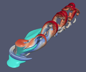
In figure 3, vortex structures are illustrated by means of  $\lambda _2$ isosurfaces (Jeong & Hussain Reference Jeong and Hussain1995). Here, a complete pair of counter-rotating cylinders is shown for case $\varOmega _u=1.5$ to illustrate the symmetry of the induced vortices, and the rest cases ( $\varOmega _u=0, 0.25, 0.5$) are only presented in the $z$-positive half-plane for comparison. The static case ( $\varOmega _u=0$) can be taken from the lowest panel, where two pairs of counter-rotating vortices are created by the roughness element, i.e. the inner vortex (IV) and the horseshoe vortex (HV). Due to the influence of the neighbouring roughness element, the IV is slightly asymmetric. As the cylindrical roughness starts to rotate ( $\varOmega _u=0.25$), a strong DIV is created. At higher rotation speed, secondary inner vortices (SIV, $\varOmega _u=1.0$) and tertiary vortices (TV, $\varOmega _u=1.5$) are created. The generation of the vortical system can be explained in the following way: since the cylindrical element rotates at a constant angular velocity in the boundary layer, a locally accelerated oblique flow is created close to the bottom wall which travels in the spanwise direction to the other side of the cylinder and thereafter creates the DIV. A more detailed discussion of the generation of this vortical system can be found in Wu et al. (Reference Wu, Axtmann and Rist2021).

Figure 3. Vortex visualisation for isolated roughness element ( $Re_{kk}=465.8$, $\eta =1$, $x_k=99.2$) by means of $\lambda _2$, coloured by streamwise velocity $u$. HV, horseshoe vortex; IV, inner vortex; DIV, dominating inner vortex; SIV, secondary inner vortex; TV, tertiary vortex. Red arrows indicate rotation direction. Dashed line indicates the symmetry plane of the counter-rotating cylinder pair with $\varOmega _u=1.5$. Horizontal solid dark lines separate cases.
Figure 4(a–d) depicts another major feature of the steady flow result from the rotating cylinder stub, i.e. the reversed-flow region, as visualised by  $\bar {u}=0$. As shown in figure 4(a), an upstream and a downstream area of reversed flow is typical for boundary-layer flow with static cylindrical roughness elements (Baker Reference Baker1979), i.e. $\varOmega _u=0$. Once the cylinder rotates, a very thin layer of reverse flow covering the upwind half of the cylinder is created, while the downstream reverse-flow region is slightly tilted towards that side at low rotation speed $\varOmega _u=0.25$, see figure 4(b). At higher rotation speed $\varOmega _u=1.0$ in figure 4(c), the downstream reverse-flow region is compressed into a tube-like structure which is connected to a protruding structure at the upwind side of the cylinder. This protruding structure becomes more distinct for $\varOmega _u=1.5$ in figure 4(d).

Figure 4. Visualisation of upstream and downstream reversed-flow regions by  $\bar {u}=0$ isosurfaces for (a) $\varOmega _u = 0$, (b) $\varOmega _u = 0.25$, (c) $\varOmega _u = 1.0$, (d) $\varOmega _u = 1.5$. Curved arrow indicates rotation direction. Streamwise vortices at $x=0$ visualised by grey LIC for cases (e) $\varOmega _u = 0.75$, ( f) $\varOmega _u = 1.0$, (g) $\varOmega _u = 1.25$, (h) $\varOmega _u = 1.5$, coloured by streamwise gradient $\partial u / \partial x$. Thin dashed magenta lines are isolines of $u_x = {-0.3,0.3,0.5,0.7,0.95}$. Red points mark saddle points. Here, red arrows point to separating protruding structures. Black arrows to the emergence of secondary streamwise vortices above and below these protruding reverse-flow regions. Downstream slices at $x=40$ in the last row show flow topology coloured by $u$ for cases (i) $\varOmega _u = 0$, ( j) $\varOmega _u = 0.75$, (k) $\varOmega _u = 1.5$. Thick cyan lines visualise high shear stress regions by means of the $I_2$-criterion (Meyer Reference Meyer2003).
Figure 4(e–h) demonstrates the formation of this protrusion with LIC (line integral convolution, Cabral & Leedom Reference Cabral and Leedom1993; Loring, Karimabadi & Rortershteyn Reference Loring, Karimabadi and Rortershteyn2014) visualisation of the flow field at slice  $x=0$. The grey contours depict the streamwise vortices, which are blended with the streamwise gradient $\partial u/ \partial x$. With the current colour bar, the positive region is hardly discernible due to low amplitude, whereas the regions with negative gradient become distinct. Although the thin reverse-flow region forms on the upwind half of the cylinder stub as long as it rotates ( $\varOmega _u>0$), the protrusion structure does not appear until $\varOmega _u=0.75$ in figure 4(e). At $\varOmega _u=1$, it emerges at $y \approx 0.8$. Secondary streamwise vortices are observed above and below the protruding structure, which are indicated by black arrows and resemble Taylor–Couette vortices between two rotating long cylinders (Taylor Reference Taylor1923). As the cylinder stub rotates at higher angular speed ( $\varOmega _u=1.25, 1.5$), this pair of vortices becomes stronger in figure 4(g,h), respectively. Meanwhile, the region around the reverse-flow region is greatly decelerated, as shown by the pseudocolour, i.e. $\partial u / \partial x$. As the protrusion structure emerges and grows, the highly decelerated region gets concentrated around it. As is known from investigations such as that of Gad-El-Hak et al. (Reference Gad-El-Hak, Davis, Mcmurray and Orszag1984), boundary layer instability is typically promoted by deceleration.
Further downstream, the fundamental topological differences between static and rotating cases are illustrated in figure 4(i–k), which are exemplarily at  $x=40$. For the static case $\varOmega _u=0$, the counter-rotating HV pairs created by each roughness element are evident, whereas for rotating cases ( $\varOmega _u=0.75$, 1.5) the DIV pairs generated by the rotation dominate the streamwise cuts. A crescent of high shear stress region around the DIV (identified by the $I_2$-criterion of Meyer Reference Meyer2003) is noticeable, where inflectional points of the velocity profile are located and consequently inviscid inflectional instability could be expected (Wu et al. Reference Wu, Axtmann and Rist2021).
The influence of rotation on the generation of such vortices can be analysed with the vorticity transport equation:
 \begin{equation} \frac{\partial \boldsymbol{\omega} }{\partial t} ={-}(\boldsymbol{u}\boldsymbol{\cdot}\boldsymbol{\nabla})\boldsymbol{\omega} + (\boldsymbol{\omega} \boldsymbol{\cdot} \boldsymbol{\nabla})\boldsymbol{u} + \nu(\nabla^2 \boldsymbol{\omega}) , \end{equation}
where the right-hand-side terms contain convection, production and dissipation, respectively. The production term can be further decomposed into stretching and tilting terms. The production of streamwise vorticity  $\omega _x$ is decomposed as an example:
 \begin{equation} (\omega_x \boldsymbol{\cdot} \boldsymbol{\nabla})\boldsymbol{u} = \omega_x \frac{\partial u}{\partial x} + \omega_y \frac{\partial v}{\partial y} + \omega_z \frac{\partial w}{\partial z}, \end{equation}
where the first right-hand term is the stretching term and the other two right-hand terms are the tilting terms. The same approach has been used to analyse a porous roughness element in Axtmann (Reference Axtmann2020).
Figure 5 shows the wall-normal projection of the local maximum vorticity production  $\max (P_{\omega _i}(x,z))|_y$ for three cases, i.e. $\varOmega _u=0$, 0.75 and 1.5. For the static case ( $\varOmega _u=0$), the local production maxima for vorticity production in $x,y$ and $z$ directions are symmetric, and they appear at the front edge of the cylinder. As the roughness element rotates, the production terms are no longer symmetric and their maxima extend to the cylinder top. The vorticity production in the near wake is also enhanced, although its magnitude is secondary compared with that in the cylinder region.

Figure 5. Wall-normal projection of local maximum vorticity production. Top row,  $\varOmega _u=0$; middle row, $\varOmega _u=0.75$; bottom row, (c) $\varOmega _u=1.5$. Left column, streamwise production $P_{\omega _x}$; middle column, wall-normal production $P_{\omega _y}$; right column, spanwise production $P_{\omega _z}$. Note that the colour bar consists of a linear part ( $\mathopen |P_{\omega i}\mathclose |\leq 1\times 10^{-2}$) and a logarithmic part ( $\mathopen |P_{\omega i}\mathclose | > 1\times 10^{-2}$) to capture the otherwise imperceptible production in case $\varOmega _u=0$.
The overall effect of rotation on the vorticity budget is evaluated by volume integrals in the streamwise range  $-2\leq x \leq 10$, as shown in figure 6. Here, the constituent parts of the vorticity production, i.e. stretching and tilting terms, are also presented. It is obvious that the convection effect makes almost no contribution to the growth of vorticity in all three directions. The streamwise production $P_x$ grows almost linearly with the rotation speed in the range $\varOmega _u< 1.0$, and then decays gradually from $\varOmega _u> 1.5$, see figure 6(a). In the linear growth range, the production term is mostly caused by streamwise stretching. Beginning from $\varOmega _u = 1.5$, both the magnitudes of stretching and tilting grow significantly, however, the negative tilting effect counteracts the positive contribution of stretching to the production of $\omega _x$. The viscous dissipation grows slowly with increasing $\varOmega _u$ at a low magnitude. Figure 6(b) shows that both stretching and tilting contribute to the production of the wall-normal vorticity $\omega _y$. However, the viscous dissipation grows at the same pace. As a result, the total contribution remains at a low level. The spanwise vorticity budget terms, as shown in figure 6(c), are several magnitudes lower than the streamwise and wall-normal counterparts, and are hence unimportant.

Figure 6. Volume integral of vorticity budget terms in the (a)  $x$-direction, (b) $y$-direction and (c) $z$-direction, non-dimensionalised by the corresponding dissipation $D_i$ of case $\varOmega _u =0$. Here, $P$, production; $Str$, stretching; $Tilt$, tilting; $Cv$, convection; $D$, dissipation terms of vorticity budgets.
The DIV-induced velocity streak is effective in pulling high-speed fluid towards the wall and pushing low-speed fluid to the outer region of the boundary layer, i.e. the lift-up effect (Landahl Reference Landahl1980). Following the definition of Groskopf & Kloker (Reference Groskopf and Kloker2016), the amplitude of velocity streaks is quantified as
 \begin{equation} u_{st}(x) = \tfrac{1}{2}\left(\max_{yz}[u(x,y,z)-\langle u \rangle(x,y)] -\min_{yz}[u(x,y,z)-\langle u \rangle(x,y)]\right) , \end{equation}
where  $\langle u \rangle$ is the spanwise mean value, which represents the three-dimensional base-flow deformation caused by the low- and high-speed streaks. In figure 7, the streak amplitude $u_{st}$ is presented along with the velocity gradient $\boldsymbol {\nabla } u$ maxima, streamwise vorticity $\omega _x$ maxima and spanwise velocity $w$ maxima in $y$–
$y$– $z$ planes. For the velocity gradient, the gradients of streamwise velocity $u$ are emphasised in bold to highlight their dominance of the wall-normal $\partial u/ \partial y$ and spanwise $\partial u/ \partial z$ terms. In general, all the presented parameters are promoted by rising rotation speed $\varOmega _u$, especially in the near wake. Meanwhile, they all reach saturation at $\varOmega _u=0.75{-}1.0$ at around $x\approx 50$. The saturation is probably influenced by the neighbour DIV pairs. As illustrated in figure 4(k), the DIV pairs have been pushed almost to the spanwise boundaries at streamwise station $x=40$ for case $\varOmega _u=1.5$. It can also be observed that, whereas the $\max (\boldsymbol {\nabla } u)|_{yz}$, $\max (\omega _x)|_{yz}$ and $\max (w_x)_{yz}$ decay in the downstream direction, the streak amplitude $u_{st}$ persists for a long streamwise extent. No tendency of decay can be observed within $x<170$ for the saturated curve. With further increase of the rotation speed beyond the saturation case $\varOmega _u=0.75$, the velocity streak amplitude $u_{st}$ becomes oscillatory. Note that the streak amplitude can reach a maximum of 50 % in the near wake, and a maximum of 35 % in the far wake. For comparison, the maximum streak amplitude created by the wing-type miniature vortex generators in (Fransson & Talamelli Reference Fransson and Talamelli2012; Shahinfar et al. Reference Shahinfar, Sattarzadeh, Fransson and Talamelli2012) is 32 %.

Figure 7. Evolution of (a) streamwise base-flow gradient maxima in  $y$–
$y$– $z$ planes, (b) velocity streak amplitude $u_{st}$, (c) streamwise vorticity $\omega _x$ maxima in $y$–
$y$– $z$ planes and (d) spanwise velocity $w$ maxima in $y$–
$y$– $z$ planes. In (a), components of $\boldsymbol {\nabla } u$ are distinguished by different markers. Shaded regions mark extent of the cylindrical roughness. Note that the $x$-axis is a combination of linear ( $x \leq 10$) and logarithmic regions ( $x>10$).
4. Controlled transition
In this section, results of the laminar–turbulent transition controlled by gradually increasing the rotation speed  $\varOmega _u$ of the cylinder stubs around their central, wall-normal axis are presented. Here, only the long-term behaviour of the flow under the influence of numerical background noise is discussed, transient effects are not considered.
4.1. Bifurcation diagram
In order to investigate the dynamic behaviour as the rotation speed  $\varOmega _u$ of the cylinder increases, the perturbation velocities ( $u', v', w'$) at downstream locations are recorded. As the DIV rotates with increasing cylinder rotation rate $\varOmega _u$, the perturbation's maximum in the $y$–
$y$– $z$ plane changes its spatial location accordingly. Therefore, in figure 8 the maximum streamwise velocity perturbation $u'$ at $x=10$ is presented. Three distinctive dynamical regions are identified: laminar ( $0 < \varOmega _u \leq 0.65$), transitional ( $0.65 \leq \varOmega _u \leq 1.31$) and chaotic ( $\varOmega _u \geq 1.375$). The corresponding flow features at different stages of transition are visualised by instantaneous contours of streamwise velocity $u$, as shown in figure 9. It is found that, below $\varOmega _u = 0.65$, the flow is stable and remains laminar despite a certain level of initial perturbations. The laminar flow is featured by stable velocity streaks with a high-speed streak in the centre, see figure 9(a). Beginning from the critical rotation speed $\varOmega _u^c = 0.65$, a self-sustained global instability is observed. The grey line in figure 8 is the best least-squares fit using $\sqrt {\varOmega _u - \varOmega _u^c}$ as the fitting function. This means that an increase of the cylinder rotation speed results in a supercritical Hopf bifurcation. The equilibrium state in the low $\varOmega _u$ region is broken and turns into a periodic limit-cycle oscillation at $0.65 \leq \varOmega _u \leq 1.31$. The transitional flow is characterised by braid-like structures between the low- and high-speed steaks, resembling the K–H instability, see figure 9(b). Interestingly, the boundary layer relaminarises in the range of $1.06 \leq \varOmega _u \leq 1.25$. Although the streamwise velocity perturbation at $x=10$ for $\varOmega _u=1.0$ is still larger than that for $\varOmega _u=0.75$, the overall relaminarisation effect is already distinctive, leaving the braid-like structure confined to the near-wake region, see figure 9(c). On further increase the rotation speed to $\varOmega _u=1.25$ in figure 9(d), the perturbation structure near the cylinders recedes to an almost imperceptible level. However, the perturbation amplitude for case $\varOmega _u >1.25$ climbs rapidly to follow the least-squares fitted level. The near-wake flow structure of case $\varOmega _u= 1.31$ in figure 9(e) is similar to that of case $\varOmega _u= 1.0$. With a further increase of the rotation speed to $\varOmega _u= 1.375$, the flow becomes chaotic. In figure 9( f), the regular braid-like patterns in both the near wake and far wake are broken, indicating that laminar–turbulent transition has already happened.

Figure 8. Bifurcation diagram of the global instability for  $Re_{kk} =465.8$. Perturbation data obtained at $(x,y,z) = (10, 1, 2)$. Solid grey line represents best least-squares fit. Dashed line represents unstable equilibrium. The dash-dotted and dotted lines for $\varOmega _u \geq 1.0$ are unrelated to the dynamics; their purpose is to connect data.

Figure 9. Instantaneous contours of streamwise velocity  $u$ at $y = 0.99$: (a) $\varOmega _u=0.25$, (b) $\varOmega _u=0.75$, (c) $\varOmega _u=1.0$, (d) $\varOmega _u=1.25$, (e) $\varOmega _u=1.31$, ( f) $\varOmega _u=1.375$. Yellow curves in the near wake ( $x\leq 3$) indicate reverse-flow regions.
Figure 10 shows phase portraits of the perturbation velocities at probe location  $(x,y,z) = (20,1,2)$, and the corresponding PSD of the streamwise perturbation velocity $u'$ for several characteristic $\varOmega _u$, as already used in figure 9. The cases $\varOmega _u = 0.25$ and $\varOmega _u = 1.25$ are illustrated in figures 10(a,b) and 10(g,h), where a fixed point in the phase portrait indicates that the flow is in a steady state. Although the perturbations in both cases are not absolutely zero, the dynamical energies as exhibited in the PSD are negligible. For $\varOmega _u = 0.75$, an ‘8’-shaped limit cycle in the phase portrait and a fundamental frequency ( $\omega _1 \approx 0.9$) accompanied by its higher harmonics in the PSD plot indicate that the system undergoes a periodic limit-cycle oscillation. The rapid rise of perturbation $u'$ at $1.26< \varOmega _u<1.285$ in figure 8 is the result of a period-halving bifurcation and an amplification of the higher-harmonic components, as displayed in figures 10(i,j) and 10(k,l). It will be discussed in § 4.2 that the primary frequency $\omega _1$ is associated with hairpin vortex shedding induced by the rotating cylinders and the higher harmonics are an indication of nonlinear effects. At rotation speed $\varOmega _u = 1.31$, a second frequency $\omega _2 = 0.47$ begins to emerge in figure 10(n), albeit of low PSD magnitude. The incommensurate frequencies ( $\omega _2 / \omega _1$ is irrational) lead to a quasi-periodic motion of the perturbations, turning the limit cycle into a limit torus in figure 10(m). Further increasing the rotation speed to $\varOmega _u = 1.375$, a cascade of period-halving and period-doubling bifurcations led to a chaotic attractor of the phase portrait in figure 10(o). Its PSD spectrum is dominated by the second basic frequency $\omega _2 = 0.465$.

Figure 10. Three-dimensional phase portraits of perturbations ( $u', v', w'$) and their corresponding PSD at probe location $(x,y,z)=(20, 1, 2)$; (a,b) $\varOmega _u=0.25$, (c,d) $\varOmega _u=0.75$, (e,f) $\varOmega _u=1.0$, (g,h) $\varOmega _u=1.25$, (i,j) $\varOmega _u=1.2673$, (k,l) $\varOmega _u=1.285$, (m,n) $\varOmega _u=1.31$, (o,p) $\varOmega _u=1.375$. Colours in phase portraits vary with sampling time.
The dynamic behaviour of the perturbations as they evolve spatially is presented in figure 11. The transitional case  $\varOmega _u=1.31$ is compared with the chaotic case $\varOmega _u=1.375$. For $\varOmega _u=1.31$, its closed loop phase portrait in figure 11(a) and the single dominant frequency $\omega _1=1.81$ at $x=1$ in figure 11(b) indicate that the perturbations undergo a period-1 limit-cycle oscillation. As the flow evolves downstream, the local perturbations undergo a period-halving bifurcation at $x=10$, resulting in the amplification of higher harmonics $2\omega _1$ and $3\omega _1$. Further downstream at $x=40$, a quasi-periodic oscillation of the perturbation is identified by the appearance of a second and a third frequency $\omega _2 = 0.465$ and $\omega _3 = 2.28$, respectively, in figure 11(j) and the limit torus in the phase portrait of figure 11(i). At $x=90$, the dominating frequency of the perturbations transits to the secondary mode $\omega _2$ in figure 11(n). The incommensurate frequencies turn the phase portrait into a non-overlapping limit torus in figure 11(m), while the primary frequency $\omega _1$ declines to an almost unnoticeable level, indicating a changeover of the flow feature from the near-wake vortex shedding to a low-frequency secondary instability in the far wake. Whereas for case $\varOmega _u=1.375$, the strange attractor at $x=1$ in figure 11(c) implies that the system experiences a chaotic motion in the very near wake, nevertheless, its PSD in figure 11(d) is still dominated by the primary frequency $\omega _1= 1.81$, which is related to vortex shedding, along with low energy harmonic $2\omega _1$ and low frequency component modulations. As the flow evolves to $x=10$, a cascade of period-doubling and period-halving bifurcations of the local perturbations are observed, which bring about the energy amplification of higher harmonic $2\omega _1$, a second frequency $\omega _2$ and a third frequency $\omega _3$, as shown in figure 11(h). In addition to its fractal structure in the phase portrait which is still observable in figure 11(g), the orbit is blended by irregular loops, demonstrating the chaotic nature of the perturbations. At $x=40$, a tertiary instability identified by $\omega _3$ dominates the PSD spectrum in figure 11(l), whereas the primary frequency $\omega _1$ diminishes. Further downstream, the discrete frequency spectrum converges rapidly to a continuous one in figure 11(p), indicating an evolution of the aforementioned quasi-periodic deterministic perturbations into a turbulent state (Borodulin & Kachanov Reference Borodulin and Kachanov2013).

Figure 11. Three-dimensional phase portraits of perturbations ( $u', v', w'$) and their corresponding PSD at different probe locations: 1st row, $(x,y,z)=(1, 1, 2)$; 2nd row, $(x,y,z)=(10, 1, 2)$; 3rd row, $(x,y,z)=(40, 1, 2)$; 4th row, $(x,y,z)=(90, 1, 2)$. Left columns (a,b,e,f,i,j,m,n) $\varOmega _u=1.31$; right columns (c,d,g,h,k,l,o,p) $\varOmega _u=1.375$. Colours in phase portraits vary with sampling time.
Typically, laminar–turbulent transition is accompanied by an increasing drag coefficient. Figure 12 shows the streamwise evolution of the skin-friction coefficient  $C_f = 2 \tau _{wall} / (\rho u^2_\infty )$ for various rotation speeds $\varOmega _u$. The three dynamical regions as distinguished in figure 8 are marked by contrasting colours. For laminar cases ( $\varOmega _u = 0, 0.25, 0.46$), $C_f$ rises behind the roughness elements and decays gradually after reaching a mild peak at around $x= 20 \sim 30$. The transitional cases ( $\varOmega _u = 0.65 \sim 1.25$) are characterised by a two-peak wavy progression of $C_f$, with the first peak at around $x\approx 5$ and the second peak at around $x\approx 20$. Starting from the near wake, the skin-friction coefficients of chaotic cases ( $\varOmega _u \geq 1.375$) rise monotonically towards the value of a turbulent boundary-layer correlation. Here, the $1/7$ power law with experimental calibration (Schlichting & Gersten Reference Schlichting and Gersten2003) is given for reference. The different qualitative features of the skin-friction coefficient $C_f$ evolution substantiate the aforementioned categorisation of the boundary-layer flow, and are a consequence of symmetry breakings in the evolution of the vortical systems induced by the rotating cylindrical roughness elements.

Figure 12. Streamwise evolution of skin-friction coefficient  $C_f$ compared with $1/7$ power law with experimental calibration (Schlichting & Gersten Reference Schlichting and Gersten2003). Colour of the plots are kept in accordance with figure 8: blue (laminar), red (transitional), black (chaotic). Note that the $x$-axis is a combination of linear ( $x \leq 10$) and logarithmic regions ( $x>10$).
4.2. Instantaneous flow-field structures
Having discussed the dynamic behaviour of the perturbations, the instantaneous flow structures as visualised by isosurfaces of  $\lambda _2$ (Jeong & Hussain Reference Jeong and Hussain1995) will be analysed in this section. Figure 13 shows instantaneous snapshots of vortices emanating from the cylinders at a dimensionless rotation speed of $\varOmega _u=0.75$. The depicted frames denote the positions where the near-wake regions are extracted, and are shown in figure 14. For illustration purposes, an additional half-unit of the flow domain is added at $z>6$. The vortices obtained with SFD, which remain laminar, are included in blue colour for reference. In the very near wake ( $x\leq 5$), the instantaneous vortices almost overlap with the laminar base-flow vortices. The flow is characterised by a DIV surrounded by a SIV, as shown in the enlarged figure 14. Unsteady behaviour appears first on the SIV at around $x\approx 5$, it develops into a tiny hairpin vortex with its head rotated around the DIV, which decays quickly at around $x=23$. Wavy structures are observed on the DIV from $x\approx 5$ as well, and the DIV meanders in the direction normal to the streamwise direction. Such a meandering dynamics is well reported in the initial stage of hairpin vortex generation (Schoppa & Hussain Reference Schoppa and Hussain2002; Wang, Huang & Xu Reference Wang, Huang and Xu2015). Slightly downstream at $x \approx 23$, an arch-shaped structure forms, which is tilted towards the high-speed streak. Its stronger leg is rooted in the DIV and its weaker leg stretches towards the low-speed streak. The slight cross-flow $w$ induced by the DIV, as shown in figure 7(d), pushes the tilted hairpin vortex packets away from the centre high-speed region. Thus, they merge at the spanwise boundary with the neighbour packets at $x\approx 50$, see figure 13. Further downstream, higher harmonics are triggered and quasi-streamwise vortices are generated. Another vortex combines at the periodic boundary and then evolves into a new packet of hairpin vortices at $x\approx 72$. Since the spanwise velocity $w$ is cancelled out by the neighbouring vortices here, this new hairpin vortex is symmetric with legs of identical strength. The primary frequency $\omega _1$, as plotted in figure 10(d), therefore, corresponds to the periodic shedding of the tilted hairpin vortices. Moreover, it turns out that the frequency and wavelength of the near-wake tilted hairpin vortex packet are identical to those of the far-wake symmetric hairpin vortex. In addition, the ejection ( $Q2$,
$Q2$,  $u'<0$, $v'>0$) and sweep ( $Q4$,
$Q4$,  $u'>0$, $v'<0$) events of a hairpin vortex are shown as well (Adrian Reference Adrian2007). The strength of both $Q2$ and $Q4$ events grows in the streamwise direction, proving that the hairpin vortex generation for this case is a streak-instability-based scenario (Schoppa & Hussain Reference Schoppa and Hussain2002). As shown in figure 14(a), the interaction of DIV and SIV in the near wake ( $x \leq 25$) resembles the dynamics of a vortex pair (Leweke, Le Dizes & Williamson Reference Leweke, Le Dizes and Williamson2016), where a short wave 3-D elliptic instability (Kerswell Reference Kerswell2002) is responsible for the breakdown into turbulent motion.

Figure 13. Instantaneous isosurface of flow pattern for case  $\varOmega _u=0.75$ by means of $\lambda _2=-200$, coloured by streamwise velocity $u$. (a) Top view, ejection ( $Q2$, coloured yellow) and sweep ( $Q4$, coloured green) events are shown by $u'v' = -0.003$, (b) side view. Depicted frames are enlarged in figure 14.

Figure 14. Enlarged views of the frames in figure 13. (a) Perspective view, (b) top view and (c) side view. Red curve indicates the rotation direction.
The instantaneous flow organisation of case  $\varOmega _u=1.31$, which is closer to a chaotic state, is shown in figure 15. For clarity, the near-wake region is also enlarged in figure 16. As discussed above, the hairpin vortices for case $\varOmega _u= 0.75$ shed from the quasi-steady DIV. Here, the hairpin vortex is generated directly on the decelerating side of the rotating cylindrical roughness elements and regenerates into a hairpin packet. The hairpin packet has an interlaced structure which clearly proves its parent–offspring origin (Zhou et al. Reference Zhou, Adrian, Balachandar and Kendall1999), i.e. hairpin vortices are regenerated from the preceding parent hairpin vortex. The accompanying $Q2$ and $Q4$ events confirm their regeneration mechanism as well. The enlarged views in figure 16 clearly show the spatial organisation of the hairpin vortex packet. The mean reverse-flow zone, as shown by $\bar {u}_x=0$, has a structure protruding into the decelerated boundary layer at height $y=0.6 \sim 0.85$, see the enlarged side view in figure 16(c). This protrusion splits the unsteady vortex on the decelerated side into two parts, which then develop into streamwise oriented legs of the first hairpin vortex. Due to a K–H instability, the inflectional shear flow rolls up into a spanwise vortex which bridges the two legs and forms the hairpin head. The local ejection events near the head and legs of the first hairpin vortex then regenerate the next pair of legs, thereafter an offspring hairpin vortex is created. Further downstream, this hairpin packet gradually decays, whereas a low-frequency hairpin starting at $x\approx 68$ is formed with its two legs rising from neighbouring units, see figure 14(a). It is to be noted that these far-wake low-frequency hairpin vortices exhibit asymmetry, i.e. symmetry breaking, which is a precursor of chaos.

Figure 15. Instantaneous isosurface of flow pattern for case  $\varOmega _u=1.31$ by means of $\lambda _2= -200$, coloured by streamwise velocity $u$. (a) Top view, ejection ( $Q2$, coloured yellow) and sweep ( $Q4$, coloured green) events are shown by $u'v' = -0.003$, (b) side view. The mean reverse-flow zone $\bar {u}_0=0$ is marked by cyan colour. Depicted frames are enlarged in figure 16.

Figure 16. Enlarged views of the frames in figure 15. (a) Perspective view, (b) top view and (c) side view. Red curve in (b) indicates the rotation direction.
The flow statistics of the chaotic cases ( $\varOmega _u = 1.5, 2$) are presented together with mean-flow profiles in figure 17. The streamwise mean-flow velocity profiles, which are non-dimensionalised by $\bar {u}^+=\bar {u} / u_\tau$ with regards to wall coordinate $y^+= y u_\tau / \nu$, are given in figure 17(a,d). The theoretical curves for the viscous sublayer $\bar {u}^+ = y^+$ and the logarithmic layer $\bar {u}^+ = 1/\kappa \ln y^+ +C$ with $\kappa = 0.41$ and $C=5.2$ are plotted with dashed lines. For reference, the fully developed turbulent data of Schlatter & Örlü (Reference Schlatter and Örlü2010) are depicted with solid red lines as well. The mean-flow profiles of both cases evolve gradually towards a turbulent one, with case $\varOmega _u = 1.5$ in an oscillatory manner and case $\varOmega _u = 2$ in a gradual manner. The streamwise components of Reynolds normal stress $\tau ^+_{xx}$ as well as shear stress $\tau ^+_{xy}$ are given. At $x=1$, a very high peak of both Reynolds stresses is observed at height $y^+= 30$, which corresponds to the height of the cylinder. For the streamwise normal stress $\tau _{xx}$, this peak quickly decays and shifts to $y^+= 45$ at station $x= 10$. Further downstream at $x=20$, a second peak appears and grows in height $y^+\approx 13$. Whereas this location conforms to the peak of the fully developed turbulence, the magnitude grows to approximately two times larger at $x=100$. For the shear stress $\tau ^+_{xy}$, the peak at $y^+= 30$ gradually spreads out towards the fully developed turbulent profile.

Figure 17. Evolution of mean velocity profiles (a,d) and turbulence statistics (b,c,e,f) along streamwise direction. Upper row corresponds to case  $\varOmega _u = 1.5$ and lower row to case $\varOmega _u = 2$. Red solid line is from DNS data of Schlatter & Örlü (Reference Schlatter and Örlü2010). For clarity, shear stresses of near-wake ( $x \leq 20$) and far-wake ( $x \geq 40$) locations are plotted with offset.
4.3. DMD analysis
In this section, the transitional flows controlled by the rotating cylindrical roughness elements are investigated by DMD (Schmid Reference Schmid2010; Belson et al. Reference Belson, Tu and Rowley2014). The spatio-temporal process of the 3-D boundary-layer flow can be decomposed into a set of coherent spatial modes which feature corresponding frequencies. At high rotation speed, nonlinear modal interactions can develop. In such a case, the resulting DMD mode should be interpreted as one particular representative phase-dependent dynamical mode determined by the nonlinear interactions of the snapshots employed. In low rotation speed cases, however, such nonlinear effects can be neglected. The obtained DMD modes are therefore identical to a global mode as obtained from a global stability analysis (Loiseau et al. Reference Loiseau, Robinet, Cherubini and Leriche2014). Since only the asymptotic behaviour of the perturbations are considered in the current work, DMD is performed with equilibrium state snapshots. Approximately 200 snapshots are used to perform DMD for the investigated cases, which results in a temporal sampling rate that is more than twice the highest dominant frequency of instability. Figure 18(a) shows the complex DMD eigenvalues for case  $\varOmega _u= 1.31$. Here, almost all modes are located on the unit circle by virtue of the equilibrium flow state. The few low amplitude modes inside the unit circle are most likely nonlinearly generated higher harmonics and numerical artefacts. The non-dimensional physical frequency $\omega _r$ and its corresponding mode amplitude coefficients $a_i$ are plotted in figure 18(b). The primary frequency $\omega _1$ and its higher harmonics as well as the second frequency $\omega _2$ as shown in figure 11 are recovered by DMD.

Figure 18. The DMD spectrum of case  $\varOmega _u = 1.31$. Colour and size in (a) are related to coefficient amplitude. (a) Complex eigenvalues $\lambda$ and (b) amplitudes of DMD modes.
Figure 19 shows the leading DMD modes of the selected cases from the bifurcation diagram in figure 8. The modes consist of positive and negative patches of velocity mostly localised around the central low-speed region, i.e. the DIV structure in the laminar cases. In case  $\varOmega _u = 0.75$, the leading DMD mode is a low-frequency spatially growing mode, whose mode amplitude is shown in figure 25(b,c) in Appendix A to saturate at $x\approx 50$. For $\varOmega _u = 1.0$, the leading DMD mode is a high-frequency mode which fades away after $x=50$, whereas the DMD mode for the relaminarised case $\varOmega _u = 1.25$ only emerges in the far wake ( $x\approx 50$). It is to be noted that the amplitude of the leading mode in $\varOmega _u = 1.25$ is several orders of magnitude lower than the DMD modes of other cases. Further increase of the rotation speed to $\varOmega _u = 1.31$ leads to the occurrence of two leading DMD modes as shown in figure 18, i.e. a high-frequency mode (coloured red/blue, $\omega _1=1.8$) in the near wake and a low-frequency mode (coloured white/black, $\omega _2=0.47$) in the far wake. The asymmetrical spatial structure of the low-frequency mode implies the onset of chaotic flow.

Figure 19. Real part of dominant DMD modes. Frequencies for each mode: (a)  $\omega _r=0.92$, (b) $\omega _r=2.2$, (c) $\omega _r=0.66$, (d) primary mode $\omega _1=1.8$ with isosurface in red/blue and second mode $\omega _2=0.46$ with isosurface in white/black. Isosurfaces depict $\hat {u}= \pm 10\,\%$ (in colour red/blue or white/black) of maximum amplitude of mode.
The structures of the leading modes and their spatial locations relative to the mean flow are visualised in slices at  $x=10$ in figure 20. Here, only the positive- $z$ half of the modes is shown due to the symmetry of the DMD modes with regard to the $z=0$ axis. The 3-D high shear region is identified by the $I_2$-criterion (Meyer Reference Meyer2003). For cases $\varOmega _u = 0.75, 1.0, 1.25$, the mean flow is characterised by a tilted high shear region surrounding the strong streamwise vortex, i.e. the DIV. Typical instability modes behind a static cylindrical roughness element can be categorised by their spanwise symmetries, i.e. varicose or sinuous, with respect to the vertical axis where the cylinder is located. As shown in figure 20, such spanwise symmetrical characteristic is no longer a feature of the induced modes. Nevertheless, the DMD modes presented here are exclusively located within the high shear stress regions, indicating their inflectional nature. Similarly tilted modes are observed with skewed (oblique) roughness elements in Groskopf & Kloker (Reference Groskopf and Kloker2016), with distributed surface roughness in Di Giovanni & Stemmer (Reference Di Giovanni and Stemmer2018) and more intensively with cross-flow instability in Malik, Li & Chang (Reference Malik, Li and Chang1994); Wassermann & Kloker (Reference Wassermann and Kloker2002) and Shi, Mader & Martins (Reference Shi, Mader and Martins2021). As for case $\varOmega _u = 1.31$, the mean flow has already been distorted by the interaction of its leading modes, which are identified in figure 18.

Figure 20. Real part of leading DMD modes with primary frequency  $\omega _r$ in $x=10$ plane shown by red/blue contours for cases (a) $\varOmega _u= 0.75$, (b) $\varOmega _u= 1.0$, (c) $\varOmega _u= 1.25$, (d) $\varOmega _u= 1.31$. Red/blue contours show positive/negative values of normalised spatial eigenfunction. Thin dash-dotted lines are isolines of mean streamwise velocity $\bar {u} = 0.1{-}0.99$. Thick cyan solid lines visualise high shear stress regions by means of $I_2$-criterion (Meyer Reference Meyer2003).
4.4. Instability mechanisms
The PKE analysis is performed to get an insight into the instability mechanisms for the above identified DMD modes, particularly, how the modes obtain their energy from the work of Reynolds stress against the mean-flow shear. Figure 21 presents the streamwise evolution of perturbation productions  $\int _{y,z} I_i \,\textrm {d}y\,\textrm {d}z$ scaled by the local dissipation $\int _{y,z} |D| \,\textrm {d}y\,\textrm {d}z$. The purpose is to magnify the otherwise imperceptible energy production at the initial stage of the instability. It is evident that the energy production is dominated by the $\int _{y,z} I_2 \,\textrm {d}y\,\textrm {d}z$ and $\int _{y,z} I_3 \,\textrm {d}y\,\textrm {d}z$ terms for almost all cases, which is reasonable and common for a streaky boundary layer, see Cossu & Brandt (Reference Cossu and Brandt2004), Loiseau et al. (Reference Loiseau, Robinet, Cherubini and Leriche2014) and Wu et al. (Reference Wu, Axtmann and Rist2021) as well. However, it should be noted that in the roughness region ( $-0.5 \leq x \leq 0.5$) the term $\int _{y,z} I_1 \,\textrm {d}y\,\textrm {d}z$ dominates the energy production for cases with $\varOmega _u \geq 1.0$. As shown in (2.12), the term $I_1$ represents the production of $e_k$ from the normal Reynolds stress $u'^2$ against the streamwise gradient of the mean-flow streamwise component $\partial \bar {u} / \partial x$. Since the sign of the normal shear $u'^2$ is always positive and the sign for the gradient $\partial \bar {u} / \partial x$ on the reverse-flow side of the cylinder is negative due to the deceleration effect, the production term $I_1$ then turns out to be invariably positive. The mechanism is hereafter termed a deceleration mechanism. The crucial importance of the deceleration effect on intensifying the growth rate of the shear-layer instability has been addressed by Gad-El-Hak et al. (Reference Gad-El-Hak, Davis, Mcmurray and Orszag1984) and Shtern & Hussain (Reference Shtern and Hussain2003).

Figure 21. Streamwise evolution of production terms  $\int _{y,z} I_i / |D| \,\textrm {d}y\,\textrm {d}z$ of leading DMD modes for (a) $\varOmega _u= 0.75$, (b) $\varOmega _u= 1.0$, (c) $\varOmega _u= 1.25$, (d) $\varOmega _u= 1.31$. Dissipation $D$ is plotted at $I_i/D = -1$ for reference. Note that $x$-axis contains linear ( $x \leq 10$) and logarithmic ranges ( $x>10$). Vertical shaded region in the insets indicate the location of cylinders.
The real parts of the leading modes at slice  $x=0$ are shown in the first row of figure 22, the second and third rows represent the local total energy production at slices $x=0.3$ and $x=2$, respectively. For higher rotation speed cases $\varOmega _u = 1, 1.25, 1.31$, both the DMD modes and the local total energy productions $\sum I_i$ are localised around the protruding structures as marked by the reverse-flow region ( $\overline {u}_x=0$), where the deceleration mechanism gives birth to the DMD modes shown in figure 19(b–d). Nevertheless, the total energy production for case $\varOmega _u = 0.75$ is counterbalanced by a positive region (contribution of $I_1$) and a negative region (contribution of $I_3$), which implies a different instability mechanism for the DMD mode as shown in figure 19(a).

Figure 22. Real part of leading DMD modes in  $x=0$ plane shown by red and blue contours for case (a) $\varOmega _u= 0.75$, (b) $\varOmega _u= 1.0$, (c) $\varOmega _u= 1.25$, (d) $\varOmega _u= 1.31$. Thin dash-dotted lines are isolines of mean streamwise velocity $\bar {u} = 0.1-0.99$. Recirculating region is marked by black solid lines. Total local energy production $\sum I_i$ at $x=0.3$ (second row) and $x=2$ (third row) for (e,i) $\varOmega _u= 0.75$, (f,j) $\varOmega _u= 1.0$, (g,k) $\varOmega _u= 1.25$, (h,l) $\varOmega _u= 1.31$. Yellow dash-dot lines mark the phase speed $c_{ph}$ of the corresponding mode. Recirculating regions are marked by magenta thick solid lines. Thin magenta dash-dotted lines are isolines of $\bar {u} = 0.99$. Thick cyan solid lines visualise shear regions by means of $I_2$-criterion (Meyer Reference Meyer2003). Yellow line in (h) for comparison with figure 23(c).

Figure 23. Elliptic flow regions ( $\beta <1$, coloured blue) at $x=2$ for cases (a) $\varOmega _u=0.75$ and (b) $\varOmega _u=1$. Centrifugally unstable regions ( $\gamma <0$, coloured red) at $y=1.07$ for case (c) $\varOmega _u=1.31$. The dashed circle in (c) marks the location of the cylinder. Yellow line in (c) for comparison with figure 22(h).
The third row of figure 22 shows the total energy productions at slice  $x=2$, which is a position across the downstream reverse-flow region. For case $\varOmega _u = 1.31$ in figure 22(l), the flow has curved streamlines around the cylinder and the velocity is decelerated at the region of total energy production, which are flow conditions prone to a centrifugal instability (Floryan Reference Floryan2002; Lanzerstorfer & Kuhlmann Reference Lanzerstorfer and Kuhlmann2012). The argument is supported by the sufficient condition of Sipp & Jacquin (Reference Sipp and Jacquin2000), that a 2-D inviscid flow is centrifugally unstable if the following parameter is negative along a closed streamline $\psi = {\rm const}$.
 \begin{equation} \gamma := \frac{|\bar{\boldsymbol{u}}|\omega }{R} < 0, \end{equation}
where  $\omega$ is the vorticity of the mean flow, and $R$ is the local algebraic radius of curvature, defined as
 \begin{equation} R=\frac{|\bar{\boldsymbol{u}}|^3 }{ \boldsymbol{\nabla} \psi \boldsymbol{\cdot} (\bar{\boldsymbol{u}} \boldsymbol{\cdot} \boldsymbol{\nabla} \bar{\boldsymbol{u}}) }. \end{equation}
Figure 23(c) compares the regions where  $\gamma <0$ at height $y=1.07$ for case $\varOmega _u=1.31$ with the mean flow. It can be observed that negative $\gamma$ occurs in regions of flow divergence and convergence in the tilted wake, exactly at the edges of the vortex train in figure 15(b). The total energy production in figure 22(h) is also observed to overlap with this region. For better comparison, reference spatial locations are marked by a short yellow line in figures 22(h) and 23(c).
The cases with  $\varOmega _u = 0.75$ and $1.0$ are slightly different because the perturbation kinetic energy is produced in two regions: the high shear region as identified by the $I_2$-criterion and the centre of the elliptic vortex of the mean flow, see figure 22(i,j). The latter is an indication of an elliptic instability (Pierrehumbert Reference Pierrehumbert1986; Sipp & Jacquin Reference Sipp and Jacquin1998). This interpretation is supported by the theory of elliptic instability proposed by Pierrehumbert (Reference Pierrehumbert1986) and Waleffe (Reference Waleffe1990), that a strained vortex is subject to elliptic instability if the eccentricity parameter $\beta$ of the flow is less than 1, i.e.
 \begin{equation} \beta := \frac{2\epsilon}{ |\omega| } < 1. \end{equation}
Here,  $\epsilon$ is the magnitude of strain and $\omega$ is the vorticity. Figure 23(a,b) shows the elliptic flow regions at $x=2$ for cases $\varOmega _u=0.75$ and $\varOmega _u=1$, respectively. Further, the maximum of the perturbation, which is located in the crescent-shaped high shear region (see figure 20a,b for instance) and the maximum of perturbation energy production $\sum I_i$ approximately coincide with the location of the critical layers as marked by the phase velocities $c_{ph}$. A criterion that meets the Rayleigh–Fjortøft necessary condition for inviscid inflectional instability (Schmid & Henningson Reference Schmid and Henningson2001). Therefore, the cases $\varOmega _u = 0.75$ and $1.0$ are subject to a combination of inviscid instability and elliptic instability in the near wake. The case for $\varOmega _u=1.25$ in figure 22(k) exhibits the same inviscid instability feature. However, the case is unique in that it is dominated by a relaminarisation effect which is not the topic of the current investigation. In the far wake, both centrifugal and elliptic effects fade away.
5. Conclusions
The transition of a laminar boundary layer controlled by counter-rotating wall-normal cylindrical roughness pairs has been investigated numerically by increasing the rotation speed  $\varOmega _u$ incrementally. Unsteady simulations demonstrate that the boundary layer undergoes a supercritical Hopf bifurcation, as the rotation speed $\varOmega _u$ is gradually increased. The braid-like leading DMD modes, which are located mainly within the crescent-shaped high shear regions, are associated with hairpin vortex shedding. Flow visualisations with $\lambda _2$ isosurfaces have shown that the hairpin vortex regeneration for the low rotation speed case $\varOmega _u = 0.75$ is a streak-instability-based mechanism, and for the large rotation speed case $\varOmega _u = 1.31$ a parent–offspring mechanism. The symmetry breaking which is already observed at $\varOmega _u = 1.31$ eventually triggers transition to turbulence with larger rotation speed. Interestingly, a relaminarisation effect is observed in the rotation range $1.06 \leq \varOmega _u \leq 1.25$, which is probably due to the influence of neighbour vortices and needs further investigation.
Regarding instability mechanisms, a combination of centrifugal instability ( $\varOmega _u= 1.31$) and elliptic instability ( $\varOmega _u= 0.75, 1.0$) in the near wake is found to trigger the DMD mode, while a deceleration mechanism directly located on the upwind side of the rotating cylinder is found to initiate the instability. Unlike the much more common scenario with static cylinders, where the formations of near-wake horseshoe vortices, inner vortices and far-wake velocity streaks are ascribed to blockage effects induced by the roughness elements, the rotating cylinder stubs cause local deceleration on one side of the cylinder and local acceleration on the other side. It turns out that both the downstream macro-scale vortical structures, i.e. the long-lived DIV and the surrounding SIV, and the micro-scale instabilities as well as the consequent transition are related to this local boundary-layer deceleration. A major flow structure, i.e. a protruding reverse-flow region which is created by Taylor–Couette-like streamwise vortices above and below it, forms at the upwind side of the cylinder as the rotation speed increases beyond $\varOmega _u = 1$. The decelerated region is further accumulated around this protruding structure and is found effective in kinetic energy production, which nurtures the flow instability and consequently triggers transition to turbulence.
Overall, the current investigations have presented an active method for flow tripping. A gear-driven rotation apparatus has been constructed in the laminar water channel by the present authors, which demonstrated its feasibility of construction. Technically speaking, micro-rotors rotating at a million rpm are already practicable (Gong & Habetler Reference Gong and Habetler2017), which makes the current flow control method applicable for a wide range of fluid mechanical applications. Furthermore, based on the fact from Wu et al. (Reference Wu, Axtmann and Rist2021) that low rotation cylinder pairs ( $\varOmega \leq 0.5$) can attenuate TS instabilities more effectively than static cylinders, one may also propose to use it for laminar flow control. Moreover, the wall-normal counter-rotating cylindrical roughness pairs are observed in another DNS study to act as micro-vortex generators (MVGs), similar to the winglet-type MVGs of Shahinfar et al. (Reference Shahinfar, Sattarzadeh, Fransson and Talamelli2012) and Lin et al. (Reference Lin, Robinson, McGhee and Valarezo1994). Therefore, this method is also considered applicable to controlling boundary-layer separation in a turbulent flow.
Acknowledgements
Computational resources provided by the federal high-performance computing centre Stuttgart (HLRS) under grant GCS_Lamt (LAMTUR) are kindly acknowledged.
Funding
The authors gratefully appreciated the financial support from the China Scholarship Council (no. 201406280033) and Deutsche Forschungsgemeinschaft under project numbers RI 680/39-1 and RI 680/48-1.
Declaration of interests
The authors report no conflict of interest.
Appendix. Grid convergence study
In this appendix, the influence of the mesh size on the computed instability is highlighted. Two special cases are chosen for the grid convergence study, i.e.  $\varOmega _u = 0.75$ and $\varOmega _u = 1.5$. In case $\varOmega _u = 0.75$, a dominant DMD mode is observed, while the case $\varOmega _u = 1.5$ is a chaotic scenario. Figure 24(a) illustrates the integration domain used for this investigation, and the grid topology around the cylinder is depicted in figure 24(b). The integration domain dimensions $L_y$ and $L_z$ are kept constant (i.e. $L_y = 40$ and $L_z = 12$) for all cases, while the streamwise size is truncated from $L_x=200$ for the coarsest case to $L_x=85$ in the finest case so as to minimise the total cell number. Four grids with refinement in all three directions are studied, as listed in table 1. The cell size of the finest grid G4 is $\Delta y^+_0 =0.15$, $\Delta z^+=1.1$ and $\Delta x^+$ stretches from $\Delta x^+_{min} = 0.15$ near the cylinder to $\Delta x^+_{max} = 2.9$ at the outlet, which results in a total of 112 million cells. For all cases, the integration time steps are adjusted to ensure that the Courant numbers are kept below $Co=0.35$. Flow statistics are evaluated after five flow-through times, which corresponds to $t u_\infty /k=450$ time units. For evaluation of the statistics, a sampling time period of at least $t u_\infty /k \sim 1000$ is used.

Figure 24. (a) Sketch of integration domain. (b) Grid topology around cylinder.
Table 1. Numerical set-ups for grid convergence study.

Figure 25 shows the grid convergence study from case  $\varOmega _u = 0.75$, which is characterised by a dominant DMD mode with $\omega = 0.92$. The natural logarithm of the spatial maximal modal amplitude and the $n$-factor calculated as $n= \ln (|\hat {u}(x)| / |\hat {u}(x_0)|)$ are shown in figures 25(b) and 25(c), respectively. Although the initial amplitudes of this mode are different between grids, the $n$-factors referring to the rear edge of the cylinder overlap with each other in the near wake for all grids. The discrepancy of $n$-factors is only discernible in the far wake, i.e. at $x>20$. Nevertheless, the overlap of grids G3 and G4 in the whole domain confirms the grid convergence.

Figure 25. Results of grid convergence study showing (a) real part of dominant DMD mode ( $\omega = 0.92$) from case $\varOmega _u = 0.75$ of G3, isosurfaces depict $\hat {u}= \pm 10\,\%$ of maximum amplitude of mode, (b) natural logarithm of spatial maximal modal amplitudes normalised by free-stream velocity, and (c) $n$-factors. Shaded region in (b) and (c) marks extent of cylindrical roughness. Note that $x$-axis in (b) and (c) contains linear ( $x \leq 10$) and logarithmic regions ( $x>10$).
Figure 26 shows the comparison of wall-normal mean velocity  $u^+$ at $z=-2.75$, streamwise component of Reynolds stress $\tau _{xx}$ at $y=1.3$ and the averaged skin-friction coefficient $c_f$ for the chaotic case $\varOmega _u = 1.5$. The locations ( $z=-2.75$ and $y=1.3$) are chosen to capture the region affected by the instabilities. Strong $c_f$ gradients are confined to locations close to the cylinder, while they smear out in both $y$ and $z$ directions further downstream. Both, the first-order ( $c_f$) and second-order ( $\tau _{xx}$) statistics converge with respect to each other with grids G3 and G4. Therefore, grid G3 has been used for all investigations presented in this paper.

Figure 26. Results of grid convergence showing (a) mean velocity profiles at  $z=-2.75$, (b) mean streamwise shear stresses at $y=1.3$, and (c) mean spanwise skin-friction coefficients. Vertical lines in (a) mark location of the first cell $y_0^+$ for each grid. Coloured vertical lines in (c) mark streamwise sampling positions used in (a) and (b). Shaded region in (c) marks extent of cylindrical roughness.


 Open access