2. Formulation of the problem

Taylor–Couette flow can be described by the Navier–Stokes equations in the cylindrical coordinates $(r,\theta,z)$. If the flow is axisymmetric, then the governing equations are written as

(2.1a)$$\begin{gather} Du-r^{{-}1}v^2={-}\partial_r p+\triangle u -r^{{-}2}u, \end{gather}$$

(2.1b)$$\begin{gather}Dv+r^{{-}1}uv=\triangle v -r^{{-}2}v, \end{gather}$$

(2.1c)$$\begin{gather}Dw={-}\partial_z p+\triangle w, \end{gather}$$

(2.1d)$$\begin{gather}r^{{-}1}\,\partial_r(ru)+\partial_z w=0. \end{gather}$$

The operators $D$ and $\triangle$ are defined as $D=\partial _t+u\,\partial _r+w\,\partial _z$ and $\triangle =\partial _r^2+r^{-1}\,\partial _r+\partial _z^2.$ The length and velocity scales are chosen so that the cylinder gap is unity, and the no-slip conditions on the cylinder walls are described as

(2.2)$$\begin{gather} (u,v,w)=(0,R_o,0)\quad \text{at} \ r=r_o, \end{gather}$$

(2.3)$$\begin{gather}(u,v,w)=(0,R_i,0)\quad \text{at} \ r=r_i, \end{gather}$$

using the Reynolds numbers associated with the rotation of the inner and outer cylinders, $R_i$ and $R_o$. Note that our non-dimensionalisation implies that using the radius ratio $\eta =r_i/r_o < 1$, the inner and outer radii are specified as

(2.4a,b)\begin{equation} r_i=\frac{\eta}{1-\eta}, \quad r_o=\frac{1}{1-\eta}, \end{equation}

respectively. The circular Couette flow solution is written as

(2.5a,b)\begin{equation} (u,v,w)=(0,v_b,0),\quad v_b(r)=\frac{R_o-\eta R_i}{1+\eta}\,r+\frac{\eta^{{-}1} R_i-R_o}{1+\eta}\,\frac{r_i^2}{r}. \end{equation}

For other non-trivial solutions of (2.1), periodicity is imposed in the interval $z\in [0,2{\rm \pi} /k]$ using the axial wavenumber $k$. The momentum equations (2.1a)–(2.1c) can be simplified as

(2.6a)\begin{equation} r^{{-}1}\,D(rv) = \triangle v -\frac{v}{r^2},\quad r\,D\left ( \frac{\omega}{r} \right )=\triangle \omega -\frac{\omega}{r^2}+\frac{\partial_z v^2}{r}, \end{equation}

using the azimuthal vorticity

(2.6b)\begin{equation} \omega=\partial_z u-\partial_r w={-}\{\partial_r (r^{{-}1}\,\partial_r \varPsi)+r^{{-}1}\,\partial_z^2\varPsi \} \end{equation}

and the Stokes streamfunction $\varPsi$. The roll cell velocity can be reconstructed as $u=-r^{-1}\,\partial _z \varPsi$ and $w=r^{-1}\,\partial _r \varPsi$. Steady solutions of the above system can be computed without regarding their stability by using the numerical code used in our previous studies (Deguchi & Altmeyer Reference Deguchi and Altmeyer2013; Deguchi, Meseguer & Mellibovsky Reference Deguchi, Meseguer and Mellibovsky2014). The code is based on the Newton–Raphson method applied to the Chebyshev–Fourier discretised system. To calculate the Taylor vortex with aspect ratio approximately unity, we typically used up to 250th Chebyshev polynomials and 250th Fourier harmonics. This spatial resolution is more than sufficient for $Ta=O(10^{10})$. We will see that when $k$ is large, we can reach higher Taylor numbers. In this case, the highest degree of Chebyshev polynomials was increased to 450 to fully resolve the very thin near-wall boundary layer structures.

Instead of the two Reynolds numbers, the majority of high-Taylor-number TCF studies summarised in Grossmann et al. (Reference Grossmann, Lohse and Sun2016) used the Taylor number $Ta$ and the rotation rate $a$. These are easily found by the standard parameters as

(2.7a,b)\begin{equation} Ta^{1/2}=\frac{(1+\eta)^3}{8\eta^2}\,(R_i-\eta R_o), \quad a={-}\eta\,\frac{R_o}{R_i}. \end{equation}

The former parameter is similar to the shear Reynolds number used in Dubrulle et al. (Reference Dubrulle, Dauchot, Daviaud, Longgaretti, Richard and Zahn2005), and is zero for the rigid body rotation case. (Their second parameter, the rotation number, is a function of $a$ and $\eta$.)

The Nusselt number is defined by

(2.8)\begin{equation} Nu=\left. \frac{\partial_r (r^{{-}1}\bar{v})}{\partial_r (r^{{-}1}v_b)}\right |_{r=r_i}=\left . \frac{\partial_r (r^{{-}1}\bar{v})}{\partial_r (r^{{-}1}v_b)}\right |_{r=r_o},\end{equation}

where

(2.9)\begin{equation} \bar{v}(r)=\frac{k}{2{\rm \pi}}\int^{2{\rm \pi}/k}_0 v(r,z) \,{\rm d}z \end{equation}

is the mean azimuthal velocity.

In the limit $\eta \rightarrow 1$, the gap becomes much narrower than the cylinder radius, and the local flow can be represented in Cartesian coordinates. As noted by Deguchi (Reference Deguchi2016), there are several variations on the narrow gap limit, two of which are relevant to this paper. One is of course the rotating plane Couette flow, where the system is in perfect agreement with RBC if the Prandtl number is unity (see e.g. Chandrasekhar Reference Chandrasekhar1961; Robinson Reference Robinson1967; Veronis Reference Veronis1970; Lezius & Johnston Reference Lezius and Johnston1976; Brauckmann & Eckhardt Reference Brauckmann and Eckhardt2017). The other variation utilises an argument similar to the derivation of the Görtler vortex (Hall Reference Hall1983), and is used, for example, by Denier (Reference Denier1992). For completeness, the difference between the two limits is highlighted in Appendix A.

3. Comparison of the steady solutions and the experiments

Here, we use the radius ratio $\eta =5/7$ and fix the outer cylinder ($a=0$) to compute the Taylor vortex solutions. Significant deviations from the narrow gap approximation can be observed at this radius ratio. That parameter choice is frequently used in experiments and numerical simulations (see § 3 of Grossmann et al. Reference Grossmann, Lohse and Sun2016), and is hence convenient for the comparison. The red curve in figure 1 shows the Taylor vortex solution calculated with the fixed axial wavenumber $k$. According to the simulations, the Taylor cells are relatively robust even in the numerically generated classical turbulent flows, with cell aspect ratio approximately unity. More specifically, direct numerical simulations (DNS) by Ostilla et al. (Reference Ostilla, Stevens, Grossmann, Verzicco and Lohse2013) imposed the axial periodicity $2{\rm \pi}$ and typically observed three vortex pairs (i.e. $k=3$ modes). This motivated the choice of $k=3$ for our Taylor vortex computation.

Figure 1.

The variation of Nusselt number $Nu$ with respect to Taylor number $Ta$. The outer cylinder is fixed ($a=0$), and $\eta =5/7\approx 0.714$. The red solid curve is the Taylor vortex solution branch with the fixed wavenumber $k=3$. The red crosses are the same solutions, but the wavenumber is optimised to maximise $Nu$. The blue circles are the three-dimensional direct numerical simulations by Ostilla et al. (Reference Ostilla, Stevens, Grossmann, Verzicco and Lohse2013) and Ostilla-Mónico et al. (Reference Ostilla-Mónico, van der Poel, Verzicco, Grossmann and Lohse2014a). The green triangles and squares are the experiments by Lewis & Swinney (Reference Lewis and Swinney1999) and Dennis et al. (Reference Dennis, Huisman, Bruggert, Sun and Lohse2011), respectively. The simulation and experimental results are time-averaged data. The best theoretical upper bound known to date has the asymptotic form $Nu=0.0075\,Ta^{1/2}$ according to Ding & Marensi (Reference Ding and Marensi2019).

The solution branch bifurcates from the circular Couette flow at $Ta\approx 10^4$, and as the Taylor number increases, it loses stability with respect to three-dimensional perturbations. The onset of turbulence is at $Ta\approx 3\times 10^6$. The blue circles in figure 1 are the DNS by Ostilla et al. (Reference Ostilla, Stevens, Grossmann, Verzicco and Lohse2013) and Ostilla-Mónico et al. (Reference Ostilla-Mónico, van der Poel, Verzicco, Grossmann and Lohse2014a). Despite the relatively short axial periodicity imposed, the simulations are known to agree reasonably with the experimental results (the squares and triangles in figure 1). One may be concerned about the impact of endwalls in this comparison as it is known to alter the detailed structure of the bifurcation near the onset of Taylor vortices (Czarny, Serre & Bontoux Reference Czarny, Serre and Bontoux2003). To address this concern, van Gils et al. (Reference van Gils, Huisman, Grossmann, Sun and Lohse2012) conducted thorough experimental observations and concluded that if the height of the cylinders is sufficient and the flow is measured near the mid-height, then the effects of the endwalls can be negligible. The key point of their conclusion is that their flow is subjected to strong centrifugal instability, hence vortices with relatively short wavelengths play a major role in the angular momentum transport. This flow characteristic is quite different from centrifugally stable high-Reynolds-number flows, where the angular momentum transport is strongly influenced by endwall design (Avila et al. Reference Avila, Grimes, Lopez and Marques2008; Avila Reference Avila2012).

Both the experiments and simulations indicate the existence of a transition point $Ta\approx 10^8$ at which the behaviour of $Nu$ changes. The turbulence below/above the transition point is referred to as the classical/ultimate regime. The Nusselt number of the ultimate turbulence has the scaling $Nu\propto Ta^{\beta }$ with the exponent $\beta \approx 0.38$, which is also seen in the RBC experiments (He et al. Reference He, Funfschilling, Nobach, Bodenschatz and Guenter2012). The empirical asymptotic prediction ${Nu=0.009\,Ta^{0.38}}$ sits well below the theoretical upper bound of $Nu$ derived by Ding & Marensi (Reference Ding and Marensi2019). The exponent $1/2$ is typical for upper bounds using the energy method. Similar asymptotic behaviour of $Nu$ but with a logarithmic correction has been proposed using the phenomenology of the log law of turbulent boundary layers (see Grossmann et al. Reference Grossmann, Lohse and Sun2016). It is, however, not known whether such scaling can be observed clearly in experiments.

As long as the solution has aspect ratio approximately unity, it captures the nature of classical turbulence surprisingly well. This is best illustrated by a comparison of mean flows shown in figure 2(a). Here,

(3.1)\begin{equation} q=\frac{\bar{v}/r-R_o/r_o}{R_i/r_i-R_o/r_o} \in [0,1] \end{equation}

is the shifted and normalised mean angular velocity (denoted by $\langle \bar {\omega }\rangle _z$ in Ostilla et al. Reference Ostilla, Stevens, Grossmann, Verzicco and Lohse2013). At sufficiently high Taylor numbers, the boundary layer formation near the cylinder walls is clearly visible. As seen in figure 1, the solution gives a reasonable estimate of $Nu$ in the classical turbulence regime. The cross-section of the Taylor vortex (see figure 3b) reveals that the boundary layer actually surrounds the vortex core, where the azimuthal velocity appears to be rather uniform. The dynamics of the boundary layers in the classical turbulence is known to be somewhat quiescent (see e.g. Ostilla et al. Reference Ostilla, Stevens, Grossmann, Verzicco and Lohse2013), and their qualitative structure is reminiscent of figure 3(b). The literature summarised in Grossmann et al. (Reference Grossmann, Lohse and Sun2016) often implies that the Prandtl–Blasius theory could be applied to the boundary layer, and we will see in § 4 that this is, in fact, true for the asymptotic limit of the steady solution. Moreover, the theory to be presented in § 4 yields the scaling of $Nu \propto Ta^{0.25}$ and $Re_w \propto Ta^{0.5}$, which agree well with the turbulent observations. Here, $Re_w$ is the wind Reynolds number, i.e. the typical roll cell circulation speed normalised by the viscous velocity scale $\nu /d$ (where $\nu$ is the kinematic viscosity of the fluid, and $d$ is the cylinder gap). The precise definition of the wind Reynolds number varies in the literature. Huisman et al. (Reference Huisman, van Gils, Grossmann, Sun and Lohse2012) measured the standard deviation of the radial velocity $u$, while Ostilla et al. (Reference Ostilla, Stevens, Grossmann, Verzicco and Lohse2013) computed the average of $u^2+w^2$ and then square-rooted it. Both definitions give the same scaling, but with different prefactors.

Figure 2.

The mean angular velocity $q$ defined in (3.1) for $\eta =5/7$, $a=0$. (a) The classical turbulence regime $Ta=9.52\times 10^6$. The red solid curve is the Taylor vortex solution. The blue dot-dashed curve is the time-averaged DNS result by Ostilla et al. (Reference Ostilla, Stevens, Grossmann, Verzicco and Lohse2013). (b) The ultimate turbulence regime. The blue dot-dashed curve is the time-averaged DNS result by Ostilla-Mónico et al. (Reference Ostilla-Mónico, van der Poel, Verzicco, Grossmann and Lohse2014b) ($Ta=10^{10}$). The other curves are the Taylor vortex solutions shown in figures 3(b–d) ($Ta=9.75\times 10^9$).

Figure 3.

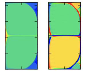
Axial wavenumber dependence of the Taylor vortex solutions. The parameters are $\eta =5/7$, $R_i=8\times 10^4$, $R_o=0$, which correspond to $Ta=9.75\times 10^9$ in figure 1. (a) The bifurcation diagram. The blue dotted curve is the Taylor vortex solution branch. This branch bifurcates from the linear critical point $L$ of the circular Couette flow. There is another linear critical point at very small $k$, but computing the bifurcating solution branch at this Taylor number is difficult, hence it is omitted. (b–d) Azimuthal velocity $v$ at the selected points in (a). The colour bar range is $[0,80\,000]$. All the solutions possess reflectional symmetry in $z$. (e, f) Enlarged views of parts of (c,d), respectively. The colour bar range is changed to $[10\,000,70\,000]$ in the enlarged figures.

In the ultimate turbulence, on the other hand, the situation appears to be more intricate. The snapshots of turbulence are typically accompanied by eddies of a vast scale, whereby the large-scale Taylor vortex is blurred in the time-averaged field. In particular, small turbulent eddies appearing in the boundary layer have been pointed out as a critical qualitative difference between the two turbulent regimes separated by the transition point seen in figure 1 (Dong Reference Dong2007; Ostilla-Mónico et al. Reference Ostilla-Mónico, van der Poel, Verzicco, Grossmann and Lohse2014a). Therefore, solutions with larger wavenumbers may play a more critical role in the turbulent dynamics. Our Nusselt number results also support this speculation. As seen in figure 1, the Taylor vortex with fixed $k$ underestimates experimental $Nu$ in the ultimate regime. However, if $k$ is optimised to maximise $Nu$ (the crosses in figure 1), then it can reach the experimental values for $Ta \lesssim 10^{11}$.

Figure 3(a) shows how $Nu$ changes as the wavenumber $k$ of the Taylor vortex is varied. The $Nu$ curve has two local maxima. The bimodal distribution of $Nu$ and the scaling of the two peaks are remarkably similar to those seen in the RBC roll cell computation by Waleffe et al. (Reference Waleffe, Boonkasame and Smith2015) and Sondak et al. (Reference Sondak, Smith and Waleffe2015). Based on their calculations at several Rayleigh numbers $Ra$, the first (second) peak has the wavenumber scaling $k\propto Ra^{0.217}$ ($Ra^{0.256}$) with the Nusselt number scaling exponent $\beta$ slightly larger (smaller) than 0.31. We will provide a theoretical rationale for the scaling in §§ 5 and 6.

For the ultimate turbulence regime, the approximation of the turbulent mean flow by the $k=3$ state is slightly worse (figure 2b). However, the mean flow of course varies with $k$. As the value of $k$ is increased from 3, the mean flow of the solution in the core region approaches a turbulent profile in the vicinity of the second peak. Figures 3(c) and 3(d) show the flow field at each peak, which is also examined in detail in the following two sections.

4. Taylor vortices with an $O(1)$ cell aspect ratio

In figure 2(a), we saw that some kind of homogenisation occurs in the core region of the Taylor vortex, and a thin boundary layer emerges around it. Such a flow structure looks very much like the high-Rayleigh-number RBC roll cell, which was studied intensively from the 1950s to the 1970s, for example, by Pillow (Reference Pillow1952), Robinson (Reference Robinson1967) and Wesseling (Reference Wesseling1969). More recently, it was reported that when the slip walls are imposed, the asymptotic solution can be calculated semi-analytically and is in good agreement with the numerical solutions (Chini & Cox Reference Chini and Cox2009; Hepworth Reference Hepworth2014). However, as noted by Robinson (Reference Robinson1967), for no-slip walls, the scaling and structure of the boundary layer have to be modified, which makes analytical progress difficult. The situation in the Taylor vortex is close to the latter problem, as we will see below.

First, let us examine the core region. For RBC, the roll cell vorticity in this region is known to become constant due to the Prandtl–Batchelor theorem, which states that the homogenisation of the vorticity occurs in the region where the streamlines are closed in two-dimensional inviscid flows (Prandtl Reference Prandtl1904; Batchelor Reference Batchelor1956; Feynman & Lagerstrom Reference Feynman and Lagerstrom1956). Moreover, the temperature becomes constant as well because the temperature equation has a structure similar to that of the vorticity equation (see e.g. Moore & Weiss Reference Moore and Weiss1973). To better see what precise physical quantities are homogenised in the core of the Taylor vortex, it is desirable to choose large gaps. Figure 4 shows the results for $\eta =0.5$. The colour map shown in figure 4(b) indicates clearly that it is actually angular momentum $rv$ that becomes uniform in the region where the streamlines are closed. Also, figure 4(c) shows that it is not the azimuthal vorticity $\omega$ that homogenises, but $\omega /r$.

Figure 4.

The flow field of the Taylor vortex for $\eta =0.5$, $k=3$. The Reynolds numbers used are $R_i=8\times 10^4$, $R_o=0.25 R_i$, corresponding to $Ta=1.40\times 10^{10}$, $a=-1/8$. (a) The Stokes streamfunction $\varPsi$. The colour bar range is $[-7500,7500]$. (b) The angular momentum $rv$. The colour bar range is $[40\,000,80\,000]$. (c) The modified azimuthal vorticity $\omega /r$. The colour bar range is $[-120\,000,120\,000]$. This quantity is distributed uniformly in the core to a value of approximately $\pm 37$ % of the colour bar.

Building on the above observations, now we introduce the new variables $\varGamma =Ta^{-1/2}\,rv$ and $\varOmega =\omega /r$, whereby the governing equations (2.6) are rewritten as

(4.1a)$$\begin{gather} \varPsi_r \varGamma_z - \varPsi_z \varGamma_r =(r^3(r^{{-}2}\varGamma)_r)_r+r\varGamma_{zz}, \end{gather}$$

(4.1b)$$\begin{gather}\varPsi_r \varOmega_z - \varPsi_z \varOmega_r = (r^{{-}1}(r^2\varOmega)_r)_r+{r\varOmega}_{zz} +Ta\,\frac{2\varGamma \varGamma_z}{r^3}, \end{gather}$$

(4.1c)$$\begin{gather}\varOmega={-}r^{{-}1}\{(r^{{-}1}\varPsi_r)_r+r^{{-}1}\varPsi_{zz} \}. \end{gather}$$

Here, the subscript $r$ or $z$ denotes a partial differentiation. The no-slip conditions become

(4.2a)$$\begin{gather} \varPsi=\varPsi_r=0, \quad \varGamma=\varGamma_i\equiv \frac{8\eta^3}{(1-\eta)(1+\eta)^3(1+ a)}\quad \text{at} \ r=r_i, \end{gather}$$

(4.2b)$$\begin{gather}\varPsi=\varPsi_r=0, \quad \varGamma=\varGamma_o\equiv{-}\frac{8\eta a}{(1-\eta)(1+\eta)^3 (1+ a)}\quad \text{at} \ r=r_o. \end{gather}$$

If $\varGamma$ is considered as temperature, $\varOmega$ as roll cell vorticity and $Ta$ as Rayleigh number, then one may notice that the structure of the equations is very similar to that of the two-dimensional RBC. The last term in the right-hand side of (4.1b) corresponds to the Coriolis force when the rotating plane Couette flow (RPCF) limit is taken, and it plays a role of buoyancy. (This term is not exactly the Coriolis force unless the system is in the RPCF limit, but for simplicity we will call it ‘Coriolis force’ hereafter; see Appendix A also.) This analogy in the sense of the structure of the equations would explain why $\varGamma$ and $\varOmega$ become constant in the Taylor vortex core, as seen in figure 4, at least on an intuitive level.

In fact, following Batchelor (Reference Batchelor1956), a mathematical argument can be developed. First, assuming that the typical roll cell circulation strength $Re_w$ (the wind Reynolds number) is asymptotically large, we expand $\varPsi =Re_w\,\varPsi _0+\cdots$, $\varGamma =\varGamma _0+\cdots$ and $\varOmega =Re_w\,\varOmega _0+\cdots$. Then the leading-order part of (4.1a) becomes $\varPsi _{0r} \varGamma _{0z}-\varPsi _{0z} \varGamma _{0r}=0$, which suggests that the function $\varGamma _0$ depends only on $\varPsi _0$. Now, in the $r$–$z$ plane, take a region $\mathcal {A}$ enclosed by a streamline $\mathcal {C}$ oriented counterclockwise (thus $\varPsi$ is constant along $\mathcal {C}$). Integrating (4.1a) over $\mathcal {A}$, we obtain

(4.3)\begin{equation} \int_{\mathcal{A}} \{\varPsi_r \varGamma_z - \varPsi_z \varGamma_r\} \,{\rm d}r\,{\rm d}z =\int_{\mathcal{A}} \{(r^3(r^{{-}2}\varGamma)_r)_r+(r^3(r^{{-}2}\varGamma)_z)_z\} \,{\rm d}r\,{\rm d}z.\end{equation}

The left-hand side vanishes because upon using the Stokes theorem it becomes

(4.4)\begin{equation} \int_{\mathcal{A}} \{(\varPsi_r \varGamma)_z - (\varPsi_z \varGamma)_r\} \,{\rm d}r\,{\rm d}z ={-}\oint_{\mathcal{C}} \varGamma \{\varPsi_z \boldsymbol{e}_z+\varPsi_r \boldsymbol{e}_r\} \boldsymbol{\cdot} {\rm d}\boldsymbol{l}=0. \end{equation}

The second equality comes from the fact that the gradient of $\varPsi$ and the line element on $\mathcal {C}$, ${\rm d}\boldsymbol {l}$, are orthogonal on the streamline. Meanwhile the leading-order part of the right-hand side can be transformed by again applying the Stokes theorem:

(4.5)\begin{align} 0&=\oint_{\mathcal{C}} r^3\{(r^{{-}2}\varGamma_0)_r\boldsymbol{e}_z-(r^{{-}2}\varGamma_0)_z\boldsymbol{e}_r\} \boldsymbol{\cdot} {\rm d}\boldsymbol{l} \nonumber\\ &=\frac{{\rm d}\varGamma_{0}}{{\rm d}\varPsi_0}\oint_{\mathcal{C}} r^2\{r^{{-}1}\varPsi_{0r}\boldsymbol{e}_z-r^{{-}1}\varPsi_{0z}\boldsymbol{e}_r\} \boldsymbol{\cdot} {\rm d}\boldsymbol{l} -2 \varGamma_0 \oint_{\mathcal{C}} \boldsymbol{e}_z \boldsymbol{\cdot} {\rm d}\boldsymbol{l} \nonumber\\ &=\frac{{\rm d}\varGamma_{0}}{{\rm d}\varPsi_0}\oint_{\mathcal{C}} r^2\{u_0\boldsymbol{e}_r+w_0\boldsymbol{e}_z\}\boldsymbol{\cdot} {\rm d}\boldsymbol{l}. \end{align}

Here, $(u_0, w_0)=(-r^{-1}\varPsi _{0z},r^{-1}\varPsi _{0r})$ is the leading-order part of the roll velocity. The integral in the last line should not vanish because we are assuming the existence of a strong circulation due to the swirling motion of the Taylor roll. Thus the equation implies ${{\rm d}\varGamma _{0}}/{{\rm d}\varPsi _0}=0$ at the value of $\varPsi _0$ on ${\mathcal {C}}$ that we choose. The above argument holds for any region enclosed by a streamline, hence the value of $\varGamma _0$ must be constant in the core region. The argument above does not change when an arbitrary constant is added to $\varGamma$. This implies that if power series asymptotic expansion of $\varGamma$ is considered, then the homogenisation also occurs in all the higher-order terms as long as they have a spatial scale of $O(1)$. Therefore, for steady solutions, the non-uniform component in $\varGamma$ is exponentially small.

Likewise, we can show that the value of $\varOmega _0$ is constant as well in the core. Integrating (4.1b) over ${\mathcal {A}}$ gives

(4.6)\begin{align} \int_\mathcal{A} \{\varPsi_r \varOmega_z - \varPsi_z \varOmega_r \} \,{\rm d}r\,{\rm d}z &=\int_\mathcal{A} \{(r^{{-}1}(r^2\varOmega)_r)_r+(r^{{-}1}(r^2\varOmega)_{z})_z\}\,{\rm d}r\,{\rm d}z \nonumber\\ &\quad +\int_\mathcal{A} Ta\,\frac{2\varGamma \varGamma_z}{r^3} \,{\rm d}r \,{\rm d}z, \end{align}

and of course the left-hand side should vanish. Since we already know that $\varGamma _0$ is a constant plus an exponentially small fluctuation, the last term in the right-hand side of (4.6) can be neglected. From (4.1b), we see that $\varOmega _0$ is a function of $\varPsi _0$, thus the leading-order part of integral (4.6),

(4.7)\begin{align} 0&=\oint_{\mathcal{C}} r^{{-}1}\{(r^2\varOmega_0)_r\boldsymbol{e}_z-(r^2\varOmega_0)_{z}\boldsymbol{e}_r)\}\boldsymbol{\cdot} {\rm d}\boldsymbol{l} \nonumber\\ &=\frac{{\rm d}\varOmega_{0}}{{\rm d}\varPsi_0} \oint_{\mathcal{C}} r^2\{r^{{-}1}\varPsi_{0r} \boldsymbol{e}_z-r^{{-}1}\varPsi_{0z}\boldsymbol{e}_r\}\boldsymbol{\cdot} {\rm d}\boldsymbol{l}+2\varOmega_0 \oint_{\mathcal{C}} \boldsymbol{e}_z \boldsymbol{\cdot} {\rm d}\boldsymbol{l} \nonumber\\ &=\frac{{\rm d}\varOmega_{0}}{{\rm d}\varPsi_0}\oint_{\mathcal{C}} r^2\{u_0\boldsymbol{e}_r+w_0\boldsymbol{e}_z\}\boldsymbol{\cdot} {\rm d}\boldsymbol{l}, \end{align}

yields ${{\rm d}\varOmega _{0}}/{{\rm d}\varPsi _0}=0$.

In the above argument, we have assumed that the swirling speed of the rolls is sufficiently large, but to see exactly how large it is, we need to analyse the boundary layer. Let us now take the region $\mathcal {A}$ as large as possible, and assume that a viscous boundary layer appears around its boundary $\mathcal {C}$. In this core region (see figure 5a), we have the estimation $Re_w=O(\varPsi |_c)= O(\varOmega |_c)$, where the subscript $c$ indicates that the physical quantities are measured in the core. At the roll cell perimeter $\mathcal {C}$, without loss of generality, we can set $\varPsi =0$. Hence if the thickness of the boundary layer is written as $\epsilon$, then the size of the streamfunction there can be estimated as $O(\varPsi |_b)= O(\epsilon \varPsi |_c)=O(\epsilon Re_w)$ (where the subscript $b$ stands for boundary layer). In order to ensure the viscous-convective balance of (4.1b) in this thin layer, we further require $O(\varPsi |_b)=O(\epsilon ^{-1})$, and therefore $Re_w=O(\epsilon ^{-2})$.

Figure 5.

Sketch of the asymptotic states. In the blue shaded region, viscosity is not negligible. In the dotted region, Coriolis force is at work. (a) Taylor vortex with aspect ratio of order unity ($k=O(1)$). (b,c) The first peak state ($k=O(Ta^{2/9})$), where (b) is the close-up of the near-wall zone enclosed by the red lines in (c).

As seen in figure 4(c), parts of the boundary layer are attached to the walls, where the flow has to fulfil the no-slip conditions. In order for the streamfunction to be modified in the near-wall boundary layer, both sides of (4.1c) must balance, so $O(\varOmega |_b)=O(\epsilon ^{-1}\,Re_w)$ using $\partial _r=O(\epsilon ^{-1})$ and $O(\varPsi |_b)=O(\epsilon ^{-1})$. Another essential part of the boundary layer is the plume, where the layer is detached from the wall. When the boundary layer leaves the wall, it typically forms a sharp corner. Similar to the RBC cases, as we round the corner, the sizes of $\varOmega$ and $\varGamma$ are unchanged. This can be justified by considering a streamline within the boundary layer. The streamline passes through the $O(\epsilon ^{1/2})$ neighbourhood of the corner, where the flow is inviscid, hence $\varOmega$ and $\varGamma$ are functions of the streamfunction; see also the RBC literature introduced at the beginning of this section.

The plume layer is no longer parallel to the wall, and the Coriolis force acting there drives the whole Taylor cell. This plume balance allows us to completely fix the flow scaling in terms of $Ta$. Assuming $\partial _r=O(1)$ and $\partial _z=O(\epsilon ^{-1})$ in (4.1b), the viscous-convective terms of $O(\epsilon ^{-2}\varOmega |_b)=O(\epsilon ^{-5})$ counterbalance the Coriolis term of $O( \epsilon ^{-1}\,Ta)$ when $\epsilon =Ta^{-1/4}$. Here, we used the fact that within the near-wall boundary layer, the size of $\varGamma$ is $O(1)$ from the boundary conditions, and the same size must be used in the plume.

The asymptotic structure can be summarised as follows. Within the core region, we use the expansions

(4.8a–c)\begin{equation} \varPsi=\epsilon^{{-}2}\omega_0\,\varPsi_0(r,z)+\cdots,\quad \varGamma=\gamma_0+\cdots,\quad \varOmega=\epsilon^{{-}2}\omega_0+\cdots,\end{equation}

where $\omega _0$ and $\gamma _0$ are constants. The expansion is consistent with the Prandtl–Batchelor structure to leading order, and $\varPsi _0$ must be determined by

(4.9)\begin{equation} 1={-}r^{{-}1}\{(r^{{-}1}\varPsi_{0r})_r+r^{{-}1}\varPsi_{0zz} \}\end{equation}

in the aforementioned region $\mathcal {A}$ with the boundary condition $\varPsi _0=0$ on $\mathcal {C}$.

Let $l$ and $n$ be the distance along $\mathcal {C}$ and its inward normal, respectively. Then using the rescaled normal variable $N=\epsilon ^{-1} n$, the flow within the boundary layer can be expanded as

(4.10a,b)\begin{equation} \varPsi=\epsilon^{{-}1}\,\varPsi^{(b)}(l,N)+\cdots,\quad \varGamma=\varGamma^{(b)}(l,N)+\cdots.\end{equation}

The leading-order equations in the boundary layer are

(4.11)$$\begin{gather} (\varPsi_{l}^{(b)}\,\partial_{N} - \varPsi_{N}^{(b)}\,\partial_{l})\varGamma^{(b)} =r\varGamma_{NN}^{(b)}, \end{gather}$$

(4.12)$$\begin{gather}(\varPsi_{l}^{(b)}\,\partial_{N} - \varPsi_{N}^{(b)}\,\partial_{l})\varPsi_{NN}^{(b)} ={r\varPsi}_{NNNN}^{(b)} - \frac{2\cos \varphi}{r}\,\varGamma^{(b)} \varGamma_{N}^{(b)}, \end{gather}$$

where $\varphi$ is the angle between the $z$-axis and the $n$-axis.

When the boundary layer is in contact with the cylinder wall, the following boundary conditions must be imposed at $N=0$:

(4.13)$$\begin{gather} \varPsi^{(b)}=\varPsi_{N}^{(b)}=0,\quad \varGamma^{(b)} =\varGamma_i\quad \text{at the inner cylinder,} \end{gather}$$

(4.14)$$\begin{gather}\varPsi^{(b)}=\varPsi_{N}^{(b)}=0,\quad \varGamma^{(b)} =\varGamma_o\quad \text{at the outer cylinder.} \end{gather}$$

For the near-wall boundary layer, $\cos \varphi =0$ so (4.12) is none other than Prandtl's boundary layer equation, while for large $N$, the flow must match the core solution. Let $U(l)$ be the value of $\varPsi _{0n}$ on $\mathcal {C}$, which can be found by the core flow problem (4.9). Then as $N\rightarrow \infty$, the boundary layer solution must satisfy

(4.15a,b)\begin{equation} \varPsi^{(b)}\rightarrow \omega_0\,U(l)\,N,\quad \varGamma^{(b)} \rightarrow \gamma_0.\end{equation}

When the boundary layer is detached from the wall, similar far-field conditions should be applied on both sides as $N\rightarrow \pm \infty$.

The theoretical boundary layer thickness $\epsilon =Ta^{-1/4}$ implies the Nusselt number scaling $Nu\propto Ta^{\beta }$ with $\beta =1/4$. We can check if this is consistent with the angular momentum transport. By averaging (4.1a) with respect to $z$ and further integrating radially from $r_i$ to $r$, the transport balance can be obtained as

(4.16)\begin{equation} -\overline{\varPsi_z \tilde{\varGamma}}=r^3(r^{{-}2}\bar{\varGamma})_r+\frac{16\eta r_i^2}{(1+\eta)^4}\,Nu.\end{equation}

Here we use an overline to denote the average with respect to $z$, and write $\varGamma =\bar {\varGamma }(r)+\tilde {\varGamma }(r,z)$. Let us consider this balance at a sufficient distance from both walls. In the core region, $\tilde {\varGamma }$ would be exponentially small because of the Prandtl–Batchelor theorem, so the transport is extremely inefficient. The plume region of thickness $O(\epsilon )$ is hence the main contributor to the left-hand side, which can be estimated as $O(\epsilon (\partial _z \varPsi |_b)\tilde {\varGamma } |_b)=O(\epsilon ^{-1})$ using the scaling $\tilde {\varGamma }|_b=O(1)$, $\varPsi |_b=O(\epsilon ^{-1})$. This term indeed balances with the second term on the right-hand side.

The asymptotic structure derived here is consistent with the behaviour of the numerical Taylor vortex solution. Figure 6 summarises the numerical results for $\eta =0.5$, $a=-1/8$. The red solid curve shows the scaling $Nu\propto Ta^{1/4}$, which can also be seen in the data presented in figure 1 ($\eta =5/7$, $a=0$). The green dashed and blue dotted curves are $Ta^{-1/2}rv$ and $Ta^{-1/2}\omega /r$ measured at the centre of the roll cell. According to the theory, they converge towards the constants $\gamma _0$ and $\omega _0$, respectively. The scaling of $\omega /r$ corresponds to the scaling of $u,w$ in the core, and hence the scaling of $Re_w$.

Figure 6.

The large-$Ta$ asymptotic convergence of the Taylor vortex for $\eta =0.5$, $k=3$, $a=-1/8$. The red solid curve is almost horizontal, implying that the $Nu \propto Ta^{1/4}$ scaling derived for $k=O(1)$ holds. The green dashed and blue dotted curves are computed by $v$ and $\omega$ measured at the centre of the cell $(r,z)=(r_i+0.5,{\rm \pi} /2k)$, respectively.

One may have noticed that the exponent $\beta =1/4$ of the Nusselt number differs from the exponent $\beta =1/3$ deduced in the asymptotic analysis of Chini & Cox (Reference Chini and Cox2009) and Hepworth (Reference Hepworth2014). This discrepancy is due not to the differences in the flow driving mechanism but to the boundary conditions at the walls. If the zero stress condition is imposed, then the linear extrapolation of the core streamfunction already satisfies the boundary condition to leading order. This means that the balance $O(\varOmega |_b)= O(\epsilon ^{-1}\,Re_w)$ that we assumed for the no-slip case is not necessary. For the slip wall case, the magnitude of the vorticity does not change in the core and the boundary layer, so the strong vortex layer seen in figure 4(c) does not appear. If we use the balance $O(\varOmega |_b)=O(\varOmega |_c)= O(\epsilon ^{-2})$ instead for the scaling argument of the plume, then we have $\epsilon =Ta^{-1/3}$, as expected.

For the slip wall RBC, further analytical progress has been made using the fact that the boundary layer equations become linear and the roll cells are rectangular (Chini & Cox Reference Chini and Cox2009; Hepworth Reference Hepworth2014). In our case, however, we have to rely on numerical calculations because the boundary layer equations are fully nonlinear. Moreover, the shape of the core region is non-trivial due to the small vortices appearing near the corners (see figure 4c). This means that the core and boundary layer equations (4.9), (4.11), (4.12) need to be solved iteratively by updating the core shapes and constants $\gamma _0$ and $\omega _0$. Such numerical calculations are too challenging and out of the scope of this paper. Differences in the structure of the boundary layer also affect the $Pr$ dependence of the asymptotic solution of RBC. For the slip wall case, asymptotic solutions for different $Pr$ can be obtained by rescaling the $Pr=1$ solution. However, this is possible because the boundary layer is linear, which is not true for the no-slip case.

Finally, we show that the above analysis provides some insights into the structure of the mean flow. As already seen in figure 4(b), the angular momentum $rv$ is almost constant in the core region. Therefore, the mean angular momentum $r\bar {v}$ is expected to become a constant away from the wall. This is indeed the case for the numerical Taylor vortex solution (figure 7a). In the studies of TCF turbulence, on the other hand, the mean angular velocity $q$ is usually plotted, and it is often noted that the profile is linear in the core. At first glance, this appears to be the case, for example, when looking at figure 2(a), but this is because the cylinder gap ($\eta \approx 0.714$) is too narrow to clearly see the radial dependence of the profile (see figure 7(a) for the $q$ profile for a wide gap case $\eta =0.5$). If the numerical results by Ostilla-Mónico et al. (Reference Ostilla-Mónico, van der Poel, Verzicco, Grossmann and Lohse2014b) are summarised in terms of $rv$, as shown in figure 7(b), then they clearly show the constant angular momentum property in the core. Note that when $a$ becomes too large, the Taylor vortex appears to favour the vicinity of the inner cylinder, and the homogenisation is observed only there. In the long history of TCF studies, some researchers have also pointed out that the turbulent mean flows might have a uniform angular momentum zone (Wattendorf Reference Wattendorf1935; Taylor Reference Taylor1935; Smith & Townsend Reference Smith and Townsend1982; Lewis & Swinney Reference Lewis and Swinney1999; Dong Reference Dong2007; Brauckmann & Eckhardt Reference Brauckmann and Eckhardt2017). However, this fact is not widely known, probably because the mathematical reasons behind it have not been elucidated.

Figure 7.

Uniform mean angular momentum profiles. (a) Mean flow of the Taylor vortex solution shown in figure 4 ($\eta =0.5$, $a=-1/8$). The red solid curve is the normalised angular momentum, while the blue dotted curve is the mean angular velocity $q$ defined in (3.1). (b) Time average of DNS results for $Ta=10^{10}$, ${a=-0.20},0.00,0.21,0.40,0.60,1.00$. The data are from figure 4 of Ostilla-Mónico et al. (Reference Ostilla-Mónico, van der Poel, Verzicco, Grossmann and Lohse2014b).

5. High-wavenumber Taylor vortices

The aim of this section is to examine the asymptotic behaviour of the solutions at the first and second peaks seen in figure 3(a). To this end, in figure 8, we performed similar calculations at two higher Taylor numbers. The results are summarised using the theoretical scaling to be derived in this section. Essentially, the scalings of $k$ and $Nu$ represent the width of the roll cell in the $z$ direction and the thickness of the boundary layer adjacent to the cylinder wall, respectively. The computations of the solutions are not easy, especially around the first peak, where very thin boundary layers need to be resolved. Although the convergence of the numerical solutions to the asymptotic states is still not perfect, the theoretical scalings are consistent with the overall features of the numerical data.

Figure 8.

Change in the Nusselt number of the Taylor vortex solution when the wavenumber is varied, with (a,b) using the same numerical results. The outer cylinder is stationary ($a=0$), and the radius ratio is ${\eta =5/7}$. Red solid, green dashed and blue dotted curves correspond to $Ta=2.95\times 10^{11}$, $Ta=7.37\times 10^{10}$ and $Ta=9.75\times 10^9$, respectively. The blue dotted curve is the same as that shown in figure 3. The three crosses in figure 1 are taken from the maxima seen in (a).

The structure of the flow field in both peaks can be divided roughly into a boundary layer near the wall and a core region in the middle of the gap, as we have seen in figures 2 and 3. On closer inspection, one further notices that the asymptotic structures of the two flows are quite different. For example, in the first peak solution, $\bar {\varGamma }$ has a flat profile in the core region (figure 9a), but this is not the case in the second peak solution (figure 9b). Figure 10 examines how the core flows develop from the near-wall region adjacent to the inner cylinder. In the first peak solution, the near-wall structure is somewhat similar to the $k=O(1)$ case, with the wall boundary layer becoming a sharp plume as rounding the corner (figure 10a). On the other hand, in the second peak solution, no apparent plume can be recognised away from the wall, and the flow varies only slowly in the $z$ direction (figure 10b). The core flow inherits this property, as seen from figure 11, where the axial structure of the fluctuation fields is plotted at the mid-gap $r=r_m=(r_o+r_i)/2$. For the second peak solution, only a single Fourier mode plays a major role in the core, while for the first peak, a number of harmonics participate in forming the plume. A theoretical explanation of those differences will be deduced below, together with the detailed scalings of the flows.

Figure 9.

Mean flows for the solutions at the extrema of $Nu$ seen in figure 8 ($\eta =5/7$, $a=0$). The red curves are the numerical results at $Ta=2.95\times 10^{11}$. (a) The first peak. The black solid line is the asymptotic result $\bar {\varGamma }=\gamma _0$. The value of $\gamma _0=0.771$ is estimated at the mid-gap. (b) The second peak. The black curve is the asymptotic result (6.5). The value $A=335.5$ is estimated at the mid-gap (see (6.39)).

Figure 10.

The colour map of $\omega /r$ for the (a) first peak and (b) second peak solutions seen in figure 8. Here, $Ta=2.95\times 10^{11}$. The centre of the colour bar is zero.

Figure 11.

The flow fields at the mid-gap $r=r_m$ for the (a,c) first peak and (b,d) second peak solutions in figure 8. The red solid, green dashed and blue dotted curves correspond to $Ta=2.95\times 10^{11}$, $Ta=7.37\times 10^{10}$ and $Ta=9.75\times 10^9$, respectively. Note that the value of $k$ is determined by the optimisation of $Nu$ and therefore varies from solution to solution. The difference in the structure of the first and second peak solutions can be seen more clearly in figure 10, where the axial coordinates are not scaled.

5.1. The first peak asymptotic structure

Now let us find the scaling of the first peak solution. Hereafter, $\delta =1/k$ denotes the length scale of the cell in the $z$ direction. The flow can be divided into core and near-wall zones, as shown in figure 5(c). Within the regions $O(\delta )$ away from the cylinder walls, similar asymptotic arguments as the $k=O(1)$ case would apply. Figure 5(b) shows an enlarged view of the near-wall zone where a thin boundary layer, of thickness $\epsilon \ll \delta$ say, emerges around the inviscid region.

The size of the streamfunction in the inviscid region must be the same as that of the core, $\varPsi |_c$. Thus the size of the streamfunction within the boundary layer can be found as $O(\varPsi |_b)=O(\epsilon \delta ^{-1} \varPsi |_c)$, noting that the boundary layer thickness relative to the near-wall region is $\epsilon /\delta$. Further using the viscous-convective balance in the boundary layer $O(\varPsi |_b)=O(\epsilon ^{-1}\delta )$, we can find $O(\varPsi |_c)=O(\delta ^{2}\epsilon ^{-2})$. When $\bar {\varGamma }|_c$ is almost constant, the viscous-convective balance in the core is satisfied if $O(\varPsi |_c)=O(\delta ^{-1})$. Hence from $O(\varPsi |_c)=O(\delta ^{2}\epsilon ^{-2})$ obtained in the near-wall analysis, the two small perturbation parameters are related as $\epsilon =\delta ^{3/2}$.

Within the near-wall zone, the plume coming out of the wall boundary layer is so thin that the Coriolis forces and viscous terms cannot balance, unlike the $k=O(1)$ case. This means that the Coriolis force effect should appear as the plume diffuses towards the core region.. The viscous-Coriolis balance in the core can be described as $O(\varPsi |_c\,\delta ^{-4})=O(Ta\, \delta ^{-1}\tilde {\varGamma }|_c)$. To estimate $O(\tilde {\varGamma }|_c)$, we can use the balance $O(\tilde {\varGamma } |_c\varPsi |_c)=O(\varGamma |_b\varPsi |_b)$, which will be justified shortly. Using the argument of the inviscid corner, we have $O(\varGamma |_b)=O(1)$. Therefore we have the estimation $O(\tilde {\varGamma }|_c)=O(\epsilon \delta ^{-1})$, which is consistent with the momentum transport balance $O((\partial _z \varPsi |_c)\tilde {\varGamma }|_c)=O(Nu)=O(\epsilon ^{-1})$, deduced from (4.16). This is the final key to unlock the scaling $\delta =O(Ta^{-2/9})$ and $\epsilon =O(Ta^{-1/3})$, with the latter motivating us to use the $Nu\propto Ta^{1/3}$ scaling in figure 8(a). The wind Reynolds number can be estimated by the wall-normal velocity component as $Re_w=O(\delta ^{-1}\varPsi |_c)=O(Ta^{4/9})$.

The asymptotic analysis in the core is summarised as follows. First, we choose $\delta$ as a small perturbation parameter and rescale the axial coordinate as $Z=\delta ^{-1} z$. From the scaling argument, the Taylor number has the expansion $Ta=\delta ^{-9/2}T_0+\cdots$. Using the core expansions

(5.1a,b)\begin{equation} \varPsi=\delta^{{-}1}\,\varPsi^{(c)}(r,Z)+\cdots,\quad \varGamma=\gamma_0+\delta^{1/2}\,\varGamma^{(c)}(r,Z)+\cdots \end{equation}

with a constant $\gamma _0$ in (4.1) yields the leading-order equations

(5.2)$$\begin{gather} (\varPsi_{r}^{(c)}\partial_Z-\varPsi_{Z}^{(c)}\partial_{r})\tilde{\varGamma}^{(c)}=r_i\tilde{\varGamma}_{ZZ}^{(c)}, \end{gather}$$

(5.3)$$\begin{gather}(\varPsi_{r}^{(c)}\partial_Z-\varPsi_{Z}^{(c)}\partial_{r})\varPsi_{ZZ}^{(c)}=r_i\varPsi_{ZZZZ}^{(c)}-T_0\,\frac{2\gamma_0}{r_i}\,\tilde{\varGamma}_{Z}^{(c)}. \end{gather}$$

Here, only the fluctuation part of the equations was extracted. The mean part can be obtained directly from (4.16) as

(5.4)\begin{equation} -\overline{\varPsi_{Z}^{(c)}\tilde{\varGamma}^{(c)}}=N_0, \end{equation}

using the scaled Nusselt number $N_0=({16\eta r_i^2}/{(1+\eta )^4})\epsilon \,Nu+\cdots$.

In the plume near the inner wall, we use the expansions

(5.5a,b)\begin{equation} \varPsi=\epsilon^{{-}1}\delta\,\varPsi^{(b)}(l,N)+\cdots,\quad \varGamma=\varGamma^{(b)}(l,N)+\cdots \end{equation}

together with the stretched variables $l=({r-r_i})/{\delta }$ and $N=z/\epsilon$. The leading-order part of (4.1a) takes the form

(5.6)\begin{equation} \varPsi_l^{(b)} \varGamma_N^{(b)}-\varPsi_N^{(b)} \varGamma_l^{(b)}= r_i \varGamma_{NN}^{(b)}, \end{equation}

which is essentially identical to (4.11). If we consider that $\varGamma ^{(b)}$ is a function of $\psi =\varPsi ^{(b)}$ and $l$, then the equation becomes

(5.7)\begin{equation} {- \varGamma}_l^{(b)}=r_i (\psi_z \varGamma_{\psi}^{(b)})_{\psi}, \end{equation}

where $\varGamma _{\psi }^{(b)}$ should be small when far enough away from the plume. By integrating this equation across the plume, we get

(5.8)\begin{equation} \frac{{\rm d}}{{\rm d}l}\left (\int^{\infty}_{-\infty} \varGamma^{(b)} \,{\rm d}\psi \right) = 0. \end{equation}

The term in the bracket is conserved during the plume diffusion so that the balance $O(\tilde {\varGamma } |_c\,\varPsi |_c)=O(\varGamma |_b\,\varPsi |_b)$ must be satisfied. The effect of the plume entering the core has to be described by boundary conditions for (5.2)–(5.3) at $r=r_i,r_o$. The conditions could be written using the Dirac delta function as done in Vynnycky & Masuda (Reference Vynnycky and Masuda2013).

We do not solve the asymptotic problem, but the theory well explains the behaviour of the Taylor vortex solution. For example, the numerical results shown in figures 11(a) and 11(c) are summarised using the theoretical core scalings $\varOmega |_c=O(\delta ^{-2}\varPsi |_c)=O(Ta^{2/3})$ and $\tilde {\varGamma }|_c=O(Ta^{-1/9})$. In figure 9(a), the thin black line is the asymptotic approximation $\bar {\varGamma }\approx \gamma _0$ with the estimate $\gamma _0=Ta^{-1/2}\,r_m\, \bar {v}(r_m)\approx 0.771$.

From the numerical data, the Nusselt number at the first peak seems to be approximated by $Nu=0.027\,Ta^{1/3}$. The asymptotic line intersects with the $k=3$ curve shown in figure 1 at $Ta\approx 6\times 10^7$, which is not a bad approximation of the transition point between the classical and ultimate turbulence regimes.

5.2. The second peak asymptotic structure

The asymptotic structure of the second peak solution is more complex because three layers appear in the vicinity of the walls (see figure 12a). We refer to them as the bottom, middle and top boundary layers, in order from the cylinder wall. Understanding their precise scaling requires a delicate matched asymptotic expansion analysis, which we will leave for the next section. Here we will look only at how the flow scaling is determined intuitively. The argument below contains one assumption that is not strictly fulfilled, but the resultant scaling is nonetheless correct if some minor logarithmic factor effects are omitted.

Figure 12.

Sketch similar to figure 5 but for the asymptotic states when $k=Ta^{1/4}$. (a) The second peak state. BL stands for boundary layer. (b) The transitional state. The shear layer occurs around the critical radius $r=r_c$.

The key assumption is ${{\rm d}\bar {\varGamma }}/{{\rm d}r}=O(1)$ in the core, which did not hold for the first peak case. If the governing equations (4.1a) and (4.1b) are linearised around the mean flow, then the balances $O(\delta ^{-1}\varPsi |_c)=O(\delta ^{-2}\tilde {\varGamma })$ and $O(\delta ^{-4}\varPsi |_c)=O(\delta ^{-1}Ta\, \tilde {\varGamma }|_c)$ must be satisfied. Those balances determine $\delta =O(Ta^{-1/4})$ and $O(\tilde {\varGamma }|_c)=O(\delta \varPsi |_c)$. Further using $O((\partial _z \varPsi |_c)\tilde {\varGamma }|_c)=O(Nu)=O(\epsilon ^{-1})$ deduced from the mean equation (4.16), the core flow scaling can be written as $O(\varPsi |_c)=O(\epsilon ^{-1/2})$, $O(\tilde {\varGamma }|_c)=O(\delta \epsilon ^{-1/2})$.

Within the bottom boundary layer, the viscous-convective balance $O(\varPsi |_b)=O(\epsilon ^{-1} \delta )$ must, of course, be satisfied (the subscript $b$ implies that $\varPsi$ is measured at the bottom boundary layer). If we further assume the viscous-Coriolis balance $O(\varPsi |_b)=O(Ta\,\epsilon ^{4} \delta ^{-1})$, then we obtain $\epsilon =\delta ^{6/5}=Ta^{-3/10}$, which gives $Nu\propto Ta^{3/10}$ in figure 8(b). It is this balance that is mostly met, but in fact, is a little broken. As mentioned earlier, the effect of this slight imbalance appears as a logarithmic factor in the scaling of $\epsilon$ in the matched asymptotic expansion. The introduction of the logarithmic factor has little influence when examining the scaling of numerical data, so it was ignored in figure 8(b). Furthermore, as shown in figures 11(b) and 11(d), the core scalings $O(\varOmega |_c)=O(\delta ^{-2}\varPsi |_c)=O(Ta^{13/20})$ and $\tilde {\varGamma }|_c=O(Ta^{-1/10})$ without the logarithmic factor well explain the numerical results. Note that the scaling result suggests $Re_w=O(\delta ^{-1}\varPsi |_c)=O(\delta ^{-1}\epsilon ^{-1/2})=O(Ta^{2/5})$.

In the middle boundary layer, the flow coming towards the wall turns back in the region of aspect ratio approximately unity, so its thickness should be $O(\delta )$.

The top boundary layer is necessary for the nonlinearity of the fluctuation component to disappear towards the core. Its thickness $\varDelta =O(\delta \epsilon ^{-1/2})=O(Ta^{-1/10})$ can be obtained by the viscous-convective balance $O(\varDelta ^{-1}\delta ^{-1}\varPsi |_t)=O(\delta ^{-2})$ and $O(\varPsi |_t)=O(\varPsi |_c)$, where $O(\varPsi |_t)$ is the size of the streamfunction in the top boundary layer. One of the ways to ascertain the presence of the top boundary layer in the visualised flow field is to look at the extreme values of $\varOmega$ (see figure 10(b)) or $\tilde {\varGamma }$. Figure 13(a) shows the scaled fluctuation $\tilde {\varGamma }$ at the plume position $z={\rm \pi} /k$. It can be seen that the minima approach the wall as the Taylor number increases. In figure 13(b), the distance between the wall and the minima is scaled by the theoretical top boundary layer thickness $\varDelta$. As expected, all the curves almost overlap around the minima.

Figure 13.

The profile of $\tilde {\varGamma }$ at the plume position $z={\rm \pi} /k$ for the Taylor vortex solution at the second peak, with $\eta =5/7$, $a=0$. The red solid, green dashed and blue dotted curves correspond to $Ta=2.95\times 10^{11}$, $Ta=7.37\times 10^{10}$ and $Ta=9.75\times 10^9$, respectively.

6. Matched asymptotic expansion when $k=O(Ta^{1/4})$

The goal of this section is to derive a matched asymptotic expansion consistent with the behaviour of the second peak solutions. This asymptotic state can be reached by decreasing the wavenumber from the linear critical point, as seen in figure 8(b). However, for $k/Ta^{1/4}$ ranging from approximately 0.6 to 0.8, the appropriate scaling of the Nusselt number is $O(Ta^0)$, which is different from that observed for the second peak state; see figure 14(a). We will study this transitional state in § 6.1, followed by the analysis of the second peak in § 6.2.

Figure 14.

(a) Close-up of figure 8(b) around the bifurcation point. The black solid curve is the asymptotic result (6.17), which has the property that $Nu=1$ at $k/Ta^{1/4}=K_1$, and that $Nu\rightarrow \infty$ as $k/Ta^{1/4}\rightarrow K_{\infty }$. (b) Mean flow profile at $k/Ta^{1/4}=0.65, 0.7$. The black solid curves are the asymptotic result (6.15). The bullets indicate $r=r_c$ given in (6.13). The red points are the numerical Taylor vortex result for $Ta=9.75\times 10^9$. (c) Colour maps of $\omega /r$ for the numerical Taylor vortex. The top and bottom maps correspond to $k/Ta^{1/4}=0.7$ and 0.65, respectively. Lines are marked at $r=r_c$.

The most important previous work throughout this section is due to Denier (Reference Denier1992), who applied the Hall & Lakin (Reference Hall and Lakin1988) type high-wavenumber asymptotic theory to TCF in the narrow gap limit. As briefly commented in that paper, the extension of the theory to wide-gap cases should be straightforward. In § 6.1, we derive an analytic expression for the Nusselt number and compare it with the numerical solution for the first time.

As the solution moves away from the linear critical point in the transitional state, the vortex grows from the vicinity of the inner cylinder (figure 14c). The asymptotic state corresponding to the second peak appears when the vortex fills the entire gap. A similar scenario was suggested in Denier (Reference Denier1992) using a matched asymptotic expansion, but the scaling obtained is unfortunately not consistent with the behaviour of the numerical solutions. The main reason for this is that the matching is not actually possible in the two-layer boundary layer structure assumed in Denier (Reference Denier1992). In § 6.2, we will resolve that difficulty by modifying the structure of the near-wall zone to three layers.

We choose $\delta =k^{-1}$ as a small perturbation parameter and introduce the scaled axial variable $Z=\delta ^{-1}z$. According to Hall (Reference Hall1982), the linear critical point of curved flow problems typically has the Taylor number expansion $Ta=\delta ^{-4} T_0+\cdots$. This is also true for TCF from the linear critical point to the second peak.

6.1. The transitional states around the linear critical point

For simplicity, we fix the outer cylinder (i.e. $a=\varGamma _o=0$) as in Denier (Reference Denier1992). The analysis of the general cases ($a\neq 0$) is relegated to Appendix B as it is somewhat complex. The asymptotic structure of the transitional state is depicted in figure 12(b). The vortices are concentrated in the core region $r_i< r< r_c$, where $r_c \in [r_i,r_o]$ is the critical radius to be determined analytically. We can show that the vortex amplitude decays exponentially within a shear layer of thickness $O(\varDelta )=O(Ta^{-1/6})$ appearing around the critical radius. The structure of the shear layer is identical to that described in Denier (Reference Denier1992) and is not discussed in detail here. The only important fact that will be used later is that the mean flow and its derivative are continuous across this layer.

In the region where $r$ is greater than $r_c$, it is sufficient to analyse the mean flow. To leading order, the left-hand side of (4.16) can be ignored, hence the mean flow is a linear combination of a constant and $r^2$. Writing

(6.1)\begin{equation} N_0=\frac{16\eta r_i^2}{(1+\eta)^4}\,Nu\end{equation}

for simplicity, we get the asymptotic approximation

(6.2a,b)\begin{equation} \bar{\varGamma}=B(r_o^2-r^2)+\cdots,\quad B=\frac{N_0}{2r_o^2}.\end{equation}

Note that we used the fact that $\bar {\varGamma }$ should vanish at $r=r_o$.

In the core region, the appropriate expansions are

(6.3a–c)\begin{equation} \varPsi=\hat{\varPsi}^{(c)}(r)\sin Z+\cdots,\quad \tilde{\varGamma}=\delta\,\hat{\varGamma}^{(c)}(r)\cos Z+\cdots,\quad \bar{\varGamma}=\bar{\varGamma}^{(c)}(r)+\cdots. \end{equation}

Substituting these into (4.1), the leading-order parts yield

(6.4a,b)\begin{equation} \bar{\varGamma}_r^{(c)} \hat{\varPsi}^{(c)} =r\hat{\varGamma}^{(c)}, \quad 0=\hat{\varPsi}^{(c)}+T_0\,\frac{2\bar{\varGamma}^{(c)}}{r^2}\,\hat{\varGamma}^{(c)}.\end{equation}

For those equations to have a non-trivial solution, $0=r^3+2T_0\bar {\varGamma }^{(c)}\bar {\varGamma }^{(c)}_r$ must be satisfied. Therefore the mean flow is obtained as

(6.5)\begin{equation} \bar{\varGamma}^{(c)}(r)=\sqrt{\frac{A-r^4}{4T_0}}.\end{equation}

The constant $A$ must be

(6.6)\begin{equation} A=r_i^4+4T_0\varGamma_i^2\end{equation}

to satisfy $\bar {\varGamma }^{(c)}(r_i)=\varGamma _i$.

A boundary layer of thickness $O(\delta )$ is needed near the inner cylinder to satisfy the no-slip boundary conditions. In this layer, we introduce the stretched variable $\xi =({r-r_i})/{\delta }$ and assume the expansion

(6.7a,b)\begin{equation} \varPsi=\varPsi^{(b)}(\xi,Z)+\cdots,\quad \varGamma= \varGamma_i+\delta\,\varGamma^{(b)}(\xi,Z)+\cdots. \end{equation}

The leading-order equations are obtained as

(6.8)$$\begin{gather} (\varPsi_{\xi}^{(b)}\partial_Z-\varPsi_{Z}^{(b)}\partial_{\xi})\varGamma^{(b)}=r_i(\partial_{\xi}^2+\partial_Z^2)\varGamma^{(b)}, \end{gather}$$

(6.9)$$\begin{gather}(\varPsi_{\xi}^{(b)}\partial_Z-\varPsi_{Z}^{(b)}\partial_{\xi})(\partial_{\xi}^2+\partial_Z^2)\varPsi^{(b)}=r_i(\partial_{\xi}^2+\partial_Z^2)^2\varPsi^{(b)}-T_0\,\frac{2\varGamma_i\varGamma_{Z}^{(b)}}{r_i}. \end{gather}$$

The no-slip boundary conditions are

(6.10)\begin{equation} \varPsi^{(b)}=\varPsi_{\xi}^{(b)}=0,\quad \varGamma^{(b)}=0\quad \text{at} \ \xi=0, \end{equation}

while for the far field, $\xi \rightarrow \infty$, we use the matching conditions

(6.11a–c)\begin{equation} \varPsi^{(b)}\rightarrow \hat{\varPsi}^{(c)}(r_i)\sin Z,\quad \tilde{\varGamma}^{(b)} \rightarrow \hat{\varGamma}^{(c)}(r_i)\cos Z,\quad \bar{\varGamma}^{(b)}\rightarrow \bar{\varGamma}^{(c)}_r(r_i)\,\xi. \end{equation}

Finally, we determine the unknown constants $B$ and $r_c$ from the continuity of $\bar {\varGamma }$ and $r^3(r^{-2}\bar {\varGamma })_r$ at $r=r_c$. Using the mean flows (6.5) and (6.2a), the continuity conditions can be written as

(6.12a,b)\begin{equation} \sqrt{\frac{A-r_c^4}{4T_0}}=B(r_o^2-r_c^2),\quad \frac{A}{\sqrt{T_0(A-r_c^4)}}=2Br_o^2, \end{equation}

where $A$ is known by (6.6). From those equations, it is easy to find

(6.13)$$\begin{gather} r_c=\sqrt{\frac{r_i^4+4T_0\varGamma_i^2}{r_o^2}}, \end{gather}$$

(6.14)$$\begin{gather}\frac{1}{B}=\sqrt{4T_0\left (\frac{r_o^4}{r_i^4+4T_0\varGamma_i^2}-1 \right )}. \end{gather}$$

Thus if $T_0$ is given, then the leading-order mean flow is completely determined as

(6.15)\begin{equation} \bar{\varGamma}\approx \left \{\begin{array}{@{}ll@{}} (r_o^2-r^2)\sqrt{\dfrac{r_i^4+4T_0\varGamma_i^2}{4T_0\left (r_o^4-r_i^4-4T_0\varGamma_i^2 \right )}} & \text{if} \ r> r_c,\\[14pt] \sqrt{\dfrac{r_i^4-r^4+4T_0\varGamma_i^2}{4T_0}} & \text{if} \ r\leq r_c. \end{array} \right . \end{equation}

This is the black curve in figure 14(b), which predicts the numerical results very well. Note that the analytic expression for $\hat {\varPsi }^{(c)}$ and $\hat {\varGamma }^{(c)}$ can also be found by (6.4a,b) and the leading-order part of the mean flow equation (4.16):

(6.16)\begin{equation} -\frac{\bar{\varGamma}^{(c)}_r}{2r}\,(\hat{\varPsi}^{(c)})^2=r^3(r^{{-}2}\bar{\varGamma}^{(c)})_r+N_0. \end{equation}

The Nusselt number is found using (6.1), (6.2b) and (6.14) as

(6.17)\begin{equation} Nu(T_0)=\frac{(1+\eta)^4}{16\eta^3\sqrt{T_0}}\sqrt{\frac{r_i^4+4T_0\varGamma_i^2}{r_o^4-r_i^4-4T_0\varGamma_i^2}}.\end{equation}

This function is plotted by the black curve in figure 14(a), using $k/Ta^{1/4}= T_0^{-1/4}$ for the horizontal axis. The other curves, corresponding to the Taylor vortex solutions at finite $Ta$, clearly approach the asymptotic result as $Ta\rightarrow \infty$.

As the scaled wavenumber decreases from the linear critical point $K_1=T_1^{-1/4}$, the Nusselt number increases from the laminar value unity. The asymptotic result $T_1={r_i^2(r_o^2-r_i^2)}/{4\varGamma _i^2}$ can be found from (6.13) by setting $r_c=r_i$ and $T_0=T_1$.

Similar to the narrow gap case studied by Denier (Reference Denier1992), $Nu$ blows up at finite $T_0$. Writing $K_{\infty }=T_{\infty }^{-1/4}$, we can deduce $T_{\infty }=({r_o^4-r_i^4})/{4\varGamma _i^2}$ from (6.13) by using $r_c=r_o$ and $T_0=T_{\infty }$. That is, in figure 14(a), $K_{\infty }$ is the point at which the flow switches from the transitional state to the second peak state.

6.2. The second peak states

We now turn our attention to the second peak asymptotic states. Again, $\delta$ is the small asymptotic parameter, and $Ta=\delta ^{-4}T_0+\cdots$. For the bottom boundary layer thickness $\epsilon$, we impose the condition

(6.18)\begin{equation} \frac{\delta^6}{\epsilon^{5}}=\ln\frac{\delta}{\epsilon},\end{equation}

which is needed for successful matching. The boundary layer thickness is estimated as $O(\epsilon )=O(Ta^{-3/10}(\ln Ta)^{-1/5})$. Therefore the Nusselt number and the wind Reynolds number scalings now involve the logarithmic correction as $Nu=O(\epsilon ^{-1})=O(Ta^{3/10}(\ln Ta)^{1/5})$, $Re_w=O(\delta ^{-1}\varPsi |_c)=O(\delta ^{-1}\epsilon ^{-1/2})=O(Ta^{2/5}(\ln Ta)^{1/10})$.

Let us start with the core analysis by writing

(6.19)$$\begin{gather} \varPsi=\epsilon^{{-}1/2}\,\hat{\varPsi}^{(c)}(r)\sin Z+\cdots\,, \end{gather}$$

(6.20a,b)$$\begin{gather}\tilde{\varGamma}=\delta \epsilon^{{-}1/2}\,\hat{\varGamma}^{(c)}(r)\cos Z+\cdots,\quad \bar{\varGamma}=\bar{\varGamma}^{(c)}(r)+\cdots. \end{gather}$$

Those expansions, based on the argument in § 5, yield leading-order equations (6.4a,b) identical to those for the transitional state. As a result, the mean flow is given by (6.5). However, for the second peak state, the multi-layered near-wall structure must also be present near the outer cylinder, thus there is no way to determine the constant $A$ a priori. The leading-order part of the mean flow equation (4.16) is obtained as

(6.21)\begin{equation} -\frac{\bar{\varGamma}^{(c)}_r}{2r}\,(\hat{\varPsi}^{(c)})^2=N_0, \end{equation}

where $N_0=({16\eta r_i^2}/{(1+\eta )^4})\epsilon \,Nu$. The unknowns appearing in the core solutions $\bar {\varGamma }^{(c)}, \hat {\varPsi }^{(c)}$ and $\hat {\varGamma }^{(c)}$ are $A$ and $N_0$.

The two near-wall regions have identical asymptotic structure, so only the layers near the inner cylinder are examined below. The top boundary layer expansions are

(6.22a,b)\begin{equation} \varPsi=\epsilon^{{-}1/2}\,\varPsi^{(t)}(\zeta,Z)+\cdots,\quad \varGamma=\gamma_i+\delta \epsilon^{{-}1/2}\,\varGamma^{(t)}(\zeta,Z)+\cdots, \end{equation}

where the constant $\gamma _i=\bar {\varGamma }^{(c)}(r_i)$ comes from the leading-order core mean flow. The stretched variable $\zeta =({r-r_i})/{\varDelta }$ is defined by using the top boundary layer thickness $\varDelta =\delta \epsilon ^{-1/2}=O(Ta^{-1/10}(\ln Ta)^{1/10})$. The leading-order governing equations for the top boundary layer are similar to those for the core region in the first peak states:

(6.23)$$\begin{gather} (\varPsi_{\zeta}^{(t)}\partial_Z-\varPsi_{Z}^{(t)}\partial_{\zeta})\tilde{\varGamma}_t=r_i\tilde{\varGamma}_{ZZ}^{(t)}, \end{gather}$$

(6.24)$$\begin{gather}(\varPsi_{\zeta}^{(t)}\partial_Z-\varPsi_{Z}^{(t)}\partial_{\zeta})\varPsi_{ZZ}^{(t)}=r_i\varPsi_{ZZZZ}^{(t)}-T_0\,\frac{2\gamma_i}{r_i}\,\tilde{\varGamma}_{Z}^{(t)}, \end{gather}$$

(6.25)$$\begin{gather}-\overline{\varPsi_{Z}^{(t)}\tilde{\varGamma}^{(t)}}=N_0. \end{gather}$$

As $\zeta \rightarrow \infty$, the flow matches to the core solution as

(6.26a–c)\begin{equation} \varPsi^{(t)}\rightarrow \hat{\varPsi}^{(c)}(r_i)\sin Z,\quad \tilde{\varGamma}^{(t)} \rightarrow \hat{\varGamma}^{(c)}(r_i)\cos Z,\quad \bar{\varGamma}^{(t)}\rightarrow \bar{\varGamma}^{(c)}_r(r_i)\,\zeta, \end{equation}

while the asymptotic behaviour of the flow towards the wall should be

(6.27)\begin{equation} \varPsi^{(t)}\rightarrow \zeta^{1/3}\,\hat{\varPsi}^{(t)}(Z),\quad \varGamma^{(t)} \rightarrow \zeta^{{-}1/3}\,\hat{\varGamma}^{(t)}(Z)\quad \text{as}\ \zeta \rightarrow 0, \end{equation}

which is similar to that used in Denier (Reference Denier1992). However, to match this with the bottom boundary layer, we must insert the middle boundary layer.

Recall that the middle boundary layer is the special place where the radial and axial derivatives of the flow have the same size. Thus the expansions there must be written in terms of $\xi =({r-r_i})/{\delta }$ as

(6.28a,b)\begin{equation} \varPsi=\epsilon^{{-}1/3}\,\varPsi^{(m)}(\xi,Z)+\cdots,\quad \varGamma=\gamma_i+\delta \epsilon^{{-}2/3}\,\varGamma^{(m)}(\xi,Z)+\cdots. \end{equation}

Given the expansions, it is a straightforward task to find that the leading-order equations

(6.29)$$\begin{gather} (\varPsi_{\xi}^{(m)}\partial_Z-\varPsi_{Z}^{(m)}\partial_{\xi})\tilde{\varGamma}^{(m)}=0, \end{gather}$$

(6.30)$$\begin{gather}(\varPsi_{\xi}^{(m)}\partial_Z-\varPsi_{Z}^{(m)}\partial_{\xi})(\partial_{\xi}^2+\partial_Z^2)\varPsi^{(m)}={-}T_0\,\frac{2\gamma_i}{r_i}\,\tilde{\varGamma}_{Z}^{(m)}, \end{gather}$$

(6.31)$$\begin{gather}-\overline{\varPsi_{Z}^{(m)}\tilde{\varGamma}^{(m)}}=N_0, \end{gather}$$

are inviscid. Here, the Coriolis force term participating in (6.30) is critical for successful matching to the top boundary layer:

(6.32)\begin{equation} \varPsi^{(m)}\rightarrow \xi^{1/3}\,\hat{\varPsi}^{(t)}(Z),\quad \varGamma^{(m)} \rightarrow \xi^{{-}1/3}\,\hat{\varGamma}^{(t)}(Z)\quad \text{as}\ \xi\rightarrow \infty. \end{equation}

On the other hand, the appropriate behaviour of the solution towards the wall, $\xi \rightarrow 0$, can be found as

(6.33a,b)\begin{equation} \varPsi^{(m)}\rightarrow \xi (-\ln \xi)^{1/3}\,\hat{\varPsi}^{(b)}(Z),\quad \varGamma^{(m)} \rightarrow \xi^{{-}1}(-\ln \xi)^{{-}1/3}\,\hat{\varGamma}^{(b)}(Z) \end{equation}

by seeking the consistent limiting behaviour of the solution. The key observation here is that for both matching conditions, the rate of increase in $\varPsi$ and the rate of decrease in $\varGamma$ are the same when moving away from the wall. This is a requirement to satisfy the angular momentum transport balance (6.31).

The leading-order part of the bottom boundary layer expansions

(6.34a,b)\begin{equation} \varPsi=\frac{\delta}{\epsilon}\,\varPsi^{(b)}(Y,Z)+\cdots,\quad \varGamma= \varGamma^{(b)}(Y,Z)+\cdots \end{equation}

matches the middle boundary layer if (6.18) holds and

(6.35a,b)\begin{equation} \varPsi^{(b)}\rightarrow Y\,\hat{\varPsi}^{(b)}(Z),\quad \varGamma^{(b)} \rightarrow Y^{{-}1}\,\hat{\varGamma}^{(b)}(Z) \end{equation}

as $Y=({r-r_i})/{\epsilon } \rightarrow \infty$. The leading-order equations in the bottom boundary layer are

(6.36)$$\begin{gather} (\varPsi_{Y}^{(b)}\partial_Z-\varPsi_{Z}^{(b)}\partial_{Y})\varGamma^{(b)}=r_i\varGamma_{YY}^{(b)}, \end{gather}$$

(6.37)$$\begin{gather}(\varPsi_{Y}^{(b)}\partial_Z-\varPsi_{Z}^{(b)}\partial_{Y})\varPsi_{YY}^{(b)}=r_i\varPsi_{YYYY}^{(b)}. \end{gather}$$

Thanks to the radial diffusivity, the no-slip boundary conditions

(6.38)\begin{equation} \varPsi^{(b)}=\varPsi_{Y}^{(b)}=0,\quad \varGamma^{(b)}=\varGamma_i \quad \text{at} \ Y=0 \end{equation}

can be imposed.

Although the combined boundary layers appear rather complex, their role is merely to define the relationship between $A$ and $N_0$. Once $T_0$ and $A$ are fixed, the flow near the inner cylinder can be calculated to find $N_0=f_i(A,T_0)$. A similar calculation for the near outer cylinder region yields another functional relationship $N_0=f_o(A,T_0)$. Hence, in principle, $A(T_0)$ and $N_0(T_0)$ can be determined by solving the two near-wall regions numerically. We do not perform such challenging calculations since we have already seen in § 5 that the finite $Ta$ numerical results are consistent with the asymptotic theory.

The value of $A$ can be predicted from the finite $Ta$ numerical solutions as

(6.39)\begin{equation} A=(2k^{{-}2}r_m\,\bar{v}(r_m))^2+r_m^4\end{equation}

by using the mean flow at the mid-gap. The black curve in figure 9(b) is the result of using this $A$ in (6.5), and it can be seen that this asymptotic prediction matches the numerical calculation in the entire core region. Similarly, the fluctuation component in the core can be calculated explicitly. The black curve in figure 15 is the asymptotic approximation

(6.40)\begin{equation} \tilde{\varGamma}\approx Ta^{{-}1/4}\,r\left (\frac{32\eta r_i^2}{(1+\eta)^4}\,\frac{Nu}{\sqrt{(A-r^4)}} \right )^{1/2} \cos Z,\end{equation}

which is in good agreement with the numerical result.

Figure 15.

The red dotted curve is the profile of $\tilde {\varGamma }$ at the plume position $z={\rm \pi} /k$ for the Taylor vortex solution at the second peak. We use the same data as in figure 13 ($\eta =5/7$, $a=0$, $Ta=2.95\times 10^{11}$). The black curve is the asymptotic result (6.40).

We will also comment briefly on the case where $a$ is non-zero. For any $a$, it is not so difficult to decrease $k$ of the Taylor vortex solution branch from the linear critical point until the Nusselt number takes a peak. The red crosses in figure 16(a) summarise $Nu$ at the peak for various $a$. The numerical result shows that the optimised $Nu$ is maximised when the outer cylinder slightly counter-rotates ($a\approx 0.08$). This is in line qualitatively with the experimental ultimate turbulence results shown by green squares. However, for the experimental results, the maximum of $Nu$ is attained at $a\approx 0.3$ and, as noted in § 3, the Nusselt number scaling is $Nu\propto Ta^{0.38}$. The Taylor vortex results naturally have a much smaller $Nu$, because it is scaled like $Ta^{0.3}$ as the second peak seen in the $a=0$ case. In figure 16(b), we also plotted $K_1$ and $K_{\infty }$ obtained in the transitional state analysis (see (B5a,b) and (B7a,b) in Appendix B). Roughly speaking, the peaks occur when $k/Ta^{1/4}$ is approximately half of $K_{\infty }$. The linear and nonlinear instabilities disappear at the Rayleigh line $a=-\eta ^2\approx -0.51$, which can be found from Rayleigh's stability condition.

Figure 16.

(a) The Nusselt number at $Ta=10^{10}$ for $\eta =5/7$. The red crosses are the Taylor vortex solution with the optimised wavenumbers shown in (b). The green squares are experimental results by Dennis et al. (Reference Dennis, Huisman, Bruggert, Sun and Lohse2011). (b) The red crosses are the local maximum of $Nu$ closest to the bifurcation point. According to the asymptotic theory, the Taylor vortex solution bifurcates from circular Couette flow at $K_1$ (see (B5a,b)). The Nusselt number $Nu$ is $O(1)$ when $k/Ta^{1/4}\in (K_\infty, K_1)$, where $K_{\infty }$ is given in (B7a,b). For $k/Ta^{1/4}< K_\infty$, the $Nu$ scaling is like the second peak state.

Brauckmann, Salewski & Eckhardt (Reference Brauckmann, Salewski and Eckhardt2016) and Brauckmann & Eckhardt (Reference Brauckmann and Eckhardt2017) reported that when the gap is narrow, there are two values of $R_{\varOmega }=(1-\eta )({R_i+R_o})/({R_i-\eta R_o})$ at which the local maximum of $Nu$ occurs. Whether similar results can be obtained with the Taylor vortex solution is left for future work.