


1 Introduction
The language of turbulence is traditionally dichotomous. On the one hand there are scales and wavelengths and the notion of forward or reverse cascades of energy which are best suited to dealing with homogenous conditions, see Monin & Yaglom (Reference Monin and Yaglom1971a
). On the other hand, transport processes are described in physical space where inhomogeneity, Reynolds stresses and local turbulent kinetic energy production are the keywords, see Monin & Yaglom (Reference Monin and Yaglom1971b
). Contrary to quantum mechanics, where the complementarity is intrinsic to the microscopic world, in turbulence this duality is substantially an artefact induced by the formal tools used to study the problem. This is clearly seen by considering the well-known example of canonical wall bounded flows where the two aspects coexists. The equilibrium (logarithmic) layer is ideally traversed by a constant wall-normal flux of turbulent kinetic energy that sustains the fluctuations in the bulk. At the same time, the local production
 $u_{\unicode[STIX]{x1D70F}}^{3}/(\unicode[STIX]{x1D705}y)$
is confined to a range of scales limited below by the characteristic length
$u_{\unicode[STIX]{x1D70F}}^{3}/(\unicode[STIX]{x1D705}y)$
is confined to a range of scales limited below by the characteristic length
 $L_{shear}=\unicode[STIX]{x1D705}y$
, see Corrsin (Reference Corrsin1958), with energy cascading to small scale towards local dissipation, where
$L_{shear}=\unicode[STIX]{x1D705}y$
, see Corrsin (Reference Corrsin1958), with energy cascading to small scale towards local dissipation, where
 $\unicode[STIX]{x1D705}$
is the Kármán constant,
$\unicode[STIX]{x1D705}$
is the Kármán constant,
 $y$
is the distance from the wall and
$y$
is the distance from the wall and
 $u_{\unicode[STIX]{x1D70F}}=\sqrt{\unicode[STIX]{x1D70F}_{w}/\unicode[STIX]{x1D70C}}$
is the friction velocity, with
$u_{\unicode[STIX]{x1D70F}}=\sqrt{\unicode[STIX]{x1D70F}_{w}/\unicode[STIX]{x1D70C}}$
is the friction velocity, with
 $\unicode[STIX]{x1D70F}_{w}$
the average wall shear stress and
$\unicode[STIX]{x1D70F}_{w}$
the average wall shear stress and
 $\unicode[STIX]{x1D70C}$
the fluid density, see Townsend (Reference Townsend1980).
$\unicode[STIX]{x1D70C}$
the fluid density, see Townsend (Reference Townsend1980).
Overcoming the scale/position duality is particularly important for strongly non-equilibrium conditions, as in the buffer layer of the example above where the wall-normal flux originates, or in high Reynolds number flows around bluff bodies or behind abrupt section variations in channels or pipes. In the latter cases, recirculating regions form behind the obstacle, separated by intense shear layers from the external flow with open streamlines, see e.g. Landau & Lifshitz (Reference Landau and Lifshitz1987). Such flows are strongly inhomogeneous, with pronounced peaks of turbulent kinetic energy production. The local dissipation is insufficient to balance production and spatial fluxes move the energy downstream of the obstacle and into the recirculating bubble, see Mollicone et al. (Reference Mollicone, Battista, Gualtieri and Casciola2017) for a recent direct numerical simulation (DNS). Several questions naturally come to mind: What are the scales involved in these processes? How is the turbulent activity in the different ranges of scale distributed in space? Which mechanisms sustain eddies of different scale? For obvious reasons, single-point statistics cannot address these fundamental questions, but at the same time, the complementary balance in spectral space, Kolmogorov–Onsager–Heisenberg–von Weiszäcker–Lin equation, see e.g. Eyink & Sreenivasan (Reference Eyink and Sreenivasan2006), does not uncover the energy transfer in space, due to projection on non-local Fourier modes.
de Karman & Howarth (Reference de Karman and Howarth1938) and Kolmogorov (Reference Kolmogorov1941) originally devised their description of turbulence in terms of two-point observables (correlations and structure functions, respectively), see e.g. Frisch (Reference Frisch1995) for a comprehensive introduction, as a scale-by-scale approach to develop their theory of homogeneous and isotropic turbulence. Only recently, their theory has been progressively extended to more complex flows by using a generalised form of the Kolmogorov equation. The generalised Kolmogorov equation (GKE), see Hill (Reference Hill2002) for the derivation of the complete equation, accounts for anisotropic and inhomogeneous conditions and has been used in various studies of free shear by Casciola et al. (Reference Casciola, Gualtieri, Benzi and Piva2003, Reference Casciola, Gualtieri, Jacob and Piva2005), wall-bounded flows by Danaila et al. (Reference Danaila, Anselmet, Zhou and Antonia2001), Danaila, Anselmet & Zhou (Reference Danaila, Anselmet and Zhou2004), Marati, Casciola & Piva (Reference Marati, Casciola and Piva2004), Cimarelli, Angelis & Casciola (Reference Cimarelli, Angelis and Casciola2013) and wake turbulence by Gomes-Fernandes, Ganapathisubramani & Vassilicos (Reference Gomes-Fernandes, Ganapathisubramani and Vassilicos2015). Alternatively to GKE, other approaches are available to study the energy behaviour across the scales, see e.g. Cardesa, Vela-Martín & Jiménez (Reference Cardesa, Vela-Martín and Jiménez2017). Casciola et al. (Reference Casciola, Gualtieri, Benzi and Piva2003) address the link between the intermittency and anisotropy in homogeneous shear flows and employ the GKE to distinguish the shear-dominated scales by the small isotropic scales dominated by dissipation. Numerical data show that the dissipation scales are independent of the mean shear, thus intermittency corrections are universal. Danaila et al. (Reference Danaila, Anselmet, Zhou and Antonia2001) provide a generalised form of the Kolmogorov equation adding additional terms to account for the ‘large-scale turbulent diffusion acting from the walls through to the centreline of the channel’. The scale-by-scale budget in a planar turbulent channel flow is numerically studied by means of the GKE by Marati et al. (Reference Marati, Casciola and Piva2004) and Cimarelli et al. (Reference Cimarelli, Angelis and Casciola2013). Such understanding is fundamental to tune innovative techniques to control boundary layer transition to turbulence and to design innovative turbulence models, see Thiesset et al. (Reference Thiesset, Antonia, Danaila and Djenidi2013), since it is able to capture the correct dynamics of the fluctuations for inhomogeneous flows. Danaila et al. (Reference Danaila, Anselmet and Zhou2004) show the effects of turbulent diffusion and shear on the scale-by-scale budget far from the wall in a turbulent channel. The generalised equation is in agreement with hot-wire measurements in such regions, considered to be nearly sheared homogeneous turbulence. A more recent study by Cimarelli et al. (Reference Cimarelli, De Angelis, Schlatter, Brethouwer, Talamelli and Casciola2015), still concerning turbulent channel flow, focuses on peaks of scale energy found in both the near-wall region and overlap layer and the interaction between them. Gomes-Fernandes et al. (Reference Gomes-Fernandes, Ganapathisubramani and Vassilicos2015) address the energy transfer across the scales in a highly non-homogeneous, anisotropic turbulent flow generated by a fractal grid. They show that the inter-scale energy transfers are characterised by the combination of both inverse cascade in the streamwise direction and forward cascade in the spanwise direction, whilst the overall cascade is forward.
The aim of the present work is to understand the production and transfer of turbulent kinetic energy (TKE) in the combined space of positions and scales for a definitely more complex geometry. We introduce a bulge (also referred to as bump) at one of the walls in a periodic turbulent channel flow in order to induce massive flow separation and strongly localised TKE production. The database is taken from a DNS recently performed by the authors (Mollicone et al. Reference Mollicone, Battista, Gualtieri and Casciola2017) using the NEK5000 code (Fischer, Lottes & Kerkemeier Reference Fischer, Lottes and Kerkemeier2008) which is based on the spectral element method, see Patera (Reference Patera1984). Our focus is on the intense shear layer and the recirculation bubble that forms just after the bump. The GKE is applied at these specific features of the flow to study the scale-by-scale energy production, transport and dissipation. The second-order structure function, which is the basis of such an equation, is used as a proxy to define a scale-energy content, that is an interpretation of the energy associated with a given scale. The results show how the GKE, a five-dimensional equation in our anisotropic and strongly inhomogeneous flow, can describe in detail the turbulent flow behaviour and related energy mechanisms. As will be shown, the result of this analysis is readily interpreted in terms of the coherent structures of the shear layer.
2 The generalised Kolmogorov equation
2.1 General theory
In a statistically stationary turbulent flow, instantaneous fields
 $\boldsymbol{u}_{T}(\boldsymbol{x},t_{i})$
– the subscript
$\boldsymbol{u}_{T}(\boldsymbol{x},t_{i})$
– the subscript
 $T$
meaning total, as opposed to average and fluctuation – sampled at
$T$
meaning total, as opposed to average and fluctuation – sampled at
 $N$
time instants
$N$
time instants
 $t_{i}$
separated by more than the relevant correlation time, can be considered as elements of a statistical ensemble of (turbulent) velocity fields. In this context, the average over the ensemble,
$t_{i}$
separated by more than the relevant correlation time, can be considered as elements of a statistical ensemble of (turbulent) velocity fields. In this context, the average over the ensemble,
 $\boldsymbol{U}(\boldsymbol{x})=(1/N)\sum _{i}\boldsymbol{u}_{T}(\boldsymbol{x},t_{i})$
, is the mean flow while
$\boldsymbol{U}(\boldsymbol{x})=(1/N)\sum _{i}\boldsymbol{u}_{T}(\boldsymbol{x},t_{i})$
, is the mean flow while
 $\boldsymbol{u}(\boldsymbol{x},t_{i})=\boldsymbol{u}_{T}(\boldsymbol{x},t_{i})-\boldsymbol{U}(\boldsymbol{x})$
is the fluctuation. Such (Reynolds) decomposition can be used for the other quantities of interest, e.g. the pressure field, where
$\boldsymbol{u}(\boldsymbol{x},t_{i})=\boldsymbol{u}_{T}(\boldsymbol{x},t_{i})-\boldsymbol{U}(\boldsymbol{x})$
is the fluctuation. Such (Reynolds) decomposition can be used for the other quantities of interest, e.g. the pressure field, where
 $p(\boldsymbol{x},t)$
is the fluctuation and
$p(\boldsymbol{x},t)$
is the fluctuation and
 $P(\boldsymbol{x})$
the average. In the following, we shall be dealing with the ensemble obtained by sampling the DNS fields of a turbulent channel flow with a bulge in one of the otherwise planar and parallel walls, see Mollicone et al. (Reference Mollicone, Battista, Gualtieri and Casciola2017). The flow is statistically stationary, with a single direction of spatial homogeneity corresponding to the spanwise direction. All quantities are made dimensionless with respect to the bulk velocity
$P(\boldsymbol{x})$
the average. In the following, we shall be dealing with the ensemble obtained by sampling the DNS fields of a turbulent channel flow with a bulge in one of the otherwise planar and parallel walls, see Mollicone et al. (Reference Mollicone, Battista, Gualtieri and Casciola2017). The flow is statistically stationary, with a single direction of spatial homogeneity corresponding to the spanwise direction. All quantities are made dimensionless with respect to the bulk velocity
 $U_{b}=Q/(2h_{0})$
, where
$U_{b}=Q/(2h_{0})$
, where
 $Q$
is the flow rate per unit width and
$Q$
is the flow rate per unit width and
 $h_{0}$
is the half-channel height from the bottom wall. Beside the bump geometry, here kept fixed, the Reynolds number
$h_{0}$
is the half-channel height from the bottom wall. Beside the bump geometry, here kept fixed, the Reynolds number
 $Re=Q/(2\unicode[STIX]{x1D708})$
is the only control parameter of the system.
$Re=Q/(2\unicode[STIX]{x1D708})$
is the only control parameter of the system.
The focus will be on the second-order structure function,
 $\langle |\unicode[STIX]{x1D6FF}\boldsymbol{u}|^{2}\rangle =\langle \unicode[STIX]{x1D6FF}\boldsymbol{u}\cdot \unicode[STIX]{x1D6FF}\boldsymbol{u}\rangle$
, where angular brackets denote ensemble average and
$\langle |\unicode[STIX]{x1D6FF}\boldsymbol{u}|^{2}\rangle =\langle \unicode[STIX]{x1D6FF}\boldsymbol{u}\cdot \unicode[STIX]{x1D6FF}\boldsymbol{u}\rangle$
, where angular brackets denote ensemble average and
 $\unicode[STIX]{x1D6FF}\boldsymbol{u}=\tilde{\boldsymbol{u}}-\boldsymbol{u}=\boldsymbol{u}(\tilde{\boldsymbol{x}})-\boldsymbol{u}(\boldsymbol{x})$
is the fluctuation velocity increment between two points,
$\unicode[STIX]{x1D6FF}\boldsymbol{u}=\tilde{\boldsymbol{u}}-\boldsymbol{u}=\boldsymbol{u}(\tilde{\boldsymbol{x}})-\boldsymbol{u}(\boldsymbol{x})$
is the fluctuation velocity increment between two points,
 $\boldsymbol{x}=(x,y,z)=(x_{1},x_{2},x_{3})$
and
$\boldsymbol{x}=(x,y,z)=(x_{1},x_{2},x_{3})$
and
 $\tilde{\boldsymbol{x}}$
. The velocity is expressed in one of the forms
$\tilde{\boldsymbol{x}}$
. The velocity is expressed in one of the forms
 $\boldsymbol{u}=(u,v,w)=(u_{1},u_{2},u_{3})$
. Due to the inhomogeneity of the flow, the second-order structure function depends on both
$\boldsymbol{u}=(u,v,w)=(u_{1},u_{2},u_{3})$
. Due to the inhomogeneity of the flow, the second-order structure function depends on both
 $\boldsymbol{x}$
and
$\boldsymbol{x}$
and
 $\tilde{\boldsymbol{x}}$
or, alternatively, can be considered as a function of the mid-point
$\tilde{\boldsymbol{x}}$
or, alternatively, can be considered as a function of the mid-point
 $\boldsymbol{X}=(\tilde{\boldsymbol{x}}+\boldsymbol{x})/2$
and the separation vector
$\boldsymbol{X}=(\tilde{\boldsymbol{x}}+\boldsymbol{x})/2$
and the separation vector
 $\boldsymbol{r}=\tilde{\boldsymbol{x}}-\boldsymbol{x}$
, namely
$\boldsymbol{r}=\tilde{\boldsymbol{x}}-\boldsymbol{x}$
, namely
 $\langle |\unicode[STIX]{x1D6FF}\boldsymbol{u}|^{2}\rangle =f(\boldsymbol{X},\boldsymbol{r})$
. Starting from the Navier–Stokes equations, the equation obeyed by the second-order structure function, hereafter called the generalised Kolmogorov equation (GKE), can be straightforwardly derived, see Hill (Reference Hill2002). A possible procedure is to consider the Navier–Stokes equation for the fluctuating field at point
$\langle |\unicode[STIX]{x1D6FF}\boldsymbol{u}|^{2}\rangle =f(\boldsymbol{X},\boldsymbol{r})$
. Starting from the Navier–Stokes equations, the equation obeyed by the second-order structure function, hereafter called the generalised Kolmogorov equation (GKE), can be straightforwardly derived, see Hill (Reference Hill2002). A possible procedure is to consider the Navier–Stokes equation for the fluctuating field at point
 $\boldsymbol{x}$
, scalar multiplying it by the velocity
$\boldsymbol{x}$
, scalar multiplying it by the velocity
 $\tilde{\boldsymbol{u}}$
at
$\tilde{\boldsymbol{u}}$
at
 $\tilde{\boldsymbol{x}}$
, exchanging the roles of
$\tilde{\boldsymbol{x}}$
, exchanging the roles of
 $\boldsymbol{x}$
and
$\boldsymbol{x}$
and
 $\tilde{\boldsymbol{x}}$
, summing the result and averaging. This procedure leads to the Kármán–Howarth equation, see de Karman & Howarth (Reference de Karman and Howarth1938), for the correlation
$\tilde{\boldsymbol{x}}$
, summing the result and averaging. This procedure leads to the Kármán–Howarth equation, see de Karman & Howarth (Reference de Karman and Howarth1938), for the correlation
 $\langle \boldsymbol{u}\boldsymbol{\cdot }\tilde{\boldsymbol{u}}\rangle$
. It can be restated in terms of velocity increments, leading to the equation for
$\langle \boldsymbol{u}\boldsymbol{\cdot }\tilde{\boldsymbol{u}}\rangle$
. It can be restated in terms of velocity increments, leading to the equation for
 $\langle |\unicode[STIX]{x1D6FF}\boldsymbol{u}|^{2}\rangle$
. In manipulating the equation, one may take advantage of expressing the derivatives with respect to the position of the two points,
$\langle |\unicode[STIX]{x1D6FF}\boldsymbol{u}|^{2}\rangle$
. In manipulating the equation, one may take advantage of expressing the derivatives with respect to the position of the two points,
 $\boldsymbol{x}$
and
$\boldsymbol{x}$
and
 $\tilde{\boldsymbol{x}}$
, in terms of mid-point
$\tilde{\boldsymbol{x}}$
, in terms of mid-point
 $\boldsymbol{X}$
and increment
$\boldsymbol{X}$
and increment
 $\boldsymbol{r}$
, e.g.
$\boldsymbol{r}$
, e.g.
 $\unicode[STIX]{x1D735}_{\boldsymbol{x}/\tilde{\boldsymbol{x}}}=1/2\unicode[STIX]{x1D735}_{\boldsymbol{X}}\mp \unicode[STIX]{x1D735}_{\boldsymbol{r}}$
. In doing so, the mid-point average velocity,
$\unicode[STIX]{x1D735}_{\boldsymbol{x}/\tilde{\boldsymbol{x}}}=1/2\unicode[STIX]{x1D735}_{\boldsymbol{X}}\mp \unicode[STIX]{x1D735}_{\boldsymbol{r}}$
. In doing so, the mid-point average velocity,
 $\boldsymbol{u}^{\ast }=(\tilde{\boldsymbol{u}}+\boldsymbol{u})/2$
, naturally appears. Contrary to homogenous turbulence, the terms associated with the mean field inhomogeneity do not cancel out and play a crucial role in the dynamics of
$\boldsymbol{u}^{\ast }=(\tilde{\boldsymbol{u}}+\boldsymbol{u})/2$
, naturally appears. Contrary to homogenous turbulence, the terms associated with the mean field inhomogeneity do not cancel out and play a crucial role in the dynamics of
 $\langle |\unicode[STIX]{x1D6FF}\boldsymbol{u}|^{2}\rangle$
, inducing a strong deviation from the classical Kolmogorov view of turbulence. The GKE finally reads
$\langle |\unicode[STIX]{x1D6FF}\boldsymbol{u}|^{2}\rangle$
, inducing a strong deviation from the classical Kolmogorov view of turbulence. The GKE finally reads
 $$\begin{eqnarray}\displaystyle & & \displaystyle \displaystyle \frac{1}{2}\frac{\unicode[STIX]{x2202}}{\unicode[STIX]{x2202}t}\langle |\unicode[STIX]{x1D6FF}\boldsymbol{u}|^{2}\rangle +\frac{1}{2}\unicode[STIX]{x1D735}_{\boldsymbol{X}}\boldsymbol{\cdot }\langle |\unicode[STIX]{x1D6FF}\boldsymbol{u}|^{2}\boldsymbol{u}^{\ast }\rangle +\frac{1}{2}\unicode[STIX]{x1D735}_{\boldsymbol{r}}\boldsymbol{\cdot }\langle |\unicode[STIX]{x1D6FF}\boldsymbol{u}|^{2}\unicode[STIX]{x1D6FF}\boldsymbol{u}\rangle \nonumber\\ \displaystyle & & \displaystyle \quad +\,\frac{1}{2}\unicode[STIX]{x1D735}_{\boldsymbol{X}}\boldsymbol{\cdot }\langle |\unicode[STIX]{x1D6FF}\boldsymbol{u}|^{2}\boldsymbol{U}^{\ast }\rangle +\frac{1}{2}\unicode[STIX]{x1D735}_{\boldsymbol{r}}\boldsymbol{\cdot }\langle |\unicode[STIX]{x1D6FF}\boldsymbol{u}|^{2}\unicode[STIX]{x1D6FF}\boldsymbol{U}\rangle \nonumber\\ \displaystyle & & \displaystyle \quad +\,\langle \unicode[STIX]{x1D6FF}\boldsymbol{u}\otimes \boldsymbol{u}^{\ast }\rangle \boldsymbol{ : }\unicode[STIX]{x1D735}_{\boldsymbol{X}}\unicode[STIX]{x1D6FF}\boldsymbol{U}+\langle \unicode[STIX]{x1D6FF}\boldsymbol{u}\otimes \unicode[STIX]{x1D6FF}\boldsymbol{u}\rangle \boldsymbol{ : }\unicode[STIX]{x1D735}_{\boldsymbol{r}}\unicode[STIX]{x1D6FF}\boldsymbol{U}=\nonumber\\ \displaystyle & & \displaystyle \quad -\,\unicode[STIX]{x1D735}_{\boldsymbol{X}}\boldsymbol{\cdot }\langle \unicode[STIX]{x1D6FF}p\unicode[STIX]{x1D6FF}\boldsymbol{u}\rangle -2\langle \unicode[STIX]{x1D700}\rangle ^{\ast }+\frac{1}{4\,Re}\unicode[STIX]{x1D6FB}_{\boldsymbol{X}}^{2}\langle |\unicode[STIX]{x1D6FF}\boldsymbol{u}|^{2}\rangle +\frac{1}{Re}\unicode[STIX]{x1D6FB}_{\boldsymbol{r}}^{2}\langle |\unicode[STIX]{x1D6FF}\boldsymbol{u}|^{2}\rangle .\end{eqnarray}$$
In the above equation,
 $\unicode[STIX]{x1D6FF}q$
is the increment of a generic quantity
$\unicode[STIX]{x1D6FF}q$
is the increment of a generic quantity
 $q$
and
$q$
and
 $q^{\ast }$
is the mid-point average. The symbol
$q^{\ast }$
is the mid-point average. The symbol
 $\otimes$
denotes the diadic product, the colon
$\otimes$
denotes the diadic product, the colon
 $:$
denotes the double tensor contraction and
$:$
denotes the double tensor contraction and
 $\unicode[STIX]{x1D735}_{\boldsymbol{X}/\boldsymbol{r}}\cdot$
is the divergence with respect to
$\unicode[STIX]{x1D735}_{\boldsymbol{X}/\boldsymbol{r}}\cdot$
is the divergence with respect to
 $\boldsymbol{X}$
or
$\boldsymbol{X}$
or
 $\boldsymbol{r}$
variables. In order to slightly simplify the equation, the so-called pseudo-dissipation
$\boldsymbol{r}$
variables. In order to slightly simplify the equation, the so-called pseudo-dissipation
 $\unicode[STIX]{x1D700}=1/Re\unicode[STIX]{x1D735}\boldsymbol{u}:\unicode[STIX]{x1D735}\boldsymbol{u}$
is used, see Hill (Reference Hill2002) for the corresponding expression in terms of dissipation
$\unicode[STIX]{x1D700}=1/Re\unicode[STIX]{x1D735}\boldsymbol{u}:\unicode[STIX]{x1D735}\boldsymbol{u}$
is used, see Hill (Reference Hill2002) for the corresponding expression in terms of dissipation
 $\bar{\unicode[STIX]{x1D700}}=1/(2Re)(\unicode[STIX]{x1D735}\boldsymbol{u}+\unicode[STIX]{x1D735}\boldsymbol{u})^{\text{T}}:(\unicode[STIX]{x1D735}\boldsymbol{u}+\unicode[STIX]{x1D735}\boldsymbol{u})^{\text{T}}$
. The GKE can be re-expressed to highlight its conservative structure as
$\bar{\unicode[STIX]{x1D700}}=1/(2Re)(\unicode[STIX]{x1D735}\boldsymbol{u}+\unicode[STIX]{x1D735}\boldsymbol{u})^{\text{T}}:(\unicode[STIX]{x1D735}\boldsymbol{u}+\unicode[STIX]{x1D735}\boldsymbol{u})^{\text{T}}$
. The GKE can be re-expressed to highlight its conservative structure as
 $$\begin{eqnarray}\displaystyle & \displaystyle \frac{1}{2}\frac{\unicode[STIX]{x2202}}{\unicode[STIX]{x2202}t}\langle |\unicode[STIX]{x1D6FF}\boldsymbol{u}|^{2}\rangle +\unicode[STIX]{x1D735}_{\boldsymbol{ X}}\boldsymbol{\cdot }\unicode[STIX]{x1D731}_{\boldsymbol{X}}+\unicode[STIX]{x1D735}_{\boldsymbol{r}}\boldsymbol{\cdot }\unicode[STIX]{x1D731}_{\boldsymbol{r}}=\unicode[STIX]{x1D6F1}_{\boldsymbol{X}}+\unicode[STIX]{x1D6F1}_{\boldsymbol{r}}-2\langle \unicode[STIX]{x1D700}\rangle ^{\ast }, & \displaystyle\end{eqnarray}$$
where
 $$\begin{eqnarray}\displaystyle \left.\begin{array}{@{}l@{}}\displaystyle \unicode[STIX]{x1D731}_{\boldsymbol{X}}=\frac{1}{2}\langle |\unicode[STIX]{x1D6FF}\boldsymbol{u}|^{2}\boldsymbol{u}^{\ast }\rangle +\frac{1}{2}\langle |\unicode[STIX]{x1D6FF}\boldsymbol{u}|^{2}\boldsymbol{U}^{\ast }\rangle +\langle \unicode[STIX]{x1D6FF}p\unicode[STIX]{x1D6FF}\boldsymbol{u}\rangle -\frac{1}{4\,Re}\unicode[STIX]{x1D735}_{\boldsymbol{X}}\langle |\unicode[STIX]{x1D6FF}\boldsymbol{u}|^{2}\rangle \\[12.0pt] \displaystyle \unicode[STIX]{x1D731}_{\boldsymbol{r}}=\frac{1}{2}\langle |\unicode[STIX]{x1D6FF}\boldsymbol{u}|^{2}\unicode[STIX]{x1D6FF}\boldsymbol{u}\rangle +\frac{1}{2}\langle |\unicode[STIX]{x1D6FF}\boldsymbol{u}|^{2}\unicode[STIX]{x1D6FF}\boldsymbol{U}\rangle -\frac{1}{Re}\unicode[STIX]{x1D735}_{\boldsymbol{r}}\langle |\unicode[STIX]{x1D6FF}\boldsymbol{u}|^{2}\rangle \end{array}\right\} & & \displaystyle\end{eqnarray}$$
are fluxes taking place at (mid-point) position and separation space respectively, and
 $$\begin{eqnarray}\displaystyle \left.\begin{array}{@{}l@{}}\displaystyle \unicode[STIX]{x1D6F1}_{\boldsymbol{X}}=\langle \unicode[STIX]{x1D6FF}\boldsymbol{u}\otimes \boldsymbol{u}^{\ast }\rangle :\unicode[STIX]{x1D735}_{\boldsymbol{X}}\unicode[STIX]{x1D6FF}\boldsymbol{U}\\[6.0pt] \displaystyle \unicode[STIX]{x1D6F1}_{\boldsymbol{r}}=\langle \unicode[STIX]{x1D6FF}\boldsymbol{u}\otimes \unicode[STIX]{x1D6FF}\boldsymbol{u}\rangle :\unicode[STIX]{x1D735}_{\boldsymbol{r}}\unicode[STIX]{x1D6FF}\boldsymbol{U}\end{array}\right\} & & \displaystyle\end{eqnarray}$$
are the corresponding production terms. Although we shall not dwell longer on the issue, it should be noted that our choice of associating the pressure–velocity correlation with the flux
 $\unicode[STIX]{x1D731}_{\boldsymbol{X}}$
is to a large extent arbitrary. The corresponding term could be easily transformed from a divergence in
$\unicode[STIX]{x1D731}_{\boldsymbol{X}}$
is to a large extent arbitrary. The corresponding term could be easily transformed from a divergence in
 $\boldsymbol{X}$
-space into one in
$\boldsymbol{X}$
-space into one in
 $\boldsymbol{r}$
-space, making the alternative association of
$\boldsymbol{r}$
-space, making the alternative association of
 $\langle \unicode[STIX]{x1D6FF}p\unicode[STIX]{x1D6FF}\boldsymbol{u}\rangle$
with
$\langle \unicode[STIX]{x1D6FF}p\unicode[STIX]{x1D6FF}\boldsymbol{u}\rangle$
with
 $\unicode[STIX]{x1D731}_{\boldsymbol{r}}$
perfectly legitimate.
$\unicode[STIX]{x1D731}_{\boldsymbol{r}}$
perfectly legitimate.
Combining position and separation space in a six-dimensional space
 $(\boldsymbol{X},\boldsymbol{r})$
the equation becomes
$(\boldsymbol{X},\boldsymbol{r})$
the equation becomes
 $$\begin{eqnarray}\displaystyle & \displaystyle 1/2\,\unicode[STIX]{x2202}\langle |\unicode[STIX]{x1D6FF}\boldsymbol{u}|^{2}\rangle /\unicode[STIX]{x2202}t+\unicode[STIX]{x1D735}_{6}\boldsymbol{\cdot }\unicode[STIX]{x1D731}_{6}=\unicode[STIX]{x1D6F1}_{6}-2\langle \unicode[STIX]{x1D700}^{\ast }\rangle , & \displaystyle\end{eqnarray}$$
where the subscript recalls that, in principle, six independent coordinates are involved. For future convenience, two contributions to the flux are identified, one associated with convection,
 $\langle |\unicode[STIX]{x1D6FF}\boldsymbol{u}|^{2}\boldsymbol{u}_{T}^{\ast }\rangle$
,
$\langle |\unicode[STIX]{x1D6FF}\boldsymbol{u}|^{2}\boldsymbol{u}_{T}^{\ast }\rangle$
,
 $\langle |\unicode[STIX]{x1D6FF}\boldsymbol{u}|^{2}\unicode[STIX]{x1D6FF}\boldsymbol{u}_{T}\rangle$
, and one associated with pressure and molecular diffusion,
$\langle |\unicode[STIX]{x1D6FF}\boldsymbol{u}|^{2}\unicode[STIX]{x1D6FF}\boldsymbol{u}_{T}\rangle$
, and one associated with pressure and molecular diffusion,
 $$\begin{eqnarray}\displaystyle \left.\begin{array}{@{}l@{}}\displaystyle \unicode[STIX]{x1D731}_{\boldsymbol{X}}^{D}=\langle \unicode[STIX]{x1D6FF}p\unicode[STIX]{x1D6FF}\boldsymbol{u}\rangle -\frac{1}{4\,Re}\unicode[STIX]{x1D735}_{\boldsymbol{X}}\langle |\unicode[STIX]{x1D6FF}\boldsymbol{u}|^{2}\rangle \\[6.0pt] \displaystyle \unicode[STIX]{x1D731}_{\boldsymbol{r}}^{D}=-\frac{1}{Re}\unicode[STIX]{x1D735}_{\boldsymbol{r}}\langle |\unicode[STIX]{x1D6FF}\boldsymbol{u}|^{2}\rangle .\end{array}\right\} & & \displaystyle\end{eqnarray}$$
The interpretation of the GKE is clear from its structure: the second-order structure function changes in time due to (i) net production, that is the difference between production,
 $\unicode[STIX]{x1D6F1}_{\boldsymbol{X}}$
and
$\unicode[STIX]{x1D6F1}_{\boldsymbol{X}}$
and
 $\unicode[STIX]{x1D6F1}_{\boldsymbol{r}}$
, and dissipation,
$\unicode[STIX]{x1D6F1}_{\boldsymbol{r}}$
, and dissipation,
 $\langle \unicode[STIX]{x1D700}^{\ast }\rangle$
, and (ii) redistribution due to the fluxes,
$\langle \unicode[STIX]{x1D700}^{\ast }\rangle$
, and (ii) redistribution due to the fluxes,
 $\unicode[STIX]{x1D731}_{\boldsymbol{X}}$
and
$\unicode[STIX]{x1D731}_{\boldsymbol{X}}$
and
 $\unicode[STIX]{x1D731}_{\boldsymbol{r}}$
, both in position and separation space, respectively. The high dimensionality (six spatial coordinates and one time) can be considerably reduced in presence of symmetries. The extreme case is stationary, homogeneous, isotropic turbulence, where the GKE reduces to the classical Kolmogorov equation with only one independent variable,
$\unicode[STIX]{x1D731}_{\boldsymbol{r}}$
, both in position and separation space, respectively. The high dimensionality (six spatial coordinates and one time) can be considerably reduced in presence of symmetries. The extreme case is stationary, homogeneous, isotropic turbulence, where the GKE reduces to the classical Kolmogorov equation with only one independent variable,
 $r=|\boldsymbol{r}|$
. Removing the constraint of isotropy, the number of variables rises to the three components of the separation vector
$r=|\boldsymbol{r}|$
. Removing the constraint of isotropy, the number of variables rises to the three components of the separation vector
 $\boldsymbol{r}$
. For a steady, planar channel flow, whose fluctuations are statistically invariant in the streamwise and spanwise directions, the independent variables add to four: one wall-normal position coordinate,
$\boldsymbol{r}$
. For a steady, planar channel flow, whose fluctuations are statistically invariant in the streamwise and spanwise directions, the independent variables add to four: one wall-normal position coordinate,
 $Y$
and the separation vector
$Y$
and the separation vector
 $\boldsymbol{r}$
, see Marati et al. (Reference Marati, Casciola and Piva2004), Cimarelli et al. (Reference Cimarelli, Angelis and Casciola2013). Since streamwise translational invariance is broken by the bump for our present configuration, the independent coordinates are now five: the wall-normal and streamwise positions
$\boldsymbol{r}$
, see Marati et al. (Reference Marati, Casciola and Piva2004), Cimarelli et al. (Reference Cimarelli, Angelis and Casciola2013). Since streamwise translational invariance is broken by the bump for our present configuration, the independent coordinates are now five: the wall-normal and streamwise positions
 $X$
and
$X$
and
 $Y$
, and the separation vector
$Y$
, and the separation vector
 $\boldsymbol{r}$
.
$\boldsymbol{r}$
.
Based on the expression
 $\langle \boldsymbol{u}\boldsymbol{\cdot }\tilde{\boldsymbol{u}}\rangle =2k^{\ast }-1/2\langle |\unicode[STIX]{x1D6FF}\boldsymbol{u}|^{2}\rangle$
, where
$\langle \boldsymbol{u}\boldsymbol{\cdot }\tilde{\boldsymbol{u}}\rangle =2k^{\ast }-1/2\langle |\unicode[STIX]{x1D6FF}\boldsymbol{u}|^{2}\rangle$
, where
 $k=1/2\langle |\boldsymbol{u}|^{2}\rangle$
is the turbulent kinetic energy, one obtains the equation for
$k=1/2\langle |\boldsymbol{u}|^{2}\rangle$
is the turbulent kinetic energy, one obtains the equation for
 $k^{\ast }$
,
$k^{\ast }$
,
 $$\begin{eqnarray}\displaystyle & \displaystyle \frac{\unicode[STIX]{x2202}k^{\ast }}{\unicode[STIX]{x2202}t}+\frac{1}{2}\unicode[STIX]{x1D735}_{\boldsymbol{X}}\boldsymbol{\cdot }\unicode[STIX]{x1D74D}^{\ast }+\unicode[STIX]{x1D735}_{\boldsymbol{ r}}\cdot \unicode[STIX]{x1D6FF}\unicode[STIX]{x1D74D}=-\frac{1}{2}\langle \boldsymbol{u}\otimes \boldsymbol{u}\rangle ^{\ast }:(\unicode[STIX]{x1D735}\boldsymbol{U})^{\ast }-\unicode[STIX]{x1D6FF}\langle \boldsymbol{u}\otimes \boldsymbol{u}\rangle :\unicode[STIX]{x1D6FF}\unicode[STIX]{x1D735}\boldsymbol{U}-\langle \unicode[STIX]{x1D700}^{\ast }\rangle , & \displaystyle\end{eqnarray}$$
where
 $\unicode[STIX]{x1D74D}=|\boldsymbol{u}|^{2}\boldsymbol{u}+p\boldsymbol{u}+|\boldsymbol{u}|^{2}\boldsymbol{U}-\unicode[STIX]{x1D708}\unicode[STIX]{x1D735}\boldsymbol{u}$
is the (ordinary) flux of turbulent kinetic energy and
$\unicode[STIX]{x1D74D}=|\boldsymbol{u}|^{2}\boldsymbol{u}+p\boldsymbol{u}+|\boldsymbol{u}|^{2}\boldsymbol{U}-\unicode[STIX]{x1D708}\unicode[STIX]{x1D735}\boldsymbol{u}$
is the (ordinary) flux of turbulent kinetic energy and
 $-\langle \boldsymbol{u}\otimes \boldsymbol{u}\rangle$
is the Reynolds stress. The combination of (2.1) and (2.7) is equivalent to the Kármán–Howarth equation for the correlation. Hence, the information provided is equivalent to the classical spectral description of turbulence (Eyink & Sreenivasan Reference Eyink and Sreenivasan2006), whenever the latter applies.
$-\langle \boldsymbol{u}\otimes \boldsymbol{u}\rangle$
is the Reynolds stress. The combination of (2.1) and (2.7) is equivalent to the Kármán–Howarth equation for the correlation. Hence, the information provided is equivalent to the classical spectral description of turbulence (Eyink & Sreenivasan Reference Eyink and Sreenivasan2006), whenever the latter applies.
Two additional comments are useful. First, dependences on
 $\boldsymbol{X}$
and the associated flux
$\boldsymbol{X}$
and the associated flux
 $\unicode[STIX]{x1D731}_{\boldsymbol{X}}$
account for the broken translational symmetry (statistical inhomogeneity), dependence on the direction of the separation vector
$\unicode[STIX]{x1D731}_{\boldsymbol{X}}$
account for the broken translational symmetry (statistical inhomogeneity), dependence on the direction of the separation vector
 $\boldsymbol{r}$
concerns statistical anisotropy and that on the length
$\boldsymbol{r}$
concerns statistical anisotropy and that on the length
 $|\boldsymbol{r}|$
describes scale dependence. The second comment is about the nature of the second-order structure function. Although it can be understood as rough indication of the energy content associated with a given scale, this interpretation is technically incorrect. Energy is actually an extensive concept (i.e. it is additive) while adding second-order structure function is meaningless. This lack of additivity makes
$|\boldsymbol{r}|$
describes scale dependence. The second comment is about the nature of the second-order structure function. Although it can be understood as rough indication of the energy content associated with a given scale, this interpretation is technically incorrect. Energy is actually an extensive concept (i.e. it is additive) while adding second-order structure function is meaningless. This lack of additivity makes
 $\langle |\unicode[STIX]{x1D6FF}\boldsymbol{u}|^{2}\rangle$
somewhat less intuitive than the energy spectrum. The big intuition beside the spectrum (Wiener–Khintchine–Einstein theorem: Wiener (Reference Wiener1930), Khintchine (Reference Khintchine1934), Jerison, Singer & Stroock (Reference Jerison, Singer and Stroock1997)) is that the Fourier transform of the correlation provides the (average) energy density in wavenumber space, i.e. an additive quantity. The price to pay for this big advantage is the lack of positional information. Whilst this can be sacrificed in some cases, positional information is crucial in strongly out-of-equilibrium flows such as the one to be discussed below. In the physical space, the second-order structure function is the energy up to the considered scale, i.e. it accounts for the contribution of all the scales ranging from vanishing separation to the scale
$\langle |\unicode[STIX]{x1D6FF}\boldsymbol{u}|^{2}\rangle$
somewhat less intuitive than the energy spectrum. The big intuition beside the spectrum (Wiener–Khintchine–Einstein theorem: Wiener (Reference Wiener1930), Khintchine (Reference Khintchine1934), Jerison, Singer & Stroock (Reference Jerison, Singer and Stroock1997)) is that the Fourier transform of the correlation provides the (average) energy density in wavenumber space, i.e. an additive quantity. The price to pay for this big advantage is the lack of positional information. Whilst this can be sacrificed in some cases, positional information is crucial in strongly out-of-equilibrium flows such as the one to be discussed below. In the physical space, the second-order structure function is the energy up to the considered scale, i.e. it accounts for the contribution of all the scales ranging from vanishing separation to the scale
 $|\boldsymbol{r}|$
, see e.g. Thiesset et al. (Reference Thiesset, Danaila, Antonia and Zhou2011), Davidson (Reference Davidson2015).
$|\boldsymbol{r}|$
, see e.g. Thiesset et al. (Reference Thiesset, Danaila, Antonia and Zhou2011), Davidson (Reference Davidson2015).
2.2 Lagrangian interpretation
The evolution of two Lagrangian points, identified by the mid-point
 $\unicode[STIX]{x1D74C}$
and the separation vector
$\unicode[STIX]{x1D74C}$
and the separation vector
 $\unicode[STIX]{x1D746}$
(here
$\unicode[STIX]{x1D746}$
(here
 $\unicode[STIX]{x1D74C}$
and
$\unicode[STIX]{x1D74C}$
and
 $\unicode[STIX]{x1D746}$
are used instead of
$\unicode[STIX]{x1D746}$
are used instead of
 $\boldsymbol{X}$
and
$\boldsymbol{X}$
and
 $\boldsymbol{r}$
when considering Lagrangian variables) and advected by the instantaneous velocity
$\boldsymbol{r}$
when considering Lagrangian variables) and advected by the instantaneous velocity
 $\boldsymbol{u}_{T}$
, is governed by
$\boldsymbol{u}_{T}$
, is governed by
 $$\begin{eqnarray}\displaystyle \left.\begin{array}{@{}l@{}}\dot{\unicode[STIX]{x1D74C}}=\boldsymbol{u}_{T}^{\ast }=\boldsymbol{U}^{\ast }+\boldsymbol{u}^{\ast }\\[6.0pt] \dot{\unicode[STIX]{x1D746}}=\unicode[STIX]{x1D6FF}\boldsymbol{u}_{T}=\unicode[STIX]{x1D6FF}\boldsymbol{U}+\unicode[STIX]{x1D6FF}\boldsymbol{u}.\end{array}\right\} & & \displaystyle\end{eqnarray}$$
From the Navier–Stokes equations for the fluctuating velocity, the velocity difference
 $\unicode[STIX]{x1D6FF}\boldsymbol{u}$
transported along the path characteristics defined by (2.8) evolves according to
$\unicode[STIX]{x1D6FF}\boldsymbol{u}$
transported along the path characteristics defined by (2.8) evolves according to
 $$\begin{eqnarray}\displaystyle & \displaystyle \unicode[STIX]{x1D6FF}\dot{\boldsymbol{u}}=-\unicode[STIX]{x1D6FF}\unicode[STIX]{x1D735}p+\frac{1}{Re}\unicode[STIX]{x1D6FF}\unicode[STIX]{x1D6FB}^{2}\boldsymbol{u}-\unicode[STIX]{x1D6FF}\unicode[STIX]{x1D735}\boldsymbol{\cdot }\langle \boldsymbol{u}\otimes \boldsymbol{u}\rangle +\unicode[STIX]{x1D6FF}(\boldsymbol{u}\boldsymbol{\cdot }\unicode[STIX]{x1D735}\boldsymbol{U}). & \displaystyle\end{eqnarray}$$
Scalar multiplication by the velocity increment and few manipulations yield
 $$\begin{eqnarray}\displaystyle \displaystyle \frac{1}{2}\frac{\text{d}|\unicode[STIX]{x1D6FF}\boldsymbol{u}|^{2}}{\text{d}t} & = & \displaystyle -\unicode[STIX]{x1D735}_{\boldsymbol{X}}\boldsymbol{\cdot }(\unicode[STIX]{x1D6FF}p\,\unicode[STIX]{x1D6FF}\boldsymbol{u})+\frac{\unicode[STIX]{x1D6FB}_{\boldsymbol{X}}^{2}|\unicode[STIX]{x1D6FF}\boldsymbol{u}|^{2}}{4Re}+\frac{\displaystyle \unicode[STIX]{x1D6FB}_{\boldsymbol{r}}^{2}|\unicode[STIX]{x1D6FF}\boldsymbol{u}|^{2}}{Re}-2\unicode[STIX]{x1D700}^{\ast }\nonumber\\ \displaystyle & & \displaystyle +\,\unicode[STIX]{x1D6FF}\boldsymbol{u}\otimes \unicode[STIX]{x1D6FF}\boldsymbol{u}\boldsymbol{ : }\unicode[STIX]{x1D735}_{\boldsymbol{r}}\unicode[STIX]{x1D6FF}\boldsymbol{U}+\unicode[STIX]{x1D6FF}\boldsymbol{u}\otimes \boldsymbol{u}^{\ast }\boldsymbol{ : }\unicode[STIX]{x1D735}_{\boldsymbol{X}}\unicode[STIX]{x1D6FF}\boldsymbol{U}.\end{eqnarray}$$
After averaging, taking into account that
 $$\begin{eqnarray}\displaystyle \left\langle \frac{1}{2}\frac{\text{D}|\unicode[STIX]{x1D6FF}\boldsymbol{u}|^{2}}{\text{D}t}\right\rangle =\left\langle \left(\frac{\unicode[STIX]{x2202}}{\unicode[STIX]{x2202}t}+\dot{\unicode[STIX]{x1D74C}}\boldsymbol{\cdot }\unicode[STIX]{x1D735}_{\boldsymbol{X}}+\dot{\unicode[STIX]{x1D746}}\boldsymbol{\cdot }\unicode[STIX]{x1D735}_{\boldsymbol{r}}\right)\frac{1}{2}|\unicode[STIX]{x1D6FF}\boldsymbol{u}|^{2}\right\rangle , & & \displaystyle\end{eqnarray}$$
the equation
 $$\begin{eqnarray}\displaystyle & \displaystyle \left\langle \left(\frac{\unicode[STIX]{x2202}}{\unicode[STIX]{x2202}t}+\boldsymbol{u}_{T}^{\ast }\boldsymbol{\cdot }\unicode[STIX]{x1D735}_{\boldsymbol{X}}+\unicode[STIX]{x1D6FF}\boldsymbol{u}_{T}\boldsymbol{\cdot }\unicode[STIX]{x1D735}_{\boldsymbol{r}}\right)\frac{1}{2}|\unicode[STIX]{x1D6FF}\boldsymbol{u}|^{2}\right\rangle =\unicode[STIX]{x1D6F1}_{6}-2\langle \unicode[STIX]{x1D700}^{\ast }\rangle -\unicode[STIX]{x1D735}_{6}\boldsymbol{\cdot }\unicode[STIX]{x1D731}_{6}^{D} & \displaystyle\end{eqnarray}$$
follows. Since the field is solenoidal, the left-hand side of this equation can be rearranged to read
 $$\begin{eqnarray}\displaystyle & \displaystyle \frac{1}{2}\frac{\unicode[STIX]{x2202}\langle |\unicode[STIX]{x1D6FF}\boldsymbol{u}|^{2}\rangle }{\unicode[STIX]{x2202}t}+\frac{1}{2}\unicode[STIX]{x1D735}_{\boldsymbol{X}}\boldsymbol{\cdot }\langle \boldsymbol{u}_{T}^{\ast }|\unicode[STIX]{x1D6FF}\boldsymbol{u}|^{2}\rangle +\frac{1}{2}\unicode[STIX]{x1D735}_{\boldsymbol{r}}\boldsymbol{\cdot }\langle \unicode[STIX]{x1D6FF}\boldsymbol{u}_{T}|\unicode[STIX]{x1D6FF}\boldsymbol{u}|^{2}\rangle . & \displaystyle\end{eqnarray}$$
Transport velocities of the structure function
 $\langle |\unicode[STIX]{x1D6FF}\boldsymbol{u}|^{2}\rangle$
in separation space,
$\langle |\unicode[STIX]{x1D6FF}\boldsymbol{u}|^{2}\rangle$
in separation space,
 $\boldsymbol{w}_{\boldsymbol{r}}$
, and position space,
$\boldsymbol{w}_{\boldsymbol{r}}$
, and position space,
 $\boldsymbol{w}_{\boldsymbol{X}}$
, can be conveniently defined as
$\boldsymbol{w}_{\boldsymbol{X}}$
, can be conveniently defined as
 $$\begin{eqnarray}\displaystyle \left.\begin{array}{@{}l@{}}\dot{\unicode[STIX]{x1D743}}=\boldsymbol{w}_{\boldsymbol{X}}=\frac{\displaystyle \langle \boldsymbol{u}_{T}^{\ast }|\unicode[STIX]{x1D6FF}\boldsymbol{u}|^{2}\rangle }{\displaystyle \langle |\unicode[STIX]{x1D6FF}\boldsymbol{u}|^{2}\rangle }\\[12.0pt] \displaystyle \dot{\unicode[STIX]{x1D73B}}=\boldsymbol{w}_{\boldsymbol{r}}=\frac{\displaystyle \langle \unicode[STIX]{x1D6FF}\boldsymbol{u}_{T}|\unicode[STIX]{x1D6FF}\boldsymbol{u}|^{2}\rangle }{\displaystyle \langle |\unicode[STIX]{x1D6FF}\boldsymbol{u}|^{2}\rangle }.\end{array}\right\} & & \displaystyle\end{eqnarray}$$
The resulting velocity in the six-dimensional space will be denoted by
 $$\begin{eqnarray}\displaystyle & \displaystyle \boldsymbol{w}_{6}=(\boldsymbol{w}_{\boldsymbol{X}},\boldsymbol{w}_{\boldsymbol{r}})=(w_{X},w_{Y},w_{Z},w_{r_{x}},w_{r_{y}},w_{r_{z}}). & \displaystyle\end{eqnarray}$$
Equation (2.13) can then be recast as
 $$\begin{eqnarray}\displaystyle & \displaystyle \frac{1}{2}\frac{\text{d}\langle |\unicode[STIX]{x1D6FF}\boldsymbol{u}|^{2}\rangle }{\text{d}t}=\unicode[STIX]{x1D6F1}_{6}-2\langle \unicode[STIX]{x1D700}^{\ast }\rangle -\unicode[STIX]{x1D735}_{6}\boldsymbol{\cdot }\unicode[STIX]{x1D731}_{6}^{D}-\frac{1}{2}\langle |\unicode[STIX]{x1D6FF}\boldsymbol{u}|^{2}\rangle \unicode[STIX]{x1D735}_{6}\boldsymbol{\cdot }\boldsymbol{w}_{6} & \displaystyle\end{eqnarray}$$
where
 $$\begin{eqnarray}\displaystyle & \displaystyle \frac{\text{d}\langle |\unicode[STIX]{x1D6FF}\boldsymbol{u}|^{2}\rangle }{\text{d}t}=\frac{\unicode[STIX]{x2202}\langle |\unicode[STIX]{x1D6FF}\boldsymbol{u}|^{2}\rangle }{\unicode[STIX]{x2202}t}+\boldsymbol{w}_{6}\boldsymbol{\cdot }\unicode[STIX]{x1D735}_{6}\langle |\unicode[STIX]{x1D6FF}\boldsymbol{u}|^{2}\rangle . & \displaystyle\end{eqnarray}$$
Equation (2.16) is the Lagrangian version of the GKE and its interpretation is revealing. The velocity structure function is transported in space by the field
 $\boldsymbol{w}_{\boldsymbol{X}}$
and moved to a different separation and orientation by the field
$\boldsymbol{w}_{\boldsymbol{X}}$
and moved to a different separation and orientation by the field
 $\boldsymbol{w}_{\boldsymbol{r}}$
. Along the convection, the structure function changes due to pressure–velocity correlation, diffusion and dissipation. The physical process of turbulent kinetic energy production corresponds to the two terms
$\boldsymbol{w}_{\boldsymbol{r}}$
. Along the convection, the structure function changes due to pressure–velocity correlation, diffusion and dissipation. The physical process of turbulent kinetic energy production corresponds to the two terms
 $\unicode[STIX]{x1D6F1}_{\boldsymbol{X}}$
and
$\unicode[STIX]{x1D6F1}_{\boldsymbol{X}}$
and
 $\unicode[STIX]{x1D6F1}_{\boldsymbol{r}}$
. Two additional source terms occur due to the definition of the transport velocity,
$\unicode[STIX]{x1D6F1}_{\boldsymbol{r}}$
. Two additional source terms occur due to the definition of the transport velocity,
 $\boldsymbol{w}_{\boldsymbol{X}}$
and
$\boldsymbol{w}_{\boldsymbol{X}}$
and
 $\boldsymbol{w}_{\boldsymbol{r}}$
, which are generally not solenoidal.
$\boldsymbol{w}_{\boldsymbol{r}}$
, which are generally not solenoidal.
One expects that, at large separations, far from boundaries and from strong shear layers such as those occurring at the edge of separation bubbles, diffusion is negligible. On the other hand, diffusion is expected to become dominant at small scale and near solid walls and not negligible in strong shear layers. It may be stressed that the notion of a turbulent cascade is explicitly captured by this formulation. Denoting the length of
 $\unicode[STIX]{x1D73B}$
as
$\unicode[STIX]{x1D73B}$
as
 $\ell$
and
$\ell$
and
 $\hat{\boldsymbol{e}}$
its unit vector,
$\hat{\boldsymbol{e}}$
its unit vector,
 $\unicode[STIX]{x1D73B}=\ell \hat{\boldsymbol{e}}$
, the second line of (2.14) can be expressed as
$\unicode[STIX]{x1D73B}=\ell \hat{\boldsymbol{e}}$
, the second line of (2.14) can be expressed as
 $\dot{\ell }\hat{\boldsymbol{e}}+\ell \dot{\hat{\boldsymbol{e}}}=\boldsymbol{w}_{\boldsymbol{r}}$
, where
$\dot{\ell }\hat{\boldsymbol{e}}+\ell \dot{\hat{\boldsymbol{e}}}=\boldsymbol{w}_{\boldsymbol{r}}$
, where
 $\dot{\ell }=\boldsymbol{w}_{\boldsymbol{r}}\boldsymbol{\cdot }\hat{\boldsymbol{e}}$
and
$\dot{\ell }=\boldsymbol{w}_{\boldsymbol{r}}\boldsymbol{\cdot }\hat{\boldsymbol{e}}$
and
 $\dot{\hat{\boldsymbol{e}}}=(\hat{\boldsymbol{e}}\times \boldsymbol{w}_{\boldsymbol{r}})\times \hat{\boldsymbol{e}}/\ell$
. A forward cascade is implied by
$\dot{\hat{\boldsymbol{e}}}=(\hat{\boldsymbol{e}}\times \boldsymbol{w}_{\boldsymbol{r}})\times \hat{\boldsymbol{e}}/\ell$
. A forward cascade is implied by
 $\dot{\ell }<0$
, i.e. the structure function is advected (in separation space) towards smaller scales. On the other hand,
$\dot{\ell }<0$
, i.e. the structure function is advected (in separation space) towards smaller scales. On the other hand,
 $\dot{\ell }>0$
indicates that locally, a backward cascade is occurring.
$\dot{\ell }>0$
indicates that locally, a backward cascade is occurring.
 $\dot{\hat{\boldsymbol{e}}}$
accounts for the reorientation of the separation vector
$\dot{\hat{\boldsymbol{e}}}$
accounts for the reorientation of the separation vector
 $\unicode[STIX]{x1D73B}$
. While these two processes take place, the position where the structure function is evaluated, as described by the mid-point
$\unicode[STIX]{x1D73B}$
. While these two processes take place, the position where the structure function is evaluated, as described by the mid-point
 $\unicode[STIX]{x1D743}$
, changes with velocity
$\unicode[STIX]{x1D743}$
, changes with velocity
 $\boldsymbol{w}_{\boldsymbol{X}}$
. In addition to transport, the intensity of the structure function is modified according to the right-hand side of (2.16).
$\boldsymbol{w}_{\boldsymbol{X}}$
. In addition to transport, the intensity of the structure function is modified according to the right-hand side of (2.16).
For the flow over a bulge in a channel, statistics are independent of the mid-point coordinate
 $Z$
, hence we shall be dealing with a five-dimensional phase space that is quite difficult to grasp. To provide a visualisation of the results and make things as clear as possible, we shall employ different two-dimensional sections of the phase space. In doing so, the subscript
$Z$
, hence we shall be dealing with a five-dimensional phase space that is quite difficult to grasp. To provide a visualisation of the results and make things as clear as possible, we shall employ different two-dimensional sections of the phase space. In doing so, the subscript
 $\Vert$
will be used to denote projections of five-dimensional vectors on a given planar section. The (three-dimensional) orthogonal component of the vector will be denoted by the subscript
$\Vert$
will be used to denote projections of five-dimensional vectors on a given planar section. The (three-dimensional) orthogonal component of the vector will be denoted by the subscript
 $\bot$
. For example, when selecting the plane
$\bot$
. For example, when selecting the plane
 $(Y,r_{x})$
, the parallel component of the flux will be
$(Y,r_{x})$
, the parallel component of the flux will be
 $\unicode[STIX]{x1D731}_{\Vert }=(\unicode[STIX]{x1D6F7}_{Y},\unicode[STIX]{x1D6F7}_{r_{x}})$
. The orthogonal component of, e.g. the transport velocity will be
$\unicode[STIX]{x1D731}_{\Vert }=(\unicode[STIX]{x1D6F7}_{Y},\unicode[STIX]{x1D6F7}_{r_{x}})$
. The orthogonal component of, e.g. the transport velocity will be
 $\boldsymbol{w}_{\bot }=(w_{X},w_{r_{y}},w_{r_{z}})$
. When plotting data in the selected plane, the following conventions are used: if both directions belong to either the mid-point position or the separation space, the plane will be plotted according to the rules of three-dimensional vector spaces. Otherwise
$\boldsymbol{w}_{\bot }=(w_{X},w_{r_{y}},w_{r_{z}})$
. When plotting data in the selected plane, the following conventions are used: if both directions belong to either the mid-point position or the separation space, the plane will be plotted according to the rules of three-dimensional vector spaces. Otherwise
 $X$
and/or
$X$
and/or
 $Y$
will be placed on abscissas and ordinates, respectively.
$Y$
will be placed on abscissas and ordinates, respectively.
3 Flow separation over a bulge in a channel
The following is a brief account of the flow and the simulations. An extensive description including one-point statistics can be found in Mollicone et al. (Reference Mollicone, Battista, Gualtieri and Casciola2017).
3.1 Simulation set-up
The computational domain has dimensions
 $(L_{x}\times L_{y}\times L_{z})=(26\times 2\times 2\unicode[STIX]{x03C0})\times h_{0}$
, where
$(L_{x}\times L_{y}\times L_{z})=(26\times 2\times 2\unicode[STIX]{x03C0})\times h_{0}$
, where
 $x$
,
$x$
,
 $y$
and
$y$
and
 $z$
are the streamwise, wall-normal and spanwise coordinates respectively and
$z$
are the streamwise, wall-normal and spanwise coordinates respectively and
 $h_{0}$
is half the nominal channel height. Flow is in the
$h_{0}$
is half the nominal channel height. Flow is in the
 $x$
direction with periodic boundary conditions in both
$x$
direction with periodic boundary conditions in both
 $x$
and
$x$
and
 $z$
directions. No-slip boundary conditions are enforced at the top and bottom walls. The bottom wall contains a bulge (or bump) and therefore the periodicity in
$z$
directions. No-slip boundary conditions are enforced at the top and bottom walls. The bottom wall contains a bulge (or bump) and therefore the periodicity in
 $x$
replicates a periodic array of bumps, similar to the experimental configuration found in Kähler, Scharnowski & Cierpka (Reference Kähler, Scharnowski and Cierpka2016). The periodic configuration is instrumental in avoiding spurious effects that artificial inflow/outflow boundary conditions could induce in the sophisticated statistics to be discussed. The period is chosen as large as possible, within computational limitations, to allow the analysis of an almost isolated bump, with definite flow reattachment and negligible streamwise correlation. Direct numerical simulation (DNS) is used to solve the incompressible Navier–Stokes equations on supercomputing facilities using the Nek5000 solver, see Fischer et al. (Reference Fischer, Lottes and Kerkemeier2008), which is based on the spectral element method (SEM), see Patera (Reference Patera1984). The simulations are carried out at bulk Reynolds numbers
$x$
replicates a periodic array of bumps, similar to the experimental configuration found in Kähler, Scharnowski & Cierpka (Reference Kähler, Scharnowski and Cierpka2016). The periodic configuration is instrumental in avoiding spurious effects that artificial inflow/outflow boundary conditions could induce in the sophisticated statistics to be discussed. The period is chosen as large as possible, within computational limitations, to allow the analysis of an almost isolated bump, with definite flow reattachment and negligible streamwise correlation. Direct numerical simulation (DNS) is used to solve the incompressible Navier–Stokes equations on supercomputing facilities using the Nek5000 solver, see Fischer et al. (Reference Fischer, Lottes and Kerkemeier2008), which is based on the spectral element method (SEM), see Patera (Reference Patera1984). The simulations are carried out at bulk Reynolds numbers
 $Re=2500$
and
$Re=2500$
and
 $Re=10\,000$
. As anticipated, all length scales are made dimensionless with the nominal channel half-height, time with
$Re=10\,000$
. As anticipated, all length scales are made dimensionless with the nominal channel half-height, time with
 $h_{0}/U_{b}$
and pressure with
$h_{0}/U_{b}$
and pressure with
 $\unicode[STIX]{x1D70C}U_{b}^{2}$
. The maximum friction Reynolds numbers, achieved close to the bump tip, are
$\unicode[STIX]{x1D70C}U_{b}^{2}$
. The maximum friction Reynolds numbers, achieved close to the bump tip, are
 $Re_{\unicode[STIX]{x1D70F}}=300$
and
$Re_{\unicode[STIX]{x1D70F}}=300$
and
 $Re_{\unicode[STIX]{x1D70F}}=900$
, defined as
$Re_{\unicode[STIX]{x1D70F}}=900$
, defined as
 $Re_{\unicode[STIX]{x1D70F}}=u_{\unicode[STIX]{x1D70F}}h/\unicode[STIX]{x1D708}$
, where
$Re_{\unicode[STIX]{x1D70F}}=u_{\unicode[STIX]{x1D70F}}h/\unicode[STIX]{x1D708}$
, where
 $u_{\unicode[STIX]{x1D70F}}$
and
$u_{\unicode[STIX]{x1D70F}}$
and
 $h$
are the local friction velocity and channel half-height respectively. To the best of our knowledge, the latter friction Reynolds number is the highest reached in the literature concerning DNS of similar geometries. The statistics to be discussed are based on a collection of
$h$
are the local friction velocity and channel half-height respectively. To the best of our knowledge, the latter friction Reynolds number is the highest reached in the literature concerning DNS of similar geometries. The statistics to be discussed are based on a collection of
 $N_{F}=500$
independent samples of the flow field collected at instants separated in time by more than the flow turnover time which largely exceeds the maximum correlation time of velocity and pressure fluctuations. Convergence is enhanced by exploiting the statistical spanwise homogeneity of the flow.
$N_{F}=500$
independent samples of the flow field collected at instants separated in time by more than the flow turnover time which largely exceeds the maximum correlation time of velocity and pressure fluctuations. Convergence is enhanced by exploiting the statistical spanwise homogeneity of the flow.
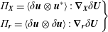
Figure 1. Instantaneous streamwise velocity in an
 $(x,y)$
plane for
$(x,y)$
plane for
 $Re=2500$
in panel (a) and
$Re=2500$
in panel (a) and
 $Re=10\,000$
in panel (b). Single-point turbulent kinetic energy production as a coloured contour plot with the zero mean velocity isoline shown by the dashed line and the boundary of the recirculation bubble shown by the solid line,
$Re=10\,000$
in panel (b). Single-point turbulent kinetic energy production as a coloured contour plot with the zero mean velocity isoline shown by the dashed line and the boundary of the recirculation bubble shown by the solid line,
 $Re=2500$
in panel (c) and
$Re=2500$
in panel (c) and
 $Re=10\,000$
in panel (d).
$Re=10\,000$
in panel (d).
3.2 Flow description
Instantaneous plots of streamwise velocity in an
 $x$
–
$x$
–
 $y$
plane for both low and high Reynolds numbers are shown in figure 1 in (a) and (b) respectively. The incoming flow accelerates at the channel restriction and a recirculating region forms behind the bump, starting downstream of the bump tip. An intense shear layer separates the recirculating region from the outer flow. Downstream of the bump, the flow re-attaches completely. The higher Reynolds number shows a larger range of turbulent scales and the shear layer and recirculating region are smaller and more attached to the bump. Panels (c) and (d) show the turbulent kinetic energy (TKE) production. The flow re-attachment occurs at an earlier
$y$
plane for both low and high Reynolds numbers are shown in figure 1 in (a) and (b) respectively. The incoming flow accelerates at the channel restriction and a recirculating region forms behind the bump, starting downstream of the bump tip. An intense shear layer separates the recirculating region from the outer flow. Downstream of the bump, the flow re-attaches completely. The higher Reynolds number shows a larger range of turbulent scales and the shear layer and recirculating region are smaller and more attached to the bump. Panels (c) and (d) show the turbulent kinetic energy (TKE) production. The flow re-attachment occurs at an earlier
 $x$
position for the higher Reynolds number, as shown by the dividing streamline that separates the recirculation bubble from the outer flow. The effect of the Reynolds number on the turbulence dynamics and energy transfer mechanisms is discussed in detail in Mollicone et al. (Reference Mollicone, Battista, Gualtieri and Casciola2017).
$x$
position for the higher Reynolds number, as shown by the dividing streamline that separates the recirculation bubble from the outer flow. The effect of the Reynolds number on the turbulence dynamics and energy transfer mechanisms is discussed in detail in Mollicone et al. (Reference Mollicone, Battista, Gualtieri and Casciola2017).

Figure 2.
 $Re=2500$
. (a) Flux of kinetic energy of the mean flow
$Re=2500$
. (a) Flux of kinetic energy of the mean flow
 $\unicode[STIX]{x1D74D}_{M}$
(vectors), mean flow dissipation
$\unicode[STIX]{x1D74D}_{M}$
(vectors), mean flow dissipation
 $\unicode[STIX]{x1D700}_{M}$
(solid yellow isolines) and turbulent kinetic energy production
$\unicode[STIX]{x1D700}_{M}$
(solid yellow isolines) and turbulent kinetic energy production
 $\unicode[STIX]{x03C0}$
(coloured contours). (b) Flux of turbulent kinetic energy
$\unicode[STIX]{x03C0}$
(coloured contours). (b) Flux of turbulent kinetic energy
 $\unicode[STIX]{x1D74D}$
(vectors), turbulent kinetic energy dissipation rate
$\unicode[STIX]{x1D74D}$
(vectors), turbulent kinetic energy dissipation rate
 $\unicode[STIX]{x1D700}$
(solid yellow isolines) and turbulent kinetic energy production
$\unicode[STIX]{x1D700}$
(solid yellow isolines) and turbulent kinetic energy production
 $\unicode[STIX]{x03C0}$
(coloured contours). Reprinted from Mollicone et al. (Reference Mollicone, Battista, Gualtieri and Casciola2017). The boundary of the recirculation bubble is shown by the solid black line.
$\unicode[STIX]{x03C0}$
(coloured contours). Reprinted from Mollicone et al. (Reference Mollicone, Battista, Gualtieri and Casciola2017). The boundary of the recirculation bubble is shown by the solid black line.
The shear layer will predominate in the following section since it is the main source of fluctuations. We shall focus on the region of maximum TKE production, shown in the background of panels (c) and (d), with the maxima occurring at
 $x=5.8$
and
$x=5.8$
and
 $x=5.1$
for lower and higher Reynolds number, respectively. For the reader’s convenience, the picture provided by the (single-point) energy balance discussed in Mollicone et al. (Reference Mollicone, Battista, Gualtieri and Casciola2017) is briefly summarised here and reproduced in figure 2. Panel (a) shows the production of TKE
$x=5.1$
for lower and higher Reynolds number, respectively. For the reader’s convenience, the picture provided by the (single-point) energy balance discussed in Mollicone et al. (Reference Mollicone, Battista, Gualtieri and Casciola2017) is briefly summarised here and reproduced in figure 2. Panel (a) shows the production of TKE
 $\unicode[STIX]{x03C0}=-\langle \boldsymbol{u}\otimes \boldsymbol{u}:\unicode[STIX]{x1D735}\boldsymbol{U}\rangle$
which is concentrated in the shear layer separating the recirculation bubble from the outer flow, see also figure 8 displaying the mean velocity field and the dividing streamline. The production
$\unicode[STIX]{x03C0}=-\langle \boldsymbol{u}\otimes \boldsymbol{u}:\unicode[STIX]{x1D735}\boldsymbol{U}\rangle$
which is concentrated in the shear layer separating the recirculation bubble from the outer flow, see also figure 8 displaying the mean velocity field and the dividing streamline. The production
 $\unicode[STIX]{x03C0}$
largely exceeds the mean kinetic energy dissipation rate
$\unicode[STIX]{x03C0}$
largely exceeds the mean kinetic energy dissipation rate
 $\unicode[STIX]{x1D700}_{M}$
so that, in a simplified picture, the local balance of mean flow kinetic energy,
$\unicode[STIX]{x1D700}_{M}$
so that, in a simplified picture, the local balance of mean flow kinetic energy,
 $1/2|\boldsymbol{U}|^{2}$
, can be approximated as
$1/2|\boldsymbol{U}|^{2}$
, can be approximated as
 $\unicode[STIX]{x1D735}\boldsymbol{\cdot }\unicode[STIX]{x1D74D}_{M}\simeq -\unicode[STIX]{x03C0}$
, where
$\unicode[STIX]{x1D735}\boldsymbol{\cdot }\unicode[STIX]{x1D74D}_{M}\simeq -\unicode[STIX]{x03C0}$
, where
 $\unicode[STIX]{x1D74D}_{M}$
is the flux of mean flow kinetic energy. The turbulence is mostly generated through the divergence of the mean flow kinetic energy flux. The divergence of the mean flow kinetic energy is converted to TKE production which is the direct source of the TKE fluxes
$\unicode[STIX]{x1D74D}_{M}$
is the flux of mean flow kinetic energy. The turbulence is mostly generated through the divergence of the mean flow kinetic energy flux. The divergence of the mean flow kinetic energy is converted to TKE production which is the direct source of the TKE fluxes
 $\unicode[STIX]{x1D74D}$
shown in (b). The comparison between TKE production and TKE dissipation rate
$\unicode[STIX]{x1D74D}$
shown in (b). The comparison between TKE production and TKE dissipation rate
 $\langle \unicode[STIX]{x1D700}\rangle$
confirms that we are dealing with a strongly out-of-equilibrium flow. The position of production and dissipation peaks do not coincide and production in the shear layer largely exceeds dissipation. The excess production in the shear layer in part feeds the recirculation bubble and in part sustains the turbulence downstream of the bump through the TKE fluxes
$\langle \unicode[STIX]{x1D700}\rangle$
confirms that we are dealing with a strongly out-of-equilibrium flow. The position of production and dissipation peaks do not coincide and production in the shear layer largely exceeds dissipation. The excess production in the shear layer in part feeds the recirculation bubble and in part sustains the turbulence downstream of the bump through the TKE fluxes
 $\unicode[STIX]{x1D74D}$
. From this picture, the shear layer emerges as the most active turbulent source from which the spatial fluxes originate. We shall see how this picture is confirmed, reinforced and understood in much finer detail by looking at the same process in the combined space of mid-point positions and scales through the use of the GKE.
$\unicode[STIX]{x1D74D}$
. From this picture, the shear layer emerges as the most active turbulent source from which the spatial fluxes originate. We shall see how this picture is confirmed, reinforced and understood in much finer detail by looking at the same process in the combined space of mid-point positions and scales through the use of the GKE.
4 Results

Figure 3. A point in the
 $(Y,r_{x})$
-plane at constant
$(Y,r_{x})$
-plane at constant
 $X=X^{0}$
,
$X=X^{0}$
,
 $Z=Z^{0}$
,
$Z=Z^{0}$
,
 $r_{y}=r_{y}^{0}$
,
$r_{y}=r_{y}^{0}$
,
 $r_{z}=r_{z}^{0}$
(a) corresponds to two points,
$r_{z}=r_{z}^{0}$
(a) corresponds to two points,
 $\tilde{\boldsymbol{x}},\,\boldsymbol{x}$
, of the physical space such that the mid-point
$\tilde{\boldsymbol{x}},\,\boldsymbol{x}$
, of the physical space such that the mid-point
 $\boldsymbol{X}$
is constrained at
$\boldsymbol{X}$
is constrained at
 $X=X^{0}$
,
$X=X^{0}$
,
 $Z=Z^{0}$
and two components of the separation vector
$Z=Z^{0}$
and two components of the separation vector
 $\boldsymbol{r}$
are fixed,
$\boldsymbol{r}$
are fixed,
 $r_{y}=r_{y}^{0},\;r_{z}=r_{z}^{0}$
(b). The red lines sketch the lower wall of the channel and the bump. By moving from
$r_{y}=r_{y}^{0},\;r_{z}=r_{z}^{0}$
(b). The red lines sketch the lower wall of the channel and the bump. By moving from
 $(Y,r_{x})$
to
$(Y,r_{x})$
to
 $(Y+\text{d}Y,r_{x}+\text{d}r_{x})$
the separation vector
$(Y+\text{d}Y,r_{x}+\text{d}r_{x})$
the separation vector
 $\boldsymbol{r}$
(b) changes from the blue to the green one.
$\boldsymbol{r}$
(b) changes from the blue to the green one.
In order to visualise the second-order velocity structure function, it is helpful to consider two-dimensional sections of the five-dimensional phase space
 $(X,Y,r_{x},r_{y},r_{z})$
introduced in § 2. The sketch in figure 3 addresses a typical
$(X,Y,r_{x},r_{y},r_{z})$
introduced in § 2. The sketch in figure 3 addresses a typical
 $(Y,r_{x})$
-plane (section at constant
$(Y,r_{x})$
-plane (section at constant
 $X=X^{0}$
,
$X=X^{0}$
,
 $Z=Z^{0}$
,
$Z=Z^{0}$
,
 $r_{y}=r_{y}^{0}$
and
$r_{y}=r_{y}^{0}$
and
 $r_{z}=r_{z}^{0}$
). It shows the physical space points,
$r_{z}=r_{z}^{0}$
). It shows the physical space points,
 $\tilde{\boldsymbol{x}}$
and
$\tilde{\boldsymbol{x}}$
and
 $\boldsymbol{x}$
, across which the velocity difference is evaluated and the corresponding separation vector
$\boldsymbol{x}$
, across which the velocity difference is evaluated and the corresponding separation vector
 $\boldsymbol{r}$
for two different phase space points in the section. By analogy, the reader may easily figure out the picture for the other planar sections.
$\boldsymbol{r}$
for two different phase space points in the section. By analogy, the reader may easily figure out the picture for the other planar sections.
The isolines of the second-order structure function
 $\langle |\unicode[STIX]{x1D6FF}\boldsymbol{u}|^{2}\rangle$
in four selected phase space planes are plotted in figure 4. We shall focus near the maximum of the effective production of the second-order structure function intensity
$\langle |\unicode[STIX]{x1D6FF}\boldsymbol{u}|^{2}\rangle$
in four selected phase space planes are plotted in figure 4. We shall focus near the maximum of the effective production of the second-order structure function intensity
 $\unicode[STIX]{x1D6F1}_{6}-2\langle \unicode[STIX]{x1D700}^{\ast }\rangle$
. Based on the physical intuition provided by the single-point energy balance discussed in § 3 on the one hand and on the formal theory developed in § 2 on the other, that region (i.e. that range of mid-point positions and separations) is expected to be the source of turbulent fluxes that redistribute turbulent activity across the phase space to different positions
$\unicode[STIX]{x1D6F1}_{6}-2\langle \unicode[STIX]{x1D700}^{\ast }\rangle$
. Based on the physical intuition provided by the single-point energy balance discussed in § 3 on the one hand and on the formal theory developed in § 2 on the other, that region (i.e. that range of mid-point positions and separations) is expected to be the source of turbulent fluxes that redistribute turbulent activity across the phase space to different positions
 $\boldsymbol{X}$
and scales
$\boldsymbol{X}$
and scales
 $\boldsymbol{r}$
. The planes addressed in the four panels actually go through the production maximum. Although not difficult to interpret, the plots are not immediately readable. They will be illustrated in detail in the following discussions regarding the in-plane components of the flux
$\boldsymbol{r}$
. The planes addressed in the four panels actually go through the production maximum. Although not difficult to interpret, the plots are not immediately readable. They will be illustrated in detail in the following discussions regarding the in-plane components of the flux
 $\unicode[STIX]{x1D731}_{\Vert }$
, after a few more details are given on how the four planes shown in figure 4 were selected.
$\unicode[STIX]{x1D731}_{\Vert }$
, after a few more details are given on how the four planes shown in figure 4 were selected.

Figure 4.
 $Re=2500$
. The second-order structure function in different planes. (a)
$Re=2500$
. The second-order structure function in different planes. (a)
 $(Y,r_{x})$
-plane at
$(Y,r_{x})$
-plane at
 $X^{0}=5.8$
,
$X^{0}=5.8$
,
 $r_{y}^{0}=0$
,
$r_{y}^{0}=0$
,
 $r_{z}^{0}=0.4$
. (b)
$r_{z}^{0}=0.4$
. (b)
 $(X,Y)$
-plane at
$(X,Y)$
-plane at
 $r_{x}^{0}=0.45$
,
$r_{x}^{0}=0.45$
,
 $r_{y}^{0}=0$
,
$r_{y}^{0}=0$
,
 $r_{z}^{0}=0.4$
. (c)
$r_{z}^{0}=0.4$
. (c)
 $(Y,r_{y})$
-plane at
$(Y,r_{y})$
-plane at
 $X^{0}=5.8$
,
$X^{0}=5.8$
,
 $r_{x}^{0}=0.45$
,
$r_{x}^{0}=0.45$
,
 $r_{z}^{0}=0.4$
. (d)
$r_{z}^{0}=0.4$
. (d)
 $(X,r_{x})$
-plane at
$(X,r_{x})$
-plane at
 $Y^{0}=0.45$
,
$Y^{0}=0.45$
,
 $r_{y}^{0}=0$
,
$r_{y}^{0}=0$
,
 $r_{z}^{0}=0.4$
. See figure 7 and the related discussion for a description of the yellow symbols.
$r_{z}^{0}=0.4$
. See figure 7 and the related discussion for a description of the yellow symbols.
4.1 Two-dimensional sub-manifold analysis
We need to specify five coordinates to identify the maximum of a function in phase space. Identifying maxima in a five-dimensional space is already non-trivial. In the present case, the issue is more difficult due to the statistical nature of our object. For example, a standard Newton iteration would require the evaluation of the average to be maximised and its five-dimensional gradient at an arbitrary phase space point. Two different strategies may be conceived: either evaluating statistical average and its derivatives at the corresponding coordinate on the fly or having function and derivatives pre-evaluated on a suitable five-dimensional lattice. Both choices are unaffordable given the dimension of the dataset to be manipulated.
As an alternative, we may exploit physical intuition and start by fixing the streamwise coordinate of the mid-point
 $\boldsymbol{X}$
to the cross-stream plane of maximum (single-point) kinetic energy production, namely
$\boldsymbol{X}$
to the cross-stream plane of maximum (single-point) kinetic energy production, namely
 $X^{0}=5.8$
and
$X^{0}=5.8$
and
 $X^{0}=5.1$
for the two cases, § 3. The remaining coordinates,
$X^{0}=5.1$
for the two cases, § 3. The remaining coordinates,
 $Y^{0},r_{x}^{0},r_{y}^{0},r_{z}^{0}$
, will be progressively found from the maxima on selected two-dimensional sub-manifolds. We deliberately choose to fix the streamwise coordinate since the shear layer is elongated in this direction and the dependence on
$Y^{0},r_{x}^{0},r_{y}^{0},r_{z}^{0}$
, will be progressively found from the maxima on selected two-dimensional sub-manifolds. We deliberately choose to fix the streamwise coordinate since the shear layer is elongated in this direction and the dependence on
 $X$
is mild. The emerging picture from slightly different
$X$
is mild. The emerging picture from slightly different
 $X$
sections is therefore negligibly sensitive to the precise location. On the other hand, the dependence on
$X$
sections is therefore negligibly sensitive to the precise location. On the other hand, the dependence on
 $Y$
is strong and requires a careful determination.
$Y$
is strong and requires a careful determination.
Let us take
 $\boldsymbol{r}$
parallel to the streamwise direction,
$\boldsymbol{r}$
parallel to the streamwise direction,
 $\boldsymbol{r}=(r_{x},0,0)$
, keeping in mind that
$\boldsymbol{r}=(r_{x},0,0)$
, keeping in mind that
 $\boldsymbol{X}$
belongs to the fixed cross-stream plane
$\boldsymbol{X}$
belongs to the fixed cross-stream plane
 $X=X^{0}$
. Accounting for translational invariance in the spanwise direction, this manifold is described by the two independent variables
$X=X^{0}$
. Accounting for translational invariance in the spanwise direction, this manifold is described by the two independent variables
 $Y$
and
$Y$
and
 $r_{x}$
(the reader may wish to have a further look at figure 3). We shall therefore first search for the maximum of
$r_{x}$
(the reader may wish to have a further look at figure 3). We shall therefore first search for the maximum of
 $\unicode[STIX]{x1D6F1}_{6}-2\langle \unicode[STIX]{x1D700}^{\ast }\rangle$
in this plane, figure 5(a). The blank areas in the plot correspond to the physical domain boundaries which limit the allowed range of separation vectors. For this specific case, only
$\unicode[STIX]{x1D6F1}_{6}-2\langle \unicode[STIX]{x1D700}^{\ast }\rangle$
in this plane, figure 5(a). The blank areas in the plot correspond to the physical domain boundaries which limit the allowed range of separation vectors. For this specific case, only
 $r_{x}\geqslant 0$
is considered given the
$r_{x}\geqslant 0$
is considered given the
 $r_{x}\rightarrow -r_{x}$
symmetry that holds since
$r_{x}\rightarrow -r_{x}$
symmetry that holds since
 $r_{y},r_{z}$
are still zero. In this plane, the production peak is located at
$r_{y},r_{z}$
are still zero. In this plane, the production peak is located at
 $Y^{0}=0.45$
and
$Y^{0}=0.45$
and
 $r_{x}^{0}=0.45$
. Note that
$r_{x}^{0}=0.45$
. Note that
 $Y^{0}$
corresponds to the distance of the shear layer from the bottom wall,
$Y^{0}$
corresponds to the distance of the shear layer from the bottom wall,
 $y_{sl}=0.45$
.
$y_{sl}=0.45$
.
Figure 5. Contour plots of the net production
 $\unicode[STIX]{x1D6F1}_{6}-2\langle \unicode[STIX]{x1D700}^{\ast }\rangle$
for the dataset at
$\unicode[STIX]{x1D6F1}_{6}-2\langle \unicode[STIX]{x1D700}^{\ast }\rangle$
for the dataset at
 $Re=2500$
. (a) Plane
$Re=2500$
. (a) Plane
 $(Y,r_{x})|_{X=5.8,r_{y}=r_{z}=0}$
; (b) plane
$(Y,r_{x})|_{X=5.8,r_{y}=r_{z}=0}$
; (b) plane
 $(Y,r_{y})|_{X=5.8,r_{x}=r_{z}=0}$
; (c) plane
$(Y,r_{y})|_{X=5.8,r_{x}=r_{z}=0}$
; (c) plane
 $(Y,r_{z})|_{X=5.8,r_{x}=r_{y}=0}$
; (d) plane
$(Y,r_{z})|_{X=5.8,r_{x}=r_{y}=0}$
; (d) plane
 $(Y,r_{y})|_{r_{x}=0.45,r_{z}=0.4}$
.
$(Y,r_{y})|_{r_{x}=0.45,r_{z}=0.4}$
.
Keeping
 $X$
constant and taking the separation vector in the wall-normal direction,
$X$
constant and taking the separation vector in the wall-normal direction,
 $\boldsymbol{r}=(0,r_{y},0)$
, the two independent variables are now
$\boldsymbol{r}=(0,r_{y},0)$
, the two independent variables are now
 $Y$
and
$Y$
and
 $r_{y}$
, panel (b). Although two inclined bands of intense production (to be further discussed in the following) are apparent, a single definite maximum cannot unambiguously be identified in this plane.
$r_{y}$
, panel (b). Although two inclined bands of intense production (to be further discussed in the following) are apparent, a single definite maximum cannot unambiguously be identified in this plane.
For separations in the spanwise direction,
 $\boldsymbol{r}=(0,0,r_{z})$
, the maximum is determined from panel (c). The highest production occurs at
$\boldsymbol{r}=(0,0,r_{z})$
, the maximum is determined from panel (c). The highest production occurs at
 $Y^{0}=0.45$
, again matching the height of the shear layer and, although the isolines are rather elongated, the maximum is found at
$Y^{0}=0.45$
, again matching the height of the shear layer and, although the isolines are rather elongated, the maximum is found at
 $r_{z}^{0}=0.4$
. Instantaneous configurations of the velocity field coinciding with
$r_{z}^{0}=0.4$
. Instantaneous configurations of the velocity field coinciding with
 $x=X^{0}$
and
$x=X^{0}$
and
 $y=Y^{0}$
are shown in figure 6. From panels (a) and (c), a well-defined transversal scale is apparent. The minimum of the transversal correlation coefficient
$y=Y^{0}$
are shown in figure 6. From panels (a) and (c), a well-defined transversal scale is apparent. The minimum of the transversal correlation coefficient
 $R_{z}^{uu}=\langle u(x^{0},y^{0},z)u(x^{0},y^{0},z+r_{z})\rangle /\langle u(x^{0},y^{0},z)^{2}\rangle$
shown in panel (d) identifies this characteristic length scale at the shear layer (red curve) as
$R_{z}^{uu}=\langle u(x^{0},y^{0},z)u(x^{0},y^{0},z+r_{z})\rangle /\langle u(x^{0},y^{0},z)^{2}\rangle$
shown in panel (d) identifies this characteristic length scale at the shear layer (red curve) as
 $L_{T}\simeq 0.42$
. This value is consistent with the transversal scale where the maximum net production occurs
$L_{T}\simeq 0.42$
. This value is consistent with the transversal scale where the maximum net production occurs
 $(r_{z}^{0}=0.4)$
.
$(r_{z}^{0}=0.4)$
.
Figure 6. Instantaneous streamwise velocity contours for
 $Re=2500$
. (a)
$Re=2500$
. (a)
 $(y,z)$
-plane at
$(y,z)$
-plane at
 $x^{0}=5.8$
; (b)
$x^{0}=5.8$
; (b)
 $(x,y)$
-plane at arbitrary
$(x,y)$
-plane at arbitrary
 $z^{0}$
; (c)
$z^{0}$
; (c)
 $(x,z)$
-plane at
$(x,z)$
-plane at
 $y^{0}=0.45$
. Panel (d) shows the spanwise correlation
$y^{0}=0.45$
. Panel (d) shows the spanwise correlation
 $R_{z}^{uu}=\langle u(x^{0},y^{0},z)u(x^{0},y^{0},z+r_{z})/\langle u(x^{0},y^{0},z)\rangle ^{2}\rangle$
for
$R_{z}^{uu}=\langle u(x^{0},y^{0},z)u(x^{0},y^{0},z+r_{z})/\langle u(x^{0},y^{0},z)\rangle ^{2}\rangle$
for
 $x^{0}=5.8$
in the shear layer,
$x^{0}=5.8$
in the shear layer,
 $y^{0}=0.45$
(red) and at the centreline,
$y^{0}=0.45$
(red) and at the centreline,
 $y^{0}=1.0$
(blue).
$y^{0}=1.0$
(blue).
Recalling that
 $r_{y}$
is still undetermined, the plane of panel (b) is relocated, see panel (d) which shows the production in the plane
$r_{y}$
is still undetermined, the plane of panel (b) is relocated, see panel (d) which shows the production in the plane
 $(Y,r_{y})|_{X=5.8,r_{x}=0.45,r_{z}=0.4}$
. The maximum is clearly found at the intersection of the inclined bands at
$(Y,r_{y})|_{X=5.8,r_{x}=0.45,r_{z}=0.4}$
. The maximum is clearly found at the intersection of the inclined bands at
 $Y=0.45$
and
$Y=0.45$
and
 $r_{y}^{0}=0$
.
$r_{y}^{0}=0$
.
All the planes considered so far can now be repositioned: the first one –
 $(Y,r_{x})$
– will now be the plane
$(Y,r_{x})$
– will now be the plane
 $X=X^{0}$
,
$X=X^{0}$
,
 $r_{y}=r_{y}^{0}$
,
$r_{y}=r_{y}^{0}$
,
 $r_{z}=r_{z}^{0}$
, while the second –
$r_{z}=r_{z}^{0}$
, while the second –
 $(Y,r_{y})$
– and the third –
$(Y,r_{y})$
– and the third –
 $(Y,r_{z})$
– will be
$(Y,r_{z})$
– will be
 $X=X^{0}$
,
$X=X^{0}$
,
 $r_{z}=r_{z}^{0}$
,
$r_{z}=r_{z}^{0}$
,
 $r_{x}=r_{x}^{0}$
and
$r_{x}=r_{x}^{0}$
and
 $X=X^{0}$
,
$X=X^{0}$
,
 $r_{x}=r_{x}^{0}$
,
$r_{x}=r_{x}^{0}$
,
 $r_{y}=r_{y}^{0}$
, respectively. Based on this approach, an iterative algorithm that looks for the maxima and updates the planes until convergence could in principle be set-up but, for the present cases, it is found to leave the result essentially unaltered.
$r_{y}=r_{y}^{0}$
, respectively. Based on this approach, an iterative algorithm that looks for the maxima and updates the planes until convergence could in principle be set-up but, for the present cases, it is found to leave the result essentially unaltered.
For the dataset at
 $Re=10\,000$
(not shown), the behaviour is similar but everything occurs closer to the bump since the shear layer, together with the maxima of
$Re=10\,000$
(not shown), the behaviour is similar but everything occurs closer to the bump since the shear layer, together with the maxima of
 $\unicode[STIX]{x1D6F1}_{6}-2\langle \unicode[STIX]{x1D700}^{\ast }\rangle$
, moves towards the bump at increasing Reynolds number as shown in Mollicone et al. (Reference Mollicone, Battista, Gualtieri and Casciola2017).
$\unicode[STIX]{x1D6F1}_{6}-2\langle \unicode[STIX]{x1D700}^{\ast }\rangle$
, moves towards the bump at increasing Reynolds number as shown in Mollicone et al. (Reference Mollicone, Battista, Gualtieri and Casciola2017).
In summary, to a degree of accuracy sufficient for our next discussion, the maximum net production intensity
 $(\unicode[STIX]{x1D6F1}_{6}-2\langle \unicode[STIX]{x1D700}^{\ast }\rangle )_{\max }$
is found at
$(\unicode[STIX]{x1D6F1}_{6}-2\langle \unicode[STIX]{x1D700}^{\ast }\rangle )_{\max }$
is found at
 $X^{0}=5.8$
,
$X^{0}=5.8$
,
 $Y^{0}=0.45$
,
$Y^{0}=0.45$
,
 $r_{x}^{0}=0.45$
,
$r_{x}^{0}=0.45$
,
 $r_{y}^{0}=0.$
and
$r_{y}^{0}=0.$
and
 $r_{z}^{0}=0.4$
for the case at
$r_{z}^{0}=0.4$
for the case at
 $Re=2500$
and at
$Re=2500$
and at
 $X^{0}=5.1$
,
$X^{0}=5.1$
,
 $Y^{0}=0.45$
,
$Y^{0}=0.45$
,
 $r_{x}^{0}=0.17$
,
$r_{x}^{0}=0.17$
,
 $r_{y}^{0}=0.$
and
$r_{y}^{0}=0.$
and
 $r_{z}^{0}=0.13$
for
$r_{z}^{0}=0.13$
for
 $Re=10\,000$
.
$Re=10\,000$
.
As discussed in § 2, a way to represent the five-dimensional fields involved in the GKE consists in selecting two-dimensional planes. Considering, e.g. the
 $(Y,r_{y})$
-plane, the in-plane component of the flux vector
$(Y,r_{y})$
-plane, the in-plane component of the flux vector
 $\unicode[STIX]{x1D731}_{6}$
,
$\unicode[STIX]{x1D731}_{6}$
,
 $\unicode[STIX]{x1D731}_{\Vert }=(\unicode[STIX]{x1D6F7}_{Y},\unicode[STIX]{x1D6F7}_{r_{y}})$
, follows the equation
$\unicode[STIX]{x1D731}_{\Vert }=(\unicode[STIX]{x1D6F7}_{Y},\unicode[STIX]{x1D6F7}_{r_{y}})$
, follows the equation
 $$\begin{eqnarray}\displaystyle & \displaystyle \unicode[STIX]{x1D735}_{\Vert }\boldsymbol{\cdot }\unicode[STIX]{x1D731}_{\Vert }=\unicode[STIX]{x1D6F1}_{6}-2\langle \unicode[STIX]{x1D700}^{\ast }\rangle -\unicode[STIX]{x1D735}_{\bot }\boldsymbol{\cdot }\unicode[STIX]{x1D731}_{\bot }, & \displaystyle\end{eqnarray}$$
where the general six-dimensional gradient is expressed as the sum of in-plane and normal component,
 $\unicode[STIX]{x1D735}_{\Vert }=(\unicode[STIX]{x2202}/\unicode[STIX]{x2202}Y,\unicode[STIX]{x2202}/\unicode[STIX]{x2202}r_{y})$
and
$\unicode[STIX]{x1D735}_{\Vert }=(\unicode[STIX]{x2202}/\unicode[STIX]{x2202}Y,\unicode[STIX]{x2202}/\unicode[STIX]{x2202}r_{y})$
and
 $\unicode[STIX]{x1D735}_{\bot }=(\unicode[STIX]{x2202}/\unicode[STIX]{x2202}X,\unicode[STIX]{x2202}/\unicode[STIX]{x2202}r_{z},\unicode[STIX]{x2202}/\unicode[STIX]{x2202}r_{x})$
, respectively. The actual number of dimensions of the phase space is reduced to five given the invariance to
$\unicode[STIX]{x1D735}_{\bot }=(\unicode[STIX]{x2202}/\unicode[STIX]{x2202}X,\unicode[STIX]{x2202}/\unicode[STIX]{x2202}r_{z},\unicode[STIX]{x2202}/\unicode[STIX]{x2202}r_{x})$
, respectively. The actual number of dimensions of the phase space is reduced to five given the invariance to
 $z$
-translations,
$z$
-translations,
 $\unicode[STIX]{x2202}/\unicode[STIX]{x2202}_{Z}=0$
. Equation (4.1) is obtained from (2.5) after moving the orthogonal components of the flux,
$\unicode[STIX]{x2202}/\unicode[STIX]{x2202}_{Z}=0$
. Equation (4.1) is obtained from (2.5) after moving the orthogonal components of the flux,
 $\unicode[STIX]{x1D731}_{\bot }=(\unicode[STIX]{x1D6F7}_{X},\unicode[STIX]{x1D6F7}_{r_{z}},\unicode[STIX]{x1D6F7}_{r_{x}})$
, to the right-hand side.
$\unicode[STIX]{x1D731}_{\bot }=(\unicode[STIX]{x1D6F7}_{X},\unicode[STIX]{x1D6F7}_{r_{z}},\unicode[STIX]{x1D6F7}_{r_{x}})$
, to the right-hand side.
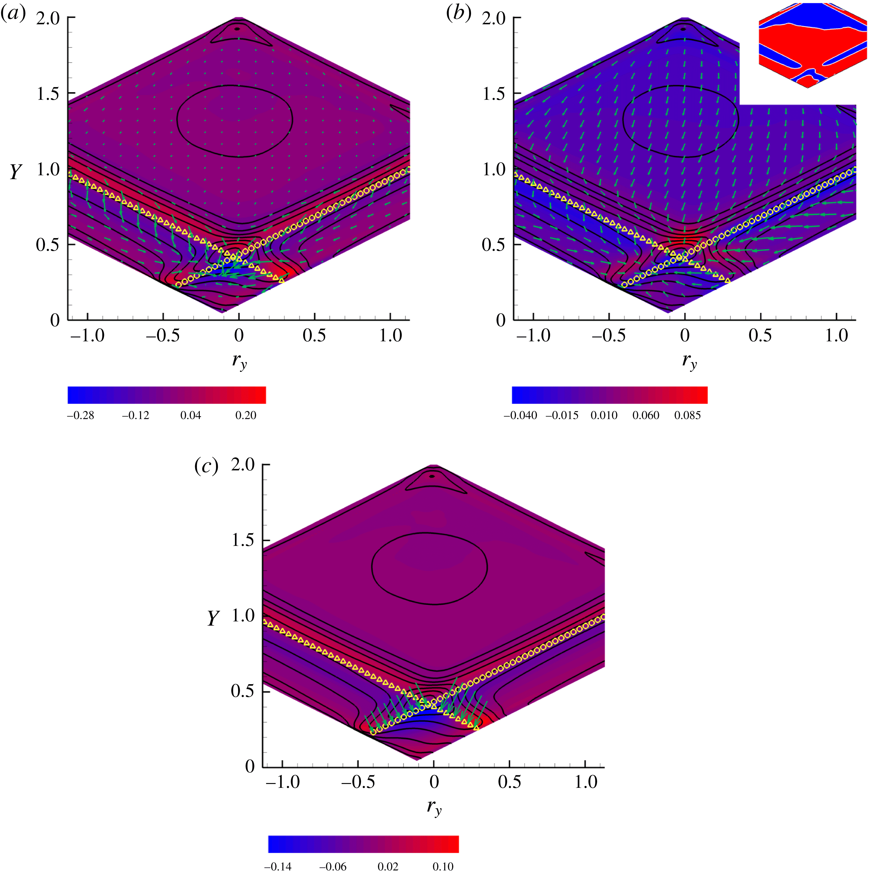
Figure 7.
 $Re=2500$
,
$Re=2500$
,
 $(Y,r_{y})$
-plane at
$(Y,r_{y})$
-plane at
 $X^{0}=5.8$
,
$X^{0}=5.8$
,
 $r_{x}^{0}=0.45$
,
$r_{x}^{0}=0.45$
,
 $r_{z}^{0}=0.4$
. Solid isolines represent
$r_{z}^{0}=0.4$
. Solid isolines represent
 $\langle |\unicode[STIX]{x1D6FF}\boldsymbol{u}|^{2}\rangle$
. (a) In-plane component of the flux
$\langle |\unicode[STIX]{x1D6FF}\boldsymbol{u}|^{2}\rangle$
. (a) In-plane component of the flux
 $\unicode[STIX]{x1D731}_{\Vert }=(\unicode[STIX]{x1D6F7}_{Y},\unicode[STIX]{x1D6F7}_{r_{y}})$
as vectors, equation (2.3). The coloured contour denotes the source terms
$\unicode[STIX]{x1D731}_{\Vert }=(\unicode[STIX]{x1D6F7}_{Y},\unicode[STIX]{x1D6F7}_{r_{y}})$
as vectors, equation (2.3). The coloured contour denotes the source terms
 $\unicode[STIX]{x1D6F1}_{6}-2\langle \unicode[STIX]{x1D700}^{\ast }\rangle -\unicode[STIX]{x1D735}_{\bot }\boldsymbol{\cdot }\unicode[STIX]{x1D731}_{\bot }$
, equation (4.1), where
$\unicode[STIX]{x1D6F1}_{6}-2\langle \unicode[STIX]{x1D700}^{\ast }\rangle -\unicode[STIX]{x1D735}_{\bot }\boldsymbol{\cdot }\unicode[STIX]{x1D731}_{\bot }$
, equation (4.1), where
 $\unicode[STIX]{x1D735}_{\bot }=(\unicode[STIX]{x2202}_{X},\unicode[STIX]{x2202}_{r_{z}},\unicode[STIX]{x2202}_{r_{x}})$
and
$\unicode[STIX]{x1D735}_{\bot }=(\unicode[STIX]{x2202}_{X},\unicode[STIX]{x2202}_{r_{z}},\unicode[STIX]{x2202}_{r_{x}})$
and
 $\unicode[STIX]{x1D731}_{\bot }=(\unicode[STIX]{x1D6F7}_{X},\unicode[STIX]{x1D6F7}_{r_{z}},\unicode[STIX]{x1D6F7}_{r_{x}})$
. (b) In-plane transport velocity
$\unicode[STIX]{x1D731}_{\bot }=(\unicode[STIX]{x1D6F7}_{X},\unicode[STIX]{x1D6F7}_{r_{z}},\unicode[STIX]{x1D6F7}_{r_{x}})$
. (b) In-plane transport velocity
 $\boldsymbol{w}_{\Vert }=(w_{Y},w_{r_{y}})$
as vectors, equation (2.15), and effective net production in the plane
$\boldsymbol{w}_{\Vert }=(w_{Y},w_{r_{y}})$
as vectors, equation (2.15), and effective net production in the plane
 ${\mathcal{M}}$
, equation (4.3), as coloured contour. The yellow symbols denote the images of the bubble separatrix:
${\mathcal{M}}$
, equation (4.3), as coloured contour. The yellow symbols denote the images of the bubble separatrix:
 $f_{b}(\tilde{\boldsymbol{x}})=0$
(triangles,
$f_{b}(\tilde{\boldsymbol{x}})=0$
(triangles,
 $\tilde{\boldsymbol{x}}=\boldsymbol{X}+\boldsymbol{r}$
on the separatrix) and
$\tilde{\boldsymbol{x}}=\boldsymbol{X}+\boldsymbol{r}$
on the separatrix) and
 $f_{b}(\boldsymbol{x})=0$
(circles,
$f_{b}(\boldsymbol{x})=0$
(circles,
 $\boldsymbol{x}=\boldsymbol{X}-\boldsymbol{r}$
on the separatrix). The inset shows where
$\boldsymbol{x}=\boldsymbol{X}-\boldsymbol{r}$
on the separatrix). The inset shows where
 ${\mathcal{M}}$
is positive (red) or negative (blue). (c) Normal component of the in-plane transport contribution
${\mathcal{M}}$
is positive (red) or negative (blue). (c) Normal component of the in-plane transport contribution
 $\boldsymbol{w}_{\Vert }1/2\langle |\unicode[STIX]{x1D6FF}\boldsymbol{u}|^{2}\rangle$
to the flux (vectors) shown on the bubble separatrix. Coloured contour shows
$\boldsymbol{w}_{\Vert }1/2\langle |\unicode[STIX]{x1D6FF}\boldsymbol{u}|^{2}\rangle$
to the flux (vectors) shown on the bubble separatrix. Coloured contour shows
 $\tilde{{\mathcal{M}}}$
, equation (4.5).
$\tilde{{\mathcal{M}}}$
, equation (4.5).
4.2 Sub-manifold
 $(Y,r_{y})$

Figure 7(a) shows
 $\unicode[STIX]{x1D731}_{\Vert }$
in the
$\unicode[STIX]{x1D731}_{\Vert }$
in the
 $(Y,r_{y})_{X^{0}=5.8,r_{x}^{0}=0.45,r_{z}^{0}=0.4}$
-plane which passes through the maximum of net production. A surface in the ordinary three-dimensional space,
$(Y,r_{y})_{X^{0}=5.8,r_{x}^{0}=0.45,r_{z}^{0}=0.4}$
-plane which passes through the maximum of net production. A surface in the ordinary three-dimensional space,
 $f(\boldsymbol{x})=0$
, generates two images in phase space depending on which one of the two points,
$f(\boldsymbol{x})=0$
, generates two images in phase space depending on which one of the two points,
 $\tilde{\boldsymbol{x}}$
or
$\tilde{\boldsymbol{x}}$
or
 $\boldsymbol{x}$
, belongs to the surface, e.g.
$\boldsymbol{x}$
, belongs to the surface, e.g.
 $f(\tilde{\boldsymbol{x}}/\boldsymbol{x})=f(\boldsymbol{X}\pm \boldsymbol{r}/2)=0$
. The diamond shaped region of the plot is delimited below by the two images of the (curved) lower wall,
$f(\tilde{\boldsymbol{x}}/\boldsymbol{x})=f(\boldsymbol{X}\pm \boldsymbol{r}/2)=0$
. The diamond shaped region of the plot is delimited below by the two images of the (curved) lower wall,
 $f_{lw}(\tilde{\boldsymbol{x}}/\boldsymbol{x})=0$
, and above by those of the (straight) upper wall of the channel,
$f_{lw}(\tilde{\boldsymbol{x}}/\boldsymbol{x})=0$
, and above by those of the (straight) upper wall of the channel,
 $f_{uw}(\tilde{\boldsymbol{x}}/\boldsymbol{x})=0$
. Since the section is taken at
$f_{uw}(\tilde{\boldsymbol{x}}/\boldsymbol{x})=0$
. Since the section is taken at
 $r_{x}^{0}\neq 0$
, the lower boundary of the phase space domain is asymmetric due to the presence of the bump. In the figure, the two curves highlighted with the yellow symbols represent the loci in the
$r_{x}^{0}\neq 0$
, the lower boundary of the phase space domain is asymmetric due to the presence of the bump. In the figure, the two curves highlighted with the yellow symbols represent the loci in the
 $(Y,r_{y})$
-plane corresponding to either
$(Y,r_{y})$
-plane corresponding to either
 $\tilde{\boldsymbol{x}}$
or
$\tilde{\boldsymbol{x}}$
or
 $\boldsymbol{x}$
belonging to the separatrix defining the recirculation bubble, i.e. solid line in figure 8. In physical space, the separatrix is defined by an equation of the form
$\boldsymbol{x}$
belonging to the separatrix defining the recirculation bubble, i.e. solid line in figure 8. In physical space, the separatrix is defined by an equation of the form
 $f_{b}(\boldsymbol{x})=0$
or equivalently, given the translational invariance in the
$f_{b}(\boldsymbol{x})=0$
or equivalently, given the translational invariance in the
 $z$
direction,
$z$
direction,
 $y=g_{b}(x)$
. When
$y=g_{b}(x)$
. When
 $\tilde{\boldsymbol{x}}$
is on the separatrix,
$\tilde{\boldsymbol{x}}$
is on the separatrix,
 $f_{b}(\tilde{\boldsymbol{x}})=0$
, i.e.
$f_{b}(\tilde{\boldsymbol{x}})=0$
, i.e.
 $f_{b}(\boldsymbol{X}+\boldsymbol{r}/2)=0$
since
$f_{b}(\boldsymbol{X}+\boldsymbol{r}/2)=0$
since
 $\tilde{\boldsymbol{x}}=\boldsymbol{X}+\boldsymbol{r}/2$
. It is assumed that
$\tilde{\boldsymbol{x}}=\boldsymbol{X}+\boldsymbol{r}/2$
. It is assumed that
 $f_{b}<0$
identifies the region
$f_{b}<0$
identifies the region
 ${\mathcal{B}}$
inside the recirculating bubble. Analogously, when the second of the two points across which the structure function is evaluated belongs to the separatrix,
${\mathcal{B}}$
inside the recirculating bubble. Analogously, when the second of the two points across which the structure function is evaluated belongs to the separatrix,
 $f_{b}(\boldsymbol{X}-\boldsymbol{r}/2)=0$
. The two manifolds
$f_{b}(\boldsymbol{X}-\boldsymbol{r}/2)=0$
. The two manifolds
 $f_{b}(\boldsymbol{X}\pm \boldsymbol{r}/2)=0$
split the phase space into four regions, namely
$f_{b}(\boldsymbol{X}\pm \boldsymbol{r}/2)=0$
split the phase space into four regions, namely
 ${\mathcal{D}}_{II}=\{\boldsymbol{X}(\tilde{\boldsymbol{x}},\boldsymbol{x}),\boldsymbol{r}(\tilde{\boldsymbol{x}},\boldsymbol{x}):\tilde{\boldsymbol{x}},\boldsymbol{x}\in {\mathcal{B}}\}$
, where both
${\mathcal{D}}_{II}=\{\boldsymbol{X}(\tilde{\boldsymbol{x}},\boldsymbol{x}),\boldsymbol{r}(\tilde{\boldsymbol{x}},\boldsymbol{x}):\tilde{\boldsymbol{x}},\boldsymbol{x}\in {\mathcal{B}}\}$
, where both
 $\tilde{\boldsymbol{x}}$
and
$\tilde{\boldsymbol{x}}$
and
 $\boldsymbol{x}$
are inside the bubble,
$\boldsymbol{x}$
are inside the bubble,
 ${\mathcal{D}}_{IO}=\{\boldsymbol{X}(\tilde{\boldsymbol{x}},\boldsymbol{x}),\boldsymbol{r}(\tilde{\boldsymbol{x}},\boldsymbol{x}):\tilde{\boldsymbol{x}}\in {\mathcal{B}},\boldsymbol{x}\notin {\mathcal{B}}\}$
, where only
${\mathcal{D}}_{IO}=\{\boldsymbol{X}(\tilde{\boldsymbol{x}},\boldsymbol{x}),\boldsymbol{r}(\tilde{\boldsymbol{x}},\boldsymbol{x}):\tilde{\boldsymbol{x}}\in {\mathcal{B}},\boldsymbol{x}\notin {\mathcal{B}}\}$
, where only
 $\boldsymbol{x}$
is outside
$\boldsymbol{x}$
is outside
 ${\mathcal{B}}$
,
${\mathcal{B}}$
,
 ${\mathcal{D}}_{OI}=\{\boldsymbol{X}(\tilde{\boldsymbol{x}},\boldsymbol{x}),\boldsymbol{r}(\tilde{\boldsymbol{x}},\boldsymbol{x}):\tilde{\boldsymbol{x}}\notin {\mathcal{B}},\boldsymbol{x}\in {\mathcal{B}}\}$
, where only
${\mathcal{D}}_{OI}=\{\boldsymbol{X}(\tilde{\boldsymbol{x}},\boldsymbol{x}),\boldsymbol{r}(\tilde{\boldsymbol{x}},\boldsymbol{x}):\tilde{\boldsymbol{x}}\notin {\mathcal{B}},\boldsymbol{x}\in {\mathcal{B}}\}$
, where only
 $\tilde{\boldsymbol{x}}$
is outside
$\tilde{\boldsymbol{x}}$
is outside
 ${\mathcal{B}}$
, and
${\mathcal{B}}$
, and
 ${\mathcal{D}}_{OO}=\{\boldsymbol{X}(\tilde{\boldsymbol{x}},\boldsymbol{x}),\boldsymbol{r}(\tilde{\boldsymbol{x}},\boldsymbol{x}):\tilde{\boldsymbol{x}}\notin {\mathcal{B}},\boldsymbol{x}\notin {\mathcal{B}}\}$
, where both
${\mathcal{D}}_{OO}=\{\boldsymbol{X}(\tilde{\boldsymbol{x}},\boldsymbol{x}),\boldsymbol{r}(\tilde{\boldsymbol{x}},\boldsymbol{x}):\tilde{\boldsymbol{x}}\notin {\mathcal{B}},\boldsymbol{x}\notin {\mathcal{B}}\}$
, where both
 $\tilde{\boldsymbol{x}}$
and
$\tilde{\boldsymbol{x}}$
and
 $\boldsymbol{x}$
are outside
$\boldsymbol{x}$
are outside
 ${\mathcal{B}}$
.
${\mathcal{B}}$
.
In the
 $(Y,r_{y})$
-plane, shown in figure 7(a), the traces of the two manifolds reduce to the two (straight) curves
$(Y,r_{y})$
-plane, shown in figure 7(a), the traces of the two manifolds reduce to the two (straight) curves
 $Y=g_{b}(X^{0}\pm r_{x}^{0}/2)\mp r_{y}/2$
shown by the yellow symbols in the plot, where triangles show the trace of the manifold
$Y=g_{b}(X^{0}\pm r_{x}^{0}/2)\mp r_{y}/2$
shown by the yellow symbols in the plot, where triangles show the trace of the manifold
 $f_{b}(\tilde{\boldsymbol{x}})=0$
whilst circles correspond to
$f_{b}(\tilde{\boldsymbol{x}})=0$
whilst circles correspond to
 $f_{b}(\boldsymbol{x})=0$
. The solid isolines show the magnitude of the second-order structure function
$f_{b}(\boldsymbol{x})=0$
. The solid isolines show the magnitude of the second-order structure function
 $\langle |\unicode[STIX]{x1D6FF}\boldsymbol{u}|^{2}\rangle$
of figure 4(c), the colour background gives the isolevels of the right-hand side of (4.1) (dubbed the source in the following description) whilst vectors represent
$\langle |\unicode[STIX]{x1D6FF}\boldsymbol{u}|^{2}\rangle$
of figure 4(c), the colour background gives the isolevels of the right-hand side of (4.1) (dubbed the source in the following description) whilst vectors represent
 $\unicode[STIX]{x1D731}_{\Vert }$
. Just above the two images of the separatrix, inside
$\unicode[STIX]{x1D731}_{\Vert }$
. Just above the two images of the separatrix, inside
 ${\mathcal{D}}_{OO}$
, the two elongated regions of intense source correspond to the shear layer. The in-plane flux
${\mathcal{D}}_{OO}$
, the two elongated regions of intense source correspond to the shear layer. The in-plane flux
 $\unicode[STIX]{x1D731}_{\Vert }$
in these regions is directed toward decreasing mid-point wall distance
$\unicode[STIX]{x1D731}_{\Vert }$
in these regions is directed toward decreasing mid-point wall distance
 $Y$
and decreasing wall-normal separations
$Y$
and decreasing wall-normal separations
 $r_{y}$
. The physical interpretation of this process will be provided later, after a more complete description of the flow in the phase space. Two (almost) symmetric spots of intense source are observed where the images of the separatrix touch the images of the walls (the one on the left is located around the intersection at
$r_{y}$
. The physical interpretation of this process will be provided later, after a more complete description of the flow in the phase space. Two (almost) symmetric spots of intense source are observed where the images of the separatrix touch the images of the walls (the one on the left is located around the intersection at
 $Y\simeq 0.25$
,
$Y\simeq 0.25$
,
 $r_{y}\simeq -0.45$
, solution of the equation
$r_{y}\simeq -0.45$
, solution of the equation
 $g_{b}(X^{0}-r_{x}^{0}/2)+r_{y}/2=g_{w}(X^{0}+r_{x}^{0}/2)-r_{y}/2$
, where
$g_{b}(X^{0}-r_{x}^{0}/2)+r_{y}/2=g_{w}(X^{0}+r_{x}^{0}/2)-r_{y}/2$
, where
 $y=g_{w}(x)$
is the explicit equation of the lower channel wall, implicitly described by
$y=g_{w}(x)$
is the explicit equation of the lower channel wall, implicitly described by
 $f_{lw}(\boldsymbol{x})$
). In the high intensity red spot on the left, the point
$f_{lw}(\boldsymbol{x})$
). In the high intensity red spot on the left, the point
 $\boldsymbol{x}$
is outside the bubble and within the shear layer (phase space region above the yellow circles). The other point,
$\boldsymbol{x}$
is outside the bubble and within the shear layer (phase space region above the yellow circles). The other point,
 $\tilde{\boldsymbol{x}}$
, is inside the bubble (below the yellow triangles) and close to the wall. An almost symmetric arrangement is found for the right spot. The absolute maximum of the source is found when both
$\tilde{\boldsymbol{x}}$
, is inside the bubble (below the yellow triangles) and close to the wall. An almost symmetric arrangement is found for the right spot. The absolute maximum of the source is found when both
 $\tilde{\boldsymbol{x}}$
and
$\tilde{\boldsymbol{x}}$
and
 $\boldsymbol{x}$
are in the shear layer, just above the intersection of the two images of the separatrix. On the other hand, in the region
$\boldsymbol{x}$
are in the shear layer, just above the intersection of the two images of the separatrix. On the other hand, in the region
 ${\mathcal{D}}_{II}$
(the rhomboidal region limited by lower wall and separatrix) a negative source is present. The fluxes enter this region from outside. The integration of (2.5) over the phase space domain
${\mathcal{D}}_{II}$
(the rhomboidal region limited by lower wall and separatrix) a negative source is present. The fluxes enter this region from outside. The integration of (2.5) over the phase space domain
 ${\mathcal{D}}_{II}$
leads to
${\mathcal{D}}_{II}$
leads to
 $$\begin{eqnarray}\displaystyle & \displaystyle \oint _{\unicode[STIX]{x2202}{\mathcal{D}}_{II}}\unicode[STIX]{x1D731}_{6}\boldsymbol{\cdot }\unicode[STIX]{x1D742}_{6}\,\text{d}S_{6}=\int _{{\mathcal{D}}_{II}}(\unicode[STIX]{x1D6F1}_{6}-2\langle \unicode[STIX]{x1D700}^{\ast }\rangle )\,\text{d}^{3}\boldsymbol{X}\,\text{d}^{3}\boldsymbol{r}. & \displaystyle\end{eqnarray}$$
In the physical sense, the bubble is expected to be of dissipative nature, hence one would guess
 $\unicode[STIX]{x1D6F1}_{6}-2\langle \unicode[STIX]{x1D700}^{\ast }\rangle <0$
. Clearly, the sign of
$\unicode[STIX]{x1D6F1}_{6}-2\langle \unicode[STIX]{x1D700}^{\ast }\rangle <0$
. Clearly, the sign of
 $\unicode[STIX]{x1D6F1}_{6}-2\langle \unicode[STIX]{x1D700}^{\ast }\rangle$
in the entire five-dimensional domain corresponding to the bubble could not be directly checked. However, two-dimensional sections of such domain, like the one shown in figure 7(a), see also the successive figures 9, 10, 11 and 12, suggest that this is indeed the case. This confirms that, being the bubble a statistically steady dissipative feature, the second-order structure function in the bubble region is sustained in time by fluxes entering the domain.
$\unicode[STIX]{x1D6F1}_{6}-2\langle \unicode[STIX]{x1D700}^{\ast }\rangle$
in the entire five-dimensional domain corresponding to the bubble could not be directly checked. However, two-dimensional sections of such domain, like the one shown in figure 7(a), see also the successive figures 9, 10, 11 and 12, suggest that this is indeed the case. This confirms that, being the bubble a statistically steady dissipative feature, the second-order structure function in the bubble region is sustained in time by fluxes entering the domain.
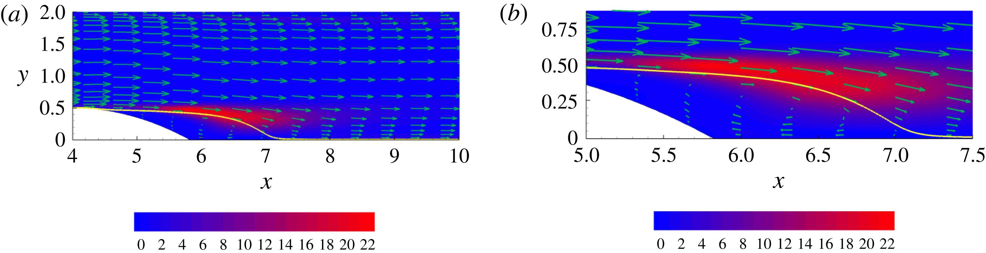
Figure 8.
 $Re=2500$
, (a) Mean velocity field near the bump. Coloured contour denotes the (single-point) TKE production. (b) Enlargement of the recirculating region. The solid line is the stream line separating the bubble from the outer flow.
$Re=2500$
, (a) Mean velocity field near the bump. Coloured contour denotes the (single-point) TKE production. (b) Enlargement of the recirculating region. The solid line is the stream line separating the bubble from the outer flow.
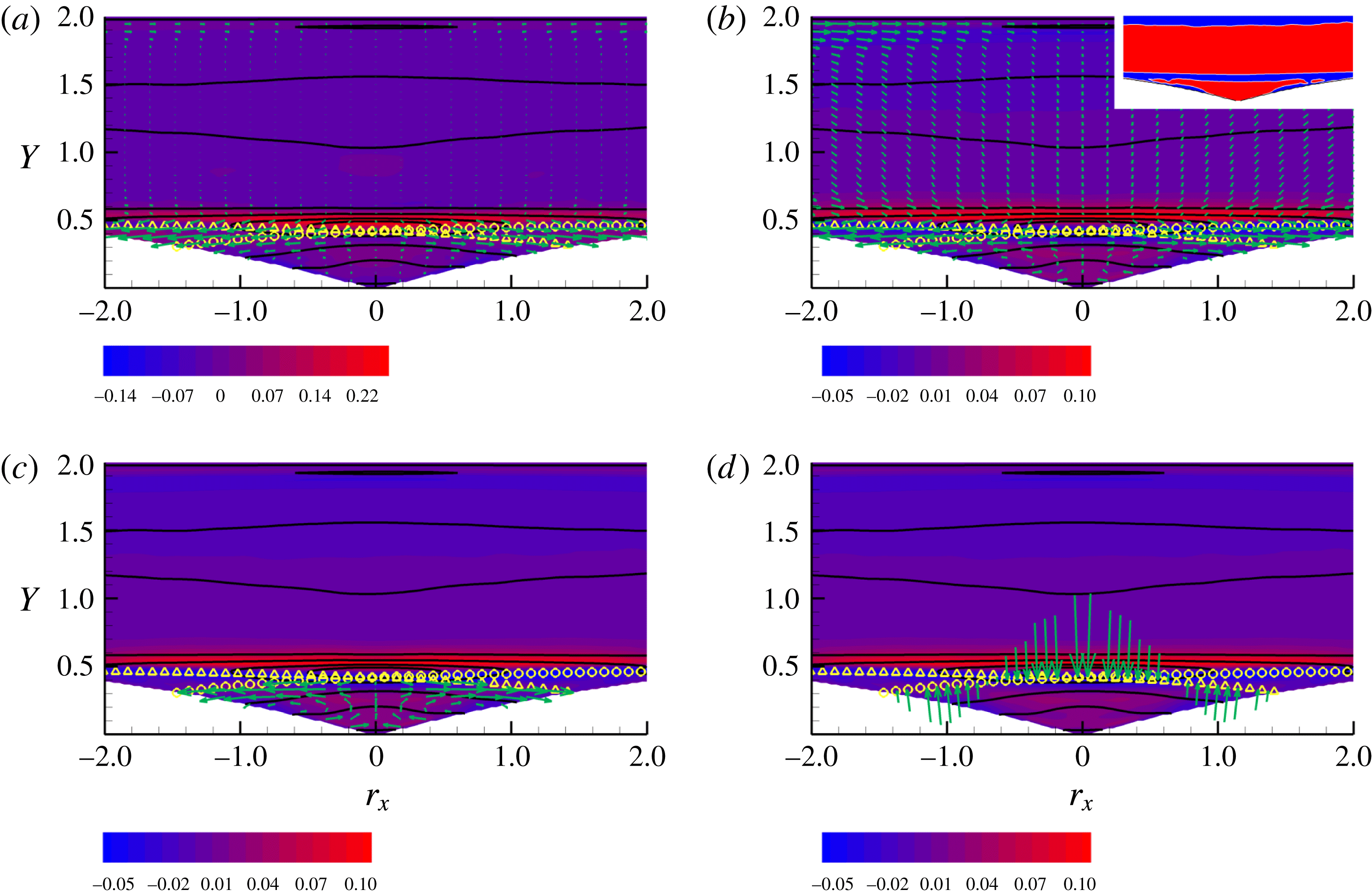
Figure 9.
 $Re=2500$
,
$Re=2500$
,
 $(Y,r_{x})$
-plane at
$(Y,r_{x})$
-plane at
 $X^{0}=5.8$
,
$X^{0}=5.8$
,
 $r_{y}^{0}=0$
,
$r_{y}^{0}=0$
,
 $r_{z}^{0}=0.4$
. In this plane
$r_{z}^{0}=0.4$
. In this plane
 $\unicode[STIX]{x1D735}_{\Vert }=(\unicode[STIX]{x2202}_{Y},\unicode[STIX]{x2202}_{r_{x}})$
. Solid isolines represent
$\unicode[STIX]{x1D735}_{\Vert }=(\unicode[STIX]{x2202}_{Y},\unicode[STIX]{x2202}_{r_{x}})$
. Solid isolines represent
 $\langle |\unicode[STIX]{x1D6FF}\boldsymbol{u}|^{2}\rangle$
. (a) In-plane component of the flux
$\langle |\unicode[STIX]{x1D6FF}\boldsymbol{u}|^{2}\rangle$
. (a) In-plane component of the flux
 $\unicode[STIX]{x1D731}_{\Vert }=(\unicode[STIX]{x1D6F7}_{Y},\unicode[STIX]{x1D6F7}_{r_{x}})$
as vectors, equation (2.3). Coloured contour denotes the source terms
$\unicode[STIX]{x1D731}_{\Vert }=(\unicode[STIX]{x1D6F7}_{Y},\unicode[STIX]{x1D6F7}_{r_{x}})$
as vectors, equation (2.3). Coloured contour denotes the source terms
 $\unicode[STIX]{x1D6F1}_{6}-2\langle \unicode[STIX]{x1D700}^{\ast }\rangle -\unicode[STIX]{x1D735}_{\bot }\boldsymbol{\cdot }\unicode[STIX]{x1D731}_{\bot }$
, equation (4.1), where
$\unicode[STIX]{x1D6F1}_{6}-2\langle \unicode[STIX]{x1D700}^{\ast }\rangle -\unicode[STIX]{x1D735}_{\bot }\boldsymbol{\cdot }\unicode[STIX]{x1D731}_{\bot }$
, equation (4.1), where
 $\unicode[STIX]{x1D735}_{\bot }=(\unicode[STIX]{x2202}_{X},\unicode[STIX]{x2202}_{r_{y}},\unicode[STIX]{x2202}_{r_{z}})$
and
$\unicode[STIX]{x1D735}_{\bot }=(\unicode[STIX]{x2202}_{X},\unicode[STIX]{x2202}_{r_{y}},\unicode[STIX]{x2202}_{r_{z}})$
and
 $\unicode[STIX]{x1D731}_{\bot }=(\unicode[STIX]{x1D6F7}_{X},\unicode[STIX]{x1D6F7}_{r_{y}},\unicode[STIX]{x1D6F7}_{r_{z}})$
. (b) In-plane transport velocity
$\unicode[STIX]{x1D731}_{\bot }=(\unicode[STIX]{x1D6F7}_{X},\unicode[STIX]{x1D6F7}_{r_{y}},\unicode[STIX]{x1D6F7}_{r_{z}})$
. (b) In-plane transport velocity
 $\boldsymbol{w}_{\Vert }=(w_{Y},w_{r_{x}})$
as vectors, equation (2.15) and effective net production in the plane
$\boldsymbol{w}_{\Vert }=(w_{Y},w_{r_{x}})$
as vectors, equation (2.15) and effective net production in the plane
 ${\mathcal{M}}$
, equation (4.3), as coloured contour. The yellow symbols denote the images of the bubble separatrix, see text and figure 7. The inset shows the sign of
${\mathcal{M}}$
, equation (4.3), as coloured contour. The yellow symbols denote the images of the bubble separatrix, see text and figure 7. The inset shows the sign of
 ${\mathcal{M}}$
. (c) Same as (a) with the in-plane velocity magnified in the region
${\mathcal{M}}$
. (c) Same as (a) with the in-plane velocity magnified in the region
 ${\mathcal{D}}_{II}^{\Vert }$
, see text. (d) Normal component of the in-plane transport contribution
${\mathcal{D}}_{II}^{\Vert }$
, see text. (d) Normal component of the in-plane transport contribution
 $\boldsymbol{w}_{\Vert }1/2\langle |\unicode[STIX]{x1D6FF}\boldsymbol{u}|^{2}\rangle$
to the flux (vectors) shown on the bubble separatrix. Coloured contour shows
$\boldsymbol{w}_{\Vert }1/2\langle |\unicode[STIX]{x1D6FF}\boldsymbol{u}|^{2}\rangle$
to the flux (vectors) shown on the bubble separatrix. Coloured contour shows
 $\tilde{{\mathcal{M}}}$
, equation (4.5).
$\tilde{{\mathcal{M}}}$
, equation (4.5).
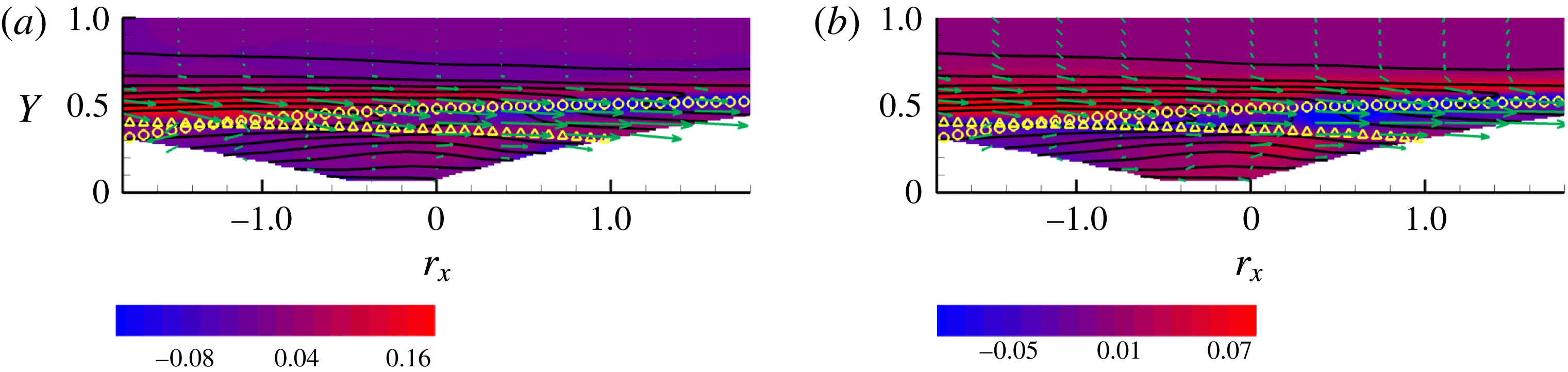
Figure 10.
 $Re=2500$
,
$Re=2500$
,
 $(Y,r_{x})$
-plane at
$(Y,r_{x})$
-plane at
 $X^{0}=5.8$
,
$X^{0}=5.8$
,
 $r_{y}^{0}=0.12$
,
$r_{y}^{0}=0.12$
,
 $r_{z}^{0}=0.4$
. Panels (a) and (b) same as corresponding panels of figure 9.
$r_{z}^{0}=0.4$
. Panels (a) and (b) same as corresponding panels of figure 9.
The Lagrangian theory in § 2.2 allows us to define a velocity field
 $\boldsymbol{w}_{6}$
which transports the structure function in phase space. This, in a way, provides the phase space equivalent of the advection of fluid particles by the velocity field in physical space. Again, the transport velocity field defined in (2.14), (2.15) is not easily visualised. Planar sections can provide an illuminating, though admittedly incomplete, view. In a planar section, the transport (2.16), (2.17) for the structure function can be rearranged as
$\boldsymbol{w}_{6}$
which transports the structure function in phase space. This, in a way, provides the phase space equivalent of the advection of fluid particles by the velocity field in physical space. Again, the transport velocity field defined in (2.14), (2.15) is not easily visualised. Planar sections can provide an illuminating, though admittedly incomplete, view. In a planar section, the transport (2.16), (2.17) for the structure function can be rearranged as
 $$\begin{eqnarray}\displaystyle & \displaystyle \frac{\text{D}_{\Vert }}{\text{D}t}\left(\frac{1}{2}\langle |\unicode[STIX]{x1D6FF}\boldsymbol{u}|^{2}\rangle \right)={\mathcal{M}}, & \displaystyle\end{eqnarray}$$
where
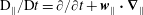 $\text{D}_{\Vert }/\text{D}t=\unicode[STIX]{x2202}/\unicode[STIX]{x2202}t+\boldsymbol{w}_{\Vert }\boldsymbol{\cdot }\unicode[STIX]{x1D735}_{\Vert }$
is the transport derivative in the plane (
$\text{D}_{\Vert }/\text{D}t=\unicode[STIX]{x2202}/\unicode[STIX]{x2202}t+\boldsymbol{w}_{\Vert }\boldsymbol{\cdot }\unicode[STIX]{x1D735}_{\Vert }$
is the transport derivative in the plane (
 $\unicode[STIX]{x2202}/\unicode[STIX]{x2202}t=0$
for the present statistically steady conditions) and the source term on the right-hand side is
$\unicode[STIX]{x2202}/\unicode[STIX]{x2202}t=0$
for the present statistically steady conditions) and the source term on the right-hand side is
 $$\begin{eqnarray}\displaystyle & \displaystyle {\mathcal{M}}=\unicode[STIX]{x1D6F1}_{6}-2\langle \unicode[STIX]{x1D700}^{\ast }\rangle -\unicode[STIX]{x1D735}_{\bot }\boldsymbol{\cdot }\unicode[STIX]{x1D731}_{\bot }-\unicode[STIX]{x1D735}_{\Vert }\boldsymbol{\cdot }\unicode[STIX]{x1D731}_{\Vert }^{D}-{\textstyle \frac{1}{2}}\langle |\unicode[STIX]{x1D6FF}\boldsymbol{u}|^{2}\rangle \unicode[STIX]{x1D735}_{\Vert }\boldsymbol{\cdot }\boldsymbol{w}_{\Vert }, & \displaystyle\end{eqnarray}$$
with the superscript
 $D$
denoting diffusion, equation (2.6). The transport velocity
$D$
denoting diffusion, equation (2.6). The transport velocity
 $\boldsymbol{w}_{\Vert }=(w_{Y},w_{r_{y}})$
in the
$\boldsymbol{w}_{\Vert }=(w_{Y},w_{r_{y}})$
in the
 $(Y,r_{y})$
-plane is shown in figure 7(b). As in panel (a), the solid isolines represent the structure function and the yellow symbols the two images of the separatrix. The colour contours now provide
$(Y,r_{y})$
-plane is shown in figure 7(b). As in panel (a), the solid isolines represent the structure function and the yellow symbols the two images of the separatrix. The colour contours now provide
 ${\mathcal{M}}$
, the right-hand side of (4.3), explicitly defined in (4.4). The inset highlights the zero isolevel of
${\mathcal{M}}$
, the right-hand side of (4.3), explicitly defined in (4.4). The inset highlights the zero isolevel of
 ${\mathcal{M}}$
, with red and blue denoting positive and negative values respectively.
${\mathcal{M}}$
, with red and blue denoting positive and negative values respectively.

Figure 11.
 $Re=2500$
,
$Re=2500$
,
 $(X,r_{x})$
-plane at
$(X,r_{x})$
-plane at
 $Y^{0}=0.45$
,
$Y^{0}=0.45$
,
 $r_{y}^{0}=0$
,
$r_{y}^{0}=0$
,
 $r_{z}^{0}=0.4$
. In this plane
$r_{z}^{0}=0.4$
. In this plane
 $\unicode[STIX]{x1D735}_{\Vert }=(\unicode[STIX]{x2202}_{X},\unicode[STIX]{x2202}_{r_{x}})$
. Solid isolines represent
$\unicode[STIX]{x1D735}_{\Vert }=(\unicode[STIX]{x2202}_{X},\unicode[STIX]{x2202}_{r_{x}})$
. Solid isolines represent
 $\langle |\unicode[STIX]{x1D6FF}\boldsymbol{u}|^{2}\rangle$
. (a) In-plane component of the flux
$\langle |\unicode[STIX]{x1D6FF}\boldsymbol{u}|^{2}\rangle$
. (a) In-plane component of the flux
 $\unicode[STIX]{x1D731}_{\Vert }=(\unicode[STIX]{x1D6F7}_{X},\unicode[STIX]{x1D6F7}_{r_{x}})$
as vectors, equation (2.3). Coloured contour denotes the source terms
$\unicode[STIX]{x1D731}_{\Vert }=(\unicode[STIX]{x1D6F7}_{X},\unicode[STIX]{x1D6F7}_{r_{x}})$
as vectors, equation (2.3). Coloured contour denotes the source terms
 $\unicode[STIX]{x1D6F1}_{6}-2\langle \unicode[STIX]{x1D700}^{\ast }\rangle -\unicode[STIX]{x1D735}_{\bot }\boldsymbol{\cdot }\unicode[STIX]{x1D731}_{\bot }$
, equation (4.1), where
$\unicode[STIX]{x1D6F1}_{6}-2\langle \unicode[STIX]{x1D700}^{\ast }\rangle -\unicode[STIX]{x1D735}_{\bot }\boldsymbol{\cdot }\unicode[STIX]{x1D731}_{\bot }$
, equation (4.1), where
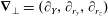 $\unicode[STIX]{x1D735}_{\bot }=(\unicode[STIX]{x2202}_{Y},\unicode[STIX]{x2202}_{r_{y}},\unicode[STIX]{x2202}_{r_{z}})$
and
$\unicode[STIX]{x1D735}_{\bot }=(\unicode[STIX]{x2202}_{Y},\unicode[STIX]{x2202}_{r_{y}},\unicode[STIX]{x2202}_{r_{z}})$
and
 $\unicode[STIX]{x1D731}_{\bot }=(\unicode[STIX]{x1D6F7}_{Y},\unicode[STIX]{x1D6F7}_{r_{y}},\unicode[STIX]{x1D6F7}_{r_{z}})$
. (b) In-plane transport velocity
$\unicode[STIX]{x1D731}_{\bot }=(\unicode[STIX]{x1D6F7}_{Y},\unicode[STIX]{x1D6F7}_{r_{y}},\unicode[STIX]{x1D6F7}_{r_{z}})$
. (b) In-plane transport velocity
 $\boldsymbol{w}_{\Vert }=(w_{X},w_{r_{x}})$
as vectors, equation (2.15) and effective net production in the plane
$\boldsymbol{w}_{\Vert }=(w_{X},w_{r_{x}})$
as vectors, equation (2.15) and effective net production in the plane
 ${\mathcal{M}}$
, equation (4.3), as coloured contour. The inset shows the sign of
${\mathcal{M}}$
, equation (4.3), as coloured contour. The inset shows the sign of
 ${\mathcal{M}}$
. The yellow symbols denote the images of the bubble separatrix, see text and figure 7. (c) Same as (a) with the in-plane velocity magnified in the region
${\mathcal{M}}$
. The yellow symbols denote the images of the bubble separatrix, see text and figure 7. (c) Same as (a) with the in-plane velocity magnified in the region
 ${\mathcal{D}}_{II}^{\Vert }$
, see text. (d) Normal component of the in-plane transport contribution
${\mathcal{D}}_{II}^{\Vert }$
, see text. (d) Normal component of the in-plane transport contribution
 $\boldsymbol{w}_{\Vert }1/2\langle |\unicode[STIX]{x1D6FF}\boldsymbol{u}|^{2}\rangle$
to the flux (vectors) shown on the bubble separatrix. Coloured contour shows
$\boldsymbol{w}_{\Vert }1/2\langle |\unicode[STIX]{x1D6FF}\boldsymbol{u}|^{2}\rangle$
to the flux (vectors) shown on the bubble separatrix. Coloured contour shows
 $\tilde{{\mathcal{M}}}$
, equation (4.5).
$\tilde{{\mathcal{M}}}$
, equation (4.5).
Figure 12.
 $Re=2500$
,
$Re=2500$
,
 $(X,Y)$
-plane at
$(X,Y)$
-plane at
 $r_{x}^{0}=0.45$
,
$r_{x}^{0}=0.45$
,
 $r_{y}^{0}=0$
,
$r_{y}^{0}=0$
,
 $r_{z}^{0}=0.4$
. In this plane
$r_{z}^{0}=0.4$
. In this plane
 $\unicode[STIX]{x1D735}_{\Vert }=(\unicode[STIX]{x2202}_{X},\unicode[STIX]{x2202}_{Y})$
. Solid isolines represent
$\unicode[STIX]{x1D735}_{\Vert }=(\unicode[STIX]{x2202}_{X},\unicode[STIX]{x2202}_{Y})$
. Solid isolines represent
 $\langle |\unicode[STIX]{x1D6FF}\boldsymbol{u}|^{2}\rangle$
. (a) In-plane component of the flux
$\langle |\unicode[STIX]{x1D6FF}\boldsymbol{u}|^{2}\rangle$
. (a) In-plane component of the flux
 $\unicode[STIX]{x1D731}_{\Vert }=(\unicode[STIX]{x1D6F7}_{X},\unicode[STIX]{x1D6F7}_{Y})$
as vectors, equation (2.3). Coloured contour denotes the source terms
$\unicode[STIX]{x1D731}_{\Vert }=(\unicode[STIX]{x1D6F7}_{X},\unicode[STIX]{x1D6F7}_{Y})$
as vectors, equation (2.3). Coloured contour denotes the source terms
 $\unicode[STIX]{x1D6F1}_{6}-2\langle \unicode[STIX]{x1D700}^{\ast }\rangle -\unicode[STIX]{x1D735}_{\bot }\boldsymbol{\cdot }\unicode[STIX]{x1D731}_{\bot }$
, equation (4.1), where
$\unicode[STIX]{x1D6F1}_{6}-2\langle \unicode[STIX]{x1D700}^{\ast }\rangle -\unicode[STIX]{x1D735}_{\bot }\boldsymbol{\cdot }\unicode[STIX]{x1D731}_{\bot }$
, equation (4.1), where
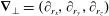 $\unicode[STIX]{x1D735}_{\bot }=(\unicode[STIX]{x2202}_{r_{x}},\unicode[STIX]{x2202}_{r_{y}},\unicode[STIX]{x2202}_{r_{z}})$
and
$\unicode[STIX]{x1D735}_{\bot }=(\unicode[STIX]{x2202}_{r_{x}},\unicode[STIX]{x2202}_{r_{y}},\unicode[STIX]{x2202}_{r_{z}})$
and
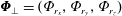 $\unicode[STIX]{x1D731}_{\bot }=(\unicode[STIX]{x1D6F7}_{r_{x}},\unicode[STIX]{x1D6F7}_{r_{y}},\unicode[STIX]{x1D6F7}_{r_{z}})$
. (b) In-plane transport velocity
$\unicode[STIX]{x1D731}_{\bot }=(\unicode[STIX]{x1D6F7}_{r_{x}},\unicode[STIX]{x1D6F7}_{r_{y}},\unicode[STIX]{x1D6F7}_{r_{z}})$
. (b) In-plane transport velocity
 $\boldsymbol{w}_{\Vert }=(w_{X},w_{Y})$
as vectors, equation (2.15) and effective net production in the plane
$\boldsymbol{w}_{\Vert }=(w_{X},w_{Y})$
as vectors, equation (2.15) and effective net production in the plane
 ${\mathcal{M}}$
, equation (4.3), as coloured contour. The yellow symbols denote the images of the bubble separatrix, see text and figure 7. (c) Same as (a) with the in-plane velocity magnified in the region
${\mathcal{M}}$
, equation (4.3), as coloured contour. The yellow symbols denote the images of the bubble separatrix, see text and figure 7. (c) Same as (a) with the in-plane velocity magnified in the region
 ${\mathcal{D}}_{II}^{\Vert }$
, see text. (d) Normal component of the in-plane transport contribution
${\mathcal{D}}_{II}^{\Vert }$
, see text. (d) Normal component of the in-plane transport contribution
 $\boldsymbol{w}_{\Vert }1/2\langle |\unicode[STIX]{x1D6FF}\boldsymbol{u}|^{2}\rangle$
to the flux (vectors) shown on the bubble separatrix. Coloured contour shows
$\boldsymbol{w}_{\Vert }1/2\langle |\unicode[STIX]{x1D6FF}\boldsymbol{u}|^{2}\rangle$
to the flux (vectors) shown on the bubble separatrix. Coloured contour shows
 $\tilde{{\mathcal{M}}}$
, equation (4.5).
$\tilde{{\mathcal{M}}}$
, equation (4.5).
Following the standard interpretation of substantial derivatives, equation (4.3) is interpreted by saying that the structure function is advected along the trajectories of the field
 $\boldsymbol{w}_{\Vert }$
and changes its magnitude due to the source term on the right-hand side. Overall, the structure function is advected toward decreasing mid-point distance from the lower wall
$\boldsymbol{w}_{\Vert }$
and changes its magnitude due to the source term on the right-hand side. Overall, the structure function is advected toward decreasing mid-point distance from the lower wall
 $Y$
and toward decreasing wall-normal separation
$Y$
and toward decreasing wall-normal separation
 $r_{y}$
, indicating that most of the flux
$r_{y}$
, indicating that most of the flux
 $\unicode[STIX]{x1D731}_{\Vert }$
taking place in the same region is associated with transport. Focusing on the shear layer, coincident with the two elongated regions where
$\unicode[STIX]{x1D731}_{\Vert }$
taking place in the same region is associated with transport. Focusing on the shear layer, coincident with the two elongated regions where
 ${\mathcal{M}}$
is intense just above the two images of the separatrix, the advection velocity is directed almost parallel to the images of the separatrix, towards smaller wall-normal mid-point distances
${\mathcal{M}}$
is intense just above the two images of the separatrix, the advection velocity is directed almost parallel to the images of the separatrix, towards smaller wall-normal mid-point distances
 $Y$
and smaller wall-normal separations
$Y$
and smaller wall-normal separations
 $r_{y}$
. A bias is added to this gross trend, such that the
$r_{y}$
. A bias is added to this gross trend, such that the
 $\boldsymbol{w}_{\Vert }$
velocity is slightly more inclined downwards than the local tangent to the separatrix. This means that the structure function, advected by the velocity field, crosses the separatrix from region
$\boldsymbol{w}_{\Vert }$
velocity is slightly more inclined downwards than the local tangent to the separatrix. This means that the structure function, advected by the velocity field, crosses the separatrix from region
 ${\mathcal{D}}_{OO}$
above to enter region
${\mathcal{D}}_{OO}$
above to enter region
 ${\mathcal{D}}_{IO}$
(left half of the plot, crossing the triangles) or
${\mathcal{D}}_{IO}$
(left half of the plot, crossing the triangles) or
 ${\mathcal{D}}_{OI}$
(right half of the plot, crossing the circles). In other words, one of the two points (e.g.
${\mathcal{D}}_{OI}$
(right half of the plot, crossing the circles). In other words, one of the two points (e.g.
 $\tilde{\boldsymbol{x}}$
as concerning the left part) is entering the recirculation bubble, while the other one remains outside. Following the advection velocity, the former point eventually enters the bubble. When this happens the point in phase space crosses the second image of the separatrix (the circles) leaving region
$\tilde{\boldsymbol{x}}$
as concerning the left part) is entering the recirculation bubble, while the other one remains outside. Following the advection velocity, the former point eventually enters the bubble. When this happens the point in phase space crosses the second image of the separatrix (the circles) leaving region
 ${\mathcal{D}}_{IO}$
to enter
${\mathcal{D}}_{IO}$
to enter
 ${\mathcal{D}}_{II}$
. Just before the second image of the separatrix is crossed (point
${\mathcal{D}}_{II}$
. Just before the second image of the separatrix is crossed (point
 $\boldsymbol{x}$
still in the shear layer) a positive value of
$\boldsymbol{x}$
still in the shear layer) a positive value of
 ${\mathcal{M}}$
is encountered, implying that the intensity of the structure function increases while advection by
${\mathcal{M}}$
is encountered, implying that the intensity of the structure function increases while advection by
 $\boldsymbol{w}_{\Vert }$
occurs.
$\boldsymbol{w}_{\Vert }$
occurs.
Equation (4.3) can be recast in conservative form as
 $$\begin{eqnarray}\displaystyle \unicode[STIX]{x1D735}_{\Vert }\boldsymbol{\cdot }\left(\boldsymbol{w}_{\Vert }{\textstyle \frac{1}{2}}\langle |\unicode[STIX]{x1D6FF}\boldsymbol{u}|^{2}\rangle \right)=\tilde{{\mathcal{M}}}={\mathcal{M}}+{\textstyle \frac{1}{2}}\langle |\unicode[STIX]{x1D6FF}\boldsymbol{u}|^{2}\rangle \unicode[STIX]{x1D735}_{\Vert }\boldsymbol{\cdot }\boldsymbol{w}_{\Vert }. & & \displaystyle\end{eqnarray}$$
This equation can be integrated in the domain
 $D_{II}^{\Vert }$
, defined as the trace of the phase space domain
$D_{II}^{\Vert }$
, defined as the trace of the phase space domain
 ${\mathcal{D}}_{II}$
in the considered
${\mathcal{D}}_{II}$
in the considered
 $(Y,r_{y})$
-plane, to yield
$(Y,r_{y})$
-plane, to yield
 $$\begin{eqnarray}\displaystyle \int _{\unicode[STIX]{x2202}{\mathcal{D}}_{II}^{\Vert }}\boldsymbol{w}_{\Vert }\frac{1}{2}\langle |\unicode[STIX]{x1D6FF}\boldsymbol{u}|^{2}\rangle \boldsymbol{\cdot }\boldsymbol{n}_{\Vert }\,\text{d}l_{\Vert }=\int _{{\mathcal{D}}_{II}^{\Vert }}\tilde{{\mathcal{M}}}\,\text{d}S_{\Vert }, & & \displaystyle\end{eqnarray}$$
where
 $\boldsymbol{n}_{\Vert }$
is the outward normal. Panel (c) of figure 7 provides the isolines of
$\boldsymbol{n}_{\Vert }$
is the outward normal. Panel (c) of figure 7 provides the isolines of
 $\tilde{{\mathcal{M}}}$
and shows the normal component of the advective flux on the boundary of region
$\tilde{{\mathcal{M}}}$
and shows the normal component of the advective flux on the boundary of region
 ${\mathcal{D}}_{II}^{\Vert }$
shown as the vector field
${\mathcal{D}}_{II}^{\Vert }$
shown as the vector field
 $\boldsymbol{n}_{\Vert }\boldsymbol{\cdot }\boldsymbol{w}_{\Vert }1/2\langle |\unicode[STIX]{x1D6FF}\boldsymbol{u}|^{2}\rangle \boldsymbol{n}_{\Vert }$
. The structure function is advected inside the bubble, with the corresponding flux balancing the negative value of the relevant source term
$\boldsymbol{n}_{\Vert }\boldsymbol{\cdot }\boldsymbol{w}_{\Vert }1/2\langle |\unicode[STIX]{x1D6FF}\boldsymbol{u}|^{2}\rangle \boldsymbol{n}_{\Vert }$
. The structure function is advected inside the bubble, with the corresponding flux balancing the negative value of the relevant source term
 $\tilde{{\mathcal{M}}}$
.
$\tilde{{\mathcal{M}}}$
.
4.3 Sub-manifold
$(Y,r_{x})$

Figure 9 addresses the
 $(Y,r_{x})_{X^{0}=5.8,r_{y}=0,r_{x}=0.4}$
-plane, which also crosses the maximum of net production. The interpretation of the different panels should now be familiar from the discussion of the previous plane. Panel (a) shows the in-plane component of the flux as vectors,
$(Y,r_{x})_{X^{0}=5.8,r_{y}=0,r_{x}=0.4}$
-plane, which also crosses the maximum of net production. The interpretation of the different panels should now be familiar from the discussion of the previous plane. Panel (a) shows the in-plane component of the flux as vectors,
 $\unicode[STIX]{x1D731}_{\Vert }=(\unicode[STIX]{x1D6F7}_{Y},\unicode[STIX]{x1D6F7}_{r_{x}})$
, the source term of (4.1) as colour contours, where now
$\unicode[STIX]{x1D731}_{\Vert }=(\unicode[STIX]{x1D6F7}_{Y},\unicode[STIX]{x1D6F7}_{r_{x}})$
, the source term of (4.1) as colour contours, where now
 $\unicode[STIX]{x1D731}_{\bot }=(\unicode[STIX]{x1D6F7}_{X},\unicode[STIX]{x1D6F7}_{r_{y}},\unicode[STIX]{x1D6F7}_{r_{z}})$
, and the structure function as solid isolines. The two images of the separatrix in this plane, curves of the form
$\unicode[STIX]{x1D731}_{\bot }=(\unicode[STIX]{x1D6F7}_{X},\unicode[STIX]{x1D6F7}_{r_{y}},\unicode[STIX]{x1D6F7}_{r_{z}})$
, and the structure function as solid isolines. The two images of the separatrix in this plane, curves of the form
 $Y=g_{b}(X^{0}\pm r_{x}/2)\mp r_{y}^{0}/2$
, are represented by the yellow symbols with the same meaning discussed previously. The in-plane flux is significant in regions
$Y=g_{b}(X^{0}\pm r_{x}/2)\mp r_{y}^{0}/2$
, are represented by the yellow symbols with the same meaning discussed previously. The in-plane flux is significant in regions
 ${\mathcal{D}}_{IO}^{\Vert }$
and
${\mathcal{D}}_{IO}^{\Vert }$
and
 ${\mathcal{D}}_{OI}^{\Vert }$
(one point is in the shear layer and the second inside the bubble) and is directed towards larger streamwise separations,
${\mathcal{D}}_{OI}^{\Vert }$
(one point is in the shear layer and the second inside the bubble) and is directed towards larger streamwise separations,
 $|r_{x}|$
. This trend is similar in region
$|r_{x}|$
. This trend is similar in region
 ${\mathcal{D}}_{II}^{\Vert }$
(both points inside the bubble). The in-plane transport velocity
${\mathcal{D}}_{II}^{\Vert }$
(both points inside the bubble). The in-plane transport velocity
 $\boldsymbol{w}_{\Vert }=(w_{Y},w_{r_{x}})$
shown in panel (b) together with the colour isolines of
$\boldsymbol{w}_{\Vert }=(w_{Y},w_{r_{x}})$
shown in panel (b) together with the colour isolines of
 ${\mathcal{M}}$
, equation (4.4), confirms the same picture and shows the advection of the structure function towards increasing streamwise separations in the regions
${\mathcal{M}}$
, equation (4.4), confirms the same picture and shows the advection of the structure function towards increasing streamwise separations in the regions
 ${\mathcal{D}}_{IO}^{\Vert }$
and
${\mathcal{D}}_{IO}^{\Vert }$
and
 ${\mathcal{D}}_{OI}^{\Vert }$
. Therefore, the separation vector
${\mathcal{D}}_{OI}^{\Vert }$
. Therefore, the separation vector
 $\boldsymbol{r}$
is stretched in the streamwise direction along the trajectory in phase space, at an almost constant mid-point distance from the lower wall. This effect corresponds to
$\boldsymbol{r}$
is stretched in the streamwise direction along the trajectory in phase space, at an almost constant mid-point distance from the lower wall. This effect corresponds to
 $\dot{\ell }>0$
in the language adopted in the last paragraphs of § 2.2. Additional features are observed inside
$\dot{\ell }>0$
in the language adopted in the last paragraphs of § 2.2. Additional features are observed inside
 ${\mathcal{D}}_{II}^{\Vert }$
, where the advection velocity reverses close to the wall images. The vectors are magnified in panel (c) for a better view. In this region, the structure function is transported in a recirculating way. It is advected to smaller streamwise scales close to the wall, then away from the wall towards the separatrix and finally towards larger streamwise separations to match the behaviour in the regions above. In Lagrangian terms, the process would correspond to stretching
${\mathcal{D}}_{II}^{\Vert }$
, where the advection velocity reverses close to the wall images. The vectors are magnified in panel (c) for a better view. In this region, the structure function is transported in a recirculating way. It is advected to smaller streamwise scales close to the wall, then away from the wall towards the separatrix and finally towards larger streamwise separations to match the behaviour in the regions above. In Lagrangian terms, the process would correspond to stretching
 $\dot{\ell }>0$
in the higher part of the (physical) recirculating bubble and compressing
$\dot{\ell }>0$
in the higher part of the (physical) recirculating bubble and compressing
 $\dot{\ell }<0$
in the lower part. Panel (d) shows the normal component of the advection flux
$\dot{\ell }<0$
in the lower part. Panel (d) shows the normal component of the advection flux
 $\boldsymbol{w}_{\Vert }1/2\langle |\unicode[STIX]{x1D6FF}\boldsymbol{u}|^{2}\rangle$
across the boundaries of region
$\boldsymbol{w}_{\Vert }1/2\langle |\unicode[STIX]{x1D6FF}\boldsymbol{u}|^{2}\rangle$
across the boundaries of region
 ${\mathcal{D}}_{II}^{\Vert }$
. The flux enters the bubble to balance the relevant source term
${\mathcal{D}}_{II}^{\Vert }$
. The flux enters the bubble to balance the relevant source term
 $\tilde{{\mathcal{M}}}$
.
$\tilde{{\mathcal{M}}}$
.
It is instructive to consider the same kind of plane, now at a positive wall-normal separation
 $r_{y}^{0}=0.12$
, figure 10. This choice is motivated by the fact that flux vectors in figure 7 converge into a sink for this specific separation. The point
$r_{y}^{0}=0.12$
, figure 10. This choice is motivated by the fact that flux vectors in figure 7 converge into a sink for this specific separation. The point
 $\tilde{\boldsymbol{x}}$
is now further from the lower channel wall than
$\tilde{\boldsymbol{x}}$
is now further from the lower channel wall than
 $\boldsymbol{x}$
(
$\boldsymbol{x}$
(
 ${\tilde{y}}-y=r_{y}>0$
), a configuration that enhances the role of the shear. In panel (a), a substantial flux
${\tilde{y}}-y=r_{y}>0$
), a configuration that enhances the role of the shear. In panel (a), a substantial flux
 $\unicode[STIX]{x1D731}_{\Vert }$
is found in the region of intense production corresponding to the shear layer (region
$\unicode[STIX]{x1D731}_{\Vert }$
is found in the region of intense production corresponding to the shear layer (region
 ${\mathcal{D}}_{OO}^{\Vert }$
, just above the yellow symbols). The flux is systematically directed from negative streamwise separations (
${\mathcal{D}}_{OO}^{\Vert }$
, just above the yellow symbols). The flux is systematically directed from negative streamwise separations (
 $r_{x}<0$
) towards positive ones (
$r_{x}<0$
) towards positive ones (
 $r_{x}>0$
), i.e. the flux vectors are oriented from left to right. The flux is mostly inertial, as seen in panel (b) which shows the corresponding transport velocity
$r_{x}>0$
), i.e. the flux vectors are oriented from left to right. The flux is mostly inertial, as seen in panel (b) which shows the corresponding transport velocity
 $\boldsymbol{w}_{\Vert }$
. One may imagine to reconstruct the kinematics of this transport process. Following the trajectories of
$\boldsymbol{w}_{\Vert }$
. One may imagine to reconstruct the kinematics of this transport process. Following the trajectories of
 $\boldsymbol{w}_{\Vert }$
, the motion is at more or less constant
$\boldsymbol{w}_{\Vert }$
, the motion is at more or less constant
 $Y$
, that is the mid-point distance from the wall remains almost constant. Starting from the left side where
$Y$
, that is the mid-point distance from the wall remains almost constant. Starting from the left side where
 $r_{x}<0$
,
$r_{x}<0$
,
 $r_{x}$
progressively increases along the trajectory to eventually become increasingly positive. Keeping in mind that
$r_{x}$
progressively increases along the trajectory to eventually become increasingly positive. Keeping in mind that
 $r_{y}^{0}>0$
in this plane, the processes can be interpreted as a sequence where the separation vector follows kinematics described by
$r_{y}^{0}>0$
in this plane, the processes can be interpreted as a sequence where the separation vector follows kinematics described by
 $r_{x}=r_{x}[s(t)]$
,
$r_{x}=r_{x}[s(t)]$
,
 $r_{y}=r_{y}^{0}$
,
$r_{y}=r_{y}^{0}$
,
 $r_{z}=r_{z}^{0}$
, with
$r_{z}=r_{z}^{0}$
, with
 $s(t)$
the arc length along the phase space trajectory increasing with time along the advection,
$s(t)$
the arc length along the phase space trajectory increasing with time along the advection,
 ${\dot{s}}=|\boldsymbol{w}_{\Vert }|$
, with
${\dot{s}}=|\boldsymbol{w}_{\Vert }|$
, with
 $\text{d}r_{x}/\text{d}s>0$
as apparent from the plot. This is consistent with a rotation of the separation vector induced by the shear, see § 2.2. It is however important to consider that the separation vector components outside the plane (
$\text{d}r_{x}/\text{d}s>0$
as apparent from the plot. This is consistent with a rotation of the separation vector induced by the shear, see § 2.2. It is however important to consider that the separation vector components outside the plane (
 $r_{y}$
and
$r_{y}$
and
 $r_{z}$
) are frozen in the present plane.
$r_{z}$
) are frozen in the present plane.
4.4 Sub-manifold
$(X,r_{x})$

The downstream behaviour is addressed in figure 11 that shows the
 $(X,r_{x})_{Y^{0}=0.45,r_{y}^{0}=0,r_{z}^{0}=0.4}$
-plane. Outside the bubble (
$(X,r_{x})_{Y^{0}=0.45,r_{y}^{0}=0,r_{z}^{0}=0.4}$
-plane. Outside the bubble (
 ${\mathcal{D}}_{OO}^{\Vert }$
region), the in-plane flux
${\mathcal{D}}_{OO}^{\Vert }$
region), the in-plane flux
 $\unicode[STIX]{x1D731}_{\Vert }=(\unicode[STIX]{x1D6F7}_{X},\unicode[STIX]{x1D6F7}_{r_{x}})$
is directed in the streamwise direction
$\unicode[STIX]{x1D731}_{\Vert }=(\unicode[STIX]{x1D6F7}_{X},\unicode[STIX]{x1D6F7}_{r_{x}})$
is directed in the streamwise direction
 $X$
, with a small component towards larger streamwise scales
$X$
, with a small component towards larger streamwise scales
 $|r_{x}|$
, see panel (a). The physical origin of this flux is basically convective, as shown by the transport velocity field
$|r_{x}|$
, see panel (a). The physical origin of this flux is basically convective, as shown by the transport velocity field
 $\boldsymbol{w}_{\Vert }$
of panel (b). The
$\boldsymbol{w}_{\Vert }$
of panel (b). The
 $r_{x}$
component of the transport velocity becomes dominant in regions
$r_{x}$
component of the transport velocity becomes dominant in regions
 ${\mathcal{D}}_{IO/OI}^{\Vert }$
and in
${\mathcal{D}}_{IO/OI}^{\Vert }$
and in
 ${\mathcal{D}}_{II}^{\Vert }$
, see panel (c) where the vectors in the latter region are magnified for better readability. The Lagrangian interpretation corresponds to the stretching of the separation vector,
${\mathcal{D}}_{II}^{\Vert }$
, see panel (c) where the vectors in the latter region are magnified for better readability. The Lagrangian interpretation corresponds to the stretching of the separation vector,
 $\dot{\ell }>0$
, implying that the structure function is advected at larger scales in the streamwise direction. A peculiar aspect of this plane is that the convective flux
$\dot{\ell }>0$
, implying that the structure function is advected at larger scales in the streamwise direction. A peculiar aspect of this plane is that the convective flux
 $\boldsymbol{w}_{\Vert }1/2\langle |\unicode[STIX]{x1D6FF}\boldsymbol{u}|^{2}\rangle$
is directed outside the bubble region feeding the neighbouring regions,
$\boldsymbol{w}_{\Vert }1/2\langle |\unicode[STIX]{x1D6FF}\boldsymbol{u}|^{2}\rangle$
is directed outside the bubble region feeding the neighbouring regions,
 ${\mathcal{D}}_{IO/OI}^{\Vert }$
, a feature already apparent from the total in-plane flux
${\mathcal{D}}_{IO/OI}^{\Vert }$
, a feature already apparent from the total in-plane flux
 $\unicode[STIX]{x1D731}_{\Vert }$
of panel (a).
$\unicode[STIX]{x1D731}_{\Vert }$
of panel (a).
4.5 Sub-manifold
$(X,Y)$

Finally, figure 12 examines the dynamics of the combined shear layer/separation bubble system in the
 $(X,Y)$
-plane at fixed
$(X,Y)$
-plane at fixed
 $r_{x}^{0}=0.45,\,r_{y}^{0}=0,\,r_{z}^{0}=0.4$
. The in-plane flux
$r_{x}^{0}=0.45,\,r_{y}^{0}=0,\,r_{z}^{0}=0.4$
. The in-plane flux
 $\unicode[STIX]{x1D731}_{\Vert }=(\unicode[STIX]{x1D6F7}_{X},\unicode[STIX]{x1D6F7}_{Y})$
is particularly strong in the shear layer, above the yellow circles (region
$\unicode[STIX]{x1D731}_{\Vert }=(\unicode[STIX]{x1D6F7}_{X},\unicode[STIX]{x1D6F7}_{Y})$
is particularly strong in the shear layer, above the yellow circles (region
 ${\mathcal{D}}_{OO}^{\Vert }$
), where the intensity of net production is large (red background contours). The flux is mainly directed in the streamwise direction
${\mathcal{D}}_{OO}^{\Vert }$
), where the intensity of net production is large (red background contours). The flux is mainly directed in the streamwise direction
 $X$
and roughly follows the profile of the separatrix (circles), bends downwards, and encounters a region of negative net production (blue). The in-plane velocity
$X$
and roughly follows the profile of the separatrix (circles), bends downwards, and encounters a region of negative net production (blue). The in-plane velocity
 $\boldsymbol{w}_{\Vert }$
, panel (b), confirms a significant convective effect transporting the structure function downstream. The magnified vectors inside the bubble, region
$\boldsymbol{w}_{\Vert }$
, panel (b), confirms a significant convective effect transporting the structure function downstream. The magnified vectors inside the bubble, region
 ${\mathcal{D}}_{II}^{\Vert }$
, panel (c), provide evidence of the recirculating advection of the structure function inside the bubble where the source term is mostly negative (blue region below the yellow triangles). In this plane, where the separation vector is constant, the mid-point where the structure function is evaluated is advected along a recirculating path. Along a closed phase space streamline, panel (c), the structure function is attenuated in intensity in the lower part of the path, where the advection is upstream (negative
${\mathcal{D}}_{II}^{\Vert }$
, panel (c), provide evidence of the recirculating advection of the structure function inside the bubble where the source term is mostly negative (blue region below the yellow triangles). In this plane, where the separation vector is constant, the mid-point where the structure function is evaluated is advected along a recirculating path. Along a closed phase space streamline, panel (c), the structure function is attenuated in intensity in the lower part of the path, where the advection is upstream (negative
 $X$
-direction) to regain intensity in the upper part of the circuit, just below the separatrix. Panel (d) shows the normal component of the advection flux
$X$
-direction) to regain intensity in the upper part of the circuit, just below the separatrix. Panel (d) shows the normal component of the advection flux
 $\boldsymbol{w}_{\Vert }1/2\langle |\unicode[STIX]{x1D6FF}\boldsymbol{u}|^{2}\rangle$
across the boundaries of region
$\boldsymbol{w}_{\Vert }1/2\langle |\unicode[STIX]{x1D6FF}\boldsymbol{u}|^{2}\rangle$
across the boundaries of region
 ${\mathcal{D}}_{II}^{\Vert }$
. Clearly, the inward fluxes prevail, confirming the dissipative features of the (physical) recirculating bubble.
${\mathcal{D}}_{II}^{\Vert }$
. Clearly, the inward fluxes prevail, confirming the dissipative features of the (physical) recirculating bubble.
In the above statistical analysis of the shear layer/recirculation bubble dynamics based on the GKE, we find that the bubble exchanges fluxes of structure function intensity with the surroundings, the shear layer being identified as the corresponding physical source. The exchange is mostly associated with convection, as shown by the normal component of the advective flux. The convective flux exchanged between the neighbouring regions
 ${\mathcal{D}}_{OO}$
,
${\mathcal{D}}_{OO}$
,
 ${\mathcal{D}}_{IO/OI}$
and
${\mathcal{D}}_{IO/OI}$
and
 ${\mathcal{D}}_{II}$
can easily be shown to be a genuine effect of fluctuations. Indeed, the transport velocity
${\mathcal{D}}_{II}$
can easily be shown to be a genuine effect of fluctuations. Indeed, the transport velocity
 $\boldsymbol{w}_{6}$
, equations (2.14) and (2.15), follows from two distinct contributions and can be decomposed as
$\boldsymbol{w}_{6}$
, equations (2.14) and (2.15), follows from two distinct contributions and can be decomposed as
 $$\begin{eqnarray}\displaystyle \left.\begin{array}{@{}l@{}}\displaystyle \boldsymbol{w}_{\boldsymbol{X}}=\frac{\langle \boldsymbol{U}^{\ast }|\unicode[STIX]{x1D6FF}\boldsymbol{u}|^{2}\rangle }{\langle |\unicode[STIX]{x1D6FF}\boldsymbol{u}|^{2}\rangle }+\frac{\langle \boldsymbol{u}^{\ast }|\unicode[STIX]{x1D6FF}\boldsymbol{u}|^{2}\rangle }{\langle |\unicode[STIX]{x1D6FF}\boldsymbol{u}|^{2}\rangle }=\boldsymbol{w}_{\boldsymbol{X}}^{M}+\boldsymbol{w}_{\boldsymbol{ X}}^{f}\\[12.0pt] \displaystyle \boldsymbol{w}_{\boldsymbol{r}}=\frac{\langle \unicode[STIX]{x1D6FF}\boldsymbol{U}|\unicode[STIX]{x1D6FF}\boldsymbol{u}|^{2}\rangle }{\langle |\unicode[STIX]{x1D6FF}\boldsymbol{u}|^{2}\rangle }+\frac{\langle \unicode[STIX]{x1D6FF}\boldsymbol{u}|\unicode[STIX]{x1D6FF}\boldsymbol{u}|^{2}\rangle }{\langle |\unicode[STIX]{x1D6FF}\boldsymbol{u}|^{2}\rangle }=\boldsymbol{w}_{\boldsymbol{r}}^{M}+\boldsymbol{w}_{\boldsymbol{ r}}^{f},\end{array}\right\} & & \displaystyle\end{eqnarray}$$
where the superscripts
 $M$
and
$M$
and
 $f$
stand for mean, to recall the advection due to the mean flow
$f$
stand for mean, to recall the advection due to the mean flow
 $\boldsymbol{U}$
, and for fluctuation, to remind the advection of the turbulent fluctuations
$\boldsymbol{U}$
, and for fluctuation, to remind the advection of the turbulent fluctuations
 $\boldsymbol{u}$
, respectively.
$\boldsymbol{u}$
, respectively.
 $\boldsymbol{U}^{\ast }=(\boldsymbol{U}(\tilde{\boldsymbol{x}})+\boldsymbol{U}(\boldsymbol{x}))/2$
and
$\boldsymbol{U}^{\ast }=(\boldsymbol{U}(\tilde{\boldsymbol{x}})+\boldsymbol{U}(\boldsymbol{x}))/2$
and
 $\unicode[STIX]{x1D6FF}\boldsymbol{U}=\boldsymbol{U}(\tilde{\boldsymbol{x}})-\boldsymbol{U}(\boldsymbol{x})$
are non-fluctuating quantities, hence, from (4.7),
$\unicode[STIX]{x1D6FF}\boldsymbol{U}=\boldsymbol{U}(\tilde{\boldsymbol{x}})-\boldsymbol{U}(\boldsymbol{x})$
are non-fluctuating quantities, hence, from (4.7),
 $\boldsymbol{w}_{\boldsymbol{X}}^{M}=\boldsymbol{U}^{\ast }$
and
$\boldsymbol{w}_{\boldsymbol{X}}^{M}=\boldsymbol{U}^{\ast }$
and
 $\boldsymbol{w}_{\boldsymbol{r}}^{M}=\unicode[STIX]{x1D6FF}\boldsymbol{U}$
. As a consequence, the phase space point
$\boldsymbol{w}_{\boldsymbol{r}}^{M}=\unicode[STIX]{x1D6FF}\boldsymbol{U}$
. As a consequence, the phase space point
 $(\boldsymbol{X},\boldsymbol{r})$
advected by the field
$(\boldsymbol{X},\boldsymbol{r})$
advected by the field
 $\boldsymbol{w}_{6}$
cannot be made to cross the two manifolds
$\boldsymbol{w}_{6}$
cannot be made to cross the two manifolds
 $f_{b}(\boldsymbol{X}\pm \boldsymbol{r}/2)=0$
, images of the physical separatrix in the phase space, by solely pure mean convection. The reason being that neither one of the two points
$f_{b}(\boldsymbol{X}\pm \boldsymbol{r}/2)=0$
, images of the physical separatrix in the phase space, by solely pure mean convection. The reason being that neither one of the two points
 $\tilde{\boldsymbol{x}}$
and
$\tilde{\boldsymbol{x}}$
and
 $\boldsymbol{x}$
can cross the separatrix by the sole advection of the mean flow given the definition of separatrix as streamline (of the mean flow velocity) separating the bubble region with closed streamlines from the outer field where the streamlines are open. In fact, the normal convective fluxes shown in the last panels of figures 7, 9, 11 and 12 should be interpreted as a consequence of the turbulent transport velocity
$\boldsymbol{x}$
can cross the separatrix by the sole advection of the mean flow given the definition of separatrix as streamline (of the mean flow velocity) separating the bubble region with closed streamlines from the outer field where the streamlines are open. In fact, the normal convective fluxes shown in the last panels of figures 7, 9, 11 and 12 should be interpreted as a consequence of the turbulent transport velocity
 $(\boldsymbol{w}_{\Vert }^{f}\boldsymbol{\cdot }\boldsymbol{n}_{\Vert })1/2\langle |\unicode[STIX]{x1D6FF}\boldsymbol{u}|^{2}\rangle \boldsymbol{n}_{\Vert }$
. In other words, using standard nomenclature, separatrix crossing should be associated with the so-called turbulent diffusion. This expression is traditional for single-point statistics, such as for example diffusion of turbulent kinetic energy. Here, the term is referred to a phenomenon of similar origin taking place in the advection of the two-point second-order structure function.
$(\boldsymbol{w}_{\Vert }^{f}\boldsymbol{\cdot }\boldsymbol{n}_{\Vert })1/2\langle |\unicode[STIX]{x1D6FF}\boldsymbol{u}|^{2}\rangle \boldsymbol{n}_{\Vert }$
. In other words, using standard nomenclature, separatrix crossing should be associated with the so-called turbulent diffusion. This expression is traditional for single-point statistics, such as for example diffusion of turbulent kinetic energy. Here, the term is referred to a phenomenon of similar origin taking place in the advection of the two-point second-order structure function.
5 An intuitive link with coherent structure dynamics
An intuitive illustration of the processes described so far is provided by associating the phase space dynamics described by the GKE with effects directly visualised in physical space. The phase space processes consist of advection of a given turbulent scale
 $\ell$
by a suitably defined vector field and intensification or depletion of the structure function intensity along the advection. The shear layer and its interaction with the recirculation region have been identified as features of interest. In proposing a meaningful association between phase space and physical space dynamics one should first identify an observable in physical space that could be related to the structure function. In the context of wall-bounded shear flows, scientists are familiar with the notion of the so-called coherent structures and the effects that these intermittent features have on the flow statistics. A well-known example are the quasi-streamwise vortices and low/high speed streaks that populate the near-wall region of canonical wall-bounded flows. These objects affect correlation functions, e.g. minimum of spanwise correlations and average distance between streamwise vortices. Correlations and second-order structure functions are very close relatives. It could be envisaged that production and advection of structure function intensity are related to generation and convection of some sort of coherent structures which can be identified in the regions (mid-point positions) and scales (separation vectors) that were analysed by the GKE. Relying on the widely accepted Q-criterion for coherent structure visualisation, the picture that emerges is shown in figure 13. A forest of hairpin-like vortical structures appear out of nowhere just behind the bump, at the level of the shear layer. Such structures are indeed expected there, given the observed maximum of net production.
$\ell$
by a suitably defined vector field and intensification or depletion of the structure function intensity along the advection. The shear layer and its interaction with the recirculation region have been identified as features of interest. In proposing a meaningful association between phase space and physical space dynamics one should first identify an observable in physical space that could be related to the structure function. In the context of wall-bounded shear flows, scientists are familiar with the notion of the so-called coherent structures and the effects that these intermittent features have on the flow statistics. A well-known example are the quasi-streamwise vortices and low/high speed streaks that populate the near-wall region of canonical wall-bounded flows. These objects affect correlation functions, e.g. minimum of spanwise correlations and average distance between streamwise vortices. Correlations and second-order structure functions are very close relatives. It could be envisaged that production and advection of structure function intensity are related to generation and convection of some sort of coherent structures which can be identified in the regions (mid-point positions) and scales (separation vectors) that were analysed by the GKE. Relying on the widely accepted Q-criterion for coherent structure visualisation, the picture that emerges is shown in figure 13. A forest of hairpin-like vortical structures appear out of nowhere just behind the bump, at the level of the shear layer. Such structures are indeed expected there, given the observed maximum of net production.

Figure 13. Isosurfaces of
 $Q$
coloured by instantaneous streamwise velocity for case
$Q$
coloured by instantaneous streamwise velocity for case
 $Re=2500$
. The threshold chosen is
$Re=2500$
. The threshold chosen is
 $Q_{0}=40$
and
$Q_{0}=40$
and
 $Q$
varies between
$Q$
varies between
 $Q_{min}=-900$
and
$Q_{min}=-900$
and
 $Q_{max}=3600$
. The threshold normalised with the average friction velocity
$Q_{max}=3600$
. The threshold normalised with the average friction velocity
 $\bar{u}_{\unicode[STIX]{x1D70F}}$
and the average wall unit
$\bar{u}_{\unicode[STIX]{x1D70F}}$
and the average wall unit
 $\bar{y}_{\unicode[STIX]{x1D70F}}$
is
$\bar{y}_{\unicode[STIX]{x1D70F}}$
is
 $Q_{0}=0.2(\bar{u}_{\unicode[STIX]{x1D70F}}/\bar{y}_{\unicode[STIX]{x1D70F}})^{2}$
.
$Q_{0}=0.2(\bar{u}_{\unicode[STIX]{x1D70F}}/\bar{y}_{\unicode[STIX]{x1D70F}})^{2}$
.
The vortical structures shown in the figure are coloured with the local streamwise velocity intensity, red meaning strong downstream convection, blue meaning upstream convection. It is apparent that the structures materialise at an
 $x$
-station that approximately corresponds, for this Reynolds number, to the end of the bump at
$x$
-station that approximately corresponds, for this Reynolds number, to the end of the bump at
 $x=5.8$
, matching the
$x=5.8$
, matching the
 $X^{0}$
corresponding to the maximum net production of structure function intensity. As the structures in the top part of the layer are convected downstream, they are tilted and their characteristic
$X^{0}$
corresponding to the maximum net production of structure function intensity. As the structures in the top part of the layer are convected downstream, they are tilted and their characteristic
 $r_{y}$
scale decreases and are stretched, i.e. their
$r_{y}$
scale decreases and are stretched, i.e. their
 $r_{x}$
characteristic scale increases. Part of the structures get trapped in the recirculation bubble and are then convected upstream, remaining close to the wall. Their intensity weakens and they eventually vanish as they move upstream climbing up the bump. The structures form again at the top edge of the recirculating bubble. Figure 14 provides a short sequence of successive snapshots where certain specific structures have been isolated from the surroundings to provide a better illustration. The downstream convection, streamwise stretching and clockwise rotation is apparent. The bottom part of the plots displays blue coloured structures that move upstream, shrink and disappear. The process of extracting a few selected structures may introduce a possible bias. To remove this potential bias, two animations are provided in the supplementary material in Movie1 and Movie2, available at https://doi.org/10.1017/jfm.2018.114. The first animation concerns the whole forest of hairpins shown in figure 13; the second one corresponds to the sequence extracted in figure 14. By looking at the animations the reader may be convinced of the strong link between the phase space interpretation and the coherent structure evolution.
$r_{x}$
characteristic scale increases. Part of the structures get trapped in the recirculation bubble and are then convected upstream, remaining close to the wall. Their intensity weakens and they eventually vanish as they move upstream climbing up the bump. The structures form again at the top edge of the recirculating bubble. Figure 14 provides a short sequence of successive snapshots where certain specific structures have been isolated from the surroundings to provide a better illustration. The downstream convection, streamwise stretching and clockwise rotation is apparent. The bottom part of the plots displays blue coloured structures that move upstream, shrink and disappear. The process of extracting a few selected structures may introduce a possible bias. To remove this potential bias, two animations are provided in the supplementary material in Movie1 and Movie2, available at https://doi.org/10.1017/jfm.2018.114. The first animation concerns the whole forest of hairpins shown in figure 13; the second one corresponds to the sequence extracted in figure 14. By looking at the animations the reader may be convinced of the strong link between the phase space interpretation and the coherent structure evolution.
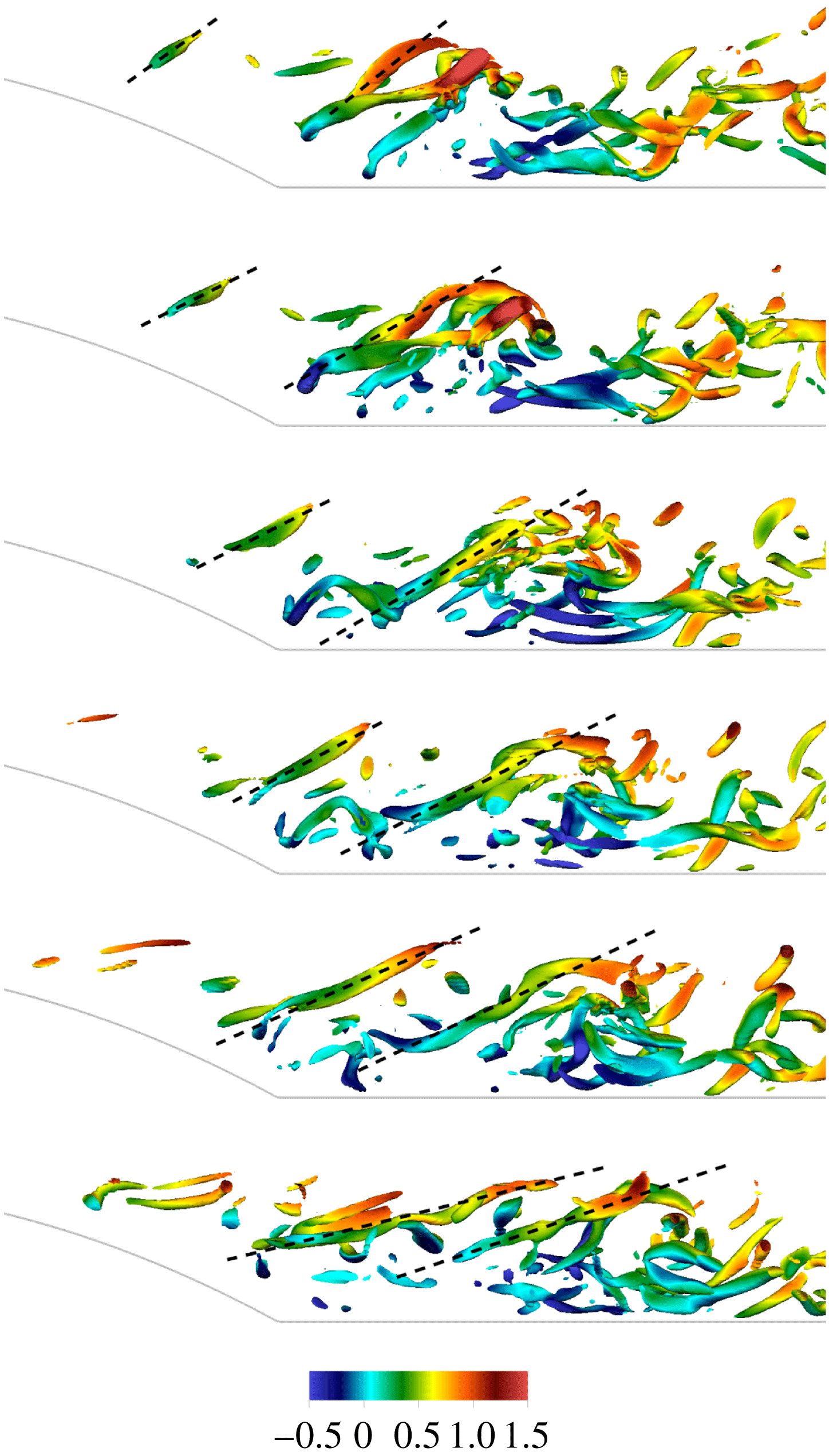
Figure 14. Isolated selection of isosurfaces of
 $Q$
coloured by instantaneous streamwise velocity in sequential snapshots for case
$Q$
coloured by instantaneous streamwise velocity in sequential snapshots for case
 $Re=2500$
. The threshold chosen is the same as in figure 13.
$Re=2500$
. The threshold chosen is the same as in figure 13.
Finally, it is worth commenting on the effect of the Reynolds number on the dynamics described so far. At
 $Re=10\,000$
, the recirculation region becomes smaller, see Mollicone et al. (Reference Mollicone, Battista, Gualtieri and Casciola2017). Figure 15 shows spanwise and wall-parallel views of the instantaneous streamwise velocity in panel (a) and (b) respectively. Despite flow structures becoming smaller and more attached to the wall, the gross features are similar to those described for the smaller Reynolds number case. The maximum net production is now found at the phase space position
$Re=10\,000$
, the recirculation region becomes smaller, see Mollicone et al. (Reference Mollicone, Battista, Gualtieri and Casciola2017). Figure 15 shows spanwise and wall-parallel views of the instantaneous streamwise velocity in panel (a) and (b) respectively. Despite flow structures becoming smaller and more attached to the wall, the gross features are similar to those described for the smaller Reynolds number case. The maximum net production is now found at the phase space position
 $X^{0}=5.1$
,
$X^{0}=5.1$
,
 $Y^{0}=0.45$
,
$Y^{0}=0.45$
,
 $r_{x}^{0}=0.17$
,
$r_{x}^{0}=0.17$
,
 $r_{y}^{0}=0$
,
$r_{y}^{0}=0$
,
 $r_{z}^{0}=0.13$
.
$r_{z}^{0}=0.13$
.
Without repeating the whole analysis, figure 16 shows in-plane fluxes, advection velocities and advective flux normal to the separatrix in the
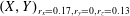 $(X,Y)_{r_{x}=0.17,r_{y}=0,r_{z}=0.13}$
- plane, to be compared with figure 12 at the smaller Reynolds number. The qualitative features are analogous, once the shorter extension of the high intensity region of the shear layer and the shorter and narrower recirculation regions are accounted for. A corresponding visualisation of the hairpin forest at
$(X,Y)_{r_{x}=0.17,r_{y}=0,r_{z}=0.13}$
- plane, to be compared with figure 12 at the smaller Reynolds number. The qualitative features are analogous, once the shorter extension of the high intensity region of the shear layer and the shorter and narrower recirculation regions are accounted for. A corresponding visualisation of the hairpin forest at
 $Re=10\,000$
is provided in figure 17, while an animation is provided in the supplementary material in Movie3.
$Re=10\,000$
is provided in figure 17, while an animation is provided in the supplementary material in Movie3.
Figure 15. Instantaneous streamwise velocity contours for
 $Re=10\,000$
. (a)
$Re=10\,000$
. (a)
 $(y,z)$
-plane at
$(y,z)$
-plane at
 $x^{0}=5.1$
; (b)
$x^{0}=5.1$
; (b)
 $(x,z)$
-plane at
$(x,z)$
-plane at
 $y^{0}=0.45$
.
$y^{0}=0.45$
.
Figure 16.
 $Re=10\,000$
,
$Re=10\,000$
,
 $(X,Y)$
-plane at
$(X,Y)$
-plane at
 $r_{x}^{0}=0.17$
,
$r_{x}^{0}=0.17$
,
 $r_{y}^{0}=0$
,
$r_{y}^{0}=0$
,
 $r_{z}^{0}=0.13$
. See caption of figure 12.
$r_{z}^{0}=0.13$
. See caption of figure 12.

Figure 17. Isosurfaces of
 $Q$
coloured by instantaneous streamwise velocity for case
$Q$
coloured by instantaneous streamwise velocity for case
 $Re=10\,000$
. The threshold chosen is
$Re=10\,000$
. The threshold chosen is
 $Q_{0}=240$
and
$Q_{0}=240$
and
 $Q$
varies between
$Q$
varies between
 $Q_{min}=-11\,000$
and
$Q_{min}=-11\,000$
and
 $Q_{max}=14\,000$
. The threshold normalised with the average friction velocity
$Q_{max}=14\,000$
. The threshold normalised with the average friction velocity
 $\bar{u}_{\unicode[STIX]{x1D70F}}$
and the average wall unit
$\bar{u}_{\unicode[STIX]{x1D70F}}$
and the average wall unit
 $\bar{y}_{\unicode[STIX]{x1D70F}}$
is
$\bar{y}_{\unicode[STIX]{x1D70F}}$
is
 $Q_{0}=0.2(\bar{u}_{\unicode[STIX]{x1D70F}}/\bar{y}_{\unicode[STIX]{x1D70F}})^{2}$
.
$Q_{0}=0.2(\bar{u}_{\unicode[STIX]{x1D70F}}/\bar{y}_{\unicode[STIX]{x1D70F}})^{2}$
.
6 Final remarks
The separated turbulent flow behind the bump is characterised by a complex pattern which can be visualised in terms of coherent vortical structures. The structures are generated in the shear layer and follow two different routes: some structures are stretched and convected downstream whilst others are trapped by the recirculation bubble where, while advected upstream in the lower part of the bubble, they eventually disappear to reform again when recirculating to the top part of the bubble. This complex behaviour calls for a detailed and quantitative description in the joint space of position and scale separation. The generalised Kolmogorov equation (GKE) has proven to be the appropriate tool to achieve this. The GKE shows how the energy content at a given separation, as measured by the second-order structure function, is advected in the five-dimensional phase space
 $(X,Y,r_{x},r_{y},r_{z})$
. Results show how the maximum of net production
$(X,Y,r_{x},r_{y},r_{z})$
. Results show how the maximum of net production
 $\unicode[STIX]{x1D6F1}_{6}-2\langle \unicode[STIX]{x1D700}^{\ast }\rangle$
occurs at specific scales in the shear layer. The fluxes appearing in the GKE transfer the produced energy to different physical regions of the flow at different scales. The fluxes which feed the recirculation bubble create a direct energy cascade in the scale separation space, providing a quantitative interpretation of the recirculating bubble as a dissipative feature of the separated flow. On the other hand, the fluxes which feed the turbulent flow downstream locally create an inverse energy cascade in the separation space, that is the fluxes move energy from smaller to the larger scales. This view is corroborated by the alternative Lagrangian interpretation of the GKE discussed in the present work. Indeed, the GKE can be recast in the structure of a transport equation in the five-dimensional space by defining a generalised transport velocity. The velocity transports the second-order structure function to different positions in space and different separations and orientations. This clearly shows how a given structure at a scale
$\unicode[STIX]{x1D6F1}_{6}-2\langle \unicode[STIX]{x1D700}^{\ast }\rangle$
occurs at specific scales in the shear layer. The fluxes appearing in the GKE transfer the produced energy to different physical regions of the flow at different scales. The fluxes which feed the recirculation bubble create a direct energy cascade in the scale separation space, providing a quantitative interpretation of the recirculating bubble as a dissipative feature of the separated flow. On the other hand, the fluxes which feed the turbulent flow downstream locally create an inverse energy cascade in the separation space, that is the fluxes move energy from smaller to the larger scales. This view is corroborated by the alternative Lagrangian interpretation of the GKE discussed in the present work. Indeed, the GKE can be recast in the structure of a transport equation in the five-dimensional space by defining a generalised transport velocity. The velocity transports the second-order structure function to different positions in space and different separations and orientations. This clearly shows how a given structure at a scale
 $\ell$
is translated, rotated, stretched and/or compressed. In conclusion, the GKE and its Lagrangian view provide the statistical signature of the coherent structures which form in the shear layer and are subsequently advected and stretched downstream or dissipated inside the recirculating bubble.
$\ell$
is translated, rotated, stretched and/or compressed. In conclusion, the GKE and its Lagrangian view provide the statistical signature of the coherent structures which form in the shear layer and are subsequently advected and stretched downstream or dissipated inside the recirculating bubble.
Acknowledgements
The research has received funding from the European Research Council under the ERC Grant Agreement no. 339446. We acknowledge PRACE for awarding us access to supercomputing resource FERMI based in Bologna, Italy through PRACE project no. 2014112647.
Supplementary movies
Supplementary movies are available at https://doi.org/10.1017/jfm.2018.114.


 Open access