


1. Introduction and main results
Preferential attachment models give a credible explanation how typical features of networks, like scale-free degree distributions and small diameter, arise naturally from the basic construction principle of reinforcement. This makes them a popular model for scale-free random graphs. Unfortunately, the mathematical analysis of preferential attachment networks is much more challenging than that of many other scale-free network models, for example the configuration model. In particular, the problem of the size of the largest subcritical connected component, solved for the configuration model by Janson [Reference Janson7], is open for all model variants of preferential attachment. The purpose of the present paper is to solve this problem for a simplified class of network models of preferential attachment type. We believe that our model, which is an inhomogeneous random graph with a suitably chosen kernel, has sufficiently many common features with the most studied models of preferential attachment networks to serve as a solvable model in this universality class. Since inhomogeneous random graphs are interesting models in their own right, see [Reference Bollobás, Janson and Riordan3], their analysis is also of independent interest.
The class of inhomogeneous random graphs is parametrised by a symmetric kernel
 \begin{equation*}\kappa \colon (0,1] \times (0,1] \rightarrow (0, \infty )\end{equation*}
and constructed such that, for each $n \in \mathbb{N}$
, the graph
$n \in \mathbb{N}$
, the graph $\mathscr{G}_n$
has vertex set
$\mathscr{G}_n$
has vertex set $V_n = \{1, \ldots , n\}$
and edge set
$V_n = \{1, \ldots , n\}$
and edge set $E_n$
containing each unordered pair of distinct vertices
$E_n$
containing each unordered pair of distinct vertices $\{i,j\}\subset V_n$
independently with probability
$\{i,j\}\subset V_n$
independently with probability
 \begin{equation*}p_{ij}^{(n)}= \frac 1n \kappa \left ( \frac {i}{n}, \frac {j}{n} \right ) \wedge 1.\end{equation*}
Our idea is now to choose the kernel $\kappa$
in such a way that the inhomogeneous random graphs mimic the behaviour of preferential attachment models. In preferential attachment models vertices arrive one-by-one and attach themselves to earlier vertices with a probability proportional to their degree. Typically degrees grow polynomially so that, for some
$\kappa$
in such a way that the inhomogeneous random graphs mimic the behaviour of preferential attachment models. In preferential attachment models vertices arrive one-by-one and attach themselves to earlier vertices with a probability proportional to their degree. Typically degrees grow polynomially so that, for some $\gamma \ge 0$
, the degree of vertex
$\gamma \ge 0$
, the degree of vertex $i$
at time
$i$
at time $j\gt i$
is of order
$j\gt i$
is of order $(j/i)^\gamma$
. For the expected degree of vertex
$(j/i)^\gamma$
. For the expected degree of vertex $j$
at its arrival time to remain bounded from zero and infinity we need that
$j$
at its arrival time to remain bounded from zero and infinity we need that $\gamma \lt 1$
and the proportionality factor in the connection probability to be of order
$\gamma \lt 1$
and the proportionality factor in the connection probability to be of order $(\!\sum_{i=1}^{j-1} (j/i)^\gamma )^{-1}\approx (1/j)$
. Hence in the preferential attachment models for vertices with index
$(\!\sum_{i=1}^{j-1} (j/i)^\gamma )^{-1}\approx (1/j)$
. Hence in the preferential attachment models for vertices with index $i\lt j$
we have connection probability
$i\lt j$
we have connection probability $p_{ij}^{_{(n)}} \approx i^{-\gamma }j^{\gamma -1}$
. To get the same connection probabilities in the inhomogeneous random graph we choose the kernel
$p_{ij}^{_{(n)}} \approx i^{-\gamma }j^{\gamma -1}$
. To get the same connection probabilities in the inhomogeneous random graph we choose the kernel
 \begin{equation*}\kappa (x, y) = \beta (x \vee y)^{\gamma - 1} (x \wedge y)^{-\gamma },\end{equation*}
where the parameter $0 \leq \gamma \lt 1$
controls the strength of the preferential attachment, and
$0 \leq \gamma \lt 1$
controls the strength of the preferential attachment, and $\beta \gt 0$
is an edge density parameter. Note that
$\beta \gt 0$
is an edge density parameter. Note that $\kappa$
is homogeneous of index
$\kappa$
is homogeneous of index $-1$
and therefore the resulting edge probability
$-1$
and therefore the resulting edge probability $p_{ij}^{_{(n)}}$
is independent of the graph size
$p_{ij}^{_{(n)}}$
is independent of the graph size $n$
. We refer to this model as the inhomogeneous random graph of preferential attachment type.
$n$
. We refer to this model as the inhomogeneous random graph of preferential attachment type.
It is easy to see that the inhomogeneous random graph of preferential attachment type has an asymptotic degree distribution which, for $\gamma \gt 0$
, is heavy-tailed with power-law exponent
$\gamma \gt 0$
, is heavy-tailed with power-law exponent $\tau =1+\frac 1\gamma$
. The analysis of a preferential attachment model in [Reference Dereich and Mörters5] can be simplified, see [Reference Mörters11] for details, and shows that the size
$\tau =1+\frac 1\gamma$
. The analysis of a preferential attachment model in [Reference Dereich and Mörters5] can be simplified, see [Reference Mörters11] for details, and shows that the size $S_n^{\mathrm{max}}$
of the largest connected component in
$S_n^{\mathrm{max}}$
of the largest connected component in $\mathscr{G}_n$
satisfies
$\mathscr{G}_n$
satisfies
 \begin{equation*}\lim _{n\to \infty } \frac {S_n^{\mathrm{max}}}{n} = \theta (\beta ) \left \{ \begin{array}{ll} \gt 0 & \text{if } \beta \gt \beta _c\ \,:\!=\, \bigg(\dfrac {1}{4}-\dfrac {\gamma }{2}\bigg) \vee 0,\\ =0 & \text{otherwise.}\\ \end{array} \right . \end{equation*}
In this paper, we are interested in the subcritical regime, i.e. we always assume that $\gamma \lt \frac 12$
and
$\gamma \lt \frac 12$
and $0\lt \beta \lt \beta _c$
. In this case, all component sizes are of smaller order than
$0\lt \beta \lt \beta _c$
. In this case, all component sizes are of smaller order than $n$
. Our first result identifies the component sizes of vertices in a moving observation window. We say that vertex
$n$
. Our first result identifies the component sizes of vertices in a moving observation window. We say that vertex $o_n\in V_n$
is typical if
$o_n\in V_n$
is typical if $\frac {o_n}n \to u$
for some
$\frac {o_n}n \to u$
for some $u\gt 0$
and the behaviour of early typical vertices refers to features of
$u\gt 0$
and the behaviour of early typical vertices refers to features of $\mathscr{G}_n$
rooted in vertex
$\mathscr{G}_n$
rooted in vertex $o_n$
that hold asymptotically as
$o_n$
that hold asymptotically as $u\downarrow 0$
.
$u\downarrow 0$
.
Theorem 1 (Early typical vertices). Let $S_n(i)$
be the size of the connected component of vertex
$S_n(i)$
be the size of the connected component of vertex $i\in V_n$
in the inhomogeneous random graph of preferential attachment type in the subcritical regime. If
$i\in V_n$
in the inhomogeneous random graph of preferential attachment type in the subcritical regime. If $o_n\in V_n$
is such that
$o_n\in V_n$
is such that $\frac {o_n}n\to u\in (0,1]$
, then
$\frac {o_n}n\to u\in (0,1]$
, then
 \begin{equation*} \lim _{u \downarrow 0} \lim _{n \rightarrow \infty } \mathbb{P}\left ( S_n(o_n) \geq u^{-\rho _-}x \right )= \mathbb{P} \left ( Y\geq x \right)\!,\end{equation*}
for all $x\gt 0$
, where
$x\gt 0$
, where
 \begin{equation*}\rho _{\pm } = \frac{1}{2} \pm \sqrt {(\gamma -\tfrac {1}{2})^2+\beta (2\gamma -1)}.\end{equation*}
and $Y$
is a positive random variable satisfying
$Y$
is a positive random variable satisfying
 \begin{equation*}\mathbb{P}\left ( Y \geq x \right ) = x^{-(\rho _+/\rho _-) + o(1)} \text{ as $x\to \infty $.}\end{equation*}
Our second theorem identifies the the size of the component of untypically early vertices. Here a vertex $o_n\in V_n$
is called untypically early if
$o_n\in V_n$
is called untypically early if $\frac {o_n}n \to 0$
.
$\frac {o_n}n \to 0$
.
Theorem 2 (Untypically early vertices). Let $o_n\in V_n$
be such that
$o_n\in V_n$
be such that
 \begin{equation*} {o_n\to \infty } \text{ and } { \frac {o_n}{n} \to 0}.\end{equation*}
Denoting by $S_n(o_n)$
the size of the component of
$S_n(o_n)$
the size of the component of $o_n$
in
$o_n$
in $\mathscr{G}_n$
, then for any
$\mathscr{G}_n$
, then for any $\epsilon \gt 0$
we have
$\epsilon \gt 0$
we have
 \begin{equation*} {\lim _{n \rightarrow \infty } \mathbb{P}\left ( S_n(o_n) \geq (n/o_n)^{\rho _-{-}\epsilon } \right )= 1}.\end{equation*}
The idea behind this result is to exploit a self-similarity feature of graphs of preferential attachment type and leverage Theorem1. Loosely speaking, we find for fixed small $u\gt 0$
a positive integer
$u\gt 0$
a positive integer $k$
with
$k$
with $o_n\approx u^kn$
. Then
$o_n\approx u^kn$
. Then $o_n$
is early typical in the graph
$o_n$
is early typical in the graph $\mathscr{G}_{u^{k-1}n}$
and by Theorem1 we get a connected component with size of order
$\mathscr{G}_{u^{k-1}n}$
and by Theorem1 we get a connected component with size of order $u^{-\rho _-}$
. Many vertices in this component are themselves early typical in
$u^{-\rho _-}$
. Many vertices in this component are themselves early typical in $\mathscr{G}_{u^{k-2}n}$
and we can use Theorem1 again, getting a component with size of order
$\mathscr{G}_{u^{k-2}n}$
and we can use Theorem1 again, getting a component with size of order $u^{-2\rho _-}$
. Continuing the procedure altogether
$u^{-2\rho _-}$
. Continuing the procedure altogether $k$
times we build a component of size
$k$
times we build a component of size $u^{-k\rho _-}\approx (n/o_n)^{\rho _-}$
in
$u^{-k\rho _-}\approx (n/o_n)^{\rho _-}$
in $\mathscr{G}_{n}$
.
$\mathscr{G}_{n}$
.
Theorem 2 gives a lower bound on the size of the largest component. As it describes the size of the components of the most powerful vertices in $\mathscr{G}_n$
it is plausible that this result also gives the right order of the largest component. Our main result confirms this. It is the first result in the mathematical literature identifying the size of the largest subcritical component up to polynomial order for a random graph model of preferential attachment type.
$\mathscr{G}_n$
it is plausible that this result also gives the right order of the largest component. Our main result confirms this. It is the first result in the mathematical literature identifying the size of the largest subcritical component up to polynomial order for a random graph model of preferential attachment type.
Theorem 3 (Largest subcritical component). Denoting by $S_n^{\mathrm{max}}$
the size of the largest component in
$S_n^{\mathrm{max}}$
the size of the largest component in $\mathscr{G}_n$
we have
$\mathscr{G}_n$
we have
 \begin{equation*}\lim _{n \rightarrow \infty } \frac {\log S_n^{\mathrm{max}}}{\log n} = \rho _{-},\end{equation*}
in probability, where
 \begin{equation*}\rho _{-} = \frac{1}{2} - \sqrt {(\tfrac {1}{2}-\gamma )^2-\beta (1-2\gamma )} \gt \gamma .\end{equation*}
Remark 4. Observe that the size of the largest component in a finite random graph is bounded from below by the maximum over all degrees. In scale-free graphs this is of polynomial order in the graph size. It is shown in [Reference Janson7] that this lower bound is sharp for configuration models and inhomogeneous random graphs with a kernel of rank one. In our model the largest degree is $n^{\gamma +o(1)}$
, whereas the largest component has size
$n^{\gamma +o(1)}$
, whereas the largest component has size $n^{\rho _-+o(1)}$
and is therefore much larger. A lower bound on the largest component larger than the maximal degree has also been found for a different preferential attachment model in [Reference Ray14], see also [Reference Banerjee, Bhamidi, van der Hofstad and Ray4] for recent further developments. As this effect is due to the self-similar nature of the graphs of preferential attachment type we conjecture that it is a universal feature of preferential attachment graphs that if the largest degree is
$n^{\rho _-+o(1)}$
and is therefore much larger. A lower bound on the largest component larger than the maximal degree has also been found for a different preferential attachment model in [Reference Ray14], see also [Reference Banerjee, Bhamidi, van der Hofstad and Ray4] for recent further developments. As this effect is due to the self-similar nature of the graphs of preferential attachment type we conjecture that it is a universal feature of preferential attachment graphs that if the largest degree is $n^{\gamma (\beta )+o(1)}$
the largest subcritical component is of size
$n^{\gamma (\beta )+o(1)}$
the largest subcritical component is of size $n^{\rho (\beta )+o(1)}$
for some
$n^{\rho (\beta )+o(1)}$
for some $\rho (\beta )\gt \gamma (\beta )$
with
$\rho (\beta )\gt \gamma (\beta )$
with $\rho (\beta )\to \frac 12$
as
$\rho (\beta )\to \frac 12$
as $\beta \uparrow \beta _c$
.
$\beta \uparrow \beta _c$
.
The remainder of the paper is organised as follows. We will not give the full proof of Theorem1 here as the argument is described in the extended abstract [Reference Mörters, Schleicher, Mailler and Wild12]. We will however give a completely self-contained proof of Theorem2 and therefore include most arguments that are needed for the proof of Theorem1. This proof of Theorem2 will be given in Section 2. Note that Theorem2 also establishes the lower bound in Theorem3 and in Section 3, we complete the proof of Theorem3 by providing an upper bound.
2. Proof of Theorem 2
For the proof of Theorem2 we embed a Galton-Watson tree into our graph. To explain the idea fix small parameters $0\lt u,b \lt 1$
. Let
$0\lt u,b \lt 1$
. Let $m=u^{k-1}n$
for some positive integer
$m=u^{k-1}n$
for some positive integer $k$
(in the following, to avoid cluttering notation, we do not make the rounding of
$k$
(in the following, to avoid cluttering notation, we do not make the rounding of $m$
to an integer explicit). We explore the neighbourhood of a vertex
$m$
to an integer explicit). We explore the neighbourhood of a vertex $o_n$
with
$o_n$
with $bum \leq o_n\leq um$
in the graph
$bum \leq o_n\leq um$
in the graph $\mathscr{G}_{m}$
. We will see below that this exploration can be coupled to a branching random walk killed upon leaving a bounded interval such that with high probability the number of particles near the right interval boundary exceeds the number
$\mathscr{G}_{m}$
. We will see below that this exploration can be coupled to a branching random walk killed upon leaving a bounded interval such that with high probability the number of particles near the right interval boundary exceeds the number $S_m(o_n)$
of vertices in the connected component of
$S_m(o_n)$
of vertices in the connected component of $o_n\in \mathscr{G}_m$
with index at least
$o_n\in \mathscr{G}_m$
with index at least $bm$
. These vertices will be the offspring of the vertex
$bm$
. These vertices will be the offspring of the vertex $o_n$
in our Galton-Watson tree. Before describing this coupling in detail we give a lower bound on the number of particles in the killed branching random walk. This result, formulated as Proposition 5, may be of independent interest.
$o_n$
in our Galton-Watson tree. Before describing this coupling in detail we give a lower bound on the number of particles in the killed branching random walk. This result, formulated as Proposition 5, may be of independent interest.
We denote by $\mathscr{V}$
the tree of Ulam-Harris labels, i.e. all finite sequences of natural numbers including the empty sequence
$\mathscr{V}$
the tree of Ulam-Harris labels, i.e. all finite sequences of natural numbers including the empty sequence $\varnothing$
, which denotes the root. Given a label
$\varnothing$
, which denotes the root. Given a label $v=(v_1,\ldots , v_n)\in \mathscr{V}\setminus \{\varnothing \}$
we denote by
$v=(v_1,\ldots , v_n)\in \mathscr{V}\setminus \{\varnothing \}$
we denote by $|v|=n$
its length, corresponding to the generation of vertex
$|v|=n$
its length, corresponding to the generation of vertex $v$
in the tree and by
$v$
in the tree and by ${v}=(v_1,\ldots , v_{n-1})$
the parent of
${v}=(v_1,\ldots , v_{n-1})$
the parent of $v$
in the tree. We attach to every label
$v$
in the tree. We attach to every label $v\in \mathscr{V}$
an independent sample
$v\in \mathscr{V}$
an independent sample $P_v$
of a point process with infinitely many points
$P_v$
of a point process with infinitely many points $P_v(1)\leq P_v(2) \leq P_v(3) \leq \ldots$
in increasing order on the real line, in our case the Poisson process with intensity measure
$P_v(1)\leq P_v(2) \leq P_v(3) \leq \ldots$
in increasing order on the real line, in our case the Poisson process with intensity measure
 \begin{equation*}\pi (dx)=\beta (e^{\gamma x} {\unicode{x1D7D9}}_{x\gt 0} + e^{(1-\gamma ) x} {\unicode{x1D7D9}}_{x\lt 0}) \, dx.\end{equation*}
We denote by
 \begin{equation*}\mathscr{T}(x)= ( V(v) \colon v \in \mathscr{V})\end{equation*}
the branching random walk started in $x\in \mathbb{R}$
, which is characterised by the position
$x\in \mathbb{R}$
, which is characterised by the position
 \begin{equation*}V(v)= x + \sum _{i=1}^{|v|} P_{(v_1,\ldots , v_{i-1})}(v_i)\end{equation*}
of the particle with label $v\in \mathscr{V}$
. When started in
$v\in \mathscr{V}$
. When started in $\log u$
we denote the underlying probability and expectation by
$\log u$
we denote the underlying probability and expectation by $\mathbb{P}_u, \mathbb{E}_u$
and denote the branching random walk by
$\mathbb{P}_u, \mathbb{E}_u$
and denote the branching random walk by $\mathscr{T}$
. The Laplace transform of the branching random walk is given by
$\mathscr{T}$
. The Laplace transform of the branching random walk is given by
 \begin{align*} \psi (t)= \mathbb{E}_1\bigg[\sum _{|v|=1}e^{-tV(v)}\bigg] = \frac {\beta }{t-\gamma }+\frac {\beta }{1-\gamma -t} \quad \text{ if $\gamma \lt t\lt 1-\gamma $,} \end{align*}
and $\psi (t)=\infty$
otherwise. The domain of
$\psi (t)=\infty$
otherwise. The domain of $\psi$
is nonempty if
$\psi$
is nonempty if $\gamma \lt \frac 12$
and there exists
$\gamma \lt \frac 12$
and there exists $t\gt 0$
with
$t\gt 0$
with $\psi (t)\lt 1$
if and only if
$\psi (t)\lt 1$
if and only if $0\lt \beta \lt \frac {1}{4}-\frac {\gamma }{2}$
, i.e. in the subcritical regime for the inhomogeneous random graph. Under this assumption there exist
$0\lt \beta \lt \frac {1}{4}-\frac {\gamma }{2}$
, i.e. in the subcritical regime for the inhomogeneous random graph. Under this assumption there exist $\rho _- \lt \rho _+$
with
$\rho _- \lt \rho _+$
with $\psi (\rho _-)=\psi (\rho _+)=1$
. We can calculate both values explicitly,
$\psi (\rho _-)=\psi (\rho _+)=1$
. We can calculate both values explicitly,
 \begin{equation*} \rho _{\pm } = \frac{1}{2} \pm \sqrt{\big(\gamma -\tfrac {1}{2}\big)^2+\beta (2\gamma -1)}. \end{equation*}
For $0\leq a\lt d$
denote by
$0\leq a\lt d$
denote by $\mathscr{T}_{a,d}(x)$
the killed branching random walk starting with a particle in location
$\mathscr{T}_{a,d}(x)$
the killed branching random walk starting with a particle in location $x$
, where all particles located outside the interval
$x$
, where all particles located outside the interval $(\!\log a, \log d]$
are killed together with their descendants. Again we omit the starting point from the notation if it is clear from the context. Note that
$(\!\log a, \log d]$
are killed together with their descendants. Again we omit the starting point from the notation if it is clear from the context. Note that $v=(v_1,\ldots ,v_n)\in \mathscr{T}_{a,d}$
means that, for all
$v=(v_1,\ldots ,v_n)\in \mathscr{T}_{a,d}$
means that, for all $0\leq i \leq n$
,
$0\leq i \leq n$
,
 \begin{equation*} \log a \lt V(v_1,\ldots ,v_i) \leq \log d.\end{equation*}
Of particular interest is $\mathscr{T}_{0,1}$
where particles with positions on the positive half-line are killed. The condition
$\mathscr{T}_{0,1}$
where particles with positions on the positive half-line are killed. The condition $\gamma \lt \frac {1}{2}$
and
$\gamma \lt \frac {1}{2}$
and $\beta \lt \frac {1}{4}-\frac {\gamma }{2}$
is necessary and sufficient for
$\beta \lt \frac {1}{4}-\frac {\gamma }{2}$
is necessary and sufficient for $\mathscr{T}_{0,1}(x)$
started at
$\mathscr{T}_{0,1}(x)$
started at $x\leq 0$
to suffer extinction in finite time almost surely, see [[Reference Shi15], Theorem 1.3].
$x\leq 0$
to suffer extinction in finite time almost surely, see [[Reference Shi15], Theorem 1.3].
For $0\leq a \leq b\lt 1$
denote by
$0\leq a \leq b\lt 1$
denote by $I(a,b)$
be the total number of surviving particles of
$I(a,b)$
be the total number of surviving particles of $\mathscr{T}_{a,1}$
located in
$\mathscr{T}_{a,1}$
located in $(\log b,0]$
. We prove a limit theorem for
$(\log b,0]$
. We prove a limit theorem for $I(0,b)$
under
$I(0,b)$
under $\mathbb{P}_u$
when
$\mathbb{P}_u$
when $u \downarrow 0$
.
$u \downarrow 0$
.
Proposition 5.
For every fixed $0\leq b\lt 1$
the random variable
$0\leq b\lt 1$
the random variable $I(0,b)$
satisfies
$I(0,b)$
satisfies
 \begin{equation*}\lim _{u \downarrow 0} \mathbb{P}_u \left ( I(0,b) \geq xu^{-\rho _-} \right ) = \mathbb{P} \left(Y\geq x \right)\!,\end{equation*}
where $Y$
is a positive random variable satisfying
$Y$
is a positive random variable satisfying
 \begin{equation} \mathbb{P}\left ( Y \geq x \right ) = x^{-(\rho _+/\rho _-) + o(1)} \text{ as $x\to \infty $.} \end{equation}
Proposition 5 will be proved in Section 2.1.
This proposition will play a crucial role when we construct the simultaneous coupling of the neighbourhoods of vertices in $\mathscr{G}_m$
. We use the projection
$\mathscr{G}_m$
. We use the projection
 \begin{align} \pi _m \colon & (\!-\infty ,0] \to \{1,\ldots ,m\}, \end{align}
defined by
 \begin{equation*}-\sum _{k=\pi _m(x)}^m \frac 1k \lt x \leq -\sum _{k=\pi _m(x)+1}^m \frac 1k\end{equation*}
to map locations on the negative half-line to vertex numbers in $\mathscr{G}_m$
. Its partial inverse is
$\mathscr{G}_m$
. Its partial inverse is
 \begin{align*} \phi _m \colon & \{1, \ldots , m\} \rightarrow (-\infty ,0], \quad i \mapsto - \sum _{j=i+1}^{m} \frac {1}{j} \; . \end{align*}
For any set $\mathcal{U}\subset \{1,\ldots , m\}$
we denote by
$\mathcal{U}\subset \{1,\ldots , m\}$
we denote by $\mathscr{F}_{\mathcal{U}}$
the
$\mathscr{F}_{\mathcal{U}}$
the $\sigma$
-algebra generated by the restriction of the random graph
$\sigma$
-algebra generated by the restriction of the random graph $\mathscr{G}_m$
to the vertex set
$\mathscr{G}_m$
to the vertex set $\mathcal{U}$
. Let
$\mathcal{U}$
. Let $\gamma \lt \rho \lt \rho _-$
.
$\gamma \lt \rho \lt \rho _-$
.
Proposition 6.
For every $0\lt b\lt 1$
there exist
$0\lt b\lt 1$
there exist $\varepsilon \gt 0$
,
$\varepsilon \gt 0$
, $a\gt 1$
and
$a\gt 1$
and $0\lt u_0\lt b$
with the property that for every
$0\lt u_0\lt b$
with the property that for every $0\lt u\lt u_0$
there exists
$0\lt u\lt u_0$
there exists $m(u)$
such that, for all
$m(u)$
such that, for all $m\ge m(u)$
and any set
$m\ge m(u)$
and any set $\mathcal{U}'\subset \{1,\ldots , um\}$
with
$\mathcal{U}'\subset \{1,\ldots , um\}$
with $|\mathcal{U}'|\leq a m^{\rho }$
and family of
$|\mathcal{U}'|\leq a m^{\rho }$
and family of $d\leq m^{\rho }$
vertices in
$d\leq m^{\rho }$
vertices in $\mathcal{U}'$
with
$\mathcal{U}'$
with
 \begin{equation*}bum\lt u_1 \lt \cdots \lt u_d \leq um, \end{equation*}
there exist
-
• a set $\mathcal{U}'\subset \mathcal{U}\subset \{1,\ldots , m\}$
with
$|\mathcal{U}|\leq a(m/u)^{\rho }$
,
$\mathcal{U}'\subset \mathcal{U}\subset \{1,\ldots , m\}$
with
$|\mathcal{U}|\leq a(m/u)^{\rho }$
, -
• conditionally given
$\mathscr{F}_{\mathcal{U}'}$
independent random variables
$X_1, X_2 , \ldots , X_{d}$
with
\begin{equation*} X_i = \begin{cases} \lceil \varepsilon u^{-\rho }\rceil , & \text{with probability } \varepsilon \gt 0 ,\\ 0, & \text{with probability } 1-\varepsilon ,\\ \end{cases} \end{equation*}
-
• pairwise disjoint subsets
$\mathcal{X}_1, \ldots , \mathcal{X}_d\subset \mathcal{U} \cap \{bm,\ldots ,m\}$
with
$|\mathcal{X}_i|=X_i$
such that
$\mathcal{X}_i$
is contained in the connected component of
$u_i$
in
$\mathcal{U}$
.


Proposition 6 will be proved in Section 2.2 using Proposition 5.
We now complete the proof of Theorem2 using Proposition 6. Take $o_n\in \mathscr{G}_n$
so that
$o_n\in \mathscr{G}_n$
so that
 \begin{equation*} {o_n\to \infty } \text{ and } { \frac {o_n}{n} \to 0}.\end{equation*}
We fix $\delta \gt 0$
,
$\delta \gt 0$
, $b=\frac 12$
, then
$b=\frac 12$
, then $\varepsilon \gt 0$
from Proposition 6 and
$\varepsilon \gt 0$
from Proposition 6 and $0\lt u\lt u_0$
so that
$0\lt u\lt u_0$
so that $\frac {2\log \varepsilon }{\log u}\lt \frac {\delta }2$
and also that
$\frac {2\log \varepsilon }{\log u}\lt \frac {\delta }2$
and also that $\varepsilon ^2\gt u^{\rho }$
. Let
$\varepsilon ^2\gt u^{\rho }$
. Let
 \begin{equation*}k=\frac {\log (o_n/n)}{\log u}-1.\end{equation*}
Then $o_n=u^{k+1}n$
and we set
$o_n=u^{k+1}n$
and we set $m\,:\!=\,u^{k}n$
. Take
$m\,:\!=\,u^{k}n$
. Take $n$
large enough such that
$n$
large enough such that $m \geq m(u)$
as defined in Proposition 6. This is possible since
$m \geq m(u)$
as defined in Proposition 6. This is possible since $m=o_n/u \rightarrow \infty$
as
$m=o_n/u \rightarrow \infty$
as $n\to \infty$
.
$n\to \infty$
.
In the first step we use Proposition 6 with $d=1$
and
$d=1$
and $u_1=o_n$
. We obtain
$u_1=o_n$
. We obtain $X_1$
vertices with index
$X_1$
vertices with index $\ge bm$
in the component
$\ge bm$
in the component $S_m(o_n)$
. These vertices constitute the children of the root and therefore the first generation of the embedded Galton Watson tree. Their indices lie in the interval
$S_m(o_n)$
. These vertices constitute the children of the root and therefore the first generation of the embedded Galton Watson tree. Their indices lie in the interval $(bu^{k}n, u^{k}n]$
. In the second step we take these vertices and the set
$(bu^{k}n, u^{k}n]$
. In the second step we take these vertices and the set $\mathcal{U}$
from the first step as input into Proposition 6 which we now use with a new, larger
$\mathcal{U}$
from the first step as input into Proposition 6 which we now use with a new, larger $m\,:\!=\,u^{k-1}n$
, see Figure 1 for an illustration. Note that
$m\,:\!=\,u^{k-1}n$
, see Figure 1 for an illustration. Note that $d\leq m^{\rho }$
and the conditions of Proposition 6 are satisfied so that we get a second generation consisting of disjoint subsets
$d\leq m^{\rho }$
and the conditions of Proposition 6 are satisfied so that we get a second generation consisting of disjoint subsets $\mathcal{X}_1, \ldots \mathcal{X}_d$
of the connected component of
$\mathcal{X}_1, \ldots \mathcal{X}_d$
of the connected component of $o_n$
in
$o_n$
in $\mathscr{G}_m$
. These are the offspring of the
$\mathscr{G}_m$
. These are the offspring of the $d$
children of the root. We continue this procedure for altogether
$d$
children of the root. We continue this procedure for altogether $k$
steps until, in the last step, we reach
$k$
steps until, in the last step, we reach $m=n$
. The number of vertices thus created in the component of
$m=n$
. The number of vertices thus created in the component of $o_n\in \mathscr{G}_n$
is the total size of the first
$o_n\in \mathscr{G}_n$
is the total size of the first $k$
generations of a Galton-Watson tree with offspring variable
$k$
generations of a Galton-Watson tree with offspring variable $X_i$
.
$X_i$
.
Illustration of Proposition 6: The vertices $u_1, \ldots , u_4$
are successively explored, the exploration of
$u_1, \ldots , u_4$
are successively explored, the exploration of $u_1$
is depicted. The exploration yields particles in the entire interval
$u_1$
is depicted. The exploration yields particles in the entire interval $[bum,m]$
but only the red particles located in
$[bum,m]$
but only the red particles located in $[bm,m]$
are included in
$[bm,m]$
are included in $\mathcal{X}_1$
. A logarithmic scale is used on the abscissa.
$\mathcal{X}_1$
. A logarithmic scale is used on the abscissa.

Figure 1 Long description
A scatter plot illustrating the exploration of vertices in a random graph. The plot shows vertices u1, u2, u3, and u4 being explored successively, with the exploration of u1 depicted. The exploration yields particles across the entire interval [bum, m], but only the red particles located in [bm, m] are included in the set X1. The x-axis represents the interval on a logarithmic scale, while the y-axis represents the vertices. The plot includes black, blue, and red data points, with lines connecting some of these points. The black data points represent the vertices u1, u2, u3, and u4. The blue data points are intermediate points in the exploration process, and the red data points are the final particles included in X1. The plot shows clusters of particles and lines indicating the connections between the vertices and the particles. All values are approximated.
As the mean offspring number is
 \begin{equation*}\mathbb{E}[X_i] =\varepsilon \lceil \varepsilon u^{-\rho }\rceil \gt 1,\end{equation*}
the Galton-Watson tree is supercritical and survives forever with positive probability. As
 \begin{equation*}k \sim - \frac {\log n}{\log u} \to \infty ,\end{equation*}
on survival the number of vertices in the $k$
th generation is a positive multiple of
$k$
th generation is a positive multiple of
 \begin{align*} (\varepsilon \lceil \varepsilon u^{-\rho }\rceil )^k&= \left\{\exp { -(1+o(1)) \frac {\log n}{\log u}(2\log \varepsilon -\rho \log u)}\right\} \\ &= \left\{\exp{-(1+o(1)) \log n \bigg(\frac {2\log \varepsilon }{\log u} - \rho \bigg)}\right\} \geq n^{\rho -\delta }, \end{align*}
for all large $n$
. In particular we have
$n$
. In particular we have
 \begin{equation*}S_n(o_n)\ge cn^{\rho -\delta } \quad \text{ for all $n$ with $positive$ probability.}\end{equation*}
To get the result with high probability we need to modify the first step of the construction and start the Galton-Watson tree not with one but with a large but fixed number $d$
of vertices. We fix
$d$
of vertices. We fix $0\lt b\lt 1$
to be determined later and now let
$0\lt b\lt 1$
to be determined later and now let
 \begin{equation*}k=\frac {\log (o_n/bn)}{\log u}-1\end{equation*}
and note that $o_n=bum$
when we again set
$o_n=bum$
when we again set $m\,:\!=\,u^{k}n$
. The difference between the degree of
$m\,:\!=\,u^{k}n$
. The difference between the degree of $o_n$
at times
$o_n$
at times $um$
and
$um$
and $bum$
is the sum of
$bum$
is the sum of $(1-b)um$
independent Bernoulli random variables with parameter bounded from below by
$(1-b)um$
independent Bernoulli random variables with parameter bounded from below by $\beta (um)^{\gamma -1}(bum)^{-\gamma }$
. As
$\beta (um)^{\gamma -1}(bum)^{-\gamma }$
. As $n\to \infty$
this random variable converges to a Poisson random variable with parameter
$n\to \infty$
this random variable converges to a Poisson random variable with parameter $\beta (1-b)b^{-\gamma }$
. We can therefore make the probability that this random variable is larger than
$\beta (1-b)b^{-\gamma }$
. We can therefore make the probability that this random variable is larger than $d$
arbitrarily close to one by picking a sufficiently small
$d$
arbitrarily close to one by picking a sufficiently small $b$
in our applications of Proposition 6. On this event we can now start the construction with
$b$
in our applications of Proposition 6. On this event we can now start the construction with $d$
vertices which are all children of the original
$d$
vertices which are all children of the original $o_n$
and get
$o_n$
and get $d$
independent supercritical Galton-Watson trees with the given offspring distribution. Let
$d$
independent supercritical Galton-Watson trees with the given offspring distribution. Let $q \in (0,1)$
denote the extinction probability of this Galton-Watson tree. The probability that at least one of the
$q \in (0,1)$
denote the extinction probability of this Galton-Watson tree. The probability that at least one of the $d$
trees survives is
$d$
trees survives is $1-q^d$
, which can be made arbitrarily small by choice of
$1-q^d$
, which can be made arbitrarily small by choice of $d$
. On this event we get the requested lower bound on
$d$
. On this event we get the requested lower bound on $S_n(o_n)$
. This completes the proof.
$S_n(o_n)$
. This completes the proof.
2.1 Proof of Proposition 5
The idea of the proof is to exploit that, as $\psi (\rho _-)=1$
, the process given by
$\psi (\rho _-)=1$
, the process given by
 \begin{equation*}W_n\,:\!=\,\sum _{|v|=n}e^{-\rho _-V(v)}\end{equation*}
is a martingale. Since $W_n$
is nonnegative it converges to some limit
$W_n$
is nonnegative it converges to some limit $W$
, which we show to be strictly positive. We then look at this martingale from the point of view of a stopping line, as discussed in [Reference Kyprianou8]. Theorem 9 in [Reference Kyprianou8] implies convergence as
$W$
, which we show to be strictly positive. We then look at this martingale from the point of view of a stopping line, as discussed in [Reference Kyprianou8]. Theorem 9 in [Reference Kyprianou8] implies convergence as $t\to \infty$
of
$t\to \infty$
of $(e^{-\rho _-t} Z_t')$
to
$(e^{-\rho _-t} Z_t')$
to $W$
, where
$W$
, where
 \begin{equation} Z_t'\,:\!=\, \sum _{v \in \mathscr{V}} {\unicode{x1D7D9}}_{\{V(v)\lt t\}} \sum _{y \colon \boldsymbol{y}=v} e^{-\rho _-(V(y)-t)} {\unicode{x1D7D9}}_{\{V(y)\geq t\}}. \end{equation}
Observe that conditional on the $v$
with
$v$
with $V(v)\lt t$
the inner sums are independent with a distribution depending continuously on
$V(v)\lt t$
the inner sums are independent with a distribution depending continuously on $V(v)-t$
. A result of Nerman [[Reference Nerman13], Theorem 3.1] therefore gives that the inner sum can be replaced by
$V(v)-t$
. A result of Nerman [[Reference Nerman13], Theorem 3.1] therefore gives that the inner sum can be replaced by ${\unicode{x1D7D9}}_{\{t-V(v)\leq \log b\}}$
and we still get convergence to a constant multiple of
${\unicode{x1D7D9}}_{\{t-V(v)\leq \log b\}}$
and we still get convergence to a constant multiple of $W$
.
$W$
.
We start the detailed proof by verifying that the limiting $W$
is strictly positive and satisfies the tail property of (1). By Biggins’ theorem for branching random walks, see e.g. [Reference Biggins2, Reference Lyons, Athreya and Jagers10], the martingale limit
$W$
is strictly positive and satisfies the tail property of (1). By Biggins’ theorem for branching random walks, see e.g. [Reference Biggins2, Reference Lyons, Athreya and Jagers10], the martingale limit $W$
is strictly positive if and only if the following two conditions hold,
$W$
is strictly positive if and only if the following two conditions hold,
-
(i)
$\psi (\rho _-)-\frac {\rho _-\psi '(\rho _-)}{\psi (\rho _-)}\gt 0 \, ,$
-
(ii)
$\mathbb{E}_1[W_1 \log W_1]\lt \infty .$


The first one holds as $\psi (\rho _-)=1$
and
$\psi (\rho _-)=1$
and $\psi '(\rho _-)\lt 0$
. For the second condition it suffices to prove the following lemma.
$\psi '(\rho _-)\lt 0$
. For the second condition it suffices to prove the following lemma.
Lemma 7.
For $1\lt p\lt \frac {1-\gamma }{\rho _-}$
we have
$1\lt p\lt \frac {1-\gamma }{\rho _-}$
we have $\mathbb{E}_1 \big [W_1^p\big ] \lt \infty .$
Proof. We define
 \begin{equation*}f(x,\Pi )= e^{-\rho _- V(x)} \Big(\sum _{y\in \Pi }e^{-\rho _- V(y)}\Big)^{p-1}\, .\end{equation*}
Then $\mathbb{E}_1[W_1^p]=\mathbb{E}[\!\int f(x,\Pi ) \, \Pi (dx)]$
and by Mecke’s equation [[Reference Last and Penrose9], Theorem 4.1] we get
$\mathbb{E}_1[W_1^p]=\mathbb{E}[\!\int f(x,\Pi ) \, \Pi (dx)]$
and by Mecke’s equation [[Reference Last and Penrose9], Theorem 4.1] we get
 \begin{align*} \mathbb{E}_1[W_1^p]&= \int \mathbb{E}[f(x,\Pi +\delta _x)] \, \pi (dx) = \int e^{-\rho _-x}\mathbb{E}\Big [\big (e^{-\rho _-x}+\int e^{-\rho _- t} \, \Pi (dt) \big )^{p-1}\Big ] \pi (dx)\\ &\leq 2^{p-1} \Big (\int e^{-p \rho _-x} \pi (dx) + \mathbb{E}_1\big [ W_1^{p-1}\big ] \, \psi (\rho _-) \Big )\, . \end{align*}
The left summand is equal to $\psi (p\rho _-)$
which is finite for
$\psi (p\rho _-)$
which is finite for $1\lt p\lt \frac {1-\gamma }{\rho _-}$
. The right summand is finite if
$1\lt p\lt \frac {1-\gamma }{\rho _-}$
. The right summand is finite if $1\lt p\leq 2$
because in this case, by Jensen’s inequality, the expectation is bounded by one. If
$1\lt p\leq 2$
because in this case, by Jensen’s inequality, the expectation is bounded by one. If $p\gt 2$
we iterate the argument, using the same bound but now with
$p\gt 2$
we iterate the argument, using the same bound but now with $1\lt p-1\lt \frac {1-\gamma }{\rho _-}$
. In each iteration the exponent is reduced by one until it is no larger than two.
$1\lt p-1\lt \frac {1-\gamma }{\rho _-}$
. In each iteration the exponent is reduced by one until it is no larger than two.
Biggins’ theorem ensures not only that $W\gt 0$
on survival of
$W\gt 0$
on survival of $\mathscr{T}\,$
but also that
$\mathscr{T}\,$
but also that $W_n\to W$
in
$W_n\to W$
in $L^1$
. By the next lemma we can improve this to convergence in
$L^1$
. By the next lemma we can improve this to convergence in $L^p$
for
$L^p$
for $p\lt \rho _+/\rho _-$
.
$p\lt \rho _+/\rho _-$
.
Lemma 8.
For $1\lt p\lt \rho _+/\rho _-$
we have that
$1\lt p\lt \rho _+/\rho _-$
we have that $\displaystyle \sup _{n\in \mathbb{N}} \mathbb{E}_1 \big [W_n^p\big ] \lt \infty$
and
$\displaystyle \sup _{n\in \mathbb{N}} \mathbb{E}_1 \big [W_n^p\big ] \lt \infty$
and $W_n\to W$
in
$W_n\to W$
in $L^p$
.
$L^p$
.
Proof.
By Proposition 2.1 in [Reference Iksanov, Liang and Liu6] we get that $(W_n)$
converges in
$(W_n)$
converges in $L^p$
and that
$L^p$
and that $\mathbb{E}_1[W_n^p]$
is bounded if
$\mathbb{E}_1[W_n^p]$
is bounded if
 \begin{equation*} \mathbb{E}_1 \big [W_1^p\big ] \lt \infty \text{ and } \psi (p\rho _-) \lt \psi (\rho _-)^p.\end{equation*}
The first condition is verified under the weaker condition $1\lt p\lt \frac {1-\gamma }{\rho _-}$
in Lemma 7. As
$1\lt p\lt \frac {1-\gamma }{\rho _-}$
in Lemma 7. As $\psi (\rho _-)=1$
the second condition becomes
$\psi (\rho _-)=1$
the second condition becomes $\psi (p\rho _-) \lt 1$
, which holds if
$\psi (p\rho _-) \lt 1$
, which holds if $p\lt \rho _+/\rho _-$
.
$p\lt \rho _+/\rho _-$
.
The tail behaviour of $W$
(and later of
$W$
(and later of $Y$
) claimed in Proposition 5 now follows directly from Lemma 8 by Markov’s inequality.
$Y$
) claimed in Proposition 5 now follows directly from Lemma 8 by Markov’s inequality.
As in [[Reference Mörters, Schleicher, Mailler and Wild12], Proposition 8] our next aim is to rewrite $\mathscr{T}_{0,1/u}$
started at the origin in terms of a sum over characteristics of the individuals in the population at time
$\mathscr{T}_{0,1/u}$
started at the origin in terms of a sum over characteristics of the individuals in the population at time $t=-\log u$
of a general (Crump-Mode-Jagers) branching process. In a general branching process the location of all offspring is to the right of the parent and locations are interpreted as birth-times of offspring particles.
$t=-\log u$
of a general (Crump-Mode-Jagers) branching process. In a general branching process the location of all offspring is to the right of the parent and locations are interpreted as birth-times of offspring particles.
Branching particles are marked in blue. The positions on $[0,\infty )$
of the frozen particles, which are marked in red, yield the point process
$[0,\infty )$
of the frozen particles, which are marked in red, yield the point process $\xi$
.
$\xi$
.

Figure 2 Long description
A scatter plot displays a collection of points, with blue points representing branching particles and red points indicating frozen particles. The x-axis represents positions on the interval from zero to infinity, while the y-axis shows the corresponding values. The red points, which are vertically aligned, form a point process labeled as xi. The blue points are scattered and connected by lines, indicating branching paths. The plot illustrates the spatial distribution and interaction of these particles within the defined range. All values are approximated.
To this end we divide the offspring of a particle $v=(v_1,\ldots , v_n)$
at location
$v=(v_1,\ldots , v_n)$
at location $V(v)$
into branching particles to its left, and frozen particles to its right. The offspring of the branching particles is again divided into branching particles to the left of
$V(v)$
into branching particles to its left, and frozen particles to its right. The offspring of the branching particles is again divided into branching particles to the left of $V(v)$
and frozen particles to its right, until (after a finite number of steps) the offspring of all branching particles has been divided into branching and frozen particles. The frozen particles are all located to the right of
$V(v)$
and frozen particles to its right, until (after a finite number of steps) the offspring of all branching particles has been divided into branching and frozen particles. The frozen particles are all located to the right of $V(v)$
, they constitute the offspring process of
$V(v)$
, they constitute the offspring process of $v$
in the general branching process. Their relative positions form a point process
$v$
in the general branching process. Their relative positions form a point process
 \begin{equation*}\xi _v=\sum _{{w\in \mathscr{V}, |w|\gt n}\atop {(w_1,\ldots , w_n) = (v_1,\ldots , v_n)}} \delta _{V(w)-V(v)} {\unicode{x1D7D9}}_{\{V(w)\gt V(v) , V(w_1,\ldots ,w_i)\leq V(v) \forall n\leq i\lt |w|\}},\end{equation*}
and they are all copies of the point process $\xi$
depicted in Figure 2. The branching particles form a set
$\xi$
depicted in Figure 2. The branching particles form a set $\mathscr{B}_v$
and their locations are all to the left of
$\mathscr{B}_v$
and their locations are all to the left of $V(v)$
.
$V(v)$
.
To construct the general branching process we start with the root located at the origin, considered initially to be frozen, take the point process $\xi _\varnothing$
of frozen particles as birth times of the children of the root and apply the same procedure to every child
$\xi _\varnothing$
of frozen particles as birth times of the children of the root and apply the same procedure to every child $v$
of the root. The processes
$v$
of the root. The processes $\xi _v$
and cardinalities
$\xi _v$
and cardinalities $|\mathscr{B}_v|$
are independent and identically distributed over all the frozen particles
$|\mathscr{B}_v|$
are independent and identically distributed over all the frozen particles $v$
. The total number of particles in
$v$
. The total number of particles in $\mathscr{T}_{0,1/u}$
equals
$\mathscr{T}_{0,1/u}$
equals
 \begin{equation*}\sum _{{v \text{ frozen}}\atop {V(v) \leq t}} (1+ |\mathscr{B}_v|),\end{equation*}
where $t=-\log u$
. To obtain convergence of this quantity (properly scaled) we need to find the Malthusian parameter
$t=-\log u$
. To obtain convergence of this quantity (properly scaled) we need to find the Malthusian parameter $\alpha \gt 0$
associated to
$\alpha \gt 0$
associated to $\xi$
, defined by
$\xi$
, defined by
 \begin{equation*}\mathbb{E} \int _0^\infty e^{-\alpha t} \xi (dt)=1. \end{equation*}
We now show that $\rho _-$
is the Malthusian parameter associated to
$\rho _-$
is the Malthusian parameter associated to $\xi$
. To this end we construct a martingale
$\xi$
. To this end we construct a martingale $(M_n)$
as follows: We start with a particle at the origin and
$(M_n)$
as follows: We start with a particle at the origin and $M_0=1$
. In every step, we replace the leftmost particle by its offspring chosen with displacements according to a Poisson process of intensity
$M_0=1$
. In every step, we replace the leftmost particle by its offspring chosen with displacements according to a Poisson process of intensity $\pi$
and leave all other particles alive. Particles in
$\pi$
and leave all other particles alive. Particles in $(0,\infty )$
never branch and remain alive but frozen. If the leftmost particle is in
$(0,\infty )$
never branch and remain alive but frozen. If the leftmost particle is in $(0,\infty )$
the process stops and the positions of the frozen particles make up
$(0,\infty )$
the process stops and the positions of the frozen particles make up $\xi$
. The random variable
$\xi$
. The random variable $M_n$
is obtained as the sum of all particles
$M_n$
is obtained as the sum of all particles $x$
alive after the
$x$
alive after the $n$
th step weighted with
$n$
th step weighted with $e^{-\rho _- V(x)}$
. Because
$e^{-\rho _- V(x)}$
. Because $\psi (\rho _-)=1$
the process
$\psi (\rho _-)=1$
the process $(M_n)$
is indeed a martingale, and it clearly converges almost surely to
$(M_n)$
is indeed a martingale, and it clearly converges almost surely to
 \begin{equation*}M_\infty =\int _0^\infty \mathrm{e}^{-\rho _- t} \xi (\mathrm{d}{t}).\end{equation*}
Now take $\alpha \gt \rho _-$
with
$\alpha \gt \rho _-$
with $\psi (\alpha )\lt 1$
. Then
$\psi (\alpha )\lt 1$
. Then $M_n$
is dominated by
$M_n$
is dominated by
 \begin{align*} M_n \leq \sum _{u \text{ branching}} e^{- \alpha V(u)} + \sum _{u \text{ frozen}}e^{-\rho _-V(u)} \end{align*}
The right-hand side is integrable, as the sum over frozen particles born from a single particle $x$
in position
$x$
in position $V(x)\lt 0$
has expectation at most
$V(x)\lt 0$
has expectation at most $e^{-\alpha V(x)}$
and the expected sum over these bounds for all branching particles is itself bounded by
$e^{-\alpha V(x)}$
and the expected sum over these bounds for all branching particles is itself bounded by $\frac 1{1-\psi (\alpha )}$
. By dominated convergence, we get that
$\frac 1{1-\psi (\alpha )}$
. By dominated convergence, we get that $\mathbb{E}[M_\infty ]=1$
and hence
$\mathbb{E}[M_\infty ]=1$
and hence $\rho _-$
is the Malthusian parameter.
$\rho _-$
is the Malthusian parameter.
Theorem 3.1 in Nerman [Reference Nerman13] yields convergence of $(e^{-\rho _- t} Z_t^\phi )$
to a positive random variable
$(e^{-\rho _- t} Z_t^\phi )$
to a positive random variable $m_\phi Z$
for
$m_\phi Z$
for
 \begin{align*} Z_t^\phi \,:\!=\,\sum _{v\colon V(v) \leq t}\phi _v(t-V(v)), \end{align*}
where the sum is over the particles of the general branching process born before time $t$
and the characteristics
$t$
and the characteristics $\phi _v$
are independent, identically distributed copies of a random function
$\phi _v$
are independent, identically distributed copies of a random function $\phi \colon [0,\infty ) \to [0,\infty )$
satisfying mild technical conditions. Moreover,
$\phi \colon [0,\infty ) \to [0,\infty )$
satisfying mild technical conditions. Moreover, $Z$
is a positive random variable independent of
$Z$
is a positive random variable independent of $\phi$
and
$\phi$
and $m_\phi$
a positive constant depending on
$m_\phi$
a positive constant depending on $\phi$
. The conditions of [Reference Nerman13] are satisfied for the process
$\phi$
. The conditions of [Reference Nerman13] are satisfied for the process $(Z_t')$
in (3) by [[Reference Nerman13], Corollary 2.5], whence
$(Z_t')$
in (3) by [[Reference Nerman13], Corollary 2.5], whence $Z$
is a constant multiple of
$Z$
is a constant multiple of $W$
, but also when the processes
$W$
, but also when the processes $(\phi (s) \colon s\ge 0)$
are bounded by an integrable random variable and
$(\phi (s) \colon s\ge 0)$
are bounded by an integrable random variable and $\mathbb{E}\phi \colon [0,\infty ) \to [0,\infty )$
is continuous.
$\mathbb{E}\phi \colon [0,\infty ) \to [0,\infty )$
is continuous.
We now look at the total number $I(0,b)$
of surviving particles of
$I(0,b)$
of surviving particles of $\mathscr{T}_{0,1}(\log u)$
located in
$\mathscr{T}_{0,1}(\log u)$
located in $(\log b,0]$
. We shift all particle positions by
$(\log b,0]$
. We shift all particle positions by $t = -\log u$
. Then the killed branching random walk
$t = -\log u$
. Then the killed branching random walk $ \mathscr{T}_{0,1}(\log u)$
becomes a killed branching random walk
$ \mathscr{T}_{0,1}(\log u)$
becomes a killed branching random walk $\mathscr{T}_{0,1/u}(0)$
and
$\mathscr{T}_{0,1/u}(0)$
and $I(0,b)$
the number of surviving particles in
$I(0,b)$
the number of surviving particles in $(t+\log b,t]$
.
$(t+\log b,t]$
.
We have $I(0,b)=Z_t^\phi$
for the general branching process with offspring law
$I(0,b)=Z_t^\phi$
for the general branching process with offspring law $\xi$
at the time
$\xi$
at the time $t = -\log u$
and for the characteristic
$t = -\log u$
and for the characteristic
 \begin{equation*}\phi _v(s)= \sum _{w \in \mathscr{B}_v} {\unicode{x1D7D9}}_{\{s+\log b\lt V_v(w) \leq s\}},\end{equation*}
where $V_v(w)$
is the relative position of the branching particle
$V_v(w)$
is the relative position of the branching particle $w$
to
$w$
to $v$
. Then
$v$
. Then $\phi _v(t-V(v))$
is the number of branching particles descending from
$\phi _v(t-V(v))$
is the number of branching particles descending from $v$
(including
$v$
(including $v$
itself) located in the interval
$v$
itself) located in the interval $(t+\log b,t]$
. This process is dominated by
$(t+\log b,t]$
. This process is dominated by $1+|\mathscr{B}_v|$
. To check that
$1+|\mathscr{B}_v|$
. To check that $|\mathscr{B}_\varnothing |$
is integrable, fix
$|\mathscr{B}_\varnothing |$
is integrable, fix $\alpha \gt 0$
with
$\alpha \gt 0$
with $\psi (\alpha )\lt 1$
. Then we have for
$\psi (\alpha )\lt 1$
. Then we have for $v\in \mathscr{B}_\varnothing$
that
$v\in \mathscr{B}_\varnothing$
that $e^{-\alpha V(v)} \geq 1$
and
$e^{-\alpha V(v)} \geq 1$
and
 \begin{equation*}\mathbb{E} \sum _{{v\in \mathscr{B}_\varnothing }\atop {|v|=n}} e^{-\alpha V(v)} \leq \psi (\alpha )^n.\end{equation*}
Hence $\mathbb{E}[|\mathscr{B}_v|]\leq \sum _n \psi (\alpha )^n \leq \frac {1}{1-\psi (\alpha )} \lt \infty .$
As
$\mathbb{E}[|\mathscr{B}_v|]\leq \sum _n \psi (\alpha )^n \leq \frac {1}{1-\psi (\alpha )} \lt \infty .$
As $\mathbb{E} \phi _v$
is clearly continuous the conditions of [[Reference Nerman13], Theorem 3.1] on the characteristics are satisfied.
$\mathbb{E} \phi _v$
is clearly continuous the conditions of [[Reference Nerman13], Theorem 3.1] on the characteristics are satisfied.
Altogether this yields that
 \begin{equation*}\lim _{u\downarrow 0} u^{\rho _-}I(0,b)= \lim _{t\uparrow \infty } e^{-\rho _- t} Z_t^\phi = Y \quad \text{ in distribution,}\end{equation*}
where the limit $Y$
is a positive, constant multiple of the positive martingale limit
$Y$
is a positive, constant multiple of the positive martingale limit $W$
.
$W$
.
2.2 Proof of Proposition 6
Under the assumption $0\lt \beta \lt \frac {1}{4}-\frac {\gamma }{2}$
the leftmost particle of
$0\lt \beta \lt \frac {1}{4}-\frac {\gamma }{2}$
the leftmost particle of $\mathscr{T}$
drifts to the right, i.e.
$\mathscr{T}$
drifts to the right, i.e. $\lim _{n\to \infty } \inf _{|v|=n} V(v)=\infty$
, see [[Reference Shi15], Lemma 3.1]. Hence
$\lim _{n\to \infty } \inf _{|v|=n} V(v)=\infty$
, see [[Reference Shi15], Lemma 3.1]. Hence $\inf _{v\in \mathscr{V}} V(v)$
is a finite random variable and it is easy to see that in our case its support is the entire negative half-line. Hence, given
$\inf _{v\in \mathscr{V}} V(v)$
is a finite random variable and it is easy to see that in our case its support is the entire negative half-line. Hence, given $0\lt b\lt 1$
, we can pick
$0\lt b\lt 1$
, we can pick $\varepsilon \gt 0$
such that
$\varepsilon \gt 0$
such that
 \begin{equation*}\mathbb{P}_1\big( \inf _{v\in \mathscr{V}} V(v) \gt \log b\big) \geq \varepsilon .\end{equation*}
Additionally we request that, for $Y$
as in Proposition 5,
$Y$
as in Proposition 5, $\varepsilon \gt 0$
satisfies
$\varepsilon \gt 0$
satisfies $\mathbb{P} \left ( Y\geq \varepsilon \right ) \geq 5\varepsilon .$
This implies that
$\mathbb{P} \left ( Y\geq \varepsilon \right ) \geq 5\varepsilon .$
This implies that
 \begin{equation*}\liminf _{u \downarrow 0} \inf _{u'\in [ub,u]} \mathbb{P}_{u'} \left ( I(ub,b) \geq \varepsilon u^{-\rho _-} \right ) \geq \liminf _{u \downarrow 0} \mathbb{P}_u \left ( I(0,b) \geq \varepsilon u^{-\rho _-} \right ) - \varepsilon \geq 4 \varepsilon \end{equation*}
and, for suitably large $a\gt 1$
,
$a\gt 1$
,
 \begin{equation*}\limsup _{u \downarrow 0} \sup _{u'\in [ub,u]} \mathbb{P}_{u'} ( I(ub,0) \geq a u^{-\rho _-}) \leq \limsup _{u \downarrow 0} \mathbb{P}_{ub} ( I(0,0) \geq a u^{-\rho _-}) \leq \frac{\varepsilon}{2}.\end{equation*}
We pick $0\lt u_0\lt b \wedge 2^{-1/\rho _-}$
such that
$0\lt u_0\lt b \wedge 2^{-1/\rho _-}$
such that $\inf _{u'\in [ub,u]} \mathbb{P}_{u'} ( I(ub,b) \geq \varepsilon u^{-\rho _-}) \geq 3\varepsilon$
and also
$\inf _{u'\in [ub,u]} \mathbb{P}_{u'} ( I(ub,b) \geq \varepsilon u^{-\rho _-}) \geq 3\varepsilon$
and also $a\gt 1$
such that
$a\gt 1$
such that $\sup _{u'\in [ub,u]} \mathbb{P}_{u'} ( I(ub,0) \geq \frac {a}2 u^{-\rho _-}) \leq \varepsilon$
, for all
$\sup _{u'\in [ub,u]} \mathbb{P}_{u'} ( I(ub,0) \geq \frac {a}2 u^{-\rho _-}) \leq \varepsilon$
, for all $0\lt u\lt u_0$
. The exploration algorithm below uses
$0\lt u\lt u_0$
. The exploration algorithm below uses $\varepsilon , a, \rho _-$
and
$\varepsilon , a, \rho _-$
and $u_0$
as derived above from the parameter
$u_0$
as derived above from the parameter $\pi$
.
$\pi$
.
We present, for parameters $(\pi , u, m)$
with
$(\pi , u, m)$
with $m\in \mathbb{N}$
, an exploration algorithm with input
$m\in \mathbb{N}$
, an exploration algorithm with input
-
• a graph
$\mathscr{U}'\subset \{1,\ldots , um\}$
with at most
$a m^{\rho _-}$
vertices, -
• distinct vertices
$u_1 \lt \ldots \lt u_d$
in
$\mathscr{U}'$
with
$bum\lt u_i\leq um$
and
$d\leq m^{\rho _-}$
.


The output of the algorithm are
-
• a family of pairwise disjoint sets
$\mathcal{Y}_1, \ldots , \mathcal{Y}_d \subset \{bm,\ldots ,m\}$
, -
• a graph
$\mathscr{U} \subset \{1,\ldots , m\}$
with at most
$a (\frac {m}u)^{\rho _-}$
vertices such that
$\mathscr{U}'$
is an embedded subgraph and the sets
$\mathcal{Y}_i$
are contained in the connected component of
$u_i$
in
$\mathscr{U}$
.


By construction the output sets $\mathcal{Y}_1, \ldots , \mathcal{Y}_d$
are pairwise disjoint and
$\mathcal{Y}_1, \ldots , \mathcal{Y}_d$
are pairwise disjoint and $u_i$
is connected to
$u_i$
is connected to $\mathcal{Y}_i$
by edges in
$\mathcal{Y}_i$
by edges in $\mathscr{U}$
. Also, for every
$\mathscr{U}$
. Also, for every $i\in \{1,\ldots ,d\}$
the algorithm adds at most
$i\in \{1,\ldots ,d\}$
the algorithm adds at most $\frac {a}2u^{-\rho _-}+1$
vertices to the graph
$\frac {a}2u^{-\rho _-}+1$
vertices to the graph $\mathscr{U}$
, so that its output
$\mathscr{U}$
, so that its output $\mathscr{U}$
satisfies
$\mathscr{U}$
satisfies
 \begin{align*} |\mathscr{U}| & \leq |\mathscr{U}'|+ d\bigg(\frac{a}{2}u^{-\rho _-}+1\bigg) \leq a (m/u)^{\rho _-} \bigg ( u^{\rho _-} +\frac{1}{2} + \frac{1}{a} u^{\rho _-}\bigg ) \leq a (m/u)^{\rho _-}, \end{align*}
for all $0\lt u\lt u_0$
by choice of
$0\lt u\lt u_0$
by choice of $u_0$
. In the following we show how the algorithm can be used to construct a suitably large subgraph of
$u_0$
. In the following we show how the algorithm can be used to construct a suitably large subgraph of $\mathscr{G}_m$
.
$\mathscr{G}_m$
.
We run the algorithm with parameter $(\tilde \pi ,u,m)$
for an intensity measure with a slightly decreased density parameter
$(\tilde \pi ,u,m)$
for an intensity measure with a slightly decreased density parameter $0\lt \tilde \beta \lt \beta$
,
$0\lt \tilde \beta \lt \beta$
, $0\lt u\lt u_0$
and some large
$0\lt u\lt u_0$
and some large $m$
. This leads to a slightly smaller value of
$m$
. This leads to a slightly smaller value of $\rho _-$
which is referred to as
$\rho _-$
which is referred to as $\rho$
in the statement of Proposition 6. The next lemma shows that the probability of edges inserted by the algorithm is bounded from above by the edge probabilities in
$\rho$
in the statement of Proposition 6. The next lemma shows that the probability of edges inserted by the algorithm is bounded from above by the edge probabilities in $\mathscr{G}_m$
.
$\mathscr{G}_m$
.
Lemma 9.
There exists $m(u)\in \mathbb{N}$
such that, for all
$m(u)\in \mathbb{N}$
such that, for all $m\ge m(u)$
, for all
$m\ge m(u)$
, for all $m \ge s,r \geq bum$
with
$m \ge s,r \geq bum$
with $s \not =r$
the probability that a particle
$s \not =r$
the probability that a particle $v$
in location
$v$
in location $V(v)$
with
$V(v)$
with $\pi _m(V(v))=r$
has an offspring
$\pi _m(V(v))=r$
has an offspring $y$
with location
$y$
with location $V(y)$
satisfying
$V(y)$
satisfying $\pi _m(V(y))=s$
is at most
$\pi _m(V(y))=s$
is at most
 \begin{equation*}\beta (r\wedge s)^{-\gamma } (r\vee s)^{\gamma -1}.\end{equation*}
Proof.
For a fixed particle $v$
in location
$v$
in location $V(v)$
with
$V(v)$
with $\pi _m(V(v))=r$
the probability that it has an offspring
$\pi _m(V(v))=r$
the probability that it has an offspring $y$
with location
$y$
with location $V(y)$
satisfying
$V(y)$
satisfying $\pi _m(V(y))=s$
equals
$\pi _m(V(y))=s$
equals
 \begin{equation} 1-\exp \Bigg(\!-\tilde \pi \Bigg( -\sum _{k=s}^m \frac 1k -V(v), -\sum _{k=s+1}^m \frac 1k-V(v)\Bigg]\Bigg). \end{equation}
As $\pi _m(V(v))=r$
we have
$\pi _m(V(v))=r$
we have
 \begin{equation*}-\sum _{k=r}^m \frac 1k \lt V(v) \leq -\sum _{k=r+1}^m \frac 1k.\end{equation*}
The probability in (4) is therefore largest when $V(v)=-\sum _{k=r}^m \frac 1k$
. It therefore remains to show that, for
$V(v)=-\sum _{k=r}^m \frac 1k$
. It therefore remains to show that, for $bum\leq s\lt r$
, we have
$bum\leq s\lt r$
, we have
 \begin{equation} 1-\exp \Bigg (-\tilde \pi \Bigg( -\sum _{k=s}^{r-1} \frac 1k, -\sum _{k=s+1}^{r-1}\frac 1k\Bigg]\Bigg ) \leq \beta s^{-\gamma }r^{\gamma -1}, \end{equation}
and, for $bum\leq r\lt s$
, we have
$bum\leq r\lt s$
, we have
 \begin{equation} 1-\exp \Bigg (-\tilde \pi \Bigg(\sum _{k=r}^{s-1} \frac 1k, \sum _{k=r}^{s} \frac 1k\Bigg]\Bigg) \leq \beta s^{\gamma -1}r^{-\gamma }. \end{equation}
For (5) we find that, for some constant $C\gt 0$
, if
$C\gt 0$
, if $m\geq m(u)$
for a suitable
$m\geq m(u)$
for a suitable $m(u)\in \mathbb{N}$
,
$m(u)\in \mathbb{N}$
,
 \begin{align*} \tilde \pi \Bigg( -\sum _{k=s}^{r-1} \frac 1k, -\sum _{k=s+1}^{r-1}\frac 1k\Bigg] & = \frac {\tilde \beta }{1-\gamma }\, \exp \Bigg({-(1-\gamma )\sum _{k=s}^{r-1} \frac 1k} \Bigg)(e^{\frac {1-\gamma }{s+1}}-1)\\ & \leq \bigg (\frac {\tilde \beta }{s+1}+ \frac {C}{(bum)^2}\bigg )\, \exp \big (-(1-\gamma ) (\log (\tfrac {r-1}{s-1}) - \tfrac {C}{bum}) \big )\\[2mm] & \leq \beta s^{-\gamma }r^{\gamma -1}. \end{align*}
Hence, using that $1-e^{-x}\le x$
, we get (5).
$1-e^{-x}\le x$
, we get (5).
For (6) we find that, for some constant $C\gt 0$
, if
$C\gt 0$
, if $m\geq m(u)$
for a suitable
$m\geq m(u)$
for a suitable $m(u)\in \mathbb{N}$
,
$m(u)\in \mathbb{N}$
,
 \begin{align*} \tilde \pi \Bigg( \sum _{k=r}^{s-1} \frac 1k, \sum _{k=r}^{s}\frac 1k\Bigg] & = \frac {\tilde \beta }{\gamma }\exp \bigg({\gamma \sum _{k=r}^{s-1} \frac 1k} \bigg)(e^{\frac {\gamma }{s}-1})\\ & \leq \Bigg(\frac {\tilde \beta }{s}+\frac {C}{(bum)^2}\Bigg)\, \exp \Big(\gamma (\log \Big(\frac {s-1}{r-1}\Big) - \tfrac {C}{bum}) \Big)\\[2mm] & \leq \beta s^{\gamma -1}r^{-\gamma }. \end{align*}
Hence, using that $1-e^{-x}\le x$
, we get (6).
$1-e^{-x}\le x$
, we get (6).
Let $E_i$
be the event that the exploration of
$E_i$
be the event that the exploration of $u_i$
was successful. This is the case if
$u_i$
was successful. This is the case if $\mathcal{Y}_i\not =\emptyset$
or, equivalently,
$\mathcal{Y}_i\not =\emptyset$
or, equivalently, $|\mathcal{Y}_i|\geq \varepsilon u^{-\rho _-}$
. Let
$|\mathcal{Y}_i|\geq \varepsilon u^{-\rho _-}$
. Let $\mathscr{U}_i$
be the graph in Algorithm1 at the time when the exploration of
$\mathscr{U}_i$
be the graph in Algorithm1 at the time when the exploration of $u_i$
is completed and
$u_i$
is completed and $(\mathscr{F}_{\mathscr{U}_i} \colon i=0,\ldots ,d)$
the natural filtration associated with this process. Note that
$(\mathscr{F}_{\mathscr{U}_i} \colon i=0,\ldots ,d)$
the natural filtration associated with this process. Note that
 \begin{equation*}\mathscr{U}'\,=:\,\mathscr{U}_0 \subset \mathscr{U}_1 \subset \ldots \subset \mathscr{U}_d=\mathscr{U},\end{equation*}
and that $E_i\in \mathscr{F}_{\mathscr{U}_i}$
for all
$E_i\in \mathscr{F}_{\mathscr{U}_i}$
for all $i\in \{1,\ldots ,d\}$
.
$i\in \{1,\ldots ,d\}$
.
Lemma 10.
For $0\lt u \lt u_0$
there exists
$0\lt u \lt u_0$
there exists $m(u)\in \mathbb{N}$
such that, for all
$m(u)\in \mathbb{N}$
such that, for all $m \geq m(u)$
, almost surely,
$m \geq m(u)$
, almost surely,
 \begin{equation*}\mathbb{P}(E_{i+1} \mid \mathscr{F}_{\mathscr{U}_i}) \ge \varepsilon .\end{equation*}
Branching Random Walk Exploration (π,u,m)

Algorithm 1 Long description
The equation shows a sequence of graphs U subscript i, where U subscript 0 is a subset of U subscript 1, and so on, up to U subscript d equals U. It also indicates that the event E subscript i is part of the filtration F subscript U subscript i for all i in the set from 1 to d. The equation is part of a proof discussing the probability of successful exploration in a branching random walk process.
Proof.
Let $i \in \{0,\dots ,d-1\}$
. Working on
$i \in \{0,\dots ,d-1\}$
. Working on $\mathscr{F}_{\mathscr{U}_i}$
we know the graph
$\mathscr{F}_{\mathscr{U}_i}$
we know the graph $\mathscr{U}_{i}$
and the algorithm explores the branching random walk
$\mathscr{U}_{i}$
and the algorithm explores the branching random walk $\mathscr{T}_{ub,1}(\phi _m(u_{i+1}))$
. We have to control the probability that the algorithm stops without
$\mathscr{T}_{ub,1}(\phi _m(u_{i+1}))$
. We have to control the probability that the algorithm stops without $E_i$
. This can happen on three different occasions:
$E_i$
. This can happen on three different occasions:
-
• Line 6: For an explored particle
$v$
we have that
$\pi _m(V(v)) \in \mathscr{U}_i$
.Since
$\pi _m(V(v)) \in (bum,m]$
we can use Lemma 9, and find
$m(u)\in \mathbb{N}$
such that for all
$m \geq m(u)$
we can upper bound the probability that
$V(v)$
is in a region that gets projected to a fixed vertex
$j \in \mathscr{U}_i$
byThere are at most
\begin{equation*} \beta \left ( (\pi _m(V(v)) \wedge j)^{-\gamma } (\pi _m(V(v)) \vee j)^{\gamma -1} \right ) \leq \frac {\beta }{bum}.\end{equation*}
$|\mathscr{U}_i|\leq a u^{-\rho _-}m^{\rho _-}$
such vertices. Therefore we getDue to the condition in line 11, there are at most
\begin{align*} \mathbb{P}( \pi _m(V(v)) \in \mathscr{U}_i) \leq \frac {\beta |\mathscr{U}_i|}{bum} = a\beta b^{-1} u^{-\rho _-{-}1}m^{\rho _-{-}1} \, . \end{align*}
$\frac {a}{2}u^{-\rho _-}+1$
exploration steps where we have to account this error before the algorithm stops. Hence we can bound the probability in the complete exploration of the tree (the complete for-loop) byIncrease
\begin{align*} \Big (\frac{a}{2}u^{-\rho _-}+1\Big )u^{-\rho _- -1} a \beta b^{-1} m^{\rho _-{-}1}. \end{align*}
$m(u)$
if necessary so that for
$m \geq m(u)$
this probability is bounded by
$\varepsilon$
.
-
• Line 11: During the exploration we find more than
$\frac {a}{2}u^{-\rho _-}$
vertices.By choice of
$a$
and
$u_0$
we have
\begin{equation*}\mathbb{P}\Big(|\mathcal{B}_i| \geq \frac{a}{2}u^{-\rho _-}\Big)= \mathbb{P}_{u_{i+1}} \Big( I(ub,0) \geq \frac{a}2 u^{-\rho _-}\Big) \leq \varepsilon \, .\end{equation*}
-
• Line 21: We do not find at least
$\varepsilon u^{-\rho _-}$
vertices that we can add to
$\mathcal{Y}_i$
. This probability is bounded by
$\mathbb{P}_{u_{i+1}} ( I(ub,b) \lt \varepsilon u^{-\rho _-}) \leq 1- 3\varepsilon$
.


Taking a union bound we get $\mathbb{P}(E_{i+1}^{\mathrm c} \mid \mathscr{F}_{\mathscr{U}_i})\leq 1-\varepsilon$
, as requested.
$\mathbb{P}(E_{i+1}^{\mathrm c} \mid \mathscr{F}_{\mathscr{U}_i})\leq 1-\varepsilon$
, as requested.
To complete the construction we have to remove the possible dependence of the size of the sets $\mathcal{Y}_1, \ldots , \mathcal{Y}_{d}$
by means of the following decoupling lemma.
$\mathcal{Y}_1, \ldots , \mathcal{Y}_{d}$
by means of the following decoupling lemma.
Lemma 11.
Let $\mathcal{Y}_1, \ldots , \mathcal{Y}_{d}$
be random sets such that, almost surely,
$\mathcal{Y}_1, \ldots , \mathcal{Y}_{d}$
be random sets such that, almost surely,
 \begin{equation*}\mathbb{P}(|\mathcal{Y}_{i+1}|\ge k \mid \mathscr{F}_{\mathscr{U}_i}) \ge \epsilon ,\end{equation*}
then there exist random sets ${\mathcal{X}_i} \subset \mathcal{Y}_i$
with
${\mathcal{X}_i} \subset \mathcal{Y}_i$
with $X_i$
elements such that
$X_i$
elements such that $X_1,\ldots X_d$
are independent and
$X_1,\ldots X_d$
are independent and $\mathbb{P}(X_{i}= k) = \epsilon \text{ and } \mathbb{P}(X_{i}=0) = 1- \epsilon .$
Proof.
Let $U_1,\ldots , U_d$
be independent and uniformly distributed on
$U_1,\ldots , U_d$
be independent and uniformly distributed on $(0,1)$
. Let
$(0,1)$
. Let $\mathscr{E}_1$
be the event that
$\mathscr{E}_1$
be the event that $\mathcal{Y}_1$
has at least
$\mathcal{Y}_1$
has at least $k$
elements and
$k$
elements and $U_1\leq \frac \epsilon {\mathbb{P}(|\mathcal{Y}_1|\ge k)}$
so that
$U_1\leq \frac \epsilon {\mathbb{P}(|\mathcal{Y}_1|\ge k)}$
so that $\mathbb{P}(\mathscr{E}_1)=\epsilon$
. On the event
$\mathbb{P}(\mathscr{E}_1)=\epsilon$
. On the event $\mathscr{E}_1$
we draw
$\mathscr{E}_1$
we draw $k$
elements from
$k$
elements from $\mathcal{Y}_1$
without replacement and put
$\mathcal{Y}_1$
without replacement and put $\mathcal{X}_1$
to be the set of elements thus drawn. On
$\mathcal{X}_1$
to be the set of elements thus drawn. On $\mathscr{E}_0=\mathscr{E}_1^c$
we set
$\mathscr{E}_0=\mathscr{E}_1^c$
we set ${\mathcal{X}_1}=\emptyset$
. Then
${\mathcal{X}_1}=\emptyset$
. Then $X_1$
has the desired distribution.
$X_1$
has the desired distribution.
Now let $\mathscr{E}_{i1}$
be the event
$\mathscr{E}_{i1}$
be the event $\mathscr{E}_i$
intersected with the event that
$\mathscr{E}_i$
intersected with the event that $\mathcal{Y}_2$
has at least
$\mathcal{Y}_2$
has at least $k$
elements and
$k$
elements and $U_2\leq \frac \epsilon {\mathbb{P}(|\mathcal{Y}_2|\ge k \mid \mathscr{E}_i)}$
. Then
$U_2\leq \frac \epsilon {\mathbb{P}(|\mathcal{Y}_2|\ge k \mid \mathscr{E}_i)}$
. Then
 \begin{equation*}\mathbb{P}(\mathscr{E}_{i1})= \mathbb{P}(\mathscr{E}_i) \mathbb{P}\big ( |\mathcal{Y}_2|\ge k, U_2\leq \tfrac \epsilon {\mathbb{P}(|\mathcal{Y}_2|\ge k \mid \mathscr{E}_i)}\mid \mathscr{E}_i\big ) = \epsilon \mathbb{P}(\mathscr{E}_i).\end{equation*}
On the event $\mathscr{E}_{i1}$
we draw
$\mathscr{E}_{i1}$
we draw $k$
elements from
$k$
elements from $\mathcal{Y}_2$
without replacement and put
$\mathcal{Y}_2$
without replacement and put $\mathcal{X}_2$
to be the set of elements thus drawn. On
$\mathcal{X}_2$
to be the set of elements thus drawn. On $\mathscr{E}_{i0}=\mathscr{E}_i \setminus \mathscr{E}_{i1}$
we set
$\mathscr{E}_{i0}=\mathscr{E}_i \setminus \mathscr{E}_{i1}$
we set ${\mathcal{X}_2}=\emptyset$
. Then
${\mathcal{X}_2}=\emptyset$
. Then
 \begin{align*} \mathbb{P}(X_1=k, X_2=k) = \mathbb{P}( \mathscr{E}_{11}) = \epsilon ^2, \qquad & \mathbb{P}(X_1=0, X_2=k) = \mathbb{P}( \mathscr{E}_{01}) = (1-\epsilon )\epsilon , \\ \mathbb{P}(X_1=k, X_2=0) = \mathbb{P}( \mathscr{E}_{10}) = \epsilon (1-\epsilon ), \qquad & \mathbb{P}(X_1=0, X_2=0) = \mathbb{P}( \mathscr{E}_{00}) = (1-\epsilon )^2. \end{align*}
This implies that $X_2$
has the desired distribution and
$X_2$
has the desired distribution and $X_1$
and
$X_1$
and $X_2$
are independent. We continue with this method until
$X_2$
are independent. We continue with this method until $\mathcal{X}_1 , \ldots , \mathcal{X}_{d}$
are constructed.
$\mathcal{X}_1 , \ldots , \mathcal{X}_{d}$
are constructed.
Proof of Proposition
6. To prove Proposition 6 we run Algorithm 1 with parameters $(\tilde \pi ,u,m)$
for the intensity measure
$(\tilde \pi ,u,m)$
for the intensity measure
 \begin{equation*}\tilde \pi (dx)=\tilde \beta (e^{\gamma x} {\unicode{x1D7D9}}_{x\gt 0} + e^{(1-\gamma ) x} {\unicode{x1D7D9}}_{x\lt 0}) \, dx,\end{equation*}
with a slightly decreased density parameter $0\lt \tilde \beta \lt \beta$
,
$0\lt \tilde \beta \lt \beta$
, $0\lt u\lt u_0$
and
$0\lt u\lt u_0$
and $m\ge m(u)$
. Input are the vertices
$m\ge m(u)$
. Input are the vertices $u_1,\ldots , u_d\in \mathcal{U}'$
and a graph
$u_1,\ldots , u_d\in \mathcal{U}'$
and a graph $\mathscr{U}'$
distributed like the restriction of
$\mathscr{U}'$
distributed like the restriction of $\mathscr{G}_m$
to its vertex set
$\mathscr{G}_m$
to its vertex set $\mathcal{U}'$
. Lemma 9 ensures that the algorithm inserts an edge into
$\mathcal{U}'$
. Lemma 9 ensures that the algorithm inserts an edge into $\mathscr{U}$
with a probability no larger than the edge probabilities in
$\mathscr{U}$
with a probability no larger than the edge probabilities in $\mathscr{G}_m$
. Hence the output graph
$\mathscr{G}_m$
. Hence the output graph $\mathscr{U}$
is stochastically dominated by the restriction of
$\mathscr{U}$
is stochastically dominated by the restriction of $\mathscr{G}_m$
to its vertex set, denoted
$\mathscr{G}_m$
to its vertex set, denoted $\mathcal{U}$
. We can therefore add vertices to
$\mathcal{U}$
. We can therefore add vertices to $\mathscr{U}$
so that is distributed like the restriction of
$\mathscr{U}$
so that is distributed like the restriction of $\mathscr{G}_m$
to
$\mathscr{G}_m$
to $\mathcal{U}$
.
$\mathcal{U}$
.
By Lemma 10 the set $\mathcal{U}$
contains disjoint subsets
$\mathcal{U}$
contains disjoint subsets $\mathcal{Y}_1, \ldots , \mathcal{Y}_d$
with
$\mathcal{Y}_1, \ldots , \mathcal{Y}_d$
with
 \begin{equation*}\mathbb{P}(|\mathcal{Y}_{i+1}|\geq \varepsilon u^{-\rho _-} \mid \mathscr{F}_{\mathscr{U}_i}) \ge \varepsilon ,\end{equation*}
and Lemma 11 gives the existence of random sets $\mathcal{X}_i \subset \mathcal{Y}_i$
with size
$\mathcal{X}_i \subset \mathcal{Y}_i$
with size $X_i=|\mathcal{X}_i|$
such that
$X_i=|\mathcal{X}_i|$
such that
 \begin{equation*} X_i = {\begin{cases} \lceil \varepsilon u^{-\rho _-} \rceil , & \text{with probability } \varepsilon \gt 0, \\ 0, & \text{with probability } 1 - \varepsilon , \end{cases}} \end{equation*}
and $X_1,\ldots , X_d$
independent. By construction the connected component of
$X_1,\ldots , X_d$
independent. By construction the connected component of $u_i$
in
$u_i$
in $\mathscr{U}$
contains
$\mathscr{U}$
contains $\mathcal{X}_i$
with
$\mathcal{X}_i$
with $\mathcal{X}_i \cap \mathcal{X}_j = \emptyset$
for all
$\mathcal{X}_i \cap \mathcal{X}_j = \emptyset$
for all $i \neq j$
. The construction can be completed by embedding
$i \neq j$
. The construction can be completed by embedding $\mathscr{U}$
into
$\mathscr{U}$
into $\mathscr{G}_m$
by adding vertices and independent edges.
$\mathscr{G}_m$
by adding vertices and independent edges.
3. Proof of Theorem3.
The lower bound follows directly from Theorem2. We need to provide a matching upper bound. Let $Z_k=| \{v \colon |\mathscr{C}_n(v)|\ge k\} |$
where
$Z_k=| \{v \colon |\mathscr{C}_n(v)|\ge k\} |$
where $\mathscr{C}_n(v)$
is the connected component of
$\mathscr{C}_n(v)$
is the connected component of $v$
in
$v$
in $\mathscr{G}_n$
. Then we have
$\mathscr{G}_n$
. Then we have
 \begin{equation} \mathbb{P} \big (| S^{\text{max}}_n| \ge k\big ) = \mathbb{P} \big (Z_k \ge k\big ) \leq \frac 1k \mathbb{E} Z_k = \frac {n}k \mathbb{P} \big (| \mathscr{C}_n(O_n)| \ge k\big ), \end{equation}
where $O_n\in \{1,\ldots ,n\}$
is uniformly chosen. We complete the argument in two steps. First, we dominate the graph
$O_n\in \{1,\ldots ,n\}$
is uniformly chosen. We complete the argument in two steps. First, we dominate the graph $\mathscr{C}_n(O_n)$
by a branching random walk
$\mathscr{C}_n(O_n)$
by a branching random walk $\mathscr{T}_{0,1}(-X)$
started in a random placed vertex
$\mathscr{T}_{0,1}(-X)$
started in a random placed vertex $-X$
and killed upon leaving the negative half-axis. For this purpose we slightly increase the edge density parameter
$-X$
and killed upon leaving the negative half-axis. For this purpose we slightly increase the edge density parameter $\beta$
in the definition of
$\beta$
in the definition of $\mathscr{T}_{0,1}(-X)$
. The domination then holds unless the branching random walk visits a point located near (or to the left of)
$\mathscr{T}_{0,1}(-X)$
. The domination then holds unless the branching random walk visits a point located near (or to the left of) $-\log n$
. The following proposition will be proved in Section 3.1.
$-\log n$
. The following proposition will be proved in Section 3.1.
Proposition 12.
For any $\beta \lt \tilde \beta \lt \beta _c$
and
$\beta \lt \tilde \beta \lt \beta _c$
and $\epsilon \gt 0$
there is a coupling of
$\epsilon \gt 0$
there is a coupling of $\mathscr{G}_n$
and a killed branching random walk
$\mathscr{G}_n$
and a killed branching random walk $\mathscr{T}_{0,1}({-X})$
with intensity measure
$\mathscr{T}_{0,1}({-X})$
with intensity measure
 \begin{equation*}\tilde \pi (dx)=\tilde \beta (e^{\gamma x} {\unicode{x1D7D9}}_{x\gt 0} + e^{(1-\gamma ) x} {\unicode{x1D7D9}}_{x\lt 0}) \, dx\end{equation*}
and standard exponential $X$
such that, for sufficiently large
$X$
such that, for sufficiently large $n$
,
$n$
,
 \begin{equation*}\mathbb{P}\big ( | \mathscr{C}_n(O_n)| \gt |\mathscr{T}_{0,1}(-X)|\big ) \leq \mathbb{P}\big ( \exists x \in \mathscr{T}_{0,1}(-X) \text{ with } V(x) \leq -(1-\epsilon )\log n \big ).\end{equation*}
The second step is to show that the probability that the killed branching random walk has a particle $x$
with location
$x$
with location $V(x) \leq -(1-\epsilon )\log n$
or that its total progeny contains substantially more than
$V(x) \leq -(1-\epsilon )\log n$
or that its total progeny contains substantially more than $n^{\rho _-}$
points is sufficiently small.
$n^{\rho _-}$
points is sufficiently small.
Proposition 13.
For all $\epsilon \gt 0$
and sufficiently large
$\epsilon \gt 0$
and sufficiently large $n$
we have
$n$
we have
-
(a)
$\displaystyle \mathbb{P}\big ( \exists x \in \mathscr{T}_{0,1}(-X) \text{ with } V(x) \leq -(1-\epsilon )\log n \big ) \leq n^{-\rho _++\epsilon }.$
-
(b)
$\displaystyle \mathbb{P} \big ( |\mathscr{T}_{0,1}(-X)| \ge n^{\rho _-+\epsilon } \big ) \leq n^{-\rho _++\epsilon }.$


For convenience we prove Proposition 13 in Section 3.2. for the original intensity measure $\pi$
, but of course the result can be applied to
$\pi$
, but of course the result can be applied to $\tilde \pi$
with a density parameter
$\tilde \pi$
with a density parameter $\beta \lt \tilde \beta \lt \beta _c$
so close to
$\beta \lt \tilde \beta \lt \beta _c$
so close to $\beta$
that the difference of the resulting
$\beta$
that the difference of the resulting $\rho _\pm$
to the original value is as small as required.
$\rho _\pm$
to the original value is as small as required.
Combining Propositions 12 and 13 we get, for all $\epsilon \gt 0$
and sufficiently large
$\epsilon \gt 0$
and sufficiently large $n$
, that
$n$
, that
 \begin{align*} \mathbb{P} \big (|\mathscr{C}_n(O_n)| \ge n^{\rho _-+\epsilon } \big ) &\leq \mathbb{P} \big (|\mathscr{C}_n(O_n)| \ge |\mathscr{T}_{0,1}(-X)| \big ) + \mathbb{P} \big ( |\mathscr{T}_{0,1}(-X)| \ge n^{\rho _-+\epsilon } \big )\\ & \leq 2n^{-\rho _++\epsilon }. \end{align*}
Finally combining this with (7) we infer that
 \begin{align*} \mathbb{P} \big (| S^{\text{max}}_n| \ge n^{\rho _-+2\epsilon }\big ) & \leq n^{1-\rho _-{-}2\epsilon } \mathbb{P} \big ( | \mathscr{C}_n(O_n)| \ge n^{\rho _-+2\epsilon }\big ) \\ & {\leq n^{1-\rho _-{-}2\epsilon } \mathbb{P} \big ( | \mathscr{C}_n(O_n)| \ge n^{\rho _-+\epsilon }\big )} \\ & \leq 2n^{1-(\rho _-+\rho _+)-\epsilon }= 2n^{-\epsilon } \to 0, \end{align*}
as required.
3.1 Proof of Proposition 12
For the coupling we sample a killed branching random walk $\mathscr{T}_{0,1}(-X)$
started in
$\mathscr{T}_{0,1}(-X)$
started in $-X$
with intensity measure
$-X$
with intensity measure $\tilde \pi$
which has a slightly increased (but still subcritical) density parameter
$\tilde \pi$
which has a slightly increased (but still subcritical) density parameter $\tilde \beta \gt \beta$
. All particles on the positive halfline and their descendants are killed. We use the projection
$\tilde \beta \gt \beta$
. All particles on the positive halfline and their descendants are killed. We use the projection $\pi _n$
defined in (2) to project all particle locations on the negative half-line onto vertices in
$\pi _n$
defined in (2) to project all particle locations on the negative half-line onto vertices in $\{1,\ldots ,n\}$
and retain all edges as in the genealogical tree of
$\{1,\ldots ,n\}$
and retain all edges as in the genealogical tree of $\mathscr{T}_{0,1}(-X)$
. We denote the resulting multigraph by
$\mathscr{T}_{0,1}(-X)$
. We denote the resulting multigraph by $\mathscr{K}_n$
. To prove that this coupling has the properties claimed in Proposition 12 we use the following lemma.
$\mathscr{K}_n$
. To prove that this coupling has the properties claimed in Proposition 12 we use the following lemma.
Lemma 14.
There exists $n_0\in \mathbb{N}$
such that, for all sufficiently large
$n_0\in \mathbb{N}$
such that, for all sufficiently large $n$
,
$n$
,
-
(i) for all
$n \ge m,r \geq n_0$
with
$m \not =r$
the probability that a particle
$x$
in location
$V(x)$
with
$\pi _n(V(x))=r$
has an offspring
$y$
with location
$V(y)$
satisfying
$\pi _n(V(y))=m$
is at least
\begin{equation*}\beta (r\wedge m)^{-\gamma } (r\vee m)^{\gamma -1}.\end{equation*}
-
(ii) for all
$n \ge r \gt n_0$
the probability that a particle
$x$
in location
$V(x)$
with
$\pi _n(V(x))=r$
has at least one offspring
$y$
with location
$V(y)$
satisfying
$\pi _n(V(y))\leq n_0$
is at least
\begin{equation*}1-\prod _{m=1}^{n_0} (1-\beta m^{-\gamma }r^{\gamma -1}).\end{equation*}


When the killed branching random walk is sampled we first check whether it has a particle $y$
with location
$y$
with location $V(y)$
satisfying
$V(y)$
satisfying $\pi _n(V(y))\leq n_0$
. If this is the case then, for sufficiently large
$\pi _n(V(y))\leq n_0$
. If this is the case then, for sufficiently large $n$
, we have
$n$
, we have $V(y) \leq -(1-\epsilon )\log n$
. If this is not the case, then all particle locations of
$V(y) \leq -(1-\epsilon )\log n$
. If this is not the case, then all particle locations of $\mathscr{T}_{0,1}(-X)$
are projected onto vertices with index at least
$\mathscr{T}_{0,1}(-X)$
are projected onto vertices with index at least $n_0$
. Using Lemma 14 to compare the edge probabilities, we see that in this case
$n_0$
. Using Lemma 14 to compare the edge probabilities, we see that in this case $\mathscr{G}_n$
is dominated by
$\mathscr{G}_n$
is dominated by $\mathscr{K}_n$
, which proves Proposition 12.
$\mathscr{K}_n$
, which proves Proposition 12.
Proof of Lemma 14
(i). The probability of the event that a fixed particle $x$
in location
$x$
in location $V(x)$
with
$V(x)$
with $\pi _n(V(x))=r$
has an offspring
$\pi _n(V(x))=r$
has an offspring $y$
with location
$y$
with location $V(y)$
satisfying
$V(y)$
satisfying $\pi _n(V(y))=m$
equals
$\pi _n(V(y))=m$
equals
 \begin{equation} 1-\exp \Bigg (-\tilde \pi \Bigg( -\sum _{k=m}^n \frac 1k -V(x), -\sum _{k=m+1}^n \frac 1k-V(x)\Bigg]\Bigg). \end{equation}
As $\pi _n(V(x))=r$
we have
$\pi _n(V(x))=r$
we have
 \begin{equation*}-\sum _{k=r}^n \frac 1k \lt V(x) \leq -\sum _{k=r+1}^n \frac 1k.\end{equation*}
The probability in (8) is therefore smallest when $V(x)=-\sum _{k=r+1}^n \frac 1k$
. It therefore remains to show that there exists
$V(x)=-\sum _{k=r+1}^n \frac 1k$
. It therefore remains to show that there exists $n_0\in \mathbb{N}$
such that, for
$n_0\in \mathbb{N}$
such that, for $n_0\leq m\lt r$
, we have
$n_0\leq m\lt r$
, we have
 \begin{equation} 1-\exp \Bigg(-\tilde \pi \Bigg( -\sum _{k=m}^{r} \frac 1k, -\sum _{k=m+1}^{r}\frac 1k\Bigg]\Bigg) \geq \beta m^{-\gamma }r^{\gamma -1}, \end{equation}
and, for $n_0\leq r\lt m$
, we have
$n_0\leq r\lt m$
, we have
 \begin{equation} 1-\exp \Bigg(-\tilde \pi \Bigg(\sum _{k=r+1}^{m-1} \frac 1k, \sum _{k=r+1}^{m} \frac 1k\Bigg]\Bigg) \geq \beta m^{\gamma -1}r^{-\gamma }. \end{equation}
For (9) let $\beta \lt \beta '\lt \tilde \beta$
and hence
$\beta \lt \beta '\lt \tilde \beta$
and hence
 \begin{align*} \tilde \pi \Bigg(\!-\sum _{k=m}^{r} \frac 1k, -\sum _{k=m+1}^{r}\frac 1k\Bigg] & = \frac {\tilde \beta }{1-\gamma }\exp \Bigg({-(1-\gamma )\sum _{k=m+1}^{r} \frac 1k} \Bigg)( e^{\frac {1-\gamma }{m+1}}-1)\\ & \geq \frac {\tilde \beta }{m+1} \exp \Big (-(1-\gamma ) \left(\log \left(\tfrac {r}m\right) + \tfrac {C}{n_0}\right) \Big )\\[2mm] & \geq \beta ' m^{-\gamma }r^{\gamma -1}, \end{align*}
for some constant $C\gt 0$
, if
$C\gt 0$
, if $n_0\leq m\lt r$
for a suitable
$n_0\leq m\lt r$
for a suitable $n_0\in \mathbb{N}$
. Hence, using that
$n_0\in \mathbb{N}$
. Hence, using that $1-e^{-x}\ge (\beta /\beta ')x$
for sufficiently small
$1-e^{-x}\ge (\beta /\beta ')x$
for sufficiently small $x$
, we get
$x$
, we get
 \begin{align*} 1-\exp \left(\!-\tilde \pi \left(-\sum _{k=m}^{r} \frac 1k, -\sum _{k=m+1}^{r}\frac 1k\right]\right) & \geq \beta m^{-\gamma }r^{\gamma -1}. \end{align*}
The calculation giving (10) is analogous.
Proof of Lemma 14
(ii). For $\beta \lt \beta '\lt \beta ''\lt \tilde \beta$
we have
$\beta \lt \beta '\lt \beta ''\lt \tilde \beta$
we have
 \begin{align*} \tilde \pi \left ( -\infty , -\sum _{k=n_0+1}^{r}\frac 1k\right] & = \frac {\tilde \beta }{1-\gamma }\exp \left ({-(1-\gamma )\sum _{k=n_0+1}^{r} \frac 1k} \right)\\ & \geq \frac {\tilde \beta }{1-\gamma } \exp \left (-(1-\gamma ) \left(\log \left(\tfrac {r}{n_0}\right) + \tfrac {C}{n_0}\right) \right)\\[2mm] & \geq \frac {\beta ''}{1-\gamma } n_0^{1-\gamma }r^{\gamma -1} \geq \beta ' \sum _{m=1}^{n_0} m^{-\gamma }r^{\gamma -1}, \end{align*}
for some constant $C\gt 0$
and
$C\gt 0$
and $n_0\in \mathbb{N}$
sufficiently large such that
$n_0\in \mathbb{N}$
sufficiently large such that $\tilde \beta e^{-(1-\gamma )C/n_0}\ge \beta ''$
. Hence
$\tilde \beta e^{-(1-\gamma )C/n_0}\ge \beta ''$
. Hence
 \begin{equation*}1-\exp \left(-\tilde \pi \left( -\infty , -\sum _{k=n_0+1}^{r}\frac 1k\right]\right) \geq 1- \prod _{m=1}^{n_0} e^{-\beta ' m^{-\gamma }r^{\gamma -1}}.\end{equation*}
Using that $e^{-x}\le 1-(\beta /\beta ')x$
for sufficiently small
$e^{-x}\le 1-(\beta /\beta ')x$
for sufficiently small $x$
the result follows.
$x$
the result follows.
3.2 Proof of Proposition 13
This section is concerned with the large deviations results for the killed branching random walk. The results here are rough versions of the very fine asymptotic results presented in [Reference Aïdékon, Hu and Zindy1]. The key difference is that our branching random walk has an infinite offspring distribution so that the moment requirements that are crucially used in [Reference Aïdékon, Hu and Zindy1] are not satisfied here. Instead we use the moment bound on
 \begin{equation} W_n=\sum _{|x|=n} e^{-\rho _- V(x)}, \end{equation}
which we received in Lemmas 7 and 8 exploiting the Poisson property of the offspring distribution. Recall that $\mathbb{P}_u, \mathbb{E}_u$
refer to initial particles in position
$\mathbb{P}_u, \mathbb{E}_u$
refer to initial particles in position $\log u$
. Shifting
$\log u$
. Shifting $\log u$
to the origin in Lemma 8 we get, for
$\log u$
to the origin in Lemma 8 we get, for $1\lt p\lt \rho _+/\rho _-$
that
$1\lt p\lt \rho _+/\rho _-$
that
 \begin{equation} \mathbb{E}_u \big [W_n^p\big ] \leq C u^{-p\rho _-}, \end{equation}
for some constant $C\gt 0$
. We now look at several generations and allow the starting point to be a uniform random variable, note that the expectation
$C\gt 0$
. We now look at several generations and allow the starting point to be a uniform random variable, note that the expectation $\mathbb{E}$
refers to exactly this situation.
$\mathbb{E}$
refers to exactly this situation.
Lemma 15.
For $1\lt p\lt \rho _+/\rho _-$
we have, for all
$1\lt p\lt \rho _+/\rho _-$
we have, for all $N\in \mathbb{N}$
, that
$N\in \mathbb{N}$
, that
 \begin{equation*}\mathbb{E} \left[\left(\sum _{n=1}^N W_n \right)^p\right] \leq C N^{p+1}.\end{equation*}
Proof. We first estimate
 \begin{equation*}\left( \sum _{n=1}^N W_n \right)^p \leq N^p \max _{n=1}^N W_n^p \leq N^p \sum _{n=1}^N W_n^p.\end{equation*}
By (12) we infer from this that
 \begin{equation*}\mathbb{E}_u\left[\left( \sum _{n=1}^N W_n \right)^p \right] \leq N^p \sum _{n=1}^N \mathbb{E}_u\big [W_n^p\big ] \leq C N^{p+1} u^{-p\rho _-}.\end{equation*}
Now take $u$
uniformly random, split according to its value and apply the above, to get
$u$
uniformly random, split according to its value and apply the above, to get
 \begin{align*} \mathbb{E} \left[\left( \sum _{n=1}^N W_n \right)^p\right] & \leq \sum _{j=0}^\infty \mathbb{P}\left( j\leq -\log U \lt j+1\right) \mathbb{E}_{e^{-j-1}}\left[ \left( \sum _{n=1}^N W_n \right)^p \right]\\ & \leq C N^{p+1} \sum _{j=0}^\infty e^{-j+p\rho _-(j+1)} \\ & \leq C N^{p+1} \frac {e^{-p\rho _-} }{1-e^{p\rho _-{-}1}}, \end{align*}
as $p\rho _-\lt 1$
. This completes the proof.
$p\rho _-\lt 1$
. This completes the proof.
The next auxiliary lemma we need for the proof of Proposition 13 is an easy large deviations bound for the position of the leftmost particle in the branching random walk. Recall that $t^*\in (\rho _-, \rho _+)$
is uniquely defined as the solution of
$t^*\in (\rho _-, \rho _+)$
is uniquely defined as the solution of
 \begin{equation*} \frac 1{t^*} \log \psi (t^*) = \frac {\psi '(t^*)}{\psi (t^*)}.\end{equation*}
Lemma 16.
For every $0\lt \delta \lt -\frac {\psi '(t^*)}{\psi (t^*)}$
there exists
$0\lt \delta \lt -\frac {\psi '(t^*)}{\psi (t^*)}$
there exists $J(\delta )\gt 0$
such that
$J(\delta )\gt 0$
such that
 \begin{equation*}\mathbb{P}_1 \left( \min _{|x|=N} V(x) \leq \delta N \right) \leq e^{-N {J(\delta )}}.\end{equation*}
Proof.
We pick $\rho _-\lt t\lt t^*$
and by strict convexity of
$\rho _-\lt t\lt t^*$
and by strict convexity of $\log \psi$
we get
$\log \psi$
we get
 \begin{equation*} \frac 1{t} \log \psi (t) \lt \frac {\psi '(t^*)}{\psi (t^*)}.\end{equation*}
Now we use the exponential Chebyshev inequality to get
 \begin{align*} \mathbb{P}_1 \left( \min _{|x|=N} V(x) \leq \delta N \right) & \leq \mathbb{P}_1 \left( e^{-t \min \limits _{|x|=N} V(x)} \geq e^{-t\delta N} \right)\\ & \leq e^{t\delta N} \mathbb{E}_1 \left[ \sum _{|x|=N} e^{-t V(x)} \right] =\exp \left ( tN(\delta + \frac 1t \log \psi (t) \right )\\ & \leq \exp \left( tN\left (\delta + \frac {\psi '(t^*)}{\psi (t^*)} \right )\right). \end{align*}
Now we let ${J(\delta )}=-\delta -\frac {\psi '(t^*)}{\psi (t^*)} \gt 0$
to get the desired result.
${J(\delta )}=-\delta -\frac {\psi '(t^*)}{\psi (t^*)} \gt 0$
to get the desired result.
Combining the last two lemmas gives us the main step in the proof of Proposition 13. Let $\tilde {W}_n$
be as in (11) but with the sum restricted to the particles of the killed branching random walk.
$\tilde {W}_n$
be as in (11) but with the sum restricted to the particles of the killed branching random walk.
Lemma 17.
We have, for every $\epsilon \gt 0$
and all sufficiently large
$\epsilon \gt 0$
and all sufficiently large $n$
,
$n$
,
 \begin{equation*}\mathbb{P} \left( \sum _{k=0}^{\infty } {\tilde {W}_k} \ge n^{\rho _-+\epsilon } \right) \leq n^{-\rho _++\epsilon }.\end{equation*}
Proof.
We fix $N\in \mathbb{N}$
arbitrarily and determine the value we require later. Then we split the left-hand side according to survival up to generation
$N\in \mathbb{N}$
arbitrarily and determine the value we require later. Then we split the left-hand side according to survival up to generation $N$
. This yields
$N$
. This yields
 \begin{align*} {\mathbb{P} \left( \sum _{k=0}^{\infty } \tilde {W}_k \ge n^{\rho _-+\epsilon } \right) } & \leq \mathbb{P} \left( \sum _{k=0}^{N-1} W_k \ge n^{\rho _-+\epsilon } \right) + \mathbb{P} \left ( {\tilde {W}_N}\gt 0 \right ) \\ & \leq n^{-p(\rho _-+\epsilon )} \mathbb{E} \left[ \left( \sum _{k=0}^{N-1} W_k \right)^p \right] + \mathbb{P} \left( \min _{|x|=N} V(x) \leq 0 \right) \\ & \leq CN^{p+1} \, n^{-p(\rho _-+\epsilon )} + \mathbb{P}_1 \left( \min _{|x|=N} V(x) \leq X \right), \end{align*}
using Lemma 15 in the last step. We pick $0\lt \delta \lt -\frac {\psi '(t^*)}{\psi (t^*)}$
and get, by Lemma 16,
$0\lt \delta \lt -\frac {\psi '(t^*)}{\psi (t^*)}$
and get, by Lemma 16,
 \begin{align*} \mathbb{P}_1 \bigg( \min _{|x|=N} V(x) \leq X \bigg) & \leq \mathbb{P}_1 \bigg( \min _{|x|=N} V(x) \leq \delta N \bigg) + \mathbb{P}_1 \big ( X \geq \delta N\big ) \leq e^{-N ({J(\delta )}+\delta )}. \end{align*}
Setting $N =\lceil (\log n) \frac {\rho _+}{{J(\delta )}+\delta } \rceil$
completes the proof.
$N =\lceil (\log n) \frac {\rho _+}{{J(\delta )}+\delta } \rceil$
completes the proof.
Proof of Proposition 13
(a). Let $\mathscr{Z}_k$
be the set of locations of the
$\mathscr{Z}_k$
be the set of locations of the $k$
th generation in the killed branching random walk. Then if there is
$k$
th generation in the killed branching random walk. Then if there is $x \in \mathscr{Z}_k$
with
$x \in \mathscr{Z}_k$
with $V(x) \leq -(1-\epsilon )\log n$
we have
$V(x) \leq -(1-\epsilon )\log n$
we have ${\tilde {W}_k} \ge e^{\rho _- (1-\epsilon )\log n}=n^{\rho _- (1-\epsilon )}$
. Hence
${\tilde {W}_k} \ge e^{\rho _- (1-\epsilon )\log n}=n^{\rho _- (1-\epsilon )}$
. Hence
 \begin{align*} \mathbb{P}\left ( \exists x \in \mathscr{T}\,(\!-X) \text{ with } V(x) \leq -(1-\epsilon )\log n \right ) \leq \mathbb{P}\left( \sum _{k=0}^\infty {\tilde {W}_k} \geq n^{\rho _- (1-\epsilon )} \right), \end{align*}
so that the required bound holds by Lemma 17.
Proof of Proposition 13 (b). We first replace the total population size of the killed branching random by the sum of weighted particles with the same starting point,
 \begin{equation*}|\mathscr{T}_{0,1}(-X)| \leq \sum _{n=0}^\infty {\tilde {W}_n},\end{equation*}
using that in the sum defining $\tilde {W}_n$
all particles located to the left of the origin get weight at least one. Hence
$\tilde {W}_n$
all particles located to the left of the origin get weight at least one. Hence
 \begin{align*} \mathbb{P} \left ( |\mathscr{T}_{0,1}(-X)| \ge n^{\rho _-+\epsilon } \right) & \leq \mathbb{P} \left( \sum _{n=0}^{\infty } {\tilde {W}_n} \ge n^{\rho _-+\epsilon } \right), \end{align*}
and again the required bound holds by Lemma 17.
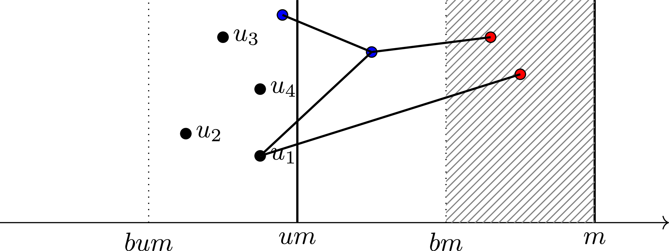
 u1,…,u4
 u1
u1 [bum,m]
 [bm,m]
 X1
X1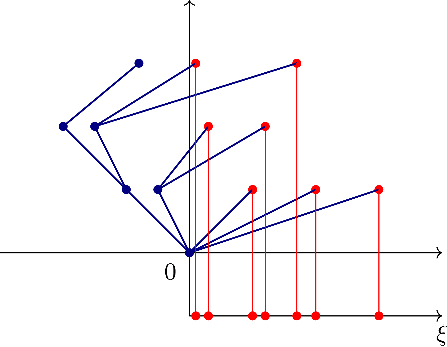
 [0,∞)
[0,∞) ξ
ξ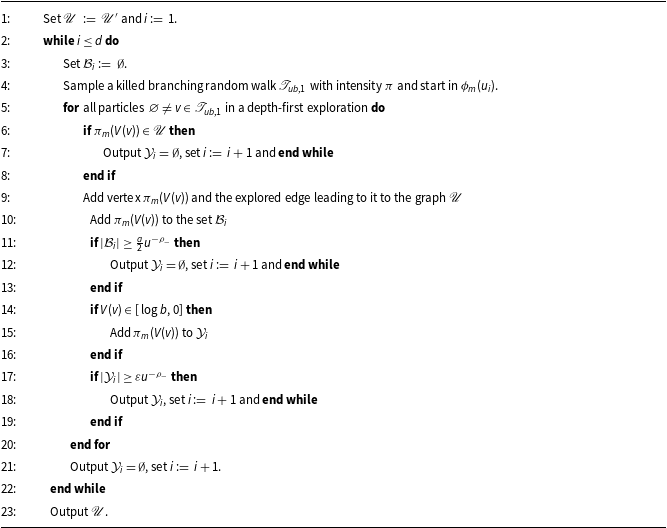

 Open access