1. Introduction
With the continuous increase in vehicle ownership, parking lots are in short supply, leading to the parking lots and the space near the parking spots (SNPS) becoming increasingly narrow, thus rendering manual parking operations more challenging [Reference Cai, Guan, Zhou, Xu, Jia and Zhan1]. Unskilled parking operations may disturb the surrounding road users and potentially cause traffic jams [Reference Chen, Gao, Hu, Du and Wang2]. Besides that, inexperienced drivers who are reluctant to try narrow parking lots would have to drive for longer periods of time and distance, thereby contributing to additional air pollution, fuel consumption, and congestion [Reference Rajabioun and Ioannou3]. Therefore, automatic parking technology for narrow parking spaces has gradually become a research focus [Reference Kim, Ahn and Park4].
The existing literature review centers on four techniques for automatic parking path planning. In specific parking situations, geometric approaches are applied [Reference Cai, Guan, Zhang, Jia and Zhan5], leveraging analytical expressions to rapidly pinpoint key trajectory points. For instance, Han [Reference Han6] put forward a geometric collision-free path planning method. Additionally, Clothoid, Bezier, and spline curves are utilized for path smoothing [Reference Vorobieva, Glaser, Minoiu-Enache and Mammar7]. Search methods discretize the continuous space into grids and search for a feasible parking path. Dolgov et al. [Reference Dolgov, Thrun, Montemerlo and Diebel8] introduced the Hybrid A* algorithm with Reeds-Shepp curve, which takes vehicle kinematics into account and employs more suitable heuristic functions. Subsequently, enhancement strategies are devised to boost path security, adaptability, and planning efficiency [Reference Lian, Ren, Yang, Li and Yu9, Reference Meng, Yang, Huang, Jin, Zhang, Jia, Wan, Xiao, Yang and Zhong10]. Sampling methods generate sample points in continuous space and aim to find a kinematically feasible and obstacle-avoiding point sequence as the planning outcome. Kuwata et al. [Reference Kuwata, Teo, Fiore, Karaman, Frazzoli and How11] considered vehicle kinematic constraints, assessed sampling-point feasibility via Dubins path length, and expanded nodes accordingly. To improve computational efficiency, Han et al. [Reference Han, Do and Mita12] proposed the Bidirectional Rapidly Random Tree (RRT) algorithm. Numerical optimization methods formulate trajectory planning as optimal control problems [Reference Bergman, Ljungqvist and Axehill13]. Proper description and handling of obstacle-avoidance constraints are vital for parking trajectory planning using these methods [Reference Li, Acarman, Zhang, Ouyang, Yaman, Kong, Zhong and Peng14]. Algorithms like Particle Swarm Optimization and Genetic Algorithm are employed to solve path optimization problems. Wang et al. [Reference Wang, Li, Yang, Meng and Fu15] proposed a hierarchical algorithm combining nonlinear optimization and an improved RRT with Reeds-Shepp curves to address inefficiencies and discontinuous curvature in parking trajectory planning, enabling continuous-curvature paths across diverse scenarios. Yang et al. [Reference Yang, Wang, Li, Meng, Jiang and Lu16] proposed a Sobol-RRT algorithm with Reeds-Shepp curves and optimal control to improve parking efficiency and dynamic obstacle handling in four-wheel steering vehicles. Li et al. [Reference Li, Li, Wu, Deng, Wang, Meng, Li, Su, Wang and Wang17] presented a Kinodynamic-Informed-Bidirectional Rapidly-exploring Random Tree Star algorithm to reduce unnecessary exploration near concave obstacles and generate kinematically admissible paths.
Based on the above-mentioned path planning methods, a general automatic parking system (APS) was developed in conjunction with the vehicle control system [Reference Khan and Guivant18]. In recent years, with the rapid advancement of artificial intelligence, end-to-end APS [Reference Mero, Yi, Dianati and Mouzakitis19], which integrates the path planning module and path tracking control module, has emerged. It directly outputs control variables to control the vehicle based on environmental information. Current implementation methods for end-to-end APS are deep learning and deep reinforcement learning (DRL) [Reference Teng, Chen, Ai, Zhou, Xuanyuan and Hu20]. It offers significant advantages not only in the end-to-end parking system but also in the parking lot allocation system [Reference Zhang, Zhao, Liao, Li and Du21]. Many researchers have conducted numerous studies on this. Zhang et al. [Reference Zhang, Xiong, Yu, Fang, Yan, Yao and Zhou22] proposed a DRL-based APS and compared its parking performance with that of a general APS. The results indicated that the DRL-based APS could park more easily with fewer deviations. Chai et al. [Reference Chai, Niu, Carrasco, Arvin, Yin and Lennox23] proposed an improved DNN-based motion planning algorithm and a DRL-based online collision avoidance approach in uncertain environments. Song et al. [Reference Song, Chen, Sun and Liu24] developed a parking model using actual parking data, addressing the limitation of model-free RL that requires extensive interactive data and enhancing training efficiency. Bernhard et al. [Reference Bernhard, Gieselmann, Esterle and Knol25] applied experience-based heuristic DRL to automatic parking, using human expertise to evaluate the explored data. Zhang et al. [Reference Zhang, Chen, Song and Hu26] regarded parking as a multi-objective optimization process considering safety, comfort, parking efficiency, and the FPS. Chai et al. [Reference Chai, Liu, Liu, Tsourdos, Xia and Chai27] designed a multilayer control scheme combining optimal trajectory planning and deep learning to guide the parking maneuver of autonomous ground vehicles (AGVs), and in [Reference Chai, Tsourdos, Savvaris, Chai, Xia and Chen28], they developed a novel RDNN-based motion planning approach for real-time parking movement planning of different AGVs. The end-to-end APS can solve path planning problems in uncertain dynamic environments. Nevertheless, it has the following drawbacks: limited generalization ability, a sharp decline in performance as the training task difficulty increases, and overly long training times for the system model [Reference Tang, Yang, Liu, Lin, Yang and Li29].
The above methods can enhance parking efficiency, reduce search time, and adapt to conventional parking spots. However, due to the constraints of narrow parking spaces and the limitations of drivers’ skills, the final parking state (FPS) of the vehicle often deviates, leading to partial encroachment into target parking spots and increased risk of collision during parking [Reference Chen, Gao, Hu, Du and Wang2, Reference Jin, Li, Lv and Zhang30]. For narrow spaces, Lian et al. [Reference Lian, Ren, Yang, Li and Yu31] designed an enhanced hybrid A* algorithm to address the search problem in narrow and complex environments. Li and Wang [Reference Li and Wang32] proposed a parallel parking path planning method in narrow spaces based on a three-stage curve interpolation approach. Vorobieva et al. [Reference Vorobieva, Glaser, Minoiu-Enache and Mammar7] designed a parallel parking path within small parking spaces using a continuous curvature curve improved by a clothoid curve. Li and Shao [Reference Li, Acarman, Peng, Zhang, Bian and Kong33] put forward a unified motion planning method for autonomous vehicle parking, which can effectively achieve path planning in the presence of irregularly placed obstacles. However, due to the comprehensive consideration of various factors, its real-time performance is slightly weak. Regarding non-standard scenarios, Tang et al. [Reference Tang, Yang, Liu, Lin, Yang and Li29] proposed a segmented parking training framework based on soft actor-critic to reduce the impact of vehicle intrusion on safety. Nevertheless, this method is not suitable for unfamiliar scenarios because of the inherent characteristics of reinforcement learning.
Current methods are rarely applied to narrow non-ideal scenarios for vertical parking, and their performance remains uncertain. Furthermore, there is a lack of characterization for non-ideal parking scenarios resulting from intrusion and a corresponding evaluation index for these scenarios.
In light of these issues, the contributions of this study are summarized as follows: (1) Definition and Characterization of Non-Ideal Parking Scenarios: The study defines and characterizes non-ideal parking scenarios using the deviation angle and offset distance relative to the actual parking spot boundaries. (2) Safety Index and Fast Calculation for Non-ideal Parking scenarios: A safety index based on the minimum distance between vehicles and obstacles (DBVO) is introduced for non-ideal parking. A partition-based method for calculating the minimum DBVO is proposed to quickly update these scenarios, enabling adaptability to various intrusion scenarios. (3) Four-Phase Parking Path Pattern: A four-phase parking path pattern is developed for non-ideal scenarios, incorporating straight lines, arcs, and clothoids. This pattern provides greater flexibility for the entry path to enhance safety distance while ensuring curvature continuity. (4) Preferred method for Parking Manners: A preferred rapid method for parking manners, including parking direction and number of maneuvers, is proposed based on the spatial demands of each parking manner. (5) Two-Step Optimization Framework: A two-step optimization framework combining online and offline methods is established for path planning in non-ideal parking scenarios. The off-line computation of preliminary data improves the efficiency of the online calculations, facilitating effective real-time path planning. The first step focuses on optimizing the FPS and entry path for improved safety, while the second step aims to improve parking efficiency by optimizing the path beyond the parking spot, thus enhancing overall path quality.
2. Quantitative characterization of the safety of intrusion parking scenarios
2.1. Parking scenarios
This study investigates two types of parking scenarios: ideal and actual ones. The actual scenario takes into account the impact of the FPS deviation of adjacent vehicles. As shown in Figure 1, adjacent vehicles 1–4 are within the normal FPS, while vehicles 5-10 deviate from it. Thus, parking spots 1 and 2 represent ideal scenarios without intrusion, and parking spots 3 and 4 are actual scenarios with one-sided and two-sided intrusions, respectively.
Ideal parking scenarios and actual parking scenarios.

2.2. Safety index indicators for parking scenario with intrusion
The actual parking spot is determined by the edges of adjacent vehicles, as shown in Figure 2. For modeling purposes, a coordinate system $O_PXY$
is established with the geometric center of the original parking spot as the origin. The offset distance and angle of the left and right edges (
$O_PXY$
is established with the geometric center of the original parking spot as the origin. The offset distance and angle of the left and right edges ( $\Delta x_L$
,
$\Delta x_L$
, $\Delta x_R$
,
$\Delta x_R$
, $\Delta \beta _L$
and
$\Delta \beta _L$
and $\Delta \beta _R$
) are used to describe the parking scenario. Then, the coordinates of the four vertices of the actual parking spot are
$\Delta \beta _R$
) are used to describe the parking scenario. Then, the coordinates of the four vertices of the actual parking spot are
 \begin{align} \left \{ \begin{array}{l} x_{\text{LU}} = - \dfrac {W_{\text{P}}}{2} + \frac {L_{\text{P}}}{2} \cdot \cot \beta _{\text{L}} + \Delta x_{\text{L}}, \quad y_{\text{LU}} = \dfrac {L_{\text{P}}}{2}\\[8pt] x_{\text{LB}} = - \dfrac {W_{\text{P}}}{2} - \dfrac {L_{\text{P}}}{2} \cdot \cot \beta _{\text{L}} + \Delta x_{\text{L}}, \quad y_{\text{LB}} = -\dfrac {L_{\text{P}}}{2}\\[8pt] x_{\text{RU}} = \dfrac {W_{\text{P}}}{2} + \dfrac {L_{\text{P}}}{2} \cdot \cot \beta _{\text{R}} - \Delta x_{\text{R}}, \quad y_{\text{RU}} = \dfrac {L_{\text{P}}}{2}\\[8pt] x_{\text{RB}} = \dfrac {W_{\text{P}}}{2} - \dfrac {L_{\text{P}}}{2} \cdot \cot \beta _{\text{R}} - \Delta x_{\text{R}}, \quad y_{\text{RB}} = -\dfrac {L_{\text{P}}}{2} \end{array} \right . \end{align}
where $\Delta x_L$
and
$\Delta x_L$
and $\Delta x_R$
are the offset distances of the mid-points of the left and right edges, respectively.
$\Delta x_R$
are the offset distances of the mid-points of the left and right edges, respectively. $\beta _L$
and
$\beta _L$
and $\beta _R$
are the inclination angles of the left and right edges (
$\beta _R$
are the inclination angles of the left and right edges ( $\beta _L=\Delta \beta _L+\frac {\pi }{2}$
,
$\beta _L=\Delta \beta _L+\frac {\pi }{2}$
, $\beta _R=\Delta \beta _R+\frac {\pi }{2}$
), respectively.
$\beta _R=\Delta \beta _R+\frac {\pi }{2}$
), respectively. $L_P$
and
$L_P$
and $W_P$
are the length and width of the original parking lot, respectively.
$W_P$
are the length and width of the original parking lot, respectively.
The shape of the actual parking spot is only determined by the total offset distance $\Delta x_O$
(
$\Delta x_O$
( $\Delta x_O = \Delta x_L+\Delta x_R$
) and the offset angles
$\Delta x_O = \Delta x_L+\Delta x_R$
) and the offset angles $\Delta \beta _L$
and
$\Delta \beta _L$
and $\Delta \beta _R$
. Thus, the vectors
$\Delta \beta _R$
. Thus, the vectors $[\Delta x_O, \Delta \beta _L, \Delta \beta _R]$
are used to characterize the actual parking scenarios.
$[\Delta x_O, \Delta \beta _L, \Delta \beta _R]$
are used to characterize the actual parking scenarios.
Generally, SNPS, including the width of the corridor ( $W_C$
) and the front space (
$W_C$
) and the front space ( $S_F$
), is limited, resulting in a higher risk of collision during parking. The intrusion of adjacent vehicles further increases this risk. As shown in 2, to ensure safety, a rectangular expansion is applied to the vehicle boundary, the expansion distance indicated as
$S_F$
), is limited, resulting in a higher risk of collision during parking. The intrusion of adjacent vehicles further increases this risk. As shown in 2, to ensure safety, a rectangular expansion is applied to the vehicle boundary, the expansion distance indicated as $d_E$
, which is set at 0.1 m in this study. During the parking process, the ego vehicle is subject to constraints from the left, right, and upper sides, as well as bottom constraints defined by the boundaries of the actual parking spot. The minimum DBVO is used for safety evaluation.
$d_E$
, which is set at 0.1 m in this study. During the parking process, the ego vehicle is subject to constraints from the left, right, and upper sides, as well as bottom constraints defined by the boundaries of the actual parking spot. The minimum DBVO is used for safety evaluation.
Actual parking scenario model and safety characterization.

The vehicle state is generally characterized by the coordinates of the rear axle center point and heading angle, represented as $\boldsymbol{S} = [x_E, y_E, \theta ]$
. To take advantage of the vehicle’s symmetry, the state
$\boldsymbol{S} = [x_E, y_E, \theta ]$
. To take advantage of the vehicle’s symmetry, the state $\boldsymbol{S}_{OV}$
(
$\boldsymbol{S}_{OV}$
( $\boldsymbol{S}_{OV} = [x_{OV}, y_{OV}, \theta ]$
), based on the geometric center of the vehicle, is adopted for safety analysis. The conversion formula between these two states is
$\boldsymbol{S}_{OV} = [x_{OV}, y_{OV}, \theta ]$
), based on the geometric center of the vehicle, is adopted for safety analysis. The conversion formula between these two states is
 \begin{align} \left \{ \begin{array}{l} x_{\text{OV}} = x_{\text{E}} + \left ( \dfrac {L_{\text{V}}}{2} - l_{\text{R}} \right ) \cos \theta \\[8pt] y_{\text{OV}} = y_{\text{E}} + \left ( \dfrac {L_{\text{V}}}{2} - l_{\text{R}} \right ) \sin \theta \end{array} \right . \end{align}
where $(x_{OV}, y_{OV})$
are the coordinates of the geometric center of the vehicle.
$(x_{OV}, y_{OV})$
are the coordinates of the geometric center of the vehicle. $L_V$
is vehicle length.
$L_V$
is vehicle length. $l_R$
is length of vehicle rear overhang.
$l_R$
is length of vehicle rear overhang.
The process for calculating the minimum distance between the vehicle and each obstacle is as follows. For the left, right, and upper constraints, the coordinates of the four expanded vertices of the vehicle are first computed for each heading angle, assuming the vehicle’s center is at the origin.
 \begin{equation} \left [ \begin{array}{c} \mathbf{x}_{\text{V}}(\theta ) \\ \mathbf{y}_{\text{V}}(\theta ) \end{array} \right ] = \left [ \begin{array}{cc} \cos \theta & -\sin \theta \\ \sin \theta & \cos \theta \end{array} \right ] \left [ \begin{array}{c} \mathbf{x}_{\text{V}}(0) \\ \mathbf{y}_{\text{V}}(0) \end{array} \right ] \end{equation}
where $\boldsymbol{x}_V(\theta )$
and
$\boldsymbol{x}_V(\theta )$
and $\boldsymbol{y}_V(\theta )$
are the abscissa and ordinate vectors of the vehicle’s expanded vertexes (points A, B, C, D in Figure 2) for a heading angle of
$\boldsymbol{y}_V(\theta )$
are the abscissa and ordinate vectors of the vehicle’s expanded vertexes (points A, B, C, D in Figure 2) for a heading angle of $\theta$
.
$\theta$
.
Then, the minimum distances between the vehicle and the upper, left, and right obstacles in state of $S_{OV}$
are calculated as follows.
$S_{OV}$
are calculated as follows.
 \begin{align} \left \{ \begin{array}{l} d_{\mathrm{U}} = W_{\mathrm{C}}+\dfrac {L_{\mathrm{P}}}{2}-\left [\max \left (\mathbf{y}_{\mathrm{V}}(\theta )\right )+y_{\mathrm{OV}}\right ]\\[3pt] d_{\mathrm{R}}=\dfrac {W_{\mathrm{P}}}{2}+S_{\mathrm{F}}-\left [\max \left (\mathbf{x}_{\mathrm{V}}(\theta )\right )+x_{\mathrm{OV}}\right ]\\[3pt] d_{\mathrm{L}}=\min \left (\mathbf{x}_{\mathrm{V}}(\theta )\right )+x_{\mathrm{OV}}-\dfrac {W_{\mathrm{P}}}{2}-S_{\mathrm{F}} \end{array} \right . \end{align}
where $d_U$
,
$d_U$
, $d_R$
, and
$d_R$
, and $d_L$
are the minimum distances between the vehicle and the upper, left, and right obstacles, respectively, with negative values indicating a collision.
$d_L$
are the minimum distances between the vehicle and the upper, left, and right obstacles, respectively, with negative values indicating a collision.
As illustrated in Figure 2, the bottom constraint consists of five line segments. Collision detection should be performed first, which involves checking for any interference between the four line segments of the vehicle’s expanded profile and the five line segments of the obstacles in the bottom constraint. The specific method is as follows.
 \begin{align} {f_{{\mathrm{IN}}ij}} = \left \{ \begin{array}{cc} 0&{{\mathrm{no\, intersection\, point}}}\\[3pt]1&{{\mathrm{else}}} \end{array} \right .,i = 1,2, \cdots ,4;\,\,j = 1,2, \cdots ,5 \end{align}
where $f_{IN_{ij}}$
is a logical variable indicating whether there is an intersection point between line segment
$f_{IN_{ij}}$
is a logical variable indicating whether there is an intersection point between line segment $i$
of the vehicle’s expansion profile and the obstacle line segment
$i$
of the vehicle’s expansion profile and the obstacle line segment $j$
. A sum of
$j$
. A sum of $\sum f_{IN}=0$
indicates no collision with the bottom constraint; otherwise, a collision occurs.
$\sum f_{IN}=0$
indicates no collision with the bottom constraint; otherwise, a collision occurs.
When there is no collision, the minimum distance between the vehicle and the bottom constraint is determined by the smallest distance from the four expanded vertices of the ego vehicle to the five obstacle line segments, as well as the distances from the two convex points, $L_U$
and
$L_U$
and $R_U$
, of the actual parking lot to the four expanded edges of the vehicle. The distance from point
$R_U$
, of the actual parking lot to the four expanded edges of the vehicle. The distance from point $L_U$
to line segment
$L_U$
to line segment $AB$
is calculated as follows.
$AB$
is calculated as follows.
 \begin{align} d_{\mathrm{PL}i} = \left \{ \begin{array}{cc} \left | \mathrm{L}_{\mathrm{U}}\mathrm{L}_{\mathrm{U}_\bot } \right | & \angle \mathrm{L}_{\mathrm{U}}\mathrm{AB} \lt \dfrac {\pi }{2} \cap \angle \mathrm{L}_{\mathrm{U}}\mathrm{BA} \lt \frac {\pi }{2}\\[3pt] \min \left ( \left | \mathrm{L}_{\mathrm{U}}\mathrm{A} \right |, \left | \mathrm{L}_{\mathrm{U}}\mathrm{B} \right | \right ) & \text{else} \end{array} \right .,\quad i = 1, \cdots , 28 \end{align}
Thus, the minimum distance between the vehicle and the bottom constraint ( $d_B$
) is
$d_B$
) is
 \begin{align} {d_{\mathrm{B}}} = \left \{ \begin{array}{cc} {\min \left \{ {{{\bf{d}}_{{\mathrm{PL}}}}} \right \}}&{\sum {{f_{{\mathrm{IN}}}}} = 0}\\[3pt] { - 0.1}&{\sum {{f_{{\mathrm{IN}}}}} \ne 0} \end{array} \right . \end{align}
2.3. Partition-based calculation method for $d_{B}$
field
$d_{B}$
field

Calculating the minimum $\text{DBVO}$
for safety evaluation during the path planning phase can significantly reduce planning efficiency, as the calculation of
$\text{DBVO}$
for safety evaluation during the path planning phase can significantly reduce planning efficiency, as the calculation of $d_B$
involves numerous interference detection and distance computations from points to line segments for each node in every path during the search process. To achieve real-time parking path planning, a method based on partition for calculating the
$d_B$
involves numerous interference detection and distance computations from points to line segments for each node in every path during the search process. To achieve real-time parking path planning, a method based on partition for calculating the $d_B$
field is proposed.
$d_B$
field is proposed.
As shown in Figure 3, under a constant heading angle, the trace of the vehicle’s geometric center – formed as the vehicle bottom slides along the bottom constraint line – divides the SNPS into three zones: the collision zone, the regular zone, and the key zone. The $d_B$
along the trace is zero. In the regular zone, the increment in
$d_B$
along the trace is zero. In the regular zone, the increment in $d_B$
equals the increment in the ordinate, as follows:
$d_B$
equals the increment in the ordinate, as follows:
 \begin{equation} {d_{\mathrm{B}}}(x,y,\theta ) = {d_{\mathrm{B}}}(x,{y_{{\mathrm{OV1}}}},\theta ) + y - {y_{{\mathrm{OV1}}}} \end{equation}
where (x, y) are the coordinates of the geometric center of the vehicle. $y_{OV1}$
is the vertical coordinate of the vehicle geometric center when its lower-right vertex of the expansion boundary is at the top-left vertex position of the parking space.
$y_{OV1}$
is the vertical coordinate of the vehicle geometric center when its lower-right vertex of the expansion boundary is at the top-left vertex position of the parking space.
Due to the symmetry of the vehicle,
 \begin{equation} {d_{\mathrm{B}}}(x,y,\theta ) = {d_{\mathrm{B}}}(x,y,\pi + \theta ) \end{equation}
Therefore, only the $d_B$
in the key zones within the heading angle range of
$d_B$
in the key zones within the heading angle range of $[0, \pi ]$
needs to be calculated to obtain the
$[0, \pi ]$
needs to be calculated to obtain the $d_B$
field of the entire
$d_B$
field of the entire $\text{SNPS}$
. As illustrated in Figure 3, the area of the key zones is substantially smaller than that of the entire
$\text{SNPS}$
. As illustrated in Figure 3, the area of the key zones is substantially smaller than that of the entire $\text{SNPS}$
, which leads to a marked improvement in computational efficiency.
$\text{SNPS}$
, which leads to a marked improvement in computational efficiency.
Partition of SNPS.

According to the relationship between the heading angle $\theta$
and the three angles of
$\theta$
and the three angles of $\pi /2$
,
$\pi /2$
, $\beta _L$
, and
$\beta _L$
, and $\beta _R$
, there are eight distinct partition situations. As illustrated in Figure 3, which represents the case where
$\beta _R$
, there are eight distinct partition situations. As illustrated in Figure 3, which represents the case where $\theta \lt \pi /2$
,
$\theta \lt \pi /2$
, $\theta \lt \beta _L$
, and
$\theta \lt \beta _L$
, and $\theta \lt \beta _R$
, the coordinates of the six critical points (
$\theta \lt \beta _R$
, the coordinates of the six critical points ( $x_{OVi}$
,
$x_{OVi}$
, $y_{OVi}$
) essential for the partitioning process are derived through geometric analysis.
$y_{OVi}$
) essential for the partitioning process are derived through geometric analysis.
 \begin{align} \left \{ \begin{array}{l} x_{\mathrm{OV}1} = x_{\mathrm{LU}} + L\cos (\gamma + \theta ),\quad y_{\mathrm{OV}1} = \dfrac {L_{\mathrm{P}}}{2} + L\sin (\gamma + \theta )\\[6pt] x_{\mathrm{OV}2} = x_{\mathrm{LU}} + L\cos (\gamma - \theta ),\quad y_{\mathrm{OV}2} = \dfrac {L_{\mathrm{P}}}{2} - L\sin (\gamma - \theta )\\[3pt] x_{\mathrm{OV}3} = (y_{\mathrm{OV}3} - y_{\mathrm{OV}2})\cot \beta _{\mathrm{L}} + x_{\mathrm{OV}2},\quad y_{\mathrm{OV}3} = -\dfrac {L_{\mathrm{P}}}{2} + L\sin (\gamma + \theta )\\[3pt] x_{\mathrm{OV}4} = x_{\mathrm{RB}} - L_{\mathrm{VE}}\cos \theta - L_{\mathrm{VE}}\sin \theta \cot \beta _{\mathrm{R}} + L\cos (\gamma + \theta ),\quad y_{\mathrm{OV}4} = y_{\mathrm{OV}3}\\[3pt] x_{\mathrm{OV}5} = (y_{\mathrm{OV}5} - y_{\mathrm{OV}4})\cot \beta _{\mathrm{R}} + x_{\mathrm{OV}4},\quad y_{\mathrm{OV}5} = \dfrac {L_{\mathrm{P}}}{2} + L\sin (\gamma - \theta )\\[3pt] x_{\mathrm{OV}6} = (y_{\mathrm{OV}5} - y_{\mathrm{OV}5})\cot \theta + x_{\mathrm{OV}5},\quad y_{\mathrm{OV}6} = \dfrac {L_{\mathrm{P}}}{2} + L\sin (\gamma + \theta ) \end{array} \right . \end{align}
where $\gamma$
is the angle between the diagonal of the expanding vehicle and the vehicle’s side.
$\gamma$
is the angle between the diagonal of the expanding vehicle and the vehicle’s side. ${L}=|\mathrm{AC}|/2$
.
${L}=|\mathrm{AC}|/2$
.
If the trace formed while sliding along the left side ( $OV_1 - OV_2 - OV_3$
) is positioned to the right of the trace formed while sliding along the right side (
$OV_1 - OV_2 - OV_3$
) is positioned to the right of the trace formed while sliding along the right side ( $OV_4 - OV_5 - OV_6$
), the enclosed area constitutes the collision zone, as illustrated by the shaded region in Figure 3. The remaining enclosed area is designated as the key zone. Similarly, key zones for the other seven situations can be determined.
$OV_4 - OV_5 - OV_6$
), the enclosed area constitutes the collision zone, as illustrated by the shaded region in Figure 3. The remaining enclosed area is designated as the key zone. Similarly, key zones for the other seven situations can be determined.
In conclusion, the total minimum $\text{DBVO}$
is given by:
$\text{DBVO}$
is given by:
 \begin{equation} {d_{\mathrm{A}}} = \min \left ( {{d_{\mathrm{U}}},{d_{\mathrm{B}}},{d_{\mathrm{L}}}\text{ or }{d_{\mathrm{R}}}} \right ) \end{equation}
The calculations for $d_U$
,
$d_U$
, $d_L$
, and
$d_L$
, and $d_R$
are relatively straightforward. Thus, computing the
$d_R$
are relatively straightforward. Thus, computing the $d_B$
field prior to path optimization and utilizing it during path search for safety detection can significantly enhance the computational efficiency of path planning.
$d_B$
field prior to path optimization and utilizing it during path search for safety detection can significantly enhance the computational efficiency of path planning.
3. Parking path design for intrusion scenarios based on predefined geometric set
3.1. Design of parking path curve
In traditional path planning, abrupt changes in curvature occur between straight lines and arcs (transitioning from $0$
to
$0$
to $\frac {1}{R}$
), which complicates the parking process. To address this issue, some researchers have employed clothoids to ensure curvature continuity in the optimal paths derived from combinations of straight lines and arcs, thereby enhancing the quality of parking paths. However, this approach increases the spatial requirements for parking, which poses significant safety challenges in narrow spaces [Reference Wu, Li, Gao and Yang34]. To overcome these challenges, a Clothoid-Aca-Clothoid (CAC) curve, characterized by curvature values of
$\frac {1}{R}$
), which complicates the parking process. To address this issue, some researchers have employed clothoids to ensure curvature continuity in the optimal paths derived from combinations of straight lines and arcs, thereby enhancing the quality of parking paths. However, this approach increases the spatial requirements for parking, which poses significant safety challenges in narrow spaces [Reference Wu, Li, Gao and Yang34]. To overcome these challenges, a Clothoid-Aca-Clothoid (CAC) curve, characterized by curvature values of $0$
at both the beginning and end, is proposed as an alternative to circular arcs. This CAC curve is directly applied in path optimization to ensure safer parking in tiny spaces.
$0$
at both the beginning and end, is proposed as an alternative to circular arcs. This CAC curve is directly applied in path optimization to ensure safer parking in tiny spaces.
Figure 4 presents a schematic illustration of the CAC curve, where $\delta _{Cm}$
is the maximum central angle of the clothoid, and
$\delta _{Cm}$
is the maximum central angle of the clothoid, and $\delta _{T}$
is the central angle of the CAC curve. As depicted in Figure 4 (a), when the center angle of CAC
$\delta _{T}$
is the central angle of the CAC curve. As depicted in Figure 4 (a), when the center angle of CAC $\delta _{T}\gt 2\delta _{Cm}$
, the CAC curve comprises two clothoids and an arc segment. Referring to Figure 4(c), it is evident that the curvature of this curve remains continuous, peaking at
$\delta _{T}\gt 2\delta _{Cm}$
, the CAC curve comprises two clothoids and an arc segment. Referring to Figure 4(c), it is evident that the curvature of this curve remains continuous, peaking at $\frac {1}{R_{min}}$
. However, when
$\frac {1}{R_{min}}$
. However, when $\delta _{T}\leq 2\delta _{Cm}$
, as illustrated in Figure 4 (b), the CAC curve simplifies to just two clothoids. In this case, the maximum curvature of the curve stands at
$\delta _{T}\leq 2\delta _{Cm}$
, as illustrated in Figure 4 (b), the CAC curve simplifies to just two clothoids. In this case, the maximum curvature of the curve stands at $\sqrt {\delta _{T}{\sigma }}$
. The detailed design of CAC curve can be found in the appendix.
$\sqrt {\delta _{T}{\sigma }}$
. The detailed design of CAC curve can be found in the appendix.
As demonstrated in Figure 4 (d), the CAC curve, upon undergoing mirroring, translation, and rotation, transforms into the essential components of the parking path. Here, there exist four distinct CAC paths that originate from the initial state $S_{0}=[x_{0}, y_{0}, \theta _{0}]$
and share a center angle
$S_{0}=[x_{0}, y_{0}, \theta _{0}]$
and share a center angle $\delta _{T}$
. These paths can be unambiguously determined based on the rotation angle (
$\delta _{T}$
. These paths can be unambiguously determined based on the rotation angle ( $\delta _R=\theta _{0}$
or
$\delta _R=\theta _{0}$
or $\theta _{0}+\pi$
) and the mirror logic variable (
$\theta _{0}+\pi$
) and the mirror logic variable ( $f_{M}=1$
or
$f_{M}=1$
or $- 1$
), which are determined according to the path function. The parameters of CAC path (
$- 1$
), which are determined according to the path function. The parameters of CAC path ( $x_{c}, y_{c}$
and
$x_{c}, y_{c}$
and $\theta _{c}$
) can be derived as follows.
$\theta _{c}$
) can be derived as follows.
 \begin{align} \begin{cases} x_{\mathrm{c}} = x_{\mathrm{c0}} \cdot \cos \delta _{\mathrm{R}} - f_{\mathrm{M}} \cdot y_{\mathrm{c0}} \cdot \sin \delta _{\mathrm{R}} + x_0 \\[3pt] y_{\mathrm{c}} = x_{\mathrm{c0}} \cdot \sin \delta _{\mathrm{R}} + f_{\mathrm{M}} \cdot y_{\mathrm{c0}} \cdot \cos \delta _{\mathrm{R}} + y_0 \\[3pt] \theta _{\mathrm{c}} = f_{\mathrm{M}} \cdot \theta _{\mathrm{c0}} + \theta _0 \end{cases} \end{align}
where $x_{c0}, y_{c0}$
and
$x_{c0}, y_{c0}$
and $\theta _{c0}$
are the coordinates and heading angle of the original CAC curve, respectively.
$\theta _{c0}$
are the coordinates and heading angle of the original CAC curve, respectively. $f_{M}$
is a logical variable signifying whether a path needs to be mirrored, with a value of
$f_{M}$
is a logical variable signifying whether a path needs to be mirrored, with a value of $-1$
indicating mirroring.
$-1$
indicating mirroring.
For simplicity in our discussion, the CAC curve obtained through the processes of mirroring, rotation, and translation is denoted as:
 \begin{equation} \mathrm{path\_CAC} \, = \, f_{\text{CAC}}(\mathbf{S}_0, \delta _{\mathrm{T}}, f_{\mathrm{M}}, \delta _{\mathrm{R}}) \end{equation}
CAC for parking path.

3.2. Design of parking path in intrusion scenarios
Due to the intrusion into the parking spot, the current vertical straight parking path presents a significant risk of collision. To address this, a four-phase parking path pattern is created, as illustrated in Figure 5. The entire parking path, extending from the starting state $S_{s}$
near the target parking spot to FPS
$S_{s}$
near the target parking spot to FPS $S_{e}$
, is segmented into four distinct phases: the transition path, maneuver path, entry path, and adjustment path. This path is composed of CAC curves and straight lines. The path can be determined using a reverse design approach, with the specific process detailed as follows.
$S_{e}$
, is segmented into four distinct phases: the transition path, maneuver path, entry path, and adjustment path. This path is composed of CAC curves and straight lines. The path can be determined using a reverse design approach, with the specific process detailed as follows.
Four-phase parking path pattern.

3.2.1. Adjustment path and entry path
The entry path is a sloping straight line, while the adjustment path is a CAC curve, as depicted in Figure 6. If the FPS of the vehicle is $S_{e}=[x_{e}, y_{e}, \theta _{e}]$
and the inclination angle of the entry path is
$S_{e}=[x_{e}, y_{e}, \theta _{e}]$
and the inclination angle of the entry path is $\theta _{L}$
, then the total center angle of the CAC curve for adjustment path is
$\theta _{L}$
, then the total center angle of the CAC curve for adjustment path is $\delta _{T} = |\theta _{L}-\theta _{e}|$
. Furthermore, if
$\delta _{T} = |\theta _{L}-\theta _{e}|$
. Furthermore, if $\theta _{L}-\theta _{e}\lt 0$
, the CAC curve must be mirrored for both forward and reverse parking scenarios.
$\theta _{L}-\theta _{e}\lt 0$
, the CAC curve must be mirrored for both forward and reverse parking scenarios.
For reverse parking, the original CAC curve needs to be rotated by $\theta _{e}$
. Consequently, the adjustment path is given by:
$\theta _{e}$
. Consequently, the adjustment path is given by:
 \begin{equation} \mathrm{path\_A} = f_{\text{CAC}}\left (\mathbf{S}_{\mathrm{e}}, \left | \theta _{\mathrm{L}} - \theta _{\mathrm{e}} \right |, \text{sign}(\theta _{\mathrm{L}} - \theta _{\mathrm{e}}), \theta _{\mathrm{e}}\right ) \end{equation}
For forward parking, the original CAC curve needs to be rotated by $\theta _{e}+\pi$
, thus:
$\theta _{e}+\pi$
, thus:
 \begin{equation} \mathrm{path\_A} = f_{\text{CAC}}\left (\mathbf{S}_{\mathrm{e}}, \left | \theta _{\mathrm{L}} - \theta _{\mathrm{e}} \right |, \text{sign}(\theta _{\mathrm{L}} - \theta _{\mathrm{e}}), \theta _{\mathrm{e}} + \pi \right ) \end{equation}
After determining the state adjustment path, the lower node state $S_{L}$
of the entry path (Path_E) can be calculated. Hence, with the FPS known, the entry path and state adjustment path can be defined by the ordinate
$S_{L}$
of the entry path (Path_E) can be calculated. Hence, with the FPS known, the entry path and state adjustment path can be defined by the ordinate $y_{M1}$
of the upper node of the entry path and
$y_{M1}$
of the upper node of the entry path and $\theta _{L}$
.
$\theta _{L}$
.
Four-phase parking path pattern.

3.2.2. Maneuver path
The maneuver path consists of CAC curves, with the number of curves determined by the required maneuvers, as shown in Figure 7. The vector representing the center angles of these CAC curves is denoted as $\boldsymbol{\delta }=[\delta _{1},\delta _{2},\cdots ,\delta _{n}]$
. As illustrated in Figure 7 (a) and (c), when the vehicle approaches from the left, the heading angle changes from
$\boldsymbol{\delta }=[\delta _{1},\delta _{2},\cdots ,\delta _{n}]$
. As illustrated in Figure 7 (a) and (c), when the vehicle approaches from the left, the heading angle changes from $0$
to
$0$
to $\theta _{L}$
. Conversely, when approaching from the right, the heading angle changes from
$\theta _{L}$
. Conversely, when approaching from the right, the heading angle changes from $\pi$
to
$\pi$
to $\theta _{L}$
, as shown in Figure 7 (b) and (d). Thus, the sum of the total center angles of all CAC curves in the maneuver path is
$\theta _{L}$
, as shown in Figure 7 (b) and (d). Thus, the sum of the total center angles of all CAC curves in the maneuver path is
 \begin{align} \delta _{\mathrm{A}} = \sum _{i = 1}^{n} \delta _{i} = \begin{cases} \left | \theta _{\mathrm{L}} \right | & f_{\mathrm{L}} = 1 \\[3pt] \pi - \left | \theta _{\mathrm{L}} \right | & f_{\mathrm{L}} = -1 \end{cases} \end{align}
where $f_L$
is a logical variable indicating whether the vehicle approaches from the left. In state
$f_L$
is a logical variable indicating whether the vehicle approaches from the left. In state $S_{M1}$
, the heading angle
$S_{M1}$
, the heading angle $\theta _{M1}=\theta _L$
. The heading angles of other node states
$\theta _{M1}=\theta _L$
. The heading angles of other node states $S_{M2}\sim S_{Mn}$
are given by:
$S_{M2}\sim S_{Mn}$
are given by:
 \begin{equation} \begin{cases} \theta _{\mathrm{M}i} = \theta _{\mathrm{L}} - \sum _{j = 1}^{i - 1} \delta _{j}, \quad i = 2, \cdots , n \end{cases} \end{equation}
where $n$
is number of maneuvers.
$n$
is number of maneuvers.
As shown in Figure 7(a) and (b), in the situations of reverse parking, the first maneuver path ( $S_{M1}\sim S_{M2}$
) when vehicles approach from the left is obtained by rotating the mirrored original CAC by
$S_{M1}\sim S_{M2}$
) when vehicles approach from the left is obtained by rotating the mirrored original CAC by $\theta _{M1}$
and then translating it to
$\theta _{M1}$
and then translating it to $(x_{M1}, y_{M1})$
. The second maneuver path (
$(x_{M1}, y_{M1})$
. The second maneuver path ( $S_{A2}\sim S_{A3}$
) is obtained by rotating the mirrored original CAC by
$S_{A2}\sim S_{A3}$
) is obtained by rotating the mirrored original CAC by $\theta _{A2}+\pi$
and then translating it to
$\theta _{A2}+\pi$
and then translating it to $(x_{M2}, y_{M2})$
. The third section follows the pattern of the first, and the fourth section is similar to the second one. When the vehicle approaches from the right, the rotation angle of the original CAC curve remains the same as when approaching from the left, but the CVC curves do not require mirroring. In summary, the
$(x_{M2}, y_{M2})$
. The third section follows the pattern of the first, and the fourth section is similar to the second one. When the vehicle approaches from the right, the rotation angle of the original CAC curve remains the same as when approaching from the left, but the CVC curves do not require mirroring. In summary, the $i$
-th (
$i$
-th ( $i = 1,\ldots , n$
) section of the maneuver path for reverse parking is
$i = 1,\ldots , n$
) section of the maneuver path for reverse parking is
 \begin{equation} \mathrm{path\_}M_{i} = f_{\text{CAC}}\left (\mathbf{S}_{M_{i}}, \delta _{i}, -f_{\mathrm{L}}, \theta _{M_{i}} + \left [ 1 + (\!-1)^{i} \right ] \cdot \frac {\pi }{2} \right ) \end{equation}
Similarly, the $i$
-th (
$i$
-th ( $i = 1,\ldots ,n$
) section of the maneuver path for forward parking can be derived.
$i = 1,\ldots ,n$
) section of the maneuver path for forward parking can be derived.
 \begin{equation} \mathrm{path\_}M_{i} = f_{\text{CAC}}\left (\mathbf{S}_{M_{i}}, \delta _{i}, f_{\mathrm{L}}, \theta _{M_{i}} + \left [ 1 + (\!-1)^{i + 1} \right ] \cdot \frac {\pi }{2} \right ) \end{equation}
Design of maneuver path.

Design of state path.

In the following, we present algorithms for offline planning with lead times in the order of tens of seconds to several minutes, depending on the complexity of the scenario and the desired quality of the solutions, and for online planning with computation times in the order of fractions of a second up to very few seconds. The algorithm for offline planning is based on a global optimization approach and ensures high-quality solutions. The algorithm for online planning uses a sequential optimization procedure that provides flight paths with slightly decreasing quality.
3.2.3. Transition path
As shown in Figure 8, the transition path consists of two CAC curves and a horizontal straight line segment. Its purpose is to move the vehicle from the starting state ( $S_S$
) to the starting state of the maneuver path (
$S_S$
) to the starting state of the maneuver path ( $S_{M_{n + 1}}$
). Based on the orientation of the vehicle in
$S_{M_{n + 1}}$
). Based on the orientation of the vehicle in $S_S$
and the vertical distance between
$S_S$
and the vertical distance between $S_S$
and
$S_S$
and $S_{M_{n+1}}$
, the transition path can be categorized into four scenarios.
$S_{M_{n+1}}$
, the transition path can be categorized into four scenarios.
To demonstrate the design process of the transition path, consider the first scenario depicted in Figure 8(a). If the vertical displacement of the CAC curve, initiated with a heading angle of $\theta _s$
and terminated at a heading angle of 0, precisely matches the value of
$\theta _s$
and terminated at a heading angle of 0, precisely matches the value of $y_{M_{n+1}}-y_s$
, the transition path can be efficiently constructed using a single CAC curve in conjunction with one linear segment. This optimal configuration is illustrated by the red curve in 8(a). In this case, the starting heading angle
$y_{M_{n+1}}-y_s$
, the transition path can be efficiently constructed using a single CAC curve in conjunction with one linear segment. This optimal configuration is illustrated by the red curve in 8(a). In this case, the starting heading angle $\theta _s$
is referred to as
$\theta _s$
is referred to as $\theta _{cr}$
:
$\theta _{cr}$
:
 \begin{equation} \theta _{\mathrm{cr}} = H_{\mathrm{C}0}^{-1}(y_{\mathrm{M}n + 1} - y_{\mathrm{s}}) \end{equation}
where $H_{C0}^{- 1}(y)$
is the inverse function of
$H_{C0}^{- 1}(y)$
is the inverse function of $H_C(\delta _T, \delta _R, f_M)$
with
$H_C(\delta _T, \delta _R, f_M)$
with $\delta _R = 0$
and
$\delta _R = 0$
and $f_M = 1$
.
$f_M = 1$
. $H_C(\delta _T, \delta _R, f_M)$
represents the vertical distance between the two endpoints of the original or mirrored CAC curve, with a center angle of
$H_C(\delta _T, \delta _R, f_M)$
represents the vertical distance between the two endpoints of the original or mirrored CAC curve, with a center angle of $\delta _T$
rotated by
$\delta _T$
rotated by $\delta _R$
.
$\delta _R$
. $H_{C0}(\delta _T)=H(\delta _T, 0, 1)$
. In this case, the CAC curve of the transition path is
$H_{C0}(\delta _T)=H(\delta _T, 0, 1)$
. In this case, the CAC curve of the transition path is
 \begin{equation} \mathrm{path\_}T_{\mathrm{C}} = f_{\text{CAC}}(\mathbf{S}_{\mathrm{s}}, \theta _{\mathrm{s}}, - 1, \theta _{\mathrm{s}}) \end{equation}
When $\theta _s\neq \theta _{cr}$
, the transition path requires two CAC curves (
$\theta _s\neq \theta _{cr}$
, the transition path requires two CAC curves ( $S_s\rightarrow S_{T1}$
and
$S_s\rightarrow S_{T1}$
and $S_{T1}\rightarrow S_{T2}$
). The key to determining these curves is to find the heading angle
$S_{T1}\rightarrow S_{T2}$
). The key to determining these curves is to find the heading angle $\theta _{T1}$
in
$\theta _{T1}$
in $S_{T1}$
. If
$S_{T1}$
. If $\theta _s\gt \theta _{cr}$
, the transition path will produce an overshoot as indicated by the blue dashed line in Figure 8(a), and
$\theta _s\gt \theta _{cr}$
, the transition path will produce an overshoot as indicated by the blue dashed line in Figure 8(a), and $\theta _{T1}$
must satisfy:
$\theta _{T1}$
must satisfy:
 \begin{equation} H_{\mathrm{C}}\left ( \left | \theta _{\mathrm{T}1} - \theta _{\mathrm{s}} \right |, \theta _{\mathrm{s}}, - 1 \right ) - H_{\mathrm{C}}\left ( - \theta _{\mathrm{T}1}, 0, 1 \right ) = y_{\mathrm{M}n + 1} - y_{\mathrm{s}} \end{equation}
If $\theta _s\gt \theta _{cr}$
, the transition path does not overshoot, and
$\theta _s\gt \theta _{cr}$
, the transition path does not overshoot, and $\theta _{T1}$
must satisfy the condition specified in Eq. (23). The corresponding transition path is represented by the solid green curve in Figure 8(a).
$\theta _{T1}$
must satisfy the condition specified in Eq. (23). The corresponding transition path is represented by the solid green curve in Figure 8(a).
 \begin{equation} H_{\mathrm{C}}\left ( \left | \theta _{\mathrm{T}1} - \theta _{\mathrm{s}} \right |, \theta _{\mathrm{s}}, 1 \right ) + H_{\mathrm{C}}\left ( \theta _{\mathrm{T}1}, 0, 1 \right ) = y_{\mathrm{M}n + 1} - y_{\mathrm{s}} \end{equation}
Using Eq. (22) or Eq. (23), $\theta _{T1}$
can be determined. Consequently, the two CAC curves for the transition path are
$\theta _{T1}$
can be determined. Consequently, the two CAC curves for the transition path are
 \begin{align} \left \{ \begin{array}{l} \mathrm{path\_}T_{\mathrm{C}1} = f_{\text{CAC}}\left ( \mathbf{S}_{\mathrm{s}}, \left | \theta _{\mathrm{T}1} - \theta _{\mathrm{s}} \right |, - 1, \theta _{\mathrm{s}} \right )\\[3pt] \mathrm{path\_}T_{\mathrm{C}2} = f_{\text{CAC}}\left ( \mathbf{S}_{\mathrm{T}1}, \theta _{\mathrm{T}1}, 1, \theta _{\mathrm{T}1} \right ) \end{array} \right . \end{align}
For the remaining three scenarios shown in Figure 8(b), (c), and (d), the CAC curves of the transition path can be derived through symmetry. These CAC curves and the horizontal line segment connecting $S_{T1}$
to
$S_{T1}$
to $S_{M_{n+1}}$
together form the complete transition path (path_T). In summary, given the starting and FPS of the vehicle, the parking path designed using the presented method can be determined by
$S_{M_{n+1}}$
together form the complete transition path (path_T). In summary, given the starting and FPS of the vehicle, the parking path designed using the presented method can be determined by $\delta$
,
$\delta$
, $\theta _L$
and
$\theta _L$
and $y_{M1}$
.
$y_{M1}$
.
4. Two-step optimization method of FPS and parking path
During the entry and state adjustment phases, the risk of collision is at its highest, making safety the primary concern. Conversely, in the transition and adjustment phases, efficiency takes precedence. Therefore, this paper proposes a two-step parking path optimization method that optimizes for safety and efficiency as objectives for different optimization steps.
4.1. Framework for two-step parking path optimization method
To enhance the computational efficiency of the two-step parking path optimization method, a framework that integrates both online and offline calculations has been developed, as illustrated in Figure 9. The offline calculations encompass the basic parameters of the CAC curve, the construction of the CAC curve set and its associated functions, the $d_B$
field in an ideal parking scenario, and the critical SNPS required for each parking manner.
$d_B$
field in an ideal parking scenario, and the critical SNPS required for each parking manner.
Framework of the two-step parking path optimization method.

The online calculation process begins after parking allocation. If the parking spot is invaded, the dB field is updated accordingly. Subsequently, the first step of optimization is performed. If a solution is found, the process advances to the second step. In the second step, the parking manner is determined based on the actual SNPS, followed by the optimization of the transition and maneuver paths. Ant colony algorithms [Reference Han, Zhou, Zhang, Wang, Liu, Peng and Guizani35] are employed to solve the optimization models.
4.2. Optimization of FPS and inclination angle of entry path
For safety, the minimum DBVO under bottom constraints ( $d_B$
) is taken as the index. The first-step optimization is to maximize
$d_B$
) is taken as the index. The first-step optimization is to maximize $d_B$
during the entry and adjustment phases. Accordingly, the objective function is defined as follows:
$d_B$
during the entry and adjustment phases. Accordingly, the objective function is defined as follows:
 \begin{equation} d_{\min 1} = \min \left [ d_{\mathrm{B}}(\mathrm{path\_E}, \mathrm{path\_A}) \right ] \end{equation}
The optimization parameters include the vehicle FPS and the inclination angle of the entry path. To simplify calculations, the state based on the vehicle’s geometric center is adopted. The parameter $y_{M1}$
is preset to determine the entry path for calculating the objective function.
$y_{M1}$
is preset to determine the entry path for calculating the objective function.
 \begin{equation} \mathbf{X}_1 = [x_{\mathrm{OVe}}, y_{\mathrm{OVe}}, \theta _{\mathrm{e}}, \theta _{\mathrm{L}}] \end{equation}
where $(x_{OVe}, y_{OVe})$
are coordinates of vehicle’s geometric center in FPS.
$(x_{OVe}, y_{OVe})$
are coordinates of vehicle’s geometric center in FPS.
The constraints are outlined as follows. The range for the geometric center of the vehicle in FPS is given by
 \begin{align} g_1^1(\mathbf{X}_1)\,: \left \{ \begin{array}{c} - 0.5 \leq x_{\mathrm{OVe}} \leq 0.5 \\[3pt] - 0.5 \leq y_{\mathrm{OVe}} \leq 0.5 \end{array} \right . \end{align}
This equation expands the allowable range for the geometric center, which may lead to the vehicle not being entirely within the parking spot; therefore, additional constraints are necessary:
 \begin{align} g_2^1(\mathbf{X}_1)\,: \left \{ \begin{array}{l} \max \left ( \mathbf{y}_{\mathrm{V}}(\theta _{\mathrm{e}}) + y_{\mathrm{OVe}} \right ) \leq \frac {L_P}{2} \\[3pt] d_{\min 1} \geq 0 \end{array} \right . \end{align}
The directions of the final heading angle and the inclination angle should be between the directions of the two side lines of the actual parking lot. When parking forward, the constraints are defined as
 \begin{align} g_3^1(\mathbf{X}_1)\,: \left \{ \begin{array}{l} -\max (\beta _{\mathrm{L}}, \beta _{\mathrm{R}}) \leq \theta _{\mathrm{e}} \leq -\min (\beta _{\mathrm{L}}, \beta _{\mathrm{R}}) \\[3pt] -\max (\beta _{\mathrm{L}}, \beta _{\mathrm{R}}) \leq \theta _{\mathrm{L}} \leq -\min (\beta _{\mathrm{L}}, \beta _{\mathrm{R}}) \end{array} \right . \end{align}
When parking in reverse, the conditions are
 \begin{align} g_3^1(\mathbf{X}_1)\,: \left \{ \begin{array}{l} \min (\beta _{\mathrm{L}}, \beta _{\mathrm{R}}) \leq \theta _{\mathrm{e}} \leq \max (\beta _{\mathrm{L}}, \beta _{\mathrm{R}}) \\[3pt] \min (\beta _{\mathrm{L}}, \beta _{\mathrm{R}}) \leq \theta _{\mathrm{L}} \leq \max (\beta _{\mathrm{L}}, \beta _{\mathrm{R}}) \end{array} \right . \end{align}
Thus, the optimization model for both FPS and entry path inclination angle is expressed as
 \begin{align} \begin{array}{cc} \max & d_{\min 1} \\[3pt] \text{s.t.} & \begin{array}{cc} g_i^1(\mathbf{X}_1) & i = 1,2,3 \end{array} \end{array} \end{align}
For the convenience of discussion, the optimal FPS based on the rear axle center is denoted as $S_{eO}$
, and the optimal inclination angle of the entry path is denoted as
$S_{eO}$
, and the optimal inclination angle of the entry path is denoted as $\theta _{LO}$
.
$\theta _{LO}$
.
4.3. Optimization of the maneuver and transition path
The maneuver and transition paths are defined by parameter $\delta$
and
$\delta$
and $y_{M1}$
. Therefore, the second step of optimization focuses on finding a set of maneuver path parameters that maximize parking efficiency. The parking efficiency is influenced by both the length of the parking path and the parking manner.
$y_{M1}$
. Therefore, the second step of optimization focuses on finding a set of maneuver path parameters that maximize parking efficiency. The parking efficiency is influenced by both the length of the parking path and the parking manner.
4.3.1. Optimization model of path length
The optimization function is based on the total length of the maneuver and transition path ( $l_{TM}$
), the calculation formula is
$l_{TM}$
), the calculation formula is
 \begin{equation} l_{\mathrm{TM}} = L_{\mathrm{C}}\left ( \left | \theta _{\mathrm{T}1} - \theta _{\mathrm{s}} \right | \right ) + L_{\mathrm{C}}\left ( \left | \theta _{\mathrm{T}1} \right | \right ) + \sum _{i = 1}^{n} L_{\mathrm{C}}\left ( \delta _{i} \right ) + \left | x_{\mathrm{T}2} - x_{\mathrm{M}n + 1} \right | \end{equation}
where $L_C(\delta )$
is the length of the CAC curve with a central angle of
$L_C(\delta )$
is the length of the CAC curve with a central angle of $\delta$
.
$\delta$
.
The optimization parameters include the ordinate of the starting point of the entry path and the center angle vector of the CAC curves of the maneuver path.
 \begin{equation} \mathbf{X}_2 = [y_{\mathrm{M}1}, \mathbf{\delta }] \end{equation}
The range of values for the ordinate $y_{M1}$
is defined as
$y_{M1}$
is defined as
 \begin{align} g_1^2(\mathbf{X}_2)\,: \left \{ \begin{array}{cc} y_{\mathrm{LO}} \leq y_{\mathrm{M1}} \leq W_{\mathrm{C}} + \frac {L_{\mathrm{P}}}{2} - l_{\mathrm{A}} - l_{\mathrm{F}} - d_{\mathrm{E}} & \text{Reverse} \\[3pt] y_{\mathrm{LO}} \leq y_{\mathrm{M1}} \leq W_{\mathrm{C}} + \frac {L_{\mathrm{P}}}{2} - l_{\mathrm{R}} - d_{\mathrm{E}} & \text{Forward} \end{array} \right . \end{align}
where $y_{LO}$
is the starting point ordinate of the adjustment path obtained from the first-step optimization.
$y_{LO}$
is the starting point ordinate of the adjustment path obtained from the first-step optimization. $l_F$
is length of vehicle front overhang.
$l_F$
is length of vehicle front overhang.
The constraint for the central angle vector $\delta$
is given by
$\delta$
is given by
 \begin{align} g_2^2(\mathbf{X}_2)\,: \left \{ \begin{array}{l} \sum _{i = 1}^{n} \delta _i = \delta _{\mathrm{A}} \\[3pt] \begin{array}{cc} 0 \lt \delta _i \leq \delta _{\mathrm{A}} & i = 1,2, \cdots , n \end{array} \end{array} \right . \end{align}
The vehicle’s FPS and the entry path inclination angle are set based on the results obtained from the first step of optimization.
 \begin{align} g_3^2(\mathbf{X}_2)\,: \left \{ \begin{array}{l} \mathbf{S}_{\mathrm{e}} = \mathbf{S}_{\mathrm{eO}} \\[3pt] \theta _{\mathrm{L}} = \theta _{\mathrm{LO}} \end{array} \right . \end{align}
To ensure non-collision, the minimum DBVO from the starting state to state $S_{M1}$
must be at least 0. Thus
$S_{M1}$
must be at least 0. Thus
 \begin{equation} g_4^2(\mathbf{X}_2)\,:\,d_{\min 2} = \min \left [ d_{\mathrm{A}}(\mathrm{path\_T},\mathrm{path\_M}) \right ] \geq 0 \end{equation}
Therefore, the optimization model for the path length is expressed as
 \begin{equation} \begin{array}{cc} \min & l_{\mathrm{TM}} \\ \text{s.t.} & \begin{array}{cc} g_i^2(\mathbf{X}_2) & i = 1,2,3,4 \end{array} \end{array} \end{equation}
4.3.2. Optimization of parking manners
Parking manners are influenced by the parking direction and the number of maneuvers required. As shown in Figure 10, forward parking with one maneuver (F1) does not involve any reversing, while forward parking with two or three maneuvers (F2 or F3) necessitates reversing the vehicle direction twice. In contrast, reverse parking with one or two maneuvers (R1 or R2) requires reversing only once, while reverse parking with three maneuvers (R3) requires reversing three times. Each reversal requires deceleration and acceleration, which not only decreases parking efficiency but also reduces passenger comfort. Additionally, compared to R1 and F2, R2 and F3 each involve one additional directional change operation, making vehicle control more challenging. Therefore, to minimize the number of reversals and directional changes, the priority order of parking manners, assuming no constraints on SNPS, is as follows: F1, R1, R2, F2, F3, and R3.
Maneuver path under different maneuvering times.

In actual parking scenarios, SNPS is limited, so parking manners must be optimized within SNPS constraints. Thus, it is necessary to analyze the SNPS requirements for various parking manners in intrusion scenarios. A multi-objective optimization model is established with the aim of minimizing both corridor width and front space, as represented by Eq. (39). By solving the Pareto optimal solution for this model, the critical SNPS required for each parking manner can be determined. Combining this with the priority order allows for the identification of the optimal parking manner.
 \begin{align} \begin{array}{cc} \min & f_{\mathrm{ob}}(\mathbf{X}_2) = \left [ W_{\mathrm{C}}, S_{\mathrm{F}} \right ] \\[3pt] \text{s.t.} & \left \{ \begin{array}{l} \begin{array}{cc} g_i^2(\mathbf{X}_2) & i = 1,2,3,4 \end{array} \\[3pt] \mathbf{S}_{\mathrm{e}} = \mathbf{S}_{\mathrm{eO}}, \theta _{\mathrm{L}} = \theta _{\mathrm{LO}} \\[3pt] \mathbf{S}_{\mathrm{s}} = [x_{\mathrm{s}}, y_{\mathrm{s}}, 0] \end{array} \right . \end{array} \end{align}
where
 \begin{align} \left \{ \begin{array}{l} W_{\mathrm{C}} = \max (\mathbf{y}_{\mathrm{V}}) - \dfrac {L_{\mathrm{P}}}{2}\\[8pt] S_{\mathrm{F}} = \left \{ \begin{array}{cc} \max (\mathbf{x}_{\mathrm{V}}) - \dfrac {W_{\mathrm{P}}}{2} & \text{From left}\\[3pt] - \dfrac {W_{\mathrm{P}}}{2} - \min (\mathbf{x}_{\mathrm{V}}) & \text{From right} \end{array} \right .\\[20pt] x_{\mathrm{s}} = \left \{ \begin{array}{cc} 10 & \text{From left}\\[5pt] -10 & \text{From right} \end{array} \right .\\[3pt] y_{\mathrm{s}} = 5 \end{array} \right . \end{align}
where $(x_s, y_s)$
is the starting position.
$(x_s, y_s)$
is the starting position.
5. Results and discussion
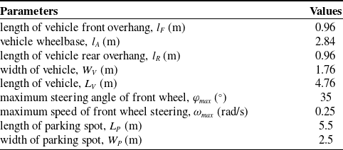
Using the dimensions of typical vehicles and parking spaces as a reference, the parameters are detailed in Table I.
 \begin{equation} \sigma = \frac {\omega }{v \cdot \varphi _{\max } \cdot R_{\min }} \end{equation}
According to Eq. (46), the minimum turning radius $R_{min}$
for the given vehicle is 4.06m. Additionally, a clothoid curve is generated when the vehicle’s speed remains constant while the steering angle of the front wheels changes uniformly. The rate of curvature change for the clothoid is given by Eq. (41), where
$R_{min}$
for the given vehicle is 4.06m. Additionally, a clothoid curve is generated when the vehicle’s speed remains constant while the steering angle of the front wheels changes uniformly. The rate of curvature change for the clothoid is given by Eq. (41), where $v$
is velocity of parking. Setting
$v$
is velocity of parking. Setting $\omega = \omega _{\max }$
, the value of
$\omega = \omega _{\max }$
, the value of $\sigma$
varies from 1 to 0.05 as
$\sigma$
varies from 1 to 0.05 as $v$
ranges from
$v$
ranges from $0.1\mathrm{m/s}$
to
$0.1\mathrm{m/s}$
to $2\mathrm{m/s}$
, based on the given vehicle parameters. Considering the required space and parking efficiency, a value of
$2\mathrm{m/s}$
, based on the given vehicle parameters. Considering the required space and parking efficiency, a value of $\sigma = 0.32$
is selected.
$\sigma = 0.32$
is selected.
Geometric structure parameters of vehicles and parking lot parameters.

5.1. Result of
$d_{B}$
field

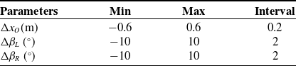
According to the statistical data from actual parking lots, the distribution range of parameters $[\Delta x_O, \Delta \beta _L, \Delta \beta _R]$
that characterize parking scenarios is shown in Table II. Through discretization for dB field calculation and analysis, 847 parking scenarios were generated. The simulation experiments were conducted on a computer with the following configuration: Intel (R) Core (TM) i9-10940X CPU @ 3.30 GHz, 16.0 GB RAM, and 12-thread parallel computing capabilities.
$[\Delta x_O, \Delta \beta _L, \Delta \beta _R]$
that characterize parking scenarios is shown in Table II. Through discretization for dB field calculation and analysis, 847 parking scenarios were generated. The simulation experiments were conducted on a computer with the following configuration: Intel (R) Core (TM) i9-10940X CPU @ 3.30 GHz, 16.0 GB RAM, and 12-thread parallel computing capabilities.
Figure 11 displays the calculation time for the $d_B$
field, with an ideal parking scenario taking
$d_B$
field, with an ideal parking scenario taking $8.73\mathrm{s}$
. Additionally, there are 84 parking scenarios without intrusion, for which the dB field of the ideal scenario can be used for path optimization. The remaining scenarios involve intrusions, and the average calculation time for their dB fields is
$8.73\mathrm{s}$
. Additionally, there are 84 parking scenarios without intrusion, for which the dB field of the ideal scenario can be used for path optimization. The remaining scenarios involve intrusions, and the average calculation time for their dB fields is $9.08\mathrm{s}$
, with the maximum time not exceeding
$9.08\mathrm{s}$
, with the maximum time not exceeding $25\mathrm{s}$
. Given that the time for a vehicle to travel from the parking space entrance to a nearby point in the target parking spot is longer than the dB field calculation time, the
$25\mathrm{s}$
. Given that the time for a vehicle to travel from the parking space entrance to a nearby point in the target parking spot is longer than the dB field calculation time, the $d_B$
field can be computed and updated online during this period.
$d_B$
field can be computed and updated online during this period.
The range and discrete interval of the intrusion scene representation parameters.

Calculation time for dB field.

Result of $d_{B}$
field. (a) Ideal parking scenarios; (b) Invaded parking scenarios.
$d_{B}$
field. (a) Ideal parking scenarios; (b) Invaded parking scenarios.

Figure 12 illustrates the dB field for both ideal and intrusive scenarios ( $[\Delta x_O, \Delta \beta _L, \Delta \beta _R]=[0\ 10\ 6]$
). In the entry and adjustment phases (when
$[\Delta x_O, \Delta \beta _L, \Delta \beta _R]=[0\ 10\ 6]$
). In the entry and adjustment phases (when $\theta$
is around
$\theta$
is around $90^{\circ }$
), the non-collision zone in the invaded scenario is significantly reduced and distorted compared to the ideal scenario, which severely limits parking path options. Although the impact of intrusion on the non-collision zone is relatively minor during the transition and maneuver phases (when
$90^{\circ }$
), the non-collision zone in the invaded scenario is significantly reduced and distorted compared to the ideal scenario, which severely limits parking path options. Although the impact of intrusion on the non-collision zone is relatively minor during the transition and maneuver phases (when $\theta$
outside the
$\theta$
outside the $90^{\circ }$
neighborhood), the constraints on the entry path substantially affect the optimization of the transition and maneuver paths.
$90^{\circ }$
neighborhood), the constraints on the entry path substantially affect the optimization of the transition and maneuver paths.
5.2. Optimization results of FPS
Figure 13 illustrates the minimum DBVO for both optimal and normal FPS across 847 parking scenarios. In the figure, a minimum DBVO value below zero indicates the occurrence of a collision event. As the offset distance $\Delta x_O$
increases, the number of scenarios meeting the non-collision condition decreases for both FPS, and no scenarios meet the condition when
$\Delta x_O$
increases, the number of scenarios meeting the non-collision condition decreases for both FPS, and no scenarios meet the condition when $\Delta x_O$
reaches
$\Delta x_O$
reaches $0.6\mathrm{m}$
. Additionally, only
$0.6\mathrm{m}$
. Additionally, only $36.2\%$
of the scenarios are viable with normal FPS, whereas the proportion increases to
$36.2\%$
of the scenarios are viable with normal FPS, whereas the proportion increases to $60.1\%$
with optimal FPS.
$60.1\%$
with optimal FPS.
Minimum DBVO for optimal and normal FPS.

Figure 14 shows the adjustment and entry paths for optimal and normal FPS across 7 parking scenarios. In the first three scenarios ( $[\!-0.6, -4, -8]$
,
$[\!-0.6, -4, -8]$
, $[\!-0.4, -8, 2]$
,
$[\!-0.4, -8, 2]$
, $[\!-0.2, 8, -2]$
), although there are no collisions adopting normal FPS, the minimum DBVO values are quite low at
$[\!-0.2, 8, -2]$
), although there are no collisions adopting normal FPS, the minimum DBVO values are quite low at $0.20\mathrm{m}$
,
$0.20\mathrm{m}$
, $0.09\mathrm{m}$
, and
$0.09\mathrm{m}$
, and $0.05\mathrm{m}$
, respectively. After optimization of the FPS, the minimum DBVO values increased to
$0.05\mathrm{m}$
, respectively. After optimization of the FPS, the minimum DBVO values increased to $0.39\mathrm{m}$
,
$0.39\mathrm{m}$
, $0.20\mathrm{m}$
, and
$0.20\mathrm{m}$
, and $0.15\mathrm{m}$
, respectively. Furthermore, scenarios
$0.15\mathrm{m}$
, respectively. Furthermore, scenarios $[0, 10, 6]$
,
$[0, 10, 6]$
, $[0.2, 2, 4]$
, and
$[0.2, 2, 4]$
, and $[0.4, 10, 10]$
are not available with normal FPS but achieve a minimum DBVO greater than
$[0.4, 10, 10]$
are not available with normal FPS but achieve a minimum DBVO greater than $0.05\mathrm{m}$
with FPS optimization. For scenario
$0.05\mathrm{m}$
with FPS optimization. For scenario $[0.6, 6, 0]$
, even with FPS optimization, it remains unavailable.
$[0.6, 6, 0]$
, even with FPS optimization, it remains unavailable.
Adjustment and entry path for optimal and normal FPS.

Overall, FPS optimization increases the number of available parking scenarios by $65.8\%$
. The minimum DBVO for scenarios available with normal FPS improves by an average of
$65.8\%$
. The minimum DBVO for scenarios available with normal FPS improves by an average of $0.12\mathrm{m}$
following FPS optimization, demonstrating the effectiveness of the proposed method for first-step optimization.
$0.12\mathrm{m}$
following FPS optimization, demonstrating the effectiveness of the proposed method for first-step optimization.
5.3. Optimization results of transition and maneuver path
5.3.1. SNPS requirements for parking manners
In an ideal parking scenario, the SNPS requirements for driving from the left and right are consistent due to symmetry. Figure 15 displays the Pareto front for the corridor width and front space required for each parking manner in the ideal parking scenario, obtained by the optimization model shown in Eq. (39).
Critical SNPS requirements for parking manner in ideal parking scenarios.

Impact of intrusion on the SNPS requirements.

For reverse parking, the minimum corridor width ( $W_{\mathrm{C}}$
) required for R1 is 5.11 m, with a minimum front space (
$W_{\mathrm{C}}$
) required for R1 is 5.11 m, with a minimum front space ( $S_{\mathrm{F}}$
) of 7.10 m. For R2, the minimum
$S_{\mathrm{F}}$
) of 7.10 m. For R2, the minimum $W_{\mathrm{C}}$
remains the same as R1, but the required
$W_{\mathrm{C}}$
remains the same as R1, but the required $S_{\mathrm{F}}$
is smaller. When the
$S_{\mathrm{F}}$
is smaller. When the $W_{\mathrm{C}}$
is sufficient, the minimum
$W_{\mathrm{C}}$
is sufficient, the minimum $S_{\mathrm{F}}$
required for R2 is 1.06 m. The minimum
$S_{\mathrm{F}}$
required for R2 is 1.06 m. The minimum $W_{\mathrm{C}}$
for R3 is less than that for R1 and R2, at only 4.78 m, corresponding to a minimum
$W_{\mathrm{C}}$
for R3 is less than that for R1 and R2, at only 4.78 m, corresponding to a minimum $S_{\mathrm{F}}$
of 6.89m. When the
$S_{\mathrm{F}}$
of 6.89m. When the $S_{\mathrm{F}}$
is small (
$S_{\mathrm{F}}$
is small ( $\lt 5.3\mathrm{m}$
), the minimum
$\lt 5.3\mathrm{m}$
), the minimum $W_{\mathrm{C}}$
required for R3 is slightly lower than that for R2. For forward parking, the minimum
$W_{\mathrm{C}}$
required for R3 is slightly lower than that for R2. For forward parking, the minimum $W_{\mathrm{C}}$
required for F1 is 8.59 m. The minimum
$W_{\mathrm{C}}$
required for F1 is 8.59 m. The minimum $W_{\mathrm{C}}$
required for both F2 and F3 is 5.90 m, corresponding to an
$W_{\mathrm{C}}$
required for both F2 and F3 is 5.90 m, corresponding to an $S_{\mathrm{F}}$
of 7.10 m. When
$S_{\mathrm{F}}$
of 7.10 m. When $S_{\mathrm{F}}$
is less than 7.10m, the minimum
$S_{\mathrm{F}}$
is less than 7.10m, the minimum $W_{\mathrm{C}}$
required for F3 is significantly lower than that for F2. Overall, forward parking requires a higher
$W_{\mathrm{C}}$
required for F3 is significantly lower than that for F2. Overall, forward parking requires a higher $W_{\mathrm{C}}$
compared to reverse parking.
$W_{\mathrm{C}}$
compared to reverse parking.
According to the Pareto front and the priority order of parking manners, the SNPS parameter space can be divided into four regions. For the same parking direction, the lower left area of the R3(F3) Pareto front is the unavailable region, where parking requirements cannot be met with fewer than three maneuvers. The upper right area of the R1(F1) Pareto front is the preferred region for R1(F1). The area to the left of the R1(F1) Pareto front and to the upper right of the R2(F2) Pareto front is the preferred region for R2(F2). The remaining area is the preferred region for R3(F3).
Using the example of driving from the left and parking in reverse, the impact of intrusion on the SNPS requirements is analyzed. The results are depicted in Figure 16, where the black dashed line represents the ideal scenario. As shown in Figure 16(a) and (b), $\Delta x_O = - 0.4$
m, the parking spot becomes wider, and the required minimum
$\Delta x_O = - 0.4$
m, the parking spot becomes wider, and the required minimum $W_{\mathrm{C}}$
slightly decreases by 0.29 m. Conversely, when
$W_{\mathrm{C}}$
slightly decreases by 0.29 m. Conversely, when $\Delta x_O = 0.4$
m, the parking spot narrows causing the required minimum
$\Delta x_O = 0.4$
m, the parking spot narrows causing the required minimum $W_{\mathrm{C}}$
to increase sharply by approximately 2.10 m. Figure 16 (c) and (f) illustrate that with
$W_{\mathrm{C}}$
to increase sharply by approximately 2.10 m. Figure 16 (c) and (f) illustrate that with $\Delta x_O = 0$
m, if the right line of the parking spot is shifted clockwise or the left line is shifted counter-clockwise, the parking spot’s opening widens, leading to a decrease in the required minimum
$\Delta x_O = 0$
m, if the right line of the parking spot is shifted clockwise or the left line is shifted counter-clockwise, the parking spot’s opening widens, leading to a decrease in the required minimum $W_{\mathrm{C}}$
. Conversely, if the parking spot’s opening narrows, the required minimum
$W_{\mathrm{C}}$
. Conversely, if the parking spot’s opening narrows, the required minimum $W_{\mathrm{C}}$
increases. Moreover, the direction of the parking spot’s opening affects the magnitude of this change. Specifically, for this example, rightward deviation reduces the required corridor width. As shown in Figure 16 (g) and (h), an overall tilt of the parking spot increases the required minimum
$W_{\mathrm{C}}$
increases. Moreover, the direction of the parking spot’s opening affects the magnitude of this change. Specifically, for this example, rightward deviation reduces the required corridor width. As shown in Figure 16 (g) and (h), an overall tilt of the parking spot increases the required minimum $W_{\mathrm{C}}$
; however, a tilt orientation opposite to the vehicle’s approach direction (in this case, rightward tilt) will mitigate this increase and may even reduce the required
$W_{\mathrm{C}}$
; however, a tilt orientation opposite to the vehicle’s approach direction (in this case, rightward tilt) will mitigate this increase and may even reduce the required $W_{\mathrm{C}}$
.
$W_{\mathrm{C}}$
.
5.3.2. Optimal results of parking manner in intrusion scenarios
Figure 17 depicts the preferred regions for six commonly used parking manners. Although intrusion affects the partitioning to some extent, the overall distribution pattern remains unchanged.
For practical use, the partition boundaries have been simplified. These boundaries are defined by six points, PB1 through PB6, which can be calculated offline. The coordinates of the boundary points for the ideal parking scenario are provided in Table III.
The front space is typically determined by the number of parking spots in front of the target spot. When there is one parking spot in front, if $W_C\in [y_{PB3}, y_{PC1}]$
, F3 is preferred; if
$W_C\in [y_{PB3}, y_{PC1}]$
, F3 is preferred; if $W_C\in [y_{PC1}, y_{PB2}]$
, R2 is preferred; and if
$W_C\in [y_{PC1}, y_{PB2}]$
, R2 is preferred; and if $W_C \gt y_{PB2}$
, F1 is preferred. This pattern is applicable to other front space conditions as well.
$W_C \gt y_{PB2}$
, F1 is preferred. This pattern is applicable to other front space conditions as well.
Preferred region for various parking manners.

Taking the SNPS with $S_F = 7.5$
m and
$S_F = 7.5$
m and $W_C = 5.5$
m as an example, the impact of intrusion on maneuver and transition paths was analyzed, with the results shown in Figure 18.
$W_C = 5.5$
m as an example, the impact of intrusion on maneuver and transition paths was analyzed, with the results shown in Figure 18.
Impact of intrusion on maneuver and transition paths.

The vehicle’s starting states were set to $[- 8.5,4.125,0]$
, and the FPS were set to the optimal FPS. In the ideal parking scenario, R1 is applicable. Due to a reduced minimum
$[- 8.5,4.125,0]$
, and the FPS were set to the optimal FPS. In the ideal parking scenario, R1 is applicable. Due to a reduced minimum $W_{\mathrm{C}}$
in parking scenarios
$W_{\mathrm{C}}$
in parking scenarios $[0, 6, 0]$
, R1 remains applicable. However, in scenarios
$[0, 6, 0]$
, R1 remains applicable. However, in scenarios $[0, - 6, 0]$
and
$[0, - 6, 0]$
and $[0, - 6, - 6]$
, the minimum SF for R1 slightly increases, making R2 the preferred parking manner. In contrast, scenarios
$[0, - 6, - 6]$
, the minimum SF for R1 slightly increases, making R2 the preferred parking manner. In contrast, scenarios $[0,8,8]$
and
$[0,8,8]$
and $[0.2,2,2]$
significantly increase the minimum
$[0.2,2,2]$
significantly increase the minimum $W_{\mathrm{C}}$
for both R1 and R2, so R3 is the only feasible option. For scenarios
$W_{\mathrm{C}}$
for both R1 and R2, so R3 is the only feasible option. For scenarios $[0.2,0,2]$
and
$[0.2,0,2]$
and $[0.2,-4,0]$
, no parking manner meets the SNPS constraints.
$[0.2,-4,0]$
, no parking manner meets the SNPS constraints.
5.4. Performance validation of presented methods
To assess the effectiveness of the presented method, comparative experiments were conducted using the hybrid A-star algorithm with bidirectional search (B-HA*) [Reference Jin, Li, Lv and Zhang30]. Key parameters of B-HA* were configured as follows: Only two path curvatures were allowed: 0 (straight-line segment) and $1/R_{min}$
(corresponding to the minimum turning radius); The search step length was set to 0.05m. It is important to note that the Voronoi potential field
$1/R_{min}$
(corresponding to the minimum turning radius); The search step length was set to 0.05m. It is important to note that the Voronoi potential field $\rho _V(x, y)$
, employed for safety evaluation in B-HA*, requires updating for parking scenarios involving different levels of intrusion.
$\rho _V(x, y)$
, employed for safety evaluation in B-HA*, requires updating for parking scenarios involving different levels of intrusion.
Boundary points for the ideal parking scenarios.

5.4.1. Adaptability to starting state
Consider the parking scenario with a SNPS of $W_C = 5.5$
m and
$W_C = 5.5$
m and $S_F = 7.5$
m, specifically
$S_F = 7.5$
m, specifically $[0, -6, -6]$
. The impact of the starting state on the parking path was analyzed, with results shown in Figure 19. When the starting point is at
$[0, -6, -6]$
. The impact of the starting state on the parking path was analyzed, with results shown in Figure 19. When the starting point is at $(\!-8.5$
m
$(\!-8.5$
m $, 5.5$
m
$, 5.5$
m $)$
, both the presented method and B-HA* can generate an effective parking path within the starting heading angle (
$)$
, both the presented method and B-HA* can generate an effective parking path within the starting heading angle ( $\theta _s$
) range of
$\theta _s$
) range of $[\!-25^{\circ }, 25^{\circ }]$
. However, the path generated by B-HA* exhibits more fluctuation. For
$[\!-25^{\circ }, 25^{\circ }]$
. However, the path generated by B-HA* exhibits more fluctuation. For $\theta _s = 0$
and
$\theta _s = 0$
and $x_s = -8.5$
m, the presented method can deliver an effective parking path within the
$x_s = -8.5$
m, the presented method can deliver an effective parking path within the $y_s$
range of
$y_s$
range of $[4$
m
$[4$
m $, 7$
m
$, 7$
m $]$
. In contrast, B-HA* struggles to find an effective path when the starting point is near the parking lot boundaries.
$]$
. In contrast, B-HA* struggles to find an effective path when the starting point is near the parking lot boundaries.
Impact of intrusion on maneuver and transition paths.

5.4.2. Adaptability to intrusion parking scenarios
Using the starting state $[\!-8.5, 4.3, 0]$
as an example, the adaptability of the proposed method and B-HA* to intrusion parking scenarios with
$[\!-8.5, 4.3, 0]$
as an example, the adaptability of the proposed method and B-HA* to intrusion parking scenarios with $\Delta x_O = 0$
was analyzed. The results for two different SNPSs (SNPS1:
$\Delta x_O = 0$
was analyzed. The results for two different SNPSs (SNPS1: $W_C = 7$
m,
$W_C = 7$
m, $S_F = 10$
m; SNPS 2:
$S_F = 10$
m; SNPS 2: $W_C = 5.5$
m,
$W_C = 5.5$
m, $S_F = 7.5$
m) are presented in Figure 20. As shown in Figure 20(a), when the SNPS is sufficiently large, both the presented method and B-HA* can generate effective parking paths for all intrusion scenarios. However, when the SNPL is relatively narrow, as depicted in Figure 20(b), B-HA* is able to handle only 50 scenarios, whereas the presented method can address 73 scenarios. This indicates that the presented method can increase the number of available intrusion parking scenarios by 46%.
$S_F = 7.5$
m) are presented in Figure 20. As shown in Figure 20(a), when the SNPS is sufficiently large, both the presented method and B-HA* can generate effective parking paths for all intrusion scenarios. However, when the SNPL is relatively narrow, as depicted in Figure 20(b), B-HA* is able to handle only 50 scenarios, whereas the presented method can address 73 scenarios. This indicates that the presented method can increase the number of available intrusion parking scenarios by 46%.
Adaptability to intrusion parking scenarios. (a) SNPS1; (b) SNPS2.

Calculation time for presented method and B-HA*.

5.4.3. Calculation time
Using the intrusion parking scenarios detailed in Section 5.4.2, the calculation time of the presented method was analyzed statistically, with the results displayed in Figure 21. The average optimization time per step for the presented method is 0.84s and 1.15s, leading to an overall average time of 1.99s. For B-HA*, the average update times for the Voronoi potential field under SNPS1 and SNPS2 constraints are 0.93 and 2.12 s, respectively. These fields are pre-computable before path optimization. The average search times for B-HA* under both SNPS1 and SNPS2 constraints are approximately 0.80s. Given that B-HA* requires the first step of optimization to determine the optimal FPS, the average total time for B-HA* is 1.64s, slightly lower than that of the presented method. Both methods’ computation times are adequate to meet real-time engineering requirements.
5.4.4. Quality of parking path
Using publicly available intrusion parking scenarios under the SNPS2 constraint as outlined in section 5.4.2, the quality of parking paths generated by the proposed method and B-HA* based on minimum DBVO, path length, and maximum curvature change rate (CCR) was evaluated, with the results illustrated in Figure 22. The presented method consistently achieves a higher minimum safety distance compared to B-HA*, with an average improvement of 0.06m. In terms of path length, the presented method generates longer paths in the first 40 scenarios, averaging 1.69m more than those produced by B-HA*. Conversely, in the final 10 scenarios, it produces shorter paths, averaging 6.57m less. Additionally, the maximum curvature change of the proposed method’s paths is approximately 0.32, significantly lower than that of B-HA*, indicating that the presented method yields paths with superior smoothness and curvature continuity, making them easier to track and control.
Quality of parking path.

Utilizing kinematics-based PID and Stanley algorithms [Reference Halaly and Tsur36] for path tracking control, we examine the 20th scenario $[0, -2, -6]$
as an illustrative example. The results are presented in Figure 23, where the maximum acceleration is set at
$[0, -2, -6]$
as an illustrative example. The results are presented in Figure 23, where the maximum acceleration is set at $1$
m/s
$1$
m/s $^2$
, while the reference speed is set at
$^2$
, while the reference speed is set at $0.5$
m/s.
$0.5$
m/s.
Traceability performance of paths. (a) Planned and tracked path of B-HA*; (b) Planned and tracked path of presented method; (c) Acceleration; (d) Steering angle; (e) lateral error; (f) Heading angle error.

As illustrated in Figure 23(c) – (f), the B-HA* encounters significant difficulties in path tracking. This is evidenced by pronounced fluctuations in the control variable of steering angle, with maximum lateral error and heading angle error reaching 0.27 m and $16.3^{\circ }$
, respectively, which far exceed acceptable thresholds. Additionally, the final heading angle error reaches
$16.3^{\circ }$
, respectively, which far exceed acceptable thresholds. Additionally, the final heading angle error reaches $4.0^{\circ }$
, and these substantial deviations result in the tracking path failing to satisfy the non-collision requirement, as illustrated in Figure 23(a). In contrast, the proposed method exhibits relatively smooth control variables for acceleration and steering angle. The maximum lateral error and heading angle error are 0.08 m and
$4.0^{\circ }$
, and these substantial deviations result in the tracking path failing to satisfy the non-collision requirement, as illustrated in Figure 23(a). In contrast, the proposed method exhibits relatively smooth control variables for acceleration and steering angle. The maximum lateral error and heading angle error are 0.08 m and $4.3^{\circ }$
, respectively. In the FPS, the lateral error and heading angle error are reduced to 0.01 m and
$4.3^{\circ }$
, respectively. In the FPS, the lateral error and heading angle error are reduced to 0.01 m and $0.8^{\circ }$
respectively. As illustrated in Figure 23(b), these errors remain within acceptable limits and do not breach non-collision constraints, demonstrating the proposed method’s effective feasibility for path planning in non-ideal scenarios.
$0.8^{\circ }$
respectively. As illustrated in Figure 23(b), these errors remain within acceptable limits and do not breach non-collision constraints, demonstrating the proposed method’s effective feasibility for path planning in non-ideal scenarios.
Overall, the simulation results demonstrate that the presented method not only expands the range of usable intrusion parking scenarios but also enhances the success rate of effective path generation while improving path quality.
6. Conclusions
To clarify the impact of intrusion into the target parking spot caused by abnormal parking of adjacent vehicles on the parking of the ego vehicle, this article conducted a quantitative analysis. The findings revealed that normal FPS can be available to only 36.2% of intrusion scenarios, but this comes at the cost of significantly reduced safety. Furthermore, narrow SNPS constraints will further decrease this proportion. To address these issues, this paper introduced a two-step parking path optimization method based on the minimum DBVO field and a predefined geometric set. This approach successfully increases the proportion of usable intrusion scenarios and enhances the quality of parking paths, including path length, minimum DBVO, maximum CCR, and traceability. While the proposed methodology has demonstrated remarkable efficacy in generating parking paths under intrusion scenarios, its current implementation has not incorporated dynamic vehicle interactions, unstructured environments, or real-world trajectory tracking control validation. These limitations will constitute the primary focus of subsequent research endeavors.
Author contributions
Xiaoxiao Lv completed the main research work and analysis, including problem analysis, model establishment, programming solution, verification, and initial manuscript writing; Wenrui Jin proposed research questions and provided financial support and guidance on the research process; Xiangping Qiu provided a verification plan and specific images of parking scenarios; Fan Mo provided guidance on the structure of the paper and revised the manuscript. Jiaxue Li undertook some of the data analysis and chart drawing work, as well as manuscript revisions; Min Fang undertook some of the data analysis and chart drawing work.
Financial support
This work was supported by the Interdisciplinary Joint Research Project of Tongji University in 2023 (grant no. 2023-2-ZD-09).
Competing interests
The authors have no financial or proprietary interests in any material discussed in this article.
Ethical approval
None.
Appendix. Detailed design of CAC curve
Clothoid is a curve whose curvature is proportional to its length. A clothoid with an initial curvature of $0$
and a CCR of
$0$
and a CCR of $\sigma$
can be described by
$\sigma$
can be described by
 \begin{equation} \kappa (s) = \sigma s \end{equation}
where $\kappa$
and
$\kappa$
and $s$
are the curvature and length of the clothoid, respectively.
$s$
are the curvature and length of the clothoid, respectively.
A clothoid that starts at the origin and ends with a curvature of $\frac {1}{R}$
can be calculated by
$\frac {1}{R}$
can be calculated by
 \begin{align} \left \{ \begin{array}{l} x_{\mathrm{CL}} = \sum _{i = 0}^{N} (\!-1)^i\dfrac {\sigma ^{2i}s^{4i + 1}}{2^{2i}(4i + 1)(2i)!}\\[12pt] y_{\mathrm{CL}} = \sum _{i = 0}^{N} (\!-1)^i\dfrac {\sigma ^{2i + 1}s^{4i + 3}}{2^{2i + 1}(4i + 3)(2i + 1)!}\\[12pt] \theta _{\mathrm{CL}} = \frac {\sigma s^2}{2} \end{array} \right .,\quad s \in \left [ 0,\frac {1}{\sigma R} \right ] \end{align}
where $x_{CL}$
and
$x_{CL}$
and $y_{CL}$
are the abscissa and ordinate of the clothoid point, respectively.
$y_{CL}$
are the abscissa and ordinate of the clothoid point, respectively. $\theta _{CL}$
is the heading angle of the corresponding vehicle position. For accurate results, a value of
$\theta _{CL}$
is the heading angle of the corresponding vehicle position. For accurate results, a value of $N = 2$
is sufficient.
$N = 2$
is sufficient.
To fully leverage the characteristics of the ego vehicle, the minimum turning radius is employed in the clothoid design. Consequently, the center angle (the difference in heading angle between the end and start points, $\delta _{Cm}$
) and total length (
$\delta _{Cm}$
) and total length ( $s_{m}$
) of the clothoid are calculated as follows.
$s_{m}$
) of the clothoid are calculated as follows.
 \begin{align} \delta _{\mathrm{Cm}} &= \frac {1}{2\sigma R_{\min }^2} \\[-10pt] \nonumber\end{align}
 \begin{align} s_{\mathrm{m}} &= \frac {1}{\sigma R_{\min }} \\[-10pt] \nonumber\end{align}
 \begin{align} R_{\min } &= \left | \frac {l_{\mathrm{A}}}{\tan \varphi _{\max }} \right |\\[8pt] \nonumber \end{align}
where $R_{min}$
is the minimum turning radius.
$R_{min}$
is the minimum turning radius. $\varphi _{max}$
is the maximum equivalent turning angle of the front wheel.
$\varphi _{max}$
is the maximum equivalent turning angle of the front wheel.
When the center angle of CAC $\delta _{T}\gt 2\delta _{Cm}$
, the CAC curve comprises two clothoids and an arc segment. The overall length of such a CAC curve is given by:
$\delta _{T}\gt 2\delta _{Cm}$
, the CAC curve comprises two clothoids and an arc segment. The overall length of such a CAC curve is given by:
 \begin{equation} S_{\mathrm{C}} = 2s_{\mathrm{m}} + R_{\min }(\delta _{\mathrm{T}} - 2\delta _{\mathrm{Cm}}) \end{equation}
However, when $\delta _{T}\leq 2\delta _{Cm}$
, the CAC curve simplifies to just two clothoids. In this case, the maximum curvature of the curve stands at
$\delta _{T}\leq 2\delta _{Cm}$
, the CAC curve simplifies to just two clothoids. In this case, the maximum curvature of the curve stands at $\sqrt {\delta _{T}{\sigma }}$
, and its total length calculates to:
$\sqrt {\delta _{T}{\sigma }}$
, and its total length calculates to:
 \begin{equation} S_{\mathrm{C}} = 2\sqrt {\frac {\delta _{\mathrm{T}}}{\sigma }} \end{equation}