


Introduction
Ice-sheet englacial stratigraphy is prevalent throughout radar-sounding data collected over Antarctica and Greenland (e.g. Bailey and others, Reference Bailey, Evans and Robin1964; MacGregor and others, Reference MacGregor2015; Schroeder and others, Reference Schroeder2019). Due to the isochronous nature of most englacial layers (Siegert, Reference Siegert1999) such stratigraphy has been used to extrapolate age–depth relationships away from deep ice cores (Siegert and others, Reference Siegert, Payne and Joughin2003; Siegert and Payne, Reference Siegert and Payne2004; MacGregor and others, Reference MacGregor2015; Cavitte and others, Reference Cavitte2016) to calculate palaeoaccumulation rates and variability (Fahnestock and others, Reference Fahnestock, Abdalati, Luo and Gogineni2001; Hindmarsh and others, Reference Hindmarsh, Leysinger Vieli and Parrenin2009; Karlsson and others, Reference Karlsson2014; Koutnik and others, Reference Koutnik2016; Cavitte and others, Reference Cavitte2018) and to make inferences concerning historical and contemporary ice dynamics (Nereson and others, Reference Nereson, Raymond, Jacobel and Waddington2000; Rippin and others, Reference Rippin, Siegert and Bamber2003; Siegert and others, Reference Siegert, Payne and Joughin2003; Leysinger Vieli and others, Reference Leysinger Vieli, Hindmarsh and Siegert2007; Parrenin and Hindmarsh, Reference Parrenin and Hindmarsh2007; Carter and others, Reference Carter, Blankenship, Young and Holt2009; Bingham and others, Reference Bingham2015; Holschuh and others, Reference Holschuh, Parizek, Alley and Anandakrishnan2017).
To date, most studies exploiting ice-sheet englacial stratigraphy have employed manual tracing approaches, which can be prohibitively slow. After five decades of radioglaciology, and many thousands of radar profiles already in the archive and, in principle, available for ice-sheet modelling applications, it is imperative to develop automated and semi-automated approaches to trace englacial layers and/or characterise englacial-layer dip. This is far from straightforward, with surveys across Antarctica especially having been undertaken using a wide range of radar systems with different performance characteristics (Winter and others, Reference Winter2017).
In this paper, we present a scheme for assessing the relative effectiveness of automated interpretation algorithms in a range of englacial stratigraphic settings. We apply each algorithm to a set of control radargrams from East Antarctica that cover the full range of englacial-layering geometries from continuous (typically associated with steady ice flow) to buckled/discontinuous (typically associated with fast or variable flow; Karlsson and others, Reference Karlsson, Rippin, Bingham and Vaughan2012). We focus on two sets of algorithms: those that focus on tracing layers or layer continuity; and those that extract the slope, or dip, of englacial layers. The former are, in principle, of primary value for extracting age–depth information across ice sheets (e.g. MacGregor and others, Reference MacGregor2015), while the latter have been advocated as a more practical alternative input for ice-sheet modelling (Holschuh and others, Reference Holschuh, Parizek, Alley and Anandakrishnan2017). Our principal objective is to present a set of performance metrics for the intercomparison of algorithms as applied to future datasets. We use our results to highlight the principal shortcomings of current implementations of layer autotracking algorithms, and make recommendations for future development of automated interpretation algorithms to facilitate continent-scale interpretation.
Data and methodology
Reference data
We focus on two reference datasets from the CReSIS data archive (https://data.cresis.ku.edu/, accessed 04/09/19, CReSIS, 2016). The datasets were chosen to present variable levels of challenge to automated picking algorithms. Example 1 was acquired across the Vostok region of East Antarctica on 27/11/2013 (frames 01_034-036, 77.0825°S 111.1064°E to 76.4341°S 116.3196°E), and represents a set of relatively low-dip, continuous englacial layers throughout much of the ice depth (Fig. 1). Example 2 was obtained over Antarctica's Gamburtsev Mountain Province on 25/12/2008 (frames 04_002-005, 83.7551°S 75.0735°E to 82.4212°S 75.9330°E), and includes numerous reflector terminations and conflicting dips throughout. We begin with data lodged in the archive from processing stage L1B, after pulse compression, coherent channel averaging and SAR focusing through f-k migration (CReSIS, 2016). We firstly applied a simple high-pass filter by convolving the data with a Gaussian kernel in time and subtracting this from the original data to remove the trend of decreasing amplitude with depth, as in Panton (Reference Panton2014), which balances the amplitudes of near-surface, high amplitude reflections and deeper, low amplitude reflections. To generate reference englacial-layer picks, against which to test the further algorithms explored in this study, we imported the radargrams into Schlumberger Petrel, wherein we then traced layers using a combination of semi-automated local maxima peak tracking, guided tracking and fully manual tracking. For example 1, we were able to pick 33 layers, mostly continuously traversing the 147 km radar profile; for example 2, we picked 36 layers across a 145 km radar profile as a greater number of reflector terminations are observed.
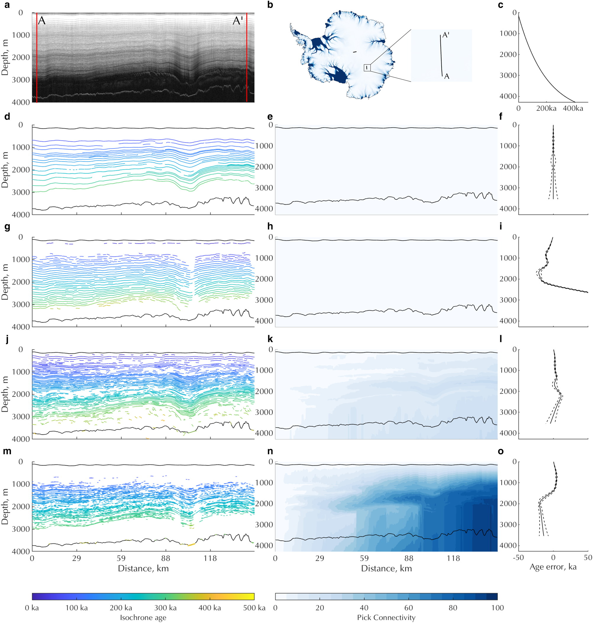
Fig. 1. Comparison of age propagation through auto-tracked isochrones. (a) The raw radar data showing coherent, low-dip layers. (b) Location within Antarctica. (c) Synthetic age–depth relationship applied at location A. (d) Manually-picked reference dataset with (e) isochrone connectivity metric and (f) profile of misfit between reference picks age–depth relationship with uncertainties propagated through the picks. (g) Englacial picks, (h) isochrone-connectivity metric and (i) misfit profile for ARESELP algorithm. (j) Englacial picks, (k) isochrone-connectivity metric and (l) misfit profile for Steger algorithm. (m) Englacial picks, (n) isochrone-connectivity metric and (o) misfit profile for Sobel–Feldman algorithm.
Automated isochrone picking
To our reference radar datasets, we applied three algorithms designed to trace layers automatically, which, for simplicity, we will hereafter term the ARESELP, Steger and Sobel-Feldman algorithms. The Automated Radio-Echo Sounding Englacial Layer-tracing Package (ARESELP) autotracker algorithm was developed by Xiong and others (Reference Xiong, Muller and Carretero2018) to autotrace englacial layers. It uses a continuous wavelet transform (CWT) peak detection algorithm with an assumed Ricker or Morlet wavelet, combined with local Hough transform, to estimate local dip and propagate picks away from peak CWT response (seed) points. Initial tests showed that optimum performance was attained using a Morlet wavelet for the CWT and a block size of 20 pixels, ~50 m (depth) × 1500 m (along track) (assuming v ice = 1.68 × 10⁸ ms−1). We found that the Ricker wavelet applied by Xiong and others (Reference Xiong, Muller and Carretero2018), while suppressing noise in regions of high amplitude stratigraphy, failed to generate picks in lower amplitude regions (e.g.between 90 and 120 km in Fig. 2a).
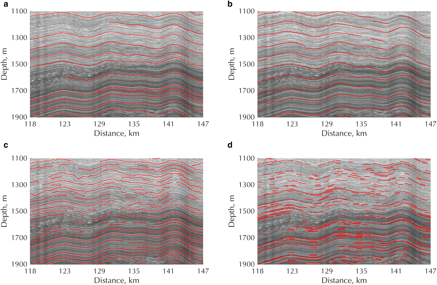
Fig. 2. Detail of each isochrone tracking methodology showing different failure points for each algorithm: (a) Manually-picked reference dataset, (b) ARESELP, (c) Steger filter and (d) Sobel edge detection.
The Steger algorithm is an image-processing technique that follows Ferro and Bruzzone (Reference Ferro and Bruzzone2013) in applying a pre-conditioning block-matching and 3D-filtering process (BM3D filter) (Dabov and others, Reference Dabov, Foi, Katkovnik and Egiazarian2007), followed by a Steger filter ridge detection algorithm (Steger, Reference Steger1998) to enhance and detect englacial layering. In this image-processing context, the ‘ridges’ being detected equate to sets of amplitude peaks in adjacent traces, that represent englacial layers on radargrams. Ferro and Bruzzone (Reference Ferro and Bruzzone2013) applied this technique to extract layering in Mars’ North Polar Ice Cap, but it has not previously been applied to terrestrial radar data. To our reference data, we firstly applied the BM3D filter followed by a stretch to the range [0,255] and application of the Steger ridge detector, filtering to a minimum line length of 50 pixels with an upper and lower threshold of 0.5 and 1, respectively.
Finally, the Sobel–Feldman algorithm is an image-processing edge-detection tool that identifies peak gradients in image brightness (Sobel, Reference Sobel1990). We apply this to the reference data wherein the edges equate to englacial layers, then skeletonise the results to binary images of the detected lines, filtered to remove lines below a minimum size of 50 pixels. This approach is the most simplistic but has the lowest computational cost.
Age–depth relationship propagation
One means of assessing layer-tracking performance is to test the effect each imposes on the propagation of an age–depth relationship through the ice sheet. To gauge this, we deployed a technique similar to MacGregor and others (Reference MacGregor2015), but using a synthetic age–depth profile. We generated a synthetic age–depth relationship using a 1-dimensional Nye model of reflector depth (Nye, Reference Nye1963), as implemented in Leysinger Vieli and others (Reference Leysinger Vieli, Hindmarsh, Siegert and Bo2011) by

where A is the age (years), H, z and b are ice thickness, elevation in the ice column and bed elevation respectively (all in m), and a is the mean accumulation rate (ma−1). We use a representative average accumulation rate of 0.05 ma−1, typical of East Antarctica (e.g. Leysinger Vieli and others, Reference Leysinger Vieli, Siegert and Payne2004), although only the relative amplitudes of errors reported here are of interest and the findings are independent of this rate. This approach makes the assumption of steady-state flow with zero horizontal advection and that all motion is due to basal sliding. We intersect picked isochrones (henceforth referred to as picks) at location A (Fig. 1a) with this age–depth relationship, which can be considered to be similar to a synthetically generated ice core with a known age–depth profile, and assign an age to each pick. We then propagate this age–depth relationship away from A. For each trace, we generate a 1-dimensional age–depth relationship from previously dated picks using a spline interpolation, then assign an age to each un-dated pick with the generated profile. All dated picks are then used to generate the age–depth relationship for the subsequent trace. We then extract the interpolated age–depth profile at a second location A’ (Fig. 1a).
A principal benefit of manual interpretation is the ability to match layers through regions of discontinuous reflectors by recognising patterns or packages of reflections (see, e.g. Karlsson and others, Reference Karlsson2014). For each picked isochrone, we calculate the degree of connectivity between that pick and the starting age–depth profile at A (Fig. 1a). Uninterrupted picks intersecting A are assigned a score of 0 as they present the lowest age uncertainty, assuming the pick is correctly aligned with an isochrone. For each interpolation required to assign a date to a new pick, the connectivity increases by one. The newly dated pick is assigned this score of connectivity, and used for subsequent pick dating. This approach to assessing uncertainty highlights when the interpretation consists of a high number of disconnected isochrones, potentially indicating a high sensitivity to low amplitude signal anomalies.
Englacial dip estimations
To extract dip fields through the reference data, we applied three approaches, which we will hereafter term Panton, ARESP and PWD. The Panton algorithm is described as Step 2 in Panton (Reference Panton2014). We convolve the radar data with a variably-slanted Gaussian kernel to derive the maximum stacking amplitude as a function of dip. The dip field is then filtered to remove noise caused by regions of low signal amplitude, characterised by bands of dip noise between layers, by using an amplitude-weighed spline filter of dip. In Panton (Reference Panton2014), this procedure was presented mainly as pre-processing for englacial-layer tracing, but for this paper, we treat it as one of the direct methods that can be used to extract englacial-layer dip fields across wide swathes of ice sheets.
The Automated Radio Echo Sounding Processing (ARESP) algorithm (Sime and others, Reference Sime, Hindmarsh and Corr2011) firstly applies horizontal stacking to reduce SNR, followed by a binarisation of layers and estimation of local dip of high amplitude signals using a moving window approach.
The plane wave destruction (PWD) algorithm follows Fomel (Reference Fomel2002) in minimising the convolution of a predicted texture with the data to derive local slope. While the Panton and ARESP algorithms have previously been applied widely to radar surveys in Greenland (Sime and others, Reference Sime, Karlsson, Paden and Prasad Gogineni2014; Panton and Karlsson, Reference Panton and Karlsson2015), the PWD method, used routinely in seismic-data processing, is yet to be applied in radioglaciology.
To assess the performance of each algorithm in deriving englacial-layer dip, we use the synthetic age–depth profiles derived previously and consider that the dip of an isochronous reflector will be perpendicular to the angle of maximum gradient. The dip field relative to the surface can therefore be calculated as:

where g x = dA/dx and g y = dA/dy and A(x, y) is the inferred age–depth structure as a function of trace x and depth y. We then propagated a streamline through the data, which represents an integral across the dip field, starting from the location of the synthetic ice core described previously. This highlights the variation in algorithm performance as a function of depth through the radargram.
Results
Isochrone tracking
Figure 1 presents the application of our workflow to our reference data (frames 01_034-036 collected 27/11/2013, Fig. 1a), from East Antarctica's Vostok region, characterised by low dip, continuous reflectors. Parallel results for the more disrupted radar profiles across the Gamburtsev Mountains are presented in Supplementary Figure 1. The numerical results for isochrone tracking algorithms are summarised in Table 1. Englacial layers extracted using ARESELP indicated a high degree of continuity along the section (Fig. 1g). This approach took 4 min 56 s for the example 1 dataset. We extracted 66 individual elements, that in effect pick out most of the englacial layers that we had picked manually, yet the error between reference age–depth profiles at A’ shows a significant deviation of up to − 25 ka in the upper 50% of the ice column with a significant swing to positive errors ~100 ka deeper in the ice column (Figs 1h and i). This error can be traced to breaks in the englacial layers in two ways. Firstly, the algorithm fails to constrain multiple isochrones crossing the amplitude low at 90–120 km, resulting in a region over which the age–depth profile is continued unconstrained in the deeper ice. Secondly, there are additional breaks in layer continuity in the upper layers across which the linking stage of the algorithm has mismatched wavelet peaks between seed points of the layers either side of the breaks.
Table 1. Summary of quantitative assessment of auto-tracking algorithms. N is the number of elements (picks) generated by the algorithm, 〈L〉 is the average length of these picks in number of traces, Median age error and Max age error are the median and maximum difference between interpreted and reference age-depth profiles at A’ (Fig. 1a), and Max Conn. is the maximum value of the connectivity index at A’

The Steger approach shows improvements in some areas (Figs 1j–l) over the ARESELP algorithm. The retrieved age–depth profile shows a maximum error of 10 ka in the deepest regions of ice (Fig. 1l), but there is a greater degree of disconnectivity between A and A’ than for ARESELP (compare Fig. 1l with Fig. 1i). This approach took 48 s per radargram for the BM3D filter, and 23 s for the picking and isochrone linking. We undertook parameter testing to increase the sensitivity to cross the amplitude low at 90–120 km, which led to an increase of picking success, but with an increase of false alarms in the deepest regions of ice. Overall, the Steger algorithm was able to identify 1076 elements in the radargram, compared with 66 from ARESELP, comparatively identifying more isochrones but with more disconnectivity. Up to 35 interpolations were required to constrain the age model throughout (Fig. 1k).
The Sobel–Feldman edge-detection algorithm extracted the highest number of individual elements (3210) throughout the data (Fig. 1m), showing a high sensitivity to low-amplitude signals. This is also highlighted through the degree of connectivity between A and A’, where the maximum number of interpolations reaches 91 at the bed (Fig. 1n). This approach typically took under 1 s for each radargram. This experiment serves to highlight that although a good constraint on age–depth relationship can be achieved using simple edge-detection implementations, the uncertainties associated with propagating age between a high number of low-quality picks suggest that such approaches should be avoided.
Figure 2 shows a detailed sub-set of the data shown in Figure 1 to better highlight the relative strengths and weaknesses of each of the three tracing approaches. The ARESELP algorithm shows the most continuity and smoothest reflector dip throughout the data. In regions of good signal to noise ratio, the Hough transform approach to isochrone linking generally performs well, but dips deviate from the radargram structure for numerous internal layers (e.g. the layer starting at 1550 m depth). There are also numerous picks where the interpretation fails to trace reflector peaks successfully or, more significantly, jumps at a high angle (e.g. depth ≈ 1400 m in Fig. 2b). This can give rise to substantial deviations in the age–depth profile propagated along profiles. This behaviour reflects the results of Figures 1g–i, where the ARESELP algorithm shows that a low degree of connectivity (Fig. 1h) can be achieved between A and A’, but large errors in age–depth relationship are obtained when compared to the reference dataset (Fig. 1i).
The Steger filter gives much more variability and a rougher pick as each ridge is picked independently of the previous one; there is only limited local directional guidance between traces. As such, in regions of strong signal with continuous isochrones the ridge tracking performs well in estimating the dip of structures within the radargram (in general, in the deeper regions of Fig. 2c). Increasing noise levels in the upper region of the figure (depths <1400 m) result in a larger number of noisy, conflicting-dip picks which do not track the radargram structure well. From Figures 1j–l, the general ability of the Steger filter to track the dip of continuous reflectors results in a better age–depth error compared to the ARESELP algorithm, but with more age interpolations required to connect A and A’.
The Sobel–Feldman edge detection algorithm is similar in that the linking is unguided by dip and shows similar variation and susceptibility to the variation of reflection amplitude to the Steger pick. The sensitivity of the Sobel–Feldman technique is higher to low-amplitude signals, resulting in the higher number of picks, but should be noted that despite this, the Sobel–Feldman shows a much lower susceptibility to crossing radargram layers in Figure 2d compared to both the Steger filter and ARESELP algorithms. This results in a much larger number of interpolations required to propagate the age–depth structure, which is reflected in Figure 1n.
Dip estimation techniques
Figure 3 presents englacial-dip fields along profile AA’ derived directly from the manual englacial-layering picking (panel a) then from the three automated approaches. The Panton approach to dip estimation (Fig. 3b) shows a good agreement with the reference dataset. This approach includes a step to remove noise in regions of low amplitudes and applies an interpolation across such regions. There is also little differentiation between noise and englacial-layer dips, such that incorrect dips are propagated across the echo-free zone, shown for example by a reversal of the dip at the deepest regions of ice at ~110 km along the profile and small-scale variations close the lowest streamline in Figure 3b.
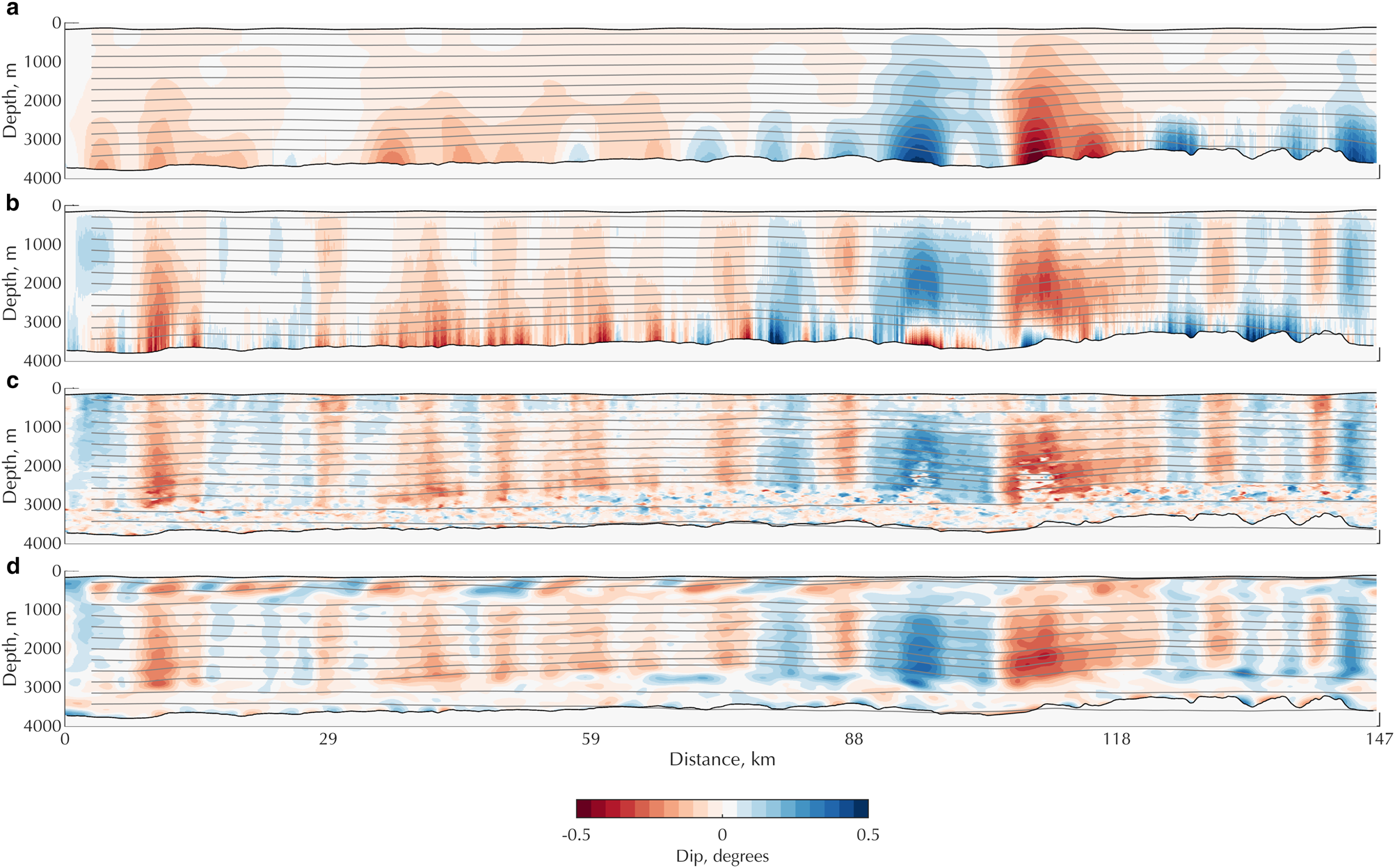
Fig. 3. Propagation of a streamline through dip fields derived from (a) reference picks, (b) Panton slope-extraction step, (c) ARESP and (d) using PWD.
The ARESP approach exhibits higher sensitivity to lower-SNR regions, highlighted in the middle of the ice column at 110 km (Fig. 3c). Beneath the lowest traced englacial layer the average dip is zero, although slight noise in dip amplitude is observed.
Finally, the PWD method yields a higher degree of smoothing than ARESP, and has a flat streamline through the deepest ice. It is, however, sensitive to non-zero dips in the near surface that are not present or detected by the other techniques, and the uppermost streamlines deviate towards the surface as a result.
Discussion
Isochrone tracking intercomparison
Xiong and others (Reference Xiong, Muller and Carretero2018) compared their ARESELP results to the picks from the manually-constrained interpretation of MacGregor and others (Reference MacGregor2015) using a direct overlay of extracted isochrones, which enabled only a limited degree of inter-comparison and quantitative assessment. Ferro and Bruzzone (Reference Ferro and Bruzzone2013) similarly used a manually-picked dataset as a reference against which to compare their application of the Steger algorithm, but further compared their results in terms of false alarms and missed layers to guide optimal parameter selection. Critically, neither of these approaches facilitated quantitative insights into the glaciological implications of incorrect picking in an automated algorithm, which we can gain from the age–depth relationship propagation.
The results of this comparison show that significant errors in age–depth structure can result from isochrone tracking algorithms. On our least complex dataset, the best algorithm resulted in a 11.1 ka error, but with large uncertainties due to the low number of continuous reflections between A and A’. Cavitte and others (Reference Cavitte2016) model the age uncertainty from manual layer tracking as a combination of ice core age uncertainty and the radar range resolution and estimate an upper bound of uncertainty of 3.73 ka. Winter and others (Reference Winter, Steinhage, Creyts, Kleiner and Eisen2019) similarly estimate typical errors <2 ka, but up to 3.7 ka. Hence, none of the isochrone-tracking methods trialled in this study is yet able to rival the accuracy of picking englacial layers manually. However, manual interpretation of multiple layers takes of the order of days per 100 km, especially where the layering structure is disrupted or broken. Expanding this across the Antarctic data record, with ongoing surveys with ever-improving resolution rapidly becomes a considerable effort, which motivates the further development of auto-tracking algorithms.
The approach to age–depth propagation used here comprises a simpler implementation of the effective-strain estimation approach of MacGregor and others (Reference MacGregor2015), giving an interpolated fit rather than a physically-derived age–depth profile between isochrones. We found that due to the noisy and potentially converging layer picks from the automated approaches tested here, effective-strain estimations can be highly variable resulting in rapid deviations away from the expected ages. As algorithms improve, age propagation through a local strain estimation should be used. Despite ours being an approximate approach, it nonetheless gives insights into the performance of age-structure propagation through picked isochrones beyond a direct comparison of picked horizons.
Our approach to age–depth uncertainty using synthetic ice-core connectivity also highlights further issues that may be encountered with auto-tracking techniques. When manual picking is used, isochrones may be tracked across discontinuous regions in the absence of intersections with other interpreted profiles through recognising similar packages of reflections on either side of the noisy region (Cavitte and others, Reference Cavitte2016; Ashmore and others, Reference Ashmore2020), similar to practice in the seismic interpretation workflow (Nanda, Reference Nanda2016). However, none of the automated layer-tracking algorithms investigated here have implementations that allow the recognition, and matching, of similar packages of layers across gaps in the records. Such shortcomings that have challenged wider layer-tracing efforts have indeed been one of the major motivations for developing dip tracking as an alternate approach. Matching layer packages has long been a challenge in the field of automated seismic interpretation, where discontinuities are prevalent as faults. Discontinuities could potentially be overcome using artificial neural networks (Harrigan and others, Reference Harrigan, Kroh, Sandham and Durrani1992) or through global interpretation (Hoyes and Cheret, Reference Hoyes and Cheret2011) but these approaches have yet to be applied to ice-sheet radiostratigraphy.
Future automated interpretation techniques need to target automated linking of interpreted horizons to match disconnected isochronal picks derived from the local peak tracking. The principal issue experienced with implementations tested here relates to trackers deviating from the target reflection. The ARESELP algorithm overcomes this to an extent as a result of the use of a Hough transform, yet still results in errors of age–depth profile as a result of deviations away from the data stratigraphy. Such linking may further be enhanced using correlation or artificial neural network approaches to signal matching, or through tracking along multiple trajectories using a confidence-based metric. The example and approach of age propagation testing presented here could be used to test these approaches.
Isochrone dip estimation
Each of the tested dip-retrieval algorithms worked well in the case of high-amplitude, high-SNR regions of the radargram. Failures occurred at three major locations: the deepest regions of ice with weaker or absent echoes; where englacial layers dip most steeply and SNR drops; and in the near surface. These are each where the signal power drops, or where local amplitudes vary rapidly as in the near surface. To combat this, operational use of algorithms could limit dip estimation to the middle of the ice column, following an approach commonly adopted for estimating layer continuity where the upper and lower 20% of the ice column are not used (Karlsson and others, Reference Karlsson, Rippin, Bingham and Vaughan2012; Bingham and others, Reference Bingham2015). The Panton approach tested here did attempt to remove such low-amplitude regions by removing high spatial-frequency noise, but the drawback of this approach is the interpolation and associated loss of information from regions where dip is high, e.g. in the lower ice. This compares to Holschuh and others (Reference Holschuh, Parizek, Alley and Anandakrishnan2017), who used signal-amplitude thresholding within a moving window to reduce the impact of low-amplitude areas, returning a zero dip field in these regions.
Modern SAR processing of airborne phase-coherent data offers opportunities for direct estimation of englacial-layer dip. Castelletti and others (Reference Castelletti, Schroeder, Mantelli and Hilger2019) presented a process to derive englacial-layer dips using retrieved phase before stacking to undertake in phase-coherent systems to reduce the effects of destructive stacking described in Holschuh and others (Reference Holschuh, Christianson and Anandakrishnan2014). Such an approach shows promising results in retrieving a dip field and enhancing layer coherence from complex data, but has yet to be applied to a larger region of Antarctica to aid a wider interpretation of ice-sheet stratigraphy.
Conclusions
We have undertaken an intercomparison of three isochrone auto-tracking and three englacial-dip estimation algorithms which may be used for wider exploration of the englacial radio-stratigraphic structure of the Antarctic Ice Sheet. We have presented a formal procedure for evaluating these approaches relative to a manually-picked reference dataset to give a reliable indication of the benefits and shortcomings of each isochrone tracking technique. Of the automated isochrone trackers tested here, there is only limited success in linking the age–depth profile between two locations along a relatively simple isochrone geometry. Of the three algorithms tested, the ARESELP procedure (Xiong and others, Reference Xiong, Muller and Carretero2018) is best at retrieving substantial lengths of isochrones, yet can be prone to deviations in dip. While the Steger algorithm (Ferro and Bruzzone, Reference Ferro and Bruzzone2013) shows a greater uncertainty in propagated ages, it shows an improvement in tracking general dip and a lower error in propagated age profile. Supplementing this approach with more advanced pattern-matching using, for example, neural networks to improve isochrone pick continuity is recommended.
The three different approaches to dip estimation that we tested all performed relatively well on our reference datasets, although all are challenged in the deepest ice and at the near-surface. All have the potential for higher performance by adopting improved data preprocessing, application of tapered windows or thresholding (e.g. Holschuh and others, Reference Holschuh, Parizek, Alley and Anandakrishnan2017). Future developments in automated tracking should focus on the ability to automate linking of interpreted isochrones and use a similar approach to age propagation to demonstrate successful implementation. We propose that the methodology developed here, and the two datasets from East Antarctica presented in this study, covering a range of englacial conditions, may be used as a standard validation approach for future algorithm developments.
Author contribution statement
RD, DMS and RGB designed the research. RD performed the analyses at Stanford University with DMS and at the University of Edinburgh with RGB, AC and AG. RD wrote the paper, and all authors contributed edits to the final paper.
Acknowledgments
This paper was stimulated by the AntArchitecture Action Group of the Scientific Committee for Antarctic Research. RD and RGB acknowledge funding from the U.K.'s Natural Environment Research Council via RD's scholarship in the Edinburgh E3 Doctoral Training Partnership (NE/L002558/1) and the Scottish Alliance for Geoscience, Environment and Society (SAGES) via a Postdoctoral Early Career Research Exchange (PECRE) for RD to work with DMS at Stanford University. DMS was partially supported by an NSF CAREER award. We also acknowledge support from the Trans-Antarctic Association (Small Grant TAA-04-19) that allowed RD to present the work at the IGS Radioglaciology Symposium associated with this volume. We acknowledge the use of data and/or data products from CReSIS generated with support from the University of Kansas, NSF grant ANT-0424589, and NASA Operation IceBridge grant NNX16AH54G. We thank Martin Siegert, Hester Jiskoot and one anonymous reviewer for their comments on this paper.
Supplementary material
To view supplementary material for this article, please visit https://doi.org/10.1017/aog.2020.42


 Open access