


1. Introduction
For high-enthalpy flows, e.g. re-entry environments, the requirement to maintain the surface of the vehicle at a temperature much lower than at the boundary layer edge may give rise to the appearance of disturbances travelling at supersonic speeds relative to the free stream, i.e. supersonic modes (Chuvakhov & Fedorov Reference Chuvakhov and Fedorov2016; Mortensen Reference Mortensen2018). Although, initially, the role of the supersonic mode may not have been appreciated as much by the scientific community due to its lower amplification rate compared to the second mode (Mack Reference Mack1987, Reference Mack1990), recently, there has been a renewed interest in studying its characteristics, starting with the work by Bitter & Shepherd (Reference Bitter and Shepherd2015). Knisely & Zhong (Reference Knisely and Zhong2019c) noted that the emergence of the supersonic mode leads to an enlarged unstable region, potentially increasing the overall  $N$-factor. For blunted cones with a low wall-to-free-stream temperature ratio, Mortensen (Reference Mortensen2018) stated that the transition to turbulence is more likely to be caused by the supersonic mode rather than by the second mode for typical re-entry conditions. However, the author also speculated that the supersonic mode, which is distinctly recognisable by its fluctuations emanating above the boundary layer edge into the free stream, may inherently radiate energy away from the boundary layer and, thus, stabilise the boundary layer instability modes.
Although significant work has been carried out to understand the supersonic mode by Zhong's group (Knisely & Zhong Reference Knisely and Zhong2019a,Reference Knisely and Zhongb,Reference Knisely and Zhongc) and others (Salemi & Fasel Reference Salemi and Fasel2018; Zanus et al. Reference Zanus, Knisely, Miró and Pinna2020), the underlying mechanisms associated with the so-observed radiation of sound from the boundary layer has not been comprehended well yet. One of the key questions is if linear stability theory (LST) can be used to predict the evolution of the second mode and the appearance of an acoustic-like beam emanating from the wavepacket as observed in direct numerical simulations (DNS). Tumin (Reference Tumin2020) used an LST-based initial value problem approach assuming parallel flow and demonstrated that neither nonlinear interactions between different modes nor non-parallel effects are needed to generate an acoustic-like beam from the tail of the wavepacket. While this study shows that the acoustic-like beam emanating from a wavepacket can be generated purely linearly and in a parallel flow, it does not explain the observations by Knisely & Zhong (Reference Knisely and Zhong2019a) and Chuvakhov & Fedorov (Reference Chuvakhov and Fedorov2016). Knisely & Zhong (Reference Knisely and Zhong2019a) observed the appearance of acoustic radiation for a boundary layer flow where no unstable supersonic mode was identified with LST and attributed it to nonlinear interaction between the stable supersonic mode ( $F$), the unstable subsonic mode ( $S$) and the slow acoustic ( $SA$) spectrum. Chang, Kline & Li (Reference Chang, Kline and Li2019) hypothesise that synchronisation between the acoustic waves and the instability in the non-parallel boundary layer causes the appearance of the supersonic mode, not a nonlinear modal interaction as reported before.
The current paper, while relevant to the two aforementioned studies, aims at explaining the mismatch in the growth rate predictions observed between DNS and LST, in particular, for the DNS work presented in Chuvakhov & Fedorov (Reference Chuvakhov and Fedorov2016). In addition to locally parallel LST, Chuvakhov & Fedorov (Reference Chuvakhov and Fedorov2016) employed non-parallel stability theory (NLST) and showed that the discrepancy observed in the growth rate is not due to non-parallel effects. Beyond the synchronisation of the second mode with the acoustic spectrum, i.e. phase locking, the role of the continuous acoustic spectrum in the presence of the supersonic modes has not been fully examined. Hence, in this work, biorthogonal decomposition (BOD) is used to explain the roles of the discrete supersonic modes and the continuous acoustic spectrum in the region where so-called spontaneous acoustic emission was observed.
2. Problem set-up and numerical methodology
The Mach  $6$ flat-plate boundary layer flow conditions are identical to those used in Chuvakhov & Fedorov (Reference Chuvakhov and Fedorov2016) with a wall temperature of $T_w=150$ K, and a free-stream temperature of $T_\infty =300$ K. The computational domain spans $x \in [3,18]$ m in the streamwise direction and $y \in [0,2.5]$ m in the wall-normal direction, with $10\,000$ and $500$ grid points, respectively. A similarity profile is prescribed at the inflow of the computational domain, and an outflow buffer is placed at $x=17.8$ m to reduce reflections at the outflow. After obtaining a steady mean flow, the disturbance flow field is computed by solving the linear disturbance equations following the approach in Browne et al. (Reference Browne, Haas, Fasel and Brehm2019). Disturbances are introduced employing volume forcing in $x \in [7,7.03]$ m in the form
 \begin{equation} S(x,y,t) = A \sin\left(\frac{2{\rm \pi}(x-x_o)}{\Delta x_w}\right)\exp\left(-\dfrac{(y-y_o)^2}{\sigma_y}\right)\sin(\omega t), \end{equation}
where disturbances with a frequency of  $F=8.8485\times 10^{-5}$ are introduced to excite second-mode instability waves. The frequency parameter is defined as $F=\omega \mu _\infty /(\rho _\infty U_\infty ^2)$, where $\rho _\infty$, $\mu _\infty$ and $U_\infty$ represent the density, viscosity and mean flow velocity at the free stream, respectively. The frequency considered here corresponds to the lowest-frequency case presented in Chuvakhov & Fedorov (Reference Chuvakhov and Fedorov2016) with the largest region of supersonic mode growth. The LST solver used here assuming parallel flow and the travelling wave ansatz is detailed in Tumin (Reference Tumin2007). The eigenvalues obtained from the stability solvers are the complex wavenumbers, where the negative of the imaginary component of the eigenvalue ( $-\alpha _i$) represents the spatial growth rate. Using the real component of the wavenumber $\alpha _r$ and the circular frequency $\omega$, the non-dimensional phase speed for a two-dimensional disturbance is computed as $c_r = \omega /\alpha _r$. To conduct the BOD, the disturbance flow field is first Fourier-transformed. The BOD solver requires the primitive variables and its derivatives in all three directions for a three-dimensional disturbance. The biorthogonal eigenfunction system (BES) is obtained by solving the direct and adjoint problems; see details in Tumin (Reference Tumin2007) and Hasnine et al. (Reference Hasnine, Russo, Browne, Tumin and Brehm2020).
3. Results and discussion
3.1. Simulated disturbance flow field
Part of the DNS flow field is shown in figure 1(a) in terms of disturbance pressure. The vertical coordinate  $\eta$ is the ratio of wall-normal distance $y$ to the Blasius length scale $H = (\mu _\infty x/\rho _\infty U_\infty )^{0.5}$, where $H$ is computed based on $x=9$ m. The synchronisation of the fast mode $F$ and the slow discrete mode $S$ leads to the appearance of the second mode at around $x=5.8$ m with a typical two-cell structure close to the wall. The phase speed of the second mode decreases as it travels downstream, and, due to the cold wall condition, it approaches the phase speed of the slow acoustic wave, i.e. $c_r=1-1/M_\infty \simeq 0.833$. The occurrence of spontaneous acoustic emission (as referred to by Chuvakhov & Fedorov (Reference Chuvakhov and Fedorov2016)) marks the appearance of the supersonic mode at around $x=9.9$ m, which travels supersonically relative to the free stream. The DNS flow field in figure 1(a) qualitatively resembles the disturbance flow field presented in Chuvakhov & Fedorov (Reference Chuvakhov and Fedorov2016) in terms of the presence of the second mode and the supersonic mode, although the flow visualisation in their paper was provided for a higher frequency, i.e. $F=1.3124\times 10^{-4}$, compared to the case considered here. The lower-frequency case is chosen due to the enlarged supersonic mode region corresponding to this frequency compared to the $F=1.3124\times 10^{-4}$ case.
(a) Disturbance pressure field obtained from DNS and insets showing LST eigenfunctions for the second mode and the supersonic mode. Here  $c_r^-$ and $c_r^+$ correspond to the phase speed of the slow and the fast acoustic waves, respectively, and $c_r^*$ marks the critical layer. (b) Variation of the phase speeds of the fast mode $F$ and the slow mode $S$ along the flat plate showing the regions of the second mode and the supersonic mode.

The insets in figure 1(a) show eigenfunctions at  $x=7.58$ m and $x=10.88$ m, where the second and the supersonic modes are the dominant instability, respectively. The amplitude profiles corresponding to streamwise velocity, pressure and temperature are shown after normalising by the pressure amplitude at the wall. The blue dashed lines identify the relative supersonic regions along with the critical layer. For the second mode, there is only one relative supersonic region close to the wall, bounded by the sonic line $M_r=(U-c_r)M_\infty /\sqrt {T}=-1$, where $U$ and $T$ are the non-dimensional mean flow velocity and temperature, respectively. However, for the supersonic mode, in addition to the one present near the flat-plate surface, there appears another relative supersonic region outside the critical layer with $M_r\geq 1$. Another well-known feature of the supersonic mode is that the eigenfunctions corresponding to this mode decay very slowly outside the boundary layer compared to the second mode, which can also be seen in figure 1(a).
3.2. Comparison of DNS data with LST and BOD results
The eigenvalue spectra obtained from the spatial LST at three different locations along the flat plate are plotted in the complex wavenumber plane in figure 2(a). The fast ( $FA$) and slow ( $SA$) acoustic branches are identified along with the slow discrete mode $S$ and the fast discrete modes $F^+_1$ and $F^-_1$. The second mode $F^+_1$ appears as the dominant instability at the first location $x=7.58$ m, whereas the supersonic mode $F^+_1$ emerges as the most unstable mode at the other two locations. The trajectory of the fast mode $F_1$ is shown in the complex phase plane in figure 2(b) at three different wall-to-free-stream temperature ratios. A jump in the imaginary part of the eigenvalue is observed near the entropy/vorticity branch marked by the black dashed line at $c_r=1$. At this location of the flat plate, the presence of non-parallel effects allows for modal interaction between the discrete mode $F_1$ and the vorticity/entropy branch and therefore provides a receptivity mechanism. It also provides the initial amplitude of the $F_1^+$ mode before it synchronises with the slow mode $S$ further downstream ( $c_r\approx 0.945$) to generate the second mode. A two-mode approach is required to describe the inter-modal exchange between the synchronising discrete modes $F_1^+$ and $S$ near the vicinity of the branch point as detailed in Fedorov & Khokhlov (Reference Fedorov and Khokhlov2001). A reduction in the wall temperature leads to a lower amplification of the second mode as can be seen from figure 2(b).
(a) Eigenspectrum in the complex wavenumber plane showing the discrete modes along with the slow and the fast continuous spectra. (b) Trajectory of the first fast mode in the complex phase plane at varying wall-to-free-stream temperature ratios  ${T_w}/{T_\infty } = 0.5$, 0.25 and 0.15. (c) Variation of phase speed of the slow mode and the fast mode along the flat plate computed using LST and DNS.

The synchronisation between the second mode  $F_1^+$ and the $SA$ branch, which is marked by the second black dashed line at $c_r\approx 0.83$, is not similar to that between the fast mode $F_1$ and the entropy/vorticity branch, as it does not lead to coalescence of the eigenvalues. When the supersonic mode appears, the second mode $F_1^+$ is not swallowed by the acoustic branch; however, another discrete mode $F_1^-$ emerges from the continuous branch, with similar phase speed but with an opposite sign of the growth rate, as can be seen from figure 2(a). The non-parallel nature of the boundary layer at the synchronisation point provides a mechanism for inter-modal exchange, which may serve as an explanation for the initial amplitudes in $SA$ and $F_1^-$. As the wall-to-free-stream temperature ratio is reduced from $0.5$ to $0.25$, the amplification rate of the supersonic mode increases slightly; however, a further reduction in the temperature ratio leads to a decrease in the growth rate.
The blue line in figure 2(c) corresponds to the phase speed computed using the wall-pressure data obtained after applying a fast Fourier transform (FFT) to the DNS data. The streamwise location where the supersonic mode appears in the flow field with  $c^-_r = 1-1/M_\infty$ is in close agreement between LST and DNS, similar to what was reported in Chuvakhov & Fedorov (Reference Chuvakhov and Fedorov2016).
Next, the amplitude development of surface pressure extracted from DNS is compared to LST predictions of the  $F^+_1$ mode in figure 3(a). While both LST and FFT show a very similar trend, i.e. an increase in the amplitude of wall pressure in the streamwise direction, some offset in the amplitude curves is apparent. The projected data on the $F^+_1$ mode computed using BOD closely follow the FFT signal in the second-mode region, which implies that the DNS flow field is primarily dominated by the $F^+_1$ mode. In the supersonic mode region, however, there is a slight mismatch in the two datasets near the black dashed-dotted line. Further downstream, good agreement between the FFT and the projected data is again observed. On the other hand, different trends are noticed for the LST and the projected data for the other supersonic mode $F^-_1$, which appears alongside the supersonic mode $F^+_1$ at the branching point. Although LST predicts that the $F^-_1$ mode should be damped in the streamwise direction, the projected data show an increase in the amplitude. To the best of our knowledge, this discrepancy has not been reported in the literature before, and it is not clear at this point how the presence of this mode, which would otherwise be strongly damped, affects the overall characteristics of the disturbance flow field.
Comparison of (a) wall-pressure amplitudes and (b) growth rates obtained from LST, BOD and the FFT of the DNS data at  $F = 8.8485\times 10^{-5}$.

Figure 3(b) provides the growth rate (the rate of amplitude change based on the Fourier-transformed DNS data is loosely referred to as amplification or growth rate,  $-\alpha _i={\rm d}(|p'_w|)/{{\rm d} x}$)) computed using the wall-pressure amplitude presented in figure 3(a). The growth rate of the $F^+_1$ mode obtained from LST closely follows the FFT signal in the second-mode region. As opposed to the similarity profile used in Chuvakhov & Fedorov (Reference Chuvakhov and Fedorov2016), this work makes use of the numerical mean flow; therefore, the LST growth rate is not shifted to the left of the FFT data as they had noted in their work. Compared to the LST prediction, the data projected on $F^+_1$ provide a closer match with the DNS growth rate in the second-mode region. Although at a different frequency, Chuvakhov & Fedorov (Reference Chuvakhov and Fedorov2016) also reported a similar mismatch of the LST and FFT growth rates in the regions of flow where the supersonic mode is the dominant instability. Based on their NLST study, the disagreement in the growth rate data cannot be explained by non-parallel effects as suggested in Knisely & Zhong (Reference Knisely and Zhong2019c).
The location of maximum growth rate obtained from the projected data in the supersonic mode region is shifted to an upstream location compared to the FFT data. The projected data show a dip ahead of the maximum growth rate location similar to that predicted by NLST in Chuvakhov & Fedorov (Reference Chuvakhov and Fedorov2016). While the projected growth rate deviates from the FFT data, it aligns with the LST data directly after the maximum amplification location. The mismatch of the projected and the FFT growth rates in the supersonic mode region implies that the disturbance flow characteristics of the DNS flow field are not entirely dictated by the (single) most unstable mode  $F^+_1$ as predicted by LST (as observed in the second-mode region). To investigate the behaviour of the other supersonic mode $F^-_1$ and its contribution to the disturbance flow field, we also computed the amplification rate corresponding to this mode using the projected wall-pressure amplitude. Although LST predicts that $F^-_1$ is damped, this mode in actuality experiences amplification and even locally exceeds the growth rate of the $F^+_1$ mode when it first appears. Hence, based on the results above, it appears that the contribution of the $F^-_1$ mode cannot be neglected, and the role of this mode on the behaviour of the disturbance flow field will be further explored in the next section.
3.3. On the relative importance of the discrete modes and the continuous spectrum
To evaluate the contributions of the discrete modes and the continuous spectrum, BOD is applied to the FFT data. The first location selected for comparison is  $x=10.22$ m, which showed the largest difference in growth rate between LST and FFT in figure 3(b). First, the projection onto the two supersonic modes $F^+_1$ and $F^-_1$ is considered, and in figure 4(a) the real part of the disturbance temperature is plotted versus the non-dimensional wall-normal distance. Both modes show typical supersonic mode behaviour, with large variations of temperature near the wall and close to the critical layer, and continuous oscillations outside the boundary layer until the viscous dissipation attenuates the oscillations.
(a) Comparison of the real component of disturbance temperature obtained from BOD with FFT data at  $x=10.22$ m. (b) Variation of the projection coefficient for the $SA$ branch as a function of the continuous spectrum parameter $k$.
$k$.

Although the temperature profile corresponding to the  $F^+_1$ mode closely follows the FFT data, the contribution from the other supersonic mode $F^-_1$ is significant and cannot be neglected. It is to be noted that the BES provides a complete set of eigenfunctions, as discussed in Tumin (Reference Tumin2007). When both the discrete modes are superimposed, the resulting disturbance temperature profile, however, overpredicts the FFT signal considerably. Therefore, there must be some other mode or combinations of modes present cancelling out the contribution from the $F^-_1$ mode. To examine that, the disturbance flow field is projected onto the other two discrete modes $S$ and $F^-_2$ appearing in the eigenspectrum in figure 2(a); however, both modes provide negligible contributions to the disturbance flow field. Therefore, it must be the continuous branches that provide similar contributions as the discrete supersonic mode $F^-_1$. Hence, next, the disturbance flow field is projected onto the two (fast and slow) acoustic branches, in addition to the vorticity and the entropy branches.
For the projection onto the continuous branch, the spectrum is approximated by superimposing a finite number of modes with different wavenumbers all belonging to the same continuous branch. The contribution from the continuous spectrum changes as the phase speed of the supersonic mode decreases in the downstream direction. To illustrate this, the disturbance flow field is projected onto a subset of modes belonging to the  $SA$ branch in figure 4(b). A key characteristic of the continuous modes is that they oscillate outside of the boundary layer proportional to $\exp (-{\rm i}ky)$, where the continuous spectrum parameter $k$ can be interpreted as a wall-normal wavenumber. In figure 4(b), the projection coefficient $C_k$ is plotted as a function of the continuous spectrum parameter $k$ for multiple locations along the flat plate. Within the context of the BES, the eigenfunctions were normalised in such a way that the pressure reaches an amplitude of one at the wall. Hence, $C_k$ essentially provides a measure for the contribution of the surface pressure amplitude between the projected data for each mode $k$ and the FFT data. For each of the $C_k$ curves, a narrow peak can be observed, implying that only a small range of modes from the continuous branch contribute to the overall disturbance flow field at a fixed location. In the downstream direction, the $C_k$ curves shift to the right and become more asymmetrical, with an increased contribution from the higher wavenumbers.
The temperature profile corresponding to the  $SA$ branch at $x=10.22$ m in figure 4(a) is obtained by taking a weighted average of the profiles computed for a range of $k \in [0.001,5]$ with $\Delta k = 0.001$. The fast acoustic, entropy and vorticity branches do not contribute significantly, hence, their profiles are not included in figure 4(a). The projected temperature profile of the $SA$ branch shows an exact opposite phase to that of the $F^-_1$ mode. When superimposing the two supersonic discrete modes $F^+_1$ and $F^-_1$ with the $SA$ branch, the resulting profile more closely aligns with the FFT signal. While the differences are very subtle within the boundary layer, the relevance of the linearly decaying (based on LST) supersonic mode $F^-_1$ and the $SA$ branch will be further highlighted in the following discussion. It should be noted that, in the second-mode instability region, only the (single) $F^+_1$ mode is sufficient to reconstruct the FFT signal, similar to the growth rate data, which can be perfectly matched with LST.
To further investigate the role of the  $SA$ branch and the $F^-_1$ mode for reconstructing the disturbance flow field, the projected amplitude profiles of pressure and the total disturbance energy, $E'=\tfrac {1}{2}(\rho u_i^\ast u'_i + TR \rho ^\ast \rho '/\rho + \rho C_v T^\ast T'/T)$, computed using Mack's energy norm, are shown at $x=10.88$ m in figure 5. This location corresponds to the maximum amplification of the supersonic mode as predicted by DNS. As shown in figures 5(a) and 5(b), the supersonic mode $F^+_1$ closely follows the FFT signal inside the boundary layer, with small differences noticed around the peaks (see the inset in figure 5b) eliminated by the superposition of the $F^-_1$ mode and the $SA$ branch. A closer examination of the different datasets reveals significant differences in the behaviour of the FFT signal and the supersonic mode $F^+_1$ outside of the boundary layer in figure 5(c). For a wall-normal distance greater than $\eta =50$, the oscillations in the FFT signal cease to exist. However, the two discrete modes continue to display oscillations due to the modulation caused by the $SA$ spectrum. While none of the discrete modes nor the continuous spectrum are able to replicate the FFT variation outside the boundary layer, the superimposed data computed from the $F^+_1$, $F^-_1$ modes and the $SA$ branch reconstruct the DNS data perfectly.
Variation of (a) amplitude of projected disturbance pressure and (b) total disturbance energy computed using Mack's energy norm along the boundary layer at  $x=10.88$ m. (c) The projected amplitude profile of $p^\prime$ outside the boundary layer.

While the completeness of the eigensystem for disturbance flow reconstruction has been discussed for model problems in Tumin, Wang & Zhong (Reference Tumin, Wang and Zhong2007) and Tumin (Reference Tumin2007), full reconstruction of the disturbance flow field, including the discrete modes and the continuous spectrum, has rarely been demonstrated in the literature. In Knisely & Zhong (Reference Knisely and Zhong2019c), the deviation of the LST eigenfunctions from the DNS data was attributed to the modulation of the disturbance by the  $SA$ spectrum; however, it was not shown explicitly. To the best of our knowledge, the role of the $F^-_1$ mode and the $SA$ branch for reconstructing the disturbance flow field has not been demonstrated in the literature before.
The relative contributions of the two discrete modes  $F^+_1$ and $F^-_1$ and the $SA$ spectrum can also be evaluated by computing the projection coefficient at different locations along the flat plate. For the $SA$ branch, the projection coefficient is evaluated in integral form as $|C|=\int _{k_l}^{k_u} C_k\,{\rm d}k$, where the variation of $C_k$ is shown in figure 4(b) for a range of the slow continuous spectrum parameter $k\in [k_l,k_u]$. The variation of $|C|$ in figure 6(a) shows that the maximum contribution to the disturbance flow stems from either the second mode or the supersonic mode $F^+_1$, with a projection coefficient close to $1$. However, when the other supersonic mode $F^-_1$ appears in the flow, it also provides a significant contribution to the disturbance flow field, with a projection coefficient ranging from $0.4$ to $0.52$. The projection coefficient for the $SA$ branch is shown only in the supersonic mode region, and it follows a similar trend as that of the discrete mode $F^-_1$. The interpretation of this result is obscured by the way the reconstruction of the disturbance flow field is performed through a superposition of different modal contributions.
Variation of (a) the projection coefficient and (b) the growth rate along the flat plate computed for the two supersonic modes  $F^+_1$ and $F^-_1$ along with the $SA$ branch.

Finally, to scrutinise the discrepancy observed between the projected and the FFT growth rate data in figure 3(b), these results are reconsidered in the supersonic mode region, employing the findings from the previous discussion. In addition to the two discrete supersonic modes, the growth rate derived from the wall-pressure distribution of the  $SA$ spectrum is also presented in figure 6(b). Since the $F^-_1$ mode emerges from the $SA$ branch as a result of the synchronisation of the $SA$ branch with the second mode, it has a similar growth rate as that of the $SA$ branch at the starting location ( $x=10.132$ m). Initially, the $F^-_1$ mode and the $SA$ branch even display a higher amplification compared to the $F^+_1$ mode. The excitation of the discrete mode $F_1^-$ and the slow continuous acoustic branch is associated with the inter-modal energy exchange between these two and the unstable supersonic mode $F_1^+$. Since none of the projected data are able to match the FFT data alone, the growth rate is computed based on the wall-pressure amplitude obtained from the superposition of the two supersonic modes and the $SA$ branch. As expected from the close agreement in the amplitude curves observed in figure 5, the combined data reproduce the DNS growth rate exceedingly well. It appears that, in particular, the disturbance flow field outside of the boundary layer, often referred to as an acoustic radiation pattern, is a consequence of a multi-modal interaction between the two supersonic discrete modes and the continuous $SA$ spectrum. To correctly predict the amplitude development (and, thus, the amplification rates) of the disturbance flow field, this interaction needs to be accounted for by superimposing the two discrete supersonic modes with the $SA$ spectrum.
Tumin (Reference Tumin2020) and Chuvakhov & Fedorov (Reference Chuvakhov and Fedorov2016) reported that the supersonic mode  $F^+_1$ emits energy away from the boundary layer, as it leads to a negative outgoing energy flux, i.e. Re $(\hat {p}\hat {v}^*) >0$, where $\hat {p}$ and $\hat {v}^*$ represent the eigenfunctions of pressure and the complex conjugate of the wall-normal velocity, respectively. This observation could be confirmed for $F^+_1$ in figure 7(a); however, in the current study, the $SA$ branch also satisfied this condition for $\eta >30$, implying that it also emits energy away from the boundary layer. The energy flux $\hat {p}\hat {v}^*$ redistributes energy (assuming no disturbance energy is introduced at the wall) but does not provide a mechanism for disturbance energy generation.
(a) Variation of the real component of pressure work along the boundary layer at  $x=10.88$ m. (b) Rate of change of total disturbance energy for the supersonic mode computed at $x=10.88$ m compared with the second mode $F^+_1$ at $x=9$ m.

Figure 7(b) plots the rate of change of total disturbance energy ( ${\rm RTE}=- \alpha _{i} U \hat {E}$) along the wall-normal direction at $x=10.88$ m, where $\hat {E}$ is computed based on the Mack's energy norm using the amplitude distributions. The RTE profile connects amplitude distributions and growth rate as well as localises where energy is being generated. The growth rate value used to compute the rate of change of total perturbation energy is obtained from figure 6(b). The disturbance energy rapidly decays outside the boundary layer for the second mode computed at $x=9$ m, whereas a small fraction of the disturbance energy is still available in the free stream for the supersonic mode at $x=10.88$ m. While, inside the boundary layer, the mechanism of disturbance energy generation appear to be governed by the $F_1^+$ mode, outside the boundary layer, a superposition of $F^+_1$, $F^-_1$ and $SA$ is needed to capture this mechanism. When the contributions of all three modes are considered simultaneously, the energy transfer in the free stream decreases at a much faster rate (similar to the FFT rate) compared to the individual predictions.
3.4. Physical mechanism leading to mode coupling
To investigate the physical mechanisms that lead to the coupling between the two supersonic modes,  $F_1^\pm$, and the slow continuous spectrum, $SA$, we performed two additional disturbance simulations assuming some type of parallel flow assumption. In the first simulation, we simply dropped all terms that contained streamwise gradients of the mean flow, and the wall-normal velocity was set to zero. For this simulation, we employed a different version of the disturbance flow solver based on a flux Jacobian-based formulation (Browne et al. Reference Browne, Haas, Fasel and Brehm2019), which allows us to drop the relevant terms in the governing equations. In the second simulation, the same mean flow profile corresponding to the boundary layer state at $x=10.22$ m with zero wall-normal velocity is applied over the entire computational domain. The main difference between the two simulations is that, in the first simulation, the dispersion relationship is changing in the streamwise direction, which is still allowing for mode coupling and is particularly important when a bifurcation occurs. A comparison of the growth rates for the different simulation results is shown in figure 8(a). The growth rates for the first disturbance simulation are indistinguishable from the non-parallel flow simulation results (therefore, not shown) and mode coupling is still present.
(a) Comparison of the growth rate obtained using a non-parallel mean flow versus a parallel mean flow. (b) Comparison of the amplification rate obtained by simulating the linear disturbance equations (LDE) with the nonlinear disturbance equations (NLDE).

The growth rates for the second simulation assuming a parallel mean flow are shown as a blue line in figure 8(a). As the boundary layer thickness is constant in the streamwise direction, the growth rate is constant in the entire domain. The growth rate perfectly matches the LST results at  $x=10.22$ m, where the largest difference with the non-parallel flow simulation was observed. This simulation demonstrates that, when assuming a perfectly parallel mean flow, there is no disagreement between the disturbance flow simulation results and LST. Simply applying the ‘parallel-flow’ assumptions by setting the wall-normal velocity to zero and enforcing that all mean flow derivatives with respect to the streamwise position are zero as in the first disturbance flow simulation does not suffice to eliminate all non-parallel flow effects. It can be concluded that the mode coupling between $F_1^\pm$ and $SA$ is a consequence of the dispersion relation changing in the streamwise direction in the presence of a growing boundary layer.
Moreover, it should be noted that, although Chuvakhov & Fedorov (Reference Chuvakhov and Fedorov2016) employed a non-parallel stability theory (NLST) analysis to try and match the growth rates in the DNS, they did not consider the coupling of the two supersonic modes,  $F_1^\pm$, with the slow acoustic continuous spectrum. The non-parallel effects that are responsible for the mode coupling were not captured in the NLST analysis by Chuvakhov & Fedorov (Reference Chuvakhov and Fedorov2016) because they only considered non-parallel effects on individual modes. Therefore, they did not observe a match of the DNS and NLST growth rate in the supersonic mode region.
To examine if the nonlinear nature of the governing equations affects the mode coupling, we computed the disturbance flow field by solving the nonlinear disturbance equations (Browne et al. Reference Browne, Haas, Fasel and Brehm2022), which does not neglect the nonlinear terms in the disturbance flow equation. The disturbance amplitude was chosen small enough such that the maximum pressure amplitude observed in the entire computational domain did not exceed 1 % of the free-stream pressure value. The growth rates based on the wall-pressure amplitude for the linear and nonlinear simulations are shown in figure 8(b) and they are in agreement. Therefore, it can be concluded that the mode coupling is not affected by any possible nonlinear effects. We also did not observe any effects of the domain boundary treatment on the coupling between various modes, as the domain in the wall-normal direction was chosen large enough and the disturbances at the domain boundary are sufficiently small.
4. Conclusion
The stability characteristics of a Mach  $6$ flat-plate boundary flow were investigated employing DNS, BOD and LST. The cold-wall boundary condition ( $T_w=0.5T_\infty$) leads to the appearance of supersonic modes in addition to the second mode, which is the dominant instability mode in the flow field. While the appearance of the supersonic mode has been reported in the literature a few decades ago, the disturbance flow characteristics are not fully understood, in particular, how LST can be used to reconstruct the spatio-temporal evolution of the disturbance flow field. The present results show that, in the region where the second mode is the dominant instability, both the projected data on the $F_1^+$ mode and the LST data match the amplitude distribution and the amplification rates extracted from the DNS. Assuming that a single instability mechanism is present (or is the overwhelming instability mechanism), this result confirms what has been known for a long time, namely that a single mode captures the characteristics of the disturbance flow field far enough downstream of the forcing slot used in the DNS.
The current analysis shows, however, that using a single amplified mode  $F_1^+$ is not sufficient to reconstruct the disturbance flow field in the supersonic mode dominant region. While the current finding has been discussed in prior works, it has never been properly demonstrated by projecting the solution on the modes of the LST eigenspectrum. In the supersonic mode region, notable differences were observed for the amplification rates obtained from LST, projection on the $F_1^+$ mode, and derived wall-pressure DNS data. When including the contributions from the $F_1^-$ mode and the $SA$ spectrum, the amplitude profiles and the growth rates could be perfectly matched with the DNS data. Inside the boundary layer, the amplitude distributions from the DNS and the projected profiles of the $F_1^+$ mode were already in relatively close agreement, while including the $F_1^-$ mode and $SA$ branch in the reconstruction led to even better agreement, especially around the peaks. It was also noted that the disturbance flow field, in particular, above the boundary layer edge, could not be fully reconstructed without including the supersonic discrete mode $F_1^-$ and the SA spectrum (see figure 9). The coupling of the modes in the supersonic mode region can be attributed to the non-parallel effects, and the effects of nonlinearity of the governing equations was found to be negligible. Finally, the rate of change of total disturbance energy was evaluated, which combines amplitude distributions and amplification rates and can be used to localise the disturbance energy generation. The results for the energy transfer term sums up the key finding that the contributions from $F_1^+$, $F_1^-$ and $SA$ are vital to explain the behaviour of the disturbance flow field in terms of amplitude distributions and amplification rates in the supersonic mode region.
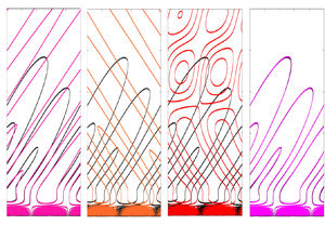
Contours of disturbance pressure obtained from BOD corresponding to the discrete supersonic modes (a)  $F_1^+$ and (b) $F_1^-$; and (c) the slow continuous spectrum $SA$ at $x=10.88$ m. (d) Contours of disturbance pressure obtained from DNS. (e–h) Pressure flow field reconstructed using only the (e) $F_1^+$ mode, ( f) $F_1^-$ mode and (g) $SA$; and (h) superposition of supersonic modes $F_1^+$, $F_1^-$ and $SA$ compared with the DNS pressure data on the background with black contours.

Acknowledgements
We acknowledge the reviewers’ suggestions to further clarify the mode coupling, which added significant value to our manuscript.
Funding
We gratefully acknowledge funding by NASA KY EPSCoR RA Award no. 80NSSC19M0144 with E. Stern as the technical monitor as well as Professor A. Tumin for providing the LST solvers and many fruitful discussions.
Declaration of interests
The authors report no conflict of interest.


 Open access