


1. Introduction
Buoyancy-driven flows in porous media resulting from the injection of fluid of different density to the original reservoir fluid have been studied in some detail owing to their importance for geothermal power production, carbon capture and storage and enhanced oil recovery, for example. The initial models of gravity-driven flow in a porous medium by Barenblatt (Reference Barenblatt1996) and Huppert & Woods (Reference Huppert and Woods1995) established some simple similarity solutions for two-dimensional gravity currents resulting from steady injection, and tested these models with analogue laboratory experiments in isotropic porous media. These models were based on the assumption that the vertical pressure gradient is everywhere hydrostatic and that the flow becomes long and thin, so that the predominantly horizontal flow is driven by the horizontal pressure gradient associated with variations in the thickness of the current. The solution takes the form
 \begin{equation} h/L = ({t}/{\tau})^{1/3} f[(x/L)(t/\tau)^{{-}2/3}], \end{equation}
where  $L=Q_x\mu /k\Delta \rho g$ and $\tau =Q_x(\mu /k\Delta \rho g)^2$ are dimensional length and time scalings, given in terms of the input flow rate per unit length, $Q_x$, the permeability, $k$ (assumed isotropic), the density difference between the two fluids, $\Delta \rho$, and the viscosity of the injected fluid, $\mu$ (Huppert & Woods Reference Huppert and Woods1995). If one extends the analysis to account for different permeabilities in the horizontal and vertical directions, $k_H$ and $k_V$, the assumption of hydrostatic pressure in the flow means that the vertical permeability does not feature in the solution, which is the same as for the isotropic case. This is curious since the vertical permeability of the porous medium may be much smaller than the horizontal permeability owing to the original geological processes of formation and compaction of the medium (Corbett & Jensen Reference Corbett and Jensen1992; Martinius et al. Reference Martinius, Ringrose, Næss, Wen and Hentz1999; Woods Reference Woods2015). The key to this apparent paradox is to assess the vertical pressure gradient required to drive the vertical flow which is implicit in the gravity current solution. With a very small vertical permeability, this pressure gradient scales as
 \begin{equation} \frac{\partial p}{\partial z}\sim \frac{\mu}{k_V} \frac{\partial h}{\partial t} \sim \frac{\mu L}{\tau^{1/3}t^{2/3} k_V}.\end{equation}
For the solution to be valid we require that (1.2) is small compared with the corresponding hydrostatic pressure gradient
 \begin{equation} \frac{\partial p}{\partial z}\sim {\Delta \rho g}. \end{equation}
This requires that
 \begin{equation} t/\tau\gg \left({k_H}/{k_V}\right)^{3/2}, \end{equation}
and we see the role of the vertical permeability in determining the time at which the flow adjusts to the similarity solution. It is worth noting that this result provides an extension of the analysis presented by Huppert & Pegler (Reference Huppert and Pegler2022) who considered the early-time pressure solution in isotropic media.
For radial injection from a point source, the situation is more complex. In the classical similarity solution (Lyle et al. Reference Lyle, Huppert, Hallworth, Bickle and Chadwick2005) there is a singularity in the calculated depth of the current at the origin. However, this result is unphysical, and in order that the flow remains of finite depth at the origin there is a near-origin adjustment zone for all time. Inclusion of this near-origin adjustment zone leads to a different set of scaling laws and a new solution for the current that is influenced by  $k_V$ for all time. In this study we address these details using a theoretical analysis in conjunction with numerical simulations, and we show the analysis is consistent with a series of new laboratory experiments. Our study goes beyond that of Huppert & Pegler (Reference Huppert and Pegler2022), where it was assumed that the pressure-driven flow simply adjusts to the classical similarity solution.
We consider the application of our results to the case of CO $_2$ sequestration in porous geological reservoirs (Bickle et al. Reference Bickle, Chadwick, Huppert, Hallworth and Lyle2007; Szulczewski et al. Reference Szulczewski, MacMinn, Herzog and Juanes2012; Huppert & Neufeld Reference Huppert and Neufeld2014). During the injection of CO $_2$ in such scenarios, a buoyant plume forms within the brine-filled reservoir and rises upwards, spreading out under an impermeable cap rock as a gravity current. There has been an extensive literature on the fluid dynamics of such flows, including studies on the transition to self-similarity in confined aquifers (Hesse et al. Reference Hesse, Tchelepi, Cantwel and Orr2007), multiphase phenomena and relative permeability (Golding et al. Reference Golding, Neufeld, Hesse and Huppert2011; Krevor et al. Reference Krevor, Pini, Zuo and Benson2012; Boon & Benson Reference Boon and Benson2021), residual trapping and dissolution of the CO $_2$ in the brine (Hesse, Orr & Tchelepi Reference Hesse, Orr and Tchelepi2008; MacMinn, Szulczewski & Juanes Reference MacMinn, Szulczewski and Juanes2011) and the effects of geological heterogeneities (Jackson & Krevor Reference Jackson and Krevor2020; Benham, Bickle & Neufeld Reference Benham, Bickle and Neufeld2021b). In the present study we illustrate how anisotropy of the porous medium leads to the ratio $k_V/k_H$ influencing the dispersal of the CO $_2$ at all times, in contrast to the classical gravity current solution. Furthermore, we show that for typical injection rates the transition in flow regime from a pressure-dominated flow to a gravity-dominated flow may occur once the flow has reached depths of 10–1000 m at time scales of 1–10 years, depending on the value of $k_V/k_H$. This suggests that the initial pressure-driven flow persists for a significant period of the injection, and in some cases the flow may never become gravity-driven over the time and length scales relevant to those sites.
The structure of the paper is laid out as follows. Section 2 addresses the flow scenario, treated analytically at early and late times, and comparisons are made with both numerical simulations and porous bead experiments. Section 3 applies the results to the context of carbon sequestration, calculating the criteria for whether a storage reservoir is in a pressure- or gravity-driven regime, and § 4 closes with a discussion of these results.
2. Axisymmetric injection into anisotropic porous media
2.1. A note on anisotropic permeability
Before discussing the flow scenario, we first briefly discuss the geological context of anisotropy in porous media. In subsurface geological reservoirs it is common for the permeability of rocks to differ significantly depending on the direction of the flow (Corbett & Jensen Reference Corbett and Jensen1992; Martinius et al. Reference Martinius, Ringrose, Næss, Wen and Hentz1999). This may result from post-depositional compaction of the formation or from the deposition of successive layers of fine and coarse material. Hence, the permeability field is sometimes written as a three-dimensional diagonal matrix,  $\boldsymbol {k}=\mathrm {Diag}(k_x,k_y,k_z)$, or equivalently in a different basis depending on the direction of compaction (e.g. see studies on cross-bedding Woods Reference Woods2015).
We account for such situations, but we restrict our attention to the case where the compaction is aligned with the vertical coordinate, and hence the permeability is reduced to horizontal and vertical variation only,  $(k_x,k_y,k_z)=(k_H,k_H,k_V)$, where $k_H$ and $k_V$ are constants. Hence, the anisotropy is characterised by the single dimensionless parameter
 \begin{equation} \gamma=k_H/k_V. \end{equation}
This formulation is relevant either for flow through a single thick sedimentary layer that has been compacted vertically, resulting in a binary permeability field, or for flow through a system of many horizontal sedimentary layers, in which the values  $k_H$, $k_V$, can be interpreted as effective permeabilities (Cardwell & Parsons Reference Cardwell and Parsons1945; Kumar et al. Reference Kumar, Farmer, Jerauld and Li1997; Woods Reference Woods2015). For example, in the latter scenario, if the layers vary between permeabilities $k_1$ and $k_2$ over alternating layer widths $d_1$ and $d_2$, then the effective permeability values are given by the arithmetic and harmonic mean values
 \begin{equation} k_H\approx \frac{d_1 k_1 +d_2k_2}{d_1+d_2},\quad k_V\approx \frac{d_1+d_2}{d_1/k_1+d_2/ k_2}. \end{equation}
This tends to be a good approximation as long as the depth of the flow is much larger than the widths of the layers  $d_1,d_2$. Hence, in this system of horizontal sedimentary layers the anisotropy is always such that $\gamma \geq 1$. In fact, for many geological systems the horizontal and vertical permeability have been observed to differ by several orders of magnitude (Martinius et al. Reference Martinius, Ringrose, Næss, Wen and Hentz1999), resulting in anisotropy values as large as $\gamma ={O}(10^4)$.
2.2. The flow scenario at early times and subsequent transition behaviour
Next, we move on to describe the flow scenario we consider, and describe how this evolves at early times, before the effects of gravity become significant. For the isotropic case, as discussed by Huppert & Pegler (Reference Huppert and Pegler2022), the constant input of fluid from a point source results in the current expanding in the shape of a self-similar hemisphere at early times. The radial and vertical extent of the current are equal and grow like the cube root of time. The flow transitions to a gravity-driven regime once the weight of the fluid dominates over the injection pressure. In the following analysis, we extend this early-time analysis to the case of injection into an anisotropic medium, demonstrating how the anisotropy  $\gamma$ affects both the early-time dynamics and the transition behaviour.
We consider the constant axisymmetric injection of fluid (at flow rate  $Q$) into a porous medium with anisotropy $\gamma$ and porosity $\phi$, bounded from below by an impermeable substrate, as illustrated in figure 1. The porous medium is initially saturated with an ambient phase which has a lighter density than the injected fluid $\rho _2<\rho _1$, whereas the viscosities of the two fluids are assumed to be equal $\mu _1=\mu _2=\mu$. For simplicity, we assume that there is no mixing between the two fluids, such that the interface between them remains sharp. We choose a cylindrical polar coordinate system $(r\geq 0,\ z\geq 0)$ and we denote the radial and vertical extent of the current, $R(t)$ and $H(t)$, which increase over time due to the constant injection rate $Q$ from a point at the origin.

Figure 1. Schematic diagram illustrating the transition from a pressure-driven flow at early times (a) to a gravity-driven flow with a pressure-driven boundary layer near the origin at late times (b) in an anisotropic porous medium. Contour lines are indicative of the typical pressure field and approximate streamlines are sketched: (a)  $t\ll t^*$; (b) $t\gg t^*$.
At early times the pressure is dominated by the viscous resistance due to injection and gravity has a negligible effect. Hence, due to conservation of mass the pressure must satisfy the anisotropic version of Laplace's equation (i.e. with non-uniform coefficients), such that
 \begin{equation} k_H\frac{1}{r}\frac{\partial}{\partial r} \left(r\frac{\partial p}{\partial r}\right) +k_V\frac{\partial^2 p}{\partial z^2}=0. \end{equation}
Since  $k_H$ and $k_V$ are constants, the dynamics can be easily mapped from an isotropic medium, and hence the lateral and vertical extents must satisfy
 \begin{equation} H^2/R^2=1/\gamma.\end{equation}
Likewise, conservation of mass (within a stretched hemisphere) dictates that
 \begin{equation} 2{\rm \pi} \phi HR^2/3 = Q t.\end{equation}
This indicates that the early-time dynamics is described by
 $$\begin{gather} H=\gamma^{{-}1/3}(3Qt/2{\rm \pi}\phi)^{1/3}, \end{gather}$$
 $$\begin{gather}R=\gamma^{1/6}(3Qt/2{\rm \pi}\phi)^{1/3}. \end{gather}$$
Hence, at early times, the effect of anisotropy is to stretch/squash the flow in the more/less permeable direction. We note that it is also possible to extend (2.6)–(2.7) to the case of a time-varying injection rate  $Q(t)$, although we do not include this analysis here.
From this early-time analysis it follows that the thickness of the current,  $z=h(r,t)$, is given by
 \begin{equation} h/H=[1-(r/R)^2]^{1/2},\end{equation}
at early times. This is plotted in figure 2(a,c) for both isotropic ( $\gamma =1$) and anisotropic ( $\gamma =10$) porous media. Numerical data are also plotted (at both early (a,c) and late times (b,d)), which are discussed in more detail in § 2.5. It is surprising to note that (within this early-time regime) a strongly anisotropic medium results in a current which is very long and thin, but in which the pressure is not hydrostatic. This is contrary to the common assumption that long and thin currents automatically imply a hydrostatic pressure.

Figure 2. Evolution of the shape of the injected flow  $z=h(r,t)$ in isotropic (a,b) and anisotropic (c,d) porous media. Analytical (approximate) solutions (2.8), (2.29) are shown at early times in red (a,c) and at late times in blue (b,d). Numerical solutions (black dotted lines) are shown at logarithmically spaced time intervals with $t/t^*=6\times (10^{-7}\unicode{x2013}10^{3})$ (other data for larger times do not fit within the axis limits). The position of the inner radius $r=R_p(t)$ is shown at late times with red points. The vertical scale of (b,d) is stretched by $\times 10.5$ for illustration purposes (note, (a,c) are magnified regions of (b,d)).
After a significant amount of time the current grows to a thickness where the weight of fluid begins to dominate over the injection pressures. This is equivalent to the moment when the input flow rate  $Q$ is matched by the flow rate due to hydrostatic pressure gradients. For a hydrostatic current, we have that $\partial p/\partial r\approx \Delta \rho g \partial h/\partial r$, so that the integrated gravity-driven flux scales like
 \begin{equation} Q_g\sim{-}\frac{k_H\Delta \rho g}{\mu} r h\frac{\partial h}{\partial r}\sim Q.\end{equation}
By inserting approximate scalings,  $h\sim H$, $r\sim R$, $\partial h/\partial r\sim -H/R$, this provides the balance
 \begin{equation} Q_g\sim u_b H^2 \sim Q,\end{equation}
where the buoyancy velocity  $u_b=k_H\Delta \rho g/\mu$. This immediately provides an expression for the thickness of the current at the transition between pressure- to buoyancy-driven flow,
 \begin{equation} H^*=\left( \frac{Q}{u_b}\right)^{1/2},\end{equation}
and by equating this to the early-time behaviour (2.6) we find that the transition time is
 \begin{equation} t^*= \frac{2\gamma\phi{\rm \pi}}{3}\left(\frac{Q}{u_b^3}\right)^{1/2}.\end{equation}
Therefore, anisotropy causes the transition to occur at later times, as expected. Indeed, the significance of this delayed transition is immediately appreciable when one considers that some geological formations have anisotropy values as large as  $\gamma ={O}(10^4)$ (Martinius et al. Reference Martinius, Ringrose, Næss, Wen and Hentz1999; Bergmo et al. Reference Bergmo, Emmel, Anthonsen, Aagaard, Mortensen and Sundal2017).
The critical time  $t^*$ distinguishes two distinct regimes. At early times $t\ll t^*$, or when $H\ll H^*$, the effects of gravity are negligible and injection pressures dominate the flow, whereas at late times $t\gg t^*$, or when $H\gg H^*$, gravity plays a significant role. However, clearly the flow must remain pressure-driven very close to the source, even at late times. This pressure-driven region is responsible for distributing the flow across the vertical extent of the current, whereupon it diverts to the remaining gravity-driven region far away from the origin (see figure 1b). Whilst various authors have alluded to the existence of this pressure-driven boundary layer, it is not known how its lateral and vertical extents evolve over time, nor how it couples with the remaining gravity current. Furthermore, it is unknown how anisotropy affects the flow after transition occurs, which is the subject of the following sections.
2.3. Late-time dynamics: classical analysis
At much later times  $t\gg t^*$, once the flow has grown to a thickness $H\gg H^*$, it retains much of the character of a classical porous gravity current. There is a long history of studies on self-similar and gravity-driven flows in porous media, with the earliest work developed by Pattle (Reference Pattle1959) and Barenblatt (Reference Barenblatt1952). Later, Lyle et al. (Reference Lyle, Huppert, Hallworth, Bickle and Chadwick2005) described the late-time dynamics in an isotropic porous medium by assuming a hydrostatic pressure profile everywhere within the current. This results in the corresponding radially symmetric thin-film equation
 \begin{equation} \phi\frac{\partial h}{\partial t}=u_b\frac{1}{r}\frac{\partial }{\partial r} \left[r h \frac{\partial h}{\partial r}\right],\end{equation}
for the evolution of the current thickness  $z=h(r,t)$. The above equation is accompanied by boundary conditions imposing zero thickness at the nose, constant injection flux at the origin and zero flux through the nose, such that
 $$\begin{gather} h=0,\quad \mathrm{at}\ r=R(t), \end{gather}$$
 $$\begin{gather}-2{\rm \pi} r h \frac{\partial h}{\partial r}\rightarrow Q,\quad \mathrm{as}\ r\rightarrow 0, \end{gather}$$
 $$\begin{gather}-2{\rm \pi} r h \frac{\partial h}{\partial r}\rightarrow 0,\quad \mathrm{as} r\rightarrow R(t). \end{gather}$$
It should be noted that, whilst these equations were formulated for the case of an isotropic porous medium, the analysis can be easily transposed to the case of anisotropic permeability,  $k_H$, $k_V$. However, the vertical permeability $k_V$ vanishes from the analysis since the injected flow and the ambient flow are decoupled (an assumption which we revisit later), resulting in an identical system of equations.
The system of (2.13)–(2.16) admits the similarity variables
 \begin{equation} h=\left(\frac{Q}{u_b}\right)^{1/2} f(\eta/\eta_N),\quad \eta =\frac{r}{(Q u_b)^{1/4}(t/\phi)^{1/2}},\end{equation}
where the dimensionless shape  $f$ and prefactor $\eta _N$ satisfy
 $$\begin{gather} -\frac{1}{2}\eta f'=\frac{1}{\eta}\frac{\mathrm{d}}{\mathrm{d}\eta} \left[\eta f \frac{\mathrm{d} f}{\mathrm{d}\eta}\right], \end{gather}$$
 $$\begin{gather}f=0, \quad \mathrm{at}\ \eta = \eta_N, \end{gather}$$
 $$\begin{gather}-2{\rm \pi} \eta f \frac{\mathrm{d} f}{\mathrm{d}\eta} \rightarrow 1,\quad \mathrm{as}\ \eta \rightarrow 0, \end{gather}$$
 $$\begin{gather}-2{\rm \pi} \eta f \frac{\mathrm{d} f}{\mathrm{d}\eta} \rightarrow 0,\quad \mathrm{as}\ \eta \rightarrow \eta_N. \end{gather}$$
The solution can be calculated numerically, giving a prefactor value  $\eta _N=1.155$, and the resultant shape is plotted in figure 8 in Appendix B with green lines. The influx condition (2.20) results in singular behaviour of the thickness $h$ near the origin, which is a consequence of the hydrostatic pressure assumption. This is unphysical and can be addressed by considering the pressure-driven flow near the origin. In particular, the flux within this region is not buoyancy driven, and so the inflow boundary condition (2.20) (resulting in singular behaviour of the thickness) no longer applies. Instead, the inflow condition requires a non-hydrostatic flux component within the pressure-driven zone, and as we will see, this maintains a dominant contribution to the flow (even at late times) such that the thin-film approximation (2.13) cannot be used near the origin.
2.4. Back to the future: late-time dynamics revisited
Within the inner pressure-driven region strong vertical velocities deliver the injected flow all the way to the uppermost extent of the current. The inner pressure-driven radius and the thickness scaling are related (for the same reasons as (2.4)) according to
 \begin{equation} H^2/R_p^2=1/\gamma.\end{equation}
Our isotropic porous bead experiments, discussed later in § 2.6, show that the thickness of the current near the origin increases slowly over time (e.g. see figure 6). Therefore, we attempt to describe the solution within this inner region using a set of rescaled variables where we allow for the possibility of an evolving thickness at the origin, as shown in figure 3. Using a weak power law value  $0< a<1$, the variables are rescaled according to
 \begin{align} \xi=r/R_p(t),\quad h=\gamma^{{-}1/2}\mathcal{G}(\xi,t)R_p(t),\quad R_p(t)=\xi_0 u_b^{{(3a-1)}/{2}}Q^{{(1-a)}/{2}} (t/\phi)^a,\end{align}
where  $\mathcal {G}$ is the dimensionless shape function, $\xi _0$ is a dimensionless constant that we determine later, and the powers of $u_b$ and $Q$ in (2.23a–c) are chosen to be dimensionally consistent. Note that we have kept the time dependence in $\mathcal {G}$ since it is not clear that the shape is self-similar under the proposed scalings with a growing thickness. We later show that this dependence can be neglected to good approximation at very late times.


The consequence of having a growing inner region is that the radial extent of the corresponding outer region does not grow according to the classical  $R\sim t^{1/2}$ power law described earlier. In particular, conservation of mass (in conjunction with (2.22)) dictates that
 \begin{equation} {\rm \pi}\phi H R^2= {\rm \pi}\phi \gamma^{{-}1/2}R_p R^2\approx Q t.\end{equation}
If  $a>0$, it follows that $R$ grows as ${\sim }t^b$, where $b<1/2$. Hence, we introduce a corresponding set of rescaled outer variables
 \begin{equation} \zeta=r/R(t),\quad h=\gamma^{{-}1/2}\mathcal{F}(\zeta,t)R_p(t),\quad R(t)=\zeta_N u_b^{{(3b-1)}/{2}}Q^{{(1-b)}/{2}} (t/\phi)^b,\end{equation}
where  $\mathcal {F}$ is the dimensionless shape profile, the nose position $\zeta _N$ is a dimensionless constant to be determined and $h$ is rescaled to match with the inner region. Mass conservation (2.24) indicates that
 \begin{equation} a+2b=1.\end{equation}
Given these rescaled variables (2.25a–c), the thin-film equation (2.13) in the outer (hydrostatic) region becomes
 \begin{equation} \frac{R^2}{R_p}\frac{\partial \mathcal{F}}{\partial t}-\frac{R R'}{R_p}\zeta \frac{\partial \mathcal{F}}{\partial \zeta}+\frac{R^2 R_p'}{R_p^2}\mathcal{F}= \frac{u_b}{ \gamma^{1/2}\phi\zeta}\frac{\partial }{\partial \zeta}\left[\zeta \mathcal{F} \frac{\partial \mathcal{F}}{\partial \zeta}\right].\end{equation}
The second two terms on the left-hand side of (2.27) are of the order  ${O}(t^{-2a})$ and so become vanishingly small at large times. Assuming the time derivative of the scaled shape decreases as ${\partial \mathcal {F}}/{\partial t}\sim 1/t$ for large times, then the first term on the left-hand side is also of the order ${O}(t^{-2a})$. Hence, at sufficiently late times (2.27) yields the result
 \begin{equation} {-}2{\rm \pi} \zeta \mathcal{F} \frac{\mathrm{d} \mathcal{F}}{\mathrm{d} \zeta}\approx \mathcal{Q},\end{equation}
where  $\mathcal {Q}$ is the scaled flux of injected fluid, which is uniform in magnitude across the extent of the gravity current, and which is yet unknown. Upon further integration and applying the boundary condition (2.14), we arrive at an expression for the outer solution, which is
 \begin{equation} \mathcal{F}\approx\left(-\frac{\mathcal{Q}}{\rm \pi} \log \zeta\right)^{1/2}.\end{equation}
We note that the integrated gravity-driven flux is given by
 \begin{equation} Q_g={-}2{\rm \pi} u_b {r} {h} \frac{\partial {h}}{\partial {r}},\end{equation}
which grows according to
 \begin{equation} Q_g=\gamma^{{-}1}\mathcal{Q}u_b R_p(t)^2.\end{equation}
At the transition thickness,  $H=\gamma ^{-1/2}R_p=H^*=(Q/u_b)^{1/2}$, the gravity-driven flux (2.31) equals the input flux $Q$, indicating that $\mathcal {Q}=1$. We also note that, after the transition time $t>t^*$, the gravity-driven flux (2.31) continues to grow unbounded over time. Hence, this can satisfy neither the boundary condition at the origin (2.15), nor that at the nose (2.16). Losing the ability to impose the boundary condition at the nose indicates that a shock profile will form, over which the flux discontinuously drops to zero (this is a feature of such equations, e.g. see Whitham Reference Whitham2011) Hence, in terms of the classification of partial differential equations, the problem is hyperbolic, unlike the case of a two-dimensional gravity current due to a line source (Huppert & Woods Reference Huppert and Woods1995) which is parabolic.
Next, we consider conservation of mass to determine the model parameters. This is given by the volume integral
 \begin{equation} 2{\rm \pi}\phi \int_0^R r h\,\mathrm{d}r =Q t.\end{equation}
Hence, by inserting (2.29) into (2.32), we arrive at a relationship involving  $\zeta _N$ and $\xi _0$, which is
 \begin{equation} \frac{2{\rm \pi} \zeta_N^2\xi_0}{({\rm \pi} \gamma)^{1/2}} \int_{\epsilon(t)}^{1} y (-\log y)^{1/2}\,\mathrm{d}y = 1,\end{equation}
where  $\epsilon =R_p(t)/R(t)={O}(t^{-(b-a)})$. Noting that $\epsilon$ becomes vanishingly small at late times (since $b>a$), and noting that $\int _0^1 y (-\log y)^{1/2}\,\mathrm {d}y =({\rm \pi} /32)^{1/2}$, we can rearrange (2.33) to give
 \begin{equation} \zeta_N^2\xi_0 \approx {{(8\gamma)^{1/2}}}/{\rm \pi}.\end{equation}
A further final condition is required to fully determine the coefficients  $\zeta _N$, $\xi _0$, and this is provided by matching the flux of the current between the inner and outer regions. Moving from the outer region to the origin the thickness tends to a finite but growing value $h=H(t)$ (with zero slope) and a balance is sustained at the matching radius $r=R_p$, so the gravity-driven flux becomes
 \begin{equation} -2{\rm \pi} u_b {r} {h} \frac{\partial {h}}{\partial {r}}= 2{\rm \pi} u_b \frac{R_p^3}{\gamma R} = Q,\quad\mathrm{at}\ r=R_p(t).\end{equation}
Hence, (2.35) suggests that
 \begin{equation} b=3a,\end{equation}
which together with (2.26), gives the power law values
 \begin{equation} a=1/7,\quad b=3/7.\end{equation}
Furthermore, (2.35) implies that the coefficients satisfy
 \begin{equation} \xi_0^3/\zeta_N = \gamma/2{\rm \pi}.\end{equation}
Hence, the two equations (2.34) and (2.38), can be solved simultaneously to give
 $$\begin{gather} \xi_0=(2^{1/2}{\rm \pi}^3)^{{-}1/7}\gamma^{5/14}\approx 0.58\cdot \gamma^{5/14}, \end{gather}$$
 $$\begin{gather}\zeta_N=(2^{11/2}{\rm \pi}^{{-}2})^{1/7}\gamma^{1/14}\approx 1.24\cdot \gamma^{1/14}. \end{gather}$$
In addition, the thickness and radial scalings are given by
 $$\begin{gather} H=\frac{1}{\gamma^{1/7}}\left(\frac{Q^3}{2^{1/2}u_b^{2}{\rm \pi}^{3}}\right)^{1/7} \left(\frac{t}{\phi}\right)^{1/7}, \end{gather}$$
 $$\begin{gather}R=\gamma^{1/14}\left(\frac{2^{11/2}Q^2u_b}{{\rm \pi}^{2}} \right)^{1/7} \left(\frac{t}{\phi}\right)^{3/7}, \end{gather}$$
 $$\begin{gather}R_p=\gamma^{5/14}\left(\frac{Q^3}{2^{1/2}u_b^{2}{\rm \pi}^{3}}\right)^{1/7} \left(\frac{t}{\phi}\right)^{1/7}, \end{gather}$$
which now all reflect a dependence on the anisotropy  $\gamma$. We note one further detail of this analysis. Whilst $H(t)$ (2.41) captures the overall thickness scaling of the gravity current, it does not reflect the precise value at the origin. In particular, if we insert the matching radius $r=R_p$ into the thickness profile in the outer region (2.29), we find that the thickness near the origin actually grows like
 \begin{equation} h(R_p(t),t)= \frac{R_p}{\gamma^{1/2}}\left(-\frac{1}{\rm \pi} \log \frac{R_p}{R}\right)^{1/2}\sim \left(\frac{2}{7{\rm \pi} \gamma} \log t\right)^{1/2} t^{1/7}. \end{equation}
However, since the relative growth of the logarithmic component is very slow, this only becomes appreciable at time scales  $t/t^*$ larger than around $\exp ({7{\rm \pi} \gamma /2})\approx (5.96\times 10^{4})^\gamma$. To summarise, the scaling for $H(t)$ (2.41) provides the general behaviour of the thickness everywhere in the current except near the origin, and (2.44) must be used to capture the near-origin behaviour at very late times.
2.5. Comparison with numerical simulations
We compare our analytical predictions for the early-time, late-time and transition behaviour, with finite difference numerical simulations of axisymmetric Darcy flow in an anisotropic porous medium. Before discussing these results, we first briefly outline the numerical method. We model the flow using the Darcy equations (in cylindrical polar coordinates), which are
 \begin{equation} \boldsymbol{u}={-}\frac{1}{\mu}\underline{\underline{\boldsymbol{k}}}\boldsymbol{\cdot} \boldsymbol{\nabla} \left( p + \rho_i g z \right),\quad \boldsymbol{\nabla}\boldsymbol{\cdot} \boldsymbol{u}=0,\quad \mathrm{in}\ \varOmega_i,\quad i=1,2,\end{equation}
where  $\rho =\rho _1$ inside the injected fluid domain (which we denote $\varOmega _1$) and $\rho =\rho _2$ outside the injected fluid domain (which we denote $\varOmega _2$). The anisotropic permeability matrix $\boldsymbol {k}$ is accounted for by imposing different values, $k_H$ and $k_V$, in the radial and vertical directions.
The numerical solution at  $r=0$ is not available due to the singular nature of the divergence in the continuity equation $\boldsymbol {\nabla }\boldsymbol {\cdot } \boldsymbol {u}=0$. Instead, the domain begins at a small but finite value of $r_0=0.05H^*$ close to the origin (we note that the solution is insensitive to the precise value $0.05$). The governing equations (2.45a,b) are accompanied by boundary conditions corresponding to impermeable/symmetric walls at $r=r_0$ and $z=0$, except for a constant input flux $Q$ injected over a small region near the origin, and far-field (Dirichlet) pressure conditions imposed at the boundaries of a large but finite domain. Further details on the boundary conditions and the dimensionless problem are given in Appendix A.
The interface between the domains  $\varOmega _1$ and $\varOmega _2$ is given by a set of points $\partial \varOmega =\boldsymbol {r}(t)$, which is treated as a passive scalar and is therefore advected at the fluid velocity, such that
 \begin{equation} \frac{\mathrm{d}\boldsymbol{r}}{\mathrm{d}t}=\frac{1}{\phi}\boldsymbol{u}(\boldsymbol{r},t),\end{equation}
with initial conditions given by a small surface  $\boldsymbol {r}(0)=\boldsymbol {r}_0$ close to the origin. Following the Lagrangian approach, the interface is discretised into points which are advected along streamlines. Therefore, at every time step the domains $\varOmega _1$ and $\varOmega _2$ are updated via interpolation over a gridded mesh of $150\times 150$ points. Likewise, the grid is stretched over time to account for the fact that the fluid region grows across several orders of magnitude. The dynamic equation for the fluid–fluid interface (2.46) is solved using an explicit Euler scheme with an adaptive time step, where at each time step the Darcy equations (2.45a,b), (with updated domains $\varOmega _i$) are solved using a second-order finite difference scheme. A small amount of Gaussian smoothing is applied to the interface at every time step to aid stability, but this is done under the constraint of mass conservation.
In figures 2 and 4 the evolution of the gravity current shape  $h(r,t)$ is shown together with streamlines at different times. Both numerical and analytical (approximate) solutions are shown, and the evolution of the inner region is illustrated in red. At early times $t\ll t^*$, the shape of the current is well approximated by (2.8). Later, when $t\approx t^*$, the flow enters a transition regime in which gravity becomes appreciable in the majority of the current, except in the near-origin pressure-driven region (whose relative radial extent $R_p(t)/R(t)$ diminishes in size). Much later, when $t\gg t^*$, the shape of the gravity current converges to the approximate solution (2.29), and the streamlines away from the origin become horizontal. Meanwhile, streamlines within the inner region remain sloped, indicating that significant vertical velocities are present close to the origin.

Figure 4. (a–c) Numerical and analytical profiles for the gravity current shape at three late times  $t/t^*=6\times (10^{1},10^{2},10^{3})$, corresponding to the last three curves in figure 2(b). Streamlines in cyan are calculated by integrating the numerical data using initial values close to the origin. The vertical scale is stretched by ${\times }10.5$ for illustration purposes.
We also plot the horizontal and vertical extents  $R$,
$R$,  $H$, in figure 5. At early ( $t/t^*<10^{-2}$) and late ( $t/t^*>10^{2}$) times, the numerical solution matches the analytical scalings (2.6)–(2.7), (2.41)–(2.42) closely. At very late times, the slow logarithmic growth (2.44) can be observed as a slight deviation in the vertical extent $H$ away from the late-time scaling (2.41), which is consistent with our predictions. These plots are also displayed with linear scales in figure 9 in Appendix B for comparison.

Figure 5. Analytical, numerical and experimental data for the radial (a) and vertical (b) extents of the current,  $R$,
$R$,  $H$. Numerical results are shown for both an isotropic medium $\gamma =1$ and an anisotropic medium $\gamma =10^4$, whereas experimental results are only for the isotropic case. Analytical early-and late-time scalings (2.6)–(2.7), (2.41)–(2.42), are shown with solid black lines and alternate scalings derived by Lyle et al. (Reference Lyle, Huppert, Hallworth, Bickle and Chadwick2005) ( $R\sim t^{1/2},H\sim t^0$) are shown with dotted green lines. Best fit power law $H/H^*\propto (t/t^*)^{0.1537\pm 0.0176}$ for the late-time experimental thickness data is shown as an inset in (b).
To understand the role of the inner pressure-driven region, we have also calculated the maximum absolute value of the pressure deviation from hydrostatic  $|p-p_{hyd}|_\infty$, normalised by the weight of the injected fluid $\Delta \rho g H$. This deviation does not fall to zero over time, but instead appears to tend to a constant value of around ${|p-p_{hyd}|_\infty /\Delta \rho g H\approx 3}$. This indicates that the flux is not well approximated by the gravity-driven component (2.30) everywhere within the current. As a result, the classical thin-film equation (2.13) and the similarity variables (2.17a,b) cannot be accurate in the late-time regime. In particular, the boundary condition at the origin feeding the gravity current with flux $Q$ cannot be supplied with a gravity-driven term of the form (2.30) as this would cause an infinite thickness. Instead, the only way for the thickness to remain finite is with a pressure-driven input flux at the origin, which explains why the pressure deviation from hydrostatic may never drop to zero over time.
We have also performed the same numerical calculation in the case of a two-dimensional injection from a line source (e.g. see figure 10 in Appendix B) and in this case the pressure deviation  $|p-p_{hyd}|_\infty /\Delta \rho g H$ does drop to zero over time, indicating that (by contrast) the two-dimensional flux is well approximated by the corresponding gravity-driven component ( $-u_b h \partial h/\partial x$) everywhere within the current at late times.
Since the power laws  $t^{3/7}$ and $t^{1/2}$ are not hugely different, we have also tried comparing the numerical solution with the classical self-similar scalings (2.17a,b) proposed by Lyle et al. (Reference Lyle, Huppert, Hallworth, Bickle and Chadwick2005), as shown with dotted green lines in figure 5 and with solid green lines in figure 8 in Appendix B. Since the disparity between the different proposed scalings grows larger over time like ${\sim }t^{1/2-3/7}\sim t^{1/14}$ (in the case of radius) and like $\sim t^{0-1/7}\sim t^{-1/7}$ (in the case of thickness), after a time scale $t/t^*=10^6$ this corresponds to disparaging factors of $10^{6/14}\approx 2.68$ and $10^{-6/7}\approx 0.14$, respectively. Since these discrepancies lie outside the 5 % error observed in figure 5, this indicates that the scalings (2.41)–(2.42) are more accurate than the self-similar scalings (2.17a,b).
2.6. Comparison with experimental data
Next, we compare our results with experiments conducted in a porous medium tank. We use the same apparatus for our experiments as Lyle et al. (Reference Lyle, Huppert, Hallworth, Bickle and Chadwick2005) except that we use a peristaltic pump instead of a fluid reservoir to control the flow rate (for improved accuracy). A square Perspex tank with a  $61\,{\rm cm}\times 61\,{\rm cm}$ base is filled with 0.3 cm glass Ballotini beads saturated with fresh water. Due to the difficulties associated with creating an anisotropic permeability field from these beads, our experiments are restricted to the isotropic case. Hence, the dependence on the anisotropy parameter $\gamma$ in the analytical scalings (2.6)–(2.7), (2.41)–(2.43) is checked against our numerical simulations, whilst the dependence on the remaining parameters (e.g. dimensional scalings and power laws) is checked against both numerical simulations and experiments (in the isotropic case).
Two cameras are positioned above and alongside the tank, pointing vertically downwards (plan view) and horizontally (side view), to capture both the radius and the thickness of the current. Salty water dyed with red food colouring is injected into the corner of the tank at different salt concentrations leading to a variety of density contrasts. By injecting into one corner of the tank the experiment represents one quarter of the full axisymmetric scenario whilst allowing for a larger range of radial data given the tank size.
A full list of the different input flow rates and reduced gravity values  $g'=\Delta \rho g/\rho _w$ (where $\rho _w=1\,{\rm g}\,{\rm cm}^{-3}$ is the density of water) is given in table 1. The experiments at high flow rates $Q=17.36\unicode{x2013}31.62\,{\rm cm}^3\,{\rm s}^{-1}$ result in a current with an order ${O}(1)$ aspect ratio, with most of the injected fluid located in the interior region of the tank (away from the walls). Hence, the porosity and permeability are estimated using the values calculated for randomly packed beads, $\phi =0.37$ and $k=6.8 \times 10^{-9}\,{\rm m}^2$ (Lyle et al. Reference Lyle, Huppert, Hallworth, Bickle and Chadwick2005). However, the experiments conducted at low flow rates $Q=0.020\unicode{x2013}0.209\,{\rm cm}^3\,{\rm s}^{-1}$ result in a gravity current no thicker than 1–3 bead diameters ( $z=d-3d$) and hence the flow is subject to wall effects. In these cases the porosity is estimated using the empirical formula derived by Ribeiro, Neto & Pinho (Reference Ribeiro, Neto and Pinho2010) accounting for wall effects, which is
 \begin{equation} \phi=0.373+0.917\exp({-0.824z/d})\approx0.55,\end{equation}
where we have used an average flow depth value  $z=2d$, and the permeability is estimated using the Kozeny–Carman relationship
 \begin{equation} k=\frac{d^2\phi^3}{180(1-\phi)^2}\approx 4.36 \times10^{{-}8}\,{\rm m}^2. \end{equation}
It is worth noting how variations in the permeability (and hence the velocity) due to wall effects (2.47) may modify the flow. As discussed by Hinton & Woods (Reference Hinton and Woods2018), whilst such shear effects may alter the coefficients of the spreading rates, they do not modify the power laws, which motivates the use of different constant values here.
Table 1. List of experiments and corresponding parameter values.

It is also worth briefly discussing the appropriate size of a representative elementary volume (REV) for this medium, and consequently the possible limitations on modelling the flow using a homogenised set of equations such as Darcy's law. The form of (2.47) suggests that an appropriate length scale for the REV is simply  $d$ (the bead diameter), which is the $e$-folding length scale for porosity changes. Hence, it is expected that the porosity and permeability may become more uncertain when the flow becomes smaller than one bead diameter in thickness (e.g. towards the outer radius of the gravity current at very small flow rates). However, in such cases upper and lower bound estimates can be calculated using (2.47), for example.
By varying the flow rate and reduced gravity, a variety of different transition time scalings are achieved, producing data in the range  $t/t^*=10^{-3}\unicode{x2013}10^{5}$. We also complement our data with the experiments of Lyle et al. (Reference Lyle, Huppert, Hallworth, Bickle and Chadwick2005) which are in the intermediate range $t/t^*=0.08\unicode{x2013}22$. To reach such late-time values we inject using a very slow flow rate of $Q=0.02\,{\rm cm}^3\,{\rm s}^{-1}$ over one hour with photos taken at logarithmically spaced time intervals starting at 30 s (see figure 6). After post-processing the images, the radial and vertical extents of the current are extracted by dividing the pixels into binary values according to a threshold value (enabled by the colour contrast due to the dye).

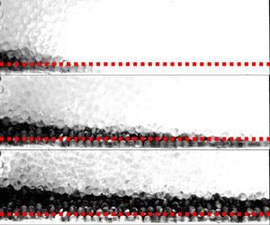
Figure 6. (a,b) Close-up snapshots of the gravity current thickness near the origin during two injection experiments with different flow rates. Photos are taken over 30 min (a) and 1 h (b), and spaced logarithmically in time. (a)  $Q = 0.209\,{\rm cm}^3\,{\rm s}^{-1}$, $H^* = 0.36$ cm; (b) $Q = 0.020\,{\rm cm}^3\,{\rm s}^{-1}$, $H^* = 0.11$ cm.
Data for the thickness and radius of the current are plotted together with numerical and analytical results in figure 5. The radius data  $R(t)$ approximately follow the $3/7$ power law (2.42), however, one could argue that the $1/2$ power law (2.17a,b) is just as accurate within the error margins of the experimental data. More clarity is achieved by observing the variation of the thickness near the origin $H(t)$, as shown by the photos in figure 6. In particular, the thickness is clearly observed to increase beyond the transition value by as much as $H\approx 5.5 H^*$ over the course of the experiments, albeit with a very small growth rate. Indeed, without running the experiments for such a long time it would appear that the thickness has ceased growing entirely. By contrast, when observed at logarithmically spaced time intervals the thickness shows no signs of abating. We estimate that the error associated with measuring the thickness of the current is approximately one bead diameter, so we have added error bars to illustrate this.
Post-processing of the images to extract the interface position reveals that the thickness follows the 1/7 power law (2.41) to good approximation, as shown in figure 5. We have also tried using a least-squares minimisation that fits an arbitrary power law  $H= A t^B$ to the combined experimental dataset (over four different flow rates) at late times $t>100 t^*$, as shown in the figure inset. This produces a power law of $B=0.1537\pm 0.0176$ which is close to $1/7\approx 0.1429$. Moreover, this slightly larger numerical value for the power law might hint towards the faster logarithmic growth predicted earlier.
It is not possible to discern the logarithmic correction to the thickness (2.44) quantitatively since this would require much longer time scales than we could achieve experimentally. Nor is it possible to accurately discern the convergence of the experimentally measured shape to the approximate solution (2.29) over long times, since the aspect ratio of the current is incredibly slender (around 200:1). To extend the experiments to larger values of  $t/t^*$ is challenging in practice, since smaller flow rates than $Q=0.02\,{\rm cm}^3\,{\rm s}^{-1}$ would result in current thicknesses much smaller than a single bead size ( $H^*\ll 0.3\,{\rm cm}$) that would be difficult to observe. Alternately one could run the experiments for a longer time, but this requires a much larger tank than we have available. For example to extend $t/t^*$ by a factor 100 would require a tank of dimensions $100^{3/7}\approx 7.2$ times larger (i.e. with a $439\,{\rm cm}\times 439\,{\rm cm}$ base). Nevertheless, our experiments clearly show an increasing thickness near the origin with the approximate 1/7 power law behaviour (2.41). Hence, by conservation of mass (2.24) it follows that the radius must grow according to a 3/7 power law, and the shape profile (2.29) must become a good approximation over long times (e.g. see analysis in § 2.4 and numerical solution in figures 2, 4).
It is important to note the possible effects of diffusion/dispersion over such long time scales. The length scales for molecular diffusion, fluid dispersion, and Taylor dispersion are approximately  $\ell \sim (D t)^{1/2}$, $\ell \sim (d U t)^{1/2}$ and $\ell \sim (d^2 U^2 t / 48D)^{1/2}$, respectively, where $D$ is the molecular diffusivity of salt or dye (both similar values), $U$ is a characteristic velocity scale and $d=0.3\,{\rm cm}$ is the diameter of the Ballotini beads. As an estimate for the diffusivity we take $D=10^{-10}\,{\rm m}^2\,{\rm s}^{-1}$, and for the velocity we take the value at the top of the current $U\approx \mathrm {d}H/\mathrm {d}t$. Inputting these, we calculate diffusion/dispersion scales of $\ell \sim 0.06\,{\rm cm}$, $\ell \sim 0.13\,{\rm cm}$ and $\ell \sim 0.04\,{\rm cm}$, which are all considered small within the experimental context. It is clear from the images in figure 6 that the interface near the origin remains relatively sharp (although there are some light scattering effects due to the glass beads), indicating that the effects of dispersion are negligible there. Hence, this validates our approach of post-processing the images to extract the current thickness at late times.
3. Relevance to carbon storage sites
In this section we situate our results within the context of carbon storage applications, in which CO $_2$ is injected into a porous reservoir saturated with brine and bounded above by an impermeable cap rock (note that, under the Boussinesq approximation, our analysis equally applies to a lighter fluid injected into a heavier fluid which is bounded above). The ability to determine whether an injected CO $_2$ plume is in a pressure-driven regime or a gravity-driven regime is useful for predicting the shape of the flow, and the expected plume migration speeds. This is important for ensuring that the CO $_2$ can be stored as safely and efficiently as possible.
For this analysis we compare our estimates for the transition time and thickness scalings  $t^*$, $H^*$, with typical parameter values from field sites. This enables us to estimate whether the required injection time, or whether the confines of the aquifer (e.g. the available space between impermeable cap rocks) are sufficient for a gravity current to form. To make this comparison we require approximate parameter ranges for the injection flux $Q$, as well as the buoyancy velocity $u_b=k_H\Delta \rho g/\mu$, porosity $\phi$ and anisotropy $\gamma =k_H/k_V$.
As described by Huppert & Pegler (Reference Huppert and Pegler2022) in the isotropic case, the time to transition to a gravity current may be significantly prolonged by small permeability values. Here, we show that the transition time (2.12) may be further prolonged by the presence of anisotropy, such that even sedimentary systems with large horizontal permeability values  $k_H$ may still remain in a pressure-driven regime for a long time (e.g. hundreds or thousands of years) if the vertical permeability $k_V$ is significantly smaller ( $\gamma \gg 1$). This has significant consequences for modelling approaches, which often directly assume a gravity-driven plume within the timeframe of the injection site, and indicates the need for detailed measurements of heterogeneities to ensure accurate predictions for the migration of CO $_2$.
$_2$.
In addition to the case of axisymmetric radial injection, which is the focus of the current study, we also briefly describe the analogous case of two-dimensional planar injection (from a line source) into anisotropic media. This is a simple extension of the study by Huppert & Pegler (Reference Huppert and Pegler2022) for isotropic media, incorporating different permeabilities  $k_H$, $k_V$, in the horizontal and vertical directions. As such, for the present analysis we skip the derivation of these scalings and simply present them in table 2 for reference. To distinguish the planar case from the radial (axisymmetric) case, we introduce subscript notation for the transition time $t^*_x$, the transition thickness $H^*_x$, and the injection flux per unit width $Q_x$. Likewise, the variables $R_x$ and $H_x$ in the planar case are equivalent to the lateral and vertical extents of the current. We note that the dynamics of the current for planar injection only depends on the anisotropy parameter $\gamma$ at early times, not at late times, as discussed in the Introduction. In figure 10 in Appendix B we have plotted additional data for the evolution of $R_x(t)$ and $H_x(t)$ in the planar case. These data include results from our numerical simulations (modified to a two-dimensional coordinate system) as well as some additional experiments that we conducted in a Hele-Shaw cell. Further details of these results are described in Appendix B.
Table 2. List of asymptotic limiting behaviours for the horizontal and vertical extent of the flow, as well as the transition scalings, for the case of planar injection (from a line source) and radial injection (from a point source). For example, the late-time extent in the radial case is given by  $R=\zeta _N(Q^2 u_b/\phi ^3)^{1/7}t^{3/7}\gamma ^{1/14}$. Note, the vertical extent in the case of radial injection $H$ has a slow logarithmic dependence (2.44) which we omit here for simplicity.

The references for the parameter values used in this section comprise a variety of sources describing different carbon storage sites around the world (Bickle et al. Reference Bickle, Chadwick, Huppert, Hallworth and Lyle2007; Chadwick, Noy & Holloway Reference Chadwick, Noy and Holloway2009; Oldenburg et al. Reference Oldenburg, Jordan, Nicot, Mazzoldi, Gupta and Bryant2011; Cowton et al. Reference Cowton, Neufeld, White, Bickle, White and Chadwick2016; Bickle et al. Reference Bickle, Kampman, Chapman, Ballentine, Dubacq, Galy, Sirikitputtisak, Warr, Wigley and Zhou2017; Jiang et al. Reference Jiang, Pekot, Jin, Peck, Gorecki and Worth2017; Williams & Chadwick Reference Williams and Chadwick2017; Cowton et al. Reference Cowton, Neufeld, White, Bickle, Williams, White and Chadwick2018; Roach & White Reference Roach and White2018). The buoyancy velocity is estimated using parameter values  $\mu = [5.5\unicode{x2013}6.6]\times 10^{-5}\,{\rm Pa}\,{\rm s}$, $\Delta \rho =232\unicode{x2013}309\,{\rm kg}\,{\rm m}^{-3}$ and $k_H=10^{-14}\unicode{x2013}10^{-12}\,{\rm m}^2$, resulting in $u_b=[3.4\unicode{x2013}551]\times 10^{-7}\,{\rm m}\,{\rm s}^{-1}$. For the injection flux, we take estimates for a two-dimensional line source as $Q_x=[0.4\unicode{x2013}3]\times 10^{-4}\,{\rm m}^2\,{\rm s}^{-1}$, and for a radial point source as $Q=[0.1\unicode{x2013}4]\times 10^{-2}\,{\rm m}^3\,{\rm s}^{-1}$. Porosity is taken as $\phi =0.2\unicode{x2013}0.25$. The degree of anisotropy varies considerably between CO $_2$ sequestration sites. For example, observations of permeability variations were around two orders of magnitude for Salt Creek, USA (Bickle et al. Reference Bickle, Kampman, Chapman, Ballentine, Dubacq, Galy, Sirikitputtisak, Warr, Wigley and Zhou2017), and four orders of magnitude for the Tilje formation in Norway (a potential sequestration site) (Martinius et al. Reference Martinius, Ringrose, Næss, Wen and Hentz1999; Bergmo et al. Reference Bergmo, Emmel, Anthonsen, Aagaard, Mortensen and Sundal2017). Hence, for this study we consider anisotropy in the range $\gamma =1\unicode{x2013}10^4$.
We note that in the case of sedimentary layers, the anisotropy parameter is interpreted as an effective property which is only well defined over length scales much larger than a single layer thickness (see § 2.1). Therefore, for the application of our model we restrict our attention to situations where the flow spans across a large number of layers or across a single sedimentary layer with significant anisotropy (i.e. due to compaction). In other situations (where the flow only occupies a few layers) a more detailed numerical model is required to treat the specific details of the flow within each layer.
Collating all of these data, we plot the transition time  $t^*$ and transition thickness $H^*$ in figure 7 for a range of anisotropy values, in both the planar and radial cases. Upper and lower bounds are displayed which correspond to the range of possible values for the injection flow rates $Q_x$, $Q$, buoyancy velocity $u_b$ and porosity $\phi$. The range of data displayed shows that transition may occur once the flow has reached depths of 10–1000 m at time scales of 1–10 years, for very anisotropic reservoirs. This indicates that some storage sites may actually be in a pressure-driven regime (rather than a gravity-driven regime) for a significant period of operation.

Figure 7. Transition time  $t^*$, $t_x^*$ (a) and transition thickness $H^*$, $H_x^*$ (b) for different anisotropy values $\gamma$, in the case of planar (line source) injection and radial (point source) injection. Corresponding data for the Aquistore carbon sequestration site (assuming radial injection) are illustrated, together with uncertainty estimates for parameter values.
For comparison, we also display data for the Aquistore CO $_2$ storage project in Saskatchewan, Canada (in operation 2015–present). In this case, the storage reservoir is at least 150 m thick and is located at a depth of 3200 m. This vertical interval is bounded above and below by low permeability layers of rock (see White et al. (Reference White, Roach, Roberts and Daley2014) for more details). The mean permeability within the storage reservoir is estimated as $k=1\times 10^{-14}\,{\rm m}^2$ (Roach & White Reference Roach and White2018). Likewise, Jiang et al. (Reference Jiang, Pekot, Jin, Peck, Gorecki and Worth2017) estimated the injection rate as 350–550 tonnes day $^{-1}$, which is equivalent to $Q\approx 5.3\unicode{x2013}9.2\times 10^{-3}\,{\rm m}^3\,{\rm s}^{-1}$. We model the injection as an axisymmetric point source. Hence, using approximate anisotropy values $\gamma =10\unicode{x2013}100$ we calculate a transition time scale of $t^*=40\unicode{x2013}1040$ days. The transition thickness is calculated as $H^*=98\unicode{x2013}163$ m, which is quite large due to the low permeability and high injection rates for this storage site. This indicates that the effects of the vertical confinement of the reservoir are likely to have played an important role on CO $_2$ migration before reaching this transition regime. Hence, the early-time dynamics (2.6)–(2.7) is appropriate for the early stages of injection for this site, after which a model which incorporates the effects of confinement may be more appropriate.
To analyse when and where the effects of confinement become important, one could use the results of Hesse et al. (Reference Hesse, Tchelepi, Cantwel and Orr2007) for the finite release of a buoyant fluid into a porous layer. For example, it was found that a similar regime transition is observed depending on how much of the vertical interval of the layer is occupied with the released fluid. Similarly, Pegler, Huppert & Neufeld (Reference Pegler, Huppert and Neufeld2014) investigated the effects of a viscosity contrast on the injection of CO $_2$ into a confined porous layer. In this case, it was found that confinement played a dominant role when the CO $_2$ occupied at least 10 % of the layer thickness.
4. Discussion
The transition from a pressure- to a gravity-driven flow has been addressed for constant axisymmetric injection into an anisotropic porous medium. We have derived scalings for the early and late-time growth of the current, as well as the time scale at which the transition occurs, showing close comparison with analogue experiments and numerical simulations. Early-time scalings revealed that anisotropy causes a long and thin current in which the pressure is not hydrostatic, with a delayed transition to the gravity-driven regime. Hence this study presents a paradigm shift for such flows, which are typically assumed to be gravity driven if long and thin. Analysis of the late-time regime showed that a region near the origin must remain pressure driven. Within this pressure-driven region, strong vertical velocities are required to deliver a uniform horizontal flow to the rest of the gravity-driven current. The pressure within this region cannot become hydrostatic, since this causes an unphysical singular current thickness near the origin. Therefore, the inner pressure-driven region serves to counteract this singularity, thereby providing a significant non-hydrostatic contribution to the flux even at late times.
One consequence of this pressure component is a finite but ever-growing thickness near the origin, which contrasts previous theories that assumed a constant thickness scaling. Another consequence is that the late-time growth of the gravity current remains affected by the vertical permeability value  $k_V$ (and hence the anisotropy ratio $\gamma$) due to vertical velocities near the origin. This is in contrast to the two-dimensional (planar) case, in which anisotropy only affects the time to transition, not the late-time behaviour. Our theoretical predictions were confirmed by comparison with numerical simulations of anisotropic Darcy flow run across 13 orders of magnitude in time, and porous medium tank experiments in the isotropic case. Length and time scales for transition were calculated for anisotropy values of different CO $_2$ storage sites, indicating that some field sites may never reach the gravity-driven regime over the course of operation.
It should be noted that in practice sequestration sites usually inject CO $_2$ over a finite length of perforations (at least metres, and sometimes tens of metres for long horizontal wells). Hence, it is worth discussing our assumption of a point source and how this compares with real injection scenarios. In particular, we expect our point source model to be less accurate in situations where the vertical extent of the plume is the same as or smaller than the injection interval (i.e. at the early stages of injection). However, once the plume has grown larger than this our model corresponds with the macroscopic flow behaviour, which does not depend on the specific details of the well geometry close to the source, only the injection rate. In a future study a more a detailed numerical model could be used to assess the effect of the precise well geometry at very early times.
Whilst we have mentioned carbon sequestration applications throughout this study, we have neglected several physical effects which are relevant to the flow of CO $_2$ in brine. For example, we have neglected the viscosity contrast between these phases for simplicity (CO $_{2}$ is typically around 20–30 times less viscous than brine). By extending this study to account for such effects, it is expected that the viscosity ratio $M=\mu _1/\mu _2$ will appear in the early and late dynamics for $H$ and $R$ wherever the anisotropy parameter $\gamma$ does. This is because the viscosity ratio can only affect the dynamics whenever the flow of injected and ambient fluids are coupled together (just like $\gamma$). It would also be interesting to extend these results to account for multiphase effects, similarly to Golding, Huppert & Neufeld (Reference Golding, Huppert and Neufeld2013) in the case of homogeneous media, and similarly to Benham, Bickle & Neufeld (Reference Benham, Bickle and Neufeld2021a) and Jackson & Krevor (Reference Jackson and Krevor2020) in the case of heterogeneous media.
There are several interesting perspectives from this work that are worth discussing. Firstly, the different dynamics between early and late times presents an opportunity for inverse modelling to help interpret petrophysical information about the reservoir. For example, if it can be shown that the radial extent of the flow is growing according to the early-time power law behaviour, then this can place bounds on the permeability and anisotropy of the flow due to heterogeneities. This is useful for field sites since information about the heterogeneities is often restricted to sparse core measurements or coarse seismic surveys.
It is also worth noting the analogy between the current study and the canonical case of a classical viscous gravity current. It is easy to follow the above analysis for the case of constant injection of a viscous fluid onto an impermeable substrate in either the planar or radial case. It transpires that similar scalings can be derived for the time and thickness required to transition from a pressure- to a gravity-driven flow. For example, in the radial case these are given by  $H^*=(Q\mu /\Delta \rho g)^{1/4}$ and $t^*=(2{\rm \pi} /3)(\mu ^3/(\Delta \rho g)^3 Q)^{1/4}$. However, it is not clear how the inner pressure-driven region affects the viscous gravity current at late times. In particular, the no-slip condition at the base of the current produces a different flow pattern to that considered here, making it difficult to translate our other results. Nevertheless, one could investigate such flow patterns by introducing tracers at the source of the gravity current, shedding light on the size and role of the pressure-driven region at late times.
Funding
This research is funded in part by the GeoCquest consortium, a BHP-supported collaborative project between Cambridge, Stanford and Melbourne Universities, and by a NERC consortium grant ‘Migration of CO $_2$ through North Sea Geological Carbon Storage Sites’ (grant no. NE/N016084/1).
Declaration of interests
The authors report no conflict of interest.
Appendix A. Further numerical details: boundary conditions and dimensionless equations
The full set of boundary conditions described in § 2.5 is given by
 $$\begin{gather} u=0:\quad \mathrm{at}\ r=r_0,\enspace z>z_0, \end{gather}$$
 $$\begin{gather}w=0:\quad \mathrm{at}\ z=0, \end{gather}$$
 $$\begin{gather}u = Q/(2{\rm \pi} r_0z_0):\quad \mathrm{at}\ r=r_0,\enspace z\leq z_0, \end{gather}$$
 $$\begin{gather}p={-}\rho_2 g z:\quad \mathrm{at}\ r=\ell, \end{gather}$$
 $$\begin{gather}p={-}\rho_2 g \ell:\quad \mathrm{at}\ z=\ell, \end{gather}$$
which correspond to impermeable/symmetric walls at  $r=r_0$ and $z=0$, imposing a constant input flux $Q$ over a small vertical interval of height $z_0$ near the origin and far-field hydrostatic pressure conditions imposed at the boundaries of a large but finite domain of size $\ell \times \ell$. In this formulation, $u$ is the cylindrical radial velocity and $w$ is the vertical velocity, which are each given by
 $$\begin{gather} u={-}\frac{k_H}{\mu}\frac{\partial p}{\partial r}, \end{gather}$$
 $$\begin{gather}w={-}\frac{k_V}{\mu}\left(\frac{\partial p}{\partial z}+ \rho_i g\right),\quad i=1,2, \end{gather}$$
where the subscript  $i=1,2$, inside/outside the injected flow region. By introducing dimensionless variables of the form
 \begin{equation} p={-}\rho_2 g z + \Delta\rho g \ell \hat{p},\quad z=\ell\hat{z},\quad r=\ell\hat{r},\quad u=u_b\hat{u},\quad w=u_b\hat{w}, \end{equation}
the governing equations and boundary conditions reduce to
 $$\begin{gather} \hat{\boldsymbol{\nabla}}\boldsymbol{\cdot} \hat{\boldsymbol{u}}=0:\quad \mathrm{on}\ \varOmega_1\cup\varOmega_2, \end{gather}$$
 $$\begin{gather}\hat{u}={-}\frac{\partial \hat{p}}{\partial \hat{r}}:\quad \mathrm{on}\ \varOmega_1\cup\varOmega_2, \end{gather}$$
 $$\begin{gather}\hat{w}={-}\frac{1}{\gamma}\left(\frac{\partial \hat{p}}{\partial \hat{z}} + 1\right):\quad \mathrm{on}\ \varOmega_1, \end{gather}$$
 $$\begin{gather}\hat{w}={-}\frac{1}{\gamma}\frac{\partial \hat{p}}{\partial \hat{z}}:\quad \mathrm{on}\ \varOmega_2, \end{gather}$$
 $$\begin{gather}\hat{u}=0:\quad \mathrm{at}\ \hat{r}=\hat{r}_0,\enspace \hat{z}>\hat{z}_0, \end{gather}$$
 $$\begin{gather}\hat{w}=0:\quad \mathrm{at}\ \hat{z}=0, \end{gather}$$
 $$\begin{gather}\hat{u} = \frac{\hat{Q}}{2{\rm \pi}}:\quad \mathrm{at}\ \hat{r}=\hat{r}_0,\enspace \hat{z}\leq \hat{z}_0, \end{gather}$$
 $$\begin{gather}\hat{p}=0:\quad \mathrm{at}\ \hat{r}=1, \end{gather}$$
 $$\begin{gather}\hat{p}=0:\quad \mathrm{at}\ \hat{z}=1, \end{gather}$$
where  $\hat {z}_0=z_0/\ell$, $\hat {r}_0=r_0/\ell$ and $\hat {Q}=Q/(r_0z_0u_b)$. Although we have written (A9)–(A17) in terms of both the pressure and the velocities (for convenience), the pressure is the only solution variable.
After introducing a dimensional time scale  $T=\ell \phi /u_b$, such that $t=T\hat {t}$, the equation for the motion of the fluid–fluid interface $\partial \varOmega =\boldsymbol {r}(t)$ (2.46), becomes
 \begin{equation} \frac{\mathrm{d}\hat{\boldsymbol{r}}}{\mathrm{d}\hat{t}}=\hat{\boldsymbol{u}} \left(\hat{\boldsymbol{r}},\hat{t}\right). \end{equation}
Likewise, the initial condition of the interface is given by
 \begin{equation} \hat{\boldsymbol{r}}(0)=\hat{\boldsymbol{r}}_0, \end{equation}
where we take  $\hat {\boldsymbol {r}}_0$ to be a very small hemisphere of radius $r_0$. Initial conditions for $\hat {p}$ are not needed since the pressure solution is determined by (A9)–(A17), given the interface position $\hat {\boldsymbol {r}}$. We note that since the flow is self-similar at early times (2.6)–(2.7), the solution quickly becomes independent of the precise initial conditions we impose (A19), provided they are sufficiently small.
We note that the dimensionless volume of fluid within region  $\varOmega _1$, which we denote $\hat {V}$, is given by
 \begin{equation} \hat{V}=\hat{Q}\hat{t}. \end{equation}
Hence, we see that by stretching time according to  $\hat {t}\rightarrow \hat {t}/\hat {Q}$, this is equivalent to replacing the inflow condition (A15) with
 \begin{equation} \hat{u} = \frac{1}{2{\rm \pi}}:\quad \mathrm{at}\ \hat{r}=\hat{r}_0,\enspace \hat{z}\leq \hat{z}_0. \end{equation}
In this way, we see that the only role of the parameter  $\hat {Q}$ is to stretch time, and consequently it can be removed from the problem without loss of generality. This indicates that the dimensionless problem only depends on one parameter, which is the anisotropy $\gamma$ (excluding the numerical parameters $\hat {z}_0$ and $\hat {r}_0$, since the solution does not depend on these provided they are sufficiently small).
Appendix B. Additional figures
In this section we present three additional figures together with brief descriptions of each. Firstly, figure 8 shows a comparison between the numerical solution described in § 2.5 (in the isotropic case  $\gamma =1$) and the classical similarity solution given by (2.17a,b). The discrepancy between the numerical and analytical predictions for the shape diverge for large times. This is because the numerical solution has a growing thickness $H(t)$, whereas the classical similarity solution predicts a constant thickness scaling. There is also a discrepancy in the growth of the radius, since the classical similarity solution predicts a faster power law growth of $R\sim t^{1/2}$ as opposed to $R\sim t^{3/7}$.

Figure 8. Numerical solution for the current shape  $z=h(r,t)$ (black dotted lines) in an isotropic medium $\gamma =1$, together with the self-similar solution (2.17a,b) (green lines). The vertical scale is stretched by $\times 10.5$ for illustration purposes.
Figure 9 shows exactly the same data as figure 5 except with a linear–linear (as opposed to log–log) scale. The axis ranges have been slightly reduced compared with figure 5 so that the experimental data can be seen more clearly.

Figure 9. Analytical, numerical and experimental data for the radial (a) and vertical (b) extents of the current,  $R$,
$R$,  $H$, plotted on a linear scale. These are exactly the same data as the log–log plots in figure 5.
Finally, figure 10 shows a comparison between numerical, analytical and experimental results for the evolution of the lateral and vertical extents of a two-dimensional (planar) gravity current in the case of a line source,  $R_x(t)$ and $H_x(t)$. Numerical results are achieved by following the same method as described in § 2.5 except using a two-dimensional coordinate system $x,z$. Analytical scalings for the evolution of the horizontal and vertical extent, $R_x(t)$ and $H_x(t)$, are summarised in table 2. For the experimental results, these consist of data taken from the porous bead experiments of Sahu & Neufeld (Reference Sahu and Neufeld2020) as well as our own data taken from experiments in a Hele-Shaw cell with glycerol injected into air. These are summarised below.

Figure 10. Analytical, numerical and experimental data for the radial (a) and vertical (b) extents of a two-dimensional current,  $R_x$, $H_x$. Numerical results are shown for both an isotropic medium $\gamma =1$ and an anisotropic medium $\gamma =10^4$, whereas experimental results are only for the isotropic case. Analytical early- and late-time scalings (see table 2), are shown with solid black lines.
In our Hele-Shaw experiments, a constant flow rate of glycerol dyed with red food colouring is injected (via a peristaltic pump) into the narrow gap between two Perspex plates above an impermeable substrate. The plates are aligned vertically so that gravity acts in the same plane as the gap, and a video camera captures the evolution of the flow at 24 frames per second. Different flow rates and gap widths are explored by varying the pump speed and the gap spacing accordingly. The flow rate  $Q$ is calculated using a mass balance over time. The porosity is taken as $\phi =1$ and the effective permeability of the medium is given by $k=\delta ^2/12$, where $\delta$ is the gap width. Since it is difficult to estimate $\delta$ very accurately (e.g. within fractions of a millimetre), this is instead calculated using a parameter fitting step. Specifically, we integrate the observed cell area occupied by the injected fluid ( $\mathcal {A}$) and compare this with the volume change measured by the mass balance, such that $\mathcal {A}\delta =Qt$, finding the value of $\delta$ which fits this best. The density difference between the two fluids is measured as $\Delta \rho =1229\unicode{x2013}1.225\,{\rm kg}\,{\rm m}^{-3}$ and the viscosity of the glycerol is taken as $\mu =0.765\,{\rm Pa}\,{\rm s}$. For glycerol injected into air the effects of surface tension are considered small (Huppert & Woods Reference Huppert and Woods1995).
By varying the input flow rate and gap width, different transition time scales  $t_x^*$ are achieved, allowing observation of early-, intermediate- and late-time behaviours. The full data range spans $t/t_x^*=0.02\unicode{x2013}24$, and we complement this with the experimental data of Sahu & Neufeld (Reference Sahu and Neufeld2020), which extend up to a value of $t/t_x^*=8341$. The latter experiments investigated dispersive effects in a tank filled with porous beads rather than in a Hele-Shaw cell, and the fluid pairing was salty and fresh water rather than glycerol and air. Nevertheless, the data can be compared directly, by re-scaling time and space according to $t_x^*,H_x^*$.
All the experimental data are plotted in figure 10, showing good comparison with the numerical calculations and the analytical scalings at early and late times. Hence, this further reinforces confidence in our numerical scheme and demonstrates the validity of our analytical approach for deriving the different regime scalings.


 Open access