





1. Introduction
Worldwide efforts are carried out to reduce our dependence on fossil fuels due to their harmful effects on the environment and their non-renewable character. Wind power is one of the most attractive alternatives of renewable and clean source of energy due to its potential and availability. The growth of wind energy worldwide has been continuous in the last decades leading to the increase of the number of wind turbines onshore and offshore. The clustering of wind turbines facilitates the project considerably since the cost per turbine decreases. Optimisation algorithms are often used to decrease electrical losses or visual and social impact. While onshore wind farms follow a layout driven by the terrain to exploit the eventual speedups, offshore farms are limited by the feasible locations where the sea depth is neither too shallow nor too deep, enabling the construction of the foundation and the installation of the turbines. Similar to other renewable energy sources, wind energy is characterised by a low power density, namely the ratio between the produced power and the area occupied by the turbines. On average a wind farm with regular layout produces a power of  $5\text {--}10\ \textrm {W}\ \textrm {m}^{-2}$ of land area and this number does not depend on the diameter of the turbines (MacKay Reference MacKay2008).
Power production measurements over real farms indicate that the first row of turbines facing the wind is the most producing (only wind farms over flat terrain or offshore will be considered in the present discussion), while the other turbines produce less due to wake losses. If the layout is regular (as for instance is the case of equispaced turbines), the power production has an approximate plateau, suggesting that a nearly parallel state is achieved in the velocity statistics somewhere downwind of the farm leading edge. This is true for the infinite-farm case (Calaf, Meneveau & Meyers Reference Calaf, Meneveau and Meyers2010), but it is approximately true also for finite-length configurations (Chamorro, Arndt & Sotiropoulos Reference Chamorro, Arndt and Sotiropoulos2011; Bossuyt, Meneveau & Meyers Reference Bossuyt, Meneveau and Meyers2018). However, a paradox emerges from the parallel argument: if the flow is nearly parallel, the horizontal flux of energy upwind and downwind of every wind turbine (sufficiently downwind of the first rows) must be equal but the turbine in-between is anyhow extracting power from the flow. The only flux of energy able to sustain the power extraction in a parallel case (without introducing an artificial pressure gradient) is the energy flux from above the turbines. Moreover, since the turbines are applying a drag force to the flow, the absorbed momentum must be balanced by a decrease of the pressure through the farm (as for instance in the infinite farm case) or by the growth of an internal boundary layer on top of the farm.
With the growth of wind energy there has been interest in developing modelling tools to predict wind-turbine performance in a large wind farm, where the wakes created by upwind wind-turbines can significantly reduce the power production of downwind ones and therefore the performance of the whole farm. There are already a significant number of studies that have focused on the structure of wakes from individual wind turbines (Medici & Alfredsson Reference Medici and Alfredsson2006; Segalini & Alfredsson Reference Segalini and Alfredsson2013; Bastankhah & Porté-Agel Reference Bastankhah and Porté-Agel2014). Several empirical wake models have been proposed in the wind-energy community based on experimental, numerical and theoretical arguments (Katic, Højstrup & Jensen Reference Katic, Højstrup and Jensen1987; Ainslie Reference Ainslie1988; Braunbehrens & Segalini Reference Braunbehrens and Segalini2019). However, the wake models provide uncertainty especially for what concerns the wake interaction, often assumed to be best replicated by the sum of the squares of the velocity deficits, according to the current best practice. These models can be considered ‘bottom-up’ approaches to the problem of understanding the structure of large wind farms.
Previous studies comprise a large amount of experimental (Cal et al. Reference Cal, Lebrón, Castillo, Kang and Meneveau2010; Chamorro & Porté-Agel Reference Chamorro and Porté-Agel2010, Reference Chamorro and Porté-Agel2011; Iungo Reference Iungo2016) and numerical (Wu & Porté-Agel Reference Wu and Porté-Agel2011; Meyers & Meneveau Reference Meyers and Meneveau2012; Yang, Kang & Sotiropoulos Reference Yang, Kang and Sotiropoulos2012; Wu & Porté-Agel Reference Wu and Porté-Agel2013) approaches to better understand the interaction of turbulent flow with a distributed array of wind turbines. Large-eddy simulation results (Stevens, Gayme & Meneveau Reference Stevens, Gayme and Meneveau2014, Reference Stevens, Gayme and Meneveau2016) and wind-tunnel measurements (Chamorro & Porté-Agel Reference Chamorro and Porté-Agel2011; Bossuyt et al. Reference Bossuyt, Howland, Meneveau and Meyers2017, Reference Bossuyt, Meneveau and Meyers2018) show that after approximately 10 rows, the average row power becomes independent of the row number, thus indicating the approach of a fully developed regime. Abkar & Porté-Agel (Reference Abkar and Porté-Agel2014) examined the mean and turbulent kinetic energy budgets of very large wind farms in a conventionally neutral boundary layer. The works of Cortina, Calaf & Cal (Reference Cortina, Calaf and Cal2016) and Allaerts & Meyers (Reference Allaerts and Meyers2017) have demonstrated that there exists two mean kinetic energy (MKE)-based mechanisms that primarily contribute to the wake's recovery. These are the advection and the vertical flux of MKE. Results from Cortina, Sharma & Calaf (Reference Cortina, Sharma and Calaf2017) in a very large wind farm indicated that these mechanisms are modulated by the background thermal stratification, as well as the wind farm density. For low density wind farms advection dominated the wake recovery, while for high density wind farms the MKE recovered through turbulent fluxes. For the cases in-between, a smooth balance of both mechanisms existed. Significant numerical work has been devoted to the effect of atmospheric stratification and Coriolis force (Allaerts & Meyers Reference Allaerts and Meyers2017; Wu & Porté-Agel Reference Wu and Porté-Agel2017) on the farm aerodynamics, although these aspects will not be investigated in the present work.
To help understanding basic trends and overall asymptotic limits, it is important to have simple physics-based models with relatively few terms. Following this aim, the problem was approached from another (‘top-down’) direction where the wind turbines in a large array are modelled as surface roughness elements, leading to an increased roughness length that needs to be parameterised. This idea was introduced by Newman (Reference Newman1977) and Lissaman (Reference Lissaman1979) and further developed by Frandsen (Reference Frandsen1992) and Frandsen et al. (Reference Frandsen, Barthelmie, Pryor, Rathmann, Larsen, Høstrup and Thøgersen2006) who proposed a one-dimensional, single-column-type model that replaced the complex three-dimensional structure of a wind farm with a horizontal average often used to describe turbulent flows in canopies (Raupach & Shaw Reference Raupach and Shaw1982; Raupach, Coppin & Legg Reference Raupach, Coppin and Legg1986; Raupach, Finnigan & Brunet Reference Raupach, Finnigan, Brunet, Garratt and Taylor1996; Yang et al. Reference Yang, Raupach, Shaw, Paw U and Morse2006; Segalini, Fransson & Alfredsson Reference Segalini, Fransson and Alfredsson2013). This was formulated as an equation for the mean horizontal velocity based on a vertical integration of the momentum equation. In the Frandsen top-down model, it was assumed that there is a constant momentum flux above the wind farm with a characteristic friction velocity,  $u_{*{hi}}$, while another constant stress region occurs below the hub height, $z_h$, with characteristic friction velocity, $u_{*{lo}}$. The difference between the two momentum fluxes (above and below the turbines) is given by the momentum loss caused by the turbines, assumed to be concentrated at hub height. This approach was used to deduce an effective roughness length $z_{0,{hi}}$ that describes the entire wind farm by means of a roughness analogy.
By means of an integral analysis of the kinetic energy balance, the kinetic energy fluxes associated with the Reynolds shear stresses was found to be of the same order of magnitude as the power extracted by the wind turbines, highlighting the importance of the vertical fluxes of kinetic energy and the interaction of the wind farm with the atmospheric boundary layer (ABL) (Cal et al. Reference Cal, Lebrón, Castillo, Kang and Meneveau2010; Calaf et al. Reference Calaf, Meneveau and Meyers2010; Hamilton et al. Reference Hamilton, Kang, Meneveau and Cal2012; VerHulst & Meneveau Reference VerHulst and Meneveau2014). The model was used to provide insights into the optimal spacing between wind turbines in large wind farms (Meyers & Meneveau Reference Meyers and Meneveau2012; Stevens et al. Reference Stevens, Gayme and Meneveau2016). In particular, Meneveau (Reference Meneveau2012) proposed a new top-down model that combined the Frandsen approach with a model of the growth of internal boundary layers to include entrance effects. Later, a coupled wake-boundary layer model was presented by Stevens, Gayme & Meneveau (Reference Stevens, Gayme and Meneveau2015) describing the distribution of the power output in a wind-farm. The model coupled the wake expansion/superposition approach with a top-down model for the overall wind-farm boundary-layer structure. The wake expansion/superposition model captured the effect of turbine positioning, while the top-down portion added the interaction between the wind-turbine wakes and the ABL.
The oscillatory motion of the turbines wake is another crucial factor in wind farms because it increases the fatigue loads on the turbines. As already found in previous works (Medici & Alfredsson Reference Medici and Alfredsson2006; España et al. Reference España, Aubrun, Loyer and Devinant2012; Coudou, Buckingham & van Beeck Reference Coudou, Buckingham and van Beeck2017; Stevens & Meneveau Reference Stevens and Meneveau2017; Braunbehrens & Segalini Reference Braunbehrens and Segalini2019), the dominant dynamical phenomenon present in long wind farms is the meandering of the turbine wakes. Two main possible reasons for the formation of wake meandering have been suggested over the past few years: intrinsic instabilities of the wake associated with a periodic vortex shedding within the wake (Medici & Alfredsson Reference Medici and Alfredsson2006; España et al. Reference España, Aubrun, Loyer and Devinant2012), or the effect of the large-scale turbulent eddies contained in the ABL as observed for plume-dispersion analysis (España et al. Reference España, Aubrun, Loyer and Devinant2012). España et al. (Reference España, Aubrun, Loyer and Devinant2012) assumed that small-scale eddies (i.e. smaller than the rotor diameter), constituting the high-frequency part of the turbulence spectrum, are responsible for diffusive effects in the wake only, whereas the low-frequency part, composed of eddies larger than the rotor diameter, acts to transport the wake as a whole. Later, Coudou et al. (Reference Coudou, Buckingham and van Beeck2017) found that the formation of wake meandering seems to be neither entirely due to the intrinsic instabilities of the wake associated with a periodic vortex shedding, nor just due to large-scale turbulent eddies contained in the ABL. Rather, the wake-meandering formation appeared to be due to a combination of both of these mechanisms. So, the formation of wake meandering appears to be caused by the amplification of the intrinsic instabilities of the wake by large-scale turbulent eddies within the ABL.
The present work focuses on describing the horizontally averaged structure of the flow above a farm and on the interaction of the ABL with the wind-turbine array. The latter is expected to be characterised by the internal boundary layer in order to understand how the energy is transferred from the free stream (which contains a significant amount of energy) to the wind farm. The present paper is structured as follows. In § 2 an integral analysis of the governing equation (averaged in time and space) above the wind farm is proposed in order to identify new relations between the vertical energy flux of kinetic energy and the growth of the internal boundary layer. Section 3 describes the set-up used during the experimental campaign. In § 4 some relations for the turbulent shear stress and for the vertical flux of the MKE are proposed, highlighting the dominant terms of the integrated governing equation from the experimental results. Also shown is a comparison between the different layouts in terms of vertical flux. Furthermore, a self-similar analysis is proposed to identify the self-similarity of the velocity statistics above the farm including an attempt to describe the statistics by means of the diagnostic plot (Alfredsson, Segalini & Örlü Reference Alfredsson, Segalini and Örlü2011). The section reports finally a spectral analysis to describe how the energy is distributed amongst the various frequencies demonstrating the emergence and dominance of a large-scale peak, most likely related to the wake-meandering phenomenon. The section includes also some considerations about the spectra of the various velocity components and how do they agree when normalised with the integral time scale. Section 5 summarises the findings made in the present work with some concluding remarks.
2. Integral analysis of the governing equations
As anticipated in the introduction, the characterisation of the flow of kinetic energy above the wind farm is the main focus of the present work. This task is facilitated by the vertical integration of the flow equations in terms of momentum and kinetic energy, providing a framework to analyse the experimental results. The continuity, Navier–Stokes and energy equations are averaged in time and space by means of the standard time-average operator and of a spatial horizontal filter, respectively. The latter is introduced as
 \begin{equation} \langle \phi\rangle=\frac 1{S_xS_y}\int_{S_x\times S_y}\phi\,\mathrm{d}\kern0.7pt x\,\mathrm{d}y, \end{equation}
where the horizontal filter size has dimension  $S_x$ and $S_y$ in the streamwise ( $x$) and lateral ( $y$) directions, respectively, while $z$ will indicate the wall-normal (or vertical) direction in the following. The use of the filter allows us to approximately obtain a two-dimensional mean velocity field, thus helping to understand the macroscopic structure of the momentum transport in the vertical direction. The two filters applied sequentially (in time and space) imply the presence of fluctuations in time and space, so that any quantity is here decomposed as $\phi =\varPhi +\phi '$ with $\varPhi =\bar {\phi }$ indicating the time average (upper case variables will indicate time-averaged quantities to facilitate the notation) and $\phi '$ indicating the time-wise fluctuation. Analogously, the spatially filtered quantities will be decomposed as $\phi =\langle \phi \rangle +\phi ''$, where the first term is the spatial average and the second term is the spatial fluctuation (so that the relationships $\langle \langle \phi \rangle \rangle =\langle \phi \rangle$ and $\langle \phi ''\rangle =0$ approximately hold depending on the filter size). The time average of the product $ab$ will be $\overline {ab}=AB+\overline {a'b'}$ while the subsequent use of the spatial-average operator will lead to $\langle \overline {ab}\rangle =\langle A\rangle \langle B\rangle + \langle A''B''\rangle + \langle \overline {a'b'}\rangle$. The term $\langle \overline {a'b'}\rangle$ is the Reynolds stresses spatially averaged while $\langle A''B''\rangle$ is the dispersive stress: the latter represents the spatial fluctuations of the mean velocity field and emerges from the nonlinear term averaged in space and time.
The instantaneous velocity field in the streamwise, spanwise and vertical direction will be indicated by  $u=u_1$, $v=u_2$ and $w=u_3$, respectively. The pressure will be indicated by $p$, while the density and kinematic viscosity are denoted as $\rho$ and $\nu$, respectively. The application of the time- and space-average operators to the continuity equation leads to
 \begin{equation} \frac{\partial\langle U_i \rangle}{\partial x_i} = 0. \end{equation}
The time- and space-averaged steady Navier–Stokes equation becomes
 \begin{equation} \langle U_j\rangle \frac{\partial\langle U_i\rangle}{\partial x_j} ={-}\frac 1\rho\frac{\partial\langle P \rangle}{\partial x_i} + \nu\frac{\partial^{2}\langle U_i\rangle}{\partial x_j^{2}} - \frac{\partial r_{ij}}{\partial x_j}, \end{equation}
where  $r_{ij} = \langle \overline {u_i'u_j'}\rangle + \langle U_i''U_j'' \rangle$ indicates the summation of the Reynolds and dispersive stresses. In the following equations the viscous transport term will be neglected when involving averaged quantities because it is expected to be small away from solid surfaces, as in the present case. The averaged pressure term $\langle P \rangle$ was not measured during the experiment; however, since the vertical velocity is expected to be small, the vertical momentum conservation equation leads to
 \begin{equation} \frac{\partial}{\partial z}\left(\frac 1\rho\langle P \rangle+r_{33}\right) \approx 0\,\longrightarrow\, \frac 1\rho\langle P\rangle(x,\,z)\approx{-}\frac{U_e(x)^{2}}{2}-k_{e}(x)-r_{33}(x,\,z), \end{equation}
where  $U_e(x)$ indicates the velocity outside of the internal boundary layer. In (2.4) the term $k_e(x)=(r_{11e}+r_{22e}-r_{33e})/2$ denotes the difference between the free stream turbulent kinetic energy, if present, and $r_{33e}=\overline {w'^{2}}(z\to \infty )$. By means of (2.4) it is possible to rewrite the streamwise momentum equation as
 \begin{equation} \frac{\partial\langle U\rangle^{2}}{\partial x} + \frac{\partial\langle U\rangle\langle W\rangle}{\partial z} = U_e\frac{\mathrm{d}U_e }{\mathrm{d}\kern0.7pt x}+\frac{\mathrm{d}k_e }{\mathrm{d}\kern0.7pt x} - \frac{\partial\, \left(r_{11}-r_{33}\right)}{\partial x} - \frac{\partial r_{13}}{\partial z}. \end{equation}
The term  $r_{12}$ is not present in the (2.5) for symmetry reasons.
The mechanical energy conservation equation for the averaged flow can be obtained by multiplying (2.3) by  $\langle U_i\rangle$, obtaining at leading order,
 \begin{equation} \frac{\partial}{\partial x_j}\left[ \frac 12\langle U_j\rangle\langle U_i\rangle^{2} +r_{ij}\langle U_i\rangle + \frac 1\rho \langle P\rangle\langle U_j\rangle \right] = r_{ij}\frac{\partial\langle U_i\rangle}{\partial x_j}. \end{equation}
The last term of (2.6) represents the term transferring energy from the mean flow to the fluctuating flow in time and space.
2.1. Derivation of the von Kármán equation and of the integrated energy equation
The von Kármán equation, valid above the wind farm, can be obtained by integrating equation (2.5) between  $z_{0}$ and $z_{f}$ in the vertical direction, where $z_{0}$ is the closest position measured above the wind farm, while $z_{f}$ is the farthest. This leads to
 $$\begin{gather} -r_{13}(z_0) = \frac{\mathrm{d}}{\mathrm{d}\kern0.7pt x}\left( U_e^{2}\theta \right) + \delta^{*}U_e\frac{\mathrm{d}U_e }{\mathrm{d}\kern0.7pt x} - W_0\left( U_e - U_0 \right) \nonumber\\ - \frac{\partial}{\partial x}\int_{z_0}^{z_f}\left(r_{11}-r_{33}\right)\,\mathrm{d}z + \frac{\mathrm{d}}{\mathrm{d}\kern0.7pt x}\int_{z_0}^{z_f}k_e\,\mathrm{d}z , \end{gather}$$
where  $\delta ^{*}$ and $\theta$ are the displacement and momentum thickness defined, respectively, as
 \begin{equation} \delta^{*} = \int_{z_0}^{z_f}\left( 1 - \frac{\langle U\rangle}{U_e} \right) \,\mathrm{d}z,\quad \theta = \int_{z_0}^{z_f}\frac{\langle U\rangle}{U_e}\left( 1 - \frac{\langle U\rangle}{U_e} \right)\,\mathrm{d}z, \end{equation}
while  $U_0=\langle U\rangle (z_0)$ and $W_0=\langle W\rangle (z_0)$. It is worth pointing out that the integration starts from the top farm here, $z_0$, so that the bottom velocities are not zero. The shear stresses $r_{13}(z_f)\approx 0$ because the free stream turbulence is assumed to be isotropic.
The integrated energy equation for the averaged flow was obtained by integrating equation (2.6) as
 \begin{equation} \frac{\partial}{\partial x}\int_{z_0}^{z_f}T_x\,\mathrm{d}z + \left[ T_z \right]^{z_f}_{z_0} = \int_{z_0}^{z_f}D\,\mathrm{d}z , \end{equation}
where
 \begin{gather} T_x = \frac 12\langle U\rangle\langle U_i\rangle^{2} +\langle U\rangle\left(r_{11}-r_{33} \right)+ \langle{W}\rangle r_{13} - \langle U \rangle\frac{U_e^{2}}{2}-\langle U\rangle k_e, \end{gather}
 \begin{gather} T_z = \frac 12\langle W\rangle\langle U_i\rangle^{2} + \langle{U}\rangle r_{13}-\langle W\rangle \frac{U_e^{2}}{2} -\langle W\rangle k_e, \end{gather}
 \begin{gather} D = r_{11}\frac{\partial\langle U\rangle}{\partial x} + r_{13}\left(\frac{\partial\langle W\rangle}{\partial x}+\frac{\partial\langle U\rangle}{\partial z}\right) + r_{33}\frac{\partial\langle W\rangle}{\partial z}. \end{gather}
 The dominant terms of (2.9) can be obtained through an analysis of their orders of magnitude. It is expected that  $W\ll U$, $r_{11} \approx r_{33} \ll U^{2}$ and that $W(z_f),\,r_{13}(z_f) \approx 0$. The leading contribution to the kinetic energy will indeed come from $\langle U\rangle ^{2}/2$. By means of this leading-term analysis, one obtains a simplified energy equation as
 \begin{align} &\frac 12\frac{\partial}{\partial x}\int_{z_0}^{z_f}\langle U\rangle^{3}\,\mathrm{d}z -\frac 12\frac{\partial}{\partial x}\left[U_e^{2}\int_{z_0}^{z_f}\langle{U}\rangle \,\mathrm{d}z\right] - U_0 r_{13}(z_0)\nonumber\\ &\quad + \frac 12 W_0\left( U_e^{2} - U_0^{2} \right) = \int_{z_0}^{z_f}r_{13}\frac{\partial\langle U\rangle}{\partial z}\,\mathrm{d}z, \end{align}
where  $\langle U\rangle r_{13}$ is the turbulence-induced vertical flux of MKE. By introducing the energy thickness $\delta _e$ (Buresti Reference Buresti2012), (2.13) can be rewritten as
 \begin{equation} - U_0 r_{13}(z_0) + \frac 12 W_0\left( U_e^{2} - U_0^{2} \right) = \frac{\mathrm{d}}{\mathrm{d}\kern0.7pt x}\left(\delta_e U_e^{3}\right) + \int_{z_0}^{z_f}r_{13}\frac{\partial\langle U\rangle}{\partial z}\,\mathrm{d}z, \end{equation}
with  $\delta _e$ defined as
 \begin{equation} \delta_e = \frac 12\int_{z_0}^{z_f}\frac{\langle U \rangle}{U_e}\left( 1-\frac{\langle U \rangle^{2}}{U_e^{2}} \right)\, \mathrm{d}z. \end{equation}
 Equation (2.14) includes the vertical velocity  $W_0$ that is hard to measure above the farm. To circumvent this problem, $W_0$ is obtained from the von Kármán equation, so that (2.14) is approximated by
 \begin{equation} r_{13}(z_0)\frac{\left(U_e - U_0 \right)}2 +\frac{\mathrm{d}\left( U_e^{2}\theta\right)}{\mathrm{d}\kern0.7pt x}\frac{\left(U_e+U_0\right)}2 = \frac{\mathrm{d}}{\mathrm{d}\kern0.7pt x}\left(\delta_e U_e^{3}\right) + \int_{z_0}^{z_f}r_{13}\frac{\partial\langle U\rangle}{\partial z}\,\mathrm{d}z. \end{equation}
3. Experimental set-up
The experiments were performed in the minimum turbulence level (known as MTL) wind tunnel at KTH. The facility is a closed loop wind tunnel with a test section 7 m long, 1.2 m wide and 0.8 m high. The test section height was maintained constant throughout the experiments to have a simple and well-determined boundary condition during the measurement campaign. Before the test section a series of honeycombs and meshes were present followed by a contraction with an area ratio of  $9:1$. The tunnel has a heat exchanger to maintain the operating temperature constant within ${\pm }0.01\,^{\circ }\textrm {C}$.
The test section floor was covered with 4 m long steel plates to place the wind turbines. These were positioned by means of magnets placed at the bottom of the tower, giving high freedom in the layout choice. At the inlet of the test section a Prandtl tube was installed to monitor the wind-tunnel speed and to calibrate the hot-wire anemometer. The velocity inlet was kept fixed at  $U_{inlet} \approx 8\ \textrm {m}\ \textrm {s}^{-1}$ throughout the experimental campaign and it was used to normalise all of the velocity data. The dynamic pressure of the Prandtl tube was measured with a Furness FCO510 micromanometer with an uncertainty of 0.25 %. Two Pt100 probes were installed to monitor and control the tunnel temperature.
Two X-type hot-wire anemometers were used to characterise the velocity field. These were traversed in the domain by means of a three-axis traversing controlled by the measurement computer. The two probes had a fixed spanwise relative distance of  $D=45\ \mathrm {mm}$, corresponding to the diameter of the used wind-turbine model, and were placed at the same vertical height and streamwise position. An S-shaped probe support was manufactured to reduce the blockage effect of the traversing on the measuring probes. One X-wire measured the streamwise and vertical velocity components, while the other measured the streamwise and spanwise components, providing a nearly complete characterisation of the Reynolds stress tensor. Both probes were placed in the middle of the test section and were traversed in a volume starting from the turbine top ( $z=z_0$) up to approximately $7D$, length longer than the farm streamwise extension and depth equal to $3D$, i.e. the lateral spacing between two turbines in the considered farms: by assuming a spanwise periodic flow with negligible side effects, this should ensure the full characterisation of the flow evolution and enable the spatial averaging. After the farm trailing edge, the region below the turbine top was also characterised for an additional $15D$ since no turbines were present there. A Dantec streamline system was used in constant-temperature mode for all the four wires. The velocity at each measurement point was acquired for 20 s with a sampling frequency of 20 kHz. The characterisation of each farm configuration took two to three days including the measurement time, traversing time and calibration time performed automatically every 12 h to avoid drift in the hot-wire measurements. The ambient temperature inside the test section was also measured independently from the heat exchanger thermometer to apply (eventual) temperature-drift corrections to the hot-wire reading.
The calibration of the probes was done in two steps. First, a directional calibration was performed for both probes to characterise the angular coefficient of the probe,  $\gamma$, according to the sum and difference method (Bruun Reference Bruun1995; Segalini et al. Reference Segalini, Fransson and Alfredsson2013). Once the coefficient was determined, the probes were mounted in their measurement support and calibrated only in velocity, providing the calibration relationship between voltage and effective velocity for the $i\mathrm {th}$ probe, $U_{e,i}=F(E_i)$. From the two obtained effective velocities (measured with a single X-wire), the instantaneous flow velocities were calculated as
 \begin{equation} U=\dfrac{1}{2}\left(U_{e1}+U_{e2}\right)\quad\mathrm{and}\quad V=\frac{\gamma}{2}\left(U_{e1}-U_{e2}\right). \end{equation}
 No spires were used at the inlet of the test section so that the natural boundary layer present at the test-section floor was present. In order to investigate the effect of free stream turbulence, two different grids with square mesh size  $M/D=0.56$ and $M/D=1.12$ were used. Figure 1 shows the inlet profile of the streamwise velocity and of the velocity variances with and without the upstream grid. The edge of the incoming boundary layer was in any case below the bottom tip of the turbine models located at $z/D\approx 1$ (with $z=0$ indicating the ground). The boundary layer without grids was turbulent near the wall, but the turbulent fluctuations became negligible above where the flow velocity was nearly constant in the vertical direction. With the grid, the boundary layer became thicker as similarly did the region characterised by significant velocity fluctuations. Outside the edge of the near-wall region, the velocity fluctuations had the same magnitude in all components, as typical in isotropic grid turbulence. The integral time scale is also reported for the case with and without grids: despite the different mesh size, the time scale of the turbulent structures is comparable, so that the grids provide additional turbulent structures with similar dynamics, although the thickness of the boundary layer is higher for $M/D=0.56$.
Inlet profiles (measured at  $x/D=-10$) of ( $a$) streamwise velocity $U$, ( $b$) standard deviation $\sigma _u$, ( $c$)
$c$)  $\sigma _v$, ( $d$)
$d$)  $\sigma _w$, ( $e$) integral time scale, $\varLambda _u$, for the clean inflow (black lines), for the grid with $M/D=1.1$ (red lines) and for the grid with $M/D=0.56$ (blue lines).

3.1. Turbine details
Up to 152 turbines were involved in the present measurement campaign. These were freely rotating two-blade plastic rotors with diameter  $D=45\ \mathrm {mm}$, similar to what was already used by Ebenhoch et al. (Reference Ebenhoch, Muro, Dahlberg, Hägglund and Segalini2017) and Segalini & Dahlberg (Reference Segalini and Dahlberg2020). The hub (located at $z_{hub}=60\ \mathrm {mm}=1.33D$ from the ground) consisted of a tube of $3\ \mathrm {mm}$ diameter with friction bearings holding the rotor, while a tower with the same diameter was used to support nacelle and rotor. A magnetic foot of diameter 10 mm and height 3 mm was glued to the tower: the magnet was sufficiently strong to avoid the displacement of the turbine subjected to the approaching wind.
A strain gauge balance was used to characterise the small thrust force of the rotor. The thrust coefficient was found to be  $C_T=2T/(\rho U_{inlet}^{2}A_d)\approx 0.59+0.002U_{inlet}$ ( $A_d={\rm \pi} R^{2}={\rm \pi} D^{2}/4$ indicates the rotor area) with a weak dependence from the velocity magnitude. Furthermore, the turbines rotate with a tip-speed ratio $\lambda =\varOmega R/U_{inlet}\approx 4.8$, thereby quite fast due to their small size.
The wake downwind of a rotor was characterised at five different planes behind four aligned wind turbines in a separate experiment and the results were averaged to obtain an ensemble of the wake velocity deficit (the distance between the turbines was 20 $D$, sufficient enough to limit upstream wake effects but providing some weak turbulence before each turbine). Figure 2 shows the mean velocity field in the axial and in-plane directions and the standard deviation of the axial component. It is quite remarkable that the tower leaves a significant footprint downwind of the turbine, despite its small size compared with the rotor (the frontal area ratio between the tower and the rotor is just 11 %), but it has a profound effect in both the mean velocity and the standard deviation, with a intensity comparable with the tip vortices at the closest plane. However, already at 3 $D$ downwind of the rotor the wake of the tower becomes less intense and it vanishes. The wake deficit tends to move downward merging with the deficit of the tower, as indicated by the circles in figure 2 which mark the wake centre. The angular velocity behind the rotor is relevant only within the rotor area (Segalini & Alfredsson Reference Segalini and Alfredsson2013) and vanishes within the first 6 $D$ from the rotor.
Mean streamwise velocity (a–e), in-plane velocity (f–j) and streamwise velocity standard deviation (k–o). All velocities are scaled by the tunnel inlet velocity for ( $a{,}f{,}k$) $x/D=1.2$, ( $b{,}g{,}l$) $x/D=3.4$, ( $c{,}h{,}m$) $x/D=5.6$, ( $d{,}i{,}n$) $x/D=7.8$ and ( $e{,}f{,}o$) $x/D=10.0$. The circles in panels (a–e) indicate the minimum velocity deficit location at the given plane, while the dashed lines indicate the rotor edge.

3.2. Farm details
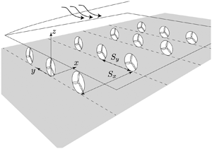
Inline and staggered wind-farm layouts were tested with different spacing and free stream turbulence in the present experimental campaign. Figure 3 shows a schematic representation of a farm together with the used reference frame while table 1 reports some details of the seven investigated test cases.
Schematic representation of an investigated wind farm and of the used reference frame. The farm canopy top plane  $z=z_0$ is indicated together with the internal boundary layer developing over the farm.

Characteristic parameters of the studied wind farms.

All cases have the same lateral turbine spacing, while in the staggered cases the even rows are shifted by  $1.5D$ sideways: the number of turbines is approximately the same as farm I, but the arrangement is more homogeneous. The resulting mean flow is shown at some streamwise cross-sections in figure 4 for farms I and III, where it can be noted that for the staggered configuration the flow is more homogenous in the spanwise direction.
Selected planes of the streamwise mean velocity field,  $U/U_{inlet}$, for farm I ( $a$) and III ( $b$).
$b$).

Figure 4 underlines that, while the staggered case is sufficiently homogenous to be studied as two-dimensional, the inline case is not since a large momentum deficit is concentrated in the wake of the line of turbines and 19 rows are not sufficient to merge it with the wake of neighbouring lines. It is expected that real wind farms, characterised by larger atmospheric turbulence, should have wakes that expand faster (as for instance in the well known picture of the Horns Rev farm), but nevertheless this lack of spanwise homogeneity will be solved by means of the horizontal average described in § 2.
The presence of the internal boundary layer above the farm was associated with the acceleration of the free stream above the farm (as the test-section ceiling was not changed): all cases are indeed subjected to a maximum 6 % increase of the free stream velocity between the leading edge and the trailing edge of the farm. This increase did not play a relevant role in the integral analysis of the velocity field, as discussed in § 4.2.
4. Results
The analysis of the database has been driven by the integral equations and by the attempt to build a simplified model based on the self-similarity of the velocity profiles. Dynamical features such as structures characterised by means of spectral analysis will also be discussed. All the data have been scaled with a reference inlet velocity  $U_{inlet}=8\ \textrm {m}\ \textrm {s}^{-1}$ and the figures will not report further this normalisation, unless stated otherwise. The Reynolds number calculated as ${Re} = D U_{inlet}/{\nu } \approx 24\,000$ is the same for all the present experiments.
4.1. Internal boundary-layer evolution
Figure 5 shows the spatially averaged mean velocity distribution in the streamwise and vertical directions for farm I. The streamwise mean velocity indicates a clear growth of an internal boundary layer over the farm until the farm trailing edge, after which the boundary layer is replaced by a developing wake. The leading edge of the farm induces an upward flow motion that ceases approximately near the farm trailing edge, where a fast downward motion is present.
Filtered mean velocity fields for farm I: ( $a$)
$a$)  $\left \langle U\right \rangle$ and ( $b$)
$b$)  $\left \langle W\right \rangle$

Despite the length of the farm, the vertical velocity did not become zero on top of the farm and the streamwise velocity decreases monotonically and does not show any indication of a plateau as observed in the experiments of Chamorro et al. (Reference Chamorro, Arndt and Sotiropoulos2011), Bossuyt et al. (Reference Bossuyt, Howland, Meneveau and Meyers2017, Reference Bossuyt, Meneveau and Meyers2018) and in the large eddy simulation results of Stevens et al. (Reference Stevens, Gayme and Meneveau2014, Reference Stevens, Gayme and Meneveau2016). This result is illustrated in figure 6 where the velocity in the axial and vertical directions at  $z=z_0$ are reported for farms I, II and III: with the exception of the farm trailing edge, the velocity is monotonically decreasing, while it increases again near the end of the farm due to the wake recovery in the farm wake and slightly upstream. This fact was also noted by Wu & Porté-Agel (Reference Wu and Porté-Agel2017) who found that under a weak stratification the flow in large wind farms, for both staggered and aligned cases, gradually decelerates as it enters the wind farm and does not reach a fully developed regime.
Averaged mean velocity in the streamwise ( $a$) and vertical ( $b$) direction at $z=z_0$ for farms I (solid line), II (dashed–dotted line) and III (dashed line).

Overall, the mean velocity shows a larger decrease in the staggered farm case than the inline one (similar to the results shown by Porté-Agel, Lu & Wu (Reference Porté-Agel, Lu and Wu2014), Wu & Porté-Agel (Reference Wu and Porté-Agel2017) and Sharma et al. (Reference Sharma, Cortina, Margairaz, Parlange and Calaf2018)) On the other hand, the inline case with largest spacing,  $S_x$, shows the lowest decrease of the streamwise mean velocity and so the lowest internal boundary-layer height, as already reported by Porté-Agel et al. (Reference Porté-Agel, Lu and Wu2014).
The measured velocity variances and covariance  $\left \langle \overline {u'w'}\right \rangle$ are shown in figure 7. As expected, the $\left \langle \overline {{u'}^{2}}\right \rangle$ Reynolds stress is larger than $\left \langle \overline {{v'}^{2}}\right \rangle$ and $\left \langle \overline {{w'}^{2}}\right \rangle$, although the last two have similar magnitude within the internal boundary layer. The turbulent activity tends to become larger when proceeding downwind and achieves its maximum near the trailing edge of the farm after which a decaying turbulent wake is present. The latter concentrates mostly near the top of the turbine canopy as the region characterised by the largest mean shear (as indicated in figure 5), while the bottom edge of the turbine leaves a weak footprint visible in the shear stress as a local maximum.
Filtered velocity variances  $\left \langle \overline {{u'}^{2}}\right \rangle$ ( $a$),
$a$),  $\left \langle \overline {{w'}^{2}}\right \rangle$ ( $b$),
$b$),  $\left \langle \overline {{v'}^{2}}\right \rangle$ ( $c$) and covariance $\left \langle \overline {{u'w'}}\right \rangle$ ( $d$) for farm I. All covariances are multiplied by a factor 1000 for the sake of clarity.

As a result of the spatial averaging procedure, new unknown terms appear in the filtered equations related to the spatial variation of the time-averaged quantities. These are the dispersive stresses reported in figure 8. These are expected to be relevant only in the presence of large variations of the mean field, namely near the turbines: since the region below the turbine canopy top was not measured, it is hard to estimate their value or relevance there, but some indication about their importance comes from the wake measurements after the farm trailing edge, where the highest magnitude of the dispersive normal stresses is located. Another region where large dispersive stresses are concentrated is along the farm edge, as visible in  $\left \langle U''^{2}\right \rangle$ and $\left \langle U''W''\right \rangle$.
Filtered dispersive stresses  $\left \langle U''^{2}\right \rangle$ ( $a$),
$a$),  $\left \langle W''^{2}\right \rangle$ ( $b$),
$b$),  $\left \langle V''^{2}\right \rangle$ ( $c$),
$c$),  $\left \langle U''W''\right \rangle$ ( $d$) for farm I. The dispersive stresses are multiplied by a factor 1000 for the sake of clarity.

It is important at this point to compare the dispersive stresses with the Reynolds stresses in order to assess their role in the generation of the vertical flux of kinetic energy. Figure 9 shows the comparison between Reynolds stresses and dispersive stresses near the farm top, i.e. at  $z=z_0$: the dispersive stresses are in general smaller than the Reynolds stresses except for $\langle U''^{2}\rangle (z_0)$ that is comparable with $\langle \overline {u'^{2}}\rangle (z_0)$ in the entry region of the farm, although sufficiently far from the edge it becomes negligible. The dispersive shear stress is negligible compared with the turbulent one, so that $r_{13}$ is dominated by the Reynolds shear stress and will be replaced by $\langle \overline {u'w'}\rangle$ in the next sections.
Filtered Reynolds and dispersive stresses at  $z=z_0$ for farm I. The black lines indicate the Reynolds stresses while the red lines mark the dispersive stresses. ( $a$) Comparison between $\left \langle \overline {{u'}^{2}}\right \rangle$ and $\left \langle U''^{2}\right \rangle$ (solid line), $\left \langle \overline {{w'}^{2}}\right \rangle$ and $\left \langle W''^{2}\right \rangle$ (dashed line), $\left \langle \overline {v'^{2}}\right \rangle$ and $\left \langle V''^{2}\right \rangle$ (dotted line). ( $b$) Comparison between $\left \langle \overline {u'w'}\right \rangle$ and $\left \langle U''W''\right \rangle$. The stresses are multiplied by a factor 1000 for the sake of clarity.

4.2. Shear stress and vertical flux of kinetic energy
The velocity field can be better analysed by integrating the momentum conservation equation obtaining the von Kármán equation (2.7). The various terms in the equation have been calculated and plotted in figure 10 along the streamwise coordinate. By analysing the dominant terms, the turbulent shear stress above the wind farm can be estimated as
 \begin{equation} -\langle\overline{u'w'}\rangle(z_0) \approx U_e^{2}\frac{\mathrm{d}\theta}{\mathrm{d}\kern0.7pt x}- W_0\left( U_e - U_0 \right). \end{equation}
Budget of the von Kármán equation (2.7) estimated from the measurements performed for farm I: residual (blue),  $U_e^{2}{\mathrm {d}\theta }/{\mathrm {d}\kern0.07pt x}$ (red), $- W_0( U_e - U_0 )$ (green), $-r_{13}(z_0)$ (orange), $\delta ^{*}U_e{\mathrm {d}U_e }/{\mathrm {d}\kern0.07pt x}$ (purple), $-{\partial }/{\partial x}\int _{z_0}^{z_f}(r_{11}-r_{33})\,\mathrm {d}z$ (black) and ${\mathrm {d}}/{\mathrm {d}\kern0.07pt x}\int _{z_0}^{z_f}k_e\,\mathrm {d}z$ (brown). The $W_0$ used is the experimentally measured one.

Equation (4.1) is an important simplified relation between the turbulent shear stress, the momentum flux linked to the vertical velocity and the growth of the internal boundary layer expressed in terms of momentum thickness,  $\theta$. The external velocity, $U_e$, can be taken out of the derivative because its variation along the streamwise direction is negligible compared with the variation of $\theta$.
As indicated in figure 10, the residual of the von Kármán equation is comparable with the dominant terms. This is most likely due to a measurement error of the mean vertical velocity,  $W$, that is hard to measure compared with the streamwise velocity. The von Kármán equation can be instead used to compute the mean vertical velocity, $W_0$, that will be used in the following analyses: the vertical velocity calculated from (4.1) differs from the measured one by at most $1 \ \textrm {cm}\ \textrm {s}^{-1}$, a discrepancy well within the experimental uncertainty of the averaged vertical velocity. The use of the vertical velocity calculated from the von Kármán equation in the integrated energy equation (2.9) allowed us to make the residual of the energy equation smaller for all the investigated layouts.
The various terms of the integrated energy equation for farms I, II and III (2.9) are reported in figure 11 where the near balance between the transport term in the streamwise and vertical directions is evident. The third term playing a meaningful role is the dissipation that transfers energy from the mean flow to the turbulent one.
Budget of the integrated energy equation (2.9) estimated from the measurements performed for farms I (solid line), II (dashed–dotted line) and III (dashed line). Residual (blue line), transport along  $x$ (green line), transport along $z$ (red line) and dissipation term (orange line). The $W_0$ is the one obtained from the von Kármán equation (2.7).

The assumptions made in § 2.1 about the dominant terms of the energy equation are supported by the detailed budget shown in figure 12, where the various terms of the simplified energy equation (2.14) for farms I and III are plotted: the residual of (2.14) is within experimental uncertainty. By using the assumptions made about the small order of magnitude of the dispersive stresses above the farm and the near constancy of the external velocity,  $U_e$, (2.14) can be rewritten as
 \begin{equation} {-}U_0\langle\overline{u'w'}\rangle(z_0) + W_0\frac{\left( U_e^{2} - U_0^{2} \right)}2 = U_e^{3}\frac{\mathrm{d}\delta_e}{\mathrm{d}\kern0.7pt x} + \int_{z_0}^{z_f}\langle\overline{u'w'}\rangle\frac{\partial\langle U\rangle}{\partial z}\,\mathrm{d}z. \end{equation}
Equation (4.2) shows an interesting relation between the entire vertical flux of MKE  $P_{flux} = -U_0\langle \overline {u'w'}\rangle (z_0) + W_0( U_e^{2} - U_0^{2} )/2$ and the boundary-layer evolution over the wind farm expressed in terms of energy thickness, which is connected with the global deficit of kinetic energy flux along the streamwise direction in the internal boundary layer. The energy flux is not dominated just by the first term (as usually assumed in other studies, such as in Cal et al. (Reference Cal, Lebrón, Castillo, Kang and Meneveau2010) and Calaf et al. (Reference Calaf, Meneveau and Meyers2010)), but instead the transport of energy imparted by the vertical velocity is equally important as the turbulent flux especially for the inline case.
Budget of the simplified integrated energy equation (2.14) estimated from the measurements performed for farms I (a) and III (b). Residual (blue line), internal boundary layer growth  $U_e^{3}{\mathrm {d}\delta _e}/{\mathrm {d}\kern0.07pt x}$ (green line), vertical flux of kinetic energy (red line) and dissipation term (orange line). The vertical flux is decomposed in the turbulent component $U_0\langle \overline {u'w'}\rangle (z_0)$ (dashed line) and in the component linked to the vertical mean velocity $-W_0( U_e^{2} - U_0^{2} )/2$ (dash–dotted line).

According to (4.2), the evolution of the energy thickness,  $\delta _e$, is associated with the energy flux. It is indeed interesting to study the evolution of the characteristic thicknesses of the internal boundary layer above the farm. Figure 13 shows the three thicknesses $\delta ^{*}$, $\theta$ and $\delta _e$ together with $\delta _{95}$ (representing the boundary-layer thickness as the distance between $z_0$ and the height where the velocity $U$ is equal to $0.95U_{e}$) for farms I and III. It is clear that the boundary layer grows nearly linearly from $x\approx 15D$ (approximately after three to four rows where there is a change in the concavity), and it grows faster for the staggered layout although with a larger virtual origin: the concavity change implies a change of dominant dynamics between the initial stage (driven by the pressure gradient) and the following stage and a shift of the virtual origin in the internal boundary-layer evolution. The shape factor $H = \delta ^{*}/\theta$ is not constant but it grows nearly linearly from 1.05 at $x/D=10$ to 1.25 at $x/D=70$. In light of this change, no parallel state is achieved and the velocity profile is not self-similar.
Streamwise distribution of several boundary-layer thicknesses (normalised by the turbine diameter) for farms I (solid lines) and III (dashed lines).

It is interesting at this point to analyse the turbulence-induced vertical flux of MKE,  $-U_0\langle \overline {u'w'}\rangle (z_0)$, in all the layouts available. These are shown in figure 14: a growing trend is generally visible, similar to the results of Cortina et al. (Reference Cortina, Sharma, Torres and Calaf2020). The case with the lowest flux is farm II, corresponding to a reduced turbulent activity within the internal boundary layer: this implies that the magnitude of the kinetic energy entrainment from the free atmosphere into the boundary layer increases by increasing the density of the farms, as already shown by Porté-Agel et al. (Reference Porté-Agel, Lu and Wu2014) and Wu & Porté-Agel (Reference Wu and Porté-Agel2017). The energy flux is also enhanced by the free stream turbulence that is beneficial from the energy production point of view since the flux replenishes more energy within the farm. It is interesting to note that a transition in the turbulent flux is present when free stream turbulence is present for the inline case: farms I, IV and V start similarly at the beginning of the farm but the free stream turbulence enhances the turbulent flux later on, an enhancement that takes place earlier for larger free stream turbulence structures. This is particularly unexpected as both grids were associated with similar statistics and integral time scales (as shown in figure 1).
Turbulence-induced vertical flux of MKE,  $-U_0\langle \overline {u'w'}\rangle (z_0)$: farms I (solid black line), II (solid grey line), III (dashed line), IV (triangles with solid line), V (circles with solid line), VI (triangles with dashed line) and VII (circles with dashed line).

By analysing the entire vertical flux of MKE (i.e. the sum of the turbulent flux and the vertical velocity displacement of MKE) for the available layouts, one obtains an interesting result: as visible in figure 15, the value of the flux along the farm is roughly the same for the different staggered layouts (with or without free stream turbulence) for a significant length of the farm and it is approximately  $P_{mean} \approx 0.0051U_{inlet}^{3}$. It is generally lower for inline layouts (lowest for farm II), as expected, and oscillates around a value of $P_{mean} \approx 0.0040U_{inlet}^{3}$, which might suggest that in large wind farms the staggered configuration is more efficient, due to a longer distance to recover the velocity deficit between consecutive turbine rows compared with inline farms (Chamorro & Porté-Agel Reference Chamorro and Porté-Agel2011; Chamorro et al. Reference Chamorro, Arndt and Sotiropoulos2011; Archer, Mirzaeisefat & Lee Reference Archer, Mirzaeisefat and Lee2013; Porté-Agel et al. Reference Porté-Agel, Lu and Wu2014; Bossuyt et al. Reference Bossuyt, Howland, Meneveau and Meyers2017; Wu & Porté-Agel Reference Wu and Porté-Agel2017). The average flux accounts also for the region near the leading and trailing edge of the farm where the flux is generally lower. This is in direct contrast with figure 14 where the turbulent flux grows almost monotonically, highlighting the important role of the vertical transport of kinetic energy in these special regions and underlining the decreasing trend of the flux of energy correlated with the mean vertical velocity, $W_0$. In the last two rows, the vertical energy flux is provided only to the turbulent energy flux, similar to what happens in an infinite farm.
Vertical flux of MKE,  $P_{flux}$, for the available layouts. See figure 14 for the used list of symbols: mean value of the flux for the staggered layouts (dashed red line), mean value of the energy flux for the inline layouts with $S_x = 4D$ (solid red line).

4.3. Self-similar analysis
From the analysis of the shape factor it was evident that the mean velocity profile is not self-similar. However, the mean velocity profile can be analysed in terms of deficit  $U_e - \langle U\rangle (z)$ and scaled with the characteristic velocity scale $U_e - U_0$. In case of self-similarity, it is expected that the profile could be described by a function of $(z-z_0)/\delta _{20}$ where $\delta _{20}$ is the position where $U_e - \langle U\rangle (\delta _{20}) = 0.2(U_e -U_0)$. Figure 16 $(a)$ shows the mean velocity profile for farm I at different streamwise positions, while figure 16 $(b)$ shows the mean velocity profiles at $x/D$ = 30 for the available layouts. An evident collapse of the data is observed in both figures supporting the self-similarity of the mean velocity deficit profile above the wind farm. The curve of the profile can be represented by the error function defined as $1-\mathrm {erf}[a(z-z_0)/\delta _{20}]$ for $a=0.9062$ (calculated by imposing that the function is 0.2 for $(z-z_0)/\delta _{20}=1$).
Mean velocity profile for different streamwise positions for farm I ( $a$) and for different layouts at $x/D=40$ ( $b$). In panel ( $a$) the red markers indicate the profile for $5< x/D<15$, the green markers for $20< x/D<55$ and the blue markers for $60< x/D<70$; $1-\mathrm {erf}(a(z-z_0)/\delta _{20})$ (Solid line).

A worse agreement of the data is instead observed for the Reynolds shear stress profile,  $\langle \overline {u'w'}\rangle$, scaled with the local friction velocity defined as the maximum shear stress along $z$. The normalised shear stress profile is reasonably described by a function of $(z-z_0)/\delta _{20}$ sufficiently downwind of the farm leading edge, as visible in figure 17. A change in concavity is clearly present near the farm canopy top, highlighting, however, that a two-scale structure would better describe the shear stress profile, although there is no footprint of that in the mean velocity profile. By observing the velocity and the shear stress profile, both present a better agreement in the middle of the farm (green markers) because there are no sensible effects due to the leading and the trailing edge of the farm. The account of the dispersive shear stress did not improve the agreement between the profiles at different streamwise stations or layouts.
Reynolds shear stress profile for different streamwise positions for farm I ( $a$) and for different layouts at $x/D=40$ ( $b$). In panel ( $a$) the red markers indicate the profile for $5< x/D<15$, the green markers for $20< x/D<55$ and the blue markers for $60< x/D<70$.

According to the previous analyses, there is a relation between the mean velocity deficit profile above the farm, the evolution of the internal boundary layer in terms of  $\delta _{20}$ and the mean velocity at $z_0$, $U_0$, of the form
 \begin{equation} \frac{U_e-\langle U\rangle}{U_e-U_0} = f\left(\frac{z-z_0}{\delta_{20}}\right). \end{equation}
By using the velocity profile  $\langle U\rangle (z)$ with the relation (4.3), the characteristic thicknesses (and therefore the vertical flux of kinetic energy being related to the growth of $\delta _e$) can be expressed as a function of these two parameters, i.e. $P_{flux} = P_{flux}( U_0, \delta _{20})$. The evolution of $\delta _{20}$ can be estimated from internal boundary-layer growth considerations as $\delta _{20} \approx c(x-x_0)^{4/5}$ (Meneveau Reference Meneveau2012), where $c$ and $x_0$ are two parameters that depend on the layout of the farm. In the particular example of farm I, the best parameters that interpolate the data are $c=0.05$ and $x_0/D=2.5$.
Although not related to a self-similar analysis, it is interesting to have a look at the diagnostic plots (Alfredsson et al. Reference Alfredsson, Segalini and Örlü2011) for the streamwise and spanwise velocity variance, shown in figure 18. These plots use the streamwise mean velocity profile as independent coordinate instead of  $z$. There is reasonable agreement for the same layout at different streamwise locations for the streamwise and spanwise normal stress, especially for the inline cases (the scatter is reduced there if the profiles at $x/D=20$ and 60 were removed). From case to case there is, however, variability that could be explained with a different roughness function (as discussed by Castro, Segalini & Alfredsson (Reference Castro, Segalini and Alfredsson2013)), although the estimation of the roughness function was not attempted here since the logarithmic region (if present) should not be relevant compared with the outer function in the internal boundary layer. Inline layouts have a general higher variance than staggered layouts and the free stream turbulence enhances the variance even more. Farm II has a turbulence intensity distribution comparable to the inline cases with $S_x=4D$, although the mean velocity deficit is reduced (as well as the variance profile). It is also worth mentioning that the inclusion of the dispersive stresses worsened significantly the agreement of the streamwise normal stresses, underlining that the diagnostic-plot analysis should be just related to the velocity variances rather than the total stresses.
Scatter plots of the Reynolds stresses  $\langle \overline {{u'}^{2}}\rangle ^{1/2}$ and $\langle \overline {{v'}^{2}}\rangle ^{1/2}$ against the local mean velocity at $x/D=20,\,30,\,40,\,50,\,60$ for the inline farms ( $a$,
$a$, $b$) and staggered farms ( $c$,
$c$, $d$): clean cases (blue), grid cases with $M/D=0.56$ (red), grid cases with $M/D=1.11$ (black solid lines), farm II (green). The black dashed line indicates the streamwise Reynolds stress relationship of Alfredsson et al. (Reference Alfredsson, Segalini and Örlü2011).

4.4. Spectral analysis
The mean velocity field and the energy flux have been analysed in the discussions above. In order to understand the dynamical behaviour of the velocity field above a wind farm, a spectral analysis has been performed providing the energy distribution at the different scales of the turbulent motion. The power spectral density of the velocity time series at each measurement point was computed and it was spatially averaged for each frequency obtaining the averaged frequency spectrum,  $\langle S_{uu}\rangle (x,\,z,\,f)$. All the spectra not normalised by the variance are multiplied by a factor 1000 for the sake of clarity.
Figure 19 shows the frequency spectrum map as a function of  $x/D$ and of the non-dimensional frequency ${St} = f D/U_0$ for $z=z_0$. A characteristic frequency above the farm is visible throughout the farm length with a value of ${St}\approx 0.15$, although with a decreasing trend with $x$. This frequency is different from the tip-vortex frequency (located at ${St}=1.7$) clearly visible and relevant only near the leading edge of the farm, after which the wake becomes too turbulent and the tip vortices lose their coherency and strength. The large difference between the characteristic frequency observed downwind and the tip-vortex frequency suggests that the former is associated with a different phenomenon: the broadband distribution indicates a turbulent nature such as the wake meandering observed behind wind turbines (Medici & Alfredsson Reference Medici and Alfredsson2006; España et al. Reference España, Aubrun, Loyer and Devinant2012; Coudou et al. Reference Coudou, Buckingham and van Beeck2017). The Strouhal number appears to be of the same order of the one observed in the literature about wake meandering (Medici & Alfredsson Reference Medici and Alfredsson2006) although a bit lower since $U_0$ is expected to be higher than the velocity at hub height.
Premultiplied streamwise velocity spectrum map,  $f\langle S_{uu}\rangle$, as function of $x/D$ and ${St}$ for $z=z_0$ for farm I.

Wake meandering is a transversal fluctuation of the wake downwind of wind turbines and therefore the wake meandering should be visible even in the non-premultiplied spectrum  $\langle S_{vv}\rangle$. Figure 20 shows $\langle S_{vv}\rangle$ at $z=z_0$ and different streamwise positions where the presence of a peak is evident: the Strouhal number (intensity) of the peak is decreasing (increasing) with the streamwise distance. Figure 21 shows the corresponding evolution of the premultiplied spectra of the streamwise velocity (the spanwise velocity exhibited more of a plateau there) at $z=z_0$: the premultiplied spectra change in frequency and magnitude along the streamwise direction with turbulent structures that become bigger and more energetic by travelling downwind.
Transverse velocity spectrum for  $z=z_0$ and for $x/D=15,\,30,\,45,\,60$ for farm I.

Streamwise velocity spectra for  $z=z_0$ and for $x/D=15,\,30,\,45,\,60$ for farm I; ${St}^{-2/3}$ (dashed line).

Figure 22 shows the comparison of the dominant Strouhal number detected from the premultiplied spectra  $f\langle S_{uu}\rangle$ for all the available farms: despite the different layouts, turbine distance and free stream turbulence state, the Strouhal number appears to approach a general trend quite rapidly after the first rows, highlighting once again how the wake meandering dominates the turbulent large-scale dynamics in deep arrays and it should be therefore considered as the leading dynamical phenomenon in a large farm that builds up already after the first two to three rows of turbine. The coupling between atmospheric turbulence and this kind of motion is also quite intriguing: in the present experiment the upstream flow is not characterised by large-scale turbulent motions without a grid, and therefore the results should miss the dynamical wake meandering mechanism driven by large-scale motions (Larsen et al. Reference Larsen, Madsen, Thomsen and Larsen2008; Braunbehrens & Segalini Reference Braunbehrens and Segalini2019). However, if the farm is sufficiently long, large-scale structures are generated internally anyhow and the Strouhal number agreement of figure 22 shows that the route is the same regardless of the free stream turbulence activity. Therefore, models that do not account for self-generated large-scale structures might actually wrongly estimate the meandering dynamics and its effect on turbine loads.
Comparison of the Strouhal number associated with the peak of the premultiplied streamwise velocity spectrum. See figure 14 for the list of symbols used.

The decreasing trend of the Strouhal number suggests a modulation of the dominant dynamical phenomenon: as the internal boundary layer grows along the farm, it is expected that the turbulent structure's size should increase with  $x$ as more space is available. In order to support this, figure 23 shows that, when the Strouhal number is obtained by using the distance $z_0+\delta _{95}$ (i.e. the distance between the ground and the internal boundary-layer edge), a nearly constant value is obtained that weakly depends on the farm layout (the most significant deviation is for farm II with large spacing between the turbines).
Comparison of the Strouhal number scaled with the wake size,  $z_0+\delta _{95}$. See figure 14 for the list of symbols used.

The velocity spectra agree reasonably well if they are scaled by the velocity variance and the integral time scale,  $\langle \varLambda _u\rangle$, as shown in figure 24. It is evident that the spectra are indeed described by a universal function in the normalised frequency and no structural change takes place over the farm. The same agreement is visible for the spectra of the other velocity components and the cross-spectra as well. The agreement of the spectra implies again a tight connection between the integral time scale and the size of the wake $z_0+\delta _{95}$.
Normalised frequency spectrum for  $z=z_0$ and for $x/D=15,\,30,\,45,\,60$ for farm I: ${f}^{-2/3}$ (dashed line).

A final consideration can be done about the structure of the spectra long downwind the farm leading edge. Figure 25 shows the low frequency part of the spectra of the three velocity components for two inline farms (I and II) and one staggered farm (III). They are all dominated by the streamwise component that is more energetic than the other two, especially at the largest scale. The spanwise and vertical velocity components start to have increasing relevance near the large scale peak of  $f\langle S_{uu}\rangle$ and they even exceed $f\langle S_{uu}\rangle$ for large frequencies: interestingly, they approach the value of $4/3S_{uu}$, i.e. the isotropic turbulence state (Segalini & Arnqvist Reference Segalini and Arnqvist2015) for a short range, and remain above this theoretical expectation for the rest of the inertial range.
Premultiplied velocity spectra at  $x/D=40$ and $z=z_0$ for farms I ( $a$), II ( $b$) and III ( $c$):
$c$):  $S_{uu}$ (blue solid line), $S_{vv}$ (red line), $S_{ww}$ (black line), $4S_{uu}/3$ (blue dashed line).

5. Conclusions
An analysis of the internal boundary-layer evolution over several long farms has been proposed in the present work. Inline and staggered layouts with and without free stream turbulence have been characterised in detail above the turbine canopy in order to quantify the flux of energy replenishing the energy available to the turbines and to characterise the evolution of the internal boundary layer. Hot-wire measurements have been performed providing time-resolved data for the computation of velocity statistics and spectra. The data have been space-averaged to remove the turbine-to-turbine variations enabling a boundary-layer analysis from the spatially filtered Navier–Stokes equations and removing the need of a complex three-dimensional analysis.
The analysis indicated that an internal boundary layer is generated above the turbine canopy that grows monotonically until the end of the farm. Within this layer, the velocity deficit and the turbulence intensity keep growing, implying a lower velocity and higher turbulence experienced by the downwind turbines, as expected. The boundary layer is characterised by an enhanced turbulent activity that transfers momentum below the turbine canopy together with the appearance of dispersive stresses due to the spatial averaging: the latter are mostly smaller than the associated Reynolds stress with the exception of  $\langle {U''}^{2}\rangle$ and $\langle {U''W''}\rangle$ very close to the turbine canopy top and entry region of the farm.
The integrated momentum and energy equations provided a framework to analyse the velocity data in terms of momentum balance and energy flux: it was found that the latter is composed of a turbulent energy flux (proportional to the Reynolds stress and the local momentum) and an advection term related to the kinetic energy transported by the vertical velocity. The former term has been discussed in previous analyses of wind-farm flows and it is the only one present in the infinite-farm case. However, the latter has here been found to be equally important as the turbulent flux throughout the entire length of the farm especially for the inline layouts and therefore it cannot be neglected if an estimation of the total energy flux is desired such as, for instance, in ‘top-down’ models. The energy analysis pointed out the dominant balance between the vertical energy flux and the growth of the energy boundary layer, with a weak dissipative term transferring energy from the mean to the turbulent field. This implies that an assessment of the evolution of the mean flow would be sufficient to estimate the energy flux throughout the farm canopy top.
A self-similar analysis of the velocity profile indicated that the mean velocity deficit profile is self-similar and scales with the velocity deficit on top of the farm and with a characteristic thickness based on the velocity deficit profile. The shear stress profile seems to follow a similar scaling although with a slightly worse agreement, suggesting a more complex structure. The use of the diagnostic plot (Alfredsson et al. Reference Alfredsson, Segalini and Örlü2011) highlighted a connection between the mean velocity and the velocity variances that is weakly affected by the farm layout, similar to rough-wall turbulent boundary layers (Castro et al. Reference Castro, Segalini and Alfredsson2013). The free stream turbulence appears to enhance the turbulent fluctuations compared with the case with non-turbulent flow, so that the internal boundary layer is indeed modulated by the presence of an enhanced vortical activity outside that.
A spectral analysis indicated that the dominant dynamical phenomenon along the farm is the meandering of the turbine wakes, a dynamics that builds up already after the first two to three rows of turbine and that overwhelms the tip-vortex signature observed only behind the first row of turbines and that looses abruptly coherence and strength due to the turbulent environment. A Strouhal number of the wake meandering of approximately  ${St}=fD/U_0\approx 0.15$ was observed although it is expected that a number closer to 0.2 (the observed wake meandering Strouhal number (Medici & Alfredsson Reference Medici and Alfredsson2006)) should be observed if the chosen reference velocity was the one inside the farm at hub height. The same Strouhal number has been observed for both inline and staggered layouts regardless of the free stream turbulence level with a similar trend along the streamwise direction, suggesting a universal dynamical feature. This trend was removed when scaling the Strouhal number with $z_0+\delta _{95}$ (i.e. the distance between the ground and the edge of the internal boundary layer), suggesting that the Strouhal number should change for sufficiently long wind farms that do not achieve a fully developed state.
Finally, the comparison of the spectra of the various velocity components for different farm layouts indicated that energy is provided at large scales to the streamwise velocity component, while the spanwise and vertical components become dynamically relevant near the peak of maximum energy of the streamwise component. After this, the energy in them exceed the one of the axial component as it should do in the inertial subrange in isotropic turbulence, although they tend to exceed the theoretical limit of  $S_{vv}=S_{ww}=4S_{uu}/3$, suggesting that anisotropy is still present even at the small scales of motion.
Acknowledgements
The authors wish to acknowledge J.-Å. Dahlberg at Vattenfall Vindkraft AB for manufacturing the wind-turbine rotors and A. Hyvärinen for the initial set-up of the experiment. A.S. is supported by the Swedish strategic research program STandUP for Wind.
Funding
The work presented in the present paper has been funded by the Swedish Research Council (VR) under a framework grant for strategic energy research.
Declaration of interests
The authors report no conflict of interest.
Data availability statement
The data that support the findings of this study are available upon request.
Author contributions
All authors contributed equally to analysing data and reaching conclusions, and in writing the paper.


 Open access

