

Introduction
Analysing the relevance of family background characteristics to individuals’ levels of income is important to understand how individuals’ income is determined by factors beyond their responsibility and, consequently, the extent to which a society is able to guarantee equal opportunities for all.
This article aims to analyse the role family background characteristics play in shaping individuals’ income and its subsequent effect on inequalities in Spanish regions. For this purpose, we get estimates of inequality for the Spanish regions and compute the importance of family background characteristics to the observed levels of income Additionally, we analyse the differences in inequality levels between the Spanish regions trying to disentangle the main drivers of the levels of inequality.
Ensuring equal opportunities in a society would mean that all individuals are able to achieve a certain level of income regardless of the level of income, wealth or education attained by their progenitors or any other circumstances beyond their own control. The analysis of equal opportunities in economics has been popularised by Roemer (Reference Roemer1993, Reference Roemer1998), following the work of several authors (Arneson, Reference Arneson1989; Cohen, Reference Cohen1989; Dworkin, Reference Dworkin1981a, Reference Dworkin1981b; Nozick, Reference Nozick1974; Rawls, Reference Rawls1971; Sen, Reference Sen1979), whose contributions incorporate the idea of equal opportunities from different perspectives.
Likewise, educational inequalities and income inequalities are closely related (Checchi and van de Werfhorst, Reference Checchi and van de Werfhorst2018; Palmisano et al., Reference Palmisano, Biagi and Peragine2022; Solga, Reference Solga2014) For instance, Solga (Reference Solga2014) found that education could be a great equalizer for income inequality when accompanied with redistributive policies. Furthermore, Checchi and van de Werfhorst (Reference Checchi and van de Werfhorst2018) find that inequality in the quality of education affects income inequality, indicating that their results are to some extent consistent with human capital and functionalist theories, which argue that education is rewarded because of the skills needed in the labor market, so inequality in the quality of education is expected to affect income inequality more. Palmisano et al. (Reference Palmisano, Biagi and Peragine2022) show that inequality of opportunity in education is strongly correlated with inequality of opportunity in income. The research available in this regard for Spain shows a strong relationship between the income and social class of the parent and the school performance of individuals (Bernardi and Cebolla, Reference Bernardi and Cebolla2014; Peraita and Pastor, Reference Peraita and Pastor2000).
Although there are some works that analyse income inequalities and mobility in Spain (Ayala and Jurado, Reference Ayala and Jurado2011; Budría and Moro-Egido, Reference Budría and Moro-Egido2008; Cabrera et al., Reference Cabrera, Marrero, Rodríguez, Salas-Rojo and Gabriel2021; Cantó, Reference Cantó2000; Pijoan-Mas and Sánchez-Marcos, Reference Pijoan-Mas and Sánchez-Marcos2010; Suárez Álvarez and López Menéndez, Reference Suárez Álvarez and López Menéndez2020) most of them study inequality before the year 2000. In this sense, it is important to perform an analysis with a more recent period in order to have a more adequate picture of the current reality, which will allow policy makers to carry out public policies that are more in line with current needs.
Likewise, the role of parental background in education has previously been analysed in several investigations in equality of opportunity. It has been proved that parental education and parental occupation are two of the most relevant circumstances in shaping individual outcome in income (Belhaj Hassine, Reference Belhaj Hassine2012; Bourguignon et al., Reference Bourguignon, Ferreira and Menéndez2007; Brunori et al., Reference Brunori, Hufe and Mahler2018; Pestieau, Reference Pestieau1989; Singh, Reference Singh2012; Suárez Álvarez and López Menéndez, Reference Suárez Álvarez and López Menéndez2018a, Reference Suárez Álvarez and López Menéndez2018b). Moreover, focusing on the Spanish case (Cabrera et al., Reference Cabrera, Marrero, Rodríguez, Salas-Rojo and Gabriel2021; Suárez Álvarez and López Menéndez, Reference Suárez Álvarez and López Menéndez2018a), found that parental education significantly affects individuals’ income.
Our objective is to analyse how different educational and family background variables at regional level are related to the observed levels of inequality. Inequalities and educational achievements can experience great variations between regions. In the Spanish case this fact could be especially relevant and interesting due to several reasons: (1) there are significant income inequalities between regions (2) the distribution of income growth among the population differs between regions and (3) the education systems are different since the competencies in education are shared by the Spanish regions and the central government, resulting in differences in the educational systems across regions.
To this end, the analyses carried out in this article try to answer two main questions: (1) To what extent are family background characteristics important in shaping inequalities? And (2) Which are the main drivers of inequalities across regions? We will consider inequalities in income, and for this purpose, we will use the disposable income of individuals as an outcome variable to measure both income inequality and inequality of opportunity.
Taking into account that Spanish regions are very different from one another, one could expect to find different answers to these questions depending on the region. In fact, Suárez Álvarez and López Menéndez (Reference Suárez Álvarez and López Menéndez2020) showed the importance of the regional dimension for the analysis of inequalities and opportunities. Therefore, we perform our analyses at regional level, considering the seventeen Spanish NUTS-II units (Autonomous Communities, CCAA). Likewise, since the analysis is at the regional level, it is important to note that there was no devolution of government responsibilities during the period under analysis.
The rest of the article is structured as follows. Section two presents the database and the variables used, also providing some descriptive statistics. Section three shows the estimates of inequality and inequality of opportunity for the Spanish regions and the contribution of different circumstances to the level of inequality of opportunity. Section four provides evidence on the main determinants of the different levels of inequality observed across regions, with a focus on educational variables. Finally, Section five summarises the conclusions of the article.
Database description
The analyses performed in this article rely on the European Survey of Income and Living Conditions (EU-SILC), a survey that contains datasets at individual and household level. Furthermore, data are classified by regions – in particular, EU NUTS-II regions, which correspond to the Spanish Autonomous Communities (CCAA). They are first level political and administrative divisions and each one has its own organic laws known as Statutes of Autonomy, which determine the powers they have. They are also divided into provinces (EU NUTS-III regions).
Specifically, in this article we use the EU-SILC surveys conducted in 2011 and 2019 which provide income variables referred to years 2010 and 2018. The use of these two surveys is particularly relevant since they include an ad-hoc module which incorporates variables regarding individuals’ family background.
Our analysis is focused on the seventeen Spanish Autonomous Communities and the sample is restricted to individuals aged twenty five to fifty nine years because parental background variables are only provided for individuals within this range of age.
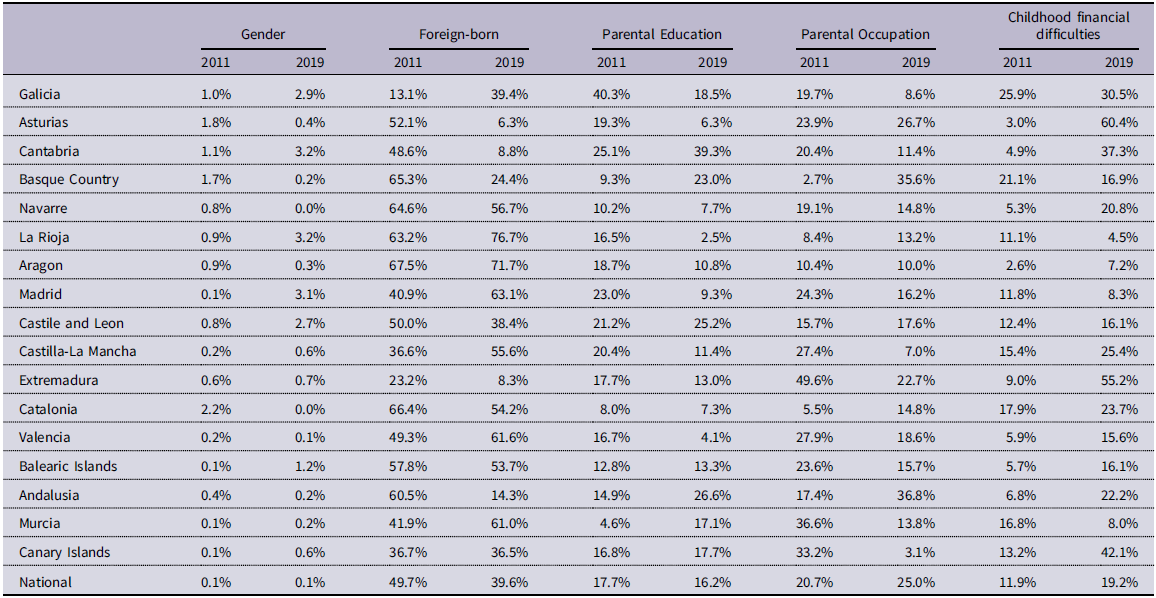
The variables we use refer to individuals’ circumstances, i.e. factors that are beyond individuals’ responsibility. For this purpose, we use variables regarding individuals’ family background when they were children. The first is Parental Education, which is constructed using the maximum level of education of both progenitors classified into three categories: low if both progenitors have at maximum a degree of compulsory education, medium, if at least one progenitor has completed secondary education and high, when at least one progenitor has completed tertiary education.
Similarly, we use the variable Parental Occupation, which refers to the occupation of individuals’ progenitor when they were children. This variable is also divided into three categories, according to the ISCO-08 jobs classification. More specifically, these three categories are low skilled when both parents work in elementary occupations (groups eight and nine of ISCO-88 classification), medium skilled when at least one parent works in an occupation comprised in groups five to seven of the classification and high skilled if at least one progenitor works in a high skilled occupation (groups one to four in ISCO-08)Footnote 1.
We also include the variable Childhood Financial Difficulties, which is a perception-based measure that considers respondent’s feeling about the financial situation of the family when the respondent is around fourteen years old. It is divided into four categories: Bad/very bad, Moderately bad, Moderately good and Good/very good.
The variables used as circumstances correspond to a period prior to the one for which the income of individuals is analysed. These variables correspond to the childhood period of the individuals, since the idea is that they provide an approximation of their social and family environment and that they are circumstances – that is, that they do not depend on the responsibility of the individuals and, clearly, individuals cannot occur to them due to situations that occurred during their childhood.
Finally, we include a variable referred to income, which will be used to measure inequality – we use the equivalised disposable income of households, which is equivalised by considering the structure of each household. Specifically, this variable is constructed according to the equivalence scale used by EU-SILC, which is the Organisation for Economic Cooperation and Development (OECD)-modified scale:
 $e = 1 + 0.5\left( {{N_{{{14}^ + }}} - 1} \right) + 0.3{N_{{{13}^ - }}}$
where
$e = 1 + 0.5\left( {{N_{{{14}^ + }}} - 1} \right) + 0.3{N_{{{13}^ - }}}$
where
 ${N_{{{14}^ + }}}$
is the number of household members who are over fourteen years and
${N_{{{14}^ + }}}$
is the number of household members who are over fourteen years and
 ${N_{{{13}^ - }}}$
the number of members who are thirteen or younger.
${N_{{{13}^ - }}}$
the number of members who are thirteen or younger.
The equivalised disposable income is considered a good proxy of the available income individuals have. In addition, this variable has been used in other studies with EU-SILC data referred to education and inequalities – such as Brzezinski, Reference Brzezinski2015; Marrero and Rodríguez, Reference Marrero and Rodríguez2012; Palomino et al., Reference Palomino, Marrero and Rodríguez2016; Suárez Álvarez and López Menéndez, Reference Suárez Álvarez and López Menéndez2018b, Reference Suárez Álvarez and López Menéndez2018a.
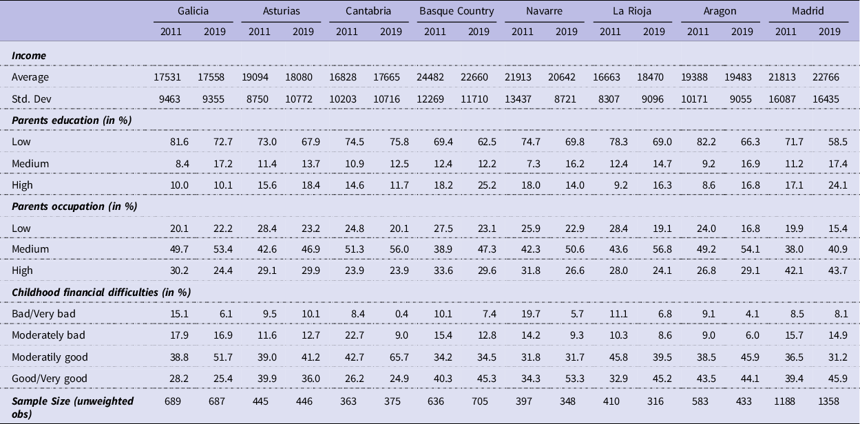
Table 1 provides a summary of the descriptive statistics at the regional level and for the two years analysed, 2011 and 2019. More specifically, it shows the share of the population within each category of the above-mentioned variables.
Main descriptive (part 1)

Main descriptive (part 2)
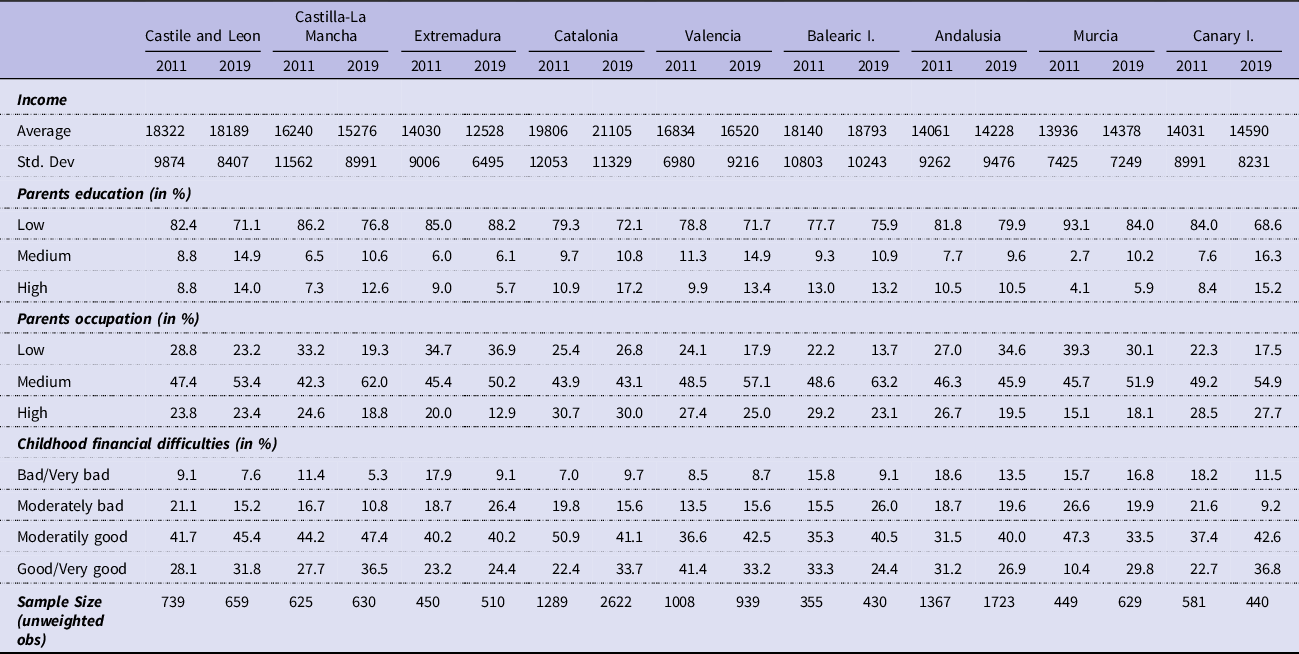
Additionally, Table 1 shows the sample size for each region and year. It can be noticed that in some regions the sample size is not very large, the survey used (EU-SILC) provides weights to make the results representative. Nevertheless, caution is advised when interpreting the results.
Estimating inequality of opportunity
This Section is devoted to estimate income inequality and inequality of opportunity (IOp) and to compute the contribution of the variables used to circumstances to IOp with the aim of showing at what extent family background characteristics and other circumstances are affecting individuals’ performance in terms of income.
For this purpose, in addition to estimating income inequality, we compute inequality of opportunity (IOp henceforth) for the Spanish regions and then we analyse the contribution of the variables used as circumstances to this indicator.
The basis of the study of IOp can be found in Roemer (Reference Roemer1993) and Yitzhaki and Schechtman (Reference Yitzhaki and Schechtman2013); later on Roemer (Reference Roemer1998) formalise this concept and distinguish between circumstances, understood as factors beyond individuals’ control, and efforts, that can be attributed to individuals’ performance and commitment. In this context, the analysis of IOp tries to compute the part of inequality due to the first kind of factors, in which parental background characteristics are included.
To know the effect that parental background characteristics have in inequality and more specifically in inequality of opportunity, we estimate the indices of both sorts of inequalities for each of the seventeen Spanish regions analysed before computing the contribution of these characteristics.
Firstly, to estimate IOp, in addition to previous variables referring to individuals’ family background, we include two more variables regarding individuals’ personal circumstances in order to obtain reliable estimates and reduce the omitted variables bias. These two variables are: Gender, with two categories, female and male and Country of birth with two categories Foreign-born persons and Spanish-born.
To estimate IOp we use the ex ante parametric method (Ferreira and Gignoux, Reference Ferreira and Gignoux2011), although there are many other alternative methodologies (see Ferreira and Peragine, Reference Ferreira and Peragine2015; Ramos and Van de Gaer, Reference Ramos and Van de Gaer2016; Roemer and Trannoy, Reference Roemer and Trannoy2016). We have decided to use the ex-ante parametric method since this is the most widely used procedure in the IOp literature and thus allows comparability with other studies. Furthermore, this method has the additional advantage that it does not require including information referred to the level of effort.
In order to compute IOp we divide individuals into types
 $T$
, being each type formed by individuals that share the same categories of each circumstantial variable. In our case we have five variables Parental Education, Parental Occupation, Childhood Financial Difficulties, Gender and Country of birth with three, three, four, two and two categories each, thus leading to a total of 144 different types of individuals. These are the variables considered to be beyond individuals’ responsibility and therefore treated as circumstances.
$T$
, being each type formed by individuals that share the same categories of each circumstantial variable. In our case we have five variables Parental Education, Parental Occupation, Childhood Financial Difficulties, Gender and Country of birth with three, three, four, two and two categories each, thus leading to a total of 144 different types of individuals. These are the variables considered to be beyond individuals’ responsibility and therefore treated as circumstances.
Then, we estimate individual incomes following the expression:
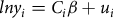 $ln{y_i} = {C_i}\beta + {u_i}$
, where
$ln{y_i} = {C_i}\beta + {u_i}$
, where
 ${C_i}$
denotes the different variables used as circumstances and
${C_i}$
denotes the different variables used as circumstances and
 $\beta $
represents the effect these circumstances have on income. Once the equation is estimated we get the fitted values:
$\beta $
represents the effect these circumstances have on income. Once the equation is estimated we get the fitted values:
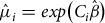 ${\hat \mu _i} = exp\left( {{C_i}\hat \beta } \right)$
which are a counterfactual distribution of income that depends only on the circumstances. (Tables A1 and A2 in the Appendix section show the results of the regressions).
${\hat \mu _i} = exp\left( {{C_i}\hat \beta } \right)$
which are a counterfactual distribution of income that depends only on the circumstances. (Tables A1 and A2 in the Appendix section show the results of the regressions).
The inequality of opportunity indices can then be obtained in absolute (IOpA) and relative (IOpR) terms quite straightforward:
 $IO{p_A} = I\left( {{{\hat \mu }_i}} \right)$
and
$IO{p_A} = I\left( {{{\hat \mu }_i}} \right)$
and
 $I{O_{pR}} = {{I\left( {{{\hat \mu }_i}} \right)} \over {I\left( y \right)}}$
.
$I{O_{pR}} = {{I\left( {{{\hat \mu }_i}} \right)} \over {I\left( y \right)}}$
.
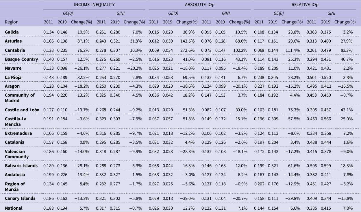
Table 2 shows the results of both income inequality and IOp in the equivalised disposable income through two indices, the Gini and the GE (0). We use the Gini index due to its easy interpretation and because it is widely used to measure inequality. Generalised Entropy GE (0) is also computed since this is the only measure with a path-independent decomposition (Foster and Shneyerov, Reference Foster and Shneyerov2000) using the arithmetic mean as reference and can be easily used to compute the contribution of the circumstances to IOp.
Estimates of inequality

According to the obtained results, North-western regions (Galicia, Asturias, Cantabria and Basque Country) and also two central regions (Madrid and La Rioja) experienced an increase in both income inequality and IOp whilst for the remaining regions we observe a decrease in both inequalities, with the exception of Castile and Leon and Castilla-La Mancha for which we observe an increase.
Likewise, in most regions we can see an increase in relative IOp. That is to say, the share of inequality of opportunity in overall inequality increases; and consequently, factors that are beyond individuals’ responsibility become more important in shaping individuals´ well-being and performance.
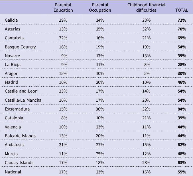
To answer our question ‘to what extent are family background characteristics important in shaping inequalities?’, once we get the estimates of IOp we estimate the contribution of the circumstances and pay attention to the amount of IOp due to Parental Education and Parental Occupation. To this end, we decompose IOp using the Shapley value procedure (Shorrocks, Reference Shorrocks2013), and we compute the marginal effects each variable has in IOp in terms of the GE (0) index.
Table 3 shows the average contribution of family background characteristics to IOp, these circumstances are of great relevance in shaping inequalities, the three of them account for about half or more of the total IOp. The exceptions are four regions of the northeast (Navarre, La Rioja, Aragon and Catalonia) where the relative importance of family background characteristics is lower.
Average contribution of family background circumstances

As it can be seen in this Section, both inequalities, income inequality and inequality of opportunity, both in levels and evolution, differ between regions. Additionally, the importance of family background characteristics to determine the levels of inequality of opportunity also varies greatly. For this reason, it is relevant to analyse the determinants of these regional differences.
Drivers of inequalities
The aim of this section is to know which are the main drivers of the observed inequalities across regions. We analyse the reasons behind the differences in inequality levels between regions and how these differences can be reduced.
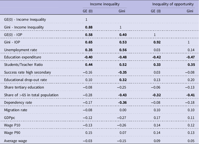
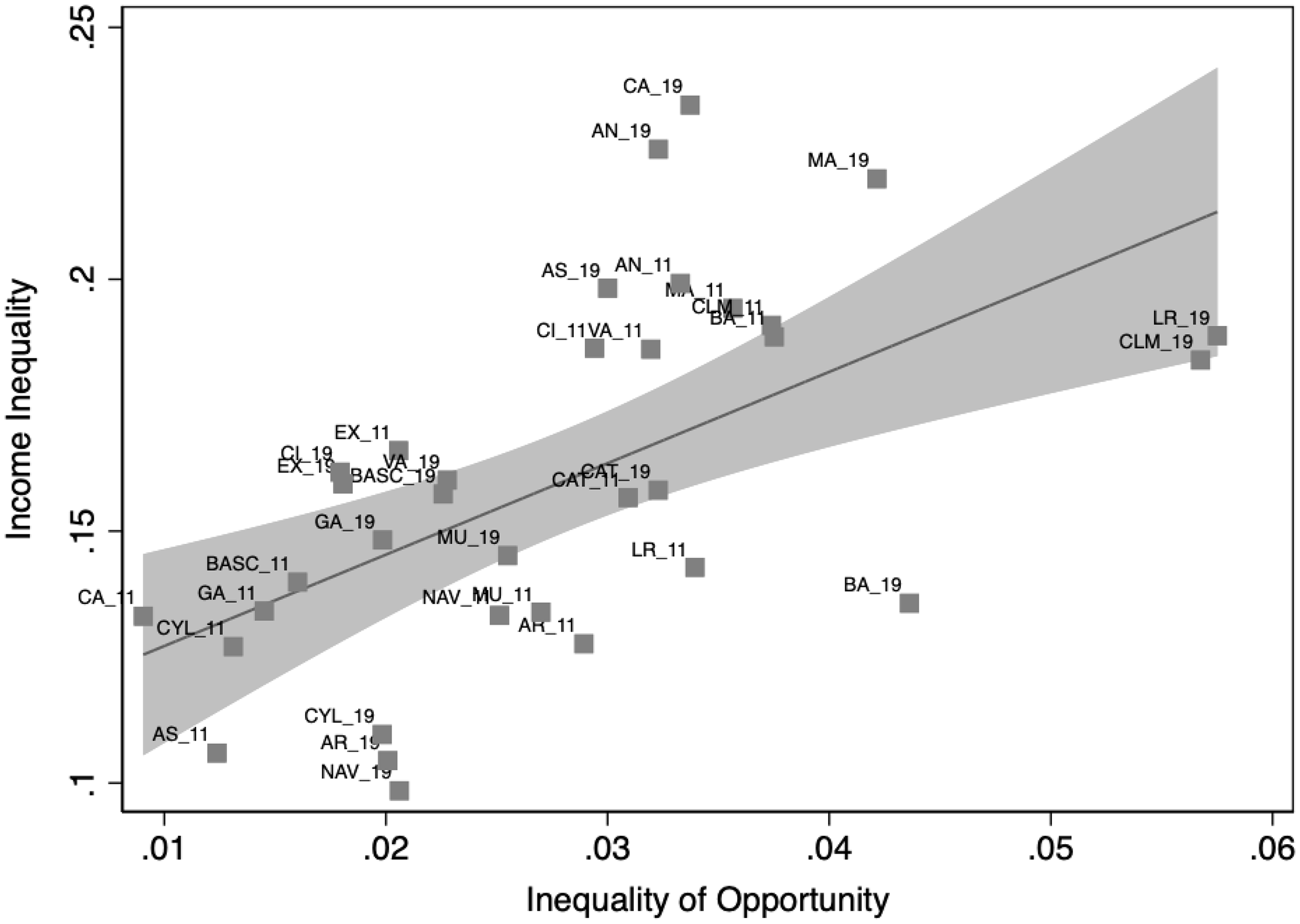
As a first step, we look at the association between inequality levels and several variables. We analyse the correlations between inequality variables and potential determinants of inequality, we include economic, demographic and educational variables. Table 4 shows the pairwise correlations, it can be seen that, as expected both sorts of inequality are positively and strongly correlated, as Figure 1 also illustrates.
Pairwise correlations

Significant correlations are in bold
Relationship between Income inequality and inequality of opportunity.

Regarding the economic variables included, income inequality is positively and significantly correlated with the unemployment rate, therefore, those regions with higher rates of unemployment also suffer from higher levels of income inequality. Nevertheless, its effect on IOp is not significant. The other economic variables included are the per capita Gross Domestic Product (GDP), the average wage, the wage of the tenth percentile and the wage of the ninetieth percentile. The GDPpc, the average wage and the wage of the 10th percentile are negatively correlated with income inequality and positively correlated with IOp, whilst the wage of the ninetieth percentiles is positively correlated with both sorts of inequalities. Nonetheless, these correlations are weak and non-significant.
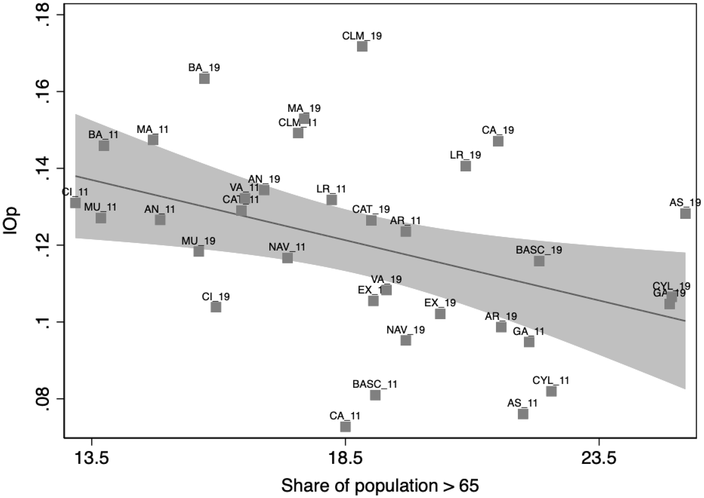
With regard to demographic variables, we include the share of population over sixty five years and the dependency rate, both variables are negatively correlated with the levels of inequality. Moreover, the correlation between the population shares over sixty five years and the inequality variables is quite strong and significant, as can be also seen in Figure 2. It implies that regions with aged population have less inequalities, possibly because retirement benefits an equalising effect on income. We also include the net inter-regional migration rate but its correlation with inequality is weak and not significant.
Relationship between IOp and the share of population over 65 years.
Educational variables seem to have the highest levels of correlation with inequality variables. As educational variables, we include five variables at regional level. The first of them is the share of individuals with tertiary education, which is negatively correlated with both income inequality and IOp, although this correlation is not significant. Then, the educational drop-out rateFootnote 2, which is positively and significantly correlated with income inequality and the success rate of high-secondary school which is negatively and significantly correlated with income inequality.
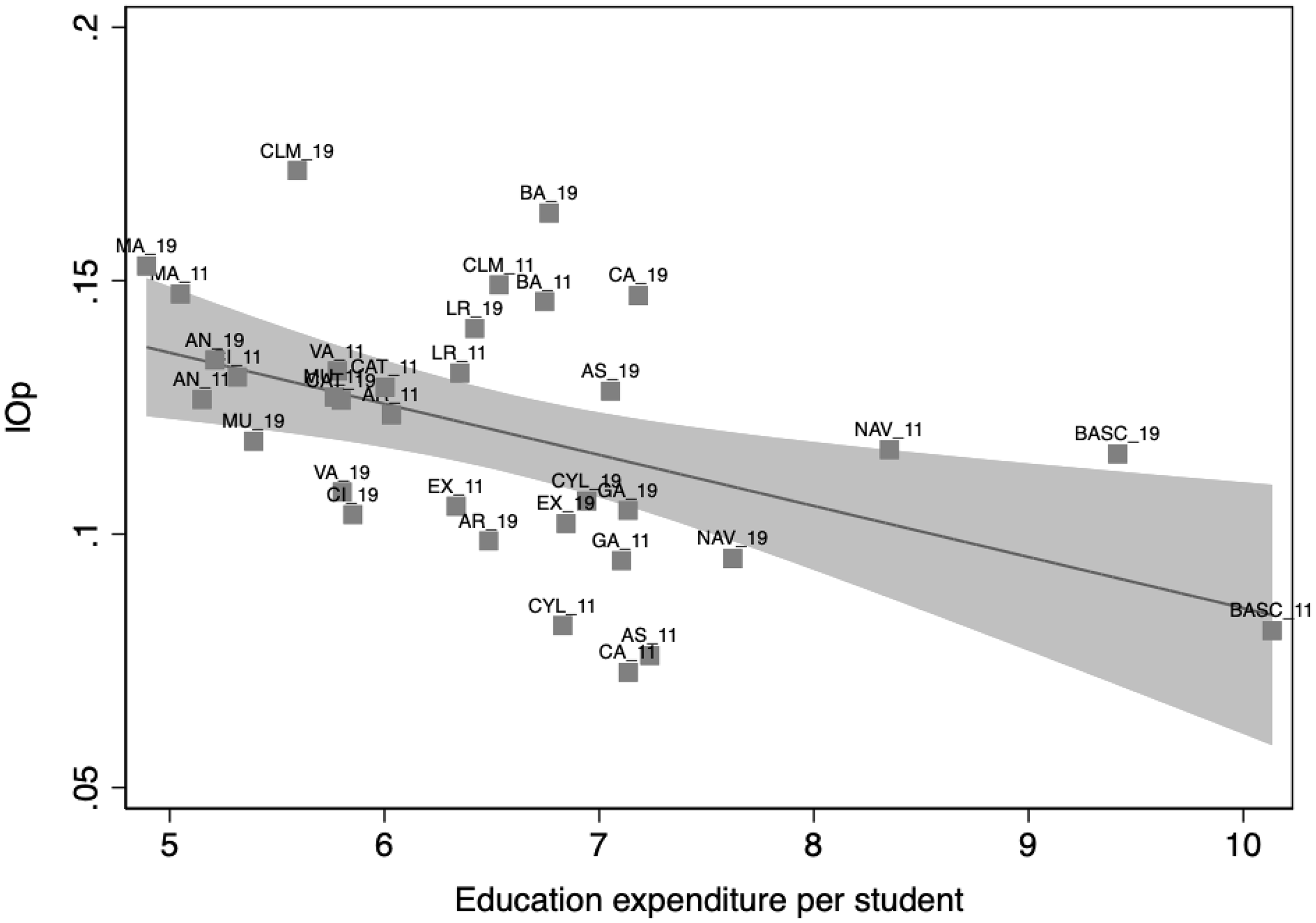
The two educational variables that show the highest level of correlation with the inequality variables are the average student/teacher ratio and the education expenditure per studentFootnote 3. The students/teacher ratio correlation implies that the higher the average number of students per teacher, the higher the levels of inequality and IOp. Additionally, the correlation between the education expenditure per student and the inequality variables shows that the greater the education expenditure the lower the inequality levels, this relationship is also illustrated by Figure 3. These results show that there is a significant association between the levels of inequality and educational resource endowments, both economic (educational expenditure) and human capital (students/teacher ratio). It is observed that those regions with a greater endowment of educational resource exhibit lower levels of inequality.
Relationship between IOp and the Education expenditure per student.
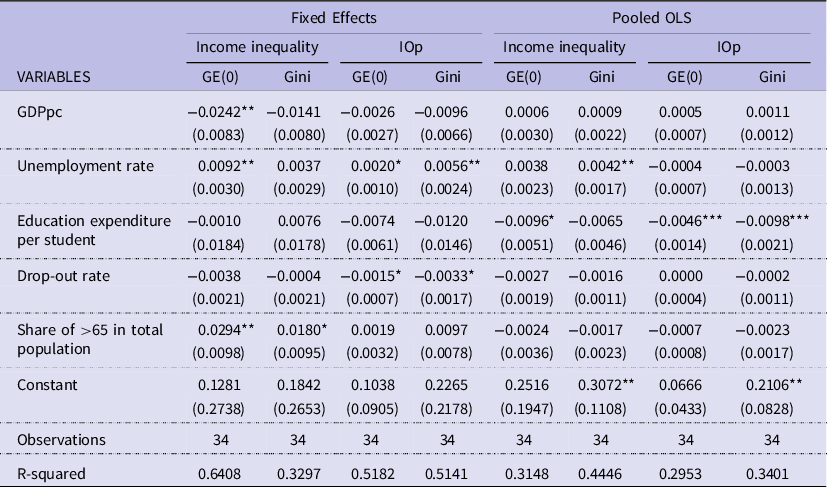
In addition to the pairwise correlations, we perform several regressions to see if the previously observed associations also entail causal relationships. Table 5 shows the results of the regressions – as expected not all positive and significant pairwise correlations are significant in the regression analysis. Moreover, regression results are not robust when comparing fixed effects and pooled Ordinary Least Squares (OLS).
Regressions’ results

Standard errors in parentheses.
***p < 0.01, **p < 0.05, *p < 0.1.
Still, the regression analysis shows that an increase in unemployment rate would cause an increase in the levels of income inequality. Additionally, the expenditure on education is significant to explain IOp, showing that an increase in education expenditure would reduce inequality of opportunity.
Summarising, the analysis carried out in this Section highlights the great relevance of education in reducing inequalities, especially the expenditure on education and the number of teachers.
Conclusions
Throughout this article we show the relevance of family background characteristics in shaping individuals’ income and the determinants of regional differences in levels of both income inequality and inequality of opportunity.
We wonder if familiar background characteristics have an impact on individuals’ disposable income. To test that, we compute inequality and IOp indices for the different regions. Our analysis reveals that family background has a great impact on individuals’ income and it is a crucial source of unequal opportunities.
Moreover, this analysis reveals that, for the Spanish regions, familiar background characteristics – in particular, parental education, parental occupation, and the financial situation during childhood – are of great importance in shaping individuals’ performance and opportunities of achieving a certain level of income.
Additionally, we analyse the main drivers of the regional differences in income inequality and IOp, finding that educational variables are highly associated to inequality levels. Moreover, the regression analysis shows that there is a causal relation between educational resource endowments and both income inequality and IOp – the analysis shows that regions that invest more in education experienced lower levels of inequality.
The obtained results suggest that different regional education policies, reflected in differences in expenditure per student, are an important determinant of regional inequalities, especially of inequalities of opportunity, which are the sort of inequalities beyond individuals’ responsibilities and therefore, considered unfair. Consequently, some policy implications can be drawn from this empirical evidence.
The results seem to indicate that an increase in social expenditures could have an equalising effect on income. In this sense, it is important to mention the work from Quiñonez (Reference Quiñonez2022), who found that in the case of Latin America social spending increases are associated with reduced levels of income inequality. He distinguishes four areas of social expending (social protection, education, health, and housing and community services) and shows that each of them has different effects on income inequality. Additionally, Ellison and Fenger (Reference Ellison and Fenger2013) show that the implementation of socially equitable and effective state policies or interventions depends on a thorough prior analysis of the relationship between labour market structures, inequality, social investment, and social protection in specific contexts.
This underlines the importance of specific policies that can directly and effectively address existing inequalities and specifically target the groups that need them. It is important when designing public policies to carry out analyses that clearly identify those individuals or groups susceptible to being targeted by the policies.
The analysis carried out in this article has allowed us to determine which are the most vulnerable groups and which are more likely to receive lower income and be, therefore, in a position of material disadvantage. These are individuals from disadvantaged family backgrounds, with parents who have a low level of education and who work in low-skilled occupations.
Therefore, it would be advisable to implement public policies targeting this vulnerable group. Additionally, given that this research shows that the greater the educational resource endowments (both human and material) the lower the levels of income inequality, it would be advisable to combine specific policies for vulnerable groups with policies aimed to increase educational resources. More specifically, redistributive policies could be combined with policies aimed at improving the quality of education and guaranteeing access to education regardless of socioeconomic factors and family background.
To sum up, policies aimed at ‘levelling the playing field’ seem to be necessary in order to improve the situation of those individuals who suffer a lack of opportunities in both educational and economic dimensions and who are more vulnerable to economic shocks.
Data availability statement
The data that support the findings of this study are available from the corresponding authors upon reasonable request.
Acknowledgements
We would like to thank the Editor and Reviewers for taking the time and effort to review the manuscript. We sincerely appreciate their valuable comments.
Disclosure statement
There are no competing interests to declare. Authors do not have any financial or non-financial competing interests to report.
Regressions’ results 2011
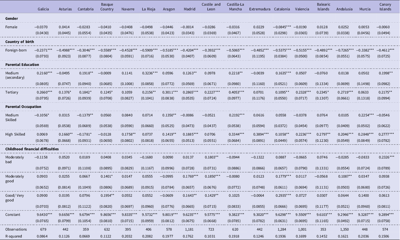
Standard errors in parentheses.
***p < 0.01, **p < 0.05, *p < 0.1.
Regressions’ results 2019
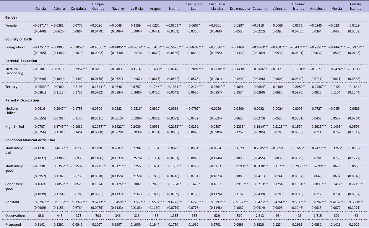
Standard errors in parentheses.
***p < 0.01, **p < 0.05, *p < 0.1.
Contribution of circumstances to inequality of opportunity in 2011 and 2019


 Open access