


Non-technical Summary
In paleobiology, continuous morphological traits—like limb lengths or skull dimensions—hold rich evolutionary information. However, these traits are often converted into discrete categories due to software limitations and difficulties handling missing data. This study presents a new implementation of the Brownian motion model in the widely used software MrBayes that allows direct analysis of continuous traits, even with substantial missing data. Simulations and analyses of pterosaur and ancient human datasets show that continuous traits, when used directly, can improve phylogenetic resolution compared with discretized versions. This work expands the analytical tool kit available for morphological and total-evidence phylogenetics in paleobiological research.
Introduction
Morphological traits are the primary or sole source of information for inferring the phylogenies of fossil taxa (Wiens Reference Wiens2004; Lee and Palci Reference Lee and Palci2015). For decades, maximum parsimony has been the dominant method in the field (Farris Reference Farris1970; Fitch Reference Fitch1971). In recent years, Bayesian inference, which better integrates various sources of information and accounts for uncertainties, has been emerging due to its desirable statistical properties (Ronquist and Huelsenbeck Reference Ronquist and Huelsenbeck2003). It not only infers tree topologies but also branch lengths in the unit of evolutionary distance. When combined with fossil ages, total-evidence or tip-dating approaches infer timetrees in geological units, evolutionary rates, and diversification patterns coherently (Pyron Reference Pyron2011; Ronquist et al. Reference Ronquist, Klopfstein, Vilhelmsen, Schulmeister, Murray and Rasnitsyn2012a; Zhang et al. Reference Zhang, Stadler, Klopfstein, Heath and Ronquist2016; Donoghue and Yang Reference Donoghue and Yang2016; Gavryushkina and Zhang Reference Gavryushkina, Zhang and Ho2020).
Discrete characters are the main type of data for applying these methods. Even though a substantial number of continuous traits are available, they have typically been discretized in morphological phylogenetics due to lack of feasible computational tools. In the parsimony school, Goloboff et al. (Reference Goloboff, Mattoni and Quinteros2006) added support for continuous traits by treating them as additive characters (Farris Reference Farris1970) in TNT (Goloboff and Catalano Reference Goloboff and Catalano2016). Statistical models for continuous traits have also been developed for decades. Trait evolution is typically modeled using a Brownian motion (BM) process (Felsenstein Reference Felsenstein1973, Reference Felsenstein1985; Freckleton Reference Freckleton2012) or an Ornstein–Uhlenbeck (OU) process (Felsenstein Reference Felsenstein1988; Hansen Reference Hansen1997; Butler and King Reference Butler and King2004). However, practical implementations for phylogenetic inference are sparse.
In the general form of the BM model, the variance–covariance matrix, R, has p(p − 1)/2 parameters describing the correlation among p continuous traits (Freckleton Reference Freckleton2012), making the computation either too expensive or unidentifiable, even when p is moderate. This involves more parameters when considering diffusion rate variation along the tree. Pre-estimating R seems a practical solution (Álvarez-Carretero et al. Reference Álvarez-Carretero, Goswami, Yang and dos Reis2019). When there are no missing or inapplicable states in the data, the implementation in MCMCTree focuses on estimating divergence times (Álvarez-Carretero et al. Reference Álvarez-Carretero, Goswami, Yang and dos Reis2019), while that in BEAST 2 (Zhang et al. Reference Zhang, Drummond and Mendes2023) can co-estimate tree topology and the times. In phylogenetic comparative methods, several R packages have been developed to study the traits of interest, assuming the phylogenies are known a priori (Pennell et al. Reference Pennell, Eastman, Slater, Brown, Uyeda, FitzJohn, Alfaro and Harmon2014; Revell Reference Revell2024).
However, empirical datasets typically contain many missing states. Deleting missing cells would result in a great loss of information. The ability to robustly handle missing data is not merely a “nice-to-have” feature, but an absolute “must-have” prerequisite. Apparently, handling missing data imposes great challenges. Even if R is known, state-of-the-art methods require either data augmentation or analytical integration (Mitov et al. Reference Mitov, Bartoszek, Asimomitis and Stadler2020; Hassler et al. Reference Hassler, Tolkoff, Allen, Ho, Lemey and Suchard2022), thus hindering their use in inferring phylogenies with moderate to large datasets with a high proportion of missing states. When the traits are assumed to be independent, RevBayes (Höhna et al. Reference Höhna, Landis, Heath, Boussau, Lartillot, Moore, Huelsenbeck and Ronquist2016) can handle continuous traits with missing data (Wynd et al. Reference Wynd, Khakurel, Kammerer, Wagner and Wright2025), but the implementation details have not been documented. According to our experience, complex models in RevBayes (especially those not covered in tutorials) can be difficult to set up and are not always reliable.
In this study, we move one step forward and implement the BM model for continuous traits in the widely used software MrBayes (Ronquist et al. Reference Ronquist, Teslenko, van der Mark, Ayres, Darling, Höhna, Larget, Liu, Suchard and Huelsenbeck2012b) for Bayesian phylogenetic inference. For simplicity, we do not currently consider correlation among traits. This allows us to incorporate any proportion of missing data and enables efficient likelihood calculation. The implementation can account for evolutionary rate variation across characters, among data partitions, and along the tree branches.
We first describe the implementation of the BM model. Then we perform computer simulations to briefly verify its correctness. Finally, we demonstrate its utility using two empirical datasets, pterosaurs and ancient humans, both of which have combined continuous and discrete characters.
Methods
We first assume the phylogeny is rooted and binary, with topology τ and branch lengths t = {ti} (i = 1, …, 2s − 2). The morphological traits are assumed to have evolved independently along the phylogeny following a BM process with diffusion rates r = {σ i 2} (i = 1, …, 2s − 2). We later show that the root position does not affect the likelihood.
The Likelihood
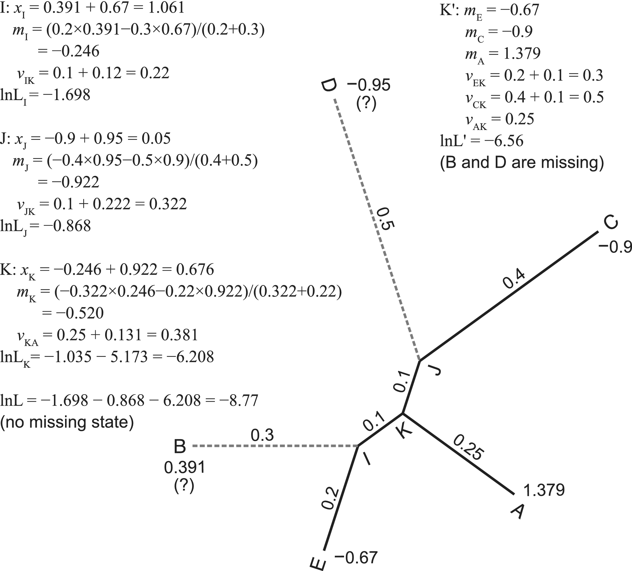
Let M be a matrix of p continuous traits for s species. The general formula of the likelihood function, f (M | τ, t, r), involves multivariate normal distributions (Felsenstein Reference Felsenstein1973; Freckleton Reference Freckleton2012). To avoid extensive computation, Felsenstein (Reference Felsenstein1973) introduced a pruning algorithm that computes independent contrasts while traversing the tree in post-order. He further eliminated the calculation of the root branch, resulting in the restricted maximum likelihood (REML; Felsenstein Reference Felsenstein1981). This is used in our implementation. A working example is shown in Figure 1.
Pruning algorithm without and with missing states. One continuous trait with state values at the tips of a five-taxa tree is used for illustration. We assume the root is at the branch leading to taxon A. The algorithm traverses the tree (internal nodes) in post-order, that is, I, J, K, and the root. For internal node k with two descendant nodes i and j, we calculate the contrast (xk = mi − mj), ancestral state (mk), and transformed branch length (vk). The contrasts follow independent normal distributions. According to the pulley principle, the root position does not affect the likelihood and can be placed anywhere in the tree. When the states at taxa B and D are missing, we simply prune the branches leading to them, resulting in a star tree with three tips, A, C, and E. Refer to the pseudocode in the Appendix for a more rigorous calculation.

Pulley Principle
Although the pruning algorithm was demonstrated on a rooted tree, Felsenstein (Reference Felsenstein1981) pointed out that the position of the root does not affect the likelihood. In fact, the root (“pulley”) can be “rolled onto any branch” of the tree. Thus, we can only infer an unrooted tree without further assumptions (such as a clock model or an out-group).
Missing States
We take advantage of the assumption of trait independence, and for each trait with missing states, we simply prune the branches leading to those states (illustrated in Fig. 1). The operation is trait-wise and can be performed during the application of the pruning algorithm (see the pseudocode in the Appendix). It results in a simple and efficient calculation that can handle any proportion of missing data. According to our knowledge, RevBayes handles continuous traits with missing data in a similar way (S. Höhna personal communication 2021).
Specifically, we use mk to denote the trait state at node k, and bk (σ k 2tk) for its branch length. If k is a tip, let
 $$ {v}_k=\left\{\begin{array}{c}0\hskip1.4em \mathrm{if}\;{m}_k\ \mathrm{is}\ \mathrm{NA},\\ {}{b}_k\hskip0.7em \mathrm{otherwise}.\end{array}\right. $$
If k is an internal node with two descendant nodes i and j, let
 $$ {v}_k=\left\{\begin{array}{c}0\hskip8.759999em \mathrm{if}\ \mathrm{both}\;{m}_i\hskip0.42em \mathrm{and}\hskip0.42em {m}_j\hskip0.42em \mathrm{are}\hskip0.42em \mathrm{NA},\\ {}{b}_k+{v}_i\hskip5em \mathrm{else}\ \mathrm{if}\;{m}_j\hskip0.42em \mathrm{is}\hskip0.42em \mathrm{NA},\\ {}{b}_k+{v}_j\hskip5em \mathrm{else}\ \mathrm{if}\;{m}_i\hskip0.42em \mathrm{is}\hskip0.42em \mathrm{NA},\\ {}{b}_k+\frac{v_i{v}_j}{v_i+{v}_j}\hskip2em \mathrm{otherwise};\end{array}\right. $$
 $$ {m}_k=\left\{\begin{array}{c}\mathrm{NA}\hskip4.4em \mathrm{if}\ \mathrm{both}\hskip0.42em {m}_i\hskip0.42em \mathrm{and}\hskip0.42em {m}_j\hskip0.42em \mathrm{are}\hskip0.42em \mathrm{NA},\\ {}{m}_i\hskip8.9em \mathrm{else}\ \mathrm{if}\hskip0.42em {m}_j\hskip0.42em \mathrm{is}\hskip0.42em \mathrm{NA},\\ {}{m}_j\hskip8.82em \mathrm{else}\ \mathrm{if}\hskip0.42em {m}_i\hskip0.42em \mathrm{is}\hskip0.42em \mathrm{NA},\\ {}\frac{m_i{v}_j+{m}_j{v}_i}{v_i+{v}_j}\hskip2.48em \mathrm{otherwise}.\end{array}\right. $$
The log-likelihood is a sum over all internal nodes whose child states are both available.
 $$ lnL=\sum \left[-\frac{1}{2}\ln \left(2\pi \right)-\frac{1}{2}\ln \left({v}_i+{v}_j\right)-\frac{{\left({m}_i-{m}_j\right)}^2}{2\left({v}_i+{v}_j\right)}\right]. $$
Practices
We highlight a few practices that are important in empirical inferences. They are supported in MrBayes.
First, times and diffusion rates are indistinguishable in non-clock analyses. The tree is unrooted, and the branch lengths are measured by “distance” (i.e., bi = tiσ i 2; i = 1, …, 2s − 3). The times and rates become identifiable in dating analyses with additional time information (either directly from the fossils [tip dating] or from node calibrations [node dating], or both) and clock model assumptions. The inferred timetree is rooted, and the clock rates are the diffusion rates (r = {σ i 2}; i = 1, …, 2s − 2). Diffusion rate variation along branches is supported by relaxed clock models (e.g., Thorne and Kishino Reference Thorne and Kishino2002; Drummond et al. Reference Drummond, Ho, Phillips and Rambaut2006; Lepage et al. Reference Lepage, Bryant, Philippe and Lartillot2007).
Evolutionary rate variation among data partitions typically should be considered. This feature is supported by a uniform Dirichlet distribution for the relative partition rates (Zhang et al. Reference Zhang, Stadler, Klopfstein, Heath and Ronquist2016). Diffusion rate variation among characters is also supported by averaging a discretized gamma (Yang Reference Yang1994) or lognormal distribution (Wagner Reference Wagner2012; Harrison and Larsson Reference Harrison and Larsson2015). However, it is more practical to normalize or standardize the continuous traits, so considering character-rate variation would be unnecessary. Our implementation supports both normalized and standardized data.
Normalization has been considered a critical step in the parsimony implementation (Goloboff et al. Reference Goloboff, Mattoni and Quinteros2006; Mongiardino Koch et al. Reference Mongiardino Koch, Soto and Ramírez2015). It rescales all the trait values to be between 0 and 1, that is, mk′ = (mk − m min) / (m max − m min + ε), where m max and m min are the maximum and minimum observed values of the trait, and ε is a very small number (e.g., 0.0001). Relative to this, discretizing a trait into n states is simply taking the integer part of nmk′ (Thiele Reference Thiele1993). Alternatively, standardization is a common technique in statistical analyses that brings different traits to the same scale. It subtracts mk by the sample mean and then divides by the standard deviation. For a trait with skewed values, it appears reasonable to log-transform the values before normalizing or standardizing them, to approximately conform them to normality and potentially improve model fit.
Simulation
We performed computer simulations to verify our implementation. We first generated variable timetrees from a birth–death process using TreeSim (Stadler Reference Stadler2011) in R (R Core Team 2021) with a birth rate of 5.0 and a death rate of 4.0, conditioned on a root age of 1.0. The ages are on a relative scale and can be arbitrarily rescaled depending on the chosen time unit. We kept 100 trees with no more than 50 tips to make sure the data size is manageable.
For each tree, we simulated the evolution of continuous traits under a BM process with a diffusion rate of 1.0. Each trait is an independent draw from the same BM process. The starting state at the root was set to 0.0. We recorded a moderate number of 200 continuous traits in the data matrix. In addition to the complete data, we also generated datasets with 50% missing states in the extinct taxa and 10% missing in the extant taxa, mimicking observations in empirical datasets. Specifically, we replaced each state by a question mark with the corresponding probability.
For comparisons, we also generated 200 variable binary discrete characters under the Mkv model (Lewis Reference Lewis2001). The substitution rate was set to 1.0 (strict clock; Zuckerkandl and Pauling Reference Zuckerkandl, Pauling, Bryson and Vogel1965). And to test the functionality of supporting mixed data types, we generated data matrices each containing 100 continuous and 100 discrete characters.
We performed both non-clock and tip-dating analyses for each dataset using MrBayes (Ronquist et al. Reference Ronquist, Teslenko, van der Mark, Ayres, Darling, Höhna, Larget, Liu, Suchard and Huelsenbeck2012b). In the non-clock analyses, we used uniform prior for the tree topologies and gamma-Dirichlet prior for the branch lengths (Zhang et al. Reference Zhang, Rannala and Yang2012). The inferred trees are unrooted. In the tip-dating analyses, we used the constant-rate fossilized birth–death prior (Stadler Reference Stadler2010; Heath et al. Reference Heath, Huelsenbeck and Stadler2014) for the timetrees and strict clock model for the evolutionary rates. The tip ages were assigned their true values assuming they are perfectly known. The inferred trees are rooted due to the clock assumption. For each inference, two independent chains were executed for enough generations to ensure convergence and sufficient effective sample sizes (ESS > 100). The posterior tree samples were summarized as a 50% majority-rule consensus tree.
We employed the Quartet metric (Estabrook et al. Reference Estabrook, McMorris and Meacham1985) to compare the inferred tree topology with the true one that generated the data. It has several advantages over the traditional Robinson-Foulds metric (Robinson and Foulds Reference Robinson and Foulds1981). Additionally, we calculated the Strict Joint Assertion (which is the number of quartets that are resolved identically in both trees over that resolved either identically or differently in both trees; Estabrook et al. Reference Estabrook, McMorris and Meacham1985) as a measure of accuracy, and the percentage of resolved internal branches (the number of internal branches in the estimated consensus tree over that in the true tree) as precision.
To investigate the branch length estimates, we fixed the tree topology to the one used to simulate the data in another round of inference. The branch lengths in the tip-dating analyses are directly comparable; while in the non-clock analyses, the true tree was unrooted for comparison (by joining the two branches connecting the root). We calculated the root-mean-square error to assess the accuracy with which the branch lengths were estimated, and the mean widths of 95% credibility intervals as precision.
Simulation scripts and MrBayes commands can be found in Supplementary Material. Because RevBayes also supports phylogenetic inference using continuous traits under the BM model, as a brief verification, we also included a test comparing the non-clock inference results between MrBayes and RevBayes using a continuous trait matrix of 10 taxa generated in the simulation.
Empirical Data
We applied the new implementation to datasets of pterosaurs (Andres Reference Andres2021) and ancient humans (Ni et al. Reference Ni, Ji, Wu, Shao, Ji, Zhang and Liang2021); each contains both continuous and discrete characters.
Pterosaurs
The pterosaur dataset has 52 continuous traits and 223 discrete ones for 177 species (Andres Reference Andres2021). However, we excluded 65 of them that have more than 70% missing states in both data types, as well as one out-group species with a highly uncertain age, resulting in 111 species (three of them are treated as an out-group). The original traits are unscaled measurements, thus we normalized them to be within the range of 0 and 1. For comparison, we also discretized the continuous traits into six ordered states, which was the usual treatment before the availability of the BM model.
The continuous and discrete characters are naturally divided as two partitions. Rate variation between the partitions was accounted for using a uniform Dirichlet distribution. In the tip-dating analyses, fossil ages are gathered from the Paleobiology Database. As MrBayes does not fully support analyzing purely fossil taxa, each fossil age was reduced by 66, that is, treating the two youngest species as extant. The original data include 12 species that extend to 66 Ma, and considering potentially unsampled species, we set the sampling proportion of “extant” species to 0.1. The prior for the root age was assigned an offset-exponential distribution with mean 186 (the boundary between Permian and Triassic, minus 66) and offset 176 (close to the age of the oldest out-group fossil, Euparkeria capensis). We tested both the independent-lognormal (Drummond et al. Reference Drummond, Ho, Phillips and Rambaut2006) and autocorrelated-lognormal (Thorne and Kishino Reference Thorne and Kishino2002) relaxed clock models. In each case, we either linked or unlinked the clock rate variation for the two partitions.
We executed four independent runs and four Metropolis-coupled chains per run for 40 million generations in the non-clock analysis, or for 80 million generations in the tip-dating analyses, and sampled every 1000 generations. The beginning 25% samples were discarded as burn-in, and the remaining samples from the four runs were combined after confirming consistency. We checked the parameter traces, effective sample sizes, average standard deviation of split frequencies and treespaces using the R package RWTY (Warren et al. Reference Warren, Geneva and Lanfear2017).
Ancient Humans
The human dataset has 400 continuous traits and 234 discrete ones for 55 operational taxonomic units (Ni et al. Reference Ni, Ji, Wu, Shao, Ji, Zhang and Liang2021). The original study discretized the continuous traits into six ordered states. Here, we compare those results with analyses using continuous traits modeled under the BM process. The continuous traits have already been normalized.
We focused on the tip-dating analyses and used the white noise relaxed clock model (Lepage et al. Reference Lepage, Bryant, Philippe and Lartillot2007) to match the original study. We either linked or unlinked the clock rate variation for the two partitions. The root age prior was assigned Uniform(2.8, 3.6) (time is measured by million years). Homo habilis was used as the out-group, and we did not enforce extra topological constraints to see if the BM model could improve resolution of the resulting tree. We executed four independent runs and four Metropolis-coupled chains per run for 50 million generations and sampled every 500 generations.
Data, commands, and results (consensus trees in Newick format) can be found in the Supplementary Material.
Results
Simulation
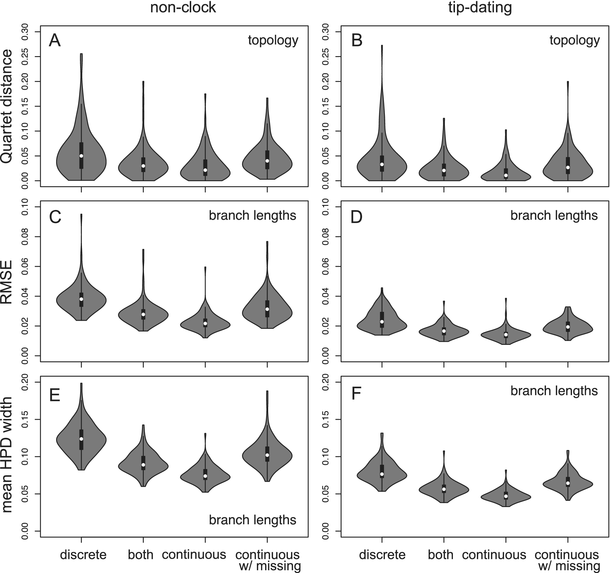
The tree topology is estimated more reliably using continuous traits than using discrete characters, as measured by the Quartet distances (Fig. 2). This results from both increased accuracy and precision (Supplementary Fig. S1). The branch length estimation also has higher accuracy and precision (less bias and narrower credibility interval; Fig. 2). Similarly, using mixed data is more beneficial than using discrete characters alone (with an equal number of characters). Having missing data (50% in fossil taxa) reduces the accuracy and precision, resulting in similar performance to that using discrete data without missing states (Fig. 2).
Quartet distance metric comparing the inferred tree topology with the true tree (A and B), and root-mean-square error (RMSE; C and D) and mean widths of 95% highest posterior density (HPD) intervals (E and F) of the estimated branch lengths. Each violin plot contains 100 replicates. The four data types are: (1) 200 variable binary discrete characters; (2) 100 variable binary discrete characters and 100 continuous traits; (3) 200 continuous traits; and (4) 200 continuous traits with 50% missing states in the extinct taxa and 10% missing in the extant taxa.

The branch lengths are more accurately and precisely estimated in the tip-dating analyses; this is due to the use of tip dates, which increases the information in the data, and of simple strict clock assumption, which just introduces one extra parameter. Overall, the simulation results indicate that the relevant functionalities are correctly implemented.
Pterosaurs
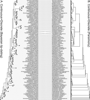
The inferred trees have good resolution in all the analyses performed after removing the species with more than 70% missing states (Supplementary Material, tree files). The inferred topologies generally agree with the most parsimonious tree (Fig. 3). The average substitution rate of the discrete data partition is about four times the diffusion rate of the continuous data partition (Supplementary Material, log files).
Tanglegram comparing the 50% majority-rule consensus tree from the Bayesian tip-dating analysis (A) to the strict consensus of the most parsimonious trees from TNT (B) using both continuous (normalized) and discrete morphological characters of pterosaurs. The relaxed clock model is independent-lognormal shared between the two partitions in the tip-dating analysis.

For the tip-dating analyses, convergence and mixing are good under the independent-lognormal relaxed clock model with either shared or unlinked rates between the two partitions. However, given the limited number of characters, particularly continuous ones, unlinking the clock rates does not appear beneficial for timetree inference, especially considering it doubles the number of parameters. Convergence and mixing are significantly more difficult under the autocorrelated-lognormal relaxed clock model, especially when the clock rates are unlinked (Supplementary Material, log files). We have to rerun the analyses multiple times to achieve convergence of all the chains. The marginal likelihood under the autocorrelated-lognormal model is much lower than that under the independent-lognormal model (roughly assessed by the harmonic mean estimates; Supplementary Material, log files). Therefore, we prefer the results obtained under the linked independent-lognormal relaxed clock model.
Ancient Humans
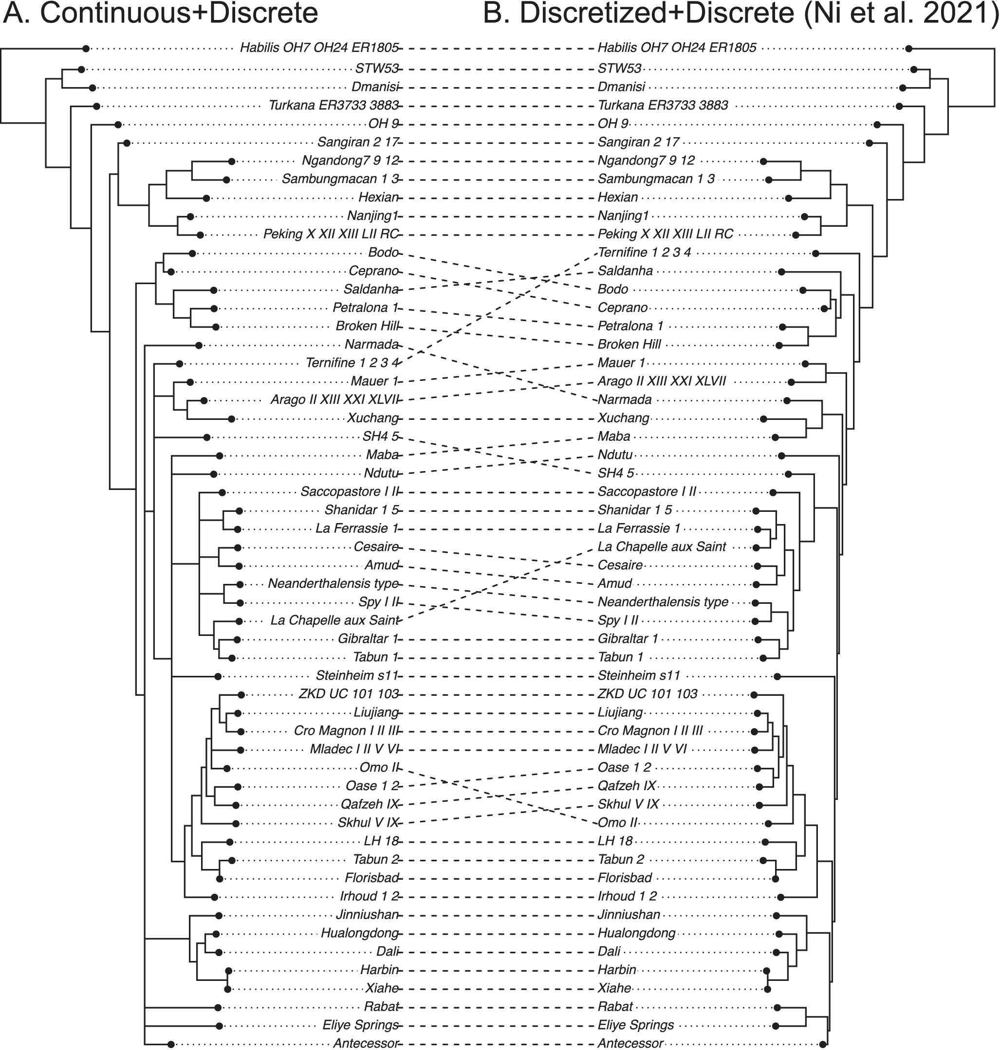
The dated phylogeny using both continuous and discrete characters shows improved resolution compared with that obtained when the continuous characters are discretized (Supplementary Material, tree files). Discretization appears to have caused a loss of information. The average substitution rate of the discrete data partition is about eight times the diffusion rate of the continuous data partition. Compared with the pterosaur dataset, this dataset includes many more continuous traits; as a result, we can infer different patterns of branch rate variation across partitions more reliably (Supplementary Material).
The original study enforced several topological constraints based on the most parsimonious tree (Ni et al. Reference Ni, Ji, Wu, Shao, Ji, Zhang and Liang2021). Without these constraints, the present results show unresolved relationships among some lineages (Fig. 4). Note that the most parsimonious tree only represents a point estimate without considering uncertainties. The treespace appears multimodal in the human data compared with the treespace in the pterosaur data (Supplementary Figs. S2, S3). Nevertheless, our aim is to just illustrate the usage of the BM model rather than to clarify human evolution, which is not possible based on this single dataset.
Tanglegram comparing the 50% majority-rule consensus tree using both continuous (normalized) and discrete morphological characters (A) with that using discretized continuous and discrete characters (B) of ancient humans. Both analyses used the white noise relaxed clock unlinked between the two partitions. The original study (tree on the right) enforced 10 topological constraints referring to the most parsimonious tree from TNT using both continuous and discrete characters (Ni et al. Reference Ni, Ji, Wu, Shao, Ji, Zhang and Liang2021).

Discussion
The ability to leverage continuous traits in phylogenetic inference is an appealing feature. Our study provides an efficient implementation of the BM model for Bayesian phylogenetic inference using continuous traits with missing states, integrated into the widely used software MrBayes. The implementation extends a suite of existing features toward morphological and total-evidence phylogenetics, combining continuous and discrete characters as well as molecular sequences.
Our simulation results indicate that continuous traits contain more phylogenetic information than discrete traits evolved at the same rate. Discrete characters could suffer from multiple hits, especially when the substitution rate is high; by contrast, continuous traits are less saturated. Similar patterns have been shown in a previous simulation study comparing continuous and discrete characters evolved at several different rates (Parins-Fukuchi Reference Parins-Fukuchi2018). Continuous traits should preferably be directly incorporated when available rather than discarded or discretized.
We implemented an approach that efficiently handles missing states by pruning branches. However, we still estimate the same number of branch lengths, as there were no missing data (e.g., 2s − 3 for unrooted tree). We do not expect a taxon with completely missing states or with states that do not overlap with those of other taxa, so there is information to infer each length. But the missing states in a real dataset are unlikely randomly distributed, thus the reliability of each branch length estimate is likely data dependent.
One limitation of our implementation is that correlation among traits is not considered. Simulation studies have shown that topological inference is relatively robust to violations of the trait-independence assumption (Parins-Fukuchi Reference Parins-Fukuchi2018), but evolutionary rates (or branch lengths in non-clock analyses) are largely overestimated (Álvarez-Carretero et al. Reference Álvarez-Carretero, Goswami, Yang and dos Reis2019). Thus, we advise performing subsequent comparative analyses that properly account for among-trait correlations to study the evolution of particular traits of interest.
Acknowledgments
This research was supported by the National Key Research and Development Program of China (2023YFF0804502 to C.Z.) and the National Natural Science Foundation of China (42172006 to C.Z.).
Author Contribution
C.Z. designed the study and led the analyses. Both authors contributed to the implementation in MrBayes. C.Z. led the interpretation of the results and writing of the manuscript. Both authors revised the manuscript and gave final approval for publication.
Competing Interests
The authors declare no competing interests.
Data Availability Statement
Electronic Supplementary Material is available from the Zenodo Digital Repository (https://doi.org/10.5281/zenodo.17647357). The Brownian model is implemented in a feature branch of MrBayes (https://github.com/zhangchicool/MrBayes) and will be merged to the main branch for the upcoming release (version 3.2.8).
Appendix
Pruning algorithm
1: Initialize log-likelihood: lnL ← 0
2: For each trait c:
3: For each node k in T (post-order):
4: If k is a tip node:
5: If m[c,k] is NA:
6: v[c,k] ← 0
7: Else:
8: v[c,k] ← b[k] // branch length of k in T
9: Else (k is an internal node):
10: Let i and j be the two child nodes of k
11: If m[c,i] and m[c,j] are both NA:
12: v[c,k] ← 0
13: m[c,k] ← NA
14: Else if m[c,i] is observed and m[c,j] is NA:
15: v[c,k] ← b[k] + v[c,i]
16: m[c,k] ← m[c,i]
17: Else if m[c,i] is NA and m[c,j] is observed:
18: v[c,k] ← b[k] + v[c,j]
19: m[c,k] ← m[c,j]
20: Else (both m[c,i] and m[c,j] are observed):
21: v[c,k] ← b[k] + v[c,i]*v[c,j] /(v[c,i]+v[c,j])
22: m[c,k] ← (v[c,j]*m[c,i] + v[c,i]*m[c,j])/(v[c,i]+v[c,j])
23: lnL ← lnL -0.5*log(2*pi) -0.5*log(v[c,i]+v[c,j])
-0.5*(m[c,i]-m[c,j])^2 /(v[c,i]+v[c,j])
24: Return lnL

 Open access