


1. Introduction
Turbulent dispersion and mixing of tracers, such as contaminants or greenhouse gases, is a ubiquitous phenomenon of interest in environmental and engineering applications. In many cases of interest, the scalar tracer is emitted continuously by a localised small (point-like) source, and the characteristic size of the source defines the initial size of the dispersing contaminant cloud. Turbulent eddies will interact with this dispersing plume and, depending on their characteristic size relative to the plume's instantaneous size, will be more effective in dispersing or transporting it across the turbulent flow. The overall dispersion process is then typically ascribed to two processes referred to as the relative dispersion and the meandering (e.g. Gifford Reference Gifford1959; Cassiani et al. Reference Cassiani, Bertagni, Marro and Salizzoni2020) of the plume. Under the effects of meandering and relative dispersion, the substance dispersing from a small localised source will, in general, display large fluctuations when the time evolution of the contaminant concentration is observed at a fixed point in space (e.g. Wilson Reference Wilson1995; Cassiani, Franzese & Albertson Reference Cassiani, Franzese and Albertson2009; Cassiani et al. Reference Cassiani, Bertagni, Marro and Salizzoni2020). The statistical characterisation of this fluctuating time series is typically obtained through the statistical moments,
 \begin{equation} \left\langle c^n(\boldsymbol{x}) \right\rangle = \frac{1}{\Delta t} \int_{0}^{\Delta t} c^n(\boldsymbol{x},t)\,{\rm d}t, \end{equation}
where  $c(\boldsymbol {x},t)$ is the scalar concentration at a specific point in space and time, and the integral extends over a time interval $\Delta t$. In many processes that are linearly related to the concentration levels of the dispersing substance, the knowledge of the first moment, i.e. the mean value, is sufficient to characterise it. However, several previous studies (e.g. ten Berge, Zwart & Appelman Reference ten Berge, Zwart and Appelman1986; Hilderman, Hrudey & Wilson Reference Hilderman, Hrudey and Wilson1999; Balkovsky & Shraiman Reference Balkovsky and Shraiman2002; Schauberger et al. Reference Schauberger, Piringer, Knauder and Petz2011) have shown that toxicity effects, flammability and odour nuisance are instead highly nonlinearly related to contaminants’ concentration fluctuations. In such cases, information about higher-order moments ( ${>}1$, i.e. other than the mean) of the scalar probability density function (p.d.f.) is required to correctly understand and model the dependent chemical, physical or biological processes. Recently, the role of concentration fluctuations has also been carefully considered in understanding the representativeness and interpretation of field observations of pollutants (Ražnjevic et al. Reference Ražnjevic, van Heerwaarden, van Stratum, Hensen, Velzeboer, van den Bulk and Krol2022b; Schulte et al. Reference Schulte, van Zanten, van Stratum and de Arellano2022) and in designing optimised pollutant plume sampling strategies (Ražnjevic, van Heerwaarden & Krol Reference Ražnjevic, van Heerwaarden and Krol2022a).
Given the large relevance in many applications, the dispersion of plumes has been the subject of many experimental and modelling investigations, as recently reviewed by Cassiani et al. (Reference Cassiani, Bertagni, Marro and Salizzoni2020). Many field studies in the atmospheric surface layer have been performed under varying stability conditions (e.g. Hanna Reference Hanna1984; Sawford, Frost & Allan Reference Sawford, Frost and Allan1985; Mylne & Mason Reference Mylne and Mason1991; Mylne Reference Mylne1992; Yee, Wilson & Zelt Reference Yee, Wilson and Zelt1993; Yee et al. Reference Yee, Chan, Kosteniuk, Chandler, Biltoft and Bowers1995; Mikkelsen et al. Reference Mikkelsen, Jørgensen, Nielsen and Ott2002; Munro, Chatwin & Mole Reference Munro, Chatwin and Mole2003; Finn et al. Reference Finn, Carter, Eckman, Rich, Gao and Liu2018, among others). However, among the various approaches that have advanced our understanding of plume dispersion and related concentration fluctuations, wind-tunnel laboratory studies under neutral stratification have played a prominent role. Starting with the early works of Robins (Reference Robins1978) and Netterville (Reference Netterville1979), to the fundamental study of Fackrell & Robins (Reference Fackrell and Robins1982) and the most recent contributions of Nironi et al. (Reference Nironi, Salizzoni, Marro, Mejean, Grosjean and Soulhac2015) and Talluru, Philip & Chauhan (Reference Talluru, Philip and Chauhan2018), these investigations have elucidated many aspects of the fluctuating behaviour of scalar plumes at approximately unitary Schmidt number, i.e. with molecular diffusivity ( $D$) and viscosity ( $\nu$) having similar values. Still, some aspects of the dispersing plume could not be fully captured due to the technical difficulties in implementing this type of laboratory measurement. For example, the early plume dispersion phases were generally neglected due to the perturbation induced by the emitting source. Similar to the laboratory studies mentioned above, numerical approaches using large-eddy simulation (LES) were employed with configurations resembling those of wind tunnels. In an early study by Sykes & Henn (Reference Sykes and Henn1992), due to the coarse grid resolution, near-source effects were simulated using a semi-empirical parametrised subgrid dispersion (Sykes, Lewellen & Parker Reference Sykes, Lewellen and Parker1984) that was tuned to match the laboratory experiment of Fackrell & Robins (Reference Fackrell and Robins1982). Xie et al. (Reference Xie, Hayden, Voke and Robins2004b, Reference Xie, Hayden, Robins and Voke2007) investigated dispersion and concentration fluctuations with finer spatial discretisation, but it was still insufficient to reproduce the near-field effects of varying source sizes. More recently, Ardeshiri et al. (Reference Ardeshiri, Cassiani, Park, Stohl, Stebel, Pisso and Dinger2020) addressed the grid requirements for using LES to accurately investigate the behaviour of the concentration field from small localised sources, showing that atmospheric LES provides a trustworthy representation of the concentration p.d.f. moments up to the fourth order for a dispersing plume, provided that the grid resolution is adequate. Here, we advance this previous study and use the same LES code and grid settings as Ardeshiri et al. (Reference Ardeshiri, Cassiani, Park, Stohl, Stebel, Pisso and Dinger2020) to comprehensively investigate the high-order statistics of concentration fluctuations, including the effects of varying source elevation and size. This study aims to complete previous wind-tunnel and numerical investigations by covering aspects that were previously not investigated. To our knowledge, our current dataset is unique due to the availability of the three-dimensional plume and both crosswind and vertical profiles, including the very early phases of dispersion, for source locations spanning from the ground to the middle of the boundary layer, and furthermore, for covering two different source sizes.
The methods used here in simulating the atmospheric turbulent flow and dispersion in a neutral boundary layer are briefly explained in § 2. In § 3 we analyse the main features of the turbulent velocity field, whose details were presented and discussed extensively in Ardeshiri et al. (Reference Ardeshiri, Cassiani, Park, Stohl, Stebel, Pisso and Dinger2020). Noteworthy, § 3 contains a novel analysis of the spectral distribution of energy in the most energetic scale of the velocity components, which is needed for the subsequent discussion of the energetic scales in the scalar tracer spectrum. Section 4 covers the scalar field with a focus on the fluctuations. The mean field characteristics are discussed in § 4.1 as a prerequisite for further analysis. The variance of the concentration fluctuations is discussed in detail in § 4.2, including a discussion of the evolution of the double-peak behaviour in the near-source dispersion for elevated plumes and its persistence for near-ground-level sources. Subsequently, in § 4.3 the focus is on the scalar power spectral density with a complete analysis of the most energetic scales of the scalar spectrum, in relation to recent findings (Talluru, Philip & Chauhan Reference Talluru, Philip and Chauhan2019). The analysis of the spectrum of elevated plumes is completed using a stochastic model and theoretical arguments, clarifying both the link between the location of the peak in the spectrum of the velocity components and that in the concentration spectrum, and the downwind evolution of the spectral peak in the concentration spectrum. For the ground-level sources, only a qualitative discussion of the evolution of the shape of energetic scales in the spectrum is possible. In § 4.4 the crosswind and along-wind evolution of the high-order scaled central moments intensity, skewness and kurtosis of the concentration p.d.f. is considered. The evolution of the higher moments is also linked to the expected shape of the concentration p.d.f., considering the limiting cases of the gamma and Gaussian p.d.f.s. The analysis also includes an investigation of an empirical relation (Fackrell & Robins Reference Fackrell and Robins1982) between the peak concentration and the concentration standard deviation. Finally, we investigate the intermittency of the concentration time series in § 4.5, highlighting its dependence on the threshold chosen in its definition. The summary and discussion are presented in § 5.
2. Methods
Numerical simulations are performed with the freely available LES open-source code PALM (Maronga et al. Reference Maronga, Gryschka, Heinze, Hoffmann, Kanani-Sühring, Keck, Ketelsen, Letzel, Sühring and Raasch2015). The LES dataset is archived and described in Appendix C. The model is set to solve the non-hydrostatic, filtered, incompressible Navier–Stokes equations in Boussinesq-approximated form in a half-channel flow. The half-channel flow, driven by a pressure gradient, has been adopted by several authors as an approximation of a boundary-layer flow (see Shaw & Schumman Reference Shaw and Schumman1992; Porté-Agel, Meneveau & Parlange Reference Porté-Agel, Meneveau and Parlange2000; Xie et al. Reference Xie, Voke, Hayden and Robins2004a,Reference Xie, Hayden, Voke and Robinsb; Bou-Zeid, Meneveau & Parlange Reference Bou-Zeid, Meneveau and Parlange2005; Cassiani, Katul & Albertson Reference Cassiani, Katul and Albertson2008; Huang, Cassiani & Albertson Reference Huang, Cassiani and Albertson2009; Stevens, Wilczek & Meneveau Reference Stevens, Wilczek and Meneveau2014; Margairaz et al. Reference Margairaz, Giometto, Parlange and Calaf2018, among others). The simulation evolves in time until reaching a steady state, at which the half-channel width can be interpreted as the boundary-layer depth (Porté-Agel et al. Reference Porté-Agel, Meneveau and Parlange2000). The flow dynamics develop at a formally infinite Reynolds number since molecular viscosity is neglected and the transfer of energy occurs only through a subgrid scale (SGS) model (e.g. Deardorff Reference Deardorff1970; Geurts & Frohlich Reference Geurts and Frohlich2002; Piomelli & Balars Reference Piomelli and Balars2002; Bou-Zeid et al. Reference Bou-Zeid, Meneveau and Parlange2005; Stevens et al. Reference Stevens, Wilczek and Meneveau2014; Ardeshiri et al. Reference Ardeshiri, Cassiani, Park, Stohl, Stebel, Pisso and Dinger2020). This implies that the advection–diffusion equation, for the transport of a passive scalar, is solved neglecting the molecular diffusivity and using SGS diffusivity for the scalar, linked to that for momentum via a subgrid Schmidt number (e.g. Moeng & Wyngaard Reference Moeng and Wyngaard1988; Maronga et al. Reference Maronga, Gryschka, Heinze, Hoffmann, Kanani-Sühring, Keck, Ketelsen, Letzel, Sühring and Raasch2015; Ardeshiri et al. Reference Ardeshiri, Cassiani, Park, Stohl, Stebel, Pisso and Dinger2020). A rough-wall model is used to ensure the correct momentum transfer at the solid boundary (e.g. Deardorff Reference Deardorff1970; Moeng Reference Moeng1984; Andren et al. Reference Andren, Brown, Mason, Graf, Schumann, Moeng and Nieuwstadt1994; Pope Reference Pope2000; Brasseur & Wei Reference Brasseur and Wei2010).
As discussed in detail in Maronga et al. (Reference Maronga, Gryschka, Heinze, Hoffmann, Kanani-Sühring, Keck, Ketelsen, Letzel, Sühring and Raasch2015) and Ardeshiri et al. (Reference Ardeshiri, Cassiani, Park, Stohl, Stebel, Pisso and Dinger2020), the PALM modelling framework allows for a selection of numerical schemes and closures. Here we use the same setting validated in Ardeshiri et al. (Reference Ardeshiri, Cassiani, Park, Stohl, Stebel, Pisso and Dinger2020), to which the reader is referred for an exhaustive description. The advection terms in the prognostic LES equations are discretised using the Piacsek & Williams (Reference Piacsek and Williams1970) second-order, energy-conserving numerical scheme. For the scalar plume dispersion, the monotone locally modified version of Bott's advection scheme proposed by Chlond (Reference Chlond1994) is used.
The size of the computational domain is  $4.8\ {\rm m} \times 0.8\ {\rm m} \times 0.8\ {\rm m}$ in along-wind ( $x$), crosswind ( $y$) and vertical ( $z$) directions, respectively. The boundary conditions are meant to mimic the wind-tunnel experiments (similar among them) by Nironi et al. (Reference Nironi, Salizzoni, Marro, Mejean, Grosjean and Soulhac2015), Fackrell & Robins (Reference Fackrell and Robins1982) (hereafter F&R) and Xie et al. (Reference Xie, Hayden, Voke and Robins2004b). To that purpose, the flow is driven by a constant mean pressure gradient, $\partial p/\partial x = -u_*^2/\delta$, where $u_*=0.185\ {\rm m}\ {\rm s}^{-1}$ is the friction velocity, $\delta =0.8 \ {\rm m}$ is the boundary-layer thickness, as estimated in the wind tunnel by Nironi et al. (Reference Nironi, Salizzoni, Marro, Mejean, Grosjean and Soulhac2015), and $p$ is the pressure divided by a constant reference air density (e.g. Maronga et al. Reference Maronga, Gryschka, Heinze, Hoffmann, Kanani-Sühring, Keck, Ketelsen, Letzel, Sühring and Raasch2015). The roughness length is $z_0 = 1.1 \times 10^{-4} \ {\rm m}$ on the bottom surface, and a constant-flux layer between the surface and the first grid level is assumed to ensure consistency with Monin–Obukhov similarity, as customary in atmospheric LES (e.g. Moeng Reference Moeng1984; Andren et al. Reference Andren, Brown, Mason, Graf, Schumann, Moeng and Nieuwstadt1994; Brasseur & Wei Reference Brasseur and Wei2010; Wyngaard Reference Wyngaard2010; Ardeshiri et al. Reference Ardeshiri, Cassiani, Park, Stohl, Stebel, Pisso and Dinger2020). A symmetric stress-free boundary condition is imposed, and the channel half-width, which, according to Shaw & Schumman (Reference Shaw and Schumman1992), can be interpreted as equivalent to a strong inversion at the boundary-layer top. For the velocity field, periodic boundary conditions on the lateral sides are used, while non-periodic boundary conditions are used for the passive scalar.
The computational grid is made of  $Nx= 2048$, $Ny=512$ and $Nz=512$ grid nodes. The source dimension is $d_s=12.5\ {\rm mm}=0.0156\delta$ for the large source and $d_s=6.25\ {\rm mm}=0.0078\delta$ for the small source. The source is a top-hat function, and dimensions are the same in the vertical and crosswind directions. The two simulated source sizes are in the range of those investigated by F&R ( $d_s/\delta =0.0025,0.007,0.0125,0.0208,0.0291$). The smaller source size is very similar to the larger source size considered in Nironi et al. (Reference Nironi, Salizzoni, Marro, Mejean, Grosjean and Soulhac2015) (i.e. $d_s/\delta =0.0075$). The sources are located in the middle of the computational domain with respect to the crosswind direction and at various elevations: $z_s/\delta = 0.003$ for the bottom of the ground-level sources, $z_s/\delta = 0.19$ and $z_s/\delta = 0.5$ for the elevated sources. Additionally, an extra 6.25 mm ground-level source at $z_s/\delta = 0.008$ was considered to explore possible differences in the scalar concentration due to small changes in the elevation. This latter is similar to the ground-level source studied experimentally by Xie et al. (Reference Xie, Hayden, Voke and Robins2004b), even though with a slightly different size, equal to $d_s/\delta =0.0085$ in Xie et al. (Reference Xie, Hayden, Voke and Robins2004b). The near-ground-level source position is such that, at that height, a large fraction of the turbulent kinetic energy is explicitly resolved. Ardeshiri et al. (Reference Ardeshiri, Cassiani, Park, Stohl, Stebel, Pisso and Dinger2020) demonstrated that, for the scalar fluctuations to be correctly captured, it is fundamental that the scalar source is resolved by at least $4^2$ grid nodes in the crosswind plane. This ensures the accuracy of the near-source relative dispersion and, consequently, of the production of scalar fluctuations (Ardeshiri et al. Reference Ardeshiri, Cassiani, Park, Stohl, Stebel, Pisso and Dinger2020). For an exhaustive discussion about the numerical set-up, including the effects of the grid resolution on the velocity and scalar field, the reader is referred to Ardeshiri et al. (Reference Ardeshiri, Cassiani, Park, Stohl, Stebel, Pisso and Dinger2020).
Table 1 lists the settings of the different simulations, including details on source sizes and elevations, along with those of the simulations and wind-tunnel experiments used as references hereafter. For brevity, we refer to the different cases by their source dimensions and elevation. For example, D6M corresponds to the case where the dimensions (D) of the source are 6.25 mm and the source is located at the middle (M) of the boundary layer; D6G corresponds to the ground (G) level source of 6.25 mm and simply D6 is used to indicate the source at  $z_s/\delta =0.19$. The same conventions apply to the 12.5 mm source. Here D6G-X refers to the additional ground-level source described above, resembling the Xie et al. (Reference Xie, Hayden, Voke and Robins2004b) wind-tunnel experiment.
Source sizes  $d_s$ and elevation $z_s$ above ground level. In the LES the source elevation reports the lower edge for D6G, D12G and D6G-X and the middle point for the other sources. Boundary-layer characteristics: free-stream velocity $u_\infty$, friction velocity $u_*$, boundary-layer thickness $\delta$ and roughness length $z_0$. In F&R several source diameters and in Talluru et al. (Reference Talluru, Philip and Chauhan2018) several source elevations were used so just the overall ranges are shown.

In the following, average in time and statistical symmetry in the horizontal crosswind direction are used to calculate the scalar plume statistics while time and plane average are used for the flow. The averaging time used for the elevated plume scalar field statistics is 150 s, after a spin-up time of 120 s, to ensure that the flow statistics were in a steady state before starting the time averaging. For the ground-level sources, only 90 s averages are used, taking advantage of the faster convergence rate of the statistics in this case. The averaging time used here corresponds to about 700 times the Lagrangian velocity correlation time scale  $T_{L\alpha }$ calculated for the sources placed at $z_s/ \delta = 0.19$, for the velocity components $\alpha =v$ and $\alpha =w$ respectively in directions $y$ and $z$ (Ardeshiri et al. Reference Ardeshiri, Cassiani, Park, Stohl, Stebel, Pisso and Dinger2020). The Lagrangian correlation time scales in a specific direction can be considered proportional to the ratio of the variance of the velocity components to the turbulent kinetic energy dissipation rate, i.e. $T_{L\alpha } \propto \sigma ^2_{\alpha } / \epsilon$ (e.g. Tennekes Reference Tennekes1982; Cassiani, Franzese & Giostra Reference Cassiani, Franzese and Giostra2005; Franzese & Cassiani Reference Franzese and Cassiani2007; Nironi et al. Reference Nironi, Salizzoni, Marro, Mejean, Grosjean and Soulhac2015). This ratio does not change significantly between $z_s/ \delta = 0.19$ and $z_s/ \delta = 0.5$, while it is significantly lower near-ground level, where the Lagrangian time scale shortens and the statistical averages converge faster.
In the following, we adopt a standard notation with the overbar  $\overline {()}$ denoting a resolved scale (filtered) variable, the single prime $()^{\prime }$ a sub-filter scale fluctuation, the angle brackets $\langle () \rangle$ a space and/or time average and the double prime ${()}^{{\prime \prime }}$ a fluctuation from this average. Any flow variable $\phi$ can be decomposed as $\phi = \langle \bar {\phi } \rangle + {\bar {\phi }}^{{\prime \prime }} + \phi ^{\prime }$. Meteorological or index notation are used as convenient, so $u_1=u, u_2=v, u_3=w$ represent the velocity components in the along-wind $x_1=x$, crosswind $x_2=y$ and vertical $x_3=z$, directions, respectively. Vectors are represented in a bold character, e.g. $\boldsymbol {x}=(x_1,x_2,x_3)$. For example, $\sigma _w^2(z) = \langle {\bar {w}(\boldsymbol {x})}^{{\prime \prime }} {\bar {w}(\boldsymbol {x})}^{{\prime \prime }} \rangle$ is the resolved variance of the vertical velocity components and $\sigma _c^2(\boldsymbol {x}) = \langle {\bar {c}(\boldsymbol {x})}^{{\prime \prime }} {\bar {c}(\boldsymbol {x})}^{{\prime \prime }} \rangle$ is the resolved scalar variance of the plume concentration.
3. The turbulent velocity field
Figure 1(a) shows the mean wind profiles for the LES in comparison with both the experiments of F&R and Nironi et al. (Reference Nironi, Salizzoni, Marro, Mejean, Grosjean and Soulhac2015). The profiles are presented as a velocity defect law (e.g. Pope Reference Pope2000) on a logarithmic scale. In the simulations the mean wind follows a logarithmic profile up to  $z \approx 0.3 /\delta$, as expected in a channel driven by a pressure gradient (e.g. Pope Reference Pope2000).
Resolved flow field: vertical profiles of (a) mean wind reported as a velocity defect law in logarithmic scale, (b) turbulent stresses, (c) dissipation rate of the turbulent kinetic energy, standard deviations of (d) streamwise, (e) spanwise and ( f) vertical velocity.

The main features of the turbulent velocity field are presented in figure 1(b–f), where we portray the resolved second-order flow statistics driving the turbulent dispersion. Figure 1(b–f) show the mean resolved turbulent stresses  $\langle \bar {u}''\bar {w}''\rangle$, the turbulent kinetic energy dissipation rate $\epsilon$ obtained as a residual of the turbulent kinetic energy budget (Ardeshiri et al. Reference Ardeshiri, Cassiani, Park, Stohl, Stebel, Pisso and Dinger2020) and the standard deviation for all three components of the velocity. The LES statistics show generally good agreement with the wind-tunnel measurements of Nironi et al. (Reference Nironi, Salizzoni, Marro, Mejean, Grosjean and Soulhac2015) and F&R, despite somewhat underestimated values for $\sigma _v(z)$ and $\sigma _w(z)$.
Figure 2 shows the pre-multiplied scaled variance spectrum for the three velocity components,  $f \varPhi _{ii}(f)$, where $f$ is the frequency and $\varPhi _{ii}$ is the spectrum for the $i$th wind component with an autocorrelation function $R_{ii}$ (see Appendix A for details). This spectral representation highlights the energy-containing range and preserves the integral (i.e. the content of energy) within a frequency interval (see e.g. Stull Reference Stull1988). The pre-multiplied spectrum peak occurs at a frequency $fm$ that can be related to the integral time scale as $fm_{i} \propto 1/ T_{i }$. For exponential decorrelation of the form $R_{ii}(t)=\exp ^{-t/T_{i}}$, the relation with the frequency of the spectral peak is exactly $fm_{i} = 1/(2 {\rm \pi}T_{i})$ (Kaimal & Finnigan Reference Kaimal and Finnigan1994).
Contour maps of pre-multiplied energy spectrum of all the velocity components as a function of normalised frequency and height. Panels (a–c) show new results from the experimental data of Nironi et al. (Reference Nironi, Salizzoni, Marro, Mejean, Grosjean and Soulhac2015). Panels (d–f) the LES spectra. Panels (g–i) show the LES spectra using a logarithmic scale for the elevation. The blue dashed lines mark the position of the spectral peak for any velocity component.

Figure 2 reports the filled contours of  $f \varPhi _{ii}$ (normalised by $u_{*}^2$) as a function of the scaled vertical coordinate, $z / \delta$, and frequency, $f \delta / u_{\infty }$ (see e.g. Talluru et al. Reference Talluru, Philip and Chauhan2018). Darker grey tones in the filled contours correspond to regions of higher energy content. For a single vertical position on the ordinate, the colour represents the energy content at a given frequency. The use of a constant velocity length scale for all elevations allows for a clear view of the shift of the energy peak with the $z$ coordinate (an alternative suitable velocity scale could be the friction velocity).
The LES spectra (figure 2d–f) are compared with those obtained from the dataset by Nironi et al. (Reference Nironi, Salizzoni, Marro, Mejean, Grosjean and Soulhac2015) (figure 2a–c), reported here for the first time. A good agreement between the two, especially between  $0.15\delta$ and $0.65\delta$, can be observed for the energy distribution and the location of the spectral peaks (thus, for both time and length scales). Note that wind-tunnel measurements are not available below $z=0.035 \delta$ and, therefore, cannot show the low-elevation high-frequency peak visible in LES results for both $v$ and $w$ spectra (figure 2e, f,h–i). This peak is also present in the $u$ spectrum, although not clearly visible on the vertical linear scale. For $v$ and $w$, the LES cutoff creates a sharper energy decay at high frequencies, whereas the energy in the wind-tunnel measurements extends to higher frequencies. Figures 1(d–f) and 2(d–f) provide a complete view of the energy distribution as a function of velocity component, elevation and turbulent scales. The pre-multiplied velocity components energy spectra will be used below when discussing the pre-multiplied concentration variance spectrum and its physical interpretation (§ 4.3).
Figure 2(g–i) show the same quantities as figure 2(d–f) but using a logarithmic scale for the vertical coordinate, thus enhancing the region close to the ground. Note that the spatial resolution of the LES allows  $80\,\%$ of the energy to be explicitly resolved even at the lowest elevations shown in figure 2(g–i) (Ardeshiri et al. Reference Ardeshiri, Cassiani, Park, Stohl, Stebel, Pisso and Dinger2020). The low-elevation peak at high frequencies becomes evident in logarithmic scale also for the along-wind velocity component. For $v$ and $w$ spectra, the low-elevation variance peaks occur at higher $z /\delta$ and $f$ compared with the $u$ spectrum and are also visible in linear scale in figure 2(d–f). The overall distribution of $\varPhi _{uu}$ is also very similar to that observed by Talluru et al. (Reference Talluru, Philip and Chauhan2018) in smooth wall wind-tunnel experiments, both for the distribution in the frequency domain and along the vertical coordinate. The fraction of energy resolved by the LES is larger than $80\,\%$ for $z > 0.005 \delta$ and we consider the simulated flow field to be reliable for all the range of elevations shown in figure 2(g–i).
Consistently with existing literature (e.g. Arya Reference Arya1999; Sawford Reference Sawford2004; Nironi et al. Reference Nironi, Salizzoni, Marro, Mejean, Grosjean and Soulhac2015; Ardeshiri et al. Reference Ardeshiri, Cassiani, Park, Stohl, Stebel, Pisso and Dinger2020), we show below that the  $v$ and $w$ spectra (rather than the $u$ spectrum) have a major role in determining the plume dispersion and the concentration fluctuations spectrum for the elevated sources.
4. The scalar field
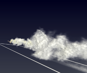
The instantaneous snapshots of the scalar field (figure 3) qualitatively show the effect of source elevation on the plume dispersion. The plume emitted by the ground-level source (e, f) does not meander significantly either vertically or horizontally and shows a larger instantaneous spread in the horizontal plane compared with the higher sources. The two elevated sources ( $z_s/\delta = 0.19$; figure 3(a,b), and $z_s/\delta = 0.5$; figure 3c,d) have similar visual characteristics, up to the downwind distance where the plume significantly impacts the ground, showing a narrow instantaneous plume with significant meandering motions. These visual differences among the sources are reflected in different statistics, as investigated below.
Instantaneous contour plot of scalar concentration  $\bar {c}^{*}$ from $6.25$ mm source in the ( $x,z$) plane (a,c,e) and ( $x,y$) plane (b,d, f) for (a,b) the elevated source at $z_s/\delta = 0.5$, (c,d) the elevated source at $z_s/\delta = 0.19$ and (e, f) the near-ground-level source.

4.1. Mean concentration field
The analysis of the mean concentration field is a prerequisite to appreciate, understand and discuss the spatial evolution of the higher statistical moments of the concentration fluctuations. Figure 4(a) shows the downwind variation of the centreline maximum of mean concentration for the investigated source sizes and elevations. Following Nironi et al. (Reference Nironi, Salizzoni, Marro, Mejean, Grosjean and Soulhac2015), the concentrations are normalised as  $\bar {c}^{*} = \bar {c} (u_s \delta ^2 / Q)$, where $Q$ indicates the source mass flow rate and $u_s$ the mean wind velocity at the source height $z_s$. Note that the concentration has here the dimension of mass per volume, as customary in atmospheric dispersion modelling (e.g. Panofsky & Dutton Reference Panofsky and Dutton1988; Arya Reference Arya1999). The first thing to be observed is that smaller source sizes imply initially higher concentrations, but this effect is short-lived as expected (e.g. Arya Reference Arya1999). The elevated sources, D6M and D12M, have indistinguishable centreline mean concentrations for $x / \delta \gtrapprox 0.5$, while the difference between D6 and D12 is negligible already at $x / \delta \approx 0.25$. This is due to the higher turbulence and lower mean wind speed at $z_s / \delta = 0.19$, compared with the core of the boundary layer. The situation is more complicated for the ground-level sources. Sources D6G-X and D12G become quite similar already at $x / \delta \approx 0.15$, while the mean concentrations for D6G and D12G intersect at $x / \delta \approx 0.3$, but the difference between the two persists at larger distances, with D6G having a slightly lower mean concentration.
(a) The along-wind variation of the maximum of the normalised mean concentration. (b) The along-wind variation of the crosswind centreline maximum of the normalised standard deviation of the concentration. The insets show the near-field region. Note that in this and the following figures the markers on the LES data are included to help the reader to distinguish more easily the different cases one from the other and do not correspond to sampling points.

The persistence of this gap can be explained by the differences in the source centreline heights. Although both sources are located close to the ground, D12G spans a larger vertical extension than D6G. This implies that the plume released from D12G is subject to a higher overall mean wind speed, which generates a slightly faster advection. This condition makes the advection of D12G similar to that of D6G-X (which has a slightly higher elevation; see table 1). Therefore, while differences in source size disappear quite quickly, even a small difference in the source elevations ( $\Delta z_s$) can result in persistent differences if $\Delta z_s$ is located in the high mean wind shear region, typical of a near-ground neutral boundary layer.
Note also that, at downwind distances  $x/\delta \gtrapprox 0.6$, the ground-level sources display higher values in the mean concentration compared with the elevated sources because of the zero-flux condition at the wall.
In the following, we also compare scalar concentration results of the LES and wind-tunnel experimental results, obtained in flows with different  $u_s$ and $u_{*}$. For the elevated sources, to avoid differences trivially arising due to varying advection times, we compare profiles taken at distances implying the same dimensionless advection time, $T^{*}=({x}/{u_s})({u_{*}}/{\delta })$, as suggested by e.g. Nironi et al. (Reference Nironi, Salizzoni, Marro, Mejean, Grosjean and Soulhac2015). Following the approach of Ardeshiri et al. (Reference Ardeshiri, Cassiani, Park, Stohl, Stebel, Pisso and Dinger2020) and looking for $T_{(exp)}^{*}=T_{(LES)}^{*}$ (where $exp$ stands here for experimental), we define therefore an equivalent along-wind distance as
 \begin{equation} x^* = \begin{cases} x & \text{(LES)}, \\ x\dfrac{u_{s(LES)}}{u_{s(exp)}} \dfrac{u_{*(exp)}}{u_{*(LES)}} & \text{(wind-tunnel experiments)}. \end{cases} \end{equation}
This approach is not used when considering plumes emitted by low-level sources, since it relies on the validity of Taylor's frozen turbulence hypothesis,  $(x = u_s t)$, which is questionable in regions of strong wind shear, where the along-wind turbulence standard deviation is not negligible compared with the mean wind. Therefore, for ground-level sources, it is simply $x^*=x$.
Figure 5 shows the crosswind (panels a–c) and vertical (panels d–f) profiles of the mean concentration  $\langle \bar {c} \rangle$ (including data by Nironi et al. (Reference Nironi, Salizzoni, Marro, Mejean, Grosjean and Soulhac2015) for $z_s = 0.19 \delta$), through the crosswind centreline for three different along-wind distances from the source. Figure 5(g,h) reports the normalised plume dispersion standard deviations in the crosswind $\sigma _y$ and vertical $\sigma _z$ directions (whose definition is given in Appendix B). As expected (e.g. Csanady Reference Csanady1973; Fackrell & Robins Reference Fackrell and Robins1982; Arya Reference Arya1999), the crosswind mean concentration profiles (figure 5a–c) are very well fitted by a Gaussian model (not shown here). The vertical profiles (figure 5d–f) are instead well modelled by a reflected Gaussian model, as evidenced by the Gaussian-D6G fit displayed in figure 5(d–f) for the near-ground source (see Appendix B for details about the reflected Gaussian formulation).
Profiles of the mean concentration in the (a–c) crosswind ( $z=z_s$) and (d–f) vertical direction at downwind distances (a,d) $x^*/\delta =0.36$, (b,e) $x^*/\delta =0.73$ and (c, f) $x^*/\delta =2.9$. The source size in Nironi et al. (Reference Nironi, Salizzoni, Marro, Mejean, Grosjean and Soulhac2015) data is $d_s=6\ {\rm mm}=0.0075\delta$ and the source elevation is $z_s/\delta = 0.19$. Panels (g,h) report the LES plume spatial standard deviation in crosswind $\sigma _y$ and vertical $\sigma _z$ directions as a function of downwind distance for both the 6.25 mm and 12.5 mm sources together with Nironi et al. (Reference Nironi, Salizzoni, Marro, Mejean, Grosjean and Soulhac2015) data for the 6 mm source. For ground-level sources in the vertical direction, the definition of $\sigma _z$ is explained in Appendix B, together with the definition of the Gaussian approximation for D6G.

For the downwind distances displayed in figure 5, and in agreement with what was discussed above for figure 4, the mean concentration profile is very weakly affected by a varying source size, whose influence can be detected only very close to the emission (e.g. D6M and D12M at  $x^*/ \delta = 0.36$; figure 5a,d). In contrast, the source elevation significantly alters the mean concentration. Plumes emitted by sources at mid-height have a higher maximum mean concentration than those at $z_s/\delta =0.19$, at all downwind distances (figures 4a and 5a–f). This can be readily explained through a plume Gaussian model ((B3) in Appendix B): increasing $z_s$, the mean wind speed increases and, therefore, the plume travel time shortens. In this case $u_s = 4.4\ {\rm m}\ {\rm s}^{-1}$ in the middle of the boundary layer (D6M and D12M), whereas $u_s = 3.8 \ {\rm m}\ {\rm s}^{-1}$ at $z_s/ \delta = 0.19$. Furthermore, the turbulent fluctuations decrease with height (see figure 1e, f). These two aspects have a considerable impact on the plume spreads $\sigma _y$ and $\sigma _z$ (figure 5g,h) and, therefore, on $\langle c^*\rangle$. The ground-level sources present a more complex behaviour. At $x^*/\delta = 0.36$, the ground-level sources show a higher mean concentration than those of the sources at $z_s/ \delta =0.19$ but lower than the mean concentration of the sources at $z_s/ \delta =0.5$, as shown in figure 5(a,d). For downwind distances $x^*/\delta \gtrapprox 0.6$, the mean concentration of the ground-level sources are always the highest among the simulated configurations (figure 4a and 5b,c,e, f). In these cases, although the plume travel times are longer compared with the elevated sources, the ground effect has a prevalent role and produces a lower plume dispersion. The difference between the mean concentration of D6G and D12G arises, as discussed above in relation to figure 4, from the different top vertical extension of the two sources. As in previous studies (Fackrell & Robins Reference Fackrell and Robins1982; Crimaldi & Koseff Reference Crimaldi and Koseff2006), power laws are fitted to the plume standard deviations (figure 5g,h). For the source at $z_s/\delta = 0.5$, $\sigma _y \propto x^{0.86}$ and $\sigma _z \propto x^{0.85}$. For $z_s/\delta = 0.19$, $\sigma _z \propto x^{0.74}$ and $\sigma _y \propto x^{0.8}$. For near-ground sources $\sigma _z \propto x^{0.77}$, a value similar to that obtained by F&R and Crimaldi & Koseff (Reference Crimaldi and Koseff2006) and $\sigma _y \propto x^{0.67}$. This latter is due to the longer advection time and to the smaller size of near-ground turbulent structures, resulting in a more diffusive regime. The value of the exponent of the power law does not exhibit significant dependencies on the source size.
Overall, the good quantitative match with the measurements of Nironi et al. (Reference Nironi, Salizzoni, Marro, Mejean, Grosjean and Soulhac2015) and the general consistency with the data reported in Talluru et al. (Reference Talluru, Philip and Chauhan2018) for sources in the same range of elevations, show the reliability of the LES.
Finally note that, in the case of a large Schmidt number ( $Sc=\nu /D)$, ground-level source releases in smooth walls get trapped in the viscous layer (Crimaldi, Wiley & Koseff Reference Crimaldi, Wiley and Koseff2002; Lim & Vanderwel Reference Lim and Vanderwel2023). This phenomenon fades out both for lower values of $Sc$ (e.g. Talluru et al. Reference Talluru, Philip and Chauhan2018) and for rough walls, and cannot therefore be simulated in our LES.
4.2. Concentration fluctuations standard deviation
Differently from the mean, the standard deviation of the concentration fluctuations ( $\sigma _c^{*}$) is strongly affected by the source size for the elevated sources, whereas the effects on the ground-level sources are less evident (e.g. Fackrell & Robins Reference Fackrell and Robins1982; Thomson Reference Thomson1990; Cassiani et al. Reference Cassiani, Franzese and Giostra2005). As extensively discussed in Ardeshiri et al. (Reference Ardeshiri, Cassiani, Park, Stohl, Stebel, Pisso and Dinger2020), the generation of the fluctuations for a plume emitted by an elevated source is dominated by the early phases of plume dispersion that are characterised by the meandering motion (Gifford Reference Gifford1959) of the almost unmixed plume. We briefly recall here that the concentration fluctuations are driven by two phenomena: the meandering movement of the instantaneous plume (Gifford Reference Gifford1959; Csanady Reference Csanady1973; Cassiani & Giostra Reference Cassiani and Giostra2002; Cassiani et al. Reference Cassiani, Bertagni, Marro and Salizzoni2020) displacing the plume's centre of mass, and the dispersion (expansion) of the plume relative to the centre of mass (Sawford Reference Sawford2001; Dosio & de Arellano Reference Dosio and de Arellano2006; Franzese & Cassiani Reference Franzese and Cassiani2007; Cassiani et al. Reference Cassiani, Bertagni, Marro and Salizzoni2020).
Since turbulence is characterised by eddies with a wide range of temporal and spatial scales, if the source is small, a larger range of scales can contribute to the meandering motion of the plume compared with its relative dispersion. This implies that the concentration fluctuations increase with decreasing source size.
Moving downwind from the source, the initial difference in the (crosswind and vertical) dimension of the plumes relative to their centre of mass (i.e. the relative dispersion) becomes progressively negligible compared with the growing plume cross-section, and the source-size effect is progressively lost.
This behaviour is well confirmed for the elevated sources by figures 4(b) and 6, which show that, close to the emission point, D6 (or D6M) presents higher values of  $\sigma _c^*$ compared with D12 (or D12M). These differences disappear, respectively, at $x/ \delta \approx 1.8$ for the sources at $z_s = 0.19 \delta$ and at $x/ \delta \approx 3.4$ for the sources in the middle of the boundary layer. The ground-level sources exhibit some noticeable differences in the concentration variance only in the very near-source region, and these differences rapidly vanish at $x/\delta \approx 0.4$ (see figure 4b).
(a–c) Transversal and (d–f) vertical profiles of concentration fluctuations standard deviation at various downwind distances: (a,d)  $x^*/\delta =0.36$ (b,e) $x^*/\delta =0.73$ and (c, f) $x^*/\delta =2.9$.

The greater persistence of the differences in  $\sigma _c^*$ with the increase of the source elevation is due to several reasons: (i) the higher mean wind speed, meaning that the plume has a shorter travel time to evolve, (ii) the higher initial production of fluctuations due to meandering, and (iii) the less intense dissipation rate of the scalar variance.
The reader should note in figures 4(b) and 6 that the slight difference in elevation between D6G and D6G-X has a small influence on the value of the concentration standard deviation.
Regarding the direct quantitative comparison with the wind-tunnel experiments, similarly to what was done for the mean concentration, we limit it to the measurements for the  $6\ {\rm mm}$ source at $z_s / \delta = 0.19$ in Nironi et al. (Reference Nironi, Salizzoni, Marro, Mejean, Grosjean and Soulhac2015). Compared with the wind-tunnel data, the simulations display a slightly higher concentration standard deviation. We believe that this is due to a combination of factors. The effective source diameter in Nironi et al. (Reference Nironi, Salizzoni, Marro, Mejean, Grosjean and Soulhac2015) should be considered equal to the external diameter of the pipe emitting the scalar ( $8\ {\rm mm}$), rather than its internal diameter, i.e. $6\ {\rm mm}$. Furthermore, even though the gas is emitted isokinetically, the physical presence of the source in the experiments induces a wake perturbing the flow locally, an effect that is not reproduced in the LES, where the source is just a marker. Finally, the differences in the turbulent flow between Nironi et al. (Reference Nironi, Salizzoni, Marro, Mejean, Grosjean and Soulhac2015) and our simulations (see figures 1 and 2) are likely to contribute to the discrepancies observed in the concentration fields.
A general, although more qualitative, comparison of our results in figure 6 is possible with the measurements of Talluru et al. (Reference Talluru, Philip and Chauhan2018), showing substantial consistency in the spatial profiles of  $\sigma _c^*$ for the elevated sources. For the ground-level source, the observations of Talluru et al. (Reference Talluru, Philip and Chauhan2018) at $x/\delta = 1$ showed a vertical profile similar to those observed in our simulations in figure 6, with minimal difference between the peak value and the ground value. Overall, the comparison with the wind-tunnel experiments confirms confidence in the current simulations.
In the downwind range of our simulations, the horizontal crosswind profiles of concentration fluctuations for the ground-level sources show a persistent double-peak behaviour regardless of the distance from the source location. In contrast, for the elevated sources, this behaviour is observed only in the vicinity of the source and is not visible in the range of downwind distances reported in figure 6. This feature will be further investigated in the following section.
4.2.1. Double-peak behaviour in the very near-source region
The horizontal crosswind profile of the concentration standard deviation generated by a plume shows a double-peak behaviour very close to the source ( $x/\delta < 0.05$), irrespective of the source size and elevation, as illustrated in figure 7. The appropriate grid resolution of the simulations allows us to immediately capture the off-centre variance peaks very near the source location. Note that this was not possible in the previous study of Xie et al. (Reference Xie, Hayden, Voke and Robins2004b) due to the too coarse spatial discretisation. The bimodal shape of the variance profiles has seldom been observed in previous experimental studies of point sources, as operational conditions, such as the presence of the stack, could influence the very near scalar field. For elevated sources, this behaviour disappears particularly rapidly for smaller sources and is not visible already at $x / \delta = 0.15$ for both D6M and D6. For D12, the double peak disappears between $x/ \delta = 0.1$ and $x/ \delta = 0.15$ while, for D12M, it is still weakly visible at $x/ \delta = 0.2$ due to the faster advection and shorter plume travel time. For ground-level sources, the double peak appears to be persistent in the downwind range of our simulations, although initially, it is less pronounced than for the elevated sources. Figure 7 also confirms that initially the standard deviation of D6G is significantly larger than that of D12G, but this difference decreases very rapidly. For the elevated sources, the double peak is also present in the vertical direction (not shown here) and is similar to the crosswind profile since the plume development initially has an almost radial symmetry due to the similar statistics of the $v$ and $w$ velocity components. Conversely, for the ground-level sources, the double peak is not observable in the vertical section.
Transversal profiles of concentration fluctuations standard deviation in the vicinity of the source: (a)  $x/\delta =0.05$ (b) $x/\delta =0.10$ (c) $x/\delta =0.15$ and (d) $x/\delta =0.20$.

The generation and time evolution of the double peak in  $\sigma _c$ have been studied using stochastic models and theoretically by Thomson (Reference Thomson1990, Reference Thomson1996) for instantaneous scalar releases (line source) in homogeneous turbulence with no mean advection. This case can be interpreted as a continuous plume in an approximately homogeneous turbulent flow (i.e. similar to our elevated plume dispersion cases) in the presence of mean advection by adopting Taylor's approximation to transform between plume evolution in a downwind position and time. Thomson (Reference Thomson1996) argued that the off-centre variance peaks disappear when the absolute dispersion scale becomes of the order of the source size, i.e. when the total average plume size, including the source, doubles, $\sigma _y/\sigma _s \approx 2$ in the present context, where $\sigma _s$ is the LES source size calculated as the actual plume standard deviation at the source location. Following the concentration fluctuation profiles in the along-wind direction, the approximate distances where the double-peak behaviour vanishes in the LES are reported in table 2, showing that the findings of Thomson (Reference Thomson1996) are satisfied with good approximation. Furthermore, Thomson (Reference Thomson1996) argued that the overall peak in $\sigma _c$ occurs for $\sigma _y/\sigma _s \approx 2$. Looking at figure 7, particularly for D12M, which evolves slower and is therefore better resolved at the considered time intervals, the overall peak in $\sigma _c$ slightly increases in $x/\delta = 0.05-0.1$, it remains approximately constant in the interval $x/\delta = 0.1-0.15$, and it slightly decreases for $x/\delta = 0.15-0.2$. This reasonably agrees with Thomson (Reference Thomson1996).
Distance  $x/\delta |_{LES}$ of the disappearance of the double peak in $\sigma _c^*$ for the elevated plumes and the corresponding plume size expressed as $\sigma _y/ \sigma _s$.

For the ground-level source, the off-centre double peaks appear to be persistent in the downwind range of the simulations. In order to better understand the differences between the generation of concentration fluctuations for ground-level and elevated sources, the budget equation for the resolved scale mean scalar variance is considered:
 \begin{equation} 0 = \underbrace{-\langle\bar{u}_i \rangle \frac{\partial \langle \bar{c}''^2\rangle}{\partial x_i}}_\text{Adv.} \underbrace{- 2\langle \bar{u}_i''\bar{c}''\rangle \frac{\partial \langle \bar{c}\rangle}{\partial x_i}}_\text{Prod.} \underbrace{-\frac{\partial \langle \bar{u}_i''\bar{c}''^2 \rangle}{\partial x_i}}_\text{T.T.} - 2 \xi_{res}. \end{equation}
 Here the first term on the right-hand side corresponds to the advection (Adv.), the second and third terms correspond to the production (Prod.) and turbulent transport (T.T.), respectively, and  $\xi _{res}$ is the mean scalar dissipation rate computed as the residual. The factor $2$ is left explicit in analogy with what appears in the definition of the actual physical dissipation, i.e. $2 \nu _c \langle {({\partial {c''}}/{\partial x_i})({\partial {c''}}/{\partial x_i})} \rangle$, where $\nu _c$ here is the molecular diffusivity. Heinze, Mironov & Raasch (Reference Heinze, Mironov and Raasch2015) and Ardeshiri et al. (Reference Ardeshiri, Cassiani, Park, Stohl, Stebel, Pisso and Dinger2020) discussed in detail that for the numerical methods used in the PALM code, due to the numerical dissipation, other estimates of the mean scalar dissipation rate, like the equilibrium approximation for the SGS (see e.g. Sykes & Henn Reference Sykes and Henn1992; Kaul et al. Reference Kaul, Raman, Balarac and Pitsch2009) and the transfer of resolved scale scalar variance to the SGS (see e.g. Heinze et al. Reference Heinze, Mironov and Raasch2015), do not correctly represent the actual dissipation rate.Kewley (Reference Kewley1978) showed that an approximate solution of the concentration variance transport equation is possible based on a balance between the production and dissipation rates. This approximation produces a double-peak profile (see also Netterville Reference Netterville1979) with a concentration variance value of zero at the plume centreline. The turbulent transport acts to smooth this double peak towards a Gaussian-like behaviour and produces non-zero concentration variance along the plume centreline. Figure 8 shows the budget (for the 12.5 mm sources) at the elevation of maximum mean concentration in the crosswind direction. The budget terms are generically indicated as $\phi$ and reported normalised as $\phi ^{*} = \phi (\delta / u_{*}) (u_s \delta ^2 / Q)^2$. Figure 8 reveals that the production terms for both ground-level and elevated sources exhibit a clear persistent double peak. Initially, the double peak is more pronounced for the elevated sources (see figure 7 at $x/\delta$ =0.1 and 0.15) and this is in agreement with the more pronounced double-peak behaviour in the production term for the elevated sources. However, for the ground-level sources, this term remains relevant with increasing downwind distance from the source, while for the elevated sources, it becomes negligible at $x/\delta = 0.625$. The more persistent relevance for the ground-level sources is mainly due to a stronger decay of the advection term, which becomes the dominant term for the higher elevations. This behaviour is consistent with the experimental observations of F&R.
Variance budget analysis of scalar concentration. Here  $\phi ^{*}$ represents a generic normalised quantity in (4.2) as a function of crosswind direction ( $y / \delta$) and for the $12.5$ mm source at (a) $z_s/\delta =0.003$ (D12G) (b) $z_s/\delta =0.19$ (D12) and (c) $z_s/\delta =0.5$ (D12M) and at a downwind distance of $x/\delta =0.13$. Panels (d–f) report the same quantities as (a–c) but at $x/\delta =0.625$.

4.3. Characteristics of the most energetic scales in the concentration variance power spectrum
To gain further insights into the mechanics of the scalar dispersion process, we investigate the variance-containing range of the concentration power spectrum,  $\varPhi _{cc}$ (see Appendix A). First, the LES results for the elevated sources will be discussed and afterwards theoretical arguments based on a stochastic approach will be used to show the connection between the peak in the variance-containing range of $\varPhi _{cc}$ and the peak in the energy-containing range of $\varPhi _{vv}$ and $\varPhi _{ww}$ in relation to the meandering motion of the plume. The section concludes with a qualitative analysis of the shape of the variance-containing range for the ground-level sources.
The spectra are normalised by the concentration variance and smoothed using a Gaussian filter, as they would otherwise be affected by noise hindering the clear detection of the shape. We observe that, for constant downwind distances and a given source elevation, the pre-multiplied normalised spectra ( $f\varPhi _{cc}/\sigma _c^2$) tend to exhibit a common shape, independent of the sampling position in the $(y,z)$ plane (figure 9). We remind the reader that the frequency of the peak in the pre-multiplied spectrum is directly related to the integral scale (see Appendix A).
Pre-multiplied normalised energy spectrum of the concentration fluctuations as a function of normalised frequency for three downwind distances and two source elevations. Results are shown for (a,b,c,g,h,i)  $z_s = 0.5 \delta$ and (d,e, f,j,k,l) $z_s = 0.19 \delta$. Spectra sampled at several vertical positions for $y=y_s$ (a–f) and spectra sampled at several crosswind lateral positions for $z=z_s$ (g–l).

Note that all the reported sampling points, for a given downwind distance  $x$, are characterised by a mean concentration $\langle c^* \rangle (y=y_s,z) > {\langle c^* \rangle }_ {max} / 50$ or $\langle c^* \rangle (y,z=z_s) > {\langle c^* \rangle }_ {max} / 50$, which identifies a distance of approximately two standard deviations, on the axis, from the local mean plume centreline. At a greater distance from the plume centreline, the sampled time series are too short (given the high level of fluctuations) to obtain reliable spectra.
The common shape of the most energetic part of the pre-multiplied normalised concentration fluctuation spectra was originally noted in Talluru et al. (Reference Talluru, Philip and Chauhan2019).
The results in panel ( f) ( $z_s/\delta = 0.19$) at $y=y_s$, $z / \delta = 0.024$, $x/\delta =2.51$ show that the spectra do not follow the common curve at this low elevation, as the plume has a large vertical extension (see e.g. figure 5g,h) and the time series is sampled close to the ground, where the turbulence characteristics are significantly different from those in the source region, as reported in figure 1. This anticipates that the spectra computed for the ground-level sources cannot be invariant.
The common shape of the normalised pre-multiplied concentration variance spectra for elevated sources was motivated by Talluru et al. (Reference Talluru, Philip and Chauhan2019), arguing that it is controlled by large-scale flow properties driving the plume meandering. Our data in figure 9 show that the shape of the pre-multiplied normalised spectra changes with the downwind distance, including a shift of the spectral peak towards lower frequencies and, consequently, a change in the integral time scales. This behaviour is consistent with the literature on plume dispersion, which relates concentration fluctuations to the meandering of the plume, as it also expands through a relative dispersion process with increasing downwind distance (e.g. Hanna Reference Hanna1986; Hanna & Insley Reference Hanna and Insley1989; Sawford Reference Sawford2001; Ardeshiri et al. Reference Ardeshiri, Cassiani, Park, Stohl, Stebel, Pisso and Dinger2020; Cassiani et al. Reference Cassiani, Bertagni, Marro and Salizzoni2020) and will be investigated in the next section.
4.3.1. Analysis of the spectra using velocity conditioned stochastic time series for elevated sources
Following the evidence of our LES data and the customary interpretation of concentration fluctuations by meandering and relative dispersion, we provide here a quantitative explanation of the relation between the velocity and concentration time scales. We remind the reader that the spectral peak is directly related to the time scale (e.g. Kaimal & Finnigan Reference Kaimal and Finnigan1994), as explained in Appendix A.
Our analysis is based on the ideas of Cassiani et al. (Reference Cassiani, Franzese and Albertson2009) that the concentration fluctuations time series at a fixed point in space, and therefore its spectrum, are characterised by two time scales, one related to the meandering of the expanding plume, which can be directly connected to the time scales of crosswind and vertical velocities through a conditional average meandering model, and the other to the scalar dissipation rate. For a slender plume, and using Taylor's hypothesis, the mean concentration field from an elevated source is well described by a Gaussian model ((B3) in Appendix B) when neglecting any ground effect. A good approximation for the elevated source plume is also the assumption of homogeneous anisotropic turbulence, with the turbulence statistics sampled at the source location. This assumption allows us to describe the standard deviations of the plume spread in the vertical and crosswind directions according to Taylor (Reference Taylor1922) theory:
 \begin{equation} \left. \begin{gathered} \sigma_{y}^2 = \sigma_s^2 + \sigma_v^2 T_{Lv}^2 \left[2\frac{t}{T_{Lv}} - 2\left(1-\exp\left(-\frac{t}{T_{Lv}}\right) \right) \right],\\ \sigma_{z}^2 = \sigma_s^2 + \sigma_w^2 T_{Lw}^2 \left[2\frac{t}{T_{Lw}} - 2\left(1-\exp\left(-\frac{t}{T_{Lw}}\right) \right) \right], \end{gathered} \right\} \end{equation}
where  $\sigma _s$ is the source size, and $T_{Lv}$ and $T_{Lw}$ are here the crosswind and vertical Lagrangian integral time scales, respectively (e.g. Arya Reference Arya1999). For elevated sources, these equations can be fit to the LES plume dispersion variances (e.g. Ardeshiri et al. Reference Ardeshiri, Cassiani, Park, Stohl, Stebel, Pisso and Dinger2020).
Therefore, we use here the semi-analytical approach originally proposed in Sawford (Reference Sawford2004) and Cassiani et al. (Reference Cassiani, Franzese and Albertson2009) to analyse dispersion from a line source in grid turbulence but extending it here to a point source with two-dimensional dispersion. Following Cassiani et al. (Reference Cassiani, Franzese and Albertson2009) a stochastic model for the concentration time series incorporating meandering can be defined as
 $$\begin{gather} {\rm d}v ={-} \frac{v}{T_{v}} \,{\rm d}t + \left(\frac{2 \sigma_v^2}{T_{v}} \right)^{1/2} \,{\rm d}W_v, \end{gather}$$
 $$\begin{gather}{\rm d}w ={-} \frac{w}{T_{w}} \,{\rm d}t + \left(\frac{2 \sigma_w^2}{T_{w}} \right)^{1/2} \,{\rm d}W_w, \end{gather}$$
 $$\begin{gather}{\rm d}c ={-} \frac{c-\left\langle c\mid v,w \right\rangle}{T_s}\,{\rm d}t + g(c,T_s^{{-}1},\left\langle\left\langle c\mid v,w \right\rangle \mid c \right\rangle, f_c) \,{\rm d}W_c, \end{gather}$$
where  $\textrm {d}W_{v}$, $\textrm {d}W_w$ and $\textrm {d}W_c$ are independent Wiener process (see e.g. Pope Reference Pope2000). The use of a simple Langevin model for the velocity components allows for an unambiguous relationship between the spectral peaks and the time scales $T_{v}$ and $T_{w}$. These time scales are selected here from the spectral peak frequency at the plume source elevation, as identified in figure 2(h,i), using the relation $fm_{i} = 1/(2 {\rm \pi}T_{i})$ (e.g. Kaimal & Finnigan Reference Kaimal and Finnigan1994, see also Appendix A). Equation (4.4c) is the most general formulation of the concentration time series evolution proposed in Cassiani et al. (Reference Cassiani, Franzese and Albertson2009), but here we significantly simplify this model by neglecting the stochastic diffusion term (function $g$ above) because it is not necessary for our analysis. The diffusion term allows the correct fluctuations of concentration far downwind from the source where the plume meandering is negligible (Cassiani et al. Reference Cassiani, Franzese and Albertson2009), while it is unimportant close to the source where the meandering dominates. The interested reader may find the explicit formulation of the diffusion term in Cassiani et al. (Reference Cassiani, Franzese and Albertson2009). Nonetheless, it is instrumental for the present analysis to underline that the explicit form contains only one time scale $T_s$, the same time scale contained in the drift (relaxation) term in (4.4c). In the drift term, the instantaneous concentration relaxes towards $\langle c\mid v,w \rangle$, which is the local mean concentration conditioned over the crosswind and vertical velocity components. At short travel time from the source location, $T_s \rightarrow 0$ (Cassiani et al. Reference Cassiani, Franzese and Albertson2009) and the instantaneous concentration in (4.4c) can be significantly simplified as
 \begin{equation} c= \left\langle c\mid v,w \right\rangle. \end{equation}
Sawford (Reference Sawford2004) demonstrated that this definition of the instantaneous concentration corresponds to the concentration generated by a meandering plume model where the relative dispersion ( $\sigma _r$) is modelled as $\sigma _{ry}^2 = \sigma _s^2 + \sigma _y^2(1-\rho _{vy}^2)$ for the crosswind direction, and $\sigma _{rz}^2 = \sigma _s^2 + \sigma _z^2(1-\rho _{wz}^2)$ for the vertical direction. The terms $\rho _{vy}$ and $\rho _{wz}$ represent the correlation between the velocity and the displacement $\Delta$ of a marked fluid particle passing through the source (Sawford Reference Sawford2004) and are defined as
 \begin{equation} \left. \begin{gathered} \rho_{vy} = \frac{\left\langle v \Delta y \right\rangle}{ \sigma_v \sigma_y}=\frac{1}{ 2 \sigma_v \sigma_y}\frac{{\rm d}\sigma_y^2}{ {\rm d}t},\\ \rho_{wz} = \frac{\left\langle w \Delta z \right\rangle}{ \sigma_w \sigma_z}=\frac{1}{ 2 \sigma_w \sigma_z}\frac{{\rm d} \sigma_z^2}{ {\rm d}t}. \end{gathered} \right\} \end{equation}
The analytical formulation of the conditional mean concentration can be obtained as (Sawford Reference Sawford2004)
 \begin{align}
\left\langle c(y,z,t) \mid v,w \right\rangle &= \frac{Q}{u_s
2{\rm \pi} ((\sigma_s^2 + \sigma_y^2 (1-\rho_{vy}^2))^{(1/2)} )
((\sigma_s^2 + \sigma_z^2 (1-\rho_{wz}^2))^{(1/2)} )}\nonumber\\
&\quad \times\exp\left(-\frac{(y-\rho_{vy} v \sigma_y / \sigma_v )^2}{2
(\sigma_s^2 + \sigma_y^2 (1-\rho_{vy}^2)) } \right)
\exp\left(-\frac{(z-\rho_{wz} w \sigma_z / \sigma_w )^2}{2
(\sigma_s^2 + \sigma_z^2 (1-\rho_{wz}^2)) } \right).
\end{align}
\begin{align}
\left\langle c(y,z,t) \mid v,w \right\rangle &= \frac{Q}{u_s
2{\rm \pi} ((\sigma_s^2 + \sigma_y^2 (1-\rho_{vy}^2))^{(1/2)} )
((\sigma_s^2 + \sigma_z^2 (1-\rho_{wz}^2))^{(1/2)} )}\nonumber\\
&\quad \times\exp\left(-\frac{(y-\rho_{vy} v \sigma_y / \sigma_v )^2}{2
(\sigma_s^2 + \sigma_y^2 (1-\rho_{vy}^2)) } \right)
\exp\left(-\frac{(z-\rho_{wz} w \sigma_z / \sigma_w )^2}{2
(\sigma_s^2 + \sigma_z^2 (1-\rho_{wz}^2)) } \right).
\end{align} The stochastic model defined by (4.4a,b), (4.5), (4.7) and (4.6) was applied using the LES flow data sampled at the source elevation,  $z_s / \delta = 0.5$, namely the velocity statistics and the time scales obtained from the spectral peaks, $fm$, as shown in figure 2(h,i): $T_w=1/(2{\rm \pi} fm_w)=0.14\delta /u_{\infty }$, $T_v=1/(2 {\rm \pi}fm_v)=0.17\delta /u_{\infty }$. The resulting spectra are plotted in figure 10 for the elevated source plume, $z_s = 0.5 \delta$, for which the hypotheses underlying this stochastic model are better respected. The $v$,
$v$,  $w$ and $c$ spectra at the downwind distance $x = 0.16 \delta$ are reported for different vertical and lateral positions, respectively, in panels (a,b). We are aware that the overall shape of the LES spectrum cannot be perfectly reproduced by a simple diffusive model, but the peaks in the velocity component spectra correspond, by construction, exactly to those extracted from figure 2(h,i) at the source elevation.
Pre-multiplied and normalised energy spectrum of velocity components and concentration obtained with the stochastic model for the source located at  $z_s=0.5\delta$. (a,b) Vertical and lateral variations of the spectrum at $x = 0.16 \delta$. (c) Vertical variation of the spectrum at $x = 2.51 \delta$. The different dashed lines correspond to different positions for the concentration time series stochastic model with respect to the plume centre. Panels (d–f) report the corresponding LES spectra for reader convenience.

Figure 10 shows a significant shift towards higher frequencies in the concentration spectra compared with the velocity components  $(u,w)$ in the stochastic theoretical model. This modelled behaviour is consistent with that observed in the LES data, i.e. comparing figure 2(h,i) (at the source plume elevation) with figure 9(a,g). The LES scalar spectra are also reported in figure 10(d–f) to facilitate comparison with the stochastic model. The results from the stochastic model show a very weak dependence of the spectra on the position in the crosswind plane, i.e. they do not show a complete overlap (irrespective of the sampling position in the crosswind plane) of the concentration spectra close to the source location ( $x = 0.16 \delta$). We note that at this location the meandering dominates the fluctuations and the conditional mean is a very good approximation of the instantaneous scalar field, allowing the conditional mean model to capture about $90\,\%$ of the actual concentration variance. A very weak dependence on the position in the crosswind plane cannot be ruled out also in the LES data in figure 10(d,e).
At larger distances from the release point, the conditional mean model for the meandering process becomes less precise. Furthermore, the fraction of actual variance that can be explained by the meandering of the plume decreases, while the concentration fluctuations generated by the entrainment process due to relative dispersion become more significant. Nonetheless, it is instructive to examine what happens to the spectra of fluctuations generated by the meandering process as the plume increases its relative dispersion. For this reason, the stochastic model was applied at the distance  $x = 2.51 \delta$, although the model is able to explain only a small fraction of the actual concentration variance at this location. We observe that the concentration spectral peak shifts to $1 < f \delta /u_{\infty } < 2$ (figure 10c), which is consistent with the LES data reported in figure 9(c) and in figure 10( f). However, the spectra generated by the LES display a better collapse onto a unique curve, while the stochastic model based on the conditional mean approximation shows a small but clear shift of the spectra depending on the vertical sampling position. We can argue that the fluctuations due to relative dispersion, which are not accounted for by the meandering model, enhance the similarity in the concentration spectra since they are associated with a unique time scale (Cassiani et al. Reference Cassiani, Franzese and Albertson2009), $T_s$ in (4.4). The scalar time $T_s$ becomes increasingly relevant as one moves downwind from the source. However, the exact value of $T_s$ is not known a priori and requires a model itself. Cassiani et al. (Reference Cassiani, Franzese and Albertson2009) considered $T_s \propto T_m \propto T_{\phi } = \sigma _c^2 / \xi$, where $T_m$ is the Lagrangian mixing time scale usually considered proportional to the scalar dissipation rate time scale $T_{\phi }$ ( $\xi$ is the scalar dissipation rate defined here as the residual in (4.2) for the special case of the LES simulation) as extensively reviewed in e.g. Cassiani et al. (Reference Cassiani, Bertagni, Marro and Salizzoni2020). Therefore, to further investigate the level of similarity in the spectrum, we calculated the scalar dissipation rate time scale $T_{\phi }$ from the LES data, under the assumption that $T_s$ and $T_{\phi }$ are proportional. Figure 11 shows $T_\phi$ as a function of both crosswind and vertical positions for the plume released at $z_s = 0.5\delta$ at varying distances from the source locations. The dissipation rate time scale is approximately independent of the $y$ and $z$ coordinates (for a fixed value of $x/\delta$) and increases with the downwind distance as expected. The time scale $T_s$ should exhibit the same behaviour, assuming that it is proportional to $T_{\phi }$, as hypothesised in Cassiani et al. (Reference Cassiani, Franzese and Albertson2009).
Dissipation time scale  $T_\phi$ scaled by $\delta / u_{\infty }$ for the source at $z_s = 0.5 \delta$. (a) Variation along the vertical direction for four downwind distances. Panel (b) is the same as (a) but for the crosswind direction. Lateral and vertical coordinates are normalised for the plume standard deviations.

Summarising, for a given position, the concentration time series are influenced by the conditional mean  $\langle c\mid v,w \rangle$, which generates a spectral peak (and corresponding time scale) that depends weakly on the sampling point for a fixed downwind distance, and on the time scale $T_s$ that seems to be constant in the $(y,z)$ plane. As the plume travel time increases, both time scales grow and the concentration progressively switches from a direct dependence on the conditional mean to a dependence mediated by the time scale $T_s$, which enhances the similarity of the spectrum.
This discussion supports the evidence that the spectral peak in the concentration spectrum (and the related time scales) must necessarily shift towards lower frequencies as the downwind distance increases, being, however, independent (or weakly dependent) of the sampling position in the  $(y,z)$ plane (for a fixed travel time). Moreover, such a shift is directly linked to the relative dispersion process and, therefore, to the actual (instantaneous) plume size.
There are some aspects that deserve further discussion. At first glance, one might be tempted to relate the dissipation time scale  $T_\phi$ directly to $T_s$ or even to the spectral peak observed in the LES by a relation of the form $fm_{\alpha } \cong 1/(2 {\rm \pi}T_{\alpha })$. However, $T_s$ and the spectral peaks in figure 10 are related to Eulerian time series in the presence of a mean wind field, while $T_\phi$ is a physical time scale similar to the turbulent flow time scale $E/\epsilon$, where $E= 1/2 (\sigma _u^2(z) + \sigma _v^2(z) + \sigma _w^2(z))$ is the turbulent kinetic energy and $\epsilon$ is its dissipation rate (e.g. Pope Reference Pope2000). These physical time scales are unrelated to the mean advecting wind and are indeed more similar to Lagrangian integral scales. In the presence of a mean wind field, the relation between the Eulerian and the Lagrangian time scales ( $T_E$ and $T_L$) involves the turbulence intensity, $E^{1/2}/\langle u \rangle$, with $T_E \propto T_L E^{1/2} /\langle u \rangle$ (e.g. Arya Reference Arya1999; Cassiani et al. Reference Cassiani, Franzese and Albertson2009). For a neutral boundary layer, the turbulence intensity at the considered source and plume elevation is ${\ll }1$, and we may expect that the time scale corresponding to the concentration time series is much shorter compared with that of the dissipation process, i.e. $T_s \ll T_{\phi }$. The aforementioned scalar time scales are generally assumed to exhibit a very weak dependence on the Schmidt number (Fox Reference Fox2003), which is usually neglected in scalar dispersion models (see Cassiani et al. Reference Cassiani, Bertagni, Marro and Salizzoni2020).
4.3.2. LES spectra of concentration fluctuations for ground-level sources
The concentration spectra of a ground-level source (figure 12) present a strong dependence on the vertical position. Their shape changes significantly with elevation, and the spectral peak of  $\varPhi _{cc}$ shifts from low to high frequency. This reflects the high vertical inhomogeneity. In figure 12 the vertical lines bound the location of the spectral peak of $f\varPhi _{uu}$ for $z/\delta > 0.011 \delta$ above the sharp transition at $z/\delta \approx 0.01$, which moves the peak from the high frequencies to the low frequencies (see also figure 2g,d).
Pre-multiplied normalised energy spectrum of the concentration fluctuations as a function of normalised frequency for the ground-level source D6G at three downwind distances. Spectra sampled at several vertical positions for  $y=y_s$. The vertical blue lines bound the location of the spectral peak of $f\varPhi _{uu}$ for $z/\delta \gtrapprox 0.011$.

We observe that the frequency location of the peak at low vertical positions (figure 12) is in a very similar location when compared with the peak in the spectrum of the along-wind velocity fluctuations  $\varPhi _{uu}$ for $z/\delta > 0.01$ (figure 2g). Moving vertically towards the plume edges the spectral peak location in $\varPhi _{cc}$ shifts to the high frequencies that are similar to what was previously investigated for the elevated sources. This feature is related to the meandering motions and is linked to the spectra of the $v$ and $w$ velocity components, as discussed above in § 4.3.1.
This peak transition from low to high frequencies occurs at higher vertical positions as the distance from the source location increases. Such behaviour suggests that this shift is not related to the flow properties but to the plume dispersion and its vertical size. As a first approximation, we estimate the transition at  $z\approx 2 \sigma _z$ from the ground.
We speculate that away from the ground, where the entrainment process creates plume filaments, the fluctuations are dominated by meandering motions in the directions orthogonal to the mean wind flow ( $(y,z)$ plane). On the contrary this process is negligible for the plume main body (defined here as $z \lessapprox 2 \sigma _z$) from the ground and the fluctuations are instead generated by the actions of the along-wind turbulence, and therefore, the peak is at a lower frequency.
4.4. Higher-order central moments and scalar p.d.f.
Analysis of the high-order statistics focuses on the skewness and kurtosis of the concentration. Furthermore, we also report the spatial evolution of the fluctuation intensity  $i_c=\sigma _c / \langle c \rangle$, since it is generally a key parameter for modelling the scalar p.d.f. (e.g. Cassiani et al. Reference Cassiani, Bertagni, Marro and Salizzoni2020). When comparing the downwind evolution of the LES data with experiments, the equivalent downwind distance ( $x^*/\delta$) is considered for the elevated source (4.1). This transformation is not suitable for sources close to the ground and, therefore, in that case, $x/\delta$ is used. Nevertheless, note that the downwind variation of these statistics is almost negligible for the ground-level sources and the differences in the plume mean advection time have no effect. Close to the releasing point, the fluctuation intensity is higher for the smaller elevated sources ( $D6M$ and $D6$) compared with the corresponding larger ones ( $D12M$ and $D12$) (figure 13a). These differences are reduced downwind and vanish at $x^*/\delta \approx 3$ for both $D6$ and $D12$. The difference is larger and more persistent between $D6M$ and $D12M$ (figure 13b,c). This behaviour reflects what we observed for $\langle c^*\rangle$ and $\sigma _c^*$ in figures 5 and 6: 6.25 mm elevated sources show higher scalar variance with respect to 12.5 mm sources, whereas the mean concentrations do not exhibit any relevant differences (figure 5). In figure 13(c) the downwind variability of $i_c$ is compared with the experimental data of Fackrell & Robins (Reference Fackrell and Robins1982), Xie et al. (Reference Xie, Hayden, Voke and Robins2004b), Nironi et al. (Reference Nironi, Salizzoni, Marro, Mejean, Grosjean and Soulhac2015). For consistency with the measurements, figure 13(c) does not report the values of $i_c$ collected at the plume centreline, but we use the ratio of the maximum of $\sigma _c$ and $\langle \bar {c} \rangle$ along the vertical direction, i.e. ${\max (\sigma _c)}/{\max (\langle \bar {c} \rangle )}$. For the ground-level sources, $i_c$ from the LES stays almost constant (equal to 0.5) and is minimally affected by the source size only for $x/\delta \lessapprox 0.5$. This behaviour is in good agreement with the experiments. The small elevation difference between D6G and D6G-X shows some effect for $x/\delta < 0.25$. Comparison of the concentration fluctuation intensity with the data of Xie et al. (Reference Xie, Hayden, Voke and Robins2004b), for the source at $z_s /\delta = 0.5$, shows a good agreement between the LES results and the experiment only for $x^*/\delta >1.5$. However, for $x^*/\delta <1.5$, the experiment of Xie et al. (Reference Xie, Hayden, Voke and Robins2004b) shows lower values of fluctuations also when compared with the F&R experiments with larger sources and lower elevations, and this should not be the case. For the sources at $z_s/\delta = 0.19$, a satisfactory agreement is visible for the LES when compared with both the experimental data of Nironi et al. (Reference Nironi, Salizzoni, Marro, Mejean, Grosjean and Soulhac2015) and F&R. In general, for the elevated sources, we can state that: (i) the difference in the results close to the source between the LES and the experimental values is comparable to the difference among the experiments, and (ii) far from the source, $x/\delta \approx 3.75$, the values from the experiments and the LES are in acceptable agreement for both the elevated source positions.
Intensity of concentration fluctuations  $i_c$ at source elevation and as a function of crosswind distances for $x^*/\delta = 0.36$ (a) and $x^*/\delta = 1.45$ (b). Intensity of concentration fluctuations expressed as ${\max (\sigma _c)}/{\max (\langle \bar {c} \rangle )}$ as a function of downwind distance (c). Panels (d,e) are the same as (a,b) but for the skewness, $Sk$. Panel ( f) is the along-wind variation of $Sk$ around the position of the maximum mean concentration; see text for full details. Panels (g–i) are the same as (d–f) but for the kurtosis, $Ku$. Nironi et al. (Reference Nironi, Salizzoni, Marro, Mejean, Grosjean and Soulhac2015) data in ( f,h) are on the plume centreline for a source size equivalent to D6 in the LES.

In order to describe the shape of the p.d.f., the skewness  $Sk={\langle ( \bar {c}-\langle \bar {c} \rangle )^3 \rangle } / \sigma _c^{3}$ and the kurtosis $Ku={\langle ( \bar {c}-\langle \bar {c} \rangle )^4 \rangle } / \sigma _c^{4}$ are also useful statistics and quantify, respectively, the symmetry and the weight of the tail of the concentration p.d.f. (see also Nironi et al. Reference Nironi, Salizzoni, Marro, Mejean, Grosjean and Soulhac2015; Ardeshiri et al. Reference Ardeshiri, Cassiani, Park, Stohl, Stebel, Pisso and Dinger2020).
Figure 13(d–f) shows the crosswind and along-wind variation of skewness for different source sizes and source elevations. More precisely, the downwind variation reports the minimum value of the statistics in a small area surrounding the position of maximum mean concentration. This value allows one to better appreciate the along-wind variation of the statistics although it may underestimate the actual value of it by as much as about  $25\,\%$ for the skewness and $50\,\%$ for kurtosis (Ardeshiri et al. Reference Ardeshiri, Cassiani, Park, Stohl, Stebel, Pisso and Dinger2020). This approach is used because the value exactly in the position of maximum was affected by fluctuations that hindered the detection of the along-wind variation (see Ardeshiri et al. Reference Ardeshiri, Cassiani, Park, Stohl, Stebel, Pisso and Dinger2020). First, the negative value of $Sk$ (figure 13f) near the source location should be noted, that, to our knowledge, have not been reported by any previous studies. Nevertheless, negative values of $Sk$ must be expected on physical grounds near the source since the undiluted plume, with an almost constant concentration, meanders. Close to the plume centreline, this meandering initially creates short intervals of near-zero concentration alternated with relatively longer periods of near-maximum concentration, and this is associated with a negatively skewed p.d.f. Generally, for the elevated sources, the smaller the source, the higher (less negative or more positive) the skewness at comparable downwind distances. This difference becomes smaller towards the crosswind plume edge and at distances very far away from the source location.
For the ground-level emissions (D6G, D12G, D6G-X), the source size has almost no effect on  $Sk$ already at $x/\delta \approx 0.5$. This is similar to what was observed for $i_c$, although the differences are generally enhanced in $Sk$. Even the ground-level sources initially show a period of negative $Sk$ driven by the same mechanism as discussed above. The crosswind variation of $Sk$ clearly displays an almost constant (actually slightly concave) interval around the plume centreline, where $Sk$ stays close to its minimum. This interval increases its extension while the plume expands, and at $x/\delta = 1.45$ it extends over the interval $y/\sigma _y \approx \pm 0.5$.
It must be noted that the crosswind variation of  $Sk$ is generally parabolic for elevated sources, while it clearly shows inflection points for the ground-level sources and a hyperbolic behaviour at the edges. As discussed above in § 4.2.1, the mechanisms that create fluctuations are different near the ground, but we do not have an explanation for this different behaviour.
The behaviour of  $Ku$ moving among source sizes and elevations is generally similar to that of the skewness discussed above, apart from the obvious lack of the initial negative phase and the considerably higher values. Here $Ku$ is generally affected by a higher statistical uncertainty, especially visible with the increase in downwind and crosswind position. For the ground-level sources, remarkably, the crosswind interval with an almost constant value around the plume centreline ( $Ku \approx 3$) extends over a larger interval compared with $Sk$. The interval extension at $x/\delta = 1.45$ is $y/\sigma _y \approx \pm 1$. Also, the crosswind change of $Ku$ outside this middle interval shows a rather different behaviour, being it parabolic. The difference in the shape of the curve between elevated and ground-level sources is also less pronounced for $Ku$ compared with $Sk$.
$Sk$.
Near the centreline, the skewness and kurtosis of the ground-level sources for  $x/\delta \gtrapprox 0.25$, irrespective of the source size, is $Sk\approx 0.3$ and $Ku \approx 3$, which clearly indicates that the ground-level source p.d.f. is very similar to a normal distribution. This is discussed in more detail next.
Figure 14 shows the shape of the concentration p.d.f. body at the plume centreline for three selected distances. Notably, at  $x/\delta = 0.16$, the p.d.f. for D12M has a negative $Sk$ (see figure 13f) with a shape characterised by two peaks. The two distinct peaks stem from the source emitting a top-hat undiluted plume of concentration $c_s$, which meanders. Therefore, in the very near-source region, the concentration time series must display mainly two values, $c\approx 0$ and $c \approx c_s$. The p.d.f. observed in figure 14(a) also nicely displays the merging of the two peaks due to the effect of mixing.
Concentration p.d.f. on the plume centreline at three downwind distances and for selected source cases.

A more quantitative view of the p.d.f. evolution can be sought in figure 15. This figure shows  $Sk$ and $Ku$ as a function of $i_c$ and $i_c^2$, respectively. The continuous red dot-dashed line represents the behaviour of the Gaussian p.d.f., $Sk = 0$, $Ku = 3$. The continuous grey line represents the behaviour of the gamma p.d.f.,
 \begin{equation} p(\chi) = \frac{\kappa^\kappa}{\varGamma(\kappa)} \chi^{\kappa-1}\exp(-\kappa\chi), \end{equation}
with  $\varGamma (\kappa )$ the gamma function, $\kappa =i_c^{-2}$ and $\chi =c/\langle c\rangle$, for which $Sk = 2i_c$, $Ku = 1.5 Sk^2 + 3 = 6i_c^2+3$, (see e.g. Nironi et al. Reference Nironi, Salizzoni, Marro, Mejean, Grosjean and Soulhac2015; Marro et al. Reference Marro, Salizzoni, Soulhac and Cassiani2018; Ardeshiri et al. Reference Ardeshiri, Cassiani, Park, Stohl, Stebel, Pisso and Dinger2020). Obviously, neither of these p.d.f.s can predict the values of $Sk < 0$ and $Ku < 3$ observed in the LES data close to the plume centreline (panels a,b), particularly for the elevated sources.
Skewness,  $Sk$ (a,c) and kurtosis, $Ku$ (b,d) on the position of maximum mean concentration (a,b) and at $2\sigma _y$ (c,d) in the crosswind direction, as a function of $i_c$ (for $Sk$) and $i_c^2$ (for $Ku$), for different source sizes and elevations. The lines represent the Gaussian (red dot-dashed) and gamma (grey continuous) p.d.f.s.

Moving downwind from the source,  $i_c$ initially increases (ascending path of $i_c$) and the data for the elevated sources tend towards the gamma p.d.f. Such a statistical model becomes a very reliable representation of the LES data after the peak in $i_c$ (descending path of $i_c$). This last point was already noted by Ardeshiri et al. (Reference Ardeshiri, Cassiani, Park, Stohl, Stebel, Pisso and Dinger2020), but it is extended here to different source elevations and sizes.
We underline that on the centreline, in the ascending phase of  $i_c$, the values of $Sk$ and $Ku$ decrease as the source height increases. Actually, the ground-level sources have the highest $Sk$ and $Ku$ for a given $i_c$. Although these differences are small, this feature indicates that the p.d.f.s are not exactly the same, and the rate of convergence towards the gamma p.d.f. is related to the source elevation. The source size does not significantly influence the relations $i_c, Sk$ and $i_c^2, K_u$, for $Sk>0$ and $Ku>3$, and, therefore, the p.d.f. shape does not change with varying source size once the early phase with negative $Sk$ is passed.
The behaviour of D6G-X on the centreline (green crosses in figure 15a,b) is rather interesting. This is not exactly a ground-level source, and its values of  $Sk$ and $Ku$ initially tend to rise, similarly to D6 and D6M, but the strong turbulent dissipation acting on this plume does not allow $i_c$ to rise enough to observe the transition to a gamma p.d.f. typical of D6-12 and D6M-12M. Instead, the shape of the p.d.f. evolves quickly towards the Gaussian p.d.f. This suggests that there must be a threshold elevation for which it is possible to reach values of $i_c$ that are high enough to allow the p.d.f. to attain the gamma shape. Generally, it is clear that for the simulated ground-level sources (D6G, D12G, D6G-X) on the plume centreline, the Gaussian p.d.f. is a good representation. Moreover, based on figure 13(e,h), the validity of the Gaussian approximation for the p.d.f. generated by ground-level sources extends to an area around the plume centreline, which at $x/\delta = 1.45$ is about $y/\sigma _y \approx \pm 0.5$.
Far away from the centreline, at  $2 \sigma _y$, figure 15(c,d) shows that both for ground and elevated sources, $Sk$ and $Ku$ assume values that are generally close to those predicted by a gamma distribution for all $i_c$. Moving towards the plume edge, $i_c$ increases, and this compresses the evolution of the p.d.f. towards the gamma shape also during the ascending phase of $i_c$. However, the best agreement between the gamma p.d.f. model and the LES data is again observable only in the descending phase starting from the peak of $i_c$ for the elevated sources.
When considering the whole picture, it is clear that the gamma distribution provides very accurate values only in the descending phase of  $i_c$ and only for sources at sufficiently high elevations. However, the gamma p.d.f. progressively becomes a better approximation of the concentration distribution as $i_c$ increases towards high values, in both downwind and crosswind directions. This occurs for both ground and elevated sources, but it is actually a quicker process for the ground-level sources.
It is worth mentioning here that in Ardeshiri et al. (Reference Ardeshiri, Cassiani, Park, Stohl, Stebel, Pisso and Dinger2020) it was found that the gamma distribution provided an accurate model in the descending phase of  $i_c$, irrespective of the grid resolution. The effect of a degraded grid resolution was a lower value of $i_c$, $Sk$ and $Ku$, similar to the effect of an increase in the source size.
A quantity of interest related to the concentration p.d.f. is the peak concentration. Fackrell & Robins (Reference Fackrell and Robins1982) defined the peak concentration as the value of concentration which is exceeded only  $1\,\%$ of the time, $c_{99}$, and empirically found that the ratio $c_{99} / \sigma _c \approx 4.5$ and, more generally, between 4 and 5 for many different plume positions. For an exponential p.d.f., we have that $p(c) = \lambda \exp (-\lambda c)$ with the mean equal to $1/ \lambda$ and $i_c = 1$, $Sk = 2$ and $Ku = 9$. For this p.d.f., $c_{99}/ \sigma _c = 4.605$ can be calculated analytically. For the gamma distribution, we calculated the ratio $c_{99}/ \sigma _c$ for varying values of $i_c$ in table 3. This shows that previous findings of 4–5 well agree with the gamma distribution over a range $i_c = 0.5$–6 but are not accurate for lower or upper values of $i_c$ that are observed for very aged plumes (low values) or near the plume edges (high values).
Peak concentration  $c_{99}/\sigma _c$ estimated from gamma p.d.f. for different values of $i_c$.

4.5. Effects of concentration threshold on intermittency factor and in-plume intensity of concentration fluctuations
The intermittency factor of a concentration signal is usually simply defined as the probability of non-zero concentration at a given position in time. However, zero concentration is not measurable in experiments due to limitations of the instrumentation, in simulation due to numerical diffusion/noise, and even theoretically is not fully justifiable due to the diffusivity coefficient appearing in the advection–diffusion equation (e.g. Chatwin & Sullivan Reference Chatwin and Sullivan1990). Therefore, this probability is more correctly redefined based on a threshold  $\varGamma _t$:
 \begin{equation} \gamma_c\left(\boldsymbol{x},t \right) = \mathrm{P}\left(c^*\left(\boldsymbol{x},t \right) > \varGamma_t \right) = \int_{\varGamma_t}^{\infty} {\rm p.d.f.}(c^*) \,{\rm d}c^*. \end{equation}
 Nironi et al. (Reference Nironi, Salizzoni, Marro, Mejean, Grosjean and Soulhac2015) chose the threshold  $\varGamma _t = 1$, i.e. a value of 1 for the dimensionless concentration, $c^*$, and argued that the choice is rather arbitrary. Here, we perform a sensitivity analysis varying the value of this threshold in order to show the effect on the intermittency factor. Figure 16 shows the value of $\gamma _c$ on the position of maximum mean concentration with the downwind variation obtained by sampling the time series at $x/\delta =$ 0.17, 0.32, 0.64, 0.95, 1.25, 1.9, 2.5, 3.75. Figure 16 demonstrates quite clearly the effect of the selected threshold on $\gamma _c$ and also the dependence on the source size and source elevation. The intermittency factor is generally higher for larger sources and for lower elevations. This is in agreement with the observed concentration fluctuations since an inverse relation between $i_c$ and $\gamma _c$ is expected. For the sources at $z_s = 0.19 \delta$, the experimental values of Nironi et al. (Reference Nironi, Salizzoni, Marro, Mejean, Grosjean and Soulhac2015) for $\varGamma _t = 1$ and F&R (the threshold value was not reported in their paper) are included. The LES results with $\varGamma _t = 1$ agree quite well with Nironi et al. (Reference Nironi, Salizzoni, Marro, Mejean, Grosjean and Soulhac2015), especially near the source, while far away the experiments show a larger $\gamma _c$. The LES results with $\varGamma _t = 3$ somewhat agree with F&R especially for D12, while the experimental values of F&R for $d_s = 0.0075 \delta$ show far lower values of the intermittency factor.
Intermittency factor plot as a function of the concentration threshold ( $\varGamma _t$) and along-wind distance at the position of maximum mean concentration for the sources at $z_s/\delta = 0.19$ (a) and $z_s/\delta = 0.5$ (b).

The dependence of  $\gamma _c$ on the threshold $\varGamma _t$ is clear. In figure 17 the dependence of $\gamma _c$ in a wide range for the dimensionless concentration threshold is explored. The exact values of $\varGamma _t$ used in the figure are $10^{-7}, 10^{-6}, 10^{-5},$ $10^{-4}, 10^{-3}, 10^{-2},$ $0.05, 0.1, 0.5, 1, 3$ and $9$. For the ground-level sources, along the plume centreline, the intermittency factor remains close to unity (figure 17c) and does not change significantly irrespective of the threshold chosen in the considered range. The behaviour is quite different for the elevated sources (figure 17a), where, for $\varGamma _t <3$, the intermittency factor shows an along-wind variation with a minimum between $1< x/\delta <1.5$ corresponding approximately to the position of the maximum of the fluctuation intensity. Most importantly, for the elevated sources, a strong dependence on the threshold value is observed even at low values of $\varGamma _t$, as already noted in figure 16. In the crosswind direction, the variation of $\gamma _c$ is generally more pronounced. For elevated sources (figure 17b), a clear dependence on the lateral position is observed, and an overall strong dependence on the threshold values is found everywhere. Conversely, for the ground-level sources, the intermittency factor does not show significant variations when the lateral distance is close to the plume centreline, irrespective of the concentration thresholds (figure 17d). Approaching the plume edges, for sufficiently high values of $\varGamma _t$, a dependence emerges. In general, figure 17 shows that the intermittency is clearly linked to the selected threshold, and the sensitivity to the threshold increases where $i_c$ is high. According to our LES data, it is therefore a somewhat arbitrary parameter.
Intermittency factor ( $\gamma _c$, a–d) and in-plume intensity of concentration fluctuations ( $i_p$, e–h) for 6.25 mm source at $z_s = 0.19 \delta$, D6 (a,b,e,f) and at ground level, D6G (c,d,g,h). Variables are plotted as a function of $\varGamma _t$ and along-wind distance (a,e,c,g) at the position of maximum mean concentration and as a function of $\varGamma _t$ and crosswind ( $y$) position at source elevation for $x/\delta =0.32$ (b, f,d,h).

We will now investigate the influence of the threshold on the so-called in-plume intensity of concentration fluctuations, i.e. the ratio of the mean and standard deviation of concentration fluctuations when the concentration values below the threshold are excluded (e.g. Wilson Reference Wilson1995),  $i_p ( \boldsymbol {x},t ) = \sigma _c^* / \langle \bar {c}^* \rangle$ for $c^* (\boldsymbol {x},t ) > \varGamma _t$. It is worth noting that the experimental evaluations of $i_p$ and their empirical relationship with $i_c$ are used in the definition of simple models of concentration fluctuations (e.g. Wilson Reference Wilson1995). Figure 17(e–h) shows the dependence of $i_p$ on the threshold values. The along-wind variation for an elevated and a ground-level source at the position of maximum mean concentration is shown in (e,g). The crosswind variation, at $x/\delta =0.32$ and $z=z_s$, is shown in ( f,h) for elevated and ground-level sources, respectively.
The in-plume intensity of concentration fluctuations decreases as  $\varGamma _t$ increases for both elevated and ground-level sources. This is mainly due to a rise in the mean concentration. The crosswind variation of $i_p$ decreases with increasing threshold (figure 17f,h) for suitably high values of $\varGamma _t$. Therefore, previous findings showing $i_p^2$ always lower than about $2.0$ (see Wilson Reference Wilson1995) may be linked to the specific threshold used in these studies. However, the results in figure 17 show that in the threshold range considered here the intermittency factor and $i_p$ remain almost constant for ground-level sources over a limited distance from the plume centreline $| (y-y_s) | < \sigma _y$.
Based on previous experimental findings, Wilson (Reference Wilson1995) recommended for practical applications the empirical relation  $i_p^2=2i_c^2 / (2+ i_c^2)$ proposed by Wilson & Zelt (Reference Wilson and Zelt1990). This relation is compared with our results in figure 18. According to our LES data, Wilson & Zelt (Reference Wilson and Zelt1990)'s relation is somewhat adequate for the ground-level source (D6G) at moderate values of fluctuation intensity, $i_c < 2$. As discussed above, this value can be found near the centreline for ground-level sources. At higher values of $i_c$, the sensitivity to the threshold is too high to provide a unique relation between $i_p$ and $i_c$, and the relation proposed by Wilson & Zelt (Reference Wilson and Zelt1990) can be justified only based on suitably high threshold values. For the elevated sources, the Wilson & Zelt (Reference Wilson and Zelt1990) relation is not accurate at any value of $i_c$, but it could be slightly modified to fit our data at low values of $i_c (< 2)$. At higher values of $i_c$, the sensitivity to the threshold is again too high to ensure a unique relation between $i_p$ and $i_c$. This analysis suggests that semi-empirical models of concentration fluctuations based on the intermittency factor and in-plume concentration fluctuations may be accurate for ground-level sources but only over a limited crosswind distance from the plume centreline where $i_c < 2$.
Scatter plot of in-plume concentration fluctuation intensity,  $i_p$, and overall concentration fluctuation intensity, $i_c$. Different symbols refer to different thresholds, $\varGamma _t$, used in calculating $i_p$. Panel (a) is for the 6.25 mm source in the middle of the boundary layer (D6M), panel (b) for the source at $z_s = 0.19 \delta$ (D6), and panel (c) for the near-ground-level source (D6G). The continuous line is the Wilson & Zelt (Reference Wilson and Zelt1990) empirical relation $i_p^2=2i_c^2 / (2+ i_c^2)$.

5. Summary and discussions
We presented a comprehensive analysis of the scalar field from a high-resolution LES dataset for plumes dispersing from small, localised sources of different sizes and elevations. We considered two source sizes (6.25 and 12.5 mm) and four heights spanning from the ground to the middle of the neutral boundary-layer depth,  $\delta(=0.8\ {\rm m})$. This analysis extends our previous study (Ardeshiri et al. Reference Ardeshiri, Cassiani, Park, Stohl, Stebel, Pisso and Dinger2020), where grid resolution requirements for appropriate LES of a fluctuating plume were established, focusing on a single source of 12.5 mm placed at $z_s=0.19\delta$. To our knowledge, no previous LES or wind-tunnel studies have matched the completeness of the current work. The LES dataset is archived and freely available, and is described in Appendix C.
The focus of the analysis was on the concentration high-order statistics: variance ( $\sigma ^2_c$), intensity of fluctuations ( $i_c=\sigma _c / \langle c \rangle$), skewness ( $Sk$) and kurtosis ( $Ku$), as well as the scalar variance spectral distribution. However, as a prerequisite for further investigation, the mean concentration field ( $\langle c \rangle$) was analysed, showing good agreement with, and extending the results of, existing wind-tunnel datasets (Fackrell & Robins Reference Fackrell and Robins1982; Xie et al. Reference Xie, Hayden, Voke and Robins2004b; Nironi et al. Reference Nironi, Salizzoni, Marro, Mejean, Grosjean and Soulhac2015; Talluru et al. Reference Talluru, Philip and Chauhan2018). The analysis of the mean concentration field allows one to clearly appreciate the extension of the short-range effects of the source size on $\langle c \rangle$. Moreover, we observed that small differences in source elevation have a persistent effect on the mean concentration, particularly if this variation is located in the high shear zone close to the ground. This can be attributed to the different statistics of the driving turbulent flow acting in the early phase of dispersion.
The analysis of the scalar fluctuations shows that the source size has a significant influence on the standard deviation of the concentration field and we observed larger values for the smaller sizes. This effect was found to disappear as one moves away from the source location, namely at progressively larger distances with the increase in source elevation. Close to the source location, the maximum level of concentration standard deviation shows weak dependence on the source height and assumes similar values (for a fixed source size). Since, for lower emission points, the fluctuation dissipation rate is higher due to the more intense turbulence and slower advection,  $\sigma _c$ generally has higher (lower) values the higher (lower) the source elevation for a given downwind distance. These findings agree with previous wind-tunnel studies and extend their results.
Our data allowed a precise analysis of the near-source scalar field, clearly showing the evolution of a double peak in the profiles of  $\sigma _c$. For the elevated sources, the maximum extension of the double peak was found to be in good agreement with the theoretical analysis of Thomson (Reference Thomson1996). The different behaviour observed in ground-level and elevated sources was investigated using the budget equation for the concentration variance. The persistence of the crosswind double peak for ground-level sources was motivated by the production term that remained relevant even for large distances from the source.
A complete analysis was also carried out in relation to the energetic part of the scalar variance spectrum. In a recent paper, Talluru et al. (Reference Talluru, Philip and Chauhan2019) noted that for elevated sources, the pre-multiplied and normalised (by the variance) scalar concentration spectrum has the same shape irrespective of the measurement location on the  $(y,z)$ plane, as long as the source and measurements are both located in the fully turbulent region of the boundary layer. Over the downwind range of their measurements $0.5 < x / \delta <4$, Talluru et al. (Reference Talluru, Philip and Chauhan2019) observed only a limited change in the spectra, also in the along-wind direction. Our LES data for plumes released by elevated sources agree with the finding that the pre-multiplied normalised scalar concentration spectrum has the same shape irrespective of the measurement location in the $(y,z)$ plane, but show significant development of the spectra with downwind distance from the source, with a shift of the spectral peak. Therefore, our data support a unique spectrum irrespective of crosswind and vertical position but given a specific downwind distance and plume size. Further analysis, based on a simple stochastic model and conditional means inspired by previous works (Sawford Reference Sawford2004; Cassiani et al. Reference Cassiani, Franzese and Albertson2009), showed that the position of the spectral peak in the pre-multiplied concentration spectra and its shift with the downwind distance (for elevated source plumes) is directly related to the crosswind ( $v$) and vertical ( $w$) velocity components and to the process of relative dispersion of the plume. This is in agreement with the classic idea of concentration fluctuations related both to the meandering of the plume and to the relative dispersion. An analysis of the dissipation time scale in the LES data suggested that for elevated source plumes, any scalar relaxation time scale should be independent of the location in the $(y,z)$ plane but dependent on the plume size and, therefore, on the downwind position from the source location. This further supports the idea that the most energetic part of the scalar variance spectrum exhibits invariant behaviour in the $(y,z)$ plane but depends on the downwind position.
Such simple arguments are not possible for near-ground-level sources, but our LES data show that for the plume released from a ground-level source, a vertical threshold linked to the plume size exists. For vertical positions above this threshold, the pre-multiplied concentration spectrum seems again linked to the classic meandering picture described above. For elevations below this threshold, different processes are involved, likely linked to the along-wind velocity component.
The analysis of high-order statistics,  $i_c$, $Sk$ and $Ku$, extended the previous wind-tunnel studies (Fackrell & Robins Reference Fackrell and Robins1982; Xie et al. Reference Xie, Hayden, Voke and Robins2004b; Nironi et al. Reference Nironi, Salizzoni, Marro, Mejean, Grosjean and Soulhac2015) and the LES results of Ardeshiri et al. (Reference Ardeshiri, Cassiani, Park, Stohl, Stebel, Pisso and Dinger2020). We highlight that the simulations were performed using an appropriately fine computational mesh as previously discussed in Ardeshiri et al. (Reference Ardeshiri, Cassiani, Park, Stohl, Stebel, Pisso and Dinger2020). This aspect allowed us to suitably investigate the near-source behaviour of the scalar field with a detail never seen before.
Along the plume centreline, our numerical solutions agreed reasonably well with previous wind-tunnel findings for  $i_c$ and showed how the source size and elevation influence its levels. For the same source size but increasing source elevation, the peak in $i_c$ increases and moves downwind from the emission point. The effect of the source size is more persistent with the increase in elevation and is very short-lived for ground and near-ground releases. This is related to the higher production of fluctuations, lower scalar dissipation rate and faster plume advection observed with increasing source elevation. The quantity $\max {(\sigma _c)}/\max {(\langle c \rangle )}$ for a ground-level source reaches a constant value ( $\approx 0.5$), in agreement with previous studies. The fluctuation intensity has its local minimum in the middle of the plume, $y = y_s$, and increases considerably with crosswind distances from the centreline.
Regarding  $Sk$, our results clearly show an initial phase of negative $Sk$ related to the initial meander of an almost undiluted emission at low levels of fluctuations. This feature was never observed in previous studies, neither experimentally nor numerically, and it can be explained based on physical arguments. Generally, the smaller the source, the larger $Sk$ values are found, less negative initially and more positive afterwards. Similarly to what was observed for $i_c$, the elevation of the source increases the persistence of the source-size effect. For the ground-level source, $Sk$ on the centreline quickly reaches a constant low value, $Sk \approx 0.3$, irrespective of the source size. Moreover, our simulations clearly revealed a crosswind area around the centreline, $y/ \sigma _y \approx \pm 0.5$, where $Sk$ is approximately constant before increasing sharply. This means that for the ground-level source, the shape of the concentration p.d.f. does not change significantly with the downwind position but is sharply influenced by the crosswind position.
The behaviour of  $Ku$ is similar to that of $Sk$, but obviously $Ku$ is always positive and lacks the initial negative phase of $Sk$. For elevated sources, $Ku$ along the centreline has a short phase of almost constant values (corresponding to the phase where $Sk$ is negative) before it starts increasing towards its peak and then decreases. For ground-level sources on the centreline, $Ku$ remains quite low and quickly reaches an almost constant value, $Ku \approx 3$, irrespective of the source size. As observed for skewness, our simulations clearly detect a crosswind area around the centreline extending to $y/ \sigma _y \approx \pm 1$ where $Ku$ is approximately constant, and beyond that, increases with crosswind distance from the centreline. This lateral zone where $Sk$ and $Ku$ have almost constant values was never noted before to our knowledge.
The concentration statistics were compared with values obtained for some standard distributions in order to determine which p.d.f.s better approximate the numerical solutions. To do this, we considered the values of  $i_c$, $Sk$ and $Ku$ and compared them with those of the Gaussian and gamma distributions. On the plume centreline for the near-ground-level sources, the p.d.f. is well modelled by a Gaussian p.d.f., and this is true for a crosswind distance from the centreline up to $y/ \sigma _y \approx \pm 0.5$. However, at more peripheral plume positions, the gamma p.d.f. quickly becomes a better approximation compared with the Gaussian p.d.f., irrespective of the source elevations. Moreover, for sources close to the ground and not small enough, on the centreline the p.d.f. shape quickly tends to the Gaussian distribution. For elevated sources, the behaviour is different in the ascending and descending phases of $i_c$. We observe, on the plume centreline, an initial transition where $Sk<0$ and $Ku<3$, irrespective of the source size, and, therefore, the gamma p.d.f. does not properly replicate the numerical data. Moving towards the plume edges and along wind (in the descending phase of $i_c$), the agreement with the gamma model improves significantly, allowing us to obtain a very accurate representation of the LES data. In further support of the gamma model, we mention that in Ardeshiri et al. (Reference Ardeshiri, Cassiani, Park, Stohl, Stebel, Pisso and Dinger2020) it was found that the gamma distribution provided an accurate model in the descending phase of $i_c$, irrespective of the grid resolution, and the effect of a degraded grid resolution is similar to the effect of an increase in the source size. Finally, observing the tendency in our data for elevated sources and the results for ground-level sources, it seems that for very aged plumes with $i_c \approx 0.5$, the p.d.f. should slowly tend to a Gaussian distribution irrespective of source size and elevation, but these advection times are far longer than what was covered by our simulations.
The investigation of the intermittency factor and in-plume concentration fluctuations intensity  $(i_p)$ revealed the effects of the threshold and the arbitrary nature of these definitions. However, the results show that for ground-level sources, over a limited crosswind distance from the plume centreline, where $i_c < 2$, the in-plume intensity of concentration fluctuations is not very sensitive to the threshold. This suggests that semi-empirical models of concentration fluctuations based on the intermittency factor and in-plume concentration fluctuations are accurate for ground-level sources, but only over a limited crosswind distance from the plume where $i_c < 2$.
Funding
M.C., H.A., I.P., A.S. and K.S. acknowledge the financial support from the European Research Council under H2020-EU.1.1.-EXCELLENT SCIENCE/project ID 670462, COMTESSA. M.C. acknowledges the partial financial support from the Research Council of Norway under projects EMERALD (project 294948) and Spot-ON (project 301552). S.-Y.P. was supported by Basic Science Research Program through the National Research Foundation of Korea (project 2015R1C1A1A01051833). The computational resources for the project were provided by the Norwegian High Performance Computing and Data Storage infrastructure, UNINETT Sigma2 under projects NN9419K and NS9419K.
Declaration of interests
The authors report no conflict of interest.
Appendix A. Spectrum of stationary time series of turbulent variables
It is necessary for the correct comprehension of the discussions in §§ 3 and 4.3 to review here some mathematical definitions of the spectrum of turbulence obtained from stationary time series. With a slight abuse of notation, the autocorrelation function,  $R_{\alpha \alpha }$, for the time series of a generic flow variable $\alpha$ sampled at a point is defined as
 \begin{equation} R_{\alpha \alpha}(\boldsymbol{x}, \Delta t) = \left\langle \bar{\alpha}''(\boldsymbol{x}, t) \bar{\alpha}''(\boldsymbol{x}, t + \Delta t) \right\rangle, \ \alpha = u,v,w,c. \end{equation}
The integral over time of the normalised autocorrelation function is the Eulerian integral time scale of the considered turbulent variable:
 \begin{equation} T_{\alpha }(\boldsymbol{x}) = \int_{0}^{\infty} \frac{R_{\alpha \alpha}(\boldsymbol{x},t)}{\sigma_{\alpha}^2(\boldsymbol{x})}\,{\rm d}t, \quad \alpha = u,v,w,c. \end{equation}
The plume scalar field is stationary but fully non-homogeneous apart from the symmetry in the crosswind  $y$ direction. For this reason, and to allow a comparison of the results with the work of Talluru et al. (Reference Talluru, Philip and Chauhan2018, Reference Talluru, Philip and Chauhan2019), we follow these references and limit the analysis to the time scales and the frequency domain for both the scalar and the velocity field. Twice the energy spectrum in the frequency domain and the correlation function are Fourier transform pairs. The energy spectrum for a single turbulent variable (i.e. a velocity component or concentration) is formally defined as (e.g. Pope Reference Pope2000)
 \begin{equation} \varPhi_{\alpha \alpha}(\textit{f}) = \frac{1}{\rm \pi} \int_{-\infty}^{\infty} R_{\alpha \alpha}(t) {\rm e}^{- jft} \,{\rm d}t, \quad \alpha = u,v,w,c, \end{equation}
and we remind that the integral over the frequency domain of the spectrum is the local variance of the considered turbulent variable:
 \begin{equation} \sigma_{\alpha}^2 = \int_{0}^{\infty} \varPhi_{\alpha \alpha}({f}) \,{\rm d}f = \int_{0}^{\infty} f \varPhi_{\alpha \alpha}({f}) \,{\rm d}\ln({f}), \quad \alpha = u,v,w,c. \end{equation}
For the pre-multiplied spectrum  $f \varPhi _{\alpha \alpha }({f})$, the spectral peak occurs at a frequency $fm$ that can be related to the integral time scale, $fm_{\alpha } \propto 1/ T_{\alpha }$, and for the exponential decorrelation of the form $R_{\alpha \alpha }(t)=\exp ^{-t/T_{\alpha }}$, the relation with the frequency of the spectral peak is exactly $fm_{\alpha } = 1/(2 {\rm \pi}T_{\alpha })$ as explained, for example, in Kaimal & Finnigan (Reference Kaimal and Finnigan1994).
Appendix B. Definitions of plume spread variance
For a given downwind distance  $x$, we may define the plume dispersion variance in the crosswind and vertical directions as
 \begin{equation} \sigma^2_y(x) = \frac {\int \left\langle \bar{c}(\boldsymbol{x}) \right\rangle {(y- \left\langle y(x) \right\rangle)}^2 \, {\rm d}y\,{\rm d}z } {\int \left\langle \bar{c}(\boldsymbol{x}) \right\rangle \,{\rm d}y\,{\rm d}z}, \quad\sigma^2_z(x) = \frac {\int \left\langle \bar{c}(\boldsymbol{x}) \right\rangle {(z- \left\langle z(x) \right\rangle)}^2 \, {\rm d}y\,{\rm d}z } {\int \left\langle \bar{c}(\boldsymbol{x}) \right\rangle \, {\rm d}y\,{\rm d}z}, \end{equation}
with
 \begin{equation} \left\langle y(x) \right\rangle = \frac {\int \left\langle \bar{c}(\boldsymbol{x}) \right\rangle y \, {\rm d}y\,{\rm d}z } {\int \left\langle \bar{c}(\boldsymbol{x}) \right\rangle \, {\rm d}y\,{\rm d}z}, \quad \left\langle z(x) \right\rangle = \frac {\int \left\langle \bar{c}(\boldsymbol{x}) \right\rangle z \, {\rm d}y\,{\rm d}z } {\int \left\langle \bar{c}(\boldsymbol{x}) \right\rangle \, {\rm d}y\,{\rm d}z}. \end{equation}
These straightforward definitions correspond to the values reported in figure 5(g,h) for all the source elevations in the crosswind direction but only for the elevated sources in the vertical direction. For the ground-level sources, the  $\sigma _z$ reported in figure 5(g,h) is instead obtained by fitting a reflected Gaussian distribution (e.g. Arya Reference Arya1999; Nironi et al. Reference Nironi, Salizzoni, Marro, Mejean, Grosjean and Soulhac2015), i.e. with an image source at level $z=-z_s$, to the LES mean concentration profiles. More formally the mean concentration is assumed to be
 \begin{align} \left\langle c \left(x, y,z\right) \right\rangle = \frac{Q}{2{\rm \pi}\sigma_y\sigma_z u_s} \exp\left(-\frac{y^2}{2\sigma_y^2}\right) \left[ \exp\left(-\frac{(z+z_s)^2}{2\sigma_z^2}\right) + \exp\left(-\frac{(z-z_s)^2}{2\sigma_z^2}\right) \right], \end{align}
where  $Q$ is the source mass flow rate and $\sigma _y$ is defined in (B1a,b), thus leaving only $\sigma _z$ as the fitting parameter. The fitted mean concentration is reported in figure 5(d–f) for reference and is named D6G-Gaussian. We mention that for the ground-level source, the $\sigma _z$ resulting from the direct application of (B1a,b) displays lower values than the fitted $\sigma _z$ as it is directly influenced by the asymmetry in the scalar distribution (not shown here).
Appendix C. Description of the LES dataset
The dataset consists of 217TB of Network Common Data Format (NETCDF) files (https://www.unidata.ucar.edu/software/netcdf/). The NETCDF is self-explanatory and upon data download, the command ‘ncdump -h filename’ can be used to obtain full information on the data. The data are hosted by the SIGMA2 data storage archive infrastructure (https://doi.org/10.11582/2024.00142) and are freely available. The dataset consists of seven main directories, each of which separately contains one of the source cases investigated here, and the names of the directories are self-explanatory. Inside the main directories, several sub-directories contain separate time sections of the complete simulation. Typically, a time section consists of 15s or 30s of simulation. Two main different types of NETCDF files are contained inside any time section. One type consists of the raw LES data (time series) for eight downwind positions, and for each downwind position, a grid volume covering  $N_x=5$, $N_y=512$ and $N_z=514$ grid nodes is included. The second type consists of the time average for several turbulent flows and scalar statistics covering the full three-dimensional grid. Some ancillary data are also available in separate directories containing a similar data structure for lower resolution simulations, as used in the publications by Ardeshiri et al. (Reference Ardeshiri, Cassiani, Park, Stohl, Stebel, Pisso and Dinger2020) and Kylling et al. (Reference Kylling, Ardeshiri, Cassiani, Dinger, Park, Pisso, Schmidbauer, Stebel and Stohl2020).


 Open access