


1. Introduction
This article provides a survey of several works in the research area known as automatic amortized resource analysis (AARA). We primarily aim at a general overview of the state of the art in AARA. However, we also highlight Martin Hofmann’s leading role in the development of AARA and offer some views on the historical context and the influence of Hofmann’s work. While some of these views are subjective, we found it fitting to include them in the context of this special issue.
AARA is a technique for automatically or semi-automatically deriving symbolic bounds on the resource consumption of programs at compile time. A resource is a quantity, such as time and space, that is consumed during the evaluation of a program. By symbolic bound, we mean that the bound of a program is given by a function of the input to that program. Such symbolic bounds should of course be meaningful to a user and computationally simple. In the case of AARA, bounds are usually given as simple arithmetic expressions. Research on AARA has focused on the foundational and algorithmic aspects of automatic resource analysis, but the work has been motivated by applications such as resource certification of embedded systems (Hammond et al. Reference Hammond, Dyckhoff, Ferdinand, Heckmann, Hofmann, Loidl, Michaelson, Sérot and Wallace2006) and smart contracts (Das et al. Reference Das, Balzer, Hoffmann, Pfenning and Santurkar2021).
AARA has initially been developed by Hofmann and Jost (Reference Hofmann and Jost2003) in 2003 to derive linear upper bounds on the heap-space usage of first-order functional programs with an eager evaluation strategy. Subsequently, AARA has been applied to derive non-linear (Hoffmann and Hofmann Reference Hoffmann and Hofmann2010b; Hofmann and Moser Reference Hofmann and Moser2018; Kahn and Hoffmann Reference Kahn and Hoffmann2020) worst-case (upper) bounds and best-case (lower) bounds (Ngo et al. Reference Ngo, Dehesa-Azuara, Fredrikson and Hoffmann2017) for other resources such as time or user-defined cost metrics (Jost et al. Reference Jost, Loidl, Hammond, Scaife and Hofmann2009a). It has also been extended to additional language features including higher-order functions (Jost et al. Reference Jost, Hammond, Loidl and Hofmann2010), object-oriented programs (Bauer et al. Reference Bauer, Jost, Hofmann, Sutcliffe and Veanes2018; Hofmann and Jost Reference Hofmann and Jost2006; Hofmann and Rodriguez Reference Hofmann and Rodriguez2009), lazy evaluation (Simões et al. Reference Simões, Vasconcelos, Florido, Jost and Hammond2012; Vasconcelos et al. Reference Vasconcelos, Jost, Florido and Hammond2015), parallel evaluation (Hoffmann and Shao Reference Hoffmann and Shao2015), programs with side-effects (Atkey Reference Atkey2010; Carbonneaux et al. Reference Carbonneaux, Hoffmann and Shao2015), probabilistic programs (Ngo et al. Reference Ngo, Carbonneaux and Hoffmann2018; Wang et al. Reference Wang, Kahn and Hoffmann2020), and concurrent programs with session types (Das et al. Reference Das, Hoffmann and Pfenning2018). Traditionally, AARA has been formulated with an affine type system (Hofmann and Jost Reference Hofmann and Jost2003; Hoffmann et al. Reference Hoffmann, Das and Weng2017; Jost et al. Reference Jost, Hammond, Loidl and Hofmann2010), but it can also be formulated as a Hoare-style logic (Carbonneaux et al. Reference Carbonneaux, Hoffmann and Shao2015; Carbonneaux et al. Reference Carbonneaux, Hoffmann, Reps and Shao2017) or an extension of separation logic (Atkey Reference Atkey2010; Charguéraud and Pottier Reference Charguéraud and Pottier2019; Mével et al. Reference Mével, Jourdan and Pottier2019). Table 1 lists most of these works and their primary features.
Overview body of work

Despite the relatively large number of publications on the subject, the development of AARA has been remarkably homogeneous and most of the different features and extensions are compatible with each other. All the aforementioned works share the following key principles of AARA:
-
The compile-time analysis is described by inductively defined and efficiently checkable inference rules, so that derivation trees are proofs of resource bounds. Moreover, the inference of derivation trees is a two-step process that starts with a traditional inference method such as Hindley–Milner–Damas and proceeds with the addition of resource annotations that are derived by solving a numeric optimization problem, usually a linear program.
-
Bound analysis is based on the potential method of (manual) amortized analysis (Tarjan Reference Tarjan1985) and can take into account amortization effects across a sequence of operations.
-
The analysis is proven sound with respect to a precise definition of resource consumption that is given by a cost semantics that associates closed programs with an evaluation cost.
In this survey, we aim to focus on the high-level ideas of AARA. However, to keep this article concise, we do so using some notions and technical terms from the literature without their formal definitions. Readers that are familiar with basic programming language concepts such as inductive definitions, type systems, operational semantics, program logics, and linear logic shall be able to understand the notions without consulting previous work.
We decided to roughly follow the chronological development of AARA, grouping together individual topics if it is beneficial for a streamlined presentation. We start by briefly discussing Hofmann’s work in implicit computational complexity that led to the development of AARA in Section 2. We then cover AARA with linear potential functions in Section 3, higher-order in Section 4, non-linear potential functions in Section 5, and lazy evaluation in Section 6. AARA for imperative and object-oriented programs is discussed in Section 7, and Section 8 covers parallel evaluation and concurrency. Finally, Section 9 discusses bounds on the expected cost of probabilistic programs, Section 10 contains remarks about larger research projects that supported the development of AARA, and Section 11 contains concluding remarks.
2. Setting the Stage
AARA originated in the research area of implicit computation complexity (ICC). The goal of ICC is to find natural characterizations of complexity classes through programming languages. During his time in Darmstadt, Hofmann became interested in the thorny question of characterizing the class PTIME with higher-order languages that had been attracting widespread interest at the time. In a series of articles (Hofmann Reference Hofmann1999; Hofmann Reference Hofmann2002; Hofmann Reference Hofmann2003), he was able to prove a beautiful and ingenious result: PTIME corresponds to higher-order programs with structural recursion if the computation is non-size-increasing, a property that could be elegantly encoded with local type rules based on linear logic. More information about ICC and Hofmann’s work in the area can be found in the survey articles by Hofmann (Reference Hofmann2000a) and Dal Lago (Reference Dal Lago2022).
The line of work reviewed in this survey could be considered to be started by Hofmann in an article in 2000 (Hofmann Reference Hofmann2000b). In this work, he shows how general-recursive first-order functions can be compiled into a fragment of the C programming language without dynamic memory allocation (“malloc-free C code”), thus demonstrating the links of his theoretical results in ICC (Hofmann Reference Hofmann1999; Hofmann03) to practical programs. The essential idea was the introduction of a linear (or affine) resource type
 $\diamond$
, whose values represent freely usable memory locations for storage, encoded in C by pointers of type void *. Considering
$\diamond$
, whose values represent freely usable memory locations for storage, encoded in C by pointers of type void *. Considering
 $\diamond$
to be a linear type is perfectly natural, since a free memory location can obviously only be used once to store data, after which it is no longer free. While the programs are permitted to create and destroy dynamic data structures such as lists, each creation must be justified by spending a value of type
$\diamond$
to be a linear type is perfectly natural, since a free memory location can obviously only be used once to store data, after which it is no longer free. While the programs are permitted to create and destroy dynamic data structures such as lists, each creation must be justified by spending a value of type
 $\diamond$
. Vice versa, destruction may return values of type
$\diamond$
. Vice versa, destruction may return values of type
 $\diamond$
to be recycled again elsewhere. Thus, such programs must receive all the memory to be used during their execution through their input.
$\diamond$
to be recycled again elsewhere. Thus, such programs must receive all the memory to be used during their execution through their input.
Now that a first-order linear program’s dynamic memory usage could be read off from its type signature by the number of arguments of type
 $\diamond$
within its input, Hofmann asked how the usage of
$\diamond$
within its input, Hofmann asked how the usage of
 $\diamond$
types could be automatically inserted into an ordinary first-order linear functional programming language without a programmer’s intervention. In 2001, Hofmann posed this question to the second author, who answered it in his diploma thesis (Jost Reference Jost2002).
$\diamond$
types could be automatically inserted into an ordinary first-order linear functional programming language without a programmer’s intervention. In 2001, Hofmann posed this question to the second author, who answered it in his diploma thesis (Jost Reference Jost2002).
After a first inference for the direct insertion of
 $\diamond$
turned out to be feasible, but cumbersome, it quickly became clear that the
$\diamond$
turned out to be feasible, but cumbersome, it quickly became clear that the
 $\diamond$
type should be abstracted away into natural number annotations. This avoids unnecessary distinctions between arguably equivalent types such as
$\diamond$
type should be abstracted away into natural number annotations. This avoids unnecessary distinctions between arguably equivalent types such as
 $(A \otimes \diamond) \rightarrow B$
and
$(A \otimes \diamond) \rightarrow B$
and
 $(\diamond \otimes A) \rightarrow B$
, which would have prevented completeness of the inference in a trivial way. Instead, a type like
$(\diamond \otimes A) \rightarrow B$
, which would have prevented completeness of the inference in a trivial way. Instead, a type like
 $(\diamond \otimes A \otimes \diamond)$
, for example, would be written as (A, 2) using a natural number to denote the contained amount of
$(\diamond \otimes A \otimes \diamond)$
, for example, would be written as (A, 2) using a natural number to denote the contained amount of
 $\diamond$
types.
$\diamond$
types.
It was then possible to infer the actual natural number values for these type annotations through integer linear programming (ILP), an outcome that Hofmann had already hoped for from the onset, since he had picked the second author due to his study focus on ILP and functional programming. The constraints of the ILP can be constructed step-by-step along a standard type derivation for a functional program. Examining program examples then led to dropping the restriction to integer solutions of the linear programming (LP). One class of such examples are list-manipulating programs that match on multiple list elements in one recursive iteration, such as the summation of each pair of two consecutive numbers within a list.
Hofmann was outright displeased by the need to allow rational solutions, as this destroyed his compilation technique into malloc-free C code, since there are no pointers to fractional memory locations. However, the second author observed that integer solutions to the linear program could easily be constructed from rational solutions. This is surprising, since generally LP is in P while ILP is NP-complete. Eventually Hofmann and the second author could prove that the derived linear programs always have a benign shapeFootnote 1 that allows the construction of integral solutions from rational solutions, which then formed one of the main results of their POPL article that introduced AARA (Hofmann and Jost Reference Hofmann and Jost2003) as a technique for deriving heap-space bounds for first-order functional programs.
3. Linear Amortized Analysis
This section provides an understanding of the basic mechanics of AARA, based on the first works that dealt with linear resource bounds. We first construct the type rules that form the basis of AARA from their intuitive descriptions. Next, we provide an analysis of a simple program example in Section 3.2 and then discuss adapting the analysis for different resources in Section 3.3. The general soundness proof is sketched afterwards in Section 3.4, and we conclude this section on how AARA is connected to previous manual amortization techniques in Section 3.5. The key observation of this section is that the resource usage is counted relative to the use of data constructors.
3.1 Outline of the type system
For completeness, the language constructs used in this section and most of this article are listed in Figure 1. The expressions are mostly standard, except the last two:
 $\mathop{\,\mathsf{tick }\,}$
allows programmers to define the resource usage of a program: If
$\mathop{\,\mathsf{tick }\,}$
allows programmers to define the resource usage of a program: If
 $(\mathsf{tick}~q)$
is evaluated, then the resource cost is
$(\mathsf{tick}~q)$
is evaluated, then the resource cost is
 $q \in \mathbb{Q}$
. If q is negative, then resources become available. Similarly, the expression
$q \in \mathbb{Q}$
. If q is negative, then resources become available. Similarly, the expression
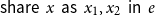 $\mathop{\,\mathsf{share }\,} x \mathop{\,\mathsf{ as }\,} x_1,x_2 \mathop{\,\mathsf{ in }\,} e$
has no effect on the result of a program: it removes the variable x from the scope and introduces two copies
$\mathop{\,\mathsf{share }\,} x \mathop{\,\mathsf{ as }\,} x_1,x_2 \mathop{\,\mathsf{ in }\,} e$
has no effect on the result of a program: it removes the variable x from the scope and introduces two copies
 $x_1$
and
$x_1$
and
 $x_2$
into the scope of e. It is a contraction rule as typically found in linear type systems that provides a controlled mechanism of reference duplication. Variables may be reused indefinitely in AARA, but the duplication of a reference might affect the resource usage of a program; thus,
$x_2$
into the scope of e. It is a contraction rule as typically found in linear type systems that provides a controlled mechanism of reference duplication. Variables may be reused indefinitely in AARA, but the duplication of a reference might affect the resource usage of a program; thus,
 $\mathop{\,\mathsf{share }\,}$
provides an explicit handle for this.
$\mathop{\,\mathsf{share }\,}$
provides an explicit handle for this.
A simple functional language.

Given a function from a functional program, we want to infer an upper bound on its resource usage as a function of its input. We encode this bound through annotations within the type: base types are unannotated, an recursive data type receives one annotation for each kind of its constructors, and a function type receives two annotations:
 \[ A,B ::= \mathbf{1} \mid L^{P}(A) \mid {{A^p} + {B^r}} \mid {{A} \times {B}} | {A}\buildrel {q/q'} \over \longrightarrow{B} \qquad \text{with }p,q,q',r \in \mathbb{Q}^+\]
The intuitive meaning of a function type
 ${A}\buildrel {q/q'} \over \longrightarrow{B}$
is then derived as follows. Given q resources and the resources that are assigned to a function argument v by the annotated type A (see below), the evaluation of the function with argument v does not run out of resources. Moreover, after the evaluation there are q′ resources left in addition to the resources that are assigned to the result of the evaluation by the type B.
${A}\buildrel {q/q'} \over \longrightarrow{B}$
is then derived as follows. Given q resources and the resources that are assigned to a function argument v by the annotated type A (see below), the evaluation of the function with argument v does not run out of resources. Moreover, after the evaluation there are q′ resources left in addition to the resources that are assigned to the result of the evaluation by the type B.
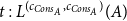
However, let us first encode the above idea into type rules of the form
![]() where
where
 $\Gamma$
is a type context mapping variable names to types, e is a term expression of the simple programming language shown in Figure 1, with A an annotated type as described above and
$\Gamma$
is a type context mapping variable names to types, e is a term expression of the simple programming language shown in Figure 1, with A an annotated type as described above and
 $q,q' \in {\mathbb{Q}_{\geq 0}}$
. We write
$q,q' \in {\mathbb{Q}_{\geq 0}}$
. We write
 $\Gamma_1,\Gamma_2$
for the disjoint union of two type contexts, as usual.
$\Gamma_1,\Gamma_2$
for the disjoint union of two type contexts, as usual.
For simplicity, we will only consider (possibly nested) lists here, but Jost et al. (Reference Jost, Loidl, Hammond, Scaife and Hofmann2009a) show that dealing with arbitrary user-defined recursive data types is straightforward: Each type is annotated with one number for each of its different constructors. This schema would actually entail two annotations for lists, one for the Cons-constructor and one annotation for the Nil-constructor. However, most works omitted the annotation for the Nil-constructor and treated it as constant zero, since in the special case of lists the annotation for the Nil-constructor is entirely redundant. Omitting it thus streamlines the presentation in a paper, but it might be easier to include it in actual implementation to avoid a special case for list types.
Following the previous intuitive description, the rules for variables and constants are straightforward: the amount q of received resources must be greater than the worst-case execution cost c for the respective instruction and the amount q′ of unused resources to be returned:
For bounding heap-space usage, we would choose
 $c_{\text{Var}} = 0$
and
$c_{\text{Var}} = 0$
and
 $c_{\text{Unit}} = 0$
. These cost constants are simply inserted anywhere where costs might be incurred during execution.
$c_{\text{Unit}} = 0$
. These cost constants are simply inserted anywhere where costs might be incurred during execution.
We formulate leave rules like L:Var and L:Unit in a linear style, that is, with contexts that only mention that variables that appear in the terms. We use the following structural weakening rule to obtain more general affine typings. In an implementation, we can simply integrate weakening with the leave rules and use, for instance, an arbitrary context
 $\Gamma$
in the rule L:Unit.
$\Gamma$
in the rule L:Unit.

The following type rule for local definitions shows how resources are threaded into the subexpressions:

For bounding stack-space usage, one might choose
 $c_{\text{Let1}} = 1$
,
$c_{\text{Let1}} = 1$
,
 $c_{\text{Let2}} = 0$
and
$c_{\text{Let2}} = 0$
and
 $c_{\text{Let3}} = -1$
. For worst-case execution time (WCET), all costs constants are non-negative, depending on the actual machine. Heap-space usage is the most simple, with all cost constants in the let rule and most other cost constants being zero. Thus, from now on in this section, we will only consider heap-space usage for brevity and discuss the adaption to other resource later in Section 3.3. Hence, we simply rewrite the type rule for local definitions by:
$c_{\text{Let3}} = -1$
. For worst-case execution time (WCET), all costs constants are non-negative, depending on the actual machine. Heap-space usage is the most simple, with all cost constants in the let rule and most other cost constants being zero. Thus, from now on in this section, we will only consider heap-space usage for brevity and discuss the adaption to other resource later in Section 3.3. Hence, we simply rewrite the type rule for local definitions by:
Note that these type rules assume the decorated q to be numeric constants, but for the inference, the type derivation is constructed assuming fresh names for each of those numeric variables. It is only the validity of the type derivation that depends on the actual numbers, but otherwise no decisions for constructing the type derivation depend on the actual values. So a standard Hindley–Milner–Damas type derivation is performed and all numeric side conditions are simply gathered. Any solution to these numeric constraints then yields a valid type derivation and thus a different bound on resource usage. The solutions are usually obtained by a linear program solver, since the constraints happen to be of the appropriate form.
There are various insignificant choices for the presentation of these rules, for example, unifying some of the numerical variables and making the constraints implicit, as done in many papers to simply shorten the presentation:

Note that these variant type rules now enforce equality between numeric variables instead of certain inequalities. This would deliver exact resource bounds for all possible executions instead of worst-case bounds, which would likely lead to infeasible numeric constraints. Thus, an additional structural type rule L:Relax is then required:
Relying solely on L:Relax for relaxation of numeric constraints has the important benefit of eliminating many boring repetitions from the complicated soundness proof of the annotated type system. Otherwise, resources might be abandoned in many places, as could be seen in L:Let, which would require us to prove three times that it is okay to reduce the resources at hand. For the sake of clarity within this presentation, we will keep to the former style of using explicit numeric constraints within this section.
Likewise, for obtaining concise proofs without too much redundancy, most papers in this field require the program to be automatically converted into a let-normal form (LNF) where sequential composition is only available in let bindings. Other syntactic forms restrict subexpressions to be a variable whenever possible without altering the expressivity of the language. This is similar to but more restrictive than A-normal from Sabry and Felleisen (Reference Sabry and Felleisen1993) where also values may appear in variable positions.
Otherwise, the lengthy proof for case L:Let must be repeated in all other cases of the proof that require proper subexpressions. Since LNF also eases understanding, we follow this conventions here as well. In a practical implementation of AARA, it is easy to drop the requirement for LNF by incorporating the treatment of sequential computations of the let rule in other rules. Alternatively, one can compile unrestricted programs to LNF before the analysis. However, converting a program to LNF might alter its resource usage and additional syntactic forms such as a cost-free let expression must be introduced to ensure that the analysis correctly captures the cost of the source program (Jost et al. Reference Jost, Loidl, Hammond, Scaife and Hofmann2009a).

Cost constants
 $c_{\text{Left}_A}$
and
$c_{\text{Left}_A}$
and
 $c_{\text{Right}_B}$
must be set to the appropriate size of each value;
$c_{\text{Right}_B}$
must be set to the appropriate size of each value;
 $c_{\text{CaseLeft}}$
and
$c_{\text{CaseLeft}}$
and
 $c_{\text{CaseRight}}$
may be zero or set to the respective negative values if the match also deallocates the value from memory, which some papers provided as a variant.
$c_{\text{CaseRight}}$
may be zero or set to the respective negative values if the match also deallocates the value from memory, which some papers provided as a variant.
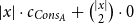
However, in rule L:Left we also see that constructing the value not only requires
 $c_{\text{Left}}$
many resources, but also that p-many free resources are set aside and are no longer available to be used immediately. These p resources become only available again for use upon deconstruction of the value, as can be seen in rule L:MatchSum. In this way, the cost bound of a program is given by its input type: For example, input type
$c_{\text{Left}}$
many resources, but also that p-many free resources are set aside and are no longer available to be used immediately. These p resources become only available again for use upon deconstruction of the value, as can be seen in rule L:MatchSum. In this way, the cost bound of a program is given by its input type: For example, input type
 ${{A^p} + {B^r}}$
encodes that the program requires p resources if given a value constructed with
${{A^p} + {B^r}}$
encodes that the program requires p resources if given a value constructed with
 $\mathop{\,\mathsf{left}\,}$
and r resources for receiving
$\mathop{\,\mathsf{left}\,}$
and r resources for receiving
 $\mathop{\,\mathsf{right}\,}$
as its input. Since types are typically nested, more elaborate cost bounds may be formed.
$\mathop{\,\mathsf{right}\,}$
as its input. Since types are typically nested, more elaborate cost bounds may be formed.
It is important to note that the association of potential different data constructors happens only at the type level. Since it was numerously presumed otherwise, let us be clear: Annotated types are never present at runtime! So when we discuss, for instance, that potential becomes available during a case analysis on a sum type, we merely provide an intuition for understanding the type rules.
The sum of free resources associated with a concrete value through its annotated type is referred to as the potential of this type and value. When we refer to the potential of a type, we mean the function associated with the type that maps a runtime value of this type to the amount of free resources associated with it. The potential function
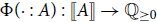 $\Phi(\cdot : A) : \unicode{x27E6} A \unicode{x27E7} \to {\mathbb{Q}_{\geq 0}}$
is defined in Figure 2. The potential function is extended pointwise to environments and contexts by
$\Phi(\cdot : A) : \unicode{x27E6} A \unicode{x27E7} \to {\mathbb{Q}_{\geq 0}}$
is defined in Figure 2. The potential function is extended pointwise to environments and contexts by
 $\Phi(V:\Gamma) = \sum_{x \in V} \Phi\bigl(V(x):\Gamma(x)\bigr)$
. Note that the pair constructor does not have a potential annotation. It could receive an annotation for conformity, but it does not increase the possible resource bounds to be found, since we know already statically that each runtime value of a pair type contains precisely one pair constructor. In contrast, the sum type
$\Phi(V:\Gamma) = \sum_{x \in V} \Phi\bigl(V(x):\Gamma(x)\bigr)$
. Note that the pair constructor does not have a potential annotation. It could receive an annotation for conformity, but it does not increase the possible resource bounds to be found, since we know already statically that each runtime value of a pair type contains precisely one pair constructor. In contrast, the sum type
 ${{A} + {B}}$
requires two resource annotations, one for the Left-constructor and one annotation for the Right-constructor. The important difference being that given a runtime value of this type, we do not know in advance which one of the two constructors will be contained.
${{A} + {B}}$
requires two resource annotations, one for the Left-constructor and one annotation for the Right-constructor. The important difference being that given a runtime value of this type, we do not know in advance which one of the two constructors will be contained.
Potential associated with value v of annotated type A. Note that value v exists at runtime only, while the annotated type A exists at compile time only.
The figure also shows that the potential of a list having length n and type
 $L^{P}(A)$
is
$L^{P}(A)$
is
 $n \cdot p$
, plus the potential contained in elements of the list. The Nil-constructor does not have a potential annotation because a list data structure contains precisely one Nil-constructor. Like for pairs, this allows its potential to be equivalently shifted outwards to the enclosing type or the top-level, if there is no enclosing type around the list.
$n \cdot p$
, plus the potential contained in elements of the list. The Nil-constructor does not have a potential annotation because a list data structure contains precisely one Nil-constructor. Like for pairs, this allows its potential to be equivalently shifted outwards to the enclosing type or the top-level, if there is no enclosing type around the list.
The according typing rules are

A consequence of associating free resources with values through annotated types is that referencing values more than once could lead to an unsound duplication of potential. This is prevented by an explicit contraction rule, which governs how associated resources are distributed between aliased references, thus becoming an affine type system according to Walker (Reference Walker2002). Aliasing is thus not all problematic for the formulation of AARA, since potential is based per-reference anyway.

The contraction rule L:Share relies on the sharing relation
linearly distributing potential between two annotated types, that is, for all values v the inequality
 $\Phi(v:A) \geq \Phi(v:B) + \Phi(v:C)$
holds whenever
$\Phi(v:A) \geq \Phi(v:B) + \Phi(v:C)$
holds whenever
is true. Note that variables that have types without potential may be freely duplicated using the explicit form for sharing.

The two remaining typing rules for function application and abstraction simply track the constant part of the resource cost for evaluating a functions body, the input dependent part being automatically tracked through the annotated argument and result types.

The restriction of pointwise sharing of all types within the context to themselves by
is a simple way to prevent closures from capturing potential, which we will comment upon this in Section 4 and discuss further alternatives there. In a nutshell, this is necessary since we allow unrestricted sharing of functions. If a closure would capture potential, then two uses of that closure would lead to a duplication of the captured potential. Technically, the judgment
forces all resource annotations in the context
 $\Gamma$
to be zero.
$\Gamma$
to be zero.
3.2 Program example: Append
Consider as an example the following definition of a functionFootnote 2 that concatenates two lists:
Let us first consider the expected result intuitively: It is fairly easy to see that function
 ${append}$
constructs precisely one new
${append}$
constructs precisely one new
 ${{\mathop{\,\mathsf{cons}\,}}(,)}$
node for each
${{\mathop{\,\mathsf{cons}\,}}(,)}$
node for each
 ${{\mathop{\,\mathsf{cons}\,}}(,)}$
node contained within its first argument, so a simple heap-space execution cost might expected to be to size of a
${{\mathop{\,\mathsf{cons}\,}}(,)}$
node contained within its first argument, so a simple heap-space execution cost might expected to be to size of a
 ${{\mathop{\,\mathsf{cons}\,}}(,)}$
node times the length of the first argument. We will now show how the analysis concludes this as well.
${{\mathop{\,\mathsf{cons}\,}}(,)}$
node times the length of the first argument. We will now show how the analysis concludes this as well.
Annotating the type with fresh resource variable yields
 ${{{L^{P}(A)} \times {L^{r}(A)}}}\buildrel {q/q'} \over \longrightarrow{L^{s}(A)}$
. The type rules of AARA then construct the cost constraints by starting with q resources, as detailed by the annotation of the function arrow. The resource-annotated type together with the set of constraints can be seen as the most general type. Another point of view would be to consider the constraints to be a description of a set of possible concrete numeric potential annotations.
${{{L^{P}(A)} \times {L^{r}(A)}}}\buildrel {q/q'} \over \longrightarrow{L^{s}(A)}$
. The type rules of AARA then construct the cost constraints by starting with q resources, as detailed by the annotation of the function arrow. The resource-annotated type together with the set of constraints can be seen as the most general type. Another point of view would be to consider the constraints to be a description of a set of possible concrete numeric potential annotations.
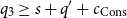
Since the outermost term is a case distinction, type rule L:MatchList applies. The Nil-branch being a simple variable, we obtain, in the terms of type rule L:MatchList, the constraint
 $q = q' + c_{Nil} + c_{CaseNil}$
from rule L:Var. However, we also note that the types
$q = q' + c_{Nil} + c_{CaseNil}$
from rule L:Var. However, we also note that the types
 $L^{r}(A)$
and
$L^{r}(A)$
and
 $L^{s}(A)$
must be identical, so we note the constraint
$L^{s}(A)$
must be identical, so we note the constraint
 $r=s$
, as well, for which most works use an explicit subtyping mechanism omitted here.
$r=s$
, as well, for which most works use an explicit subtyping mechanism omitted here.
For the Cons-branch, the constraint
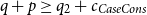 $q + p \geq q_2 + c_{CaseCons}$
shows that from the initial amount of resources q, we must pay the cost for the case distinction and gain the potential associated with one node of the first input list p. Note that the overall potential remains unchanged, since the reference x is no longer available within the typing context; instead, we have the new references h and t. The rule L:MatchList mandates the typings
$q + p \geq q_2 + c_{CaseCons}$
shows that from the initial amount of resources q, we must pay the cost for the case distinction and gain the potential associated with one node of the first input list p. Note that the overall potential remains unchanged, since the reference x is no longer available within the typing context; instead, we have the new references h and t. The rule L:MatchList mandates the typings
 $h:A$
and
$h:A$
and
 $t:L^{P}(A)$
. In this way, it is ensured the potential assigned by p to each element in x and that potential carried by the elements is not duplicated nor lost.Footnote 3
$t:L^{P}(A)$
. In this way, it is ensured the potential assigned by p to each element in x and that potential carried by the elements is not duplicated nor lost.Footnote 3
The subsequent application of L:Let threads these resources to the function application and we obtain the constraints
 $q_2 \geq q + c_{\text{App}}$
and
$q_2 \geq q + c_{\text{App}}$
and
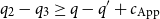 $q_2 - q_3 \geq q - q' + c_{\text{App}}$
with
$q_2 - q_3 \geq q - q' + c_{\text{App}}$
with
 $q_3$
being the amount of resources being supplied to the body of the let expression. The body of the let expression is typed by L:Cons and we obtain
$q_3$
being the amount of resources being supplied to the body of the let expression. The body of the let expression is typed by L:Cons and we obtain
 $q_3 \geq s + q' + c_{\text{Cons}}$
. Gathering and simplifying these constraints, we obtain:
$q_3 \geq s + q' + c_{\text{Cons}}$
. Gathering and simplifying these constraints, we obtain:
 \begin{align*} q - c_{CaseNil} &= q' + c_{Nil} & p - c_{CaseCons} &\geq c_{App} & \\ r &=s & p - c_{CaseCons} &\geq c_{App} + c_{Cons_A} + s &\end{align*}
For heap-space usage, it is reasonable to set all occurring cost constants to zero, except for
 $c_{Cons_A}$
which denotes the cost for allocating a list node for a list of type A. Simplifying the constraints further, we thus inferred the following type for any
$c_{Cons_A}$
which denotes the cost for allocating a list node for a list of type A. Simplifying the constraints further, we thus inferred the following type for any
 $p, q \in {\mathbb{Q}_{\geq 0}}$
:
$p, q \in {\mathbb{Q}_{\geq 0}}$
:
 \[{append}: {{{L^{c_{Cons_A}+p}(A)} \times {L^{P}(A)}}}\buildrel {q/q} \over \longrightarrow{L^{P}(A)}\]
which expresses that the heap-space cost for applying append is precisely
 $n \cdot c_{Cons_A}$
, where n is the length of the first argument list, thus providing a tight upper bound.
$n \cdot c_{Cons_A}$
, where n is the length of the first argument list, thus providing a tight upper bound.
Nested Recursive Data Types and Linear Resource Bounds
Note that the presented method for linear resource bounds already entails the inference of bounds for functions dealing with arbitrarily nested data structures.
For example, given a function that takes a list of lists of type unit as its input, the first paper (Hofmann and Jost Reference Hofmann and Jost2003) could infer a bound of the form
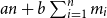 $an + b\sum_{i=1}^{n}m_i$
with
$an + b\sum_{i=1}^{n}m_i$
with
 $a, b \in \mathbb{Q}^{+}$
and
$a, b \in \mathbb{Q}^{+}$
and
 $n, m_i \in \mathbb{N}$
, where n is the length of the outer list and
$n, m_i \in \mathbb{N}$
, where n is the length of the outer list and
 $m_i$
is the length of each inner list for
$m_i$
is the length of each inner list for
 $i\in{1,\dots,n}$
. Such an upper bound would be expressed by the annotated input type
$i\in{1,\dots,n}$
. Such an upper bound would be expressed by the annotated input type
 $L^{a}({L^{b}({unit})})$
.
$L^{a}({L^{b}({unit})})$
.
For
 $m = max(m_i)$
we then obtain the upper bound
$m = max(m_i)$
we then obtain the upper bound
 $n \cdot m$
, which might be considered to be a quadratic bound. Likewise, in this way a list of lists of lists would lead to a cubic bound.
$n \cdot m$
, which might be considered to be a quadratic bound. Likewise, in this way a list of lists of lists would lead to a cubic bound.
However, since the early versions of AARA could not yet infer general bounds involving expressions such as
 $n \cdot m_i$
, we consider these versions to deliver linear resource bounds only. See Section 5 for the proper treatment of truly super- and sub-linear bounds.
$n \cdot m_i$
, we consider these versions to deliver linear resource bounds only. See Section 5 for the proper treatment of truly super- and sub-linear bounds.
3.3 Accounting for different resources
Most of the research papers considered in this survey focused on heap-space usage. However, Jost et al. (Reference Jost, Loidl, Hammond, Scaife and Hofmann2009a) showed that it is straightforward to eschew any resource whose cost can be statically bound to each individual instruction by choosing the appropriate cost constants. Note that soundness can be proven independently of these cost constants by proving soundness with respect to a cost-instrumented operational semantics using the same symbolic cost constants. Thereby, the same proof holds for arbitrary resource cost models and one must just verify the cost-instrumented operational semantics match reality.
In addition to the flexibility provided by the cost constants, it is easy to also include a general cost-counting statement
 ${tick}~q$
for explicitly stating costs within the code:
${tick}~q$
for explicitly stating costs within the code:
The tick-statement evaluates to the unit value and in functional code is mostly used by constructs like
 $\mathop{\,\mathsf{let }\,} _ = \mathop{\,\mathsf{tick}\,} q \mathop{\,\mathsf{ in }\,} e$
or so.
$\mathop{\,\mathsf{let }\,} _ = \mathop{\,\mathsf{tick}\,} q \mathop{\,\mathsf{ in }\,} e$
or so.
Considering stack-space usage is straightforward in principle, but the linear bounds of the early research were a practical hindrance. This was addressed by Campbell (Reference Campbell2009) in 2009. However, significant further progress should be expected if the insights of the decade of AARA research that followed after 2009 would be applied to the problems shown by Campbell.
Determining the WCET in actual processor clock cycles is also possible, as shown in detail in Jost et al. (Reference Jost, Loidl, Hammond, Scaife and Hofmann2009a); Jost et al. (Reference Jost, Loidl, Scaife, Hammond, Michaelson and Hofmann2009b). However, this requires one to obtain the WCET for each basic block that might be produced by the binary compiler, since AARA excels at the high level where nested data structures and recursion are abundant. Thus, in the aforementioned works on WCET, the bounds on the basic blocks were established by abstract interpretations methods working on the low-level code. For a simple processor like the Renesas M32C/85, this combined analysis delivered a WCET bound less than 34% above the worst measured runtime in the considered scenarios.
Another application area of AARA gas analysis is smart contracts (Das et al. Reference Das, Balzer, Hoffmann, Pfenning and Santurkar2021; Das and Qadeer Reference Das, Qadeer and Sighireanu2020). Gas is a high-level resource that used to model the execution cost of a smart contract. Gas is important to prevent denial-of-service attacks on blockchains. Commonly, users of smart contracts are required to pay for the gas consumption of a transaction in advance without knowing the memory state of the contract. As a result, statically predicting the gas cost is desirable. Technically, gas can treated like execution time in AARA.
Another resource of interest is energy. We believe that an analysis of the energy consumption of a program with AARA is possible but we are not aware of any works in this space. A challenge could be the need to not only model the energy cost of the processor but also of other devices, such as radios or sensors, that are used by a program.
3.4 Soundness
The main result of many AARA papers is the proof of soundness for the annotated type system, which formally guarantees that the resource bounds are indeed an upper bound on resource usage with respect to a formal cost-instrumented operational semantics.
Usually a big-step semantics is used, as it fits the type rules best. Since big-step semantics only deal with terminating computations, an additional big-step semantics for partial evaluation can be provided. This also allows to prove that even the resource usage of failing or non-terminating programs respects the inferred resource bounds (Hoffmann and Hofmann Reference Hoffmann and Hofmann2010a; Jost 2012). However, the semantics for partial evaluations are usually just a straightforward variant of the ordinary big-step semantics, so we do not repeat this common simple solution to the problem of big-step semantics in this survey paper.
There are several ways to define the cost-instrumented operational semantics. Here, we write
 \[V \vdash e {\Downarrow {v}} \mid (p,p')\]
to denote that expression e evaluates in environment V to value v, with p being the minimal amount of resources needed for the evaluation, and p′ the amount of unused resources being available after the evaluation.
The soundness proof usually proceeds by induction on the lexicographically ordered lengths of the formal evaluation and the typing derivation. The proof is primarily divided by a case distinction on the syntactic construct at the current end of the type derivation, but due to structural type rules and the lengthening of the typing derivation in case of function calls or thunks, the lexicographic ordering with a formal evaluation is usually required. A typical formulation of the soundness proof has the following structure:

Type preservation
 $v : A$
must sometimes be proven simultaneously within the main soundness theorem as included above, since resource usage becomes an intrinsic property of functions and thunks. Type systems without higher-order types nor laziness typically allow preservation to be proven independently.
$v : A$
must sometimes be proven simultaneously within the main soundness theorem as included above, since resource usage becomes an intrinsic property of functions and thunks. Type systems without higher-order types nor laziness typically allow preservation to be proven independently.
Note that some AARA presentations separated the evaluation environment
 $V = (S,H)$
into stack S and heap H (Hofmann and Jost Reference Hofmann and Jost2003; Jost et al. Reference Jost, Loidl, Hammond, Scaife and Hofmann2009a). This facilitates motivating the cost annotation for stack and heap space usage but is not mathematically relevant since the assigned cost and computed values are identical.
$V = (S,H)$
into stack S and heap H (Hofmann and Jost Reference Hofmann and Jost2003; Jost et al. Reference Jost, Loidl, Hammond, Scaife and Hofmann2009a). This facilitates motivating the cost annotation for stack and heap space usage but is not mathematically relevant since the assigned cost and computed values are identical.
Alternative Cost-Instrumented Operational Semantics
The above depicted cost-instrumented big-step semantics deliver the minimal resources required for evaluation; this allows for a concise theorem statement at the expense of requiring more care within the proof itself.
Alternatively, the big-step operational semantics could be instrumented with a simple counter that just increases and decreases with each rule application, according to the cost constants. We write
to denote that expression e evaluates in environment V to value v, with m resources being initially available and and m′ resources being unused after the evaluation. The derivation in this semantics simply fails whenever the amount of available resource would become negative. So if m is chosen too small, then no derivation is possible within these cost-instrumented semantics.
Usually, one can prove that for all
 $n \geq m$
that there exists an n′ with
$n \geq m$
that there exists an n′ with
 $n' \geq m' + (n - m)$
such that
$n' \geq m' + (n - m)$
such that
![]() is possible, that is, excess resources are harmless and preserved.
is possible, that is, excess resources are harmless and preserved.
This latter version of cost-instrumented semantics was especially used in earlier AARA papers, since it simplifies the proof at the cost of a more complicated statement of the soundness theorem, which then becomes:

Note the inverted inequalities involving the resource bounds.
The value r allows threading of unused excess resources to subsequent subexpressions; programs in LNF then require this for local
 $\mathop{\,\mathsf{let}\,}$
-definitions only. Note that an explicit r can be avoided by referring to differences, similarly to the type rule L:Relax depicted above.
$\mathop{\,\mathsf{let}\,}$
-definitions only. Note that an explicit r can be avoided by referring to differences, similarly to the type rule L:Relax depicted above.
The theorem sketched above intuitively says that an evaluation with restricted resources cannot fail due to a lack of resources if the amount of available resources exceeds the upper bound indicated by the annotated types.
3.5 Manual amortized analysis
The similarity of the program analysis outlined above and the manual amortized analysis technique by Tarjan (Reference Tarjan1985) was only later pointed out to us by our colleague Olha Shkaravska around 2004.
Tarjan’s amortized analysis basically allows any kind of mathematical potential function that abstracts any program configuration to simple number. However, the onus is on the user to find a suitable abstraction so that the proof of the desired program property succeeds.
In contrast, the presented analysis restricts this vast search space to a certain set of functions encoded through the type only in a canonical way. This reduced inference to solving a set of linear inequalities, which by chance had the property to be easily solvable. The research that followed the initial work then pushed hard to enlarge the search space again, while retaining a feasible inference.
An important advantage of AARA over Tarjan’s original amortized analysis is the idea to assign potential per reference to a data structure. While the manual amortized analysis generally breaks in the presence of persistent data structures (Okasaki Reference Okasaki1998), the potential per typed reference is the key to the success of AARA in a functional setting.
4. Higher-Order and Other Extensions
Adapting AARA to a higher-order functional language required several steps, most of which are not directly related to higher-order types. Instead, these features are already beneficial in a first-order setting, albeit arguably less urgently so. We discuss these steps in no particular order.
Resource Parametricity
Consider the heap-space usage of a function
 ${zip} : {{{L^{P}(A)} \times {L^{q}(B)}}}\buildrel {0/0} \over \longrightarrow{L^{r}({{A} \times {B}})}$
that zips a pair of lists into a list of pairs. Assume the cost
${zip} : {{{L^{P}(A)} \times {L^{q}(B)}}}\buildrel {0/0} \over \longrightarrow{L^{r}({{A} \times {B}})}$
that zips a pair of lists into a list of pairs. Assume the cost
 $c_{\text{pair}}=2$
for constructing a list node of the output, including a pair constructor. It is then easy to see that the cost constraints are
$c_{\text{pair}}=2$
for constructing a list node of the output, including a pair constructor. It is then easy to see that the cost constraints are
 $p + q \geq r + c_{\text{pair}}$
, and indeed the AARA will infer a more elaborate LP which could then be simplified to this equation.
$p + q \geq r + c_{\text{pair}}$
, and indeed the AARA will infer a more elaborate LP which could then be simplified to this equation.
The problem then arises by our insistence to have a single solution to a single LP, which prevents simultaneous calls with the otherwise valid types
 ${zip} : {{{L^{3}(A)} \times {L^{0}(B)}}}\buildrel {0/0} \over \longrightarrow{L^{1}({{{A} \times {B}}})}$
and
${zip} : {{{L^{3}(A)} \times {L^{0}(B)}}}\buildrel {0/0} \over \longrightarrow{L^{1}({{{A} \times {B}}})}$
and
 ${zip} : {{{L^{0}(A)} \times {L^{3}(B)}}}\buildrel {0/0} \over \longrightarrow{L^{1}({{{A} \times {B}}})}$
. The solution presented in Jost et al. (Reference Jost, Hammond, Loidl and Hofmann2010), Jost (2012) is an annotated function type that also stores a set of constraints, as well as the set of bound constraint variables. Note that free constraint variables must allowed to be retained as well. Upon each function application, this set of constraints is simply copied into the actual constraints for the programs, with the bound constraint variables being renamed.
${zip} : {{{L^{0}(A)} \times {L^{3}(B)}}}\buildrel {0/0} \over \longrightarrow{L^{1}({{{A} \times {B}}})}$
. The solution presented in Jost et al. (Reference Jost, Hammond, Loidl and Hofmann2010), Jost (2012) is an annotated function type that also stores a set of constraints, as well as the set of bound constraint variables. Note that free constraint variables must allowed to be retained as well. Upon each function application, this set of constraints is simply copied into the actual constraints for the programs, with the bound constraint variables being renamed.
Note that this makes the size of the LP exponential in the depth of the call graph, which turned out to be mostly unproblematic in practice.
Mutual Recursion
Mutual recursion can in principle be dealt with easily, since the annotated type of a function featuring numeric variables instead of numeric constant values is created before the examination of the function body. Each application simply refers to these previously determined annotated types, recursive or otherwise. This requires the annotations to become first-class elements to be manipulated during the inference, as well as explicitly passing sets of constraints at the time of function application.
Polymorphism
Dealing with polymorphic functions requires to defer a part of inference: a function’s constraint set then contains symbolic constraints that are instantiated upon function application, given the appropriate types. These symbolic constraints simply express the number of times an argument must be shared to the various references occurring within a function’s body.
Currying and Closures with Potential
Type rule L:Fun in Section 3 contains the premise
![]() that effectively disallows potential to be captured in closures. Any potential captured within a function closure would be available for each application, leading to an unsound duplication of potential. Restricting potential to zero is one easy way out of this problem, another would be use-once (or use-n-times) function types. Both of these strategies are not in opposition but can be combined in one type system, as demonstrated by Rajani et al. (Reference Rajani, Gaboardi, Garg and Hoffmann2021).
that effectively disallows potential to be captured in closures. Any potential captured within a function closure would be available for each application, leading to an unsound duplication of potential. Restricting potential to zero is one easy way out of this problem, another would be use-once (or use-n-times) function types. Both of these strategies are not in opposition but can be combined in one type system, as demonstrated by Rajani et al. (Reference Rajani, Gaboardi, Garg and Hoffmann2021).
Note that restricting potential of closures for thunks to zero is not an acceptable solution, but thunks being use-once functions resolve this problem automatically, albeit making soundness much more harder to prove, see Section 6.
An important consequence of restricting closure potential to zero is that only the last function argument is allowed to yield any potential, which in turn gives AARA a strong preference for fully uncurried functions, which do not suffer from this limitation at all.
Beyond Worst-Case Bounds
It is also possible to use AARA to derive lower bounds on the best case resource usage and to precisely characterize the resource usage of programs (Ngo et al. Reference Ngo, Dehesa-Azuara, Fredrikson and Hoffmann2017). For a precise characterization, we simply remove the weakening rules and require that all potential needs to be consumed in every branch. Such precise characterizations are interesting in the context of software security, where we would like to show the absence of side channels based on resource usage.
For lower bounds, we also remove weakening but allow to create potential. However, we require that all potential needs to be used to pay for cost at some point. Intuitively, the goal is to spend as much potential as possible to justify a tighter lower bound.
The original AARA corresponds to an affine treatment, the precise analysis to a linear treatment, and the lower-bound analysis to a relevant treatment of potential.
5. Non-Linear Potential Functions
AARA, as introduced by Hofmann and Jost (Reference Hofmann and Jost2003), was well received by the research community. However, the correlation of the technique with linear potential functions, and thus linear bounds, has often been cited as its main limitation.Footnote 4 Indeed, the association of a constant potential with each element of a data structure seemed to be the focal point that enabled local and intuitive typing rules as well as the type and bound inference via off-the-shelf LP solvers. A naive extension to non-linear potential functions would require non-linear constraint solving an additional expressivity in the type system as offered by dependent types (Martin-Löf Reference Martin-Löf1984) or refinement types (Freeman and Pfenning Reference Freeman, Pfenning and Wise1991). An AARA in such a setting would not share many of the characteristics of the original linear version and it is not clear if the potential method would provide advantages (Radiček et al. 2017).
Maybe unexpectedly, even to the surprise of Hofmann and Jost, it could be demonstrated that AARA can be extended to non-linear potential functions while preserving all benefits of the technique, including local typing rules and reducing bound inference to linear constraint solving. The first such extension uses univariate polynomial potential functions and has been developed by Hoffmann and Hofmann in 2009 (Hoffmann and Hofmann Reference Hoffmann and Hofmann2010b). Subsequently, extensions to multivariate polynomial potential functions (Hoffmann et al. Reference Hoffmann, Aehlig and Hofmann2011) and exponential potential functions (Kahn and Hoffmann Reference Kahn and Hoffmann2020) have been developed. Recently, an AARA with logarithmic potential has been proposed (Hofmann et al. Reference Hofmann, Leutgeb, Obwaller, Moser and Zuleger2021; Hofmann and Moser Reference Hofmann and Moser2018).
The extensions to polynomial potential and exponential potential are conservative over the original linear system. However, while potential in linear AARA can be parametric in the values of general recursive types (Jost et al. Reference Jost, Loidl, Hammond, Scaife and Hofmann2009a; Jost et al. Reference Jost, Hammond, Loidl and Hofmann2010), polynomial potential has been introduced for a particular form of inductive typesFootnote 5 only (Hoffmann et al. Reference Hoffmann, Das and Weng2017) and exponential potential has only been developed for lists thus far. Polynomial potential can be a function of either the size or the height of data structures (Hoffmann Reference Hoffmann2011). In this section, we focus on lists for which the notions of height and size coincide.
5.1 Univariate polynomial potential
Univariate polynomial AARA (Hoffmann and Hofmann Reference Hoffmann and Hofmann2010b) is a conservative extension of linear AARA (Hofmann and Jost Reference Hofmann and Jost2003). The only type rules that differ between the systems are the ones for constructing and destructing data structures. In the following, we explain the idea for lists. It can be extended to other tree-like inductive types.
Resource Annotations
In linear AARA, list types are annotated with a single non-negative rational number q that defines the potential function
 $q\cdot n$
, where n is the length of the list. In univariate polynomial AARA, we use potential functions that are non-negative linear combinations of binomial coefficients
$q\cdot n$
, where n is the length of the list. In univariate polynomial AARA, we use potential functions that are non-negative linear combinations of binomial coefficients
 $\binom{n}{k}$
, where k is a natural number and n is the length of the list. Consequently, a resource annotation for lists is a vector
$\binom{n}{k}$
, where k is a natural number and n is the length of the list. Consequently, a resource annotation for lists is a vector
 $\vec q = (q_1,\ldots,q_k) \in ({\mathbb{Q}_{\geq 0}})^k$
of non-negative rational numbers and list types have the form
$\vec q = (q_1,\ldots,q_k) \in ({\mathbb{Q}_{\geq 0}})^k$
of non-negative rational numbers and list types have the form
 $L^{\vec q}(A)$
.
$L^{\vec q}(A)$
.
One intuition for the resource annotations is as follows: The annotation
 $\vec q$
assigns the potential
$\vec q$
assigns the potential
 $q_1$
to every element of the data structures, the potential
$q_1$
to every element of the data structures, the potential
 $q_2$
to every element of every proper suffix (sublist or subtree, respectively) of the data structure,
$q_2$
to every element of every proper suffix (sublist or subtree, respectively) of the data structure,
 $q_3$
to the elements of the suffixes of the suffixes, etc.
$q_3$
to the elements of the suffixes of the suffixes, etc.
The choice of binomial coefficients is beneficial compared to the standard basis (n,
 $n^2$
,
$n^2$
,
 $\ldots$
) if we ensure that potential functions are non-negative by only allowing non-negative potential annotations. With non-negative coefficients, functions like
$\ldots$
) if we ensure that potential functions are non-negative by only allowing non-negative potential annotations. With non-negative coefficients, functions like
 $\binom{n}{2}$
cannot be expressed in the standard basis. Binomial coefficients with non-negative coefficients are also a canonical choice since they are the largest class of inherently non-negative polynomials (Hoffmann et al. Reference Hoffmann, Aehlig and Hofmann2011).
$\binom{n}{2}$
cannot be expressed in the standard basis. Binomial coefficients with non-negative coefficients are also a canonical choice since they are the largest class of inherently non-negative polynomials (Hoffmann et al. Reference Hoffmann, Aehlig and Hofmann2011).
The Potential of Lists
Let us now consider the construction or destruction of non-empty lists. For linear potential annotations, we can simply assign potential to the tail using the same annotation as on the original list. This would however lead to a substantial loss of potential in the polynomial case. For this reason, we use an additive shift operation to assign potential to sublists. The additive shift of
 $\vec q = (q_1,\ldots,q_k)$
is
$\vec q = (q_1,\ldots,q_k)$
is
 \[\lhd(\vec q) = (q_1 + q_2, q_2 + q_3, \ldots, q_{k-1} + q_{k},q_k)\; .\]
The definition of potential
 $\Phi(v:A)$
of a value v of type A is extended as follows:
$\Phi(v:A)$
of a value v of type A is extended as follows:
 \[\begin{array}{lll} \Phi([\,] : L^{\vec q}(A) ) &=& 0 \\ \Phi({{v_1}\mathop{::}{v_2}} : L^{\vec q}(A) ) &=& \Phi(v_1 : A) + q_1 + \Phi(v_2 : L^{\lhd{\vec q}}(A)\end{array}\]
The potential of a list can be written as a non-negative linear combination of binomial coefficients. If we define
 \[\phi(n,\vec q) = \sum_{i=1}^{k} \binom{n}{i} q_i\]
then we can prove the following lemma.
Lemma 1. Let
 $\ell = [v_1 \ldots, v_n]$
be a list whose elements are values of type A. Then
$\ell = [v_1 \ldots, v_n]$
be a list whose elements are values of type A. Then
 \[\Phi(\ell{:}L^{\vec q}(A)) = \phi(n,\vec q) + \sum_{i=1}^{n} \Phi(v_i{:}A)\; . \]
The use of binomial coefficients instead of powers of variables is not theoretically appealing but has also several practical advantages. In particular, the identity
 \[\sum_{i=1,\ldots,k} q_i\binom{n+1}{i} = q_1+ \sum_{i=1,\ldots,k-1} q_{i+1} \binom{n}{i} + \sum_{i=1,\ldots,k}q_i\binom{n}{i}\]
gives rise to a local typing rule for
 $\mathop{\,\mathsf{cons}\,}$
and pattern matching, which naturally allows the typing of both recursive calls and other calls to subordinate functions in branches of a pattern match.
$\mathop{\,\mathsf{cons}\,}$
and pattern matching, which naturally allows the typing of both recursive calls and other calls to subordinate functions in branches of a pattern match.
Typing Rules
Like for linear potential functions, the type rules define a judgment of the form
The rules of linear AARA remain unchanged except for the rules for the introduction and elimination of inductive types. Below are the rules for lists. To focus on the novel aspects, we assume that the cost constants are zero. They can be added like in the linear case.

The rule U:Nil requires no additional constant potential and an empty context. It is sound to attach any potential annotation
 $\vec p$
to the empty list since the resulting potential is always zero. The rule U:Cons reflects the fact that we have to cover the potential that is assigned to the new list of type
$\vec p$
to the empty list since the resulting potential is always zero. The rule U:Cons reflects the fact that we have to cover the potential that is assigned to the new list of type
 $L^{\vec p}({\vec A})$
. We do so by requiring
$L^{\vec p}({\vec A})$
. We do so by requiring
 $x_2$
to have the type
$x_2$
to have the type
 $L^{\lhd(\vec p)}(A)$
and to have
$L^{\lhd(\vec p)}(A)$
and to have
 $p_1$
resource units available. The rule U:MatL accounts for the fact that either
$p_1$
resource units available. The rule U:MatL accounts for the fact that either
 $e_0$
or
$e_0$
or
 $e_1$
is evaluated. The cons case is inverse to the rule U:Cons and uses the potential associated with a list:
$e_1$
is evaluated. The cons case is inverse to the rule U:Cons and uses the potential associated with a list:
 $p_1$
resource units become available as constant potential and the tail of the list is annotated with
$p_1$
resource units become available as constant potential and the tail of the list is annotated with
 $\lhd(\vec p)$
.
$\lhd(\vec p)$
.
Example: Alltails
Recall the function append from Section 3.2 and consider again the resource metric for heap space in which all costs are 0 except for
 $c_{Cons_A}$
, which is the cost of list cons.
$c_{Cons_A}$
, which is the cost of list cons.
With this metric, heap-space cost for evaluating append(x,y) is
 $|x| \cdot c_{Cons_A}$
. This exact bound is reflected by the following typing:
$|x| \cdot c_{Cons_A}$
. This exact bound is reflected by the following typing:
 \[{append}: {{{L^{(c_{Cons_A},0)}(A)} \times {L^{(0,0)}(A)}}}\buildrel {0/0} \over \longrightarrow{L^{(0,0)}(A)}\]
The typing is similar to the one that is discussed in Section 3.2. However, we are considering the special case in which resulting potential is zero as indicated by the annotations on the result type. Moreover, we have added quadratic potential annotations. For instance, the annotated type
 $L^{(c_{Cons_A},0)}(A)$
on the first argument x of append assigns the potential
$L^{(c_{Cons_A},0)}(A)$
on the first argument x of append assigns the potential
 $|x| \cdot c_{Cons_A} + \binom{|x|}{2} \cdot 0$
. To give the most general type for append with quadratic potential, we need multivariate annotations. More details are discussed in Section 5.2.
$|x| \cdot c_{Cons_A} + \binom{|x|}{2} \cdot 0$
. To give the most general type for append with quadratic potential, we need multivariate annotations. More details are discussed in Section 5.2.
For an example with non-trivial quadratic annotations, consider the following function alltails that creates a list that is a concatenation of all tails, that is, all proper suffixes, of the argument.
With the heap resource metric, the resource consumption of the alltails is
 $\binom{n}{2} \cdot c_{Cons_A}$
, where n is the length of the argument. In the univariate system, this exact bound can be expressed by the following typing:
$\binom{n}{2} \cdot c_{Cons_A}$
, where n is the length of the argument. In the univariate system, this exact bound can be expressed by the following typing:
 \[{alltails}: {L^{(0,c_{Cons_A})}(A)}\buildrel {0/0} \over \longrightarrow{L^{(0,0)}(A)}\]
The key aspect of the type derivation is the treatment of the cons case of the case analysis in the function body. The types of the variables are
 $h:A$
and
$h:A$
and
 $t:L^{(c_{Cons_A},c_{Cons_A})}(A)$
. The annotation
$t:L^{(c_{Cons_A},c_{Cons_A})}(A)$
. The annotation
 $(c_{Cons_A},c_{Cons_A})$
is the result of the additive shift
$(c_{Cons_A},c_{Cons_A})$
is the result of the additive shift
 $\lhd(0,c_{Cons_A})$
. The potential is then shared as
$\lhd(0,c_{Cons_A})$
. The potential is then shared as
 $t_1:L^{(0,c_{Cons_A})}(A)$
to match the argument type (and cover the cost) of the recursive call and
$t_1:L^{(0,c_{Cons_A})}(A)$
to match the argument type (and cover the cost) of the recursive call and
 $t_2:L^{(c_{Cons_A}),0}(A)$
to match the argument type of append.
$t_2:L^{(c_{Cons_A}),0}(A)$
to match the argument type of append.
Note that we assume
![]() , that is, the type A does not carry potential. This is needed because elements of the inner list are copied. In the multivariate system, we can type the function alltails with element types that carry potential.
, that is, the type A does not carry potential. This is needed because elements of the inner list are copied. In the multivariate system, we can type the function alltails with element types that carry potential.
Soundness
The soundness theorem has the same form as for linear AARA. Given the appropriate extensions of sharing and subtyping, the change in the proof is limited to the cases that involve the syntactic forms for lists.
Theorem. Let
![]() and
and
 $V : \Gamma$
. If
$V : \Gamma$
. If
 $V \vdash e {\Downarrow {v}} \mid (p,p')$
for some v and (p, p′) then
$V \vdash e {\Downarrow {v}} \mid (p,p')$
for some v and (p, p′) then
 $\Phi(V : \Gamma) + q \geq p$
and
$\Phi(V : \Gamma) + q \geq p$
and
 $\Phi(V : \Gamma) + q - (\Phi(v:A) + q') \geq p - p'$
.
$\Phi(V : \Gamma) + q - (\Phi(v:A) + q') \geq p - p'$
.
The proof is by induction on the evaluation judgment and an inner induction on the type judgment. The inner induction is needed because of the structural rules.
Type Inference and Resource-Polymorphic Recursion
The basis of the type inference for the univariate polynomial system is the type inference algorithm for the linear system, which reduces the inference of potential functions to LP. A further challenge for the inference of polynomial bounds is the need to deal with resource-polymorphic recursion, which is required to type many functions that are not tail recursive and have a superlinear cost.
It is a hard problem to infer general resource-polymorphic types, even for the original linear system. A pragmatic approach to resource-polymorphic recursion that works well and efficiently in practice is to apply so-called cost-free typings that only transfer potential from arguments to results. More details can be found in the literature (Hoffmann and Hofmann Reference Hoffmann and Hofmann2010a).
5.2 Multivariate polynomial potential
Linear AARA is compositional in the sense that the typeability of two functions f and g is often indicative of the typeability of the function composition
 $f \circ g$
. However, this is not the case to the same extent for univariate polynomial AARA. Consider for instance the function append :
$f \circ g$
. However, this is not the case to the same extent for univariate polynomial AARA. Consider for instance the function append :
 $L({\mathbf{1}}) \times L({\mathbf{1}}) \to L({\mathbf{1}})$
for integer lists and the sorting function quicksort :
$L({\mathbf{1}}) \times L({\mathbf{1}}) \to L({\mathbf{1}})$
for integer lists and the sorting function quicksort :
 $L({\mathbf{1}}) \to L({\mathbf{1}})$
. Using univariate AARA, we can derive a linear bound like
$L({\mathbf{1}}) \to L({\mathbf{1}})$
. Using univariate AARA, we can derive a linear bound like
 $n_1$
for append and a quadratic bound like
$n_1$
for append and a quadratic bound like
 $n^2$
for quicksort. Here, we assume that the lengths of the two arguments of append are
$n^2$
for quicksort. Here, we assume that the lengths of the two arguments of append are
 $n_1$
and
$n_1$
and
 $n_2$
, respectively, and that the length of the argument of quicksort is n. Now consider the function
$n_2$
, respectively, and that the length of the argument of quicksort is n. Now consider the function
 $$fun app - qs (x,y) = quicksort(append(x,y)).$$
Assuming the bounds
 $n_1$
and
$n_1$
and
 $n^2$
, a tight bound for the function app-qs is
$n^2$
, a tight bound for the function app-qs is
 $n_1^2 + 2 n_1n_2 + n_2^2 + n_1$
. This bound is not expressible in the univariate system, but one might expect that a looser bound like
$n_1^2 + 2 n_1n_2 + n_2^2 + n_1$
. This bound is not expressible in the univariate system, but one might expect that a looser bound like
 $4n_1^2 + 4n_2^2 + n_1$
is derivable. However, the function app-qs is not typeable in univariate AARA since univariate potential functions cannot express suitable invariants in the type derivation of append. The desire to improve compositionality of polynomial AARA and to express more precise bounds leads to the development of multivariate polynomial AARA in 2010 (Hoffmann et al. Reference Hoffmann, Aehlig and Hofmann2011).
$4n_1^2 + 4n_2^2 + n_1$
is derivable. However, the function app-qs is not typeable in univariate AARA since univariate potential functions cannot express suitable invariants in the type derivation of append. The desire to improve compositionality of polynomial AARA and to express more precise bounds leads to the development of multivariate polynomial AARA in 2010 (Hoffmann et al. Reference Hoffmann, Aehlig and Hofmann2011).
Multivariate AARA is an extension of univariate AARA. It preserves the principles of the univariate system while expanding the set of potential functions so as to express dependencies between different data structures. The term multivariate refers to the use of multivariate monomials like
 $n_1 n_2$
as base functions. They enable us to derive the aforementioned bound
$n_1 n_2$
as base functions. They enable us to derive the aforementioned bound
 $n_1^2 + 2 n_1n_2 + n_2^2 + n_1$
for the function app-qs.
$n_1^2 + 2 n_1n_2 + n_2^2 + n_1$
for the function app-qs.
Resource Annotations and Base Polynomials
Other than in univariate, potential annotations are now global and there is exactly one annotation per type. More formally, we can write data types that do not contain function arrows as pairs
 ${{\langle {\tau},{Q} \rangle}}$
so that τ is a standard type like
${{\langle {\tau},{Q} \rangle}}$
so that τ is a standard type like
 $L({L({\mathbf{1}})})$
and the potential annotation
$L({L({\mathbf{1}})})$
and the potential annotation
 $Q = (q_i)_{i \in I(\tau)}$
is a family of non-negative rational numbers
$Q = (q_i)_{i \in I(\tau)}$
is a family of non-negative rational numbers
 $q_i \in {\mathbb{Q}_{\geq 0}}$
.
$q_i \in {\mathbb{Q}_{\geq 0}}$
.
The (possible infinite) index set I(τ) contains an index i for every base polynomial
 $p_i$
for that type. In a well-formed potential annotation only finitely many
$p_i$
for that type. In a well-formed potential annotation only finitely many
 $q_i$
are larger than 0. For example, we have
$q_i$
are larger than 0. For example, we have
 $I(L({\mathbf{1}})) = \mathbb{N}$
and
$I(L({\mathbf{1}})) = \mathbb{N}$
and
 $p_i(n) = \binom{n}{i}$
. The potential defined by an annotation Q is then
$p_i(n) = \binom{n}{i}$
. The potential defined by an annotation Q is then
 $\sum_{i \in I(L({\mathbf{1}}))} q_i p_i$
. Note that the constant potential (
$\sum_{i \in I(L({\mathbf{1}}))} q_i p_i$
. Note that the constant potential (
 $\binom{n}{0}$
) is also included in the global annotation. As another example, we have
$\binom{n}{0}$
) is also included in the global annotation. As another example, we have
 $I(L({\mathbf{1}}) \times L({\mathbf{1}})) = \mathbb{N} \times \mathbb{N}$
and
$I(L({\mathbf{1}}) \times L({\mathbf{1}})) = \mathbb{N} \times \mathbb{N}$
and
 $p_{(i,j)}(n,m) = \binom{n}{i}\binom{m}{j}$
.
$p_{(i,j)}(n,m) = \binom{n}{i}\binom{m}{j}$
.
The Potential of Lists and Pairs
In general, the base polynomials
 $\mathcal{B}{\tau}$
are inductively defined for inductive data structures and can, for example, take into account the number of certain constructors used in that data structure. For lists and pairs, the inductive definition looks as follows.
$\mathcal{B}{\tau}$
are inductively defined for inductive data structures and can, for example, take into account the number of certain constructors used in that data structure. For lists and pairs, the inductive definition looks as follows.
 \begin{eqnarray*} \mathcal{B}(\mathrm{unit}) &=& \{ \lambda (v) \, 1 \} \\ \mathcal{B}({{\tau_1} \times {\tau_2}}) &=& \{ \lambda ( {\langle {v_1},{v_2} \rangle} ) \; p_1(v_1) {\cdot} p_2(v_2) \mid p_i \in \mathcal{B}(\tau_i) \} \\ \mathcal{B}(L(\tau)) &=& \big\{ \lambda ([v_1,\ldots,v_n]) \; \sum_{1 \leq j_1 < \cdots < j_k \leq n} \, \prod_{1 \leq i \leq k} p_i(v_{j_i}) \mid k \in \mathbb{N}, p_i \in \mathcal{B}(\tau) \big\}\end{eqnarray*}
The last part of the definition is based on the observation that typical polynomial computations operating on a list
 $v = [a_1, \ldots, a_n]$
consist of operations that are executed for every k-tuple
$v = [a_1, \ldots, a_n]$
consist of operations that are executed for every k-tuple
 $(a_{i_1},\ldots,a_{i_k})$
with
$(a_{i_1},\ldots,a_{i_k})$
with
 $1 \leq i_1 < \cdots < i_k \leq n$
. The simplest examples are linear map operations that perform some operation for every
$1 \leq i_1 < \cdots < i_k \leq n$
. The simplest examples are linear map operations that perform some operation for every
 $a_i$
. Another example are common sorting algorithms that perform comparisons for every pair
$a_i$
. Another example are common sorting algorithms that perform comparisons for every pair
 $(a_i,a_j)$
with
$(a_i,a_j)$
with
 $1 \leq i < j \leq n$
in the worst case.
$1 \leq i < j \leq n$
in the worst case.
The potential functions are non-negative linear combination of base polynomials. Consequently, potential annotation consists of coefficients of base polynomials. To assign a unique name to each base polynomial, define the index set
 $\mathcal{I}(\tau)$
to denote resource polynomials for a given type τ.
$\mathcal{I}(\tau)$
to denote resource polynomials for a given type τ.
 \begin{eqnarray*} \mathcal{I}(\mathrm{unit}) & = & \{\ast\} \\ \mathcal{I}({{\tau_1} \times {\tau_2}}) & = & \{ (i_1,i_2) \mid i_1 \in \mathcal{I}(\tau_1) \text{ and } i_2\in \mathcal{I}(\tau_2) \} \\ \mathcal{I}(L({\tau})) & = & \{ [i_1, \ldots, i_k] \mid k \geq 0 , i_j \in \mathcal{I}(\tau) \}\end{eqnarray*}
For each
 $i\in\mathcal{I}(\tau)$
, we define a base polynomial
$i\in\mathcal{I}(\tau)$
, we define a base polynomial
 $p_i\in\mathcal{B}(\tau)$
as follows: If
$p_i\in\mathcal{B}(\tau)$
as follows: If
 $\tau = \mathrm{unit}$
or
$\tau = \mathrm{unit}$
or
 $\tau = A \to B$
for some A,B, then
$\tau = A \to B$
for some A,B, then
 \[p_\ast(v) = 1 \, .\]
If
 $\tau = {{\tau_1} \times {\tau_2}}$
is a product type and
$\tau = {{\tau_1} \times {\tau_2}}$
is a product type and
 $v = {\langle {v_1},{v_2} \rangle}$
, then
$v = {\langle {v_1},{v_2} \rangle}$
, then
 \[p_{(i_1,i_2)}({\langle {v_1},{v_2} \rangle}) = p_{i_1}(v_1) \cdot p_{i_2}(v_2) \,.\]
If
 $\tau = L({\tau'})$
is a list
$\tau = L({\tau'})$
is a list
 $v = [v_1,\ldots,v_n]$
, then
$v = [v_1,\ldots,v_n]$
, then
 \[p_{[i_1,\ldots,i_k]}(v) = \sum_{1 \leq j_1 < \cdots < j_k \leq n} p_{i_1}(v_{j_1}) \cdots {p_{i_k}}(v_{j_k}) \, .\]
If we identify the index
 $[*,\ldots,*]$
with its length, then we have
$[*,\ldots,*]$
with its length, then we have
 $I(L({\mathbf{1}})) = \mathbb{N}$
and
$I(L({\mathbf{1}})) = \mathbb{N}$
and
 $I(L({\mathbf{1}}) \times L({\mathbf{1}})) = \mathbb{N} \times \mathbb{N}$
as previously asserted.
$I(L({\mathbf{1}}) \times L({\mathbf{1}})) = \mathbb{N} \times \mathbb{N}$
as previously asserted.
Typing Rules
For use in the type system, we have to extend the definition of resource polynomials to typing contexts, which are treated like a product type. The typing rules define a multivariate resource-annotated typing judgment of the form
 \[\Gamma;Q \vdash e \,{:}\, {{\langle {\tau},{Q'} \rangle}}\]
where e is an expression,
 $\Gamma;\,Q$
is a resource-annotated context, and
$\Gamma;\,Q$
is a resource-annotated context, and
 ${{\langle {\tau},{Q'} \rangle}}$
is a resource-annotated type. The intended meaning of this judgment is that if there are more than
${{\langle {\tau},{Q'} \rangle}}$
is a resource-annotated type. The intended meaning of this judgment is that if there are more than
 $\Phi(\Gamma;\, Q)$
resource units available then this is sufficient to pay for the cost of the evaluation e and there are more than
$\Phi(\Gamma;\, Q)$
resource units available then this is sufficient to pay for the cost of the evaluation e and there are more than
 $\Phi(v {:} {{\langle {\tau},{Q'} \rangle}}$
resource units left if e evaluates to a value v.
$\Phi(v {:} {{\langle {\tau},{Q'} \rangle}}$
resource units left if e evaluates to a value v.
The rules for lists are given below. We again leave out the cost constants to focus on the novel parts.

A key notion in the type system is the multivariate additive shift
 $\lhd_L(Q)$
that is used to assign potential to typing contexts for list cons and for contexts that result from a pattern match on lists. We omit the definition here for brevity, but it is crucial to note that the multivariate shift can be expressed with simple linear inequalities on annotations like the univariate shift.
$\lhd_L(Q)$
that is used to assign potential to typing contexts for list cons and for contexts that result from a pattern match on lists. We omit the definition here for brevity, but it is crucial to note that the multivariate shift can be expressed with simple linear inequalities on annotations like the univariate shift.
In the rule M:Cons, the additive shift
 $\lhd_L(Q')$
transforms the annotation Q′ for a list type into an annotation for the context
$\lhd_L(Q')$
transforms the annotation Q′ for a list type into an annotation for the context
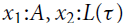 $x_1{:}A,x_2{:}L({\tau})$
. In the rule M:MatL, the initial potential defined by the annotation Q of the context
$x_1{:}A,x_2{:}L({\tau})$
. In the rule M:MatL, the initial potential defined by the annotation Q of the context
 $\Gamma,x{:}L({\tau})$
has to be sufficient to pay the costs of the evaluation of
$\Gamma,x{:}L({\tau})$
has to be sufficient to pay the costs of the evaluation of
 $e_1$
or
$e_1$
or
 $e_2$
(depending on whether the matched list is empty or not) and the potential defined by the annotation Q′ of the result type. To type the expression
$e_2$
(depending on whether the matched list is empty or not) and the potential defined by the annotation Q′ of the result type. To type the expression
 $e_1$
of the nil case, we use the projection
$e_1$
of the nil case, we use the projection
 $\pi^\Gamma_0 (Q)$
that results in an annotation for the context
$\pi^\Gamma_0 (Q)$
that results in an annotation for the context
 $\Gamma$
. To type the expression
$\Gamma$
. To type the expression
 $e_2$
of the cons case, we rely on the shift operation
$e_2$
of the cons case, we rely on the shift operation
 $\lhd_L(Q)$
for lists that results in an annotation for the context
$\lhd_L(Q)$
for lists that results in an annotation for the context
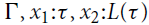 $\Gamma,x_1{:}A,x_2{:}L({\tau})$
.
$\Gamma,x_1{:}A,x_2{:}L({\tau})$
.
Like in the linear and univariate systems, sharing of variables is permitted but slightly more complex as we have to encode a basis transformation for higher-degree polynomials.
Example: Append Revisited
Consider again the functions append and alltails from the example in Section 5.1. In the univariate polynomial system, we derived the following types, considering quadratic and linear annotations. For simplicity, we assume that the element type A is the unit type
 $\mathbf{1}$
here.
$\mathbf{1}$
here.
 \[{append}: {{{L^{(c_{Cons_\mathbf{1}},0)}({\mathbf{1}})} \times {L^{(0,0)}({\mathbf{1}})}}}\buildrel {0/0} \over \longrightarrow{L^{(0,0)}({\mathbf{1}})}\]
 \[{alltails}: {L^{(0,c_{Cons_\mathbf{1}})}({\mathbf{1}})}\buildrel {0/0} \over \longrightarrow{L^{(0,0)}({\mathbf{1}})}\]
To express the equivalent potential annotations in the multivariate system, we can derive the types
 \[{append}: ({{L({\mathbf{1}})} \times {L({\mathbf{1}})}},Q) \to (L({\mathbf{1}}),Q') \quad \text{and} \quad {alltails}: (L({\mathbf{1}}),P) \to (L({\mathbf{1}}),P')\]
where
-
all constant annotation are zero, that is,
 $q_{([],[])} = q'_{[]} = p_{[]} = p'_{[]} = 0$
,
$q_{([],[])} = q'_{[]} = p_{[]} = p'_{[]} = 0$
, -
the non-constant potential assigned to the result of both functions is zero, that is,
$q'_{[*]} = q'_{[*,*]} = p'_{[*]} = p'_{[*,*]} = 0$
, -
the argument potential of append is linear in the first argument and zero otherwise, that is,
$q_{([*],[])} = c_{Cons_\mathbf{1}}$
and
$q_{([],[*])} = q_{([*,*],[])} = q_{([],[*,*])} = q_{([*],[*])} = 0$
, and -
the argument potential of alltails is quadratic, that is,
$p_{[*]} = 0$
and
$p_{[*,*]} = c_{Cons_\mathbf{1}}$
.
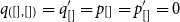
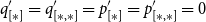


Now consider the case that we mentioned at the beginning of this subsection and consider the following function:
We can assign the type
 \[{f}: ({{L({\mathbf{1}})} \times {L({\mathbf{1}})}},Q) \to (L({\mathbf{1}}),Q')\]
where
 $q_{([*],[])} = c_{Cons_\mathbf{1}}$
,
$q_{([*],[])} = c_{Cons_\mathbf{1}}$
,
 $q_{([],[*])} = 0$
,
$q_{([],[*])} = 0$
,
 $q_{([*,*],[])} = q_{([],[*,*])} = q_{([*],[*])} = c_{Cons_\mathbf{1}}$
, and
$q_{([*,*],[])} = q_{([],[*,*])} = q_{([*],[*])} = c_{Cons_\mathbf{1}}$
, and
 $p_i = 0$
for all indices i. This is a tight bound that exactly reflects the cost
$p_i = 0$
for all indices i. This is a tight bound that exactly reflects the cost
 $(n + \binom{n+m}{2}) \cdot c_{Cons_\mathbf{1}}$
if n is the length of the first argument and m is the length of the second argument. Note that the cost
$(n + \binom{n+m}{2}) \cdot c_{Cons_\mathbf{1}}$
if n is the length of the first argument and m is the length of the second argument. Note that the cost
 $n \cdot c_{Cons_\mathbf{1}}$
is the cost of the call to append and
$n \cdot c_{Cons_\mathbf{1}}$
is the cost of the call to append and
 $\binom{n+m}{2} \cdot c_{Cons_\mathbf{1}}$
is the cost of the call to alltails.
$\binom{n+m}{2} \cdot c_{Cons_\mathbf{1}}$
is the cost of the call to alltails.
With the multivariate system, we are also able to derive most general type of append with quadratic annotations. We have
 \[{append}: ({{L({\mathbf{1}})} \times {L({\mathbf{1}})}},Q) \to (L({\mathbf{1}}),Q')\]
with the following constraints:
 \[\begin{array}{l@{}l@{}l} q_{([],[])} \geq q'_{[]}& q_{([*],[])} \geq q'_{[*]} + c_{Cons_\mathbf{1}}& q_{([],[*])} \geq q'_{[*]} \\ q_{([*,*],[])} \geq q'_{[*,*]}& q_{([*],[*])} \geq q'_{[*,*]}& q_{([],[*,*])} \geq q'_{[*,*]}\end{array}\]
Soundness
We can prove the familiar soundness theorem for AARA. The proof follows the same structure as for linear AARA.
[(Soundness of AARA)] Let
 $\Gamma;\, Q \vdash e : A$
and
$\Gamma;\, Q \vdash e : A$
and
 $V : \Gamma$
. If
$V : \Gamma$
. If
 $V \vdash e {\Downarrow {v}} \mid (p,\, p')$
for some v and
$V \vdash e {\Downarrow {v}} \mid (p,\, p')$
for some v and
 $(p,\, p')$
then
$(p,\, p')$
then
 $\Phi_V(\Gamma;\,Q) \geq p$
and
$\Phi_V(\Gamma;\,Q) \geq p$
and
 $\Phi_V(\Gamma;\,Q) - \Phi(v:A) \geq p - p'$
.
$\Phi_V(\Gamma;\,Q) - \Phi(v:A) \geq p - p'$
.
5.3 Beyond polynomial potential
AARA can also be used with non-polynomial potential functions. A key property for retaining compositionality is to identify function spaces for potential functions that are closed under operations like addition, multiplication, and composition. Another desired property is that potential functions decompose well when constructing and destructing data structures. For example, if f is a potential function and
 $a::as$
a non-empty list, then we would like to be able to express
$a::as$
a non-empty list, then we would like to be able to express
 $f(a::as) = \sum_{i} c_i g_i(a) + d_i h_i(as)$
as a weighted sum of potential functions
$f(a::as) = \sum_{i} c_i g_i(a) + d_i h_i(as)$
as a weighted sum of potential functions
 $g_i$
and
$g_i$
and
 $h_i$
for the head a and the tail as, respectively. Another consideration is the interaction with (multivariate) polynomial potential functions. Ideally, for a set of potential functions
$h_i$
for the head a and the tail as, respectively. Another consideration is the interaction with (multivariate) polynomial potential functions. Ideally, for a set of potential functions
 $\mathcal{P}$
there exists a function space with the aforementioned properties that includes both
$\mathcal{P}$
there exists a function space with the aforementioned properties that includes both
 $\mathcal{P}$
and the polynomial potential functions.
$\mathcal{P}$
and the polynomial potential functions.
Exponential Potential Functions
For exponential potential functions, Stirling numbers of the second kind have these desired properties. Stirling numbers of the second kind
 $\genfrac\{\}{0pt}{} n k = \frac 1 {k!} \sum_{i=0}^k ({-}1)^i \binom k i (k-i)^n$
count the number of ways to partition a set of n elements into k subsets. Recent work (Kahn and Hoffmann Reference Kahn and Hoffmann2020) uses Stirling numbers
$\genfrac\{\}{0pt}{} n k = \frac 1 {k!} \sum_{i=0}^k ({-}1)^i \binom k i (k-i)^n$
count the number of ways to partition a set of n elements into k subsets. Recent work (Kahn and Hoffmann Reference Kahn and Hoffmann2020) uses Stirling numbers
 $\genfrac\{\}{0pt}{} {n+1} {k+1}$
with arguments n,k offset by 1 as base functions. Potential functions for lists then have the form
$\genfrac\{\}{0pt}{} {n+1} {k+1}$
with arguments n,k offset by 1 as base functions. Potential functions for lists then have the form
 $\sum_i p_i \cdot \genfrac\{\}{0pt}{} {n+1}{i+1}$
, where n is the length of the list and
$\sum_i p_i \cdot \genfrac\{\}{0pt}{} {n+1}{i+1}$
, where n is the length of the list and
 $p_i \in {\mathbb{Q}_{\geq 0}}$
. In the type system, the coefficients
$p_i \in {\mathbb{Q}_{\geq 0}}$
. In the type system, the coefficients
 $p_i$
can be associated with list types
$p_i$
can be associated with list types
 $L^{\vec p}({A})$
like in the (univariate) polynomial case.
$L^{\vec p}({A})$
like in the (univariate) polynomial case.
Stirling numbers of the second kind satisfy the recurrence
 $\genfrac\{\}{0pt}{} {n+1} {k+1} = (k+1)\genfrac\{\}{0pt}{} n {k+1} + \genfrac\{\}{0pt}{} n k$
. This gives rise to a definition of a shift function that can be used to distribute potential when constructing or destructing lists. If a list
$\genfrac\{\}{0pt}{} {n+1} {k+1} = (k+1)\genfrac\{\}{0pt}{} n {k+1} + \genfrac\{\}{0pt}{} n k$
. This gives rise to a definition of a shift function that can be used to distribute potential when constructing or destructing lists. If a list
 $\ell:L^{\vec p}({A})$
is deconstructed in a pattern matching, then the tail of
$\ell:L^{\vec p}({A})$
is deconstructed in a pattern matching, then the tail of
 $\ell$
can be assigned the type
$\ell$
can be assigned the type
 $L^{\vec q}({A})$
such that
$L^{\vec q}({A})$
such that
 $q_i = (i+1)p_i + p_{i+1}$
. Here
$q_i = (i+1)p_i + p_{i+1}$
. Here
 $p_i$
and
$p_i$
and
 $q_i$
are the coefficients of
$q_i$
are the coefficients of
 $\genfrac\{\}{0pt}{} {n+1}{k+1}$
. This shift operation yields a linear relation, as the coefficient of a given
$\genfrac\{\}{0pt}{} {n+1}{k+1}$
. This shift operation yields a linear relation, as the coefficient of a given
 $p_i$
is a constant scalar. Thus, inference can again be automated via LP. Other exponential bases, like Gaussian binomial coefficients, could be similarly automated.
$p_i$
is a constant scalar. Thus, inference can again be automated via LP. Other exponential bases, like Gaussian binomial coefficients, could be similarly automated.
Because
 $\genfrac\{\}{0pt}{} {n+1}{k+1} = \frac 1 {k!} \sum_{i=0}^k (-1)^{k-i}\binom k i(i+1)^n \in \Theta((k+1)^n)$
, the offset Stirling numbers of the second kind can form a linear basis for the space of sums of exponential functions. Each function
$\genfrac\{\}{0pt}{} {n+1}{k+1} = \frac 1 {k!} \sum_{i=0}^k (-1)^{k-i}\binom k i(i+1)^n \in \Theta((k+1)^n)$
, the offset Stirling numbers of the second kind can form a linear basis for the space of sums of exponential functions. Each function
 $\lambda n.b^n$
with
$\lambda n.b^n$
with
 $b\geq 1$
can be expressed as a linear combination of the functions
$b\geq 1$
can be expressed as a linear combination of the functions
 $\lambda n.\genfrac\{\}{0pt}{} {n+1}{k+1}$
. The function
$\lambda n.\genfrac\{\}{0pt}{} {n+1}{k+1}$
. The function
 $\lambda n.\genfrac\{\}{0pt}{} {n+1}{k+1}$
is also non-negative for natural n and non-decreasing with respect to n. While there are exponential functions that cannot be expressed by the Stirling numbers, they form a maximally expressive basis in the following sense. It is not possible to express additional potential functions using a different basis without losing expressibility elsewhere. The standard exponential basis is not maximal in this sense (Kahn and Hoffmann Reference Kahn and Hoffmann2020).
$\lambda n.\genfrac\{\}{0pt}{} {n+1}{k+1}$
is also non-negative for natural n and non-decreasing with respect to n. While there are exponential functions that cannot be expressed by the Stirling numbers, they form a maximally expressive basis in the following sense. It is not possible to express additional potential functions using a different basis without losing expressibility elsewhere. The standard exponential basis is not maximal in this sense (Kahn and Hoffmann Reference Kahn and Hoffmann2020).
It is possible to combine the existing polynomial potential functions with these new exponential potential functions to not only conservatively extend both, but further represent potentials functions with their products. This leads to potential functions of the form
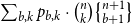 $\sum_{b,k} p_{b,k} \cdot \binom n k \genfrac\{\}{0pt}{} {n+1}{b+1}$
. It is straightforward to find a linear constraints that describe a shift operation for this basis.
$\sum_{b,k} p_{b,k} \cdot \binom n k \genfrac\{\}{0pt}{} {n+1}{b+1}$
. It is straightforward to find a linear constraints that describe a shift operation for this basis.
Logarithmic Potential Functions
While exponential potential might be required to type programs with overall polynomial resource consumption, it is arguable that logarithmic bounds and logarithmic potential functions are more relevant for many programs. Hofmann was in fact interested in logarithmic potential functions for many years and actively worked on this subject with Georg Moser prior to his death (Hofmann and Moser Reference Hofmann and Moser2018).
Logarithmic potential is particularly challenging in the context of AARA because it seems to usually require global reasoning (“split the list in the middle until it is empty”). This is in contrast to the polynomial and exponential case, where potential functions can be decomposed to a sum of potential for every sublist. More concretely, if we assign the potential
 $\log_2 n$
to a list, then difference
$\log_2 n$
to a list, then difference
 $\log_2 n - \log_2 (n-1)$
remains as a spill if we assign the same logarithmic potential to the tail of the list in a pattern match. This spill cannot be directly assigned to the tail of the list like in the polynomial case where, for example, the spill
$\log_2 n - \log_2 (n-1)$
remains as a spill if we assign the same logarithmic potential to the tail of the list in a pattern match. This spill cannot be directly assigned to the tail of the list like in the polynomial case where, for example, the spill
 $\binom{n}{2} - \binom{n-1}{2} = n-1$
can be directly assigned to the tail of a list.
$\binom{n}{2} - \binom{n-1}{2} = n-1$
can be directly assigned to the tail of a list.
To address this issue, Hofmann and Moser propose (Hofmann and Moser Reference Hofmann and Moser2018) to use potential functions
 \[p_{(a,b)} (\ell) =\log( a \cdot |\ell| + b )\]
for
 $a,b \geq 0$
.Footnote 6 When constructing or deconstructing a list, we can relate the potential of a list
$a,b \geq 0$
.Footnote 6 When constructing or deconstructing a list, we can relate the potential of a list
 $x::xs$
and its tail xs with the identity
$x::xs$
and its tail xs with the identity
 $p_{(a,b)} (x::xs) = p_{(a,b+a)}(xs)$
. The downsides of this approach are that inferring potential functions requires non-linear constraints and that it is not directly clear how to restrict the type system to a finite set of base functions.
$p_{(a,b)} (x::xs) = p_{(a,b+a)}(xs)$
. The downsides of this approach are that inferring potential functions requires non-linear constraints and that it is not directly clear how to restrict the type system to a finite set of base functions.
6. Lazy Evaluation and Co-Recursion
Lazy evaluation allows to defer the evaluation of subexpressions until the first time they are needed at runtime; these unevaluated subexpressions are referred to as thunks. Upon the first time a reference to a thunk is accessed, the subexpression in memory is replaced by the computed value, which is then readily available for subsequent accesses. Lazy evaluation enables the practical implementation of co-recursive algorithms that construct and work on possibly infinite data structures.
At first glance, a thunk can be treated like a function without an argument, similar to a function of type
 ${\mathbf{1}}\buildrel {q/0} \over \longrightarrow{A}$
. Accounting for lazy evaluation thus also requires the solutions needed to deal with higher-order AARA as well. A crucial point of lazy evaluation is that thunks that are not needed do not incur any evaluation cost. The AARA for lazy evaluation accounts for this in two ways:
${\mathbf{1}}\buildrel {q/0} \over \longrightarrow{A}$
. Accounting for lazy evaluation thus also requires the solutions needed to deal with higher-order AARA as well. A crucial point of lazy evaluation is that thunks that are not needed do not incur any evaluation cost. The AARA for lazy evaluation accounts for this in two ways:
-
(1) A constant part of a thunks evaluation cost may be paid through its q annotation, just like for a function of type
${\mathbf{1}}\buildrel {q/0} \over \longrightarrow{A}$
. However, treating a thunk like a function would imply that this cost is paid for every access to it. Instead, the q annotation may be prepaid at any time, effectively changing the thunks type to a function type similar to
${\mathbf{1}}\buildrel {0/0} \over \longrightarrow{A}$
, which can then be shared. The choice is either to pay the fixed cost q for every access or just once, the latter having the disadvantage that the cost is accounted for even if the thunk is never accessed at all. This decision can be left to the LP solver, which picks the solution that yields the overall lower cost bound. -
(2) Another part of a thunks evaluation cost may be paid through the potential captured in its closure. Since we know that a thunk is evaluated at most once, the types in its closure can safely be allowed to have potential, unlike for function closures requiring
as mentioned before. Even if a thunk references itself, there is no unsound duplication of potential: any thunk that needs to access itself before it is evaluated to weak-head normal form will never evaluate at all. Correspondingly, implementations of lazy evaluation usually mark all thunks currently under evaluation to prevent entering indefinite loops, a technique commonly referred to as black-holing. The invariant used in the soundness proof of the AARA for lazy evaluation similarly uses black-holing to track the potential within self-referencing thunk closures.


First explored by Hugo Simões, it turned out to be quite difficult to find a suitable invariant for the soundness proof of the AARA for a lazily evaluated language (Simões et al. Reference Simões, Vasconcelos, Florido, Jost and Hammond2012; Simões Reference Simões2014).
Building on this, the successful analysis of co-recursive programs required an even more intricate proof invariant. The key idea was to track a single type A per memory location, whose potential must then share to the multi-set of types
 $A_1,\dots,A_i$
associated with all mutually existing references to that location, that is,
$A_1,\dots,A_i$
associated with all mutually existing references to that location, that is,
![]() must be satisfied (Jost et al. Reference Jost, Vasconcelos, Florido and Hammond2017; Vasconcelos et al. Reference Vasconcelos, Jost, Florido and Hammond2015). In retrospective, it turned out that this condition is somewhat similar to the write-view in the object-oriented setting.
must be satisfied (Jost et al. Reference Jost, Vasconcelos, Florido and Hammond2017; Vasconcelos et al. Reference Vasconcelos, Jost, Florido and Hammond2015). In retrospective, it turned out that this condition is somewhat similar to the write-view in the object-oriented setting.
The resulting AARA is then capable to infer, for an example, that function repeat has finite heap-space usage, while repeat’ has an infinite hunger for heap space. Note that both functionsFootnote 7 are functionally indistinguishable:
7. Imperative Programs
AARA is mostly associated with type systems for functional languages, following the original presentation of Hofmann and Jost (Reference Hofmann and Jost2003). However, the technique can also be integrated with program logics for programs that modify state. If potential is associated with data structures, then separation logic is a natural framework for introducing potential, as explored by Atkey (Reference Atkey2010). If potential is associated with integers, then a standard Hoare logic can be the foundation for an automatic analysis (Carbonneaux et al. Reference Carbonneaux, Hoffmann and Shao2015; Carbonneaux et al. Reference Carbonneaux, Hoffmann, Reps and Shao2017). Moreover, Hofmann and his collaborators have applied AARA to object-oriented languages (Bauer and Hofmann Reference Bauer, Hofmann, Eiter and Sands2017; Bauer et al. Reference Bauer, Jost, Hofmann, Sutcliffe and Veanes2018; Bauer Reference Bauer2019; Hofmann and Jost Reference Hofmann and Jost2006; Hofmann and Rodriguez Reference Hofmann and Rodriguez2009; Rodriguez Reference Rodriguez2012).
Separation Logic
Separation logic is a program logic for succinctly reasoning about mutable data structures and pointers (Ishtiaq and O’Hearn Reference Ishtiaq and O’Hearn2001; Reynolds Reference Reynolds2002). A key concept is the separating conjunction
 $P * Q$
, which is satisfied by a program state if it can be split into two disjoint parts such that one part satisfies P and the other part satisfies Q. For example, a linked list can be specified by the (recursive) formula
$P * Q$
, which is satisfied by a program state if it can be split into two disjoint parts such that one part satisfies P and the other part satisfies Q. For example, a linked list can be specified by the (recursive) formula
 \[\text{lseg}(x,y) \triangleq ( x=y \land \text{emp}) \lor (\exists \, d,z \, . \, x \mapsto (d,z) * \text{lseg}(z,y)) \; .\]
Here, x, y, and z are memory addresses on the heap and
 $x \mapsto (d,z)$
expresses that address x contains the pair (d,z). To satisfy this formula, either
$x \mapsto (d,z)$
expresses that address x contains the pair (d,z). To satisfy this formula, either
 $x=y$
and the list is empty (emp is satisfied by an empty heap) or the heap can be split into two disjoint parts: the first part contains head at address x and the second contains the tail, starting at address z and ending at address y.
$x=y$
and the list is empty (emp is satisfied by an empty heap) or the heap can be split into two disjoint parts: the first part contains head at address x and the second contains the tail, starting at address z and ending at address y.
Atkey (Reference Atkey2010) extended machine states with non-negative numbers that represent the available potential and separation logic with a predicate
 $\diamond$
that can be satisfied by one potential unit in the machine state. When used in a separating conjunction
$\diamond$
that can be satisfied by one potential unit in the machine state. When used in a separating conjunction
 $P * \diamond$
, the state has to be split into one potential unit and an empty heap to satisfy
$P * \diamond$
, the state has to be split into one potential unit and an empty heap to satisfy
 $\diamond$
, and the remaining heap and potential units to satisfy P. For example, a list with two potential units per element can be specified with the following formula:
$\diamond$
, and the remaining heap and potential units to satisfy P. For example, a list with two potential units per element can be specified with the following formula:
 \[\text{lseg}_2(x,y) \triangleq ( x=y \land \text{emp}) \lor (\exists \, d,z \, . \, x \mapsto (d,z) * \diamond * \diamond * \text{lseg}_2(z,y)) \; .\]
While the heap is treated linearly in separation logic, potential can be treated as an affine resource. The potential annotations can also be inferred via LP like in the linear case (Atkey Reference Atkey2010).
Such diamond predicates have been used with concurrent separation logic to verify progress properties of non-blocking concurrent data structures (Hoffmann et al. Reference Hoffmann, Marmar and Shao2013). An extended version of this separation logic has been implemented in the Coq proof assistant to prove tight bounds on complex data structure operations such as union-find (Charguéraud and Pottier Reference Charguéraud and Pottier2019; Mével et al. Reference Mével, Jourdan and Pottier2019).
Quantitative Hoare Logic and Integers
Similarly, potential functions can also be integrated in Hoare logic. Carbonneaux et al. (Reference Carbonneaux, Hoffmann, Ramananandro and Shao2014); Carbonneaux et al. (Reference Carbonneaux, Hoffmann and Shao2015) have introduced a Hoare logic where predicates map states to non-negative numbers instead of Booleans as in standard Hoare logic. Using these predicates, a quantitative Hoare triple
 ${{\{{\Phi}\}\, {S}\, \{{\Phi'}\}}} $
is valid if
${{\{{\Phi}\}\, {S}\, \{{\Phi'}\}}} $
is valid if
 $\Phi(\sigma) \ge n + \Phi'(\sigma')$
for all states
$\Phi(\sigma) \ge n + \Phi'(\sigma')$
for all states
 $\sigma$
and
$\sigma$
and
 $\sigma'$
such that
$\sigma'$
such that
 $(S, \sigma) \Downarrow_n \sigma'$
. Here,
$(S, \sigma) \Downarrow_n \sigma'$
. Here,
 $(S, \sigma) \Downarrow_n \sigma'$
is an evaluation judgment that expresses that the statement S evaluates to state
$(S, \sigma) \Downarrow_n \sigma'$
is an evaluation judgment that expresses that the statement S evaluates to state
 $\sigma'$
using n resources if executed in state
$\sigma'$
using n resources if executed in state
 $\sigma$
. Like in the functional case,
$\sigma$
. Like in the functional case,
 $\Phi(\sigma)$
must provide sufficient potential for covering the resource cost of the execution and the potential
$\Phi(\sigma)$
must provide sufficient potential for covering the resource cost of the execution and the potential
 $\Phi'(\sigma')$
.
$\Phi'(\sigma')$
.
Quantitative Hoare triples enable us to reason compositionally about sequential compositions
 $S_1;\,S_2$
. If
$S_1;\,S_2$
. If
 $(\sigma, S_1) \Downarrow_n \sigma'$
and
$(\sigma, S_1) \Downarrow_n \sigma'$
and
 $(\sigma', S_2) \Downarrow_m \sigma''$
, we get
$(\sigma', S_2) \Downarrow_m \sigma''$
, we get
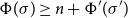 $\Phi(\sigma) \ge n + \Phi'(\sigma')$
,
$\Phi(\sigma) \ge n + \Phi'(\sigma')$
,
 $\Phi'(\sigma') \ge m + \Phi''(\sigma'')$
, and thus
$\Phi'(\sigma') \ge m + \Phi''(\sigma'')$
, and thus
 $\Phi(\sigma) \ge (n + m) + \Phi''(\sigma'')$
. This provides the justification for the following familiar looking rule:
$\Phi(\sigma) \ge (n + m) + \Phi''(\sigma'')$
. This provides the justification for the following familiar looking rule:
 $${{\{ \Phi \} {\mkern 1mu} {S_1}{\mkern 1mu} \{ \Phi '\} \quad \{ \Phi '\} {\mkern 1mu} {S_2}{\mkern 1mu} \{ \Phi ''\} } \over {\{ \Phi \} {\mkern 1mu} {S_1};{S_2}{\mkern 1mu} \{ \Phi ''\} }}$$
. In the previous rule,
 $\Phi$
gives a bound for
$\Phi$
gives a bound for
 $S_1;\, S_2$
through the intermediate potential
$S_1;\, S_2$
through the intermediate potential
 $\Phi'$
, even though it was derived on
$\Phi'$
, even though it was derived on
 $S_1$
only. For loops, the potential functions before and after the loop body have to be identical, similar to an invariant.
$S_1$
only. For loops, the potential functions before and after the loop body have to be identical, similar to an invariant.
The derivation of a resource bound using potential functions is best explained by example. If we use the tick metric that assigns cost n to the function call tick(n) and cost 0 to all other operations, then the resource consumption of the following statement is
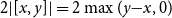 $2|[x,y]| = 2\max(y{-}x,0)$
:
$2|[x,y]| = 2\max(y{-}x,0)$
:
Figure 3 shows a derivation of this bound in the quantitative Hoare logic. We start with the initial potential
 $\Phi_0 = 2|[x,y]|$
, which we also use as the loop invariant. For the loop body, we must derive a triple
$\Phi_0 = 2|[x,y]|$
, which we also use as the loop invariant. For the loop body, we must derive a triple
 ${{\{{\Phi_0}\}\, {{x=x+1;tick(1)}}\, \{{\Phi_0}\}}}$
. We start with the potential
${{\{{\Phi_0}\}\, {{x=x+1;tick(1)}}\, \{{\Phi_0}\}}}$
. We start with the potential
 $2|[x,y]|$
and the fact that
$2|[x,y]|$
and the fact that
 $|[x,y]| > 0$
before the assignment. If we denote the updated version of x after the assignment by x′, then the relation
$|[x,y]| > 0$
before the assignment. If we denote the updated version of x after the assignment by x′, then the relation
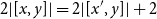 $2|[x,y]| = 2|[x',y]| + 2$
between the potential before and after the assignment x=x+1 holds. This means that we have the potential
$2|[x,y]| = 2|[x',y]| + 2$
between the potential before and after the assignment x=x+1 holds. This means that we have the potential
 $2|[x,y]| + 2$
before the statement tick(2). Since tick(2) consumes 2 resource units, we end up with potential
$2|[x,y]| + 2$
before the statement tick(2). Since tick(2) consumes 2 resource units, we end up with potential
 $2|[x,y]|$
after the loop body and have established the loop invariant again.
$2|[x,y]|$
after the loop body and have established the loop invariant again.
Derivation of a tight bound on the number of ticks for a for loop. The parameters
 $K>0$
and
$K>0$
and
 $T>0$
denote concrete but arbitrary constants.
$T>0$
denote concrete but arbitrary constants.

To automatically find derivations in the quantitative logic, we can start with template propositions that contain unknown coefficients for each potential assertion. One possibility is to use potential functions that are non-negative linear combinations
 $q_1 |[x,y]| + q_2 |[y,x] + q_3 |[z,y]|$
of interval sizes (Carbonneaux et al. Reference Carbonneaux, Hoffmann and Shao2015). Another, more flexible approach is to use general polynomials in integer variables (Carbonneaux et al. Reference Carbonneaux, Hoffmann, Reps and Shao2017). General polynomials create the obligation to ensure that potential is non-negative. While it is possible to allow negative potential when deriving a bound on the net cost (as opposed to the high watermark, i.e. the maximum amount of simultaneously used resources, thus including all temporarily used resources that are released again before the end of execution), one still has to ensure the soundness of the weakening rule by preventing the “waste” of negative potential.
$q_1 |[x,y]| + q_2 |[y,x] + q_3 |[z,y]|$
of interval sizes (Carbonneaux et al. Reference Carbonneaux, Hoffmann and Shao2015). Another, more flexible approach is to use general polynomials in integer variables (Carbonneaux et al. Reference Carbonneaux, Hoffmann, Reps and Shao2017). General polynomials create the obligation to ensure that potential is non-negative. While it is possible to allow negative potential when deriving a bound on the net cost (as opposed to the high watermark, i.e. the maximum amount of simultaneously used resources, thus including all temporarily used resources that are released again before the end of execution), one still has to ensure the soundness of the weakening rule by preventing the “waste” of negative potential.
7.1 Object-oriented programs
Several research works are dedicated to adapt AARA to an object-oriented imperative setting: Hofmann and Jost (Reference Hofmann and Jost2006), Hofmann and Rodriguez (Reference Hofmann and Rodriguez2009), Rodriguez (Reference Rodriguez2012), Bauer and Hofmann (Reference Bauer, Hofmann, Eiter and Sands2017), Bauer et al. (Reference Bauer, Jost, Hofmann, Sutcliffe and Veanes2018), Bauer (Reference Bauer2019). A major difference in this setting being that circular references are highly common place, whereas these only occur in the functional setting concerned with co-recursion and lazy evaluation.
Consider, for example, a doubly linked list with at least three elements: any element can then be referenced through an infinite number of access paths of arbitrary length, each going back-and-forth between the same three nodes. This is a problem for AARA, since potential is crucially counted by reference-path, as pointed out earlier in Section 3.5. An infinite amount of references to a single memory location then implies that only a finite amount of these reference-paths may be awarded potential, since an otherwise infinite potential would lead to a useless infinite upper bound.
The key idea from Hofmann and Jost (Reference Hofmann and Jost2006) is to track two types for each entity, one for writing and one for reading. The writing type must share to all existing reading types, thereby ensuring that potential is soundly conserved. The different types for an object are referred to as “Views” on that entity, which form a hierarchy of diminishing potential. In the case of circular structures, each reference will lead to a structure of overall decreased potential, until the last view holds no more potential and thus freely shares to an infinite amount of references as needed.
The inference must determine not only the annotated types but also the number of required views and thus becomes much more difficult: it requires solving pointwise linear inequalities between infinite trees labeled with non-negative rational numbers. In general, this is at least as hard as solving the Skolem–Mahler–Lech problem, as shown by Bauer (Reference Bauer2019). However, Bauer could also surprisingly show that the constraints generated by the AARA are once more of a benign shape, such that satisfiability is indeed decidable (Bauer et al. Reference Bauer, Jost, Hofmann, Sutcliffe and Veanes2018), neatly mirroring the observation from the first paper (Hofmann and Jost Reference Hofmann and Jost2003), where the generated ILP turned out to be only as difficult as the LP.
8. Parallel Evaluation and Concurrency
Apart from strict and lazy evaluation, AARA is also applicable to parallel evaluation (Hoffmann and Shao Reference Hoffmann and Shao2015) and concurrent programs using session types (Das et al. Reference Das, Hoffmann and Pfenning2018).
Parallel Evaluation
In parallel evaluation, we allow two subexpressions of an expression that do not depend on each others result to be evaluated in parallel. The exact cost of parallel evaluation depends on the underlying hardware features like the number of processor cores. However, we can avoid reasoning about these low-level details by deriving bounds on a more abstract cost model that consists of the work and the depth of an evaluation of a program (Blelloch and Greiner Reference Blelloch and Greiner1996). Work measures the evaluation time of sequential evaluation and depth measures the evaluation time of parallel evaluation assuming an unlimited number of processors. One can show (see, e.g., Harper Reference Harper2012) that a program that evaluates to a value using work w and depth d can be evaluated on a shared-memory multiprocessor system with p processors in time
 $K\cdot\max(\frac{w}{p},d)$
for some fixed constant K.
$K\cdot\max(\frac{w}{p},d)$
for some fixed constant K.
To derive a bound on the work, we can simply apply (sequential) AARA. To derive a bound on a parallel composition, we need to compose potential functions using
 $\max$
instead of addition like in sequential composition. However, a complication arises since potential is not only used to cover the evaluation cost but also to assign potential to resulting data structures. A naive use of the maximum would therefore be unsound.
$\max$
instead of addition like in sequential composition. However, a complication arises since potential is not only used to cover the evaluation cost but also to assign potential to resulting data structures. A naive use of the maximum would therefore be unsound.
One solution (Hoffmann and Shao Reference Hoffmann and Shao2015) is to use cost-free typings to reason about parallel composition. A cost-free typing is a type derivation in AARA with respect to the cost-free resource metric that assigns cost 0 to every operation. While cost-free typings can trivially assign 0 to every potential annotations, they can express how to soundly transfer potential from the inputs of the inputs of a computation to its result.
Hoffmann and Shao (Reference Hoffmann and Shao2015) applied this idea to a language with binary fork-join parallelism. Parallel computation is explicitly introduced with a parallel let binding of the form
 \[\mathop{\,\mathsf{par}\,} x_1 = e_1 \mathop{\,\mathsf{and}\,} x_2 = e_2 \mathop{\,\mathsf{in}\,} e \;\]
In the typing rule, we would type
 $e_1$
and
$e_1$
and
 $e_2$
twice: First, we split the potential in the context to type
$e_2$
twice: First, we split the potential in the context to type
 $e_1$
with the regular cost metric and
$e_1$
with the regular cost metric and
 $e_2$
with the cost-free metric. Second, we split the potential in the context to type
$e_2$
with the cost-free metric. Second, we split the potential in the context to type
 $e_1$
with the cost-free metric and
$e_1$
with the cost-free metric and
 $e_2$
with the regular metric. This rule is compatible with the type rules for sequential computation, and the structure of the soundness proof remains unchanged.
$e_2$
with the regular metric. This rule is compatible with the type rules for sequential computation, and the structure of the soundness proof remains unchanged.
Session Types
To reason about the work cost of concurrent processes, the potential method of AARA can be integrated with session types (Honda Reference Honda and Best1993; Honda et al. Reference Honda, Vasconcelos, Kubo and Hankin1998). Session types specify communication protocols between message-passing processes, and the type rules ensure that well-typed processes follow these protocols.
AARA has been successfully integrated with binary session types that are based on intuitionistic linear logic (Pfenning and Griffith Reference Pfenning and Griffith2015) to reason about the work performed by concurrent systems (Das et al. Reference Das, Hoffmann and Pfenning2018). Session types and AARA fit together seamlessly since both are based on substructural logics. Apart from the traditional advantages of AARA, like type inference with LP and amortized reasoning, resource-aware session types are naturally compositional. The key is that processes can store potential and that potential can be transferred between processes. In this way, session-typed protocols can contain payment schemes where processes have to send potential to cover the cost that is incurred at the receiving process by sending a certain message.
Resource-aware session types find applications in programming digital contracts (Das et al. Reference Das, Balzer, Hoffmann, Pfenning and Santurkar2021) in which resource (or “gas”) consumption plays a prominent role in protecting against denial-of-service attacks.
9. Probabilistic Programming
AARA has also been applied to derive bounds on the (worst-case) expected cost of imperative (Ngo et al. Reference Ngo, Carbonneaux and Hoffmann2018) and functional (Wang et al. Reference Wang, Kahn and Hoffmann2020) probabilistic programs. Probabilistic programs are equipped with probabilistic branching and sampling expressions and describe distributions over possible results. For example, a functional language can be extended with a syntactic form
 \[\mathop{\,\mathsf{flip}\,} p \; \{H \hookrightarrow e_1 \mid T \hookrightarrow e_2\}\]
for probabilistic branching, where
 $p \in [0,1]$
is a probability and
$p \in [0,1]$
is a probability and
 $e_1,e_2$
are expressions. The semantics expression is that
$e_1,e_2$
are expressions. The semantics expression is that
 $e_1$
is evaluated with probability p and
$e_1$
is evaluated with probability p and
 $e_2$
is evaluated with probability
$e_2$
is evaluated with probability
 $1-p$
. For example, the function bernoulli below implements a Bernoulli process across the elements of an input list. It terminates with probability 1 and has worst-case cost
$1-p$
. For example, the function bernoulli below implements a Bernoulli process across the elements of an input list. It terminates with probability 1 and has worst-case cost
 $1 \cdot |{lst}|$
. However, the expected cost of bernoulli is only 1.
$1 \cdot |{lst}|$
. However, the expected cost of bernoulli is only 1.
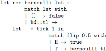
To derive the tight bound 1 on the expected cost, we use the following typing rule for flip expressions:

To understand the rule, consider the expression
 $\mathop{\,\mathsf{flip}\,} p \; \{H \hookrightarrow e_1 \mid T \hookrightarrow e_2\}$
and assume that
$\mathop{\,\mathsf{flip}\,} p \; \{H \hookrightarrow e_1 \mid T \hookrightarrow e_2\}$
and assume that
 $e_1$
requires
$e_1$
requires
 $\Phi_1$
units of potential and
$\Phi_1$
units of potential and
 $e_2$
requires
$e_2$
requires
 $\Phi_2$
units of potential. The evaluation of the flip expression requires a weighted average of
$\Phi_2$
units of potential. The evaluation of the flip expression requires a weighted average of
 $\Phi_1$
and
$\Phi_1$
and
 $\Phi_2$
, specifically
$\Phi_2$
, specifically
 $p \cdot \Phi_1 + (1-p) \cdot \Phi_2$
. This should be covered by the typing context
$p \cdot \Phi_1 + (1-p) \cdot \Phi_2$
. This should be covered by the typing context
 $\Gamma$
and constant potential q, both of which are shared between branches. The distribution of this sharing is expressed using a sharing relation
$\Gamma$
and constant potential q, both of which are shared between branches. The distribution of this sharing is expressed using a sharing relation
![]() , which apportions the potential indicated by τ into two parts to be associated with
, which apportions the potential indicated by τ into two parts to be associated with
 $\tau_1$
and
$\tau_1$
and
 $\tau_2$
, alongside a potential-scaling operation.
$\tau_2$
, alongside a potential-scaling operation.
Proving the soundness of the expected resource analysis is more challenging than in the deterministic case. It relies on a probabilistic operational cost semantics based on Borgström et al.’s trace-based and step-indexed-distribution-based semantics (Borgström et al. Reference Borgström, Dal Lago, Gordon and Szymczak2016). It is also possible to assign potential to symbolic probabilities (Wang et al. Reference Wang, Kahn and Hoffmann2020). However, automatic inference is still possible using linear constraints only.
10. Sponsored Research Projects
AARA was used notably within the following research projects:
Project Mobile Resource Guarantees
The “Mobile Resource Guarantees” (MRG) project (Mobile Resource Guarantees 2002-2005) was funded from 2002 to 2005 under the EU FP5-IST funding scheme with a budget of 1.252.000 EUR. Principal investigators were Don Sanella (Coordinator), David Aspinall, Stephen Gilmore, Ian Stark from the University of Edinburgh, and Martin Hofmann from LMU Munich. A total of 19 researchers were involved.
MRG developed the infrastructure needed to endow mobile code with independently verifiable certificates describing its resource behavior (space, time, etc.). These certificates are condensed and formalized mathematical proofs of a resource-related property which are by their very nature self-evident and unforgeable (proof-carrying code). Arbitrarily complex methods may be used by the code producer to construct these certificates, but their verification by the code consumer will always be a simple computation.
One way to produce proofs of resource bounds was provided by the available AARA at the time, which was implemented as a part of the Camelot compiler produced within the project. The bytecode produced by the compiler included a protected encoding of the annotated type derivation. The proof lies then in the verification that the supplied annotated type derivation complies with the AARA type rules and fits the program, which is significantly easier as a full annotated type inference.
Project EmBounded
The “EmBounded” project (Embounded 2005-2008) was funded from 2005 to 2008 under the EU FP6-IST funding scheme with a budget of 1.479.377 EUR. Principal investigators were Kevin Hammond (Coordinator), Roy Dyckhoff from St Andrews; Greg Michaelson, Andrew Wallace from Heriot-Watt; Martin Hofmann, Hans-Wolfgang Loidl from LMU Munich; Jocelyn Sérot from Lasmea, Clermont-Ferrand; Christian Ferdinand, and Reinhold Heckmann from AbsInt GmbH, Saarbrücken. Several more researchers contributed to the project for a total of at least 190.5 person-months.
EmBounded identified, quantified, and certified resource bounds for a domain-specific high-level programming languages called “Hume” which is targeted at real-timed embedded system. The AARA at the time was implemented into the compiler produced within the project; numerous resource metrics were available: heap- and stack-space usage as well as WCET.
Within the EmBounded project, WCET is measured in actual processor clock cycles for the target processor Renesas M32C/85. All possible building blocks produced by the Hume compiler were analyzed on the low level by the experts at AbsInt GmbH, Saarbrücken, giving fixed WCET bounds for each block using abstract interpretation methods. This information was then lifted to the high-level language through the cost constants of the AARA depicted earlier. For this to be precise, some cost constants had to be parameterized further, for example, the number of clock cycles required for returning after calls, branching operations or even subexpressions (
 $c_{\text{Let3}}$
), depends on the total number of return labels within the entire program (Jost et al. Reference Jost, Loidl, Hammond, Scaife and Hofmann2009a; Jost et al. Reference Jost, Loidl, Scaife, Hammond, Michaelson and Hofmann2009b). The implementations thus required a great deal of attention to details. The combined analysis delivered a WCET bound less than 34% above the worst measured runtime for the programs considered in the project, such as an inverted pendulum controller and line tracking by image recognition.
$c_{\text{Let3}}$
), depends on the total number of return labels within the entire program (Jost et al. Reference Jost, Loidl, Hammond, Scaife and Hofmann2009a; Jost et al. Reference Jost, Loidl, Scaife, Hammond, Michaelson and Hofmann2009b). The implementations thus required a great deal of attention to details. The combined analysis delivered a WCET bound less than 34% above the worst measured runtime for the programs considered in the project, such as an inverted pendulum controller and line tracking by image recognition.
11. Conclusion
In the past two decades, AARA grew from Hofmann’s ideas for implicitly characterizing the complexity class PTIME into an active research area that studies the (automatic) analysis of the resource requirements of programs. AARA evolves steadily and preserves the principles that have been established in Hofmann and Jost’s seminal work (Hofmann and Jost Reference Hofmann and Jost2003): local inference rules and easily checkable bound derivations, a soundness proof with respect to a cost semantics, amortized reasoning, and bound inference via numeric optimization.
We and many others who work on AARA have been inspired not only by Hofmann’s works but also by his vision, ambition, and optimism. While there has been great progress in automatic resource analysis, many open problems remain. Among them are smoothly integrating manual and automatic analyses, automating bound inference for object-oriented programs, and taking into account automatic memory management. We hope that this survey will be of use for identifying and ultimately solving such open problems, and that Hofmann’s work will continue to inspire researchers in this area.
Acknowledgements
We thank the reviewers for their constructive and detailed feedback, which helped to improve this survey article. The first author has been supported by the National Science Foundation under CAREER Award 1845514 and SHF Award 2007784. Any opinions, findings, and conclusions contained in this document are those of the authors and do not necessarily reflect the views of the sponsoring organizations.
Conflicts of Interest
The authors declare none.

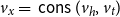


 Open access