


1. Introduction
Supersonic jet aircraft are typically propelled by turbofan engines having lower bypass ratios than modern subsonic aircraft. With reduced bypass ratio typically comes an increase in thrust-specific jet noise. This trend may lead future civilian supersonic jet aircraft to struggle to meet stringent noise regulations at take-off and landing. However, substantial improvements may be made by using internally mixed nozzles.
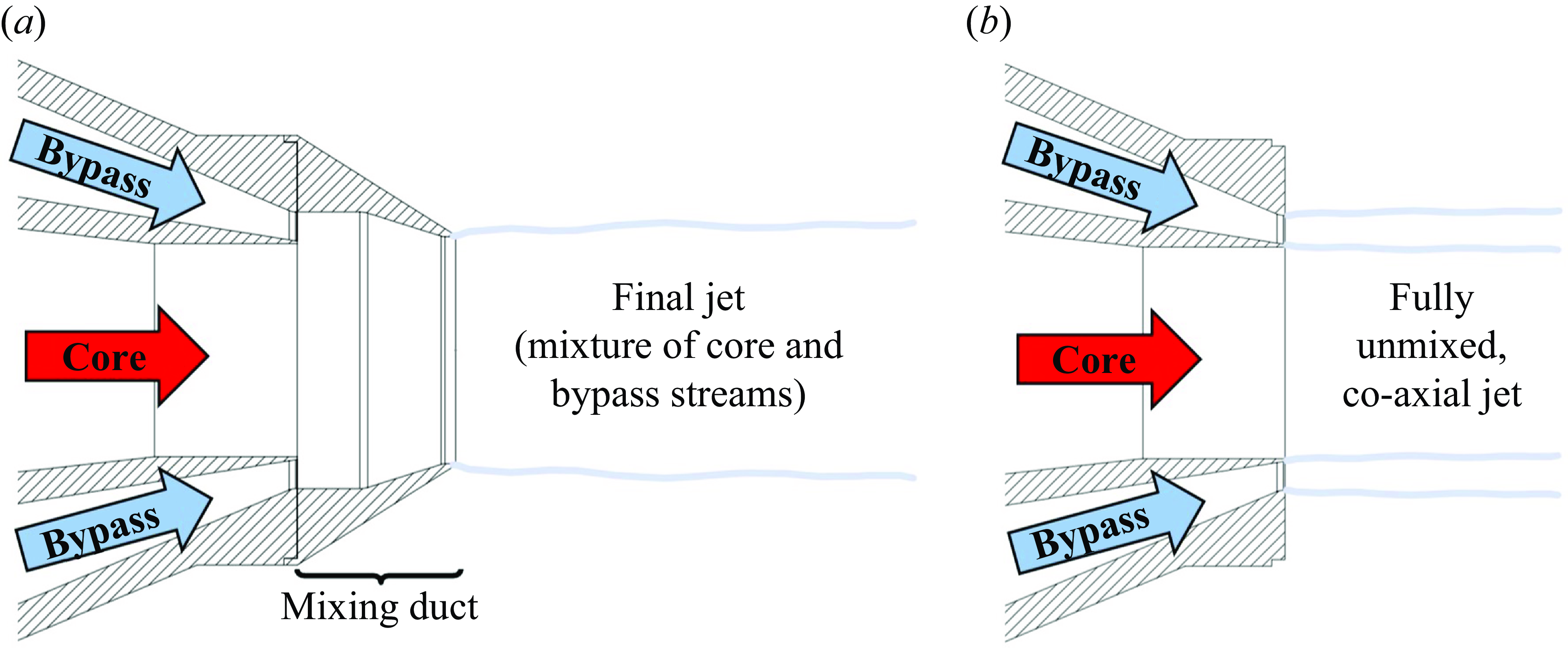
A dual-stream, internally mixed nozzle is illustrated by figure 1(a). An inner ‘core’ stream and an outer ‘bypass’ stream are routed into a mixing duct, where the two streams of gas mix to some degree before they are expanded from a final nozzle. The internal mixing can offer thrust-specific jet-noise reductions (e.g. see Pearson (Reference Pearson1962); Frost (Reference Frost1966); Shumpert (Reference Shumpert1980); Goodykoontz (Reference Goodykoontz1982); Mengle et al. (Reference Mengle, Dalton, Bridges and Boyd1997); Bridges & Wernet (Reference Bridges and Wernet2021)) by reducing the jet velocity of the heated core stream. In separate-flow nozzles, on the other hand, the core stream and bypass stream emerge from the nozzle entirely unmixed, as illustrated by figure 1(b). The separate-flow nozzle shown is simply the internally mixed nozzle from figure 1(a) with the mixing duct (which is a single component including the final nozzle’s contraction for the configuration shown) removed for illustrative purposes.
Dual-stream nozzle architectures: (a) internally mixed and (b) separate flow.
In prior model-scale experiments, Ramsey et al. (Reference Ramsey, Mayo, Karon, Funk and Ahuja2022b ) found that the jet from an axisymmetric, internally mixed nozzle (also referred to as a ‘confluent’ nozzle) howled loudly at certain jet operating conditions. The word ‘howling’ is used to convey that the generated noise was dominated by high-amplitude discrete tones. The term is general and is not meant to convey a specific type of resonance. ‘Screech’ would convey this equally well but is avoided due to that word’s use by the aeroacoustics community to refer to a resonance mechanism in the plume of imperfectly expanded supersonic jets (e.g. see early work by Powell (Reference Powell1953b ) and review articles by Raman (Reference Raman1999) and Edgington-Mitchell (Reference Edgington-Mitchell2019)). The jet operating conditions of interest to Ramsey et al. (Reference Ramsey, Mayo, Karon, Funk and Ahuja2022b ) were restricted to sonic and subsonic jet Mach numbers, focusing on jet noise at operating conditions relevant to take-off and landing.
The present paper deals with the exact same nozzle (described in greater detail in § 1.1) and howling as described by Ramsey et al. (Reference Ramsey, Mayo, Karon, Funk and Ahuja2022b ). Being axisymmetric, the nozzle studied was intended as a simple baseline for future research on internally mixed nozzles in which the trailing edge of the core nozzle is lobed rather than circular. Such geometries enhance the mixing of the two streams, and are more likely to be employed in the aircraft industry. Even in future research, however, axisymmetric configurations offer a valuable baseline against which the thrust and noise produced by more-sophisticated nozzles may be evaluated.
1.1. The model-scale nozzle
The nozzle used in the present study is shown in figure 2(a), and comprised two axisymmetric, coaxial flow paths which routed two streams of air into a round mixing duct with diameter $D_2 = 52.6$
mm. The area ratio between the upstream plenum chambers and the mixing-duct inlets were in excess of 30 : 1 for the core stream and 200 : 1 for the bypass stream. The core nozzle had exit diameter
$D_2 = 52.6$
mm. The area ratio between the upstream plenum chambers and the mixing-duct inlets were in excess of 30 : 1 for the core stream and 200 : 1 for the bypass stream. The core nozzle had exit diameter $D_1 = 40.6$
mm and lip thickness
$D_1 = 40.6$
mm and lip thickness $\delta _0 = 0.5$
mm. The ratio of the bypass-flow area to the core-flow area at the inlet to the mixing duct (accounting for the thickness of the core-nozzle lip) was 0.62. After the two streams met inside the mixing duct, the composite flow was expanded through a final, convergent-straight nozzle with a further 1.48 : 1 area contraction. The final nozzle’s converging angle was 17.4
$\delta _0 = 0.5$
mm. The ratio of the bypass-flow area to the core-flow area at the inlet to the mixing duct (accounting for the thickness of the core-nozzle lip) was 0.62. After the two streams met inside the mixing duct, the composite flow was expanded through a final, convergent-straight nozzle with a further 1.48 : 1 area contraction. The final nozzle’s converging angle was 17.4 $^{\circ }$
relative to the nozzle centreline, and the bend between the converging and final straight sections of the final nozzle had a radius of 2.54 mm.
$^{\circ }$
relative to the nozzle centreline, and the bend between the converging and final straight sections of the final nozzle had a radius of 2.54 mm.
Cross-sectional views of nozzle used: (a) nozzle assembly, (b) $L_e/D_e$
= 0.7 mixing-duct length with dimensions and coordinate conventions shown and (c)
$L_e/D_e$
= 0.7 mixing-duct length with dimensions and coordinate conventions shown and (c) $L_e/D_e$
= 3.0 mixing-duct length.
$L_e/D_e$
= 3.0 mixing-duct length.
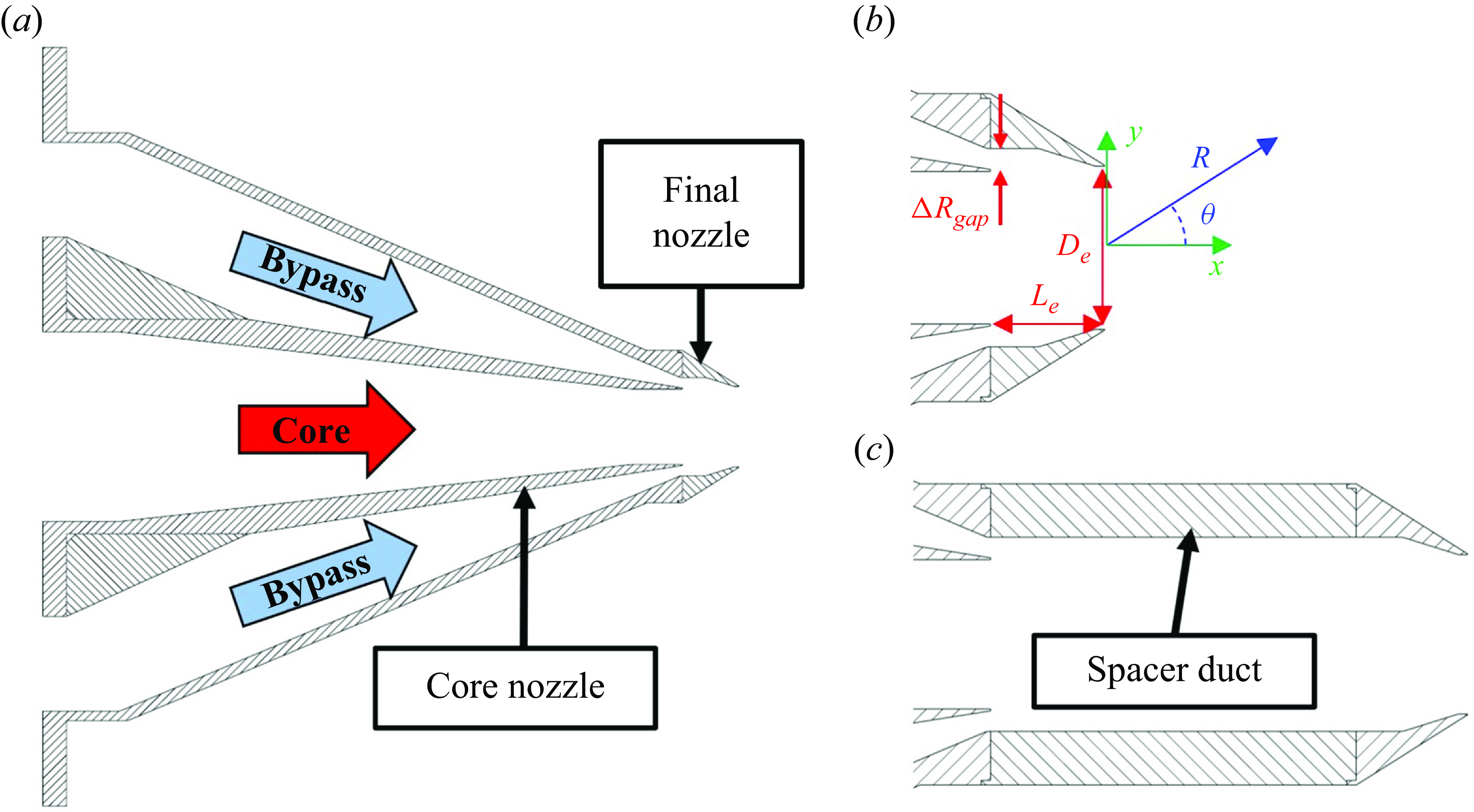
Figure 2(b) shows a close-up view of the far-downstream portion of the nozzle, along with important nozzle dimensions and coordinate conventions. The $x{-}y$
coordinates will appear in this paper along with flow measurements and
$x{-}y$
coordinates will appear in this paper along with flow measurements and $R-\theta$
coordinates will appear along with acoustic measurements when indicating the microphone position. The ‘mixing-duct length’ of the nozzle,
$R-\theta$
coordinates will appear along with acoustic measurements when indicating the microphone position. The ‘mixing-duct length’ of the nozzle, $L_e$
, refers to the axial distance between the core-nozzle lip and final-nozzle lip (see figure 2
b). The mixing-duct length is presented in normalised form,
$L_e$
, refers to the axial distance between the core-nozzle lip and final-nozzle lip (see figure 2
b). The mixing-duct length is presented in normalised form, $L_e/D_e$
, where
$L_e/D_e$
, where $D_e$
is the final nozzle’s exit diameter (
$D_e$
is the final nozzle’s exit diameter ( $D_e = 43.2$
mm). Data acquired using three different mixing-duct lengths are presented in this paper, with the mixing-duct length adjusted by adding round spacer ducts. One such extension of the nozzle is seen by comparing the shortest (
$D_e = 43.2$
mm). Data acquired using three different mixing-duct lengths are presented in this paper, with the mixing-duct length adjusted by adding round spacer ducts. One such extension of the nozzle is seen by comparing the shortest ( $L_e/D_e$
= 0.7) and longest (
$L_e/D_e$
= 0.7) and longest ( $L_e/D_e$
= 3.0) mixing-duct lengths tested in figures 2(b) and 2(c).
$L_e/D_e$
= 3.0) mixing-duct lengths tested in figures 2(b) and 2(c).
The mixing-duct length is normalised throughout this paper by the final nozzle’s exit diameter, although the mixing processes inside the nozzle can be expected to depend on other length scales, too. For this reason, the mixing-duct lengths are listed in table 1 normalised by the final nozzle’s exit diameter ( $D_e$
), the core nozzle’s exit diameter (
$D_e$
), the core nozzle’s exit diameter ( $D_1$
) and the radial distance between the inside of the core nozzle’s lip and the mixing-duct wall (
$D_1$
) and the radial distance between the inside of the core nozzle’s lip and the mixing-duct wall ( $\Delta R_{gap}$
).
$\Delta R_{gap}$
).
Mixing-duct lengths used in this paper normalised by various nozzle dimensions. (Variables defined in the text.)

Jet noise and flow measurements with $L_e/D_e = 0.7$
, unheated flow: (a) lossless and fully corrected far-field acoustic spectra (
$L_e/D_e = 0.7$
, unheated flow: (a) lossless and fully corrected far-field acoustic spectra ( $\theta = 90^{\circ }$
,
$\theta = 90^{\circ }$
, $\Delta f =$
32 Hz,
$\Delta f =$
32 Hz, $R = 84.7D_e$
) and corresponding schlieren images showing transverse density gradients at (b)
$R = 84.7D_e$
) and corresponding schlieren images showing transverse density gradients at (b) $M_j = 0.80$
and (c)
$M_j = 0.80$
and (c) $M_j = 0.90$
. Data originally published by Ramsey et al. (Reference Ramsey, Mayo, Karon, Funk and Ahuja2022b
).
$M_j = 0.90$
. Data originally published by Ramsey et al. (Reference Ramsey, Mayo, Karon, Funk and Ahuja2022b
).
During the experiments, both streams were set to the same total-to-ambient pressure ratio. Throughout, a single jet Mach number is reported, defined by $M_j = U_j/a_j$
, where
$M_j = U_j/a_j$
, where $U_j$
and
$U_j$
and $a_j$
are the velocity and speed of sound of the jet obtained using isentropic flow relations (e.g. see Anderson & Cadou Reference Anderson and Cadou2024). The core stream was either left unheated, yielding a core-stream total temperature (
$a_j$
are the velocity and speed of sound of the jet obtained using isentropic flow relations (e.g. see Anderson & Cadou Reference Anderson and Cadou2024). The core stream was either left unheated, yielding a core-stream total temperature ( $T_{t1}$
) close to the ambient air temperature (
$T_{t1}$
) close to the ambient air temperature ( $T_{amb}$
) on the day of the test, or heated by an upstream propane burner. When a nominal total temperature is reported with heated measurements, the measured
$T_{amb}$
) on the day of the test, or heated by an upstream propane burner. When a nominal total temperature is reported with heated measurements, the measured $T_{t1}$
fell within
$T_{t1}$
fell within $\pm 8.33$
K of the nominal value. The bypass stream was left unheated, yielding a bypass-stream total temperature (
$\pm 8.33$
K of the nominal value. The bypass stream was left unheated, yielding a bypass-stream total temperature ( $T_{t2}$
) close to
$T_{t2}$
) close to $T_{amb}$
in all tests. Where heated core measurements are presented in this paper,
$T_{amb}$
in all tests. Where heated core measurements are presented in this paper, $T_{t1}$
and the core stream’s total temperature ratio (
$T_{t1}$
and the core stream’s total temperature ratio ( $TTR_1 = T_{t1}/T_{amb}$
) are reported. Because
$TTR_1 = T_{t1}/T_{amb}$
) are reported. Because $T_{t2} \approx T_{amb}$
, the nominal total temperatures of the bypass stream and ambient air may be obtained from
$T_{t2} \approx T_{amb}$
, the nominal total temperatures of the bypass stream and ambient air may be obtained from $T_{t1}$
and
$T_{t1}$
and $TTR_1$
.
$TTR_1$
.
1.2. The observed howling
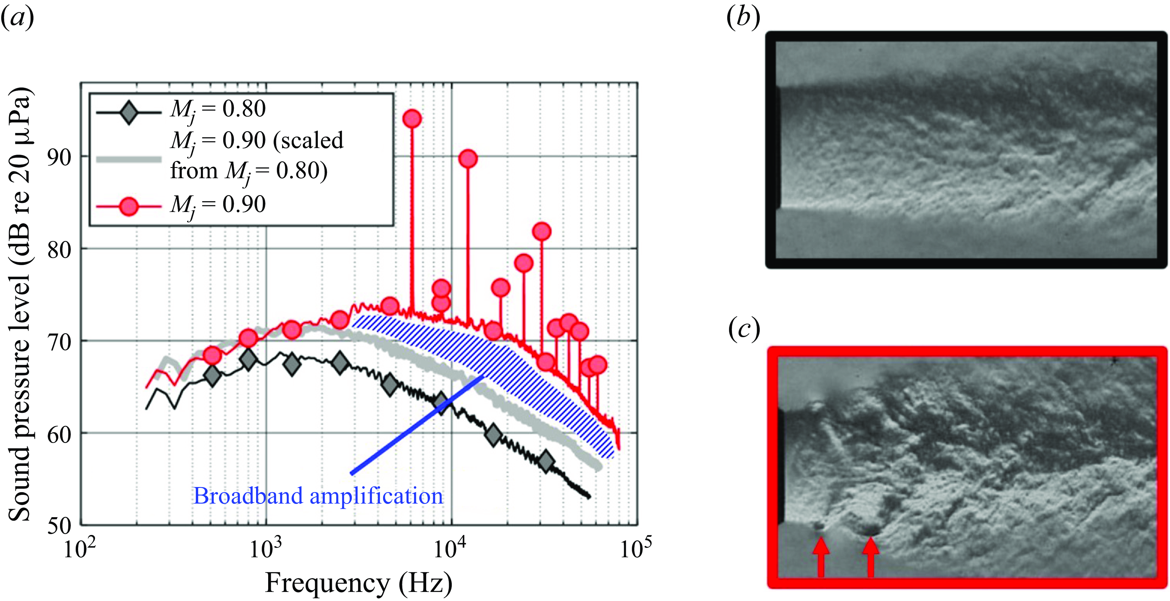
Figure 3 summarises data reported by Ramsey et al. (Reference Ramsey, Mayo, Karon, Funk and Ahuja2022b
). In figure 3(a), acoustic spectra measured in the jet’s far field at $\theta = 90^{\circ }$
from the jet axis are shown. The core and bypass streams were operated unheated and at the same total pressure. Thus, the flow from the nozzle was quite close to a single, round, unheated jet. At
$\theta = 90^{\circ }$
from the jet axis are shown. The core and bypass streams were operated unheated and at the same total pressure. Thus, the flow from the nozzle was quite close to a single, round, unheated jet. At $M_j = 0.80$
, a typical, broadband jet-noise spectrum is seen. By using well-established jet-noise scaling relations (Lighthill Reference Lighthill1952; Gaeta & Ahuja Reference Gaeta and Ahuja2003), this measured spectrum was then scaled to
$M_j = 0.80$
, a typical, broadband jet-noise spectrum is seen. By using well-established jet-noise scaling relations (Lighthill Reference Lighthill1952; Gaeta & Ahuja Reference Gaeta and Ahuja2003), this measured spectrum was then scaled to $M_j = 0.90$
, establishing an expected noise level for this higher
$M_j = 0.90$
, establishing an expected noise level for this higher $M_j$
(see the spectrum without data markers). However, the spectrum measured at
$M_j$
(see the spectrum without data markers). However, the spectrum measured at $M_j = 0.90$
shows much higher noise levels, containing discrete tones and a ‘broadband amplification’ of jet noise (e.g. see Ahuja & Blakney (Reference Ahuja and Blakney1985) for further details) that is emphasised with cross-hatching in the figure.
$M_j = 0.90$
shows much higher noise levels, containing discrete tones and a ‘broadband amplification’ of jet noise (e.g. see Ahuja & Blakney (Reference Ahuja and Blakney1985) for further details) that is emphasised with cross-hatching in the figure.
A schlieren image of the jet at $M_j = 0.80$
shown in figure 3(b) reflects a typical turbulent jet. A similar image obtained at
$M_j = 0.80$
shown in figure 3(b) reflects a typical turbulent jet. A similar image obtained at $M_j=0.90$
shown in figure 3(c) reveals that there were remarkable changes to the flow when the howling occurred. Namely, the Kelvin–Helmholtz instability waves (simply ‘instability waves’ hereafter) of the jet were excited as indicated with upward-facing arrows. The path integrated density gradients visualised by the schlieren technique must be interpreted with care. The reader should note that, as will be shown briefly in this paper (in § 3.5), the instability waves seen here are not axisymmetric about the jet axis. Ramsey et al. (Reference Ramsey, Mayo, Karon, Funk and Ahuja2022b
) did not explain why the howling was produced.
$M_j=0.90$
shown in figure 3(c) reveals that there were remarkable changes to the flow when the howling occurred. Namely, the Kelvin–Helmholtz instability waves (simply ‘instability waves’ hereafter) of the jet were excited as indicated with upward-facing arrows. The path integrated density gradients visualised by the schlieren technique must be interpreted with care. The reader should note that, as will be shown briefly in this paper (in § 3.5), the instability waves seen here are not axisymmetric about the jet axis. Ramsey et al. (Reference Ramsey, Mayo, Karon, Funk and Ahuja2022b
) did not explain why the howling was produced.
1.3. The cause of the howling
Aeroacoustic feedback phenomena (or just ‘feedback’) may occur in many different jet configurations. Classical examples involving a jet’s interaction with solid boundaries include edge-tone phenomena (e.g. see early works by Curle (Reference Curle1953); Powell (Reference Powell1953a )), impinging-jet resonances (e.g. see Powell Reference Powell1988; Tam & Ahuja Reference Tam and Ahuja1990; Henderson, Bridges & Wernet Reference Henderson, Bridges and Wernet2005) and resonances of ducted jets (e.g. see Bradshaw, Flintoff & Middleton Reference Bradshaw, Flintoff and Middleton1968; Ahuja et al. Reference Ahuja, Massey, Fleming, Tam and III1992; Tam, Ahuja & Jones Reference Tam, Ahuja and Jones1994; Samanta & Freund Reference Samanta and Freund2008; Topalian & Freund Reference Topalian and Freund2010). Only a selected few papers were referenced here due to a large volume of literature being available. The reader may reach more of this literature via review articles (e.g. see Ahuja Reference Ahuja2001 and Edgington-Mitchell Reference Edgington-Mitchell2019). Feedback phenomena typically give rise to high-amplitude acoustic tones and powerful flow oscillations, much like those shown in the previous subsection, and usually involve a flow instability which extracts energy from the motion of a fluid, the generation of sound which involves the instability in some fashion, and the subsequent coupling (i.e. ‘feedback’) of the generated sound back to the flow instability.
There are different ways in which feedback phenomena can involve or be modified by a ‘natural acoustic mode.’ Natural acoustic modes will be explained in greater detail shortly. For example, several prior authors (e.g. see Tam & Block Reference Tam and Block1978; Ahuja & Mendoza Reference Ahuja and Mendoza1995; and Yamouni, Sipp & Jacquin Reference Yamouni, Sipp and Jacquin2013) have studied the classical feedback phenomenon that occurs when flow passes over an open cavity. Generally, two different (and possibly interacting) resonance mechanisms can occur depending on the geometry and flow conditions: aeroacoustic feedback involving the instability waves in the shear layer above the open cavity and/or an excitation of a natural acoustic mode (or ‘acoustic resonance’) of the cavity. Another example is the ducted, screeching jets studied by Tam et al. (Reference Tam, Ahuja and Jones1994). When placed inside of a confining duct, jets that produce screech when unconfined may exhibit a different phenomenon; namely, a feedback phenomenon or coupling between the jet’s instability waves and the natural acoustic modes of the confining duct. Another notable example highlighting the important role of natural acoustic modes is the ‘Parker resonance’ (Parker Reference Parker1966), where a flow instability inside of a duct (vortex shedding in the wake of a flat plate) couples with a natural acoustic mode of the confining duct. The Parker resonance typically results in the flow instability locking on to the duct’s natural frequency, even if this frequency is slightly different from the instability’s characteristic frequency. Thus, this truly is a ‘feedback phenomenon’ involving a coupling of the instability with the natural acoustic mode.
We will show that the howling first reported by Ramsey et al. (Reference Ramsey, Karon, Funk and Ahuja2022b ) was the result of a feedback phenomenon inside the nozzle. Of the three scenarios described in the previous paragraph, the observed feedback phenomenon was most similar to the Parker resonance. For completeness, we note that a second, distinct type of feedback has been observed using the same nozzle when operated at different conditions (e.g. see Ramsey, Mayo & Ahuja Reference Ramsey, Mayo and Ahuja2023 and Ramsey Reference Ramsey2024). This second type of feedback is not discussed further in this paper.
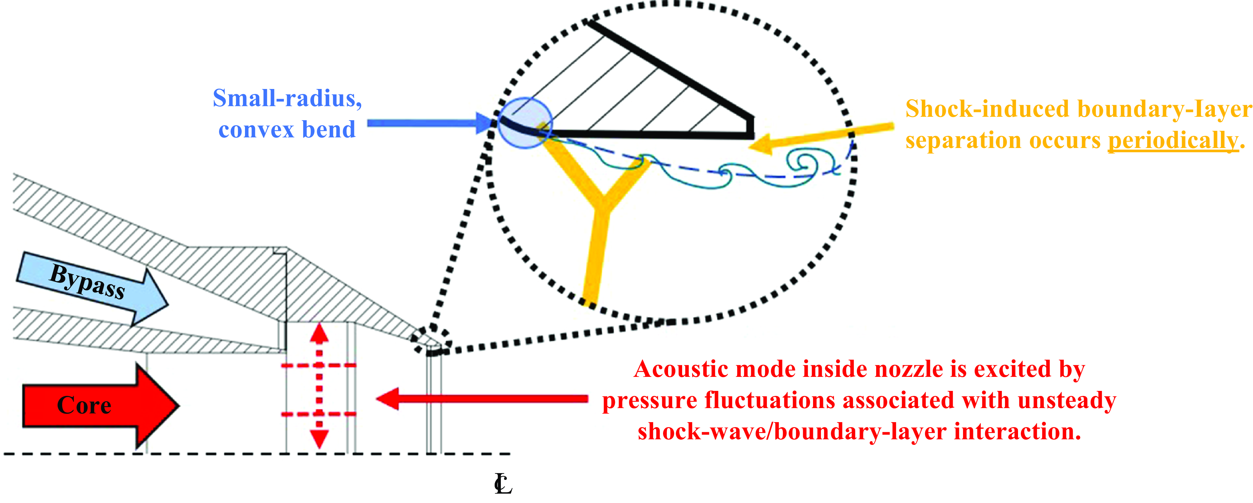
The feedback phenomenon studied in this paper involved the coupling between a periodic shock-wave/boundary-layer interaction (SWBLI) just upstream of the nozzle’s exit and a natural acoustic mode of the straight, cylindrical portion of the nozzle’s round mixing duct, as illustrated in figure 4. The natural acoustic modes relevant to the feedback phenomenon studied in this paper are the higher-order acoustic modes of the nozzle’s round mixing duct precisely at their ‘cut-on’ frequencies. Any unfamiliar reader should see classical acoustics textbooks such as Blackstock (Reference Blackstock2000) or § A.4 of Ramsey (Reference Ramsey2024). Cut-on frequencies are the frequencies at and above which the corresponding higher-order acoustic modes may propagate along the duct. Below this frequency, the higher-order modes are evanescent and their amplitudes decay exponentially with distance. Precisely at their respective cut-on frequencies, the higher-order acoustic modes have an important property: they possess zero axial group velocity ( $\partial \omega /\partial k = 0$
, where
$\partial \omega /\partial k = 0$
, where $\omega$
is the angular frequency and
$\omega$
is the angular frequency and $k$
is the axial wavenumber) such that they do not transport energy upstream or downstream. The duct is particularly prone to supporting aeroacoustic feedback phenomena at these frequencies, provided a flow instability occurs at a nearby frequency. Ahuja et al. (Reference Ahuja, Massey, Fleming, Tam and III1992) explained this concept too, and called them the ‘resonance waves’ of a round duct. In this paper, we simply call them ‘natural acoustic modes.’
$k$
is the axial wavenumber) such that they do not transport energy upstream or downstream. The duct is particularly prone to supporting aeroacoustic feedback phenomena at these frequencies, provided a flow instability occurs at a nearby frequency. Ahuja et al. (Reference Ahuja, Massey, Fleming, Tam and III1992) explained this concept too, and called them the ‘resonance waves’ of a round duct. In this paper, we simply call them ‘natural acoustic modes.’
Main components of the feedback phenomenon responsible for the howling. Coupling between the natural acoustic mode and the SWBLI not shown.
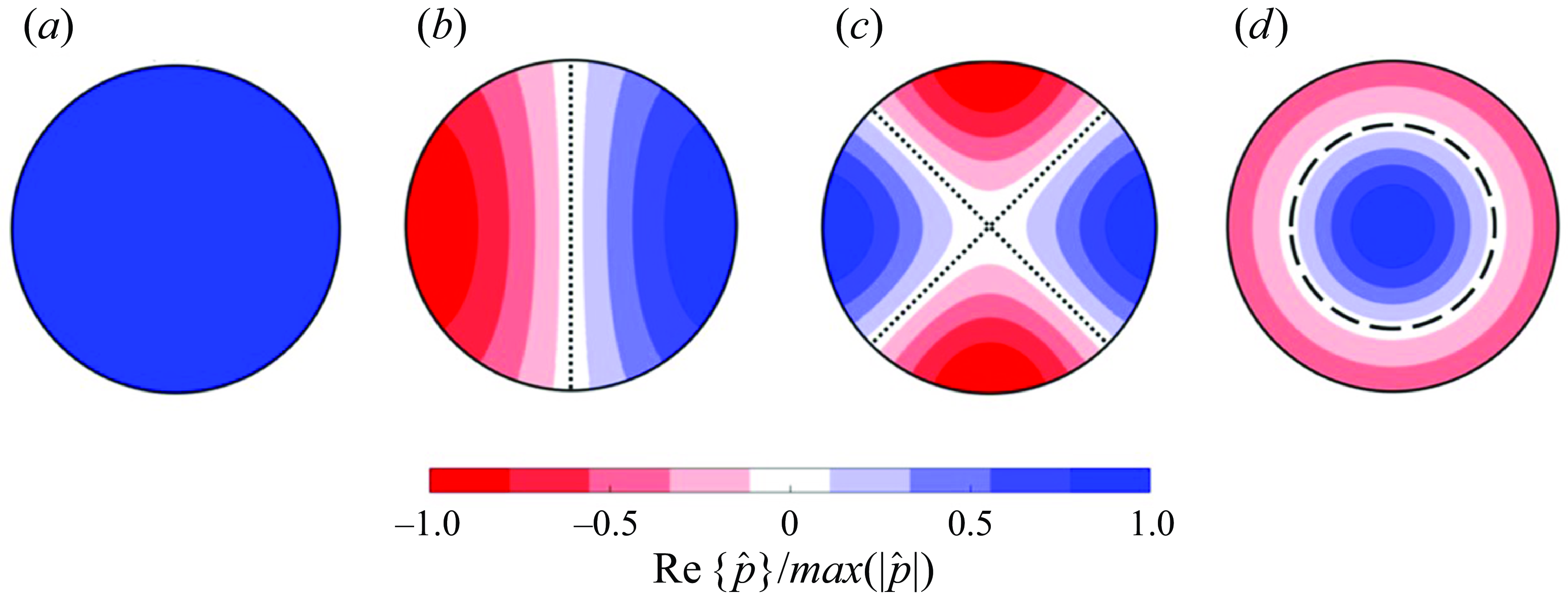
Due to the central importance of higher-order acoustic modes to the feedback phenomenon studied in this paper, the mode-numbering convention we adopted is illustrated in figure 5. The plane-wave mode is shown in figure 5(a). This mode involves pressure waves which appear as uniform fluctuations across the duct. Plane waves can propagate along the duct at any frequency, and thus have no cut-on frequency. Figure 5(b) shows the higher-order mode with the lowest cut-on frequency: the $(1,0)$
mode. Figure 5(c) shows the higher-order mode with the second-lowest cut-on frequency: the
$(1,0)$
mode. Figure 5(c) shows the higher-order mode with the second-lowest cut-on frequency: the $(2,0)$
mode. Finally, figure 5(d) shows the higher-order mode with the third-lowest cut-on frequency: the
$(2,0)$
mode. Finally, figure 5(d) shows the higher-order mode with the third-lowest cut-on frequency: the $(0,1)$
mode. The mode-numbering convention
$(0,1)$
mode. The mode-numbering convention $(m,n)$
followed here uses the azimuthal order
$(m,n)$
followed here uses the azimuthal order $m$
to mean the number of pressure nodal lines which run across the duct’s cross-section (see dotted lines in figures 5
b and 5
c) and the radial order
$m$
to mean the number of pressure nodal lines which run across the duct’s cross-section (see dotted lines in figures 5
b and 5
c) and the radial order $n$
to mean the ‘number of concentric nodal circles within the cross-section of the circular duct’ (Lympany & Ahuja Reference Lympany and Ahuja2020) (see dashed circle in figure 5
d). It will be shown that the SWBLI at the final nozzle’s exit predominantly coupled with the
$n$
to mean the ‘number of concentric nodal circles within the cross-section of the circular duct’ (Lympany & Ahuja Reference Lympany and Ahuja2020) (see dashed circle in figure 5
d). It will be shown that the SWBLI at the final nozzle’s exit predominantly coupled with the $(2,0)$
acoustic mode of the nozzle’s mixing duct at its cut-on frequency.
$(2,0)$
acoustic mode of the nozzle’s mixing duct at its cut-on frequency.
Acoustic pressure distributions associated with plane-wave mode and first three higher-order modes of a round duct: (a) plane-wave mode, (b) $(1,0)$
mode, (c)
$(1,0)$
mode, (c) $(2,0)$
mode and (d)
$(2,0)$
mode and (d) $(0,1)$
mode. Higher-order modes ordered with increasing cut-on frequency from left to right.
$(0,1)$
mode. Higher-order modes ordered with increasing cut-on frequency from left to right.
As will become clear when results are presented in this paper, the flow instability central to the feedback phenomenon (the SWBLI) was caused by a small-radius convex bend in the nozzle’s wall. It is noted that similar convex bends have been found in prior works to give rise to a broadband excess noise in internally mixed nozzles equipped with lobed mixers (e.g. see Garrison et al. Reference Garrison, Lyrintzis, Blaisdell and Dalton2005; Tester & Fisher Reference Tester and Fisher2006). However, there was no howling observed in these prior works. Internal, transonic flows have been known to give rise to unsteady SWBLIs for some time. A particularly notable discussion of this can be found in the work by Meier, Szumowski & Selerowicz (Reference Meier, Szumowski and Selerowicz1990), where a periodic SWBLI inside of a curved duct was described. This SWBLI bears some similarity to the one that underpins the howling studied here. Although they did not provide evidence of a coupling to an acoustic mode of the duct’s interior, the interested reader may wish to review their work as well. For completeness, it is also noted that convergent–divergent nozzles may exhibit a resonance related to a shock in the diverging section when operated at low pressure ratios (e.g. see Zaman et al. Reference Zaman, Dahl, Bencic and Loh2002). However, the nature of that resonance is quite different from the one studied here.
The remaining sections of this paper are as follows. In § 2, the experimental and computational methodologies used in this paper are outlined. In § 3, experimental and computational results are presented that give an understanding of the flow instability which is central to the howling (i.e. the periodic SWBLI inside the nozzle), as well as evidence of its coupling to the acoustic modes of the nozzle’s mixing duct. Then, in § 4, models are used to calculate the natural frequencies of the nozzle’s mixing duct, which include velocity and temperature differences between the core and bypass streams as well as the wake of the core-nozzle lip. Comparisons between these model calculations and experimental data are presented. Concluding remarks are given in § 5.
2. Methodology
2.1. Acoustic measurements
Far-field acoustic measurements were acquired in the GTRI Anechoic Jet Facility which has been well documented over the years (e.g. see Burrin, Dean & Tanna Reference Burrin, Dean and Tanna1974; Burrin & Tanna Reference Burrin and Tanna1979; Ahuja Reference Ahuja2003; Karon Reference Karon2016; Ramsey et al. Reference Ramsey, Karon, Funk and Ahuja2022a
; Karon & Ahuja Reference Karon and Ahuja2023). Acoustic pressures were measured using 1/4-inch free-field microphones positioned in the far field of the jet at a nominal 60 $D_e$
or greater. The microphones were either B&K model 4939 (paired with B&K 2669 pre-amplifiers connected to B&K Nexus 2960-A-0S4 signal-conditioning amplifiers) or PCB model 378C01. The facility was outfitted with both microphone types due to periodic upgrades to newer equipment. Regardless of which microphone model was used, the instrument’s complete frequency response was accounted for (e.g. see Ahuja (Reference Ahuja2003); Karon (Reference Karon2016) for a discussion of the various microphone frequency responses), thus eliminating any need to consider which microphone model was used to acquire which data in this paper. Microphone signals were sampled for 45 s (unless otherwise noted) at 204.8 kHz using NI PXIe-4499 modules. Power spectra were then calculated using Welch’s method (Welch Reference Welch1967) and Hanning-windowed data blocks with 50 % overlap. The number of points in each block was either
$D_e$
or greater. The microphones were either B&K model 4939 (paired with B&K 2669 pre-amplifiers connected to B&K Nexus 2960-A-0S4 signal-conditioning amplifiers) or PCB model 378C01. The facility was outfitted with both microphone types due to periodic upgrades to newer equipment. Regardless of which microphone model was used, the instrument’s complete frequency response was accounted for (e.g. see Ahuja (Reference Ahuja2003); Karon (Reference Karon2016) for a discussion of the various microphone frequency responses), thus eliminating any need to consider which microphone model was used to acquire which data in this paper. Microphone signals were sampled for 45 s (unless otherwise noted) at 204.8 kHz using NI PXIe-4499 modules. Power spectra were then calculated using Welch’s method (Welch Reference Welch1967) and Hanning-windowed data blocks with 50 % overlap. The number of points in each block was either $N_{DFT} = 6400$
(yielding
$N_{DFT} = 6400$
(yielding $\Delta f = 32$
Hz) or
$\Delta f = 32$
Hz) or $N_{DFT} = 81920$
(yielding
$N_{DFT} = 81920$
(yielding $\Delta f = 2.5$
Hz). Any frequency bins in the acoustic spectra that were within 12 dB of the spectral noise floor measured with the chamber entry doors closed and no flow supplied to the facility were removed before plotting, ensuring an extremely high signal-to-noise ratio. The power spectra were then made lossless by applying a standard correction for atmospheric attenuation (ANSI S1.26–1995 1995) from the centre of the nozzle exit to the microphone.
$\Delta f = 2.5$
Hz). Any frequency bins in the acoustic spectra that were within 12 dB of the spectral noise floor measured with the chamber entry doors closed and no flow supplied to the facility were removed before plotting, ensuring an extremely high signal-to-noise ratio. The power spectra were then made lossless by applying a standard correction for atmospheric attenuation (ANSI S1.26–1995 1995) from the centre of the nozzle exit to the microphone.
2.2. Schlieren flow visualisations
Flow measurements were acquired in a separate facility: the GTRI Flow-Diagnostics Facility (Burrin & Tanna Reference Burrin and Tanna1979). The facility’s Z-type schlieren system was used. The Z-type schlieren system utilised a continuously operating arc lamp as the light source, a knife-edge cutoff oriented parallel to the jet axis (showing transverse density gradients in the jet) and a Vision Research Phantom V2512 high-speed camera to capture the images.
2.3. Numerical simulations
A cross-sectional view of the computational grid used is shown in figure 6. Any regions in the images showing the grid that appear solid black reflect a relatively fine grid being used there. The computational grid was constructed directly from model initial graphics exchange specification files of the nozzle with truncated 1.27-millimetre trailing-edge thickness on the core- and final-nozzle trailing edges. The grid was constructed using HeldenMesh with at least 25 prism layers in the region of attached boundary-layer fluid (targeted at the nozzle trailing edges). Tetrahedral cells were used in the internal passages and the external shear layer. Sourcing in the volume region ensured a smooth transition from the prisms to the tetrahedral cells with about 15 cells across the trailing edges and Taylor-scale resolution out to $x/D_e$
= 15. Iterative, hand-crafted grid refinement was used to ensure a smooth transition from this finely resolved region to a coarser grid further downstream, thus avoiding spurious acoustic source mechanisms and grid reflections. Grid refinement also included an acoustic buffer outside the jet/ambient shear layer for eventual coupling with a Ffowcs Williams-Hawkings surface, although no acoustic predictions are reported herein.
$x/D_e$
= 15. Iterative, hand-crafted grid refinement was used to ensure a smooth transition from this finely resolved region to a coarser grid further downstream, thus avoiding spurious acoustic source mechanisms and grid reflections. Grid refinement also included an acoustic buffer outside the jet/ambient shear layer for eventual coupling with a Ffowcs Williams-Hawkings surface, although no acoustic predictions are reported herein.
Cross-sectional views of the computational grid used: (a) view of computational domain with nozzle coupled to plenum chambers on left and (b,c) detailed view of the grid inside the nozzle near final-nozzle exit. Colour in (b,c) shows time-averaged local Mach number for $M_j = 0.90$
, unheated operating condition.
$M_j = 0.90$
, unheated operating condition.

Reynolds-averaged Navier–Stokes (RANS) and hybrid RANS/large-eddy simulations (HRLES) were performed using the NASA FUN3D framework (Anderson 2022). This is a node-centred, finite-volume scheme with nominally second-order spatial discretisation. The RANS simulations used Menter’s two-equation eddy viscosity model (Menter, Reference Menter1994) for closure. Where HRLES was used, the sub-grid-scale Reynolds stresses were modelled using a one-equation model given by Kim & Menon (Reference Kim and Menon1995) in LES solution regions and the Menter’s model was used in the RANS solution regions. Generally, the solver switches from LES to RANS in regions where the Kolmogorov length scale is small and LES grows increasingly costly (e.g. near the solid walls of the nozzle). As discussed by Lynch & Smith (Reference Lynch and Smith2008), the constants used in the underlying turbulence models were blended between LES and RANS solution regions using the original blending function by Menter (Reference Menter1994).
HRLES results were obtained as the final result of a three-step simulation campaign, which included a grid-refinement study as outlined here. First, a RANS problem was solved. During this stage, grid-refinement studies were performed to achieve a practical balance between the competing requirements of resolving flow physics and computational cost. The grid resolution was iteratively increased until the core nozzle’s wake and the final jet’s shear layer were adequately resolved. Simulation data from this phase were used to inform a semi-empirical model of the turbulent kinetic energy spectrum. This semi-empirical model was then used to select a minimum resolution (versus axial distance) to resolve at least 80 % of the local turbulent kinetic energy. Then, further grid studies were performed to achieve relatively smooth transition from the resolved portions of the domain to the background grid for avoidance of artefacts. Second, with the refined grid, the RANS result was used as the initial condition for a temporally coarse HRLES simulation where the startup transient was allowed to convect downstream past $x/D_e \approx$
20. Initial HRLES results were used to check for grid adequacy. It was necessary to increase the radial extent of the high-resolution grid in the final jet’s shear layer to capture instability waves, which are not present in RANS simulations. Finally, the temporally coarse HRLES result was then used as the initial condition for a high-resolution HRLES simulation resolving Strouhal numbers (based on
$x/D_e \approx$
20. Initial HRLES results were used to check for grid adequacy. It was necessary to increase the radial extent of the high-resolution grid in the final jet’s shear layer to capture instability waves, which are not present in RANS simulations. Finally, the temporally coarse HRLES result was then used as the initial condition for a high-resolution HRLES simulation resolving Strouhal numbers (based on $D_e$
and
$D_e$
and $U_j$
) up to 2.0 with 25x over sampling. Time stepping was done using optimised second-order backward differencing with 15–20 sub-iterations per physical time step, which was adequate to drive residuals down by at least 5 orders of magnitude at each time step. A low-dissipation variant of the Roe approximate Riemann solver (Nishikawa & Liu Reference Nishikawa and Liu2018) was used to account for the inviscid interaction of adjacent fluid cells via the flux through their shared interface, here with emphasis on accurately capturing the acoustic fluctuations outside the jet/ambient shear layer.
$U_j$
) up to 2.0 with 25x over sampling. Time stepping was done using optimised second-order backward differencing with 15–20 sub-iterations per physical time step, which was adequate to drive residuals down by at least 5 orders of magnitude at each time step. A low-dissipation variant of the Roe approximate Riemann solver (Nishikawa & Liu Reference Nishikawa and Liu2018) was used to account for the inviscid interaction of adjacent fluid cells via the flux through their shared interface, here with emphasis on accurately capturing the acoustic fluctuations outside the jet/ambient shear layer.
3. Experimental and computational results
There are several subsections of results appearing below. First, in § 3.1, experimental flow visualisations reveal an unusual flow instability was present when the howling occurred. Then, in § 3.2 and § 3.3, computational results provide insight into the cause and nature of this flow instability and show that it can couple with a higher-order acoustic mode of the nozzle’s mixing duct. Then, in § 3.4 trends in experimental acoustic data characterise the howling frequency and amplitude, with preliminary estimates of the cut-on frequencies of the higher-order acoustic modes of the nozzle’s mixing duct provided for comparison. Finally, § 3.5 contains experimental flow data that further indicate the flow instability coupled with a particular natural acoustic mode of the nozzle’s mixing duct.
3.1. Experimental measurements of periodic separation
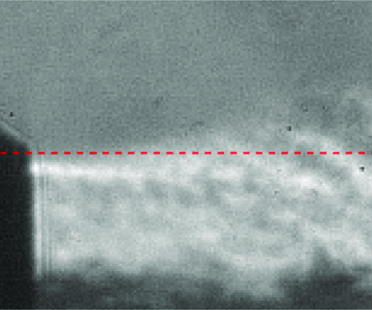
A series of time-resolved schlieren snapshots is shown in figure 7. The snapshots were acquired with the $L_e/D_e = 0.7$
mixing-duct length operated at
$L_e/D_e = 0.7$
mixing-duct length operated at $M_j = 0.90$
with both streams unheated – an operating condition at which the nozzle produced a powerful howling. A close-up view of the flow at and just downstream of the nozzle exit is shown. The dark shape on the left-hand side of each snapshot at
$M_j = 0.90$
with both streams unheated – an operating condition at which the nozzle produced a powerful howling. A close-up view of the flow at and just downstream of the nozzle exit is shown. The dark shape on the left-hand side of each snapshot at $x \lt 0$
is the silhouette of the final nozzle. The high spatial resolution of these snapshots is evident upon inspection of the axes against which they are plotted: the snapshots span less than 0.1
$x \lt 0$
is the silhouette of the final nozzle. The high spatial resolution of these snapshots is evident upon inspection of the axes against which they are plotted: the snapshots span less than 0.1 $D_e$
in the transverse and axial directions. Within all the snapshots, a horizontal, dashed line located at the lipline of the nozzle (
$D_e$
in the transverse and axial directions. Within all the snapshots, a horizontal, dashed line located at the lipline of the nozzle ( $y = 0.5D_e$
) is shown for visual reference. The images were acquired at a nominal sampling rate of 270 kHz (the ‘actual’ sampling rate reported by the camera’s control software was about 270.968 kHz). A segment from the schlieren recording is provided as Supplementary Movie 1, which shows a larger field of view than the still snapshots printed in the figure. The still snapshots are intended to recreate and emphasise the key oscillations visible in the movie. Each snapshot is assigned a number that is printed above it, with an increase in the number representing a forward passage of time.
$y = 0.5D_e$
) is shown for visual reference. The images were acquired at a nominal sampling rate of 270 kHz (the ‘actual’ sampling rate reported by the camera’s control software was about 270.968 kHz). A segment from the schlieren recording is provided as Supplementary Movie 1, which shows a larger field of view than the still snapshots printed in the figure. The still snapshots are intended to recreate and emphasise the key oscillations visible in the movie. Each snapshot is assigned a number that is printed above it, with an increase in the number representing a forward passage of time.
One cycle of separation/reattachment shown by down-sampled series of time-resolved schlieren images (every fourth image) with $L_e/D_e$
= 0.7,
$L_e/D_e$
= 0.7, $M_j$
= 0.90, unheated. Flow is left to right. A segment of the schlieren recording is available for playback (see supplementary movie 1).
$M_j$
= 0.90, unheated. Flow is left to right. A segment of the schlieren recording is available for playback (see supplementary movie 1).
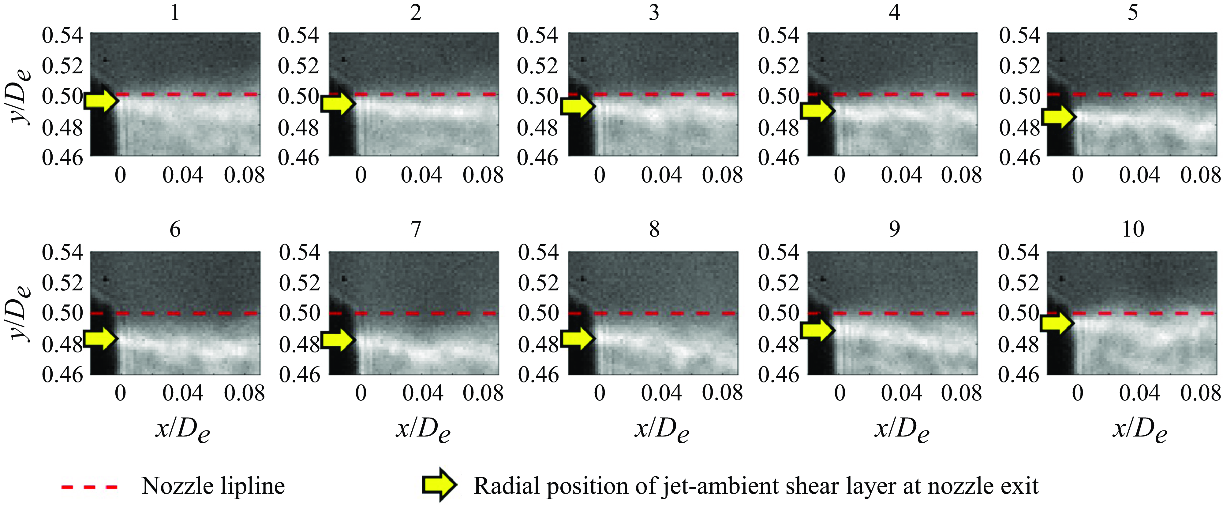
In snapshot 1 of figure 7, a bright white region is visible just below the nozzle lipline. This is the jet/ambient shear layer where transverse density gradients were present because the jet was unheated. The approximate location of the jet/ambient shear layer at the nozzle-exit plane is indicated with a rightward-pointing arrow in each snapshot. By comparing the relative position of the arrow and the dashed line across the snapshots, the shear layer’s oscillation in time is visible. Snapshots 1–6 show the shear layer moving away from the nozzle lip, while snapshots 7–10 show the shear layer returning to the nozzle lip. This is clear evidence that, when the howling occurred, the boundary layer just upstream of the nozzle’s exit periodically separated and reattached. At $M_j = 0.80$
and
$M_j = 0.80$
and $M_j = 1.00$
, similar visualisations were obtained with an unheated and a heated core stream, which are not shown for brevity. These operating conditions did not produce any howling, and no periodic separation was visible in the visualisations.
$M_j = 1.00$
, similar visualisations were obtained with an unheated and a heated core stream, which are not shown for brevity. These operating conditions did not produce any howling, and no periodic separation was visible in the visualisations.
A spectral proper orthogonal decomposition (SPOD) of the fluctuations in the schlieren images was conducted using the open-source MATLAB code documented by Towne, Schmidt & Colonius (Reference Towne, Schmidt and Colonius2018) (available at https://github.com/SpectralPOD/spod_matlab). Welch’s method of spectral estimation (Welch Reference Welch1967) was used with $2048$
-image, Hanning-windowed blocks with 50 % overlap across
$2048$
-image, Hanning-windowed blocks with 50 % overlap across $8192$
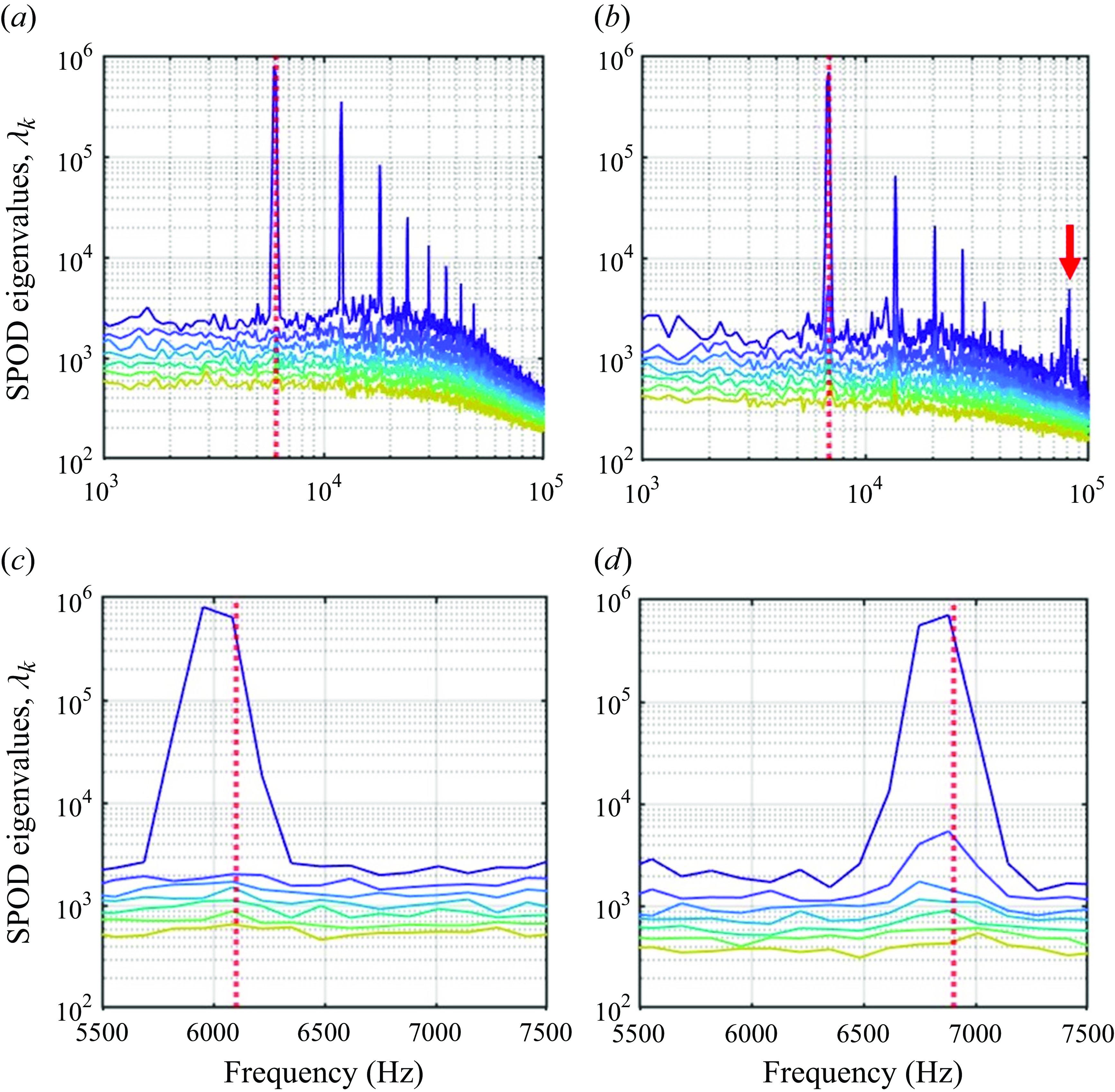
total images (corresponding to a duration of approximately 0.03 s). Figure 8(a) shows all seven SPOD eigenvalue spectra obtained from analysing the schlieren video acquired with the core stream unheated. At the nominal frequency of the measured, fundamental acoustic tone (indicated by the vertical, dotted line), the leading-order SPOD mode’s eigenvalue spectrum contains a peak which indicates organised, high-amplitude oscillations at that frequency. As will be shown below in figure 9, the SPOD mode corresponding to this peak in the spectrum was inspected and confirmed to represent the periodic separation visible in the schlieren recording. As expected, harmonics of the fundamental tone are present as well.
$8192$
total images (corresponding to a duration of approximately 0.03 s). Figure 8(a) shows all seven SPOD eigenvalue spectra obtained from analysing the schlieren video acquired with the core stream unheated. At the nominal frequency of the measured, fundamental acoustic tone (indicated by the vertical, dotted line), the leading-order SPOD mode’s eigenvalue spectrum contains a peak which indicates organised, high-amplitude oscillations at that frequency. As will be shown below in figure 9, the SPOD mode corresponding to this peak in the spectrum was inspected and confirmed to represent the periodic separation visible in the schlieren recording. As expected, harmonics of the fundamental tone are present as well.
SPOD eigenvalue spectra obtained from schlieren with $L_e/D_e = 0.7$
,
$L_e/D_e = 0.7$
, $M_j = 0.90$
: (a,c) unheated and (b,d) heated core stream (
$M_j = 0.90$
: (a,c) unheated and (b,d) heated core stream ( $T_{t1} \approx 533$
K,
$T_{t1} \approx 533$
K, $TTR_1 \approx 1.85$
). (c,d) Show same spectra as (a,b) over limited frequency range. Nominal, measured frequency of fundamental acoustic tones plotted as vertical, dotted lines.
$TTR_1 \approx 1.85$
). (c,d) Show same spectra as (a,b) over limited frequency range. Nominal, measured frequency of fundamental acoustic tones plotted as vertical, dotted lines.
Leading-order SPOD modes obtained from measured schlieren with $L_e/D_e = 0.7$
,
$L_e/D_e = 0.7$
, $M_j = 0.90$
with (a) flow unheated and (b,c) heated core stream (
$M_j = 0.90$
with (a) flow unheated and (b,c) heated core stream ( $T_{t1} \approx 533$
K,
$T_{t1} \approx 533$
K, $TTR_1 \approx 1.85$
). In each panel the frequency of the SPOD mode is shown in the top, left-hand corner and lipline of final nozzle shown as a white, dashed line. Normalised real part shown for arbitrary phase. Flow is left to right.
$TTR_1 \approx 1.85$
). In each panel the frequency of the SPOD mode is shown in the top, left-hand corner and lipline of final nozzle shown as a white, dashed line. Normalised real part shown for arbitrary phase. Flow is left to right.
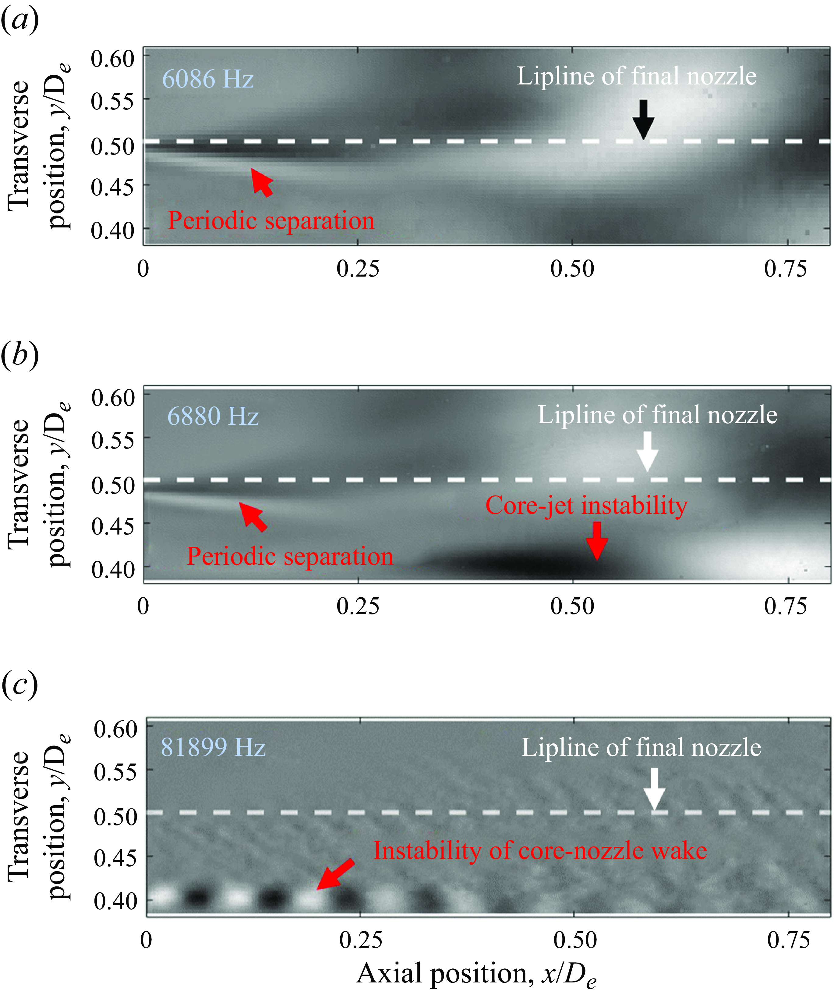
Figure 8(b) shows the eigenvalue spectra obtained by analysing a similar schlieren recording acquired with the core stream heated to $T_{t1} \approx 533$
K (
$T_{t1} \approx 533$
K ( $TTR_1 \approx 1.85$
). A segment from this schlieren recording is provided as Supplementary Movie 2. The separation frequency evident from the schlieren and the nominal frequency of the fundamental tone from acoustic measurements (indicated by a vertical dotted line) match with the core stream heated as well. The eigenvalue spectra are quite similar to those with the core stream unheated; however, a high-frequency feature is indicated by a downward-pointing arrow at a relatively high frequency. This is the signature of unsteady flow features in the wake of the core-nozzle lip as they exit the final nozzle. This conclusion was drawn by inspecting the leading-order SPOD mode at this frequency, which will be shown below in figure 9. Again, the instability in the wake of the core-nozzle lip is not discussed further because it is of too high a frequency to cause the howling studied here.
$TTR_1 \approx 1.85$
). A segment from this schlieren recording is provided as Supplementary Movie 2. The separation frequency evident from the schlieren and the nominal frequency of the fundamental tone from acoustic measurements (indicated by a vertical dotted line) match with the core stream heated as well. The eigenvalue spectra are quite similar to those with the core stream unheated; however, a high-frequency feature is indicated by a downward-pointing arrow at a relatively high frequency. This is the signature of unsteady flow features in the wake of the core-nozzle lip as they exit the final nozzle. This conclusion was drawn by inspecting the leading-order SPOD mode at this frequency, which will be shown below in figure 9. Again, the instability in the wake of the core-nozzle lip is not discussed further because it is of too high a frequency to cause the howling studied here.
Close-up views of the fundamental peaks in the SPOD eigenvalue spectra are shown in figures 8(c) and 8(d), emphasising the excellent agreement between the nominal frequencies of the acoustic tones and the periodic separation. The peaks in the leading-order eigenvalue spectra (the top-most spectra in figures 8 c and 8 d) are more than two orders of magnitude greater than the spectra appearing beneath them. This indicates that the fluctuations in the video at the frequency of the fundamental acoustic tone are dominated by an orderly flow feature: the signature of the periodic separation. The excellent agreement between the acoustic tone’s frequency and the periodic separation’s frequency suggests a feedback phenomenon involving the flow instability responsible for the periodic separation caused the observed howling. Again, the nature of this flow instability is made clear in the following two subsections.
For completeness, salient leading-order SPOD modes associated with the schlieren recordings are shown in figure 9. In each of the three panels, the lipline of the final nozzle is shown as a horizontal, white dashed line and the corresponding frequency is printed on the top, left-hand corner. The SPOD mode shown in figure 9(a) corresponds to the fundamental frequency present in the schlieren with unheated flow. Alternating dark and bright regions can be seen on the far left near $x = 0$
and just below the lipline of the final nozzle (see red arrow). This is the signature of the periodic separation at the nozzle exit. Figure 9(b) shows a similar signature of the periodic separation, but also reveals a signature of the core-jet instability waves when the core stream is heated and there is substantial difference between the two streams’ jet velocities. Because similar phenomena were observed with the flow unheated, this instability is believed to occur as a passive response of the core jet to the fluctuations associated with the howling. The core-jet instability is not discussed further in this paper. For completeness, figure 9(c) shows the high-frequency signature of what is believed to be vortex shedding from the core-nozzle lip. This vortex shedding and the noise it produces were studied by Ramsey et al. (Reference Ramsey, Larisch and Ahuja2025). The vortex-shedding frequency is an order of magnitude higher than the howling frequency and is thus not needed to explain the observed howling.
$x = 0$
and just below the lipline of the final nozzle (see red arrow). This is the signature of the periodic separation at the nozzle exit. Figure 9(b) shows a similar signature of the periodic separation, but also reveals a signature of the core-jet instability waves when the core stream is heated and there is substantial difference between the two streams’ jet velocities. Because similar phenomena were observed with the flow unheated, this instability is believed to occur as a passive response of the core jet to the fluctuations associated with the howling. The core-jet instability is not discussed further in this paper. For completeness, figure 9(c) shows the high-frequency signature of what is believed to be vortex shedding from the core-nozzle lip. This vortex shedding and the noise it produces were studied by Ramsey et al. (Reference Ramsey, Larisch and Ahuja2025). The vortex-shedding frequency is an order of magnitude higher than the howling frequency and is thus not needed to explain the observed howling.
3.2. Evidence that the boundary-layer separation is shock induced
RANS simulation results are shown in figure 10. In figure 10(a), a typical local-Mach-number distribution is shown at and just upstream of the final-nozzle exit for the $L_e/D_e$
= 0.7 mixing-duct length operated at
$L_e/D_e$
= 0.7 mixing-duct length operated at $M_j$
= 0.90, unheated, which produced a powerful howling in the experiments. The white space in the centre, top portion of this image is the cross-section of the final nozzle, with the flow from left to right as indicated by the streamlines. A small-radius bend existed along the final-nozzle wall between its converging and final straight sections and, from this Mach-number distribution, it is evident that there was localised supersonic flow in this region. This is very similar to the locally supersonic flow found by prior researchers studying internally mixed nozzles with a small-radius, convex bend in the nozzle wall (e.g. see Garrison et al. Reference Garrison, Lyrintzis, Blaisdell and Dalton2005; Wright, Blaisdell & Lyrintzis Reference Wright, Blaisdell and Lyrintzis2006; Kube-McDowell, Lyrintzis & Blaisdell Reference Kube-McDowell, Lyrintzis and Blaisdell2010). The supersonic flow was necessarily over-expanded because the stagnation-to-ambient pressure ratio was subcritical. Therefore, to eventually reach the ambient pressure outside the nozzle, the supersonic region was terminated by a shock wave. The right half of the ‘Mach = 1 contour’ called out in the image indicates the location of a shock. The left half of this contour simply represents the locus of physical points where gas flowing through the supersonic region reached sonic speed. The inlaid view emphasises the lambda-shock structure, indicating that shock-induced boundary-layer separation occurred. The upstream leg of the lambda-shock structure is not made visible by the Mach = 1 contour because it was an oblique shock that turned the flow away from the wall but did not bring the flow back down to subsonic speeds.
$M_j$
= 0.90, unheated, which produced a powerful howling in the experiments. The white space in the centre, top portion of this image is the cross-section of the final nozzle, with the flow from left to right as indicated by the streamlines. A small-radius bend existed along the final-nozzle wall between its converging and final straight sections and, from this Mach-number distribution, it is evident that there was localised supersonic flow in this region. This is very similar to the locally supersonic flow found by prior researchers studying internally mixed nozzles with a small-radius, convex bend in the nozzle wall (e.g. see Garrison et al. Reference Garrison, Lyrintzis, Blaisdell and Dalton2005; Wright, Blaisdell & Lyrintzis Reference Wright, Blaisdell and Lyrintzis2006; Kube-McDowell, Lyrintzis & Blaisdell Reference Kube-McDowell, Lyrintzis and Blaisdell2010). The supersonic flow was necessarily over-expanded because the stagnation-to-ambient pressure ratio was subcritical. Therefore, to eventually reach the ambient pressure outside the nozzle, the supersonic region was terminated by a shock wave. The right half of the ‘Mach = 1 contour’ called out in the image indicates the location of a shock. The left half of this contour simply represents the locus of physical points where gas flowing through the supersonic region reached sonic speed. The inlaid view emphasises the lambda-shock structure, indicating that shock-induced boundary-layer separation occurred. The upstream leg of the lambda-shock structure is not made visible by the Mach = 1 contour because it was an oblique shock that turned the flow away from the wall but did not bring the flow back down to subsonic speeds.
RANS results for $L_e/D_e$
= 0.7, unheated: (a) map of local Mach number at
$L_e/D_e$
= 0.7, unheated: (a) map of local Mach number at $M_j$
= 0.90 and (b) maximum local Mach number inside nozzle across a range of
$M_j$
= 0.90 and (b) maximum local Mach number inside nozzle across a range of $M_j$
.
$M_j$
.
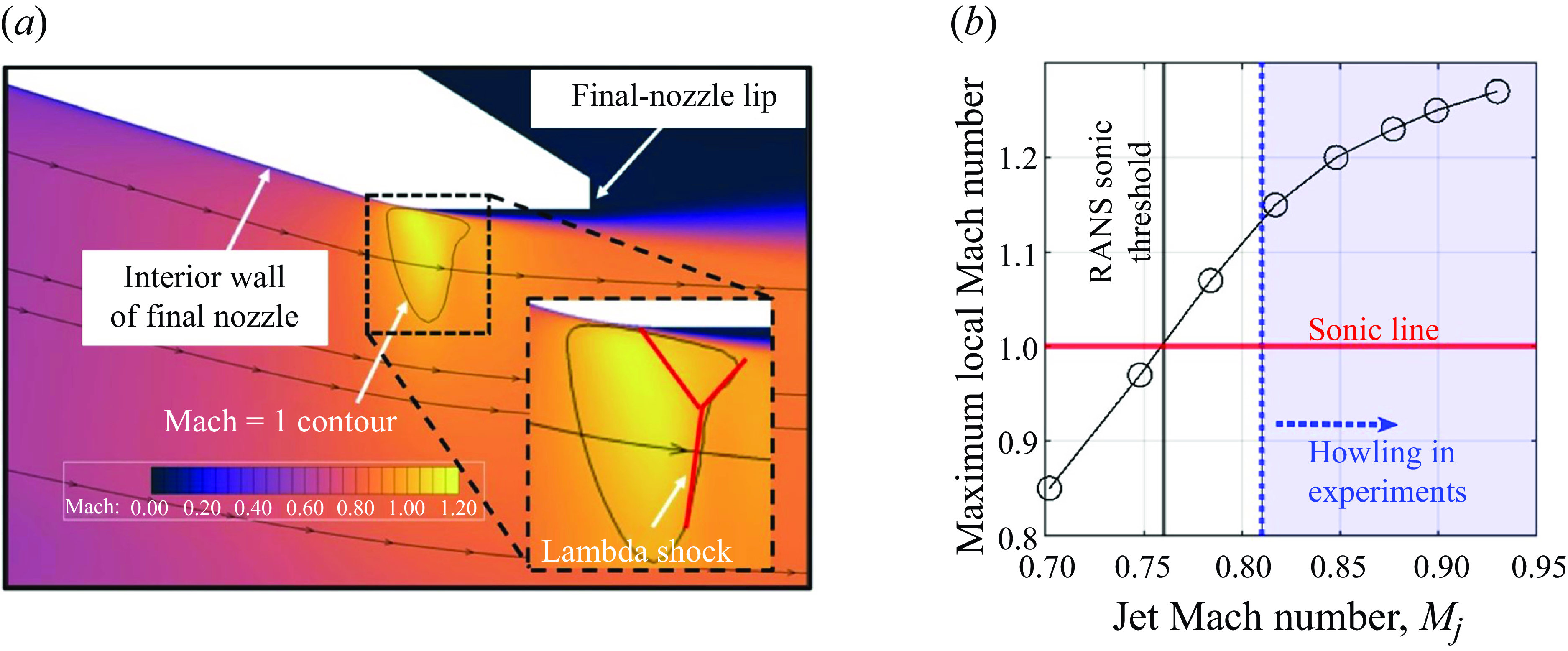
A series of RANS simulations were conducted at several $M_j$
between 0.70 and 0.93, using the same
$M_j$
between 0.70 and 0.93, using the same $L_e/D_e = 0.7$
mixing-duct length and with unheated flow. The maximum local Mach number inside the nozzle was extracted from each simulation, and the results are summarised in figure 10(b). The specified
$L_e/D_e = 0.7$
mixing-duct length and with unheated flow. The maximum local Mach number inside the nozzle was extracted from each simulation, and the results are summarised in figure 10(b). The specified $M_j$
is listed on the horizontal axis and the resulting maximum local Mach number is indicated on the vertical axis. A horizontal ‘sonic line’ is plotted at unity Mach number for reference. The RANS simulations suggested that a region of supersonic flow exists inside the nozzle above
$M_j$
is listed on the horizontal axis and the resulting maximum local Mach number is indicated on the vertical axis. A horizontal ‘sonic line’ is plotted at unity Mach number for reference. The RANS simulations suggested that a region of supersonic flow exists inside the nozzle above $M_j$
between 0.75 and 0.78. A linear interpolation suggested
$M_j$
between 0.75 and 0.78. A linear interpolation suggested $M_j = 0.76$
and is indicated by the solid, vertical line: the ‘RANS sonic threshold.’ If shock-induced boundary-layer separation were necessary for the howling to occur, the
$M_j = 0.76$
and is indicated by the solid, vertical line: the ‘RANS sonic threshold.’ If shock-induced boundary-layer separation were necessary for the howling to occur, the $M_j$
above which howling ensued in experiments should be above the RANS sonic threshold. Experimental data (to be discussed in § 3.4) indicated that howling may occur for
$M_j$
above which howling ensued in experiments should be above the RANS sonic threshold. Experimental data (to be discussed in § 3.4) indicated that howling may occur for $M_j$
as low as 0.81. This is indicated in figure 10(b) by the shaded region to the right of the vertical, dotted line. These results show that, when howling occurred in the experiments, the computations indicate a region of supersonic flow exists inside the nozzle. Supersonic flow inside the nozzle (and thus a shock inside the nozzle) was evidently necessary for the howling to occur.
$M_j$
as low as 0.81. This is indicated in figure 10(b) by the shaded region to the right of the vertical, dotted line. These results show that, when howling occurred in the experiments, the computations indicate a region of supersonic flow exists inside the nozzle. Supersonic flow inside the nozzle (and thus a shock inside the nozzle) was evidently necessary for the howling to occur.
One may wonder why the howling does not occur precisely at the RANS sonic threshold. This is understood as follows. A shock’s presence inside the nozzle is a necessary but not sufficient condition for shock-induced boundary-layer separation. The shock must not only be present but also strong enough (i.e. it must bring about a sufficiently large adverse pressure gradient) to separate the boundary layer upon its interaction with it. This is consistent with our observations that the lowest $M_j$
that produced howling in experiments (
$M_j$
that produced howling in experiments ( $M_j$
= 0.81, as noted in the previous paragraph) is higher than the RANS sonic threshold. A variety of indicators for the onset of flow instability were used for sensible judgement of the RANS results, suggesting that flow instability occurs for
$M_j$
= 0.81, as noted in the previous paragraph) is higher than the RANS sonic threshold. A variety of indicators for the onset of flow instability were used for sensible judgement of the RANS results, suggesting that flow instability occurs for $M_j \geqslant 0.85$
. Therefore, we cautiously note that the RANS simulations themselves indicated a flow instability did not occur precisely at the RANS sonic threshold but rather at higher
$M_j \geqslant 0.85$
. Therefore, we cautiously note that the RANS simulations themselves indicated a flow instability did not occur precisely at the RANS sonic threshold but rather at higher $M_j$
. Grid-refinement studies were not performed but would likely fine tune this finding. Detecting the onset of flow instability using RANS is imprecise, and we avoid weighing such indicators too heavily.
$M_j$
. Grid-refinement studies were not performed but would likely fine tune this finding. Detecting the onset of flow instability using RANS is imprecise, and we avoid weighing such indicators too heavily.
3.3. Explaining why the boundary-layer separation is periodic
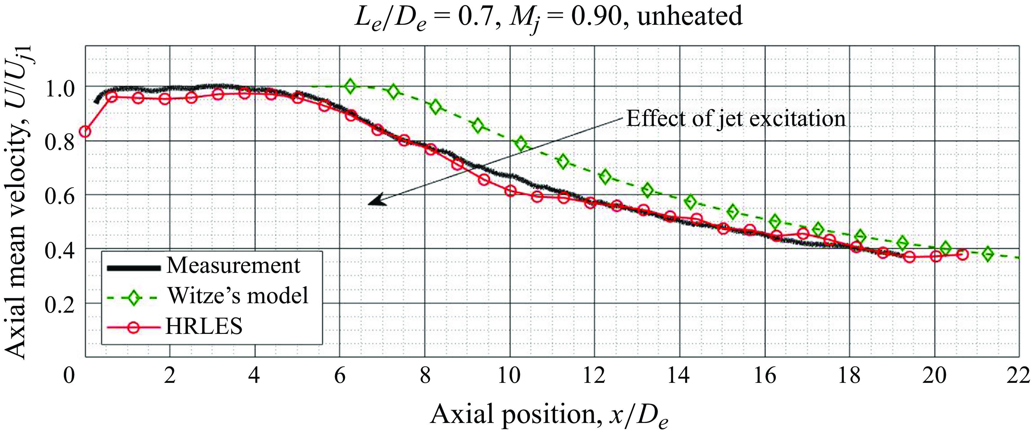
HRLES results are presented here for $L_e/D_e = 0.7$
,
$L_e/D_e = 0.7$
, $M_j = 0.90$
with the flow unheated. In figure 11, the mean-velocity distribution along the jet’s centreline obtained from the HRLES at
$M_j = 0.90$
with the flow unheated. In figure 11, the mean-velocity distribution along the jet’s centreline obtained from the HRLES at $M_j = 0.90$
is shown to have close agreement with the ensemble-averaged particle-image velocimetry (PIV) measurements first reported by Ramsey et al. (Reference Ramsey, Mayo, Karon, Funk and Ahuja2022b
). Witze (Reference Witze1974) provided a model for a single, round jet (approximately what the nozzle produces at unheated operating conditions with both streams at the same pressure ratio) that was included in the figure to emphasise the shortening of the potential core of the jet that occurred along with the howling. This is a typical effect of jet excitation (e.g. see Ahuja, Lepicovsky & Burrin (Reference Ahuja, Lepicovsky and Burrin1982)). The agreement between the HRLES results and experimental data inspired confidence that the jet excitation present in the experiments was captured by the simulation.
$M_j = 0.90$
is shown to have close agreement with the ensemble-averaged particle-image velocimetry (PIV) measurements first reported by Ramsey et al. (Reference Ramsey, Mayo, Karon, Funk and Ahuja2022b
). Witze (Reference Witze1974) provided a model for a single, round jet (approximately what the nozzle produces at unheated operating conditions with both streams at the same pressure ratio) that was included in the figure to emphasise the shortening of the potential core of the jet that occurred along with the howling. This is a typical effect of jet excitation (e.g. see Ahuja, Lepicovsky & Burrin (Reference Ahuja, Lepicovsky and Burrin1982)). The agreement between the HRLES results and experimental data inspired confidence that the jet excitation present in the experiments was captured by the simulation.
Comparison of centreline mean-velocity distribution from HRLES simulation with experimental PIV data (Figure modified from Ramsey et al. (Reference Ramsey, Mayo, Karon, Funk and Ahuja2022b ).)
In figure 12, a series of snapshots of local Mach number from the HRLES simulation are shown. The snapshots show a close-up view at and just upstream of the nozzle exit, with white space in the snapshots corresponding to the nozzle’s cross-section. An animation of these simulation results is included as Supplementary Movie 3. From these snapshots of the HRLES results, it is evident that the periodic separation measured outside the nozzle in § 3.1 was the downstream signature of a periodic SWBLI occurring just inside the nozzle. The periodic SWBLI is understood as follows.
Snapshots from HRLES simulation showing instantaneous distributions of local Mach number. $L_e/D_e$
= 0.7,
$L_e/D_e$
= 0.7, $M_j$
= 0.90, unheated.
$M_j$
= 0.90, unheated.
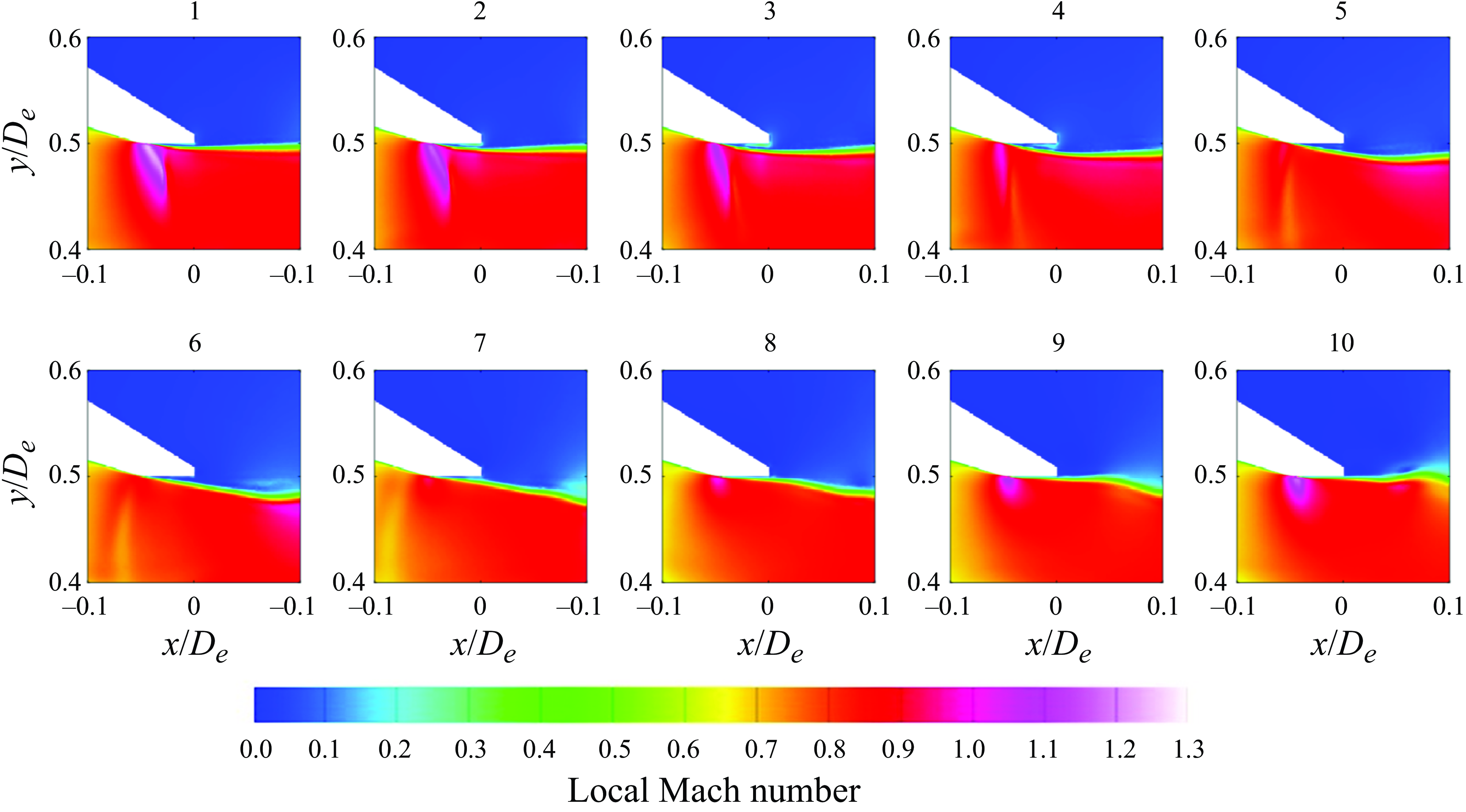
Shock-induced boundary-layer separation occurred in the vicinity of the small-radius bend in the nozzle wall and, once separation occurred, the flow was no longer required to make as sharp a turn. Supersonic flow inside the nozzle then ceased to exist and the shock vanished. The shock that induced boundary-layer separation was no longer present and the boundary layer reattached to the nozzle wall. The flow accelerated again to locally supersonic speeds in the vicinity of the small-radius, convex bend. The shock was again strong enough to separate the boundary layer, and the cycle continued periodically. In Appendix A, it is shown via experiments that the howling can be suppressed by simply adding an appropriate boundary-layer trip just upstream of the small-radius, convex bend. These results are not discussed here to avoid detracting from the study of the howling. An axial velocity spectrum was computed from the HRLES using the fluctuations at a single point along the lipline of the final nozzle and indicated that the separation occurred at a frequency of 7747.7 $\pm$
125 Hz. The frequency of oscillations found in the HRLES was greater than the typical frequency of measured flow oscillations at the same operating condition (approximately
$\pm$
125 Hz. The frequency of oscillations found in the HRLES was greater than the typical frequency of measured flow oscillations at the same operating condition (approximately $6$
kHz, as shown in § 3.1). An explanation for this is forthcoming.
$6$
kHz, as shown in § 3.1). An explanation for this is forthcoming.
A look at pressure fluctuations in the HRLES reveals that a particular acoustic mode of the nozzle’s mixing duct was energised when the SWBLI took place. A time history of pressures inside the straight cylindrical portion of the nozzle’s mixing duct at $x = -0.37D_e$
was extracted from the HRLES at a sampling rate of about 110 kHz along a radial line running from one side of the duct to the other. Considering pressures along a single line rather than the entire cross-stream plane at a given axial position was justified because the orderly oscillations in the simulation appeared axisymmetric. The pressure fluctuations were extremely orderly, as seen in the segment of the time history in figure 13(a). This shows the pressure fluctuations over 10
$x = -0.37D_e$
was extracted from the HRLES at a sampling rate of about 110 kHz along a radial line running from one side of the duct to the other. Considering pressures along a single line rather than the entire cross-stream plane at a given axial position was justified because the orderly oscillations in the simulation appeared axisymmetric. The pressure fluctuations were extremely orderly, as seen in the segment of the time history in figure 13(a). This shows the pressure fluctuations over 10 $\tau$
, where
$\tau$
, where $\tau$
is the period of the dominant oscillations. The pressure fluctuations were most powerful near the centreline of the duct. The pressure fluctuations at the duct’s wall were out of phase with and weaker than those at the duct’s centreline. Further, there was a radial position where the pressure fluctuations were nearly zero at all times: approximately a ‘pressure node.’ As will be clear shortly, this was the signature of a particular higher-order acoustic mode of the mixing duct.
$\tau$
is the period of the dominant oscillations. The pressure fluctuations were most powerful near the centreline of the duct. The pressure fluctuations at the duct’s wall were out of phase with and weaker than those at the duct’s centreline. Further, there was a radial position where the pressure fluctuations were nearly zero at all times: approximately a ‘pressure node.’ As will be clear shortly, this was the signature of a particular higher-order acoustic mode of the mixing duct.
Pressure fluctuations inside the nozzle’s mixing duct at $x=-0.37D_e=-0.39D_1$
in HRLES: (a) time history, (b) power spectral density on duct centreline and (c) radial profile of pressure-fluctuation magnitude in HRLES at
$x=-0.37D_e=-0.39D_1$
in HRLES: (a) time history, (b) power spectral density on duct centreline and (c) radial profile of pressure-fluctuation magnitude in HRLES at $f =$
7747.7
$f =$
7747.7 $\pm$
125 Hz compared with
$\pm$
125 Hz compared with $(0,1)$
acoustic mode of a round duct with uniform flow.
$(0,1)$
acoustic mode of a round duct with uniform flow. $L_e/D_e$
= 0.7,
$L_e/D_e$
= 0.7, $M_j$
= 0.90, unheated.
$M_j$
= 0.90, unheated.
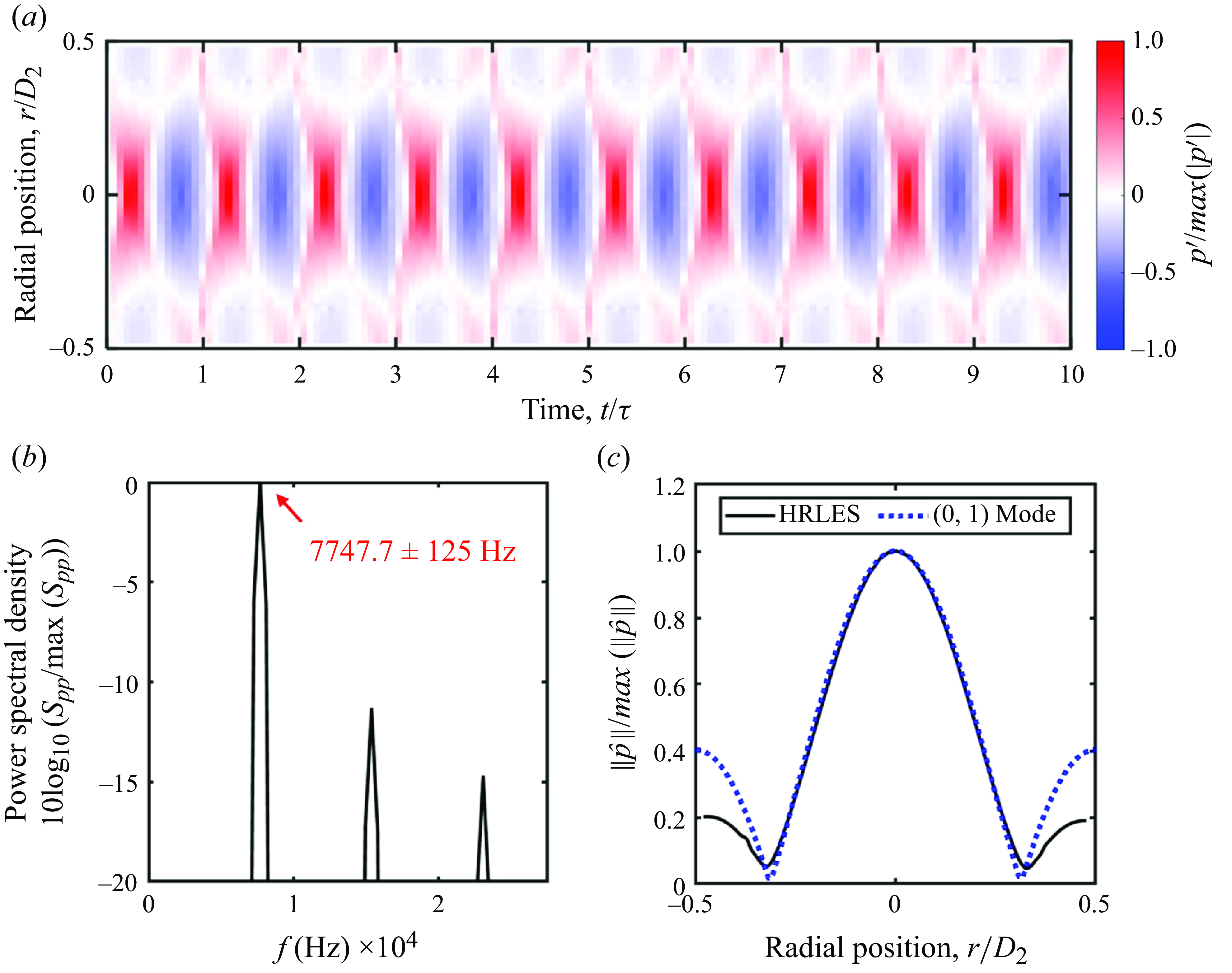
The power spectral density at the duct’s centreline estimated using single block of 440, Hanning-windowed time steps is shown in figure 13(b). A dominant 7747.7 $\pm$
125 Hz discrete frequency was present. This is the same frequency as the periodic separation in the simulation. The discrete Fourier transform (in time) of the extracted pressure fluctuations along the entire radial line was taken and the magnitude of this Fourier transform at 7747.7 Hz is shown in figure 13(c). As seen in the time history, the fluctuations are strongest near the centre of the duct at
$\pm$
125 Hz discrete frequency was present. This is the same frequency as the periodic separation in the simulation. The discrete Fourier transform (in time) of the extracted pressure fluctuations along the entire radial line was taken and the magnitude of this Fourier transform at 7747.7 Hz is shown in figure 13(c). As seen in the time history, the fluctuations are strongest near the centre of the duct at $r=0$
and exhibit an approximate pressure node between the centreline at
$r=0$
and exhibit an approximate pressure node between the centreline at $r=0$
and the mixing duct’s wall at
$r=0$
and the mixing duct’s wall at $r=D_2/2$
. Alongside the curve obtained from the HRLES, a result from classical duct acoustics is shown: the pressure-fluctuation magnitude of a round duct’s
$r=D_2/2$
. Alongside the curve obtained from the HRLES, a result from classical duct acoustics is shown: the pressure-fluctuation magnitude of a round duct’s $(0,1)$
acoustic mode in the presence of uniform flow. Aside from discrepancies at larger
$(0,1)$
acoustic mode in the presence of uniform flow. Aside from discrepancies at larger $r$
at and near the mixing-duct wall (which could be due to refraction of sound by the boundary layer near the wall), there is excellent agreement. This shows that an excitation of the mixing duct’s
$r$
at and near the mixing-duct wall (which could be due to refraction of sound by the boundary layer near the wall), there is excellent agreement. This shows that an excitation of the mixing duct’s $(0,1)$
acoustic mode accompanied the periodic SWBLI at the final nozzle’s exit. More fundamentally, this suggests that the SWBLI and associated oscillations were capable of exciting higher-order acoustic modes of the nozzle’s mixing duct. As will be evident shortly, experiments suggest that the SWBLI at the final nozzle’s exit predominantly coupled with the
$(0,1)$
acoustic mode accompanied the periodic SWBLI at the final nozzle’s exit. More fundamentally, this suggests that the SWBLI and associated oscillations were capable of exciting higher-order acoustic modes of the nozzle’s mixing duct. As will be evident shortly, experiments suggest that the SWBLI at the final nozzle’s exit predominantly coupled with the $(2,0)$
acoustic mode of the nozzle’s mixing duct at its cut-on frequency – not the
$(2,0)$
acoustic mode of the nozzle’s mixing duct at its cut-on frequency – not the $(0,1)$
mode found in the HRLES.
$(0,1)$
mode found in the HRLES.
Additional work would be required to rigorously show that the excited higher-order acoustic mode was indeed a natural acoustic mode in the simulation – although this is likely the case. As explained earlier in § 1.3, natural acoustic modes have zero axial group velocity and do not transport energy along the duct. Given the HRLES time history, showing this condition is met would require a numerical evaluation of the time-averaged acoustic energy flux through a cross-stream plane at a given axial position inside the nozzle’s mixing duct. If this time-averaged acoustic energy flux was found to be zero, then it could safely be stated that the higher-order mode excited in the simulation was a natural acoustic mode. Short of determining the group velocity, the axial phase velocity of the waves appearing in the HRLES could be compared with values for the duct’s relevant natural acoustic modes obtained by theoretical means. However, we carefully recall that, at no point during the set up of the simulations (e.g. grid refinement) were there checks that the acoustic duct modes inside the nozzle were properly resolved. Although the SWBLI consistently appeared in our simulations, the frequency of oscillation exhibited some sensitivity to the grid refinement, indicating that further computational study is required. We prefer to exercise caution and recommend that, prior to making any stronger statements regarding the HRLES and carrying out acoustic energy-flux calculations, a detailed (and computationally expensive) HRLES campaign be conducted to ensure that the acoustics of the nozzle interior are properly resolved. This substantial additional work is not pursued here, because the HRLES has served its purpose of revealing that a SWBLI was responsible for the experimentally observed periodic separation and that this SWBLI could excite the higher-order acoustic modes of the nozzle’s mixing duct.
3.4. The fundamental acoustic tone’s frequency and amplitude
Turning back to experimental data, figure 14 shows the dependence of the fundamental acoustic tone’s frequency (figure 14
a) and amplitude (figure 14
b) on $M_j$
across the range
$M_j$
across the range $0.80 \lt M_j \lt 1.00$
in steps as small as 0.01. Within this figure, data acquired using three different mixing-duct lengths (
$0.80 \lt M_j \lt 1.00$
in steps as small as 0.01. Within this figure, data acquired using three different mixing-duct lengths ( $L_e/D_e$
= 0.7, 2.0 and 3.0) are shown but measurements acquired using the
$L_e/D_e$
= 0.7, 2.0 and 3.0) are shown but measurements acquired using the $L_e/D_e$
= 0.7 mixing-duct length are discussed first.
$L_e/D_e$
= 0.7 mixing-duct length are discussed first.
In acquiring the data for the $L_e/D_e = 0.7$
mixing-duct length, acoustic measurements were made on four different days over the span of several months. On each of these days, the facility was set up as consistently as possible and measurements were made across jet Mach numbers from 0.80 to 1.00. For readability of the figure, the resulting ranges of fundamental-tone frequency and amplitude are shown (as opposed to every data point) for
$L_e/D_e = 0.7$
mixing-duct length, acoustic measurements were made on four different days over the span of several months. On each of these days, the facility was set up as consistently as possible and measurements were made across jet Mach numbers from 0.80 to 1.00. For readability of the figure, the resulting ranges of fundamental-tone frequency and amplitude are shown (as opposed to every data point) for $M_j$
at which multiple measurements were made and the fundamental tone’s frequency fit comfortably with the dominant trend in the data. Due to the onset of the howling occurring at slightly different
$M_j$
at which multiple measurements were made and the fundamental tone’s frequency fit comfortably with the dominant trend in the data. Due to the onset of the howling occurring at slightly different $M_j$
in measurements made on different days, only single data points appear at
$M_j$
in measurements made on different days, only single data points appear at $M_j = 0.81$
and
$M_j = 0.81$
and $M_j = 0.82$
. As was alluded to earlier, the howling was found to occur at
$M_j = 0.82$
. As was alluded to earlier, the howling was found to occur at $M_j$
as low as 0.81. Beginning at
$M_j$
as low as 0.81. Beginning at $M_j$
= 0.83, the
$M_j$
= 0.83, the $L_e/D_e$
= 0.7 data are shown as a narrow, shaded envelope running horizontally across the plot, indicating that the frequency of the fundamental tone was largely insensitive to
$L_e/D_e$
= 0.7 data are shown as a narrow, shaded envelope running horizontally across the plot, indicating that the frequency of the fundamental tone was largely insensitive to $M_j$
. For
$M_j$
. For $0.94 \leq M_j \leq 0.97$
, however, there are three data markers that appear above this envelope, indicating that the fundamental tone sometimes occurred at a higher frequency. All three of these higher-frequency data markers correspond to measurements made on the same day, and it is not presently clear what caused this. Only speculation is possible, which we avoid here.
$0.94 \leq M_j \leq 0.97$
, however, there are three data markers that appear above this envelope, indicating that the fundamental tone sometimes occurred at a higher frequency. All three of these higher-frequency data markers correspond to measurements made on the same day, and it is not presently clear what caused this. Only speculation is possible, which we avoid here.
The frequency of periodic separation in the HRLES simulations (7747.7 $\pm$
125 Hz) was somewhat close to the frequency of these higher-frequency data markers, as shown by the data at
$\pm$
125 Hz) was somewhat close to the frequency of these higher-frequency data markers, as shown by the data at $M_j = 0.90$
labelled ‘HRLES simulation (
$M_j = 0.90$
labelled ‘HRLES simulation ( $L_e/D_e$
= 0.7).’ As
$L_e/D_e$
= 0.7).’ As $M_j$
approached unity, the howling ceased. Measurements were made at
$M_j$
approached unity, the howling ceased. Measurements were made at $M_j$
= 0.99 on some days, but no tones were visible in spectra measured at this operating condition. The curves which run nearly horizontally across the plot show the cut-on frequencies of the mixing duct’s higher-order acoustic modes that fell close to the measured frequencies. These cut-on frequencies will be discussed shortly.
$M_j$
= 0.99 on some days, but no tones were visible in spectra measured at this operating condition. The curves which run nearly horizontally across the plot show the cut-on frequencies of the mixing duct’s higher-order acoustic modes that fell close to the measured frequencies. These cut-on frequencies will be discussed shortly.
In figure 14(b), the grey, shaded envelope shows that there was substantial scatter in the fundamental tone’s amplitude on the different occasions it was measured, despite care taken to ensure the experimental set-up was as consistent as possible. Due to this scatter, not much may be said about the fundamental tone’s amplitude. It does appear, however, that the highest-amplitude tones were measured at $0.86 \leq M_j \leq 0.88$
. The scatter is particularly large at
$0.86 \leq M_j \leq 0.88$
. The scatter is particularly large at $M_j = 0.90$
. Further statements about this variation in tone amplitude would require an additional experimental campaign of many repeated experiments. Because we do not study the tone’s amplitude in great detail here, these additional experiments are not pursued. However, we can say that this day-to-day variation was larger than experiments repeated in close succession on the same day. A relatively small difference of
$M_j = 0.90$
. Further statements about this variation in tone amplitude would require an additional experimental campaign of many repeated experiments. Because we do not study the tone’s amplitude in great detail here, these additional experiments are not pursued. However, we can say that this day-to-day variation was larger than experiments repeated in close succession on the same day. A relatively small difference of $2$
dB has been observed between running the jet at
$2$
dB has been observed between running the jet at $M_j = 0.90$
, then an operating condition that did not produce any howling and then
$M_j = 0.90$
, then an operating condition that did not produce any howling and then $M_j= 0.90$
again without shutting off the flow. We focus on the tone’s frequency in pursuit of an understanding of the observed howling.
$M_j= 0.90$
again without shutting off the flow. We focus on the tone’s frequency in pursuit of an understanding of the observed howling.
Measured fundamental acoustic tone with unheated core-stream (a) frequency and (b) sound pressure level (SPL) for several $M_j$
for three different mixing-duct lengths. (
$M_j$
for three different mixing-duct lengths. ( $\theta$
= 90
$\theta$
= 90 $^{\circ }$
, lossless, fully corrected, projected to
$^{\circ }$
, lossless, fully corrected, projected to $R$
= 84.7
$R$
= 84.7 $D_e$
, and
$D_e$
, and $\Delta f$
= 2.5 Hz.)
$\Delta f$
= 2.5 Hz.)
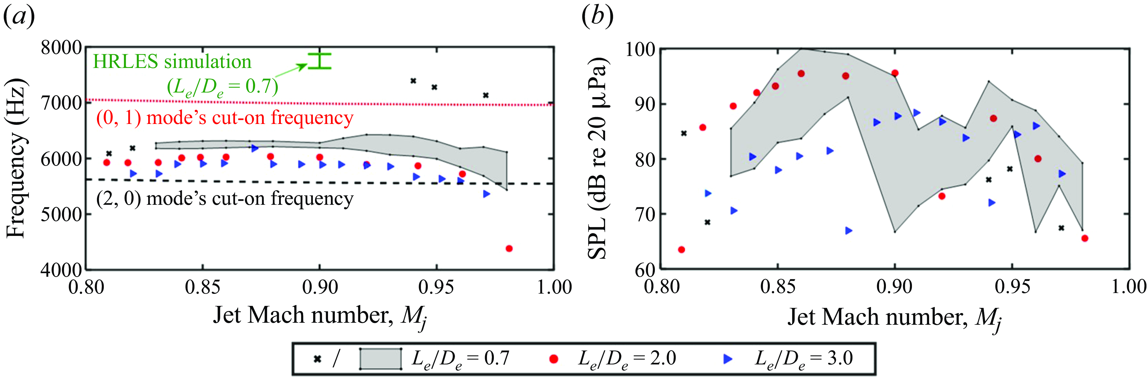
Returning to figure 14(a), increasing the nozzle’s mixing-duct length reduced the fundamental tone’s frequency slightly, and an explanation for this will be put forth in § 4. It is noted with caution (due to the large scatter in the fundamental tone’s amplitude mentioned in the previous paragraph) that the longer mixing-duct lengths tended to produce lower-amplitude fundamental tones, as seen in figure 14(b). Of course, this was not always the case. For example, at $M_j$
= 0.91 the
$M_j$
= 0.91 the $L_e/D_e$
= 3.0 mixing-duct length produced a tone that was of higher amplitude than the
$L_e/D_e$
= 3.0 mixing-duct length produced a tone that was of higher amplitude than the $L_e/D_e$
= 0.7 mixing-duct length produced during any of the many measurements made. With the measurements corresponding to the two longer mixing-duct lengths made on only one occasion, it is reasonable to expect that, had the measurements been repeated several times, the longer mixing-duct lengths would have produced a scatter in the fundamental tone’s amplitude similar to what is shown by the grey, shaded envelope corresponding to the
$L_e/D_e$
= 0.7 mixing-duct length produced during any of the many measurements made. With the measurements corresponding to the two longer mixing-duct lengths made on only one occasion, it is reasonable to expect that, had the measurements been repeated several times, the longer mixing-duct lengths would have produced a scatter in the fundamental tone’s amplitude similar to what is shown by the grey, shaded envelope corresponding to the $L_e/D_e$
= 0.7 mixing-duct length. Therefore, not much may be said about the role of the mixing-duct length on the fundamental tone’s amplitude.
$L_e/D_e$
= 0.7 mixing-duct length. Therefore, not much may be said about the role of the mixing-duct length on the fundamental tone’s amplitude.
In figure 14(a), the curves show the cut-on frequencies of the nozzle’s round mixing duct that were nearest the measured tone frequencies: those of the $(2,0)$
and
$(2,0)$
and $(0,1)$
modes. The procedure used to calculate these cut-on frequencies is outlined in Appendix B. There are no cut-on frequencies that lie between those of the
$(0,1)$
modes. The procedure used to calculate these cut-on frequencies is outlined in Appendix B. There are no cut-on frequencies that lie between those of the $(2,0)$
and
$(2,0)$
and $(0,1)$
modes, and the cut-on frequencies were nearly constant across the range of
$(0,1)$
modes, and the cut-on frequencies were nearly constant across the range of $M_j$
plotted. This is because, although the cut-on frequencies do depend on
$M_j$
plotted. This is because, although the cut-on frequencies do depend on $M_j$
, as
$M_j$
, as $M_j$
increases from 0.80 to 1.00, the Mach number of the flow inside the mixing duct only increases slightly from 0.433 to 0.454 (according to quasi-one-dimensional, isentropic-flow calculations). As explained earlier in § 1.3, the cut-on frequencies are natural frequencies of the mixing duct at which aeroacoustic feedback phenomena are particularly likely to occur, provided a suitable, sound-generating flow instability exists at a nearby frequency. In the present case, this flow instability is the SWBLI near the final-nozzle exit – although the specific sound-generation mechanisms are not studied in detail in this paper. There is good agreement between the calculated cut-on frequencies and the measured tone frequencies, suggesting that the natural acoustic modes of the nozzle’s round mixing duct indeed coupled with the SWBLI in a feedback phenomenon that led to the observed howling. A coupling to the
$M_j$
increases from 0.80 to 1.00, the Mach number of the flow inside the mixing duct only increases slightly from 0.433 to 0.454 (according to quasi-one-dimensional, isentropic-flow calculations). As explained earlier in § 1.3, the cut-on frequencies are natural frequencies of the mixing duct at which aeroacoustic feedback phenomena are particularly likely to occur, provided a suitable, sound-generating flow instability exists at a nearby frequency. In the present case, this flow instability is the SWBLI near the final-nozzle exit – although the specific sound-generation mechanisms are not studied in detail in this paper. There is good agreement between the calculated cut-on frequencies and the measured tone frequencies, suggesting that the natural acoustic modes of the nozzle’s round mixing duct indeed coupled with the SWBLI in a feedback phenomenon that led to the observed howling. A coupling to the $(2,0)$
natural acoustic mode appears to predominate coupling with the
$(2,0)$
natural acoustic mode appears to predominate coupling with the $(0,1)$
natural acoustic mode at a slightly higher frequency. This may occur because the cut-on frequency of the
$(0,1)$
natural acoustic mode at a slightly higher frequency. This may occur because the cut-on frequency of the $(2,0)$
mode was closer to the characteristic frequency of the SWBLI (i.e. the frequency it would tend to occur at in the absence of acoustic coupling). A substantial research effort would be required to rigorously support this, as the characteristic frequency of the SWBLI is not presently known.
$(2,0)$
mode was closer to the characteristic frequency of the SWBLI (i.e. the frequency it would tend to occur at in the absence of acoustic coupling). A substantial research effort would be required to rigorously support this, as the characteristic frequency of the SWBLI is not presently known.
The reader may recall that the signature of the mixing duct’s $(0,1)$
acoustic mode was found in the HRLES. A detailed HRLES simulation campaign would be required to explain this discrepancy, and this is beyond the scope of this paper. However, we again emphasise that the HRLES has served its purpose of showing that the SWBLI was the root cause for the periodic separation observed in the experiments and that the SWBLI can excite a higher-order acoustic mode of the nozzle’s mixing duct. In what follows, we focus on the
$(0,1)$
acoustic mode was found in the HRLES. A detailed HRLES simulation campaign would be required to explain this discrepancy, and this is beyond the scope of this paper. However, we again emphasise that the HRLES has served its purpose of showing that the SWBLI was the root cause for the periodic separation observed in the experiments and that the SWBLI can excite a higher-order acoustic mode of the nozzle’s mixing duct. In what follows, we focus on the $(2,0)$
acoustic mode because its cut-on frequency was in close agreement with the majority of the measured fundamental-tone frequencies in experimental data in figure 14(a). Although the measured frequencies were consistently higher than the calculated cut-on frequencies, an explanation for this is put forth in § 4.
$(2,0)$
acoustic mode because its cut-on frequency was in close agreement with the majority of the measured fundamental-tone frequencies in experimental data in figure 14(a). Although the measured frequencies were consistently higher than the calculated cut-on frequencies, an explanation for this is put forth in § 4.
We briefly note that natural acoustic modes of longitudinal nature (i.e. involving waves travelling along the axis of the mixing duct) cannot explain the measured trends because the fundamental tone’s frequency was relatively insensitive to $L_e$
.
$L_e$
.
3.5. Azimuthal order of the oscillations
As shown in § 3.1, the fundamental tones are attended by a periodic boundary-layer separation at the final-nozzle exit and an excitation of instability waves in the final jet at the same frequency. In § 3.3, we showed that this separation was caused by a periodic SWBLI inside the nozzle which excited an acoustic mode of the nozzle’s mixing duct. Basic calculations provided in § 3.4 indicated that the predominantly observed howling frequency was close to the cut-on frequency of an acoustic mode of the nozzle’s mixing duct. These observations alone strongly suggest that the howling was the result of a feedback phenomenon between the SWBLI and a natural acoustic mode of the nozzle’s mixing duct. Again, this coupling seems to predominantly involve the $(2,0)$
acoustic mode of the nozzle’s mixing duct. Before proceeding to more-sophisticated models for estimating the cut-on frequencies of the mixing duct’s higher-order acoustic modes, additional experimental data are provided. These data further support that a coupling between the SWBLI and the mixing duct’s
$(2,0)$
acoustic mode of the nozzle’s mixing duct. Before proceeding to more-sophisticated models for estimating the cut-on frequencies of the mixing duct’s higher-order acoustic modes, additional experimental data are provided. These data further support that a coupling between the SWBLI and the mixing duct’s $(2,0)$
acoustic mode took place when the howling occurred.
$(2,0)$
acoustic mode took place when the howling occurred.
The feedback phenomenon studied here was, as explained several times now, caused by a coupling between the SWBLI and a natural acoustic mode of the nozzle’s mixing duct. In the event of such a coupling, the SWBLI that excited the natural acoustic mode will also be influenced by the natural acoustic mode. Both should exhibit the same azimuthal order. The instability waves excited in the final jet as a result of this coupling should exhibit this same azimuthal order, too. Measurements and accompanying theory appearing in § 4.5 of Ramsey (Reference Ramsey2024) provide extensive evidence that this is the case. For completeness, a select few velocity-field measurements obtained via stereoscopic PIV appearing in that reference are presented here. A description of the measurement system is foregone here but may be found in § 4.5 of (Ramsey Reference Ramsey2024), along with careful checks of the accuracy of the measured data.
Figure 15 shows a baseline PIV dataset obtained using the $L_e/D_e = 0.7$
configuration of the nozzle at an operating condition that did not produce any howling:
$L_e/D_e = 0.7$
configuration of the nozzle at an operating condition that did not produce any howling: $M_j = 0.70$
, unheated flow. These data were obtained in a cross-stream plane at
$M_j = 0.70$
, unheated flow. These data were obtained in a cross-stream plane at $x = 2D_e$
downstream of the final nozzle’s exit. The reader should imagine the jet axis pointed out of the page when inspecting these data. Figure 15(a) shows the axial mean velocity,
$x = 2D_e$
downstream of the final nozzle’s exit. The reader should imagine the jet axis pointed out of the page when inspecting these data. Figure 15(a) shows the axial mean velocity, $U$
. This measured mean velocity was normalised by the ideally expanded core-jet velocity (
$U$
. This measured mean velocity was normalised by the ideally expanded core-jet velocity ( $U_{j1}$
), which was nominally the same as that of the bypass stream at this operating condition. Figure 15(b) shows the axial turbulence intensity, which was computed as the standard deviation of axial velocity fluctuations (
$U_{j1}$
), which was nominally the same as that of the bypass stream at this operating condition. Figure 15(b) shows the axial turbulence intensity, which was computed as the standard deviation of axial velocity fluctuations ( $\sigma _x$
) normalised by the ideally expanded core-jet velocity. These data were obtained from an ensemble of
$\sigma _x$
) normalised by the ideally expanded core-jet velocity. These data were obtained from an ensemble of $N$
= 750 independent snapshots of the velocity field, which yielded suitable convergence of the mean and standard deviation of the velocity. Both the mean velocity and turbulence intensities seen are typical of a turbulent, round jet and compare well with the well-accepted published data (e.g. see Ahuja et al. (Reference Ahuja, Lepicovsky and Burrin1982); Bridges & Wernet (Reference Bridges and Wernet2011)).
$N$
= 750 independent snapshots of the velocity field, which yielded suitable convergence of the mean and standard deviation of the velocity. Both the mean velocity and turbulence intensities seen are typical of a turbulent, round jet and compare well with the well-accepted published data (e.g. see Ahuja et al. (Reference Ahuja, Lepicovsky and Burrin1982); Bridges & Wernet (Reference Bridges and Wernet2011)).
Velocity-field measurements in a cross-stream plane at $x/D_e$
= 2 with
$x/D_e$
= 2 with $M_j=0.70$
, unheated: (a) axial mean and (b) axial turbulence intensity.
$M_j=0.70$
, unheated: (a) axial mean and (b) axial turbulence intensity. $N = 750$
snapshots averaged.
$N = 750$
snapshots averaged. $L_e/D_e = 0.7$
.
$L_e/D_e = 0.7$
.
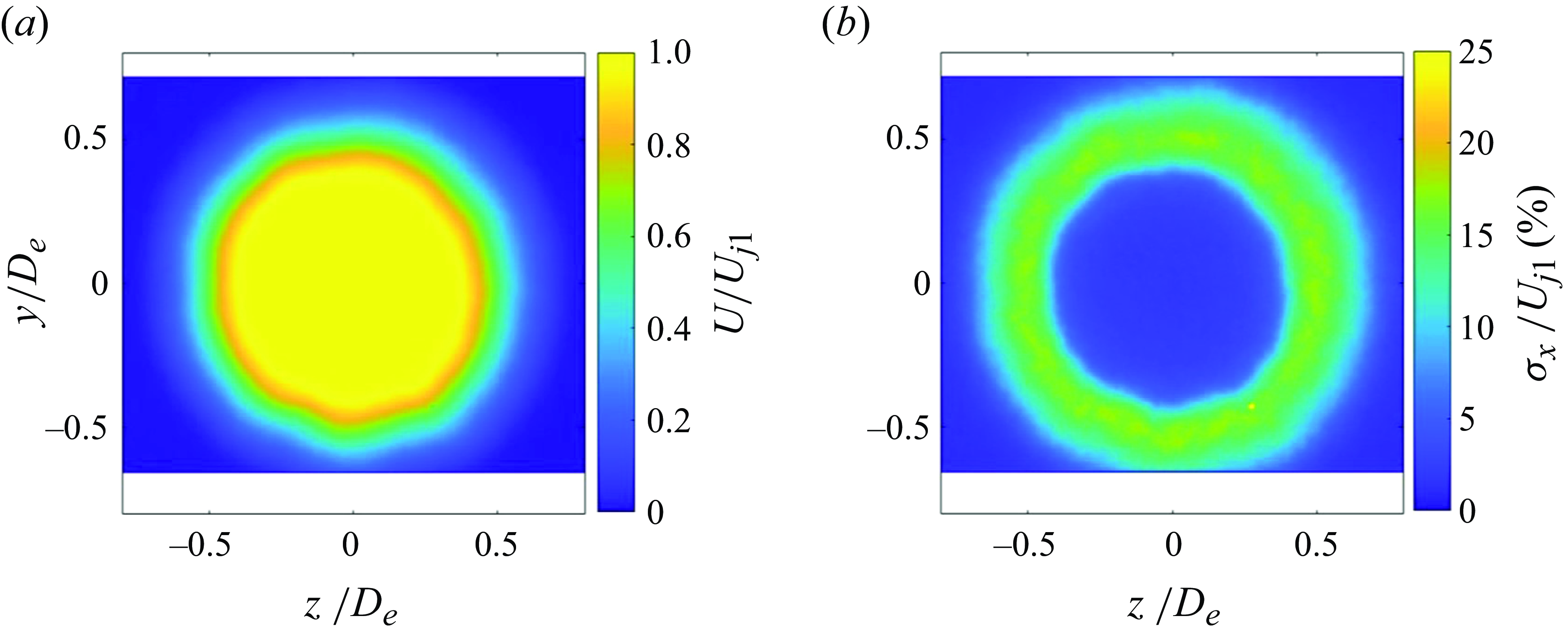
Velocity-field measurements in a cross-stream plane at $x/D_e$
= 2 with
$x/D_e$
= 2 with $M_j = 0.90$
, unheated: (a) axial mean and (b) axial turbulence intensity.
$M_j = 0.90$
, unheated: (a) axial mean and (b) axial turbulence intensity. $N = 750$
snapshots averaged.
$N = 750$
snapshots averaged. $L_e/D_e = 0.7$
.
$L_e/D_e = 0.7$
.
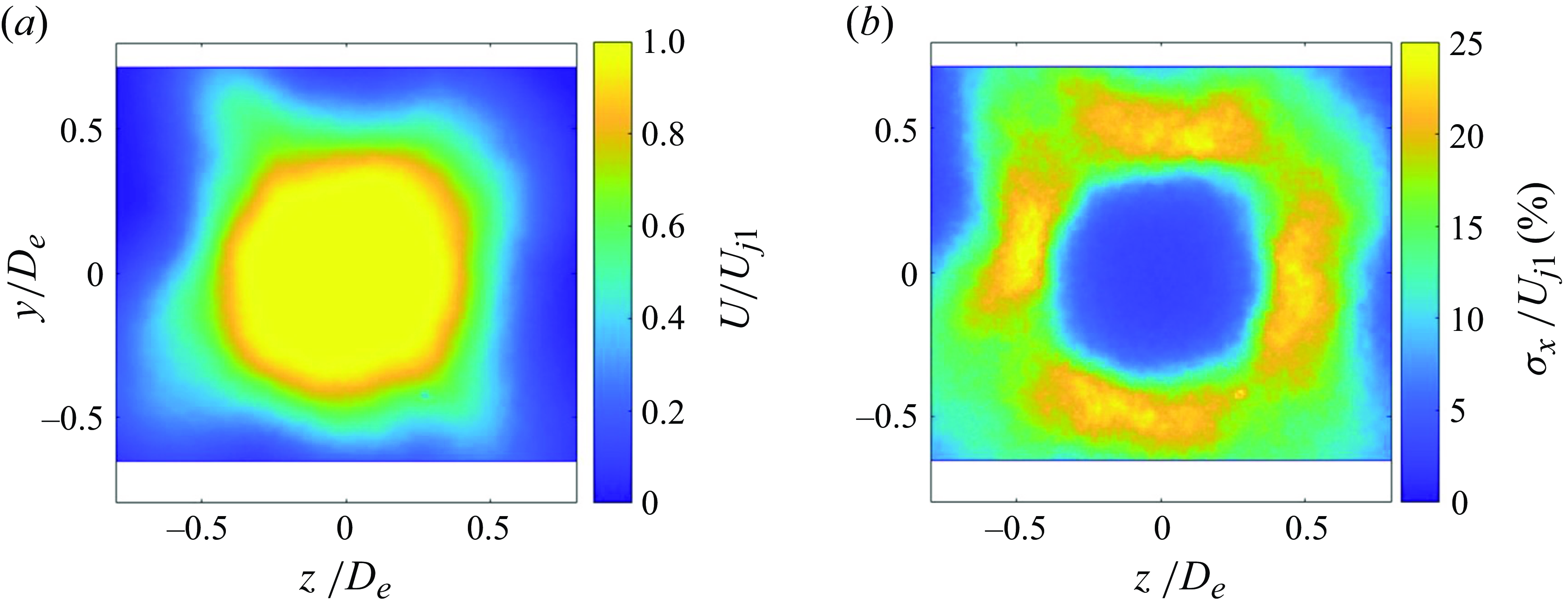
Velocity-field measurements in a cross-stream plane at $x/D_e$
= 1 with
$x/D_e$
= 1 with $M_j = 0.90$
, unheated: (a) axial mean and (b) axial turbulence intensity.
$M_j = 0.90$
, unheated: (a) axial mean and (b) axial turbulence intensity. $N = 750$
snapshots averaged.
$N = 750$
snapshots averaged. $L_e/D_e = 0.7$
.
$L_e/D_e = 0.7$
.
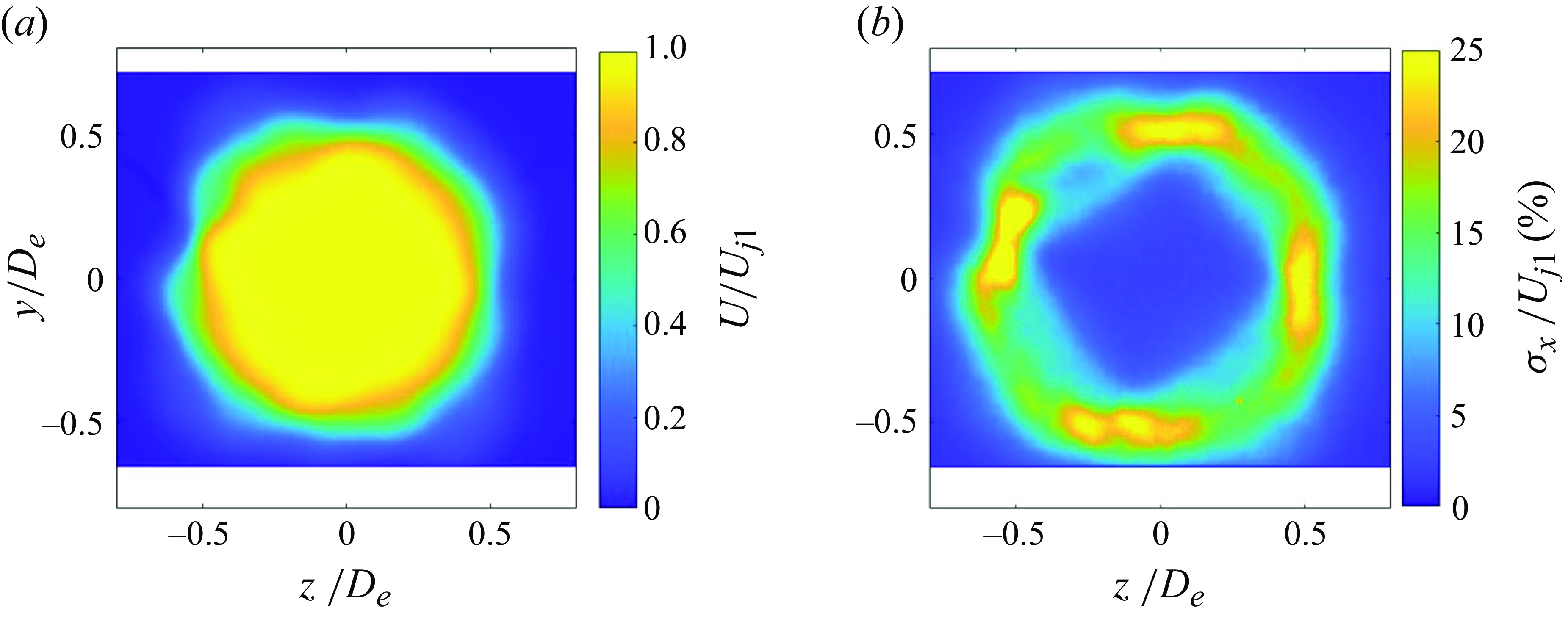
Figure 16 shows measurements made using the same nozzle configuration at an operating condition that produced the howling: $M_j = 0.90$
, unheated flow. Figure 16(a) reveals a distorted mean flow, and figure 16(b) shows that the axial turbulence intensity is higher in the presence of the howling. This is expected of an excited jet. What is not expected is that there are four localised regions of relatively high turbulence intensity in the jet’s shear layer at 90-degree intervals from one another. This pattern is yet clearer in data obtained closer to the final-nozzle exit at
$M_j = 0.90$
, unheated flow. Figure 16(a) reveals a distorted mean flow, and figure 16(b) shows that the axial turbulence intensity is higher in the presence of the howling. This is expected of an excited jet. What is not expected is that there are four localised regions of relatively high turbulence intensity in the jet’s shear layer at 90-degree intervals from one another. This pattern is yet clearer in data obtained closer to the final-nozzle exit at $x = D_e$
in figure 17. If the instability waves excited in the final jet were axisymmetric (
$x = D_e$
in figure 17. If the instability waves excited in the final jet were axisymmetric ( $m=0$
), the turbulence intensity would also appear nominally axisymmetric. Had these instability waves been flapping (one variety of
$m=0$
), the turbulence intensity would also appear nominally axisymmetric. Had these instability waves been flapping (one variety of $m=1$
instability waves that do not spin about the jet axis), there would be two regions of locally high turbulence intensity appearing on opposing sides of the jet. Although perhaps not obvious at first, these patterns in the measured turbulence intensity are the signature of
$m=1$
instability waves that do not spin about the jet axis), there would be two regions of locally high turbulence intensity appearing on opposing sides of the jet. Although perhaps not obvious at first, these patterns in the measured turbulence intensity are the signature of $m = 2$
instability waves that remain preferentially oriented, rather than spinning about the jet axis. These waves might be suitably called ‘pinching’ instability waves due to their appearance in a cross-stream plane. These experimental data thus support that the feedback phenomenon involved a coupling between the SWBLI and the
$m = 2$
instability waves that remain preferentially oriented, rather than spinning about the jet axis. These waves might be suitably called ‘pinching’ instability waves due to their appearance in a cross-stream plane. These experimental data thus support that the feedback phenomenon involved a coupling between the SWBLI and the $(2,0)$
acoustic mode of the nozzle’s mixing duct. This is shown more rigorously in § 4.5 of Ramsey (Reference Ramsey2024) through comparisons with results of linear stability theory, where it is also shown that the same patterns discussed here can be found in measured PIV data obtained on five different days over the span of one month without modifying the experimental set-up. Other data appearing in that reference indicate the excited instability waves have
$(2,0)$
acoustic mode of the nozzle’s mixing duct. This is shown more rigorously in § 4.5 of Ramsey (Reference Ramsey2024) through comparisons with results of linear stability theory, where it is also shown that the same patterns discussed here can be found in measured PIV data obtained on five different days over the span of one month without modifying the experimental set-up. Other data appearing in that reference indicate the excited instability waves have $m = 2$
azimuthal order, too.
$m = 2$
azimuthal order, too.
4. Natural frequencies of mixing duct with non-uniform flow
Now, with evidence that the SWBLI predominantly coupled to the $(2,0)$
acoustic mode of the nozzle’s mixing duct, we use more-sophisticated models to improve estimates of this mode’s cut-on frequency and extend these estimates to heated core operating conditions.
$(2,0)$
acoustic mode of the nozzle’s mixing duct, we use more-sophisticated models to improve estimates of this mode’s cut-on frequency and extend these estimates to heated core operating conditions.
4.1. Further experimental data
The frequency of the fundamental tone was shown to be largely insensitive to $M_j$
and
$M_j$
and $L_e$
above in figure 14. However, the fundamental tone’s frequency was sensitive to
$L_e$
above in figure 14. However, the fundamental tone’s frequency was sensitive to $T_{t1}$
, as shown here in figure 18, where the total temperatures reported are averages across entire microphone recording durations. Figures 18(a) and 18(b) correspond to two different tests conducted using the
$T_{t1}$
, as shown here in figure 18, where the total temperatures reported are averages across entire microphone recording durations. Figures 18(a) and 18(b) correspond to two different tests conducted using the $L_e/D_e = 0.7$
mixing-duct length, which are denoted ‘test 1’ and ‘test 2’. The ‘test 1’ data shown in figure 18(a) were measured as follows. The nozzle was operated at
$L_e/D_e = 0.7$
mixing-duct length, which are denoted ‘test 1’ and ‘test 2’. The ‘test 1’ data shown in figure 18(a) were measured as follows. The nozzle was operated at $M_j$
= 0.90, and then the core stream’s burner was lit. Subsequently,
$M_j$
= 0.90, and then the core stream’s burner was lit. Subsequently, $T_{t1}$
rose to about 600 K (
$T_{t1}$
rose to about 600 K ( $TTR_1 \approx 2$
) over approximately 30 minutes. A total of 45 typical, 45-second microphone recordings were acquired during this period. For approximately 30 minutes,
$TTR_1 \approx 2$
) over approximately 30 minutes. A total of 45 typical, 45-second microphone recordings were acquired during this period. For approximately 30 minutes, $T_{t1}$
was held around 600 K and a total of 15 45-second microphone recordings were acquired. Then, the burner was shut off and the jet was continuously run while the facility cooled. During this cooling period, a total of 34 shorter, 20-second microphone recordings were acquired with hopes of capturing the temperature dependence with a finer resolution in time. The ‘test 2’ data shown in figure 18(b) were measured on a different day, and a similar procedure was conducted with 20-second recordings acquired throughout. During test 2,
$T_{t1}$
was held around 600 K and a total of 15 45-second microphone recordings were acquired. Then, the burner was shut off and the jet was continuously run while the facility cooled. During this cooling period, a total of 34 shorter, 20-second microphone recordings were acquired with hopes of capturing the temperature dependence with a finer resolution in time. The ‘test 2’ data shown in figure 18(b) were measured on a different day, and a similar procedure was conducted with 20-second recordings acquired throughout. During test 2, $T_{t1}$
was only allowed to rise to about 525 K (
$T_{t1}$
was only allowed to rise to about 525 K ( $TTR_1 \approx$
1.77) and 31 recordings were obtained during this time. The burner was shut off immediately at that temperature (a practical decision made to reduce the test’s duration), and another 23 recordings were obtained as the temperature decreased.
$TTR_1 \approx$
1.77) and 31 recordings were obtained during this time. The burner was shut off immediately at that temperature (a practical decision made to reduce the test’s duration), and another 23 recordings were obtained as the temperature decreased.
Measured fundamental acoustic tone’s frequency as a function of core-stream total temperature ( $L_e/D_e = 0.7$
): (a) test 1 and (b) test 2. (
$L_e/D_e = 0.7$
): (a) test 1 and (b) test 2. ( $\theta$
= 90
$\theta$
= 90 $^{\circ }$
,
$^{\circ }$
, $\Delta f$
= 2.5 Hz.)
$\Delta f$
= 2.5 Hz.)
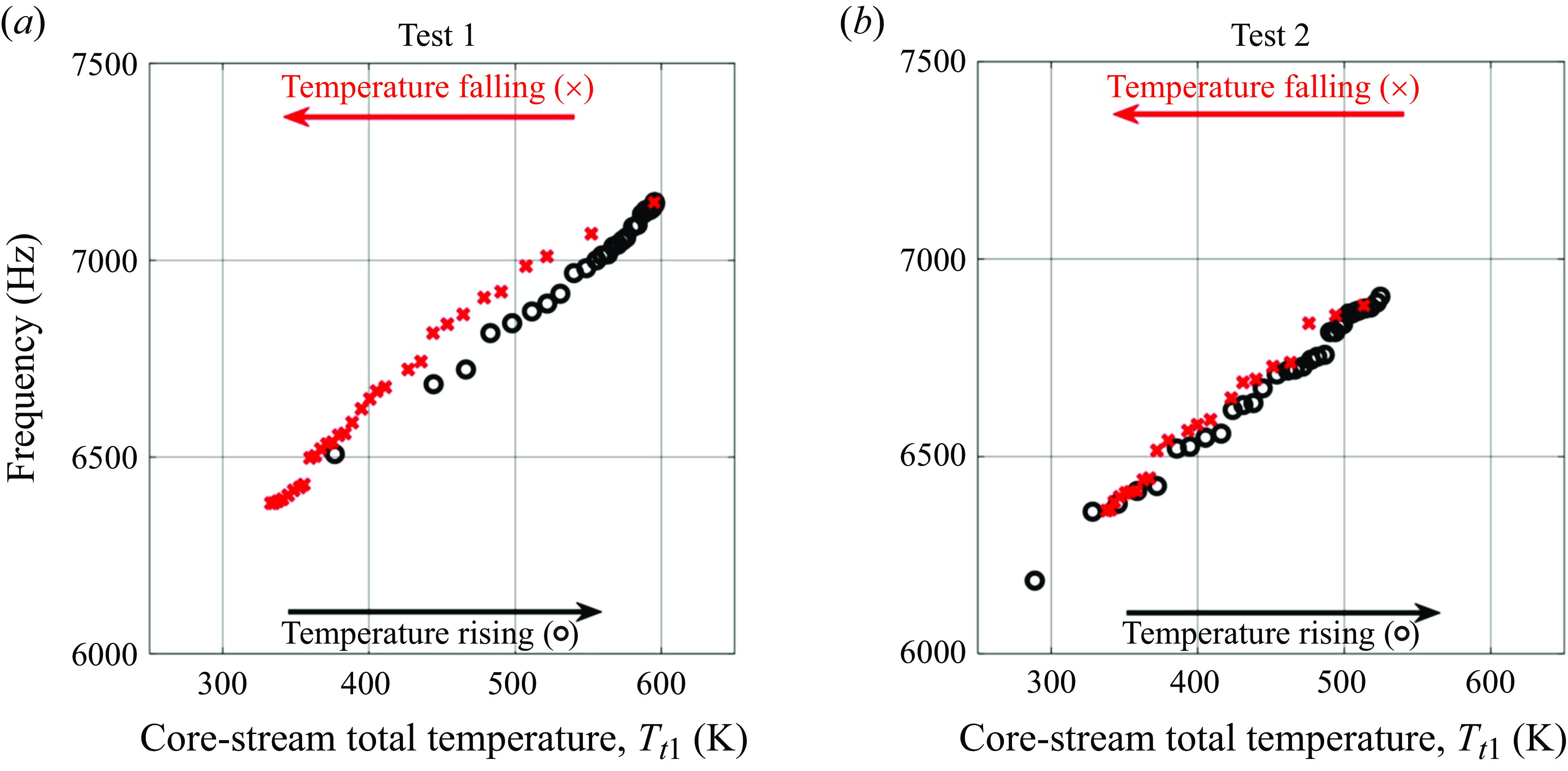
By comparing the test 1 data in figure 18(a) and test 2 data in figure 18(b), it can be seen that the fundamental tone’s frequency had a repeatable dependence on $T_{t1}$
. This will be made clearer in the following figures that show both datasets on the same plot (e.g. figure 20). The frequency of the fundamental tone increased with
$T_{t1}$
. This will be made clearer in the following figures that show both datasets on the same plot (e.g. figure 20). The frequency of the fundamental tone increased with $T_{t1}$
, varying more than 500 Hz as
$T_{t1}$
, varying more than 500 Hz as $T_{t1}$
increased from 300 to 600 K. A minor difference between temperature-rising and temperature-falling measurements may be seen in the test 1 data in figure 18(a) around
$T_{t1}$
increased from 300 to 600 K. A minor difference between temperature-rising and temperature-falling measurements may be seen in the test 1 data in figure 18(a) around $T_{t1} \approx 500$
K, with temperature-rising and temperature-falling measurements differing by approximately 100 Hz. This is believed to be due to residual heat given off by the nozzle hardware during the temperature-falling measurements. Due to the relatively long duration of test 1, the core nozzle was likely heat soaked before the temperature-falling measurements began. Due to the heat given off by the heat-soaked core nozzle, some of the air flowing through the nozzle was likely at a higher temperature when it reached the mixing duct than the upstream total temperature measurements suggested, resulting in a higher-frequency fundamental tone.
$T_{t1} \approx 500$
K, with temperature-rising and temperature-falling measurements differing by approximately 100 Hz. This is believed to be due to residual heat given off by the nozzle hardware during the temperature-falling measurements. Due to the relatively long duration of test 1, the core nozzle was likely heat soaked before the temperature-falling measurements began. Due to the heat given off by the heat-soaked core nozzle, some of the air flowing through the nozzle was likely at a higher temperature when it reached the mixing duct than the upstream total temperature measurements suggested, resulting in a higher-frequency fundamental tone.
If the cut-on frequency of the mixing duct’s $(2,0)$
acoustic mode truly set the frequency of the fundamental acoustic tone, then calculations of the cut-on frequency corresponding to heated core operating conditions should reveal the same trend as shown in figure 18. With the core stream heated, the core and bypass streams have different temperatures and velocities in the mixing duct and a uniform-flow assumption cannot be made to calculate cut-on frequencies as was done in the previous section.
$(2,0)$
acoustic mode truly set the frequency of the fundamental acoustic tone, then calculations of the cut-on frequency corresponding to heated core operating conditions should reveal the same trend as shown in figure 18. With the core stream heated, the core and bypass streams have different temperatures and velocities in the mixing duct and a uniform-flow assumption cannot be made to calculate cut-on frequencies as was done in the previous section.
4.2. A dual-stream vortex-sheet model
An inviscid vortex-sheet model illustrated in figure 19 approximates the mean flow in the mixing duct as two, uniform-velocity regions separated by an infinitely thin shear layer located at $r = R_1$
(
$r = R_1$
( $r$
is the radial coordinate), which was selected to be the inner radius of the core nozzle (
$r$
is the radial coordinate), which was selected to be the inner radius of the core nozzle ( $R_1 = 20.3$
mm). This dual-stream flow is confined within a round, rigid duct with radius
$R_1 = 20.3$
mm). This dual-stream flow is confined within a round, rigid duct with radius $R_2$
which was set to the radius of the mixing duct (
$R_2$
which was set to the radius of the mixing duct ( $R_2= 26.3$
mm). The details of this model problem are not new, and have been used in the past by Ahuja et al. (Reference Ahuja, Massey, Fleming, Tam and III1992) and Viswanathan, Morris & Chen (Reference Viswanathan, Morris and Chen1994) to analyse ducted supersonic jets, for example. The dispersion relation for this model problem is given in Appendix C for completeness.
$R_2= 26.3$
mm). The details of this model problem are not new, and have been used in the past by Ahuja et al. (Reference Ahuja, Massey, Fleming, Tam and III1992) and Viswanathan, Morris & Chen (Reference Viswanathan, Morris and Chen1994) to analyse ducted supersonic jets, for example. The dispersion relation for this model problem is given in Appendix C for completeness.
Dual-stream vortex-sheet model: (a) axial view and (b) cross-sectional view.
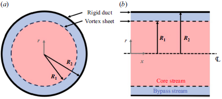
With the model problem selected, the flow properties for each stream remain to be prescribed. The Mach number inside the nozzle’s mixing duct was calculated using isentropic and quasi-one-dimensional compressible-flow equations. With $M_j = 0.90$
and the area consumed by the core-nozzle lip subtracted from the area of the mixing duct, the mixing-duct Mach number was found to be
$M_j = 0.90$
and the area consumed by the core-nozzle lip subtracted from the area of the mixing duct, the mixing-duct Mach number was found to be $M = 0.449$
. The total pressure and the specific heats of both streams are the same such that, even in the heated core operating conditions, a quasi-one-dimensional analysis suggests that the two streams have the same
$M = 0.449$
. The total pressure and the specific heats of both streams are the same such that, even in the heated core operating conditions, a quasi-one-dimensional analysis suggests that the two streams have the same $M$
inside the mixing duct. With the stagnation temperatures and pressures prescribed, all needed flow properties were known.
$M$
inside the mixing duct. With the stagnation temperatures and pressures prescribed, all needed flow properties were known.
For a given set of flow conditions, the cut-on frequency of the mixing duct’s $(2,0)$
acoustic mode was then obtained by searching for neutral-wave solutions of the dispersion relation (i.e. frequency and wavenumber were real-valued) using a zero-searching algorithm implemented in MATLAB. The calculated cut-on frequency of the mixing duct’s
$(2,0)$
acoustic mode was then obtained by searching for neutral-wave solutions of the dispersion relation (i.e. frequency and wavenumber were real-valued) using a zero-searching algorithm implemented in MATLAB. The calculated cut-on frequency of the mixing duct’s $(2,0)$
acoustic mode is shown in figure 20 as a function of
$(2,0)$
acoustic mode is shown in figure 20 as a function of $T_{t1}$
along with all measured data from figure 18. The increase in frequency with increasing
$T_{t1}$
along with all measured data from figure 18. The increase in frequency with increasing $T_{t1}$
seen in the measurements is captured well by the calculations, inspiring even greater confidence in our understanding of the mechanism responsible for the howling. However, a minor discrepancy remains. The calculated
$T_{t1}$
seen in the measurements is captured well by the calculations, inspiring even greater confidence in our understanding of the mechanism responsible for the howling. However, a minor discrepancy remains. The calculated $(2,0)$
mode’s cut-on frequency is consistently lower than the measured tone frequencies. This discrepancy was also seen in the comparisons of calculated cut-on frequencies and measured tone frequencies at unheated operating conditions shown earlier in figure 14. We propose that the
$(2,0)$
mode’s cut-on frequency is consistently lower than the measured tone frequencies. This discrepancy was also seen in the comparisons of calculated cut-on frequencies and measured tone frequencies at unheated operating conditions shown earlier in figure 14. We propose that the $(2,0)$
mode’s cut-on frequencies have consistently fallen below the measured tone frequencies due to neglecting the wake of the core nozzle in the model. In what follows, this wake is accounted for.
$(2,0)$
mode’s cut-on frequencies have consistently fallen below the measured tone frequencies due to neglecting the wake of the core nozzle in the model. In what follows, this wake is accounted for.
Cut-on frequency of $(2,0)$
acoustic mode of mixing duct calculated using dual-stream vortex-sheet model (
$(2,0)$
acoustic mode of mixing duct calculated using dual-stream vortex-sheet model ( $M = 0.449$
,
$M = 0.449$
, $T_{t2}$
= 293 K) compared with measured data from figure 18 (data from test 1 and test 2 both plotted). (Measurements made at
$T_{t2}$
= 293 K) compared with measured data from figure 18 (data from test 1 and test 2 both plotted). (Measurements made at $\theta$
= 90
$\theta$
= 90 $^{\circ }$
with
$^{\circ }$
with $\Delta f$
= 2.5 Hz.)
$\Delta f$
= 2.5 Hz.)
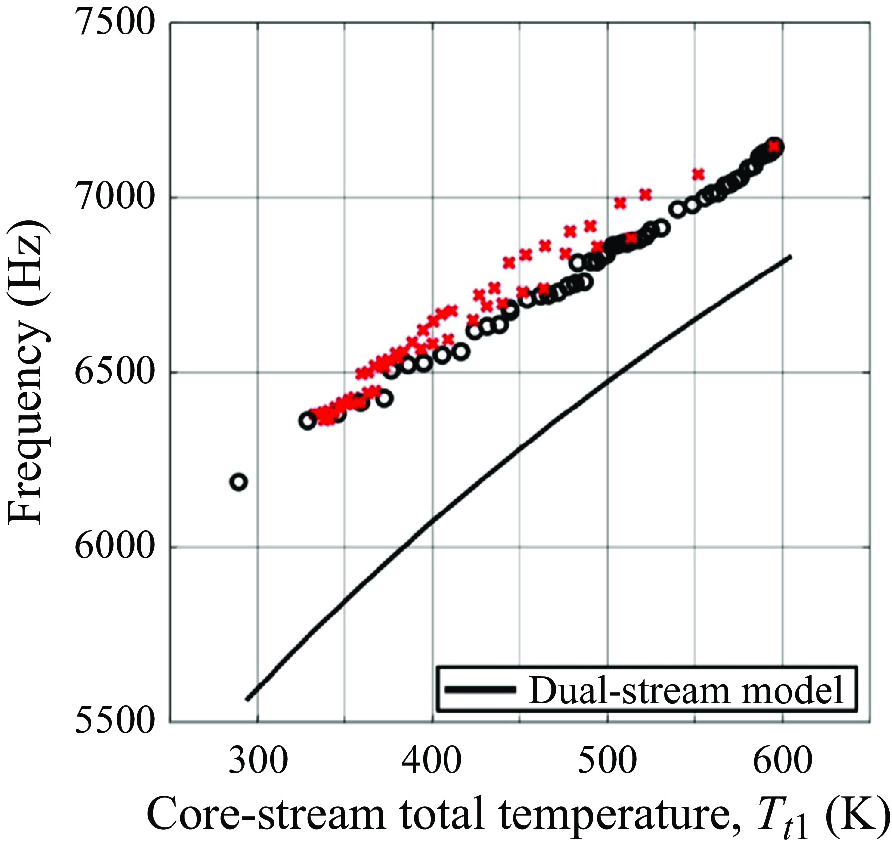
4.3. Accounting for the core nozzle’s wake
To account for the core-nozzle wake, a different vortex-sheet model was used: a ‘tri-stream vortex-sheet model’ as illustrated in figure 21. In this model, a third, annular stream was included between the core and bypass streams to model the wake of the core nozzle. The velocity in the wake region was set to zero unless otherwise noted, and the static temperature of the wake was taken to be equal to $(T_{1}+T_{2})/2$
, where
$(T_{1}+T_{2})/2$
, where $T_1$
and
$T_1$
and $T_2$
are the static temperatures of the core and bypass stream inside the mixing duct (in absolute units) calculated using isentropic-flow equations. This latter assumption is justified by noting that the wake will be heated to some degree when the core stream was heated due to the simple fact that the core-nozzle hardware itself was at an elevated temperature. The static pressure inside the mixing duct was found as a function of the mixing-duct Mach number
$T_2$
are the static temperatures of the core and bypass stream inside the mixing duct (in absolute units) calculated using isentropic-flow equations. This latter assumption is justified by noting that the wake will be heated to some degree when the core stream was heated due to the simple fact that the core-nozzle hardware itself was at an elevated temperature. The static pressure inside the mixing duct was found as a function of the mixing-duct Mach number $M$
and the stagnation pressure, and the fluid properties of the wake were then known. The wake region’s inner radius
$M$
and the stagnation pressure, and the fluid properties of the wake were then known. The wake region’s inner radius $R_1$
and outer radius
$R_1$
and outer radius $R_\alpha$
were not constrained to match the core nozzle’s inner and outer radii. Due to the presence of boundary layers on the inner and outer surfaces of the core nozzle and the possibility of instabilities in the wake (e.g. vortex shedding from the core-nozzle lip), we allowed for the wake region to be thicker than the core-nozzle lip itself. The value of
$R_\alpha$
were not constrained to match the core nozzle’s inner and outer radii. Due to the presence of boundary layers on the inner and outer surfaces of the core nozzle and the possibility of instabilities in the wake (e.g. vortex shedding from the core-nozzle lip), we allowed for the wake region to be thicker than the core-nozzle lip itself. The value of $M$
used for the tri-stream vortex-sheet model was taken to be that used in the dual-stream vortex-sheet model. This is left unjustified for now, but will be revisited at the end of this section.
$M$
used for the tri-stream vortex-sheet model was taken to be that used in the dual-stream vortex-sheet model. This is left unjustified for now, but will be revisited at the end of this section.
Tri-stream vortex-sheet model: (a) axial view and (b) cross-sectional view.
To convey the wake dimensions in a concise manner, additional notation was needed. The thickness of the wake is defined as $\delta \equiv R_{\alpha } - R_{1}$
and alternatively expressed as
$\delta \equiv R_{\alpha } - R_{1}$
and alternatively expressed as $\delta = \delta _0 + \delta _- + \delta _+$
, where
$\delta = \delta _0 + \delta _- + \delta _+$
, where $\delta _0$
is the true thickness of the core-nozzle lip and
$\delta _0$
is the true thickness of the core-nozzle lip and $\delta _-$
and
$\delta _-$
and $\delta _+$
are the thicknesses of the wake region on the inside and outside of the core-nozzle lip, respectively. A so-called ‘wake-skew ratio’ defined as
$\delta _+$
are the thicknesses of the wake region on the inside and outside of the core-nozzle lip, respectively. A so-called ‘wake-skew ratio’ defined as $\beta \equiv \delta _-/\delta _+$
is used to indicate a radial offset of the wake’s centre from the true centre of the core-nozzle lip. For example, if
$\beta \equiv \delta _-/\delta _+$
is used to indicate a radial offset of the wake’s centre from the true centre of the core-nozzle lip. For example, if $\beta \gt 1$
, the wake was centred at a smaller radius than the centre of the core-nozzle lip. If
$\beta \gt 1$
, the wake was centred at a smaller radius than the centre of the core-nozzle lip. If $\beta = 1$
, the centre of the wake was aligned with the centre of the core-nozzle lip. In figures reporting calculations made using the tri-stream vortex-sheet model, the extent of the wake region will be shown graphically to eliminate any possible confusion. The dispersion relation for the tri-stream vortex-sheet model was derived as part of the present work and is given in Appendix D in its general form (i.e. the velocity in the wake region was not assumed zero for the derivation). As done for the dual-stream vortex-sheet model, the cut-on frequencies were found as neutral-wave solutions of the dispersion relation (i.e. frequency and wavenumber were real valued) using a zero-searching algorithm implemented in MATLAB.
$\beta = 1$
, the centre of the wake was aligned with the centre of the core-nozzle lip. In figures reporting calculations made using the tri-stream vortex-sheet model, the extent of the wake region will be shown graphically to eliminate any possible confusion. The dispersion relation for the tri-stream vortex-sheet model was derived as part of the present work and is given in Appendix D in its general form (i.e. the velocity in the wake region was not assumed zero for the derivation). As done for the dual-stream vortex-sheet model, the cut-on frequencies were found as neutral-wave solutions of the dispersion relation (i.e. frequency and wavenumber were real valued) using a zero-searching algorithm implemented in MATLAB.
The sensitivity of tri-stream vortex-sheet model calculations of the $(2,0)$
mode’s cut-on frequency to
$(2,0)$
mode’s cut-on frequency to $\delta$
with
$\delta$
with $\beta = 4$
is shown in figure 22. The diagram in figure 22(a) illustrates the radial extent of the wake for three different wake thicknesses. In figure 22(b), increased
$\beta = 4$
is shown in figure 22. The diagram in figure 22(a) illustrates the radial extent of the wake for three different wake thicknesses. In figure 22(b), increased $\delta$
(with
$\delta$
(with $\beta = 4$
) is shown to increase the
$\beta = 4$
) is shown to increase the $(2,0)$
mode’s cut-on frequency in a uniform manner across the entire range of
$(2,0)$
mode’s cut-on frequency in a uniform manner across the entire range of $T_{t1}$
plotted. The sensitivity of the calculations to
$T_{t1}$
plotted. The sensitivity of the calculations to $\beta$
(with
$\beta$
(with $\delta / \delta _0 = 8$
) is shown in figure 23. The diagram in figure 23(a) illustrates the extent of the wake region for four different values of
$\delta / \delta _0 = 8$
) is shown in figure 23. The diagram in figure 23(a) illustrates the extent of the wake region for four different values of $\beta$
. Figure 23(b) shows that increased
$\beta$
. Figure 23(b) shows that increased $\beta$
decreases the
$\beta$
decreases the $(2,0)$
mode’s cut-on frequency, with
$(2,0)$
mode’s cut-on frequency, with $\beta$
having no influence when
$\beta$
having no influence when $T_{t1} = T_{t2}$
and having an increasingly strong effect as
$T_{t1} = T_{t2}$
and having an increasingly strong effect as $T_{t1}$
is increased above
$T_{t1}$
is increased above $T_{t2}$
. This may be understood as follows.
$T_{t2}$
. This may be understood as follows.
For a given $\delta$
, increasing
$\delta$
, increasing $\beta$
shifts the wake radially inward. This shift of the wake results in a smaller cross-sectional area being consumed by the core stream and wake, and the cross-sectional area consumed by the bypass stream is increased. With a heated core stream, this reduces the cross-sectional area consumed by the hotter core stream and wake, and increases the cross-sectional area consumed by the cooler bypass stream. This change can be shown to decrease the
$\beta$
shifts the wake radially inward. This shift of the wake results in a smaller cross-sectional area being consumed by the core stream and wake, and the cross-sectional area consumed by the bypass stream is increased. With a heated core stream, this reduces the cross-sectional area consumed by the hotter core stream and wake, and increases the cross-sectional area consumed by the cooler bypass stream. This change can be shown to decrease the $(2,0)$
mode’s cut-on frequency even with zero mean flow, and thus the sensitivity to
$(2,0)$
mode’s cut-on frequency even with zero mean flow, and thus the sensitivity to $\beta$
is the result of a modified sound-speed distribution inside the duct.
$\beta$
is the result of a modified sound-speed distribution inside the duct.
Effect of wake thickness for a given wake-skew ratio ( $\beta = 4$
): (a) illustration of wake’s radial extent relative to core nozzle and mixing-duct wall and (b)
$\beta = 4$
): (a) illustration of wake’s radial extent relative to core nozzle and mixing-duct wall and (b) $(2,0)$
mode’s cut-on frequency as a function of
$(2,0)$
mode’s cut-on frequency as a function of $T_{t1}$
. (
$T_{t1}$
. ( $M = 0.449$
,
$M = 0.449$
, $T_{t2}$
= 293 K.)
$T_{t2}$
= 293 K.)

Effect of different wake-skew ratios, $\beta$
, with
$\beta$
, with $\delta /\delta _0 = 8$
: (a) illustration of wake’s radial extent relative to core nozzle and mixing-duct wall and (b)
$\delta /\delta _0 = 8$
: (a) illustration of wake’s radial extent relative to core nozzle and mixing-duct wall and (b) $(2,0)$
mode’s cut-on frequency as a function of
$(2,0)$
mode’s cut-on frequency as a function of $T_{t1}$
. (
$T_{t1}$
. ( $M = 0.449$
,
$M = 0.449$
, $T_{t2}$
= 293 K.)
$T_{t2}$
= 293 K.)
By taking $\delta /\delta _0 = 8$
and
$\delta /\delta _0 = 8$
and $\beta = 4$
, the calculated
$\beta = 4$
, the calculated $(2,0)$
mode’s cut-on frequency was in excellent agreement with the measured tone’s frequency, as shown in figure 24. It is noted that the calculated cut-on frequency still fell below the measured frequency at lower
$(2,0)$
mode’s cut-on frequency was in excellent agreement with the measured tone’s frequency, as shown in figure 24. It is noted that the calculated cut-on frequency still fell below the measured frequency at lower $T_{t1}$
, but making the already-thick wake any thicker to improve the agreement seemed physically unjustifiable. We also avoided further complicating the model (e.g. by making
$T_{t1}$
, but making the already-thick wake any thicker to improve the agreement seemed physically unjustifiable. We also avoided further complicating the model (e.g. by making $\delta$
and
$\delta$
and $\beta$
dependent upon
$\beta$
dependent upon $T_{t1}$
) to improve this discrepancy.
$T_{t1}$
) to improve this discrepancy.
Cut-on frequency of $(2,0)$
acoustic mode of mixing duct calculated using both vortex-sheet models (
$(2,0)$
acoustic mode of mixing duct calculated using both vortex-sheet models ( $M = 0.449, T_{t2} = 293$
K) compared with data from figure 18 (data from test 1 and test 2 both plotted). (Acoustic measurements made at
$M = 0.449, T_{t2} = 293$
K) compared with data from figure 18 (data from test 1 and test 2 both plotted). (Acoustic measurements made at $\theta$
= 90
$\theta$
= 90 $^{\circ }$
and have
$^{\circ }$
and have $\Delta f$
= 2.5 Hz.)
$\Delta f$
= 2.5 Hz.)
The curious reader may wonder how the pressure profiles of the $(2,0)$
acoustic modes (i.e. the pressure eigenfunctions) compare with those of classical acoustic duct modes in the presence of uniform flow. Only minor changes are observed at the cut-on frequencies, as shown via example pressure eigenfunctions shown in Appendix E.
$(2,0)$
acoustic modes (i.e. the pressure eigenfunctions) compare with those of classical acoustic duct modes in the presence of uniform flow. Only minor changes are observed at the cut-on frequencies, as shown via example pressure eigenfunctions shown in Appendix E.
4.4. Comparing the modelled and computed wake
Admittedly, $\delta$
and
$\delta$
and $\beta$
were tuned until the calculations matched well with the experimental data, rendering the calculations an empirical fit of sorts. The thorough reader may be critical of this, and may wonder how the geometry of the modelled wake and true wake compare. We provide a comparison in figure 25 between the mean flow obtained via HRLES and the radial extent of the modelled wake for the inviscid vortex-sheet model. Figure 25(a) shows the local-Mach-number distribution throughout the nozzle at the
$\beta$
were tuned until the calculations matched well with the experimental data, rendering the calculations an empirical fit of sorts. The thorough reader may be critical of this, and may wonder how the geometry of the modelled wake and true wake compare. We provide a comparison in figure 25 between the mean flow obtained via HRLES and the radial extent of the modelled wake for the inviscid vortex-sheet model. Figure 25(a) shows the local-Mach-number distribution throughout the nozzle at the $M_j = 0.90$
, unheated operating condition. The white space corresponds to the solid cross-sectional area of the nozzle, and the colour indicates the computed local Mach number. The darker colour appearing downstream of the core-nozzle lip (see
$M_j = 0.90$
, unheated operating condition. The white space corresponds to the solid cross-sectional area of the nozzle, and the colour indicates the computed local Mach number. The darker colour appearing downstream of the core-nozzle lip (see $r/D_1\approx 0.5$
,
$r/D_1\approx 0.5$
, $x/D_1\approx -0.7$
) indicates the location of the most severe velocity deficit due to the wake of the core nozzle. Notably, the centre of the wake is directed slightly radially inward inside the nozzle’s mixing duct. The two solid black lines indicate the radial extent of the wake assumed in the inviscid vortex-sheet model with
$x/D_1\approx -0.7$
) indicates the location of the most severe velocity deficit due to the wake of the core nozzle. Notably, the centre of the wake is directed slightly radially inward inside the nozzle’s mixing duct. The two solid black lines indicate the radial extent of the wake assumed in the inviscid vortex-sheet model with $\delta /\delta _0=8$
and
$\delta /\delta _0=8$
and $\beta = 4$
. A more quantitative comparison is offered in figure 25(b), where radial profiles of the mean local Mach number are compared with the inviscid profile that agreed best with the measured data. The wake assumed for the inviscid flow model is unsurprisingly thicker than the wake visible in the HRLES mean Mach-number profile; however, the computed wake is nearly centred in the wake assumed for the inviscid profile. We believe that, although thicker than the computed wake visible in the mean Mach-number profiles, the assumed wake for the inviscid flow model is reasonable.
$\beta = 4$
. A more quantitative comparison is offered in figure 25(b), where radial profiles of the mean local Mach number are compared with the inviscid profile that agreed best with the measured data. The wake assumed for the inviscid flow model is unsurprisingly thicker than the wake visible in the HRLES mean Mach-number profile; however, the computed wake is nearly centred in the wake assumed for the inviscid profile. We believe that, although thicker than the computed wake visible in the mean Mach-number profiles, the assumed wake for the inviscid flow model is reasonable.
Local Mach number inside nozzle obtained from HRLES and extent of wake assumed for inviscid flow model with $\delta /\delta _0 = 8$
and
$\delta /\delta _0 = 8$
and $\beta = 4$
: (a) local Mach-number distribution and (b) radial profiles at three axial positions. Here,
$\beta = 4$
: (a) local Mach-number distribution and (b) radial profiles at three axial positions. Here, $L_e/D_e = 0.7$
,
$L_e/D_e = 0.7$
, $M_j = 0.90$
, unheated.
$M_j = 0.90$
, unheated.
No assertion is made that the modelled wake should have the exact same geometry (thickness, say) as the true wake. After all, the simplicity of the vortex-sheet model used (e.g. the mean-velocity profile is assumed to be piecewise uniform) means that the wake used in the model should be thought of as an effective wake at best. For example, the boundary layer along the mixing duct’s wall, following Mason (Reference Mason1969) and Swinbanks (Reference Swinbanks1975), could slightly increase the cut-on frequencies of the duct. This offers one additional, possible reason why the calculated cut-on frequencies tended to be lower than the measured frequencies. Accounting for two realistic flow features (the core-nozzle wake and the boundary layer along the mixing-duct wall) would require yet more sophisticated modelling and is not pursued here. Further, the minor non-uniformity seen in the computed mean flow outside the wake is not accounted for. Cut-on frequency estimates that use the computed mean flow directly are also possible, but require more-complicated techniques not pursued here. Short of further research, the inviscid flow model used to capture the wake provides a reasonable explanation for why the calculated cut-on frequencies tended to be lower than the measured frequencies.
4.5. Mixing-length dependence of the howling frequency
As a final comparison of vortex-sheet model calculations and measurements, we briefly consider the measured dependence of the fundamental tone’s frequency on the mixing-duct length when the core stream was unheated (shown in figure 14
a). These data showed that increasing the mixing-duct length from $L_e/D_e$
= 0.7 to 3.0 reduced the fundamental tone’s frequency from between 6200 and 6300 Hz to approximately 5900 Hz. A similar mixing-duct-length dependence was also seen in the measurements published by Ramsey et al. (Reference Ramsey, Mayo, Karon, Funk and Ahuja2022b
), where increasing
$L_e/D_e$
= 0.7 to 3.0 reduced the fundamental tone’s frequency from between 6200 and 6300 Hz to approximately 5900 Hz. A similar mixing-duct-length dependence was also seen in the measurements published by Ramsey et al. (Reference Ramsey, Mayo, Karon, Funk and Ahuja2022b
), where increasing $L_e/D_e$
from 0.7 to 3.0 reduced the fundamental tone’s frequency from approximately 6100 to approximately 5700 Hz. Overall, experiments have suggested that increasing the mixing-duct length may reduce the fundamental tone’s frequency by between 300 and 400 Hz.
$L_e/D_e$
from 0.7 to 3.0 reduced the fundamental tone’s frequency from approximately 6100 to approximately 5700 Hz. Overall, experiments have suggested that increasing the mixing-duct length may reduce the fundamental tone’s frequency by between 300 and 400 Hz.
One might consider the boundary layer along the mixing duct’s wall as a possible explanation for the reduction in the howling frequency as the mixing duct was made longer. As the mixing duct’s length is increased, the maximum thickness of the boundary layer along the mixing duct’s wall will be greater. Thus, again following Mason (Reference Mason1969) and Swinbanks (Reference Swinbanks1975), a thickening of the boundary layer associated with increasing the mixing duct’s length would tend to increase the cut-on frequencies of the duct’s higher-order acoustic modes. This is opposite the measured trend.
Considering the wake of the core-nozzle lip offers a suitable explanation for this measured trend. As the mixing-duct length of the nozzle is increased, it is expected that the core nozzle’s wake is weaker (the wake has a reduced velocity deficit, say) when it reaches the downstream end of the mixing duct near where the periodic SWBLI occurred. A wake-strength parameter is used in what follows, and is defined as $\sigma \equiv 1 - U_w/U$
, where
$\sigma \equiv 1 - U_w/U$
, where $U_w$
is the mean velocity in the wake and
$U_w$
is the mean velocity in the wake and $U$
is the mean velocity of both the core and bypass streams used in the tri-stream vortex-sheet model (these are equal because only cases with unheated flow are considered in what follows). As a reminder, the wake velocity was set to zero in all preceding analyses. Examples of three mean-velocity profiles with three different
$U$
is the mean velocity of both the core and bypass streams used in the tri-stream vortex-sheet model (these are equal because only cases with unheated flow are considered in what follows). As a reminder, the wake velocity was set to zero in all preceding analyses. Examples of three mean-velocity profiles with three different $\sigma$
(
$\sigma$
( $\delta /\delta _0 = 8$
,
$\delta /\delta _0 = 8$
, $\beta = 4$
) are shown in figure 26(a) for clarity. Figure 26(b) shows that, as the wake strength was decreased from 1 to 0, the cut-on frequency of the
$\beta = 4$
) are shown in figure 26(a) for clarity. Figure 26(b) shows that, as the wake strength was decreased from 1 to 0, the cut-on frequency of the $(2,0)$
mode of the mixing duct decreased by about 350 Hz – commensurate with the frequency reduction observed experimentally when
$(2,0)$
mode of the mixing duct decreased by about 350 Hz – commensurate with the frequency reduction observed experimentally when $L_e/D_e$
was increased from 0.7 to 3.0. Therefore, it seems that the dependence of the fundamental tone’s frequency on the mixing-duct length could have been due to the wake of the core nozzle becoming weaker (at the downstream end of the mixing duct, where the SWBLI occurred) as the mixing-duct length was increased.
$L_e/D_e$
was increased from 0.7 to 3.0. Therefore, it seems that the dependence of the fundamental tone’s frequency on the mixing-duct length could have been due to the wake of the core nozzle becoming weaker (at the downstream end of the mixing duct, where the SWBLI occurred) as the mixing-duct length was increased.
Effect of wake strength on cut-on frequency of $(2,0)$
acoustic mode of mixing duct with core stream unheated: (a) example mean-velocity profiles for three different wake strengths and (b) calculated cut-on frequency as a function of wake strength. (
$(2,0)$
acoustic mode of mixing duct with core stream unheated: (a) example mean-velocity profiles for three different wake strengths and (b) calculated cut-on frequency as a function of wake strength. ( $M = 0.449, T_{t1} = T_{t2} = 293$
K,
$M = 0.449, T_{t1} = T_{t2} = 293$
K, $\beta = 4$
, and
$\beta = 4$
, and $\delta /\delta _0 = 8$
.)
$\delta /\delta _0 = 8$
.)
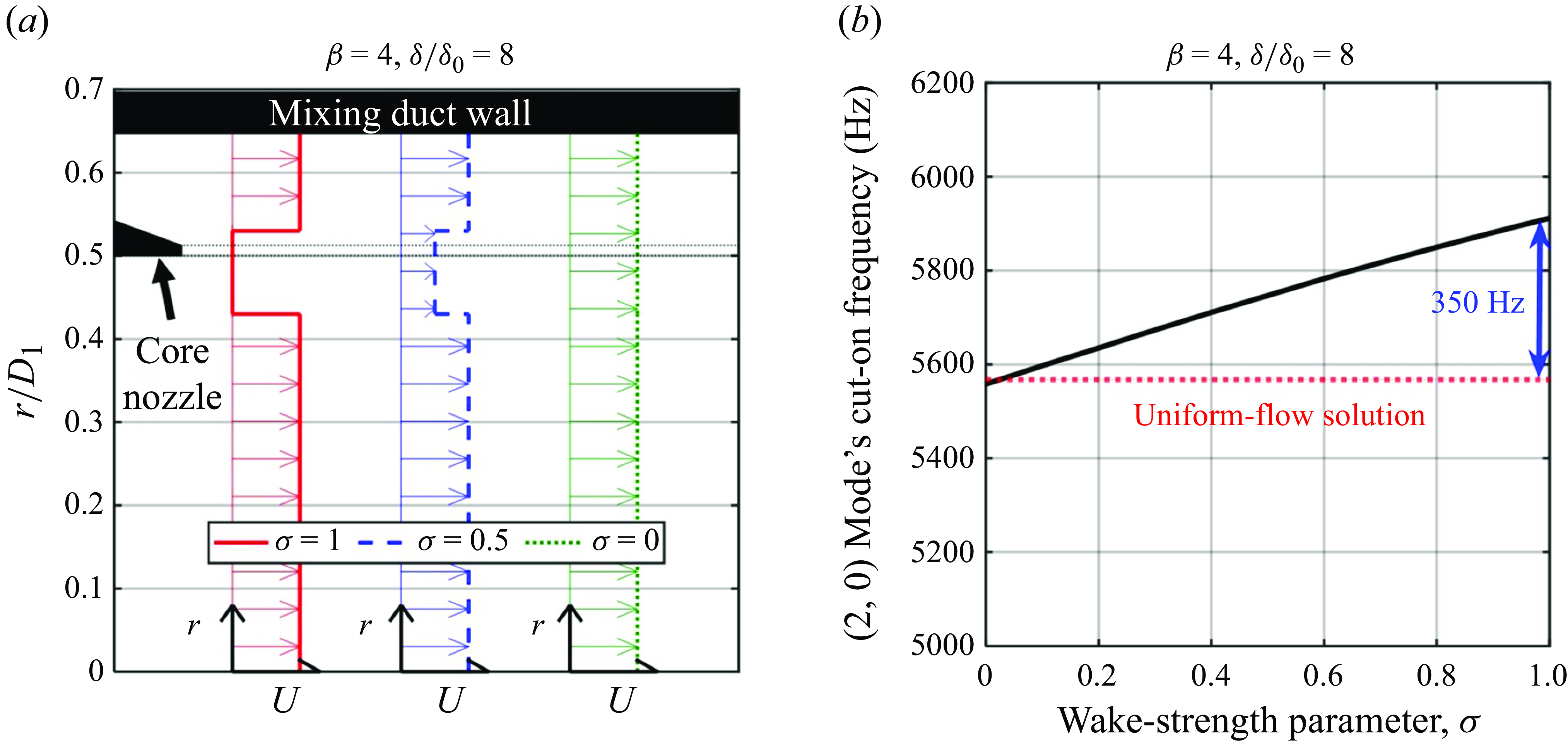
4.6. Sensitivity of vortex-sheet model results to Mach number
As noted earlier, the mixing-duct Mach number $M$
used in the tri-stream vortex-sheet model calculations was simply taken to be equal to that used in the dual-stream vortex-sheet model calculations. This assumption reduced undue complexity in our analysis, although
$M$
used in the tri-stream vortex-sheet model calculations was simply taken to be equal to that used in the dual-stream vortex-sheet model calculations. This assumption reduced undue complexity in our analysis, although $M$
might be expected to vary depending on the characteristics of the wake prescribed inside the mixing duct. For example, introducing a zero-velocity wake downstream of the core-nozzle lip reduces the effective flow area inside the mixing duct. Depending on the extent of the wake at the final-nozzle exit, the presence of this wake may change
$M$
might be expected to vary depending on the characteristics of the wake prescribed inside the mixing duct. For example, introducing a zero-velocity wake downstream of the core-nozzle lip reduces the effective flow area inside the mixing duct. Depending on the extent of the wake at the final-nozzle exit, the presence of this wake may change $M$
. In what follows, we avoid these complications and simply show that the tri-stream vortex-sheet model calculations are insensitive to changes (
$M$
. In what follows, we avoid these complications and simply show that the tri-stream vortex-sheet model calculations are insensitive to changes ( $\pm$
5 %) in
$\pm$
5 %) in $M$
.
$M$
.
Figure 27(a) shows that the calculations made using the dual-stream model change in a minor but appreciable way with $M$
– but, in this case, the procedure used to calculate
$M$
– but, in this case, the procedure used to calculate $M$
was sound. More importantly, the tri-stream model calculations (using
$M$
was sound. More importantly, the tri-stream model calculations (using $\delta /\delta _0 = 8$
,
$\delta /\delta _0 = 8$
, $\beta = 4$
) are extremely insensitive to the Mach number used as shown on the right in figure 27(b). This indicates that, while
$\beta = 4$
) are extremely insensitive to the Mach number used as shown on the right in figure 27(b). This indicates that, while $M$
could be made to depend on
$M$
could be made to depend on $\beta$
,
$\beta$
, $\delta$
and
$\delta$
and $L_e$
, complicating the analysis in this way is not likely to yield much improvement. Even if the value of
$L_e$
, complicating the analysis in this way is not likely to yield much improvement. Even if the value of $M$
used for the analysis was not exactly correct, inserting a zero-velocity annulus between the core and bypass streams as a model for the wake of the core nozzle increased the calculated cut-on frequencies – providing reasonable explanations for why the cut-on frequencies of the dual-stream model fell below the measured ones and why increasing the nozzle’s mixing-duct length decreased the fundamental tone’s frequency.
$M$
used for the analysis was not exactly correct, inserting a zero-velocity annulus between the core and bypass streams as a model for the wake of the core nozzle increased the calculated cut-on frequencies – providing reasonable explanations for why the cut-on frequencies of the dual-stream model fell below the measured ones and why increasing the nozzle’s mixing-duct length decreased the fundamental tone’s frequency.
Sensitivity of cut-on frequency calculations to mixing-duct Mach number $M$
: (a) dual-stream model (b) tri-stream model with
$M$
: (a) dual-stream model (b) tri-stream model with $\beta = 4$
and
$\beta = 4$
and $\delta /\delta _0 = 8$
. (
$\delta /\delta _0 = 8$
. ( $T_{t2}$
= 293 K.)
$T_{t2}$
= 293 K.)
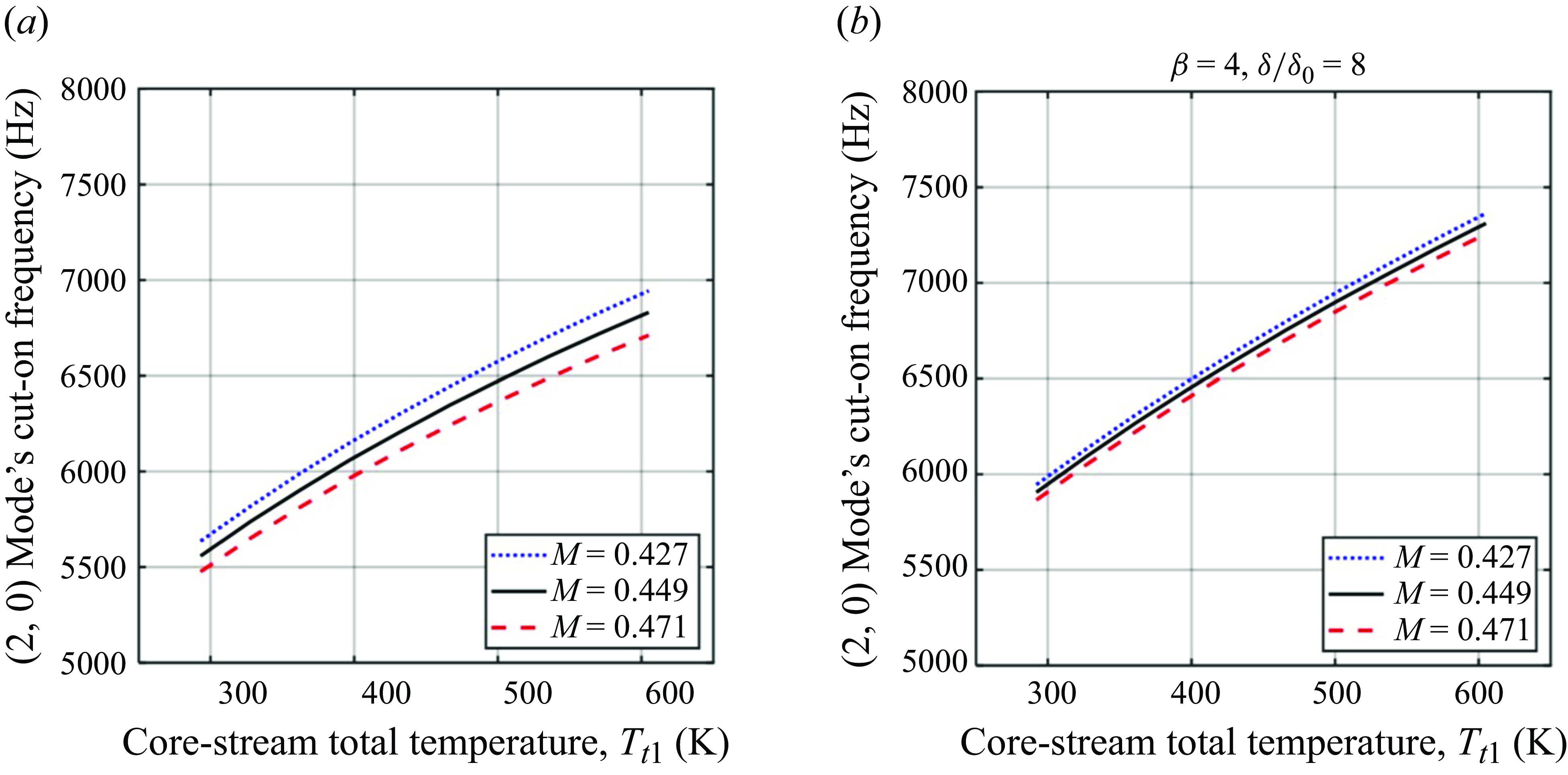
5. Conclusions
This paper has shown that the howling of an axisymmetric, model-scale internally mixed air jet originally reported by Ramsey et al. (Reference Ramsey, Mayo, Karon, Funk and Ahuja2022b
) was the result of an aeroacoustic feedback phenomenon in the nozzle’s interior. The flow around a small-radius, convex bend just upstream of the final-nozzle exit led to a pocket of locally supersonic flow that was terminated by a shock. This shock was strong enough to separate the boundary layer; however, the flow did not remain separated. Rather, a periodic separation occurred as part of a periodic SWBLI. It was observed experimentally that the periodic separation occurred at the frequency of the acoustic tones that were produced – both of which corresponded to the frequency of a natural acoustic mode of the straight section of the nozzle’s round mixing duct calculated using various models. These observations are understood as a feedback phenomenon formed between a natural acoustic mode of the nozzle interior and the periodic SWBLI. That is, energy was extracted from the motion of the gas by the SWBLI whose associated pressure fluctuations excited a natural acoustic mode of the nozzle’s interior. The SWBLI then locked-on to the natural acoustic mode. A discrepancy remains between the experiments and CFD results presented in this paper. The fluctuations present in the HRLES results exhibit an $m=0$
azimuthal order while those in the experiments exhibit an
$m=0$
azimuthal order while those in the experiments exhibit an $m=2$
azimuthal order. However, an otherwise similar phenomenon is found.
$m=2$
azimuthal order. However, an otherwise similar phenomenon is found.
Based on the success of a boundary-layer trip in suppressing the howling, it seems unlikely that a similar howling would occur in a full-scale nozzle due to thicker and more-turbulent boundary layers naturally occurring. Even so, understanding and being able to suppress the howling at model scale is important so model-scale jet-noise measurements obtained at all jet operating conditions of interest are representative of full-scale jet noise. Although this paper dealt with an internally mixed jet, it would seem that a single-stream nozzle with similar internal geometry to the nozzle studied here (i.e. a round duct section followed by a rapid contraction terminated by a small-radius, convex bend just upstream of the final exit) could produce a similar howling.
Ultimately, the howling was an unfavourable result of the nozzle’s design – that is, the nozzle contained a small-radius, convex bend in its interior wall just upstream of its final exit. Such design features have been found in prior works to produce a broadband excess noise in internally mixed nozzles equipped with lobed mixers. However, to the authors’ best knowledge, it seems that the present work was the first study to find that a periodic SWBLI may result as well. It is recommended that designers of model-scale, internally mixed nozzles take special care to avoid small-radius, convex bends just upstream of the nozzle exit. This type of nozzle is more likely to contain such convex bends than single-stream research nozzles due to a substantial area contraction being required over relatively short streamwise distances just upstream of the final-nozzle exit to achieve reasonably short ‘mixing-duct lengths.’ It is noted that internally mixed nozzles used for recent jet-noise testing at NASA (e.g. see Bridges & Wernet Reference Bridges and Wernet2021; Bridges Reference Bridges2023) eliminated issues associated with convex bends in the nozzle wall by using a purely convergent geometry, rather than including parallel walls just upstream of the final exit. Clemens & Gavin (Reference Clemens and Gavin2024) have recently shown that parallel walls at the final-nozzle exit of a model-scale internally mixed nozzle may be included with minimal locally supersonic flow, provided that the nozzle’s interior wall is carefully contoured.
We note that all frequencies presented in this paper were dimensional (in hertz). It is common to find non-dimensional frequencies in the published jet-noise literature formed using a length scale, $l$
(i.e. the nozzle’s exit diameter), and a velocity scale,
$l$
(i.e. the nozzle’s exit diameter), and a velocity scale, $U$
(i.e. the jet velocity for a Strouhal number or ambient sound speed for a Helmholtz number), characteristic of the jet. For the howling (i.e. acoustic tones) which are of greatest interest to this paper, these typical non-dimensional frequencies do not seem to provide a meaningful normalisation scheme. This has become clear in this paper, where we have shown that the howling occurred at a natural frequency of the nozzle’s mixing duct where the relevant length and velocity scales are not those in the final jet. Nonetheless, to allow the reader to readily compare this paper’s findings with other published literature, we note that the howling at
$U$
(i.e. the jet velocity for a Strouhal number or ambient sound speed for a Helmholtz number), characteristic of the jet. For the howling (i.e. acoustic tones) which are of greatest interest to this paper, these typical non-dimensional frequencies do not seem to provide a meaningful normalisation scheme. This has become clear in this paper, where we have shown that the howling occurred at a natural frequency of the nozzle’s mixing duct where the relevant length and velocity scales are not those in the final jet. Nonetheless, to allow the reader to readily compare this paper’s findings with other published literature, we note that the howling at $M_j = 0.90$
with the flow unheated occurred at a Strouhal number of approximately 0.9. As was shown in this paper, the howling occurred at a frequency that was insensitive to the jet Mach number. Thus, for lower jet Mach numbers that produced the howling (lower
$M_j = 0.90$
with the flow unheated occurred at a Strouhal number of approximately 0.9. As was shown in this paper, the howling occurred at a frequency that was insensitive to the jet Mach number. Thus, for lower jet Mach numbers that produced the howling (lower $U_j$
), the Strouhal number of the howling (
$U_j$
), the Strouhal number of the howling ( $fD_e/U_j$
) would be slightly higher – and the opposite is true for higher jet Mach numbers. No nominal Strouhal number is provided for cases with a heated core stream because are multiple length and velocity scales that are relevant, even at a given axial position.
$fD_e/U_j$
) would be slightly higher – and the opposite is true for higher jet Mach numbers. No nominal Strouhal number is provided for cases with a heated core stream because are multiple length and velocity scales that are relevant, even at a given axial position.
There are several fundamental questions which could be addressed by future research. Three topics are recommended here. First, the current understanding of the feedback phenomenon implies that the SWBLI is receptive to acoustic forcing; however, the precise details of this receptivity have not been dealt with in this paper. Further study of the SWBLI’s receptivity mechanisms is recommended for future work. Second, the sound-generation mechanism associated with the periodic SWBLI has been left unaddressed in this paper. The manner in which the flow instability excited the natural acoustic mode thus remains unclear. There are at least two possibilities. The first are upstream-travelling acoustic waves which emerge after the shock inside the nozzle vanishes during each cycle of the periodic SWBLI. These upstream-travelling waves were visible in the HRLES results animated in Supplementary Movie 3. The second are pressure disturbances associated with the massive, periodic displacement of the jet’s shear layer caused by the periodic SWBLI. Third, the SWBLI’s characteristic frequency (i.e. the frequency it would occur at in the absence of acoustic coupling) has not been determined. Further study of this is recommended for future work. This may provide insight into why coupling with one natural acoustic mode of the nozzle interior tended to be observed (i.e. as noted earlier in this paper, perhaps the SWBLI’s characteristic frequency was closer to the $(2,0)$
acoustic mode’s cut-on frequency than to others).
$(2,0)$
acoustic mode’s cut-on frequency than to others).
Supplementary movies
Supplementary movies are available at https://doi.org/10.1017/jfm.2025.10170.
Acknowledgements
Senior Research Engineer Dr A. Karon, Principal Research Engineer Dr R. Funk, Graduate Research Assistants R. Mayo and J. Larisch, and Research Engineer D. Dickey of GTRI are thanked for their support with the experimental campaign and for helpful discussions. Special thanks are due to Senior Research Engineer Dr N. Breen (GTRI) for his time spent reviewing the manuscript.
Funding
This paper appeared as a section in D.N.R.’s doctoral dissertation, and much of the work presented here was supported by the National Science Foundation Graduate Research Fellowship under Grant No. DGE-2039655. Any opinion, findings and conclusions or recommendations expressed in this material are those of the authors and do not necessarily reflect the views of the National Science Foundation. The building block for this work was the discovery of large-amplitude tones in the acoustic far field of confluent nozzles during work under FAA ASCENT Project 59B under grant GR00005737 (Program Manager: Dr S. Liu) and through a cost-sharing partnership with Gulfstream Aerospace (POC: B. Cook). The authors are grateful to GTRI for allowing the use of their facilities in completing this work.
Declaration of interests
The authors representativeort no conflict of interest.
Appendix A. A means of suppressing the howling
A boundary-layer trip was installed in the converging section of the final nozzle just upstream of the small-radius, convex bend and associated SWBLI as shown in figure 28(a). The trip was fashioned out of steel wire with 0.5-mm diameter that ran one full revolution around the nozzle’s inner wall. The wire was retained by four, roughly equally spaced rectangles of duct tape approximately 0.45-mm thick. As shown by the acoustic spectra acquired with and without the trip in figure 28(b), the addition of the trip suppressed the howling entirely. The tones and the broadband amplification of jet noise both vanished and a typical jet-noise spectrum was left behind – matching very well with the expected noise (which was obtained by scaling the $M_j$
= 0.80 jet-noise spectrum that was free of tones to
$M_j$
= 0.80 jet-noise spectrum that was free of tones to $M_j$
= 0.90).
$M_j$
= 0.90).
Boundary-layer trip for suppressing the howling: (a) nominal trip location relative to SWBLI and (b) measured effect of trip on lossless, fully corrected acoustic spectrum ( $L_e/D_e$
= 0.7,
$L_e/D_e$
= 0.7, $M_j$
= 0.90, unheated,
$M_j$
= 0.90, unheated, $\theta = 90^{\circ }$
,
$\theta = 90^{\circ }$
, $\Delta f =$
32 Hz,
$\Delta f =$
32 Hz, $R = 84.7D_e$
). (Scaled
$R = 84.7D_e$
). (Scaled $M_j$
= 0.80 spectrum from Ramsey et al. (2022b)).
$M_j$
= 0.80 spectrum from Ramsey et al. (2022b)).
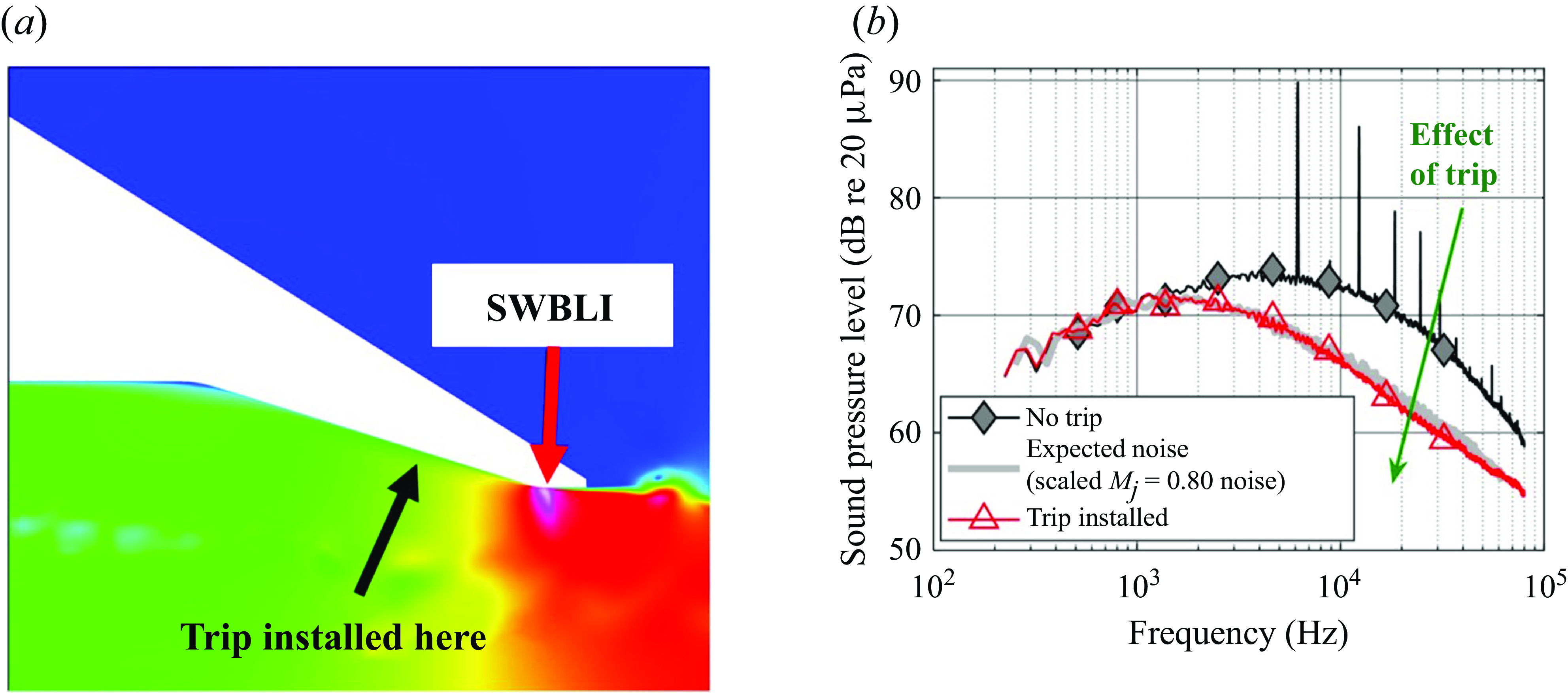
Typically, boundary-layer trips make the boundary layer thicker and more turbulent and, as discussed by Babinsky & Harvey (Reference Babinsky and Harvey2011), turbulent boundary layers are less prone to shock-induced separation than laminar ones. Therefore, the boundary layer itself is expected to be less prone to shock-induced separation with the trip in place. However, we do not wish to discount the possibility that the trip may modify the Mach-number distribution inside the nozzle. The effect of increasing the radius of curvature in a transonic, convex-corner flow has been shown by Chung et al. (Reference Chung, Chang, Chang and Lu2014) to reduce the resulting maximum Mach number (as evidenced by the wall-pressure distribution). It could be that, in the present case, a thicker boundary layer results in the high-velocity gas just outside the boundary layer being subjected to a larger-radius (i.e. less aggressive) turn than if the boundary layer was thinner and that, in a similar way to increasing a corner’s radius, the maximum Mach number would be reduced. Nonetheless, we simply state that the suppression of the howling by this trip resulted from making the boundary layer that approached the small-radius, convex bend thicker and more turbulent than what naturally developed. More detailed work on this issue would be required to better understand the potentially multi-faceted role that such changes to the incoming boundary layer have on the transonic flow around the small-radius bend.
It is noted that many tests were conducted with different boundary-layer-trip configurations. Some findings are briefly discussed here without presentation of the associated data for brevity. Firstly, it was found that the four strips of tape added to the interior of the nozzle at approximately the same locations as used for trip-ring retention did not eliminate the howling. Although the tape and the wire were of the same order of thickness, the tape alone was not sufficient. Additionally, a boundary-layer trip, which was formed by the same 0.5-mm-diameter wire which ran one-half revolution around the nozzle and was retained by three strips of tape, did not suppress the howling either. These results suggested that the boundary-layer trip must run one full revolution around the nozzle to be effective.
For completeness, we note that Zaman et al. (Reference Zaman, Dahl, Bencic and Loh2002) suppressed a different nozzle-based resonance by tripping the boundary layer upstream of a SWBLI, too.
Appendix B. Calculation of mixing duct’s natural acoustic modes in the presence of uniform flow
The cut-on frequencies of the higher-order acoustic modes of the nozzle’s round mixing duct presented in § 3.4 were found by first solving the dispersion relation for a round duct of radius $R_d$
without flow. This dispersion relation is obtained by imposing boundary conditions (boundedness on the centreline at
$R_d$
without flow. This dispersion relation is obtained by imposing boundary conditions (boundedness on the centreline at $r = 0$
and rigid wall at
$r = 0$
and rigid wall at $r = R_d$
) on the general solution to the linearised, inviscid governing equations and is given by
$r = R_d$
) on the general solution to the linearised, inviscid governing equations and is given by
 \begin{align} J'_m(\eta R_d) = 0, \end{align}
where $J'_m$
is the derivative of the Bessel function of the first kind of order
$J'_m$
is the derivative of the Bessel function of the first kind of order $m$
(the azimuthal order of the acoustic mode of interest) is an integer. The variable
$m$
(the azimuthal order of the acoustic mode of interest) is an integer. The variable $\eta$
is given by
$\eta$
is given by
 \begin{align} \eta \equiv \left ( \frac {\omega ^2}{a^2} - k^2 \right )^{1/2}, \end{align}
where $\omega$
is the angular frequency (real valued),
$\omega$
is the angular frequency (real valued), $k$
is the wavenumber along the duct’s axis (real valued) and
$k$
is the wavenumber along the duct’s axis (real valued) and $a$
is the speed of sound. The dependence of
$a$
is the speed of sound. The dependence of $\eta$
on
$\eta$
on $k$
,
$k$
, $\omega$
and
$\omega$
and $a$
is implied throughout. Equation (B1) may be solved numerically or via use of tabulated zeros of
$a$
is implied throughout. Equation (B1) may be solved numerically or via use of tabulated zeros of $J'_m$
. Tabulated values were used here and
$J'_m$
. Tabulated values were used here and $k$
was set to zero to solve for the cut-on frequencies. Then, to account for the effect of a uniform mean flow, the calculated cut-on frequencies were scaled by
$k$
was set to zero to solve for the cut-on frequencies. Then, to account for the effect of a uniform mean flow, the calculated cut-on frequencies were scaled by $\sqrt {1-M^2}$
(e.g. see Morfey Reference Morfey1971), where
$\sqrt {1-M^2}$
(e.g. see Morfey Reference Morfey1971), where $M$
is the Mach number of the mean flow. In calculating
$M$
is the Mach number of the mean flow. In calculating $M$
, uniform flow was assumed throughout the nozzle and the area consumed by the core-nozzle lip was removed from the mixing-duct area. Isentropic flow equations were used to estimate
$M$
, uniform flow was assumed throughout the nozzle and the area consumed by the core-nozzle lip was removed from the mixing-duct area. Isentropic flow equations were used to estimate $M$
and the static temperature inside the mixing duct. Values of
$M$
and the static temperature inside the mixing duct. Values of $T_{t1} = T_{t2} = 294$
K were assumed. The dispersion relation for a flow-containing duct could have been dealt with directly; however, scaling the cut-on frequencies following Morfey (Reference Morfey1971) provides an identical result in a simple manner.
$T_{t1} = T_{t2} = 294$
K were assumed. The dispersion relation for a flow-containing duct could have been dealt with directly; however, scaling the cut-on frequencies following Morfey (Reference Morfey1971) provides an identical result in a simple manner.
Appendix C. Dispersion relation for dual-stream vortex-sheet model
The dispersion relation for a ducted, axisymmetric vortex-sheet model (introduced in § 4.2) can be found in the work of Ahuja et al. (Reference Ahuja, Massey, Fleming, Tam and III1992), for example, with salient details outlined here for completeness. Where a subscript $i$
appears in this appendix, it may take a value of
$i$
appears in this appendix, it may take a value of $1$
to designate the core stream or
$1$
to designate the core stream or $2$
to designate the bypass stream, with
$2$
to designate the bypass stream, with $i$
taking the same value in all places it appears in a given expression. The analysis assumes compressible, parallel flow of an inviscid and non-heat-conducting fluid. Following the now-standard procedure that has been discussed by Ahuja et al. (Reference Ahuja, Massey, Fleming, Tam and III1992) (also see Tam & Hu (Reference Tam and Hu1989) and Morris (Reference Morris2010), among others) after linearising the governing equations, introducing a normal-mode ansatz, and imposing interface conditions (continuity of pressure and vortex-sheet displacement at
$i$
taking the same value in all places it appears in a given expression. The analysis assumes compressible, parallel flow of an inviscid and non-heat-conducting fluid. Following the now-standard procedure that has been discussed by Ahuja et al. (Reference Ahuja, Massey, Fleming, Tam and III1992) (also see Tam & Hu (Reference Tam and Hu1989) and Morris (Reference Morris2010), among others) after linearising the governing equations, introducing a normal-mode ansatz, and imposing interface conditions (continuity of pressure and vortex-sheet displacement at $r = R_1$
) and boundary conditions (boundedness of pressure at the centreline of the duct and impermeable, rigid wall at
$r = R_1$
) and boundary conditions (boundedness of pressure at the centreline of the duct and impermeable, rigid wall at $r = R_2$
), the dispersion relation is obtained as
$r = R_2$
), the dispersion relation is obtained as
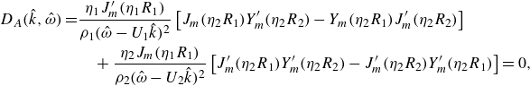 \begin{align} D_A(\hat {k},\hat {\omega }) = & \dfrac {\eta _1J'_m(\eta _1R_1)}{\rho _1(\hat {\omega } - U_1\hat {k})^2}\left [ J_m(\eta _2R_1) Y'_m(\eta _2R_2) - Y_m(\eta _2R_1) J'_m(\eta _2R_2) \right ] \nonumber \\ & \quad + \dfrac {\eta _2J_m(\eta _1R_1)}{\rho _2({\hat {\omega }} - U_2\hat {k})^2}\left [ J'_m(\eta _2R_1) Y'_m(\eta _2R_2) - J'_m(\eta _2R_2) Y'_m(\eta _2R_1) \right ] = 0, \end{align}
where $\hat {k}$
,
$\hat {k}$
, $\hat {\omega }$
and
$\hat {\omega }$
and $m$
are the complex wavenumber, complex angular frequency and azimuthal periodicity of a disturbance imposed on the vortex sheet,
$m$
are the complex wavenumber, complex angular frequency and azimuthal periodicity of a disturbance imposed on the vortex sheet, $\rho _{i}$
and
$\rho _{i}$
and $U_{i}$
are the mean density and axial velocity,
$U_{i}$
are the mean density and axial velocity, $J_m$
and
$J_m$
and $Y_m$
are Bessel functions of the first and second kind of order
$Y_m$
are Bessel functions of the first and second kind of order $m$
, primes denote differentiation with respect to the Bessel-function arguments and
$m$
, primes denote differentiation with respect to the Bessel-function arguments and
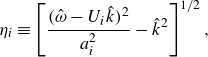 \begin{align} \eta _i \equiv \left [ \frac {({\hat {\omega }} - U_i\hat {k})^2}{a_i^2} - \hat {k}^2 \right ]^{1/2}, \end{align}
where $a_i$
is the speed of sound. The dependence of
$a_i$
is the speed of sound. The dependence of $\eta _i$
on
$\eta _i$
on $\hat {k}$
,
$\hat {k}$
, $\hat {\omega }$
,
$\hat {\omega }$
, $a$
and
$a$
and $U$
is implied throughout. The branch cut for
$U$
is implied throughout. The branch cut for $\eta _i$
was taken along the negative real axis. For a specified
$\eta _i$
was taken along the negative real axis. For a specified $m$
and set of flow conditions (which specify
$m$
and set of flow conditions (which specify $U_i$
,
$U_i$
, $a_i$
,
$a_i$
, $\rho _i$
), pairs of
$\rho _i$
), pairs of $\hat {k}$
and
$\hat {k}$
and $\hat {\omega }$
are sought which satisfy equationC1. These
$\hat {\omega }$
are sought which satisfy equationC1. These $\hat {k}-\hat {\omega }$
pairs describe the waves supported by the dual-stream flow.
$\hat {k}-\hat {\omega }$
pairs describe the waves supported by the dual-stream flow.
Appendix D. Dispersion relation for tri-stream vortex-sheet model
The procedure for obtaining the dispersion relation for the tri-stream vortex-sheet model (introduced in § 4.3) is a natural extension of that required for the dual-stream vortex-sheet model, and a detailed outline is provided here. Where a subscript $i$
appears in what follows, it may take a value of
$i$
appears in what follows, it may take a value of $1$
to designate the core stream,
$1$
to designate the core stream, $2$
to designate the bypass stream, or
$2$
to designate the bypass stream, or $W$
to designate the wake region, with
$W$
to designate the wake region, with $i$
taking the same value in all places it appears in a given expression. The governing equation for the disturbance pressure is the same in each of the three regions of the flow. This equation is (see Tam & Hu (Reference Tam and Hu1989) and Morris (Reference Morris2010), among others)
$i$
taking the same value in all places it appears in a given expression. The governing equation for the disturbance pressure is the same in each of the three regions of the flow. This equation is (see Tam & Hu (Reference Tam and Hu1989) and Morris (Reference Morris2010), among others)
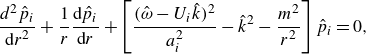 \begin{align} \frac {d^2 \hat {p}_{i}}{{\rm d} r^2} + \frac {1}{r}\frac {{\rm d} \hat {p}_{i}}{{\rm d}r} + \left [ \frac {(\hat {\omega } - U_{i}\hat {k})^2}{a_{i}^2} - \hat {k}^2 - \frac {m^2}{r^2} \right ]\hat {p}_{i} = 0, \end{align}
where $\hat {p}_i$
is the radial profile of disturbance pressure and
$\hat {p}_i$
is the radial profile of disturbance pressure and $r$
is the radial coordinate (all other variables were defined in Appendix C). The disturbance-pressure profiles which satisfy this governing equation are of the form
$r$
is the radial coordinate (all other variables were defined in Appendix C). The disturbance-pressure profiles which satisfy this governing equation are of the form
 \begin{align} \hat {p}_{i} = A_{i}J_m(\eta _{i} r) + B_{i}Y_m(\eta _{i} r), \end{align}
where $A_i$
and
$A_i$
and $B_i$
are constants to be determined. Given this general solution, there are a total of six unknown coefficients (
$B_i$
are constants to be determined. Given this general solution, there are a total of six unknown coefficients ( $A_i$
and
$A_i$
and $B_i$
corresponding to each of the core, wake, and bypass streams) that need to be selected in accordance with the boundary conditions at the duct’s wall/centreline and interfacial conditions that apply at the interfaces between the three streams.
$B_i$
corresponding to each of the core, wake, and bypass streams) that need to be selected in accordance with the boundary conditions at the duct’s wall/centreline and interfacial conditions that apply at the interfaces between the three streams.
First, consider the boundary conditions. The pressure along the centreline of the duct must be bounded, and therefore
 \begin{align} \hat {p}_1 = A_1 J_m(\eta _1 r) \end{align}
(i.e. there can be no contribution from $Y_m$
, so
$Y_m$
, so $B_1 = 0$
). Then, assuming the duct containing the flow to be impermeable and rigid, the radial gradient of the disturbance pressure must be zero at the wall of the duct (
$B_1 = 0$
). Then, assuming the duct containing the flow to be impermeable and rigid, the radial gradient of the disturbance pressure must be zero at the wall of the duct ( $r = R_2$
)
$r = R_2$
)
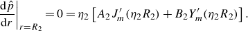 \begin{align} \left . \frac {{\rm d}\hat {p}}{{\rm d}r} \right |_{r = R_2} = 0 = \eta _2\left [A_2J_m'(\eta _2 R_2) + B_2Y_m'(\eta _2 R_2) \right ]. \end{align}
This allows for either $A_2$
or
$A_2$
or $B_2$
to be eliminated from the expression for
$B_2$
to be eliminated from the expression for $\hat {p}_2$
. We chose to eliminate
$\hat {p}_2$
. We chose to eliminate $B_2$
.
$B_2$
.
Now, the interfacial conditions are imposed. At the interface between the core and wake streams, continuity of normal stress is enforced as $\left . \hat {p}_{1} \right |_{r = R_1} = \left . \hat {p}_{W} \right |_{r = R_1}$
. Written in terms of the disturbance-pressure expressions, this becomes
$\left . \hat {p}_{1} \right |_{r = R_1} = \left . \hat {p}_{W} \right |_{r = R_1}$
. Written in terms of the disturbance-pressure expressions, this becomes
 \begin{align} A_{1}J_m(\eta _{1} R_1) = A_{W}J_m(\eta _{W} R_1) + B_{W}Y_m(\eta _{W} R_1), \end{align}
which allows for $A_1$
to be eliminated from the expression for
$A_1$
to be eliminated from the expression for $\hat {p}_1$
. In summary, we now have the following expressions for the disturbance-pressure profiles:
$\hat {p}_1$
. In summary, we now have the following expressions for the disturbance-pressure profiles:
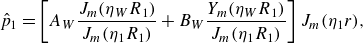 \begin{align} \hat {p}_1 = \left [ A_{W}\frac {J_m(\eta _{W} R_1)}{J_m(\eta _{1} R_1)} + B_{W}\frac {Y_m(\eta _{W} R_1)}{J_m(\eta _{1} R_1)} \right ] J_m(\eta _1 r), \\[-24pt] \nonumber \end{align}
 \begin{align} \hat {p}_W = A_{W}J_m(\eta _{W} r) + B_{W}Y_m(\eta _{W} r), \\[-24pt] \nonumber \end{align}
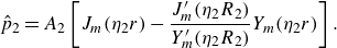 \begin{align} \hat {p}_{2} = A_{2}\left [J_m(\eta _{2} r) - \frac {J_m'(\eta _2R_2)}{Y_m'(\eta _2R_2)}Y_m(\eta _{2} r) \right ]. \end{align}
These three equations involve three unknowns: $A_W$
,
$A_W$
, $B_W$
and
$B_W$
and $A_2$
.
$A_2$
.
Three more equations are needed, and are obtained by imposing continuity of normal stress at the wake/bypass interface and continuity of vortex-sheet displacement (e.g. see Tam & Hu (Reference Tam and Hu1989) and Morris (Reference Morris2010) among others) at both of the core/wake and wake/bypass interfaces. These conditions are expressed in terms of the disturbance-pressure profiles as
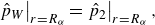 \begin{align} \left . \hat {p}_W \right |_{r = R_{\alpha }} = \left . \hat {p}_2 \right |_{r = R_{\alpha }} , \\[-24pt] \nonumber \end{align}
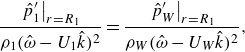 \begin{align} \frac { \left .\hat {p}_1' \right |_{r = R_1}}{\rho _1 (\hat {\omega } - U_1\hat {k})^2} = \frac { \left .\hat {p}_W' \right |_{r = R_1}}{\rho _W (\hat {\omega } - U_W\hat {k})^2} , \\[-24pt] \nonumber \end{align}
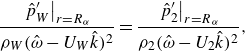 \begin{align} \frac { \left .\hat {p}_W' \right |_{r = R_{\alpha }}}{\rho _W (\hat {\omega } - U_W\hat {k})^2} = \frac { \left .\hat {p}_2' \right |_{r = R_{\alpha }}}{\rho _2 (\hat {\omega } - U_2\hat {k})^2} ,\end{align}
where primes denote derivatives with respect to the radial coordinate. It is left to the reader to write out these three interfacial conditions in terms of the three $\hat {p}_i$
expressions given above. Following Ahuja et al. (Reference Ahuja, Massey, Fleming, Tam and III1992), the dispersion relation may be found by writing the three resulting equations in matrix form and taking the determinant of the matrix of coefficients of
$\hat {p}_i$
expressions given above. Following Ahuja et al. (Reference Ahuja, Massey, Fleming, Tam and III1992), the dispersion relation may be found by writing the three resulting equations in matrix form and taking the determinant of the matrix of coefficients of $A_W$
,
$A_W$
, $B_W$
and
$B_W$
and $A_2$
. The dispersion relation is obtained as
$A_2$
. The dispersion relation is obtained as
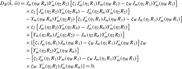 \begin{align} D_B(\hat {k},\hat {\omega })& = J_m(\eta _WR_\alpha )Y'_m(\eta _2R_2) \left [ \zeta _1J_m'(\eta _1R_1)Y_m(\eta _WR_1) - \zeta _WJ_m(\eta _1R_1)Y'_m(\eta _WR_1) \right ] \nonumber \\ & \quad \times \zeta _2 \left [ J_m'(\eta _2R_2)Y_m'(\eta _2R_\alpha ) - J'_m(\eta _2R_\alpha )Y'_m(\eta _2R_2) \right ] \nonumber \\ & \quad - Y_m(\eta _WR_\alpha )Y'_m(\eta _2R_2) \left [ \zeta _1J_m'(\eta _1R_1)J_m(\eta _WR_1) - \zeta _WJ_m(\eta _1R_1)J'_m(\eta _WR_1) \right ] \nonumber \\ & \quad \times \zeta _2 \left [ J_m'(\eta _2R_2)Y_m'(\eta _2R_\alpha ) - J'_m(\eta _2R_\alpha )Y'_m(\eta _2R_2) \right ] \nonumber \\ & \quad + \left [ Y_m(\eta _2R_\alpha )J'_m(\eta _2R_2) - J_m(\eta _2R_\alpha )Y_m'(\eta _2R_2) \right ] \nonumber \\ & \quad \times \Bigl \{ \left [ \zeta _1J_m'(\eta _1R_1)J_m(\eta _WR_1) - \zeta _WJ_m(\eta _1R_1)J'_m(\eta _WR_1) \right ] \zeta _W\nonumber \\ & \quad \times \left [ Y_m'(\eta _2R_2)Y_m'(\eta _WR_\alpha )\right ] \nonumber \\ & \quad - \left . \left [ \zeta _1J_m'(\eta _1R_1)Y_m(\eta _WR_1) - \zeta _WJ_m(\eta _1R_1)Y'_m(\eta _WR_1) \right ] \right . \nonumber \\ & \quad \times \zeta _W \left . Y_m'(\eta _2R_2)J_m'(\eta _WR_\alpha )\right . \Bigr \} = 0, \end{align}
Magnitude of the pressure eigenfunction associated with $(2,0)$
acoustic mode of mixing duct at its cut-on frequency calculated using (a, c) dual-stream and (b, d) tri-stream vortex-sheet models (
$(2,0)$
acoustic mode of mixing duct at its cut-on frequency calculated using (a, c) dual-stream and (b, d) tri-stream vortex-sheet models ( $M = 0.449, T_{t2} = 293$
K): (a, b) unheated flow and (c, d)
$M = 0.449, T_{t2} = 293$
K): (a, b) unheated flow and (c, d) $T_{t1} = 600$
K. Dashed curve shows uniform-flow result.
$T_{t1} = 600$
K. Dashed curve shows uniform-flow result.
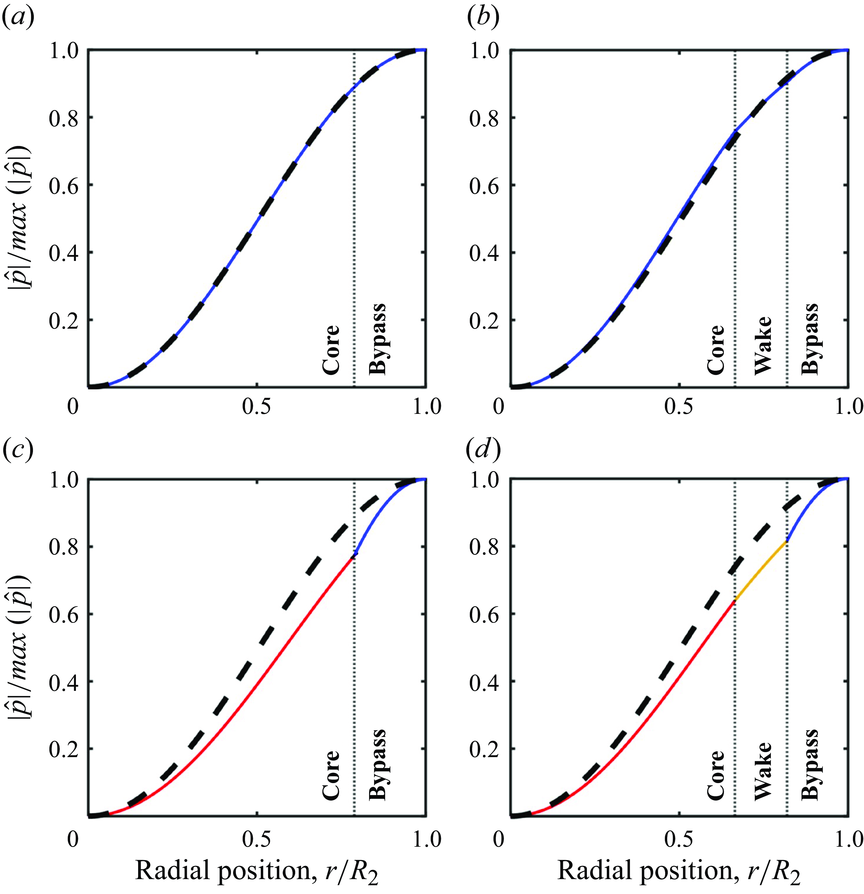
where $ \zeta _i \equiv \eta _i / [\rho _i(\hat {\omega }-U_i\hat {k})^2 ]$
. For a specified
$ \zeta _i \equiv \eta _i / [\rho _i(\hat {\omega }-U_i\hat {k})^2 ]$
. For a specified $m$
and set of flow conditions (which specify
$m$
and set of flow conditions (which specify $U_i$
,
$U_i$
, $a_i$
,
$a_i$
, $\rho _i$
), pairs of
$\rho _i$
), pairs of $\hat {k}$
and
$\hat {k}$
and $\hat {\omega }$
are sought which satisfy equation (D12). These
$\hat {\omega }$
are sought which satisfy equation (D12). These $\hat {k}-\hat {\omega }$
pairs describe the waves supported by the three-stream flow.
$\hat {k}-\hat {\omega }$
pairs describe the waves supported by the three-stream flow.
Appendix E. Pressure eigenfunctions of the $\boldsymbol{(2,0)}$
acoustic mode with non-uniform flow
$\boldsymbol{(2,0)}$
acoustic mode with non-uniform flow

In figure 29, a few different examples of the $(2,0)$
acoustic mode’s pressure eigenfunction are shown. In each of the four plots, there are two curves. The solid curve corresponds to the
$(2,0)$
acoustic mode’s pressure eigenfunction are shown. In each of the four plots, there are two curves. The solid curve corresponds to the $(2,0)$
mode at its cut-on frequency obtained via vortex-sheet model calculations corresponding to the cut-on frequency of the mode. The dashed curve corresponds to the classical
$(2,0)$
mode at its cut-on frequency obtained via vortex-sheet model calculations corresponding to the cut-on frequency of the mode. The dashed curve corresponds to the classical $(2,0)$
acoustic mode of a duct in the presence of uniform flow. All calculations assume
$(2,0)$
acoustic mode of a duct in the presence of uniform flow. All calculations assume $M=0.449$
. Generally, unlike ducts containing uniform flows, acoustic modes of ducts containing non-uniform flows exhibit frequency-dependent pressure eigenfunctions. This has been discussed in § 5.3 of Ramsey (Reference Ramsey2024), for example. In figure 29(a), the dual-stream vortex-sheet model’s result for unheated flow is shown. Because the core and bypass streams have the same properties, this is identically a case of uniform flow and the two curves overlap. In figure 29(b), the same is shown for the tri-stream model. Note that the mean flow is not uniform in this case because the wake was taken to have zero mean velocity, and there are some small differences between the two curves. Figures 29(c) and 29(d) parallel figures 29(a) and 29(b) but with the core stream at
$M=0.449$
. Generally, unlike ducts containing uniform flows, acoustic modes of ducts containing non-uniform flows exhibit frequency-dependent pressure eigenfunctions. This has been discussed in § 5.3 of Ramsey (Reference Ramsey2024), for example. In figure 29(a), the dual-stream vortex-sheet model’s result for unheated flow is shown. Because the core and bypass streams have the same properties, this is identically a case of uniform flow and the two curves overlap. In figure 29(b), the same is shown for the tri-stream model. Note that the mean flow is not uniform in this case because the wake was taken to have zero mean velocity, and there are some small differences between the two curves. Figures 29(c) and 29(d) parallel figures 29(a) and 29(b) but with the core stream at $T_{t1} = 600$
K. With this departure from uniform flow (or nearly uniform flow, in the case of the tri-stream model including the wake), the pressure eigenfunctions exhibit more appreciable differences from those of uniform flows.
$T_{t1} = 600$
K. With this departure from uniform flow (or nearly uniform flow, in the case of the tri-stream model including the wake), the pressure eigenfunctions exhibit more appreciable differences from those of uniform flows.


 Open access