





1. Introduction
Turbulent heat transfer is an important physical process frequently observed in nature and in industrial applications such as atmospheric convection, heat exchangers and gas turbines. In particular, accurate estimation of the heat flux at the solid boundary is essential for better design of heat-exchanging devices. The close analogy between heat and momentum, known as the Reynolds analogy, suggests a strong similarity between heat flux and shear stress at the wall. For the given shear stress field, however, the distribution of heat flux highly depends on Prandtl numbers ( $Pr = \nu / \alpha$; $\nu$ and $\alpha$ are the kinematic viscosity and thermal diffusivity, respectively), indicating that the relationship between the shear stress and heat flux is not simple. This complicated relationship makes it more difficult to predict heat transfer than shear stress. However, the detailed effect of the Prandtl number on heat transfer has not been well investigated. In practice, the prediction of turbulent heat transfer is usually performed using turbulence models such as the Reynolds-averaged Navier–Stokes (RANS) model, but its accuracy is still not satisfactory compared with the relatively well-predicted skin friction (Hoda & Acharya Reference Hoda and Acharya1999; Coletti et al. Reference Coletti, Benson, Ling, Elkins and Eaton2013).
Several attempts have been made to investigate turbulent heat transfer using direct numerical simulations (DNS). For example, Antonia, Krishnamoorthy & Fulachier (Reference Antonia, Krishnamoorthy and Fulachier1988), Kim & Moin (Reference Kim and Moin1989), Kasagi, Tomita & Kuroda (Reference Kasagi, Tomita and Kuroda1992) studied the temperature fields with  $Pr$ in turbulent channel flow and reported a strong correlation between the streamwise velocity and temperature fluctuations near the wall. Similarly, Abe & Antonia (Reference Abe and Antonia2009) found that near the wall, the correlation between the velocity and scalar fluctuations peaks when the pressure fluctuation effect is small. Abe, Kawamura & Matsuo (Reference Abe, Kawamura and Matsuo2004) showed close similarity between the streamwise wall-shear stress and wall-normal heat flux fluctuations. They also observed the space–time correlation of the surface heat flux and found that the correlation for $Pr=0.025$ has a larger value than that for $Pr=0.71$ at large separations, indicating the effect of large-scale structures. Kasagi & Ohtsubo (Reference Kasagi and Ohtsubo1993) presented that thermal streaks for low Prandtl numbers have larger spacing than those for high Prandtl numbers in the spanwise direction. Kawamura et al. (Reference Kawamura, Ohsaka, Abe and Yamamoto1998) and Kawamura, Abe & Matsuo (Reference Kawamura, Abe and Matsuo1999) examined statistically the effect of the Prandtl number, showing that the peak of the temperature variance is observed closer to the wall with increasing $Pr$. Na & Hanratty (Reference Na and Hanratty2000) investigated the limiting behaviour of the passive scalar with higher $Pr$ near the wall. They reported that the contribution of high wavenumbers increases in the energy spectra of temperature fluctuations with increasing $Pr$. As such, the effect of the Prandtl number has been investigated, but the observation of local heat flux with the Prandtl number has not been sufficiently performed because it is mostly limited to the conventional statistical approach. The turbulent transport mechanism of heat and momentum near the wall occurs locally and intermittently owing to the presence of near-wall vortical structures. The dissimilarity between the heat flux and streamwise shear stress was evident in some regions, although there was a high correlation between them. Therefore, we focus on revealing the complicated relationship between the local heat flux and wall-shear stresses by considering the Prandtl number effect. For this purpose, we employ deep learning (DL) to find a nonlinear mapping function between instantaneous fields with high prediction accuracy. We analyse the trained model embedding the Prandtl number to identify the underlying physics.
The applicability of a neural network (NN) to learn the nonlinear relationship between turbulent variables has been attempted previously. In a pioneering study, Lee et al. (Reference Lee, Kim, Babcock and Goodman1997) applied a shallow NN for the prediction and control of near-wall turbulence using wall-shear stress information, although it was confined to finding a simple relationship owing to the limitations of the computational resources of the time. Recently, with the development of computing hardware, data-driven algorithms and their open-source libraries, the learning of highly complex phenomena using deep neural networks (DNN) has become feasible. For the purpose of prediction and control, there have been studies that trained the nonlinearity between the near-wall variables. Güemes, Discetti & Ianiro (Reference Güemes, Discetti and Ianiro2019) and Güastoni et al. (Reference Güastoni, Guemes, Ianiro, Discetti, Schlatter, Azizpour and Vinuesa2021) used a convolutional neural network (CNN)-based model to predict flow fields from wall-shear stresses, and showed that the model can learn nonlinear effects of the near-wall mechanism. Han & Huang (Reference Han and Huang2020) and Park & Choi (Reference Park and Choi2020) proposed a controller based on CNN that predicts the wall-normal velocity using wall signals for skin-friction drag reduction. For high-resolution reconstruction, studies have addressed the relationship between large-scale and small-scale fields. Fukami, Fukagata & Taira (Reference Fukami, Fukagata and Taira2019) showed that high-resolution data can be reconstructed from filtered DNS data of homogeneous isotropic turbulence using CNN. Kim et al. (Reference Kim, Kim, Won and Lee2021) demonstrated the usefulness of generative adversarial networks (GANs)-based unsupervised DL by applying it to the problem of reconstructing DNS-quality data from large-eddy simulation (LES) data in turbulent channel flow. Similarly, Güemes et al. (Reference Güemes, Discetti, Ianiro, Sirmacek, Azizpour and Vinuesa2021) demonstrated the possibility of generating wall-parallel flow fields from coarse wall information using GANs. For LES modelling, there are studies that have learned the relationship between resolved scale and sub-grid scale (SGS) fields. Maulik et al. (Reference Maulik, San, Rasheed and Vedula2019) developed a DNN model that predicts the SGS stress based on local resolved velocity gradient information in two-dimensional turbulence. Similarly, DL models for SGS have been applied to various canonical flows (Gamahara & Hattori Reference Gamahara and Hattori2017; Wang et al. Reference Wang, Luo, Li, Tan and Fan2018; Xie et al. Reference Xie, Wang, Li and Ma2019; Portwood et al. Reference Portwood, Nadiga, Saenz and Livescu2020; Kim et al. Reference Kim, Kim, Kim and Lee2022). In addition, many studies have been conducted in fields such as RANS modelling (Ling, Kurzawski & Templeton Reference Ling, Kurzawski and Templeton2016; Parish & Duraisamy Reference Parish and Duraisamy2016; Wang, Wu & Xiao Reference Wang, Wu and Xiao2017) and dynamic prediction (Srinivasan et al. Reference Srinivasan, Guastoni, Azizpour, Schlatter and Vinuesa2019; Kim & Lee Reference Kim and Lee2020a; Raissi, Yazdani & Karniadakis Reference Raissi, Yazdani and Karniadakis2020; Lee & You Reference Lee and You2021), among others (see details in review papers Kutz Reference Kutz2017; Brenner, Eldredge & Freund Reference Brenner, Eldredge and Freund2019; Duraisamy, Iaccarino & Xiao Reference Duraisamy, Iaccarino and Xiao2019; Brunton, Noack & Koumoutsakos Reference Brunton, Noack and Koumoutsakos2020). As explained, DL performed well in discovering the interrelationship between the input and output in various turbulence problems, but there are still unresolved fundamental issues such as understanding how DL learns turbulence, what characteristics of turbulence DL learns, and which information is essential for prediction. In most applications, owing to complicated network structures, the interpretability of the trained network is limited.
Recently, a few attempts have been made to investigate the interpretability of DL with embedded turbulence features. Jagodinski, Zhu & Verma (Reference Jagodinski, Zhu and Verma2020) reported that a three-dimensional CNN is able to predict the intensity of ejection events in wall-bounded turbulence, and the model was able to discover critical regions for dynamics prediction. Lu, Kim & Soljačić (Reference Lu, Kim and Soljačić2020) applied a variational autoencoder to spatiotemporal systems governed by partial differential equations. They demonstrated that the model can extract interpretable physical parameters from the data of the dynamical system as a latent vector. In our previous work (Kim & Lee Reference Kim and Lee2020b), we demonstrated that a CNN can predict the local surface heat flux at  $Pr=0.71$ from the wall-shear stresses and pressure in a turbulent channel flow. We observed the gradient maps obtained through the trained CNN, and found essential parts of the input information for the prediction of the local heat flux. The interpretable DL model can help provide a framework that can discover unknown physical phenomena from data. In addition, an interpretation of DL would play a very important role in improving the learning performance and in providing guidance for DL construction, such as hyperparameter optimization.
In this study we applied a conditional generative adversarial network (cGAN) (Mirza & Osindero Reference Mirza and Osindero2014) combined with a decomposition algorithm to predict the surface heat flux for various  $Pr$ values from the wall-shear stresses in turbulent channel flow. In addition, we analysed the effect of the Prandtl number using the gradient map between the local heat flux and shear stresses through the interpretation of the trained model. In §§ 2.1 and 2.2, the numerical procedures for turbulence heat transfer and methodology for the decomposition of the physical parameter effect are presented. In § 3.1 we present the performance of the cGAN with a decomposition algorithm for predicting the surface heat flux for various $Pr$ values. In § 3.2 we analyse the physical nonlinear correlation between the wall-shear stresses and local heat flux for $Pr$ using a gradient map obtained from the trained model for the interpretation of DL. In § 3.3 we present the decomposed surface heat flux, $Pr$-dependence and $Pr$-independent features, using the decomposition algorithm and observe the decomposed surface heat flux to identify the effect of $Pr$. Finally, in § 4 the interpretability of DL for the effects of physical parameters is discussed, with concluding remarks.
2. Methodology
2.1. Data generation for training
To collect datasets for training the DL model, DNS of turbulent channel flow with passive temperature were performed for various values of  $Pr$. The mean flow in the streamwise direction is driven by a constant pressure gradient. Constant temperature and no-slip conditions were imposed on both walls, and periodic boundary conditions were used in the horizontal directions. The governing equations are the continuity, incompressible Navier–Stokes and energy equations, i.e.
 $$\begin{gather} \frac{\partial u_i}{\partial x_i} = 0, \end{gather}$$
 $$\begin{gather}\frac{\partial u_i }{\partial t} + {u_j}\frac{\partial u_i }{\partial x_j} ={-}\frac{\partial p }{\partial x_i} + \frac{1 }{Re_\tau}\frac{\partial^2{u_i} }{\partial x_j \partial x_j}, \end{gather}$$
 $$\begin{gather}\frac{\partial T}{\partial t} + {u_j}\frac{\partial T }{\partial x_j} = \frac{1}{PrRe_\tau}\frac{\partial^2{T}}{\partial x_j \partial x_j}, \end{gather}$$
where the equations are non-dimensionalized by the channel half-width  $\delta$, friction velocity $u_{\tau }$ and temperature difference $\Delta T$ between the top and bottom walls. Here $x_1 (x)$, $x_2 (y)$ and $x_3 (z)$ denote the streamwise, wall-normal and spanwise directions, respectively; $u_1 (u)$, $u_2 (v)$ and $u_3 (w)$ denote the corresponding velocity components. The dimensionless parameters are the Prandtl number and the friction Reynolds number ( $Re_\tau = u_\tau \delta / \nu$), which was fixed at 180.
A pseudo-spectral method using Fourier expansion in the horizontal direction and a central difference scheme in the wall-normal direction were used for spatial discretization. The second-order Adams–Bashforth and Crank–Nicolson schemes were applied for the temporal integration of the nonlinear and viscous terms, respectively. Simulation parameters, such as the domain size ( $L_x\times L_y \times L_z$) and the number of grid points ( $N_{x} \times N_{y} \times N_{z}$) after dealising are summarized in table 1. The resolution effect in the horizontal and wall-normal directions was verified through a test for the highest $Pr (= 7)$, with a focus only on the wall quantities. When we tested two horizontal resolutions, $(\Delta x^+, \Delta z^+) = (11.78, 5.89)$, which was used for high Prandtl numbers in our paper, and $(\Delta x^+, \Delta z^+) = (8.83, 4.42)$, there was no meaningful difference in time-averaged statistics such as $Nu$, root mean square (r.m.s.), skewness and flatness of the surface heat flux. Furthermore, through tests with two wall-normal grids, $N_y = 129$ and 257, in the Chebyshev expansion, we found that the energy spectrum of the surface heat flux is almost identical for the two cases. It indicates that present grid resolutions are fine enough for the wall information we are interested in.
Simulation parameters for DNS.

Direct numerical simulation data are divided into training, validation and testing data. The testing data are sufficiently decorrelated from the training data. We collected the streamwise wall-shear stress  $\partial u/\partial y|_{y=0}$ ( $=\tau _{w,x}$) and spanwise wall-shear stress $\partial w/\partial y|_{y=0}$ ( $=\tau _{w,z}$) as input data for DL. The surface heat flux $\partial T/\partial y|_{y=0}$ ( $=q_{w}$) for various $Pr$ were used as target outputs. To use the same amount of information for all $Pr$ in the training process of DL, spectral interpolation was applied to the DNS data for $Pr=2-7$. For all $Pr$, the number of grids of the preprocessed data are $128 \times 128$ in $x,z$ directions, and the spatial resolution $(\Delta x^+,\Delta z^+) = (17.67, 8.84)$.
2.2. Deep learning model
In this study we use a cGAN with a novel algorithm that can decompose the effect of the Prandtl number for the prediction and interpretation of the surface heat flux. A cGAN is a modified model of GAN proposed by Goodfellow et al. (Reference Goodfellow, Pouget-Abadie, Mirza, Xu, Warde-Farley, Ozair, Courville and Bengio2014), which imposes constraints on the discriminator by applying auxiliary information as a condition. The cGAN consists of two networks, a generator ( $G$) and a discriminator ( $D$), and it is trained by making the two networks compete against each other. In image-to-image generation problems, the generator generates a fake image that is similar to the target image from the input image. In our problem, the input data are the wall-shear stresses and Prandtl number, and the fake image is the surface heat flux generated by the generator, and the target image is the surface heat flux from DNS. The discriminator distinguishes between fake and real images and returns the probability value between 0 and 1. The input data are used as additional input to the discriminator for conditioning, and this constraint allows the generator to produce an output image that is dependent on the input image. Finally, we obtain a generator that yields a fake image similar to the real image while being dependent on the input data. This process can be described as a min/max problem, and the loss function used for training is
 \begin{equation} \min_{G} \max_{D}\mathcal{L}_{cGAN} = \mathbb{E}_{y\sim P_{Y}}[\log D(y|x)] + \mathbb{E}_{x\sim P_{X}}[\log(1-D(G(x)|x))], \end{equation}
where  $\mathbb {E}$ denotes expectation, and $Y$ is the real image set and $y\sim P_{Y}$ is $y$ sampled from the real image distribution; $X$ is the input image set, and $x\sim P_{X}$ is $x$ sampled from the input image distribution; $x$ is the input data of the generator (G) and the additional input data to impose constraints on the discriminator; $G(x)$ is the fake image generated by the generator and $D(G(x)|x)$ is its probability; $D(y|x)$ is the probability value for the real image, to which the conditions are applied. During the cGAN training process, the generator ( $G$) generates fake images similar to the real image; thus, $D(G(x)|x)$ is expected to return the largest probability value possible. On the other hand, the discriminator ( $D$) distinguishes even minor differences between real and fake images, and thus, $D(G(x)|x)$ is expected to return as small a value as possible. As a result, the training parameters of the generator are learned in the direction where $\log (1-D(G(x)|x))$ is minimized, and those of the discriminator are trained in the direction that maximizes $\log D(y|x)$ and $\log (1-D(G(x)|x))$. In this study cGAN was used as a model for predicting the turbulent heat flux for any $Pr$. In our applications, $x$ is the streamwise and spanwise wall-shear stresses and Prandtl number, and $y$ is the surface heat flux for the corresponding $Pr$.
$Pr$.
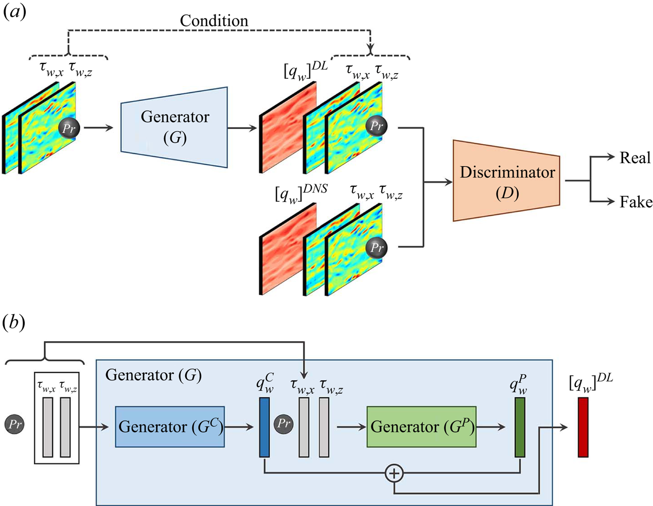
To efficiently extract the Prandtl number effect, we combined cGAN with a decomposition algorithm that decomposes turbulence data to separate the Prandtl number effect feature from a common feature. As shown in figure 1(a), cGAN with a decomposition algorithm consists of a generator ( $G$) and a discriminator ( $D$). To decompose the turbulence data, as shown in figure 1(b), the generator ( $G$) is divided into two parts: a parameter-independent generator ( $G^{C}$) and a parameter-effect generator ( $G^P$). First, the parameter-independent generator ( $G^{C}$) extracts $Pr$-independent features that contain common characteristics in turbulent data regardless of the physical parameters. The parameter-effect generator ( $G^{P}$) extracts features that are characteristic of the physical parameters. We applied this model to predict and interpret the surface heat flux using the physical parameter $Pr$. During training, the parameter-independent generator ( $G^{C}$) uses the wall-shear stresses as input data to generate a $Pr$-independent or common feature ( $q_{w}^{C}$) of the surface heat flux observed for all $Pr$. The parameter-effect generator ( $G^{P}$) predicts the Prandtl number effects ( $Pr$-dependent) feature of the surface heat flux, $q_{w}^{P}$, using the wall-shear stresses, $Pr$-independent features and $Pr$ as input data. The surface heat flux ( $q_{w}=q_{w}^{C}+q_{w}^{P}$) is the sum of the $Pr$-independent and $Pr$-dependent features. The $Pr$-independent feature obtained through this algorithm is valid for the range of Prandtl numbers in the training data used in the learning process. The discriminator ( $D$) uses the surface heat flux, wall-shear stresses and $Pr$ as input data, where the wall-shear stresses and $Pr$ are the constraints for the discriminator ( $D$). In other words, the input data of the discriminator ( $D$) consists of four components: the surface heat flux, streamwise and spanwise wall-shear stresses, and $Pr$. The loss function used for training was
 \begin{equation} \mathcal{L}_{total}=\mathcal{L}_{cGAN} + \lambda_{1} \mathcal{L}_{mse} + \lambda_{2} \mathcal{L}_{Pr}, \end{equation}
with
 $$\begin{gather} \mathcal{L}_{mse} = \mathbb{E}\left[\frac{1}{N_{p}}\| G(x,Pr) - y\|_{2}^{2}\right], \end{gather}$$
 $$\begin{gather}\mathcal{L}_{Pr} = \mathbb{E}\left[\frac{1}{N_{p}}\|G^{P}(x,G^{C}(x), Pr)\|_{2}^{2}\right], \end{gather}$$
where the total loss function consists of three losses in (2.5). Here  $\lambda _{1}$ and $\lambda _{2}$ are fixed at 200 and 10, respectively. The first and second terms on the right-hand side are the cGAN loss and mean squared loss (MSE), respectively. The last term is the physical parameter loss, which allows the surface heat flux to decompose the $Pr$-independent and $Pr$-dependent features. Through the physical parameter loss, the common characteristics of the surface heat flux were extracted to the maximum, and the features for the effect of $Pr$ were extracted to the minimum. In (2.6), $N_p$ is the number of grid points of input and output; $x$ and $y$ are the wall-shear stress and the surface heat flux from DNS, respectively, and $G(x)$ denotes the surface heat flux predicted by the generator. In (2.7), $G^{P}(x)$ is a $Pr$-dependent feature generated by the parameter-effect generator; $G^{C}(x)$ is the $Pr$-independent feature generated by the parameter-independent generator. In (2.5) the parameters of the generator ( $G$), including $G^{C}$ and $G^{P}$, are trained in the direction of minimizing $\mathcal {L}_{total}$, and the parameters of the discriminator ( $D$) are trained in the direction of maximizing $\mathcal {L}_{cGAN}$. Through training based on our designed loss function, the decomposed features are almost deterministic regardless of the model structure, but tuning of the weight coefficient of the loss is required. Thus, we present an alternative two-step learning method that can eliminate the hyperparameter. In the first step, the distance between the $Pr$-independent feature $G^C(x)$ obtained from input $x$ and the target $y$ is minimized and the trainable parameters only in $G^C$ are trained here. In the second step, the distance between the total heat flux $G(x)$ and the target $y$ is minimized and the trainable parameters in $G$ except for $G^C$ are trained. Through this process, the decomposed features can be extracted without tuning of such a hyperparameter, although we prefer to use non-separated one-step learning.
Architecture of cGAN with a decomposition algorithm. (a) Overview of cGAN consisting of generator ( $G$) and discriminator ( $D$). (b) Generator (G) including parameter-independent generator ( $G^C$) and parameter-effect generator ( $G^P$).
The cGAN loss function defined above has the problem of divergence because the discriminator can distinguish between the fake image (generated image) and the real image before the generator is sufficiently trained. In addition, after training, the generator has a mode-collapse problem, in which the generator produces only limited images. For stable training of cGAN, we used Wasserstein GAN (WGAN)-GP loss with an added gradient penalty (Gulrajani et al. Reference Gulrajani, Ahmed, Arjovsky, Dumoulin and Courville2017). The WGAN-GP enables stable learning and performance improvement by continuously generating a probabilistic divergence between the distribution of the real image and that of the generated image with respect to the parameters of the generator.
The generator ( $G$) and discriminator ( $D$) of cGAN employ a CNN, which consists of convolution operations and a nonlinear function that can effectively extract spatial patterns. Additionally, a skip connection is applied to the generator ( $G$) to effectively handle the information for large-scale structures and the trainable parameters. The generator ( $G$) makes use of downsampling and upsampling operations. Downsampling was applied to the discriminator ( $D$), however, its last two layers were fully connected. The nonlinear function used in the network was a leaky rectified linear unit (leaky ReLU), which is commonly applied to GAN-based models,
 \begin{equation} f(x) =max( \alpha x, x) ,\end{equation}
where  $\alpha$ is fixed at 0.2. This function prevents the differential value from becoming $0$ when $x<0$ so that the weights can be updated stably. Appendix A provides a detailed description of the network.
To evaluate the prediction accuracy of cGAN, we additionally considered a multiple-linear model, a shallow CNN and a CNN model as comparative models in § 3.1. The multiple-linear model and CNN have the same architecture as the generator ( $G$) of cGAN, and use the same input information size. The shallow CNN called ShallowCNN consists of two convolution layers with the 16 hidden feature maps without the decomposition algorithm, and uses less input information on a $5\times 5$ stencil than other models. The multiple-linear model used a linear function rather than a nonlinear function. For training the comparative models, the loss function to minimize is defined as
 \begin{equation} \mathcal{L}= \lambda_{1} \mathcal{L}_{mse} + \lambda_{2} \mathcal{L}_{Pr} + \lambda_{3} \sum_{i} \frac{1}{2}w_i^2 , \end{equation}
where the first and second terms on the right-hand side are the mean squared error and the physical parameter loss, respectively. The last term implies an L2 regularization to prevent overfitting and  $w_i$ are the weights; $\lambda _{1}, \lambda _2$ and $\lambda _{3}$ are 1, 0.05 and 0.0001, respectively. The loss function of ShallowCNN consists only of the mean squared error and L2 regularization, unlike those of the multiple-linear model and CNN. Appendix A provides a detailed description of the architecture such as the number of layers and feature maps for cGAN and comparative models, CNN and multiple-linear model.
3. Results and discussion
3.1. Prediction of surface turbulent heat flux
In this section we present the results of the cGAN with a decomposition algorithm for predicting the surface heat flux  $q_w$ from the streamwise and spanwise wall-shear stresses $\tau _{w,x}$ and $\tau _{w,z}$ in a turbulent channel flow. Before training our model, we investigated the fundamental behaviour of the surface heat flux and its relationship to the wall-shear stresses for the range of $Pr$ considered in this study using DNS data. Basic statistics such as the Nusselt number ( $Nu=2\delta h/k=2\langle q_w \rangle$; where $h$ and $k$ are the heat transfer coefficient and thermal conductivity of fluid, respectively, and $\langle \rangle$ denotes an average operation), and r.m.s. of fluctuations $q_{w,rms}$ are presented in figure 2. The Nusselt number shows two distinct limiting behaviours, as shown in figure 2(a): it increases monotonically with $Pr$ for $Pr \geq 0.1$, while it converges to $1$ with decreasing $Pr$, indicating that the temperature field approaches a linear profile, which is a signature of pure conduction heat transfer across the channel. As $Pr$ decreases, the r.m.s. value of the surface heat flux decreases, as shown in figure 2(b), as $q_{w,rms}/\langle q_w \rangle \simeq 10.67 Pr$. The distribution becomes Gaussian, as shown in figure 24 in Appendix C. However, the r.m.s. value remained at 40 % of the mean value as $Pr$ increased.
Statistics obtained from DNS data. (a) Relation between Prandtl numbers and Nusselt numbers. (b) Root mean square of surface heat flux with  $Pr$.
$Pr$.

The correlation between the surface heat flux and wall-shear stress is presented in figure 3 in terms of the correlation coefficient  $R(\equiv \langle \tau '_w q'_w\rangle / (\sigma (\tau _w) \sigma (q_w)) )$ and the scatter plot. Here, $\tau _{w}$ = $\sqrt {\tau _{w,x}^2+\tau _{w,z}^2}$, and superscript $'$ and $\sigma$ denote the fluctuation and standard deviation, respectively. The correlation coefficient shows a peak greater than 0.9 at $Pr =1$, and a strong correlation is seen in the scatter plot. These clearly support the Reynolds analogy. For the range $0.1 \leq Pr \leq 10$, a certain level of correlation is observable, whereas for $Pr < 0.1$, the two quantities are hardly correlated, although the correlation coefficient approaches the limiting value of 0.2, as $Pr$ approaches zero. These observations indicate that as $Pr$ approaches 0, the surface heat flux is mostly determined by the conduction process, and convection due to turbulence has little effect. Therefore, we focus on the range of $Pr=0.1\unicode{x2013}7$ and present the results for this range in the main text. The training and prediction results for $Pr=0.001\unicode{x2013}0.05$ are presented in Appendix C.
Relation between wall-shear stresses and surface heat flux for the Prandtl number obtained from DNS data. (a) Correlation coefficient. (b) Scatter plots.

The network was trained for  $Pr = 0.2, 0.71, 2$ and $5$, and the trained network was tested for $Pr = 0.1, 0.2, 0.4, 0.71, 1, 2, 3, 5$ and $7$. As shown in figure 2, for the range of $Pr$ considered here, the mean surface heat flux exhibits two slightly different scaling behaviours in $Pr$ depending on whether $Pr$ is less than or greater than one, whereas the r.m.s. value shows almost the same behaviour as the mean value. When the surface heat flux fields for various $Pr$ were used together as the output in training, the training sometimes became unstable due to the different ranges of output fields. To alleviate this problem, the surface heat flux fields were normalized using empirical scaling between $Nu$ and $Pr$. Ignoring the difference between the two scaling relations in figure 2(a), we used the heat flux fields normalized by $Pr^{1/2}$, the empirical correlation indicating that the Nusselt number is a function of the Prandtl number, as the output. The wall-shear stresses and input data were normalized to have $\text {mean}=0$ and $\text {std}=1$. The training and validation data were 1000 and 100 in number, respectively, with $\Delta t^+=9$, which is an interval of data fields, for trained $Pr$; and the number of testing data was 1000 with $\Delta t^+=9$ for all $Pr$. The superscript ( $+$) indicates that these parameters were normalized by $u_\tau$ and $\nu$ and made dimensionless. The testing data were sufficiently decorrelated from the training data. In the training process, a randomly sampled subregion ( $64 \times 64$) in the $x$-
$x$- $z$ plane was used for the input and output data. The subregion is of a sufficiently large size, over which the correlation decays to almost zero in two-dimensional two-point correlation between the wall-shear stresses and surface heat flux for all $Pr$. Furthermore, we double checked through an analysis of the trained model that the input information in a much smaller region than the subregion is mainly used for prediction. Before presenting the prediction results, we want to emphasize that our model does not overfit the training data based on the comparison of the training and validation errors of cGAN, presented in Appendix B.
To provide an idea of the structures in the surface heat flux for various Prandtl numbers, the surface heat flux fields for  $Pr$ predicted for the same wall-shear stresses using cGAN in a domain smaller than the full domain are shown in figure 4. The wall-shear stresses and predicted $q_w$ values are presented in figures 4(a) and 4(b), respectively. The surface heat flux field for $Pr=0.71$ was very similar to the streamwise wall-shear stress, and a high local heat flux was observed at the location where the wall-shear stress was strong. When $Pr=0.1$, the surface heat flux distribution was smoother in the spanwise direction and wavier in the streamwise direction than that for $Pr=0.71$, whereas the thermal structures for $Pr=2$ were elongated in the streamwise direction and sharper in the spanwise direction than in the case of $Pr=0.71$. This trend strengthens as $Pr$ increases. Small-scale structures appeared in the predicted fields for $Pr=7$. In other words, the thermal structures tend to become streakier as $Pr$ increases.
Surface heat flux fields for various  $Pr$ obtained from same input data using cGAN. (a) Streamwise and spanwise wall-shear stress used as input data. (b) Surface heat flux with $Pr$.
$Pr$.

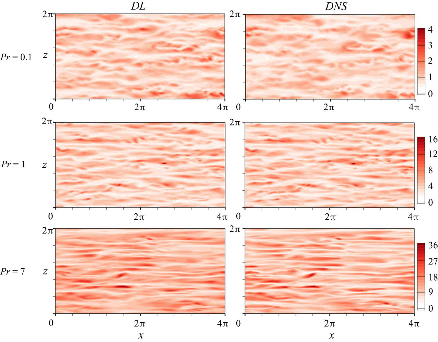
For the qualitative evaluation of the performance of the developed network, instantaneous surface heat flux fields in the whole domain predicted by cGAN compared with DNS data for trained Prandtl and untrained Prandtl numbers are shown in figures 5 and 6, respectively. As shown in figure 5, cGAN slightly underpredicted the local maximum values of  $q_w$ for $Pr=0.2$ observed in DNS, whereas the predicted surface heat flux shows an overall similar distribution to that of DNS by capturing small-scale variations. In contrast, our model can generate streaky structures observed in $q_w$ for $Pr=0.71$ and $5$. As shown in figure 6 for the untrained Prandtl numbers, our model slightly overpredicts the surface heat flux field compared with DNS for $Pr=0.1$. The predicted surface heat flux fields for $Pr=1$ and $7$ were consistent with those of DNS. Therefore, we confirmed that our model could generate surface heat fluxes similar to those of DNS for untrained $Pr$ and trained $Pr$.
$Pr$.
Instantaneous surface heat flux for trained  $Pr$ obtained from wall-shear stresses using cGAN.

Instantaneous surface heat flux for untrained  $Pr$ obtained from wall-shear stresses using cGAN.
To quantitatively assess the prediction accuracy of cGAN, we additionally considered CNN, ShallowCNN and multiple-linear models as comparative models. In table 2 we provide the correlation coefficient  $R$ between surface heat flux of DNS data and that predicted by DL models, where $R ={\langle q^{'DNS}_{w} q^{'DL}_{w}\rangle / ({\sigma (q^{DNS}_{w})}{\sigma (q^{DL}_{w})}})$, demonstrating that CNN has a higher correlation coefficient for all untrained $Pr$ than those obtained from the linear model and cGAN. The correlation coefficient $R$ for cGAN is slightly lower than that for CNN, whereas ShallowCNN and the linear model have a relatively low correlation coefficient, particularly for $Pr = 0.2$ and 5. ShallowCNN predicts heat flux better than linear models, but not as accurate as CNN with more layers. This indicates that there is a complex nonlinear relation between the local heat flux and the wall-shear stresses, suggesting that a sufficiently large number of layers should be used to develop an integrated model for $Pr$. For the untrained $Pr$, the performance of all models is similar to that of the trained $Pr$. Commonly, the performance of all models is best for $Pr$ around 1, and the performance deteriorates as $Pr$ increases or decreases because the temperature is not dominantly determined by the near-wall transport and the dissimilarity becomes very strong. Furthermore, the slight inaccuracy might be caused by an improper normalization technique, which is needed for learning data of highly different scales. However, the prediction by CNN and cGAN is good for the tested range. Because CNN learns to minimize the pointwise error between DNS data and generated data, the correlation coefficient of CNN is naturally higher than that of cGAN. One might think that CNN is better than the GAN-based model by comparing the point-by-point error, but CNN is somewhat inaccurate in the prediction of statistics, as shown below. To improve the prediction performance of the model, we considered a cGAN model using wall pressure fluctuations and wall-shear stresses as input information. The predictive performance of the model was improved when additional pressure fluctuations were used, but only marginally, as shown in table 4 in Appendix D, where the performance of the model with pressure data as input is provided in detail. The pressure information was found to be auxiliary in the prediction of the surface heat flux. Consequently, only the wall-shear stresses were considered as input information.
Correlation coefficient between target data (DNS data) and surface heat flux for trained and untrained  $Pr$ predicted by various learning models.

To investigate the performance of the models in more detail, we present the basic statistics of the surface heat flux, such as the Nusselt number, r.m.s., skewness and flatness in figure 7. Because the heat flux is normalized by  $Pr^{1/2}$ based on our observation, which is not accurate, the predicted mean such as the Nusselt number needs to be checked. As shown in figures 7(a) and 7(b), the Nusselt number and r.m.s. predicted by cGAN and CNN are very accurate compared with those by DNS for both trained and untrained $Pr$. On the other hand, the multiple-linear model predicts the Nusselt number relatively well because of the use of empirical correlation but underpredicts the r.m.s. values. As shown in figures 7(c) and 7(d), cGAN produces the smallest errors for all $Pr$, whereas the CNN and multiple-linear models underpredict the skewness and flatness factors for all $Pr$. These results confirm that the multiple-linear model is not suitable for prediction in the considered range of $Pr$.
$Pr$.
Statistics of surface heat flux for trained  $Pr$ (0.2, 0.71, 2, 5) and untrained $Pr$ (0.1, 0.4, 1, 3, 7) obtained using DL models; (a) $Nu$, (b) r.m.s., (c) skewness, (d) flatness.
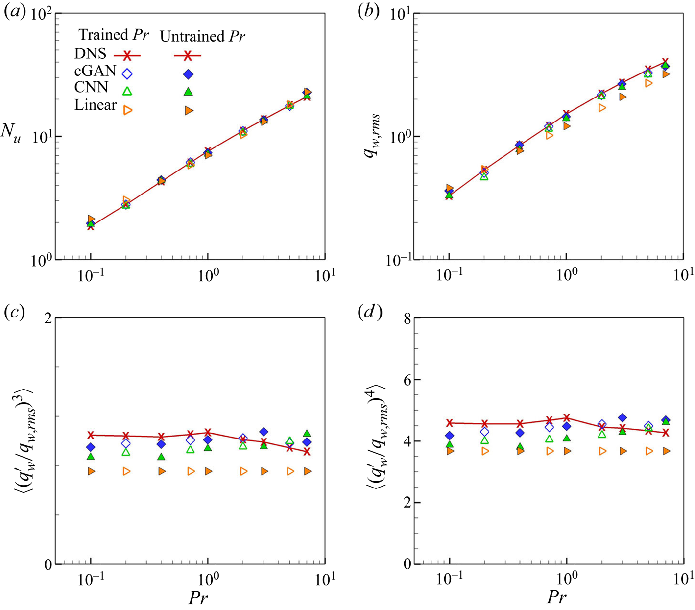
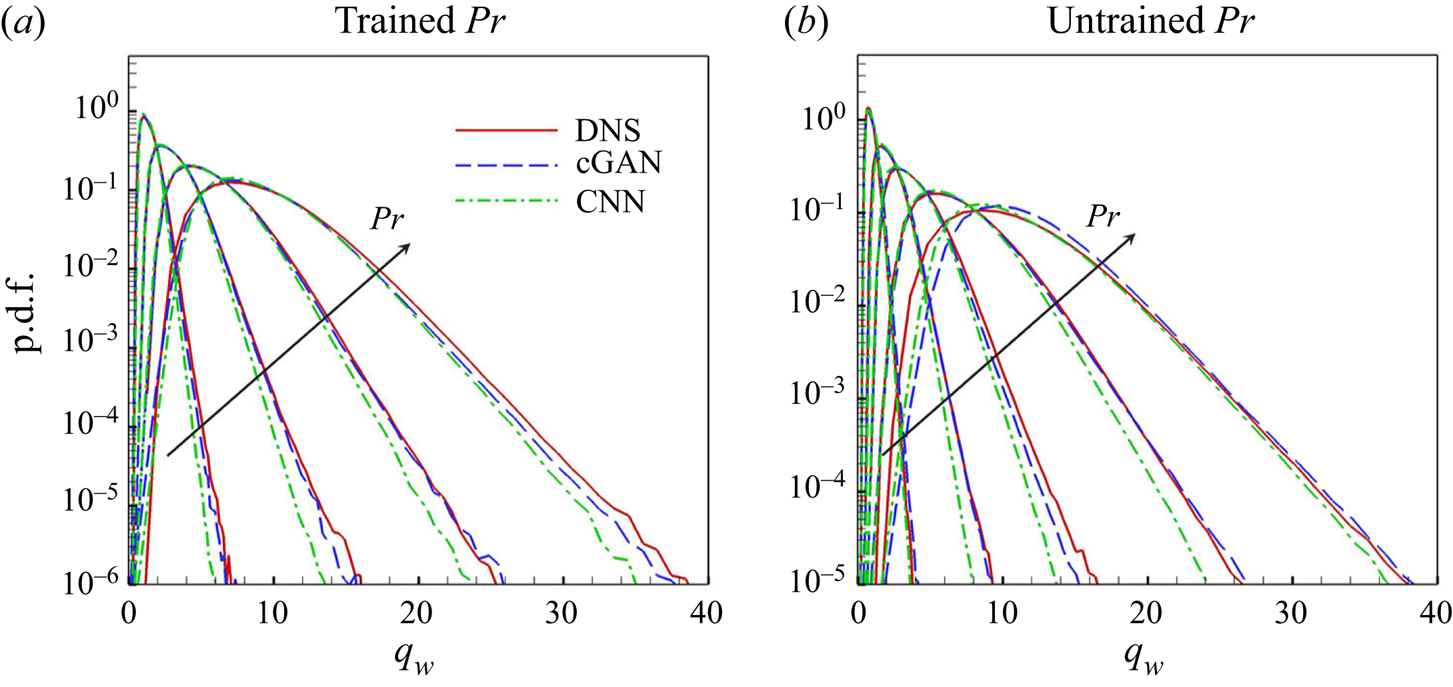
Figure 8 compares the probability distribution function (PDF) of the surface heat flux predicted for the trained and untrained  $Pr$ with the DNS data. In this investigation only the results of the cGAN and CNN are presented, except for the multiple-linear model, which showed the lowest accuracy of the previous statistics. As shown in figure 8(a), both cGAN and CNN produce a PDF for the trained $Pr$ that is similar to that of DNS, but cGAN outperforms CNN in capturing high values of the surface heat flux for the trained $Pr$. For the untrained $Pr$, the prediction performance of the two models is comparable to that of the trained $Pr$, as shown in figure 8(b); however, cGAN outperforms CNN. Given that this type of statistical information is not used in training, our model captures the asymmetric statistical nature remarkably well. As $Pr$ decreases, the PDF tends to recover symmetry, gradually becoming a Gaussian distribution, as shown in figure 24 in Appendix C.
Probability density function (p.d.f.) of surface heat flux for (a) trained  $Pr$ ( $=0.2, 0.71, 2, 5$) and (b) untrained $Pr$ ( $=0.1,0.4,1,3,7$) obtained through DL models. Arrows indicate increasing $Pr$.
$Pr$.
Additionally, we examined the energy spectrum of the surface heat flux for the reproducibility of scale behaviour. The streamwise and spanwise energy spectra of  $q_w$ are defined as
 \begin{equation} E(\kappa_x) = \frac{1}{{2{\rm \pi}}}\int_{-\infty}^{\infty}\,{{\rm e}^{-{\rm i}p\kappa_x}\phi(p)\, {\rm d} p},\quad E(\kappa_z) = \frac{1}{2{\rm \pi}}\int_{-\infty}^{\infty}\,{\rm e}^{-{\rm i}q\kappa_z}\psi(q)\, {\rm d} q, \end{equation}
with
 \begin{equation} \phi(p) = \langle q'_w(x,z)q'_w(x+p,z)\rangle ,\quad \psi(q) = \langle q'_w(x,z)q'_w(x,z+q)\rangle ,\end{equation}
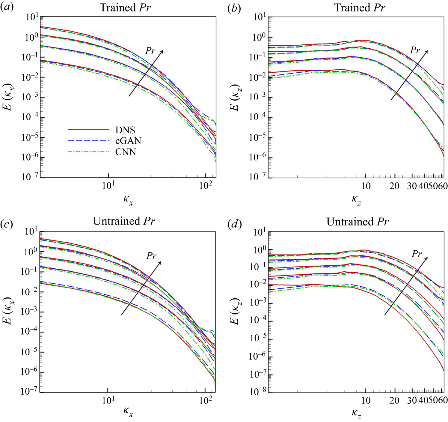
where  $\phi (p)$ and $\psi (q)$ are the two-point correlations of the surface heat flux in the $x$ and $z$ directions, respectively. As shown in figures 9(a) and 9(b) for the trained $Pr$, cGAN produces a spectrum that matches well with that obtained from DNS for all ranges of both wavenumbers, whereas CNN underestimates the streamwise spectrum for all wavenumbers and the spanwise spectrum for low wavenumbers. For the untrained $Pr$, the performance of cGAN does not deteriorate in the prediction of the streamwise spectrum, except for $Pr=0.1$, whereas CNN tends to underestimate the spectrum except for $Pr=0.1$, which appears to be coincidental, as shown in figure 9(c). However, the prediction of the spanwise spectrum by both cGAN and CNN worsens, especially for high wavenumbers, as shown in figure 9(d). It is noteworthy that both cGAN and CNN do not perform well for $Pr=0.1$, because as $Pr$ decreases, the surface heat flux becomes less dependent on the wall-shear stresses, as discussed in Appendix C. Overall, cGAN shows better performance in capturing statistical characteristics than CNN because statistical consistency is considered in the training process of the cGAN through the discriminator network, in addition to the local loss based on pointwise errors.
One-dimensional energy spectra of surface heat flux for various  $Pr$ obtained from wall-shear stresses through DL models. Arrows indicate increasing $Pr$. (a) Streamwise and (b) spanwise energy spectrum of surface heat flux with trained $Pr(=0.2, 0.71, 2, 5)$; (c) streamwise and (d) spanwise energy spectrum of surface heat flux with untrained $Pr(=0.1,0.4,1,3,7)$.
In order to provide a reliable interpretation of the trained model, which will be discussed in §§ 3.2 and 3.3, we investigated whether the model well reflects the spatial correlation between the wall-shear stresses and the surface heat flux. The two-dimensional two-point correlation between the surface heat flux at a point  $(x,z)$ and the wall-shear stresses at a point $(x+r_x,z+r_z)$ is defined by
 \begin{equation} R_{V_{1} V_{2}}(r_{x},r_{z})= \frac{\langle V'_{1}(x,z)V'_{2}(x+r_{x},z+r_{z})\rangle}{\sigma(V_{1}) \sigma(V_{2})}, \end{equation}
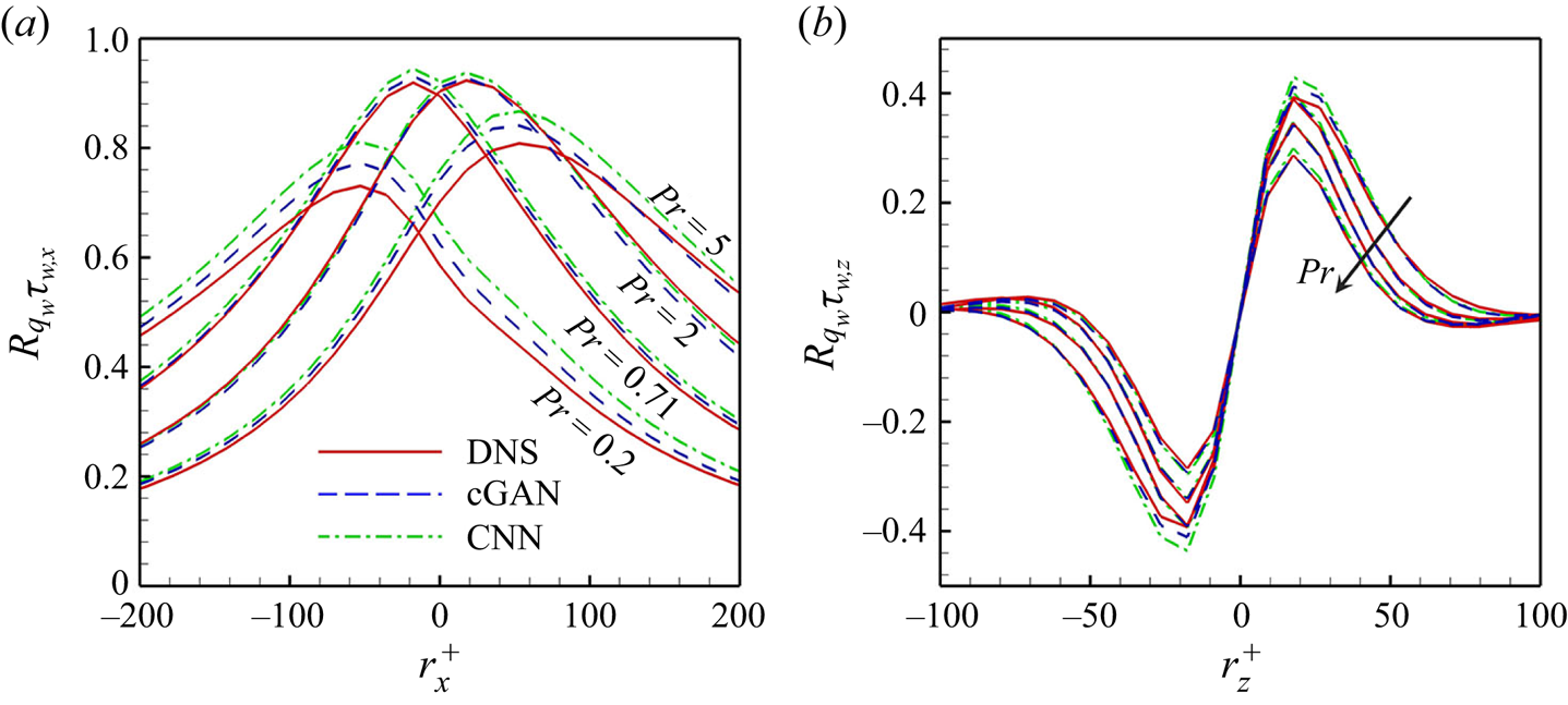
where  $V_{1}$ and $V_{2}$ represent $\tilde {q}_{w}$ and $\tilde {\tau }_{w}$, respectively. The two-point correlation between the wall-shear stresses and surface heat flux predicted through cGAN and CNN for the trained $Pr$ is presented in figure 10. In $R_{q_{w}\tau _{w,x}}(r_x,0)$, both cGAN and CNN well reflect the spatial shifting phenomenon of the correlation peak location depending on the Prandtl number, which is observed in DNS (figure 10a). However, for $Pr = 0.2$ and $5$, CNN highly overestimates the maximum values of DNS, whereas cGAN reproduces the correlation more accurately than CNN. These results indicate that cGAN, unlike CNN, generates a more input-dependent output by using input information as conditions in the learning process. Figure 10(b) shows $R_{q_{w}\tau _{w,z}}(r_{x,max}, r_z)$, where the streamwise location $r_{x,max}$ is the maximum location of $R_{q_{w}\tau _{w,z}}$ for each $Pr$. The cGAN and CNN follow DNS well overall, while cGAN presents slightly better correlation for the lowest $Pr$. In addition, the models reflected well the symmetric properties and the decorrelated tendency with an increase in $Pr$. Although the models present a relatively inaccurate two-point correlation for untrained $Pr$ (not shown here), it is obvious that cGAN predicts the spatial correlation between input and target better than CNN. Therefore, it seems reasonable to focus on the interpretation of cGAN rather than CNN.
Two-point correlations (a)  $R_{q_{w}\tau _{w,x}}(r_x,0)$ along the streamwise direction and (b) $R_{q_{w}\tau _{w,z}}(r_{x,max}, r_z)$ along the streamwise direction for trained $Pr(=0.2,0.71,2,5)$.
From all the tests in this section, we confirm that cGAN is able to predict the surface heat flux for various  $Pr$ values using only the wall-shear stress information. In addition to the prediction of pointwise distribution of the surface heat flux, cGAN captures statistical features very well compared with DNS for the trained $Pr$. Meanwhile, for the untrained $Pr$, our model showed the highest accuracy among other models, including CNN and multiple-linear models, exhibiting an accuracy comparable to that of the trained $Pr$. These results indicate that our model can distinguish the effect of the Prandtl number well and can express the relationship between the wall-shear stresses and the surface heat flux depending on $Pr$. The performance of CNN and cGAN is not extremely different in this application, but in a situation where the input information is insufficient, CNN can generate an output with non-physical characteristics and highly underestimate the target magnitude. On the other hand, a GAN-based network can generate an output that reflects physical or statistical properties of turbulence, although the pointwise error is slightly higher than CNN (Ledig et al. Reference Ledig2016; Deng et al. Reference Deng, He, Liu and Kim2019; Lee & You Reference Lee and You2019; Kim et al. Reference Kim, Kim, Won and Lee2021). It is highly probable that a GAN-based network tries to find a solution in the space that satisfies physical and statistical properties of turbulence data. Therefore, GAN is considered as a promising tool for the generation and modelling as well as prediction of turbulence. In addition, although we tested the Prandtl number effect only, we expect that our model could work well for a higher Reynolds number from previous studies (Kim & Lee Reference Kim and Lee2020b; Kim et al. Reference Kim, Kim, Won and Lee2021), where the DL model showed successful predictions for a higher Reynolds number than the trained number under the condition that grid resolution of input is the same as that of the trained one and input data are normalized by proper length and velocity scales (e.g. the viscous length scale and friction velocity in wall turbulence).
3.2. Interpretation of DL model
By observing the gradient maps obtained from the trained DL model, we attempt to analyse the physical relationship between the input and output of our prediction network. For the analysis, a cGAN was used, which is the most accurate model as discussed in § 3.1. We only investigated the surface heat flux for the trained  $Pr$. Because the mean surface heat flux is very different for different Prandtl numbers, it is difficult to accurately analyse their effect. For the reliability of the analysis, cGAN was trained using data preprocessed by different methods. The surface heat flux for each $Pr$ was normalized so that its $\text {mean}=1$, and the normalized value is denoted by $\tilde {q}_{w}$. The wall-shear stresses were normalized to have $\text {mean}=0$ and $\text {std}=1$, and the normalized stress is denoted by $\tilde {\tau }_{w}$. Furthermore, we performed data augmentation by applying spanwise symmetry and a phase shift, considering the characteristics of the channel flow and boundary conditions.
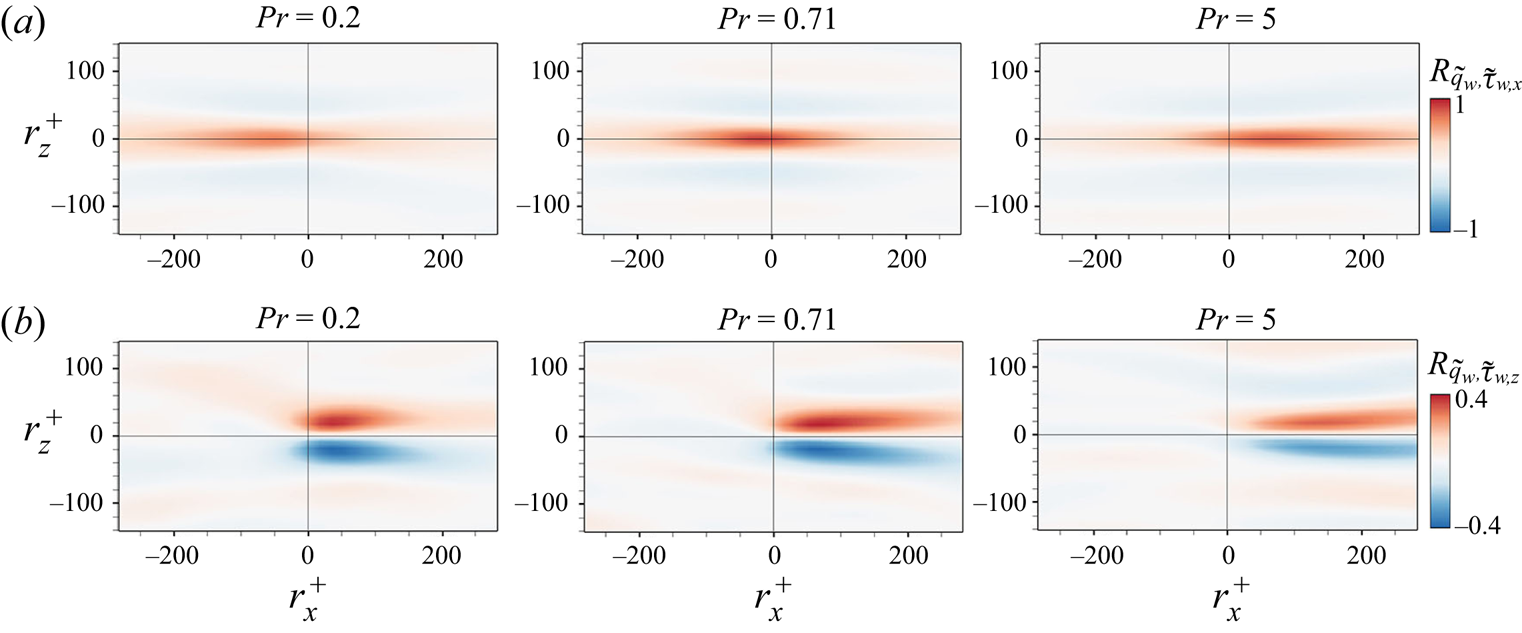
Prior to interpreting the physical relationship between the surface heat flux and wall-shear stresses based on the gradient maps, we observed two-dimensional two-point correlation  $R_{\tilde {q}_{w}\tilde {\tau }_{w}}$ for $Pr=0.2, 0.71$ and $5$ obtained from DNS data in figure 11, which is calculated by (3.3). As shown in figure 11(a), the peak correlation of the streamwise shear stress for $Pr=0.2$ and $0.71$ is observed in the upstream region at approximately $r_x^+=-60$, $r_z^+ \simeq 0$ and $r_x^+=-10, r_z^+\simeq 0$, respectively, whereas that for $Pr=5$ is found approximately at $r_x^+=80, r_z^+\simeq 0$. This shift in the location showing peak correlation can be understood using the convection velocity of temperature near the wall; the convection velocity of temperature for $Pr < 1$ is higher than that of the streamwise velocity and vice versa for $Pr >1$ (Kowalewski, Mosyak & Hetsroni Reference Kowalewski, Mosyak and Hetsroni2003; Abe et al. Reference Abe, Kawamura and Matsuo2004). Depending on $Pr$, the dominance of thermal diffusion and momentum diffusion enhances the convection velocity. Similar to the effect of the Prandtl number, it has been reported that the local concentration field response to velocity fluctuations in turbulent mass transfer has a significant time lag for high Schmidt numbers (Shaw & Hanratty Reference Shaw and Hanratty1977; Hasegawa & Kasagi Reference Hasegawa and Kasagi2009), explaining the spatial shifting phenomenon of surface heat flux well. On the other hand, for all $Pr$, the correlation between the surface heat flux and the spanwise shear stress shown in figure 11(b) exhibits positive and negative correlations in the first quadrant ( $r_x^+>0$, $r_z^+>0$) and the fourth quadrant ( $r_x^+>0$, $r_z^+<0$), respectively. As $Pr$ increased, the correlation peak gradually moved in the downstream direction. This is consistent with a previous observation that the maximum correlation between the spanwise shear stress and streamwise vortices near the wall occurs downstream (Kravchenko, Choi & Moin Reference Kravchenko, Choi and Moin1993). In addition, as $Pr$ increases, the correlation weakens, and its distribution is stretched in the streamwise direction.
Two-dimensional two-point correlation of (a) streamwise wall-shear stress ( $\tilde {\tau }_{w,x}$) and (b) spanwise wall-shear stress ( $\tilde {\tau }_{w,z}$) with respect to surface heat flux ( $\tilde {q}_{w}$) for $Pr$ obtained from DNS data.
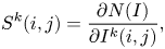
A two-point correlation between two variables indicates that there exists a relationship between them, but it does not reveal any information about the cause-and-effect relationship between them. To investigate the cause-and-effect relationship between the wall-shear stresses and surface heat flux, we performed a sensitivity analysis between the input and output of the trained DL model. Sensitivity analysis has been applied to image classification and regression problems, which enables the analysis of the relationship between the input and output (Simonyan, Vedaldi & Zisserman Reference Simonyan, Vedaldi and Zisserman2013; Kim & Lee Reference Kim and Lee2020b). From a sensitivity analysis, we can determine the reasons for the inaccuracy of the DL model, which can help improve its performance. In addition, in the case of a regression problem, sensitivity analysis can provide a guide on the input size, by taking into account the essential components required for efficient training of the DL. Sensitivity analysis was performed using the gradient of the output with respect to the input as
 \begin{equation} S^k (i,j) = \frac{\partial N(I) }{\partial I^k (i,j)},\end{equation}
where  $S^k(i,j)$ is the gradient map of the input variables ( $k$), such as the wall-shear stresses at $(x+r_x, z+r_z)$, with $r_x=i\Delta x$ and $r_z=j\Delta z$. Here $I^k(i,j)$ is an input variable at $(x+r_x, z+r_z)$ and $N(I)$ is an output variable, such as the surface heat flux, obtained from the output of DL at $(x,z)$; $i = -(m_{x}-1)/2 \sim (m_{x}-1)/2$ and $j = -(m_{z}-1)/2 \sim (m_{z}-1)/2$, where $m_x \times m_z$ is the input kernel size. The gradient map indicates the sensitivity of the change in the surface heat flux at a point with respect to the change in the wall-shear stress around that point. Due to the nonlinearity of the trained model, the gradient map typically varies with the spatial location of the predicted heat flux, unlike a linear model that applies the same operation regardless of spatial location (Kim & Lee Reference Kim and Lee2020b). Therefore, the significant difference between a DL model and a linear model could be understood by the input-dependent nature observed in the gradient map.
Through an investigation of the gradient map, we were able to analyse how the wall-shear stresses affected the surface heat flux. However, the recognition of meaningful patterns in the gradient map is not straightforward because of the noise generated in the complicated learning process of the non-unique relationship between the input and output. Therefore, we first investigated an average gradient map  $\bar {S}^{k}$ (where $\bar {{\cdot }}$ is the average operation in space and time), which is an average of the instantaneous gradient maps of input variables $(k)$ obtained at various locations of output in space over a time span.
The average gradient maps  $\bar {S}^{\tilde {\tau }_{w,x}}$ and $\bar {S}^{\tilde {\tau }_{w,z}}$ for the local heat flux $\tilde {q}_w$ with respect to the streamwise wall-shear stress $\tilde {\tau }_{w,x}$ and spanwise wall-shear stress $\tilde {\tau }_{w,z}$ for various $Pr$ are presented in figures 12(a) and 12(b), respectively. As shown in figure 12(a), non-trivial values of $\bar {S}^{\tilde {\tau }_{w,x}}$ are observed in a local region of the input fields for all $Pr$, indicating that DL primarily uses the local information of the input field $\tilde {\tau }_{w,x}$ to predict the heat flux at a point. The magnitude of the gradient is small for $Pr=0.2$ compared with the cases for $Pr=0.71$ and $5$, implying that the surface heat flux at $Pr=0.2$ is relatively less sensitive to the change in $\tilde {\tau }_{w,x}$ than that at $Pr=0.71$ and $5$. An important characteristic observed in $\bar {S}^{\tilde {\tau }_{w,x}}$ is that a positive peak is found in the upstream region for $Pr < 1$, whereas in the downstream region the peak is found for $Pr > 1$. The peaks for $Pr=0.2, 0.71$ and $5$ occur at $r_x^+=-20, 0$ and $30$, respectively. Although the specific peak locations are different, this behaviour is similar to that of the two-point correlation shown in figure 11(a). The shift of a peak observed in the gradient maps presents an important observation that the DL model predicts local heat flux by reflecting the physical features affected by large-scale motion as the Prandtl number decreases. Also, the fact that the region showing high two-point correlation for all $Pr$ is much longer in the streamwise direction than the region with a non-trivial gradient map indicates that the average gradient map pinpoints the region of input that influences the output on average.
Average gradient maps of surface heat flux ( $\tilde {q}_{w}$) with respect to (a) streamwise wall-shear stress ( $\tilde {\tau }_{w,x}$) and (b) spanwise wall-shear stress ( $\tilde {\tau }_{w,z}$) for $Pr$ obtained through cGAN. The average gradient maps were obtained using a sufficiently large amount of instantaneous gradient maps, where the number of data are $81\ 920$ (all points in five fields with $N_x=N_z=128$ and $\Delta t^+=9$) for each $Pr$.
$Pr$.
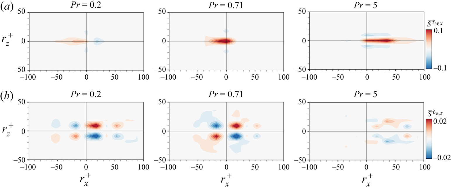
In figure 12(b) the average gradient map  $\bar {S}^{\tilde {\tau }_{w,z}}$ shows a skew-symmetric pattern in the spanwise direction $\bar {S}^{\tilde {\tau }_{w,z}}(i,j)=-\bar {S}^{\tilde {\tau }_{w,z}}(i,-j)$ for all $Pr$. For $Pr=0.2$, the gradient map was pronounced in the first and fourth quadrants, and a high sensitivity for $Pr=0.71$ was observed in all quadrants. The gradient map for $Pr=0.71$ indicates that the local heat flux can be enhanced when a pair of vortices is located downstream, or when a vortex crosses diagonally at the centre point, even when the streamwise wall-shear stress is weak (Kim & Lee Reference Kim and Lee2020b). However, the gradient for $Pr=5$ is relatively weak everywhere, implying that the surface heat flux at $Pr = 5$ is hardly influenced by the spanwise wall-shear stress compared with other Prandtl numbers. These patterns in the gradient maps, which were not observed in the two-point correlation in figure 11(b), indicate that the model can capture intermittent physical phenomena through a combination of multi-point streamwise and spanwise wall-shear stresses. We also observed the average gradient map of the model predicting the surface heat flux from the wall-shear stresses and pressure fluctuations; the results are presented in detail in Appendix D.
Next, we investigate the instantaneous gradient map for specific flow situations to discuss the cause-and-effect relationship between turbulent variables depending on the Prandtl number in detail. As described above, noise removal in an instantaneous gradient map is essential because noise makes it difficult to recognize and analyse meaningful patterns. Smilkov et al. (Reference Smilkov, Thorat, Kim, Viégas and Wattenberg2017) used Gaussian noise as a method to remove noise in the salient map for classification problems. However, in our problem this method did not show a remarkable effect in removing noise, and thus, we took advantage of symmetry properties such as reflectional equivariance and invariance with respect to the phase shift in the channel geometry. The reflectional equivariance property can be implemented using mirror data in the spanwise direction. Therefore, a gradient map was obtained by averaging the original gradient map and the mirrored gradient map of the mirrored data. Additionally, phase shift invariance can be implemented by averaging the instantaneous gradient maps of several data points with a phase shift of less than  $0.2\Delta x$, under the assumption that the turbulence structure does not significantly change over a small distance. To illustrate the effect of noise removal, we present instantaneous gradient maps ( $S^{\tilde {\tau }_{w,z}}$) before and after noise removal in figure 13, which clearly demonstrate the effect of noise removal. Compared with the original gradient map shown in figure 13(a), the noise-removed gradient map in figure 13(b) exhibits a more pronounced pattern, similar to the average gradient map. The gradient in the region far from the origin is very small. The instantaneous gradient maps presented in this study were obtained by applying the noise-removal method.
Effect of the noise-removal method for the instantaneous gradient map ( $S^{\tilde {\tau }_{w,z}}$) at $Pr=0.71$ obtained through cGAN. (a) Original gradient map and (b) gradient map applying both reflectional equivariance and phase shift method.

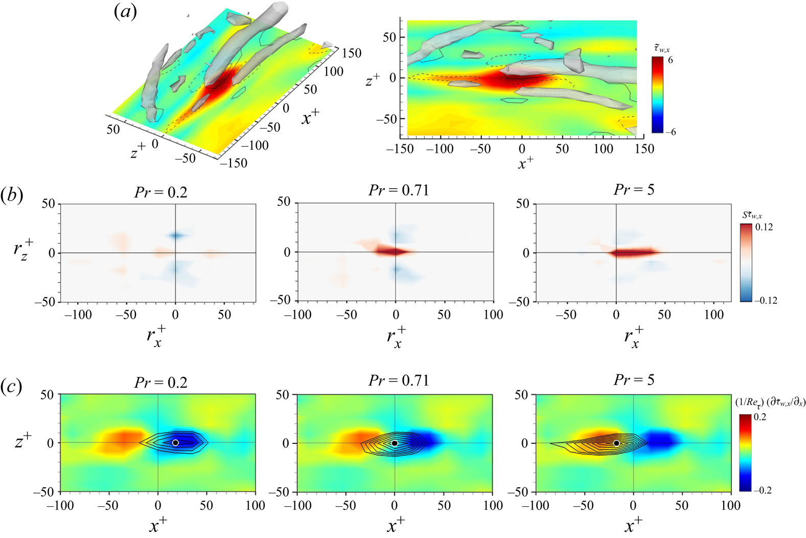
To investigate the detailed cause-and-effect mechanism based on the analysis of the average gradient map, we chose two specific examples of the flow field: one showing locally intense streamwise shear stress and the other exhibiting intense spanwise shear stress. Figure 14(a) illustrates an example with intense streamwise shear stress located at the origin. The nearby vortices are visualized using the  $\lambda _2$ method (Jeong & Hussain Reference Jeong and Hussain1995). Figure 14(b) shows instantaneous gradient maps, relative to the peak location of heat flux marked by the black dot in figure 14(c), which are similar to the average gradient maps shown in figure 12. This instantaneous gradient map suggests that the peak heat flux is caused by different parts of the nearby streamwise shear stress distribution depending on $Pr$. The peak heat flux is observed at a slightly downstream location of the peak streamwise shear stress for $Pr=0.2$, while the peak heat flux is found at a slightly upstream location of the peak stress for $Pr=5$. Because this slight shift of peaks clearly indicates that the gradient of input shear stress may play a key role in determining heat flux, we investigated the spatial gradient of input to observe the Prandtl number effect, which is also connected to sweep and ejection events by the Taylor expansion of the near-wall wall-normal velocity. The streamwise gradient of the streamwise shear stress $\partial {\tilde {\tau }_{w,x}}/\partial {x}$ shown in coloured contours in figure 14(c) clearly confirms that the negative peak of $\partial {\tilde {\tau }_{w,x}}/\partial {x}$ is observed at almost the same location as the peak heat flux for $Pr=0.2$, whereas the positive peak $\partial {\tilde {\tau }_{w,x}}/\partial {x}$ coincides with the peak heat flux location for $Pr=5$. When $Pr$ is approximately 1, the heat flux and shear stress exhibit peaks at the same location. The relatively weak sensitivity shown in the gradient map for $Pr=0.2$ in figure 14(b) is due to relatively weak heat flux in this particular situation.
Representative example of the region where dissimilarity between  $\tilde {\tau }_{w,x}$ and $\tilde {q}_{w}$ is weak and $\tilde {q}_{w}$ is high for $Pr=0.71$. (a) The right panel is the top view of the left panel. The colours and lines represent $\tilde {\tau }_{w,x}$ and $\tilde {\tau }_{w,z}$, respectively, and $\lambda _{2}^+=-0.02$. (b) The instantaneous gradient map of $\tilde {q}_{w}$ with respect to $\tilde {\tau }_{w,x}$ for $Pr$ obtained through cGAN. (c) Instantaneous contours of $\partial {\tilde {\tau }_{w,x}}/\partial {x}$ (colour) and $\tilde {q}_{w}$ for $Pr$ obtained using cGAN (lines are from 2.0 to 4.0 with increments of 0.2).
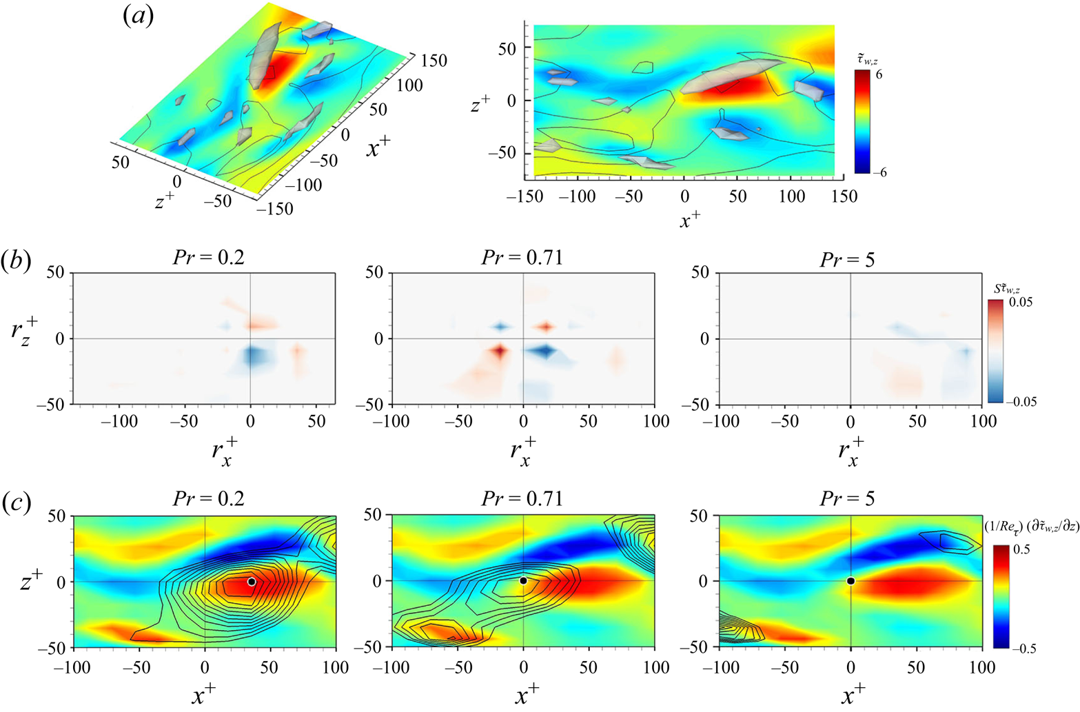
We now investigate the second example showing a strong spanwise shear stress around the peak heat flux, as demonstrated in figure 15(a). The strongest local heat flux is observed around the region with a strong positive spanwise shear stress for  $Pr=0.2$. Figure 15(b) shows the instantaneous gradient map relative to the peak heat flux location marked by the black dot in figure 15(c) for $Pr=0.2$ and 0.71. For $Pr=5$, because there is no strong heat flux observed around the black dot, the same output location as that of $Pr=0.71$ was selected in the calculation of the gradient map. The instantaneous gradient map is similar to the average gradient map of figure 12, except that the peak streamwise location of the instantaneous gradient map is almost the same as that of the heat flux, whereas the peak of the average gradient map is located slightly downstream of the heat flux. This suggests that for $Pr=0.2$, the spanwise variation of the spanwise shear stress might cause a strong local heat flux. It naturally leads to the investigation of the spanwise gradient of the spanwise shear stress (coloured contours) with the corresponding heat flux distributions (line contours) in figure 15(c). The positive spanwise gradient of the spanwise shear stress $\partial {\tilde {\tau }_{w,z}}/\partial {z}$ clearly confirms a strong correlation with the peak heat flux. On the other hand, when $Pr=5$, the strong spanwise shear stress does not contribute to the local heat flux. However, when $Pr=0.71$, the instantaneous gradient map exhibits a skew-symmetric pattern in both the streamwise and spanwise directions: $S^{\tilde {\tau }_{w,z}}(x+r_x,z+r_z)=-S^{\tilde {\tau }_{w,z}}(x+r_x,z-r_z) =-S^{\tilde {\tau }_{w,z}}(x-r_x,z+r_z)$. The only situation allowing the local heat flux at $(x,z)$ to be caused by the nearby spanwise shear stress through such a skew-symmetric sensitivity map is that a streamwise vortex is slightly slanted from the streamwise direction, as shown in figure 15(a). In the two-point correlation (figure 11) it is difficult to identify which part is necessary for prediction because correlation exists in a wide region, indicating the limitation of the conventional statistical analysis. On the other hand, it should be noted that the gradient map for the high-performance DL model clearly reveals which part is actually essential for the prediction and which operation acts on the input.
Representative example of the region where dissimilarity between  $\tilde {\tau }_{w,x}$ and $\tilde {q}_{w}$ occurs. (a) right panel is top view of left panel. The colours and lines represent $\tilde {\tau }_{w,x}$ and $\tilde {\tau }_{w,z}$, respectively, and $\lambda _{2}^+=-0.03$. (b) The instantaneous gradient map of $\tilde {q}_{w}$ with respect to $\tilde {\tau }_{w,z}$ for $Pr$ obtained through cGAN. (c) Instantaneous contours of $\partial {\tilde {\tau }_{w,z}}\partial {z}$ (colour) and $\tilde {q}_{w}$ for $Pr$ obtained using cGAN (lines are from 1.5 to 2.5 with increments of 0.1).
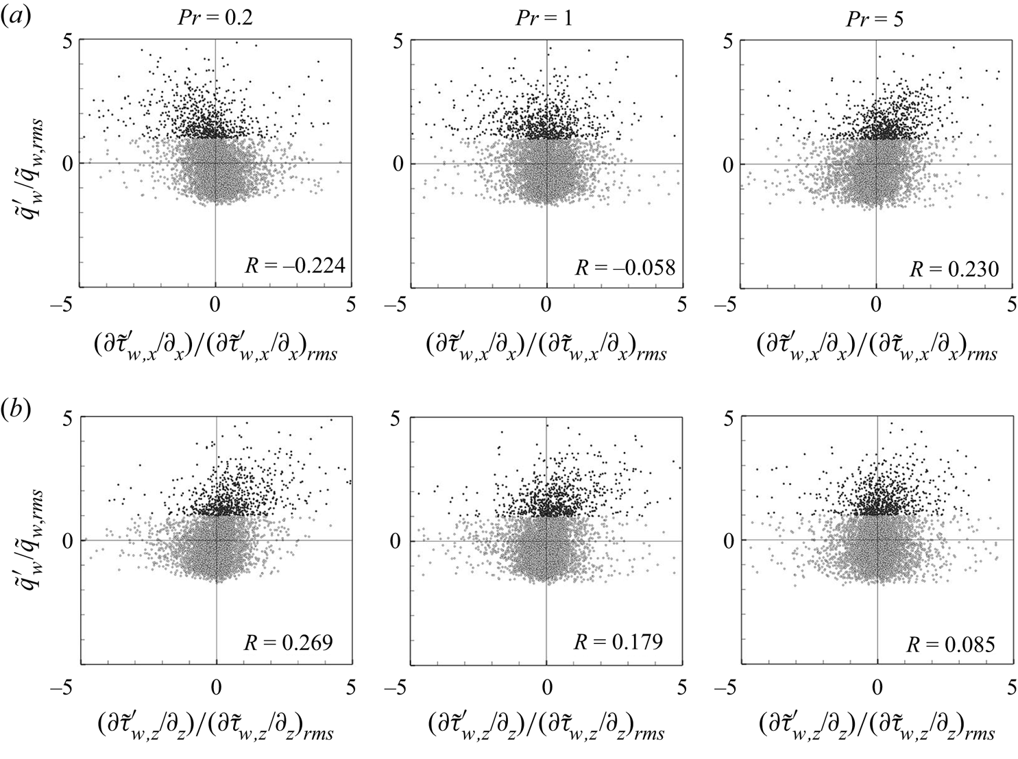
We discovered a strong correlation between the heat flux and gradient of the wall-shear stresses depending on  $Pr$ after a detailed investigation of the gradient map and its relation to the gradient of the wall-shear stresses for two example fields demonstrated in figures 14 and 15. For $Pr=0.2$, a strong heat flux occurs in the region with a negative streamwise gradient of the streamwise wall-shear stress or a positive spanwise gradient of the spanwise wall-shear stress. However, for $Pr=5$, the region of high heat flux is highly correlated with the region with a positive gradient of the streamwise wall-shear stress. When $Pr = 0.71$, a strong heat flux was found in the region with a strong streamwise wall-shear stress. The scatter plots between the normalized heat flux and the normalized gradient of the wall-shear stresses obtained from DNS for $Pr=0.2, 1$ and $5$, shown in figure 16, confirm this behaviour. The locally high heat flux ( $\tilde {q}'_w \geq \tilde {q}_{w,rms}$), marked by the black dot in figure 16(a), clearly indicates negative and positive correlations with the streamwise gradient of the streamwise wall-shear stress for $Pr=0.2$ and 5, respectively, while showing almost no correlation for $Pr=1$. A locally high heat flux, on the other hand, shows an overall positive correlation with the spanwise gradient of the spanwise wall-shear stress for $Pr \leq 1$, as shown in figure 16(b); however, the smaller the value of $Pr$, the stronger is the positive correlation. The correlation coefficients provided in figure 16 quantitatively support this behaviour, but less conspicuously, because all data points, including the data with negative fluctuations of heat flux, which do not have any correlation with the gradient of wall-shear stresses, were considered in the calculation of the correlation coefficient.
Scatterplots between surface heat flux with  $Pr$ and gradient of (a) streamwise wall-shear stress $\partial {\tilde {\tau }_{w,x}}/\partial {x}$ and (b) spanwise wall-shear stress ${\partial {\tilde {\tau }_{w,z}}}/\partial {z}$. High heat flux data ( $\tilde {q}'_w > \tilde {q}_{w,rms}$) are marked with darker points to highlight the correlation.
Recognizing that the gradient of the wall-shear stresses is associated with the near-wall flow structures, we propose plausible pictures by which the region with locally high heat flux is estimated from the flow behaviour, as presented in figure 17. A sweep and ejection event commonly observed in near-wall turbulence causes streamwise wall-shear stress distribution, as shown in figure 17(a). From our discussion of the correlation between the heat flux and streamwise wall-shear stress above, we can pinpoint the region of the local hotspot where high heat flux occurs, depending on  $Pr$, as shown in figure 17(a). This indicates that sweeping flow causes a high heat flux for $Pr >1$, whereas ejection flow induces a high heat flux for $Pr <1$. When $Pr =1$, high heat flux and strong streamwise shear tend to occur at the same location. A streamwise vortex also causes the spanwise wall-shear stress distribution shown in figure 17(b), from which a local hotspot can be identified from the correlation between the heat flux and the spanwise wall stress for $Pr < 1$. However, when $Pr >1$, a streamwise vortex does not contribute to a high heat flux.
Schematic for physical relationship between near-wall transport and heat transfer with the Prandtl number.
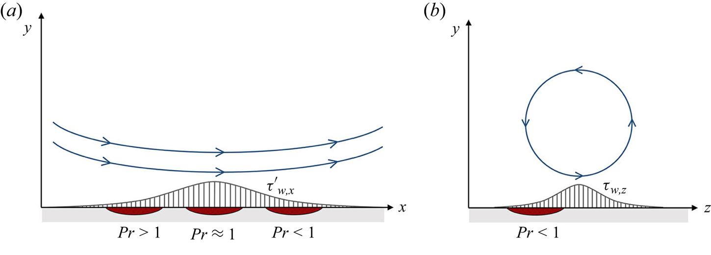
In summary, we demonstrated the interpretability of DL through an investigation of the gradient map between the input wall-shear stresses and output heat flux. Depending on the Prandtl number, the diverse physics of near-wall turbulent heat transfer can be identified.
3.3. Decomposition of Prandtl number effect
For efficient learning, we introduced decomposition of the surface heat flux ( $\tilde {q}_{w}=\tilde {q}_{w}^{C}+\tilde {q}_{w}^{P}$) into $Pr$-independent features ( $\tilde {q}_{w}^{C}$) and $Pr$-dependent features ( $\tilde {q}^{P}$) in the network, as discussed in § 2.2. In this section we investigate the behaviour of the features obtained using the trained model in § 3.2. The $Pr$-independent features contain common characteristics of the surface heat flux irrelevant to $Pr$, whereas the $Pr$-dependent features reflect the characteristics of the surface heat flux dependent on $Pr$. These decomposed features are automatically obtained through the training process by adopting GAN explained in § 2.2 without additional knowledge regarding the criterion of the data. Therefore, DL with a decomposition algorithm is a convenient and effective method for extracting decomposed physical features. A detailed analysis of the noticeable physical properties from the decomposed features aids in understanding the $Pr$ effect in turbulent heat transfer.
First, we investigate statistics such as the variance and correlation coefficient of the decomposed fields of the surface heat flux ( $\tilde {q}_{w}^{C}$ and $\tilde {q}_{w}^{P}$), as listed in table 3. By definition, the mean of $\tilde {q}_w$ is 1, whereas the mean of the $Pr$-independent feature $\langle \tilde {q}_{w}^{C}\rangle$ is approximately $1$, and that of $Pr$-dependent features $\langle \tilde {q}_{w}^{P}\rangle$ for all $Pr$ is negligibly small when the training network is constructed. The variance of the $Pr$-dependent feature is relatively small compared with that of the $Pr$-independent feature, which is comparable to the total heat flux, suggesting that the $Pr$-independent feature captures the common behaviour of the heat flux for all $Pr$. The high correlation coefficient between $\tilde {q}_w$ and $\tilde {q}_w^C$ for all $Pr$ values also supports this argument. On the other hand, $\tilde {q}_w^P$ is mildly correlated with $\tilde {q}_w$ but hardly correlated with $\tilde {q}_{w}^{C}$, indicating that the $Pr$-independent feature extracts common characteristics regardless of $Pr$. Furthermore, the high correlation coefficients between $\tilde {q}_w$ and $\tilde {q}_{w}^{C}$, and $\tilde {q}_w$ and $\tilde {q}_w^P$ for $Pr=0.71$ and 2, strongly suggest that the $Pr$-independent feature is most pronounced in the heat flux field for $Pr$ around 1.
Variance and correlation coefficient of the  $Pr$-independent feature, $Pr$-dependent feature and surface heat flux with trained $Pr$.
$Pr$.
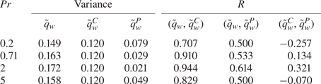
Figure 18 shows example snapshots of  $\tilde {q}_{w}^{C}$, $\tilde {q}_{w}^{P}$ and $\tilde {q}_w$ for the same input field for various values of $Pr$, with the contours of $\tilde {q}_{w}^{C}$ and $\tilde {q}_w$ displayed for values greater than 1. The strong correlation between $\tilde {q}_{w}^{C}$, $\tilde {q}_{w}^{P}$ and $\tilde {q}_w$, shown in table 3, suggests that the similarity between them is most pronounced for $Pr=0.71$ or 2. The only difference is that $\tilde {q}_w$ has higher peak values than $\tilde {q}_w^C$, as evidenced by the $\tilde {q}_w^P$ distribution, which has a positive correlation with $\tilde {q}_w^C$. When $Pr=0.2$ or 5, however, there are mismatches in the peak locations of $\tilde {q}_{w}^{C}$ and $\tilde {q}_w$ in the opposite sense, with $\tilde {q}_w$ peaks found slightly downstream and upstream of those of $\tilde {q}_w^C$ for $Pr=0.2$ and $Pr=5$, respectively. The opposite behaviour of the $\tilde {q}_w^P$ distributions for $Pr=0.2$ and 5 clearly confirms this. Another difference is that the high heat flux regions for $Pr=5$ are significantly elongated in the streamwise direction compared with those for $Pr=0.2$. This kind of shift in the peak locations is obviously caused by the different physical relationships between the surface heat flux and the flow field depending on $Pr$, as described in figure 17. The decomposition algorithm captured this difference.
Example fields of the  $Pr$-independent feature $\tilde {q}_w^C$ (line contours with levels from 1.0 to 3.0 with an increment of 0.2 in the left panels), $Pr$-dependent feature (colour contours in the left panels) and the total heat flux $\tilde {q}_w$ (line contours with levels from 1.0 to 3.0 with an increment of 0.2 in the right panels) for various $Pr$ decomposed through cGAN.

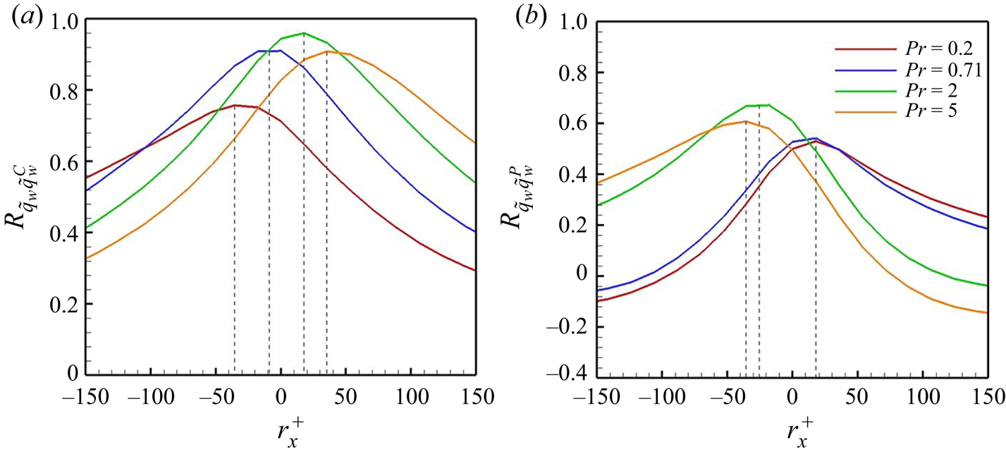
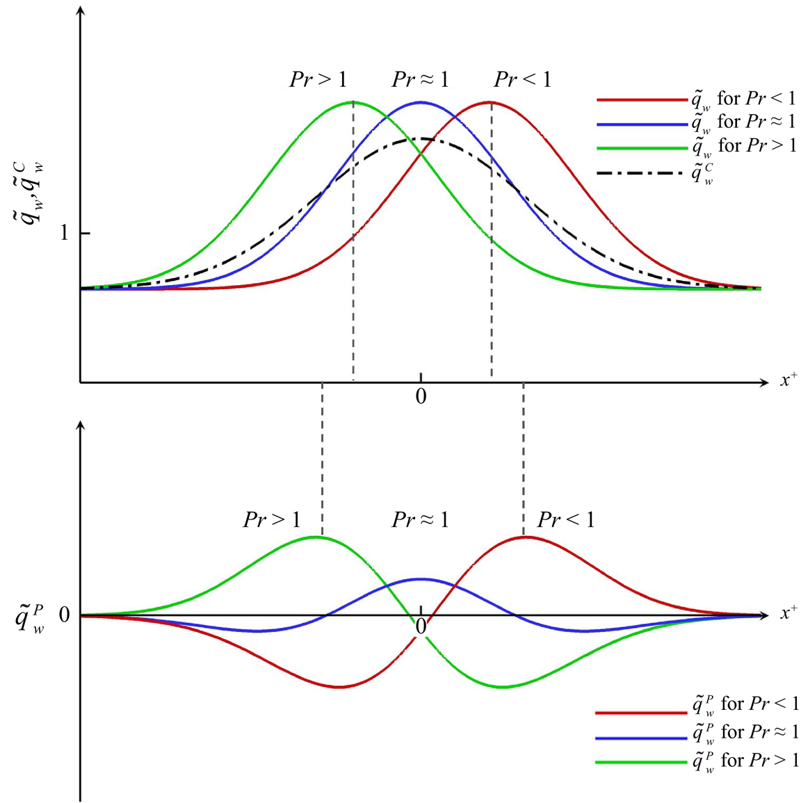
Figure 19 shows the two-point correlations along the streamwise direction  $R_{\tilde {q}_{w}\tilde {q}_{w}^C}(r_x)$ and $R_{\tilde {q}_{w}\tilde {q}_{w}^P}(r_x)$ for $Pr=0.2, 0.71, 2$ and 5, for a quantitative investigation of the spatial relationship between the local heat flux, $Pr$-independent feature and $Pr$-dependent feature. The surface heat flux for all $Pr$ has a high correlation with the $Pr$-independent feature, as confirmed by table 3, with peaks shifted at $-50< r_x^+<50$. The correlation peaks for $Pr=5$ and 2 are observed at approximately $r_x^+=35$ and 20, respectively, while those for $Pr=0.71$ and 0.2 are found at $r_x^+=-10$ and $-35$, indicating that the peak for $Pr \approx 1$ is located in the centre, and shifts downward/upward as $Pr$ increases/decreases. On the other hand, the surface heat flux for all $Pr$ shows a mild correlation with the $Pr$-dependent feature, as shown in figure 19(b). As $Pr$ varies, the correlation peaks shift in the opposite direction to that of the correlation between the surface heat flux and the $Pr$-independent feature shown in figure 19(a), but the amount of shift is smaller. Furthermore, the correlation is asymmetric and even becomes negative for large $r_x$ for $Pr > 1$ and for large $-r_x$ for $Pr < 1$. For a clear understanding of these correlations, we provide a schematic describing the plausible streamwise distribution of the typical normalized surface heat flux and the corresponding decomposed features for three ranges of $Pr$ in figure 20. Three distributions of locally high surface heat flux for each $Pr$ regime for the same flow field inferred from DNS data of the normalized surface heat flux shown in figure 18, which is consistent with the schematic in figure 17, are plotted in the upper panel of figure 20 along with the corresponding $Pr$-independent feature. The corresponding $Pr$-dependent features for each $Pr$ regime are displayed in the lower panel. This clearly explains the high correlation between the surface heat flux and the $Pr$-independent feature and the mild and asymmetric correlation between the surface heat flux and $Pr$-dependent feature. The shifts in the peak location of the two-point correlations shown in figure 19 are self-evident, and the negative correlation between the surface heat flux and the $Pr$-dependent feature for large distances can be explained by the schematic in figure 20. This also supports the necessity of the decomposition algorithm, because a major common part clearly exists among the locally high surface heat flux distribution, and the $Pr$-dependent components are clearly distinct.
Two-point correlations along the streamwise direction (a)  $R_{\tilde {q}_{w}\tilde {q}_{w}^C}(r_x)$ between surface heat flux $\tilde {q}_{w}$ and the $Pr$-independent feature $\tilde {q}_{w}^C$, and (b) $R_{\tilde {q}_{w}\tilde {q}_{w}^P}(r_x)$ between surface heat flux $\tilde {q}_{w}$ and the $Pr$-dependent feature $\tilde{q}_{w}^{P}$).
Schematics describing typical distributions of  $\tilde {q}_w$, $\tilde {q}_w^C$ and $\tilde {q}_w^P$ for the same flow field for three regimes of $Pr$. The vertical dashed lines indicate the different peak locations for $\tilde {q}_w$ and $\tilde {q}_w^P$.
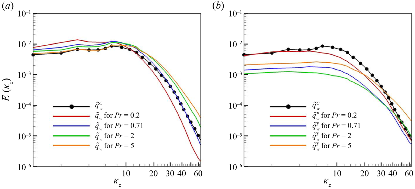
The  $Pr$-independent feature tends to capture the spanwise variation that is most similar to that for $Pr=0.71$, as shown in figure 18. The spanwise one-dimensional energy spectrum of the surface heat flux and the $Pr$-independent feature shown in figure 21(a) quantitatively confirms that the energy spectra of the $Pr$-independent feature and the surface heat flux for $Pr=0.71$ almost coincide in the high-wavenumber region, whereas the spectra in the low-wavenumber region for $Pr=5$ are similar. The $Pr$-dependent feature clearly has a lower energy level in the low-wavenumber region than the $Pr$-independent feature, except for $Pr = 0.2$, as shown in figure 21(b). It is noteworthy that the $Pr$-independent feature shows a peak at $\kappa _z = 7$, indicating the capture of the average spanwise spacing of the thermal streaks of 160 wall units for $Pr = 0.71, 2$ and 5, while the spacing for $Pr = 0.2$ and 360 wall units is not reflected. Correspondingly, the spectra of the $Pr$-dependent feature for $Pr = 0.71$, 2 and 5 monotonically decrease with the wavenumber, whereas the spectrum for $Pr=0.2$ shows a mild peak in the low-wavenumber range.
One-dimensional energy spectra for decomposed fields with  $Pr$. (a) Spanwise energy spectra of the $Pr$-independent feature ( $\tilde {q}_{w}^C$) and surface heat flux ( $\tilde {q}_{w}$). (b) Spanwise energy spectra of the $Pr$-independent feature ( $\tilde {q}_{w}^C$) and the $Pr$-dependent feature ( $\tilde {q}_{w}^P$).
In this section we demonstrated how our algorithm decomposes the surface heat flux into a  $Pr$-independent feature and $Pr$-dependent features during the training process. For the considered range of $Pr$, this decomposition clearly confirms that there exists a common feature in the high heat flux events, but the $Pr$-dependent features are quite distinct. By investigating the correlation between these features, we explored the effect of the Prandtl number in determining their physical relationship with the surface heat flux.
4. Conclusion
We developed a NN combining cGAN with a decomposition algorithm to predict the Prandtl number effect on the surface heat flux in a turbulent channel flow. The trained model could accurately predict the local heat flux for any Prandtl number within the trained range based only on the wall-shear stresses. The physical interpretation of the DL model using the gradient map allowed us to better understand the characteristics of the surface heat flux depending on the Prandtl number than on the spatial correlation between the input and output. Furthermore, we investigated the effect of the Prandtl number by observing the decomposed features obtained using our model.
First, we evaluated the predictive performance of the developed cGAN compared with that of the CNN and a multiple-linear model. The cGAN predicted the surface heat flux for the untrained  $Pr$ with almost the same accuracy as for the trained $Pr$. Some statistics, such as $Nu$ and r.m.s. predicted by cGAN and CNN, almost matched those of DNS, whereas the multiple-linear model showed large errors. In high-order statistics, such as skewness and flatness, cGAN tends to underpredict slightly compared with low-order statistics, but shows better performance than other models. For the PDF of the surface heat flux, our model was able to predict locally high values of surface heat flux for both trained and untrained $Pr$. On the other hand, the CNN showed a large error at high values of surface heat flux. In the energy spectra of the surface heat flux for the trained $Pr$, cGAN slightly underestimated the energy of DNS but performed better than the CNN. In the energy spectra for the untrained $Pr$, our model was slightly inaccurate compared with those for the trained $Pr$, but the model performed similarly or slightly better than the CNN.
Through gradient maps obtained using the trained model, we investigated the physical relationship between the wall-shear stresses and surface heat flux. Because of the presence of noise, the average gradient maps for various ranges of  $Pr$ were studied. We observed that the positive peak of the average gradient map for the streamwise wall-shear stress is located in the upstream region for $Pr<1$ and in the downstream region for $Pr>1$. The average gradient map for the spanwise wall-shear stress was pronounced only for $Pr <1$ and showed positive peaks in the first and third quadrants and negative peaks in the second and fourth quadrants. This pattern implies that the local heat flux can be stronger when a pair of vortices exist downstream or when a vortex crosses diagonally. In addition, for a more detailed analysis, we examined the instantaneous gradient map with minimized noise using symmetry and homogeneity. From an investigation of two sample fields showing strong heat flux, we discovered that the streamwise gradient of the streamwise wall-shear stress was selectively strongly correlated with the surface heat flux. Furthermore, the spanwise gradient of the spanwise wall-shear stress is correlated with the surface heat flux only when $Pr<1$. These observations strongly suggest that the hotspot, that is, the locally high heat flux region, is mostly found in the sweeping region for $Pr>1$ and in the ejection region for $Pr<1$. The hotspot can also be found in the down-flow region near a streamwise vortex for $Pr<1$. From a detailed analysis of the gradient map obtained from the trained model, we clearly showed that a physical interpretation of the DL model is indeed possible.
Finally, we analysed the effect of the Prandtl number by observing the decomposed fields of the surface heat flux and the  $Pr$-independent and $Pr$-dependent features obtained from cGAN. Although the surface heat flux exhibits a peak at different locations depending on the Prandtl number, a common characteristic is clearly captured by the $Pr$-independent feature. The $Pr$-dependent features for different Prandtl numbers exhibit distinct distributions. The two-point correlation between the surface heat flux, the $Pr$-independent feature and the $Pr$-dependent feature indicates that the shifts of peaks in the two-point correlation between them can be explained by the high heat flux region for the sweep and ejection events found in the analysis of the gradient map. The effectiveness of the decomposition algorithm adopted in our study for training and in-depth interpretation was demonstrated.
The limitations of the current approach are also discussed. The decomposition algorithm separating the parameter-dependent component from the common component works well only when the common part clearly exists in the non-negligible portion of the data within the considered range. Otherwise, the learning process could be unstable and the performance could be poor. Another factor that might be critical for successful learning is the scaling property of the turbulence data, particularly the output of the DL algorithm. Fortunately, the surface heat flux has a good scaling property for the considered range of parameters; both the mean and r.m.s. values scale  $\sim Pr^{1/2}$ (see figure 2). This property was exploited in the normalization of the output of the learning network, which helped in stable learning and proper performance of the decomposition algorithm. However, in situations where such a nice scaling property is unavailable, successful learning cannot be guaranteed. The gradient map, which was used in the interpretation of the trained network, is known for its noisy nature because the network is strongly nonlinear and the learning is based on statistical data. Averaging over various data can eliminate noise, but there is loss of detailed information. In our analysis, we suppressed the noise in the instantaneous gradient map using symmetry or homogeneity. However, these properties may not be applicable in other problems. In this study we focused on the effect of the Prandtl number in the predictability and analysis of the DL models. The effect of the Reynolds number would be an interesting topic for extension of the current approach, particularly given that deviations from the Reynolds analogy are another meaningful and worthwhile issue for investigation.
In this study we clearly demonstrated that unified DL combining cGAN and the decomposition algorithm can predict the surface heat flux for various Prandtl numbers based on the wall-shear information and provided a physical interpretation of the trained network using the gradient map, which can identify the Prandtl number effect in turbulent heat transfer. The developed decomposition algorithm can be extended to the analysis of the effects of other physical parameters such as the Reynolds number. Through a careful investigation of the trained network, we provide evidence that the physical interpretation of DL is indeed possible.
Funding
This work was supported by the National Research Foundation of Korea (NRF) Grant funded by the Korean Government MSIT (2022R1A2C2005538).
Declaration of interests
The authors declare that they have no conflicts of interest.
Appendix A. Architecture of conditional generate adversarial networks
The network architecture of cGAN with a decomposition algorithm is presented in figure 22. Our model consists of a generator and discriminator, and the generator is divided into two parts: a parameter-independent and parameter-effect generator. Figures 22(a) and 22(b) show the parameter-independent generator ( $G^{C}$) and the parameter-effect generator ( $G^{P}$) in the generator ( $G$), respectively, and figure 22(c) shows the discriminator. Here $G^{C}$ takes as inputs the wall-shear stresses, streamwise and spanwise shear stresses, and generates $Pr$-independent features as outputs; $G^{P}$ predicts the $Pr$-dependent features using $Pr$-independent features, wall-shear stresses and the Prandtl number. Finally, the surface heat flux for $Pr$ can be obtained by adding $Pr$-independent and $Pr$-dependent features. For $G^{C}$ and $G^{P}$, skip connections with $n\times n$ downsampling are applied for efficient learning of large-scale structures, and the number of layers and feature maps are the same. The size of the discrete convolution (Conv. in figure 22) is $3\times 3$, and the sizes of both upsampling and downsampling are $2\times 2$. For the discriminator, the input data are the wall-shear stresses, surface heat flux and the Prandtl number, and the sizes of convolution and downsampling are $3\times 3$ and $2\times 2$, respectively. The last two layers are fully connected (FC in figure 22c). The batch size and the total number of iterations were 16 and 500 000, respectively, and the learning rate was fixed at 0.0001. The Adam optimizer suggested by Kingma & Ba (Reference Kingma and Ba2014) was applied to update the weights, and the initialization suggested by He et al. (Reference He, Zhang, Ren and Sun2015) was used for the initial weights. For comparative models in § 3.1, the architecture of the CNN and multiple-linear models is only the generator ( $G$), including $G^{C}$ and $G^{P}$, of the cGAN, and the shallow CNN consists of two convolution layers with the 16 hidden feature maps and the leaky ReLU function. The multiple-linear models adopted a linear function instead of the leaky ReLU function.
Network architectures for cGAN. (a) Parameter-independent generator ( $G^C$) and (b) parameter-effect generator ( $G^P$) in generator ( $G$). (c) Discriminator ( $D$).
$D$).
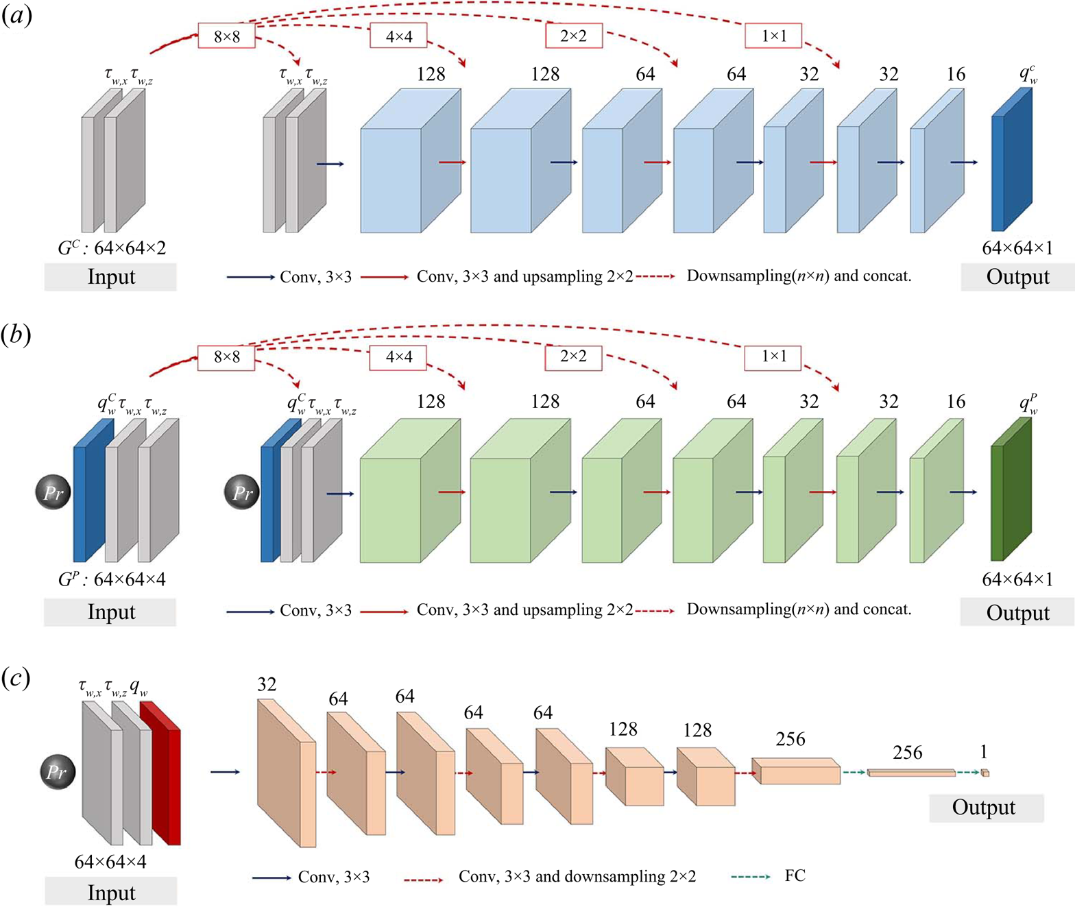
Appendix B. Training process of conditional generative adversarial networks
In order to confirm the training convergence of cGAN, the training and validation errors of the normalized surface heat flux  $\tilde {q}_{w}$ for trained $Pr$ are presented in figure 23. The training and validation data are 1000 and 100 fields with $\Delta t^+=9$, respectively, where the validation data are sufficiently decorrelated with the training data. Mean squared loss is obtained using subregions $(64\times 64)$ for all training and validation datasets every 1000 iterations, and the total number of iterations is 500 000. In the training process cGAN showed the lowest error for $Pr = 0.71$ and $2$, but a relatively larger error is observed for $Pr = 5$ than other Prandtl numbers. However, for all Prandtl numbers, the training and validation errors are almost similar, indicating that our network model does not overfit the training data.
Training and validation errors of surface heat flux  $\tilde {q}_{w}$ for trained $Pr(=0.2, 0.71, 2, 5)$.
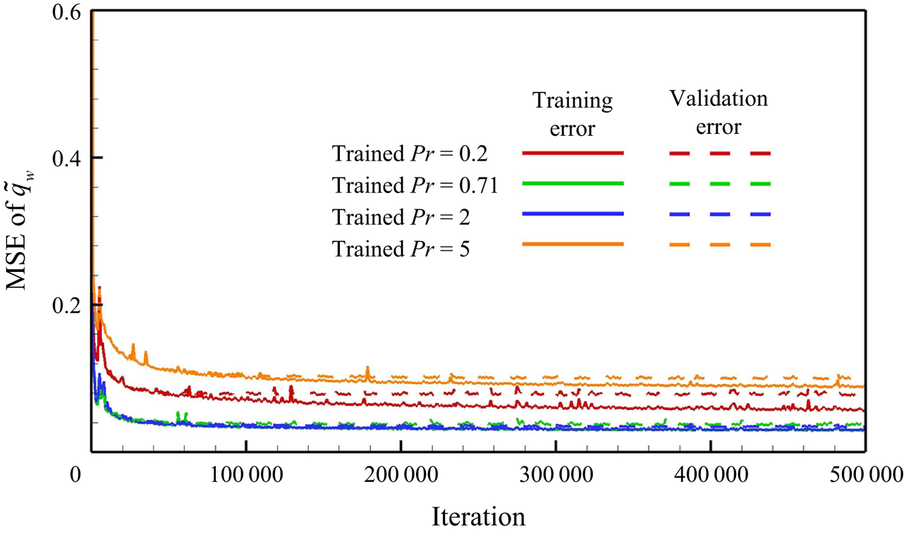
Appendix C. Prediction of surface heat flux at low Prandtl numbers
In this section we describe the performance of the cGAN in predicting the surface heat flux at low Prandtl numbers from the wall-shear stresses. The trained  $Pr$ values are 0.005, 0.01 and 0.025, and the untrained $Pr$ values are 0.001 and 0.05. We collected from DNS the wall-shear stresses and surface heat flux fields at every $\Delta t^+=9$. The numbers of training and validation data fields for trained $Pr$ are 1000 and 100, respectively. The number of testing data fields for all $Pr$ is 1000. The untrained data were collected far from the training data. To train the DL, the surface heat flux for $Pr$ and the wall-shear stresses were normalized by their own mean and standard deviation, respectively. In the training process the input and output data in the subregion ( $64 \times 64$) in the $x$–
$x$– $z$ plane were randomly sampled. Before presenting the prediction performance, we investigate the probability density function of the heat flux for low $Pr$ using the DNS data in figure 24. As $Pr$ decreased, the surface heat flux approached a Gaussian distribution. In addition, the fluctuations became very small, and a strong local heat flux was rarely observed. As shown in figure 2(a), the Nusselt number is close to 1, which is the Nusselt number for the pure conduction state for the considered range of $Pr$, suggesting that the role of turbulence in enhancing the heat transfer is minimal.
Probability density function (p.d.f.) of surface heat flux for low  $Pr$ obtained using DNS.
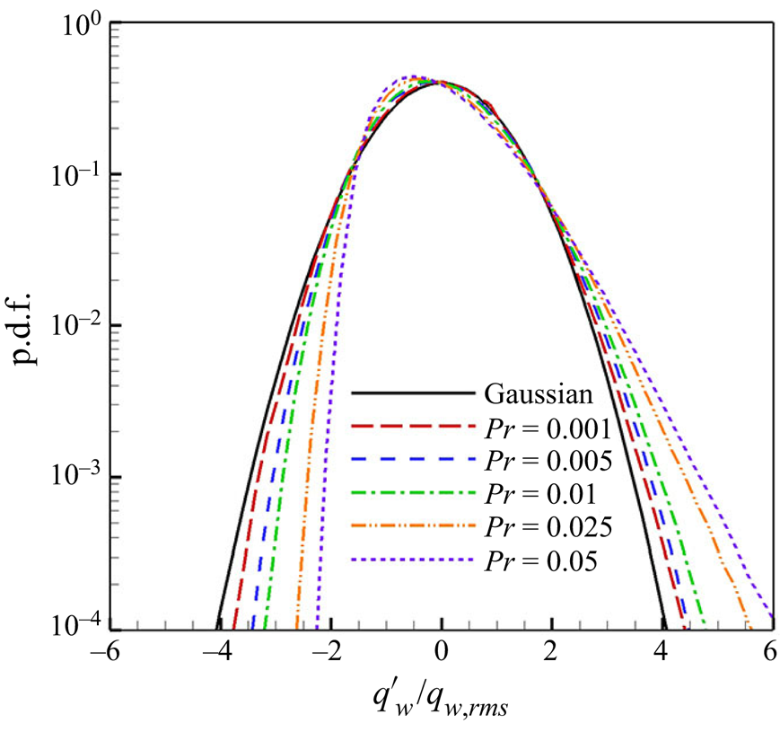
In figure 25 the surface heat flux fields for the trained and untrained  $Pr$ predicted using the trained cGAN are showed and compared with DNS data. The predicted local heat flux at $Pr=0.01$ is slightly underpredicted compared with DNS, but the overall predicted heat flux field shows a distribution similar to that of DNS. For untrained $Pr$, our model somewhat underpredicted the local heat flux compared with that of DNS, but the generated field was qualitatively similar to that of DNS.
Instantaneous surface heat flux for low  $Pr$ obtained from wall-shear stresses using cGAN.
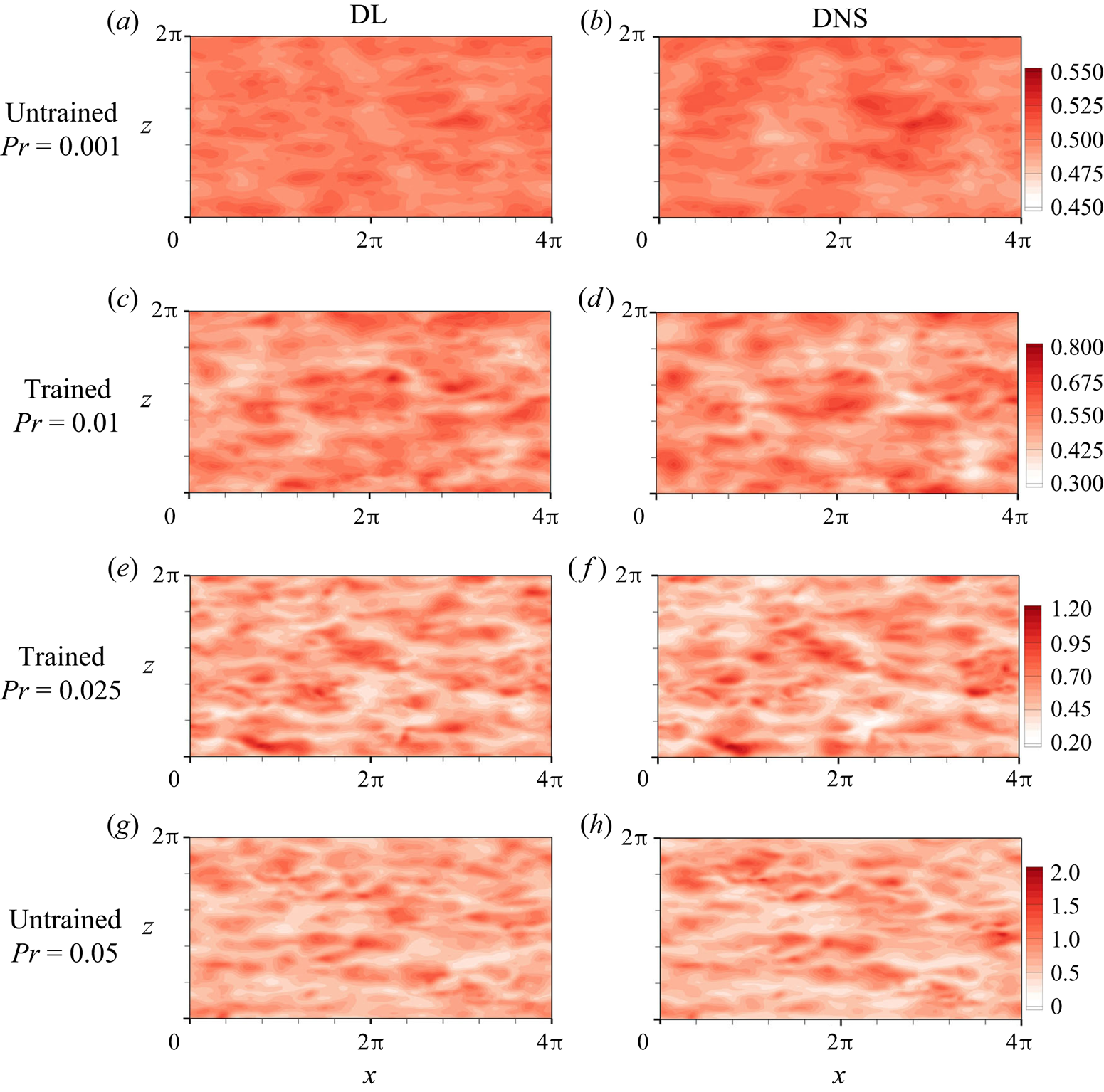
The basic statistics of the predicted surface heat flux, such as the mean, r.m.s., skewness and flatness for both the trained and untrained  $Pr$, are presented in figure 26. As shown in figure 26(a), the behaviour of $Nu$ approaching 1 with decreasing $Pr$ is accurately predicted for both trained and untrained $Pr$. Our model predicts r.m.s. with some error, even for the trained $Pr$, but the decreasing trend with Prandtl number is well captured. As shown in figure 26(b), the skewness of the surface heat flux monotonically decreased with decreasing $Pr$, whereas the flatness approached 3, indicating that the surface heat flux approached a Gaussian distribution. These behaviours were well predicted by cGAN although, for $Pr=0.001$, a small value of skewness was overpredicted.
Statistics of surface heat flux ( $q_{w}$) for trained $Pr$ ( $=0.005, 0.01, 0.025$) and untrained $Pr$ ( $=0.001, 0.05$) predicted through cGAN; (a) $Nu$ and r.m.s., (b) skewness and flatness.
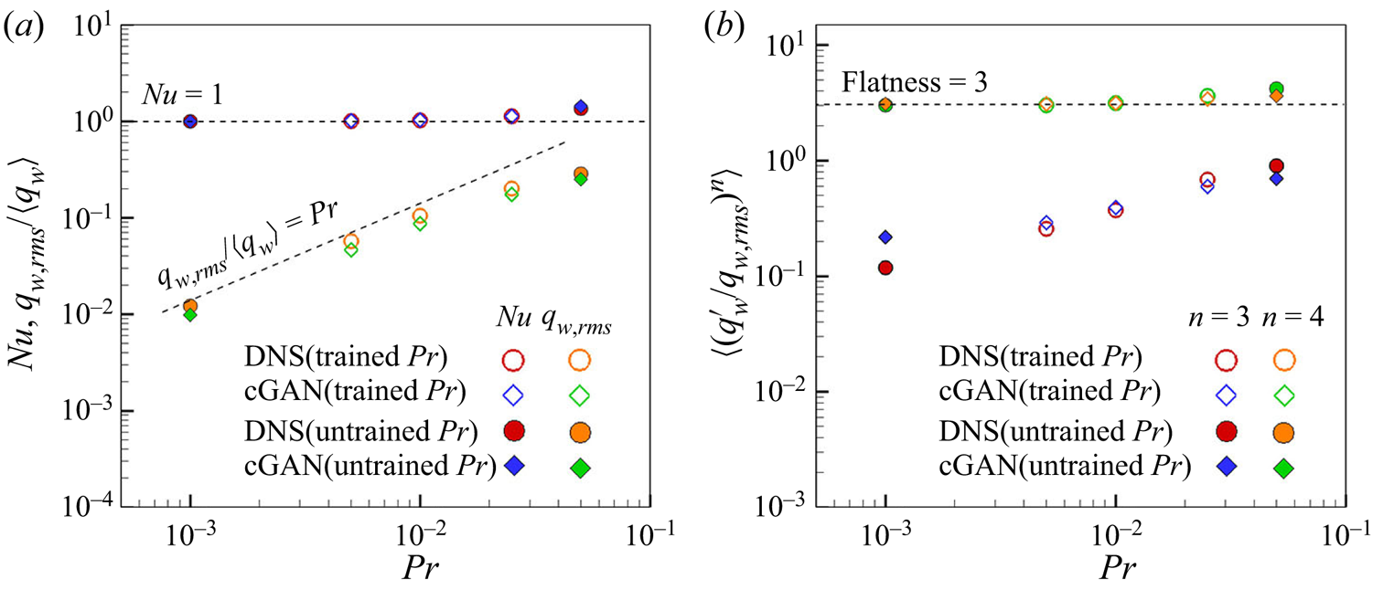
Finally in figure 27, we show the energy spectrum of the surface heat flux for trained  $Pr$. In both the streamwise and spanwise energy spectra, cGAN underpredicts DNS data at low wavenumbers and shows a noisy kink near the highest wavenumber. The streamwise and spanwise spectra appear similar for the smallest $Pr (=0.001)$ considered, in the sense that $E(\kappa _x) \simeq E(\kappa _z =\kappa _x/2)$, implying extended isotropy, though this trend becomes less pronounced as $Pr$ increases. No such trend was observed in the behaviour of the surface heat flux for high values, i.e. when $Pr>0.1$ (see figure 9).
One-dimensional energy spectra of surface heat flux ( $q_{w}$) for trained $Pr$ ( $=0.005, 0.01, 0.025$) and untrained $Pr$ ( $=0.001,0.05$) predicted through cGAN. (a) Streamwise and (b) spanwise energy spectra.
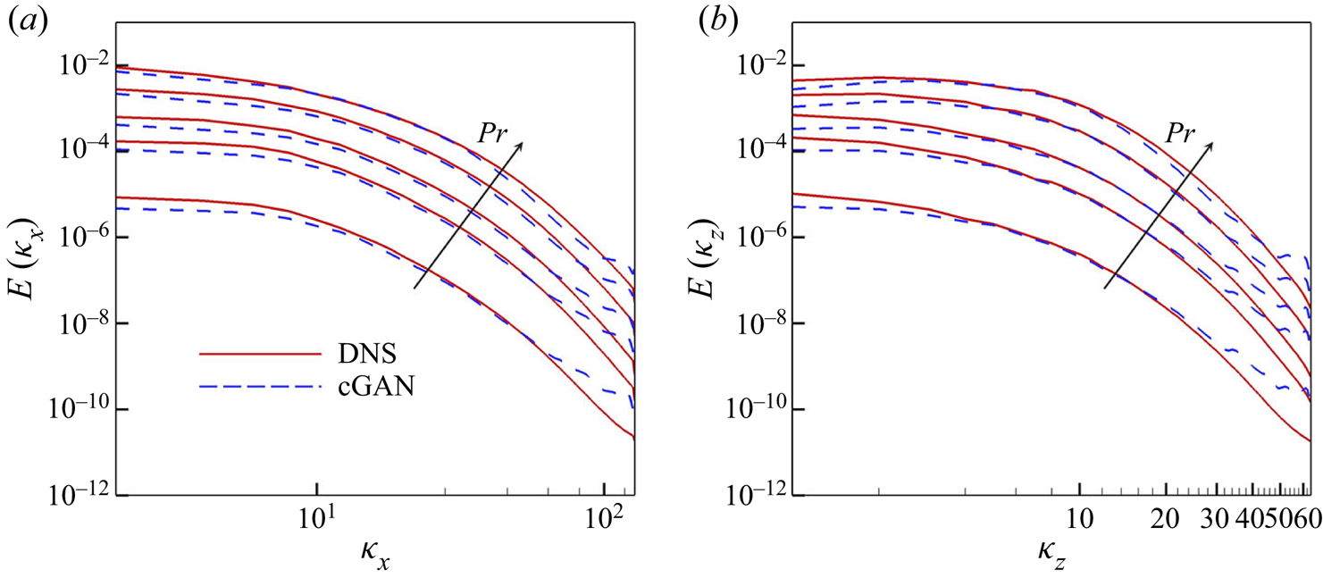
Appendix D. Pressure effect for prediction of surface heat flux
In this section we investigate the role of wall pressure in the prediction of the surface heat flux when it is considered as extra input information. In this test the prediction model of the surface heat flux, training process and the number of paired data were kept the same as those described in § 3.1. The correlation coefficient between the target DNS data and the predicted surface heat flux obtained using pressure as an extra input, as listed in table 4, shows a slight improvement compared with the cases without pressure for both the trained and untrained  $Pr$. Although not presented here, there was no significant improvement in the accuracy of higher-order statistics such as the energy spectrum and PDF of the surface heat flux.
Correlation coefficient between target data (DNS data) and surface heat flux with  $Pr$ predicted by cGAN with/without pressure information.

The marginal improvement using the pressure information suggests that the wall pressure information is redundant in the prediction of the surface heat flux. It is known that the spanwise gradient of wall pressure fluctuations is strongly correlated with the spanwise wall-shear stress (Kim Reference Kim1989). As shown in figures 28(a) and 28(b), the wall pressure fluctuations exhibit a positive correlation with the spanwise gradient of the spanwise wall-shear stress, and the gradient of the pressure fluctuations is strongly correlated with the spanwise wall-shear stress. This correlation can be understood by the schematic presented in figure 28(c), in which both the high- and low-pressure regions on the surface and the spanwise wall-shear stress can be caused by fluid motion associated with a streamwise vortex. Therefore, the addition of pressure to the input did not significantly affect the prediction of the surface heat flux.
Scatterplots (a) between the spanwise gradient of spanwise wall-shear stress  ${\partial {\tilde {\tau }_{w,z}}}/\partial {z}$ and pressure fluctuation $\tilde {p}$, and (b) between the spanwise wall-shear stress $\tilde {\tau }_{w,z}$ and the gradient of pressure fluctuation ${\partial {\tilde {p}}}/\partial {z}$. (c) Schematic for physical relationship between spanwise wall-shear stress and pressure fluctuations.
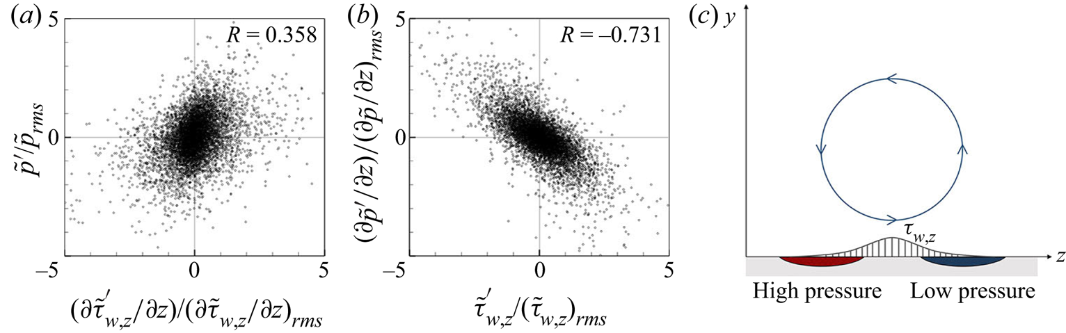
Finally, we investigated whether the interpretability of the trained cGAN is influenced by adding pressure fluctuations to the input through the average gradient map, which was obtained with pressure input in the same way as described in § 3.2. The average gradient maps of the streamwise wall-shear stress, spanwise wall-shear stress and pressure fluctuations are shown in figures 4(a), 4(b) and 4(c), respectively. The gradient maps of the wall-shear stresses are almost similar to those of the trained cGAN without pressure (see figure 12) for most values of  $Pr$, except for the gradient map of the spanwise wall-shear stress for $Pr=0.2$, which shows a slight shift in the peaks in the upstream direction compared with the case without pressure. The gradient map of the pressure for $Pr=0.2$ shows a strong negative peak at the centre, as shown in figure 29(c). Given the correlation between the pressure and spanwise gradient of the spanwise shear stress shown in figure 28(a), the role of pressure is to mitigate the effect of the spanwise shear stress in determining the surface heat flux. Therefore, the wall pressure information did not substantially contribute to an improvement in the prediction accuracy of the surface heat flux.
Average gradient maps of surface heat flux  $\tilde {q}_{w}$ with respect to (a) streamwise wall-shear stress $\tilde {\tau }_{w,x}$, (b) spanwise wall-shear stress $\tilde {\tau }_{w,z}$ and (c) pressure fluctuations $\tilde {p}$ for $Pr$ obtained through cGAN.


 Open access

