





1. Introduction
1.1. Hyperbolic Brownian motion
The hyperbolic plane $\mathbb{H}^2$
is the unique complete, simply connected two-dimensional Riemannian manifold with constant curvature
$\mathbb{H}^2$
is the unique complete, simply connected two-dimensional Riemannian manifold with constant curvature $-1$
. A point
$-1$
. A point $o \in \mathbb{H}^2$
is distinguished as the origin, and the hyperbolic distance
$o \in \mathbb{H}^2$
is distinguished as the origin, and the hyperbolic distance $d_\mathbb{H}$
equips
$d_\mathbb{H}$
equips $\mathbb{H}^2$
with a norm and a metric. For distinct points
$\mathbb{H}^2$
with a norm and a metric. For distinct points $x, y \neq o$
, there are unique hyperbolic geodesics between o, x and between o, y, and these geodesics subtend an angle at o which is zero only if x lies on the geodesic from o to y, or vice versa. Every point
$x, y \neq o$
, there are unique hyperbolic geodesics between o, x and between o, y, and these geodesics subtend an angle at o which is zero only if x lies on the geodesic from o to y, or vice versa. Every point $x \in \mathbb{H}^2 \setminus \{ o \}$
can be represented in geodesic polar coordinates
$x \in \mathbb{H}^2 \setminus \{ o \}$
can be represented in geodesic polar coordinates $ x = (r,\theta)$
, where
$ x = (r,\theta)$
, where $r = d_\mathbb{H} (o, x) \in (0,\infty)$
, and
$r = d_\mathbb{H} (o, x) \in (0,\infty)$
, and $\theta \in [0,2\pi)$
is an angle relative to a fixed reference direction.
$\theta \in [0,2\pi)$
is an angle relative to a fixed reference direction.
Hyperbolic Brownian motion is a stochastic process $B\,:\!=\,(B_t)_{t \in {\mathbb R}_+}$
on
$B\,:\!=\,(B_t)_{t \in {\mathbb R}_+}$
on $\mathbb{H}^2$
, started from
$\mathbb{H}^2$
, started from $B_0 \,:\!=\, o$
, whose dynamics can be described in geodesic polar coordinates
$B_0 \,:\!=\, o$
, whose dynamics can be described in geodesic polar coordinates $B_t = (R_t, \theta_t) \in {\mathbb R}_+ \times [0,2\pi)$
,
$B_t = (R_t, \theta_t) \in {\mathbb R}_+ \times [0,2\pi)$
, $t > 0$
. The
$t > 0$
. The ${\mathbb R}_+$
-valued radial process
${\mathbb R}_+$
-valued radial process $R \,:\!=\, (R_t)_{t \in{\mathbb R}_+}$
starts from
$R \,:\!=\, (R_t)_{t \in{\mathbb R}_+}$
starts from $R_0\,:\!=\,0$
and satisfies the autonomous stochastic differential equation (SDE), in which
$R_0\,:\!=\,0$
and satisfies the autonomous stochastic differential equation (SDE), in which $W^R$
is a standard
$W^R$
is a standard $\mathbb{R}$
-valued Brownian motion,
$\mathbb{R}$
-valued Brownian motion,
 \begin{equation} \mathrm{d}R_t = \frac{\mathrm{d}t}{2\tanh R_t} + \mathrm{d}W_t^R \quad \text{for all } t \in {\mathbb R}_+.\end{equation}
Since $B_0 = o$
, the angle
$B_0 = o$
, the angle $\theta_0$
is not canonically defined, but for
$\theta_0$
is not canonically defined, but for $t \geq s > 0$
the increment
$t \geq s > 0$
the increment $\theta_t - \theta_s$
is described via an
$\theta_t - \theta_s$
is described via an $\mathbb{R}$
-valued post-s winding process
$\mathbb{R}$
-valued post-s winding process $\Theta^{(s)} \,:\!=\, (\Theta^{(s)}_t)_{t \geq s}$
which starts from
$\Theta^{(s)} \,:\!=\, (\Theta^{(s)}_t)_{t \geq s}$
which starts from $\Theta^{(s)}_s \,:\!=\,0$
and satisfies the SDE
$\Theta^{(s)}_s \,:\!=\,0$
and satisfies the SDE
 \begin{equation} \mathrm{d}\Theta^{(s)}_t = \frac{\mathrm{d}W^{(s)}_t}{\sinh R_t} \quad \text{for all } t \geq s,\end{equation}
where $W^{(s)}$
is a standard Brownian motion, independent of
$W^{(s)}$
is a standard Brownian motion, independent of $W^R$
. Then
$W^R$
. Then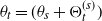 $\theta_t = ( \theta_s + \Theta^{(s)}_t )$
modulo
$\theta_t = ( \theta_s + \Theta^{(s)}_t )$
modulo $2\pi$
. Combined with the entrance law
$2\pi$
. Combined with the entrance law $\theta_s \sim \mathrm{Unif}\mkern2mu [0,2\pi)$
, for every
$\theta_s \sim \mathrm{Unif}\mkern2mu [0,2\pi)$
, for every $s >0$
, inevitable thanks to the rapid spinning out from the origin [Reference Itô and McKean21, Section 7.16], the SDEs (1) and (2) provide a unique-in-law description. In particular, the law of B is rotationally invariant. This also gives a skew product decomposition of Brownian motion on
$s >0$
, inevitable thanks to the rapid spinning out from the origin [Reference Itô and McKean21, Section 7.16], the SDEs (1) and (2) provide a unique-in-law description. In particular, the law of B is rotationally invariant. This also gives a skew product decomposition of Brownian motion on $\mathbb{H}^2$
, similarly to Euclidean Brownian motion in
$\mathbb{H}^2$
, similarly to Euclidean Brownian motion in $\mathbb{R}^d$
,
$\mathbb{R}^d$
, $d \geq 2$
. Note that from (1) it can be shown that
$d \geq 2$
. Note that from (1) it can be shown that $R_t >0$
for all
$R_t >0$
for all $t >0$
, almost surely (a.s.; see Lemma 4) so that in (2),
$t >0$
, almost surely (a.s.; see Lemma 4) so that in (2), $\sinh R_t > 0$
for
$\sinh R_t > 0$
for $t>0$
. (Started instead from
$t>0$
. (Started instead from $B_0 \neq o$
, there is no issue with
$B_0 \neq o$
, there is no issue with $\theta_0$
or rapid spinning, and (2) can be used to define the post-0 winding process
$\theta_0$
or rapid spinning, and (2) can be used to define the post-0 winding process $\Theta^{(0)}$
for all time.) For background on Brownian motion on
$\Theta^{(0)}$
for all time.) For background on Brownian motion on $\mathbb{H}^2$
, including the above facts, we refer to [Reference Rogers and Williams34, Section V.36] and [Reference Gruet15, Section 2], for example.
$\mathbb{H}^2$
, including the above facts, we refer to [Reference Rogers and Williams34, Section V.36] and [Reference Gruet15, Section 2], for example.
The following result, part of which is well known (see Remark 1), shows that hyperbolic Brownian motion B exhibits ballistic transience and a random limiting direction. It quantifies the intuition, apparent from (1), that since $\lim_{x \to \infty} \tanh x = 1$
, a comparison for the process R at large scales is a Brownian motion with a constant drift
$\lim_{x \to \infty} \tanh x = 1$
, a comparison for the process R at large scales is a Brownian motion with a constant drift $\frac12$
.
$\frac12$
.
Proposition 1. Almost surely,
 \begin{equation} \text{sup}_{t \in{\mathbb R}_+} \Bigl| R_t - W_t^R - \frac{t}{2} \Bigr| < \infty \quad \textit{and} \quad \lim_{t\to\infty}\frac{R_t}{t} = \lim_{t \to \infty} \frac{\mathbb{E}\,R_t}{t} = \frac{1}{2}. \end{equation}
Moreover, there exists a random variable $\theta_\infty$
, with
$\theta_\infty$
, with $\theta_\infty \sim \mathrm{Unif}\mkern2mu [0,2\pi)$
, and, for every
$\theta_\infty \sim \mathrm{Unif}\mkern2mu [0,2\pi)$
, and, for every $s >0$
, a random variable
$s >0$
, a random variable $\Theta_\infty^{(s)} \in \mathbb{R}$
, such that
$\Theta_\infty^{(s)} \in \mathbb{R}$
, such that
 \begin{equation} \lim_{t \to \infty}\theta_t = \theta_\infty\quad \textit{a.s.} \quad \textit{and, for every }s >0,\quad \lim_{t \to \infty}\Theta^{(s)}_t = \Theta^{(s)}_\infty \quad \textit{a.s.} \end{equation}
Moreover, for every $s>0$
,
$s>0$
,
 \begin{equation} \limsup_{t \to \infty} t^{-1} \log \bigl| \Theta^{(s)}_\infty - \Theta^{(s)}_t \bigr| = \limsup_{t \to \infty} t^{-1} \log | \theta_\infty - \theta_t | = -\frac{1}{2} \quad \textit{a.s.} \end{equation}
Remark 1. The strong law $\big(\!\lim_{t\to\infty} t^{-1} R_t = \frac12\big)$
, and the limiting direction (
$\big(\!\lim_{t\to\infty} t^{-1} R_t = \frac12\big)$
, and the limiting direction ( $\lim_{t \to \infty} \theta_t$
exists and is uniform) results are both well known, and some or all elements can be found, for example, in each of [Reference Pinsky33, Section V], [Reference Gruet15, Theorem 2.3], [Reference Rogers and Williams34, Section V.36], and [Reference Shiozawa35]. However, we were unable to find in the literature either the quantification of the angular convergence in (5), which says, roughly speaking, that
$\lim_{t \to \infty} \theta_t$
exists and is uniform) results are both well known, and some or all elements can be found, for example, in each of [Reference Pinsky33, Section V], [Reference Gruet15, Theorem 2.3], [Reference Rogers and Williams34, Section V.36], and [Reference Shiozawa35]. However, we were unable to find in the literature either the quantification of the angular convergence in (5), which says, roughly speaking, that $\theta$
converges at a rate subsequentially no better than
$\theta$
converges at a rate subsequentially no better than $\mathrm{e}^{-t(1+o(1))/2}$
, or the convergence of
$\mathrm{e}^{-t(1+o(1))/2}$
, or the convergence of $\mathbb{E}\,R_t$
in (3). Since these parts of the result are particularly relevant for us (cf. (6)). and to make the current paper more self-contained, we prove Proposition 1 in Section 5.
$\mathbb{E}\,R_t$
in (3). Since these parts of the result are particularly relevant for us (cf. (6)). and to make the current paper more self-contained, we prove Proposition 1 in Section 5.
1.2. The convex hull and its perimeter length
The trajectory $B[0,t] \,:\!=\, \{ B_s \colon s \in [0,t] \}$
of hyperbolic Brownian motion up to time
$B[0,t] \,:\!=\, \{ B_s \colon s \in [0,t] \}$
of hyperbolic Brownian motion up to time $t \in {\mathbb R}_+$
is a random compact subset of
$t \in {\mathbb R}_+$
is a random compact subset of $\mathbb{H}^2$
containing the origin o; the subject of our work is the closed convex hull
$\mathbb{H}^2$
containing the origin o; the subject of our work is the closed convex hull $\mathcal{H}_t \,:\!=\, \mathrm{conv}\,B[0,t]$
for
$\mathcal{H}_t \,:\!=\, \mathrm{conv}\,B[0,t]$
for $t \in {\mathbb R}_+$
, the smallest closed convex subset of
$t \in {\mathbb R}_+$
, the smallest closed convex subset of $\mathbb{H}^2$
containing B[0, t]. Recall that a set
$\mathbb{H}^2$
containing B[0, t]. Recall that a set $A \subseteq \mathbb{H}^2$
is convex if and only if, for every pair of distinct points
$A \subseteq \mathbb{H}^2$
is convex if and only if, for every pair of distinct points $x,y \in A$
, the (unique) hyperbolic geodesic between x and y is contained in A. Then
$x,y \in A$
, the (unique) hyperbolic geodesic between x and y is contained in A. Then $\mathrm{conv}\,S$
, for
$\mathrm{conv}\,S$
, for $S \subseteq \mathbb{H}^2$
, is the intersection of all closed convex sets
$S \subseteq \mathbb{H}^2$
, is the intersection of all closed convex sets $A \subseteq \mathbb{H}^2$
with
$A \subseteq \mathbb{H}^2$
with $S \subseteq A$
. Since
$S \subseteq A$
. Since $\mathbb{H}^2$
is locally convex and complete, and B[0, t] is compact,
$\mathbb{H}^2$
is locally convex and complete, and B[0, t] is compact, $\mathcal{H}_t$
is also compact. See Figure 1 for a simulation.
$\mathcal{H}_t$
is also compact. See Figure 1 for a simulation.
Simulated hyperbolic Brownian motion trajectory and its convex hull. The SDEs (1) and (2) were each approximately solved, in turn, over time interval [0,10] with an Euler scheme with $10^6$
steps. The top left pane shows the R process and the top right pane shows the
$10^6$
steps. The top left pane shows the R process and the top right pane shows the $\Theta^{(s)}$
process over time [s,10] for
$\Theta^{(s)}$
process over time [s,10] for $s = 10^{-3}$
. The discrete approximation moving swiftly to a large negative value reflects the rapid spinning out from the origin. The bottom left pane shows the resulting Brownian trajectory
$s = 10^{-3}$
. The discrete approximation moving swiftly to a large negative value reflects the rapid spinning out from the origin. The bottom left pane shows the resulting Brownian trajectory $B_t$
(shown in red) over time
$B_t$
(shown in red) over time $t \in [0,10]$
in a section of the Beltrami–Klein disk
$t \in [0,10]$
in a section of the Beltrami–Klein disk $\mathbb{D}_{\mathrm{K}}$
; in this model geodesics are straight lines, so the convex hull
$\mathbb{D}_{\mathrm{K}}$
; in this model geodesics are straight lines, so the convex hull ${\mathcal{H}}_{10}$
(boundary in blue) can be computed more easily. The bottom right pane shows that same trajectory (red) and convex hull (blue) represented in the Poincaré disk
${\mathcal{H}}_{10}$
(boundary in blue) can be computed more easily. The bottom right pane shows that same trajectory (red) and convex hull (blue) represented in the Poincaré disk $\mathbb{D}_{\mathrm{P}}$
. See Section 2.1 for a summary of the different models of
$\mathbb{D}_{\mathrm{P}}$
. See Section 2.1 for a summary of the different models of $\mathbb{H}^2$
and how to map between them. Note that already by time 10 the process appears very close to the boundary, so running longer simulations would yield little more visual information.
$\mathbb{H}^2$
and how to map between them. Note that already by time 10 the process appears very close to the boundary, so running longer simulations would yield little more visual information.

Figure 1 Long description
Panel A: A line graph shows the R process over time. The x-axis represents time (t) ranging from 0 to 10, and the y-axis represents the R process values ranging from 0 to 8. The line graph shows an upward trend with fluctuations. Panel B: Another line graph shows the Theta process over time. The x-axis represents time (t) ranging from 0 to 10, and the y-axis represents the Theta process values ranging from -10 to 0. The line graph shows a rapid decrease initially and then stabilizes. Panel C: A scatter plot shows the Brownian trajectory in the Beltrami-Klein disk model. The trajectory is depicted in red, and the convex hull boundary is shown in blue. Panel D: Another scatter plot shows the same Brownian trajectory and convex hull in the Poincaré disk model, with the trajectory in red and the convex hull in blue.
A compact, convex set $K \subset \mathbb{H}^2$
can be arbitrarily well approximated by convex (hyperbolic) polygons (i.e., convex hulls of finitely many points), and its boundary
$K \subset \mathbb{H}^2$
can be arbitrarily well approximated by convex (hyperbolic) polygons (i.e., convex hulls of finitely many points), and its boundary $\partial K$
has a well-defined perimeter length
$\partial K$
has a well-defined perimeter length $\operatorname{perim} K$
. Consider the perimeter length of the hyperbolic Brownian convex hull:
$\operatorname{perim} K$
. Consider the perimeter length of the hyperbolic Brownian convex hull: $L_t \,:\!=\, \operatorname{perim} \mathcal{H}_t$
for
$L_t \,:\!=\, \operatorname{perim} \mathcal{H}_t$
for $t \in {\mathbb R}_+$
; note that
$t \in {\mathbb R}_+$
; note that $L_0 = 0$
. In this paper we are interested in
$L_0 = 0$
. In this paper we are interested in $\mathbb{E}\,L_t$
, and, particularly, in the asymptotics of
$\mathbb{E}\,L_t$
, and, particularly, in the asymptotics of $\mathbb{E}\,L_t$
as
$\mathbb{E}\,L_t$
as $t \to \infty$
. For sets
$t \to \infty$
. For sets $A_1 \subseteq A_2$
, the monotonicity property
$A_1 \subseteq A_2$
, the monotonicity property $\operatorname{perim}\operatorname{conv} A_1 \leq \operatorname{perim}\operatorname{conv} A_2$
holds (this can be checked using, e.g., the Cauchy formula of [Reference Alexander, Berg and Foote2] given at (17) in Section 2.2). The convex hull
$\operatorname{perim}\operatorname{conv} A_1 \leq \operatorname{perim}\operatorname{conv} A_2$
holds (this can be checked using, e.g., the Cauchy formula of [Reference Alexander, Berg and Foote2] given at (17) in Section 2.2). The convex hull $\mathcal{H}_t$
certainly contains the geodesic line
$\mathcal{H}_t$
certainly contains the geodesic line $\operatorname{conv} \{ o, B_t \}$
between the origin and the location of the process at time t, and hence its perimeter is at least twice the hyperbolic distance from the origin (this also follows from the Cauchy formula, as we explain in Example 1). In other words,
$\operatorname{conv} \{ o, B_t \}$
between the origin and the location of the process at time t, and hence its perimeter is at least twice the hyperbolic distance from the origin (this also follows from the Cauchy formula, as we explain in Example 1). In other words, $L_t \geq 2 R_t$
for all
$L_t \geq 2 R_t$
for all $t \in {\mathbb R}_+$
. An immediate consequence of Proposition 1 is thus that the perimeter length satisfies the ‘line segment’ lower bounds
$t \in {\mathbb R}_+$
. An immediate consequence of Proposition 1 is thus that the perimeter length satisfies the ‘line segment’ lower bounds
 \begin{equation} \liminf_{t \to \infty}\frac{L_t}{t} \geq 1\quad \text{a.s.}, \qquad \liminf_{t \to \infty}\frac{{\mathbb{E}}\,L_{t}}{t} \geq 1.\end{equation}
Our main result gives an expression for ${\mathbb{E}}\,L_{t}$
in terms of an exponential functional of Brownian motion on the line, as well as large-time and small-time asymptotics for
${\mathbb{E}}\,L_{t}$
in terms of an exponential functional of Brownian motion on the line, as well as large-time and small-time asymptotics for ${\mathbb{E}}\,L_{t}$
. Define
${\mathbb{E}}\,L_{t}$
. Define
 \begin{equation} {\mathcal{E}}_t \,:\!=\, {\int}_0^t\exp\!(2W_s - s)\,\mathrm{d}s\quad \text{for } t\in {\mathbb R}_+,\end{equation}
where $W = (W_t)_{t \in {\mathbb R}_+}$
is a standard Brownian motion on
$W = (W_t)_{t \in {\mathbb R}_+}$
is a standard Brownian motion on $\mathbb{R}$
.
$\mathbb{R}$
.
Theorem 1. $\mathbb{E}\,L_t = \sqrt{8\pi}\,\mathbb{E}\,\sqrt{\mathcal{E}_t}$
for every
$\mathbb{E}\,L_t = \sqrt{8\pi}\,\mathbb{E}\,\sqrt{\mathcal{E}_t}$
for every $t \in {\mathbb R}_+$
. Moreover,
$t \in {\mathbb R}_+$
. Moreover,
 \begin{equation} \lim_{t \to 0}\frac{\mathbb{E}\,L_t}{\sqrt{8\pi t}\,} = 1, \qquad \lim_{t \to \infty}\frac{\mathbb{E}\,L_t}{2t} = 1. \end{equation}
Theorem 1 is a direct consequence of Theorem 2 combined with Proposition 2 below.
Remark 2. The large-time asymptotics in (8) of Theorem 1 show that the ‘line segment’ lower bound from (6) is not sharp, by a factor of 2, at least in the expectation sense. On the other hand, the line segment bound is of the correct order, which indicates the delicate balance between the exponential convergence of $\theta_t$
given in (5) and the exponential growth of hyperbolic arc-length with increasing radius. The small-time asymptotics in (8) coincide with those in the Euclidean setting [Reference Letac and Takács24] in accord with the intuition that Brownian motion experiences hyperbolic space as locally flat: see (10) and the subsequent comments.
$\theta_t$
given in (5) and the exponential growth of hyperbolic arc-length with increasing radius. The small-time asymptotics in (8) coincide with those in the Euclidean setting [Reference Letac and Takács24] in accord with the intuition that Brownian motion experiences hyperbolic space as locally flat: see (10) and the subsequent comments.
There has been a lot of work in the last couple of decades on exponential functionals such as $\mathcal{E}_t$
, motivated in part by actuarial or financial applications [Reference De Schepper and Goovaerts11, Reference Dufresne12]; see [Reference Matsumoto and Yor28] for a survey, e.g. [Reference Alili and Gruet3, Reference Yor41] for their links to hyperbolic Brownian motion, and e.g. [Reference Hariya and Yor17, Reference Yor41, Reference Yor42] for further properties. The asymptotics available for moments of
$\mathcal{E}_t$
, motivated in part by actuarial or financial applications [Reference De Schepper and Goovaerts11, Reference Dufresne12]; see [Reference Matsumoto and Yor28] for a survey, e.g. [Reference Alili and Gruet3, Reference Yor41] for their links to hyperbolic Brownian motion, and e.g. [Reference Hariya and Yor17, Reference Yor41, Reference Yor42] for further properties. The asymptotics available for moments of $\mathcal{E}_t$
[Reference Hariya and Yor17] are the source of (8). On the other hand, the expectation identity we establish in Theorem 1 combined with results of [Reference Yor41] yield, for
$\mathcal{E}_t$
[Reference Hariya and Yor17] are the source of (8). On the other hand, the expectation identity we establish in Theorem 1 combined with results of [Reference Yor41] yield, for $\mathbb{E}\,L_t$
at each fixed
$\mathbb{E}\,L_t$
at each fixed $t \in {\mathbb R}_+$
, an exact, but complicated, multiple-integral expression (43), and it is not straightforward to even obtain a numerical estimate for
$t \in {\mathbb R}_+$
, an exact, but complicated, multiple-integral expression (43), and it is not straightforward to even obtain a numerical estimate for $\mathbb{E}\,L_1$
(see Appendix A). However, a remarkable identity due to Yor [Reference Yor42] leads to an exact expression at a random exponential time; let
$\mathbb{E}\,L_1$
(see Appendix A). However, a remarkable identity due to Yor [Reference Yor42] leads to an exact expression at a random exponential time; let ${\operatorname{Exp}\!(\lambda)}$
denote the exponential distribution with parameter
${\operatorname{Exp}\!(\lambda)}$
denote the exponential distribution with parameter $\lambda >0$
(hence mean
$\lambda >0$
(hence mean $1/\lambda$
).
$1/\lambda$
).
Corollary 1. For $\lambda >0$
, let
$\lambda >0$
, let $T_\lambda \sim {\operatorname{Exp}\!(\lambda )}$
be independent of B. Then
$T_\lambda \sim {\operatorname{Exp}\!(\lambda )}$
be independent of B. Then
 \begin{equation} \mathbb{E}\,L_{T_\lambda} = G(\sqrt{8\lambda+1}), \quad \text{where } G(x) \,:\!=\, \pi\bigg(\frac{x-1}{x+1}\bigg)\bigg(\frac{\Gamma(({x-1})/{4})}{\Gamma(({x+1})/{4})}\bigg)^2, \end{equation}
where $\Gamma$
denotes the (Euler) gamma function. In particular, we have
$\Gamma$
denotes the (Euler) gamma function. In particular, we have $\lim_{\lambda \to \infty} \sqrt{\lambda} \mathbb{E}\,L_{T_\lambda} = \pi \sqrt{2}$
,
$\lim_{\lambda \to \infty} \sqrt{\lambda} \mathbb{E}\,L_{T_\lambda} = \pi \sqrt{2}$
, $\lim_{\lambda \to 0} \lambda \mathbb{E}\,L_{T_\lambda} = 2$
, and, when
$\lim_{\lambda \to 0} \lambda \mathbb{E}\,L_{T_\lambda} = 2$
, and, when $\lambda =1$
,
$\lambda =1$
, $\mathbb{E}\,L_{T_1} = G(3) = \pi^2/2 \approx 4.93\ldots$
In the case of Euclidean Brownian motion on $\mathbb{R}^2$
, its perimeter length
$\mathbb{R}^2$
, its perimeter length $L^{\mathrm{E}}_t$
enjoys an exact formula due to Letac and Takács [Reference Letac and Takács24],
$L^{\mathrm{E}}_t$
enjoys an exact formula due to Letac and Takács [Reference Letac and Takács24],
 \begin{equation} \mathbb{E}\,L^{\mathrm{E}}_t = \sqrt{ 8 \pi t} \quad \text{for all } t \in {\mathbb R}_+,\end{equation}
from which it readily follows that if $T_\lambda \sim {\operatorname{Exp}\!(\lambda )}$
is independent of the Brownian motion, then
$T_\lambda \sim {\operatorname{Exp}\!(\lambda )}$
is independent of the Brownian motion, then $\mathbb{E}\,L^{\mathrm{E}}_{T_\lambda} = \sqrt{8\pi} \, \mathbb{E}\,\sqrt{T_\lambda} = \pi \sqrt{ 2 / \lambda}$
for
$\mathbb{E}\,L^{\mathrm{E}}_{T_\lambda} = \sqrt{8\pi} \, \mathbb{E}\,\sqrt{T_\lambda} = \pi \sqrt{ 2 / \lambda}$
for $\lambda > 0$
; in particular, when
$\lambda > 0$
; in particular, when $\lambda =1$
,
$\lambda =1$
, $\mathbb{E}\, L^{\mathrm{E}}_{T_1} = \pi \sqrt{2} \approx 4.44\ldots$
The appearance of
$\mathbb{E}\, L^{\mathrm{E}}_{T_1} = \pi \sqrt{2} \approx 4.44\ldots$
The appearance of $\sqrt{8\pi}$
in both Theorem 1 and in (10) is not merely a coincidence, but a reflection of the local-Euclidean heuristic at small times. This is in line with the fact that the heat kernel
$\sqrt{8\pi}$
in both Theorem 1 and in (10) is not merely a coincidence, but a reflection of the local-Euclidean heuristic at small times. This is in line with the fact that the heat kernel $p_t(x,y)$
of
$p_t(x,y)$
of $\mathbb{H}^2$
has the small-time behaviour (which holds in general, see, e.g., [Reference Hsu19, Chapter 5]), recalling that
$\mathbb{H}^2$
has the small-time behaviour (which holds in general, see, e.g., [Reference Hsu19, Chapter 5]), recalling that $d_\mathbb{H}$
denotes the hyperbolic distance,
$d_\mathbb{H}$
denotes the hyperbolic distance, $\lim_{t\to0} -2t\log p_t(x,y) = d_\mathbb{H}(x,y)^2$
, which resembles its Euclidean counterpart, especially when x and y are close; also taking
$\lim_{t\to0} -2t\log p_t(x,y) = d_\mathbb{H}(x,y)^2$
, which resembles its Euclidean counterpart, especially when x and y are close; also taking $t \approx 0$
in the SDE description yields the same intuition, since, as
$t \approx 0$
in the SDE description yields the same intuition, since, as $r\to 0$
,
$r\to 0$
, $\tanh r \sim r$
and
$\tanh r \sim r$
and $\sinh r \sim r$
, so (1) and (2) approximate the polar description of Brownian motion on
$\sinh r \sim r$
, so (1) and (2) approximate the polar description of Brownian motion on $\mathbb{R}^2$
for
$\mathbb{R}^2$
for $t \approx 0$
. See Section 1.3 for further comparison between the hyperbolic and Euclidean settings.
$t \approx 0$
. See Section 1.3 for further comparison between the hyperbolic and Euclidean settings.
Theorem 1 is proved in Sections 3 and 4. To prepare for the proofs, in Section 2 we recall some appropriate hyperbolic geometry, introduce notation associated with models of $\mathbb{H}^2$
that we will refer to later, and present a Cauchy formula from [Reference Alexander, Berg and Foote2] that is a key tool. Then Section 3 turns to hyperbolic Brownian motion on the Poincaré half-plane model, including its SDE description (Section 3.1), its asymptotics (Section 3.2), and the relation to exponential functionals (Section 3.3). As mentioned above, the proof of Proposition 1 is given in Section 5; this section is essentially self-contained, using only the SDE (1), and can be read independently of Sections 2–4. Finally, Appendix A provides an exact formula for
$\mathbb{H}^2$
that we will refer to later, and present a Cauchy formula from [Reference Alexander, Berg and Foote2] that is a key tool. Then Section 3 turns to hyperbolic Brownian motion on the Poincaré half-plane model, including its SDE description (Section 3.1), its asymptotics (Section 3.2), and the relation to exponential functionals (Section 3.3). As mentioned above, the proof of Proposition 1 is given in Section 5; this section is essentially self-contained, using only the SDE (1), and can be read independently of Sections 2–4. Finally, Appendix A provides an exact formula for $\mathbb{E}\,L_t$
as mentioned below Theorem 1, and gives the proof of Corollary 1.
$\mathbb{E}\,L_t$
as mentioned below Theorem 1, and gives the proof of Corollary 1.
To conclude this introduction, in Section 1.3 we discuss some consequences of our main results and some open questions that they raise, and draw some contrasts between the behaviour of the hyperbolic Brownian convex hull and the case of Brownian motion in $\mathbb{R}^d$
,
$\mathbb{R}^d$
, $d \in \mathbb{N}$
(hereafter referred to as the ‘Euclidean case’). Convex hulls of Euclidean random walks, Brownian motions, and Lévy processes (etc.) have been an active topic of study going back to Lévy [Reference Lévy25]; see [Reference Majumdar, Comtet and Randon-Furling27] for a survey, and also [Reference Akopyan and Vysotsky1, Reference Bang, González Cázares and Mijatović4, Reference Cranston, Hsu and March9, Reference Cygan, Sandrić, Šebek and Wade10, Reference Eldan13, Reference Molchanov and Wespi30, Reference Snyder and Steele36–Reference Wade and Xu40] for a selection of classical and more recent work. It is natural to investigate related phenomena for hyperbolic Brownian motion in view of recent interest in ‘hyperbolic stochastic geometry’, e.g. [Reference Betken, Hug and Thäle5, Reference Bode, Fountoulakis and Müller6, Reference Godland, Kabluchko and Thäle14, Reference Herold, Hug and Thäle18, Reference Otto and Thäle31, Reference Owada and Yogeshwaran32]. Other aspects of the large-scale geometry of hyperbolic Brownian motion have been studied in [Reference Gruet15, Reference Gruet16].
$d \in \mathbb{N}$
(hereafter referred to as the ‘Euclidean case’). Convex hulls of Euclidean random walks, Brownian motions, and Lévy processes (etc.) have been an active topic of study going back to Lévy [Reference Lévy25]; see [Reference Majumdar, Comtet and Randon-Furling27] for a survey, and also [Reference Akopyan and Vysotsky1, Reference Bang, González Cázares and Mijatović4, Reference Cranston, Hsu and March9, Reference Cygan, Sandrić, Šebek and Wade10, Reference Eldan13, Reference Molchanov and Wespi30, Reference Snyder and Steele36–Reference Wade and Xu40] for a selection of classical and more recent work. It is natural to investigate related phenomena for hyperbolic Brownian motion in view of recent interest in ‘hyperbolic stochastic geometry’, e.g. [Reference Betken, Hug and Thäle5, Reference Bode, Fountoulakis and Müller6, Reference Godland, Kabluchko and Thäle14, Reference Herold, Hug and Thäle18, Reference Otto and Thäle31, Reference Owada and Yogeshwaran32]. Other aspects of the large-scale geometry of hyperbolic Brownian motion have been studied in [Reference Gruet15, Reference Gruet16].
1.3. Discussion and open questions
One important contrast between the behaviour of hyperbolic and Euclidean Brownian motions is the limiting-direction result (4). Clearly, $\mathcal{H}_s \subseteq \mathcal{H}_t$
for
$\mathcal{H}_s \subseteq \mathcal{H}_t$
for $0 \leq s \leq t$
; one consequence of (4) is that the monotone limit set
$0 \leq s \leq t$
; one consequence of (4) is that the monotone limit set $\mathcal{H}_\infty \,:\!=\, \cup_{t \in {\mathbb R}_+} \mathcal{H}_t$
does not occupy the whole space, i.e.
$\mathcal{H}_\infty \,:\!=\, \cup_{t \in {\mathbb R}_+} \mathcal{H}_t$
does not occupy the whole space, i.e. $\mathbb{P} ( \mathcal{H}_\infty = \mathbb{H}^2 ) =0$
. This is in contrast to the (standard, driftless) Euclidean case, where the corresponding limit set is the whole of
$\mathbb{P} ( \mathcal{H}_\infty = \mathbb{H}^2 ) =0$
. This is in contrast to the (standard, driftless) Euclidean case, where the corresponding limit set is the whole of $\mathbb{R}^d$
; note that this is a reflection of how the process explores the sphere of directions, rather than of compact-set recurrence/transience.
$\mathbb{R}^d$
; note that this is a reflection of how the process explores the sphere of directions, rather than of compact-set recurrence/transience.
Euclidean Brownian motion with non-zero drift also has the limiting direction property, and for the same reason its limit convex hull is not the full space. Indeed, the Euclidean analogue of the strong-law behaviour in (3) means that the convex hull of Euclidean Brownian motion with drift resembles a line segment for large t, in a sense that is strong enough to deduce, for example, strong laws for the perimeter length; see [Reference Lo, McRedmond and Wallace26, Reference McRedmond and Wade29, Reference Snyder and Steele36] for laws of large numbers for the perimeter of the convex hull of Euclidean random walks with drift, and [Reference McRedmond and Wade29, Reference Wade and Xu39] for fluctuations.
Despite the fact that (by Proposition 1) hyperbolic Brownian motion also satisfies a strong law and has a limiting direction, one contribution of our main result is to show that this line-segment comparison breaks down in the hyperbolic case. Our Theorem 1 shows that for t large we have $\mathbb{E}\,L_t \approx 4\mathbb{E}\,R_t$
. This is twice as much as would be obtained if the convex hull of hyperbolic Brownian motion were indeed getting close to a hyperbolic line segment, corresponding to the fact that the constant in Theorem 1 is twice the lower bound provided by (6). Natural questions remain; the next would settle whether or not a law of large numbers holds for
$\mathbb{E}\,L_t \approx 4\mathbb{E}\,R_t$
. This is twice as much as would be obtained if the convex hull of hyperbolic Brownian motion were indeed getting close to a hyperbolic line segment, corresponding to the fact that the constant in Theorem 1 is twice the lower bound provided by (6). Natural questions remain; the next would settle whether or not a law of large numbers holds for $L_t$
.
$L_t$
.
Problem 1. Is there a distributional limit for $L_t/t$
? If so, is it constant?
$L_t/t$
? If so, is it constant?
Partial progress on this question might be to first consider the following.
Problem 2. Obtain asymptotics, or good bounds in either direction, for $\operatorname{Var} L_t$
.
$\operatorname{Var} L_t$
.
To address these questions, finer study of the fluctuations of the angle process $\theta_t$
, as partially quantified by (5), seems necessary (cf. Remark 2).
$\theta_t$
, as partially quantified by (5), seems necessary (cf. Remark 2).
To give some further insight into the comparison with the Euclidean setting, we consider the scaled trajectory $u \mapsto (t^{-1}R_{ut},\theta_{ut})$
for
$u \mapsto (t^{-1}R_{ut},\theta_{ut})$
for $u \in [0,1]$
. By the triangle inequality we have
$u \in [0,1]$
. By the triangle inequality we have
 $$d_\mathbb{H}((t^{-1}R_{ut},\theta_{ut}),(u,\theta_\infty)) \leq |t^{-1}R_{ut} - u| + \sinh\!(u)|\theta_{ut} - \theta_\infty|.$$
From Proposition 1 it follows that $\lim_{t \to \infty} \text{sup}_{0\leq u\leq 1} | t^{-1}R_{ut} - u | = 0$
a.s. Furthermore, for
$\lim_{t \to \infty} \text{sup}_{0\leq u\leq 1} | t^{-1}R_{ut} - u | = 0$
a.s. Furthermore, for $t >0$
,
$t >0$
,
 \begin{align*} & \text{sup}_{0\leq u\leq 1} \sinh\!(u)|\theta_{ut} - \theta_\infty| \\ & \qquad = \max\big\{\text{sup}_{0\leq u\leq t^{-1/2} }\sinh\!(u)|\theta_{ut} - \theta_\infty|, \text{sup}_{t^{-1/2}\leq u\leq 1} \sinh\!(u)|\theta_{ut} - \theta_\infty|\big\} \\ & \qquad \leq \max\big\{2\pi\sinh\!\big(t^{-1/2} \big),\sinh\!(1)\text{sup}_{t^{-1/2} \leq u\leq 1} |\theta_{ut} - \theta_\infty|\big\}.\end{align*}
Proposition 1 shows that $\theta_t \to \theta_\infty$
a.s., implying that the second term inside the maximum goes to 0. Since the first term also goes to 0 as
$\theta_t \to \theta_\infty$
a.s., implying that the second term inside the maximum goes to 0. Since the first term also goes to 0 as $t \to \infty$
, we can collect everything to find that
$t \to \infty$
, we can collect everything to find that
 $$\lim_{t\to\infty} \text{sup}_{0 \leq u \leq 1} d_\mathbb{H}\big(\big(t^{-1}R_{ut},\theta_{ut}\big),(u,\theta_\infty)\big) = 0.$$
This implies that as sets, $\{(t^{-1}R_{ut},\theta_{ut}) \colon 0 \leq u \leq 1\} \to \{(u,\theta_\infty) \colon 0 \leq u \leq 1\}$
in the Hausdorff distance. Following reasoning based on continuous mapping (cf. [Reference Lo, McRedmond and Wallace26]), this implies that
$\{(t^{-1}R_{ut},\theta_{ut}) \colon 0 \leq u \leq 1\} \to \{(u,\theta_\infty) \colon 0 \leq u \leq 1\}$
in the Hausdorff distance. Following reasoning based on continuous mapping (cf. [Reference Lo, McRedmond and Wallace26]), this implies that
 $$\lim_{t \to \infty}\operatorname{perim}\operatorname{conv}\{(t^{-1}R_{ut},\theta_{ut}) \colon 0 \leq u \leq 1\} = 2\quad \text{a.s.}$$
In the Euclidean setting, from here we can derive the behaviour of the perimeter of the convex hull of $\{(R_{ut},\theta_{ut}) \colon 0 \leq u \leq 1\}$
, since it is simply t times larger. However, since distance in hyperbolic space grows differently, in the hyperbolic setting no such implication is valid.
$\{(R_{ut},\theta_{ut}) \colon 0 \leq u \leq 1\}$
, since it is simply t times larger. However, since distance in hyperbolic space grows differently, in the hyperbolic setting no such implication is valid.
Finally, we raise the following question.
Problem 3. Consider Brownian motion in higher-dimensional hyperbolic space $\mathbb{H}^d$
,
$\mathbb{H}^d$
, $d \geq 3$
. Exact formulae for expected volumes and surface areas, in the vein of the Euclidean case [Reference Eldan13], seem out of reach, but asymptotics in the vein of our Theorem 1 would be of interest. For
$d \geq 3$
. Exact formulae for expected volumes and surface areas, in the vein of the Euclidean case [Reference Eldan13], seem out of reach, but asymptotics in the vein of our Theorem 1 would be of interest. For $d >2$
, an appropriate analogue of Proposition 1 holds (the limiting speed is, in general,
$d >2$
, an appropriate analogue of Proposition 1 holds (the limiting speed is, in general, $({d-1})/{2}$
instead of
$({d-1})/{2}$
instead of $\frac12$
[Reference Gruet15, p. 41]) but the planar Cauchy formula from Section 2.2 may be replaced by a more involved Crofton-type formula (see, e.g., [Reference Herold, Hug and Thäle18, p. 907]).
$\frac12$
[Reference Gruet15, p. 41]) but the planar Cauchy formula from Section 2.2 may be replaced by a more involved Crofton-type formula (see, e.g., [Reference Herold, Hug and Thäle18, p. 907]).
2. Background on hyperbolic geometry
2.1. Models of the hyperbolic plane
There are several commonly used models for the hyperbolic plane $\mathbb{H}^2$
, which represent the metric space
$\mathbb{H}^2$
, which represent the metric space $\mathbb{H}^2$
via some (subset of) Euclidean space endowed with a specific metric. Such a model is needed for performing actual computations, and the different models have different features that make certain computations more convenient in one model or the other, so it is sometimes helpful to switch among several models. The following paragraphs give a compact overview of what we will use in this paper; we refer to [Reference Cannon, Floyd, Kenyon and Parry7] for a more detailed account of the geometry, and acknowledge [Reference Rogers and Williams34, Section V.36] and [Reference Lao and Orsingher23] as containing lucid presentations with similar intent to the present section.
$\mathbb{H}^2$
via some (subset of) Euclidean space endowed with a specific metric. Such a model is needed for performing actual computations, and the different models have different features that make certain computations more convenient in one model or the other, so it is sometimes helpful to switch among several models. The following paragraphs give a compact overview of what we will use in this paper; we refer to [Reference Cannon, Floyd, Kenyon and Parry7] for a more detailed account of the geometry, and acknowledge [Reference Rogers and Williams34, Section V.36] and [Reference Lao and Orsingher23] as containing lucid presentations with similar intent to the present section.
2.1.1. The Poincaré half plane model
The Poincaré half-plane $\mathbb{H}_{\mathrm{P}}$
takes as its base space the Euclidean upper half-plane
$\mathbb{H}_{\mathrm{P}}$
takes as its base space the Euclidean upper half-plane $\mathbb{R} \times (0,\infty)$
. We write
$\mathbb{R} \times (0,\infty)$
. We write $(x,y) \in \mathbb{H}_{\mathrm{P}}$
for the (Cartesian) half-plane coordinates. Here, (0, 1) represents the origin of
$(x,y) \in \mathbb{H}_{\mathrm{P}}$
for the (Cartesian) half-plane coordinates. Here, (0, 1) represents the origin of $\mathbb{H}^2$
. The geodesic polar coordinates
$\mathbb{H}^2$
. The geodesic polar coordinates $(R,\theta) \in {\mathbb R}_+ \times [0,2\pi)$
for a point in
$(R,\theta) \in {\mathbb R}_+ \times [0,2\pi)$
for a point in $\mathbb{H}^2$
are then related to the Cartesian coordinates
$\mathbb{H}^2$
are then related to the Cartesian coordinates $(x,y) \in \mathbb{H}_{\mathrm{P}}$
via the transform
$(x,y) \in \mathbb{H}_{\mathrm{P}}$
via the transform
 \begin{equation} x = \frac{\sinh R \cos \theta}{\cosh R - \sinh R \sin \theta}, \qquad y = \frac{1}{\cosh R - \sinh R \sin \theta} .\end{equation}
In particular, the hyperbolic radius R of $(x,y) \in \mathbb{H}_{\mathrm{P}}$
satisfies
$(x,y) \in \mathbb{H}_{\mathrm{P}}$
satisfies
 \[ \cosh R = \frac{x^2 + y^2 + 1}{2y} = 1 + \frac{x^2 + (y-1)^2}{2y}. \]
2.1.2. The Poincaré disk model
The Poincaré disk $\mathbb{D}_{\mathrm{P}}$
takes as its base space the open unit disk
$\mathbb{D}_{\mathrm{P}}$
takes as its base space the open unit disk $\mathbb{D} \,:\!=\, \{ (u,v) \in \mathbb{R}^2 \colon u^2 + v^2 < 1\}$
, with a certain metric. A point
$\mathbb{D} \,:\!=\, \{ (u,v) \in \mathbb{R}^2 \colon u^2 + v^2 < 1\}$
, with a certain metric. A point $(x,y) \in \mathbb{H}_{\mathrm{P}}$
corresponds to the point
$(x,y) \in \mathbb{H}_{\mathrm{P}}$
corresponds to the point $(u,v) \in \mathbb{D}_{\mathrm{P}}$
via the canonical transform (mapping (0, 1) to (0, 0) and (0, 0) to
$(u,v) \in \mathbb{D}_{\mathrm{P}}$
via the canonical transform (mapping (0, 1) to (0, 0) and (0, 0) to $(0, -1)$
)
$(0, -1)$
)
 \[ u = \frac{2x}{x^2 + (y+1)^2}, \qquad v = \frac{x^2 + y^2 -1}{x^2 + (y+1)^2} .\]
Equivalently, a point $(u,v) \in \mathbb{D}_{\mathrm{P}}$
corresponds to
$(u,v) \in \mathbb{D}_{\mathrm{P}}$
corresponds to $(x,y) \in \mathbb{H}_{\mathrm{P}}$
via
$(x,y) \in \mathbb{H}_{\mathrm{P}}$
via
 \begin{equation} x = \frac{2u}{u^2 + (1-v)^2}, \qquad y = \frac{1-(u^2 + v^2)}{u^2 + (1-v)^2} = \frac{2 (1-v)}{u^2 + (1-v)^2} - 1 .\end{equation}
It is also useful to represent $(u,v) \in \mathbb{D}_{\mathrm{P}}$
via polar disk coordinates
$(u,v) \in \mathbb{D}_{\mathrm{P}}$
via polar disk coordinates $(r,\theta) \in [0,1) \times [0,2\pi)$
, given by
$(r,\theta) \in [0,1) \times [0,2\pi)$
, given by $r^2 = u^2 + v^2$
,
$r^2 = u^2 + v^2$
, $u = r \cos \theta$
, and
$u = r \cos \theta$
, and $v = r \sin \theta$
. Comparison of (11) and (12) shows that
$v = r \sin \theta$
. Comparison of (11) and (12) shows that
 \[ \frac{x}{y} = \sinh R \cos \theta = \frac{2 r \cos \theta}{1-r^2} \quad \text{for } y >0,\]
noting that the disk polar angle coincides with the geodesic polar angle, and hence the geodesic radius and the disk radius are related by
 \[ \sinh R = \frac{2r}{1-r^2}, \quad \cosh R = \frac{1+r^2}{1-r^2} , \]
or, equivalently,
 \begin{equation} R = \log \frac{1+r}{1-r} = 2 \operatorname{arctanh} r, \quad r = \frac{\mathrm{e}^{R} -1}{\mathrm{e}^{R} +1} = \tanh\!(R/2) .\end{equation}
2.1.3. The Beltrami–Klein disk
Like the Poincaré disk model, $\mathbb{D}_{\mathrm{P}}$
, the Beltrami–Klein disk
$\mathbb{D}_{\mathrm{P}}$
, the Beltrami–Klein disk $\mathbb{D}_{\mathrm{K}}$
model takes the open unit disk
$\mathbb{D}_{\mathrm{K}}$
model takes the open unit disk $\mathbb{D}$
as its base space, but uses a different Riemannian metric. Both
$\mathbb{D}$
as its base space, but uses a different Riemannian metric. Both $\mathbb{D}_{\mathrm{P}}$
and
$\mathbb{D}_{\mathrm{P}}$
and $\mathbb{D}_{\mathrm{K}}$
are obtained by pushing forward the metric on the hemisphere model for the hyperbolic plane through two different projections: orthogonal projection gives the Beltrami–Klein model, while stereographic projection gives the Poincaré disk model. The benefit of the Beltrami–Klein model is that geodesics are straight lines, making them easy to compute. However, the Riemannian metric (and hence the Laplacian) have much simpler formulas in the Poincaré disk model.
$\mathbb{D}_{\mathrm{K}}$
are obtained by pushing forward the metric on the hemisphere model for the hyperbolic plane through two different projections: orthogonal projection gives the Beltrami–Klein model, while stereographic projection gives the Poincaré disk model. The benefit of the Beltrami–Klein model is that geodesics are straight lines, making them easy to compute. However, the Riemannian metric (and hence the Laplacian) have much simpler formulas in the Poincaré disk model.
To go between the two models, we simply have to rescale the points in an appropriate way. In particular, the functions $f,g\colon\mathbb{D} \to \mathbb{D}$
given by
$f,g\colon\mathbb{D} \to \mathbb{D}$
given by
 \begin{equation} f(z) = \frac{2z}{1 + |z|^2}, \quad g(z) = \frac{z}{1 + \sqrt{1 - |z|^2}}\end{equation}
are mutually inverse, and $f\colon \mathbb{D}_{\mathrm{P}} \to \mathbb{D}_{\mathrm{K}}$
(and equivalently
$f\colon \mathbb{D}_{\mathrm{P}} \to \mathbb{D}_{\mathrm{K}}$
(and equivalently $g\colon \mathbb{D}_{\mathrm{K}} \to \mathbb{D}_{\mathrm{P}}$
) is an isometry (see [Reference Cannon, Floyd, Kenyon and Parry7], where these functions can be obtained as compositions of isometries via the hemisphere model). In particular, if
$g\colon \mathbb{D}_{\mathrm{K}} \to \mathbb{D}_{\mathrm{P}}$
) is an isometry (see [Reference Cannon, Floyd, Kenyon and Parry7], where these functions can be obtained as compositions of isometries via the hemisphere model). In particular, if $B = (B_t)_{t \in {\mathbb R}_+}$
is a hyperbolic Brownian motion represented in the Poincaré disk model, then
$B = (B_t)_{t \in {\mathbb R}_+}$
is a hyperbolic Brownian motion represented in the Poincaré disk model, then $\widetilde{ B } = ( \widetilde{ B }_t )_{t \in {\mathbb R}_+}$
given by
$\widetilde{ B } = ( \widetilde{ B }_t )_{t \in {\mathbb R}_+}$
given by
 $$\widetilde{ B }_t = f(B_t) = \frac{2B_t}{1 + |B_t|^2}$$
is a Brownian motion in the Beltrami–Klein model.
2.2. Hyperbolic Cauchy formula
In Euclidean integral geometry, the Cauchy formula expresses the perimeter of a convex body via an integral over widths of all of its one-dimensional projections. In the hyperbolic space $\mathbb{H}^2$
, an analogous Cauchy formula for the Beltrami–Klein disk model
$\mathbb{H}^2$
, an analogous Cauchy formula for the Beltrami–Klein disk model $\mathbb{D}_{\mathrm{K}}$
was given by [Reference Alexander, Berg and Foote2]. Again, the utility of the formula is that it reduces a two-dimensional problem to a family of one-dimensional problems.
$\mathbb{D}_{\mathrm{K}}$
was given by [Reference Alexander, Berg and Foote2]. Again, the utility of the formula is that it reduces a two-dimensional problem to a family of one-dimensional problems.
To describe the formula, consider a hyperbolic convex body $K \subset \mathbb{D}_{\mathrm{K}}$
. Fix an angle
$K \subset \mathbb{D}_{\mathrm{K}}$
. Fix an angle $\varphi \in [0,2\pi)$
at the origin (0, 0) (with respect to the horizontal axis) in
$\varphi \in [0,2\pi)$
at the origin (0, 0) (with respect to the horizontal axis) in $\mathbb{D}_{\mathrm{K}}$
. Take point
$\mathbb{D}_{\mathrm{K}}$
. Take point $R(\varphi) \,:\!=\, (\!\cos \varphi, \sin \varphi)$
on the boundary of
$R(\varphi) \,:\!=\, (\!\cos \varphi, \sin \varphi)$
on the boundary of $\mathbb{D}_{\mathrm{K}}$
, and its anticlockwise orthogonal companion
$\mathbb{D}_{\mathrm{K}}$
, and its anticlockwise orthogonal companion $R^\perp (\varphi) \,:\!=\, (\!- \sin\varphi, \cos \varphi)$
. Let
$R^\perp (\varphi) \,:\!=\, (\!- \sin\varphi, \cos \varphi)$
. Let $\ell (x, \varphi)$
denote the line through
$\ell (x, \varphi)$
denote the line through $R(\varphi)$
and
$R(\varphi)$
and $x \in K$
, and let
$x \in K$
, and let $\ell^\perp (\varphi)$
denote the line through (0, 0) and
$\ell^\perp (\varphi)$
denote the line through (0, 0) and $R^\perp (\varphi)$
, parametrized by signed Euclidean arc length as
$R^\perp (\varphi)$
, parametrized by signed Euclidean arc length as $\ell^\perp (\varphi) \,:\!=\, \{ \ell^\perp (\varphi, \lambda) \colon \lambda \in \mathbb{R} \}$
. For given
$\ell^\perp (\varphi) \,:\!=\, \{ \ell^\perp (\varphi, \lambda) \colon \lambda \in \mathbb{R} \}$
. For given $x \in K$
and
$x \in K$
and $\varphi \in [0,2\pi]$
, let
$\varphi \in [0,2\pi]$
, let $\lambda (\varphi,x)$
denote the value of
$\lambda (\varphi,x)$
denote the value of $\lambda \in \mathbb{R}$
such that
$\lambda \in \mathbb{R}$
such that $\ell^\perp (\varphi, \lambda) \in \ell (x, \varphi)$
, i.e. the parameter corresponding to the intersection point of lines
$\ell^\perp (\varphi, \lambda) \in \ell (x, \varphi)$
, i.e. the parameter corresponding to the intersection point of lines $\ell (x, \varphi)$
and
$\ell (x, \varphi)$
and $\ell^\perp (\varphi)$
. Then the Cauchy formula (see [Reference Alexander, Berg and Foote2, (1.6)]) says that the hyperbolic length of the perimeter of the hyperbolic convex body
$\ell^\perp (\varphi)$
. Then the Cauchy formula (see [Reference Alexander, Berg and Foote2, (1.6)]) says that the hyperbolic length of the perimeter of the hyperbolic convex body $K \subset \mathbb{D}_{\mathrm{K}}$
is given by
$K \subset \mathbb{D}_{\mathrm{K}}$
is given by
 \begin{equation} \operatorname{perim} K = \int_0^{2\pi} \text{sup}_{x \in K} \lambda (\varphi,x) \,\mathrm{d} \varphi.\end{equation}
See also [Reference Alexander, Berg and Foote2, Figure 2, p. 1829] for an illustration. A calculation shows that
 \begin{equation} \lambda (\varphi,x) = \frac{x_2 \cos \varphi - x_1 \sin \varphi}{1-x_1 \cos \varphi - x_2 \sin \varphi} ,\end{equation}
where $x=(x_1,x_2) \in \mathbb{D}$
are the Cartesian coordinates of the point
$x=(x_1,x_2) \in \mathbb{D}$
are the Cartesian coordinates of the point $x \in \mathbb{D}_{\mathrm{K}}$
.
$x \in \mathbb{D}_{\mathrm{K}}$
.
Note that if $K = \operatorname{conv}\!(\tilde K)$
for some
$K = \operatorname{conv}\!(\tilde K)$
for some $\tilde K \subset \mathbb{D}_{\mathrm{K}}$
, it suffices to take the supremum in (15) over
$\tilde K \subset \mathbb{D}_{\mathrm{K}}$
, it suffices to take the supremum in (15) over $\tilde K$
instead. When K is a straight line, this is immediate from the construction. The general case then follows, because any two points in
$\tilde K$
instead. When K is a straight line, this is immediate from the construction. The general case then follows, because any two points in $\operatorname{conv}\!(\tilde K)$
lie on a straight line connecting points in
$\operatorname{conv}\!(\tilde K)$
lie on a straight line connecting points in $\tilde K$
.
$\tilde K$
.
We will sometimes wish to apply the Cauchy formula in $\mathbb{D}_{\mathrm{P}}$
rather than
$\mathbb{D}_{\mathrm{P}}$
rather than $\mathbb{D}_{\mathrm{K}}$
. For a convex body
$\mathbb{D}_{\mathrm{K}}$
. For a convex body $K'\subset \mathbb{D}_{\mathrm{P}}$
, by transforming via (14) we obtain a convex body
$K'\subset \mathbb{D}_{\mathrm{P}}$
, by transforming via (14) we obtain a convex body $f(K') \subset \mathbb{D}_{\mathrm{K}}$
since isometries map geodesics to geodesics. Consequently, we can obtain from (15) that
$f(K') \subset \mathbb{D}_{\mathrm{K}}$
since isometries map geodesics to geodesics. Consequently, we can obtain from (15) that
 \begin{equation} \operatorname{perim} K' = \int_0^{2\pi}\text{sup}_{x \in K'}\lambda\bigg(\varphi,\frac{2x}{1+|x|^2}\bigg)\, \mathrm{d}\varphi.\end{equation}
We will use a modified version of (17), where we take the supremum over a set $\hat K$
such that
$\hat K$
such that $K' = \operatorname{conv}\!(\hat K)$
. This follows from the same claim above for (15), because
$K' = \operatorname{conv}\!(\hat K)$
. This follows from the same claim above for (15), because $f(K') = \operatorname{conv}\!(\,f(\hat K))$
, which holds because f maps geodesics to geodesics.
$f(K') = \operatorname{conv}\!(\,f(\hat K))$
, which holds because f maps geodesics to geodesics.
The following example demonstrates the application of the Cauchy formula (15) for a hyperbolic line segment; recall from (6) that twice the length of the geodesic line segment between $B_0 = o$
and
$B_0 = o$
and $B_t$
provides a lower bound for the perimeter length
$B_t$
provides a lower bound for the perimeter length $L_t$
, and so this example also serves as a comparison for what comes later.
$L_t$
, and so this example also serves as a comparison for what comes later.
Example 1.
(
Line segment.) Consider the line segment between the origin and the point $x_{h,\theta} \in \mathbb{H}^2 \setminus \{o\}$
represented in
$x_{h,\theta} \in \mathbb{H}^2 \setminus \{o\}$
represented in $\mathbb{D}_{\mathrm{K}}$
by the Euclidean polar angle
$\mathbb{D}_{\mathrm{K}}$
by the Euclidean polar angle $\theta$
and radius
$\theta$
and radius $h \in (0,1)$
, i.e.
$h \in (0,1)$
, i.e. $K_{h,\theta} \,:\!=\, \operatorname{conv} \{ o , x_{h,\theta} \}$
. The hyperbolic distance
$K_{h,\theta} \,:\!=\, \operatorname{conv} \{ o , x_{h,\theta} \}$
. The hyperbolic distance $d_\mathbb{H} (o, x_{h,\theta})$
corresponds in
$d_\mathbb{H} (o, x_{h,\theta})$
corresponds in $\mathbb{D}_{\mathrm{K}}$
to the distance from the origin to a point at radius h via the formula
$\mathbb{D}_{\mathrm{K}}$
to the distance from the origin to a point at radius h via the formula
 \[ d_\mathbb{H} (o, x_{h, \theta}) = \frac{1}{2} \log \frac{1+h}{1-h} = \operatorname{arctanh} h ; \]
notice the factor of $\frac12$
in the last display compared to the corresponding formula (13) in
$\frac12$
in the last display compared to the corresponding formula (13) in $\mathbb{D}_{\mathrm{P}}$
. We apply the Cauchy formula (15) to compute
$\mathbb{D}_{\mathrm{P}}$
. We apply the Cauchy formula (15) to compute $\operatorname{perim}\!( K_{h,\theta})$
. Note that
$\operatorname{perim}\!( K_{h,\theta})$
. Note that
 \begin{align*} \text{sup}_{x \in K_{h,\theta}} \lambda (\varphi,x) & = \text{sup}_{u \in [0,h]} \frac{u\sin\theta\cos\varphi - u\cos\theta\sin\varphi} {1 - u\cos\theta\cos\varphi - u\sin\theta\sin\varphi} \\ & = \text{sup}_{u \in [0,h]}\frac{u \sin\!( \theta - \varphi)}{1 - u \cos\!( \theta - \varphi )} . \end{align*}
Some calculus shows that
 \[ \text{sup}_{x \in K_{h,\theta}} \lambda (\varphi,x) = \frac{h\sin\!(\theta - \varphi)}{1 - h\cos\!(\theta - \varphi)} {\mathbf{1}}{\{ \sin\!( \theta - \varphi ) >0 \}}. \]
For simplicity, we take $\theta=\pi$
, so that
$\theta=\pi$
, so that $\sin\!(\theta-\varphi) >0$
over
$\sin\!(\theta-\varphi) >0$
over $\varphi \in (0,\pi)$
. Then, from (15) we get
$\varphi \in (0,\pi)$
. Then, from (15) we get
 \begin{equation*} \operatorname{perim}\!(K_{h,\pi}) = \int_0^{\pi}\frac{h\sin\!(\varphi)}{1 - h\cos\!(\varphi)}\,\mathrm{d}\varphi = \log\frac{1+h}{1-h} = 2d_\mathbb{H}( o, x_{h,\pi} ). \end{equation*}
That is, the perimeter length of the line segment is twice the distance between its endpoints.
Remark 3. It follows from Example 1 that $\operatorname{perim}\operatorname{conv}\{o,B_t\} = 2R_t$
. We will use this fact in Remark 4 to show how we can use the computations of Sections 3 and 4 to give a geometric approach to the asymptotics of
$\operatorname{perim}\operatorname{conv}\{o,B_t\} = 2R_t$
. We will use this fact in Remark 4 to show how we can use the computations of Sections 3 and 4 to give a geometric approach to the asymptotics of $\mathbb{E}\,R_t$
from Proposition 1 derived by analytic means in Section 5.
$\mathbb{E}\,R_t$
from Proposition 1 derived by analytic means in Section 5.
3. Hyperbolic Brownian motion on the Poincaré half-plane
3.1. Overview
The hyperbolic Brownian motion B is given in $\mathbb{H}_{\mathrm{P}}$
in coordinates as (X, Y) for the horizontal process
$\mathbb{H}_{\mathrm{P}}$
in coordinates as (X, Y) for the horizontal process $X = (X_t)_{t \in {\mathbb R}_+}$
and vertical process
$X = (X_t)_{t \in {\mathbb R}_+}$
and vertical process $Y = (Y_t)_{t \in {\mathbb R}_+}$
, and
$Y = (Y_t)_{t \in {\mathbb R}_+}$
, and $B_0 = o$
corresponds to starting from
$B_0 = o$
corresponds to starting from $(X_0, Y_0 ) = (0,1)$
. For our purposes, the most important consequence of the Cauchy formula of Section 2.2 is the following result.
$(X_0, Y_0 ) = (0,1)$
. For our purposes, the most important consequence of the Cauchy formula of Section 2.2 is the following result.
Theorem 2. For every $t \in {\mathbb R}_+$
we have
$t \in {\mathbb R}_+$
we have $\mathbb{E}\,L_t = 2\pi \mathbb{E}[ X_t^\star]$
, where
$\mathbb{E}\,L_t = 2\pi \mathbb{E}[ X_t^\star]$
, where $X_t^\star \,:\!=\, \text{sup}_{0 \leq s \leq t} X_s$
and
$X_t^\star \,:\!=\, \text{sup}_{0 \leq s \leq t} X_s$
and $X = (X_t)_{t \in {\mathbb R}_+}$
is the horizontal process of hyperbolic Brownian motion in the Poincaré half-plane
$X = (X_t)_{t \in {\mathbb R}_+}$
is the horizontal process of hyperbolic Brownian motion in the Poincaré half-plane $\mathbb{H}_{\mathrm{P}}$
specified by (18).
$\mathbb{H}_{\mathrm{P}}$
specified by (18).
The proof of Theorem 2 is the subject of Section 4. In the present section we describe $X_t^\star$
, the main object in the theorem, and establish, in Proposition 2, results on
$X_t^\star$
, the main object in the theorem, and establish, in Proposition 2, results on $\mathbb{E}[ X_t^\star ] $
that when combined with Theorem 2 yield both the expectation identity and asymptotics in Theorem 1. We start with the description of
$\mathbb{E}[ X_t^\star ] $
that when combined with Theorem 2 yield both the expectation identity and asymptotics in Theorem 1. We start with the description of $X_t^\star$
.
$X_t^\star$
.
A hyperbolic Brownian motion on the Poincaré half-plane $\mathbb{H}_{\mathrm{P}}$
can be defined by the following pairs of coupled SDEs (see [Reference Yor41, Section 7], [Reference Ikeda and Matsumoto20, (2.3)], or [Reference Lao and Orsingher23, (4.3)]):
$\mathbb{H}_{\mathrm{P}}$
can be defined by the following pairs of coupled SDEs (see [Reference Yor41, Section 7], [Reference Ikeda and Matsumoto20, (2.3)], or [Reference Lao and Orsingher23, (4.3)]):
 \begin{equation} \mathrm{d}X_t = Y_t\,\mathrm{d}W_t^X, \quad \mathrm{d}Y_t = Y_t\,\mathrm{d} W_t^Y,\end{equation}
where $W=(W^X,W^Y)$
is a two-dimensional standard Brownian motion. In this model, a manifestation of the ‘limiting direction’ result from Proposition 1 is that
$W=(W^X,W^Y)$
is a two-dimensional standard Brownian motion. In this model, a manifestation of the ‘limiting direction’ result from Proposition 1 is that $\lim_{t \to \infty} Y_t = 0$
and
$\lim_{t \to \infty} Y_t = 0$
and $\lim_{t \to \infty} X_t = X_\infty$
a.s. for some random
$\lim_{t \to \infty} X_t = X_\infty$
a.s. for some random $X_\infty \in \mathbb{R}$
(we explain this in Section 3.2; see (23)). Thus the maximal random variable
$X_\infty \in \mathbb{R}$
(we explain this in Section 3.2; see (23)). Thus the maximal random variable $X_t^\star = \text{sup}_{0 \leq s \leq t} X_s$
defined in Theorem 2 satisfies
$X_t^\star = \text{sup}_{0 \leq s \leq t} X_s$
defined in Theorem 2 satisfies $\lim_{t \to \infty} X_t^\star < \infty$
a.s. Nevertheless, it turns out that
$\lim_{t \to \infty} X_t^\star < \infty$
a.s. Nevertheless, it turns out that $\mathbb{E}[ X_t^\star ]$
grows linearly in t, as contained in the following result.
$\mathbb{E}[ X_t^\star ]$
grows linearly in t, as contained in the following result.
Proposition 2. Suppose that (X, Y) is the Poincaré half-plane representation of a hyperbolic Brownian motion, i.e. satisfying SDEs (18) and started from $(X_0,Y_0) = (0,1)$
. Then
$(X_0,Y_0) = (0,1)$
. Then
 \begin{equation} \mathbb{E}[X_t^\star] = \sqrt{2/\pi}\mathbb{E}[\sqrt{\mathcal{E}_t}] \quad {for\ all } \,\,\,\, t \in {\mathbb R}_+, \end{equation}
where $\mathcal{E}_t$
is defined at (7). Moreover, we have the asymptotics
$\mathcal{E}_t$
is defined at (7). Moreover, we have the asymptotics
 \begin{equation} \lim_{t \to 0} t^{-1/2} \mathbb{E}[X_t^\star] = \sqrt{2 / \pi}, \qquad \lim_{t \to \infty} t^{-1} \mathbb{E}[X_t^\star] = 1/\pi . \end{equation}
Proposition 2 is proved in Section 3.2 using some facts about exponential functionals of Brownian motion that we defer to Section 3.3.
3.2. Asymptotics for the half-plane process
The Y SDE in (18) is autonomous, and the integral representation of the process with initial values $X_0, Y_0$
is given by [Reference Ikeda and Matsumoto20, (2.4)]:
$X_0, Y_0$
is given by [Reference Ikeda and Matsumoto20, (2.4)]:
 \begin{equation*} X_t = X_0 + \int_0^t Y_s \,\mathrm{d} W_s^X, \qquad Y_t = Y_0 \exp \big( W_t^Y -t/2 \big).\end{equation*}
Consider the martingale $X \,:\!=\, (X_t)_{t \in {\mathbb R}_+}$
. By Itô’s formula,
$X \,:\!=\, (X_t)_{t \in {\mathbb R}_+}$
. By Itô’s formula, $\mathrm{d} (X_t^2) = 2 X_t Y_t \,\mathrm{d} W_t^X + Y_t^2 \,\mathrm{d} t$
, which verifies the quadratic variation process
$\mathrm{d} (X_t^2) = 2 X_t Y_t \,\mathrm{d} W_t^X + Y_t^2 \,\mathrm{d} t$
, which verifies the quadratic variation process $[X] \,:\!=\, ([X]_t)_{t \in {\mathbb R}_+}$
associated with X as
$[X] \,:\!=\, ([X]_t)_{t \in {\mathbb R}_+}$
associated with X as
 \begin{equation} [X]_t = \int_0^t Y_s^2 \,\mathrm{d} s = Y_0^2 \xi_t, \quad \text{where } \xi_t \,:\!=\, \int_0^t \exp\big(2W_s^Y - s\big)\,\mathrm{d}s \overset{{\mathrm{d}}}{=} \mathcal{E}_t,\end{equation}
with $\mathcal{E}_t$
defined at (7). Here,
$\mathcal{E}_t$
defined at (7). Here, $W^Y$
satisfies the law of the iterated logarithm [Reference Karatzas and Shreve22, p. 112], meaning that, for example, for every
$W^Y$
satisfies the law of the iterated logarithm [Reference Karatzas and Shreve22, p. 112], meaning that, for example, for every $c \in (0,1)$
, a.s., for all t sufficiently large,
$c \in (0,1)$
, a.s., for all t sufficiently large,
 \begin{equation} 0 \leq \exp \big( 2W_t^Y - t \big) \leq \mathrm{e}^{-ct} .\end{equation}
Hence the increasing process $[X]_t$
has the limit
$[X]_t$
has the limit
 \[ [X]_\infty \,:\!=\, \lim_{t \to \infty}[X]_t = Y_0^2 \xi_\infty = Y_0^2 \int_0^\infty \exp\big( 2W_s^Y - s\big) \,\mathrm{d} s,\]
which is a.s. finite, by (22).
The Dambis–Dubins–Schwarz theorem [Reference Karatzas and Shreve22, pp. 174–5] says that every real-valued continuous martingale, vanishing at 0, is a time-change of a Brownian motion. Hence there exists a standard Brownian motion $\widetilde{W}$
on
$\widetilde{W}$
on $\mathbb{R}$
(at least over time interval
$\mathbb{R}$
(at least over time interval $[0,[X]_\infty]$
) for which
$[0,[X]_\infty]$
) for which $X_t = X_0 + \widetilde{W}_{[X]_t}$
for all
$X_t = X_0 + \widetilde{W}_{[X]_t}$
for all $t \in {\mathbb R}_+$
. In general, the
$t \in {\mathbb R}_+$
. In general, the $\widetilde{W}$
and the [X] processes are not independent, but in our case they are, since the
$\widetilde{W}$
and the [X] processes are not independent, but in our case they are, since the $W^X$
and
$W^X$
and $W^Y$
are independent; see [Reference Yor41, p. 530]. We summarize this in the following lemma.
$W^Y$
are independent; see [Reference Yor41, p. 530]. We summarize this in the following lemma.
Lemma 1. Suppose that $X_0 =0$
and
$X_0 =0$
and $Y_0 =1$
. We have the representation
$Y_0 =1$
. We have the representation $X_t = \widetilde{W}_{[X]_t}=\widetilde{W}_{\xi_t}$
,
$X_t = \widetilde{W}_{[X]_t}=\widetilde{W}_{\xi_t}$
, $t \in {\mathbb R}_+$
, where
$t \in {\mathbb R}_+$
, where $\xi$
is the exponential integral defined at (21) and
$\xi$
is the exponential integral defined at (21) and $\widetilde{W}$
is Brownian motion independent of
$\widetilde{W}$
is Brownian motion independent of $\xi$
.
$\xi$
.
Because $\xi_\infty = [X]_\infty < \infty$
(when
$\xi_\infty = [X]_\infty < \infty$
(when $Y_0=1$
) a.s., we get the convergence
$Y_0=1$
) a.s., we get the convergence
 \begin{equation} X_\infty \,:\!=\, \lim_{t \to \infty} X_t = \widetilde{W}_{[X]_\infty} \ \text{a.s.}, \qquad \lim_{t \to \infty} Y_t = 0 \ \text{a.s.},\end{equation}
which is the ‘limiting direction’ from (4) expressed in this model; see, e.g., [Reference Dufresne12, Section 4.4] or [Reference Alili and Gruet3, p. 30].
Proof of Proposition
2. Since $t \mapsto [X]_t$
is continuous and increasing,
$t \mapsto [X]_t$
is continuous and increasing,
 \[ X_t^\star = \text{sup}_{0 \leq s \leq t} \,\, X_s= \text{sup}_{0 \leq s \leq [X]_t} \widetilde{W}_s ,\]
and so using the independence in Lemma 1 and the fact that $\mathbb{E}\,\text{sup}_{0 \leq s \leq t} \widetilde{W}_s =\sqrt{ 2t/\pi}$
(which can be obtained by an application of the reflection principle [Reference Karatzas and Shreve22, p. 96]) we get (19), recalling that
$\mathbb{E}\,\text{sup}_{0 \leq s \leq t} \widetilde{W}_s =\sqrt{ 2t/\pi}$
(which can be obtained by an application of the reflection principle [Reference Karatzas and Shreve22, p. 96]) we get (19), recalling that $\xi_t$
has the same law as
$\xi_t$
has the same law as $\mathcal{E}_t$
defined at (7). Asymptotics for the expectation on the right-hand side of (19) are delicate, but have been obtained in [Reference Hariya and Yor17]. In particular, in Lemma 2(ii) in Section 3.3 we quote the result that
$\mathcal{E}_t$
defined at (7). Asymptotics for the expectation on the right-hand side of (19) are delicate, but have been obtained in [Reference Hariya and Yor17]. In particular, in Lemma 2(ii) in Section 3.3 we quote the result that $\mathbb{E}[ \sqrt{ \xi_t} ] = (2 \pi)^{-1/2} t + o(t)$
as
$\mathbb{E}[ \sqrt{ \xi_t} ] = (2 \pi)^{-1/2} t + o(t)$
as $t \to \infty$
. Combined with (19), this then yields the claimed
$t \to \infty$
. Combined with (19), this then yields the claimed $t \to \infty$
asymptotics for
$t \to \infty$
asymptotics for $\mathbb{E}[ X_t^\star]$
in (20).
$\mathbb{E}[ X_t^\star]$
in (20).
The $t \to 0$
asymptotics are more elementary. Indeed, writing
$t \to 0$
asymptotics are more elementary. Indeed, writing $\overline{W}_t \,:\!=\, \text{sup}_{0 \leq s \leq t} |W_s|$
, for every
$\overline{W}_t \,:\!=\, \text{sup}_{0 \leq s \leq t} |W_s|$
, for every $\varepsilon>0$
we deduce from (7) the almost-sure bounds
$\varepsilon>0$
we deduce from (7) the almost-sure bounds
 \[ (1-\varepsilon)t\mathrm{e}^{-2\overline{W}_t} \leq \mathrm{e}^{-2\overline{W}_t}\int_0^t\mathrm{e}^{-s}\,\mathrm{d}s \leq \mathcal{E}_t \leq \mathrm{e}^{2\overline{W}_t}\int_0^t\mathrm{e}^{-s}\,\mathrm{d}s \leq t\mathrm{e}^{2\overline{W}_t} \quad \text{for all } t \in [0, t_\varepsilon] \]
for some small enough $t_\varepsilon > 0$
(a deterministic constant). Using the Gaussian tail bound for
$t_\varepsilon > 0$
(a deterministic constant). Using the Gaussian tail bound for $\overline{W}_t$
, it is not hard to show that
$\overline{W}_t$
, it is not hard to show that $\lim_{t \to 0}\mathbb{E}\,\mathrm{e}^{\overline{W}_t} = \lim_{t \to 0}\mathbb{E}\,\mathrm{e}^{-\overline{W}_t} = 1$
, and so, since
$\lim_{t \to 0}\mathbb{E}\,\mathrm{e}^{\overline{W}_t} = \lim_{t \to 0}\mathbb{E}\,\mathrm{e}^{-\overline{W}_t} = 1$
, and so, since $\varepsilon >0$
was arbitrary, we get
$\varepsilon >0$
was arbitrary, we get $\lim_{t\to 0} t^{-1/2} \mathbb{E}\,\sqrt{ \mathcal{E}_t} = 1$
. Combined with (19), this gives the
$\lim_{t\to 0} t^{-1/2} \mathbb{E}\,\sqrt{ \mathcal{E}_t} = 1$
. Combined with (19), this gives the $t \to 0$
asymptotics in (20).
$t \to 0$
asymptotics in (20).
In the preceding proof we appealed to expectation asymptotics from [Reference Hariya and Yor17] for the process $\xi$
defined through (21). Although not directly relevant for our main story, in the next section we take a more detailed look at
$\xi$
defined through (21). Although not directly relevant for our main story, in the next section we take a more detailed look at $\xi$
and some of its properties.
$\xi$
and some of its properties.
3.3. Exponential functionals of Brownian motion
The process $\xi$
defined at (21) has the same law as the process
$\xi$
defined at (21) has the same law as the process $\mathcal{E}$
defined at (7) in Section 1.2, and in this subsection we work with the latter. Indeed, the random variable
$\mathcal{E}$
defined at (7) in Section 1.2, and in this subsection we work with the latter. Indeed, the random variable $\mathcal{E}_t$
is the object that [Reference Hariya and Yor17, Reference Yor41] call
$\mathcal{E}_t$
is the object that [Reference Hariya and Yor17, Reference Yor41] call $A_t^{(-1/2)}$
(see Appendix A for the more general notation). Collecting parts (v), (iv), and (iii), respectively, of [Reference Hariya and Yor17, Theorem 2.2] (in their notation, take
$A_t^{(-1/2)}$
(see Appendix A for the more general notation). Collecting parts (v), (iv), and (iii), respectively, of [Reference Hariya and Yor17, Theorem 2.2] (in their notation, take $a=0$
,
$a=0$
, $\xi=1$
,
$\xi=1$
, $-m=p>0$
, and
$-m=p>0$
, and $\mu =-\frac12$
), we have the following lemma.
$\mu =-\frac12$
), we have the following lemma.
Lemma 2. ([Reference Hariya and Yor17].)
-
(i) For $p \in \big(0,\frac12\big)$
,
$\lim_{t\to\infty}\mathbb{E}[\mathcal{E}_t^p] = \pi^{-1/2}2^{1-p}\Gamma\big(\frac{1}{2}-p\big)$
.
$p \in \big(0,\frac12\big)$
,
$\lim_{t\to\infty}\mathbb{E}[\mathcal{E}_t^p] = \pi^{-1/2}2^{1-p}\Gamma\big(\frac{1}{2}-p\big)$
. -
(ii)
$\lim_{t \to \infty} t^{-1} \mathbb{E}[ \sqrt{ \mathcal{E}_t}] =({2\pi} )^{-1/2}$
. -
(iii) For
$p >\frac12$
,
$\lim_{t\to\infty}\mathrm{e}^{-p(2p-1)t}\mathbb{E}[\mathcal{E}_t^p] = 2^{-p}\dfrac{\Gamma\big(p-\frac{1}{2}\big)}{\Gamma\big(2p-\frac{1}{2}\big)}$
.





Coming back to the process X, Lemma 2(i) and (ii) imply, by monotone convergence and the fact that $\xi_\infty = [X]_\infty$
(when
$\xi_\infty = [X]_\infty$
(when $Y_0=1$
), that
$Y_0=1$
), that $\mathbb{E}( [X]^{1/2}_\infty ) = \infty$
, but
$\mathbb{E}( [X]^{1/2}_\infty ) = \infty$
, but $\mathbb{E}( [X]^q_\infty ) < \infty$
for every
$\mathbb{E}( [X]^q_\infty ) < \infty$
for every $q \in \big[0,\frac12\big)$
. In fact, from an identity in law due to Dufresne [Reference Dufresne12, Proposition 4.4.4] (see also [Reference Alili and Gruet3, Section II.2]),
$q \in \big[0,\frac12\big)$
. In fact, from an identity in law due to Dufresne [Reference Dufresne12, Proposition 4.4.4] (see also [Reference Alili and Gruet3, Section II.2]),
 \begin{equation*} [X]_\infty \overset{{\mathrm{d}}}{=} \frac{1}{2Z_{1/2}} \overset{{\mathrm{d}}}{=} S_{1/2} ,\end{equation*}
where $Z_{1/2}$
is Gamma
$Z_{1/2}$
is Gamma $\big(\frac12\big)$
distributed, i.e. has density proportional to
$\big(\frac12\big)$
distributed, i.e. has density proportional to $z^{-1/2} \mathrm{e}^{-z}$
on
$z^{-1/2} \mathrm{e}^{-z}$
on ${\mathbb R}_+$
, and thus
${\mathbb R}_+$
, and thus $S_{1/2}$
has the positive
$S_{1/2}$
has the positive $\frac12$
-stable (Lévy) distribution, having density proportional to
$\frac12$
-stable (Lévy) distribution, having density proportional to $s^{-3/2} \mathrm{e}^{-1/(2s)}$
on
$s^{-3/2} \mathrm{e}^{-1/(2s)}$
on ${\mathbb R}_+$
. Consequently, in the ‘limiting direction’ result (23), the variable
${\mathbb R}_+$
. Consequently, in the ‘limiting direction’ result (23), the variable $X_\infty = W_{[X]_\infty}$
(‘randomized Gaussian’) turns out to have the Cauchy distribution. Indeed, a calculation gives
$X_\infty = W_{[X]_\infty}$
(‘randomized Gaussian’) turns out to have the Cauchy distribution. Indeed, a calculation gives
 \[ \mathbb{P}(X_\infty \leq x) = \frac{1}{\Gamma(1/2)} \int_0^\infty\mathrm{e}^{-z}z^{-1/2}\Phi(x\sqrt{2z})\,\mathrm{d}z,\]
where $\Phi$
is the standard normal distribution function. It follows that
$\Phi$
is the standard normal distribution function. It follows that $X_\infty$
has density
$X_\infty$
has density
 \begin{equation} \int_0^\infty \mathrm{e}^{-z(1+x^2)} \,\mathrm{d} z = \frac{1}{\pi (1+x^2)} \quad \text{for } x \in \mathbb{R}.\end{equation}
The fact that $X_\infty$
is Cauchy was already observed in [Reference Comtet and Monthus8, p. 1338], where the density (24) is called ‘Lorentzian’. We summarize this in the following lemma.
$X_\infty$
is Cauchy was already observed in [Reference Comtet and Monthus8, p. 1338], where the density (24) is called ‘Lorentzian’. We summarize this in the following lemma.
Lemma 3. The random variable $[X]_\infty$
has a positive
$[X]_\infty$
has a positive $\frac12$
-stable distribution, while
$\frac12$
-stable distribution, while $X_\infty$
has the Cauchy distribution on
$X_\infty$
has the Cauchy distribution on $\mathbb{R}$
. In particular,
$\mathbb{R}$
. In particular, $\mathbb{E}[|X_\infty|^p] < \infty$
if and only if
$\mathbb{E}[|X_\infty|^p] < \infty$
if and only if $p<1$
.
$p<1$
.
4. The expected perimeter and its asymptotics
We are now in a position to give the proof of Theorem 2, and hence our main result, Theorem 1. We consider the hyperbolic Brownian motion $(X_t,Y_t)$
for
$(X_t,Y_t)$
for $t \in {\mathbb R}_+$
on the Poincaré upper half-plane
$t \in {\mathbb R}_+$
on the Poincaré upper half-plane $\mathbb{H}_{\mathrm{P}}$
from Section 3 started at
$\mathbb{H}_{\mathrm{P}}$
from Section 3 started at $(X_0,Y_0)=(0,1)$
. By the transformation (12), a Brownian motion on the Poincaré disk
$(X_0,Y_0)=(0,1)$
. By the transformation (12), a Brownian motion on the Poincaré disk $\mathbb{D}_{\mathrm{P}}$
started at the origin with Cartesian coordinates
$\mathbb{D}_{\mathrm{P}}$
started at the origin with Cartesian coordinates $Z_t \equiv (U_t,V_t) \in \mathbb{D}$
for
$Z_t \equiv (U_t,V_t) \in \mathbb{D}$
for $t \in \mathbb{R}_+$
is given by
$t \in \mathbb{R}_+$
is given by
 \begin{equation} U_t = \frac{2X_t}{X_t^2 + (Y_t +1)^2}, \qquad V_t = \frac{X_t^2 + Y_t^2 -1}{X_t^2 + (Y_t +1)^2}.\end{equation}
Proof of Theorem 2. Note the formula, immediate from (25),
 \[ 1 - V_t = \frac{2 (Y_t+1)}{X_t^2 + (Y_t +1)^2} , \]
from which it follows that
 \begin{equation} U_t^2 + V_t^2 - 2V_t +1 = (1-V_t)^2 + U_t^2 = \frac{4}{{X_t^2 + (Y_t +1)^2} }. \end{equation}
Using the fact that $X_t \to X_\infty$
a.s. and
$X_t \to X_\infty$
a.s. and $Y_t \to 0$
a.s., as in (23), we get from (25) that
$Y_t \to 0$
a.s., as in (23), we get from (25) that
 \begin{equation} U_\infty \,:\!=\, \lim_{t \to \infty} U_t = \frac{2 X_\infty}{X_\infty^2 +1} = \cos \theta_\infty, \qquad V_\infty \,:\!=\, \lim_{t \to \infty} V_t = \frac{X^2_\infty-1}{X_\infty^2 +1} = \sin \theta_\infty . \end{equation}
By the Cauchy formula (17) in $\mathbb{D}_{\mathrm{P}}$
, and the rotational invariance of
$\mathbb{D}_{\mathrm{P}}$
, and the rotational invariance of $Z_t$
, we have that for
$Z_t$
, we have that for $t \in {\mathbb R}_+$
,
$t \in {\mathbb R}_+$
,
 \begin{align} \mathbb{E}\,L_t = \mathbb{E}\operatorname{perim}\operatorname{conv}Z[0,t] & = \int_0^{2\pi}\mathbb{E}\bigg[\text{sup}_{0\le s\le t}\,\,\lambda\bigg(\varphi,\frac{2Z_s}{1+|Z_s|^2}\bigg)\bigg]\, \mathrm{d}\varphi \nonumber \\ & = 2\pi\mathbb{E}\bigg[\text{sup}_{0\le s\le t}\,\,\lambda\bigg(\pi/2,\frac{2Z_s}{1+|Z_s|^2}\bigg)\bigg]. \end{align}
Applying (16), the convenient choice of $\phi=\pi/2$
and the transform (25) yield
$\phi=\pi/2$
and the transform (25) yield
 \begin{align*} \lambda\bigg(\pi/2,\frac{2Z_s}{1+|Z_s|^2}\bigg) & = {\frac{- 2U_s}{1+U_s^2+V_s^2}}\bigg({{1 - \frac{2V_s}{1+U_s^2+V_s^2}}}\bigg)^{-1} \\ & = \frac{-2U_s}{1+U_s^2 + V_s^2 -2V_s} = - X_s \overset{\mathrm{d}}{=} X_s, \end{align*}
using (26) and the distributional symmetry of $X_s$
. In particular, this means that
$X_s$
. In particular, this means that
 \[\text{sup}_{0\leq s\leq t}\,\,\lambda\bigg(\pi/2,\frac{2Z_s}{1+|Z_s|^2}\bigg) \overset{\mathrm{d}}{=} X^\star_t.\]
Combined with (28), this yields $\mathbb{E}\,L_t = 2\pi\mathbb{E}[X^\star_t]$
, as claimed.
$\mathbb{E}\,L_t = 2\pi\mathbb{E}[X^\star_t]$
, as claimed.
Remark 4. This approach can also be used to compute $\mathbb{E}\operatorname{perim}\operatorname{conv}\{o,B_t\}$
, the convex hull of the random line segment, via the Cauchy formula in
$\mathbb{E}\operatorname{perim}\operatorname{conv}\{o,B_t\}$
, the convex hull of the random line segment, via the Cauchy formula in $\mathbb{D}_{\mathrm{P}}$
. It gives
$\mathbb{D}_{\mathrm{P}}$
. It gives
 $$ \mathbb{E}\operatorname{perim}\operatorname{conv}\{o,B_t\} = 2\pi\mathbb{E}\bigg[\lambda\bigg(\pi/2,\frac{2Z_t}{1+|Z_t|^2}\bigg) \vee 0\bigg] $$
since $\lambda(\varphi,0) = 0$
. Following the proof above, we find that
$\lambda(\varphi,0) = 0$
. Following the proof above, we find that
 $$ \lambda\bigg(\pi/2,\frac{2Z_t}{1+|Z_t|^2}\bigg) \vee 0 \overset{\mathrm{d}}{=} X_t^+, $$
where $x^+ \,:\!=\, x {\mathbf{1}}{\{ x >0\}}$
, so that
$x^+ \,:\!=\, x {\mathbf{1}}{\{ x >0\}}$
, so that
 \[ \mathbb{E}\bigg[\lambda\bigg(\pi/2,\frac{2Z_t}{1+|Z_t|^2}\bigg) \vee 0\bigg] = \mathbb{E}[X_t^+]. \]
For standard Brownian motion $\widetilde{W}$
on
$\widetilde{W}$
on $\mathbb{R}$
, we know that
$\mathbb{R}$
, we know that $\mathbb{E}\bigl[\widetilde{W}_t^+\bigr] = \frac{1}{2}\mathbb{E}\bigl|\widetilde{W}_t\bigr| = \sqrt{t/(2\pi)}$
[Reference Karatzas and Shreve22, p. 96]. Since
$\mathbb{E}\bigl[\widetilde{W}_t^+\bigr] = \frac{1}{2}\mathbb{E}\bigl|\widetilde{W}_t\bigr| = \sqrt{t/(2\pi)}$
[Reference Karatzas and Shreve22, p. 96]. Since $X_t \overset{\mathrm{d}}{=} \widetilde{W}_{\xi_t}$
by Lemma 1, we thus have, by independence and Lemma 2(ii), that
$X_t \overset{\mathrm{d}}{=} \widetilde{W}_{\xi_t}$
by Lemma 1, we thus have, by independence and Lemma 2(ii), that $\mathbb{E}[X_t^+] = (2\pi)^{-1/2}\mathbb{E}\,\sqrt{ \xi_t} = (2 \pi)^{-1} t +o(t)$
, giving
$\mathbb{E}[X_t^+] = (2\pi)^{-1/2}\mathbb{E}\,\sqrt{ \xi_t} = (2 \pi)^{-1} t +o(t)$
, giving $\mathbb{E}\operatorname{perim}\operatorname{conv}\{o,B_t\} = t + o(t)$
, which is one half of
$\mathbb{E}\operatorname{perim}\operatorname{conv}\{o,B_t\} = t + o(t)$
, which is one half of $\mathbb{E}\,L_t$
. As explained in Remark 3, from the fact that
$\mathbb{E}\,L_t$
. As explained in Remark 3, from the fact that $\operatorname{perim}\operatorname{conv}\{o,B_t\} = 2R_t$
it follows that
$\operatorname{perim}\operatorname{conv}\{o,B_t\} = 2R_t$
it follows that $\mathbb{E}\,R_t = t/2 + o(t)$
, giving an alternative proof of the asymptotics for
$\mathbb{E}\,R_t = t/2 + o(t)$
, giving an alternative proof of the asymptotics for $\mathbb{E}\,R_t$
in Proposition 1. In our proof of Proposition 1 given in Section 5, we present a more direct proof using only the SDE (1).
$\mathbb{E}\,R_t$
in Proposition 1. In our proof of Proposition 1 given in Section 5, we present a more direct proof using only the SDE (1).
5. Radial asymptotics and directional convergence
In this section we give a proof of Proposition 1 (see Remark 1 for comments on which parts of the result are well known). An intermediate step is the following result, which establishes that the radial process never returns to 0. In other words, the origin o (and indeed every point) is transient for hyperbolic Brownian motion in $\mathbb{H}^2$
. There are several ways to establish this fact, but here we use an elementary martingale argument modelled on that for the two-dimensional Bessel process (see Remark 5 for the Bessel comparison).
$\mathbb{H}^2$
. There are several ways to establish this fact, but here we use an elementary martingale argument modelled on that for the two-dimensional Bessel process (see Remark 5 for the Bessel comparison).
Lemma 4. Let $(R_t)_{t \in {\mathbb R}_+}$
be an
$(R_t)_{t \in {\mathbb R}_+}$
be an ${\mathbb R}_+$
-valued, strong Markov process with
${\mathbb R}_+$
-valued, strong Markov process with $R_0 \in {\mathbb R}_+$
for which the SDE (1) is satisfied. Then
$R_0 \in {\mathbb R}_+$
for which the SDE (1) is satisfied. Then $\mathbb{P} ( R_t > 0 \textit{ for all } t >0 ) =1$
.
$\mathbb{P} ( R_t > 0 \textit{ for all } t >0 ) =1$
.
Remark 5. Write $\coth x \,:\!=\, 1/\tanh x$
. It holds for all
$\coth x \,:\!=\, 1/\tanh x$
. It holds for all $x >0$
that
$x >0$
that $\cosh x > 1$
, and then some calculus shows that
$\cosh x > 1$
, and then some calculus shows that $\sinh x > x$
for all
$\sinh x > x$
for all $x >0$
also. Then the function
$x >0$
also. Then the function $f(x) \,:\!=\, x \coth x$
has
$f(x) \,:\!=\, x \coth x$
has
 $$f'(x) = \frac{\sinh\!(2x) - 2x}{2 \sinh^2 x} >0$$
for all $x>0$
, and
$x>0$
, and $f(0+) = 1$
, so
$f(0+) = 1$
, so
 \begin{equation} \coth x > \frac{1}{x} \quad \text{for all } x >0. \end{equation}
So Lemma 4 can also be established by a comparison with the two-dimensional Bessel process.
While for Lemma 4 the asymptotics of $\coth x$
near 0 are crucial, for the large-t behaviour in Proposition 1 also important are the asymptotics of
$\coth x$
near 0 are crucial, for the large-t behaviour in Proposition 1 also important are the asymptotics of $\coth x$
for large x. In that direction, we record some preliminary observations. First, note that, since, for all
$\coth x$
for large x. In that direction, we record some preliminary observations. First, note that, since, for all $x \in \mathbb{R}$
,
$x \in \mathbb{R}$
, $\coth x - 1 = 2 (\mathrm{e}^{2x}-1)^{-1}$
,
$\coth x - 1 = 2 (\mathrm{e}^{2x}-1)^{-1}$
,
 \begin{equation} 1 < \coth x < 1+ \frac{1}{x} \quad \text{for all } x > 0.\end{equation}
Then, from (1) we may write
 \begin{equation} R_t = R_0 + \frac{t}{2} + W_t^R + \alpha_t, \quad \text{where } \alpha_t \,:\!=\, \int_0^t(\mathrm{e}^{2 R_s}-1)^{-1}\,\mathrm{d}s \quad \text{for all } t \in {\mathbb R}_+.\end{equation}
In particular, since $R_t, \alpha_t \geq 0$
for all
$R_t, \alpha_t \geq 0$
for all $t \in {\mathbb R}_+$
, we get from (31) that
$t \in {\mathbb R}_+$
, we get from (31) that
 \begin{equation} R_t \geq \frac{t}{2} + W_t^R \quad \text{for all } t \in {\mathbb R}_+.\end{equation}
From (32), we already have the lower bounds on $R_t$
and
$R_t$
and $\mathbb{E}\,R_t$
required for (3); the upper bounds need more work, as set out in the proof of Proposition 1. First, we prove Lemma 4.
$\mathbb{E}\,R_t$
required for (3); the upper bounds need more work, as set out in the proof of Proposition 1. First, we prove Lemma 4.
Proof of Lemma
4. Let $(\mathcal{F}_t)_{t \in {\mathbb R}_+}$
be the filtration to which R is adapted. For an arbitrary stopping time
$(\mathcal{F}_t)_{t \in {\mathbb R}_+}$
be the filtration to which R is adapted. For an arbitrary stopping time $T \in [0,\infty]$
with respect to the filtration
$T \in [0,\infty]$
with respect to the filtration $(\mathcal{F}_t)_{t \in {\mathbb R}_+}$
, and
$(\mathcal{F}_t)_{t \in {\mathbb R}_+}$
, and $x \in {\mathbb R}_+$
, define
$x \in {\mathbb R}_+$
, define $\lambda_{T,x} \,:\!=\, \inf\{t\in{\mathbb R}_+ \colon R_{T \vee t} = x \}$
, the first hitting time of x after time T if
$\lambda_{T,x} \,:\!=\, \inf\{t\in{\mathbb R}_+ \colon R_{T \vee t} = x \}$
, the first hitting time of x after time T if $T < \infty$
. For definiteness, we interpret
$T < \infty$
. For definiteness, we interpret $R_\infty \,:\!=\, \limsup_{t \to \infty} R_t$
when
$R_\infty \,:\!=\, \limsup_{t \to \infty} R_t$
when $T=\infty$
. Fix
$T=\infty$
. Fix $0 < a < x_0 < b < \infty$
, and define the event
$0 < a < x_0 < b < \infty$
, and define the event $E \,:\!=\, \{ T < \infty, \, R_T = x_0 \} \in \mathcal{F}_T$
, and suppose that T is such that
$E \,:\!=\, \{ T < \infty, \, R_T = x_0 \} \in \mathcal{F}_T$
, and suppose that T is such that $\mathbb{P} (E )=1$
. (Later in the proof we take T to be deterministic, or the hitting time by R of a positive level, both of which fulfil the hypotheses imposed on T.) Set
$\mathbb{P} (E )=1$
. (Later in the proof we take T to be deterministic, or the hitting time by R of a positive level, both of which fulfil the hypotheses imposed on T.) Set $\lambda \,:\!=\, \lambda_{T,a} \wedge \lambda_{T,b}$
, and let
$\lambda \,:\!=\, \lambda_{T,a} \wedge \lambda_{T,b}$
, and let $g(x) \,:\!=\, \log x$
. Then Itô’s formula applied to (1), using the bound in (29) with
$g(x) \,:\!=\, \log x$
. Then Itô’s formula applied to (1), using the bound in (29) with $g' (x) = 1/x > 0$
for all
$g' (x) = 1/x > 0$
for all $x \in (0,\infty)$
, gives, on the event E,
$x \in (0,\infty)$
, gives, on the event E,
 \begin{equation*} g(R_{t \wedge \lambda}) - g(R_T) = \int_T^{t\wedge\lambda}R_u^{-1}\,\mathrm{d}R_u - \frac{1}{2}\int_T^{t\wedge\lambda}R_u^{-2}\,\mathrm{d}u \geq \int_T^{t\wedge\lambda}R_u^{-1}\,\mathrm{d}W_u^R \,=\!:\, M_t , \end{equation*}
where $M \,:\!=\, (M_t)_{t \in {\mathbb R}_+}$
(which depends on T and
$M \,:\!=\, (M_t)_{t \in {\mathbb R}_+}$
(which depends on T and $\lambda$
) has quadratic variation
$\lambda$
) has quadratic variation $[M] = ([M]_t)_{t \in {\mathbb R}_+}$
that satisfies
$[M] = ([M]_t)_{t \in {\mathbb R}_+}$
that satisfies $\mathbb{E}( [ M ]_t ) \leq t/a^2 < \infty$
, so the continuous local martingale M is a genuine martingale [Reference Karatzas and Shreve22, p. 38]. Since
$\mathbb{E}( [ M ]_t ) \leq t/a^2 < \infty$
, so the continuous local martingale M is a genuine martingale [Reference Karatzas and Shreve22, p. 38]. Since $\lambda < \infty$
a.s., we have
$\lambda < \infty$
a.s., we have $\lim_{t \to \infty} g (R_{t \wedge \lambda} ) = g (R_\lambda)$
, and
$\lim_{t \to \infty} g (R_{t \wedge \lambda} ) = g (R_\lambda)$
, and $\text{sup}_{t \in {\mathbb R}_+} | g (R_{t \wedge \lambda} ) | \leq \text{sup}_{x \in [a,b]} | \log x | < \infty$
. Hence, by the bounded convergence theorem, it follows that
$\text{sup}_{t \in {\mathbb R}_+} | g (R_{t \wedge \lambda} ) | \leq \text{sup}_{x \in [a,b]} | \log x | < \infty$
. Hence, by the bounded convergence theorem, it follows that $\mathbb{E}\,g (R_\lambda) = \lim_{t \to \infty} \mathbb{E}\,g (R_{t \wedge \lambda} ) \geq \mathbb{E}\,g (R_T)$
, and, since
$\mathbb{E}\,g (R_\lambda) = \lim_{t \to \infty} \mathbb{E}\,g (R_{t \wedge \lambda} ) \geq \mathbb{E}\,g (R_T)$
, and, since $g (R_T) = g(x_0)$
,
$g (R_T) = g(x_0)$
,
 \[ \log x_0 = \mathbb{E}\,g (R_T) \leq \mathbb{E}\,g (R_\lambda) = \mathbb{P} ( \lambda_{T,a} < \lambda_{T,b} ) \log a + \mathbb{P} ( \lambda_{T,a} > \lambda_{T,b} ) \log b . \]
Rearranging, we obtain the gambler’s ruin estimate
 \[ \mathbb{P} ( \lambda_{T,a} < \lambda_{T,b} ) \leq \frac{\log\!(b/x_0)}{\log\!(b/a)} . \]
In particular, since $\mathbb{P}(\lambda_{T,0}<\lambda_{T,b}) \leq \mathbb{P}(\lambda_{T,a}<\lambda_{T,b})$
for every
$\mathbb{P}(\lambda_{T,0}<\lambda_{T,b}) \leq \mathbb{P}(\lambda_{T,a}<\lambda_{T,b})$
for every $a >0$
we take
$a >0$
we take $a \downarrow 0$
to obtain
$a \downarrow 0$
to obtain $\mathbb{P} ( \lambda_{T,0} < \lambda_{T,b} ) = 0$
for every
$\mathbb{P} ( \lambda_{T,0} < \lambda_{T,b} ) = 0$
for every $0 < x_0 < b$
, and hence
$0 < x_0 < b$
, and hence $\mathbb{P} ( \lambda_{T,0} < \infty ) = \lim_{b \to \infty}\mathbb{P} ( \lambda_{T,0} < {\lambda_{T,b} ) =0}$
for every
$\mathbb{P} ( \lambda_{T,0} < \infty ) = \lim_{b \to \infty}\mathbb{P} ( \lambda_{T,0} < {\lambda_{T,b} ) =0}$
for every $x_0 > 0$
. Thus we have proved that, for every
$x_0 > 0$
. Thus we have proved that, for every $x_0 > 0$
and every stopping time T such that
$x_0 > 0$
and every stopping time T such that $\mathbb{P} ( T < \infty, \, R_T = x_0 ) =1$
,
$\mathbb{P} ( T < \infty, \, R_T = x_0 ) =1$
,
 \begin{equation} \mathbb{P} ( R_t > 0 \text{ for all } t \geq T ) =1 . \end{equation}
In particular, if $R_0 = x_0 >0$
, the case
$R_0 = x_0 >0$
, the case $T = 0$
of (33) verifies the claim in the lemma.
$T = 0$
of (33) verifies the claim in the lemma.
It remains to consider the case where $R_0 = 0$
. Now define
$R_0 = 0$
. Now define $\lambda_h \,:\!=\, \inf\{t\in{\mathbb R}_+\colon R_t = h\}$
. Then, since
$\lambda_h \,:\!=\, \inf\{t\in{\mathbb R}_+\colon R_t = h\}$
. Then, since $0 \leq R_{t \wedge \lambda_h} \leq h$
, we obtain from (32) that
$0 \leq R_{t \wedge \lambda_h} \leq h$
, we obtain from (32) that $h \geq \mathbb{E}\,R_{t \wedge \lambda_h} \geq \frac12\mathbb{E}(t \wedge \lambda_h)$
for every
$h \geq \mathbb{E}\,R_{t \wedge \lambda_h} \geq \frac12\mathbb{E}(t \wedge \lambda_h)$
for every $t \in {\mathbb R}_+$
, from which, by Fatou’s lemma, we obtain
$t \in {\mathbb R}_+$
, from which, by Fatou’s lemma, we obtain $\mathbb{E}\,\lambda_{1/n} \leq 2/n$
for all
$\mathbb{E}\,\lambda_{1/n} \leq 2/n$
for all $n \in \mathbb{N}$
. On the event
$n \in \mathbb{N}$
. On the event $\{ \lambda_{1/n} < n^{-1/2} \}$
, (33) applied at stopping time
$\{ \lambda_{1/n} < n^{-1/2} \}$
, (33) applied at stopping time $T=\lambda_{1/n}$
shows that
$T=\lambda_{1/n}$
shows that $R_t > 0$
for all
$R_t > 0$
for all $t \geq n^{-1/2}$
, a.s. Hence, by continuity along monotone limits and then Markov’s inequality,
$t \geq n^{-1/2}$
, a.s. Hence, by continuity along monotone limits and then Markov’s inequality,
 \begin{align*} \mathbb{P} ( R_t >0 \text{ for all } t > 0 ) & = \lim_{n \to \infty} \mathbb{P} \big(R_t >0 \text{ for all } t \geq n^{-1/2} \big) \\ & \geq 1 - \lim_{n \to \infty} \mathbb{P} \big( \lambda_{1/n} \geq n^{-1/2} \big) \geq 1 - \lim_{n \to \infty} n^{1/2}\mathbb{E}\,\lambda_{1/n} = 1, \end{align*}
using the fact that $\mathbb{E}\,\lambda_{1/n} \leq 2/n$
for all
$\mathbb{E}\,\lambda_{1/n} \leq 2/n$
for all $n \in \mathbb{N}$
. This completes the proof.
$n \in \mathbb{N}$
. This completes the proof.
Proof of Proposition
1. From (32) we get immediately that $\liminf_{t \to \infty} t^{-1} R_t \geq \frac12$
a.s. In particular,
$\liminf_{t \to \infty} t^{-1} R_t \geq \frac12$
a.s. In particular, $R_t \to \infty$
a.s., which, together with continuity and Lemma 4, shows that
$R_t \to \infty$
a.s., which, together with continuity and Lemma 4, shows that
 \begin{equation} \text{for every } t >0, \quad \inf_{s \geq t} R_s > 0 \quad \text{a.s.} \end{equation}
Using (31) for $R_t$
and for
$R_t$
and for $R_1$
, we get
$R_1$
, we get
 \begin{equation*} \text{sup}_{t \geq 1}\bigg| R_t - R_1 - W_t^R - \frac{t}{2} \bigg| \leq \frac{1}{2} + | W_1^R | + \text{sup}_{t \geq 1} | \alpha_t - \alpha_1|. \end{equation*}
Let $\tau \,:\!=\, \sup \{ s \in {\mathbb R}_+\colon s + 2W_s^R \leq 2 \}$
, which has
$\tau \,:\!=\, \sup \{ s \in {\mathbb R}_+\colon s + 2W_s^R \leq 2 \}$
, which has $\tau < \infty$
a.s.; then, by (32),
$\tau < \infty$
a.s.; then, by (32), $R_t > 1$
for all
$R_t > 1$
for all $t \geq \tau$
. Using the upper bound in (30) up to time
$t \geq \tau$
. Using the upper bound in (30) up to time $1+\tau$
, and the lower bound (32) after time
$1+\tau$
, and the lower bound (32) after time $\tau$
, we obtain
$\tau$
, we obtain
 \begin{equation*} \text{sup}_{t \geq 1}|\alpha_t - \alpha_1| \leq \frac{1}{2}\int_1^{1+\tau}R_s^{-1}\,\mathrm{d}s + \int_0^\infty\big( \mathrm{e}^{\max(2 , s + 2 W_s^R)} -1 \big)^{-1} \,\mathrm{d} s \,:\!=\, \zeta , \end{equation*}
which satisfies $\zeta < \infty$
a.s., using (34) together with the facts that
$\zeta < \infty$
a.s., using (34) together with the facts that $\tau < \infty$
and
$\tau < \infty$
and $\lim_{ s \to \infty} ( s + 2 W_s^R) = \infty$
a.s. This verifies the first statement in (3), from which it follows that
$\lim_{ s \to \infty} ( s + 2 W_s^R) = \infty$
a.s. This verifies the first statement in (3), from which it follows that $\lim_{t \to \infty} R_t/t = \frac12$
a.s.
$\lim_{t \to \infty} R_t/t = \frac12$
a.s.
To also prove the convergence of $\mathbb{E}\,R_t/t$
, we show that
$\mathbb{E}\,R_t/t$
, we show that $R_t/t$
,
$R_t/t$
, $t \geq 1$
, is uniformly integrable, using a Grönwall idea (the authors thank Isao Sauzedde for suggesting such an approach). First, Itô’s formula shows that, for
$t \geq 1$
, is uniformly integrable, using a Grönwall idea (the authors thank Isao Sauzedde for suggesting such an approach). First, Itô’s formula shows that, for $S_t \,:\!=\, R_t^2$
,
$S_t \,:\!=\, R_t^2$
, $\mathrm{d}S_t = (1 + R_t\coth R_t)\,\mathrm{d}t + 2R_t\,\mathrm{d}W^R_t$
. Hence, using the upper bound in (30), we get, for all
$\mathrm{d}S_t = (1 + R_t\coth R_t)\,\mathrm{d}t + 2R_t\,\mathrm{d}W^R_t$
. Hence, using the upper bound in (30), we get, for all $t \in {\mathbb R}_+$
,
$t \in {\mathbb R}_+$
,
 \[S_t - S_0 \leq 2t + \int_0^t\sqrt{S_u}\,\mathrm{d}u + 2\int_0^t\sqrt{S_u}\,\mathrm{d}W_u^R.\]
It follows that, for all $t \in {\mathbb R}_+$
,
$t \in {\mathbb R}_+$
,
 \begin{equation} \mathbb{E}(S_t ) - \mathbb{E}(S_0) \leq 2t + \int_0^t\mathbb{E}\,\sqrt{S_u}\,\mathrm{d}u \leq 2t + \int_0^t\sqrt{\mathbb{E}(S_u)}\,\mathrm{d}u, \end{equation}
using the Jensen inequality bound $\mathbb{E}\,\sqrt{S_u} \leq \sqrt{ \mathbb{E}(S_u) }$
. Write
$\mathbb{E}\,\sqrt{S_u} \leq \sqrt{ \mathbb{E}(S_u) }$
. Write $g(t) \,:\!=\, 2t + \int_0^t\sqrt{\mathbb{E}(S_u)}\,\mathrm{d}u$
and
$g(t) \,:\!=\, 2t + \int_0^t\sqrt{\mathbb{E}(S_u)}\,\mathrm{d}u$
and $h(t) \,:\!=\, \exp(\sqrt{\mathbb{E}(S_0) + g(t)})$
. Then we can rewrite (35) as
$h(t) \,:\!=\, \exp(\sqrt{\mathbb{E}(S_0) + g(t)})$
. Then we can rewrite (35) as $(g'(t) - 2)^2 = \mathbb{E}\,(S_t) \leq \mathbb{E}\,(S_0) + g(t)$
, and hence, since
$(g'(t) - 2)^2 = \mathbb{E}\,(S_t) \leq \mathbb{E}\,(S_0) + g(t)$
, and hence, since $g'(t) \geq 2$
,
$g'(t) \geq 2$
,
 \[ g'(t) \leq 2 + \sqrt{ \mathbb{E}(S_0) + g(t)} \leq 2 \sqrt{ \mathbb{E}(S_0) + g(t)},\]
provided $t \geq 2$
, since
$t \geq 2$
, since $g(t) \geq 2t$
. Then, by differentiating h, we get
$g(t) \geq 2t$
. Then, by differentiating h, we get
 \[ \frac{h'(t)}{h(t)} = \frac{g'(t)}{2\sqrt{\mathbb{E}(S_0) + g(t)}\,} \leq 1\quad\text{for all } t \geq 2. \]
Then, by Grönwall’s lemma, $h(t) \leq h(2)\mathrm{e}^{t}$
for all
$h(t) \leq h(2)\mathrm{e}^{t}$
for all $t \geq 2$
. By taking logarithms, we get, for all
$t \geq 2$
. By taking logarithms, we get, for all $t \geq 2$
,
$t \geq 2$
, $\sqrt{g(t)} \leq \sqrt{\mathbb{E}(S_0) + g(t) } \leq t + C$
, where
$\sqrt{g(t)} \leq \sqrt{\mathbb{E}(S_0) + g(t) } \leq t + C$
, where $C\,:\!=\, \log h(2) < \infty$
is a function of
$C\,:\!=\, \log h(2) < \infty$
is a function of $\mathbb{E}(S_0)$
. Hence
$\mathbb{E}(S_0)$
. Hence $g(t) \leq (t+C)^2$
, and, by (35), we get that
$g(t) \leq (t+C)^2$
, and, by (35), we get that $\mathbb{E}(S_t) \leq 2t^2$
, say, for all t large enough. Consequently
$\mathbb{E}(S_t) \leq 2t^2$
, say, for all t large enough. Consequently $\text{sup}_{t \geq 1} \mathbb{E}( (R_t/t)^2 ) < \infty$
, meaning that
$\text{sup}_{t \geq 1} \mathbb{E}( (R_t/t)^2 ) < \infty$
, meaning that $R_t/t$
,
$R_t/t$
, $t \geq 1$
, is uniformly integrable. Hence
$t \geq 1$
, is uniformly integrable. Hence $\lim_{t\to \infty} R_t/t = \frac12$
implies that
$\lim_{t\to \infty} R_t/t = \frac12$
implies that $\lim_{t\to \infty} \mathbb{E}\,R_t/t = \frac12$
, also.
$\lim_{t\to \infty} \mathbb{E}\,R_t/t = \frac12$
, also.
We now turn to the convergence of the angular component $\theta$
. To this end, we fix
$\theta$
. To this end, we fix $s >0$
and consider the post-time-s winding process
$s >0$
and consider the post-time-s winding process $\Theta^{(s)}$
, where we have
$\Theta^{(s)}$
, where we have $\Theta^{(s)}_s =0$
and, from (2), that
$\Theta^{(s)}_s =0$
and, from (2), that $( \Theta^{(s)}_t )_{t \geq s}$
is a local martingale with quadratic variation given by the increasing process
$( \Theta^{(s)}_t )_{t \geq s}$
is a local martingale with quadratic variation given by the increasing process
 \begin{equation} [ \Theta^{(s)} ]_t \,:\!=\, \int_s^t \frac{\mathrm{d} u}{\sinh^2 R_u} \quad \text{for } t \geq s. \end{equation}
By (34), the integral in (36) is finite for all $t \geq s$
. Moreover, from the fact that
$t \geq s$
. Moreover, from the fact that $R_t /t \to \frac12$
and (36), we deduce that
$R_t /t \to \frac12$
and (36), we deduce that $[ \Theta^{(s)} ]_\infty \,:\!=\, \text{sup}_{t \geq s} [ \Theta^{(s)} ] _t < \infty$
a.s. Since
$[ \Theta^{(s)} ]_\infty \,:\!=\, \text{sup}_{t \geq s} [ \Theta^{(s)} ] _t < \infty$
a.s. Since $(\Theta^{(s)}_t )_{t \geq s}$
is a continuous local martingale, vanishing at 0, the Dambis–Dubins–Schwarz theorem [Reference Karatzas and Shreve22, pp. 174–5] implies that it is a time-change of a one-dimensional Brownian motion
$(\Theta^{(s)}_t )_{t \geq s}$
is a continuous local martingale, vanishing at 0, the Dambis–Dubins–Schwarz theorem [Reference Karatzas and Shreve22, pp. 174–5] implies that it is a time-change of a one-dimensional Brownian motion $\widetilde{W}^{(s)}$
, say
$\widetilde{W}^{(s)}$
, say $\Theta^{(s)}_t = \widetilde{W}^{(s)}_{[ \Theta^{(s)} ]_t}$
for all
$\Theta^{(s)}_t = \widetilde{W}^{(s)}_{[ \Theta^{(s)} ]_t}$
for all $t \geq s$
. Hence we get, for every
$t \geq s$
. Hence we get, for every $s > 0$
,
$s > 0$
, $\lim_{t \to \infty} \Theta^{(s)}_t = \widetilde{W}^{(s)}_{[\Theta^{(s)}]_\infty} =: \Theta^{(s)}_\infty$
a.s. Since
$\lim_{t \to \infty} \Theta^{(s)}_t = \widetilde{W}^{(s)}_{[\Theta^{(s)}]_\infty} =: \Theta^{(s)}_\infty$
a.s. Since $\theta_t = \theta_s + \Theta^{(s)}_t$
, reduced modulo
$\theta_t = \theta_s + \Theta^{(s)}_t$
, reduced modulo $2\pi$
, for all
$2\pi$
, for all $t \geq s$
, this means that
$t \geq s$
, this means that $\lim_{t \to \infty} \theta_t = (\theta_s + \Theta^{(s)}_\infty)$
modulo
$\lim_{t \to \infty} \theta_t = (\theta_s + \Theta^{(s)}_\infty)$
modulo $2\pi$
exists, a.s. Moreover,
$2\pi$
exists, a.s. Moreover, $\lim_{s \to \infty} [\Theta^{(s)}]_\infty = 0$
a.s., so
$\lim_{s \to \infty} [\Theta^{(s)}]_\infty = 0$
a.s., so $\lim_{s \to \infty} \Theta^{(s)}_\infty = 0$
in probability. Since also
$\lim_{s \to \infty} \Theta^{(s)}_\infty = 0$
in probability. Since also $\theta_s \sim \operatorname{Unif}[0,2\pi)$
, by taking
$\theta_s \sim \operatorname{Unif}[0,2\pi)$
, by taking $s \to \infty$
in
$s \to \infty$
in $\theta_\infty = ( \theta_s + \Theta^{(s)}_\infty)$
modulo
$\theta_\infty = ( \theta_s + \Theta^{(s)}_\infty)$
modulo $2\pi$
, we see that
$2\pi$
, we see that $\theta_\infty \sim \operatorname{Unif}[0,2\pi)$
as well.
$\theta_\infty \sim \operatorname{Unif}[0,2\pi)$
as well.
Finally, an extension of the preceding argument quantifies the rate of convergence of $\theta$
. We give the verification of (5) in the case
$\theta$
. We give the verification of (5) in the case $s=1$
; the general case works the same way. Recall the definition of
$s=1$
; the general case works the same way. Recall the definition of $\alpha_t$
from (31). Then
$\alpha_t$
from (31). Then $0 \leq \alpha_t \uparrow \alpha_\infty$
, where
$0 \leq \alpha_t \uparrow \alpha_\infty$
, where $\alpha_\infty < \infty$
, a.s. Consider the representation
$\alpha_\infty < \infty$
, a.s. Consider the representation $\Theta^{(s)}_t = \widetilde{W}^{(s)}_{[ \Theta^{(s)} ]_t}$
,
$\Theta^{(s)}_t = \widetilde{W}^{(s)}_{[ \Theta^{(s)} ]_t}$
, $t \geq s$
, for the fixed choice
$t \geq s$
, for the fixed choice $s=1$
, and, for ease of notation, write simply
$s=1$
, and, for ease of notation, write simply $\Theta \equiv \Theta^{(1)}$
and
$\Theta \equiv \Theta^{(1)}$
and $\widetilde{W} \equiv \widetilde{W}^{(1)}$
for the rest of this proof. Then define
$\widetilde{W} \equiv \widetilde{W}^{(1)}$
for the rest of this proof. Then define $W'_u \,:\!=\, \widetilde{W}_{[\Theta]_\infty} - \widetilde{W}_{[\Theta]_\infty-u}$
,
$W'_u \,:\!=\, \widetilde{W}_{[\Theta]_\infty} - \widetilde{W}_{[\Theta]_\infty-u}$
, $u \in {\mathbb R}_+$
. Here
$u \in {\mathbb R}_+$
. Here $\widetilde{W}$
is independent of
$\widetilde{W}$
is independent of $[\Theta]$
, so
$[\Theta]$
, so $W'_u$
is a Brownian motion (formally, extend
$W'_u$
is a Brownian motion (formally, extend $\widetilde{W}$
to a two-sided Brownian motion indexed by
$\widetilde{W}$
to a two-sided Brownian motion indexed by $\mathbb{R}$
). We are interested, though, in
$\mathbb{R}$
). We are interested, though, in $u \to 0$
, since, for all
$u \to 0$
, since, for all $t \geq 1$
,
$t \geq 1$
,
 \[ \Theta_\infty - \Theta_t = \widetilde{W}_{[\Theta]_\infty} - \widetilde{W}_{[\Theta]_t} = W'_{\varrho_t}, \quad \text{where } \varrho_t \,:\!=\, {[\Theta]_\infty - [\Theta]_t} = \int_t^\infty\frac{\mathrm{d}u}{\sinh^2 R_u} , \]
from the $s=1$
case of (36). Since
$s=1$
case of (36). Since $R_0 =0$
, we have from (31) that, as
$R_0 =0$
, we have from (31) that, as $t \to \infty$
,
$t \to \infty$
,
 \[\sinh R_t = \frac{\mathrm{e}^{\alpha_\infty}}{2}(1+ o(1))\mathrm{e}^{t/2}\mathrm{e}^{W_t^R}\quad\text{a.s.}\]
Writing $W \,:\!=\, - W^R$
, it follows that
$W \,:\!=\, - W^R$
, it follows that
 \begin{equation} \varrho_t = 4(1+o(1))\mathrm{e}^{-2\alpha_\infty}\overline{\mathcal{E}}_t, \quad \text{where } \overline{\mathcal{E}}_t \,:\!=\, \int_t^\infty\mathrm{e}^{2 W_s - s}\,\mathrm{d} s . \end{equation}
A crude bound is that, for every $\varepsilon \in \big(0,\frac12\big)$
, there exists a (random)
$\varepsilon \in \big(0,\frac12\big)$
, there exists a (random) $t_\varepsilon$
with
$t_\varepsilon$
with $t_\varepsilon < \infty$
, a.s., such that, for all
$t_\varepsilon < \infty$
, a.s., such that, for all $t \geq t_\varepsilon$
,
$t \geq t_\varepsilon$
, $\overline{\mathcal{E}}_t < \int_t^\infty\mathrm{e}^{-(1-(\varepsilon/2))s}\,\mathrm{d}s \leq \mathrm{e}^{-(1-\varepsilon)t}$
. It follows that, for
$\overline{\mathcal{E}}_t < \int_t^\infty\mathrm{e}^{-(1-(\varepsilon/2))s}\,\mathrm{d}s \leq \mathrm{e}^{-(1-\varepsilon)t}$
. It follows that, for $t \geq t_\varepsilon$
,
$t \geq t_\varepsilon$
,
 \[ \int_t^{2t}\mathrm{e}^{2W_s-s}\,\mathrm{d}s \leq \overline{\mathcal{E}}_t \leq \mathrm{e}^{-2(1-\varepsilon)t} + \int_t^{2t}\mathrm{e}^{2W_s-s}\,\mathrm{d}s. \]
For every $\delta >0$
, a.s.,
$\delta >0$
, a.s., $\text{sup}_{s \in [t, 2t]}| W_s | \leq t^{(1/2)+\delta}$
for all t large enough. It follows from these estimates, together with (37), that we have the
$\text{sup}_{s \in [t, 2t]}| W_s | \leq t^{(1/2)+\delta}$
for all t large enough. It follows from these estimates, together with (37), that we have the $\log$
-asymptotic for
$\log$
-asymptotic for $\varrho_t$
:
$\varrho_t$
:
 \begin{equation} \lim_{t \to \infty} \frac{ \log\!(1/\varrho_t )}{t} = \lim_{t \to \infty} \frac{ \log\!(1/\overline{\mathcal{E}}_t) }{t} = 1 \quad \text{a.s.} \end{equation}
A consequence of Khinchin’s small-time law of the iterated logarithm [Reference Karatzas and Shreve22, p. 112] is that
 \begin{equation} \liminf_{u \to 0} \frac{\log\!(1/|W'_u|)}{ \log\!(1/u)} = \frac{1}{2} \quad \text{a.s.} \end{equation}
Combining (38) and (39), we obtain
 \begin{equation} \limsup_{t \to \infty} \frac{\log | \Theta_\infty - \Theta_t |}{t} = -\liminf_{t \to \infty} \frac{\log\!(1/|W'_{\varrho_t}|)}{t} = -\liminf_{t \to \infty} \frac{\log\!(1/|W'_{\varrho_t}|)}{\log\!(1/\varrho_t)} = -\frac{1}{2} \quad \text{a.s.} \end{equation}
For $t >1$
, we can write
$t >1$
, we can write $\theta_t = \theta_1 + \Theta_t + 2\pi k_t$
for some
$\theta_t = \theta_1 + \Theta_t + 2\pi k_t$
for some $k_t \in \mathbb{Z}$
, and similarly, for
$k_t \in \mathbb{Z}$
, and similarly, for $s >1$
,
$s >1$
, $\theta_s = \theta_1 + \Theta_s + 2\pi k_s$
for some
$\theta_s = \theta_1 + \Theta_s + 2\pi k_s$
for some $k_s \in \mathbb{Z}$
. Hence,
$k_s \in \mathbb{Z}$
. Hence, $\theta_t - \theta_s = \Theta_t - \Theta_s + 2\pi (k_t-k_s)$
. As shown above, for every
$\theta_t - \theta_s = \Theta_t - \Theta_s + 2\pi (k_t-k_s)$
. As shown above, for every $\varepsilon>0$
, there is some
$\varepsilon>0$
, there is some $T < \infty$
such that
$T < \infty$
such that $| \Theta_t-\Theta_s | < \varepsilon$
for all
$| \Theta_t-\Theta_s | < \varepsilon$
for all $s, t \geq T$
. Since
$s, t \geq T$
. Since $\theta_t \to \theta_\infty$
a.s., and
$\theta_t \to \theta_\infty$
a.s., and $\theta_\infty \sim \operatorname{Unif}[0,2\pi)$
, it also holds that, a.s.,
$\theta_\infty \sim \operatorname{Unif}[0,2\pi)$
, it also holds that, a.s., $| \theta_t - \theta_s | < \varepsilon$
for all
$| \theta_t - \theta_s | < \varepsilon$
for all $s, t \geq T'$
for some
$s, t \geq T'$
for some $T' < \infty$
. Hence
$T' < \infty$
. Hence $k_t - k_s =0$
for all t, s large enough, and so the asymptotic result for
$k_t - k_s =0$
for all t, s large enough, and so the asymptotic result for $|\theta_\infty -\theta_t|$
in (5) is deduced from the corresponding result for
$|\theta_\infty -\theta_t|$
in (5) is deduced from the corresponding result for $|\Theta_\infty -\Theta_t|$
in (40).
$|\Theta_\infty -\Theta_t|$
in (40).
Remark 6. Here is an alternative argument to establish that $\theta_\infty \sim \operatorname{Unif}[0,2\pi)$
, linking to the appearance of the Cauchy limit in Lemma 3, rather than using directly the rapid spinning and uniform entrance properties. A direct calculation shows that if
$\theta_\infty \sim \operatorname{Unif}[0,2\pi)$
, linking to the appearance of the Cauchy limit in Lemma 3, rather than using directly the rapid spinning and uniform entrance properties. A direct calculation shows that if $\varphi \sim \operatorname{Unif}[0,2\pi)$
, then
$\varphi \sim \operatorname{Unif}[0,2\pi)$
, then $\tan \varphi$
is standard Cauchy; moreover,
$\tan \varphi$
is standard Cauchy; moreover, $2\varphi$
reduced modulo
$2\varphi$
reduced modulo $2\pi$
is also
$2\pi$
is also $\operatorname{Unif}[0,2\pi)$
. Thus, from Lemma 3,
$\operatorname{Unif}[0,2\pi)$
. Thus, from Lemma 3,
 \begin{equation} X_\infty \overset{\mathrm{d}}{=} \tan(k\varphi)\quad\text{for }\varphi \sim \operatorname{Unif}[0,2\pi) \end{equation}
for every positive integer k. Thus it follows from (27) that the limiting angle $\theta_\infty$
satisfies
$\theta_\infty$
satisfies
 \[ \tan\theta_\infty = \frac{X_\infty^2 -1}{2X_\infty} \overset{\mathrm{d}}{=} \frac{\tan^2\varphi-1}{2\tan\varphi} = -1/\tan\!(2\varphi) \overset{\mathrm{d}}{=} 1 / X_\infty, \]
by (41) applied in two places. Since $X_\infty$
is standard Cauchy, i.e. has density
$X_\infty$
is standard Cauchy, i.e. has density $g(x) = {(\pi (1+x^2))^{-1}}$
over
$g(x) = {(\pi (1+x^2))^{-1}}$
over $x \in \mathbb{R}$
, a change of variable shows that the density of
$x \in \mathbb{R}$
, a change of variable shows that the density of $\tan \theta_\infty$
is given by
$\tan \theta_\infty$
is given by
 \begin{align*} f(x) = x^{-2} g (-1/x) = \frac{1}{\pi (1+x^{-2})} \cdot \frac{1}{x^2} = \frac{1}{\pi(1+x^2)} \\[-11pt] \end{align*}
for all $x \in \mathbb{R}$
; i.e.
$x \in \mathbb{R}$
; i.e. $\tan\theta_\infty$
also has a standard Cauchy distribution. Thus, by inverting (41), we obtain that
$\tan\theta_\infty$
also has a standard Cauchy distribution. Thus, by inverting (41), we obtain that $\theta_\infty \sim \operatorname{Unif}[0,2\pi)$
(recall that, by definition,
$\theta_\infty \sim \operatorname{Unif}[0,2\pi)$
(recall that, by definition, $\theta_\infty \in [0,2\pi))$
.
$\theta_\infty \in [0,2\pi))$
.
Appendix A. Exact expectation formulae
This short appendix derives some exact formulae by an appeal to some of the impressive exact-distributional results that form one of the main highlights of the theory of exponential functionals as discussed in Section 3.3. In particular, we use results from [Reference Yor41, Reference Yor42] (see references therein for prior contributions). First we give a proof of the formula from Corollary 1 for $\mathbb{E}\,L_{T_\lambda}$
, the perimeter length at random exponential time
$\mathbb{E}\,L_{T_\lambda}$
, the perimeter length at random exponential time $T_\lambda$
.
$T_\lambda$
.
Proof of Corollary
1. In [Reference Yor42, Theorem 1, Chapter 6, p. 95], it is shown that $\mathcal{E}_{T_\lambda}$
has the same distribution as
$\mathcal{E}_{T_\lambda}$
has the same distribution as $\beta_{1,a}/(2\gamma_b)$
, where in the latter
$\beta_{1,a}/(2\gamma_b)$
, where in the latter $a, b \in (0,\infty)$
are parameters derived from
$a, b \in (0,\infty)$
are parameters derived from $\lambda$
,
$\lambda$
, $\beta_{1,a}, \gamma_b$
are independent random variables,
$\beta_{1,a}, \gamma_b$
are independent random variables, $\beta_{1,a} \sim \operatorname{Beta}\!(1,a)$
has density
$\beta_{1,a} \sim \operatorname{Beta}\!(1,a)$
has density $a(1-u)^{a-1}$
on
$a(1-u)^{a-1}$
on $u \in [0,1]$
, and
$u \in [0,1]$
, and $\gamma_b \sim \operatorname{Gamma}\!(b)$
has density
$\gamma_b \sim \operatorname{Gamma}\!(b)$
has density $\Gamma(b)^{-1}\mathrm{e}^{-s}s^{b-1}$
on
$\Gamma(b)^{-1}\mathrm{e}^{-s}s^{b-1}$
on $s \in {\mathbb R}_+$
; here
$s \in {\mathbb R}_+$
; here $\Gamma$
is the Euler gamma function. The constants a, b are given by
$\Gamma$
is the Euler gamma function. The constants a, b are given by $4 a = x - 1$
and
$4 a = x - 1$
and $4 b= x + 1$
, where
$4 b= x + 1$
, where $x\,:\!=\, \sqrt{8 \lambda + 1}$
. Then, by independence,
$x\,:\!=\, \sqrt{8 \lambda + 1}$
. Then, by independence, $\mathbb{E}\,\sqrt{\mathcal{E}_{T_\lambda}} = ({1}/{\sqrt{2}})\cdot\mathbb{E}\,\sqrt{\beta_{1,a}}\cdot\mathbb{E}\,\sqrt{1/\gamma_b}$
, where, via beta–gamma calculus, and the facts that
$\mathbb{E}\,\sqrt{\mathcal{E}_{T_\lambda}} = ({1}/{\sqrt{2}})\cdot\mathbb{E}\,\sqrt{\beta_{1,a}}\cdot\mathbb{E}\,\sqrt{1/\gamma_b}$
, where, via beta–gamma calculus, and the facts that $y \Gamma (y) = \Gamma (y+1)$
and
$y \Gamma (y) = \Gamma (y+1)$
and $\Gamma\big(\frac12\big) = \sqrt{\pi}$
,
$\Gamma\big(\frac12\big) = \sqrt{\pi}$
,
 \begin{align*} \mathbb{E}\,\sqrt{\beta_{1,a}} & = a\int_0^1(1-u)^{a-1}\sqrt{u}\,\mathrm{d}u = \frac{a\Gamma(a)\Gamma\bigl(\tfrac{3}{2}\bigr)}{\Gamma\bigl(a + \tfrac{3}{2}\bigr)} = \frac{\sqrt{\pi}\Gamma(a+1)}{2\Gamma\bigl(a + \tfrac{3}{2}\bigr)}, \\ \mathbb{E}\,\sqrt{1/\gamma_b} & = \frac{1}{\Gamma(b)}\int_0^\infty\mathrm{e}^{-s}s^{b-1}s^{-1/2}\,\mathrm{d}s = \frac{\Gamma\bigl(b - \tfrac{1}{2}\bigr)}{\Gamma(b)}. \end{align*}
From these formulas, the values $a = ({x-1})/{4}$
and
$a = ({x-1})/{4}$
and $b = ({x+1})/{4}$
, and Theorem 1, we obtain
$b = ({x+1})/{4}$
, and Theorem 1, we obtain
 \[ \mathbb{E}\,L_{T_\lambda} = \pi \cdot \frac{\Gamma(({x+3})/{4})\Gamma(({x-1})/{4})}{\Gamma(({x+5})/{4})\Gamma(({x+1})/{4})} = \pi\bigg(\frac{x-1}{x+1}\bigg)\bigg(\frac{\Gamma(({x-1})/{4})}{\Gamma(({x+1})/{4})}\bigg)^2, \]
as claimed in (9). The stated $\lambda \to 0$
asymptotics follow from the facts that
$\lambda \to 0$
asymptotics follow from the facts that ${\sqrt{1 + 8 \lambda} -1 \sim 4\lambda}$
and
${\sqrt{1 + 8 \lambda} -1 \sim 4\lambda}$
and $\lambda \Gamma (\lambda) \to 1$
as
$\lambda \Gamma (\lambda) \to 1$
as $\lambda \to 0$
(from above). The
$\lambda \to 0$
(from above). The $\lambda \to \infty$
asymptotics follow from Stirling’s formula:
$\lambda \to \infty$
asymptotics follow from Stirling’s formula: $\Gamma (x) \sim (2\pi x)^{1/2} x^x \mathrm{e}^{-x}$
as
$\Gamma (x) \sim (2\pi x)^{1/2} x^x \mathrm{e}^{-x}$
as $x \to \infty$
.
$x \to \infty$
.
Following [Reference Yor41] (among others), we write $A_t^{(\nu)} \,:\!=\, \int_0^t \exp\!(2 W_s + 2 \nu s ) \,\mathrm{d} s$
. Then
$A_t^{(\nu)} \,:\!=\, \int_0^t \exp\!(2 W_s + 2 \nu s ) \,\mathrm{d} s$
. Then $A_t^{(-1/2)} = \mathcal{E}_t$
as given at (7). As explained in [Reference Yor41, p. 510], a Girsanov transformation gives
$A_t^{(-1/2)} = \mathcal{E}_t$
as given at (7). As explained in [Reference Yor41, p. 510], a Girsanov transformation gives
 \[ \mathbb{E}\Bigl[\Bigl(A_t^{(\nu)}\Bigr)^{1/2}\Bigr] = \mathrm{e}^{-\nu^2 t/2}\mathbb{E}[\sqrt{A_t}\exp\!(\nu W_t)],\]
where $A_t \,:\!=\, A^{(0)}_t$
. Yor [Reference Yor41] gives an expression for the conditional density of
$A_t \,:\!=\, A^{(0)}_t$
. Yor [Reference Yor41] gives an expression for the conditional density of $A_t$
given
$A_t$
given $W_t$
, and deduces a formula for certain mixed moments, which gives
$W_t$
, and deduces a formula for certain mixed moments, which gives
 \begin{equation*} \mathbb{E}\Bigl[\Bigl(A_t^{(\nu)}\Bigr)^{1/2}\Bigr] = (2\pi^2t)^{-1/2}\exp\bigg(\frac{\pi^2}{2t}\bigg)\int_0^\infty y^\nu\,\mathrm{d}y \int_0^\infty v^{-1/2}\exp\bigg({-}\frac{v}{2}(1+y^2)\bigg)\psi_{yv}(t)\,\mathrm{d}v,\end{equation*}
(obtained from [Reference Yor41, (6.e), p. 528] with $f(y) = y^\nu$
and
$f(y) = y^\nu$
and $g(z) = \sqrt{z}$
), where
$g(z) = \sqrt{z}$
), where
 \begin{equation} \psi_u(t) \,:\!=\, \int_0^\infty\exp\bigg({-}\frac{z^2}{2t}\bigg)\exp\!(-u\cosh z)\sin\bigg(\frac{\pi z}{t}\bigg) \sinh z\,\mathrm{d}z.\end{equation}
So taking $\nu = -\frac12$
and using Theorem 1 gives the multiple-integral formula
$\nu = -\frac12$
and using Theorem 1 gives the multiple-integral formula
 \begin{equation} \mathbb{E}\,L_t = \sqrt{8\pi}\mathbb{E}\,\sqrt{\mathcal{E}_t} = \frac{2}{\sqrt{\pi t}\,}\exp\bigg(\frac{\pi^2}{2t}\bigg)\int_0^\infty\frac{\mathrm{d}y}{\sqrt{y}\,} \int_0^\infty\exp\bigg({-}\frac{v}{2}(1+y^2)\bigg)\psi_{yv}(t)\frac{\mathrm{d}v}{\sqrt{v}\,},\end{equation}
where $\psi$
is defined at (42).
$\psi$
is defined at (42).
Acknowledgements
The authors thank Isao Sauzedde and two anonymous referees for their comments and helpful suggestions.
Funding information
CB was supported in part by the German Research Foundation (DFG) Project 531540467. AW is supported by EPSRC grant EP/W00657X/1. Some of this work was carried out during the programme ‘Stochastic systems for anomalous diffusion’ (July–December 2024) hosted by the Isaac Newton Institute, under EPSRC grant EP/Z000580/1.
Competing interests
There were no competing interests to declare which arose during the preparation or publication process of this article.


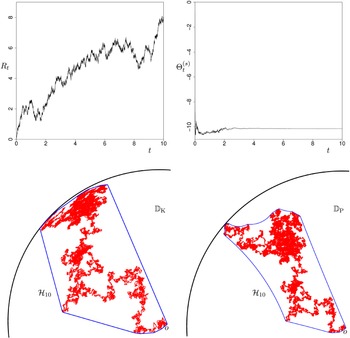
 106
106 Θ(s)
Θ(s) s=10−3
 Bt
Bt t∈[0,10]
 DK
DK H10
H10 DP
DP H2
H2
 Open access

