2.1. The base flow

The boundary layer develops on a long length scale, and can be described by introducing the slow variable

(2.4)\begin{equation} x_3=x/R. \end{equation}

The base-flow density $R_B$, velocity field $(U_B, V_B)$, pressure $P_B$ and temperature $T_B$ can be expressed as

(2.5)\begin{equation} (R_B, U_B, V_B, P_B, T_B)=(\bar{R}(x_3,y), \bar{U}(x_3,y), R^{-1}\bar{V}(x_3,y), 1/(\gamma{M^2}), \bar{T}(x_3,y)). \end{equation}

The steady boundary-layer equations admit the similarity solution (Stewartson Reference Stewartson1964)

(2.6a,b)\begin{equation} \bar{U}=F^\prime(\eta),\quad \bar{T}=\bar{T}(\eta), \end{equation}

where $\eta$ is the similarity variable defined, via the Dorodnitsyn–Howarth coordinate transformation, by

(2.7)\begin{equation} \eta=\frac{1}{\sqrt{x_3}}\int_{0}^{y} \bar{R}\,{\rm d} y. \end{equation}

In terms of $\eta$, $F$ and $\bar {T}$, the steady boundary-layer equations reduce to

(2.8)\begin{equation} \left.\begin{gathered} \frac{1}{2}FF^{\prime\prime}+(\bar{K} F^{\prime\prime})^\prime =0, \\ \bar{T}^{\prime\prime}+\frac{PrF+2\bar{K}^\prime}{2\bar{K}}\bar{T}^\prime+Pr(\gamma-1)M^2(F^{\prime\prime})^2 =0, \end{gathered}\right\} \end{equation}

where we have put $\bar {K}(\bar {T})=\bar \mu (\bar {T})/\bar {T}$. For Sutherland's law, $\bar {K}$ is given by

(2.9)\begin{equation} \bar{K}=\frac{1+C_0}{\bar{T}+C_0}\bar{T}^{1/2}, \end{equation}

where $C_0=110.4\,\mathrm {K}/T_\infty$ with $T_\infty$ being the free-stream temperature in Kelvin. The corresponding boundary conditions are

(2.10)\begin{equation} F(0)=F^\prime(0)=0;\quad F^\prime\rightarrow 1 \quad\mbox{as}\ \eta\rightarrow\infty, \end{equation}

and

(2.11)\begin{equation} \bar{T}(0)=\bar{T}_w;\quad \bar{T}\rightarrow 1 \quad\mbox{as}\ \eta\rightarrow\infty, \end{equation}

if the wall is isothermal with a prescribed temperature $\bar {T}_w$.

We consider a perfect gas with ratio of specific heats $\gamma =1.4$ and Prandtl number $Pr=0.72$. The free-stream temperature is taken to be $T_\infty =300\,\mathrm {K}$, and the Mach number $M=6$. The above chosen parameters are representative of flight conditions (Chuvakhov & Fedorov Reference Chuvakhov and Fedorov2016). The base-flow equations (2.8) are solved by using a shooting method based on a fourth-order Runge–Kutta integrator. The streamwise velocity and temperature for various cooling ratios, defined by the wall temperature over the adiabatic wall temperature, are shown in figure 1. In particular, the base-flow quantities with the cooling ratio $r_c=0.427$ ($\bar {T}_w=3$) will be used in the ensuing analysis. As will be shown later, a radiating mode exists only for $r_c$ below a certain value less than unity.

Figure 1.

The profiles of the base-flow streamwise velocity (a) and temperature (b) for different $r_c$.

2.2. Free-stream acoustic waves

Acoustic waves are one type of elementary disturbances in the free stream, where the base flow is uniform. The density, velocity and pressure components of a two-dimensional acoustic wave, ${\epsilon _s}(\tilde {r}_s, \tilde {u}_s, \tilde {v}_s, \tilde {p}_s)$, where $\epsilon _s\ll 1$ is the magnitude, are governed by the linearised Euler equations about the uniform background field. Eliminating $\tilde {r}_s$, $\tilde {u}_s$ and $\tilde {v}_s$ from these equations leads to the equation for pressure $\tilde {p}_s$

(2.12)\begin{equation} M^2\left(\frac{\partial}{\partial{t}}+\frac{\partial}{\partial{x}}\right)^2\tilde{p}_s-\nabla^2\tilde{p}_s=0. \end{equation}

The solution takes the form

(2.13)\begin{equation} \tilde{p}_s=p_I\exp({\mathrm{i}(\alpha_{s}{x}+\gamma_{s}{y}-\omega_{s}{t})})+\mathrm{c.c.}, \end{equation}

where $\alpha _{s}$ and $\gamma _{s}$ are the streamwise and normal wavenumbers, respectively, and $\omega _{s}$ is the frequency; here, $\gamma _{s}$ is taken to be positive so that the group velocity in the wall-normal direction is negative, i.e. the disturbance represents an incoming wave.

Substitution of (2.13) into (2.12) yields the dispersion relation for slow acoustic waves

(2.14)\begin{equation} c_s\equiv\omega_{s}/\alpha_{s}=1-\frac{1}{M}\sqrt{1+(\gamma_{s}/\alpha_{s})^2}, \end{equation}

where $c_s$ is the phase velocity. We define an incident angle $\theta _s$ by $\cos \theta _s=\alpha _{s}/\sqrt {\alpha _{s}^2+\gamma _{s}^2}$. Use of the dispersion relation (2.14) shows that

(2.15)\begin{equation} \theta_s=\arccos\{1/[(1-c_s)M]\}. \end{equation}

A sound wave in the free stream is characterised by its frequency and incident angle.

2.3. Asymptotic scaling

We are interested in slow acoustic waves and instability modes whose wavelengths are comparable to the boundary-layer thickness (i.e. $\alpha _{s}=O(1)$). Only slow acoustic waves are considered as they have a critical layer, which is crucial for acoustic waves of moderate amplitude to be able to impact the radiating mode. When such a slow acoustic wave impinges on the boundary layer, the response of the latter is in the form of an absorbed disturbance and a reflected wave. For a sound wave with a particular frequency and a specific incident angle, the reflection coefficient becomes infinite, indicating a fundamental resonance between the impinging sound and the intrinsic radiating mode, through which the latter is excited and its evolution influenced. We will investigate these in the non-equilibrium parallel and equilibrium non-parallel regimes.

2.3.1. Non-equilibrium parallel regime

As an inviscid Rayleigh instability mode propagates downstream, its magnitude amplifies exponentially until it reaches a neutral position, $x_{3,n}$ say. Due to the accumulated growth, the mode is likely to enter a nonlinear stage in the vicinity of the neutral position (Goldstein & Leib Reference Goldstein and Leib1989; Wu Reference Wu2019). This region is represented as

(2.16)\begin{equation} x_3\approx x_{3,n}+\tilde\mu\bar{x}_1, \end{equation}

where $\tilde \mu \ll 1$ and $\bar {x}_1=O(1)$ is negative. The local base-flow velocity and temperature profiles are expanded as

(2.17)\begin{equation} (\bar{U}(x_3, y), \bar{T}(x_3, y)) \approx (\bar{U}(x_{3,n}, y), \bar{T}(x_{3,n}, y)) +\tilde\mu(\bar{U}_1(y), \bar{T}_1(y))\bar{x}_1. \end{equation}

In this region, the growth rate of the mode is $O(\tilde \mu )$, correspondingly, the amplitude develops over the length scale of $O(\tilde {\mu }^{-1})$, and so we introduce the slow variable

(2.18)\begin{equation} \tilde{x}=\tilde\mu(x-x_0) \quad\mbox{with}\ x_0=R(x_{3,n}+\tilde\mu\bar{x}_1). \end{equation}

The instability mode is of the travelling-wave form, and in the main layer it can be expressed, to leading order, as

(2.19)\begin{equation} (\tilde\rho, \tilde{u}, \tilde{v}, \tilde{p}, \tilde\theta)=A(\tilde{x}) (\hat{\rho}_0(y), \hat{u}_0(y), \hat{v}_0(y), \hat{p}_0(y), \hat{\theta}_0(y))E+\mathrm{c.c.}+\cdots, \end{equation}

where $E=\exp ({\mathrm {i}\alpha \zeta })$, $\zeta =x-ct$ is the coordinate moving at the phase speed, with $\alpha$ and $c$ being the streamwise wavenumber and phase speed, respectively, and $A(\tilde {x})$ is the amplitude function describing the evolution. The derivative with respect to $x$ then becomes

(2.20)\begin{equation} \frac{\partial}{\partial{x}} \rightarrow \frac{\partial}{\partial\zeta}+\tilde\mu\frac{\partial}{\partial\tilde{x}}. \end{equation}

In order to derive the scaling, let us first write down the streamwise momentum equation (of the incompressible N-S equations for convenience) for the perturbation

(2.21) \begin{align} & \Big[(\bar{U}-c)\frac{\partial}{\partial\zeta} +\underbrace{\tilde\mu\bar{U}\frac{\partial}{\partial\tilde{x}}\Big]\tilde{u}}_{non\text{-}equilibrium} \nonumber\\ &\quad +\bar{U}^\prime\tilde{v}-\underbrace{R^{-1}\frac{\partial^2\tilde{u}}{\partial\tilde{y}^2}}_{{viscous}} =-\frac{\partial\tilde{p}}{\partial\zeta} -\tilde{u}\frac{\partial\tilde{u}}{\partial\zeta}-\tilde{v}\frac{\partial\tilde{u}}{\partial y} -\tilde\mu\tilde{u}\frac{\partial\tilde{u}}{\partial\tilde{x}}+\cdots. \end{align}

The scaling is fixed by considering the main and critical layers. In the main layer, the disturbance is linear and inviscid, and its streamwise velocity exhibits a jump of $O(\tilde {\epsilon }\tilde \mu )$, which is to be determined by analysis of the critical layer. Suppose that the critical-layer width is $O(\delta _c)$. The advection term in (2.21) is $O(\delta _c)$, whereas the terms associated with the non-equilibrium and viscous effects are $O(\tilde \mu )$ and $O(R^{-1}/\delta _c^2)$, respectively. The requirement that these terms are all balanced leads to

(2.22a,b)\begin{equation} \delta_c=O(\tilde\mu),\quad \delta_c=O(R^{-1/3}). \end{equation}

In the critical layer, the vertical velocity of the perturbation $\tilde {v}$ is $O(\tilde {\epsilon })$, but the logarithmic singularity $\ln (y-y_c)$ of the inviscid solution for the streamwise velocity suggests that the vorticity, or $\tilde {u}_y$, is $O(\tilde {\epsilon }\delta _c^{-1})$. The forcing proportional to the product of these two is thus $O(\tilde {\epsilon }^2\delta _c^{-1})$. It then induces a mean-flow distortion as well as a second harmonic; their streamwise velocity is $O(\tilde {\epsilon }^2\delta _c^{-2})$ as is deduced by balancing the forcing and the non-equilibrium term in (2.21). The fundamental wave interacts with them to produce a forcing of $O(\tilde {\epsilon }^3\delta _c^{-3})$ at cubic level, which regenerates an $O(\tilde {\epsilon }^3\delta _c^{-4})$ streamwise velocity of the fundamental. If the latter is comparable to the $O(\tilde {\epsilon }\tilde \mu )$ jump in the main layer, i.e. if $\tilde \mu =O(\tilde {\epsilon }^{2/5})$, the nonlinear effect enters the amplitude equation (Leib Reference Leib1991; Wu & Cowley Reference Wu and Cowley1995). Under this scaling the temperature fluctuation also contributes a nonlinear effect (Goldstein & Leib Reference Goldstein and Leib1989). Due to the resonant nature of the forcing, the $O(\tilde \epsilon )$ radiating mode can be excited by a much weaker incident wave with the magnitude

(2.23)\begin{equation} \tilde{\epsilon}_s=\tilde{\epsilon}\tilde\mu=O(\tilde{\epsilon}^{7/5}). \end{equation}

We then write

(2.24a,b)\begin{equation} \tilde\mu=\tilde{\epsilon}^{2/5}=\delta_c,\quad R^{-1}=\lambda\tilde\mu^3, \end{equation}

where $\lambda$ is the $O(1)$ Haberman parameter measuring the importance of the viscosity. The above relations form the basis of non-equilibrium critical-layer theory describing the interaction between the incident sound and the radiating mode.

2.3.2. Equilibrium non-parallel regime

The equilibrium non-parallel regime is pertinent to the region where the length scale over which the growth rate varies is comparable to the length scale over which the amplitude evolves (Wu Reference Wu2005). This region is represented by

(2.25)\begin{equation} x_3=x_{3,n}+R^{-1/2}\bar{x} \quad\mbox{with}\ \bar{x}=O(1). \end{equation}

We take $\delta ^*$ to be the boundary-layer thickness at the neutral position, and with the latter being chosen to be origin of the coordinate we can set $x_{3,n}=0$. Inspection of (2.21) shows that in this region the non-equilibrium effect, $\bar \mu =O(R^{-1/2})$, is much smaller than the viscous effect. The critical layer is thus of equilibrium type and viscosity dominated, having a width 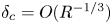$\delta _c=O(R^{-1/3})$. A similar scaling argument shows that the balance between the outer and inner jumps leads to

(2.26)\begin{equation} \bar{\epsilon}=\delta_c^2\bar\mu^{1/2}=O(R^{-11/12}). \end{equation}

Again noting the resonant nature of the forcing, we can infer that the radiating mode of $O(\bar \epsilon )$ can be excited by an incident sound wave with a much smaller magnitude

(2.27)\begin{equation} \bar{\epsilon}_s=O(\bar{\epsilon}\bar\mu)=O(R^{-17/12}). \end{equation}

The local mean velocity and temperature profiles can be approximated by

(2.28)\begin{equation} (\bar{U}(x_3, y), \bar{T}(x_3, y)) \approx (\bar{U}(x_{3,n}, y), \bar{T}(x_{3,n}, y)) +R^{-1/2}(\bar{U}_1(y), \bar{T}_1(y))\bar{x}, \end{equation}

to the required order. With the key scalings identified, the effects of sound waves on the evolution of the radiating mode will be analysed in a self-consistent manner.

2.4. Existence of the radiating mode

For inviscid instability, the linearised Euler equations for instability modes can be reduced to the Rayleigh equation for the pressure

(2.29)\begin{equation} \mathscr{L}\hat{p}_0\equiv\left\{\frac{\partial^2}{\partial y^2} +\left( \frac{\bar{T}^\prime}{\bar{T}}-\frac{2\bar{U}^\prime}{\bar{U}-c} \right)\frac{\partial}{\partial y} -\alpha^2\left[ 1-\frac{M^2(\bar{U}-c)^2}{\bar{T}} \right] \right\}\hat{p}_0=0. \end{equation}

For a neutral radiating mode, the boundary condition consists of the impermeability condition at the wall and a finite amplitude at the infinity, namely, $\hat {p}_0^\prime (0)=0$ and $\hat {p}_0$ is bounded as $y\rightarrow \infty$.

In order to find eigenvalues of the Rayleigh equation, it is convenient to write equation (2.29) in terms of the similarity valuable $\eta$ defined by (2.7) (in which $x_3=x_{3,n}=1$). The Rayleigh equation (2.29) becomes

(2.30)\begin{equation} \hat{p}_0^{\prime\prime}-\frac{2\bar{U}^\prime}{\bar{U}-c}\hat{p}_0^{\prime} -\alpha^2\bar{T}^2\left[1-\frac{M^2(\bar{U}-c)^2}{\bar{T}}\right]\hat{p}_0=0, \end{equation}

where the derivative is with respect to $\eta$, and the boundary condition becomes

(2.31)\begin{equation} \hat{p}_0^\prime(0)=0,\quad \hat{p}_0\ \mbox{is bounded}\quad\mbox{as}\ \eta\rightarrow\infty. \end{equation}

More precisely, the wavenumber and phase velocity of the eigenmode must satisfy the condition, $\alpha ^2[1-M^2(1-c)^2]<0$, or equivalently, $c<1-1/M$, so that the far-field behaviour of the mode takes the form of an outgoing wave

(2.32)\begin{equation} \hat{p}_0\sim \mathscr{C}_{\infty}\exp({-\mathrm{i}\alpha q\eta})\quad\mbox{as}\ \eta\rightarrow\infty, \end{equation}

where $\mathscr {C}_{\infty }$ is the normalisation factor, and $q=\sqrt {M^2(1-c)^2-1}$.

Near the critical level $\eta _c$, where $\bar {U}(\eta _c)-c=0$, we seek solutions of Frobenius type to the Rayleigh equation. It can be shown that, as $\bar {\eta }\equiv \eta -\eta _c\rightarrow 0$,

(2.33)\begin{equation} \hat{p}_0={\bar a}^\pm \bar\phi_a+\bar\phi_b, \end{equation}

where the constants ${\bar a}^\pm$ take different values above and below the critical level, and

(2.34)\begin{gather} \bar\phi_a=\bar{\eta}^3+\frac{3}{4}\frac{\bar{U}_c^{\prime\prime}}{\bar{U}_c^\prime}\bar{\eta}^4+\frac{1}{10} \left[\frac{2\bar{U}_c^{\prime\prime\prime}}{\bar{U}_c^\prime}+\frac{3}{2}\left(\frac{\bar{U}_c^{\prime\prime}}{\bar{U}_c^\prime}\right)^2 +\alpha^2\bar{T}_c^2\right]\bar{\eta}^5+\cdots, \end{gather}

(2.35)\begin{gather}\bar\phi_b=\frac{\alpha^2\bar{T}_c^2}{3} \left(\frac{2\bar{T}_c^\prime}{\bar{T}_c}-\frac{\bar{U}_c^{\prime\prime}}{\bar{U}_c^\prime}\right)\ln|\bar{\eta}|\bar\phi_a +1-\frac{\alpha^2}{2}\bar{T}_c^2\bar{\eta}^2+\bar\chi\bar{\eta}^4+\cdots, \end{gather}

with

(2.36)\begin{align} \bar\chi &= \frac{\alpha^2\bar{T}_c^2}{4}\left[\frac{1}{2}\left(\frac{\bar{U}_c^{\prime\prime}}{\bar{U}_c^\prime} \right)^2 -\frac{2}{3}\frac{\bar{U}_c^{\prime\prime\prime}}{\bar{U}_c^\prime}-\frac{\alpha^2}{2}\bar{T}_c^2 +\frac{\bar{T}_c^{\prime\prime}}{\bar{T}_c}+\left( \frac{\bar{T}_c^\prime}{\bar{T}_c} \right)^2\right] \nonumber\\ &\quad -\frac{M^2\alpha^2}{4}(\bar{U}_c^\prime)^2\bar{T}_c-\frac{11}{48}\alpha^2\bar{T}_c^2\frac{\bar{U}_c^{\prime\prime}}{\bar{U}_c^\prime} \left(\frac{2\bar{T}_c^\prime}{\bar{T}_c}-\frac{\bar{U}_c^{\prime\prime}}{\bar{U}_c^\prime}\right). \end{align}

The analytical formula above supplements the numerical method to solve the eigenvalue problem, the details of which are relegated to Appendix A.1.

For the base-flow condition considered, we find a radiating mode with

(2.37a,b)\begin{equation} \alpha=0.355336,\quad c=0.723147, \end{equation}

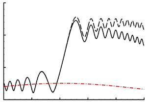
and plot the corresponding eigenfunction in figure 2. As is shown, the radiating (supersonic) mode exhibits a wavy structure in the far field, in contrast to the subsonic mode which decays exponentially outside the boundary layer. This feature is closely related to the Mach wave radiation (Wu Reference Wu2005). The dependence of the radiating mode on the base-flow parameters is studied. The variation of the streamwise wavenumber and phase velocity of the neutral radiating mode with the Mach number $M$ for a fixed wall temperature $\bar {T}_w=3$ is shown in figure 3. A radiating mode exists only in a small range of Mach number. Similarly, for a fixed Mach number ($M=6$), a radiating mode could only be found in a small range of the cooling ratio, as is shown in figure 4.

Figure 2.

The eigenfunction of a two-dimensional supersonic mode: (a) $\hat {p}_0$ and (b) $\hat {p}_0^{\prime }$.

Figure 3.

Variation of the wavenumber $\alpha$ (a) and the phase speed $c$ (b) of the neutral radiating mode with the Mach number $M$ for a fixed wall temperature $\bar {T}_w=3$ ($r_c=0.427$).

Figure 4.

Variation of the wavenumber $\alpha$ (a) and the phase speed $c$ (b) of the neutral radiating mode with the cooling ratio $r_c$ for a fixed Mach number $M=6$.

3.1. Main layer

In the main layer, where $y=O(1)$, the disturbance expands as

(3.1)\begin{align} (\tilde\rho, \tilde{u}, \tilde{v}, \tilde{p}, \tilde\theta)=\epsilon_s (\check\rho_s(x_3,y), \check{u}_s(x_3,y), \check{v}_s(x_3,y), \check{p}_s(x_3,y), \check\theta_s(x_3,y))E_s+\mathrm{c.c.}+\cdots, \end{align}

where $E_s=\exp ({\mathrm {i}\alpha _{s}(x-c_s t)})$, and the dependence on $x_3$ is parametric. Substitution of (3.1) into (2.2) followed by linearisation yields the equations

(3.2a)\begin{gather} \mathrm{i}\alpha_{s}(\bar{U}-c_s)\check\rho_s+\bar{R}^\prime \check{v}_s+\bar{R}(\mathrm{i}\alpha_{s} \check{u}_s+\check{v}_{s,y})=0, \end{gather}

(3.2b)\begin{gather}\mathrm{i}\alpha_{s}(\bar{U}-c_s)\check{u}_s+\bar{U}^\prime \check{v}_s=-\mathrm{i}\alpha_{s}\bar{T} \check{p}_s, \end{gather}

(3.2c)\begin{gather}\mathrm{i}\alpha_{s}(\bar{U}-c_s)\check{v}_s=-\bar{T} \check{p}_{s,y}, \end{gather}

(3.2d)\begin{gather}\mathrm{i}\alpha_{s}(\bar{U}-c_s)\check\theta_s+\bar{T}^\prime \check{v}_s =\mathrm{i}\alpha_{s}(\gamma-1)M^2(\bar{U}-c_s)\bar{T} \check{p}_s, \end{gather}

(3.2e)\begin{gather}\gamma M^2 \check{p}_s=\bar{R}\check\theta_s+\bar{T}\check\rho_s, \end{gather}

where the prime ‘$\prime$’ in the base-flow quantities denotes the partial differentiation with respect to $y$. Elimination of $\check \rho _s$, $\check {u}_s$, $\check {v}_s$ and $\check \theta _s$ leads to the compressible Rayleigh equation for pressure $\check {p}_s$

(3.3)\begin{equation} \check{p}_{s,yy}+\left( \frac{\bar{T}^\prime}{\bar{T}}-\frac{2\bar{U}^\prime}{\bar{U}-c_s} \right)\check{p}_{s,y} -\alpha_{s}^2\left[ 1-\frac{M^2(\bar{U}-c_s)^2}{\bar{T}} \right]\check{p}_s=0. \end{equation}

The above equation must be solved subject to the impermeability condition, $\check {p}_{s,y}(0)=0$, as implied by (3.2c). In the far field, the pressure takes the form

(3.4)\begin{equation} \check{p}_s\sim p_I[\exp({\mathrm{i}\gamma_{s} y})+\mathscr{R}(x_3)\exp({-\mathrm{i}\gamma_{s} y})] \quad\mbox{as}\ y\rightarrow\infty, \end{equation}

which represents an incident wave and a reflected wave; here, $\gamma _{s}=\alpha _{s}\sqrt {M^2(1-c_s)^2-1}$, and $\mathscr {R}$ is the reflection coefficient. The solution exhibits a singularity at the critical level $y_c(x_3)$, at which $\bar {U}(x_3, y_c)=c_s$. As $\tilde \eta \equiv y-y_c\rightarrow 0$, the local solution to (3.3) is constructed by using the Frobenius method as

(3.5)\begin{equation} \check{p}_s=a_s^\pm(x_3)\phi_{sa}+b_s^\pm(x_3)\left[\phi_{sb} +\frac{\alpha_{s}^2}{3}\left(\frac{\bar{T}_c^\prime}{\bar{T}_c}- \frac{\bar{U}_c^{\prime\prime}}{\bar{U}_c^\prime}\right)\ln|\tilde\eta|\phi_{sa}\right], \end{equation}

where

(3.6)\begin{align} \phi_{sa} &=\tilde\eta^3+\chi_{sa}\tilde\eta^4 +\frac{1}{10}\left[3\left(\frac{\bar{T}_c^\prime}{\bar{T}_c}-\frac{\bar{U}_c^{\prime\prime}}{\bar{U}_c^\prime}\right)^2 -\frac{3}{2}\left(\frac{\bar{U}_c^{\prime\prime}}{\bar{U}_c^\prime} \right)^2 \right. \nonumber\\ &\quad + \left.\frac{2\bar{U}_c^{\prime\prime\prime}}{\bar{U}_c^\prime} -\frac{3\bar{T}_c^{\prime\prime}}{\bar{T}_c}+3\left(\frac{\bar{T}_c^\prime}{\bar{T}_c}\right)^2+\alpha_{s}^2\right]\tilde\eta^5+\cdots, \end{align}

(3.7)\begin{equation} \phi_{sb}=1-\frac{\alpha_{s}^2}{2}\tilde\eta^2+\chi_{sb}\tilde\eta^4+\cdots, \end{equation}

with

(3.8)\begin{gather} \chi_{sa}=-\frac{3}{4}\left( \frac{\bar{T}_c^\prime}{\bar{T}_c}-\frac{\bar{U}_c^{\prime\prime}}{\bar{U}_c^\prime} \right), \end{gather}

(3.9)\begin{gather}\chi_{sb}=\frac{\alpha_{s}^2}{4}\left[ \frac{\bar{T}_c^{\prime\prime}}{\bar{T}_c}-\left( \frac{\bar{T}_c^\prime}{\bar{T}_c} \right)^2 +\frac{1}{2}\left( \frac{\bar{U}_c^{\prime\prime}}{\bar{U}_c^\prime} \right)^2 -\frac{2}{3}\frac{\bar{U}_c^{\prime\prime\prime}}{\bar{U}_c^\prime}-\frac{M^2(\bar{U}_c^\prime)^2}{\bar{T}_c} -\frac{\alpha_{s}^2}{2}+\frac{11}{12}\left( \frac{\bar{T}_c^\prime}{\bar{T}_c}-\frac{\bar{U}_c^{\prime\prime}}{\bar{U}_c^\prime}\right)^2\right]. \end{gather}

The pressure, velocities and temperature of the disturbance have the expressions

(3.10a)\begin{equation} \check{p}_s=b_s^\pm\left[ 1-\frac{\alpha_{s}^2}{2}\tilde\eta^2+\frac{\alpha_{s}^2}{3} \left(\frac{\bar{T}_c^\prime}{\bar{T}_c}-\frac{\bar{U}_c^{\prime\prime}}{\bar{U}_c^\prime} \right)\tilde\eta^3\ln|\tilde\eta| +(a_s^\pm{/}b_s^\pm)\tilde\eta^3 \right]+O(\tilde\eta^4\ln|\tilde\eta|), \end{equation}

(3.10b)\begin{align} \check{v}_s &=-\mathrm{i}\alpha_{s} b_s^\pm\frac{\bar{T}_c}{\bar{U}_c^\prime}\left[ 1- \left(\frac{\bar{T}_c^\prime}{\bar{T}_c}-\frac{\bar{U}_c^{\prime\prime}}{\bar{U}_c^\prime} \right)\tilde\eta\ln|\tilde\eta| \right.\nonumber\\ &\quad \left.+\left(\frac{2}{3}\frac{\bar{T}_c^\prime}{\bar{T}_c}-\frac{1}{6}\frac{\bar{U}_c^{\prime\prime}}{\bar{U}_c^\prime} -\frac{3a_s^\pm}{\alpha_{s}^2b_s^\pm} \right)\tilde\eta \right]+O(\tilde\eta^2\ln|\tilde\eta|), \end{align}

(3.10c)\begin{gather} \check{u}_s=b_s^\pm\frac{\bar{T}_c}{\bar{U}_c^\prime}\left[-\left(\frac{\bar{T}_c^\prime}{\bar{T}_c}-\frac{\bar{U}_c^{\prime\prime}}{\bar{U}_c^\prime} \right)\ln|\tilde\eta| +\frac{5}{6}\frac{\bar{U}_c^{\prime\prime}}{\bar{U}_c^\prime}-\frac{1}{3}\frac{\bar{T}_c^\prime}{\bar{T}_c} -\frac{3a_s^\pm}{\alpha_{s}^2 b_s^\pm} \right]+O(\tilde\eta\ln|\tilde\eta|), \end{gather}

(3.10d)\begin{gather}\check\theta_s=b_s^\pm\frac{\bar{T}_c\bar{T}_c^\prime}{(\bar{U}_c^\prime)^2}\left[ \frac{1}{\tilde\eta} -\left(\frac{\bar{T}_c^\prime}{\bar{T}_c}-\frac{\bar{U}_c^{\prime\prime}}{\bar{U}_c^\prime} \right)\ln|\tilde\eta| \right]+O(1). \end{gather}

Clearly, the temperature perturbation $\check \theta _s$ has a simple-pole singularity, while the streamwise velocity $\check {u}_s$ exhibits a logarithmic singularity, indicating that the main-layer solution breaks down as $\tilde \eta \rightarrow 0$. Thus we need to analyse the critical layer.

3.2. Critical layer

By balancing the advection and viscous terms in the momentum or energy equation, we find the critical-layer thickness $\delta =O(R^{-1/3})$. Then taking $\delta =R^{-1/3}$, we introduce an inner variable

(3.11)\begin{equation} Y=(y-y_c)/\delta. \end{equation}

In view of the inner limit of the outer expansion (3.10a)–(3.10d), the inner expansion takes the form

(3.12a)\begin{gather} \tilde{u}=\epsilon_s(\ln\delta U_{sl0}+U_{s1}+\cdots)E_s+\mathrm{c.c.}, \end{gather}

(3.12b)\begin{gather}\tilde{v}=\epsilon_s(V_{s0}+\delta\ln\delta V_{sl0}+\delta V_{s1}+\cdots)E_s+\mathrm{c.c.}, \end{gather}

(3.12c)\begin{gather}\tilde{p}=\epsilon_s(P_{s0}+\delta^2 P_{s1}+\delta^3\ln\delta P_{sl1}+\cdots)E_s+\mathrm{c.c.}, \end{gather}

(3.12d)\begin{gather}\tilde\theta=\epsilon_s(\delta^{-1}\varTheta_{s0}+\ln\delta \varTheta_{sl0}+\varTheta_{s1}+\cdots)E_s+\mathrm{c.c.} . \end{gather}

At leading order, the $y$-momentum equation gives $P_{s0,Y}=0$, which implies $P_{s0}=P_{s0}(x_3)$. Matching with the main-layer solution leads to

(3.13)\begin{equation} b_s^+=P_{s0}=b_s^-\equiv b_s. \end{equation}

The continuity, $x$-momentum and energy equations for the leading-order terms read $V_{s0,Y}=0$, and

(3.14a)\begin{gather} \bar{U}_c^\prime V_{s0}=-\mathrm{i}\alpha_{s}\bar{T}_c P_{s0}, \end{gather}

(3.14b)\begin{gather}\mathrm{i}\alpha_{s}\bar{U}_c^\prime Y \varTheta_{s0}+\bar{T}_c^\prime V_{s0}=\bar{T}_c\bar{\mu}_c Pr^{-1}\varTheta_{s0,YY}, \end{gather}

respectively. The solution is found to be

(3.15a)\begin{gather} V_{s0}=-\mathrm{i}\alpha_{s} b_s\bar{T}_c/\bar{U}_c^\prime, \end{gather}

(3.15b)\begin{gather}\varTheta_{s0}=\mathrm{i}\alpha_{s}\frac{\bar{T}_c\bar{T}_c^\prime}{\bar{U}_c^\prime}b_s\! \int_{0}^{\infty} \!\exp(-s_{sp}\xi^3-\mathrm{i}\alpha_{s}\bar{U}_c^\prime Y\xi)\,{\rm d}\xi \quad\mbox{with}\ s_{sp}={\textstyle\frac{1}{3}}(\alpha_{s}\bar{U}_c^\prime)^2\bar{T}_c\bar{\mu}_c Pr^{-1}. \end{gather}

It is found that the logarithm terms match their counterparts in the outer solution automatically. At the next order, the continuity and $x$-momentum equations yield

(3.16a)\begin{gather} \mathrm{i}\alpha_{s}\bar{U}_c^\prime Y(-\varTheta_{s0}/\bar{T}_c^2) +(\mathrm{i}\alpha_{s} U_{s1}+V_{s1,Y})/\bar{T}_c -(\bar{T}_c^\prime/\bar{T}_c^2)V_{s0}=0, \end{gather}

(3.16b)\begin{gather}\mathscr{L}_s U_{s1}+\bar{U}_c^\prime V_{s1}+\bar{U}_c^{\prime\prime} Y V_{s0} =-\mathrm{i}\alpha_{s}\bar{T}_c^\prime Y P_{s0}+\bar{T}_c\bar{U}_c^\prime\bar{\mu}_c^\prime\varTheta_{s0,Y}, \end{gather}

where $\bar {\mu }_c^\prime =(\textrm {d}\bar \mu /\textrm {d}\bar {T})|_{y=y_c}$, and the operator $\mathscr {L}_s$ is defined by

(3.17)\begin{equation} \mathscr{L}_s=\mathrm{i}\alpha_{s}\bar{U}_c^\prime Y-\bar{T}_c\bar{\mu}_c\frac{\partial^2}{\partial Y^2}. \end{equation}

Eliminating $V_{s1}$ in the above two equations, and solving the resulting equation, the solution is found to be

(3.18)\begin{align} U_{s1,Y} &= \mathrm{i}\alpha_{s}\frac{\bar{T}_c^\prime(\bar{T}_c\bar{\mu}_c^\prime-\bar{\mu}_c Pr^{-1})}{\bar{\mu}_c(1-Pr^{-1})}b_s\! \int_{0}^{\infty}\! [1-\exp(-(s_{sp}-s_s)\xi^3)]\nonumber\\ &\quad \times\exp(-s_s\xi^3-\mathrm{i}\alpha_{s}\bar{U}_c^\prime Y\xi)\,{\rm d}\xi \nonumber\\ &\quad -\mathrm{i}\alpha_{s}\bar{T}_c\left(\frac{\bar{T}_c^\prime}{\bar{T}_c}-\frac{\bar{U}_c^{\prime\prime}}{\bar{U}_c^\prime} \right)b_s\! \int_{0}^{\infty} \!\exp(-s_s\xi^3-\mathrm{i}\alpha_{s}\bar{U}_c^\prime Y\xi)\,{\rm d}\xi, \end{align}

where $s_s={\frac {1}{3}}(\alpha _{s}\bar {U}_c^\prime )^2\bar {T}_c\bar {\mu }_c$. Matching $U_{s1}$ with its outer counterpart (3.10c) determines the jump

(3.19)\begin{equation} a_s^+- a_s^-= \frac{\alpha_{s}^2}{3}\left(\frac{\bar{T}_c^\prime}{\bar{T}_c}-\frac{\bar{U}_c^{\prime\prime}}{\bar{U}_c^\prime} \right)b_s{\rm \pi}\mathrm{i}. \end{equation}

This jump is used together with the numerical method to obtain the reflection coefficient and boundary-layer response; the details are described in Appendix A.2.

3.3. The reflection coefficient and boundary-layer response

For each incident wave, we compute $\mathscr {R}$ and $\tilde {b}$, where $\tilde {b}$, introduced in (A16) as the ratio of the pressure amplitude in the critical layer to the amplitude of the incident wave, is a measure of the boundary-layer response. For the particular incident wave satisfying the resonant condition, $(\alpha _{s},c_s)=(0.355,0.723)$, it is found that $\mathscr {R}=1.299\times 10^{7}+5.140\times 10^{7}\mathrm {i}$ and $\tilde {b}=5.725\times 10^{7}-7.032\times 10^{6}\mathrm {i}$. They are numerically large, indeed practically infinite, indicating that the resonant over-reflection coincides with the onset of a neutral radiating mode.

Recalling that $\omega _s=\alpha _{s} c_s$ and (2.15), we can regard $|\mathscr {R}|$ and $|\tilde {b}|$ as functions of $\theta _s$ and $\omega _s$. Figure 6(a,b) shows contours of $|\mathscr {R}|$ and $|\tilde {b}|$ in the $\theta _s$–$\omega _s$ plane with increments ${\rm \Delta} \theta _s=0.1$ and ${\rm \Delta} \omega _s=10^{-3}$. For most frequencies and incident angles, the boundary-layer response $|\tilde {b}|$ is finite and indeed rather small, while the reflection coefficient remains almost unchanged around the value of unity, indicating that these reflected acoustic waves have roughly the same magnitude as that of incident ones, and the boundary layer does not play a role in the reflection process. A prominent feature is that there appear two long strips indicating a very steep gradient, one of which passes through the resonant point (52.987, 0.257), where the response becomes infinite. The reflection coefficient increases rapidly when approaching either of the two strips. To show further details of the strips, we compute contours of two small regions in the lower strip using a smaller increment, and the results are displayed in figure 6(c,e). The reflection coefficient soars to very large values for a narrow frequency band, resulting in elongated contours enclosing the resonant point. Strong over-reflection occurs for $(\theta _s,\omega _s)$ in the strips. Similarly, $|\tilde {b}|$ acquires large values in the strips, as is shown by figure 6(b) and the enlarged views of the two selected zones (figure 6d,f). These imply that the incident wave facilitates transfer of a considerable amount of energy from the shear flow while the reflected wave absorbs a significant amount from it.

Figure 6.

Contours of $|\mathscr {R}|$ (a) and $|\tilde {b}|$ (b) in the $\theta _s$–$\omega _s$ plane. The resonant point is located at (52.987, 0.257). (c,d) Zoom into the range $39<\theta _s<41$. (e,f) Zoom into the range $61.2<\theta _s<61.6$.

To show further the dependence of the boundary-layer response on the parameters, we plot the variations of the reflection coefficient $|\mathscr {R}|$ and response $|\tilde {b}|$ with frequency $\omega _s$ at different incident angles. Figure 7(a,b) depicts the variations of $|\mathscr {R}|$ and $|\tilde {b}|$ with $\omega _s$ at $\theta _s=40^{\circ }$, respectively. Two sharp peaks appear at $\omega _s=0.233$ and $0.614$, which lie in the strips in the contours. In order to determine the nature of these peak values, calculations of the variations near the peaks are performed. The panels in figure 7(a,b) zoom into the range near $\omega _s=0.233$ and $0.614$. The sharp peaks turn out to be finite in these ranges. The peak values in the upper strip (the zoomed views near $\omega _s=0.614$) are markedly smaller than those in the lower strip (the zoomed views near $\omega _s=0.233$). Notably, the frequency range over which the peak varies in the upper strip is of $O(10^{-4})$, which is much smaller than $O(10^{-3})$ in the lower strip. Figure 7(c,d) plots the variations of $|\mathscr {R}|$ and $|\tilde {b}|$ with $\omega _s$ at $\theta _s=52.987^{\circ }$, which is the resonant angle. Two sharp peaks at $\omega _s=0.257$ and $0.702$ are observed. As $\omega _s$ approaches $0.257$ (the resonant frequency), $|\mathscr {R}|$ and $|\tilde {b}|$ become unbounded as is shown by enlarged views near $\omega _s=0.257$, signalling the onset of resonance, while the zoomed views near $\omega _s=0.702$ show the abrupt rise of $|\mathscr {R}|$ and $|\tilde {b}|$ to their peak values in the upper strip. Figure 7(e,f) shows the variations of $|\mathscr {R}|$ and $|\tilde {b}|$ with $\omega _s$ at $\theta _s=61.4^{\circ }$. The patterns resemble those at $\theta _s=40^{\circ }$.

Figure 7.

Variations of $|\mathscr {R}|$ and $|\tilde {b}|$ with $\omega _{s}$ at $\theta _s=40^{\circ }$ (a,b), $52.987^{\circ }$ (c,d) and $61.4^{\circ }$ (e,f).

4.1. Non-equilibrium parallel regime

The scaling argument in § 2.3.1 shows that the radiating mode evolves nonlinearly with the rate $\tilde \mu =\tilde {\epsilon }^{2/5}$ when its amplitude $\tilde \epsilon =O(R^{-5/6})$, and such a mode may be excited and/or affected by the incident sound of a much smaller magnitude $\tilde {\epsilon }_s=\tilde {\epsilon }\tilde \mu =O(R^{-7/6})$ due to resonance. Detuning effects may be included by allowing the wavenumber of the sound to differ from that of the radiating mode by an $O(\tilde \mu )$ amount, that is,

(4.1a,b)\begin{equation} \alpha_{s}=\alpha+\tilde\mu\tilde\alpha_d,\quad \omega_{s}=\omega, \end{equation}

where $\tilde \alpha _d$ is an $O(1)$ detuning parameter.

4.1.1. Main layer

In the main layer, the disturbance expands as

(4.2)\begin{equation} (\tilde\rho, \tilde{u}, \tilde{v}, \tilde{p}, \tilde\theta)= \tilde{\epsilon}_s\tilde\mu^{-1}[\tilde{A}(\tilde{x})(\hat{\rho}_0, \hat{u}_0, \hat{v}_0, \hat{p}_0, \hat{\theta}_0) +\tilde\mu(\hat{\rho}_1, \hat{u}_1, \hat{v}_1, \hat{p}_1, \hat{\theta}_1)]E+\mathrm{c.c.}+\cdots, \end{equation}

where $E=\exp ({\mathrm {i}\alpha (x-ct)})$ is the carrier wave, and the first term represents a radiating mode, which may be locally excited and/or propagates from upstream with $\tilde {A}(\tilde {x})$ being its amplitude function. Substitution of (4.2) into (2.2) followed by linearisation yields the leading-order equations for the disturbance

(4.3a)\begin{gather} \mathrm{i}\alpha(\bar{U}-c)\hat{\rho}_0+\bar{R}^\prime\hat{v}_0+\bar{R}(\mathrm{i}\alpha\hat{u}_0+\hat{v}_0^\prime)=0, \end{gather}

(4.3b)\begin{gather}\mathrm{i}\alpha(\bar{U}-c)\hat{u}_0+\bar{U}^\prime\hat{v}_0=-\mathrm{i}\alpha\bar{T}\hat{p}_0, \end{gather}

(4.3c)\begin{gather}\mathrm{i}\alpha(\bar{U}-c)\hat{v}_0=-\bar{T}\hat{p}_0^\prime, \end{gather}

(4.3d)\begin{gather}\mathrm{i}\alpha(\bar{U}-c)\hat{\theta}_0+\bar{T}^\prime\hat{v}_0 =\mathrm{i}\alpha(\gamma-1)M^2(\bar{U}-c)\bar{T}\hat{p}_0, \end{gather}

(4.3e)\begin{gather}\gamma M^2 \hat{p}_0=\bar{R}\hat{\theta}_0+\bar{T}\hat{\rho}_0. \end{gather}

Elimination of $\hat {\rho }_0$, $\hat {u}_0$, $\hat {v}_0$ and $\hat {\theta }_0$ leads to the familiar compressible Rayleigh equation (2.29) for the leading-order pressure $\hat {p}_0$. As $y\rightarrow \infty$,

(4.4)\begin{equation} \hat{p}_0\sim\mathscr{C}_{\infty}\exp({-\mathrm{i}\alpha q y}) \quad\mbox{with}\ q=\sqrt{M^2(1-c)^2-1}, \end{equation}

which represents an outgoing wave that persists away from the main layer. Here, $\mathscr {C}_{\infty }$ is a constant that is determined by normalisation of the eigenfunction.

Let $\hat {\eta }\equiv y-y_c\rightarrow 0$, the solution near the critical level $y_c$ is obtained using the Frobenius method as

(4.5)\begin{equation} \hat{p}_0\sim\frac{\bar{U}_c^\prime}{\bar{T}_c}\left\{ \frac{\alpha^2}{3}a^{{\pm}}\phi_a+\phi_b +\frac{\alpha^2}{3}\left( \frac{\bar{T}_c^\prime}{\bar{T}_c}-\frac{\bar{U}_c^{\prime\prime}}{\bar{U}_c^\prime} \right)\ln|\hat{\eta}|\phi_a \right\}, \end{equation}

where $\phi _a$ and $\phi _b$ have the same expressions as $\phi _{sa}$ and $\phi _{sb}$ given by (3.6) and (3.7), respectively, with $\alpha$ replacing $\alpha _{s}$. It follows from (4.3b)–(4.3d) that, as $\hat {\eta }\rightarrow 0$,

(4.6)\begin{gather} \hat{u}_0\sim-\left( \frac{\bar{T}_c^\prime}{\bar{T}_c}-\frac{\bar{U}_c^{\prime\prime}}{\bar{U}_c^\prime} \right)\ln|\hat{\eta}| +\frac{5}{6}\frac{\bar{U}_c^{\prime\prime}}{\bar{U}_c^\prime}-\frac{1}{3}\frac{\bar{T}_c^\prime}{\bar{T}_c}-a^{{\pm}}+\cdots, \end{gather}

(4.7)\begin{gather}\hat{v}_0\sim-\mathrm{i}\alpha\left\{1-\left(\frac{\bar{T}_c^\prime}{\bar{T}_c}-\frac{\bar{U}_c^{\prime\prime}}{\bar{U}_c^\prime}\right)\hat{\eta}\ln|\hat{\eta}| +\left(\frac{2}{3}\frac{\bar{T}_c^\prime}{\bar{T}_c}-\frac{1}{6}\frac{\bar{U}_c^{\prime\prime}}{\bar{U}_c^\prime}-a^{{\pm}} \right)\hat{\eta} +\cdots \right\}, \end{gather}

(4.8)\begin{gather}\hat{\theta}_0\sim \frac{\bar{T}_c^\prime}{\bar{U}_c^\prime\hat{\eta}}. \end{gather}

The temperature perturbation exhibits the same simple-pole singularity as that of an inflectional mode (Goldstein & Leib Reference Goldstein and Leib1989), while the logarithmic singularity is present only for a supersonic mode, whose critical level does not correspond to the generalised inflection point (Leib Reference Leib1991). Equation (4.6) indicates a jump of $\hat {u}_0$

(4.9) \begin{equation} \hat{u}_0^+- \hat{u}_0^-= -(a^+- a^-)+\cdots. \end{equation}

At the next order, the second terms in the expansion (4.2), $(\hat {\rho }_1, \hat {u}_1, \hat {v}_1, \hat {p}_1, \hat {\theta }_1)$, are found to satisfy the inhomogeneous version of (4.3a)–(4.3e) (Qin Reference Qin2024). By eliminating $\hat {\rho }_1$, $\hat {u}_1$, $\hat {v}_1$ and $\hat {\theta }_1$ from those equations, we can show that $\hat {p}_1$ satisfies an inhomogeneous Rayleigh equation (Wu Reference Wu2005; Qin Reference Qin2024)

(4.10) \begin{equation} \mathscr{L}\hat{p}_1=\tilde{A}^\prime\frac{2\mathrm{i} c}{\alpha}\biggl\{ \frac{\bar{U}^\prime\hat{p}_0^\prime}{(\bar{U}-c)^2} +\frac{\alpha^2}{c}\left[ \frac{M^2\bar{U}(\bar{U}-c)}{\bar{T}}-1 \right]\hat{p}_0 \biggr\} -\bar{x}_1 \tilde{A}\varDelta_1, \end{equation}

where we have put

(4.11) \begin{align} \varDelta_1 &= \biggl\{\frac{2\bar{U}^\prime}{\bar{U}-c}\biggl(\frac{\bar{U}_1}{\bar{U}-c}- \frac{\bar{U}_1^\prime}{\bar{U}^\prime}\biggr)+\frac{\bar{T}^\prime}{\bar{T}}\biggl( \frac{\bar{T}_1^\prime}{\bar{T}^\prime}- \frac{\bar{T}_1}{\bar{T}} \biggr) \biggr\}\hat{p}_0^\prime \nonumber\\ &\quad +\alpha^2 M^2\frac{(\bar{U}-c)^2}{\bar{T}}\left( \frac{2\bar{U}_1}{\bar{U}-c}-\frac{\bar{T}_1}{\bar{T}} \right)\hat{p}_0. \end{align}

As $y\rightarrow \infty$, the incident acoustic wave must be included in the far-field boundary condition, which reads

(4.12)\begin{align} \hat{p}_1 &\sim p_I\exp({\mathrm{i}\tilde\alpha_d\tilde{x}})[\exp({\mathrm{i}\alpha q y}) +\hat{\mathscr{R}}(\tilde{x})\exp({-\mathrm{i}\alpha q y})] \nonumber\\ &\quad +q^{-1}[1-M^2(1-c)]\mathscr{C}_{\infty}\tilde{A}^\prime y\exp({-\mathrm{i}\alpha q y}). \end{align}

On the other hand, by the method of dominant balance we deduce that, as $y\rightarrow y_c$,

(4.13)\begin{align} \hat{p}_1 &\sim \frac{\alpha^2}{\bar{T}_c}\left( \frac{\mathrm{i} c}{\alpha}\tilde{A}^\prime-\bar{U}_{1c}\bar{x}_1 \tilde{A} \right) \left\{ \hat{\eta}-\left( \frac{\bar{T}_c^\prime}{\bar{T}_c}-\frac{\bar{U}_c^{\prime\prime}}{\bar{U}_c^\prime} \right)\hat{\eta}^2\ln|\hat{\eta}| \right.\nonumber\\ &\quad \left.-\left[ a^{{\pm}}+\frac{1}{3}\left( \frac{\bar{T}_c^\prime}{\bar{T}_c}-\frac{\bar{U}_c^{\prime\prime}}{\bar{U}_c^\prime} \right) \right]\hat{\eta}^2 +\frac{1}{3}j\hat{\eta}^3\ln|\hat{\eta}| \right\}+\frac{\bar{U}_c^\prime}{\bar{T}_c}(\mathrm{i}\alpha \tilde{A}^\prime)\hat{\eta}^2 \nonumber\\ &\quad +\left( \frac{\alpha^2\bar{U}_c^\prime}{3\bar{T}_c}\bar{x}_1 \tilde{A} \right)j_1\hat{\eta}^3\ln|\hat{\eta}| +c^{{\pm}}\phi_a +d\left[ \phi_b+\frac{\alpha^2}{3}\left( \frac{\bar{T}_c^\prime}{\bar{T}_c}-\frac{\bar{U}_c^{\prime\prime}}{\bar{U}_c^\prime} \right)\ln|\hat{\eta}|\phi_a \right], \end{align}

where $c^{\pm }$ and $d$ are arbitrary functions of $\tilde {x}$, and the constants, $j$ and $j_1$, have the expressions

(4.14)\begin{gather} j=\frac{\bar{T}_c^{\prime\prime}}{\bar{T}_c}-\frac{\bar{U}_c^{\prime\prime\prime}}{\bar{U}_c^\prime} -\left(\frac{\bar{T}_c^\prime}{\bar{T}_c} \right)^2 +\left(\frac{\bar{U}_c^{\prime\prime}}{\bar{U}_c^\prime} \right)^2 +3\left(\frac{\bar{T}_c^\prime}{\bar{T}_c}-\frac{\bar{U}_c^{\prime\prime}}{\bar{U}_c^\prime} \right)^2 -2\left(\frac{\bar{T}_c^\prime}{\bar{T}_c}-\frac{\bar{U}_c^{\prime\prime}}{\bar{U}_c^\prime} \right)\frac{\bar{U}_c^\prime}{\bar{U}_c}, \end{gather}

(4.15) \begin{gather} j_1=\frac{\bar{T}_c^\prime}{\bar{T}_c}\biggl(\frac{\bar{T}_{1c}^\prime}{\bar{T}_c^\prime}-\frac{\bar{T}_{1c}}{\bar{T}_c}\biggl) +\frac{\bar{U}_c^{\prime\prime}}{\bar{U}_c^\prime}\biggl(\frac{\bar{U}_{1c}^\prime}{\bar{U}_c^\prime}-\frac{\bar{U}_{1c}^{\prime\prime}}{\bar{U}_c^{\prime\prime}}\biggr) -2\left(\frac{\bar{T}_c^\prime}{\bar{T}_c}-\frac{\bar{U}_c^{\prime\prime}}{\bar{U}_c^\prime} \right)\frac{\bar{U}_{1c}}{\bar{U}_c}. \end{gather}

It follows from the $x$- and $y$-momentum equations that

(4.16)\begin{equation} \hat{u}_1=-\frac{\bar{T}}{\bar{U}-c}\hat{p}_1-\frac{\bar{T}\bar{U}^\prime}{\alpha^2(\bar{U}-c)^2}\hat{p}_{1,y}+\cdots. \end{equation}

Thus, the jump of $\hat {u}_1$ is found to relate to $(c^+ - c^-)$ by the equation

(4.17)\begin{equation} \hat{u}_1^+- \hat{u}_1^-= -\frac{3\bar{T}_c}{\alpha^2\bar{U}_c^\prime}(c^+- c^-)+\cdots. \end{equation}

In order for the inhomogeneous equation (4.10) to have an acceptable solution, it has to satisfy a solvability condition. This can be derived by multiplying both sides of (4.10) by $\hat {p}_0\bar {T}/(\bar {U}-c)^2$ and integrating from $0$ to $\infty$, leading to

(4.18)\begin{equation} -\frac{\bar{T}}{(\bar{U}-c)^2}[(\hat{p}_0\hat{p}_{1,y}-\hat{p}_0^\prime\hat{p}_1) \rvert_{y\rightarrow y_c^-}^{y\rightarrow y_c^+} -(\hat{p}_0\hat{p}_{1,y}-\hat{p}_0^\prime\hat{p}_1)\rvert_{y=\infty}] =\frac{2\mathrm{i} c}{\alpha}I_2 \tilde{A}^\prime-I_1\bar{x}_1 \tilde{A}, \end{equation}

where use has been made of the impermeability condition $\hat {p}_0^\prime (0)=\hat {p}_{1,y}|_{y=0}=0$, and

(4.19) \begin{align} I_1 &= \int_{0}^{\infty} \biggl\{\biggl[\frac{2\bar{U}^\prime}{\bar{U}-c} \biggl(\frac{\bar{U}_1}{\bar{U}-c}-\frac{\bar{U}_1^\prime}{\bar{U}^\prime} \biggr) +\frac{\bar{T}^\prime}{\bar{T}} \biggl(\frac{\bar{T}_1^\prime}{\bar{T}^\prime}-\frac{\bar{T}_1}{\bar{T}} \biggr)\biggr] \frac{\bar{T}\hat{p}_0\hat{p}_0^\prime}{(\bar{U}-c)^2} \nonumber\\ &\quad \vphantom{\left[\frac{2\bar{U}^\prime}{\bar{U}-c} \left(\frac{\bar{U}_1}{\bar{U}-c}-\frac{\bar{U}_1^\prime}{\bar{U}^\prime} \right) +\frac{\bar{T}^\prime}{\bar{T}} \left(\frac{\bar{T}_1^\prime}{\bar{T}^\prime}-\frac{\bar{T}_1}{\bar{T}} \right)\right]} +\alpha^2M^2\left(\frac{2\bar{U}_1}{\bar{U}-c}-\frac{\bar{T}_1}{\bar{T}}\right) \hat{p}_0^2\biggr\}{\rm d} y, \end{align}

(4.20) \begin{equation} I_2=\int_{0}^{\infty}\biggl\{\frac{\bar{T}\bar{U}^\prime\hat{p}_0\hat{p}_0^\prime}{(\bar{U}-c)^4} +\frac{\alpha^2}{c}\biggl[\frac{M^2\bar{U}}{\bar{U}-c}-\frac{\bar{T}}{(\bar{U}-c)^2}\biggr]\hat{p}_0^2\biggr\}{\rm d} y. \end{equation}

It should be noted that both sides of (4.18) contain singular terms, which turn out to be of the same form, and hence are cancelled out in such a manner that the integrals $I_1$ and $I_2$ are interpreted as Hadamard finite parts. By applying the far-field condition (4.4) and (4.12), we obtain

(4.21)\begin{align} & \frac{1}{\bar{U}_c^\prime}\left\{ 3(c^+-c^-)-\frac{2\alpha^2}{\bar{T}_c} \left( \frac{\mathrm{i} c}{\alpha}\tilde{A}^\prime-\bar{U}_{1c}\bar{x}_1 \tilde{A} \right) \left( \frac{\bar{T}_c^\prime}{\bar{T}_c}-\frac{\bar{U}_c^{\prime\prime}}{\bar{U}_c^\prime} \right)(a^+-a^-) -\alpha^2 d(a^+-a^-) \right\} \nonumber\\ &\quad -\frac{2\mathrm{i}\alpha q\mathscr{C}_{\infty}}{(1-c)^2}p_I\exp({\mathrm{i}\tilde\alpha_d\tilde{x}}) =-\left(\frac{2\mathrm{i} c}{\alpha}I_2 \tilde{A}^\prime-I_1\bar{x}_1 \tilde{A}\right). \end{align}

The jumps $(a^+-a^-)$ and $(c^+-c^-)$ will be determined by analysing the critical-layer dynamics.

4.1.2. Critical layer

The singularity of the main-layer solution is to be removed by introducing the non-equilibrium and viscous effects within the critical layer, which determine the critical-layer width to be $O(\tilde {\epsilon }^{2/5})$, and so the appropriate local transverse coordinate is

(4.22)\begin{equation} Y=(y-y_c)/\tilde{\epsilon}^{2/5}. \end{equation}

The asymptote of the inviscid solution, (4.5) and (4.6)–(4.8), suggests that the perturbation in the critical layer expands as

(4.23a)\begin{gather} \tilde{u}=\tilde{\epsilon}_s\tilde\mu^{-1}(U_{1}E+\tilde{\epsilon}^{1/5}U_{M} +\tilde{\epsilon}^{2/5}U_{2}E)+\mathrm{c.c.}+\cdots, \end{gather}

(4.23b)\begin{gather}\tilde{v}=\tilde{\epsilon}_s\tilde\mu^{-1}(V_{0}E+\tilde{\epsilon}^{2/5}V_{1}E +\tilde{\epsilon}^{3/5}V_{M}+\tilde{\epsilon}^{4/5}V_{2}E)+\mathrm{c.c.}+\cdots, \end{gather}

(4.23c)\begin{gather}\tilde{p}=\tilde{\epsilon}_s\tilde\mu^{-1}(P_{0}E+\tilde{\epsilon}^{2/5}P_{1}E +\tilde{\epsilon}^{4/5}P_{2}E)+\mathrm{c.c.}+\cdots, \end{gather}

(4.23d)\begin{gather}\tilde\theta=\tilde{\epsilon}_s\tilde\mu^{-1}\tilde{\epsilon}^{-2/5}(\varTheta_{1}E +\tilde{\epsilon}^{1/5}\varTheta_{M}+\tilde{\epsilon}^{2/5}\varTheta_{2}E)+\mathrm{c.c.}+\cdots. \end{gather}

Strictly speaking, the expansions actually contain logarithm terms, but they are not needed in the calculation of the jumps and hence are not written out for brevity. Substituting (4.23) into (2.2), we then obtain the equations governing the terms at different orders in the expansion.

At leading order, inspection of the $x$- and $y$-momentum equations gives

(4.24a,b)\begin{equation} P_0=(\bar{U}_c^\prime/\bar{T}_c)\tilde{A},\quad V_0=-\mathrm{i}\alpha \tilde{A}. \end{equation}

Expansion of the energy equation shows that

(4.25)\begin{equation} \mathscr{L}_p\varTheta_{1}+{\bar{T}_c^\prime}V_{0}=0, \end{equation}

with the operator $\mathscr {L}_p$ being defined by

(4.26)\begin{equation} \mathscr{L}_p=c\frac{\partial}{\partial\tilde{x}}+ \mathrm{i}\alpha(\bar{U}_c^\prime Y+\bar{U}_{1c}\bar{x}_1)-\lambda\bar{T}_c\bar{\mu}_c Pr^{-1}\frac{\partial^2}{\partial Y^2}. \end{equation}

Equation (4.25) is solved by use of Fourier transform to give

(4.27)\begin{equation} \varTheta_1=\mathrm{i}\alpha\bar{T}_c^\prime \int_{0}^{\infty} \exp(-s_p\xi^3-\mathrm{i}\alpha\bar{U}_c^\prime\bar{Y}\xi)\tilde{A}(\tilde{x}-c\xi)\,{\rm d}\xi, \end{equation}

where we have put $\bar {Y}\equiv Y+(\bar {U}_{1c}/\bar {U}_c^\prime )\bar {x}_1$ and $s_p={\frac {1}{3}}\lambda (\alpha \bar {U}_c^\prime )^2\bar {T}_c\bar {\mu }_c Pr^{-1}$.

At the next order, expansion of the continuity and $x$-momentum equations yields

(4.28a)\begin{equation} {-}c\varTheta_{1,\tilde{x}}/\bar{T}_c^2+\mathrm{i}\alpha(\bar{U}_c^\prime Y+\bar{U}_{1c}\bar{x}_1)(-\varTheta_{1}/\bar{T}_c^2) +\frac{1}{\bar{T}_c}(\mathrm{i}\alpha U_1+V_{1,Y})-\frac{\bar{T}_c^\prime}{\bar{T}_c^2}V_{0}=0, \end{equation}

(4.28b)\begin{align} \mathscr{L}_\mu U_{1}+{\bar{U}_c^\prime}V_{1}+({\bar{U}_c^{\prime\prime}}Y+\bar{U}_{1c}^\prime\bar{x}_1)V_{0} &=-\mathrm{i}\alpha\bar{T}_c P_1-\bar{T}_c P_{0,\tilde{x}}-\mathrm{i}\alpha(\bar{T}_c^\prime Y+\bar{T}_{1c}\bar{x}_1)P_0 \nonumber\\ &\quad +\lambda\bar{T}_c\bar{\mu}_c^\prime\bar{U}_c^\prime\varTheta_{1,Y}, \end{align}

where $\mathscr {L}_\mu$ is the same as $\mathscr {L}_p$ provided that $Pr$ is set to unity. The above two equations can be combined to obtain an equation for $U_{1,Y}$, which is solved to give

(4.29)\begin{align} U_{1,Y} &= \mathrm{i}\alpha\bar{U}_c^\prime\frac{\bar{T}_c^\prime(\bar{T}_c\bar{\mu}_c^\prime-\bar{\mu}_c Pr^{-1})}{\bar{T}_c\bar{\mu}_c(1-Pr^{-1})} \int_{0}^{\infty} [1-\exp({-(s_p-s)\xi^3})] \nonumber\\ &\quad \times\exp(-s\xi^3-\mathrm{i}\alpha\bar{U}_c^\prime\bar{Y}\xi)\tilde{A}(\tilde{x}-c\xi)\,{\rm d}\xi \nonumber\\ &\quad -\mathrm{i}\alpha\bar{U}_c^\prime\left( \frac{\bar{T}_c^\prime}{\bar{T}_c}-\frac{\bar{U}_c^{\prime\prime}}{\bar{U}_c^\prime} \right) \int_{0}^{\infty} \exp(-s\xi^3-\mathrm{i}\alpha\bar{U}_c^\prime\bar{Y}\xi)\tilde{A}(\tilde{x}-c\xi)\,{\rm d}\xi, \end{align}

where $s={\frac {1}{3}}\lambda (\alpha \bar {U}_c^\prime )^2\bar {T}_c\bar {\mu }_c$. Matching $U_1$ with its outer counterpart determines the jump

(4.30)\begin{equation} a^+- a^-= \left( \frac{\bar{T}_c^\prime}{\bar{T}_c}-\frac{\bar{U}_c^{\prime\prime}}{\bar{U}_c^\prime} \right){\rm \pi}\mathrm{i}. \end{equation}

The self-interaction of the fundamental mode at quadratic level generates a mean-flow distortion, which interacts in turn with the fundamental at cubic level. The analysis is presented in Appendix B. The key outcome is the nonlinear jump (B8). Inserting the jumps (4.30) and (B8) into (4.21), we obtain the evolution equation for the amplitude function $\tilde {A}$ (cf. Leib Reference Leib1991)

(4.31)\begin{align} \tilde{A}^\prime(\tilde{x}) &= \sigma\bar{x}_1 \tilde{A}+\varUpsilon\!\int_{0}^{\infty} \!\!\!\int_{0}^{\infty}\! K(\xi,\eta)\tilde{A}(\tilde{x}-c\xi) \tilde{A}(\tilde{x}-c\xi-c\eta)\tilde{A}^*(\tilde{x}-2c\xi-c\eta)\,{\rm d}\eta{\rm d}\xi \nonumber\\ &\quad +\tilde{F}\exp({\mathrm{i}\tilde\alpha_d\tilde{x}}), \end{align}

where

(4.32)\begin{gather} \sigma=(-\mathrm{i}\alpha/c)\left\{ I_1+\frac{\alpha^2}{\bar{T}_c}\left[ \frac{\bar{U}_{1c}}{\bar{U}_c^\prime} \left(j-2\left( \frac{\bar{T}_c^\prime}{\bar{T}_c}-\frac{\bar{U}_c^{\prime\prime}}{\bar{U}_c^\prime} \right)^2\right)-j_1 \right]{\rm \pi}\mathrm{i}\right\}/G, \end{gather}

(4.33)\begin{gather}\varUpsilon=2{\rm \pi}\alpha^7(\bar{U}_c^\prime)^2\bar{T}_c^\prime/(c\bar{T}_c^2G), \end{gather}

(4.34)\begin{gather}\tilde{F}=2\alpha^2 q\mathscr{C}_{\infty}p_I/[c(1-c)^2G], \end{gather}

with

(4.35)\begin{equation} G=2I_2+\frac{\alpha^2}{\bar{T}_c\bar{U}_c^\prime} \left[j-2\left(\frac{\bar{T}_c^\prime}{\bar{T}_c}-\frac{\bar{U}_c^{\prime\prime}}{\bar{U}_c^\prime}\right)^2 \right]{\rm \pi}\mathrm{i}. \end{equation}

The amplitude equation (4.31) is inhomogeneous with the forcing representing the impact of the incident sound, and it describes both the excitation and evolution of the radiating mode.

4.1.3. Nonlinear response

Consider now the physical processes which are described by (4.31). The noise level in the conventional wind tunnel is of $O(10^{-3})$ (Masutti et al. Reference Masutti, Spinosa, Chazot and Carbonaro2012; Cerminara et al. Reference Cerminara, Durant, André, Sandham and Taylor2019), but in flight conditions it can be one to two orders of magnitude lower (Schneider Reference Schneider2008, Reference Schneider2015). It is impossible to infer from the overall noise level the amplitude of a component, but just as a rule of thumb, we take $p_s=O(10^{-4})$. Recall that the pressure of the acoustic wave takes the form $p_s=\tilde \epsilon _s p_I\exp ({\mathrm {i}(\alpha _{s}{x}+\gamma _{s}{y}-\omega _{s}{t})})+\mathrm {c.c.}$, and it follows that the rescaled amplitude of the incident sound

(4.36)\begin{equation} p_I=p_s/\tilde{\epsilon}_s=p_s/R^{-7/6}\approx 4.64\unicode{x2013}68.13, \end{equation}

for Reynolds numbers in the range of $10^4$–$10^5$. Varying $p_I$ in the above range with a fixed $R$ alternatively corresponds to different $p_s$.

The inhomogeneous amplitude equation (4.31) admits an equilibrium solution of the form

(4.37)\begin{equation} \tilde{A}=A_e\equiv a_e\exp({\mathrm{i}\tilde\alpha_d\tilde{x}}), \end{equation}

where $a_e$ is a complex constant to be determined. This solution represents the nonlinear boundary-layer response to the incident sound. Substitution of (4.37) into (4.31) yields

(4.38)\begin{equation} (\mathrm{i}\tilde\alpha_d-\kappa_0)a_e=\bar{l}a_e|a_e|^2+\tilde{F}, \end{equation}

where we have put $\kappa _0=\sigma \bar {x}_1$, and

(4.39)\begin{equation} \bar{l}=\varUpsilon\int_{0}^{\infty}\!\!\!\int_{0}^{\infty} K(\xi,\eta)\,{\rm d}\eta{\rm d}\xi. \end{equation}

On writing $a_e=|a_e|\,\mathrm {e}^{\mathrm {i}\phi }$ and $\tilde {F}=|\tilde {F}|\,\mathrm {e}^{\mathrm {i}\theta _F}$ ($-{\rm \pi} <\theta _F\leq {\rm \pi}$), (4.38) becomes

(4.40)\begin{equation} (\mathrm{i}\tilde\alpha_d-\kappa_{0r}-\mathrm{i}\kappa_{0i})|a_e|=(\bar{l}_{r}+ \mathrm{i}\bar{l}_{i})|a_e|^3+|\tilde{F}|\,\mathrm{e}^{\mathrm{i}\theta}, \end{equation}

where $\theta =\theta _F-\phi$. Separation of the real and imaginary parts gives

(4.41a,b)\begin{equation} {-}\kappa_{0r}|a_e|-\bar{l}_{r}|a_e|^3=|\tilde{F}|\cos\theta,\quad (\tilde\alpha_d-\kappa_{0i})|a_e|-\bar{l}_{i}|a_e|^3=|\tilde{F}|\sin\theta. \end{equation}

Eliminating $\theta$ leads to the response equation

(4.42)\begin{equation} (\bar{l}_{r}^2+\bar{l}_{i}^2)b_e^3+2[\kappa_{0r}\bar{l}_{r}-\bar{l}_{i}(\tilde\alpha_d-\kappa_{0i})]b_e^2 +[\kappa_{0r}^2+(\tilde\alpha_d-\kappa_{0i})^2]b_e-|\tilde{F}|^2=0, \end{equation}

where we have put $b_e=|a_e|^2>0$. From (4.41a,b), we obtain $\theta =\theta _0$ or $\theta =\theta _0+{\rm \pi}$, where

(4.43)\begin{equation} \theta_0=\arctan\left[\frac{\bar{l}_{i}|a_e|^2+ \kappa_{0i}-\tilde\alpha_d}{\bar{l}_{r}|a_e|^2+\kappa_{0r}}\right]. \end{equation}

The phase of the nonlinear response can be obtained as $\phi =\theta _F-\theta$.

The dependence of the nonlinear response on $\bar {x}_1$ for various values of $p_I$ and $\tilde \alpha _d$ is shown in figure 8. The nonlinear response attains its maximum at some point, beyond which it decreases rapidly. The maximum value of $|a_e|$ increases with the sound magnitude $p_I$, indicating that sound waves of higher intensity induce larger boundary-layer response. Note that the response would have been infinite at a particular value of $\bar {x}_1=\tilde \alpha _d/\sigma$ if nonlinearity were ignored, but remains finite in the presence of the latter, which plays a regularising role. For large $p_I$, $a_e$ scales as $p_I^{1/3}$. Changing the detuning parameter $\tilde \alpha _d$ simply shifts the nonlinear response curve, but the overall behaviour remains almost the same. It should be noted that the equilibrium solution is only physically meaningful for $\bar {x}_1<0$ because when $\bar {x}_1=O(R^{-1/3})$ and negative, the equilibrium solution evolves into the radiating mode as will be described in § 4.2.

Figure 8.

Effects of the forcing and detuning on the nonlinear response with $\lambda =1$. (a) Effects of $p_I$ on $a_e$ with $\tilde \alpha _d=0$. (b) Effects of $\tilde \alpha _d$ on $a_e$ with $p_I=5$.

4.1.4. Effects on the linear growth rate

In general, the solution to (4.31) can be written as

(4.44)\begin{equation} \tilde{A}=(a_e+A_0(\tilde{x}))\exp({\mathrm{i}\tilde\alpha_d\tilde{x}}). \end{equation}

By substituting (4.44) into (4.31), we obtain

(4.45)\begin{align} A_0^\prime(\tilde{x}) &= (\kappa_{0}-\mathrm{i}\tilde\alpha_d)A_0 +\varUpsilon|a_e|^2\int_{0}^{\infty}\!\!\!\int_{0}^{\infty} K(\xi,\eta)[A_0(\tilde{x}-c\xi)+A_0(\tilde{x}-c\xi-c\eta)]\,{\rm d}\eta{\rm d}\xi \nonumber\\ &\quad +\varUpsilon a_e^2\int_{0}^{\infty}\!\!\!\int_{0}^{\infty} K(\xi,\eta)A_0^*(\tilde{x}-2c\xi-c\eta)\,{\rm d}\eta{\rm d}\xi \nonumber\\ &\quad +\varUpsilon a_e\int_{0}^{\infty}\!\!\!\int_{0}^{\infty} K(\xi,\eta)[A_0(\tilde{x}-c\xi)+A_0(\tilde{x}-c\xi-c\eta)]A_0^*(\tilde{x}-2c\xi-c\eta)\,{\rm d}\eta{\rm d}\xi \nonumber\\ &\quad +\varUpsilon a_e^*\int_{0}^{\infty}\!\!\!\int_{0}^{\infty} K(\xi,\eta)A_0(\tilde{x}-c\xi)A_0(\tilde{x}-c\xi-c\eta)\,{\rm d}\eta{\rm d}\xi \nonumber\\ &\quad +\varUpsilon\int_{0}^{\infty}\!\!\!\int_{0}^{\infty} K(\xi,\eta)A_0(\tilde{x}-c\xi)A_0(\tilde{x}-c\xi-c\eta)A_0^*(\tilde{x}-2c\xi-c\eta)\,{\rm d}\eta{\rm d}\xi. \end{align}

This may be viewed as describing the stability of the nonlinear response, but more appropriately as describing the instability of the boundary layer in the presence of the impinging sound, which now appears multiplicatively despite the fact that it originally enters as an additive term in (4.31).

Linearising the above equation, we have

(4.46)\begin{align} A_0^\prime(\tilde{x}) &= (\kappa_{0}-\mathrm{i}\tilde\alpha_d)A_0 +\varUpsilon|a_e|^2\int_{0}^{\infty}\!\!\!\int_{0}^{\infty} K(\xi,\eta)[A_0(\tilde{x}-c\xi)+A_0(\tilde{x}-c\xi-c\eta)]\,{\rm d}\eta{\rm d}\xi \nonumber\\ &\quad +\varUpsilon a_e^2\int_{0}^{\infty}\!\!\!\int_{0}^{\infty} K(\xi,\eta)A_0^*(\tilde{x}-2c\xi-c\eta)\,{\rm d}\eta{\rm d}\xi. \end{align}

Let us seek a solution of the form

(4.47a,b)\begin{equation} A_0=A_{0r}+\mathrm{i} A_{0i},\quad (A_{0r},A_{0i})=(a_r,a_i)\,\mathrm{e}^{\kappa\tilde{x}}+\mathrm{c.c.}, \end{equation}

where $a_r$ and $a_i$ are both complex constants. Then $A_0$ can be written as

(4.48)\begin{equation} A_0=(a_r+\mathrm{i} a_i)\,\mathrm{e}^{\kappa\tilde{x}}+(a_r^*+\mathrm{i} a_i^*)\,\mathrm{e}^{\kappa^*\tilde{x}}. \end{equation}

Substitution of (4.48) into (4.46) and collection of terms proportional to $\mathrm {e}^{\kappa \tilde {x}}$ and $\mathrm {e}^{\kappa ^*\tilde {x}}$ leads to the eigenvalue problem

(4.49)\begin{align} & \begin{pmatrix} \kappa_{0r}+\varUpsilon_r |a_e|^2\chi_0+(\varUpsilon a_e^2)_r \bar\chi_0 & -\kappa_{0i}+\tilde\alpha_d-\varUpsilon_i |a_e|^2\chi_0+(\varUpsilon a_e^2)_i \bar\chi_0 \\ \kappa_{0i}-\tilde\alpha_d+\varUpsilon_i |a_e|^2\chi_0+(\varUpsilon a_e^2)_i \bar\chi_0 & \kappa_{0r}+\varUpsilon_r |a_e|^2\chi_0-(\varUpsilon a_e^2)_r \bar\chi_0 \end{pmatrix} \begin{pmatrix} a_r \\ a_i \end{pmatrix} \nonumber\\ &\quad =\kappa \begin{pmatrix} a_r \\ a_i \end{pmatrix}, \end{align}

where we have put

(4.50)\begin{align} \chi_0 &= \int_{0}^{\infty}\!\!\!\int_{0}^{\infty} K(\xi,\eta)(\exp({-\kappa c\xi})+\exp({-\kappa c\xi-\kappa c\eta}))\,{\rm d}\eta{\rm d}\xi \nonumber\\ &=\int_{0}^{\infty} [K_0(\xi)+K_1(\xi)]\exp({-2s\xi^3-\kappa c\xi})\,{\rm d}\xi, \end{align}

(4.51)\begin{equation} \bar\chi_0=\int_{0}^{\infty}\!\!\!\int_{0}^{\infty} K(\xi,\eta)\exp({-2\kappa c\xi-\kappa c\eta})\,{\rm d}\eta{\rm d}\xi =\int_{0}^{\infty} K_1(\xi)\exp({-2s\xi^3-2\kappa c\xi})\,{\rm d}\xi; \end{equation}

here, $K_0$ and $K_1$ are given by

(4.52)\begin{equation} \left.\begin{gathered} K_0=\left( \frac{1}{3s}+\frac{1}{3s_p} \right)\exp({-(s_p-s)\xi^3}) +\frac{\bar{T}_c}{\bar{T}_c^\prime}\left( \frac{\bar{T}_c^\prime}{\bar{T}_c}-\frac{\bar{U}_c^{\prime\prime}}{\bar{U}_c^\prime} \right)\frac{1}{3s}\\ \quad -\frac{\bar{T}_c\bar{\mu}_c^\prime-\bar{\mu}_c Pr^{-1}}{\bar{\mu}_c(1-Pr^{-1})} \left[ \frac{1}{3s}-\frac{1}{3s_p}\exp({-2(s_p-s)\xi^3}) \right],\\ K_1 = \left( \frac{\xi^2}{3s\xi^2+\kappa c}+\frac{\xi^2}{3s_p\xi^2+\kappa c}\right)\exp({-(s_p-s)\xi^3}) +\frac{\bar{T}_c}{\bar{T}_c^\prime}\left(\frac{\bar{T}_c^\prime}{\bar{T}_c}-\frac{\bar{U}_c^{\prime\prime}}{\bar{U}_c^\prime}\right) \frac{\xi^2}{3s\xi^2+\kappa c} \\ \quad -\frac{\bar{T}_c\bar{\mu}_c^\prime-\bar{\mu}_c Pr^{-1}}{\bar{\mu}_c(1-Pr^{-1})} \left[ \frac{\xi^2}{3s\xi^2+\kappa c}-\frac{\xi^2}{3s_p\xi^2+\kappa c}\exp({-2(s_p-s)\xi^3}) \right] . \end{gathered}\right\} \end{equation}

The requirement that $a_r$ and $a_i$ are non-vanishing gives the characteristic equation for the modified growth rate

(4.53)\begin{equation} \mathcal{F}\equiv (\kappa-\varUpsilon_r |a_e|^2\chi_0-\kappa_{0r})^2 +(\varUpsilon_i |a_e|^2\chi_0+\kappa_{0i}-\tilde\alpha_d)^2-|\varUpsilon a_e^2|^2\bar\chi_0^2=0. \end{equation}

The function $\mathcal {F}$ is real if $\kappa$ is, and thus, if the equation $\mathcal {F}=0$ admits a complex root $\kappa$, so does its complex conjugate. The equation is solved numerically using Newton iteration. The corresponding eigenvector $(a_r, a_i)$ is obtained from (4.49) and written as

(4.54a,b)\begin{align} a_r=a_0 a_{r0}\equiv |a_0||a_{r0}|\exp({\mathrm{i}(\theta_1+\phi_0)}),\quad a_i=a_0 a_{i0}\equiv |a_0||a_{i0}|\exp({\mathrm{i}(\theta_2+\phi_0)}), \end{align}

where $(a_r, a_i)$ is normalised such that $|a_{r0}|^2+|a_{i0}|^2=1$, and $a_0=|a_0|\,\mathrm {e}^{\mathrm {i}\phi _0}$ is a complex constant. Thus the perturbation $A_0$ can be written as

(4.55)\begin{equation} A_0=2|a_0|\,\mathrm{e}^{\kappa_r\tilde{x}}[|a_{r0}|\cos(\kappa_i\tilde{x}+\theta_1+\phi_0) +\mathrm{i}|a_{i0}|\cos(\kappa_i\tilde{x}+\theta_2+\phi_0)]. \end{equation}

Figure 9 shows the effects of $p_I$ on the modified growth rate $\kappa _r$. In general, $\kappa _r$ is enhanced by the impinging sound, especially in the region where the nonlinear response is significant (cf. figure 8). As $\bar {x}_1\rightarrow -\infty$, $\kappa _r$ approaches the unperturbed growth rate $\kappa _{0r}$. The modified growth rate increases with $p_I$. Since the function $\mathcal {F}$ is real for real values of $\kappa$, it may admit real roots for certain parameters. Indeed, the solution changes from a complex conjugate pair to two real roots at certain positions with one being significantly larger than the other. These real roots are associated with the ‘phase-locking’ phenomenon, that is, we can write $A_0=|\check {a}_0|\exp ({\mathrm {i}\check \phi _0+\kappa \tilde {x}})$, where $\check {a}_0=2|a_0|[|a_{r0}|\cos (\theta _1+\phi _0)+\mathrm {i}|a_{i0}|\cos (\theta _2+\phi _0)]\equiv |\check {a}_0| \exp ({\mathrm {i}\check \phi _0})$. Now the total amplitude $\tilde {A}$ can be expressed as $\tilde {A}=(|a_e|\,\mathrm {e}^{\mathrm {i}\phi }+|\check {a}_0|\exp ({\mathrm {i}\check \phi _0+\kappa \tilde {x}})) \exp ({\mathrm {i}\tilde \alpha _d\tilde {x}})$, indicating that the phases of the nonlinear response and the perturbation are ‘locked’ in the sense that their difference is independent of $\tilde {x}$.

Figure 9.

Effects of the forcing on the modified growth rate $\kappa$ with $\tilde \alpha _d=-1$ and $\lambda =1$: (a) $\kappa _r$ and (b) $\kappa _i$. The dashed line represents the linear growth rate in the absence of the incident sound.

Figure 10 shows the variation of the modified growth rate with $\bar {x}_1$ for three values of $\tilde \alpha _d$. Altering $\tilde \alpha _d$ shifts the distribution of both $\kappa _r$ and $\kappa _i$. Again, the complex roots $\kappa$ develop into two branches of real roots in the region where the nonlinear response is large. All these results indicate that, for the parameters examined, the impinging sound enhances the linear growth rate substantially.

Figure 10.

Effects of detuning on the modified growth rate $\kappa$ with $p_I=5$ and $\lambda =1$: (a) $\kappa _r$ and (b) $\kappa _i$. The dashed line represents the linear growth rate in the absence of the incident sound.

4.1.5. Nonlinear evolution

We proceed to consider the effect of the impinging sound on the nonlinear development by solving numerically the nonlinear amplitude equation (4.45), subject to the appropriate initial condition (4.55) as $\tilde {x}\rightarrow -\infty$. The sixth-order Adams–Moulton method is used, and the integral term is approximated by Simpson's rule. Results of the effects are shown in figure 11. The amplitude always develops into a singularity at some point. Increasing the intensity of the sound wave advances the blow-up behaviour (figure 11a). We also examine the effects of viscosity on the nonlinear development, which generally delays the occurrence of the finite-distance singularity (figure 11b), similar to what has been found in previous studies of free-mode evolution (Goldstein & Leib Reference Goldstein and Leib1989; Wu et al. Reference Wu, Lee and Cowley1993).

Figure 11.

Effects of sound intensity and viscosity on the nonlinear evolution of the radiating mode. (a) Nonlinear development for different values of $p_I$ with $\lambda =1$. (b) Nonlinear development for different values of $\lambda$ with $p_I=5$. The dashed lines represent the corresponding linear solution (4.55). Here, we have taken $\bar {x}_1=-7$, $\tilde \alpha _d=-1$ and $a_0=1$.

4.2. Equilibrium non-parallel regime

As is shown in § 2.3.2, a sound influences nonlinearly the excitation and evolution of the radiating mode in the equilibrium regime when its magnitude $\bar {\epsilon }_s=\bar {\epsilon }R^{-1/2}=O(R^{-17/12})$, and its frequency/wavenumber is the same/close to those of the radiating mode, that is,

(4.56a,b)\begin{equation} \omega_{s}=\omega,\quad \alpha_{s}=\alpha+R^{-1/2}\bar\alpha_d, \end{equation}

where $\bar \alpha _d$ is an $O(1)$ detuning parameter. For $R=10^{4}\mbox {--}10^{5}$, $\bar {p}_I=p_s/\bar {\epsilon }_s=p_s/R^{-17/12}\approx 46.4\mbox {--}1211.5$.

4.2.1. The amplitude equation

The analysis in the main layer is only slightly modified with expansion (4.2) being replaced by

(4.57)\begin{align} (\tilde\rho, \tilde{u}, \tilde{v}, \tilde{p}, \tilde\theta) &=\bar{\epsilon}_s R^{1/2}[\bar{A}(\bar{x})(\hat{\rho}_0, \hat{u}_0, \hat{v}_0, \hat{p}_0, \hat{\theta}_0) +R^{-1/2}(\hat{\rho}_1, \hat{u}_1, \hat{v}_1, \hat{p}_1, \hat{\theta}_1)]E \nonumber\\ &\quad +\mathrm{c.c.}+\cdots. \end{align}

The corresponding solvability condition (4.21) becomes

(4.58)\begin{align} & \frac{1}{\bar{U}_c^\prime}\left\{ 3(c^+-c^-)-\frac{2\alpha^2}{\bar{T}_c} \left( \frac{\mathrm{i} c}{\alpha}\bar{A}^\prime-\bar{U}_{1c}\bar{x} \bar{A} \right) \left( \frac{\bar{T}_c^\prime}{\bar{T}_c}-\frac{\bar{U}_c^{\prime\prime}}{\bar{U}_c^\prime} \right)(a^+-a^-) -\alpha^2 d(a^+-a^-) \right\} \nonumber\\ &\quad -\frac{2\mathrm{i}\alpha q\mathscr{C}_{\infty}}{(1-c)^2}\bar{p}_I\exp({\mathrm{i}\bar\alpha_d\bar{x}}) =-\left(\frac{2\mathrm{i} c}{\alpha}I_2 \bar{A}^\prime-I_1\bar{x} \bar{A}\right), \end{align}

which corresponds to (4.21) but with the parameter $\bar {x}_1$ being replaced by variable $\bar {x}$. The jump $(a^+-a^-)$ remains as (4.30), while $(c^+-c^-)$ was given in Wu (Reference Wu2005) (see also Qin Reference Qin2024), that is,

(4.59)\begin{align} c^+-c^- &= \frac{1}{3}\frac{\alpha^2}{\bar{T}_c} \left( \frac{\mathrm{i} c}{\alpha}\bar{A}^\prime-\bar{U}_{1c}\bar{x} \bar{A} \right)j{\rm \pi}\mathrm{i} +\left( \frac{\alpha^2\bar{U}_c^\prime}{3\bar{T}_c}\bar{x} \bar{A} \right)j_1{\rm \pi}\mathrm{i} \nonumber\\ &\quad +d\frac{\alpha^2}{3}\left( \frac{\bar{T}_c^\prime}{\bar{T}_c}-\frac{\bar{U}_c^{\prime\prime}}{\bar{U}_c^\prime} \right){\rm \pi}\mathrm{i} +\frac{\varLambda}{3}\bar{A}|\bar{A}|^2, \end{align}

where $\varLambda$ is given by

(4.60)\begin{align} \varLambda &=-\frac{2{\rm \pi}\mathrm{i}\alpha^4\bar{U}_c^\prime}{3\bar{T}_c^2\bar{\mu}_c} \left\{\frac{\bar{T}_c^\prime(\bar{T}_c\bar{\mu}_c^\prime-\bar{\mu}_c Pr^{-1})}{\bar{T}_c\bar{\mu}_c(1-Pr^{-1})} (Pr^{4/3}-1)+\left( \frac{\bar{T}_c^\prime}{\bar{T}_c}-\frac{\bar{U}_c^{\prime\prime}}{\bar{U}_c^\prime} \right) \right.\nonumber\\ &\quad + \left.\frac{\bar{T}_c^\prime}{\bar{T}_c}(1+Pr)^{2/3}(2Pr)^{1/3} \right\}(2s)^{-1/3}\varGamma \left({\frac{1}{3}}\right), \end{align}

with $\varGamma$ denoting the gamma function and $s$ being the same as that in (4.29) provided that $\lambda$ is set to unity. Inserting (4.30) and (4.59) into (4.58), we obtain the amplitude equation for $\bar {A}$,

(4.61)\begin{equation} \bar{A}^\prime(\bar{x})=\sigma\bar{x} \bar{A}+l\bar{A}|\bar{A}|^2+\bar{F}\exp({\mathrm{i}\bar\alpha_d\bar{x}}), \end{equation}

where $\sigma$ is given in (4.32), $\bar {F}=\tilde {F}$ as given by (4.34) and

(4.62)\begin{equation} l=\mathrm{i}\alpha\varLambda/(c\bar{U}_c^\prime G). \end{equation}

4.2.2. The initial amplitude without oncoming free modes

On dropping in (4.61) the nonlinear term, which is negligible in the upstream region, and solving the linear equation, the initial condition is specified as

(4.63)\begin{equation} \bar{A}(\bar{x})=\exp({\sigma\bar{x}^2/2})\left[\breve{a}_0+ \bar{F}\int_{0}^{\bar{x}} \exp({\mathrm{i}\bar\alpha_d\tau-\sigma\tau^2/2})\,{\rm d}\tau \right] \quad\mbox{as}\ \bar{x}\rightarrow -\infty, \end{equation}

where $\breve {a}_0$ is an arbitrary constant. It should be noted that, although the first term is a complementary solution of the linearised version of (4.61), it does not represent a free oncoming mode. This is because the first term is exponentially small in the upstream region, whereas the second term is algebraically small, and when approximated asymptotically, the remainder contains the exponentially small term corresponding to the free mode. Therefore our immediate task is to determine the specific value of $\breve {a}_0$ such that the free mode is absent in the upstream region. This is achieved by using the idea of optimal truncation in asymptotic approximation.

For that purpose, we split the integration interval into $(0,\tau _0)$ and $(\tau _0,\bar {x})$ and perform integration by parts to the integral over the latter to obtain

(4.64) \begin{align} \bar{A}(\bar{x}) &= \exp({\sigma\bar{x}^2/2})\left[ \breve{a}_0+ \bar{F} \left(I_0-\exp({\mathrm{i}\bar\alpha_d\tau_0-\sigma\tau_0^2/2})\sum_{n=0}^{N} \frac{\sigma^n (-1)^n 1 \cdot 3 \cdot 5\cdots(2n-1)}{(\mathrm{i}\bar\alpha_d-\sigma\tau_0)^{2n+1}} \right.\right.\nonumber\\ &\quad +\exp({\mathrm{i}\bar\alpha_d\bar{x}-\sigma\bar{x}^2/2})\sum_{n=0}^{N} \frac{\sigma^n (-1)^n 1\cdot 3\cdot 5\cdots(2n-1)}{(\mathrm{i}\bar\alpha_d-\sigma\bar{x})^{2n+1}} \nonumber\\ &\quad \vphantom{\left(I_0-\exp({\mathrm{i}\bar\alpha_d\tau_0-\sigma\tau_0^2/2})\sum_{n=0}^{N} \frac{\sigma^n (-1)^n 1\cdot 3\cdot 5\cdots(2n-1)}{(\mathrm{i}\bar\alpha_d-\sigma\tau_0)^{2n+1}} \right.} + \left.\left.(-1)^N\int_{\bar{x}}^{\tau_0} \frac{\exp({\mathrm{i}\bar\alpha_d\tau-\sigma\tau^2/2}) \sigma^{N+1}1\cdot 3\cdot 5\cdots(2N+1)} {(\mathrm{i}\bar\alpha_d-\sigma\tau)^{2N+2}}\,{\rm d}\tau\vphantom{\sum_{n=0}^{N}}\right)\right], \end{align}

where $\tau _0$ is constant and

(4.65)\begin{equation} I_0=\int_{0}^{\tau_0} \exp({\mathrm{i}\bar\alpha_d\tau-\sigma\tau^2/2})\,{\rm d}\tau. \end{equation}

The optimal truncation of the asymptotic expansion is the one that makes the remainder exponentially small by retaining the right number of terms, $N=N_{op}$, where $N_{op}$ is the maximum number of terms whose size is monotonically decreasing for a fixed large negative $\bar {x}$, and is dependent of $\bar {x}$. The expression for $N_{op}$ is determined as follows. Let $f_n$ be the $n$th term in (4.64). Then consider the ratio of the two consecutive terms

(4.66)\begin{equation} f_{n+1}/f_n=-\sigma(2n+1)/(\mathrm{i}\bar\alpha_d-\sigma\bar{x}_{\infty})^2, \end{equation}

for a large $\bar {x}=\bar {x}_{\infty }$. If we require $|\,f_{n+1}/f_n|<1$, then

(4.67)\begin{equation} n<(|(\mathrm{i}\bar\alpha_d-\sigma\bar{x}_{\infty})^2/\sigma|-1)/2. \end{equation}

Thus the terms in the expansion are in decreasing order for $n\leq N_{op}$, where

(4.68)\begin{equation} N_{op}=[(|(\mathrm{i}\bar\alpha_d-\sigma\bar{x}_{\infty})^2/\sigma|-1)/2]+1, \end{equation}

with $[I]$ representing the largest integer that is smaller than $I$; the magnitude of the terms with $n>N_{op}$ increases. With the optimal truncation, the remainder is made sufficiently small. The complementary solution would be absent if we choose $\breve {a}_0$ to be

(4.69) \begin{equation} \breve{a}_0=\bar{a}_{op}\equiv-\bar{F}\biggl[I_0-\exp({\mathrm{i}\bar\alpha_d\tau_0-\sigma\tau_0^2/2}) \sum_{n=0}^{N_{op}}\frac{\sigma^n (-1)^n 1\cdot 3\cdot 5\cdots(2n-1)}{(\mathrm{i}\bar\alpha_d-\sigma\tau_0)^{2n+1}}\biggr]. \end{equation}

The values of $\bar {a}_{op}$ calculated using (4.69) are listed in table 1 for $\bar \alpha _d=0$ and $4$. We evaluate the linear solution (4.63) and solve the nonlinear equation (4.61) with the initial condition being imposed at different upstream positions $\bar {x}_{\infty }$ with $\breve {a}_0=\bar {a}_{op}$. As is shown in figure 12, the solutions starting from different $\bar {x}_{\infty }$ overlap each other, suggesting that the particular initial amplitude is independent of the upstream position; the initial condition with $\breve {a}_0=\bar {a}_{op}$ represents solely the locally forced response.

Table 1.

The initial amplitude without oncoming free modes determined by the optimal truncation for $\bar {p}_I=115.94$.

Figure 12.

Linear and nonlinear evolution for $\bar {p}_I=115.94$ starting from different upstream positions $\bar {x}_{\infty }$; (a) $\bar \alpha _d=0$ and $\breve {a}_0=-22.011-16.921\mathrm {i}$, (b) $\bar \alpha _d=4$ and $\breve {a}_0=-2.042+0.241\mathrm {i}$.

5.1. Construction of the composite amplitude equation

Recall that, in the equilibrium regime, the evolution occurs in the vicinity of the neutral position (figure 13)

(5.1)\begin{equation} x_3=x_{3,n}+R^{-1/2}\bar{x} \quad\mbox{with}\ \bar{x}=O(1), \end{equation}

and the amplitude equation is (4.61) with $\bar \alpha _d$ being defined by (4.56a,b). On the other hand, in the non-equilibrium regime, where without loss of generality the Haberman parameter is taken to be $\lambda =1$, the evolution occurs in the vicinity of the neutral position

(5.2)\begin{equation} x_3\approx x_{3,n}+R^{-1/3}\bar{x}_1 \quad\mbox{with}\ \bar{x}_1=O(1), \end{equation}

and the amplitude is governed by (4.31) with $\tilde \alpha _d$ being specified by (4.1a,b).

Let us first construct the composite solution starting from the non-equilibrium regime. Noting (2.18), i.e.

(5.3)\begin{equation} \tilde{x}=R^{2/3}(x_3-(x_{3,n}+R^{-1/3}\bar{x}_1)), \end{equation}

we can approximate the base flow by

(5.4)\begin{align} (\bar{U}(x_3, y), \bar{T}(x_3, y)) \approx (\bar{U}(x_{3,n}, y), \bar{T}(x_{3,n}, y)) +R^{-1/3}(\bar{U}_1(y), \bar{T}_1(y))(\bar{x}_1+R^{-1/3}\tilde{x}). \end{align}

Following Wu & Huerre (Reference Wu and Huerre2009), we construct a composite amplitude equation by retaining the $O(R^{-2/3})$ term in (5.4) so that the first term on the right-hand side of (4.31) is modified to $\sigma (\bar {x}_1+R^{-1/3}\tilde {x})$, and the carrier of the forcing becomes $\exp ({\mathrm {i}\tilde \alpha _d(\tilde {x}+R^{1/3}\bar {x}_1+R^{2/3}x_{3,n})})$. From (5.1) and (5.3) follows

(5.5)\begin{equation} \bar{x}=R^{1/6}\bar{x}_1+R^{-1/6}\tilde{x}. \end{equation}

Note that, in the equilibrium regime, we expanded the perturbation as

(5.6)\begin{equation} p=\bar{\epsilon}_s R^{1/2}[\bar{A}(\bar{x})\hat{p}_0+R^{-1/2}\hat{p}_1+\cdots], \end{equation}

where

(5.7a,b)\begin{equation} \bar{\epsilon}_s=R^{-17/12},\quad \bar{p}_I=p_s/\bar{\epsilon}_s, \end{equation}

whilst, in the non-equilibrium regime, we expand the perturbation as

(5.8)\begin{equation} p=\tilde{\epsilon}_s R^{1/3}[\tilde{A}(\tilde{x})\hat{p}_0+R^{-1/3}\hat{p}_1+\cdots], \end{equation}

where

(5.9a,b)\begin{equation} \tilde{\epsilon}_s=R^{-7/6},\quad p_I=p_s/\tilde{\epsilon}_s. \end{equation}

Thus we have the relations $\bar {A}(\bar {x})=R^{1/12}\tilde {A}(\tilde {x})$ and $\bar {p}_I=R^{1/4}p_I$ ($\bar {F}=R^{1/4}\tilde {F}$). On using these relations as well as (5.5), and noting $\bar {\alpha }_d=R^{1/6}\tilde \alpha _d$, the amplitude equation (4.31) is rewritten as

(5.10)\begin{align} \bar{A}^\prime(\bar{x}) &= \sigma\bar{x}\bar{A} +\varUpsilon R^{2/3}\int_{0}^{\infty}\!\!\!\int_{0}^{\infty} K(\xi,\eta;\bar{s}) \bar{A}(\bar{x}-c\xi)\bar{A}(\bar{x}-c\xi-c\eta) \nonumber\\ &\quad \times \bar{A}^*(\bar{x}-2c\xi-c\eta)\,{\rm d}\eta{\rm d}\xi +\bar{F}\exp({\mathrm{i}\bar{\alpha}_d\bar{x}}), \end{align}

where $\bar {s}=sR^{1/2}$, and we have taken $x_{3,n}=0$ without loss of generality.

The same composite amplitude equation may alternatively be constructed starting from the equilibrium regime by retaining the small non-equilibrium term in the critical-layer operator, which then becomes

(5.11)\begin{equation} R^{-1/6}c\frac{\partial}{\partial\bar{x}}+\mathrm{i}\alpha\bar{U}_c^\prime Y-\bar{T}_c\bar{\mu}_c Pr^{-1}\frac{\partial^2}{\partial Y^2}. \end{equation}

In Appendix C, we show that the evolution problems in the equilibrium and non-equilibrium regimes can be properly recovered from the composite theory.

The initial condition of the composite amplitude equation (5.10) is obtained by neglecting the nonlinear term, leading to

(5.12)\begin{align} \bar{A}(\bar{x})=\breve{a}_0\exp({\sigma\bar{x}^2/2}) +\bar{F}\exp({\sigma\bar{x}^2/2})\int_{0}^{\bar{x}} \exp({\mathrm{i}\bar{\alpha}_d\tau-\sigma\tau^2/2})\,{\rm d}\tau \quad\mbox{as}\ \bar{x}\rightarrow -\infty. \end{align}

We can write $\breve {a}_0=\bar {a}_{op}+\hat {a}_0$ so that the term $\hat {a}_0\exp ({\sigma \bar {x}^2/2})$ represents the free mode.

5.2. Effects of forcing and free modes

We first solve the composite amplitude equation (5.10) without forcing (i.e. $\bar {F}=0$). The results are shown in figure 14. For all the values of $\breve {a}_0$ examined, the numerical solution and the corresponding initial condition overlap as expected in the upstream linear phase. For small values of $\breve {a}_0$, the numerical solution remains linear in the entire course of the development. As the initial amplitude becomes larger, $\bar {A}$ amplifies faster than in the linear limit, suggesting that nonlinear effects enhance the growth of the free radiating mode before it attenuates. When $\breve {a}_0$ exceeds a threshold value, the solution blows up at a finite distance.

Figure 14.

Effects of the initial amplitude on the solution to (5.10) with $\bar {F}=0$. The dashed lines represent the corresponding linear solution (5.12).

Next, we solve the composite amplitude equation (5.10) numerically for a range of forcing amplitude $\bar {p}_I$ with $\breve {a}_0$ taken to be $\breve {a}_0=\bar {a}_{op}$ ($\hat {a}_0=0$), so that there is no oncoming free mode. Each solution represents the locally excited disturbance through resonance and describes its subsequent development into a radiating mode. The solutions are presented in figure 15. The corresponding linear solution (5.12), the solution to (4.61) in the equilibrium regime and the nonlinear response in the non-equilibrium regime (recast in terms of the coordinate of the composite theory, (C3)) are also plotted for comparison. For small values of $\bar {p}_I$, the perturbation remains weak that the solutions to the composite and equilibrium amplitude equations overlap with the linear solution in the whole range (figure 15a). After reaching its peak value, the amplitude decays in an oscillatory manner. For a moderate value of $\bar {p}_I$, the nonlinear effect comes into play during the attenuation phase, causing a slow decay of the disturbance in the downstream region, while the non-equilibrium effect is rather small, as indicated by the agreement between the composite and equilibrium solutions (figure 15b). However, non-equilibrium effect becomes significant with further increase of $\bar {p}_I$ (figure 15c) and suppresses the disturbance. When $\bar {p}_I$ is large enough, instead of attenuation, the disturbance amplifies in the downstream region, and appears to terminate at a finite-distance singularity (figure 15d). On entering the nonlinear stage, non-equilibrium becomes important, as indicated by the fact that the solution to the composite amplitude equation saturates/grows at a smaller rate than that in the equilibrium regime.

Figure 15.

Effects of the forcing on the evolution predicted by the composite amplitude equation (5.10) with $\bar \alpha _d=0$ and $\breve {a}_0=\bar {a}_{op}$ ($\hat {a}_0=0$) for $\bar {p}_I=3$ (a), $\bar {p}_I=6$ (b), $\bar {p}_I=10$ (c) and $\bar {p}_I=15$ (d). Solid lines: solution to (5.10) with $R=10^4$; dashed lines: linear solution (5.12); dashed-dotted lines: solution to (4.61) in the equilibrium regime; (red) dashed-dotted-dotted lines: nonlinear response given by (C3) in terms of the coordinate of the composite theory.

Figure 16 shows the effects of the forcing (i.e. $\bar {p}_I$) on the evolution in the presence of a pre-existing free mode ($\hat {a}_0\neq 0$). Two cases are considered, for which the free mode remains bounded (figure 16a) and blows up (figure 16b). While the amplitude upstream increases monotonically in the case of either solely a free mode (figure 14) or just the locally forced disturbance (figure 15), when both are present their total amplitude becomes oscillatory even in the earlier linear stage. Figure 16(a) shows that moderate forcing inhibits the mode, whereas further increase of the forcing enhances the amplification of the disturbance and may lead to blow-up. Similar behaviours are observed in figure 16(b), where moderate forcing delays the development of a finite-distance singularity and sufficiently large forcing does the opposite.

Figure 16.

Effects of the forcing on the evolution in the presence of a pre-existing free mode with an initial amplitude $\hat {a}_0$: (a) $\hat {a}_0=3$ and (b) $\hat {a}_0=5$.

We consider further the evolution of the combined free and locally excited modes. The solutions to the composite amplitude equation for a fixed $\bar {p}_I=10$ but different initial amplitudes of the free mode are displayed in figure 17. A free mode with initial amplitudes $\hat {a}_0=1$ and $3$ influences the overall behaviour of the evolution appreciably (figure 17b,c). Interestingly, the free mode suppresses the disturbance downstream (figure 17c). However, when its initial amplitude is increased to $\hat {a}_0=5$, the free mode promotes the disturbance instead, causing the latter to blow up at a finite distance (figure 17d). The phase of the initial amplitude of the free mode also plays an important role in the evolution, as is displayed in figure 18. Figure 18(a) shows that changing the phase either suppresses or promotes the disturbance significantly. The free mode with particular phases can cause a finite-distance singularity even though the mode with the same initial magnitude but different phases saturates. The important role of the phase is also observed for the case where the disturbance blows up, as is shown in figure 18(b): the shift of the phase either advances or delays the formation of finite-distance singularity.

Figure 17.

Evolution of the combined free and locally excited modes. The solid lines represent the solution to the composite amplitude equation (5.10) with $R=10^4$, $\bar {p}_I=10$, $\bar \alpha _d=0$ and $\breve {a}_0=\bar {a}_{op}+\hat {a}_0$ for $\hat {a}_0=0$ (a), $\hat {a}_0=1$ (b), $\hat {a}_0=3$ (c) and $\hat {a}_0=5$ (d). The dashed lines represent the nonlinear solution to (4.61), and the dashed-dotted lines represent the nonlinear evolution of a free mode with the same $\hat {a}_0$ but without forcing.

Figure 18.

Effects of the phase of the free-mode initial amplitude, $\hat {a}_0\equiv |\hat {a}_0|\,\mathrm {e}^{\mathrm {i}\psi }$, on the evolution of the combined free and locally excited modes with $R=10^4$, $\bar {p}_I=10$ and $\bar \alpha _d=0$ for $|\hat {a}_0|=3$ (a) and $|\hat {a}_0|=5$ (b).

6.1. Near field of the Mach wave beam

As in Wu (Reference Wu2005), the main-layer expansion (4.57) becomes disordered when $y=O(R^{1/2})$ in view of the solution (4.12) for the pressure. The appropriate solution can be sought by introducing the variable

(6.2)\begin{equation} \bar{y}=R^{-1/2}y. \end{equation}

Accordingly, by the multiple-scale method, we have

(6.3a,b)\begin{equation} \frac{\partial}{\partial{x}} \rightarrow \frac{\partial}{\partial{x}}+R^{-1/2}\frac{\partial}{\partial\bar{x}},\quad \frac{\partial}{\partial{y}} \rightarrow \frac{\partial}{\partial{y}}+R^{-1/2}\frac{\partial}{\partial\bar{y}}. \end{equation}

The perturbation now expands as

(6.4)\begin{align} (\tilde\rho, \tilde{u}, \tilde{v}, \tilde{p}, \tilde\theta) &= \bar\epsilon_s R^{1/2}[(\rho_0, u_0, v_0, p_0, \theta_0)+R^{-1/2}(\rho_1, u_1, v_1, p_1, \theta_1) \nonumber\\ &\quad +R^{-1}(\rho_2, u_2, v_2, p_2, \theta_2)+\cdots]. \end{align}

Substitution of the above expansion for $\tilde {p}$ into (6.1) leads to the equation for the leading-order pressure, $\mathscr {L}_w p_0=0$. The solution may be written in the form

(6.5)\begin{equation} p_0=\bar{p}_0(\bar{x},\bar{y})\exp({\mathrm{i}\alpha(x-ct-qy)})+\mathrm{c.c.}, \end{equation}

where $q=\sqrt {M^2(1-c)^2-1}$, and $\bar {p}_0$ is determined by considering the second-order term.

Proceeding to the next order, we obtain the equation for $p_1$

(6.6)\begin{equation} \mathscr{L}_w p_1 =2\left[ \frac{\partial^2 p_0}{\partial\bar{x}\partial{x}}+\frac{\partial^2 p_0}{\partial\bar{y}\partial{y}} -M^2\left( \frac{\partial}{\partial{t}}+\frac{\partial}{\partial{x}} \right)\frac{\partial p_0}{\partial\bar{x}} \right]. \end{equation}

It is worth pointing out that $p_1$ contains the incident wave, which satisfies the homogeneous equation and thus does not affect the radiation directly. In order to remove the secular terms in the expansion, the term proportional to $p_0$ on the right-hand side of the above equation is required to be zero, from which and (6.5), we obtain

(6.7)\begin{equation} [M^2(1-c)-1]\frac{\partial\bar{p}_0}{\partial\bar{x}}+q\frac{\partial\bar{p}_0}{\partial\bar{y}}=0, \end{equation}

which satisfies the boundary condition through matching with the main-layer solution

(6.8)\begin{equation} \bar{p}_0(\bar{x},\bar{y})=\mathscr{C}_{\infty}\bar{A}(\bar{x})\quad\mbox{at}\ \bar{y}=0. \end{equation}

The solution to (6.7)–(6.8) is found by the method of characteristic lines as

(6.9)\begin{equation} \bar{p}_0(\bar{x},\bar{y})=\mathscr{C}_{\infty}\bar{A}(\bar{x}-q^{-1}[M^2(1-c)-1]\bar{y}), \end{equation}

which indicates that the amplitude modulation propagates along the characteristic lines

(6.10)\begin{equation} \bar\xi\equiv \bar{x}-q^{-1}[M^2(1-c)-1]\bar{y}=\mbox{constant}. \end{equation}

6.2. Far field of the Mach wave beam

As was pointed out by Wu (Reference Wu2005), the expansion (6.4) and the solution (6.9) are no longer valid in the far field corresponding to the region

(6.11a,b)\begin{equation} \bar{y}=O(R^{1/2}),\quad \bar{\xi}=O(1). \end{equation}

To construct the valid solution in this far field, we introduce the variable

(6.12)\begin{equation} \tilde{y}=R^{-1/2}\bar{y}=R^{-1}y, \end{equation}

and it follows that

(6.13)\begin{equation} \frac{\partial}{\partial{y}} \rightarrow \frac{\partial}{\partial{y}} -R^{-1/2}\frac{M^2(1-c)-1}{q}\frac{\partial}{\partial\bar{\xi}} +R^{-1}\frac{\partial}{\partial\tilde{y}}. \end{equation}

The expansion for the pressure takes the form

(6.14)\begin{align} \tilde{p} &= \bar\epsilon_s R^{1/2}[\tilde{p}_0(\bar{\xi},\tilde{y}) +R^{-1}\tilde{p}_1(\bar{\xi},\tilde{y})+\cdots]\exp({\mathrm{i}\alpha(x-ct-qy)}) \nonumber\\ &\quad +\bar\epsilon_s\bar{p}_I\exp({\mathrm{i}\alpha(x-ct+qy)})+\mathrm{c.c.}. \end{align}

Again the leading-order term satisfies the wave equation, but the secular condition for $\tilde {p}_1$ leads to (Wu Reference Wu2005)

(6.15)\begin{equation} -2\mathrm{i}\alpha q\frac{\partial\tilde{p}_0}{\partial\tilde{y}} +q^{-2}M^2c^2\frac{\partial^2\tilde{p}_0}{\partial\bar{\xi}^2}=0, \end{equation}

which is different from (6.7). Matching with the near-field solution (6.9) gives the boundary condition

(6.16)\begin{equation} \tilde{p}_0(\bar{\xi},\tilde{y})=\mathscr{C}_{\infty}\bar{A}(\bar{\xi})\quad\mbox{at}\ \tilde{y}=0. \end{equation}

Equation (6.15) with (6.16) is solved by Fourier transform to give

(6.17)\begin{equation} \tilde{p}_0(\bar{\xi},\tilde{y})=\frac{\exp({{\rm \pi}\mathrm{i}/4})}{\sqrt{\tilde{y}}} \sqrt{\frac{\alpha q^3}{2{\rm \pi} M^2 c^2}}\mathscr{C}_{\infty}\int_{-\infty}^{\infty} \bar{A}(\zeta) \exp\left\{-\frac{\mathrm{i}\alpha q^3}{2 M^2 c^2\tilde{y}}(\bar{\xi}-\zeta)^2 \right\}{\rm d}\zeta. \end{equation}

For a linear free mode, $\bar {A}(\bar {x})=\bar {a}_0\exp ({\sigma \bar {x}^2/2})$, and the solution has the explicit expression

(6.18)\begin{equation} |\tilde{p}_0(\bar{\xi},\tilde{y})|=\left\lvert 1+\frac{\mathrm{i} M^2 c^2\sigma}{\alpha q^3}\tilde{y}\right\rvert^{-1/2} \left\lvert \mathscr{C}_{\infty}\bar{a}_0\exp\left\{ \frac{1}{2}\sigma\bar{\xi}^2 /\left( 1+\frac{\mathrm{i} M^2 c^2\sigma}{\alpha q^3}\tilde{y} \right)\right\} \right\rvert. \end{equation}

6.3. Numerical evaluation

To compute the distribution of the sound field, we rewrite the far-field pressure (6.17) as

(6.19)\begin{align} \tilde{p}_0(\check{x},\check{y}) &= \frac{R^{1/4}\exp({{\rm \pi}\mathrm{i}/4})}{|\sigma_r|^{1/4}\sqrt{\check{y}}} \sqrt{\frac{\alpha q^3}{2{\rm \pi} M^2 c^2}}\mathscr{C}_{\infty} \int_{-\infty}^{\infty} \bar{A}(\zeta/\sqrt{|\sigma_r|})\exp\left\{-\frac{\mathrm{i}\alpha q^3 R^{1/2}}{2 M^2 c^2\sqrt{|\sigma_r|}\check{y}} \right.\nonumber\\ &\quad \left.\vphantom{\frac{\mathrm{i}\alpha q^3 R^{1/2}}{2 M^2 c^2\sqrt{|\sigma_r|}\check{y}}} \times[\check{x}-q^{-1}(M^2(1-c)-1)\check{y}-\zeta]^2 \right\}\,{\rm d}\zeta, \end{align}

where we have introduced

(6.20a,b)\begin{equation} \check{x}=\sqrt{|\sigma_r|}\bar{x},\quad \check{y}=\sqrt{|\sigma_r|}\bar{y}. \end{equation}

As a highlight of the structure of the sound field, we first study the case of a linear free mode and consider the analytical formula (6.18) in terms of the variables $\check {x}$ and $\check {y}$. Let us write $|\tilde {p}_0(\bar {\xi },\tilde {y})|$ as

(6.21) \begin{equation} |\tilde{p}_0(\bar{\xi},\tilde{y})|\equiv F(\check{x},\check{y})=|\mathscr{C}_{\infty}\bar{a}_0|H^{-1/4}(\kern0.06em \check{y}) \exp\left\{ \tfrac{1}{2}\check{\sigma}_r(\check{x}-\check{q}\check{y})^2/H(\kern0.06em \check{y}) \right\}, \end{equation}

where we have put

(6.22a–d)\begin{equation} \left.\begin{gathered} H(\kern0.06em \check{y})=(1-\sigma_i\check{Q}\check{y})^2+(\sigma_r\check{Q}\check{y})^2,\quad \check{Q}=\frac{M^2c^2}{R^{1/2}\sqrt{|\sigma_r|}\alpha q^3},\\ \check{q}=\frac{M^2(1-c)-1}{q},\quad \check{\sigma}_r=\frac{\sigma_r}{|\sigma_r|}. \end{gathered}\right\} \end{equation}

In order to locate a possible maximum/minimum (or saddle point) of $F(\check {x},\check {y})$, we seek stationary point(s) by setting $\partial F/\partial \check {x}=0$ and $\partial F/\partial \check {y}=0$. The first of the above equations implies that $\check {x}=\check {q}\check {y}$, use of which in the second gives $\partial H(\kern0.06em \check {y})/\partial \check {y}=0$. The above equation yields a unique stationary point $(\check {x}_s,\check {y}_s)$,

(6.23a,b)\begin{equation} \check{y}_s=\frac{\sigma_i}{(\sigma_r^2+\sigma_i^2)\check{Q}},\quad \check{x}_s=\check{q}\check{y}_s, \end{equation}

which indicates that a stationary point with $\check {y}_s>0$ exists only when $\sigma _i>0$. It is noted that the characteristic line emanating from the origin passes through the stationary point.

Next, we evaluate the second-order derivatives of $F(\check {x},\check {y})$ at $(\check {x}_s,\check {y}_s)$, and find that

(6.24)\begin{equation} \check{\varDelta}(\check{x}_s,\check{y}_s)\equiv\frac{\partial^2 F}{\partial\check{x}^2} \frac{\partial^2 F}{\partial\check{y}^2} -\left( \frac{\partial^2 F}{\partial\check{x}\partial\check{y}} \right)^2 =-\frac{1}{2}F^2\check{\sigma}_r\frac{(\sigma_r^2+\sigma_i^2)\check{Q}^2}{H^2}>0. \end{equation}

Thus, we conclude that the stationary point $(\check {x}_s,\check {y}_s)$ is a local maximum.

For the present case, we have $\sigma _i>0$, so that there is a stationary point with $\check {y}_s>0$, which turns out to be the maximum. The fact that $\sigma _i>0$ in the present case is consistent with the result of Chuvakhov & Fedorov (Reference Chuvakhov and Fedorov2016). Figures 3 and 9 of their paper show that the phase speed decreases as the mode passes through the neutral point, indicating that the streamwise wavenumber increases and hence its derivative with respect to the streamwise coordinate at the neutral position is positive. Since in our theory $\sigma _i$ is proportional to that derivative, it is positive. As a validation of our numerical code evaluating (6.19), we compare the result of the analytical formula (6.18) with the numerical evaluation of (6.19) in figure 19. The two are in complete agreement. Figure 19(b), which is a locally enlarged view of the ‘focal region’, shows that the stationary point is indeed a local maximum. For the case of $\sigma _i\leq 0$, no physically meaningful stationary point exists; contours of the sound intensity are lobed, as is shown in Wu (Reference Wu2005).

Figure 19.

Contours of the far-field pressure $|\tilde {p}_0|$ of a linear free mode with $\bar {a}_0=3$ and $R=10^4$. (b) Zooms into a region near the ‘focal point’ in (a). Solid lines: the analytical result (6.18); dashed lines: the numerical evaluation of (6.19).

We now turn to the acoustic field of a nonlinearly evolving mode with and without the incident sound. The pressure contours predicted using the solutions to the composite amplitude equation (5.10) with $R=10^4$ are displayed in figure 20. The pressure contours without an impinging sound are shown in figure 20(a) with the far field in figure 20(b). The emitted sound wave focuses first towards the point where the intensity attains its maximum, beyond which the contours feature a main lobe flanked by two secondary beams. The contours are rather smooth. Figure 20(c) depicts the pressure contours of a locally excited mode by the incident sound without any oncoming free mode. The distinct feature is that the contours exhibit multiple spikes. This is due to amplitude oscillations caused by the forcing. The structure in the far field is illustrated in figure 20(d). Figure 20(e) shows the acoustic field in the case where a free radiating mode is present in addition to the locally excited mode. The far-field region in figure 20(f) shows that multiple spikes are again present as a result of the amplitude oscillations. In summary, the pattern of the Mach wave radiation is substantially changed in the presence of the impinging sound.

Figure 20.

Contours of the far-field pressure $|\tilde {p}_0|$ using the solution to the composite amplitude equation (5.10) with $R=10^4$. Panels show (a) $\bar {p}_I=0$ and $\breve {a}_0=3$, (c) $\bar {p}_I=10$ and $\breve {a}_0=\bar {a}_{op}$, (e) $\bar {p}_I=10$ and $\breve {a}_0=\bar {a}_{op}+3$. (b,d,f) Show the far field of (a,c,e), respectively.