


Non-technical Summary
Knowing the trajectories of geographic range sizes through a taxon’s duration will help us better understand the underlying evolutionary and ecological processes. Fossil marine invertebrates have shown symmetric trajectories of rise and fall in their range sizes. However, incompleteness of the fossil record may bias these trajectories. The first and last time bins of a taxon are better sampled, because it must always have a first and last appearance. A taxon may also not be found right at the start and end of its first and last time bin, respectively. Thus, these bins may be biased relative to the other time bins. Finally, sampling quality is not consistent throughout a taxon’s duration. I mitigate these biases by constraining each time bin to have similar sampling. As a result, the range size trajectory now shows gradual rise with a sudden decline before extinction.
Introduction
Background
The geographic range size trajectories of taxa have important implications for ecological and evolutionary processes, such as the evolution of range limits (Kirkpatrick and Barton Reference Kirkpatrick and Barton1997; Price and Kirkpatrick Reference Price and Kirkpatrick2009; Louthan et al. Reference Louthan, Doak and Angert2015) and diversification patterns (Jablonski and Roy Reference Jablonski and Roy2003; Pigot et al. Reference Pigot, Phillimore, Owens and Orme2010; Price Reference Price2010; Weir and Price Reference Weir and Price2011; Žliobaitė Reference Žliobaitė2024). It is therefore crucial to investigate potential biases when interpreting such trajectories. The fossil record has tended to show that range sizes gradually rise and fall with a short-lived peak in between, wherein taxa only maintain their maximum range sizes for only a few time bins, resulting in a triangle-shaped trajectory (Jernvall and Fortelius Reference Jernvall and Fortelius2004; Foote et al. Reference Foote2007; Carotenuto et al. Reference Carotenuto, Barbera and Raia2010; Žliobaitė et al. Reference Žliobaitė, Fortelius and Stenseth2017). However, there may be variations in the exact pattern, such as whether the rise and fall is symmetric (Liow and Stenseth Reference Liow and Stenseth2007). Others have also suggested that range sizes show periods of long-term stability (Nicol Reference Nicol1954).
Foote (Reference Foote2007) has shown that in marine animal genera from the Paleobiology Database (PBDB), there is a symmetric rise and fall in geographic range size on average. However, when only genera that exist for the same number of time bins are averaged together, they show a relatively stable range size trajectory, with a sudden rise after speciation and a sudden fall preceding extinction (Foote Reference Foote2014). This pattern occurs because when the stratigraphic ranges of genera are scaled to a common time axis, as in Foote (Reference Foote2007), the lower range sizes in these boundary bins are disproportionately represented by genera of different stratigraphic ranges. This can result in a short-lived peak when averaged. The symmetric waxing and waning in range sizes is also a natural consequence of the central limit theorem when a large number of occupancy trajectories are averaged (Hohmann and Jarochowska Reference Hohmann and Jarochowska2019). Finally, Foote’s (Reference Foote2007) dataset is mostly composed of genera that exist for three time bins. Having a stratigraphic range of three bins necessarily results in a symmetric peak if the boundary bins have lower range sizes.
Biases in Occupancy Trajectories
In this study, I demonstrate three biases that should be considered when measuring geographic range size trajectories. Here, a taxon’s geographic range size is represented by its occupancy, defined as the proportion of sampled geographic area that a taxon occupies. I also refer to the first and last time bins in which a taxon occurs as boundary bins, with the rest being intermediate bins. The first bias stems from the fact that taxa with lower occupancy should have lower chances of being sampled, biasing the mean occupancy in a time bin upward. The strength of this bias depends on how well sampled a time bin is. For instance, a better sampled time bin would be more inclusive of taxa with low occupancies, mitigating the strength of this upward bias. Taxa are necessarily sampled in their boundary bins, so boundary bins are better sampled than intermediate bins, in which taxa may or may not be sampled. Thus, boundary bins should be less affected by the upward bias in occupancy than intermediate bins, resulting in relatively low occupancies in boundary bins. I will show an approach to correct for this bias by constraining intermediate bins to be sampled similarly to boundary bins.
The second possible bias on boundary bins is that taxa may not have been extant right at the start of their first time bins and the end of their last time bins. On the other hand, they must have existed throughout the entirety of their intermediate bins. If taxa are extant during a smaller proportion of their boundary bins, they may have fewer chances of being sampled in those bins, causing their occupancies to be biased to a lower value. I show how using higher-resolution time bins can constrain the duration over which a taxon’s occupancy is measured. This allows similar proportions of the boundary and intermediate bins to be used for the calculation of occupancy.
The third bias stems from the same phenomenon as the first bias, which is that mean occupancy measurements are biased upward, because taxa with observed occupancies of zero are not included. The strength of this bias increases as the number of sites decreases (Chao et al. Reference Chao, Hsieh, Chazdon, Colwell and Gotelli2015; Foote Reference Foote2016). Thus, it may pose a problem even when one only cares about the trajectory and not the exact occupancy values, if the variation in the number of sites within the trajectory is not random. This problem is a general one, found in many cases such as abundance or genetic frequencies in populations (Fisher Reference Fisher1934; Haldane Reference Haldane1938; Good Reference Good1953). Here, I apply an existing method by Chao et al. (Reference Chao, Hsieh, Chazdon, Colwell and Gotelli2015), as well as alternatively test whether subsampling can solve the problem of differences in the number of sampled sites.
Methods
Data
I used the PBDB data from Foote (Reference Foote2023), who downloaded occurrences of Phanerozoic marine animal genera, vetted to exclude non-marine animals, on August 2019. Uncertain genus identification, form taxa, and trace fossils were also excluded. In addition, I also exclude taxa with uncertain species identification. These occurrences were assigned by Foote to one of 79 stratigraphic intervals, based on information from the PBDB cross-referenced with other biozones and formations. These intervals are mainly international stages, with some international series, across the entire Phanerozoic. The stratigraphic intervals are listed in Supplementary Table S1. While there are some differences in interval length, this should not bias the trajectories of geographic range size or occupancy, especially given that occupancies are standardized by the number of sampled geographic sites.
Occupancy Trajectory
To measure occupancy, I adopted an approach that has been previously used by Foote and Miller (Reference Foote and Miller2013). I projected paleolatitudes and paleolongitudes of PBDB genera into a Lambert equal-area cylindrical projection, letting each taxon occupy one of 10,000 equal-area cells. I then assigned occurrences into these cells using paleo-coordinates from the PBDB. The map was divided into these geographic cells with a 100 × 100 latitudinal by longitudinal grid. The PBDB paleo-coordinates are based on Christopher Scotese’s reconstructions (Peters and McClennen Reference Peters and McClennen2016). Occupancy for each genus within a time bin is calculated as the number of cells occupied by that genus then divided by the number of cells occupied by any genera within that time bin. Using this, I calculate the mean occupancy trajectory following the method of Foote (Reference Foote2014). The n th time bin in this mean occupancy trajectory represents the mean occupancy in the n th time bin of appearance of each taxon. For example, the mean occupancy of the first time bin in the trajectory is the average of all genera’s occupancies in their first time bins of appearance. Likewise, the mean occupancy of the second time bin is the average of all genera’s occupancies in their second time bins of appearance. The trajectories are separately averaged for taxa with different observed stratigraphic ranges. If a genus is not sampled in any time bin, it is excluded from the mean occupancy only in that time bin. Thus, each of the bins within a mean trajectory does not necessarily involve the same genera. For example, if genus A has an occupancy of two in its second time bin after appearance, while genus B is not sampled in its second time bin, the mean occupancy of the second time bin involving only these two genera will be two.
Excluding Mass Extinction and Recent Intervals
Mass extinctions may affect taxa’s occupancy trajectories in unpredictable ways (Foote Reference Foote2007). Taxa that occur in the Recent also have incomplete occupancy trajectories. Additionally, geographic ranges near the Recent could be more completely sampled. Thus, I excluded all such genera when calculating the mean occupancy trajectory. These include the youngest three stratigraphic intervals (Pliocene, Pleistocene, and Holocene), as well as the Katian, Hirnantian, Frasnian, Famennian, Wuchiapingian, Changhsingian, Norian, Rhaetian, and Maastrichtian for their proximities to mass extinction events. While mass extinctions may be interpreted as natural parts of a taxon’s history, I choose to investigate occupancy trajectories solely within background intervals for this study. Overall, ~14% of taxa have been excluded. Smaller-scale extinction events may have similar effects as mass extinctions, but excluding such intervals would remove too much data.
Quantifying Asymmetry
I use the Quantified Asymmetry (QuAsy) measure by Hohmann and Jarochowska (Reference Hohmann and Jarochowska2019) to quantify the asymmetry of calculated occupancy trajectories. A QuAsy value represents the asymmetric part in a decomposed function. The measure is 0 when the function is symmetric. Additionally, I standardize occupancy trajectories by their maximum value and length such that QuAsy is scaled from 0 to 1. Thus, the output should represent the proportion of a decomposed function that is asymmetric.
Before correction for any biases, QuAsy is measured for all occupancy trajectories of individual genera that do not have gaps in their stratigraphic ranges. Because the first bias of better sampling in boundary bins only applies to averaged occupancy trajectories, it is not necessary to measure QuAsy after correcting for the first bias. Next, I also measure QuAsy for the mean occupancy trajectory after I correct for the second bias in which taxa are not extant throughout their boundary bins. Unfortunately, after correcting the second bias, there are too few genera without gaps in their stratigraphic ranges to measure QuAsy for individual trajectories.
Simulations
I perform simulations of occupancy trajectories to test the hypothesized biases and their potential corrections, particularly for the first and third bias. I generated 100,000 taxa that have constant occupancy probabilities throughout their true stratigraphic ranges, allowing the probabilities to vary across taxa. To randomly assign occupancies to taxa, I draw occupancy probabilities from a truncated log-normal distribution (Foote Reference Foote2016). Using other distributions, such as a uniform distribution, or simply sampling from two different probability values does not qualitatively alter the results (Supplementary Figs. S2, S3). Each taxon is randomly assigned a time bin of extinction, with its maximum possible true stratigraphic range being 20 bins. Then, within each time bin in which a taxon is extant, binomial sampling is applied. Taxa then have chances of occupying geographic sites, based on their assigned occupancy probability. Each time bin contains 50 sites. The proportion of sites each taxon successfully occupies within the time bin then becomes its observed occupancy. Following this, taxa also have observed stratigraphic ranges based on their sampled time bins, which could be shorter than their true stratigraphic ranges. Using these observed stratigraphic ranges and occupancies, I compute mean occupancy trajectories following the same procedures as for the empirical data.
Correction for Bias of More Complete Sampling of Taxa in Boundary Bins
As discussed earlier concerning the first bias, taxa may have lower mean occupancies in boundary bins, because those bins are better sampled than intermediate bins. The lower occupancies are a consequence of excluding unsampled genera from the calculation of mean occupancy. An alternative is to treat unsampled genera as having occupancies of zero. However, this will result in genera having inflated mean occupancies in their boundary bins instead, because boundary bins will only have nonzero occupancies. It does not solve the problem of differences in sampling between intermediate and boundary bins.
To eliminate this bias, additional sampling conditions must be imposed on the boundary bins so that sampling is equal to sampling of the intermediate bins. This requires a closer look at how exactly sampling differs between the two types of bins. Because taxa must always be sampled in their boundary bins, for a taxon to be included in the mean occupancy of an intermediate bin, it is also dependent on being sampled in both boundary bins along with that intermediate bin. On the other hand, for a taxon to be included in the mean occupancy of boundary bins, it is not dependent on being sampled in any intermediate bin. Thus, a taxon must be sampled in three bins to be included in the mean occupancy of intermediate bins, but only two bins to be included in the mean occupancy of boundary bins. This results in sampling conditions being relatively more lenient in boundary bins, creating a bias of lower occupancy.
To adjust sampling in boundary bins to be similar to that of intermediate bins, a taxon must also be excluded from the mean occupancy of boundary bins unless it is sampled in three bins. Thus, I add the condition that the taxon must also be dependent on being sampled in an intermediate bin. For example, if the second bin is chosen as a dependent, then the inclusion of a taxon in the first bin’s mean occupancy would be dependent on being sampled in the first bin, the last bin, and the second bin. The inclusion of a taxon in an intermediate bin’s mean occupancy, such as the fifth bin, is naturally dependent on being sampled in the first bin, the last bin, and the fifth bin itself. Any intermediate bin can be chosen to be dependent on, but the intermediate bins nearest to each of the boundary bins may work better in case of temporal autocorrelation. Therefore, I exclude all taxa from the first bin’s mean occupancy if they are not also sampled in the second bin. Likewise, I exclude all taxa from the last bin’s mean occupancy if they are not also sampled in the penultimate bin. Additionally, this may partly alleviate issues from piecemeal taxonomic revisions by excluding some genera with species that have escaped revisions.
An alternative solution is to only use genera without empty bins within their apparent stratigraphic ranges. However, this would exclude even more genera than the previously described solution. For instance, with the first solution, for genera with apparent stratigraphic ranges of five time bins, an average of 217 genera per time bin will remain. However, if only genera without unsampled time bins are included, only 110 genera remain.
Correction for Bias of Incomplete Durations in Boundary Bins
For the second bias, it is difficult to directly determine how much incomplete duration in boundary bins biases occupancy. Hence, I propose an indirect method to make the occupancy of boundary bins comparable to those of intermediate bins. This is accomplished by assigning genera occurrences to subdivisions of the time bins. Given that most of the time bins are at stage level, I refer to these subdivisions as “substages.” If a genus’s first appearance occurs in a substage, it is certain to have been extant right at the start of a subsequent substage. Likewise, it is also certain to have been extant right before the substage of last appearance. Thus, when comparing occupancies between stages, it is possible to use only the substages in which one can be certain genera are extant throughout.
To be more specific, I apply the method as follows. Due to decreased sample sizes after resolving occurrences to substage level, rather than only using genera with the same stratigraphic ranges as before, I include any genera with observed stratigraphic ranges of at least five bins into the same mean occupancy trajectory. However, I only look at mean occupancies for the first three and the last three stages to avoid the problems that come with rescaling the time axis. Observation of only the first and last three stages should be sufficient, given that the bias should only affect the part of the occupancy trajectory near those bins. Then, for each of the first three stages, I include only genera that are sampled in the first substage. This is because those genera will be certain to be extant from the second substage to the last substage of each respective stage. I then use the occupancy from those substages, excluding the first substage, as the representative occupancy for the stage-level occupancy of each genus. Similarly, for each of the last three stages, I include only genera that occur in the last substage. Then, I use the first substage to the penultimate substage of each stage to determine occupancy. Now, occupancies calculated from boundary bins should not have tendencies to be more incomplete than those from intermediate bins.
On top of applying the current correction for incomplete duration in boundary bins, I also excluded the occupancy of genera in the first and last stages that do not also occur in the second and penultimate bin, respectively, as I have done previously to correct for better sampling in boundary bins. Possible truncations from mass extinctions and the Recent were also excluded.
To assign occurrences to the substage level, I used formation and biozone data from the PBDB data. Formations were cross-referenced to substage assignments in Rasmussen et al. (Reference Rasmussen, Kröger, Nielsen and Colmenar2019). Biozones were cross-referenced to assignments in Ogg et al. (Reference Ogg, Ogg and Gradstein2016) and Gradstein et al. (Reference Gradstein, Ogg, Schmitz and Ogg2020). Most of the original bins were subdivided into either two or three substages, with a few being subdivided into four substages.
When this correction is applied, the data are greatly reduced by the rarity of substage assignments combined with the strict requirement under which a genus’s occupancy can be included. Especially, genera from the Cenozoic that meet all the criteria to be included in the occupancy analysis are very few. The Cambrian and Carboniferous are excluded due to potential issues relating to biostratigraphic correlations. The complete list of substages, further details on the subdivision, as well as the number of genera in each time bin, are included in Supplementary Tables S2–S11.
Correcting for the Number of Sampled Sites
The third bias applies when the number of sampled sites within an occupancy trajectory varies, as discussed earlier. Chao et al. (Reference Chao, Hsieh, Chazdon, Colwell and Gotelli2015) proposed a correction based on generalized sampling coverage theory. This works by estimating the species-rank incidence distribution (or genera in this case) based on the existing occupancy, or incidence, data. It allows for the estimation of incidence probabilities for undetected taxa, which can be used to adjust the incidence distribution of detected taxa. To account for the number of sites in the estimation of occupancy, I apply Chao et al.’s (Reference Chao, Hsieh, Chazdon, Colwell and Gotelli2015) solution on top of the corrections for all the biases previously discussed. This is applied to separately adjust the occupancy of each genus included in the analyses of each stage. This additional correction can be especially crucial to the substage analyses due to the low number of taxa involved, resulting in greater disparity in the mean number of sampled sites between time bins. This method provides corrected occupancy estimates for sampled taxa, rather than trying to estimate an average occupancy that includes unsampled taxa (Foote Reference Foote2016). The latter would yield highly uncertain estimates considering the low numbers of genera in some time intervals.
In the case of estimating occupancy trajectories, it may be more beneficial to use a subsampling approach to account for the number of sites. Methods such as those of Chao et al. (Reference Chao, Hsieh, Chazdon, Colwell and Gotelli2015) and Foote (Reference Foote2016) work well, but only when measuring occupancies in isolated time bins. However, as seen previously, occupancies in one time bin are dependent on other time bins, such as in the case of taxa only being included in the mean occupancies of intermediate bins when both boundary bins are sampled. Thus, correcting for the fact that only taxa with nonzero occupancies are observed in the focal time bin still leaves the problem that having to attain nonzero occupancies in other bins may bias the occupancy in the focal bin. It will be very difficult to come up with an analytical solution like those of Chao et al. (Reference Chao, Hsieh, Chazdon, Colwell and Gotelli2015) and Foote (Reference Foote2016) without knowing exactly how the occupancy in one bin relates to another for each taxon. Deriving an equation may require knowledge of taxa’s true stratigraphic ranges. It may also be possible to estimate these stratigraphic ranges, such as by using probabilistic approaches based on sampling density. This is because to achieve a particular stratigraphic range, a taxon must have zero occupancies in time bins earlier and later than their observed boundary bins within their duration.
A more practical alternative is to subsample each time bin to the same number of sites. This does not adjust occupancies to bring us closer to the true values like Chao et al. (Reference Chao, Hsieh, Chazdon, Colwell and Gotelli2015) and Foote’s (Reference Foote2016) methods. However, it eliminates how the strength of bias varies depending on the number of sites. If performed successfully, this would be sufficient when one is only interested in the occupancy trajectory.
To test the subsampling approach, I use the earlier simulation framework with constant occupancy trajectories, but change the number of sites so that it starts from 30 geographic sites and sequentially increases by 20 sites with each time bin. This results in a maximum of 410 sites. I also apply the conditioning that corrects for better sampling in boundary bins.
In each of the 20 time bins, 30 geographic cells are subsampled without replacement. In each taxon, only occurrences that are from the subsampled cells are counted toward its occupancy and are divided by 30 to obtain the observed occupancy. If a taxon has an observed occupancy of zero after subsampling in a bin, it is excluded from the mean occupancy of that bin.
Subsampling in a time bin affects the probability of a taxon being sampled in that bin. Again, as applied in the first bias, the mean occupancies in each and every bin depend on the probabilities of being sampled in boundary bins. However, the time bins are not adjusted to be equally dependent on the boundary bins post-subsampling. For example, since the observed stratigraphic ranges of taxa are determined pre-subsampling, mean occupancies in intermediate bins are dependent on taxa being sampled in both boundary bins before subsampling. On the other hand, when mean occupancies in a boundary bin are calculated, a taxon will of course not be included if it is not sampled in the very bin in which the mean occupancy is being calculated. Thus, the dependency on being sampled in that boundary bin will be post-subsampling. To ensure every single time bin depends on boundary bins post-subsampling, I exclude all taxa from a time bin’s mean occupancy if those taxa are also not subsampled from both boundary bins. This throws away large amounts of data, so it is not feasible to apply subsampling to the empirical data, and I only test this in a simulation.
Results
Simulation Results
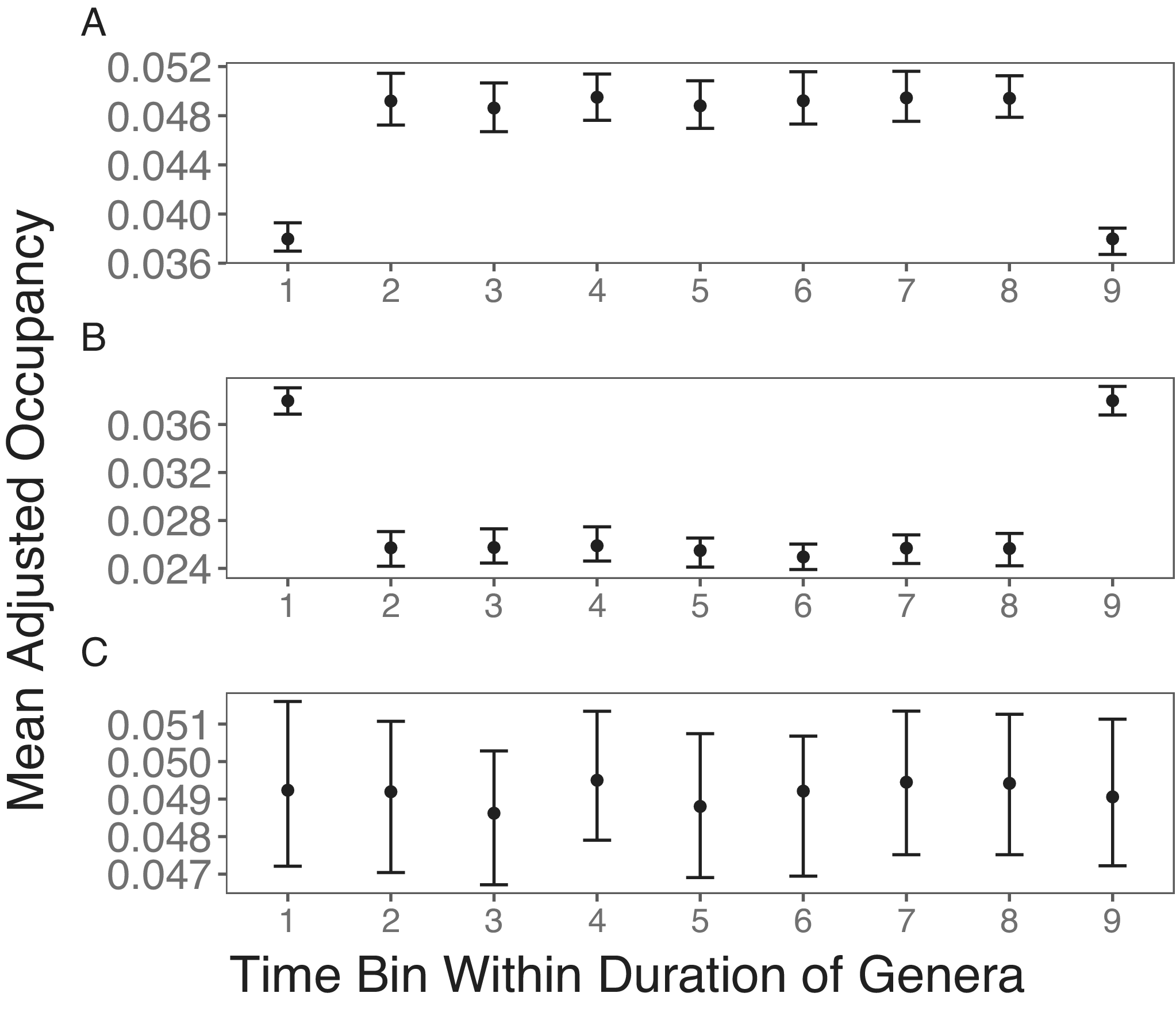
The simulation outcome shows that the punctuated rise and fall pattern, as found by Foote (Reference Foote2014), can be artificially generated by the fossil record, even when taxa do not show any changes in their occupancy probabilities through time. If unsampled taxa are simply excluded from occupancy estimates in intermediate time bins, the first bias from better sampling in boundary bins results in lower occupancies in the boundary bins (Fig. 1A). When such a pattern is averaged across taxa with different stratigraphic ranges, one would expect the short-lived peak in occupancy or range size found in previous studies (Jernvall and Fortelius Reference Jernvall and Fortelius2004; Foote Reference Foote2007). When missing taxa are replaced by zero, this only reverses the direction of bias (Fig. 1B). Finally, if I employ the proposed correction of conditioning the boundary time bins to follow that of intermediate time bins, the expected stable occupancy trajectory is found (Fig. 1C).
Simulation results of stable occupancy trajectories. A, Taxa with zero occupancies are excluded from the mean occupancy within each time bin, resulting in the bias of lower occupancy in boundary bins. B, Taxa that are not sampled are given an occupancy of zero, resulting in the bias of higher mean occupancies in boundary bins. C, Taxa with zero occupancies are excluded from the mean occupancies. Taxa in the first and last time bins are also excluded from the mean occupancies if they are not sampled in the second and penultimate bins, respectively. This treatment results in the expected stable mean occupancy trajectory.

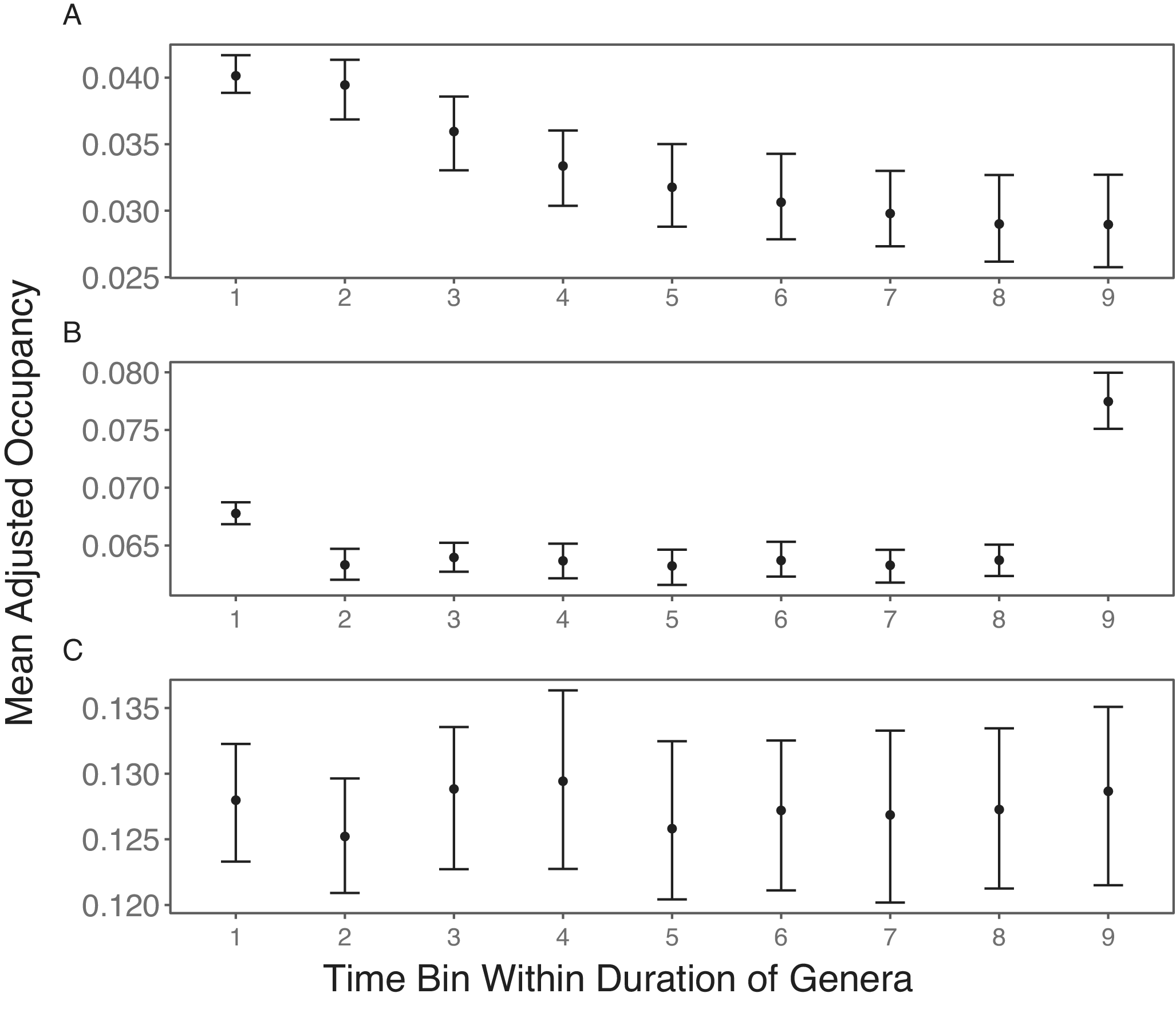
To test the effects of varying the number of sampled sites, I also performed the same simulations with the number of sites decreasing through time. Without subsampling, there is a decreasing trend in mean observed occupancy (Fig. 2A). This agrees with how the strength of positive bias is stronger with fewer sites (Chao et al. Reference Chao, Hsieh, Chazdon, Colwell and Gotelli2015; Foote Reference Foote2016).
Simulation results of stable mean occupancy trajectories with sequentially increasing number of sites. In all three scenarios, taxa are included in the mean occupancies of the first and last bins only if they are present in the second and penultimate bin, after subsampling (if performed), respectively. A, No subsampling is performed, resulting in sequentially decreasing occupancy. B, Each time bin is subsampled to 30 sites, and a taxon is only included in a time bin’s mean occupancy if it has nonzero occupancy in that bin after subsampling. This does not eliminate the bias from differences in the number of sampled sites. C, Each time bin is subsampled to 30 sites. A taxon is only included in the mean occupancy of a time bin if it has nonzero occupancy in that bin, as well as in both boundary bins, after subsampling. This results in the expected stable occupancy.

Next, I applied subsampling to the simulation outputs. With this, I still do not observe the expected stable range trajectory (Fig. 2B), with the boundary bins having higher occupancy than the intermediate bins. The last bin, especially, has extremely high occupancy.
The pattern in Figure 2B arises because the sampling of a taxon in a time bin after subsampling depends on it also being sampled in boundary bins before subsampling. Naturally, taxa in a bin are included in the mean occupancy of that bin only when they still have nonzero occupancies after subsampling. Again, taxa must also be sampled in the boundary bins. However, it is sufficient that they are sampled in the boundary bins before subsampling. Thus, even after subsampling, there remains a dependency of mean taxon occupancy on the sample size before subsampling. Intermediate bins have lower mean taxon occupancies in Figure 2B, because aside from the focal bins themselves, they are dependent on the large sample sizes of both boundary bins before subsampling. Because I applied the correction to the first bias of better sampling in boundary bins after subsampling, the mean taxon occupancy in the first bin is dependent on the first bin itself after subsampling, the last bin before subsampling, and a designated intermediate bin after subsampling. Given that boundary bins depend on two subsampled time bins and one time bin before subsampling, they have higher mean taxon occupancies than intermediate bins. The last bin has the highest mean taxon occupancy, because it depends on the first time bin pre-subsampling, which has the lowest sample size due to the sequentially increasing samples.
To ensure all sampling probabilities depend on the same sample sizes, all taxa that do not occur in both boundary bins post-subsampling are excluded. With this, the mean taxon occupancy in each time bin is equally dependent on being subsampled in that time bin itself and two other post-subsampled bins. Hence, the expected stable trajectory is now found (Fig. 2C). This suggests that subsampling is an optimal approach for looking at relative occupancy trajectories, but only when one has a large amount of data to work with.
Empirical Pattern
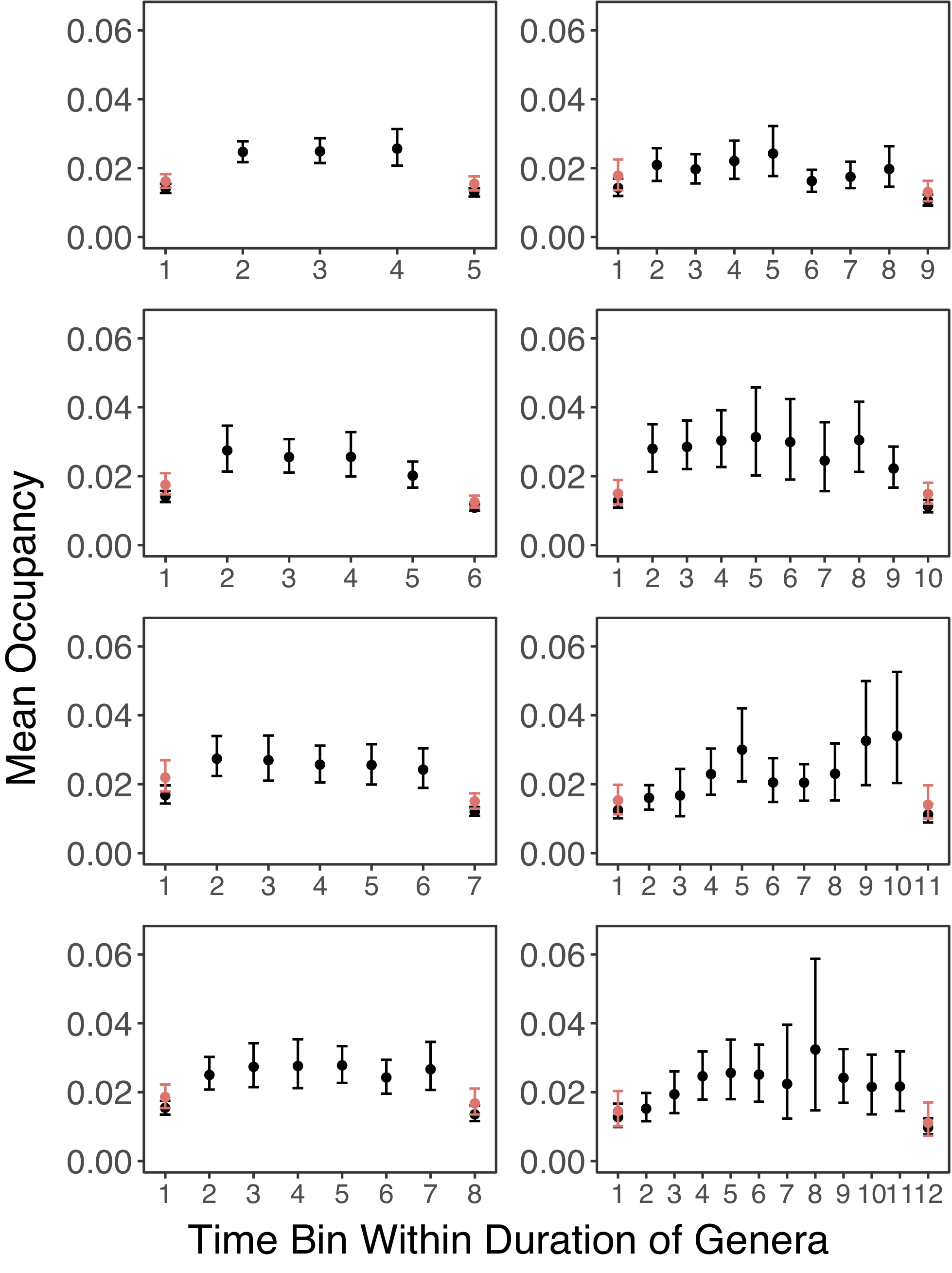
Looking at the empirical pattern without the correction for better sampling in boundary bins, Figure 3 shows a general trend of quick rise in occupancy, followed by stable occupancy for a few time bins, then a sudden decline in the last time bin. This trend is consistent across genera with different apparent stratigraphic ranges. The pattern is also similar when mass extinctions are not excluded (Supplementary Fig. S1).
Mean occupancy trajectories of genera from stratigraphic ranges of 5 to 12 time bins. Genera that went extinct during mass extinctions or survive close to the Recent are excluded. If a genus is not sampled in a time bin, it is excluded from the mean occupancy for that time bin. Error bars represent 95% confidence intervals from bootstrap resampling. For the results shown in red, genera are only included in the mean occupancies of the first and last time bins if they are sampled in the second and penultimate time bins, respectively.

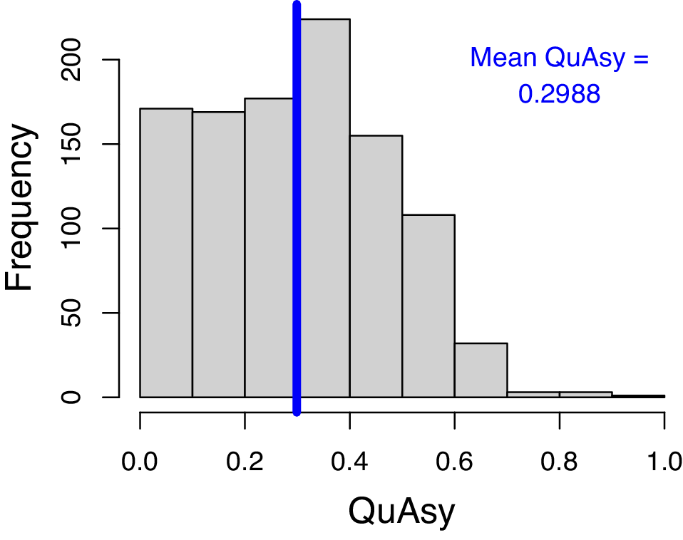
The mean QuAsy for individual trajectories of genera without gaps in their stratigraphic ranges is 0.2988. The histogram (Fig. 4) also shows that most of the trajectories should be mainly symmetric, but still with parts that are asymmetric. While this result still supports past studies finding symmetric trajectories (Foote Reference Foote2007; Liow and Stenseth Reference Liow and Stenseth2007), there is a considerable degree of asymmetry that should be explained.
Histogram of Quantified Asymmetry (QuAsy) values calculated from the occupancy trajectories of individual genera that do not have gaps within their stratigraphic ranges. The vertical blue line shows the mean QuAsy value. QuAsy values are scaled to be from 0 to 1, with 0 representing complete symmetry.

After the correction is applied to fix the first bias of better sampling in boundary bins, the mean occupancy in these bins increases for the occupancy trajectories of all apparent stratigraphic ranges (Fig. 3). For some stratigraphic ranges, this changed the punctuated pattern to be more of a gradual rise or a gradual fall. However, for other groups, a punctuated pattern remains. Nevertheless, this suggested that the bias in the boundary stages has made the punctuated pattern seem more prominent than it is. After the correction is applied to the second bias of incomplete durations in boundary bins, there is a gradual rise in occupancy from the first to the third stage, but more stable occupancy in the third-last and penultimate stage until an abrupt fall in the last stage (Fig. 5). This suggests that some of the abrupt rise that existed before this correction (Fig. 3) is due to incomplete duration in the first stage. This also fits with Foote’s (Reference Foote2005) result that pulsed extinction is more prevalent than pulsed origination. Furthermore, it would explain why incomplete duration bias has a stronger effect on origination than extinction, as taxa should be more likely to be extant throughout their boundary bins if their appearances or disappearances are pulsed.
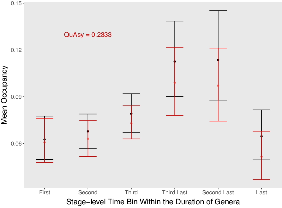
Mean occupancy in the second to the last substages of genera that were sampled in the first substages of their first three stage-level time bins, and in the first to the penultimate substages of genera that were sampled in the last substages of their last three stage-level time bins. Genera that went extinct during mass extinctions or that survive close to the Recent are excluded. For the first and last stage-level time bins, only genera that were also sampled in their second and penultimate stage-level time bins, respectively, are included. The fall in occupancy seems gradual, but there is an abrupt drop at the final bin. Mean occupancies adjusted by Chao et al.’s (Reference Chao, Hsieh, Chazdon, Colwell and Gotelli2015) method are shown in red. The Quantified Asymmetry (QuAsy) value, scaled from 0 to 1, calculated from this mean trajectory is also given.

One potential problem with the correction approach used is that the very first and last substages are excluded when calculating occupancies. If lower occupancies were not found in boundary stages, it is possible that those lower occupancies were thrown away with the first and last substages. However, I still observed lower occupancies in the first and last stages, so in this regard, this limitation does not cause ambiguities. The other pattern of interest is whether the abrupt rise and fall is real. An abrupt fall is observed, but not an abrupt rise (Fig. 5). Again, the lack of an abrupt rise may be due to the abrupt rise happening in the very first substage that was thrown away. However, it can at least be inferred that a punctuated fall is real. Most genera that are assignable to substages are from the Ordovician and Silurian, so it is uncertain whether this pattern is representative of the Phanerozoic as a whole.
After adjusting for the number of sampled sites using Chao et al.’s (2015)approach, the general trend remains similar (Fig. 5). This suggests that the bias from a varying number of sampled sites did not influence the pattern. However, as discussed earlier, it would be ideal to perform subsampling on a more complete dataset.
The QuAsy of the mean trajectory after correcting for the second bias is 0.2317 (Fig. 5). This is lower than the QuAsy value of 0.2988 without the correction. However, these two values may not be comparable for two reasons. First, the QuAsy with the correction is measured from the mean trajectory while the QuAsy values without the correction are measured from individual trajectories. Averaging may cause them to be more symmetric (Hohmann and Jarochowska Reference Hohmann and Jarochowska2019). Second, as discussed earlier, the trajectory after correcting for the second bias contains only the first three and last three time bins. More data with “substage-level” occurrences will be needed to obtain complete individual trajectories while correcting for the second bias.
Discussion and Conclusions
In this study, I measured occupancy trajectories and demonstrated three possible biases that have not been accounted for in previous studies of occupancy and range size trajectories. While there are many established methods in occupancy modeling, such as those that account for unobserved presences (Liow Reference Liow2013; MacKenzie et al. Reference MacKenzie, Nichols, Royle, Pollock, Bailey and Hines2017; Reitan et al. Reference Reitan, Ergon and Liow2023), I opt to use Foote’s (Reference Foote2014) approach of counting geographic cells and calculating the average occupancy trajectory. Given that the three biases here have not been studied in detail before, the relatively simple approach of counting geographic cells allows the effects of these biases on occupancy trajectories to be much more clearly shown. For future work, it may be possible to account for these biases when applying more complex occupancy modeling methods.
For the first bias of better sampling in boundary bins, the solution of excluding boundary bin taxa from the mean occupancy trajectory if they do not occur in intermediate bins is easily applicable, and most of the data are retained. The bias and solution should apply to most studies that involve computing mean occupancy when taxa have unsampled time bins within their stratigraphic ranges. However, the bias does not apply when one is not looking at the mean occupancy but the occupancy trajectories of individual taxa, such as in the studies by Foote et al. (Reference Foote2007) or Liow et al. (Reference Liow, Skaug, Ergon and Schweder2010). Nevertheless, it can be difficult to infer occupancy trajectories from individual occupancy trajectories when gaps are abundant in the record. If sampling is relatively complete, such as for microfossils (Liow and Stenseth Reference Liow and Stenseth2007; Liow et al. Reference Liow, Skaug, Ergon and Schweder2010), the bias should largely be mitigated, as it is dependent on there being unsampled time bins.
Correcting the first bias dampened the punctuated effects in rises and falls, especially revealing that genera do not expand their geographic ranges after their origination as suddenly as it seemed without correcting for the bias (Fig. 3). However, the difference is not as drastic as the simulation may lead us to believe (Fig. 1). This may simply be a stochastic effect from not having a large number of empirical samples. Another possible reason is that the bias is strong when differences in occupancy among taxa are consistent throughout the trajectory, as the selection for widespread taxa will be consistently influenced by both the boundary and intermediate bins. This assumption holds true in the simulation, with each taxon having a constant occupancy trajectory. However, in the empirical data, a taxon that is relatively more widespread in one interval may become less widespread than other taxa in the next.
The solution proposed for the second bias is to use substage-level occurrences as constraints to measure occupancies of boundary and intermediate bins in comparable proportions. However, this solution can provide ambiguous results. As discussed earlier, the solution throws away the very first and last substage-level time bins, which may represent important periods of geographic range expansion and contraction within the duration of a taxon. Although the solution is sufficient to support the presence of a sudden geographic range contraction preceding extinction, further development of methods will be needed to test whether the pattern of range expansion post-origination is real. Using groups that can be subdivided into time bins finer than the ones in this study, such as graptolites, may also be helpful for mitigating this bias (Foote et al. Reference Foote, Sadler, Cooper and Crampton2019; Crampton et al. Reference Crampton, Cooper, Foote and Sadler2020). Unlike the first bias, this second bias applies to both the mean occupancy and individual occupancy trajectories of taxa. Thus, there may be value applying this even to studies that use individual trajectories (Foote et al. Reference Foote2007).
For the third bias of varying number of sampled sites, applying Chao et al.’s (Reference Chao, Hsieh, Chazdon, Colwell and Gotelli2015) method did not produce any notable changes to the occupancy trajectory (Fig. 5). However, that approach does not account for the dependency of occupancy in one time bin on sampling in other bins within a temporal occupancy trajectory. One solution to this is subsampling, but that involves throwing away taxa that are not subsampled in both boundary bins, which would eliminate most of the taxa in a dataset. Thus, this approach may only be appropriate for data with taxa that are well sampled geographically throughout their stratigraphic ranges, such that we can subsample a large number of sites to increase the chances of taxa being subsampled in their boundary bins. When using a dataset such as the one in this study, a better option may be to further extend approaches such as Chao et al.’s (Reference Chao, Hsieh, Chazdon, Colwell and Gotelli2015) or Foote’s (Reference Foote2016) to account for dependencies between time bins.
The fact that genera with zero occupancies were excluded from the study may mute any large drops in occupancy, working against finding a random walk or any types of fluctuating pattern. As discussed earlier, treating those genera with zero occupancies biases the boundary bins relative to the intermediate bins. However, looking at the mean occupancy trajectory of only intermediate bins with zero occupancies included, the pattern remains similar to when they were excluded (Supplementary Figs. S4, S5). Thus, it is unlikely that any fluctuations in occupancies were masked by this effect. It is also possible that using the mean occupancy trajectory may eliminate any fluctuations that exist in the occupancy trajectories of individual taxa. The new occupancy trajectory uncovered in this study gives further insight into the processes driving the pattern (Fig. 5). For instance, the pattern is inconsistent with geographic range size changes produced by an unbiased random walk (Foote Reference Foote2007; Pigot et al. Reference Pigot, Owens and Orme2012). While the pattern does not support a complete random walk, it is uncertain whether the geographic range size changes seen here depend on the range values already occupied. Further testing will be needed in a manner similar to that done by Žliobaitė (Reference Žliobaitė2024), wherein species’ maximum range expansion curves were found to be linear, similar to Van Valen’s (Reference Van Valen1973) species’ survivorship curves.
Aside from simply testing whether the pattern can be described by a random walk, it is also crucial to understand the biotic and abiotic drivers behind occupancy trajectories. As seen in Figure 5, rather than gradually approaching extinction, genera’s occupancies suddenly decrease in their final time bins of appearance. This suggests that sudden physical perturbations may be responsible for a majority of genera’s extinctions. However, it is still unclear whether these occupancy drops are from the same types of events as the pulsed extinctions observed from the fossil record (Foote Reference Foote2005). It will be beneficial to test whether genera that show sudden occupancy drops tend to do so at the same time, relative to genera that show gradual occupancy decreases.
Aside from abiotic factors, a sudden decrease in extinction before extinction may also reflect invasions of competitors, given that interspecific competition has been shown to disrupt geographic ranges (Price and Kirkpatrick Reference Price and Kirkpatrick2009). This pattern also fits with the Red Queen hypothesis (Van Valen Reference Van Valen1973), given that there is no progressive decline in occupancy with age. However, it is still debatable whether the risk of extinction may increase with age in ways that are not reflected in occupancy values. For example, there may be progressive specialization with age that causes taxa to be more prone to speciation (Whitlock Reference Whitlock1996). If niche breadth is not always associated with occupancy or range size (Cardillo et al. 2016), this progressive specialization may not be reflected in occupancy trajectories.
The occupancy trajectories also start off with relatively small occupancy, corroborating the hypothesis that populations often start small (Vrba and DeGusta Reference Vrba and DeGusta2004). However, it is uncertain how much conclusive evidence can be drawn regarding population dynamics, given the data used are at the genus level. The timing of range size or population expansion is also ambiguous, given occupancy was not measured in the first substage due to the solution for the second bias. One possible interpretation, given the occupancy trajectories found here, is that it may take much longer than the ~1 million year period hypothesized by Vrba and DeGusta (Reference Vrba and DeGusta2004) before populations start expanding. An alternative interpretation is that the short period of range expansion was thrown away with the first substage.
Genera also tend to increase gradually in occupancy through time after origination, with the third-last and second-last time bins having significantly higher occupancies than the first three time bins (Fig. 5). This is also reflected in there being some degree of asymmetry in the trajectories (Figs. 3, 5). One possible explanation for the gradual occupancy rise is that species continually overcome their geographic range limits through adaptation (Kirkpatrick and Barton Reference Kirkpatrick and Barton1997). Testing this may require data on the trajectories of taxa’s niche breadths in addition to their occupancy trajectories. On the other hand, there may be gradual rises in occupancy without adaptation if taxa shift their geographic distributions to track environmental changes (Davies et al. Reference Davies, Purvis and Gittleman2009). While taxa could either be subject to occupancy increases or decreases from environmental forcings, if taxa that expand their ranges are more likely to survive, then mean range sizes should gradually expand on average.
Aside from geographic range size or occupancy, the successes of genera have been measured by species richness (Foote Reference Foote2007). In addition, how geographic ranges are distributed among species, as well as the number of species per genus, may impact range sizes at the genus level (Foote et al. Reference Foote2016; Tomašových and Jablonski Reference Tomašových and Jablonski2017). Thus, I also look at the trajectory of mean species richness through time (Supplementary Fig. S6). There are significant differences from the mean occupancy trajectory, such as long-term declines in species richness through time. This suggests that genera’s geographic range sizes are not controlled by species richness alone, although the effects of the constituent species’ range sizes, as well as how they are distributed in space, remain to be seen.
In conclusion, corrections were proposed and tested for the first two biases of better sampling and incomplete durations in boundary bins. The third bias of varying number of sampled sites, as well as its solution through subsampling, is tested through simulations, but there are not sufficient empirical data to apply it here. After these changes, the current average occupancy trajectory for marine animal genera does not have a sudden rise after the first stage, but seems to rise slowly throughout a genus’s duration, with a sudden fall preceding extinction. However, future work to solve ambiguities remains, such as whether a sudden occupancy may have been thrown out with the first substage, and whether the occupancy trajectory in intermediate bins is more dynamic than it appears. Much further testing will also be required to infer the biotic and abiotic drivers behind these occupancy patterns.
Acknowledgments
I am grateful to M. Foote and S. Finnegan for valuable discussions on the project. M. Foote also provided the vetted PBDB data used here. P. Wagner, N. Hohmann, and two anonymous reviewers provided helpful feedback.
Competing Interests
The author declares no conflicts of interest.
Data Availability Statement
Data, code, and Supplementary Material available from the Zenodo Digital Repository: https://doi.org/10.5281/zenodo.17612909.

 Open access