


1. Introduction
Multi-rotor unmanned aerial vehicles (UAVs) have become increasingly popular for various commercial applications such as inspection, search and rescue, and remote sensing. In recent years, there is now a strong push in both the research and commercial fields to increase the autonomy of UAVs so they can improve the efficiency of traditionally slow or costly tasks.
One essential task for truly autonomous operation is exploration planning. A fully autonomous system should be able to explore and map its operating environment without detailed prior information. Many existing works work around this by employing sampling- or frontier-based exploration methods. These methods generate successive poses to visit based on defined heuristics estimating the amount of information gained by visiting each candidate pose. These heuristics are often weighted to minimize exploration time [Reference Zhou, Zhang, Chen and Shen1, Reference Cieslewski, Kaufmann and Scaramuzza2] or maximize information gain [Reference Schmid, Pantic, Khanna, Ott, Siegwart and Nieto3, Reference Song and Jo4]. These generalized methods perform well when no prior structural information regarding the operating environment is available. However, because of this gearing towards completely unknown environments, existing approaches are not designed to exploit any partial prior information regarding the structure of the area. The lack of exploitation of available information limits the performance of existing methods in semi-structured environments such as plantation forests, apple orchards, or vineyards. These areas generally follow a semi-structured layout, where high-level structural information is defined but not necessarily implemented, leading to some variation in spacing between neighboring trees.
Of particular interest for this work is under-canopy surveying of plantation forests, which poses a different set of requirements than previous exploration path planning works. The plantation forest environment itself is laid out in a semi-structured manner, where trees are planted in successive parallel rows. However, the tree-to-tree and row-to-row spacings vary due to the land geography or plantation process. Unlike the unknown environments that previous works assume, the direction and approximate spacing of rows of trees in a plantation forest are known ahead of time. But, this information cannot be incorporated into existing exploration methods, as no detailed structural information is known. Furthermore, under-canopy forestry surveys do not need to fully map the ground or any points high up in the canopy since these can be easily acquired via data airborne laser scanning (ALS). For plantation forest surveys, the UAV does not need to observe the entire volume; it is sufficient only to observe every tree in the area. Therefore, existing methods favoring reconstruction accuracy will generally produce suboptimal survey paths from unnecessary volumes being explored.
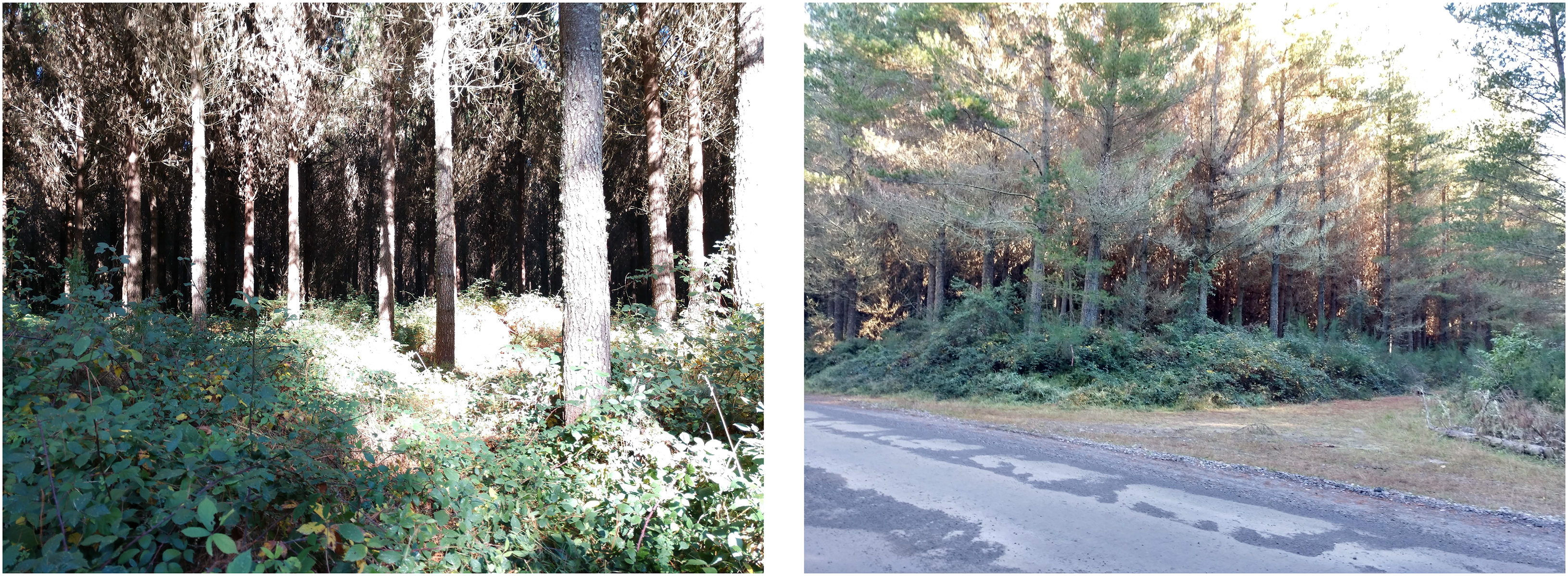
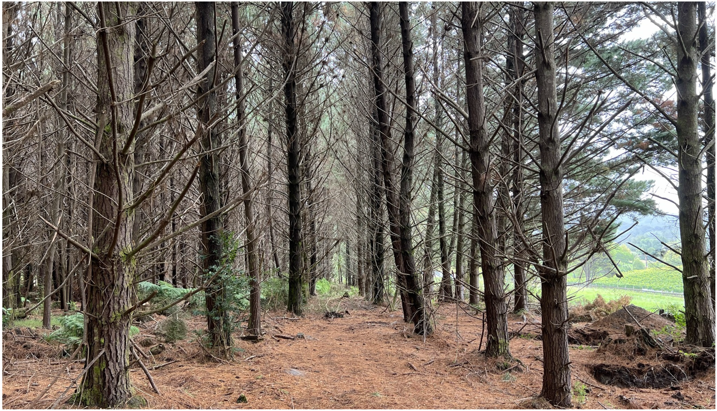
Plantation forests in New Zealand are a hostile environment for any ground-based robots. This hostility stems from the presence of large amounts of undergrown covering the majority of the ground space, particularly towards the later stages of growth. Fortunately, plantations are often pruned up to a height of 5−6 m, producing a traversable corridor in the space between the top of the undergrowth and the bottom of the lowest branches. This effect can be seen in typical New Zealand plantations shown in Fig. 1.
Typical New Zealand plantation forests. Note the presence of a traversable flight corridor between the undergrowth and low branches.
This paper seeks to explore potential performance gains from following a semi-structured exploration pattern when traversing typical New Zealand plantation forest environments. First, probability distributions modeling the spatial layout of typical plantation forests are extracted from point clouds of real plantation forests. These distributions are used to procedurally generate a number of realistic testing environments. Three variations of a waypoint placement method based on a lawnmowing pattern are proposed to maximize coverage efficiency. Next, the performance of these methods is evaluated in simulation against state-of-the-art exploration planners. Finally, a flight test is performed in a local stand of trees to demonstrate the proposed method’s ability to operate in outdoor environments.
The contributions of this paper are as follows:
-
• A set of probability distributions modeling the spatial layout of a typical New Zealand plantation forest.
-
• An exploration method for plantation forest environments that forego traditional heuristic-based goal selection in favor of generalized structural information.
-
• Evaluation of the performance of the aforementioned structured exploration approach compared to state-of-the-art exploration planners.
Towards these contributions, Section 2 reviews notable works in this area. Section 3 outlines the parameters and probability distributions used to describe typical New Zealand plantation forests. Section 5 evaluates high-level 2D performance in the presence of generated obstacles, and Section 6 outlines performance testing in 3D against other prevailing fast exploration methods. Finally, flight testing is conducted in a real plantation forest in Section 7.
2. Related works
2.1. Robot exploration
Autonomous exploration planning with multirotor UAVs has attracted interest in recent years, likely due to the increased availability of low-cost, high-performance sensors, and computers. The objective of this task is to produce a completed map of the region of interest in the minimum amount of time. In contrast to pure path planning approaches presented in literature such as refs. [Reference Zhou, Pan, Gao and Shen5–Reference Dönmez, Kocamaz and Dirik9] which aim to find the most optimal path to a specific goal, exploration planning aims to find the most optimal path which observes the entirety of some environment. Because exploration planning encompasses path planning, many approaches employ waypoint selection, with the actual traversal path being generated by existing methods.
Depending on the use case, completion of the map can range from localization of an object to observing the entire traversable volume in the environment. The exploration objective also differs depending on the application; some examples are minimizing exploration time [Reference Zhou, Zhang, Chen and Shen1, Reference Cieslewski, Kaufmann and Scaramuzza2, Reference Duberg and Jensfelt10, Reference Dharmadhikari, Dang, Solanka, Loje, Nguyen, Khedekar and Alexis11], maximizing reconstruction accuracy [Reference Schmid, Pantic, Khanna, Ott, Siegwart and Nieto3, Reference Song and Jo4], dealing with multirobot and battery limitations [Reference Cesare, Skeele, Yoo, Zhang and Hollinger12], object search [Reference Dang, Papachristos and Alexis13], or multiagent exploration [Reference Guastella, Cantelli, Longo, Melita and Muscato14, Reference Collins, Ghassemi, Esfahani, Doermann, Dantu and Chowdhury15]. These methods can be broadly classified into sampling- or frontier-based methods.
Frontier-based exploration was first proposed in ref. [Reference Yamauchi16], which defined frontier regions as the boundary between explored and unexplored space. The region of interest can be fully surveyed by continuously generating and visiting every observed frontier, with the process concluding when all frontiers are observed. Advancements in frontier-based exploration methods generally focus on frontier selection. In ref. [Reference Yamauchi16], the planner always selects the closest frontier from the current location as the next location to visit. Ref. [Reference Cieslewski, Kaufmann and Scaramuzza2] instead picks the frontier within the current sensor field of view, which minimizes velocity change of the UAV, allowing for sustained high-velocity flight throughout the exploration process, and is shown to outperform the method presented in ref. [Reference Yamauchi16]. In ref. [Reference Meng, Qin, Chen, Chen, Sun, Lin and Ang17], a two-tiered approach is used, where frontiers are first extracted, and a traveling salesman problem is formulated to determine the order in which the frontiers should be visited. Ref. [Reference Zhou, Zhang, Chen and Shen1] follows a similar approach, except frontiers are sampled and stored in an incrementally updated frontier information structure for computational efficiency reasons; a local segment of the tour is then used to generate a dynamically feasible trajectory for the UAV to follow. In ref. [Reference Dai, Papatheodorou, Funk, Tzoumanikas and Leutenegger18], the octomap map representation is exploited to reduce computation costs due to implicit clustering of frontiers by early termination of voxel lookups.
Sample-based methods, on the other hand, use the concept of next best view (NBV) [Reference Connolly19], originally designed to determine the best viewpoints for 3D scene reconstruction. NBV defines the concept of information gain—i.e., how much information can be extracted from the environment at a specific viewpoint. A sample-based method randomly samples poses within the already explored volume of the environment and estimates the information gained by visiting that pose. Similar to frontier-based exploration, the performance of these methods is also heavily dependent on the choice of the sampling method. In ref. [Reference Dharmadhikari, Dang, Solanka, Loje, Nguyen, Khedekar and Alexis11], sampling is provided by using a library of motion primitives defining available trajectories. Ref. [Reference Papachristos, Khattak and Alexis20] uses rapidly exploring random trees (RRT) [Reference LaValle21] to sample the explored space. Ref. [Reference Bircher, Kamel, Alexis, Oleynikova and Siegwart22] takes the concept further with receding horizon NBV (RH-NBV); similar to the RRT-based approach, the explored region is sampled to determine the NBV for exploration, and a path is generated to traverse to this new location. Only the first node to this path is executed before the region of interest is resampled for more optimal poses. Historically visited poses are used in ref. [Reference Witting, Fehr, Bähnemann, Oleynikova and Siegwart23] to guide the exploration and avoid local minima. Autonomous exploration planner, a hybrid approach combining RH-NBV and frontier-based exploration, is proposed in ref. [Reference Selin, Tiger, Duberg, Heintz and Jensfelt24] to encourage robot movement towards unexplored regions. A rewiring approach similar to the one taken in RRT is used in ref. [Reference Schmid, Pantic, Khanna, Ott, Siegwart and Nieto3] to maintain and refine a single tree for the entire exploration process. More recently, a probabilistic roadmap (PRM) [Reference Kavraki, Svestka, Latombe and Overmars25] representation is proposed in ref. [Reference Xu, Deng and Shimada26], which incrementally constructs a PRM for faster planning compared to RRT-based methods.
2.2. Forest surveying
Surveying of plantation forests is often done as a high-level management task, predominantly related to estimating the available volume and quality of merchandisable wood with the intent of estimating the monetary value of a specific stand of trees. The process for assessment of a plantation in New Zealand uses MARVL [Reference Deadman and Goulding27], a regression-based method relying on extrapolating structural information retrieved from a small set of trees. To collect data for MARVL, several systematic small plots are surveyed through a process known as cruising [28], where a variety of parameters such as tree height, diameter at breast height, log defects (e.g. knots, pruned height, etc.), and tree height is noted for every tree in the small plot. Because of labor limitations, the plots are generally circular in size with a diameter between 20 and 30 m, and a small total area of the forest is surveyed. More recently, there has been a push for the use of ALS or terrestrial laser scanning (TLS) to acquire high-density point clouds, which can be post-processed to extract required information [Reference Hyyppä, Hyyppä, Hakala, Kukko, Wulder, White, Pyörälä, Yu, Wang, Virtanen, Pohjavirta, Liang, Holopainen and Kaartinen29–Reference Hyyppä, Hyyppä, Hakala, Kukko, Wulder, White, Pyörälä, Yu, Wang, Virtanen, Pohjavirta, Liang, Holopainen and Kaartinen32]. TLS benefits significantly from the ultra-wide field-of-view (FOV) of rotating LiDARs, as rays projected in, effectively, any direction will return useful data about the region. Omnidirectional rotating sensors such as the Velodyne Puck and Ouster OS series are popular due to cost, weight, and power limitations.
Previous attempts at autonomous navigation within plantation forest-like environments are generally focused on autonomously navigating down a single row. Works in this area include, for example, refs. [Reference Jiang33, Reference Chiella, Machado, Teixeira and Pereira34] both use an artificial potential field (APF)-based approach for collision-free navigation within plantation forests, while our previous work [Reference Lin and Stol35] extends this to explore multiple rows. The work in ref. [Reference Cui, Lai, Dong and Chen36] uses a manually planned trajectory and focuses on the localization and reproduction aspects of the problem. A planar LiDAR is used in ref. [Reference Higuti, Velasquez, Magalhaes, Becker and Chowdhary37] to identify rows with a foilage-covered corn field, and navigation is completed with a ground-based robot. The common theme among all of the mentioned approaches is that none have quantified the performance of their method against other exploration planning methods in the literature.
3. Plantation forests
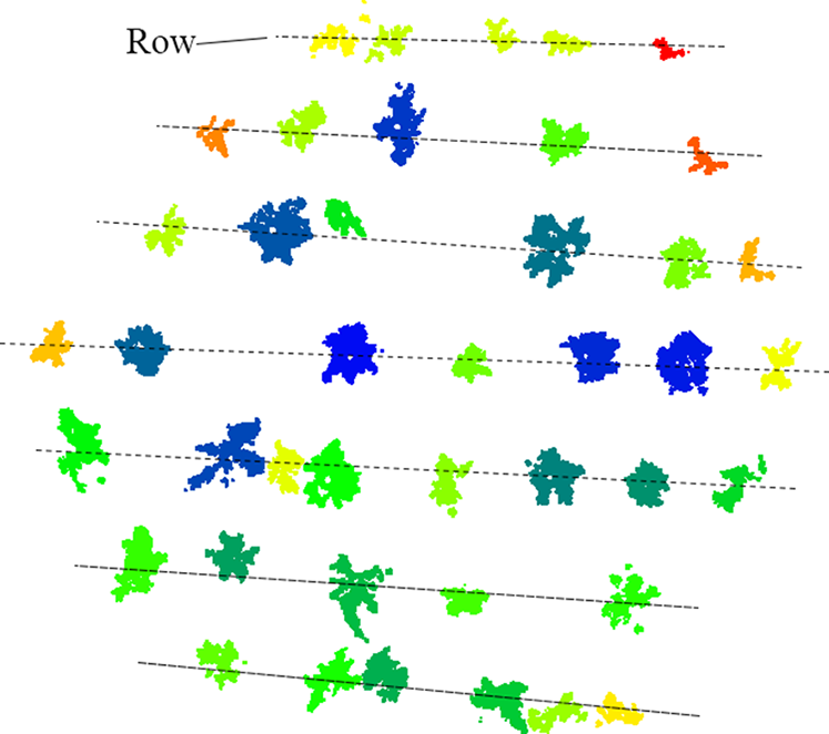
Typical plantation forests within New Zealand consist of Pinus Radiata planted ideally on a regularly spaced square grid to allocate an approximately consistent land area to each tree. The spacing of trees on this grid depends on the plantation’s density, typically starting at 800−1200 stems/ha at plot establishment and dropping to 200−350 stems/ha at harvest. The corresponding drop in density is due to a process known as thinning, where stems with defects or a low rate of growth are cut down to make space for higher-quality stems to grow [Reference Maclaren38]. In reality, planting on a perfect grid is difficult; therefore, plantations are typically established on a row-by-row basis, with individual parallel rows of trees planted sequentially. The effect of this can be seen via a horizontal cross-section of a New Zealand plantation forest, shown in Fig. 2. Distinct parallel rows are apparent within the environment with consistent row spacing but no consistent structure in the orthogonal direction.
Horizontal cross-section of a typical plantation forest. Separate trees are shown as clusters of the same color. Row structure highlighted with dotted lines.
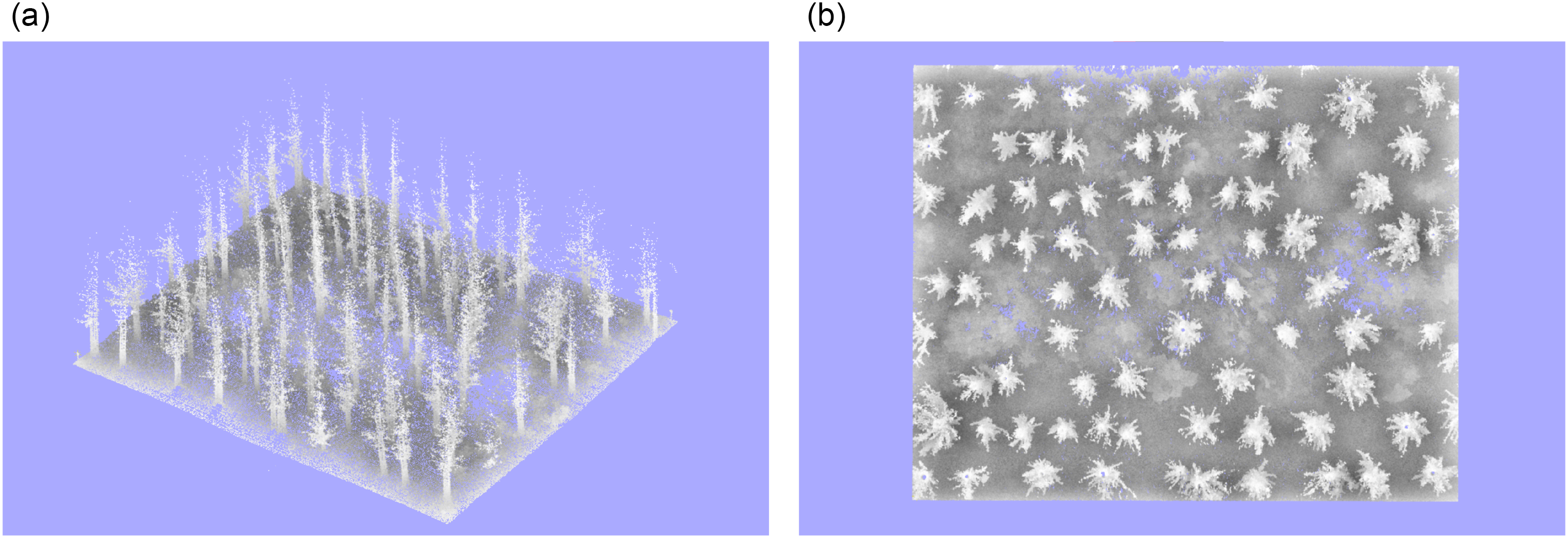
(a) Isometric and (b) top-down view of the first point cloud used for parameter extraction. The point cloud in (b) is aligned such that the rows are aligned in the horizontal direction.
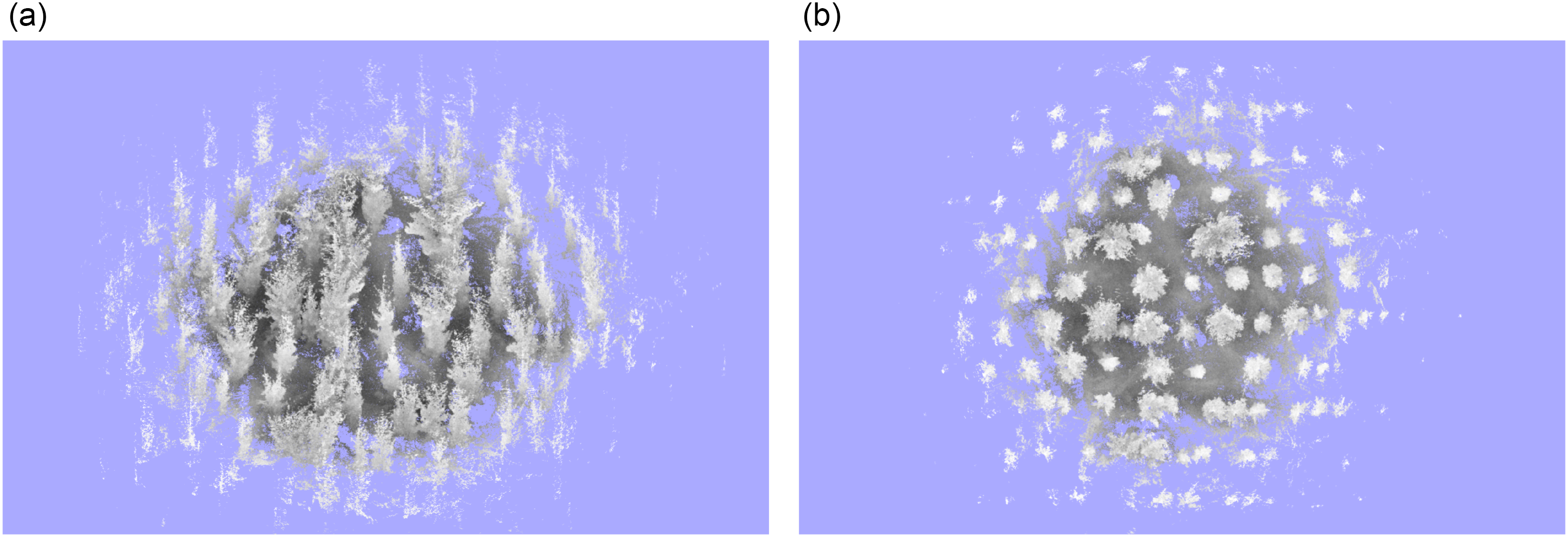
(a) Isometric and (b) top-down view of the second point cloud used for parameter extraction. The point cloud in (b) is aligned such that the rows are aligned in the horizontal direction.
3.1. Examined environments
Two point cloud scans of typical New Zealand plantation forests have been provided by Scion (Scion Research, 2019), each sampled using a Zeb Revo handheld LiDAR scanner. Due to accessibility constraints, both environments contain pruned trees on flat terrain with little undergrowth inhibiting movement through the area. The first environment shown in Fig. 3 is precropped to approximately 40 by 35 m and contains 74 trees arranged in nine rows; each stem is pruned to approximately 4 m above ground level. The second environment shown in Fig. 4 contains a high-density circular section with a diameter of approximately 30 m in the center, along with unused low-density partial trees outside of this area. This scan consisted of 48 usable trees arranged in seven rows pruned to approximately 5 m. Neither samples contain sufficient branching to completely occlude the vision of the sky.
3.2. Modelling the plantation environment
Because plantation forests are generally established on a row-by-row basis, we propose to treat the environment as a discrete set of nonevenly spaced parallel rows of trees during procedural generation. Therefore, it is sufficient to model the row spacing, tree spacing, and row deviation distributions as shown in Fig. 5(a) to generate tree positions in the environment procedurally.
(a) Isometric and (b) top-down view of the second point cloud used for parameter extraction. The point cloud in (b) is aligned such that the rows are aligned in the horizontal direction.
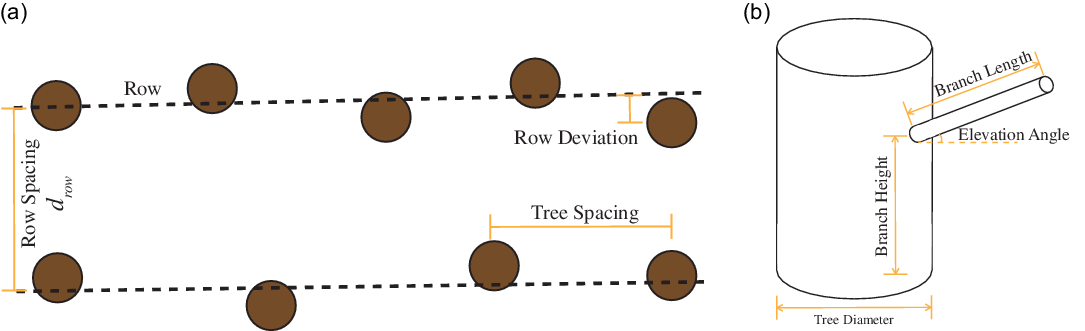
A tree can, in essence, be modeled as a large central cylinder, with many small cylinders as branches. Assuming that branches are randomly distributed around the tree, the branch can be approximated as a long cylinder with an elevation angle and length, as shown in Fig. 5(b). Each branch will have a corresponding height at which it joins the main stem.
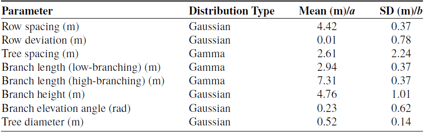
Extraction of the row and tree spacings is completed through ground plane removal, Euclidean clustering, decomposition into cylinder models, and finally, clustering of the cylinder models for parameters. The ground plane is removed by first applying Cloth Simulation Filter (CSF) [Reference Zhang, Qi, Wan, Wang, Xie, Wang and Yan39] to the entire point cloud. Next, Euclidean distance clustering via the PCL library [Reference Rusu and Cousins40] is used to segment the point cloud into individual trees. Finally, each segmented point cloud is decomposed into cylinder models using SimpleTree [Reference Hackenberg, Spiecker, Calders, Disney and Raumonen41]. Finally, this model is processed to determine each tree’s location and branching characteristics. Summaries of distribution types along with mean and standard deviation or a and b parameters for Gaussian and Gamma distributions, respectively, are shown in Table I, consisting of the averaged set of distributions from both environments.
3.3. Procedural generation
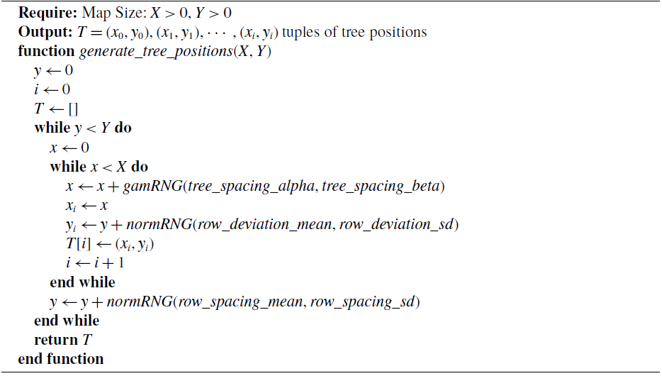
Once probability density functions of individual tree and tree placement parameters are available, a large number of simulated environments can be generated. For simplicity, it is assumed that no coupling effects exist between different trees, even when they are grown in close proximity. Branches are simply modeled as straight cylinders, and undergrowth is ignored. Under the assumption that all rows established in a plantation forest are approximately parallel, realistic tree positions can be synthesized row-by-row. The location of each row is generated as an offset from the previous row, and tree spacing and row deviation values are generated for each tree as an offset from the previous tree or current row. Algorithm 1 outlines the procedure used to generate the list of tree locations.
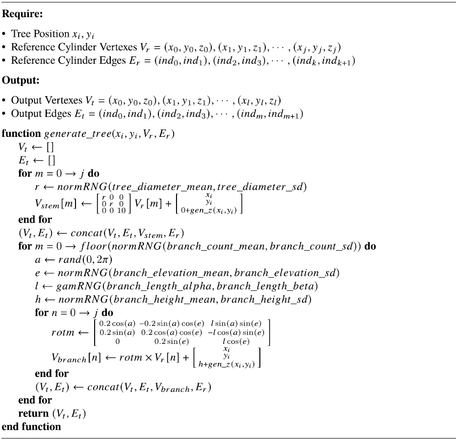
where normRNG and gamRNG generate random numbers in a normal and gamma distribution, respectively, using provided parameters. The mesh of a single tree can be generated as the concatenation of multiple cylinders. The main stem consists of a single large cylinder 10 m tall, and branches are produced through the transformation of cylinder coordinates. Consider a reference mesh consisting of a triangulated cylinder with a diameter and height of 1 m. Each tree can then be independently generated using Algorithm 2. Finally, a mesh of the entire environment can be generated by concatenating the ground plane with all of the generated trees.
Summary of parameters extracted from plantation forest point clouds.
Generate Tree Positions
4. Structured exploration
The goal of the proposed method is to minimize the time taken for a survey while maximizing the number and consistency of points sampled for each tree stem. One of the goals of the method is, therefore, to minimize the amount of overlap in the survey area. For this reduction to occur, the survey path should consist of long, straight sections to maintain consistent and high-speed operation. Our previous work [Reference Lin and Stol35] used a lawnmowing survey pattern with APF-based obstacle avoidance. Testing was limited only to regularly spaced environments without any untraversable regions. This work extends our previous method to work in realistic environments with unequal spacing and untraversable regions.
Generate Tree Geometry
4.1. Methodology
Because of the long, continuous flight corridors present within the scene, flying down one of these corridors is advantageous as direction changes are minimized. The entire region can be considered and visited if every row is traversed at least once, as the environment effectively consists of a finite number of rows.
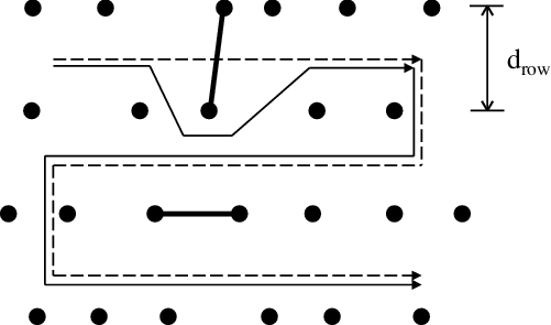
Diagram of paths with our proposed method. Initial path shown with dotted lines. Actual path is shown with solid lines. Solid circles represent stems in the environment, and thick black lines represent blockages.
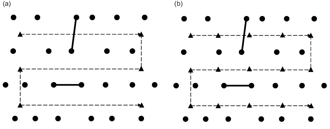
Initially planned waypoints for (a) Naive method and (b) Strict method. Waypoints are shown as triangles. The Greedy method uses the waypoints outlined in (b), and will generally follow the path laid out in (b).
The proposed method initially seeds exploration goals by sampling an ideal path through the environment, with the ideal path being aligned with the rows of trees. This process consists of a lawnmowing pattern with a spacing of $d_{\text{row}}$
between each traversed row. Since sensing the plantation environment is outsidethe scope of this work, the lawnmowing path is generated by assuming a fixed spacing represented as fixed coordinates in SE2/SE3 space in the low- and high-fidelity test cases, respectively. These waypoints are set as movement goals; therefore, the full 2D/3D volume can be used for traversal in the low- and high-fidelity test cases, respectively. Instead of generating viewpoints through NBV or frontier search, the UAV attempts to follow the ideal path for as long as possible by placing these waypoints along this path. Since environmental perception is not one of the goals of this paper,
$d_{\text{row}}$
between each traversed row. Since sensing the plantation environment is outsidethe scope of this work, the lawnmowing path is generated by assuming a fixed spacing represented as fixed coordinates in SE2/SE3 space in the low- and high-fidelity test cases, respectively. These waypoints are set as movement goals; therefore, the full 2D/3D volume can be used for traversal in the low- and high-fidelity test cases, respectively. Instead of generating viewpoints through NBV or frontier search, the UAV attempts to follow the ideal path for as long as possible by placing these waypoints along this path. Since environmental perception is not one of the goals of this paper, $d_{\text{row}}$
is assumed to be fixed to the average row spacing of 4.4 m. An A* path planner is then used to produce collision-free paths to traverse through all waypoints. An example of this with a single-blocked passage is illustrated in Fig. 6.
$d_{\text{row}}$
is assumed to be fixed to the average row spacing of 4.4 m. An A* path planner is then used to produce collision-free paths to traverse through all waypoints. An example of this with a single-blocked passage is illustrated in Fig. 6.
Three variants of this method are proposed, hereby referred to as the Naive, Strict, and Greedy methods. Each of these methods follows the same overall lawnmowing pattern, with the difference being the waypoint placement and selection process. The simplest one of the group is the Naive method, where waypoints are placed only at the vertexes of the pattern, as shown in Fig. 7(a). The Strict method introduces additional waypoints along each traversed row as shown in Fig. 7(b). Compared to the Naive method, the Strict method forces the UAV to traverse down the row as much as possible to improve coverage. A waypoint is skipped when there is no traversable path between the current location and the waypoint. On the other hand, the Greedy method does not enforce the order in which the waypoints need to be visited. The list of waypoints to visit is identical to those in the Naive approach. At each goal decision time, A* is used to search for paths to each unvisited waypoint, and the waypoint which can be reached with the shortest path is selected to be the next goal. This allows the UAV to deviate from the “ideal” waypoint visiting order should there be an easier-to-access waypoint. Like the Naive method, the Greedy method also places intermediate waypoints between the vertexes of the survey path. However, the waypoint spacing must be less than $d_{\text{row}}$
to encourage travel predominantly in the row direction. Experiments in this work use waypoints placed 4 m apart with
$d_{\text{row}}$
to encourage travel predominantly in the row direction. Experiments in this work use waypoints placed 4 m apart with $d_{\text{row}} = 4.5\;\text{m}$
. All three variants will produce identical flight paths when presented with an ideal environment with no untraversable regions on the ideal path.
$d_{\text{row}} = 4.5\;\text{m}$
. All three variants will produce identical flight paths when presented with an ideal environment with no untraversable regions on the ideal path.
4.2. Row skipping
Suppose the effective sensor range exceeds $d_{\text{row}}$
, and no significant occlusion is present in the scene between rows; row skipping can be implemented to reduce survey times. In this operating mode, the UAV skips
$d_{\text{row}}$
, and no significant occlusion is present in the scene between rows; row skipping can be implemented to reduce survey times. In this operating mode, the UAV skips $n_{\text{skip}}$
rows between each traversed row; structural data from the skipped rows are captured by traversing down the rows before and after the skip.
$n_{\text{skip}}$
rows between each traversed row; structural data from the skipped rows are captured by traversing down the rows before and after the skip.
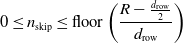 \begin{equation} 0 \leq n_{\text{skip}} \leq \text{floor}\left(\frac{R-\frac{d_{\text{row}}}{2}}{d_{\text{row}}}\right) \end{equation}
where $R$
is the effective range of the LiDAR and describes the maximum range at which acceptable spatial resolution is still achievable. In essence,
$R$
is the effective range of the LiDAR and describes the maximum range at which acceptable spatial resolution is still achievable. In essence, $n_{\text{skip}}$
acts as a tuning factor between survey speed and required point density, with larger values producing faster surveys at the expense of lower point densities. Since no prior information is known about the environment, any
$n_{\text{skip}}$
acts as a tuning factor between survey speed and required point density, with larger values producing faster surveys at the expense of lower point densities. Since no prior information is known about the environment, any $n_{\text{skip}} \gt 1$
may produce surveys with incomplete coverage. However, occlusion is likely not an issue if a traversable survey path exists, as this implies that sufficient space for the LiDAR to perceive the environment is present.
$n_{\text{skip}} \gt 1$
may produce surveys with incomplete coverage. However, occlusion is likely not an issue if a traversable survey path exists, as this implies that sufficient space for the LiDAR to perceive the environment is present.
5. Low-fidelity simulation
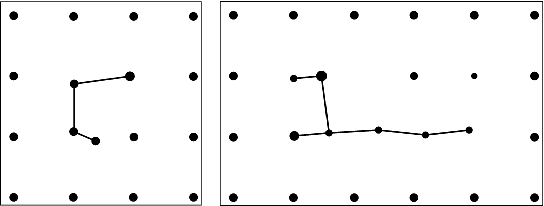
A low-fidelity simulation is used initially to evaluate potential performance differences between the three proposed variations. A purely 2D environment is used, and only UAV point positions are considered to reduce iteration times. For these tests, 100 random forest environments were generated and decomposed into obstacle primitives consisting of three or more stems joined by blockages. Blockages between adjacent trees are generated and the sum of maximum branch lengths between the two trees is greater than the distance between them. The remainder of the space is filled with regularly sized and spaced cylinders to maintain consistency between samples. Examples of obstacle primitives are in Fig. 8, where each is treated as an environment for which the navigation method is tasked to explore fully. A total of 164 obstacle primitives are used in this study. Travel distance is used as the metric for evaluating performance. To prevent the method from gaining excessive information regarding the small environment at the start, the sensor range for these tests is limited to 6 m with an angular resolution of 1 $^{\circ }$
.
$^{\circ }$
.
Top down view of two obstacle primitives used with the low fidelity simulator.
5.1. Performance
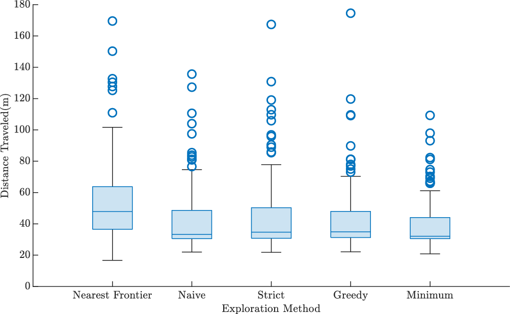
Each of the methods is used to explore around all obstacle primitives fully to examine relative performance between the three proposed methods. For comparison, results from the classic frontier exploration method [Reference Yamauchi16] are included. Each method is used to explore every test environment a second time with the full environment initially known to the path planner to produce a minimum path length for comparison. The minimum distance traveled for each environment out of all four methods is collated into a single set to serve as the theoretical minimum.
Looking first at the spread of distances traveled for each obstacle primitive in Fig. 9, the classic frontier method has the largest spread. Within the three proposed methods, the Greedy method has one test case which exceeds the maximum distance traveled of any other method. However, the remainder of the test cases performs better than all other methods. There is one single test case where classic frontiers outperform all the other methods with a very small travel distance, likely due to the extremely small survey area. Practically, a survey as small as this sample will never be conducted; therefore, this sample can be safely ignored. From inspection of the mean distance traveled for this set of obstacle primitives, it is immediately evident that the proposed method produces a travel distance advantage over classic frontiers, with a reduction in mean distance traveled between 18% with the Strict method and 22% with the method when compared to classic frontiers. While the Greedy method achieved the lowest mean distance traveled out of the three methods, the difference in mean between the best and worst-performing methods is 2.2∼m or approximately 5% of the worst-performing result. This suggests that while our methods appear to outperform classic frontiers, a higher fidelity simulation is required to determine which of the three methods provides maximum performance.
Boxplot of travel distances for each tested method. The minimum set is generated by rerunning all planners with the entire map visible and picking the minimum distance traveled for all primitives.
6. High-fidelity simulation
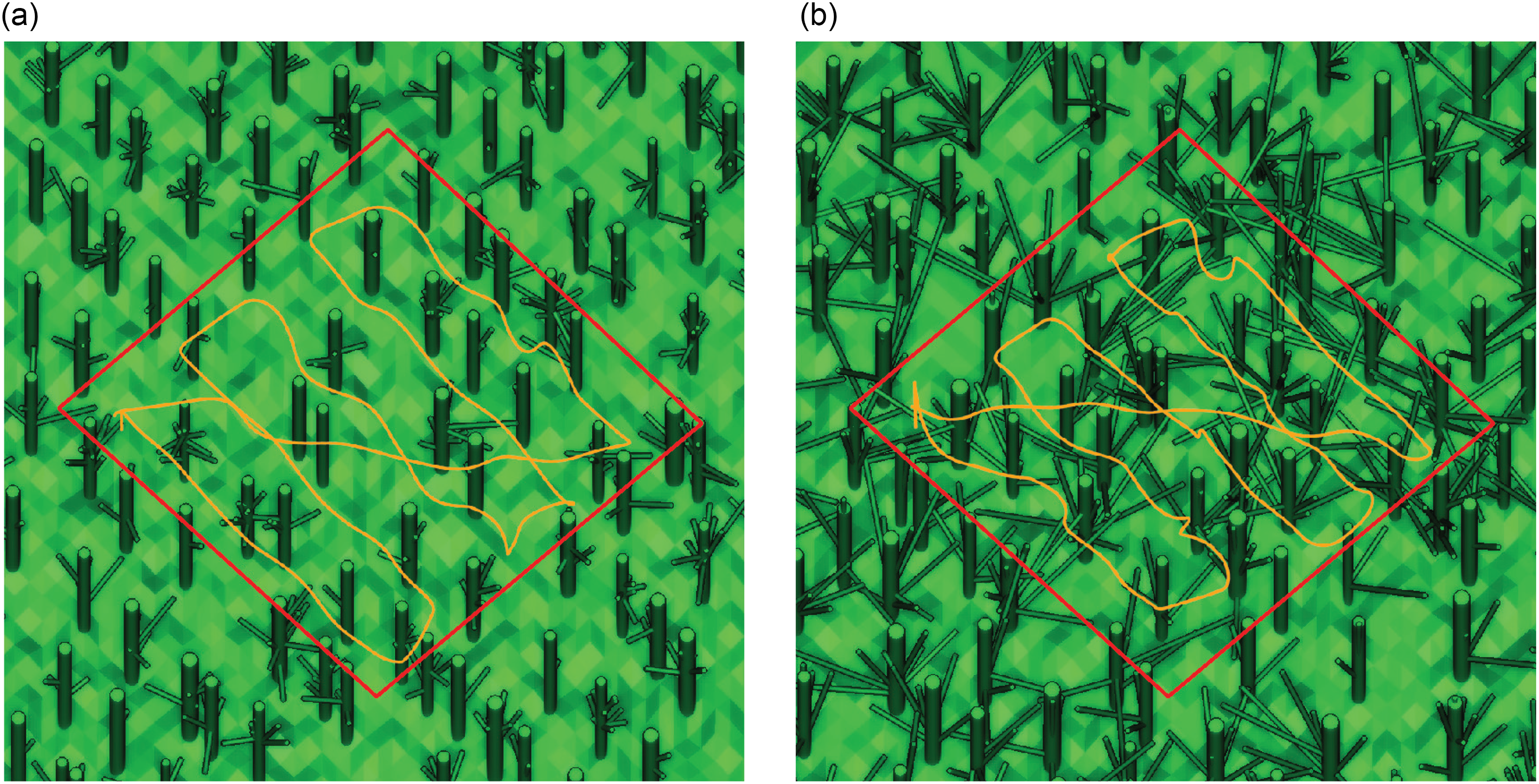
As the three presented methods have a marginal difference in measured travel distance, a full 3D simulation must be performed to determine performance. Two randomly generated environments are used for these tests to replicate areas with low and high branch density, shown in Fig. 10(a) and 10(b), respectively, using the parameters outlined in Table I. These environments are selected to represent the expected minimum and maximum difficulty in a traversable environment. While no full blockages exist along each traversed row, the presence of more branching in the high branch density environment generally produces less consistent surveys due to more changes in travel direction being required to avoid collisions. As sensing and variations in terrain are outside of the scope of this work, these two test environments represent two of the expected extremes; the first representing an unimpeded environment, and the second showing a more complex environment. To determine if there are performance benefits from the proposed methods, survey time and coverage information are compared against two state-of-the-art planners, FUEL [Reference Zhou, Zhang, Chen and Shen1], and Rapid Frontier [Reference Cieslewski, Kaufmann and Scaramuzza2].
Isometric views of (a) low and (b) high branching environments. The overall survey area is shown in red, and a sample path taken for a full survey is overlaid in orange.
6.1. Experiment setup
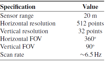
Because exploration performance is heavily affected by the employed motion planner, all experiments are conducted using the same trajectory planner and simulation setup in ref. [Reference Zhou, Zhang, Chen and Shen1]. Since omnidirectional LiDAR is generally preferred over RGB-D or narrow FOV LiDAR sensors for plantation forest surveys, the simulated depth camera is instead replaced with an omnidirectional LiDAR replicating specifications of an Ouster OS0-32. The relevant specifications of the simulated LiDAR are outlined in Table II. For each experiment, the UAV is initially placed between two rows, then tasked to explore 20 m down five rows for a survey area of approximately 22 by 22 m, representing the minimum viable survey area for a plantation forest. Once the environment is fully explored, the UAV is tasked to return to the starting position. Since the sensor range exceeds the distance between rows, the Naive and Strict methods are tested at both $n_{\text{skip}} = 0$
and
$n_{\text{skip}} = 0$
and $n_{\text{skip}} = 1$
. Lastly, each method is run 10 times at maximum velocities of 1, 2, and 3 m/s to examine performance scaling with higher survey speeds. Because the rate of information gain is fixed by the sensor used, the increase in target survey velocities will examine the optimality of each waypoint selection method with reduced environmental information.
$n_{\text{skip}} = 1$
. Lastly, each method is run 10 times at maximum velocities of 1, 2, and 3 m/s to examine performance scaling with higher survey speeds. Because the rate of information gain is fixed by the sensor used, the increase in target survey velocities will examine the optimality of each waypoint selection method with reduced environmental information.
Summary of specifications of simulated LiDAR sensor.
6.2. Survey time and distance traveled
The first series of results examines the survey time for each tested method, consisting of the time taken to complete the entire survey, then return to the starting position. Survey times for the two environments are shown in Fig. 11.
Survey completion time for (Top) low and (Bottom) high branching environments at tested velocities. Note the significantly reduced spread of the Naive and Strict methods compared to the two tested generalized exploration methods.
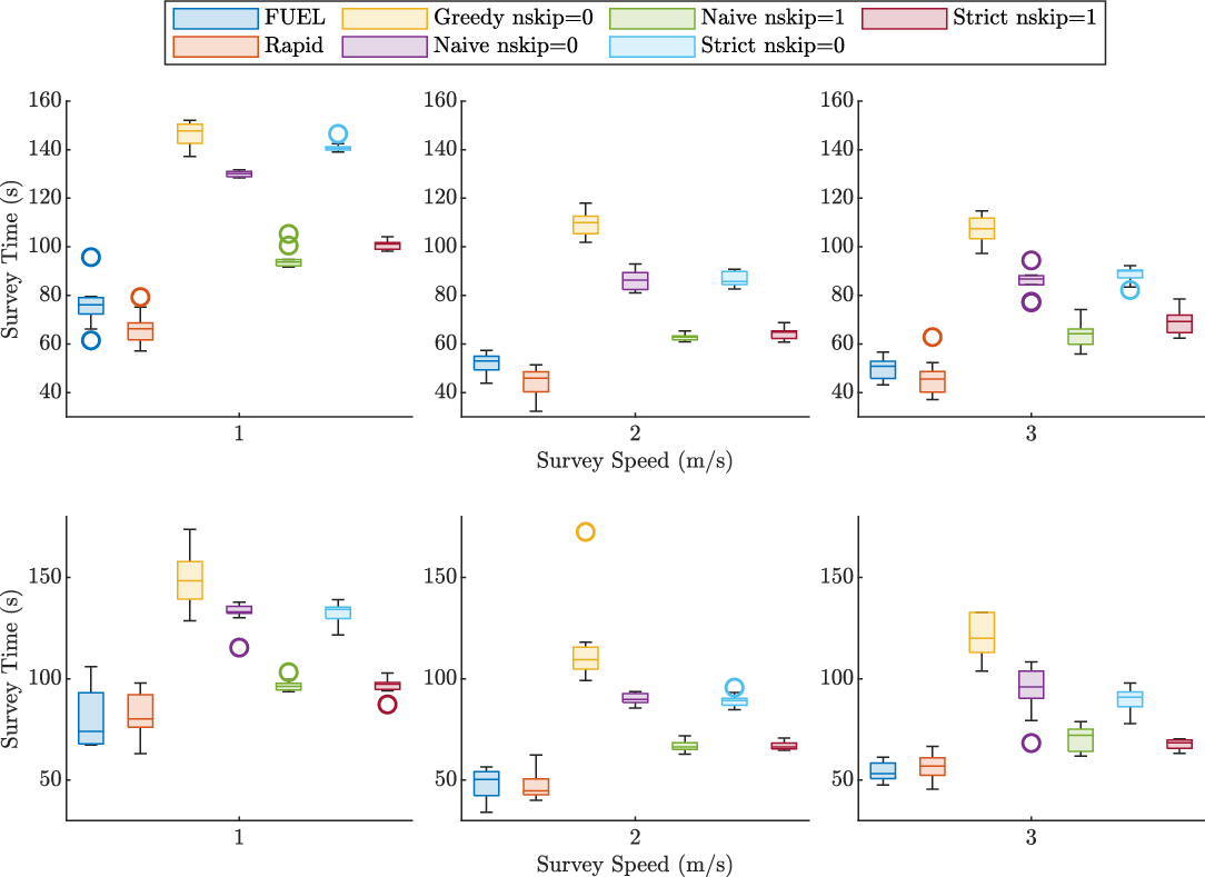
All methods in both environments produced a reduction in survey time by between 25% and 44% when the survey speed increased from 1 to 2 m/s. However, no significant improvements are observed when moving from 2 to 3 m/s. Increasing the maximum survey speed up to 3 m/s almost always results in increased survey time compared to the same method at 2 m/s, the maximum increase being 27% in the case of Rapid Frontiers on the high branching environment. The decrease in performance at 3 m/s is likely a result of dynamic limits imposed by the trajectory planner. Rapid Frontiers provided the shortest exploration time at all tested speeds, likely owing to omnidirectional sensing allowing the UAV to traverse for long periods in a single direction. Unexpectedly, the Greedy method performs the worst, with the spread in survey time being as large as the generalized exploration methods while also producing significantly longer surveys. This increase in survey time is likely due to the closest waypoint heuristic guiding the UAV towards close but dynamically expensive waypoints, leading to increased survey time.
Summary of survey time results at 2 m/s, lower is better.
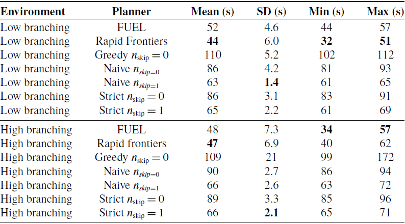
Bold values indicate the best performing method for each metric.
Distance traveled versus survey time for (a) low and (b) high branching environments. Dotted lines show a line of best fit for all trials conducted at their respective speeds.

The Naive and Strict methods both produce very consistent survey times, with slight run-to-runALS variation compared to the Greedy and generalized exploration methods. This can be seen by looking at the results at a survey speed of 2 m/s as shown in Table III. The Naive method with $n_{\text{skip}} = 1$
on the low-branching environment produces a 69% or 76% reduction in survey time standard deviation compared to FUEL and Rapid Frontiers, respectively. In the high-branching environment, the Strict method with
$n_{\text{skip}} = 1$
on the low-branching environment produces a 69% or 76% reduction in survey time standard deviation compared to FUEL and Rapid Frontiers, respectively. In the high-branching environment, the Strict method with $n_{\text{skip}} = 1$
produces a 71% or 69% reduction in survey time standard deviation compared to FUEL and Rapid Frontiers. However, this corresponding decrease in standard deviation also increases the mean sample time by between 23% and 45% from the overall longer travel path. This suggests that the proposed methods do not reduce the time taken for a full survey, but the followed trajectories vary less between different surveys. This increase in consistency will aid forestry surveys during the planning stage, as more consistent flight times allow for better planning of available energy.
$n_{\text{skip}} = 1$
produces a 71% or 69% reduction in survey time standard deviation compared to FUEL and Rapid Frontiers. However, this corresponding decrease in standard deviation also increases the mean sample time by between 23% and 45% from the overall longer travel path. This suggests that the proposed methods do not reduce the time taken for a full survey, but the followed trajectories vary less between different surveys. This increase in consistency will aid forestry surveys during the planning stage, as more consistent flight times allow for better planning of available energy.
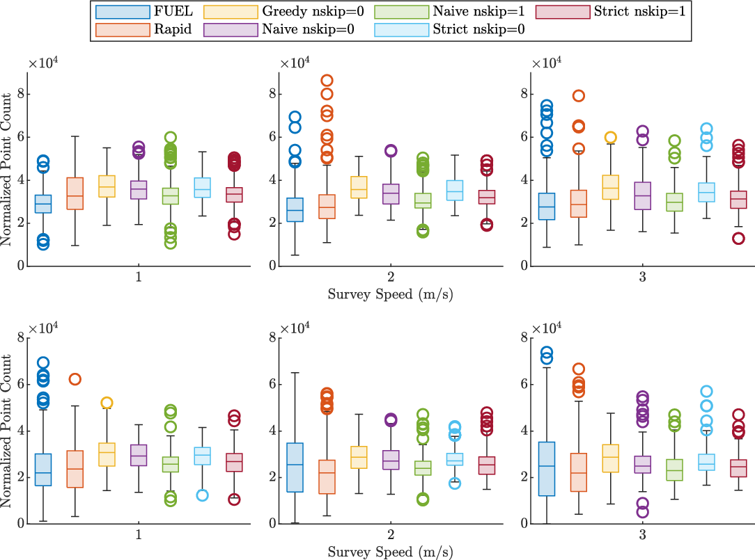
Normalized point count around each tree for (top) low and (bottom) high branching environments.
Normalized point count at each tree within the high-branching environment for each tested method. Each dot indicates the location of a specific tree stem. Points with a blue hue indicate lower point density, while points with a green hue indicate high density. Path taken during each experiment is shown as the blue line. Nonuniformity is shown as the difference in hue between points.

An expected increase in distance traveled with increasing sample time is shown for all tested scenarios when looking at the distance traveled versus survey time metrics in Fig. 12. In general, the results can be clustered into two groups: the first consisting of samples collected at a maximum survey speed of 1 m/s and the second consisting of those surveyed at 2 and 3 m/s. The trend lines for samples surveyed at 2 and 3 m/s are relatively similar, with the gradient of the trend line at 3 m/s slightly lower than that of the 2 m/s sample, producing a reduction in survey performance at the higher velocity. This suggests that the UAV or trajectory planner is exceeding dynamic limits at a maximum velocity of 3 m/s for the tested method and producing frequent start/stop events reducing the average velocity of the survey. Interestingly, the Strict and Naive methods produce mostly higher velocity surveys only when $n_{\text{skip}} = 0$
, which most samples being above the trend line, while the samples are more evenly distributed when
$n_{\text{skip}} = 0$
, which most samples being above the trend line, while the samples are more evenly distributed when $n_{\text{skip}} = 1$
. The Greedy method generally produces slower than average surveys for all tested cases.
$n_{\text{skip}} = 1$
. The Greedy method generally produces slower than average surveys for all tested cases.
6.3. Coverage
Coverage is defined as the number of points within a 0.5-m radius around each tree position, normalized to a survey time of 100 s for this series of tests. This process is completed since the number of acquired points around each tree is directly correlated to the sensor data rate and survey time. Since methods producing longer flights naturally acquire more points from the sensor, not normalizing the number of points to the sample time would result in a heavy skew in favor of slower methods as opposed to methods that utilize sample time more effectively. The point density per tree value can be thought of as a rate of information gain—higher values indicate the associated method is producing more observations per unit time, therefore surveying in a much more efficient manner. The normalized point count distribution for each tested method is shown in Fig. 13.
Visual inspection shows that an increase in survey speed does not significantly influence the mean coverage efficiency of the tested methods. In general, the mean coverage for the proposed methods is higher, which implies that the structured exploration approaches produce more useful points per unit of time. The exception to this is the high-branching case at survey speeds at 2 m/s or higher, where comparable mean normalized coverage between FUEL and the proposed methods is observed. However, FUEL fails to sufficiently observe every tree in the high-branching environment, likely due to occlusion. For the generalized methods, the increase in survey speed also increases the spread of coverage, with higher speeds producing a noticeably higher spread. This effect is particularly pronounced with the low branching test environment, where an increased spread of approximately 30%–40% is observed between survey speeds of 1 and 2 m/s. However, the range of coverage for the three proposed methods remains approximately the same regardless of the survey speed, further reinforcing the consistency versus survey time tradeoff.
The large spread of point densities in the generalized exploration methods can be explained by observing the spatial distribution of densities during the survey. Figure 14 shows the flight path and point density distribution in the complex environment at 2 m/s for each tested method. As the goal is to investigate the distribution of densities, each sample is normalized to the tree of maximum point density in the sample. FUEL and Rapid Frontiers, both shown in Fig. 14(a) and 14(b), respectively, show a path that does not visit the entire region of interest. Instead, regions are marked as explored as soon as there are sensor observations in the region. This results in both less time spent observing these regions and any observations containing fewer points due to point spacing at long range, resulting in significantly reduced point density around these regions. In contrast, the structured exploration approaches are forced to visit the entire region of interest, resulting in better consistency of samples. The effect of this consistency can be seen in Table IV, which illustrates the parameters of the median point density trial for all tested methods. In both environments, structured exploration approaches provided higher mean point counts when compared to the generalized methods. The structured exploration approaches reduced point density standard deviation between 56% and 75% when compared to FUEL and 39% to 65% when compared to Rapid frontiers. In direct contrast to survey time results, the Greedy method offered both the highest mean normalized point density and the lowest standard deviation despite producing the longest surveys, followed by the Strict, and finally the Naive method. The increase in $n_{\text{skip}}$
produces a corresponding increase in density spread due to trees being observed from a longer range.
$n_{\text{skip}}$
produces a corresponding increase in density spread due to trees being observed from a longer range.
Summary of normalized point density at 2 m/s for median point density test cases.
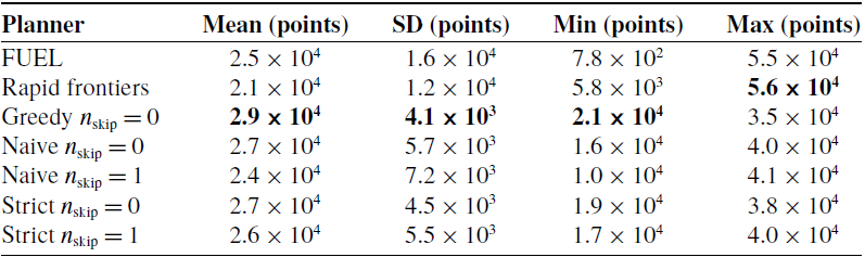
Bold values indicate the best performing method for each metric.
Test site used for testing of the Strict method.
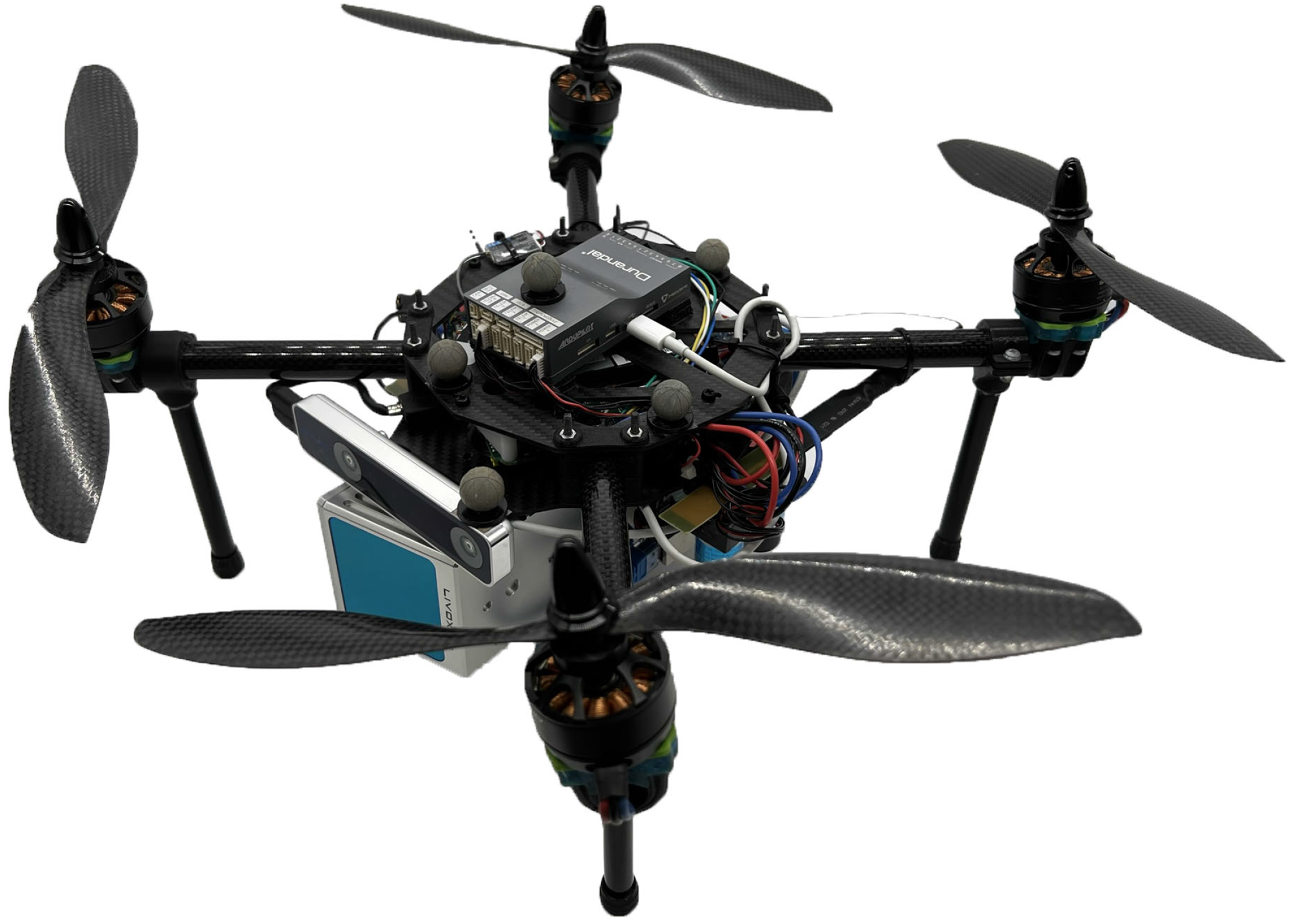
UAV used for flight tests. The payload consists of an Intel NUC, a Livox MID-70, and an Intel Realsense T265.
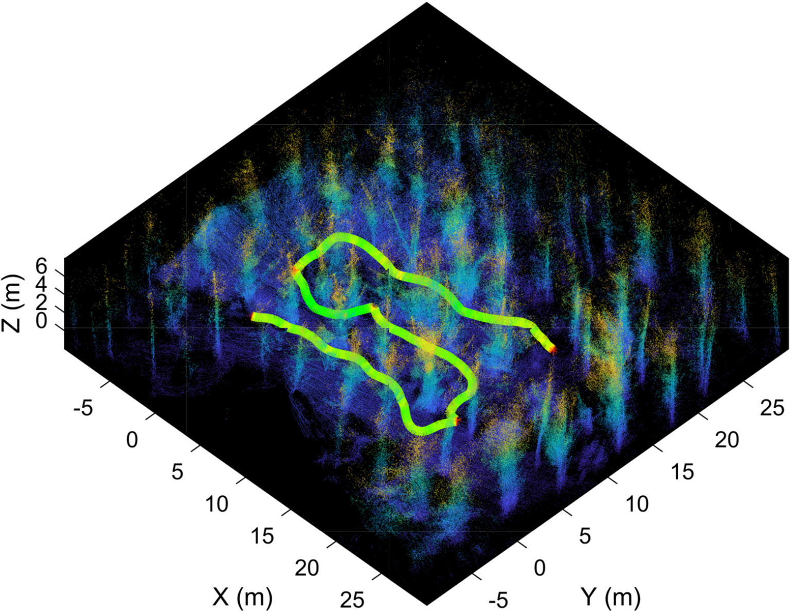
Downsampled point cloud capture of flight test. The survey area is approximately 22 by 15 m. The flight path taken is shown as a color-coded line. Green hues indicate faster travel speeds, while red hues indicate slower speeds.
7. Flight experiments
Finally, a one-shot trial is conducted on a plantation located in Riverhead Forest, Auckland, New Zealand as a preliminary test for the proposed method. This aims to determine if simple waypoint placement in the Strict method is sufficient to fully navigate the environment; therefore, coverage and survey time metrics will not be evaluated. The environment consists of an unpruned forest with eight approximately parallel rows, little undergrowth, and relatively flat terrain. The first row of the flight environment is shown in Fig. 15, showing the presence of a flight corridor with some low-hanging branches. The flown UAV, shown in Fig. 16, consists of a standard quadrotor carrying an Intel NUC, a Livox MID-70 LiDAR, and an Intel Realsense T265 camera. Flight control is accomplished using a Holybro Durandal flight controller running PX4 1.12.3. As there is no globally consistent source of pose information within the forest, R3Live [Reference Lin and Zhang42] is used for state estimation, and depth data is provided by a Livox MID-70 LiDAR. All processing is carried out on the onboard NUC with trajectory generation using our constant speed trajectory planner and the trajectory follower outlined in ref. [Reference Lin and Stol43]. The choice of a narrow FOV LiDAR over the simulated wide FOV LiDAR is mainly due to the availability and cost constraints of wide FOV sensors. However, since the waypoints are pre-placed in this trial, effects on performance will be restricted to a change in the density of the resulting point cloud.
In this test, the UAV is tasked to traverse three corridors using the Strict method with $n_{\text{skip}} = 0$
, forming a survey area of approximately 22 by 15 m. Figure 17 shows a downsampled point cloud of the environment captured during flight and the flown flight path. This flight test demonstrates a successful application of the Strict method within a complex, uncontrolled environment.
$n_{\text{skip}} = 0$
, forming a survey area of approximately 22 by 15 m. Figure 17 shows a downsampled point cloud of the environment captured during flight and the flown flight path. This flight test demonstrates a successful application of the Strict method within a complex, uncontrolled environment.
8. Conclusions
This paper presents structured approaches for autonomous exploration within plantation forest environments using multirotor UAVs to produce higher-quality surveys. The proposed method uses a two-tiered approach, where waypoints are placed according to a lawnmowing pattern, and a trajectory planner is employed to produce the executed trajectory. Simulation testing using procedurally generated plantation forest environments is used to evaluate the proposed methods’ performance, which produced improved point density within the region of interest at the expense of longer surveys. Finally, one of the proposed methods is used to explore a section of an actual plantation forest to demonstrate functionality. As this paper only details the waypoint selection process, future work will be focussed on adaptive waypoint selection based on identifying the rows present in the environment to enable fully autonomous survey flights within plantation forests.
Author Contributions
Tzu-Jui Lin and Karl A. Stol conceived and designed the study, Tzu-Jui Lin carried out the experiment, data analysis, and wrote the initial manuscript. All authors contributed critically to the draft manuscript and gave final approval for publication.
Financial Support
The lead author is supported by a University of Auckland Doctoral Scholarship.
Conflicts of Interest
The authors declare that they have no conflicts of interest.
Ethical Considerations
This article does not contain any studies with human or animal participants.


 Open access