





Non-technical Summary
It has long been wondered whether space and time influence ecosystems in similar ways. This idea, known as space–time equivalence, suggests that ecological change seen across space at any given time is analogous to the change seen across time in any given space. We tested whether space–time equivalence is observed in the fossil mammal community structures of western Europe throughout the warm stages of the Pleistocene. We showed that evidence for space–time equivalence was present in the most species-rich functional group of mammals. In less species-rich groups, there was strong evidence to suggest that space–time equivalence did not hold. We propose that this is because less species-rich functional groups are more sensitive to climatic changes, which disproportionately disrupted their ecological patterns of assembly when compared with the richest group. Our findings suggest that space–time equivalence may therefore only be assumed in certain subsets of mammal communities or more generally in regions with less dramatic climatic changes.
Introduction
The idea that time and space are not independent in their effects on ecological community assembly has long been suggested in the absence of a formalized, conceptual framework (Preston Reference Preston1960). The idea is implicitly assumed in any application that extrapolates present spatial relationships to derive information about the past or future. Given the decreasing temporal scale of most ecological studies (Estes et al. Reference Estes, Elsen, Treuer, Ahmed, Caylor, Chang, Choi and Ellis2018), space-for-time substitutions (Pickett Reference Pickett and Likens1989) are becoming an increasingly useful (e.g., Banet and Trexler Reference Banet and Trexler2013; Blois et al. Reference Blois, Williams, Fitzpatrick, Jackson and Ferrier2013; Wogan and Wang Reference Wogan and Wang2017; Lovell et al. Reference Lovell, Collins, Martin, Pigot and Phillimore2023), but criticized (Damgaard Reference Damgaard2019) tool for understanding long-term changes in ecosystems. Despite the prevalence of space-for-time substitution studies, there are few that explicitly test this relationship (but see Blois et al. [Reference Blois, Williams, Fitzpatrick, Jackson and Ferrier2013] for a notable exception), and even fewer generalized models that directly and quantitatively underpin the concept of space–time equivalence.
Perhaps the most recognized development of a quantitative, unified space–time relationship in ecology is the species–time–area relationship (STAR; Adler and Lauenroth Reference Adler and Lauenroth2003; Adler et al. Reference Adler, White, Lauenroth, Kaufman, Rassweiler and Rusak2005), which combined the species–area relationship (SAR) and the species–time relationship (STR). Both the SAR and STR independently show a scale dependence on species accumulation (Preston Reference Preston1960). In both modern (Adler et al. Reference Adler, White, Lauenroth, Kaufman, Rassweiler and Rusak2005) and fossil (Raia et al. Reference Raia, Carotenuto, Meloro, Piras and Barbera2010; Du and Behrensmeyer Reference Du and Behrensmeyer2018) contexts, the larger the sample space or sample time, the greater the species richness. Conjectured equivalence between spatial and temporal rates of accumulation suggests that time and space could be considered interchangeable in their effects on diversity (Rosenzweig Reference Rosenzweig, McKinney and Drake2001).
Fossil community structures may likewise exhibit a predictable relationship between time and distance across similar environmental trajectories (Louys et al. Reference Louys, Price and Travouillon2021). Equivalence between community structure in time and space was suggested for mammal communities in Southern Australia, with 1000 years in time equivalent to ~925 km in space, although this specific example has yet to be generalized. Nevertheless, these quantitative approaches support the suggestion that ecological assemblies exhibit ergodicity (Herben et al. Reference Herben, During, Law, Dieckmann, Law and Metz2000; Rosenzweig Reference Rosenzweig, McKinney and Drake2001). Ergodicity originates from statistical mechanics (Boltzmann Reference Boltzmann1884, Reference Boltzmann and Brush1964; Gallavotti Reference Gallavotti1995) and describes an equivalence between the ensemble average—the average over space at a fixed time—and the time average—the average at a fixed space over time (Szász Reference Szász and Szász2000). Relating this concept to community ecology would suggest an equivalence between community richness or structure over space and time (Rosenzweig Reference Rosenzweig, McKinney and Drake2001), although the time component provided by modern ecological studies generally precludes quantitative examination of this phenomenon (Herben et al. Reference Herben, During, Law, Dieckmann, Law and Metz2000).
Community convergence (Fuentes Reference Fuentes1976; Andrews et al. Reference Andrews, Lord and Evans1979) should guarantee ergodicity when an environment is entirely homogeneous over space and time. Where environmental heterogeneity exists in an area, a spatial average can be calculated to represent the multiple communities inhabiting these environments. Should spatial heterogeneity be stable over time, or return periodically, the difference between temporal and spatial averages should be distributed symmetrically about zero. This symmetry does not wholly validate space-for-time substitution (Pickett Reference Pickett and Likens1989), which suggests that spatial patterns of any single time slice represent the temporal trajectory of any given space. Rather, it suggests that over the entire system, spatial and temporal averages converge. Here, we use a community structure framework that can be applied to fossil remains to provide the time depth necessary to test ergodicity. Specifically, we test whether mammal community structures in Pleistocene western Europe are ergodic as predicted by space–time equivalence models.
Materials and Methods
Fossil Data
We restricted our analyses to fossil mammalian fauna, with volant and aquatic mammals omitted due to taphonomic and representational biases in community structure analysis (Wallgren Reference Wallgren2008; Muldoon and Goodman Reference Muldoon and Goodman2010; Lintulaakso and Kovarovic Reference Lintulaakso, Kovarovic, Casanovas-Vilar, van den Hoek Ostende, Janis and Saarinen2023). Published information on fossil occurrences across sites in western Europe (Supplementary Table S1) were used to construct a presence–absence matrix. We assigned each taxon to an ecological guild following Louys et al. (Reference Louys, Meloro, Elton, Ditchfield and Bishop2011), excepting body mass, for which we consider only two categories: small (<10 kg) and large (≥10 kg). Taphonomic biases in our chosen sites and operational constraints of our analyses preclude finer parsing of body mass. Thus, we consider here up to eight guilds: small terrestrial primary consumers (STP), large terrestrial primary consumers (LTP), small terrestrial secondary consumers (STS), large terrestrial secondary consumers (LTS), small arboreal primary consumers (SAP), large arboreal primary consumers (LAP), small arboreal secondary consumers (SAS), and large arboreal secondary consumers (LAS) (Supplementary Table S2).
For extant taxa, guild assignment follows Louys et al. (Reference Louys, Meloro, Elton, Ditchfield and Bishop2015). Where an extant taxon was not assigned, guilds were based on descriptions by Mittermeier et al. (Reference Mittermeier, Rylands and Wilson2013), Wilson et al. (Reference Wilson, Mittermeier and Lacher2016, Reference Wilson, Mittermeier and Lacher2017), and Wilson and Mittermeier (Reference Wilson and Mittermeier2009, Reference Wilson and Mittermeier2011, Reference Wilson and Mittermeier2018). Following Louys et al. (Reference Louys, Meloro, Elton, Ditchfield and Bishop2015), we apply terrestrial and primary consumer labels conservatively; that is, only when evidence for observed or reconstructed arboreal behavior or secondary consumption was absent. This does not imply that any taxa were assigned as arboreal or secondary consumer by default, but rather that we employed a low threshold of evidence to assign taxa to these groups. Thus, we consider both omnivores and insectivores as secondary consumers. Similarly, we consider taxa as arboreal if either potential or strict arboreality is inferred. Taxa such as the porcupine (Hystrix) and wolverine (Gulo) are thus considered arboreal under this criterion, despite not usually being considered tree-dwelling species, due to their implied arboreal capability (e.g., Nowak Reference Nowak1999; Wright and Ernst Reference Wright and Ernst2004). For extinct fauna, body mass and dietary and locomotory adaptations were assigned based on published reconstructions. Where reconstructions were not available, guild assignments were based on comparisons with assigned taxa closest in morphology or phylogeny (Supplementary Table S2). Comparisons in functional morphology took precedence over phylogeny. Taxa resolved above the species level were assigned the most common trait of their constituent species. Community structures were then quantified by calculating the proportional representation of the guilds within each spatiotemporal interval.
We restricted our analyses to well-described fossil sites of Britain, France, Germany, the Netherlands, and Belgium in western Europe to limit latitudinal and altitudinal impacts on mammal community structure. Latitudinal constraints help ensure similar assembly rules and more uniform environmental control on community structure (Fleming Reference Fleming1973). We similarly excluded alpine localities, as elevation gradients appear to significantly alter community structure (Able and Noon Reference Able and Noon1976; Rickart Reference Rickart2001; McCain Reference McCain2007; Gámez and Harris Reference Gámez and Harris2022). The fossil communities used range from a single stratigraphic layer within one pit to multiple localities across a single fossiliferous region and were included if the published record suggests that the assemblage can be interpreted as a single community. Where available, exact coordinates representing each site’s location were used; however, where only hand-drawn maps or broad geographic descriptions were available, coordinates were approximated based on correlation between identified features documented in site descriptions and satellite imagery (Google LLC 2024). Each fossil community was assigned to a biogeographic region based on its spatial coordinates (European Environment Agency [EEA] 2016). Site-specific information can be found in Supplementary Table S1.
Ages associated with each assemblage were recorded as direct (e.g., radiometric dating) or indirect (e.g., biostratigraphy), with each assemblage assigned to a Marine Isotope Stage (MIS) based on the most parsimonious age estimates available (Supplementary Table S1). We limited our analyses to warm (odd-numbered) MISs, as much of our study area would have been under glaciers during glacial conditions or is now underwater. We use MIS 3 (57–29 ka), 5 (130–71 ka), 7 (243–191 ka), 9 (337–300 ka), and 11 (424–374 ka) following chronology provided by Lisiecki and Raymo (Reference Lisiecki and Raymo2005). While our analyses ignore any community state changes associated with movement into and out of glacial conditions, this allows us to compare community structures across the same broad environmental conditions. We used an upper bound of MIS 11, as sites within our study region have depositional periods unresolved to a single MIS beyond this point. We used a lower temporal bound of MIS 3, marking the final odd MIS of the Pleistocene.
Analysis
Fossil site data, presence–absence faunal lists, and guild assignments were imported into Jupyter Notebooks (Python v. 3.11.7). Sites were binned into spatial groups using two methods. The first used existing biogeographic zones to assign each fossil site a spatial group. Biogeographic regions have been shown to delineate boundaries where mammalian community structures are more similar within than between units (Rodríguez et al. Reference Rodríguez, Hortal and Nieto2006). We used the 11 delineations of the biogeographic regions in the EEA biogeographic map (2016), which represents a reclassification and generalization of natural vegetation (Roekaerts Reference Roekaerts2002; EEA 2006). Markova and Puzachenko (Reference Markova and Puzachenko2021) note the EEA’s biogeographic regions coincide closely with their qualitative mammalian bioregions of Europe (Markova and Puzachenko Reference Markova and Puzachenko2018; Puzachenko and Markova Reference Puzachenko and Markova2019), providing support for the use of the EEA vegetation maps as realistic natural zoogeographic divisions. GIS analysis (to assign biogeographic regions to fossil sites and visualize the study region) was conducted in Python using the Matplotlib (v. 3.8.0; Hunter Reference Hunter2007), Shapely (v. 2.0.4; Gillies et al. Reference Gillies, van der Wel, van den Bossche, Taves, Arnott and Ward2024), Geopandas (v. 1.0.1; van den Bossche et al. Reference Van den Bossche, Jordahl, Fleischmann, Richards, McBride, Wasserman and Badaracco2024), and Cartopy (v. 0.22.0; Met Office 2023) packages.
We also examined natural spatial grouping in our locality dataset using the Density-Based Spatial Clusters of Applications with Noise (DBSCAN) algorithm (Ester et al. Reference Ester, Kriegel, Sander, Xu, Simoudis, Han and Fayyad1996). This technique can spatially cluster points of arbitrary shapes such as those represented by fossil sites from a search radius (ε) and minimum number of points (minPts). The algorithm was implemented using Scikit-learn (v. 1.2.2) on longitude and latitude using the haversine metric to appropriately approximate the distance between points on the surface of a sphere (Pedregosa et al. Reference Pedregosa, Varoquaux, Gramfort, Michel, Thirion, Grisel and Blondel2011). The essential parameters were manually tuned to ε = 0.02 and minPts = 6; reflecting the mammalian biogeographic regionalizations between Britain and mainland Europe observed by Heikinheimo et al. (Reference Heikinheimo, Fortelius, Eronen and Mannila2007) and Markova and Puzachenko (Reference Markova and Puzachenko2018).
We ran our analyses using three separate methods of spatial binning: (1) the EEA (2016) biogeographic regions; (2) DBSCAN clustering; and (3) a mixed approach, consisting of DBSCAN clusters within EEA biogeographic regions. Fossil sites were assigned to space–time intervals based on their assigned MIS and spatial cluster, such that presence–absence could be aggregated across sites, defining spatially and temporally unique metacommunities. The total number of taxa representing the metacommunity at each space–time interval was counted (Supplementary Tables S3, S4, and S5), with intervals having fewer than 12 identified taxa omitted, the minimum threshold suggested to distinguish mixed and open-habitat types in fossil mammal assemblages (Louys et al. Reference Louys, Travouillon, Bassarova and Tong2009).
For each guild A, spatial averages 〈A〉 MIS were calculated as the mean proportional representation of A across all metacommunities at a fixed MIS (Fig. 1). Time averages Ā SPACE were calculated as the mean proportional representation of guild A across a single metacommunity over time in a fixed single spatial bin (Fig. 1). Ergodicity was examined by calculating the difference between the spatial and time averages (per guild) and determining whether that set of observed proximities was symmetric about the expected ergodic value of zero (Ā − 〈A〉 = 0). We used the nonparametric one-sampled Wilcoxon signed-rank test (Wilcoxon Reference Wilcoxon1945) to test the null hypothesis (H 0) that the median of the ergodic proximities (of each guild independently) equals zero. This was implemented in Python using Pingouin (v. 0.5.5; Vallat Reference Vallat2018) with the ergodic proximity arrays as the input.
Example time series highlighting the proportional representation of guild $ A $
across spatial clusters over Marine Isotope Stages (MIS) 11–3, with examples of time averaging, Ā—the averages constructed over time slices within a fixed spatial group—and spatial (ensemble) averaging, 〈A〉 – the averages constructed across spatial groups at a fixed time slice.
$ A $
across spatial clusters over Marine Isotope Stages (MIS) 11–3, with examples of time averaging, Ā—the averages constructed over time slices within a fixed spatial group—and spatial (ensemble) averaging, 〈A〉 – the averages constructed across spatial groups at a fixed time slice.

We avoid a sole reliance on p-values (Murtaugh Reference Murtaugh2014; Holland Reference Holland2019) and report the median and distribution (kernel density estimate) of ergodic proximities, associated p-values, and effect size (the matched-pairs rank-biserial correlation). The matched-pairs rank-biserial correlation shows the difference between the proportion of positive rank sums and the proportion of negative rank sums (Kerby Reference Kerby2014), highlighting the magnitude and direction that ergodic proximities stray from zero. We interpreted our results based on jackknife cross-validation, which provided confidence intervals to the median and effect size of our dataset (CI = (100 − α) %); and the frequency of p-values above and below α (sensitivity). Jackknife cross-validation was determined by iteratively removing an input from the analysis—specifically, ergodic proximity inputs for confidence intervals and space–time intervals for significant p-value counts. Decision rules to reject H 0 based on arbitrary significance thresholds (α) are reported to provide common values for refuting hypotheses, with arbitrary significance thresholds of 0.10, 0.05, and 0.01 selected as outlined in Hammer and Harper (Reference Hammer and Harper2024).
The null hypothesis, that ergodic proximities will center symmetrically around zero, implies a test against a random set of ergodic proximities, without accounting for the effects of our experimental design. Testing against a uniformly random set of ergodic proximities would produce uniformly distributed p-values, as the test statistic is equally likely to fall anywhere under the null. Simulating the experimental design under a uniformly random community assembly, however, will not test against this relationship, because the process of generating uniformly random inputs is ergodic itself. Random inputs into the experimental design will therefore rarely produce significant results. By scaling significance thresholds, our alternative hypothesis (H a) evaluates whether each guild deviates significantly from the expectation of a uniformly random ergodic process (the null model), where such deviations are expected by chance only 1%, 5%, or 10% of the time (corresponding to α = 0.01, 0.05, 0.10, respectively).
To determine appropriate scaling, a guild’s representation was randomly generated for the number of space–time intervals used in each experiment over 10,000 iterations. For each iteration, ergodic proximities were input into the Wilcoxon signed-rank test to determine the distributions (kernel density estimate) of p-values and effect sizes. We then compared these with a baseline distribution of p-values and effect sizes, determined from 10,000 uniformly random datasets (spanning the interval [−1, 1]). We adjusted our effect sizes based on a linear scaling factor, determined by matching the standard deviation of the effect size distribution from random ergodic proximities to that of the baseline distribution. Similarly, we adjust our significance thresholds (α = 0.10, 0.05, 0.01), based on the 10th, 5th, and 1st percentile of a numerical interpolation of the p-value distribution from random ergodic proximities.
Results
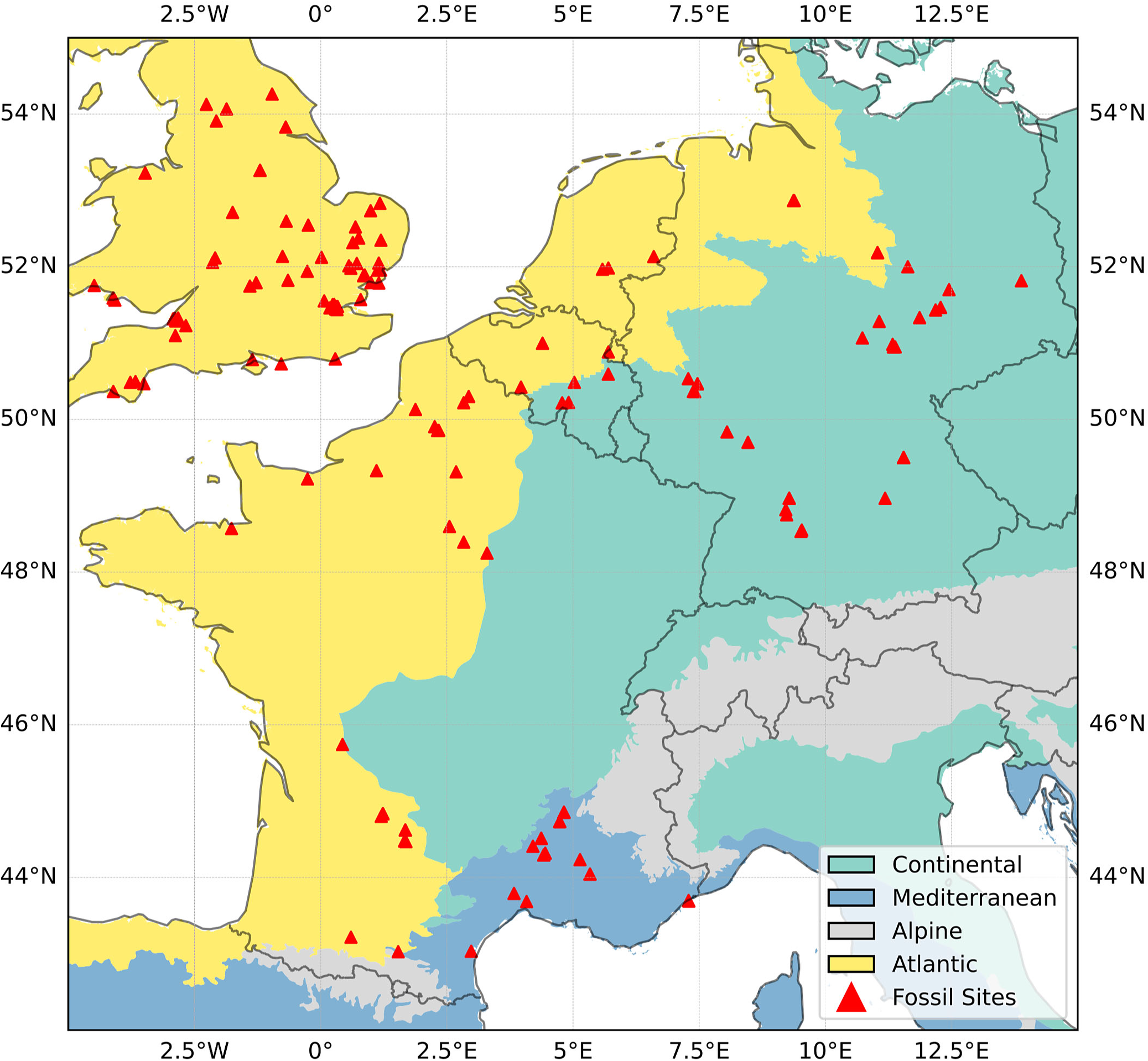
Communities from 163 assemblages (Fig. 2) were assigned to spatial clusters based on each clustering method, defining 3, 6, and 7 spatial groups for the biogeographic, DBSCAN, and mixed (biogeographic and DBSCAN) binning methods, respectively (Supplementary Figs. S1, S2, and S3). Extended results are documented in the Supplementary Material. For each spatial clustering method, the community structure over all valid space–time intervals is displayed as a discrete time series spanning five MISs (Supplementary Figs. S4, S5, and S6). Seven of the eight potential guilds were filled, with large arboreal primary consumers absent. Under biogeographic clustering (Supplementary Fig. S7), large arboreal and terrestrial secondary consumers significantly decreased with the sampling of taxa per bin (p < 0.10), while small terrestrial secondary consumers significantly increased (p < 0.05). With DBSCAN and mixed clustering (Supplementary Figs. S8 and S9), small arboreal primary consumers decreased significantly with the increased sampling of both sites per bin (p < 0.10) and taxa per bin (p < 0.05).
Study area of western Europe, with used fossil localities overlaid on the European Environment Agency (EEA 2016) biogeographic regions.
Our random simulations indicated that p-values gathered from analysis of biogeographic, DBSCAN, and mixed clustering methods should be compared with significance thresholds of 0.7437, 0.7169, and 0.7029, respectively, for α = 0.10; 0.6451, 0.6375, and 0.6201 for α = 0.05; or 0.4293, 0.4364, and 0.4118 for α = 0.01 (Supplementary Figs. S10, S11, and S12). Similarly, factors of 4.1704, 4.1246, and 3.9338 scaled the effect sizes retrieved from biogeographic, DBSCAN, and mixed clustering experiments, respectively (Supplementary Figs. S10, S11, and S12). While effect size spans the interval [−1, 1], adjusting the spread using linear scaling may amplify extreme unscaled effects outside of this range. Thus, scaled effects outside ±1 are interpreted as extreme.
The analyses using biogeographic clusters (Table 1, Supplementary Fig. S13) showed p-values supporting the null hypothesis of ergodicity in four of the seven occupied guilds, with significance present in large terrestrial primary consumers (at α = 0.10), small arboreal primary consumers (at α = 0.05), and small terrestrial primary consumers (at α = 0.01). The average confidence interval associated with the scaled effect sizes when using biogeographic clusters spans 1.302, highlighting an extreme degree of uncertainty. The direction of the effect is uncertain across all insignificant guilds and the large terrestrial primary consumer guild. The magnitude of the effect is also uncertain in small arboreal and terrestrial primary consumers with confidence intervals spanning [−1.5774, −0.3138] and [0.5607, 1.8399], respectively.
Outputs of Wilcoxon signed-rank tests on ergodic proximities
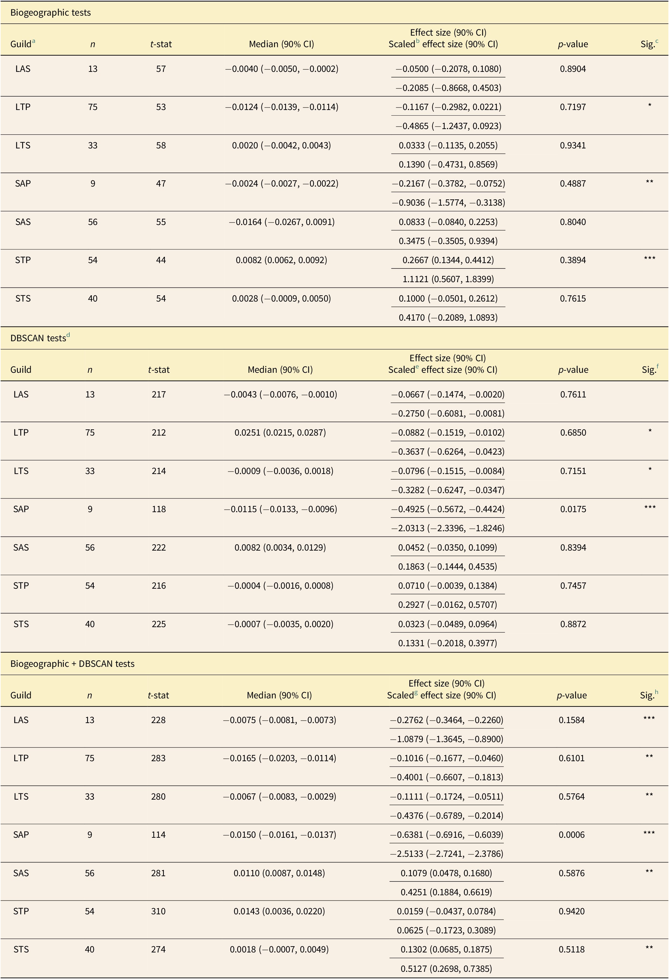
a Guild abbreviations: LAP, large arboreal primary consumers; LAS, large arboreal secondary consumers; LTP, large terrestrial primary consumers; LTS, large terrestrial secondary consumers; SAP, small arboreal primary consumers; SAS, small arboreal secondary consumers; STS, small terrestrial secondary consumers; STP, small terrestrial primary consumers.
b Effect scaling factor: 4.1704.
c Significance thresholds (Sig.): *α = 0.1→0.7437; **α = 0.05→0.6451; ***α = 0.01→0.4293.
d DBSCAN, Density-Based Spatial Clusters of Applications with Noise.
e Effect scaling factor: 4.1246.
f Significance thresholds (Sig.): *α = 0.10→0.7169; ***α=0.01→0.4365.
g Effect scaling factor: 3.9388.
h Significance thresholds (Sig.): **α = 0.05→0.6201; ***α = 0.01→0.4118.
The analyses using DBSCAN clusters (Table 1, Supplementary Fig. S14) showed significant p-values, refuting the null hypothesis in large terrestrial primary and secondary consumers (at α = 0.10), as well as in small arboreal primary consumers (at α = 0.01). This finding is supported by their respective moderate (−0.3637, −0.3282) and extreme (−2.0313) scaled effect sizes. Compared with biogeographic clustering, scaled effect sizes exhibit markedly reduced confidence intervals, spanning an average of 0.5819. The jackknife cross-validation (Supplementary Table S6) shows that both significant and insignificant guilds produce p-values occasionally fluctuating about the largest scaled significance threshold (α = 0.10), except for small arboreal primary consumers. Support for the alternative hypothesis was consistent in 13/24 (54% accuracy) and 12/24 (50% accuracy) jackknife resamples for large terrestrial primary and secondary consumers, respectively. However, the small arboreal primary consumer guild was significant in 24/24 (100% accuracy) resamples, even at the most conservative threshold (α = 0.01).
The analyses using the mixed (biogeographic and DBSCAN) clusters (Table 1, Supplementary Fig. S15) showed significant p-values in all guilds except small terrestrial primary consumers. Moderate effect sizes provide support for refuting the null hypothesis at the α = 0.05 threshold in large terrestrial primary and secondary consumers, and small arboreal and terrestrial secondary consumers (−0.4001 and −0.4376, and 0.4251, and 0.5127 respectively). Furthermore, extreme effect sizes support refuting the null hypothesis at the α = 0.01 threshold in large arboreal secondary consumers, and small arboreal primary consumers (−1.0879 and −2.5133 respectively). Using the mixed clustering approach reduced the average span of scaled effect size confidence intervals again, to 0.4572. This model was also shown to be the most robust when comparing significance (at α = 0.10) to jackknife resamples (Supplementary Table S6), with average accuracy of 84% compared with 71% in the other models. The insignificance of small terrestrial primary consumers was the most inconsistent (at α = 0.10), with support for the null hypothesis in 66% (16/24) of jackknife resamples (Supplementary Table S6). While this does not demonstrate that the ergodic proximities of small terrestrial primary consumers stray from ergodicity as much as those of other guilds, there is still uncertain support for the null hypothesis.
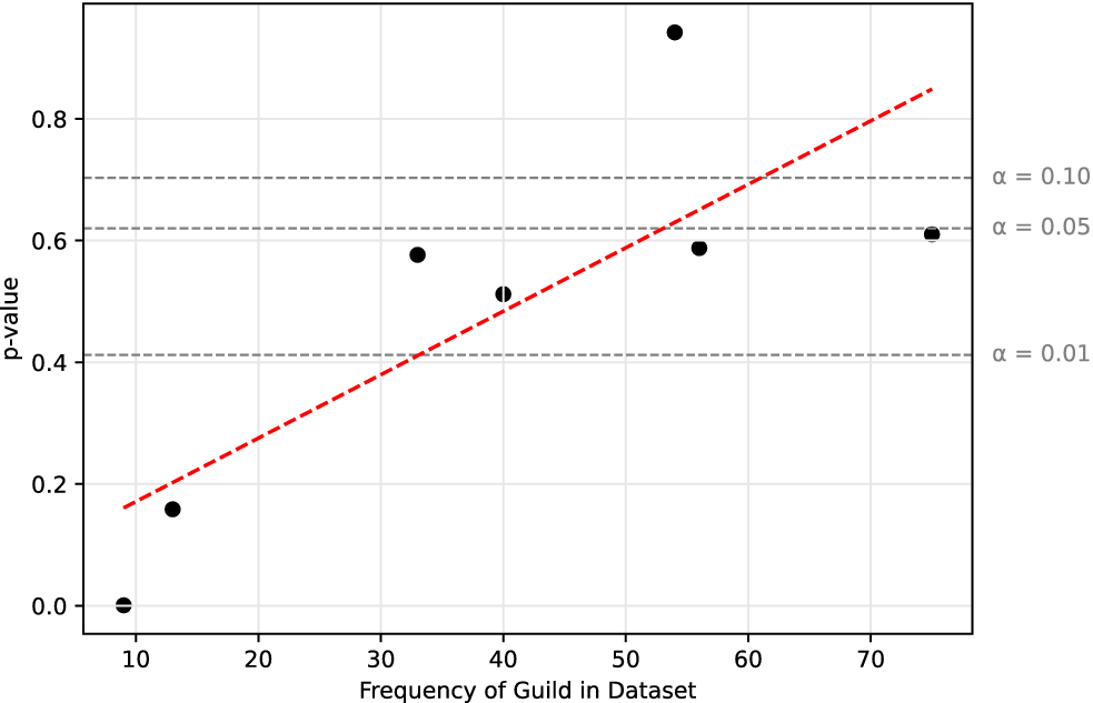
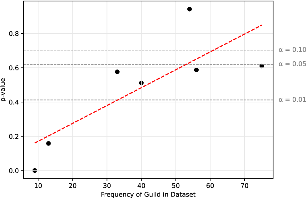
For biogeographic groups, there was an insignificant correlation between the richness of each guild (the number of taxa identified in it) and that guild’s p-value (Supplementary Fig. S16). This was also insignificant when using DBSCAN groups (Supplementary Fig. S17). The mixed (biogeographic and DBSCAN) model, however, showed a significant positive linear correlation (p < 0.05; Fig. 3). Rerunning each analysis using taxa only resolved to the species level showed a significant correlation in both the biogeographic and DBSCAN trials (Supplementary Figs. S18 and S19), but not the mixed (biogeographic and DBSCAN) model (Supplementary Fig. S20).
Significant (p = 0.0321) correlation between evidence of ergodic processes (p-value) and guild richness using the mixed (biogeographic and Density-Based Spatial Clusters of Applications with Noise [DBSCAN]) clustering method.
Discussion
Spatial Clustering
Community convergence has historically been illustrated using present ecoregions (Fuentes Reference Fuentes1976; Andrews et al. 1979), rather than historical biogeographic boundaries. However, binning sites that achieve temporally consistent community convergence should be based on both historical and present habitat factors (Rodríguez et al. Reference Rodríguez, Hortal and Nieto2006). Cervellini et al. (Reference Cervellini, Zannini, Di Musciano, Fattorini, Jiménez-Alfaro, Rocchini and Field2020) critiqued the EEA (2016) method of creating biogeographic regionalizations based on reclassifying and generalizing current vegetation maps, due to the risk of extracting biogeographic boundaries with little evolutionary significance. This methodology was further critiqued by Morrone (Reference Morrone2018) for similar reasons. Given that there exists no universal regionalization strategy (Mackey et al. Reference Mackey, Berry and Brown2007), the suitability of biogeographic boundaries must be assessed against an appropriate criterion for their intended application.
The EEA (2016) biogeographic regions of Europe were used here as spatial clusters, assuming mammalian community structures would converge within units and diverge between them (Rodríguez et al. Reference Rodríguez, Hortal and Nieto2006). The EEA (2016) biogeographic units, based on plant communities, appear generally consistent with the biogeographic units of mammalian communities (e.g., Heikinheimo et al. Reference Heikinheimo, Fortelius, Eronen and Mannila2007; Markova and Puzachenko Reference Markova and Puzachenko2021) although some differences are notable. For example, the EEA (2016) groups Britain within the Atlantic biogeographic region alongside much of France, which is inconsistent with the mammalian regionalizations proposed by both Heikinheimo et al. (Reference Heikinheimo, Fortelius, Eronen and Mannila2007) and Markova and Puzachenko (Reference Markova and Puzachenko2021).
Another consideration, given the long-term nature of the present study, is the assumption that biogeographic units remain consistent over time. This assumption is doubtful given the high variability in mammalian community responses to climatic conditions (Markova and Puzachenko Reference Markova and Puzachenko2021) and the known breakdown of traditional community convergence processes (Rodríguez Reference Rodríguez2006) in our study region. This may explain the high degree of uncertainty we found when using biogeographic boundaries as a method of spatial binning. Using natural spatial clustering (DBSCAN), on the other hand, avoids the influence of arbitrary boundaries which were not likely to be stable through time, but may still span multiple distinct communities as bins are developed independently of areas promoting community convergence. In combining the two methods to create natural spatial clusters within biogeographic units, our approach produces combined regionalizations that are more robust than either method in isolation, as the sensitivity of the experiment (seen primarily through confidence intervals of effect size) was reduced considerably.
Limitations of Fossil Data
Taphonomic processes are known to alter an assemblage such that recovered remains may not be representative of ecological relationships at the time and place of deposition (Fernández-Jalvo et al. Reference Fernández-Jalvo, Scott and Andrews2011). We attempt to mitigate the impact of faunal mixing by selecting sites with depositional periods presumably confined to a single odd MIS (except for our supplementary extended experiment to MIS 13/15; see Supplementary Material). Despite this, faunal mixing through time averaging is almost certainly still present, highlighted by the presence of cold-adapted fauna found in what we designated warm-stage deposits. For example, forest-dependent species such as the pine marten (Martes martes) and the edible dormouse (Glis glis), were found to co-occur alongside tundra/steppe-dependent species such as the steppe pika (Ochotona pusilla) in the sites Weimar-Ehringsdorf, Erkenbrechtsweiler, Hunas, and Grotte Scladina (Sommer Reference Sommer, Hackländer and Zachos2020). Furthermore, Schreve (Reference Schreve1998) notes that Lemmus lemmus (typically indicative of open habitats) was present among woodland species in the temperate (MIS 11) assemblages at Hoxne and Swanscombe. Other characteristic cold-adapted fauna (e.g., Dicrostonyx, Coelodonta antiquitatis) also frequently appear in association with temperate faunas during the middle Pleistocene (Schreve Reference Schreve1998), suggesting that deposition may have spanned many habitat changes within MIS periods, including the closing phases of interstadials where open vegetation became more abundant.
While disharmonious assemblages may be reconciled by the idea that current allopatric species were able to coexist in the past when climatic conditions promoted a higher diversity of habitats (Lundelius Reference Lundelius1989), the complexity and extended duration of many interstadials within our observational windows, specifically MIS 11 (Raynaud et al. Reference Raynaud, Barnola, Souchez, Lorrain, Petit, Duval and Lipenkov2005) and MIS 5 (Helmens Reference Helmens2014), suggest that assemblages with large depositional periods would be subject to faunal mixing between warm and cold substages. By binning sites within space–time intervals, we assume that a holistic perspective on the metacommunity over multiple MIS substages is achieved. However, when increasing spatial bins (from three under the biogeographic approach, to seven under the mixed approach), we observe a decrease in uncertainty, even though each space–time interval is represented by fewer sites. This is unexpected, as reducing sites per space–time interval should amplify any taphonomic bias specific to sites. The reduction in uncertainty may be the result of increasing the sample sizes of ergodic proximities by increasing the number of spatial groups, or alternatively may reflect an increased resolution of spatial groups.
Nevertheless, specific taxa (and guilds) will be biased by agents of accumulation. Western Europe had a remarkable increase in recorded vertebrate paleontological deposits from MIS 11 onward (Szymanek and Julien Reference Szymanek and Julien2018); human occupation of our study region dates as early as 0.95 Ma, and widespread occupation appears to coincide with the increase in vertebrate deposits 0.4–0.3 Ma (Szymanek and Julien Reference Szymanek and Julien2018). While physical remains of hominins are rare, more common are indirect indications of hominin presence (e.g., artifacts and cut marks) across many sites in our dataset (e.g., Schreve Reference Schreve1998). This suggests that hominins may be an important agent of fossil accumulation in mid-Late Pleistocene Europe in many of the sites examined. In zooarchaeological deposits, ungulates (all of which are large terrestrial primary consumers within our dataset) are the most represented species, as they formed the main prey of Neanderthals and modern humans in Pleistocene Europe (Sommer Reference Sommer, Hackländer and Zachos2020). Zooarchaeological fossil community structures may thus overrepresent large primary consumers, while underrepresenting small mammals (Soligo and Andrews Reference Soligo and Andrews2005). Large carnivores (e.g., hyenas) are another major accumulation agent within our dataset, which follows the same pattern of overrepresenting large primary consumers (i.e., ungulates) while underrepresenting small mammals whose remains rarely survive digestion (Stewart et al. Reference Stewart, Andrieux, Clark-Wilson, Vanwezer, Blinkhorn, Armitage and al Omari2021).
The absence (or near absence) of hominins across a large part of MIS 5 in Britain (Lewis et al. Reference Lewis, Ashton, Jacobi, Ashton, Lewis and Stringer2011), however, provides the opportunity to compare community structures with mainland Europe and thus assess whether zooarchaeological taphonomic biases have notable effects on our analyses. In the mixed (biogeographic + DBSCAN) model, qualitative comparisons between community structure in MIS 5 across spatial groups 6 (Britain) and 4 (northwest France) show little difference (Supplementary Fig. S6). Large terrestrial primary consumer representation is, however, lower in Britain in MIS 5 compared with northwest France. Attributing this to natural fluctuations is plausible, given representation of the guild in southwest France (spatial group 5) is even lower. This indicates that the bias in large terrestrial primary consumer presence is not solely driven by anthropogenic accumulation and that other processes that overrepresent the guild exist regardless of hominins over the study region.
The mammal fossil record has long had a bias against small mammals (Carrasco Reference Carrasco2013), as their preservation is only commonly observed to occur through specific accumulation agents (mostly owl roosts; Andrews Reference Andrews, Lindsay, Fahlbusch and Mein1990), and their sampling was often overlooked by early collectors, who focused their efforts on larger mammals (Damuth Reference Damuth1982). Nevertheless, because body size is a weak parameter in differentiating mammal communities (Andrews Reference Andrews1996; Lintulaakso and Kovarovic Reference Lintulaakso and Kovarovic2016), Andrews (Reference Andrews2006) was able to show that taxon-free descriptions could be used to maintain a significant correlation between community structure and numerous habitat types with the removal of 75% of small mammals (<1 kg). This suggests that the use of taxon-free community descriptions should mitigate underrepresentation biases against small mammals, unless, of course, a guild is entirely composed of small (<1 kg) mammals.
The taphonomy of arboreal primary consumers is of specific interest for our analyses, as the guild is restricted to three genera of rodents composed of species each less than 1 kg: Pliomys, Sciurus, and Dinaromys, with nine identified taxa in the fossil records considered here. Such low richness indicates that either: (1) arboreal primary consumers are accurately but sparsely represented across western Europe in the mid-Late Pleistocene; or (2) the preservation of the guild within the fossil record is not related to its real abundance. The observed decline in guild representation with increased sampling in both DBSCAN and mixed (biogeographic and DBSCAN) experiments (Supplementary Figs. S8, S9) does not support either hypothesis: if the guild is genuinely filled with few species, sampling saturation of this guild will be reached before saturation of those guilds with more members. Taphonomic bias would thus result in a similar pattern of slower sampling compared with unaffected guilds.
However, the former case, wherein small arboreal primary consumers are accurately but sparsely represented, is supported by the modern distributions of mammals (Marsh et al. Reference Marsh, Sica, Burgin, Dorman, Anderson, del Toro Mijares and Vigneron2022), in turn driven by a reduced abundance and diversity of primary arboreal dietary resources in our study region (Ampoorter et al. Reference Ampoorter, Barbaro, Jactel, Baeten, Boberg, Carnol and Castagneyrol2020; Li and Prentice Reference Li and Prentice2024; Losada et al. Reference Losada, Suárez-Couselo and Sobral2024; Vernham et al. Reference Vernham, Bailey, Field and Schrodt2024). Furthermore, instances of arboreal primary consumers occur in both zooarchaeological deposits, such as the only instance of Dinaromys in our dataset at Grotte du Lazaret (Montuire and Desclaux Reference Montuire and Desclaux1997), and fluvial accumulations, as in Sciurus from Britain (e.g., at Cudmore Grove, Belhus Park, Itteringham; Schreve Reference Schreve1998). This suggests that the mode of accumulation may not be a significant biasing factor in our sites. Nevertheless, the guild is so sparsely occupied that even slight taphonomic biases against small mammal representation is likely to produce an apparently empty guild. We cannot discount that this may have produced a higher rate of rejection of our null hypothesis. However, we note that similar statistical results were observed in large arboreal secondary consumers, which were much less likely to record a taphonomic bias related to body mass.
We also acknowledge that the choice of locomotor and trophic guilds, and the allocation of taxa to them, may impact our results. Guilds were allocated in order to group ecologically comparable taxa, but the choice of a two-category structure (arboreal–terrestrial or primary–secondary consumer dichotomies) means that taxa in one category may have fundamentally different ecologies besides sharing this broadly defined guild. This is because the categories represent the end points of a continuum, and the presence of intermediate forms (e.g., scansorial taxa) highlights that any dichotomous division will violate perfect intra-guild equivalence. Increasing the resolution of guilds (i.e., number of categories) may help address this issue, but it also risks exceeding the resolution capacity of our dataset, which is limited by the nature of the fossil record. We acknowledge that alternative or more finely resolved guild allocations could yield different degrees of support for ergodicity in these communities.
Interpretations and Ergodicity
Our analyses do not provide strong support for ergodicity in Pleistocene western European community structure. This indicates that low discriminatory power at the guild level did not bias our results toward the null hypothesis by artificially homogenizing community structure, as across all experiments, significant deviations from ergodicity were seen in each guild at least once. The best-performing models, as indicated by confidence intervals and jackknife sensitivities, were the mixed (biogeographic and DBSCAN) model, followed by the DBSCAN model. Confidence intervals and jackknife sensitivities suggest that results from the biogeographic model were highly uncertain. Levels of uncertainty across all models may be correlated with an increase in spatial bins (from 3 to 6 to 7 in biogeographic, DBSCAN, and mixed models, respectively) but could also be explained on ecological grounds (see the previous discussion on spatial clustering).
Based on our sensitivity tests, the mixed (biogeographic and DBSCAN) binning model appeared the most robust and is thus our preferred model. It indicates moderate support for non-ergodic dynamics in large terrestrial primary consumers, large terrestrial secondary consumers, small arboreal secondary consumers, and small terrestrial secondary consumers. Strong support for non-ergodic dynamics is found in large arboreal secondary consumers and small arboreal primary consumers. Small terrestrial primary consumers were observed as ergodic, with support for the null hypothesis (α = 0.10) found in 67% (16/24) of jackknife resamples.
While our results suggest that the overall community structure in Pleistocene western European communities is non-ergodic, they also highlight relatively consistent support for ergodic dynamics in small terrestrial primary consumers. Conversely, arboreal primary consumers were always observed to violate the null hypothesis. Our interpretation of these results suggest ergodicity is maintained across only some guilds within the community. This would perhaps suggest that some, but not all guilds are subject to equivalent assembly rules through time and space. Thus, not all guilds within a community are assembled according to the same rules.
In our favored model, 54 taxa represented small terrestrial primary consumers—the guild we interpret as ergodic. Conversely, only 13 and 9 taxa represent large arboreal secondary consumers and small arboreal primary consumers, respectively—both guilds we interpreted as consistently non-ergodic. This suggests that ergodicity may be dependent on maximum niche occupancy and is supported by the significant positive correlation between guild p-value and richness (Fig. 3). This significant correlation is also consistent in the biogeographic and DBSCAN models when only using taxa resolved to the species level. The correlation is insignificant in the mixed (biogeographic and DBSCAN) model when only using taxa resolved to the species level, but this is due to the outlier position of large arboreal secondary consumer guild. It is ergodic in this test, but perhaps only because increasing spatial and taxonomic resolution in this model exceeded the resolution capacity of the dataset. In other words, when considering only species-level data, the guild is predominately empty (Supplementary Fig. S21), and thus ergodic. Removing this outlier provides a significant correlation with the remaining data (p < 0.10; Supplementary Fig. S22).
Ergodicity thus appears to break down with decreasing guild richness, and space–time equivalence inferred from diversity patterns over entire communities may be disproportionately influenced by guilds and communities with the greatest niche occupancy. Our results can be reconciled with previous studies that demonstrated space–time equivalence in community structure (Louys et al. Reference Louys, Price and Travouillon2021), suggesting that equivalence will only be detected in a direction in space or time that corresponds with the richest guilds, or adequate guild representation along those trajectories. Conversely, they challenge the assumption that underpins space-for-time substitutions at the community level (Pickett Reference Pickett and Likens1989) by suggesting that space-for-time substitutions may be made for only subsets of community structure. This is likely to be of greater importance in regions with heterogeneous guild occupancy, for example, high-latitude ecosystems, as latitude is negatively correlated with richness (Rohde Reference Rohde1992).
Increasing species richness is associated with increasing niche overlap (Gravel et al. Reference Gravel, Canham, Beaudet and Messier2006), such that community structures at lower latitudes may become more functionally similar. Thus, in low-latitude environments, ergodicity may be observable across more guilds. Gravel et al. (Reference Gravel, Canham, Beaudet and Messier2006) suggested that communities are governed by a continuum from niche-based deterministic assembly to neutral stochastic assembly, although it appears that both influences occur simultaneously in realistic assembly processes (Leibold and McPeek Reference Leibold and McPeek2006; Adler et al. Reference Adler, HilleRisLambers and Levine2007; Vellend Reference Vellend2010). Guilds are defined based on overlapping species occupation in niche space (Root Reference Root1967; Korňan and Kropil Reference Korňan and Kropil2014), such that additional co-occurring taxa may increase overlaps in niche space, resulting in a denser occupation of guilds. Neutral dynamics will increase with overlapping niche space resulting from increasing species richness, because increasing the density of occupied niche space homogenizes resource partitioning in such a way that functional differences between members are smaller (Gravel et al. Reference Gravel, Canham, Beaudet and Messier2006). This hypothesis is somewhat supported by Chase and Myers (Reference Chase and Myers2011) and illustrated by neutral assembly rules dominating in rich, low-latitude communities (e.g., Myers et al. Reference Myers, Chase, Jiménez, Jørgensen, Araujo-Murakami, Paniagua-Zambrana and Seidel2012). In our study system, this would suggest that densely occupied guilds (i.e., small terrestrial primary consumers) are predominantly structured by stochastic processes, whereas sparely occupied guilds (i.e., small arboreal primary consumers) are predominantly structured by deterministic processes.
The attribution of stochastic or deterministic-dominated assembly is key in noting how an ecological system responds to environmental perturbations. The predictability of ecological dynamics is known to change between communities (Pennekamp et al. Reference Pennekamp, Iles, Garland, Brennan, Brose, Gaedke and Jacob2019) and within communities across time (Cenci et al. Reference Cenci, Medeiros, Sugihara and Saavedra2020). Medeiros et al. (Reference Medeiros, Allesina, Dakos, Sugihara and Saavedra2022) further noted that sensitivity to perturbations is a factor that directly influences a community’s predictability. Entirely neutral systems (e.g., Bell Reference Bell2001; Hubbell Reference Hubbell2001) are blind to niche-based processes and thus should not respond to environmental perturbations. However unrealistic this implication may be (Wennekes et al. Reference Wennekes, Rosindell and Etienne2012), the idea that different aspects of communities are assembled on a continuum from niche to neutrality suggests the greater the influence of stochasticity in a part of a community’s assembly, the smaller its response to environmental change. Because community richness tends to be correlated positively with ecosystem stability (McCann Reference McCann2000), we suggest that the richest guilds, which by definition dominate communities, are more likely to be ergodic, assembled stochastically, and thus more stable.
However, some of our results appear to provide exceptions to this reasoning, in cases in which guilds with more members than small terrestrial primary consumers appear non-ergodic, namely, in large terrestrial primary consumers and in small arboreal secondary consumers. While the richness of the small arboreal secondary consumers may be inflated by our guild assignment criteria (specifically the conservative assignment of terrestrial and primary consumer labels), we note that both large terrestrial primary consumers and small arboreal secondary consumers are more energy intensive than small terrestrial primary consumers, being larger or of higher trophic group. Thus, in our study system where glaciation reduces resource availability between each observed interstadial (Sommer and Nadachowski Reference Sommer and Nadachowski2006; Schmitt Reference Schmitt2007), ergodicity might break down in these guilds if they start behaving like low-richness, non-ergodic guilds (e.g., small arboreal primary consumers) by way of increased intra-guild competition or localized extinction due to more limited resources.
Because our analysis is restricted to interstadials, we can offer no insight into guild dynamics as community structure responds to changes from interglacial to glacial conditions, and vice versa. If an environmental disturbance alters a guild’s assembly to the point that it is decoupled from its previous dynamics, then ergodicity will not be observable within a temporal window containing the perturbation. This is because the temporal interval used to observe ergodicity must be sufficiently representative of the system it attempts to observe (Palmer Reference Palmer1982). Despite bounding our observational window to the middle and Late Pleistocene, paleocommunity structures of northern and central European mammals during this period are heterogeneous, such that multiple stable community structures existed for the interstadial communities within our dataset, irrespective of community convergence factors at work (Rodríguez Reference Rodríguez2006). This pattern is attributable to high rates of intracontinental dispersal between climate cycles, as observed by high rates of temporal turnover (Raia et al. Reference Raia, Carotenuto, Meloro, Piras and Barbera2010), and helps explain our uncertain support for ergodicity. Extending the temporal span of our models (incorporating the results of MIS13/15 communities; see Supplementary Material) suggests that the models are becoming more representative of multiple stable community structures, and thus the dataset strays further from ergodicity in all guilds found significantly non-ergodic in the principal analysis. Ergodicity may be better represented in glacial refuges, for example, in the Iberian or Italian peninsulas, which may preserve more stable metacommunities through multiple climate cycles (Rodríguez Reference Rodríguez2006).
Concluding Remarks
We observe regular support for ergodicity in small terrestrial primary consumers, a taxonomically rich guild, and moderate support for non-ergodic dynamics in all other guilds. We find the strongest evidence of non-ergodic dynamics in the most sparsely occupied (low richness) guild, small arboreal primary consumers. The pattern between guild richness and ergodicity suggests that a higher degree of stochasticity is only found in the assembly processes of rich guilds, such that they are not easily perturbed by environmental changes and climate cycles, which importantly does not extend to the community as a whole. This would be consistent with Rodríguez (Reference Rodríguez2006), who noted that the severe community changes observed after each glacial cycle were caused by a breakdown of traditional community convergence processes. Our results indicate that previous observations of ergodic phenomena (Preston Reference Preston1960; Rosenzweig Reference Rosenzweig, McKinney and Drake2001) in diversity patterns are driven by the most abundant guilds. Our findings that space and time act equivalently in structuring large subsets of the community, but not the whole community, should be considered when validating space-for-time substitutions.
Acknowledgments
We thank D. Koutamanis, M. Stewart, and the associate editor G. Slater, as well as two anonymous reviewers, for their constructive comments. Assistance was provided by Microsoft’s Copilot (GPT-5) and OpenAI’s ChatGPT (GPT-5) in the coding and implementation of our analysis. All AI-assisted content was verified for accuracy.
Data Availability Statement
The dataset supporting the findings of this study has been archived in Zenodo for availability (https://doi.org/10.5281/zenodo.17585665). Two items of Supplementary Material—Supporting Information 1 (Supplementary Tables S1, S2) and Supporting Information 2 (Supplementary Tables S3–S18, Supplementary Figs. S1–S32)—have also been archived in Zenodo (https://doi.org/10.5281/zenodo.18708655).
Competing Interests
The authors declare no competing interests.




 Open access

