


1 Introduction
The gyrokinetic model (Frieman & Chen Reference Frieman and Chen1982; Krommes Reference Krommes2012; Abel et al. Reference Abel, Plunk, Wang, Barnes, Cowley, Dorland and Schekochihin2013), in which the fast gyration of particles around the magnetic field is averaged out, has proven to be a useful description of strongly magnetized plasmas. The kinetic system is reduced from six-dimensional to five-dimensional (3 spatial dimensions and 2 velocity dimensions) and the fast cyclotron time scale is eliminated. The kinetic system is thus greatly simplified for both analysis and simulation.
Gyrokinetics has become the standard tool for describing turbulent transport in magnetic fusion devices, and more broadly, has found fruitful applications ranging from basic plasma physics to space/astro systems (Howes et al. Reference Howes, Cowley, Dorland, Hammett, Quataert and Schekochihin2008; Plunk et al. Reference Plunk, Cowley, Schekochihin and Tatsuno2010; Pueschel et al. Reference Pueschel, Jenko, Told and Buchner2011; Told et al. Reference Told, Jenko, TenBarge, Howes and Hammett2015). In fusion applications, in particular, gyrokinetic simulations have demonstrated increasing explanatory power with respect to experimental observations (Gorler et al. Reference Gorler, White, Told, Jenko, Holland and Rhodes2014; Hatch et al. Reference Hatch, Kotschenreuther, Mahajan, Valanju, Jenko, Told, Gorler and Saarelma2016a; Holland Reference Holland2016). Despite these developments, nonlinear gyrokinetics remains too expensive to be routinely used to predict confinement (i.e. to evolve profiles) or broadly explore parameter space for optimal confinement configurations. Consequently, further reductions in complexity remain highly desirable.
One such approach to further reducing the gyrokinetic system, the gyrofluid framework, was introduced in Hammett & Perkins (Reference Hammett and Perkins1990) and Dorland & Hammett (Reference Dorland and Hammett1993). A critical component of gyrofluid models is closures that model important kinetic effects within a fluid treatment. In this paper we study closures in a reduced gyrokinetic system with a Hermite polynomial basis (in velocity space) for a relatively simple turbulent system – gradient-driven turbulence in an unsheared slab. The Hermite basis facilitates a direct comparison of closed fluid simulations (truncated at low Hermite number) with kinetic simulations (truncated at high Hermite number).
A prototypical example of gyrofluid closures is the Hammett–Perkins (HP) (Hammett & Perkins Reference Hammett and Perkins1990) closure. The HP procedure closes a fluid system using the linear kinetic response. This was a major breakthrough, providing a much more rigorous treatment of collisionless plasmas than conventional fluid theory. It effectively models phase mixing/Landau damping rates resulting in linear growth rates and frequencies in quite good agreement with the true (kinetic) values. Its utility is evidenced by continued vigorous development and application to broad-ranging plasma systems such as turbulent transport in tokamaks (Staebler, Kinsey & Waltz Reference Staebler, Kinsey and Waltz2005, Reference Staebler, Kinsey and Waltz2007), tokamak edge turbulence (Scott Reference Scott2007; Xu et al. Reference Xu, Xi, Dimits, Joseph, Umansky, Xia, Gui, Kim, Park and Rhee2013; Peer et al. Reference Peer, Kendl, Ribeiro and Scott2017) and space plasma turbulence (Hunana et al. Reference Hunana, Goldstein, Passot, Sulem, Laveder and Zank2013, Reference Hunana, Zank, Laurenza, Tenerani, Webb, Goldstein, Velli and Adhikari2018; Sulem & Passot Reference Sulem and Passot2015). In this paper, we examine the HP closure in a turbulent system.
We also introduce a new method for learning closures from kinetic simulation data. This method, which we call the learned multi-mode (LMM) closure, is motivated by the notion that a closure for a turbulent system may benefit from the versatility to capture aspects of the nonlinear state. Our closure procedure first extracts, from a single nonlinear kinetic simulation, an optimal basis using singular value decomposition (SVD). Subsequent fluid simulations are projected onto the ‘fluid’ components of this basis and the projection is used to formulate the closure.
The closure schemes are examined in nonlinear simulations over a broad range of parameter space through the lens of two metrics: (i) the phase-mixing rate, and (ii) the radial heat flux. The HP closures substantially over-predict the phase-mixing rates, which are greatly reduced in comparison with the linear predictions. This is consistent with several recent papers that have noted that Landau damping rates can be greatly modified from linear expectations in turbulent systems (see, e.g. Plunk Reference Plunk2013; Kanekar et al. Reference Kanekar, Schekochihin, Dorland and Loureiro2015; Parker et al. Reference Parker, Highcock, Schekochihin and Dellar2016; Hatch et al. Reference Hatch, Jenko, Navarro, Bratanov, Terry and Pueschel2016b; Schekochihin et al. Reference Schekochihin, Parker, Highcock, Dellar, Dorland and Hammett2016; Meyrand et al. Reference Meyrand, Kanekar, Dorland and Schekochihin2019). In contrast, the LMM closure reproduces phase-mixing rates quite accurately.
Despite limitations in reproducing turbulent phase-mixing rates, the HP closure is much more accurate in reproducing the kinetic values of the radial heat flux. To be quantitative, we find that an HP closure generalized to include collisional effects results in a root-mean-square (r.m.s.) error of ${\sim }14\,\%$ over the parameter space.
The LMM closure produces accurate heat fluxes in regions near the training parameter point, with performance deteriorating with distance. Training at multiple, sparsely separated, points results in a highly effective closure. When trained at three (two) points (in a 35 point parameter grid), the LMM closure produces $8\,\%$ ($12\,\%$
 ) errors. We envision the utility of the closure to be maximized within a rigorous statistical framework like Bayesian optimization to guide selection of training points.
This paper is outlined as follows: in § 2 we describe the simplified gyrokinetic model and DNA (Direct Numerical Analysis of fundamental gyrokinetic turbulence dynamics) code, which we use to test the performance of various closures. In § 3, we briefly describe HP-style closures and introduce the new LMM closure. In § 4, we analyse the linear and nonlinear validity of closures by comparing growth rates and phase-mixing rates produced by each closure to those of the kinetic system. Section 5 evaluates the performance of each closure by comparing the radial heat fluxes throughout a broad parameter space. Advantages, limitations, and possible future avenues of research are described in the concluding § 6.
2 Reduced gyrokinetic equations in a Hermite representation
In order to explore various closure ideas, we study a relatively simple kinetic turbulent system – gradient-driven electrostatic instabilities and turbulence in an unsheared slab. The underlying model is a reduction of gyrokinetics to one dimension (parallel to the magnetic field) in velocity space and retaining rudimentary finite Larmor radius (FLR) effects. As a starting point, we consider the gyrokinetic equations for a single kinetic species $s$ in a triply periodic Fourier representation of an unsheared slab

The quantities in this equation are as follows (with normalization shown in square brackets [ ]): the overbar denotes a gyroaverage (i.e. multiplication by the zeroth-order Bessel function ${\rm J}_0(\sqrt {2 \mu } k_\perp )$ ), $k_x [\rho _s]$
 is the radial wavenumber (in the direction of the background gradients) and $\rho _s = ({T_s}/{m_s} )^{1/2}{m_s}/{q_s B_0}$
 is the gyroradius where B0 is the background magnetic field, Ts is temperature, ms is mass, and qs is charge, $k_y [\rho _s]$
 is the binormal (to the magnetic field and the $x$
 direction) wavenumber, $k_\perp = \sqrt {k_x^2 + k_y^2}$
 , $k_z [L_{{\rm ref}}]$
 is the parallel (to the magnetic field) wavenumber, $v_{\|} [1/ v_{{\rm th},s}]$
 is the parallel (to the magnetic field) velocity, the thermal velocity is defined as $v_{{\rm th},s}= ({2T_s}/{m_s})^{1/2}$
 , $\mu = ({m_s v_{\perp }^2}/{2B_0})[B_0/T_{0s}]$
 is the magnetic moment and acts as the perpendicular velocity coordinate, $t [{\sqrt {T_s/m_s}}/{L_{{\rm ref}}}]$
 is time, $C[{L_{{\rm ref}}}/{v_{{\rm th},s}}]$
 is a collision operator, $f_s [({L_{{\rm ref}}}/{\rho _s})({v_{{\rm th},s}^3}/{n_{0s}})]$
 is the perturbed distribution function, $F_{0s} [{v_{{\rm th},s}^3}/{n_{0s}}]$
 is the background Maxwellian distribution function, $\phi [({L_{{\rm ref}}}/{\rho _s})({T_{0s}}/{e})]$
 is the electrostatic potential, $\omega _n=L_{{\rm ref}}/L_n$
 is the inverse normalized density gradient scale length, $\omega _T=L_{{\rm ref}}/L_T$
 is the inverse normalized temperature gradient scale length and $L_{{\rm ref}}$
 is a reference macroscopic scale length. The gyrocentre distribution function, $f_{k_x,k_y,k_z}(v_{\|},\mu )$
 , is a function of the three spatial wavenumbers and two velocity coordinates.
The field equation for the electrostatic potential is,

where $\tau$ is the ratio of ion to electron temperature, $\varGamma _0(x)={\rm I}_0(x){\rm e}^{-x}$
 with ${\rm I}_0(x)$
 the zeroth-order modified Bessel function, $b=k^2_{\perp }$
 and the flux-surface averaged potential is,

The inclusion of the flux-surface averaged potential in (2.3) is appropriate for an ion species driven by the ion-temperature gradient (ITG). Such a system favours strong zonal flow production. In this unsheared slab system, this results in strongly suppressed turbulence (Hatch et al. Reference Hatch, Jenko, Navarro and Bratanov2013). Consequently, we neglect this term in our simulations, which is appropriate for an electron species with adiabatic ions. The gradient drive is now due to the electron-temperature gradient. In the following, the species labels are dropped with the understanding that all quantities should be considered to be electrons.
The reduced system studied in this work is derived by first integrating over the $\mu$ coordinate and retaining rudimentary FLR effects. FLR effects come from the gyro-averaging procedure and in a Fourier representation can be expressed in terms of Bessel functions ${\rm J}_0(\sqrt {2 \mu } k_\perp )$
 . Here, we approximate these Bessel functions as exponentials ${\rm e}^{-k_\perp ^2/2}$
 , which is exact only when integrating over a Maxwellian distribution function, as is done for all gyroaverages of the electrostatic potential. More sophisticated treatments are noted in the literature (Dorland & Hammett Reference Dorland and Hammett1993), but this rudimentary treatment is sufficient for our purposes, namely to stabilize the instabilities at $k_\perp \rho _s \gtrapprox 1$
 .
.
The parallel velocity dimension is then decomposed on a basis of Hermite polynomials $f(v) = \sum _{n=0}^{\infty } f_n H_n(v_{\|}) {\rm e}^{-v_{\|}^2}$ , where $n$
 denotes now the order of the Hermite polynomial. The Hermite representation facilitates analysis of the system in both fluid (truncation at low $n$
 ) and kinetic (truncation at high $n$
 ) limits and is thus well suited for studying closures. There is a simple connection between these Hermite moments, $f_n$
 , and the conventional fluid moments (see appendix C for details). The Hermite-based equations are as follows (Hatch et al. Reference Hatch, Jenko, Navarro and Bratanov2013, Reference Hatch, Jenko, Bratanov and Navarro2014):

The electrostatic potential is directly proportional to the zeroth-order Hermite polynomial

The first three terms on the right-hand side of 2.4 correspond to the gradient drive, the 4th to landau damping, the 5th to phase mixing, the 6th to collisions and the last is the nonlinearity.
This system of equations is numerically solved using the DNA code (Hatch et al. Reference Hatch, Jenko, Navarro and Bratanov2013, Reference Hatch, Jenko, Bratanov and Navarro2014).
The phase-mixing term, ${\rm i}k_z[\sqrt {n} f_{\boldsymbol {k}, n-1} + \sqrt {n+1} f_{\boldsymbol {k}, n+1}]$ , depends on $f_{\boldsymbol {k}, n\pm 1}$
 and results in the transfer of energy between scales in phase space (see the following section for a detailed discussion). The dependence of the equation for $f_{\boldsymbol {k},n}$
 on $f_{\boldsymbol {k}, n+1}$
 is responsible for the closure problem; the evolution of a given moment depends directly on the next-higher-order moment, so the set of equations is not closed. Some truncation strategy is required. The simplest closure scheme is naive truncation: explicitly evolve $n_{\max }$
 -moment equations, and set $f_{\boldsymbol {k}, n_{\max }+1}=0$
 . If the system is sufficiently collisional, low-moment truncation is viable (Braginskii Reference Braginskii1965). In a weakly collisional system, if a sufficiently high number of moments is retained, the simulation can be considered to be kinetic and closure by truncation, or via a simple high-n closure (Loureiro, Schekochihin & Zocco Reference Loureiro, Schekochihin and Zocco2013), generally does not disturb the low-order moments (Hatch et al. Reference Hatch, Jenko, Navarro and Bratanov2013, Reference Hatch, Jenko, Bratanov and Navarro2014). If, however, one wishes to evolve a fluid system (i.e. evolve only a few moments), simple truncation will generally produce deviations from the kinetic system, particularly at low collisionality where Landau damping/phase mixing is an important effect.
2.1 Free energy equations
In order to understand the effects and limitations of various closures, it is useful to conceptualize the turbulent dynamics in the context of an energy equation. The free energy (Hatch et al. Reference Hatch, Jenko, Bratanov and Navarro2014) is given by

with field component

and entropy component

The free energy evolution equation can be obtained from (2.4) and (2.5)

and

The terms on the right-hand sides of (2.9) and (2.10) represent various energy injection, dissipation and transfer channels. The only energy sink – collisional dissipation $C_{{k}, n}=2 \nu n \varepsilon _{{k}, n}$ – is directly proportional to the Hermite number n multiplied by the free energy. The energy source $\omega _T Q_{{k}}=\omega _T \mathrm {Re}[-({{\rm \pi} ^{1 / 4}}/{2^{1 / 2}}) {\rm i} k_{y} {f}_{2}^{*} \bar {\phi }]$
 is proportional to the perpendicular heat flux $Q_{\boldsymbol {k}}$
 .
.
There are also two conservative energy transfer channels. The nonlinear energy transfer $N_{\boldsymbol {k},n}^{(f)}$ redistributes energy in $k$
 space but does not transfer energy between different $n$
 and is not a net source or sink (it vanishes under summation in $k$
 -space).
Here, ${\rm J}_{\boldsymbol {k}}^{(\phi )}=\mathrm {Re}[-{\rm i} k_{z} \phi ^{1 / 4} \bar {\phi }^{*} {f}_{\boldsymbol {k}, 1}]$ is the energy transferred between the field component at $n = 0$
 and the entropy component (i.e. Landau damping).
For our purposes of studying closures, the most important terms are the linear phase-mixing terms ${\rm J}_{{k}, n-1 / 2}=\mathrm {Re}[-{\rm \pi} ^{1 / 2} {\rm i} k_{z} \sqrt {n} {f}_{{k}, n}^{*} {f}_{{k}, n-1}]$ and ${\rm J}_{\boldsymbol {k}, n+1 / 2}=\mathrm {Re}[{\rm \pi} ^{1 / 2} {\rm i} k_{z} \sqrt {n+1} {f}_{\boldsymbol {k}, n}^{*} {f}_{\boldsymbol {k}, n+1}]$
 . These terms also represent a conservative energy transfer channel, albeit in velocity space. They conservatively transfer energy between $n$
 and $n - 1$
 , $n + 1$
 respectively but do not transfer energy in k-space. One way to characterize the closure problem is determining the proper value of ${f}_{n+1}$
 so that ${\rm J}_{\boldsymbol {k}, n+1 / 2}$
 sends the proper amount of energy to higher-order moments – or, as the case may be, receives the proper amount of energy from higher-order moments. Below, in § 4, we will analyse several closures in terms of their capacity to recover the proper (turbulent, kinetic) rates of energy transfer in phase space.
3 Closures
In this section, we describe several closure schemes as applied to our reduced gyrokinetic system. All closure schemes are of the same class: $f_{\boldsymbol {k}, 4} = \sum _{i=0}^3 A_{\boldsymbol {k}, i} f_{\boldsymbol {k},i}$ , i.e. closures that express the last moment in terms of a linear combination of the lower moments. Some closures will have coefficients $A_{\boldsymbol {k}, i}$
 that are specific to the wavevector, $\boldsymbol {k}$
 but others will not, instead having $A_{\boldsymbol {k}, i} = A_i$
 for all $\boldsymbol {k}$
 .
.
In a kinetic model where a large number of moments is retained, truncation, which entails setting $f_{\boldsymbol {k}, n_{\max }+1} = 0$ , can be used. Alternatively, a simple high-$n$
 closure as described in Loureiro et al. (Reference Loureiro, Schekochihin and Zocco2013) can be applied. However, our goal in this work is to formulate a fluid model that captures the relevant kinetic physics while retaining only the most thermodynamically relevant quantities, namely the first four moments. To achieve this, we require a closure for $f_{\boldsymbol {k}, 4}$
 that is more intelligent than simple truncation. The following subsections describe HP-style closures and the new LMM closure scheme.
3.1 HP-style closures
Here, we provide a brief description of HP-style closures. Derivations and verification of these closures can be found in appendix A. The HP closure (Hammett & Perkins Reference Hammett and Perkins1990; Smith Reference Smith1997) is designed so that the dispersion relation, also referred to as the kinetic response function, arising from the hierarchy of closed moment equations matches the linear kinetic dispersion relation arising from the Vlasov–Poisson kinetic system. The exact kinetic response function, which involves the plasma dispersion function, $Z(\omega )$ , is
, is

The HP closure for the $N$ th moment takes the form $f_N = \sum _{i=0}^{N-1} A_i f_i(\omega )$
 . Combining this closure ansatz with the hierarchy of moment equations results in an approximate response function $R_{00}^a(\omega )$
 , a polynomial in $\omega$
 involving the closure coefficients, $A_i$
 .
.
The HP closure enforces a match in the low frequency limit, $\omega \rightarrow 0$ , so the Taylor expansion for plasma dispersion function can be used, which turns (3.1) into a polynomial in $\omega$
 . The closure coefficients $A_i$
 can then be chosen so that $R_{00}^a(\omega ) = R_{00}(\omega )$
 . A detailed derivation of the HP closure can be found in appendix A.
The HP closure for the 4th moment in our system is

where the coefficients are $A_3 = -1.759{\rm i}$ and $A_2 = 0.755$
 . These coefficients are the same for all $\boldsymbol {k}$
 , so the only $\boldsymbol {k}$
 -dependence for this closure comes from the ${\rm sgn}(k_z)$
 .
.
In order to test HP-style closures in collisional regimes, we consider a generalization of the HP closure, developed by Snyder in Snyder, Hammett & Dorland (Reference Snyder, Hammett and Dorland1997), which also includes the effects of collisionality. We have developed a collisional extension of the HP closure, the Hammet–Perkins–collisional (HPC) closure, which is inspired by Snyder's method but modified to match the low frequency limit through second order.
The procedure for arriving at the HPC closure for the $N$ th moment, $f_{\boldsymbol {k}, N}$
 , is as follows. First, use the HP method to determine the closure for the $N+1$
 th moment, then substitute this expression for $f_{\boldsymbol {k}, N+1}$
 into the linearized time evolution equation for $f_{\boldsymbol {k}, N}$
 and take the low frequency limit of this equation ($\partial f_{\boldsymbol {k},N}/\partial t = 0$
 ). Differentiating this equation with respect to time and then using the low frequency limit of the time evolution equation for the $N-1$
 th moment yields a collisional closure for the $N$
 th moment.
The HPC closure for the 4th moment in our system is

This is a second-order accurate (for small $\omega$ ) closure for $f_{\boldsymbol {k}, 4}$
 in terms of $f_{\boldsymbol {k}, 3}$
 and $f_{\boldsymbol {k},2}$
 including collisional effects. A detailed derivation of this closure and its coefficients can be found in appendix B.
Note that if one takes the collisionless limit, $\nu \rightarrow 0$ , of (3.3), the collisionless closure given in (3.2) is recovered.
Both the HPC and HP closures were initially designed for models based on the conventional fluid moments in which the $n$ th fluid moment is calculated by integrating the kinetic distribution times velocity to the $n$
 th power. Subsequent work generalized the procedure for Hermite-based systems (Smith Reference Smith1997). The relationship between the Hermite moments and the fluid moments is very simple and is shown in appendix C.
3.2 The LMM closure
We now ask the question of how a closure may be generalized for a nonlinear system in which the turbulent dynamics continually perturbs the relationships between the low-order moments retained in the system.
This is motivated, in part, by several recent results showing discrepancies between linear and nonlinear phase-mixing dynamics. Plunk (Reference Plunk2013) and Kanekar et al. (Reference Kanekar, Schekochihin, Dorland and Loureiro2015) investigate the effect of a stochastic forcing term on Landau damping rates, demonstrating large deviations from the linear expectations for some parameters. Parker et al. (Reference Parker, Highcock, Schekochihin and Dellar2016), Schekochihin et al. (Reference Schekochihin, Parker, Highcock, Dellar, Dorland and Hammett2016) and Meyrand et al. (Reference Meyrand, Kanekar, Dorland and Schekochihin2019) demonstrate a ‘fluidization’ of collisionless plasma turbulence – i.e. a large reduction of Landau damping rates due to the cancellation of the forward velocity space cascade due to turbulence. Likewise, Hatch et al. (Reference Hatch, Jenko, Navarro, Bratanov, Terry and Pueschel2016b) observes Landau damping rates far smaller than the linear predictions in a turbulent system (see figure 10 of that paper). We thus posit that, in order to capture the phase mixing rates appropriate for a turbulent kinetic system, a closure should be endowed with the versatility to adapt to the nonlinear state. To this end, we propose a closure scheme that learns directly from the turbulent kinetic system.
To illustrate the closure strategy, consider the Hermite-based system described in § 2 at two different truncation levels: (i) a four-moment fluid system, and (ii) a kinetic system of N Hermite moments, where N is large enough that the system is effectively kinetic (in our simulations we opt for $N=48$ ). For a given wavevector, ${\boldsymbol {k}}$
 , an eigenvector of the linear operator is simply a vector with the complex values of each moment – i.e. a four-dimensional (4-D) vector in the fluid system and an ND vector in the kinetic system.
The following closure approach is conceptually similar to the HP approach. For a given set of physical parameters (gradient drive, collisionality), solve for the linear eigenvector of the kinetic system. Then use the relationship between $g_4$ and $g_3$
 from this kinetic eigenvector to close the fluid system. If the linear eigenvector persists unmodified in the nonlinear state, this approach would be sufficient. However, as described above, important nonlinear modifications are observed in turbulent systems. Consequently, our strategy is to ‘learn’ an appropriate closure directly from the turbulent kinetic system.
We do so by extracting from a nonlinear kinetic simulation an ‘optimal’ basis for the nonlinear turbulent state at each wavevector. For a four-field fluid model, we extract this optimal basis from the first five moments of the kinetic system in order to retain the information necessary to close the system. The turbulent fluid state is then projected onto these basis vectors (with the fifth moment of each removed). Since these basis vectors are attached also to the kinetic information (i.e. the fifth moment), this projection can be used to close the system. Mathematical details are described in the next subsection.
Since an optimal basis was extracted from a kinetic simulation, we would expect this procedure to be effective at the parameter point of the kinetic ‘training’ simulation. The utility of this method, however, will depend on the closure retaining efficacy in some non-negligible parameter domain surrounding the training point. We demonstrate below that this is the case.
We call this closure strategy the LMM closure because (i) it ‘learns’ the closure coefficients from the full turbulent kinetic system, and (ii) it employs multiple modes (basis vectors) in order to better capture the dynamical variations in the turbulent state.
We end this section by noting some connections with other lines of research. First, this closure approach is related to various strategies for projection-based model reduction (Sirovich Reference Sirovich1987; Berkooz, Holmes & Lumley Reference Berkooz, Holmes and Lumley1993a; Feldmann & Freund Reference Feldmann and Freund1995; Freund Reference Freund2003; Rozza, Huynh & Patera Reference Rozza, Huynh and Patera2008; Peherstorfer & Willcox Reference Peherstorfer and Willcox2016), wherein basis vectors are extracted (often via SVD) from data describing a complex system to reduce the complexity of the underlying models.
We also note some connections with the closure proposed in Sugama, Watanabe & Horton (Reference Sugama, Watanabe and Horton2001) and Sugama, Watanabe & Horton (Reference Sugama, Watanabe and Horton2003). This closure scheme employs two modes (the ITG mode and its complex conjugate) in order to enforce a ‘non-dissipative’ closure – i.e. it eliminates any energy transfer between the fluid moments and higher-order moments. Consequently, it produces damping rates that are far below (i.e. zero) the linear values, qualitatively similar to the nonlinear results cited above. However, the true turbulent system allows energy to shift dynamically between lower- and higher-order moments. Consequently, we view this closure as a compelling idea, but one that is perhaps too restrictive.
We also note the connection between the LMM closure and the line of research exploring the role of damped eigenmodes in plasma microturbulence (Terry, Baver & Gupta Reference Terry, Baver and Gupta2006; Hatch et al. Reference Hatch, Terry, Jenko, Merz and Nevins2011a,Reference Hatch, Terry, Jenko, Merz, Pueschel, Nevins and Wangb, Reference Hatch, Jenko, Navarro, Bratanov, Terry and Pueschel2016b; Whelan, Pueschel & Terry Reference Whelan, Pueschel and Terry2018), which shows that multiple modes co-existing at a single wavevector play a crucial role in turbulent energetics. Our ‘multi-mode’ closure also acknowledges the activity of multiple eigenmodes per wavevector and defines the closure coefficients in terms of the relative amplitude of these modes in the nonlinear state.
3.3 Implementation of the LMM closure
Here, we describe the mathematical details of the approach outlined in the previous section. The closure requires a nonlinear kinetic simulation to formulate a set of basis vectors. In our case, we use 48 Hermite moments for the full kinetic simulation. Any number of subsequent fast fluid simulations can then be run requiring explicit computation of only $f_0$ , $f_1$
 , $f_2$
 and $f_3$
 . In this section we will use bold uppercase letters to denote matrices and bold lowercase letters to refer to vectors.
The full kinetic simulation is used as follows. Let $\boldsymbol {F}_{N\times M}$ ($M$
($M$ is the number of time points and $N$
 is number of moments retained in the fluid model plus one) be the matrix created from the simulated distribution function at a single wavevector. The distribution function at a single wavevector is written $f_i(t)$
 , where $i = 0,1,\ldots,N-1$
 denotes the Hermite number and $t$
 takes on discrete values $t_j$
 with $j = 0,1,\ldots,M-1$
 (the wavevector is suppressed for clarity), so that element $ij$
 of $\boldsymbol {F}$
 is $\boldsymbol {F}_{ij}= f_{i}(t_j)$

The SVD of $\boldsymbol {F}$ is given by

where $\boldsymbol {U}$ and $\boldsymbol {V}$
 are unitary and $\boldsymbol {\varSigma }$
 is diagonal with real entries. General background information about this extremely useful matrix decomposition and be found in Golub & Van Loan (Reference Golub and Van Loan2013) and a review on its application to turbulence as proper orthogonal decomposition can be found in Berkooz, Holmes & Lumley (Reference Berkooz, Holmes and Lumley1993b). The columns of the matrix $\boldsymbol {U}$
 are called the left singular vectors. In our application, they define $N$
 basis vectors for the distribution function. The rows of $\boldsymbol {V}^H$
 are the time traces of the amplitude of each of these vectors. The diagonal entries in $\boldsymbol {\varSigma }$
 define the singular values, which encompass all the amplitude information. The utility of the SVD lies in its property that the outer product between the first basis vector and the first time trace (weighted by the corresponding singular value) reproduces more of the fluctuation data (as measured by the Frobenius norm) than any other possible decomposition of this form. Likewise the superposition of the first two ($n$
 ) outer products captures more of the fluctuation data than any other rank two ($n$
 ) decomposition and so forth. For convenience, we define a matrix $\boldsymbol {B}$
 , which weights the basis vectors by their corresponding singular values so that they include the amplitude information: $\boldsymbol {B}=\boldsymbol {U}\boldsymbol {\varSigma }$
 .
.
For the purposes of our desired four-moment model, we select $N=5$ (i.e. only a small subset of the 48 total Hermite moments). Since different Hermite moments are only connected to their direct neighbours, this is sufficient to fully exploit the information in the simulation defining the natural (kinetic, turbulent) relations between $f_3$
 and $f_4$
 .
.
Let $\boldsymbol {f}$ represent the column vector of the first four moments at a single time step: $\boldsymbol {f} = [ f_0\; f_1\; f_2\; f_3]^{\rm T}$
 . In each time step of a subsequent fluid simulation, we numerically advance $\boldsymbol {f}$
 explicitly via (2.4). The truncated moment, $f_4$
 , is calculated as follows. First, we project the state vector $\boldsymbol {f}$
 onto the basis formed by the columns of $\boldsymbol {B}$
 . This entails finding the projection coefficients that define the amount of each SVD mode in the turbulent state at a given point in time. We will call the column vector containing these projection coefficients $\boldsymbol {c}$
 . We can do this by removing the row corresponding to the unknown $N$
 th moment (the 5th row) from $\boldsymbol {B}$
 and extracting $\boldsymbol {c}$
 from the following equation:

where $\boldsymbol {M}$ denotes the submatrix of $\boldsymbol {B}$
 consisting of the first 4 rows and all 5 columns of $\boldsymbol {B}$
 , i.e. $\boldsymbol {M}$
 is the submatrix produced by removing the last (5th) row of $\boldsymbol {B}$
 . This gives

where $^{\dagger}$ denotes the pseudo-inverse.
Now that we have $\boldsymbol {c}$ , a length $N$
 vector of the inferred mode amplitudes, we can predict $f_{4}$
 by applying these mode strengths to the previously removed row of $\boldsymbol {B}$
 , $\boldsymbol {b}_5$
 . This gives

where $\boldsymbol {b}_5$ is the 5th row of $\boldsymbol {B}$
 and $\boldsymbol {c}_{{\rm LMM}} = \boldsymbol {b}_5 M^{\dagger}$
 is the vector containing the 4 LMM closure coefficients. This procedure is repeated at each wavevector $\boldsymbol {k}$
 to obtain a full set of coefficients that can be used to conduct an LMM-closed simulation.
An important technical aspect of this procedure is the time grid used for extracting the basis vectors. When generating the matrix $\boldsymbol {F}$ , we limit the matrix to the last 70 % of the time domain of the kinetic simulation. This is done to ensure that we extract basis vectors that reflect the turbulent state of the system and not the linear growth phase that occurs at the beginning of the simulation. Each time trace is $\sim 170\,000$
 time steps long and when generating $\boldsymbol {F}$
 , we sample the distribution function every 20 time steps. This means that $\boldsymbol {F}$
 contains $\sim 6000$
 time points. There is some variation depending on the nonlinear time step, which is adapted to satisfy a Courant–Friedrichs–Lewy (CFL) criterion.
This procedure results in a closure that reflects the natural relations between moments in the turbulent kinetic system and adapts to the relative amplitude of each basis vector in the nonlinear state.
Regarding computational cost, the LMM closure comes down to the dot product between two length 4 vectors: the closure coefficients, $c_{{\rm LMM}}$ , and the lower-order moments, $\boldsymbol {f}$
 . The closure coefficients are computed ahead of time and saved to a file, which is loaded at the beginning of the simulation. During the simulation, the computational expense of the LMM closure is very similar to that of the HP closure; the HP closure requires two complex multiplications per wavevector per time step (one for each of the two HP closure coefficients), and the LMM closure requires four complex multiplications per wavevector per time step. This is much less demanding than the pseudo-spectral computation of the nonlinearity, so the increased expense is negligible. The main additional expense is in running nonlinear kinetic simulations for training. If this can be done sparsely, then the LMM closure is viable.
4 Preliminary closure tests
In this section we probe the properties of several closures in comparison with the kinetic system in both linear and nonlinear scenarios.
The HP closure has been shown to faithfully reproduce kinetic Landau damping rates and linear growth rates. We reproduce this result for our system: simulations exhibit good agreement between kinetic linear growth rates and fluid growth rates using the HP closure. A representative example is shown in figure 1(top panel), where it is seen that the HP closure, the HPC closure, and the LMM closure all reproduce the growth rates of the linear kinetic system. Growth rates are produced by solving the linearized eigenvalue problem given by (2.4) for the 48-moment (kinetic system) and the 4-moment fluid system with each of the closures.
Linear growth rates (a) and real (b) and imaginary (c) parts of $f_{4}$ normalized to $f_0$
 produced by solving the eigenvalue problem given by the linearized version of (2.4) plotted against $k_y$
 for temperature gradient drive ($\omega _T$
 ) = 12, collision frequency ($\nu$
 ) = 0.01 and $k_x, k_z = 0, 0.6$
 . The eigenvalue problem is solved using the linear 48-moment (kinetic) system and also using the 4-moment system closed with the HP closure, HPC closure and LMM closure. The LMM closure coefficients used to produce this figure were extracted from the kinetic simulation at parameter point ($\omega _T,\nu = 9, 0.1$
 ). Panels (b,c) also show the time averaged value of $f_4 / f_0$
 from the nonlinear kinetic simulation. Panels (d,e) show the time averaged value of $f_4/f_0$
 from nonlinear kinetic simulations as well as nonlinear LMM, HP and HPC simulations.

Figure 1(lower panels) also shows a simple test of the eigenmode structures by plotting the 4th moment, $f_4$ , normalized to the zeroth moment. These plots are highly relevant since ratios of moments are closely connected to the closure problem. In the 2nd and 3rd panels, we plot the real and imaginary parts of this quantity for the 48-moment (kinetic) linear system and all of the linear 4-moment systems closed by the HP, HPC and LMM closures along with the time average of this quantity for the 48-moment nonlinear system. In the 4th and 5th panels, we plot the real and imaginary parts of the time average of this quantity for the 48-moment nonlinear system, as well as all of the nonlinear 4-moment systems closed by the HP, HPC, and LMM closures. For this example, the LMM closure was trained at parameter point $\omega _T = 9, \nu = 0.1$
 .
.
While the growth rates produced by all the closed systems match the linear kinetic growth rates very closely, the agreement is not as good in the plots of these moment ratios in the 2nd and 3rd panels. $f_4$ produced by the HP and HPC closures, which are both based on the linear system, exhibit a similar shape to the linear kinetic $f_4$
 . However, $f_4$
 of the nonlinear kinetic system exhibits a significantly different shape in $k_y$
 : the ratio is much smaller. This is closely mirrored by $f_4$
 produced by the linear system closed by the LMM closure. The capacity of the LMM closure to reproduce the nonlinear result is perhaps unsurprising, as it is based on the nonlinear system.
The 4th and 5th panels show that the ratios of $f_4$ to $f_0$
 in nonlinear HP and HPC simulations matches the nonlinear kinetic simulation much more closely than the ratios from the linear HP and HPC systems. Apparently, the HP approach retains the capacity to adapt some to the nonlinear state, which will be discussed further below. The imaginary part of the ratio from the nonlinear LMM-closed system matches the kinetic ratio the best of the three closures shown, but the real part of this ratio is consistently smaller than the kinetic ratio for all $k_y$
 shown.
This is an initial indication that the dynamics of the linear and nonlinear systems is quite different, consistent with the literature discussed above (Plunk Reference Plunk2013; Kanekar et al. Reference Kanekar, Schekochihin, Dorland and Loureiro2015; Hatch et al. Reference Hatch, Jenko, Navarro, Bratanov, Terry and Pueschel2016b; Meyrand et al. Reference Meyrand, Kanekar, Dorland and Schekochihin2019).
5 Nonlinear closure tests
In order to more thoroughly examine closure performance, simulations covering a wide range of temperature gradients, $\omega _T$ , and collision frequencies, $\nu$
 , were conducted with a fully (reduced gyro-) kinetic model (48 moments : $n_{\max }=48$
 ), simply truncated model (4 moments, 5th is set to 0), the standard HP closure retaining 4 moments, the HPC closure, and three different LMM closures.
The scan covers $\omega _T = 5,6,7,8,9,12,15$ , and $\nu = 0.01,0.05,0.1,0.2,0.5$
 . All closures perform very poorly in the completely collisionless regime, $\nu =0$
 . This is currently under investigation and may require a more careful treatment of the dissipation in the kinetic system, which is left for future work (collisionless results are shown in appendix D). Other simulation parameters used are $\omega _n = 1$
 and $\tau = 1$
 .
.
The grids used in $k-$ space are $k_{x,\min } = 0.05$
 , $k_{x,\max } = 1.5$
 , $k_{y,\min } = 0.05$
 , $k_{y,\max } = 1.5$
 and $k_{z,\min } = 0.1$
 , $k_{z,\max }=3.6$
 . Hyper-collisions of the form $\nu _h (n/n_{(\max )})^8f_n$
 are included in the full kinetic simulations in order to enforce decaying moments at high $n$
 . Hyper-diffusion of the form $\nu _\perp (k_{x,y}/k_{x,y}^{(\max )})^8$
 is included as a small scale dissipation mechanism (intended to roughly account for, e.g. nonlinear perpendicular phase mixing). We use $\nu _h = 0.1$
 and $\nu _\perp$
 = 1 in our simulations. In addition, a Krook term is applied to the zero and minimum finite $k_z$
 modes in order to avoid slow growth of these modes that fails to saturate. Hatch et al. (Reference Hatch, Jenko, Navarro and Bratanov2013) and Hatch et al. (Reference Hatch, Jenko, Bratanov and Navarro2014) describe such numerical considerations in more detail.
For reference, the exact HP closure used was $f_{\boldsymbol {k},4} = 0.755 f_{\boldsymbol {k}, 2} -{\rm i} (1.759 {\rm sgn}(k_z)) f_{\boldsymbol {k}, 3}$ . The exact HPC closure used is given in (3.3). The derivation of these coefficients is described in appendices A and B.
A key question for the LMM closure is the parameter domain over which the closure remains viable. We would expect the applicability of a set of LMM closure coefficients to deteriorate as the distance in parameter space from the training simulation increases. Of course, the computational expense of kinetic simulations requires that the number of training simulations be kept minimal in order for the closure to be useful. In order to probe the question of how far the closure applies throughout parameter space, we selected 3 kinetic training simulations spread throughout the parameter grid.
The three different LMM closures are obtained by applying the method described in § 3.3 to extract coefficients from kinetic simulations at $\omega _T, \nu = 6,0.01$ , $\omega _T, \nu = 9,0.1$
 , at $\omega _T, \nu = 12,0.5$
 . We refer to these three LMM closures as LMM-Left, LMM-Middle and LMM-Right, respectively, indicating the region of the scanned parameter space within which their training simulation lies.
5.1 Tests of energy dissipation
In order to gain insight into the nonlinear dynamics and its effect on the closure problem, we investigate the energy evolution equation, (2.10). In (2.10), the contribution from phase mixing defines the energy flux to higher-order moments Hatch et al. (Reference Hatch, Jenko, Bratanov and Navarro2014). More specifically, $\chi _{n+1/2} \equiv {\rm J}_{n+1/2}/(|k_z|\,|f_n|^2)$ , the normalized rate at which energy is transferred to/from higher-order moments (the phase-mixing rate), is defined by a correlation between two neighbouring moments. The linear physics defines a fixed, dissipative, relationship between $f_n$
 and $f_{n+1}$
 . In the presence of turbulence, however, the various moments are continually perturbed by the nonlinearity, resulting in correlations that can differ substantially from the linear expectation.
These considerations are illustrated in figure 2, which shows the distribution (accumulated over time) of the energy transfer rate between the 3rd and 4th moments, $\chi _{3+1/2}$ , for kinetic, LMM-closed, HP-closed and HPC-closed simulations. The average dissipation, $\bar \chi _{3+1/2}$
 resulting from the HP and HPC closures is much larger than the dissipation present in the kinetic system. We note that the HP and HPC closures would likely perform better by this metric with the inclusion of more moments, which may be explored in future work. The LMM-closure, being based on the nonlinear system, produces dissipation that matches the kinetic level quite closely. We note that the LMM closure coefficients used are extracted from a training simulation with different parameters than the simulation being examined (both parameter points are noted in the title of the figure), which indicates the effectiveness of the LMM closure even in simulations with parameters different from the training parameters.
Probability distribution functions (a) and box and whisker plots (b) showing the distribution of $\chi _{3+1/2}$ , the energy transferred between the 3rd and 4th moments, in the Kinetic, LMM-closed, HPC-closed and HP-closed systems for $\omega _T = 7$
 and $\nu = 0.05$
 at the most unstable wavevector, $k_x = 0$
 , $k_y = 0.75$
 , $k_z = 0.4$
 . The LMM coefficients used to produce this plot were extracted from the kinetic simulation at $\omega _T, \nu = 6, 0.01$
 . Red dashed lines show the average value of each distribution, $\bar \chi _{3+1/2}$
 .
.

Figure 3 shows the ratio of the average value of $\chi ^{{\rm Closed}}_{3+1/2}$ to the average value of $\chi ^{{\rm Kinetic}}_{3+1/2}$
 at the most unstable wavevector for the HP, HPC, and LMM closures for every point in the extended parameter scan. Three different sets of LMM closure coefficients are used to produce this plot: one set is extracted from the kinetic simulation at $\omega _T, \nu = 6, 0.01$
 , one from $\omega _T, \nu = 9,0.1$
 and one from $\omega _T, \nu = 12,0.5$
 . These three different LMM closures are detailed in § 5. At each point in our parameter grid, we use the LMM closure that was trained closest to that grid point to produce the values of $\bar \chi ^{{\rm LMM}}_{3+1/2}$
 shown in this plot.
Ratios of the average value of $\chi _{3+1/2}^{{\rm closed}}/\chi _{3+1/2}^{{\rm Kinetic}}$ at the most unstable wavevector throughout parameter space for the HP, HPC, and LMM closures. Values below 1 indicate not enough dissipation and values above 1 indicate too much dissipation. This heatmap is set up such that fractions far from 1 in either direction are penalized the same way. For example, ratios of 0.5 and 2 will be the same colour. As shown here, the LMM closure matches kinetic dissipation levels much better than the HP and HPC closures throughout most of our parameter grid.

The HP and HPC closures overestimate dissipation levels throughout most of the parameter grid. They perform best at low gradient drive ($\omega _T$ ) with deteriorating performance as gradient drive is increased. The LMM closure matches kinetic dissipation levels significantly better than both HP closures throughout the parameter space.
It is important to note that the substantial disagreement between kinetic and HP/HPC dissipation levels is somewhat misleading. The discrepancy between the heat flux saturation levels examined in the next section is much less than is suggested by the large difference in phase-mixing rates. While figure 3 clearly shows that the HP/HPC phase-mixing rates to higher $n$ are about a factor of 5 higher than the kinetic result, this difference might not be so important if these phase-mixing rates are still slow compared with nonlinear cascades rates to higher $\boldsymbol {k}$
 , where hyperdiffusion provides dissipation. We leave more detailed investigation of this possible explanation to future work.
5.2 Comparison of heat fluxes
Ultimately, we would like closed simulations to reproduce the most important macroscopic behaviour of gyrokinetic simulations, notably the saturated value of the radial heat flux, $Q = \sum _{k_x,k_y,k_z} Q_{\boldsymbol {k}}$ , where $Q_{\boldsymbol {k}}$
 is defined in the discussion surrounding (2.10). We view this metric – the proximity of the saturated heat flux for a given closure scheme to that of the kinetic simulation – to be the most relevant metric for the performance of the closure.
Time traces of the heat fluxes produced in the kinetic simulation and six closed simulations are shown for each combination of input parameters, $\omega _T$ and $\nu$
 , in figure 4. The final saturation levels of each simulation type at each set of input parameters were calculated by averaging over the last 30 % of the time trace. Each plot in figure 5 shows the per cent error in saturated heat flux, $(Q^{{\rm Closed}}-Q^{{\rm Kinetic}})/Q^{{\rm Kinetic}}$
 , for all parameter combinations for each closure scheme. Versions of figures 4 and 5 including $\nu =0$
 can be found in appendix D. Figure 8 in appendix D contains larger versions of the panels in figure 4 for easier inspection. Comparisons are complicated somewhat by occasional shifts in transport levels that occur unpredictably in time, which introduces a level of uncertainty that cannot be eliminated within the scope of this paper. This is a manifestation of metastable states, recently elucidated in Christen et al. (Reference Christen, Barnes, Hardman and Schekochihin2021).
Time traces of the total radial heat flux ($Q$ ) for Kinetic (blue), HP (orange), HPC (green), truncated (red), LMM-Middle (purple), LMM-Right (brown) and LMM-Left (pink) simulations for temperature gradient drives ($\omega _T$
 ) ranging from 5 to 15 (increasing downward by panel) and collision frequencies ($\nu$
 ) ranging from 0.01 to 0.5 (increasing to the right by panel). The metric of performance is the final saturation level. The vertical blue lines show the cutoff point $- 70\,\%$
 of the simulation time – after which each heat flux curve is averaged to get the final saturation level. Figure 8 in appendix D contains larger versions of the panels in this figure for easier inspection.

Per cent error in saturated heat flux for each closure (HP, HPC, Truncation, LMM-Middle, LMM-Right, LMM-Left, LMM-Optimal) as compared against the kinetic simulation throughout parameter space. The circles on the 4th, 5th and 6th figures indicate which simulations from which the LMM coefficients were extracted. Per cent errors are calculated as $(Q^{{\rm Closed}} - Q^{{\rm Kinetic}})/Q^{{\rm Kinetic}} \times 100$ where $Q^{{\rm closed}}$
 is calculated by averaging the last 30 % of the time trace of the heat flux from the closed simulation and $Q^{{\rm Kinetic}}$
 is calculated by averaging the last 30 % of the time trace of the heat flux from the kinetic simulation. The r.m.s. error for each closure is also shown above each plot. The 7th plot, LMM-Optimal (3 Points), displays error of the LMM closure trained at the nearest parameter point using three training points. The 8th plot, LMM-Optimal (2 Points), displays the error of the LMM closure trained at the nearest parameter point using only the left and right training points.

As expected, truncation performs poorly at low values of collisionality, but improves at high collisionality where the simulations become more fluid like. Truncation still performs relatively poorly at high collisionality for low gradient drive, but performs well when both collisionality and gradient drive are large – i.e. for parameters at which other effects (gradient drive or collisions) dominate phase mixing.
The HP closure works well in the low collisionality regime for which it was designed (note the small errors at $\nu =0.01$ ). However, its performance deteriorates as collisionality is increased.
The HPC closure is designed to simultaneously include the effects of collisions and phase mixing in the appropriate limits. As expected, it exhibits notable improvement over the HP closure in the high collisionality regime while also retaining the strong performance of the collisionless HP closure at low collisionality. This closure performs poorly only at intermediate levels of gradient drive ($\omega _T = 7-9$ ) and in one simulation at $\omega _T,\nu = 15,0.2$
 . This closure appears to be highly effective and its performance is only surpassed by the LMM closure trained at multiple parameter points, described below.
The LMM-Middle closure based on the kinetic simulation at $\omega _T, \nu = 9, 0.1$ surprisingly performs poorly in the simulation at its training parameter point, likely due to the propensity of this system toward metastable states (note the sudden jump in the LMM time trace toward the end of the simulation). The model does, however, perform well in nearby regions in the middle of our scanned parameter space. In fact, this closure extends throughout parameter space quite well, displaying low errors everywhere except in the top left corner (low collisionality and gradient drive).
The LMM-Right closure based on the kinetic simulation at $\omega _T, \nu = 12,0.5$ produces very low errors at high collisionality and gradient drive, in the middle of the parameter region and even at low gradient drive if collisionality is high. However, it also starts to deteriorate as simulations venture farther from the training point – at low collisionality and gradient drive.
The LMM-Left closure based on the kinetic simulation at $\omega _T, \nu = 6,0.01$ works well at low gradient drive regardless of collisionality. At high values of gradient drive, however, its performance is poor. Specifically at the highest value of gradient drive, $\omega _T = 15$
 , this closure has extremely large errors. Inspecting figure 4 or 8, one can see the reason for this. The LMM-Left heat flux initially appears to saturate at an accurate level, but part way through the simulation, it jumps to a higher level and re-saturates. This behaviour can also be seen in kinetic simulations at $\omega _T, \nu = 15, 0.2$
 and $\omega _T, \nu = 15, 0.5$
 . When this jump occurs in the closed simulation but not the kinetic, it results in very large errors. These simulations illustrate the potential hazard of applying an LMM closure in a regime too far removed from its training point.
We note several sets of simulations with sudden jumps between saturation levels, likely indicative of metastable states (Heinonen & Diamond Reference Heinonen and Diamond2020; Christen et al. Reference Christen, Barnes, Hardman and Schekochihin2021). This is particularly clear in the lower right-hand corner of the parameter grid, but can be observed throughout the parameter space. It is likely that some fraction of the errors can be attributable to this phenomenon. One example is the LMM-Middle training point, described above. The large HPC error at $\omega _T=15,\nu =0.2$ is another candidate. Unfortunately, this error cannot be eliminated within the scope of this work. We do, however, probe this phenomenon in some more detail.
First, we ran a second set of kinetic simulations with identical physical parameters to the first set. The initial condition is also identical save for a random component, which, in some cases can result in deviations in the long-time simulations. We compared the heat flux saturation levels between the two sets of simulations to quantify the uncertainty in kinetic saturation levels. The per cent difference between the saturation level in each initial simulation was compared with the saturation level of its counterpart with slightly different initial conditions. There was a 5 % r.m.s. difference between the saturation levels in the two sets of simulations. There was one simulation at $\omega _T,\nu =7,0.5$ in which the simulation from the first set experienced a jump from one saturated state to another but the simulation from the second did not. So for this particular parameter point, there was a 20 % difference in the saturation levels.
This illustrates the metastable nature of our system, which introduces some uncertainty into the determination of saturated heat flux levels. That is, because turbulent systems are chaotic, the timing of when a system switches from one metastable state to another, and when it might switch back, can also be chaotic. A reduced closure model of a turbulent system is only expected to reproduce the long-time averages of the exact system. The existence of long-lived metastable states and the possibility that a dynamical system might switch back and forth between them chaotically over time means that, in some cases, longer simulations than usual might be needed for accurate time averages.
As another test, we probed the kinetic simulation at $\omega _T = 15,\nu =0.5$ . We changed the collisionality of this simulation from $\nu =0.5$
 to $\nu =0.2$
 and restarted the simulation with the endpoint of the previous simulation as the initial condition. The results of this test are shown in figure 6. The system finds a saturated state considerably higher than its counterpart with identical physical parameters. The simulation which starts at $\nu =0.5$
 initially saturates at $Q\approxeq 840$
 but resaturates at $Q\approxeq 760$
 once $\nu$
 is switched to $\nu =0.2$
 . The simulation where $\nu =0.2$
 the entire time is saturated at $Q\approxeq 460$
 . It appears that $Q=760$
 and $Q=460$
 are both stable states for the system with parameters $\omega _T,\nu = 15,0.2$
 . Which of these metastable states the system falls into depends on the previous state of the system. This test clearly demonstrates that our system has multiple metastable states and exhibits hysteresis. We refer the reader again to a recent, more detailed, study of this phenomenon (Heinonen & Diamond Reference Heinonen and Diamond2020; Christen et al. Reference Christen, Barnes, Hardman and Schekochihin2021).
Time traces of the total radial heat flux ($Q$ ) from 4 simulations. The blue time trace shows heat flux from the simulation at $\omega _T=15,\nu = 0.5$
 . At $t\approxeq 1000$
 , we restarted this simulation from a checkpoint keeping $\nu =0.5$
 (orange) and also restarted it from a checkpoint changing the collisionality to $\nu =0.2$
 (red). The green line shows the heat flux from a simulation kept at parameters $\omega _T = 15,\nu =0.2$
 the entire time. The green and red lines saturate at different levels of $Q$
 indicating that there is more than one stable state for the parameters $\omega _T=15,\nu =0.2$
 and that which of these states the system falls into depends on the history of the system.

We note that the LMM-Right and LMM-Middle closures are similarly accurate to the HP and HPC closures throughout the parameter space, even taking into account the simulations far removed from the training point. The LMM-left closure exhibits the worst performance of all the closures due to the large late-time jumps in saturation levels at high gradient drive.
Ultimately, we envision the LMM closure applied in scenarios where kinetic training simulations can be supplied sparsely throughout parameter space. Consequently, we show in figure 5 the closure called LMM-Optimal, which is defined by selecting the LMM-closure that is trained at the nearest point in parameter space. For example, at $\omega _T, \nu = 5, 0.05$ , the LMM-Left closure with coefficients extracted from the $\omega _T, \nu = 6,0.01$
 kinetic simulation is used and at $\omega _T, \nu = 15,0.5$
 , the LMM-Right closure with coefficients extracted from the $\omega _T, \nu = 12,0.5$
 kinetic simulation is used. In figure 5, we include an LMM-Optimal closure that makes use of all three training points and another that uses only the left and right training points. Using two training points instead of three only slightly reduces performance; using three training points results in an r.m.s. error of 8 % and using two yields an r.m.s. error of 12 %. Tables 1 and 2 in appendix D show which training simulation was used to run the LMM-closed simulation at each grid point for the LMM-Optimal (3 Point) and LMM-Optimal (2 Point) plots in figure 5. Choosing the coefficients this way – using the LMM coefficients extracted from the nearest kinetic simulation to each grid point – results in excellent performance. Only one parameter point exhibits an error above 20 % and the r.m.s. error is only 8 % when three training points are used.
The utility of the LMM closure would depend on efficient exploration of parameter space. A database of closure information could be maintained as a parameter space is explored. Expensive kinetic simulations could be performed sparsely, guided by a rigorous statistical framework like Bayesian optimization. Fast fluid simulations, could then select the closure information at the nearest available parameter point.
6 Summary and conclusions
We have introduced the LMM closure – a new method for formulating closures based on kinetic simulation data. Here it is applied to the problem of phase mixing in a relatively simple turbulent system – gradient-driven turbulence in an unsheared slab. The LMM closure utilizes an optimal set of basis vectors from a nonlinear kinetic simulation to formulate closure coefficients in a fluid system. We have compared this method with several closure methods throughout the relevant 2-D parameter space (collisionality and gradient drive).
First, we demonstrate that the LMM closure addresses the observation in several recent papers that phase-mixing rates are substantially decreased in a turbulent system from the linear expectations. The HP closure is observed to be too dissipative, over-estimating nonlinear values. We demonstrate that the LMM closure reproduces phase-mixing rates quite accurately.
Comparisons between heat fluxes for four-moment fluid systems and the kinetic system demonstrate that simple truncation performs rather poorly. The HP and HPC closures perform much better than simple truncation. In particular, the HPC closure appears to be highly effective, resulting in relatively low errors and exhibiting no systematic breakdown in parameters space. The LMM closure is also highly effective when using multiple, sparse, training points, producing the lowest errors of all the closures.
Our results suggest that the LMM closure has various advantages as well as drawbacks, which we summarize here. Advantages:
(i) Capacity to capture the reduced phase-mixing rates observed in turbulent systems.
(ii) Accuracy throughout parameter space when trained sparsely.
(iii) Generalizable, in principle, to more comprehensive systems (e.g. that described in Mandell, Dorland & Landreman Reference Mandell, Dorland and Landreman2018) and other closure terms (e.g. curvature terms).
(iv) Applicable to scenarios where analytic closures have not been formulated or are inaccurate.
Drawbacks:
(i) Requirement for kinetic training simulations.
(ii) Uncertain extrapolation throughout parameter space.
We expect these drawbacks can be mitigated by statistical frameworks (e.g. Bayesian optimization) designed to track and optimally minimize uncertainties throughout a parameter space.
Various generalizations can be imagined. For example, suitable basis vectors could perhaps be formulated without the need for a nonlinear kinetic simulation by, e.g. taking inspiration from (multiple) linear eigenmodes or conducting a deeper study of nonlinear modifications to the linear eigenmodes.
This work also represents one of the most thorough examinations of HP closures in comparison with nonlinear kinetic simulations. We developed and tested an improved collisional extension of the HP closure as well. The HP closures were observed to produce phase-mixing rates far above the nonlinear kinetic values in this gradient-driven system. Various improvements could be envisioned to mitigate this, for example, retaining some additional number of moments in the system. Notably, despite the discrepancy in phase-mixing rates, the heat flux predictions were much more accurate and competitive with the LMM closure. The connection (or lack thereof) between phase-mixing rates and heat fluxes is a compelling open question.
The application of closures like the one proposed here to simulations of more comprehensive tokamak or stellarator systems may enable efficient exploration of fusion configurations with the ultimate goal of optimizing fusion performance.
Acknowledgements
This research used resources of the Texas Advanced Computing Center (TACC) at The University of Texas at Austin. The authors would like to acknowledge M. Nastac for useful discussions.
Editor A. Schekochihin thanks the referees for their advice in evaluating this article.
Funding
This work was supported by U.S. DOE Contract No. DE-FG02-04ER54742 and U.S. DOE Office of Fusion Energy Sciences Scientific Discovery through Advanced Computing (SciDAC) program under Award Number DE-SC0018429.
Declaration of interests
The authors report no conflict of interest.
Appendix A. HP closure
As introduced in Hammett & Perkins (Reference Hammett and Perkins1990) and derived formally in Smith (Reference Smith1997), the HP/Smith-style closure coefficients are chosen by matching the approximate response $R_{00}^a(\omega )$ to the exact response $R_{00}(\omega )$
 , which is given by

where $Z$ is the plasma dispersion function.
The HP closure for the $N$ th moment, $f_N(\omega )$
 takes the form $f_N = \sum _{i=0}^{N-1} A_i f_i(\omega )$
 . When the first $p$
 closure coefficients, $A_i$
 , are set to zero, the approximate response in terms of the orthogonal polynomials, $P_i(\omega )$
 , and conjugate polynomials, $Q_i(\omega )$
 , becomes

and matches the exact response to order $(O(\omega ^{n+1+p}))$ . The orthogonal and conjugate polynomials are expressed as

and

This becomes the $[n,q,\omega _0=0]$ Padé approximant to the exact response for $q=n-p$
 if the $q$
 remaining coefficients are chosen to match the first $q$
 terms of the Taylor series

Since we are matching in the $\omega \rightarrow 0$ limit, we can substitute

the Taylor expansion for the plasma dispersion function in the low frequency limit, into (A1) to define $r_i$ in (A5).
Setting $R_{00}^a(\omega )=R_{00}(\omega )$ results in the following equation:

Choosing the coefficients ${A_{n-1},\dots,A_p}$ so that the coefficients of the different powers of $\omega$
 on the right-hand side and left-hand side match results in the closure.
This matching can be done by solving the following matrix equation:

for the closure coefficients ${A_n,\ldots,A_p}$ .
.
We use $P_n(x) = H_n(x)$ defined by

satisfying the recurrence relation

and conjugate polynomials $Q_n(x)$ constructed by requiring that they satisfy the same recurrence relation as our Hermite polynomials and the conditions

The orthogonal polynomial moments, our Hermite moments, are defined with respect to the Hermite polynomials as

These are the Hermite polynomials and Hermite decomposition used in our model as described in § 2.
A.1 Verification of HP coefficients
The HP closure that we focus on closes at the $4$ th moment with the $N,q = 4,2$
 HP closure. For this closure we have $A_3 = -1.759 {\rm i},\, A_2 = 0.755$
 . This gives the following HP closure for our system in DNA:

The ${\rm sgn}(kz)$ is present in the $f_{\boldsymbol {k},3}$
 term to ensure damping for both positive and negative $k_z$
 . As shown in figure 7, this closure produces an excellent match to the response function.
Real and imaginary parts of the exact response function and the approximate response functions for the $N,q=4,2$ and $N,q=5,2$
 HP closures.

To construct the collisional HP closure we instead need the coefficients for a closure at the $5$ th moment. We use the $N,q = 5,2$
 closure which takes the form $f_{\boldsymbol {k},5} = A_4{\rm sgn}(k_z)f_{\boldsymbol {k},4} + A_3f_{\boldsymbol {k},3}$
 and has coefficients $A_4 = - 1.805{\rm i}$
 and $A_3 = 0.801$
 .
.
To verify the correctness of our choice of coefficients for the $N,q = 4,2$ and $N,q = 5,2$
 HP closures, we plot the approximate response functions produced by these closures along with the exact response function in figure 7. Both closures show good agreement.
Appendix B. The HPC closure
The HP closure is designed for a collisionless regime. However, there is a method for modifying the HP closure to include the effects of collisions developed in Snyder et al. (Reference Snyder, Hammett and Dorland1997).
In order to derive the collisional closure for our system, we start by using Smith's method to determine the optimal collisionless closure for $f_{\boldsymbol {k},5}$ with $N,q=5,2$
 as described above. This yields the collisionless Smith/HP style closure for the $5$
 th moment

with coefficients $A_4 = -1.805{\rm i}$ and $A_3 = 0.801$
 . Notice the ${\rm sgn}(kz)$
 in the $f_{\boldsymbol {k},4}$
 term. This is included to ensure damping at both positive and negative $k_z$
 .
.
We then plug this expression for $f_{\boldsymbol {k},5}$ into the linearized time evolution equation for $f_{\boldsymbol {k},4}$
 including collisions which can be obtained by taking $n=4$
 in (2.4) and excluding the nonlinear term. This gives our first expression for $\partial f_4/\partial t$


We then take the low frequency limit, $\omega \rightarrow 0$ , of (B3)($\partial f_{\boldsymbol {k},4}/\partial t = 0$
 ),
),

and solve the resulting equation for $f_{\boldsymbol {k}, 4}$ in terms of $f_{\boldsymbol {k},3}$

This expression for $f_{\boldsymbol {k},4}$ is first-order accurate in $\omega$
 for small $\omega$
 .
.
We seek an expression for $f_{\boldsymbol {k},4}$ that is second-order accurate in $\omega$
 , so we take the time derivative of both sides of (B5).

Substituting in $\partial f_{\boldsymbol {k},3}/\partial t$ , which is obtained from (2.4), we get our second expression for $\partial f_{\boldsymbol {k},4}/\partial t$

Taking the low frequency limit again, we have

We then equate the right-hand sides of (B4) and (B8) and solve for $f_{\boldsymbol {k},4}$ to obtain the collisional $N,q=4,2$
 closure

Plugging in $A_4 = -1.805{\rm i}$ and $A_3 = 0.801$
 which we know from using Smith's method to determine the collisionless $5,2$
 closure, we get the final numerical expression for our $4,2$
 collisional closure

This is the HPC closure, a second-order accurate (for small $\omega$ ) closure for $f_{\boldsymbol {k}, 4}$
 in terms of $f_{\boldsymbol {k}, 3}$
 and $f_{\boldsymbol {k},2}$
 including collisional effects.
Note that if one takes the collisionless limit, $\nu \rightarrow 0$ , of (B10), the collisionless closure given in (A13) is recovered.
Appendix C. Hermite and fluid moments
In a fluid or gyrofluid model, the $n$ th moment is calculated as $\int v^n f \,{\rm d}v$
 where f is the kinetic or gyrokinetic distribution function respectively. The first four moments are physically meaningful: $n$
 is density, $u$
 is mean velocity, $p$
 is pressure and $q$
 is heat flux. Moments beyond $q$
 are not physically meaningful but may need to be calculated to ensure the accuracy of the model.
The Hermite moments in our system are calculated as $f_n = \int f(v) H_n(v) \,{\rm d}v$ where $f(v)$
 is the gyrokinetic distribution function. Since the Hermite polynomials contain only powers of $v$
 , the fluid moments are simply linear combinations of the Hermite moments. The relationship between the first 5 fluid moments and the first 5 Hermite moments is shown below


Appendix D. Additional heat flux plots
This table shows which training simulation, equivalently which set of LMM-closure coefficients, was used to produce the LMM-optimal (3 point) error plot in figures 5 and 9. At each grid point in parameter space, the set of coefficient from the training simulation that lies closest to that grid point is used. for example, at $\omega _t, \nu = 5, 0.05$ , the LMM-Left closure with coefficients extracted from the $\omega _t, \nu = 6,0.01$
 kinetic simulation is used and at $\omega _t, \nu = 15,0.5$
 , the LMM-Right closure with coefficients extracted from the $\omega _t, \nu = 12,0.5$
 kinetic simulation is used.

This table shows which training simulation, equivalently which set of LMM-closure coefficients, was used to produce the LMM-Optimal (2 Point) error plot in figures 5 and 9. At each grid point in parameter space, the set of coefficient from the training simulation that lies closest to that grid point is used. For example, at $\omega _T, \nu = 5, 0.05$ , the LMM-Left closure with coefficients extracted from the $\omega _T, \nu = 6,0.01$
 kinetic simulation is used and at $\omega _T, \nu = 15,0.5$
 , the LMM-Right closure with coefficients extracted from the $\omega _T, \nu = 12,0.5$
 kinetic simulation is used.
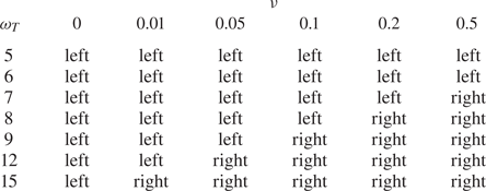
A version of figure 4 with enlarged panels broken into parts (a) through (d) for easier viewing. This version also includes collisionless ($\nu =0$ ) simulations. Time traces of the total radial heat flux ($Q$
 ) for Kinetic (blue), HP (orange), HPC (green), truncated (red), LMM-Middle (purple), LMM-Right (brown) and LMM-Left (pink) simulations for temperature gradient drives ($\omega _T$
 ) ranging from 5 to 15 (increasing downward by panel) and collision frequencies ($\nu$
 ) ranging from 0 to 0.5. The vertical blue lines show the cutoff point – 70 % of the simulation time – after which each heat flux curve is averaged to get the final saturation level.

Per cent error in saturated heat flux for each closure (HP, HPC, Truncation, LMM-Middle, LMM-Right, LMM-Left, LMM-Optimal (3 Point), LMM-Optimal (2 Point)) as compared against the kinetic simulation for temperature gradient drives ($\omega _T$ ) ranging from 5 to 15 (increasing downward) and collision frequency $\nu = 0$
 . Per cent errors are calculated as $(Q^{{\rm Closed}} - Q^{{\rm Kinetic}})/Q^{{\rm Kinetic}} \times 100$
 where $Q^{{\rm closed}}$
 is calculated by averaging the last 30 % of the time trace of the heat flux from the closed simulation and $Q^{{\rm Kinetic}}$
 is calculated by averaging the last 30 % of the time trace of the heat flux from the kinetic simulation. Average errors are calculated by averaging the absolute value of the errors.


 Open access