


1. Introduction
The modern information theory largely deals with information quantification, handling, compression, repossession and its storage. Numerous research studies have been carried out to avoid the information losses or error in these processes but at times they are unexpectedly involved. For instance, when there is insufficient information in the outcomes (e.g., lacking data) or the result contains erroneous information (e.g., due to model mis-specification), error or information loss is incurred. Kerridge [Reference Kerridge9] inaccuracy measure then plays a key role in understanding the resulted uncertainty and further describing reliability more accurately than the well-known uncertainty measure given by Shannon [Reference Shannon20]. Its primary significance lies in its ability to quantify the impact of inaccuracies in predicted probability distributions, providing a practical tool for analyzing model performance in real-world conditions. Unlike traditional measures like Kullback–Leibler (KL) divergence, which focus on the divergence between distributions, inaccuracy measure emphasizes on the practical consequences of using inaccurate models. This makes it highly relevant in fields such as economics, machine learning and risk assessment, where optimal decision strategies in the presence of uncertainty are pivotal.
Let the absolutely continuous and nonnegative random variables X and Y have probability density functions (pdfs) f and g associated with distribution functions (dfs) F and G, respectively. Then, the Kerridge inaccuracy measure between X and Y is given by
 \begin{equation}
\mathcal{I}_K(X,Y)=E_f[-\log{g(X)}]=-\int_{0}^{+\infty}f(x)\log{g(x)}dx.
\end{equation}
\begin{equation}
\mathcal{I}_K(X,Y)=E_f[-\log{g(X)}]=-\int_{0}^{+\infty}f(x)\log{g(x)}dx.
\end{equation} Precisely, it measures the expected difference when the outcomes of experiment suggest g as the pdf while f is the actual pdf. Note that “ $-\log{g(X)}$” with natural logarithm in (1.1) is interpreted as the information given by Y on suitability of X as a model. Eq. (1.1) provides a mathematical way to assess how well an estimated distribution captures the true underlying distribution and its lower value indicate that the estimated distribution is closer to the true distribution, while higher values indicate greater discrepancy. Some properties and applications of the above measure may be seen in Nair et al. [Reference Nair, Nair and Smitha16], Kumar et al. [Reference Kumar, Thapliyal and Taneja12], Smitha [Reference Smitha23], Parzen [Reference Parzen19], Kundu et al. [Reference Kundu, Di Crescenzo and Longobardi14] and Bueno and Balakrishnan [Reference Bueno and Balakrishnan4]. When $f\equiv g$ in the above equation, we get the classical measure of uncertainty known as Shannon’s entropy given by
 \begin{equation*}
\mathcal{H}(X)=-\int_{0}^{+\infty}f(x)\log{f(x)}dx.
\end{equation*}
\begin{equation*}
\mathcal{H}(X)=-\int_{0}^{+\infty}f(x)\log{f(x)}dx.
\end{equation*} In recent times, studying doubly truncated data has indeed become an important aspect across various fields, including survival studies, reliability theory, astronomy, forensic sciences and economics. The concept involves observing event times within specific intervals or with information limited to those intervals. Analyzing the doubly truncated data using mathematical and statistical tools is of particular interest, as are related to uncertainty measures. Let the random variable  $X_{t_1,t_2}=(X|t_1 \lt X \lt t_2)$ and similarly, $Y_{t_1,t_2}$ represent the lifetimes of systems failed in $(t_1,t_2)$, where t 1 and t 2 are such that
 \begin{equation}
(t_{1},t_{2})\in D=\{(u,v)\in \mathbb{R}_{+}^{2}:F(u) \lt F(v),G(u) \lt G(v)\}.
\end{equation}
\begin{equation}
(t_{1},t_{2})\in D=\{(u,v)\in \mathbb{R}_{+}^{2}:F(u) \lt F(v),G(u) \lt G(v)\}.
\end{equation} The df and pdf of the random variable  $X_{t_1,t_2}$ can thus be obtained as
 \begin{equation*}
F_{t_1,t_2}(x)=\frac{F(x)-F(t_1)}{F(t_2)-F(t_1)}~\text{and}~f_{t_1,t_2}(x)=\frac{f(x)}{F(t_2)-F(t_1)},
\end{equation*}
\begin{equation*}
F_{t_1,t_2}(x)=\frac{F(x)-F(t_1)}{F(t_2)-F(t_1)}~\text{and}~f_{t_1,t_2}(x)=\frac{f(x)}{F(t_2)-F(t_1)},
\end{equation*} respectively, and similar is the df and pdf for  $Y_{t_1,t_2}$. The interval inaccuracy measure for the random variables $X_{t_1,t_2}$ and $Y_{t_1,t_2}$ introduced by Kundu and Nanda [Reference Kundu and Nanda15] is given as
 \begin{align}
\mathcal{I}_K(X_{t_1,t_2},Y_{t_1,t_2})&= -\int_{t_1}^{t_2}f_{t_1,t_2}(x)\log{g_{t_1,t_2}(x)}dx\nonumber\\
&= -\int_{t_1}^{t_2}\frac{f(x)}{F(t_{2})-F(t_{1})}\log{\frac{g(x)}{G(t_{2})-G(t_{1})}}dx.
\end{align}
\begin{align}
\mathcal{I}_K(X_{t_1,t_2},Y_{t_1,t_2})&= -\int_{t_1}^{t_2}f_{t_1,t_2}(x)\log{g_{t_1,t_2}(x)}dx\nonumber\\
&= -\int_{t_1}^{t_2}\frac{f(x)}{F(t_{2})-F(t_{1})}\log{\frac{g(x)}{G(t_{2})-G(t_{1})}}dx.
\end{align} For a system survived to t 1 but observed to be down at t 2, (1.3) measures the overall uncertainty about its failure time between t 1 and t 2 extracted from the distribution of  $Y_{t_1,t_2}$ in place of the distribution of $X_{t_1,t_2}$.
As the usual measures of information are not self-sufficient to extract all the relevant information precisely, the focus has now been shifted toward the study of variance of information measures. Varinaccuracy, recently introduced by Balakrishnan et al. [Reference Balakrishnan, Buono, Cali and Longobardi2], is defined as the dispersion of information around the inaccuracy measure. Mathematically,
 \begin{align}
\mathcal{VI}_K(X,Y)&=\textrm{Var}_f[-\log{g(X)}]\nonumber\\
&=\int_{0}^{+\infty}f(x)(\log{g(x)})^2dx-[\mathcal{I}_K(X,Y)]^2.
\end{align}
\begin{align}
\mathcal{VI}_K(X,Y)&=\textrm{Var}_f[-\log{g(X)}]\nonumber\\
&=\int_{0}^{+\infty}f(x)(\log{g(x)})^2dx-[\mathcal{I}_K(X,Y)]^2.
\end{align} Intuitively, it describes the variability in the information given by  $g(\cdot)$ about the outcomes of $f(\cdot)$ and hence suggest how suitable the model is. The above measure is particularly useful when the inaccuracy measure is not adequate to compare and determine the appropriateness of preferred distributions. When $X\overset{d}=Y$, then (1.4) reduces to varentropy of the random variable X. Varentropy refers to the variance of the information content $-\log{f(\cdot)}$ around the differential entropy, which represents the expected information content of an absolutely continuous random variable. As a critical concept in information theory, varentropy measures the extent of dispersion of information content relative to entropy. Mathematically, varentropy of X (cf. [Reference Song24]) is defined as
 \begin{equation*}
\mathcal{V}(X)=\int_{0}^{+\infty}f(x)(\log{f(x)})^2dx-\left[\mathcal{H}(X)\right]^2.
\end{equation*}
\begin{equation*}
\mathcal{V}(X)=\int_{0}^{+\infty}f(x)(\log{f(x)})^2dx-\left[\mathcal{H}(X)\right]^2.
\end{equation*}One may find Bobkov and Madiman [Reference Bobkov and Madiman3], Arikan [Reference Arikan1], Fradelizi et al. [Reference Fradelizi, Madiman and Wang6] and Goodarzi et al. [Reference Goodarzi, Amini and Mohtashami Borzadaran7] to be useful for initial contributions on varentropy and further analyzing its relevance.
The second-order information measures have received increasing attention to study the variability of information. Note that varentropy is used to measure variability when assessing uncertainty is intrinsic to a single probability distribution. On the other hand, varinaccuracy extends this concept to a two-distribution framework and addresses the stochastic behavior of model misspecification by quantifying the variability around inaccuracy measure. This makes varinaccuracy especially suited for applications where accounting for both the first-order measure (inaccuracy) and its variability results in more informed model selection, improved assessment of model robustness and enhanced comparison of competing models under uncertainty. Similarly, dispersion based on KL divergence (cf. [Reference Balakrishnan, Buono, Cali and Longobardi2]) measures the variance of the log-likelihood ratio and captures the stability of the relative entropy between two distributions. However, in contexts where relative likelihood ratios are either undefined or lack interpretational clarity, varinaccuracy measure provides a more robust and interpretable alternative. Hence, varinaccuracy is a distinct and robust tool for analyzing second-order information behavior involving uncertainty about the underlying distribution.
Since the interval inaccuracy measure actively analyzes the reliability characteristics of system and its components from the information provided by the experimental observations falling in some time interval, analyzing the dispersion of this information is crucial. Moreover, the interval inaccuracy may not always identify the most appropriate model, yet analyzing the variability in information can offer additional insight. Furthermore, due to fixed values of t 1 and t 2, we anticipate better prediction of the system’s lifetime from the experimental observations when the data are doubly truncated. Thus, the study of interval varinaccuracy is significant and adds more reliance to the interval inaccuracy measure. Furthermore, this measure would help assess how sensitive the inaccuracy measure (1.1) is to changes in the truncation limits or underlying distributions, which is crucial for evaluating the robustness of statistical models. In fields such as reliability engineering, finance and astronomy, where doubly truncation frequently occurs, understanding the scatterness around the inaccuracy measure is expected to optimize estimation and prediction, refine model selection and support better decision-making. In particular, for reliability engineering, studying the varinaccuracy measure for doubly truncated random variables is particularly relevant when analyzing the lifespan of components tested within specific operational thresholds. For instance, if failure times are only recorded between a minimum detectable threshold and a maximum operational limit, understanding the dispersion around information inaccuracy helps ensure accurate reliability assessments, robust model selection and precise prediction of failure probabilities within the observed range. In finance, this analysis is expected to be valuable for modeling asset returns or risk metrics when data are constrained by lower and upper bounds, such as minimum investment thresholds and regulatory caps. It would ensure robust risk assessments and strengthen decision processes under restricted data conditions. The investigation of varinaccuracy for doubly truncated random variables is thus motivated, having applications in several domains related to reliability and life-testing.
The next section introduces a new varinaccuracy measure with reference to the interval life known as the interval (doubly truncated) varinaccuracy. Some examples have been presented following theoretical investigations and its several properties are studied. It is also investigated under certain class of common transformation and bounds have been obtained. In Section 3, we propose an estimator of the defined measure using smooth kernel-based nonparametric estimates followed by a simulation study analyzing the performance of the estimator in different intervals. The approach is further applied to two real data sets to substantiate the observations of the simulation study. Finally, an application of the proposed measure in the choice of parameter under proportional hazard rate model for the best alternative of any given distribution is presented in Section 4.
2. Interval varinaccuracy
The interval inaccuracy given by (1.3) is functional to measure the expected discrepancy between two probability distributions when restricted to some interval. To better analyze this uncertainty and have precision in the extracted information, the study of dispersion properties about this measure is motivated called as interval varinaccuracy. Additionally, the understanding of interval varinaccuracy would aid in gauging how errors in interval inaccuracy would affect the overall model performance. Moreover, it would assess the stability of the measure (1.3), crucial in determining robustness of the measure to uncertainties in data or modeling errors.
Let  $f_{t_1,t_2}(\cdot)$ and $g_{t_1,t_2}(\cdot)$ denote the pdfs of $X_{t_1,t_2}$ and $Y_{t_1,t_2}$, respectively, then the doubly truncated varinaccuracy measure for random variables X and Y is defined as
 \begin{align}
\mathcal{VI}_K(X_{t_1,t_2},Y_{t_1,t_2}) &= \textrm{Var}_{f_{t_1,t_2}}[-\log{g_{t_1,t_2}(X_{t_1,t_2})}] \nonumber\\
&= \int_{t_1}^{t_2}\frac{f(x)}{F(t_{2})-F(t_{1})}\left(\log{\frac{g(x)}{G(t_{2})-G(t_{1})}}\right)^2dx
-[\mathcal{I}_K(X_{t_1,t_2},Y_{t_1,t_2})]^2.
\end{align}
\begin{align}
\mathcal{VI}_K(X_{t_1,t_2},Y_{t_1,t_2}) &= \textrm{Var}_{f_{t_1,t_2}}[-\log{g_{t_1,t_2}(X_{t_1,t_2})}] \nonumber\\
&= \int_{t_1}^{t_2}\frac{f(x)}{F(t_{2})-F(t_{1})}\left(\log{\frac{g(x)}{G(t_{2})-G(t_{1})}}\right)^2dx
-[\mathcal{I}_K(X_{t_1,t_2},Y_{t_1,t_2})]^2.
\end{align} When  $X\overset{d}=Y$, then the above reduces to the interval varentropy for random variable X introduced by Sharma and Kundu [Reference Sharma and Kundu21] defined as
 \begin{equation*}
V(X_{t_1,t_2})=\int_{t_1}^{t_2}\frac{f(x)}{F(t_2)-F(t_1)}\left (\log{\frac{f(x)}{F(t_2)-F(t_1)}}\right )^2dx- [\mathcal{H}(X_{t_1,t_2})]^2,
\end{equation*}
\begin{equation*}
V(X_{t_1,t_2})=\int_{t_1}^{t_2}\frac{f(x)}{F(t_2)-F(t_1)}\left (\log{\frac{f(x)}{F(t_2)-F(t_1)}}\right )^2dx- [\mathcal{H}(X_{t_1,t_2})]^2,
\end{equation*} where  $\mathcal{H}(X_{t_1,t_2})$ is the doubly truncated entropy (cf. [Reference Sunoj, Sankaran and Maya25]) given by
 \begin{equation*}
\mathcal{H}(X_{t_1,t_2})=- \int_{t_1}^{t_2} \frac{f(x)}{F(t_2)-F(t_1)}\log{\frac{f(x)}{F(t_2)-F(t_1)}}dx.
\end{equation*}
\begin{equation*}
\mathcal{H}(X_{t_1,t_2})=- \int_{t_1}^{t_2} \frac{f(x)}{F(t_2)-F(t_1)}\log{\frac{f(x)}{F(t_2)-F(t_1)}}dx.
\end{equation*}On evaluating (2.5) further, we have
 \begin{equation}
\mathcal{VI}_K(X_{t_1,t_2},Y_{t_1,t_2})= \int_{t_1}^{t_2}\frac{f(x)}{F(t_{2})-F(t_{1})}\left(\log{g(x)}\right)^2dx
-[\Lambda_Y(t_1,t_2)+\mathcal{I}_K(X_{t_1,t_2},Y_{t_1,t_2})]^2;
\end{equation}
\begin{equation}
\mathcal{VI}_K(X_{t_1,t_2},Y_{t_1,t_2})= \int_{t_1}^{t_2}\frac{f(x)}{F(t_{2})-F(t_{1})}\left(\log{g(x)}\right)^2dx
-[\Lambda_Y(t_1,t_2)+\mathcal{I}_K(X_{t_1,t_2},Y_{t_1,t_2})]^2;
\end{equation} where  $\Lambda_Y(t_1,t_2)=-\log{(G(t_2)-G(t_1))}$. Note that (2.5) reduces to the measures known as residual varinaccuracy and past varinaccuracy studied by Sharma and Kundu [Reference Sharma and Kundu22] on substituting $t_{2}\rightarrow \infty$ and $t_{1}\rightarrow 0$, respectively. We asses the above definition by evaluating interval varinaccuracy for some cases considering significant distributions used in reliability and survival analysis.
Example 2.1. (i) Let the random lifetimes X and Y be distributed exponentially with parameters λ and η, respectively. Then, for  $(t_1,t_2)\in D$, (1.3) and (2.5) results in
 \begin{align*}
\mathcal{I}_K(X_{t_1,t_2},Y_{t_1,t_2}) &= \frac{\eta}{\lambda}+\log{\frac{e^{-\eta t_1}-e^{-\eta t_2}}{\eta}}+\eta \frac{t_1e^{-\lambda t_1}-t_2e^{-\lambda t_2}}{e^{-\lambda t_1}-e^{-\lambda t_2}}, \\
\mathcal{VI}_K(X_{t_1,t_2},Y_{t_1,t_2}) &= \left(\frac{\eta}{\lambda}\right)^2+\frac{\eta^2}{e^{-\lambda t_1}-e^{-\lambda t_2}}\left[\left(t_1^2e^{-\lambda t_1}-t_2^2e^{-\lambda t_2}\right)-\frac{(t_1e^{-\lambda t_1}-t_2e^{-\lambda t_2})^2}{e^{-\lambda t_1}-e^{-\lambda t_2}} \right].
\end{align*}
\begin{align*}
\mathcal{I}_K(X_{t_1,t_2},Y_{t_1,t_2}) &= \frac{\eta}{\lambda}+\log{\frac{e^{-\eta t_1}-e^{-\eta t_2}}{\eta}}+\eta \frac{t_1e^{-\lambda t_1}-t_2e^{-\lambda t_2}}{e^{-\lambda t_1}-e^{-\lambda t_2}}, \\
\mathcal{VI}_K(X_{t_1,t_2},Y_{t_1,t_2}) &= \left(\frac{\eta}{\lambda}\right)^2+\frac{\eta^2}{e^{-\lambda t_1}-e^{-\lambda t_2}}\left[\left(t_1^2e^{-\lambda t_1}-t_2^2e^{-\lambda t_2}\right)-\frac{(t_1e^{-\lambda t_1}-t_2e^{-\lambda t_2})^2}{e^{-\lambda t_1}-e^{-\lambda t_2}} \right].
\end{align*}Thus, the interval inaccuracy and varinaccuracy in this case is dependent on both time points t 1 and t 2. In case of exponential distribution where the exact parameter is different from the experimental parameter, the above formula may be used straightaway to obtain the expected inaccuracy and varinaccuracy for different time intervals.
(ii) Let X be uniformly distributed and Y having power distribution with parameter α in common support  $[0,1]$. Then, for $t_1,t_2\in[0,1]$ such that $(t_1,t_2)$ satisfies (1.2), the interval inaccuracy and varinaccuracy is evaluated as
 \begin{align*}
\mathcal{I}_K(X_{t_1,t_2},Y_{t_1,t_2}) &= \alpha-1-\log{\alpha}+\log{(t_2^\alpha-t_1^\alpha)}-(\alpha-1)\frac{t_2\log{t_2}-t_1\log{t_1}}{t_2-t_1},\\
\mathcal{VI}_K(X_{t_1,t_2},Y_{t_1,t_2}) &= (\alpha-1)^2 + \frac{(\alpha-1)^2}{t_2-t_1}\left[t_2(\log{t_2})^2-t_1(\log{t_1})^2-\frac{(t_2\log{t_2}-t_1\log{t_1})^2}{t_2-t_1}\right].
\end{align*}
\begin{align*}
\mathcal{I}_K(X_{t_1,t_2},Y_{t_1,t_2}) &= \alpha-1-\log{\alpha}+\log{(t_2^\alpha-t_1^\alpha)}-(\alpha-1)\frac{t_2\log{t_2}-t_1\log{t_1}}{t_2-t_1},\\
\mathcal{VI}_K(X_{t_1,t_2},Y_{t_1,t_2}) &= (\alpha-1)^2 + \frac{(\alpha-1)^2}{t_2-t_1}\left[t_2(\log{t_2})^2-t_1(\log{t_1})^2-\frac{(t_2\log{t_2}-t_1\log{t_1})^2}{t_2-t_1}\right].
\end{align*}It is clear that interval inaccuracy and varinaccuracy in this case is dependent on the time points t 1 and t 2 and the above formula may be used in practice where the interest is to evaluate the dispersion about the expected inaccuracy between uniform and power distributions for some given time interval.
A prominent relation among the inaccuracy, entropy and the KL [Reference Kullback10] divergence for  $X_{t_1,t_2}$ and $Y_{t_1,t_2}$, where $(t_1,t_2)\in D$ is given below
 \begin{equation}
\mathcal{I}_K(X_{t_1,t_2},Y_{t_1,t_2})=\mathcal{D}(X_{t_1,t_2},Y_{t_1,t_2})+\mathcal{H}(X_{t_1,t_2}),
\end{equation}
\begin{equation}
\mathcal{I}_K(X_{t_1,t_2},Y_{t_1,t_2})=\mathcal{D}(X_{t_1,t_2},Y_{t_1,t_2})+\mathcal{H}(X_{t_1,t_2}),
\end{equation}where
 \begin{equation}
\mathcal{D}(X_{t_1,t_2},Y_{t_1,t_2})=\int_{t_1}^{t_2}\frac{f(x)}{F(t_2)-F(t_1)}\log{\frac{f(x)/(F(t_2)-F(t_1))}
{g(x)/(G(t_2)-G(t_1))}}dx,
\end{equation}
\begin{equation}
\mathcal{D}(X_{t_1,t_2},Y_{t_1,t_2})=\int_{t_1}^{t_2}\frac{f(x)}{F(t_2)-F(t_1)}\log{\frac{f(x)/(F(t_2)-F(t_1))}
{g(x)/(G(t_2)-G(t_1))}}dx,
\end{equation}is the KL divergence for the given doubly truncated random variables. The above relation is useful to understand the additional uncertainty incurred because of the choice of a similar distribution in place of true distribution and quantifies the information in proportions. An analogous relation in terms of their dispersion indices would be functional to comprehend their scatterness of information aspect. The required correspondence is presented in the following theorem.
Theorem 2.1. Let  $X_{t_1,t_2}$ and $Y_{t_1,t_2}$ be two absolutely continuous and nonnegative random variables for $(t_1,t_2)$ given in (1.2). Then we have
 \begin{align*}
\mathcal{VI}_K(X_{t_1,t_2},Y_{t_1,t_2})&=\mathcal{VD}(X_{t_1,t_2},Y_{t_1,t_2})+\mathcal{V}(X_{t_1,t_2})\\
&\quad -2\textrm{Cov}_f\left(\log{\frac{f(x)/(F(t_2)-F(t_1))}
{g(x)/(G(t_2)-G(t_1))}},\log{\frac{f(x)}{F(t_2)-F(t_1)}}\bigg|t_1 \lt X \lt t_2 \right),
\end{align*}
\begin{align*}
\mathcal{VI}_K(X_{t_1,t_2},Y_{t_1,t_2})&=\mathcal{VD}(X_{t_1,t_2},Y_{t_1,t_2})+\mathcal{V}(X_{t_1,t_2})\\
&\quad -2\textrm{Cov}_f\left(\log{\frac{f(x)/(F(t_2)-F(t_1))}
{g(x)/(G(t_2)-G(t_1))}},\log{\frac{f(x)}{F(t_2)-F(t_1)}}\bigg|t_1 \lt X \lt t_2 \right),
\end{align*}where
 \begin{equation*}
\mathcal{VD}(X_{t_1,t_2},Y_{t_1,t_2})=\int_{t_1}^{t_2}\frac{f(x)}{F(t_2)-F(t_1)}\left(\log{\frac{f(x)/(F(t_2)-F(t_1))}
{g(x)/(G(t_2)-G(t_1))}}\right)^2dx-[\mathcal{D}(X_{t_1,t_2},Y_{t_1,t_2})]^2,
\end{equation*}
\begin{equation*}
\mathcal{VD}(X_{t_1,t_2},Y_{t_1,t_2})=\int_{t_1}^{t_2}\frac{f(x)}{F(t_2)-F(t_1)}\left(\log{\frac{f(x)/(F(t_2)-F(t_1))}
{g(x)/(G(t_2)-G(t_1))}}\right)^2dx-[\mathcal{D}(X_{t_1,t_2},Y_{t_1,t_2})]^2,
\end{equation*}is the dispersion index based on Eq. (2.8).
Proof. The first term of (2.5) may be written as
 \begin{eqnarray*}
&&\int_{t_1}^{t_2}\frac{f(x)}{F(t_{2})-F(t_{1})}\left(\log{\frac{g(x)}{G(t_{2})-G(t_{1})}}\right)^2dx\\
&&= \int_{t_1}^{t_2}\frac{f(x)}{F(t_{2})-F(t_{1})}
\left(\log{\left(\frac{f(x)}{F(t_2)-F(t_1)}\cdot\frac{g(x)/(G(t_2)-G(t_1))}{f(x)/(F(t_2)-F(t_1))}\right)}\right)^2dx.
\end{eqnarray*}
\begin{eqnarray*}
&&\int_{t_1}^{t_2}\frac{f(x)}{F(t_{2})-F(t_{1})}\left(\log{\frac{g(x)}{G(t_{2})-G(t_{1})}}\right)^2dx\\
&&= \int_{t_1}^{t_2}\frac{f(x)}{F(t_{2})-F(t_{1})}
\left(\log{\left(\frac{f(x)}{F(t_2)-F(t_1)}\cdot\frac{g(x)/(G(t_2)-G(t_1))}{f(x)/(F(t_2)-F(t_1))}\right)}\right)^2dx.
\end{eqnarray*}On further expanding the squares, note that
 \begin{eqnarray*}
&&-2\int_{t_1}^{t_2}\frac{f(x)}{F(t_2)-F(t_1)}\log{\frac{f(x)}{F(t_2)-F(t_1)}}\cdot \log{\frac{f(x)/(F(t_2)-F(t_1))}
{g(x)/(G(t_2)-G(t_1))}} dx\\
&&+2\int_{t_1}^{t_2}\frac{f(x)}{F(t_2)-F(t_1)}\log{\frac{f(x)}{F(t_2)-F(t_1)}}dx\cdot \int_{t_1}^{t_2}\frac{f(x)}{F(t_2)-F(t_1)}\log{\frac{f(x)/(F(t_2)-F(t_1))}
{g(x)/(G(t_2)-G(t_1))}} dx\\
&&=-2\textrm{Cov}_f\left(\log{\frac{f(x)/(F(t_2)-F(t_1))}
{g(x)/(G(t_2)-G(t_1))}},\log{\frac{f(x)}{F(t_2)-F(t_1)}}\bigg|t_1 \lt X \lt t_2 \right).
\end{eqnarray*}
\begin{eqnarray*}
&&-2\int_{t_1}^{t_2}\frac{f(x)}{F(t_2)-F(t_1)}\log{\frac{f(x)}{F(t_2)-F(t_1)}}\cdot \log{\frac{f(x)/(F(t_2)-F(t_1))}
{g(x)/(G(t_2)-G(t_1))}} dx\\
&&+2\int_{t_1}^{t_2}\frac{f(x)}{F(t_2)-F(t_1)}\log{\frac{f(x)}{F(t_2)-F(t_1)}}dx\cdot \int_{t_1}^{t_2}\frac{f(x)}{F(t_2)-F(t_1)}\log{\frac{f(x)/(F(t_2)-F(t_1))}
{g(x)/(G(t_2)-G(t_1))}} dx\\
&&=-2\textrm{Cov}_f\left(\log{\frac{f(x)/(F(t_2)-F(t_1))}
{g(x)/(G(t_2)-G(t_1))}},\log{\frac{f(x)}{F(t_2)-F(t_1)}}\bigg|t_1 \lt X \lt t_2 \right).
\end{eqnarray*}Making use of the above and (2.7) in the expression of interval varinaccuracy given in Eq. (2.5), we obtain the stated relation.
2.1. Properties
In this part, we study some useful properties of the measure given in (2.5) based on monotonicty and relationship under transformations.
2.1.1. Monotonicity properties
The following counterexample is given to conclude that the interval varinaccuracy measure may be nonincreasing with respect to both t 1 and t 2, respectively, on keeping the other fixed.
Counter Example 2.1. Suppose  $X\sim U(0,2)$ and Y has df
 \begin{equation*}
G(x) = \left\{\begin{array}{ll} \exp\left( -\frac{1}{2}-\frac{1}{x}\right),
\,\,\,\,\,\, ~for~ 0 \leq x \leq 1\\
\exp\left( -2+\frac{x^2}{2}\right),
\,\,\,\,\, ~for~ 1 \leq x \leq 2.\end{array}\right.
\end{equation*}
\begin{equation*}
G(x) = \left\{\begin{array}{ll} \exp\left( -\frac{1}{2}-\frac{1}{x}\right),
\,\,\,\,\,\, ~for~ 0 \leq x \leq 1\\
\exp\left( -2+\frac{x^2}{2}\right),
\,\,\,\,\, ~for~ 1 \leq x \leq 2.\end{array}\right.
\end{equation*}Then, Figure 1 shows that doubly truncated varinaccuracy for this pair of distributions is not monotone in t 1 and t 2, respectively, for fixed value of the other. The above example demonstrates that the nature of interval varinaccuracy is influenced not only by the specific time points but also by the chosen probability distributions.
Furthermore, we present compact expressions to evaluate the change in the doubly truncated varinaccuracy with respect to the truncation points t 1 and t 2, respectively. This may be useful to investigate other properties of interest such as its constancy, relation with varinaccuracy measure and others. Before that, we recall the generalized failure rate (GFR) functions of a doubly truncated random variable  $(X|t_1 \lt X \lt t_2)$ (cf. [Reference Navarro and Ruiz17]) are given as
 \begin{equation*}
h_1^X(t_1,t_2)=\frac{f(t_1)}{F(t_2)-F(t_1)}~~\text{and}~~h_2^X(t_1,t_2)=\frac{f(t_2)}{F(t_2)-F(t_1)}.
\end{equation*}
\begin{equation*}
h_1^X(t_1,t_2)=\frac{f(t_1)}{F(t_2)-F(t_1)}~~\text{and}~~h_2^X(t_1,t_2)=\frac{f(t_2)}{F(t_2)-F(t_1)}.
\end{equation*} Similarly,  $h_1^Y(t_1,t_2)$ and $h_2^Y(t_1,t_2)$ may be defined for the random variable $(Y|t_1 \lt Y \lt t_2)$. Also, note that (cf. [Reference Kundu and Nanda15])
 \begin{align}
\frac{\partial \mathcal{I}_K(X_{t_1,t_2},Y_{t_1,t_2})}{\partial t_{1}} &= h_1^X(t_1,t_2)\left [\mathcal{I}_K(X_{t_1,t_2},Y_{t_1,t_2})+ \log{h_1^Y(t_1,t_2)} \right]-h_1^Y(t_1,t_2),
\end{align}
\begin{align}
\frac{\partial \mathcal{I}_K(X_{t_1,t_2},Y_{t_1,t_2})}{\partial t_{1}} &= h_1^X(t_1,t_2)\left [\mathcal{I}_K(X_{t_1,t_2},Y_{t_1,t_2})+ \log{h_1^Y(t_1,t_2)} \right]-h_1^Y(t_1,t_2),
\end{align} \begin{align}
\frac{\partial \mathcal{I}_K(X_{t_1,t_2},Y_{t_1,t_2})}{\partial t_{2}} &= -h_2^X(t_1,t_2)\left [\mathcal{I}_K(X_{t_1,t_2},Y_{t_1,t_2})+ \log{h_2^Y(t_1,t_2)} \right]+h_2^Y(t_1,t_2).
\end{align}
\begin{align}
\frac{\partial \mathcal{I}_K(X_{t_1,t_2},Y_{t_1,t_2})}{\partial t_{2}} &= -h_2^X(t_1,t_2)\left [\mathcal{I}_K(X_{t_1,t_2},Y_{t_1,t_2})+ \log{h_2^Y(t_1,t_2)} \right]+h_2^Y(t_1,t_2).
\end{align}Proposition 2.1. For the random variables  $X_{t_1,t_2}$ and $Y_{t_1,t_2}$ such that $(t_1,t_2)\in D$, the derivatives of the doubly truncated varinaccuracy are
 \begin{align*}
\frac{\partial \mathcal{VI}_K(X_{t_1,t_2},Y_{t_1,t_2})}{\partial t_1} = h_1^X(t_1,t_2)\left [ \mathcal{VI}_K(X_{t_1,t_2},Y_{t_1,t_2})- \left (\mathcal{I}_K(X_{t_1,t_2},Y_{t_1,t_2}) + \log h_1^Y(t_1,t_2)\right )^2\right]; \\
\frac{\partial \mathcal{VI}_K(X_{t_1,t_2},Y_{t_1,t_2})}{\partial t_2} = -h_2^X(t_1,t_2)\left [ \mathcal{VI}_K(X_{t_1,t_2},Y_{t_1,t_2})- \left (\mathcal{I}_K(X_{t_1,t_2},Y_{t_1,t_2}) + \log h_2^Y(t_1,t_2)\right )^2\right].
\end{align*}
\begin{align*}
\frac{\partial \mathcal{VI}_K(X_{t_1,t_2},Y_{t_1,t_2})}{\partial t_1} = h_1^X(t_1,t_2)\left [ \mathcal{VI}_K(X_{t_1,t_2},Y_{t_1,t_2})- \left (\mathcal{I}_K(X_{t_1,t_2},Y_{t_1,t_2}) + \log h_1^Y(t_1,t_2)\right )^2\right]; \\
\frac{\partial \mathcal{VI}_K(X_{t_1,t_2},Y_{t_1,t_2})}{\partial t_2} = -h_2^X(t_1,t_2)\left [ \mathcal{VI}_K(X_{t_1,t_2},Y_{t_1,t_2})- \left (\mathcal{I}_K(X_{t_1,t_2},Y_{t_1,t_2}) + \log h_2^Y(t_1,t_2)\right )^2\right].
\end{align*}Graph of interval varinaccuracy with respect to t 1 and t 2, respectively, on keeping the other fixed (Counterexample 2.1).

Proof. On differentiating (2.6), we obtain
 \begin{align*}
\frac{\partial \mathcal{VI}_K(X_{t_1,t_2},Y_{t_1,t_2})}{\partial t_{1}} &= \frac{h_1^X(t_1,t_2)}{F(t_2)-F(t_1)}\int_{t_1}^{t_2}f(x)(\log g(x))^2dx - h_1^X(t_1,t_2)(\log g(t_1))^2 \\
&\quad -2\big( \Lambda_Y(t_1,t_2) + \mathcal{I}_K(X_{t_1,t_2},Y_{t_1,t_2})\big)\left ( h_1^Y(t_1,t_2) + \frac{\partial \mathcal{I}_K(X_{t_1,t_2},Y_{t_1,t_2})}{\partial t_{1}}\right ),\\
\frac{\partial \mathcal{VI}_K(X_{t_1,t_2},Y_{t_1,t_2})}{\partial t_2} &= \frac{- h_2^X(t_1,t_2)}{F(t_2)-F(t_1)}\int_{t_1}^{t_2}f(x)(\log g(x))^2dx + h_2^X(t_1,t_2)(\log g(t_2))^2 \\
&\quad -2\big( \Lambda_Y(t_1,t_2) + \mathcal{I}_K(X_{t_1,t_2},Y_{t_1,t_2})\big)\left ( -h_2^Y(t_1,t_2) + \frac{\partial \mathcal{I}_K(X_{t_1,t_2},Y_{t_1,t_2})}{\partial t_{2}}\right ).
\end{align*}
\begin{align*}
\frac{\partial \mathcal{VI}_K(X_{t_1,t_2},Y_{t_1,t_2})}{\partial t_{1}} &= \frac{h_1^X(t_1,t_2)}{F(t_2)-F(t_1)}\int_{t_1}^{t_2}f(x)(\log g(x))^2dx - h_1^X(t_1,t_2)(\log g(t_1))^2 \\
&\quad -2\big( \Lambda_Y(t_1,t_2) + \mathcal{I}_K(X_{t_1,t_2},Y_{t_1,t_2})\big)\left ( h_1^Y(t_1,t_2) + \frac{\partial \mathcal{I}_K(X_{t_1,t_2},Y_{t_1,t_2})}{\partial t_{1}}\right ),\\
\frac{\partial \mathcal{VI}_K(X_{t_1,t_2},Y_{t_1,t_2})}{\partial t_2} &= \frac{- h_2^X(t_1,t_2)}{F(t_2)-F(t_1)}\int_{t_1}^{t_2}f(x)(\log g(x))^2dx + h_2^X(t_1,t_2)(\log g(t_2))^2 \\
&\quad -2\big( \Lambda_Y(t_1,t_2) + \mathcal{I}_K(X_{t_1,t_2},Y_{t_1,t_2})\big)\left ( -h_2^Y(t_1,t_2) + \frac{\partial \mathcal{I}_K(X_{t_1,t_2},Y_{t_1,t_2})}{\partial t_{2}}\right ).
\end{align*} The values of  $\dfrac{\partial \mathcal{I}_K(X_{t_1,t_2}Y_{t_1,t_2})}{\partial t_{1}}$ and $\dfrac{\partial \mathcal{I}_K(X_{t_1,t_2},Y_{t_1,t_2})}{\partial t_{2}}$ from (2.9) and (2.10), respectively, when substituted yield
 \begin{align*}
\frac{\partial \mathcal{VI}_K(X_{t_1,t_2},Y_{t_1,t_2})}{\partial t_{1}} &= h_1^X(t_1,t_2) [ \mathcal{VI}_K(X_{t_1,t_2},Y_{t_1,t_2})+ \left ( \Lambda_Y(t_1,t_2)+ \mathcal{I}_K(X_{t_1,t_2},Y_{t_1,t_2})\right )^2\\
&\quad -(\log{g(t_1)})^{2}
-2\left( \Lambda_Y(t_1,t_2)+ \mathcal{I}_K(X_{t_1,t_2},Y_{t_1,t_2})\right)\\
&\quad \times(\log{h_1^Y(t_1,t_2)} + \mathcal{I}_K(X_{t_1,t_2},Y_{t_1,t_2}) ) ],
\end{align*}
\begin{align*}
\frac{\partial \mathcal{VI}_K(X_{t_1,t_2},Y_{t_1,t_2})}{\partial t_{1}} &= h_1^X(t_1,t_2) [ \mathcal{VI}_K(X_{t_1,t_2},Y_{t_1,t_2})+ \left ( \Lambda_Y(t_1,t_2)+ \mathcal{I}_K(X_{t_1,t_2},Y_{t_1,t_2})\right )^2\\
&\quad -(\log{g(t_1)})^{2}
-2\left( \Lambda_Y(t_1,t_2)+ \mathcal{I}_K(X_{t_1,t_2},Y_{t_1,t_2})\right)\\
&\quad \times(\log{h_1^Y(t_1,t_2)} + \mathcal{I}_K(X_{t_1,t_2},Y_{t_1,t_2}) ) ],
\end{align*} \begin{align*}
\frac{\partial \mathcal{VI}_K(X_{t_1,t_2},Y_{t_1,t_2})}{\partial t_2} &= -h_2^X(t_1,t_2) [ \mathcal{VI}_K(X_{t_1,t_2},Y_{t_1,t_2})+ \left ( \Lambda_Y(t_1,t_2)+ \mathcal{I}_K(X_{t_1,t_2},Y_{t_1,t_2})\right )^2\\
&\quad -(\log{g(t_2)})^{2}
-2( \Lambda_Y(t_1,t_2)+ \mathcal{I}_K(X_{t_1,t_2},Y_{t_1,t_2}))\\
&\quad \times(\log{h_2^Y(t_1,t_2)} + \mathcal{I}_K(X_{t_1,t_2},Y_{t_1,t_2})) ].
\end{align*}
\begin{align*}
\frac{\partial \mathcal{VI}_K(X_{t_1,t_2},Y_{t_1,t_2})}{\partial t_2} &= -h_2^X(t_1,t_2) [ \mathcal{VI}_K(X_{t_1,t_2},Y_{t_1,t_2})+ \left ( \Lambda_Y(t_1,t_2)+ \mathcal{I}_K(X_{t_1,t_2},Y_{t_1,t_2})\right )^2\\
&\quad -(\log{g(t_2)})^{2}
-2( \Lambda_Y(t_1,t_2)+ \mathcal{I}_K(X_{t_1,t_2},Y_{t_1,t_2}))\\
&\quad \times(\log{h_2^Y(t_1,t_2)} + \mathcal{I}_K(X_{t_1,t_2},Y_{t_1,t_2})) ].
\end{align*}Following some arrangements, the required result is achieved.
The above proposition may be used to evaluate the rate of change of varinaccuracy between two given distributions at any specific time point t 1 and t 2 when the other is fixed providing understanding of the system’s behavior to optimize it effectively and for other decision-making. A characterization of uniform distribution in terms of interval varinaccuracy is given below.
Proposition 2.2. Let the random variables X and Y have same support (a, b). Then  $\mathcal{VI}_K(X_{t_1,t_2},Y_{t_1,t_2})=0$, for all $(t_1,t_2)\in D$ if and only if Y is uniformly distributed on (a, b).
Proof. The concept of interval varinaccuracy given in (2.5) is defined as a variance measure that becomes zero only for degenerate distributions. Specifically, for  $x\in(a,b)$ such that $(t_1,t_2)\in D$, $\log{\frac{g(x)}{G(t_2)-G(t_1)}}$ must remain constant, implying $g(\cdot)$ must be a constant function and Y follows a uniform distribution over (a, b).
This property can be used in practice to test for uniformity, optimize systems requiring evenly distributed probabilities or analyze the inaccuracy and varinaccuracy in information theory applications where uniformity is of interest in time intervals. To derive the conditions resulting to constant interval varinaccuracy, we have the following theorem.
Theorem 2.2. (i) Let us assume the doubly truncated varinaccuracy  $\mathcal{VI}_K(X_{t_1,t_2},Y_{t_1,t_2})$ to be constant, that is, $\mathcal{VI}_K(X_{t_1,t_2},Y_{t_1,t_2})=v\geq0$ for all $(t_1,t_2)\in D$. Then
 \begin{eqnarray*}
|\mathcal{I}_K(X_{t_1,t_2},Y_{t_1,t_2}) + \log{h_1^Y(t_1,t_2)} | &=& \sqrt{v} \\
{\rm and}~~~|\mathcal{I}_K(X_{t_1,t_2},Y_{t_1,t_2}) + \log{h_2^Y(t_1,t_2)}| &=& \sqrt{v}, \forall \,\,(t_1,t_2) \in D.
\end{eqnarray*}
\begin{eqnarray*}
|\mathcal{I}_K(X_{t_1,t_2},Y_{t_1,t_2}) + \log{h_1^Y(t_1,t_2)} | &=& \sqrt{v} \\
{\rm and}~~~|\mathcal{I}_K(X_{t_1,t_2},Y_{t_1,t_2}) + \log{h_2^Y(t_1,t_2)}| &=& \sqrt{v}, \forall \,\,(t_1,t_2) \in D.
\end{eqnarray*} (ii) Suppose that  $\forall (t_1,t_2) \in D$ and $c\in\mathbb{R}$, any one of the following conditions holds
 \begin{align} \mathcal{I}_K(X_{t_1,t_2},Y_{t_1,t_2}) + \log{h_1^Y(t_1,t_2)} = c,
\end{align}
\begin{align} \mathcal{I}_K(X_{t_1,t_2},Y_{t_1,t_2}) + \log{h_1^Y(t_1,t_2)} = c,
\end{align} \begin{align} \mathcal{I}_K(X_{t_1,t_2},Y_{t_1,t_2}) + \log{h_2^Y(t_1,t_2)} = c
\end{align}
\begin{align} \mathcal{I}_K(X_{t_1,t_2},Y_{t_1,t_2}) + \log{h_2^Y(t_1,t_2)} = c
\end{align}then
 \begin{equation}
\lvert \mathcal{VI}_K(X_{t_1,t_2},Y_{t_1,t_2})- c^{2}\rvert = \frac{|\mathcal{VI}_K(X,Y)-c^{2}|}{F(t_{2})-F(t_{1})}.
\end{equation}
\begin{equation}
\lvert \mathcal{VI}_K(X_{t_1,t_2},Y_{t_1,t_2})- c^{2}\rvert = \frac{|\mathcal{VI}_K(X,Y)-c^{2}|}{F(t_{2})-F(t_{1})}.
\end{equation}Proof. (i) The proof is straightforward following Proposition 2.1, on assuming interval varinaccuracy to be constant v.
(ii) Proposition 2.1 with the assumption (2.11) gives
 \begin{equation*}
\frac{\partial \mathcal{VI}_K(X_{t_1,t_2},Y_{t_1,t_2})}{\partial t_{1}} = h_1^X(t_1,t_2)\left [ \mathcal{VI}_K(X_{t_1,t_2},Y_{t_1,t_2})- c^2\right].
\end{equation*}
\begin{equation*}
\frac{\partial \mathcal{VI}_K(X_{t_1,t_2},Y_{t_1,t_2})}{\partial t_{1}} = h_1^X(t_1,t_2)\left [ \mathcal{VI}_K(X_{t_1,t_2},Y_{t_1,t_2})- c^2\right].
\end{equation*}The above partial differential equation is solved to obtain
 \begin{equation*}
\log{\lvert \mathcal{VI}_K(X_{t_1,t_2},Y_{t_1,t_2})-c^2\rvert}=\log{\frac{c_1}{F(t_2)-F(t_1)}}.
\end{equation*}
\begin{equation*}
\log{\lvert \mathcal{VI}_K(X_{t_1,t_2},Y_{t_1,t_2})-c^2\rvert}=\log{\frac{c_1}{F(t_2)-F(t_1)}}.
\end{equation*}On using the boundary condition
 \begin{equation*}
\lim_{t_{1}\to \underset{D}\inf ~u, t_{2}\to \underset{D}\sup ~v} \mathcal{VI}_K(X_{t_1,t_2},Y_{t_1,t_2})=\mathcal{VI}_K(X,Y),
\end{equation*}
\begin{equation*}
\lim_{t_{1}\to \underset{D}\inf ~u, t_{2}\to \underset{D}\sup ~v} \mathcal{VI}_K(X_{t_1,t_2},Y_{t_1,t_2})=\mathcal{VI}_K(X,Y),
\end{equation*} where  $\underset{D}\inf ~u = a$ and $\underset{D}\sup ~v = b$, say such that $F(a)=0$ and $F(b)=1$, the integration constant c 1 is
 \begin{equation*}
\log{\lvert \mathcal{VI}_K(X,Y)-c^2\rvert}=\log{c_1},
\end{equation*}
\begin{equation*}
\log{\lvert \mathcal{VI}_K(X,Y)-c^2\rvert}=\log{c_1},
\end{equation*}or equivalently,
 \begin{equation*}
c_1=\lvert \mathcal{VI}_K(X,Y)-c^2\rvert.
\end{equation*}
\begin{equation*}
c_1=\lvert \mathcal{VI}_K(X,Y)-c^2\rvert.
\end{equation*}Thus, Eq. (2.13) is attained on substituting the value of c 1 in the solution. The same result is obtained if we proceed as above with (2.12).
The above theorem may be used to obtain interval varinaccuracy between two distributions effortlessly under the given condition. The example below is an application of the above theorem.
Example 2.2. Let X and Y have same support (a, b) and let Y be uniformly distributed therein. Then,  $\mathcal{VI}_K(X_{t_1,t_2},Y_{t_1,t_2})$ is constant $\left(=0\right)$, for all $(t_1,t_2)\in D$ on following Proposition 2.2. We apply Theorem 2.2(i) and obtain
 \begin{eqnarray*}
\mathcal{I}_K(X_{t_1,t_2},Y_{t_1,t_2}) + \log{h_1^Y(t_1,t_2)} &=& 0, \\
{\rm and}~~~\mathcal{I}_K(X_{t_1,t_2},Y_{t_1,t_2}) + \log{h_2^Y(t_1,t_2)} &=& 0.
\end{eqnarray*}
\begin{eqnarray*}
\mathcal{I}_K(X_{t_1,t_2},Y_{t_1,t_2}) + \log{h_1^Y(t_1,t_2)} &=& 0, \\
{\rm and}~~~\mathcal{I}_K(X_{t_1,t_2},Y_{t_1,t_2}) + \log{h_2^Y(t_1,t_2)} &=& 0.
\end{eqnarray*} On the other hand, assuming the above expressions to hold for all  $(t_1,t_2)\in D$ and applying Theorem 2.2(ii), we observe that the right hand side (RHS) of the given relation vanishes $\left(\because\mathcal{VI}_K(X,Y)=0\right)$ and so the interval varinaccuracy is 0.
Remark 2.1. If (2.11) and (2.12) hold simultaneously in theorem 2.2 then  $h_1^Y(t_1,t_2)=h_2^Y(t_1,t_2)$ which implies $g(t_1)=g(t_2),~\forall (t_1,t_2) \in D$. Hence, Y must be a uniformly distributed random variable for which its corresponding interval varinaccuracy is constant. That is, the converse of Theorem 2.2(i) holds and results in the characterization of random variable Y as uniform distribution in the respective domain.
The parametric form of the GFR function helps model varied failure patterns and improve reliability predictions. Recall the parametric form of GFR functions proposed by Sharma and Kundu [Reference Sharma and Kundu21] for  $c\in\mathbb{R}$ as
 \begin{equation*}
h_{1,c}^X(t_1,t_2)=\frac{f(t_1)}{[F(t_2)-F(t_1)]^{1-c}}~~\text{and}~~
h_{2,c}^X(t_1,t_2)=\frac{f(t_2)}{[F(t_2)-F(t_1)]^{1-c}},
\end{equation*}
\begin{equation*}
h_{1,c}^X(t_1,t_2)=\frac{f(t_1)}{[F(t_2)-F(t_1)]^{1-c}}~~\text{and}~~
h_{2,c}^X(t_1,t_2)=\frac{f(t_2)}{[F(t_2)-F(t_1)]^{1-c}},
\end{equation*} and the concept of generalized proportional hazard rate (GPHR) model given by Kundu [Reference Kundu13] for  $0 \lt \theta\in\mathbb{R}$ as
 \begin{equation*}
h_i^Y(t_1,t_2)=\theta h_i^X(t_1,t_2),~~~i=1,2;
\end{equation*}
\begin{equation*}
h_i^Y(t_1,t_2)=\theta h_i^X(t_1,t_2),~~~i=1,2;
\end{equation*} for  $(t_1,t_2)\in D$. The GPHR is vital for connecting failure rates, assuming that the fundamental failure rate function of the true distribution is similar to that of the choice of reference distribution, leading to improved predictions and more consistent analysis of survival or failure behavior. The next theorem aims to generalize the conditions of Theorem 2.2 under GPHR where the constancy of the parametric GFR functions may simplify the modeling by assuming a stable risk over time, enabling reliable predictions and consistent comparisons of survival or failure behaviors.
Theorem 2.3. Let  $(X|t_1 \lt X \lt t_2)$ and $(Y|t_1 \lt Y \lt t_2)$ be the doubly truncated random variables where $(t_1,t_2)$ satisfies (1.2). The parametric GFR functions of X having parameter $\theta-c$ are constant, that is,
 \begin{equation*}
\theta h_{1,\theta-c}^X(t_1,t_2)=e^{c-\mathcal{I}_K(X,Y)}~~\text{and}~~\theta h_{2,\theta-c}^X(t_1,t_2)=e^{c-\mathcal{I}_K(X,Y)}, \forall \,\,(t_{1},t_{2}) \in D,
\end{equation*}
\begin{equation*}
\theta h_{1,\theta-c}^X(t_1,t_2)=e^{c-\mathcal{I}_K(X,Y)}~~\text{and}~~\theta h_{2,\theta-c}^X(t_1,t_2)=e^{c-\mathcal{I}_K(X,Y)}, \forall \,\,(t_{1},t_{2}) \in D,
\end{equation*}Proof. Let us assume (2.11) hold. Then
 \begin{eqnarray*}
\frac{\partial \mathcal{I}_K(X_{t_1,t_2},Y_{t_1,t_2})}{\partial t_{1}} &=& h_1^X(t_1,t_2)[c-\theta].
\end{eqnarray*}
\begin{eqnarray*}
\frac{\partial \mathcal{I}_K(X_{t_1,t_2},Y_{t_1,t_2})}{\partial t_{1}} &=& h_1^X(t_1,t_2)[c-\theta].
\end{eqnarray*}On partially integrating the above equation, we obtain
 \begin{eqnarray*}
\mathcal{I}_K(X_{t_1,t_2},Y_{t_1,t_2})&=& \mathcal{I}_K(X,Y)-\log{(F(t_{2})-F(t_{1}))^{c-\theta}},
\end{eqnarray*}
\begin{eqnarray*}
\mathcal{I}_K(X_{t_1,t_2},Y_{t_1,t_2})&=& \mathcal{I}_K(X,Y)-\log{(F(t_{2})-F(t_{1}))^{c-\theta}},
\end{eqnarray*}which on using (2.11) again yields
 \begin{eqnarray*}
c-\log{\theta}= \mathcal{I}_K(X,Y) + \log{\frac{f(t_1)}{(F(t_2)-F(t_1))^{1-\theta+c}}}.
\end{eqnarray*}
\begin{eqnarray*}
c-\log{\theta}= \mathcal{I}_K(X,Y) + \log{\frac{f(t_1)}{(F(t_2)-F(t_1))^{1-\theta+c}}}.
\end{eqnarray*}Thus, we get the required expression. On proceeding as above with (2.12), the other part is obtained.
2.1.2. Relationship under transformations
The expression of interval varinaccuracy in compact form through conventional method might be challenging for some distributions. Transformations can sometimes simplify the evaluation of interval varinaccuracy for certain distributions, particularly when the interval varinaccuracy of the parent distribution is already known. The study of transformations, therefore, serves as a crucial tool to compute the interval varinaccuracy more efficiently and analyze all inherited relationships. We begin by examining the doubly truncated varinaccuracy for affine transformations, followed by its extension to a more general class of transformations, specifically those that are differentiable and strictly monotone. Recall that
 \begin{equation*}
\tilde{X}=aX+b ~\text{and}~\tilde{Y}=aY+b,~~~a \gt 0,b\geq 0;
\end{equation*}
\begin{equation*}
\tilde{X}=aX+b ~\text{and}~\tilde{Y}=aY+b,~~~a \gt 0,b\geq 0;
\end{equation*} the inaccuracy between the transformed random variables in interval  $(t_1,t_2)$ is given by
 \begin{equation}
\mathcal{I}_K(\tilde{X}_{t_1,t_2},\tilde{Y}_{t_1,t_2})=
\mathcal{I}_K\left(X_{\frac{t_1-b}{a},\frac{t_2-b}{a}},Y_{\frac{t_1-b}{a},\frac{t_2-b}{a}}\right)+\log{a}.
\end{equation}
\begin{equation}
\mathcal{I}_K(\tilde{X}_{t_1,t_2},\tilde{Y}_{t_1,t_2})=
\mathcal{I}_K\left(X_{\frac{t_1-b}{a},\frac{t_2-b}{a}},Y_{\frac{t_1-b}{a},\frac{t_2-b}{a}}\right)+\log{a}.
\end{equation}The relation for their doubly truncated varinaccuracy is given below.
Proposition 2.3. Let the random variables  $\tilde{X}$ and $\tilde{Y}$ be the respective affine transformations of X and Y. Then for all $(t_1,t_2)\in D$, we have
 \begin{equation*}
\mathcal{VI}_K(\tilde{X}_{t_1,t_2},\tilde{Y}_{t_1,t_2})=
\mathcal{VI}_K\left(X_{\frac{t_1-b}{a},\frac{t_2-b}{a}},Y_{\frac{t_1-b}{a},\frac{t_2-b}{a}}\right), 0 \leq b \lt t_{1} \lt t_{2}.
\end{equation*}
\begin{equation*}
\mathcal{VI}_K(\tilde{X}_{t_1,t_2},\tilde{Y}_{t_1,t_2})=
\mathcal{VI}_K\left(X_{\frac{t_1-b}{a},\frac{t_2-b}{a}},Y_{\frac{t_1-b}{a},\frac{t_2-b}{a}}\right), 0 \leq b \lt t_{1} \lt t_{2}.
\end{equation*}Proof. Let  $\tilde{X}$ and $\tilde{Y}$ have dfs $\tilde{F}(\cdot)$ and $\tilde{G}(\cdot)$, respectively. Then
 \begin{equation*}
\tilde{F}(t)=F\left(\frac{t-b}{a}\right)~~\text{and}~~ \tilde{G}(t)=G\left(\frac{t-b}{a}\right),~~~\forall t\geq b.
\end{equation*}
\begin{equation*}
\tilde{F}(t)=F\left(\frac{t-b}{a}\right)~~\text{and}~~ \tilde{G}(t)=G\left(\frac{t-b}{a}\right),~~~\forall t\geq b.
\end{equation*}Substituting (2.14) in the expression of doubly truncated varinaccuracy gives
 \begin{align*}
\mathcal{VI}_K(\tilde{X}_{t_1,t_2},\tilde{Y}_{t_1,t_2})&=
\int_{\frac{t_1-b}{a}}^{\frac{t_2-b}{a}}\frac{f(x)}{F(\frac{t_2-b}{a})-F(\frac{t_1-b}{a})}
\left(\log{\frac{g(x)}{G(\frac{t_2-b}{a})-G(\frac{t_1-b}{a})}}-\log{a}\right)^2dx\\
&\quad -\left[\mathcal{I}_K\left(X_{\frac{t_1-b}{a},\frac{t_2-b}{a}},Y_{\frac{t_1-b}{a},\frac{t_2-b}{a}}\right)+\log{a}\right]^2.
\end{align*}
\begin{align*}
\mathcal{VI}_K(\tilde{X}_{t_1,t_2},\tilde{Y}_{t_1,t_2})&=
\int_{\frac{t_1-b}{a}}^{\frac{t_2-b}{a}}\frac{f(x)}{F(\frac{t_2-b}{a})-F(\frac{t_1-b}{a})}
\left(\log{\frac{g(x)}{G(\frac{t_2-b}{a})-G(\frac{t_1-b}{a})}}-\log{a}\right)^2dx\\
&\quad -\left[\mathcal{I}_K\left(X_{\frac{t_1-b}{a},\frac{t_2-b}{a}},Y_{\frac{t_1-b}{a},\frac{t_2-b}{a}}\right)+\log{a}\right]^2.
\end{align*}The result follows straightaway after solving the squares.
An application of the above theorem is illustrated in the following example.
Example 2.3. Let X and Y be of Example 2.1(i). That is, X and Y have dfs  $F(t)=1-e^{-\lambda t}$ and $G(t)=1-e^{-\eta t}$ where $\lambda,\eta \gt 0$ along with t > 0, respectively. It is well known that under the transformation $\phi(x)=x+1$, exponential distribution having parameter ξ > 0 reduces to the BenktanderWeibull distribution with parameters $(\xi,1)$, df $1-e^{-\xi(t-1)}, t \gt 1$. This distribution is useful to model heavy-tailed losses found in non-life/casualty actuarial science. Therefore, $\tilde{X}$ and $\tilde{Y}$ follow the stated distribution for which Proposition 2.3 may be directly applied. Thus,
 \begin{align*}
\mathcal{VI}_K(\tilde{X}_{t_1,t_2},\tilde{Y}_{t_1,t_2})&=
\mathcal{VI}_K\left(X_{t_1-1,t_2-1},Y_{t_1-1,t_2-1}\right)\\
&=\left(\frac{\eta}{\lambda}\right)^2+\eta^2\left[\frac{(t_1-1)^2e^{-\lambda (t_1-1)}-(t_2-1)^2e^{-\lambda (t_2-1)}}{e^{-\lambda (t_1-1)}-e^{-\lambda (t_2-1)}}\right]\\
&\quad -\eta^2\left[\frac{(t_1-1)e^{-\lambda (t_1-1)}-(t_2-1)e^{-\lambda (t_2-1)}}{e^{-\lambda (t_1-1)}-e^{-\lambda (t_2-1)}} \right]^2,
\end{align*}
\begin{align*}
\mathcal{VI}_K(\tilde{X}_{t_1,t_2},\tilde{Y}_{t_1,t_2})&=
\mathcal{VI}_K\left(X_{t_1-1,t_2-1},Y_{t_1-1,t_2-1}\right)\\
&=\left(\frac{\eta}{\lambda}\right)^2+\eta^2\left[\frac{(t_1-1)^2e^{-\lambda (t_1-1)}-(t_2-1)^2e^{-\lambda (t_2-1)}}{e^{-\lambda (t_1-1)}-e^{-\lambda (t_2-1)}}\right]\\
&\quad -\eta^2\left[\frac{(t_1-1)e^{-\lambda (t_1-1)}-(t_2-1)e^{-\lambda (t_2-1)}}{e^{-\lambda (t_1-1)}-e^{-\lambda (t_2-1)}} \right]^2,
\end{align*}obtained from the expression given in Example 2.1(i).
Note that for a differentiable and strictly monotone function  $\varphi(\cdot)$, if $\widetilde{X}=\varphi(X)$ and $\widetilde{Y}=\varphi(Y)$ then the relation between the pair of transformed random variables and the initial random variables in terms of interval inaccuracy is given by
 \begin{equation}
\mathcal{I}_K(\widetilde{X}_{t_1,t_2},\widetilde{Y}_{t_1,t_2})= \left\{\begin{array}{ll} \mathcal{I}_K(X_{\varphi^{-1}(t_{1}),\varphi^{-1}(t_{2})},Y_{\varphi^{-1}(t_{1}),\varphi^{-1}(t_{2})})\\
~~ + E_f[\log{\varphi^{\prime}(X)}| \varphi^{-1}(t_{1}) \lt X \lt \varphi^{-1}(t_{2}) ],
\,\,\,\,\,\,\,\,\,\,\, \text{for}~\varphi~\text{increasing}\\
\mathcal{I}_K(X_{\varphi^{-1}(t_2),\varphi^{-1}(t_1)},Y_{\varphi^{-1}(t_2),\varphi^{-1}(t_1)})\\
~~ + E_f[\log{(-\varphi^{\prime}(X))}| \varphi^{-1}(t_2) \lt X \lt \varphi^{-1}(t_1) ],\,
\text{for}~\varphi~\text{decreasing.}\end{array}\right.
\end{equation}
\begin{equation}
\mathcal{I}_K(\widetilde{X}_{t_1,t_2},\widetilde{Y}_{t_1,t_2})= \left\{\begin{array}{ll} \mathcal{I}_K(X_{\varphi^{-1}(t_{1}),\varphi^{-1}(t_{2})},Y_{\varphi^{-1}(t_{1}),\varphi^{-1}(t_{2})})\\
~~ + E_f[\log{\varphi^{\prime}(X)}| \varphi^{-1}(t_{1}) \lt X \lt \varphi^{-1}(t_{2}) ],
\,\,\,\,\,\,\,\,\,\,\, \text{for}~\varphi~\text{increasing}\\
\mathcal{I}_K(X_{\varphi^{-1}(t_2),\varphi^{-1}(t_1)},Y_{\varphi^{-1}(t_2),\varphi^{-1}(t_1)})\\
~~ + E_f[\log{(-\varphi^{\prime}(X))}| \varphi^{-1}(t_2) \lt X \lt \varphi^{-1}(t_1) ],\,
\text{for}~\varphi~\text{decreasing.}\end{array}\right.
\end{equation}A relation for their interval varinaccuracy is given in the theorem below.
Theorem 2.4. Under the above assumption of  $\varphi(\cdot)$, the interval varinaccuracy between $\widetilde{X}$ and $\widetilde{Y}$,
(i) for strictly increasing  $\varphi(\cdot)$ is
 \begin{align*}
\mathcal{VI}_K(\widetilde{X}_{t_1,t_2},\widetilde{Y}_{t_1,t_2})&=
\mathcal{VI}_K\left(X_{\varphi^{-1}(t_{1}),\varphi^{-1}(t_{2})},Y_{\varphi^{-1}(t_{1}),\varphi^{-1}(t_{2})}\right)\\
&\quad +\textrm{Var}_f[\log{\varphi^\prime(X)}|\varphi^{-1}(t_1) \lt X \lt \varphi^{-1}(t_2)]\nonumber\\
&\quad-2\textrm{Cov}_f\left(\log{\frac{g(X)}{G(\varphi^{-1}(t_2))-G(\varphi^{-1}(t_1))}},
\log{\varphi^\prime(X)}\bigg|\varphi^{-1}(t_1) \lt X \lt \varphi^{-1}(t_2)\right).
\end{align*}
\begin{align*}
\mathcal{VI}_K(\widetilde{X}_{t_1,t_2},\widetilde{Y}_{t_1,t_2})&=
\mathcal{VI}_K\left(X_{\varphi^{-1}(t_{1}),\varphi^{-1}(t_{2})},Y_{\varphi^{-1}(t_{1}),\varphi^{-1}(t_{2})}\right)\\
&\quad +\textrm{Var}_f[\log{\varphi^\prime(X)}|\varphi^{-1}(t_1) \lt X \lt \varphi^{-1}(t_2)]\nonumber\\
&\quad-2\textrm{Cov}_f\left(\log{\frac{g(X)}{G(\varphi^{-1}(t_2))-G(\varphi^{-1}(t_1))}},
\log{\varphi^\prime(X)}\bigg|\varphi^{-1}(t_1) \lt X \lt \varphi^{-1}(t_2)\right).
\end{align*} (ii) for strictly decreasing  $\varphi(\cdot)$ is
 \begin{align*}
\mathcal{VI}_K(\widetilde{X}_{t_1,t_2},\widetilde{Y}_{t_1,t_2})&=
\mathcal{VI}_K\left(X_{\varphi^{-1}(t_2),\varphi^{-1}(t_1)},Y_{\varphi^{-1}(t_2),\varphi^{-1}(t_1)}\right)\\
&\quad +\textrm{Var}_f[\log{(-\varphi^\prime(X))}|\varphi^{-1}(t_2) \lt X \lt \varphi^{-1}(t_1)]\nonumber\\
&\quad-2\textrm{Cov}_f\left(\log{\frac{g(X)}{G(\varphi^{-1}(t_1))-G(\varphi^{-1}(t_2))}},
\log{(-\varphi^\prime(X))}\bigg|\varphi^{-1}(t_2) \lt X \lt \varphi^{-1}(t_1)\right).
\end{align*}
\begin{align*}
\mathcal{VI}_K(\widetilde{X}_{t_1,t_2},\widetilde{Y}_{t_1,t_2})&=
\mathcal{VI}_K\left(X_{\varphi^{-1}(t_2),\varphi^{-1}(t_1)},Y_{\varphi^{-1}(t_2),\varphi^{-1}(t_1)}\right)\\
&\quad +\textrm{Var}_f[\log{(-\varphi^\prime(X))}|\varphi^{-1}(t_2) \lt X \lt \varphi^{-1}(t_1)]\nonumber\\
&\quad-2\textrm{Cov}_f\left(\log{\frac{g(X)}{G(\varphi^{-1}(t_1))-G(\varphi^{-1}(t_2))}},
\log{(-\varphi^\prime(X))}\bigg|\varphi^{-1}(t_2) \lt X \lt \varphi^{-1}(t_1)\right).
\end{align*}Proof. (i) Let us assume  $\varphi(\cdot)$ to be strictly increasing. The dfs of $\widetilde{X}$ and $\widetilde{Y}$ denoted by $\widetilde{F}$ and $\widetilde{G}$, respectively, are
 \begin{equation*}
\widetilde{F}(x)=F(\varphi^{-1}(x))~\text{and}~ \widetilde{G}(x)=G(\varphi^{-1}(x)),~~~x \gt 0.
\end{equation*}
\begin{equation*}
\widetilde{F}(x)=F(\varphi^{-1}(x))~\text{and}~ \widetilde{G}(x)=G(\varphi^{-1}(x)),~~~x \gt 0.
\end{equation*} Substituting the doubly truncated inaccuracy for this case from (2.15) in the expression for the doubly truncated varinaccuracy between  $\widetilde{X}$ and $\widetilde{Y}$, we obtain
 \begin{align*}
\mathcal{VI}_K(\widetilde{X}_{t_1,t_2},\widetilde{Y}_{t_1,t_2}) = \int_{\varphi^{-1}(t_1)}^{\varphi^{-1}(t_2)} \frac{f(x)}{F(\varphi^{-1}(t_2))-F(\varphi^{-1}(t_1))}
\left[\log{\frac{g(x)/\varphi^\prime(x)}{G(\varphi^{-1}(t_2))-G(\varphi^{-1}(t_1))}}\right]^2dx\nonumber\\
-\left(\mathcal{I}_K(X_{\varphi^{-1}(t_{1}),\varphi^{-1}(t_{2})},Y_{\varphi^{-1}(t_{1}),\varphi^{-1}(t_{2})})
+E_f[\log{\varphi^{\prime}(X)}| \varphi^{-1}(t_{1}) \lt X \lt \varphi^{-1}(t_{2}) ]\right)^2.
\end{align*}
\begin{align*}
\mathcal{VI}_K(\widetilde{X}_{t_1,t_2},\widetilde{Y}_{t_1,t_2}) = \int_{\varphi^{-1}(t_1)}^{\varphi^{-1}(t_2)} \frac{f(x)}{F(\varphi^{-1}(t_2))-F(\varphi^{-1}(t_1))}
\left[\log{\frac{g(x)/\varphi^\prime(x)}{G(\varphi^{-1}(t_2))-G(\varphi^{-1}(t_1))}}\right]^2dx\nonumber\\
-\left(\mathcal{I}_K(X_{\varphi^{-1}(t_{1}),\varphi^{-1}(t_{2})},Y_{\varphi^{-1}(t_{1}),\varphi^{-1}(t_{2})})
+E_f[\log{\varphi^{\prime}(X)}| \varphi^{-1}(t_{1}) \lt X \lt \varphi^{-1}(t_{2}) ]\right)^2.
\end{align*}After stretching the squares, one can see
 \begin{align*}
& \int_{\varphi^{-1}(t_1)}^{\varphi^{-1}(t_2)}\frac{f(x)}{F(\varphi^{-1}(t_1))-F(\varphi^{-1}(t_2))}
\left[\log{\varphi^\prime(x)}\right]^2dx-\left(E_f[\log{\varphi^{\prime}(X)}| \varphi^{-1}(t_{1}) \lt X \lt \varphi^{-1}(t_{2}) ]\right)^2\\
& =\textrm{Var}_f[\log{\varphi^\prime(X)}|\varphi^{-1}(t_{1}) \lt X \lt \varphi^{-1}(t_{2})],
\end{align*}
\begin{align*}
& \int_{\varphi^{-1}(t_1)}^{\varphi^{-1}(t_2)}\frac{f(x)}{F(\varphi^{-1}(t_1))-F(\varphi^{-1}(t_2))}
\left[\log{\varphi^\prime(x)}\right]^2dx-\left(E_f[\log{\varphi^{\prime}(X)}| \varphi^{-1}(t_{1}) \lt X \lt \varphi^{-1}(t_{2}) ]\right)^2\\
& =\textrm{Var}_f[\log{\varphi^\prime(X)}|\varphi^{-1}(t_{1}) \lt X \lt \varphi^{-1}(t_{2})],
\end{align*}and
 \begin{align*}
& \int_{\varphi^{-1}(t_1)}^{\varphi^{-1}(t_2)} \frac{f(x)}{F(\varphi^{-1}(t_2))-F(\varphi^{-1}(t_1))}
\log{\frac{g(x)}{G(\varphi^{-1}(t_2))-G(\varphi^{-1}(t_1))}}\log{\varphi^\prime(x)}dx\\
&~~+ \mathcal{I}_K(X_{\varphi^{-1}(t_{1}),\varphi^{-1}(t_{2})},Y_{\varphi^{-1}(t_{1}),\varphi^{-1}(t_{2})})
\cdot E_f[\log{\varphi^{\prime}(X)}| \varphi^{-1}(t_{1}) \lt X \lt \varphi^{-1}(t_{2}) ]\\
&~~~~ =\textrm{Cov}_f\left(\log{\frac{g(X)}{G(\varphi^{-1}(t_2))-G(\varphi^{-1}(t_1))}},
\log{\varphi^\prime(X)}\bigg|\varphi^{-1}(t_1) \lt X \lt \varphi^{-1}(t_2)\right).
\end{align*}
\begin{align*}
& \int_{\varphi^{-1}(t_1)}^{\varphi^{-1}(t_2)} \frac{f(x)}{F(\varphi^{-1}(t_2))-F(\varphi^{-1}(t_1))}
\log{\frac{g(x)}{G(\varphi^{-1}(t_2))-G(\varphi^{-1}(t_1))}}\log{\varphi^\prime(x)}dx\\
&~~+ \mathcal{I}_K(X_{\varphi^{-1}(t_{1}),\varphi^{-1}(t_{2})},Y_{\varphi^{-1}(t_{1}),\varphi^{-1}(t_{2})})
\cdot E_f[\log{\varphi^{\prime}(X)}| \varphi^{-1}(t_{1}) \lt X \lt \varphi^{-1}(t_{2}) ]\\
&~~~~ =\textrm{Cov}_f\left(\log{\frac{g(X)}{G(\varphi^{-1}(t_2))-G(\varphi^{-1}(t_1))}},
\log{\varphi^\prime(X)}\bigg|\varphi^{-1}(t_1) \lt X \lt \varphi^{-1}(t_2)\right).
\end{align*}The required expression is attained following some arrangements.
(ii) Similar to the case above, note that  $\widetilde{F}(x)=\overline{F}(\varphi^{-1}(x))$ and $\widetilde{G}(x)=\overline{G}(\varphi^{-1}(x))$ when $\varphi(\cdot)$ is strictly decreasing. Thus, $\widetilde{f}(x)=-(\varphi^{\prime}(\varphi^{-1}(x)))^{-1}f(\varphi^{-1}(x))$ and $\widetilde{g}(x)=-(\varphi^{\prime}(\varphi^{-1}(x)))^{-1}g(\varphi^{-1}(x))$. From Eqs. (2.5) and (2.15),
 \begin{align*}
\mathcal{VI}_K(\widetilde{X}_{t_1,t_2},\widetilde{Y}_{t_1,t_2}) = \int_{\varphi^{-1}(t_2)}^{\varphi^{-1}(t_1)}\frac{f(x)}{F(\varphi^{-1}(t_1))-F(\varphi^{-1}(t_2))}
\left[\log{\frac{g(x)/(-\varphi^\prime(x))}{G(\varphi^{-1}(t_1))-G(\varphi^{-1}(t_2))}}\right]^2dx\nonumber\\
-\left(\mathcal{I}_K(X_{\varphi^{-1}(t_2),\varphi^{-1}(t_1)},Y_{\varphi^{-1}(t_2),\varphi^{-1}(t_1)})
+E_f[\log{(-\varphi^{\prime}(X))}| \varphi^{-1}(t_2) \lt X \lt \varphi^{-1}(t_1) ]\right)^2.
\end{align*}
\begin{align*}
\mathcal{VI}_K(\widetilde{X}_{t_1,t_2},\widetilde{Y}_{t_1,t_2}) = \int_{\varphi^{-1}(t_2)}^{\varphi^{-1}(t_1)}\frac{f(x)}{F(\varphi^{-1}(t_1))-F(\varphi^{-1}(t_2))}
\left[\log{\frac{g(x)/(-\varphi^\prime(x))}{G(\varphi^{-1}(t_1))-G(\varphi^{-1}(t_2))}}\right]^2dx\nonumber\\
-\left(\mathcal{I}_K(X_{\varphi^{-1}(t_2),\varphi^{-1}(t_1)},Y_{\varphi^{-1}(t_2),\varphi^{-1}(t_1)})
+E_f[\log{(-\varphi^{\prime}(X))}| \varphi^{-1}(t_2) \lt X \lt \varphi^{-1}(t_1) ]\right)^2.
\end{align*}The result follows on proceeding as part (i).
2.2. Bounds
Bounds in probability (e.g., Markov’s inequality, Chebyshev’s inequality) provide limits on the likelihood of certain events occurring. These bounds are crucial for understanding the variability and distribution of random variables. Moreover, they are valuable for approximating probabilities of information measures like doubly truncated varinaccuracy, especially in cases where exact calculations are complex or infeasible. This part proposes bounds for the doubly truncated varinaccuracy. We proceed with determining a lower bound of it using Chebyshev inequality. Recall that for a random variable X, the Chebyshev inequality is stated as
 \begin{equation*}
\mathbb{P}(|X-E(X)|\geq \epsilon)\leq \frac{\textrm{Var}(X)}{\epsilon^2},~~~\epsilon \gt 0.
\end{equation*}
\begin{equation*}
\mathbb{P}(|X-E(X)|\geq \epsilon)\leq \frac{\textrm{Var}(X)}{\epsilon^2},~~~\epsilon \gt 0.
\end{equation*}Proposition 2.4. Let the random variables  $X_{t_1,t_2}$ and $Y_{t_1,t_2}$ be defined for $(t_1,t_2)$ as given in (1.2) and let ϵ > 0. Then, the doubly truncated varinaccuracy has the following lower bound
 \begin{align*}
\mathcal{VI}_K(X_{t_1,t_2},Y_{t_1,t_2}) &\geq \epsilon^2[\mathbb{P}\left(g(X)\leq (G(t_2)-G(t_1))e^{-\epsilon-\mathcal{I}_K(X_{t_1,t_2},Y_{t_1,t_2})}\right)\\
&\quad +\mathbb{P}\left(g(X)\geq (G(t_2)-G(t_1))e^{\epsilon-\mathcal{I}_K(X_{t_1,t_2},Y_{t_1,t_2})}\right)].
\end{align*}
\begin{align*}
\mathcal{VI}_K(X_{t_1,t_2},Y_{t_1,t_2}) &\geq \epsilon^2[\mathbb{P}\left(g(X)\leq (G(t_2)-G(t_1))e^{-\epsilon-\mathcal{I}_K(X_{t_1,t_2},Y_{t_1,t_2})}\right)\\
&\quad +\mathbb{P}\left(g(X)\geq (G(t_2)-G(t_1))e^{\epsilon-\mathcal{I}_K(X_{t_1,t_2},Y_{t_1,t_2})}\right)].
\end{align*}Proof. Applying Chebyshev inequality using (1.3) and (2.5) yields
 \begin{equation*}
\mathcal{VI}_K(X_{t_1,t_2},Y_{t_1,t_2})\geq \epsilon^2\cdot\mathbb{P}\left(\left|\log{\frac{g(X)}{G(t_2)-G(t_1)}}+\mathcal{I}_K(X_{t_1,t_2},Y_{t_1,t_2})\right|\geq \epsilon\right).
\end{equation*}
\begin{equation*}
\mathcal{VI}_K(X_{t_1,t_2},Y_{t_1,t_2})\geq \epsilon^2\cdot\mathbb{P}\left(\left|\log{\frac{g(X)}{G(t_2)-G(t_1)}}+\mathcal{I}_K(X_{t_1,t_2},Y_{t_1,t_2})\right|\geq \epsilon\right).
\end{equation*}The last term of the RHS can be further expanded to
 \begin{align*}
&\mathbb{P}\left(\left|\log{\frac{g(X)}{G(t_2)-G(t_1)}}+\mathcal{I}_K(X_{t_1,t_2},Y_{t_1,t_2})\right|\geq \epsilon\right) \\
&= \mathbb{P}\left(\log{\frac{g(X)}{G(t_2)-G(t_1)}}+\mathcal{I}_K(X_{t_1,t_2},Y_{t_1,t_2})\leq -\epsilon\right)+\mathbb{P}\left(\log{\frac{g(X)}{G(t_2)-G(t_1)}}+\mathcal{I}_K(X_{t_1,t_2},Y_{t_1,t_2})\geq \epsilon\right)\\
&=\mathbb{P}\left(g(X)\leq (G(t_2)-G(t_1))e^{-\epsilon-\mathcal{I}_K(X_{t_1,t_2},Y_{t_1,t_2}}\right)+\mathbb{P}\left(g(X)\geq (G(t_2)-G(t_1))e^{\epsilon-\mathcal{I}_K(X_{t_1,t_2},Y_{t_1,t_2}}\right),
\end{align*}
\begin{align*}
&\mathbb{P}\left(\left|\log{\frac{g(X)}{G(t_2)-G(t_1)}}+\mathcal{I}_K(X_{t_1,t_2},Y_{t_1,t_2})\right|\geq \epsilon\right) \\
&= \mathbb{P}\left(\log{\frac{g(X)}{G(t_2)-G(t_1)}}+\mathcal{I}_K(X_{t_1,t_2},Y_{t_1,t_2})\leq -\epsilon\right)+\mathbb{P}\left(\log{\frac{g(X)}{G(t_2)-G(t_1)}}+\mathcal{I}_K(X_{t_1,t_2},Y_{t_1,t_2})\geq \epsilon\right)\\
&=\mathbb{P}\left(g(X)\leq (G(t_2)-G(t_1))e^{-\epsilon-\mathcal{I}_K(X_{t_1,t_2},Y_{t_1,t_2}}\right)+\mathbb{P}\left(g(X)\geq (G(t_2)-G(t_1))e^{\epsilon-\mathcal{I}_K(X_{t_1,t_2},Y_{t_1,t_2}}\right),
\end{align*}which completes the proof.
The above result is further advanced to the cases where Y has strictly monotone pdf.
Corollary. Under the assumption of Proposition 2.4, the above lower bound of the interval varinaccuracy for strictly increasing and strictly decreasing  $g(\cdot)$ may be represented as
 \begin{align*}
\mathcal{VI}_K(X_{t_1,t_2},Y_{t_1,t_2})&\geq \epsilon^2[F\left( g^{-1}\left((G(t_2)-G(t_1))e^{-\epsilon-\mathcal{I}_K(X_{t_1,t_2},Y_{t_1,t_2})}\right)\right)\\
&\quad +\overline{F}\left( g^{-1}\left((G(t_2)-G(t_1))e^{\epsilon-\mathcal{I}_K(X_{t_1,t_2},Y_{t_1,t_2})}\right)\right)]
\end{align*}
\begin{align*}
\mathcal{VI}_K(X_{t_1,t_2},Y_{t_1,t_2})&\geq \epsilon^2[F\left( g^{-1}\left((G(t_2)-G(t_1))e^{-\epsilon-\mathcal{I}_K(X_{t_1,t_2},Y_{t_1,t_2})}\right)\right)\\
&\quad +\overline{F}\left( g^{-1}\left((G(t_2)-G(t_1))e^{\epsilon-\mathcal{I}_K(X_{t_1,t_2},Y_{t_1,t_2})}\right)\right)]
\end{align*}and
 \begin{align*}
\mathcal{VI}_K(X_{t_1,t_2},Y_{t_1,t_2})&\geq \epsilon^2[\overline{F}\left( g^{-1}\left((G(t_2)-G(t_1))e^{-\epsilon-\mathcal{I}_K(X_{t_1,t_2},Y_{t_1,t_2})}\right)\right)\\
&\quad +F\left( g^{-1}\left((G(t_2)-G(t_1))e^{\epsilon-\mathcal{I}_K(X_{t_1,t_2},Y_{t_1,t_2})}\right)\right)],
\end{align*}
\begin{align*}
\mathcal{VI}_K(X_{t_1,t_2},Y_{t_1,t_2})&\geq \epsilon^2[\overline{F}\left( g^{-1}\left((G(t_2)-G(t_1))e^{-\epsilon-\mathcal{I}_K(X_{t_1,t_2},Y_{t_1,t_2})}\right)\right)\\
&\quad +F\left( g^{-1}\left((G(t_2)-G(t_1))e^{\epsilon-\mathcal{I}_K(X_{t_1,t_2},Y_{t_1,t_2})}\right)\right)],
\end{align*}respectively.
At times, the interval varinaccuracy may be estimated with the following lower bound to it, expressed using the variance of Y in the interval  $(t_1,t_2)$ defined as
 \begin{equation*}
\sigma_Y^{2}(t_{1},t_{2})= \textrm{Var}(Y|t_1 \lt Y \lt t_2) = \int_{t_{1}}^{t_{2}} x^{2} \frac{g(x)}{G(t_{2})-G(t_{1})}dx - [m_Y(t_1,t_2)]^{2},
\end{equation*}
\begin{equation*}
\sigma_Y^{2}(t_{1},t_{2})= \textrm{Var}(Y|t_1 \lt Y \lt t_2) = \int_{t_{1}}^{t_{2}} x^{2} \frac{g(x)}{G(t_{2})-G(t_{1})}dx - [m_Y(t_1,t_2)]^{2},
\end{equation*} where  $m_Y(t_1,t_2)= E(Y|t_1 \lt Y \lt t_2)$ is the doubly truncated mean of Y. The variance of a random variable in the interval $(t_1,t_2)$ measures the dispersion of the variable’s values within that specific range, reflecting how much the values deviate from the mean ( $m_Y(t_1,t_2)$) within the interval.
Theorem 2.5. Let  $m_Y(t_1,t_2)$ and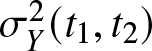 $\sigma^{2}_Y(t_1,t_2)$ be the mean and variance of Y in the interval $(t_1,t_2)$ both assumed to be finite on $\mathbb{R}$. Then, for all $(t_{1},t_{2})\in D$,
 \begin{equation*}
\mathcal{VI}_K(X_{t_1,t_2},Y_{t_1,t_2}) \geq \sigma_Y^2(t_1,t_2) \cdot\left(E\left[\omega^{\prime}_{Y_{t_1,t_2}}(Y_{t_1,t_2})\right]\right )^{2},
\end{equation*}
\begin{equation*}
\mathcal{VI}_K(X_{t_1,t_2},Y_{t_1,t_2}) \geq \sigma_Y^2(t_1,t_2) \cdot\left(E\left[\omega^{\prime}_{Y_{t_1,t_2}}(Y_{t_1,t_2})\right]\right )^{2},
\end{equation*} where  $\omega^{\prime}_{Y_{t_1,t_2}}(x)$ is the derivative of the function $\omega_{Y_{t_1,t_2}}(x)$ which is defined by
 \begin{equation*}
\sigma^2_Y(t_1,t_2)\omega_{Y_{t_1,t_2}}(x)g_{t_1,t_2}(x) = \int_{0}^{x} [m_Y(t_1,t_2) - z]g_{t_1,t_2}(z)dz, x \gt 0.
\end{equation*}
\begin{equation*}
\sigma^2_Y(t_1,t_2)\omega_{Y_{t_1,t_2}}(x)g_{t_1,t_2}(x) = \int_{0}^{x} [m_Y(t_1,t_2) - z]g_{t_1,t_2}(z)dz, x \gt 0.
\end{equation*}Proof. In line with Theorem 2.3 of Sharma and Kundu [Reference Sharma and Kundu21], the proof follows.
The significance of this bound lies in its ability to be estimated using the doubly truncated mean and variance of the random variable Y, based on its pdf. Notably, this bound is independent of the df of X, making it a robust and versatile estimation method. This approach simplifies the purpose, making it both time-efficient and practical for situations where exact expressions are difficult to derive. Additionally, it reduces computational effort and enhances versatility, allowing its application to a wide range of distributions and analytical cases. In cases where it is difficult to evaluate the doubly truncated varinaccuracy, a suitable upper bound to it, given in the following theorem may be useful. Before it, note that
 \begin{equation*}
\mathcal{I}_K^{w}(X_{t_1,t_2},Y_{t_1,t_2})=
-\int_{t_1}^{t_2}x\frac{f(x)}{F(t_2)-F(t_1)}\log{\frac{g(x)}{G(t_2)-G(t_1)}}dx
\end{equation*}
\begin{equation*}
\mathcal{I}_K^{w}(X_{t_1,t_2},Y_{t_1,t_2})=
-\int_{t_1}^{t_2}x\frac{f(x)}{F(t_2)-F(t_1)}\log{\frac{g(x)}{G(t_2)-G(t_1)}}dx
\end{equation*}and
 \begin{equation*}
m_X(t_1,t_2)=E[X|t_1 \lt X \lt t_2], ~~~(t_1,t_2)\in D;
\end{equation*}
\begin{equation*}
m_X(t_1,t_2)=E[X|t_1 \lt X \lt t_2], ~~~(t_1,t_2)\in D;
\end{equation*} where  $\mathcal{I}_K^{w}(X_{t_1,t_2},Y_{t_1,t_2})$ is the weighted doubly truncated inaccuracy measure (cf. [Reference Kundu13]) and $m_X(t_1,t_2)$ is the generalized conditional mean of X in $(t_1,t_2)$, respectively.
Theorem 2.6. Let the pdf of the random variable Y fulfil
 \begin{equation}
e^{-ax-b}\leq g(x) \leq 1,~~~\forall x\geq 0,~\text{where}~a \gt 0,b\geq 0.
\end{equation}
\begin{equation}
e^{-ax-b}\leq g(x) \leq 1,~~~\forall x\geq 0,~\text{where}~a \gt 0,b\geq 0.
\end{equation} Then,  $\forall (t_1,t_2)\in D$, we have
 \begin{eqnarray*}
\mathcal{VI}_K(X_{t_1,t_2},Y_{t_1,t_2}) &\leq& a\left[\mathcal{I}_K^{w}(X_{t_1,t_2},Y_{t_1,t_2})+m_X(t_1,t_2)\cdot\Lambda_Y(t_1,t_2)\right]\\
&& +b\left[\Lambda_Y(t_1,t_2)+\mathcal{I}_K(X_{t_1,t_2},Y_{t_1,t_2})\right]
-\left[\Lambda_Y(t_1,t_2)+\mathcal{I}_K(X_{t_1,t_2},Y_{t_1,t_2})\right]^2.
\end{eqnarray*}
\begin{eqnarray*}
\mathcal{VI}_K(X_{t_1,t_2},Y_{t_1,t_2}) &\leq& a\left[\mathcal{I}_K^{w}(X_{t_1,t_2},Y_{t_1,t_2})+m_X(t_1,t_2)\cdot\Lambda_Y(t_1,t_2)\right]\\
&& +b\left[\Lambda_Y(t_1,t_2)+\mathcal{I}_K(X_{t_1,t_2},Y_{t_1,t_2})\right]
-\left[\Lambda_Y(t_1,t_2)+\mathcal{I}_K(X_{t_1,t_2},Y_{t_1,t_2})\right]^2.
\end{eqnarray*}Proof. Under the assumption (2.16), we write Eq. (2.6) as
 \begin{equation}
\mathcal{VI}_K(X_{t_1,t_2},Y_{t_1,t_2})\leq -\int_{t_1}^{t_2}(a x+b) \frac{f(x)}{F(t_2)-F(t_1)}\log{g(x)}dx-[\mathcal{I}_K(X_{t_1,t_2},Y_{t_1,t_2})+\Lambda_Y(t_1,t_2)]^2.
\end{equation}
\begin{equation}
\mathcal{VI}_K(X_{t_1,t_2},Y_{t_1,t_2})\leq -\int_{t_1}^{t_2}(a x+b) \frac{f(x)}{F(t_2)-F(t_1)}\log{g(x)}dx-[\mathcal{I}_K(X_{t_1,t_2},Y_{t_1,t_2})+\Lambda_Y(t_1,t_2)]^2.
\end{equation}Further, we may write
 \begin{equation}
-\int_{t_1}^{t_2}x\frac{f(x)}{F(t_2)-F(t_1)}\log{g(x)}dx= [m_X(t_1,t_2)\Lambda_Y(t_1,t_2)+ \mathcal{I}_K^{w}(X_{t_1,t_2},Y_{t_1,t_2})].
\end{equation}
\begin{equation}
-\int_{t_1}^{t_2}x\frac{f(x)}{F(t_2)-F(t_1)}\log{g(x)}dx= [m_X(t_1,t_2)\Lambda_Y(t_1,t_2)+ \mathcal{I}_K^{w}(X_{t_1,t_2},Y_{t_1,t_2})].
\end{equation}Also, Eq. (1.3) can be written as
 \begin{equation}
-\int_{t_1}^{t_2}\frac{f(x)}{F(t_2)-F(t_1)}\log{g(x)}dx=[\Lambda_Y(t_1,t_2)+\mathcal{I}_K(X_{t_1,t_2},Y_{t_1,t_2})].
\end{equation}
\begin{equation}
-\int_{t_1}^{t_2}\frac{f(x)}{F(t_2)-F(t_1)}\log{g(x)}dx=[\Lambda_Y(t_1,t_2)+\mathcal{I}_K(X_{t_1,t_2},Y_{t_1,t_2})].
\end{equation}Eventually, the expression follows once we substitute (2.18) and (2.19) in (2.17).
The key significance of this bound is that it relies solely on the doubly truncated mean of the random variable X in time interval  $(t_1,t_2)$, along with the doubly truncated inaccuracy and its weighted form evaluted for X and Y, for its evaluation. By identifying the upper bound on interval varinaccuracy, it ensures that the measure remains within acceptable thresholds, offering stability and limitation of error. We illustrate the above theorem in the example below.
Example 2.4. Consider X and Y from Example 2.1(i), where η = 1. Then one may evaluate
 \begin{equation*}
m_X(t_1,t_2)=\frac{1}{\lambda}+\frac{t_1e^{-\lambda t_1}-t_2e^{-\lambda t_2}}{e^{-\lambda t_1}-e^{-\lambda t_2}}
\end{equation*}
\begin{equation*}
m_X(t_1,t_2)=\frac{1}{\lambda}+\frac{t_1e^{-\lambda t_1}-t_2e^{-\lambda t_2}}{e^{-\lambda t_1}-e^{-\lambda t_2}}
\end{equation*}and
 \begin{eqnarray*}
\mathcal{I}_K^{w}(X_{t_1,t_2},Y_{t_1,t_2})&=&\frac{t_1e^{-\lambda t_1}-t_2e^{-\lambda t_2}}{e^{-\lambda t_1}-e^{-\lambda t_2}}\log{(e^{-t_1}-e^{-t_2})}+\frac{\log{(e^{-t_1}-e^{-t_2})}}{\lambda} \\
&&+ \frac{(t_1^2\lambda^2+2\lambda t_1+2)e^{-\lambda t_1}-(t_2^2\lambda^2+2\lambda t_2+2)e^{-\lambda t_2}}{\lambda^2(e^{-\lambda t_1}-e^{-\lambda t_2})}.
\end{eqnarray*}
\begin{eqnarray*}
\mathcal{I}_K^{w}(X_{t_1,t_2},Y_{t_1,t_2})&=&\frac{t_1e^{-\lambda t_1}-t_2e^{-\lambda t_2}}{e^{-\lambda t_1}-e^{-\lambda t_2}}\log{(e^{-t_1}-e^{-t_2})}+\frac{\log{(e^{-t_1}-e^{-t_2})}}{\lambda} \\
&&+ \frac{(t_1^2\lambda^2+2\lambda t_1+2)e^{-\lambda t_1}-(t_2^2\lambda^2+2\lambda t_2+2)e^{-\lambda t_2}}{\lambda^2(e^{-\lambda t_1}-e^{-\lambda t_2})}.
\end{eqnarray*}Thus, applying Theorem 2.6 for a = 1 and b = 1, we have for λ > 0
 \begin{eqnarray*}
\mathcal{VI}_K(X_{t_1,t_2},Y_{t_1,t_2}) &\leq& \frac{1}{\lambda}\left(\frac{1}{\lambda}+1\right)+\frac{t_1^2e^{-\lambda t_1}-t_2^2e^{-\lambda t_2}}{e^{-\lambda t_1}-e^{-\lambda t_2}}-\left(\frac{t_1e^{-\lambda t_1}-t_2e^{-\lambda t_2}}{e^{-\lambda t_1}-e^{-\lambda t_2}}\right)^2 \\
&&+\frac{t_1e^{-\lambda t_1}-t_2e^{-\lambda t_2}}{e^{-\lambda t_1}-e^{-\lambda t_2}}.
\end{eqnarray*}
\begin{eqnarray*}
\mathcal{VI}_K(X_{t_1,t_2},Y_{t_1,t_2}) &\leq& \frac{1}{\lambda}\left(\frac{1}{\lambda}+1\right)+\frac{t_1^2e^{-\lambda t_1}-t_2^2e^{-\lambda t_2}}{e^{-\lambda t_1}-e^{-\lambda t_2}}-\left(\frac{t_1e^{-\lambda t_1}-t_2e^{-\lambda t_2}}{e^{-\lambda t_1}-e^{-\lambda t_2}}\right)^2 \\
&&+\frac{t_1e^{-\lambda t_1}-t_2e^{-\lambda t_2}}{e^{-\lambda t_1}-e^{-\lambda t_2}}.
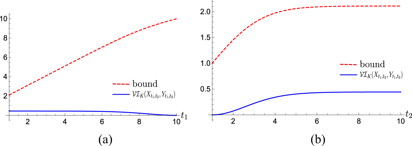
\end{eqnarray*} As a particular case, let λ = 1.5 and  $(t_1,t_2)\in D:=[1,10]$, then Figure 2 verifies the corresponding doubly truncated varinaccuracy along with the above obtained bound with respect to both t 1 and t 2, keeping the other fixed.
3. Simulation study and data analysis
This section introduces an estimator of the doubly truncated varinaccuracy taking into account the nonparametric estimation of distributions to examine the effect of t 1 and t 2 on it. The performance of the estimator have been evaluated. Moreover, the study is applied on two real data sets to validate our observations of simulation.
3.1. Simulation analysis
In this part, we propose an estimator of the interval varinaccuracy. Since nonparametric estimation are known to have the upper hand over parametric estimation in terms of robustness, flexibility from the underlying distribution, fewer assumption needs and other factors, we consider our estimator for nonparametric techniques used in statistical distribution theory. Furthermore, we demonstrate the performance of the proposed estimator by carrying out a simulation analysis taking samples from two different distributions and study the resulting variation in the similarity for different time points t 1 and t 2. The analysis is further validated using real data sets. Given that the generalized exponential distribution (GED) and Weibull distribution (WD) fit the data well, these distributions are selected for the simulation. Let X has GED given by df  $F(x)=\left(1-\exp(-\lambda x)\right)^\alpha$, where α and λ are the shape and scale parameters, respectively and Y has WD with shape parameter k and scale parameter σ given by df $G(x)=1-\exp\left(-\left(x/\sigma\right)^k\right)$. Recall that kernel-smoothed estimators provide flexibility by avoiding parametric assumptions, deliver smooth and continuous estimates and adapt to local data variations. They are robust to random fluctuations, handles distribution shape and visually interpretable, aiding in understanding the behavior of the data distribution. Given the better performance of the smoothed estimators in comparison to non-smoothed estimators, we use kernel-smoothed estimator $\hat{\mathcal{F}}_n(x)$ (cf. [Reference Parkash and Kakkar18]) for the nonparametric estimation of the assumed distributions given as
Plot of bound and  $\mathcal{VI}_K(X_{t_1,t_2},Y_{t_1,t_2})$ (Theorem 2.6).
 \begin{equation*}
\hat{\mathcal{F}}_n(x)=\frac{1}{n}\sum_{i=1}^{n}L\left(\frac{x-X_i}{h}\right),
\end{equation*}
\begin{equation*}
\hat{\mathcal{F}}_n(x)=\frac{1}{n}\sum_{i=1}^{n}L\left(\frac{x-X_i}{h}\right),
\end{equation*} for a given random sample  $X_i, i=1,2,...,n$, provided df $L(\cdot)$ of the positive kernel K, that is, $L(v)=\int_{0}^{+\infty}K(t)dt$, along with bandwidth of parameter h. Note that the kernel function $K(v)=\frac{1}{\sqrt{2\pi}}\exp\left(-\frac{v^2}{2}\right)$ known as Gaussian kernel function is used for the above estimation and the bandwidth h was determined using the Sheather–Jones method for kernel density estimation. Let us assume $\hat{X}$ and $\hat{Y}$ to relate with $\hat{F}_n(\cdot)$ and $\hat{G}_n(\cdot)$, respectively. We now use the expression given in Eq. (2.5) to introduce the estimator for the doubly truncated varinaccuracy measure expressed as
 \begin{align}
\mathcal{\widehat{VI}}_K(\hat{X}_{t_1,t_2},\hat{Y}_{t_1,t_2})&=
\int_{t_1}^{t_2}\frac{\hat{f}_n(x)}{\hat{F}_n(t_2)-\hat{F}_n(t_1)}
\left(\log{\frac{\hat{g}_n(x)}{\hat{G}_n(t_2)-\hat{G}_n(t_1)}}\right)^2dx \nonumber\\
&\quad -\left[\int_{t_1}^{t_2}\frac{\hat{f}_n(x)}{\hat{F}_n(t_2)-\hat{F}_n(t_1)}
\log{\frac{\hat{g}_n(x)}{\hat{G}_n(t_2)-\hat{G}_n(t_1)}}dx\right]^2,
\end{align}
\begin{align}
\mathcal{\widehat{VI}}_K(\hat{X}_{t_1,t_2},\hat{Y}_{t_1,t_2})&=
\int_{t_1}^{t_2}\frac{\hat{f}_n(x)}{\hat{F}_n(t_2)-\hat{F}_n(t_1)}
\left(\log{\frac{\hat{g}_n(x)}{\hat{G}_n(t_2)-\hat{G}_n(t_1)}}\right)^2dx \nonumber\\
&\quad -\left[\int_{t_1}^{t_2}\frac{\hat{f}_n(x)}{\hat{F}_n(t_2)-\hat{F}_n(t_1)}
\log{\frac{\hat{g}_n(x)}{\hat{G}_n(t_2)-\hat{G}_n(t_1)}}dx\right]^2,
\end{align} where  $\hat{f}_n(\cdot)$ and $\hat{g}_n(\cdot)$ are the kernel-density estimates obtained from n samples of generalized exponential and WDs with corresponding dfs as $\hat{F}_n(\cdot)$ and $\hat{G}_n(\cdot)$, respectively. For different time points t 1 and t 2, the estimated values of $\mathcal{\widehat{VI}}_K(\hat{X}_{t_1,t_2},\hat{Y}_{t_1,t_2})$ may be computed from (3.20).
Using the above estimator, we perform a Monte-Carlo simulation study. The analysis begins by considering random samples Xi and Yi for  $i=1,2,...,n$, generated from GED with $(\alpha,\lambda)=(4,0.5)$ and WD having $(k,\sigma)=(2,6.5)$, respectively, using R-software. The estimated values of the interval varinaccuracy for different truncation limits $(t_1,t_2)$ have been computed on performing 100 simulations respectively, of size n (50, 100, 200, 500 and 1,000). The calculated average of these 100 values is treated as the final estimated value of the interval varinaccuracy. To analyze the performance of the proposed estimator, bias and mean squared error (MSE) are also computed. For each case, bias and MSE are computed by comparing the estimator results to the true values using repeated simulations and average value obtained is treated as its final value. In Table 1, the estimates along with the observed value, bias and MSE are presented. In general, it is observed that the estimated values of the interval varinaccuracy increase with increase in size of the interval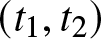 $(t_1,t_2)$. In other words, we may state that the varinaccuracy decreases when the observation is confined to a shrinking interval. The outcomes of the simulation study show decrease in the absolute values of bias and MSE as the sample size n increases, which validate the performance and consistency of the proposed estimator. In conclusion, the estimates are nearly unbiased on considering sufficiently large sample sizes. Following the insights gained from the simulation results, we now apply the estimator to the real data sets to assess its practical effectiveness and verify its performance.
Estimated values of  $\mathcal{\widehat{VI}}_K(\hat{X}_{t_1,t_2},\hat{Y}_{t_1,t_2})$ with true value $\mathcal{VI}_K(X_{t_1,t_2},Y_{t_1,t_2})$ along with the Bias and MSE for different time intervals $(t_1,t_2)$ obtained for sample sizes $n=50, 100, 200, 500 ~\text{and}~1000$.

3.2. Real data sets
In this part, we apply the above methodology to two real data sets. The above simulation results served as a preliminary test of the estimator’s performance to assess the estimator’s performance allowing us to observe its behavior under controlled conditions, such as different distributions and time points. The real data sets here are used to validate the findings from the simulation, ensuring the estimator’s practical applicability and reliability in real-world scenarios. We choose the data sets of mortality rates due to COVID-19 for Mexico and Italy reproduced from https://covid19.who.int/region/country and recorded from 4 March to 20 July 2020 and 27 February to 27 April 2020, respectively, considering the peak of the pandemic. These specific datasets are chosen because they align well with the assumptions made in the simulations, providing a realistic test case for the estimator. The data sets have been given below.
Mexico: 8.826, 6.105, 10.383, 7.267, 13.220, 6.015, 10.855, 6.122, 10.685, 10.035, 5.242, 7.630, 14.604, 7.903, 6.327, 9.391, 14.962, 4.730, 3.215, 16.498, 11.665, 9.284, 12.878, 6.656, 3.440, 5.854, 8.813, 10.043, 7.260, 5.985, 4.424, 4.344, 5.143, 9.935, 7.840, 9.550, 6.968, 6.370, 3.537, 3.286, 10.158, 8.108, 6.697, 7.151, 6.560, 2.988, 3.336, 6.814, 8.325, 7.854, 8.551, 3.228, 3.499, 3.751, 7.486, 6.625, 6.140, 4.909, 4.661, 1.867, 2.838, 5.392, 12.042, 8.696, 6.412, 3.395, 1.815, 3.327, 5.406, 6.182, 4.949, 4.089, 3.359, 2.070, 3.298, 5.317, 5.442, 4.557, 4.292, 2.500, 6.535, 4.648, 4.697, 5.459, 4.120, 3.922, 3.219, 1.402, 2.438, 3.257, 3.632, 3.233, 3.027, 2.352, 1.205, 2.077, 3.778, 3.218, 2.926, 2.601, 2.065, 1.041, 1.800, 3.029, 2.058, 2.326, 2.506 and 1.923.
Italy: 4.571, 7.201, 3.606, 8.479, 11.410, 8.961, 10.919, 10.908, 6.503, 18.474, 11.010, 17.337, 16.561, 13.226, 15.137, 8.697, 15.787, 13.333, 11.822, 14.242, 11.273, 14.330, 16.046, 11.950, 10.282, 11.775, 10.138, 9.037, 12.396, 10.644, 8.646, 8.905, 8.906, 7.407, 7.445, 7.214, 6.194, 4.640, 5.452, 5.073, 4.416, 4.859, 4.408, 4.639, 3.148, 4.040, 4.253, 4.011, 3.564, 3.827, 3.134, 2.780, 2.881, 3.341, 2.686, 2.814, 2.508, 2.450 and 1.518.
We observe the fitting of following distributions (D) to the above data sets using R-software given in order of better fit.
(i) The GED
 \begin{equation*}
f(x)=\alpha\lambda e^{-\lambda x}(1-e^{-\lambda x})^{\alpha-1},~~~\alpha,\lambda \gt 0, x \gt 0;
\end{equation*}
\begin{equation*}
f(x)=\alpha\lambda e^{-\lambda x}(1-e^{-\lambda x})^{\alpha-1},~~~\alpha,\lambda \gt 0, x \gt 0;
\end{equation*} for  $(\alpha,\lambda)=(3.996542,0.3619396)$ and $(\alpha,\lambda)=(3.488966,0.2399844)$ to the data sets of Mexico and Italy, respectively.
(ii) The WD
 \begin{equation*}
f(x)=(a/\sigma) (x/\sigma)^{a-1}e^{-(x/\sigma)^a};~~~\sigma,a \gt 0,x \gt 0;
\end{equation*}
\begin{equation*}
f(x)=(a/\sigma) (x/\sigma)^{a-1}e^{-(x/\sigma)^a};~~~\sigma,a \gt 0,x \gt 0;
\end{equation*} with parameters  $(a,\sigma)=(1.896812,6.520891)$ and $(a,\sigma)=(1.9271,9.232718)$ to the data sets of Mexico and Italy, respectively.
The maximum log-likelihood (- $\ln{L}$), Akaike Information Criterion (AIC), Bayesian Information Criterion (BIC), Kolmogorov–Smirnov (K–S) distance and its associated p-value obtained for the data sets of Mexico and Italy are listed in Tables 2 and 3, respectively.
Results of the fitted distribution for Mexico data set.

Results of the fitted distribution for Italy data set.

Furthermore, we apply the above estimation process using (3.20) taking  $\hat{X}$ as the nonparametric density estimate obtained from the complete data set and $\hat{Y}$ to be density estimate from the samples lying between different $(t_1,t_2)$. MSE and bias have also been computed for the true value of the doubly truncated varinaccuracy between the above fitted distributions evaluated in the corresponding interval $(t_1,t_2)$. The results obtained from the real data analysis are presented in the tables below, providing a detailed comparison of the estimator’s performance in real data against the insights gained from the simulation analysis. Tables 4 and 5 show the observed values and true values of the interval varinaccuracy for different time points $(t_1,t_2)$ along with the corresponding bias and MSE for the data sets of Mexico and Italy, respectively. The bias values here indicate the extent to which the estimator systematically deviates from the true value, with smaller bias suggesting a more accurate estimator. The MSE values, which combine both bias and variance, show the overall precision of the estimator; lower MSE values indicate that the estimator is both consistent and efficient, thus validating its performance for real data sets. It is clear from Tables 4 and 5 that as the number of sample points in $(t_1,t_2)$ increases, absolute values of bias and MSE decreases, that is, estimates are closer to the actual value. Specifically, the table shows that as the sample size increases in the real data sets, the estimated values of interval varinaccuracy approach those obtained from the fitted distributions within the respective intervals. A similar trend was observed in the simulation analysis as well. However, interval varinaccuracy shows different patterns across the two models. In the first model, it increases with a fixed t 1 and increasing t 2, while the second model displays a non-monotonic behavior of the interval varinaccuracy. Regarding performance comparison, as the sample size increases, both bias and MSE decrease for both the Mexico and Italy data sets, indicating improved accuracy of the estimator in both the cases. This observation suggests that the models become more reliable with larger sample sizes. Therefore, the results of the simulation study are verified by the above real data sets. $\mathcal{\widehat{VI}}_K(\hat{X}_{t_1,t_2},\hat{Y}_{t_1,t_2})$, $\mathcal{VI}_K(X_{t_1,t_2},Y_{t_1,t_2})$ with bias and MSE for Mexico data set.
 $\mathcal{\widehat{VI}}_K(\hat{X}_{t_1,t_2},\hat{Y}_{t_1,t_2})$, $\mathcal{VI}_K(X_{t_1,t_2},Y_{t_1,t_2})$ with bias and MSE for Italy data set.

4. Interval varinaccuracy, proportional hazard and reversed hazard rate models (PHRM and PRHRM) and applications
Kerridge’s inaccuracy measure plays a significant role in evaluating the performance of the PHRM (PRHRM) in survival analysis. The interval inaccuracy measure under PHRM (PRHRM) examined by Kundu and Nanda [Reference Kundu and Nanda15] is found to be useful in characterization of certain distributions. In other words, the interval inaccuracy measure not only assesses how well the PHRM (PRHRM) fits the observed survival data but also identifies the underlying distribution of it in certain cases. It thus provides valuable insights into the model fit and comparison to alternate models. We intend to evaluate the corresponding interval varinaccuracy using (2.5) under PHRM (PRHRM), which may further enhance the study of inaccuracy under it and may be useful to understand the behavior of the underlying distribution in terms of dispersion around the inaccuracy. Studying both the PHRM and PRHRM together is crucial, especially for interval lifetime data, as they offer complementary perspectives on reliability and survival analysis. The PHRM focuses on the future risk of failure, given survival up to a certain time, making it ideal for predicting and assessing ongoing risks. In contrast, the PRHRM examines the likelihood of past failures, given survival at a specific time, providing insights into the tail behavior and past reliability. For interval lifetime data, where exact failure times are unknown but fall within specified intervals, considering both models helps capture the forward and backward dynamics of the data. This dual approach ensures a more comprehensive understanding of system behavior, enhances model accuracy and supports better decision-making in maintenance planning, risk assessment and reliability optimization. Recall that PHRM (cf. [Reference Cox5]) is given by
 \begin{equation*}
\overline{G}(t)=[\overline{F}(t)]^\theta,~~~\theta \gt 0;
\end{equation*}
\begin{equation*}
\overline{G}(t)=[\overline{F}(t)]^\theta,~~~\theta \gt 0;
\end{equation*} where  $\overline{G}(\cdot)$ and $\overline{F}(\cdot)$ are the sfs of X and Y, respectively. Under this model, the failure rate functions $\lambda_X(\cdot)$ and $\lambda_Y(\cdot)$ of random variables X and Y, respectively, are related as
 \begin{equation*}
\lambda_Y(t)=\theta\lambda_X(t),
\end{equation*}
\begin{equation*}
\lambda_Y(t)=\theta\lambda_X(t),
\end{equation*} where  $\lambda_X(t)=f(t)/\overline{F}(t)$ and $\lambda_Y(t)=g(t)/\overline{G}(t)$. The failure rate function describes the instantaneous failure rate of a system subject to survival up to time t and is crucial in understanding the failure rates of a system over time.
The PHRM in information theory is significant as it quantifies how the hazard rate changes over time based on external factors. By modeling these hazards in terms of uncertainty, it allows for the measurement of information gain over time, reducing uncertainty in predictions. This is especially useful for understanding how the distribution of event times can be more accurately predicted, enhancing decision-making under uncertainty. Moreover, the hazard ratio θ is a valuable tool in reliability engineering for understanding how various factors affect the lifetime and failure probability of systems, allowing for more informed design and decisions. The interval inaccuracy under PHRM is calculated as
 \begin{align}
\mathcal{I}_K(X_{t_1,t_2},Y_{t_1,t_2})&= \theta-\log{\theta}+\log{\left(\overline{F}^\theta(t_1)-\overline{F}^\theta(t_2)\right)}+\theta \frac{\overline{F}(t_2)\log{\overline{F}(t_2)}-\overline{F}(t_1)\log{\overline{F}(t_1)}}
{\overline{F}(t_1)-\overline{F}(t_2)}\nonumber\\
&\quad -\int_{t_1}^{t_2}\frac{f(x)}{\overline{F}(t_1)-\overline{F}(t_2)}\log{\lambda_X(x)}dx.
\end{align}
\begin{align}
\mathcal{I}_K(X_{t_1,t_2},Y_{t_1,t_2})&= \theta-\log{\theta}+\log{\left(\overline{F}^\theta(t_1)-\overline{F}^\theta(t_2)\right)}+\theta \frac{\overline{F}(t_2)\log{\overline{F}(t_2)}-\overline{F}(t_1)\log{\overline{F}(t_1)}}
{\overline{F}(t_1)-\overline{F}(t_2)}\nonumber\\
&\quad -\int_{t_1}^{t_2}\frac{f(x)}{\overline{F}(t_1)-\overline{F}(t_2)}\log{\lambda_X(x)}dx.
\end{align}Similarly, PRHRM (cf. [Reference Gupta and Gupta8]) is a key framework in reliability and survival analysis, offering insights into past failure likelihoods and tail behaviors of lifetimes. It enables comparative studies between populations or systems through a proportional structure, supporting diverse applications like risk modeling and maintenance planning. In information theory, the PRHRM connects to uncertainty measure, making it valuable for understanding reliability and information flow in complex systems. The PRHRM is given by
 \begin{equation*}
G(t)=[F(t)]^\beta, ~~~\beta \gt 0;
\end{equation*}
\begin{equation*}
G(t)=[F(t)]^\beta, ~~~\beta \gt 0;
\end{equation*} where  $F(\cdot)$ and $G(\cdot)$ are the dfs of X and Y, respectively. The proportionality constant β in the PRHRM quantifies the relative tail behaviors of two distributions, making it a useful tool for comparing systems or populations with different long-term reliability or survival characteristics. The reversed hazard function measures the likelihood of past failure, given survival up to a certain time, making it essential for analyzing tail behaviors of lifetime distributions and understanding system reliability in retrospective scenarios. Recall that the reversed hazard rate function of X is defined as $\mu_X(t)=f(t)/F(t)$. The reversed hazard rate functions of X and Y under this model are related by
 \begin{equation*}
\mu_{Y}(x)=\beta\mu_{X}(x),
\end{equation*}
\begin{equation*}
\mu_{Y}(x)=\beta\mu_{X}(x),
\end{equation*} where  $\mu_Y(\cdot)$ is the reversed hazard rate function of Y. The reversed hazard rate function gives the instantaneous rate of failure at time t given that failure occurred at or before time t. The interval inaccuracy under PRHRM is evaluated as
 \begin{align}
\mathcal{I}_K(X_{t_1,t_2},Y_{t_1,t_2})&= \beta-\log{\beta}+\log{\left(F^\beta(t_2)-F^\beta(t_1)\right)}+\beta \frac{F(t_2)\log{F(t_2)}-F(t_1)\log{F(t_1)}}
{F(t_2)-F(t_1)}\nonumber\\
&\quad -\int_{t_1}^{t_2}\frac{f(x)}{F(t_2)-F(t_1)}\log{\mu_X(x)}dx.
\end{align}
\begin{align}
\mathcal{I}_K(X_{t_1,t_2},Y_{t_1,t_2})&= \beta-\log{\beta}+\log{\left(F^\beta(t_2)-F^\beta(t_1)\right)}+\beta \frac{F(t_2)\log{F(t_2)}-F(t_1)\log{F(t_1)}}
{F(t_2)-F(t_1)}\nonumber\\
&\quad -\int_{t_1}^{t_2}\frac{f(x)}{F(t_2)-F(t_1)}\log{\mu_X(x)}dx.
\end{align}To analyze the underlying distribution more accurately in the given range, it is recommended to study the interval varinaccuracy therein. The below theorem evaluates the dispersion around interval inaccuracy under PHRM.
Theorem 4.1. Under the above assumption of PHRM, the interval varinaccuracy for all  $(t_1,t_2)\in D$ may be evaluated as
 \begin{align*}
\mathcal{VI}_K(X_{t_1,t_2},Y_{t_1,t_2}) &= \theta^2 + \textrm{Var}[\log{\lambda_X(x)}|t_1 \lt X \lt t_2]-\theta^2\frac{\overline{F}(t_1)\overline{F}(t_2)\left(\log{\frac{\overline{F}(t_1)}
{\overline{F}(t_2)}}\right)^2}{(\overline{F}(t_1)-\overline{F}(t_2))^2} \\
&\quad +2\theta \left[1-\frac{\overline{F}(t_1)\log{\overline{F}(t_1)}-\overline{F}(t_2)
\log{\overline{F}(t_2)}}{\overline{F}(t_1)-\overline{F}(t_2)} \right]E[\log{\lambda_X(x)}|t_1 \lt X \lt t_2]\\
&\quad +2\theta \cdot E[\log{\overline{F}(x)}\cdot\log{\lambda_X(x)}|t_1 \lt X \lt t_2].
\end{align*}
\begin{align*}
\mathcal{VI}_K(X_{t_1,t_2},Y_{t_1,t_2}) &= \theta^2 + \textrm{Var}[\log{\lambda_X(x)}|t_1 \lt X \lt t_2]-\theta^2\frac{\overline{F}(t_1)\overline{F}(t_2)\left(\log{\frac{\overline{F}(t_1)}
{\overline{F}(t_2)}}\right)^2}{(\overline{F}(t_1)-\overline{F}(t_2))^2} \\
&\quad +2\theta \left[1-\frac{\overline{F}(t_1)\log{\overline{F}(t_1)}-\overline{F}(t_2)
\log{\overline{F}(t_2)}}{\overline{F}(t_1)-\overline{F}(t_2)} \right]E[\log{\lambda_X(x)}|t_1 \lt X \lt t_2]\\
&\quad +2\theta \cdot E[\log{\overline{F}(x)}\cdot\log{\lambda_X(x)}|t_1 \lt X \lt t_2].
\end{align*}Proof. Under PHRM, the first term in RHS of Eq. (2.5) is written as
 \begin{align*}
&\int_{t_1}^{t_2}\frac{f(x)}{\overline{F}(t_1)-\overline{F}(t_2)}\left(\log{\frac{\theta[\overline{F}(x)]^\theta \lambda_X(x)}{\overline{F}^\theta(t_1)-\overline{F}^\theta(t_2)}}\right)^2dx \\
&=\int_{t_1}^{t_2}\frac{f(x)}{\overline{F}(t_1)-\overline{F}(t_2)}\left(\log{\theta}+\theta\log{\overline{F}(x)}+
\log{\lambda_X(x)}-\log{(\overline{F}^\theta(t_1)-\overline{F}^\theta(t_2))}\right)^2dx
\end{align*}
\begin{align*}
&\int_{t_1}^{t_2}\frac{f(x)}{\overline{F}(t_1)-\overline{F}(t_2)}\left(\log{\frac{\theta[\overline{F}(x)]^\theta \lambda_X(x)}{\overline{F}^\theta(t_1)-\overline{F}^\theta(t_2)}}\right)^2dx \\
&=\int_{t_1}^{t_2}\frac{f(x)}{\overline{F}(t_1)-\overline{F}(t_2)}\left(\log{\theta}+\theta\log{\overline{F}(x)}+
\log{\lambda_X(x)}-\log{(\overline{F}^\theta(t_1)-\overline{F}^\theta(t_2))}\right)^2dx
\end{align*} \begin{align*}
&= (\log{\theta})^2+\left(\log{\overline{F}^\theta(t_1)-\overline{F}^\theta(t_2)}\right)^2 \\
&-2\log{\theta}\cdot\log{(\overline{F}^\theta(t_1)-\overline{F}^\theta(t_2))}
+2[\log{\theta}-\log{(\overline{F}^\theta(t_1)-\overline{F}^\theta(t_2))}]E[\log{\lambda_X(x)}|t_1 \lt X \lt t_2] \\
&+\theta^2\left[\frac{\overline{F}(t_1)(\log{\overline{F}(t_1)})^2-\overline{F}(t_2)(\log{\overline{F}(t_2)})^2}
{\overline{F}(t_1)-\overline{F}(t_2)}-2\left(\frac{\overline{F}(t_1)
\log{\overline{F}(t_1)}-\overline{F}(t_2)\log{\overline{F}(t_2)}}
{\overline{F}(t_1)-\overline{F}(t_2)}\right)+2 \right]\\
&+ 2\theta[\log{\theta}-\log{(\overline{F}^\theta(t_1)-\overline{F}^\theta(t_2))}]\left(\frac{\overline{F}(t_1)
\log{\overline{F}(t_1)}-\overline{F}(t_2)\log{\overline{F}(t_2)}}
{\overline{F}(t_1)-\overline{F}(t_2)}-1\right)\\
& +E[(\log{\lambda_X(x)})^2|t_1 \lt X \lt t_2]
+2\theta E[\log{\overline{F}(x)}\cdot\log{\lambda_X(x)}|t_1 \lt X \lt t_2].
\end{align*}
\begin{align*}
&= (\log{\theta})^2+\left(\log{\overline{F}^\theta(t_1)-\overline{F}^\theta(t_2)}\right)^2 \\
&-2\log{\theta}\cdot\log{(\overline{F}^\theta(t_1)-\overline{F}^\theta(t_2))}
+2[\log{\theta}-\log{(\overline{F}^\theta(t_1)-\overline{F}^\theta(t_2))}]E[\log{\lambda_X(x)}|t_1 \lt X \lt t_2] \\
&+\theta^2\left[\frac{\overline{F}(t_1)(\log{\overline{F}(t_1)})^2-\overline{F}(t_2)(\log{\overline{F}(t_2)})^2}
{\overline{F}(t_1)-\overline{F}(t_2)}-2\left(\frac{\overline{F}(t_1)
\log{\overline{F}(t_1)}-\overline{F}(t_2)\log{\overline{F}(t_2)}}
{\overline{F}(t_1)-\overline{F}(t_2)}\right)+2 \right]\\
&+ 2\theta[\log{\theta}-\log{(\overline{F}^\theta(t_1)-\overline{F}^\theta(t_2))}]\left(\frac{\overline{F}(t_1)
\log{\overline{F}(t_1)}-\overline{F}(t_2)\log{\overline{F}(t_2)}}
{\overline{F}(t_1)-\overline{F}(t_2)}-1\right)\\
& +E[(\log{\lambda_X(x)})^2|t_1 \lt X \lt t_2]
+2\theta E[\log{\overline{F}(x)}\cdot\log{\lambda_X(x)}|t_1 \lt X \lt t_2].
\end{align*}On substituting the above and the expression of interval varinaccuracy under PRHM (4.21) in Eq. (2.5), the required expression of the interval varinaccuracy under PRHM is attained after some arrangements.
A similar expression of the interval varinaccuracy between X and Y under PRHRM is given in the below theorem. The proof is left out.
Theorem 4.2. Under PRHRM, the interval varinaccuracy for all  $(t_1,t_2)\in D$ is given by
 \begin{align*}
\mathcal{VI}_K(X_{t_1,t_2},Y_{t_1,t_2}) &= \beta^2 + \textrm{Var}[\log{\mu_X(x)}|t_1 \lt X \lt t_2]-\beta^2\frac{F(t_1)F(t_2)\left(\log{\frac{F(t_2)}
{F(t_1)}}\right)^2}{(F(t_2)-F(t_1))^2} \\
&\quad +2\beta \left[1-\frac{F(t_2)\log{F(t_2)}-F(t_1)
\log{F(t_1)}}{F(t_2)-F(t_1)} \right]E[\log{\mu_X(x)}|t_1 \lt X \lt t_2]\\
&\quad +2\beta \cdot E[\log{F(x)}\cdot\log{\mu_X(x)}|t_1 \lt X \lt t_2].
\end{align*}
\begin{align*}
\mathcal{VI}_K(X_{t_1,t_2},Y_{t_1,t_2}) &= \beta^2 + \textrm{Var}[\log{\mu_X(x)}|t_1 \lt X \lt t_2]-\beta^2\frac{F(t_1)F(t_2)\left(\log{\frac{F(t_2)}
{F(t_1)}}\right)^2}{(F(t_2)-F(t_1))^2} \\
&\quad +2\beta \left[1-\frac{F(t_2)\log{F(t_2)}-F(t_1)
\log{F(t_1)}}{F(t_2)-F(t_1)} \right]E[\log{\mu_X(x)}|t_1 \lt X \lt t_2]\\
&\quad +2\beta \cdot E[\log{F(x)}\cdot\log{\mu_X(x)}|t_1 \lt X \lt t_2].
\end{align*}Proof. Under the given model, we may write
 \begin{align*}
&\int_{t_1}^{t_2}\frac{f(x)}{F(t_2)-F(t_1)}\left(\log{\frac{\beta[F(x)]^\beta \mu_X(x)}{F^\beta(t_2)-F^\beta(t_1)}}\right)^2dx \\
&=\int_{t_1}^{t_2}\frac{f(x)}{F(t_2)-F(t_1)}\left(\log{\beta}+\beta\log{F(x)}+
\log{\mu_X(x)}-\log{(F^\beta(t_2)-F^\beta(t_1))}\right)^2dx.
\end{align*}
\begin{align*}
&\int_{t_1}^{t_2}\frac{f(x)}{F(t_2)-F(t_1)}\left(\log{\frac{\beta[F(x)]^\beta \mu_X(x)}{F^\beta(t_2)-F^\beta(t_1)}}\right)^2dx \\
&=\int_{t_1}^{t_2}\frac{f(x)}{F(t_2)-F(t_1)}\left(\log{\beta}+\beta\log{F(x)}+
\log{\mu_X(x)}-\log{(F^\beta(t_2)-F^\beta(t_1))}\right)^2dx.
\end{align*}Proceeding as in Theorem 4.1, we may obtain the required expression.
An application of the interval varinaccuracy measure has been presented in the following subsection using the results obtained above.
4.1. Application
Kullback [Reference Kullback and Leibler11] identified PHRM as the best alternative to the true lifetime distribution in terms of the well-known minimum discrimination information (MDI) principle. Inaccuracy under PHRM represents the overall information about the true distribution given by the model. A natural question that occurs: Is PHRM, independent of θ, a best alternative to the actual distribution? This question seeks attention and the interval varinaccuracy given in Theorem 4.1 may be functional to analyze the model and identify the appropriate value of θ at times. It is well-known that the doubly truncated inaccuracy is greater than the doubly truncated entropy measure and it reduces to the latter for θ = 1, which is its minimum value. Intuitively, there would be atleast two values of θ in the neighborhood of its minimum having the same doubly truncated inaccuracy. Thus, inaccuracy is not sufficient measure to select θ appropriately. It is therefore constructive to use interval varinaccuracy measure for its effective choice. For instance, let X have pdf
 \begin{equation*}
f(x) = \left\{\begin{array}{ll} x,
\,\,\,\,\,\, ~if~ 0 \leq x \leq 1\\
\frac{x}{3},
\,\,\,\,\, ~if~ 1 \leq x \leq 2,\end{array}\right.
\end{equation*}
\begin{equation*}
f(x) = \left\{\begin{array}{ll} x,
\,\,\,\,\,\, ~if~ 0 \leq x \leq 1\\
\frac{x}{3},
\,\,\,\,\, ~if~ 1 \leq x \leq 2,\end{array}\right.
\end{equation*} and let  $(t_1,t_2)=(0.5,1.5)$. Then its PHRM is considered to be a suitable alternative of it. From Figure 3(a), it is clear that large value of θ should not be preferred since it would result in higher inaccuracy in the specified time interval evaluated using (4.21). A magnified view of Figure 3(a) about θ = 1 is given in Figure 3(b) which shows two values of θ having the same inaccuracy in the given interval. It is therefore recommended to use the interval varinaccuracy measure for an adequate choice. Interval varinaccuracy measures the scatterness of overall information on its similarity around the inaccuracy and the value of θ which minimizes it should be preferred for the model. Figure 4 suggests θ = 0.5 to have the least varinaccuracy in the given interval. Thus, θ = 0.5 is considered as the best choice for the PHRM when varinaccuracy in the specified interval is of importance. Therefore, in choosing the finest alternative to a given distribution in some interval, its varinaccuracy must be considered for an effective model selection.
Plot of interval inaccuracy for different values of θ (PHRM) in the time interval  $[0.5,1.5]$.

Plot of interval varinaccuracy in the time interval  $[0.5,1.5]$ under PHRM for different values of $\theta\in[0,2]$. Note that the parameter of PHRM, θ is dimensionless.

5. Conclusions
In this work, we introduced the concept of interval varinaccuracy for doubly truncated random variables, providing a novel measure for quantifying uncertainty when the distribution of the observations is unknown and confined to a specific interval. A key theoretical development is the derivation of an analytical expression that relates interval varinaccuracy with interval varentropy, allowing for direct evaluation. Additionally, we explored the behavior of the proposed measure under affine transformation, strictly monotone transformations, and established theoretical bounds that are particularly useful when exact computation may be challenging or requires more effort. To substantiate the study, examples have been presented to illustrate the effectiveness of the bounds obtained. To demonstrate the practical relevance of our findings, we have introduced the interval varinaccuracy measure for the proportional hazard model and proportional reversed hazard model in order to model its parameter, providing a better approximation of the true distribution within the given interval, based on the MDI principle. An application of the interval varinaccuracy measure under the proportional hazard model is presented where the exact value of the model parameter as a best alternative to the chosen distribution is obtained. Furthermore, we developed a kernel-based nonparametric estimator of interval varinaccuracy and evaluated its performance based on simulation studies, validating the estimator’s robustness. Application of the estimator to real-world mortality data from Mexico and Italy provided further validation and emphasized the potential of the measure in practical settings.
These applications suggest that the proposed measure can significantly improve modeling of system reliability, support more informed decision-making under uncertainty and offer a flexible tool for handling incomplete or truncated data across domains. While the methodology presented is broadly applicable, certain limitations remain. Computational challenges can arise when analyzing high-dimensional or complex datasets, and practical use may require assumptions about the underlying distribution. These challenges suggest directions for future research. However, doubly truncated varinaccuracy is a generalization of left truncated and right truncated varinaccuracy measure, but potential extensions include adapting the measure to censoring, the study of varinaccuracy in k-record values, which could offer new insights.
Acknowledgements
We gratefully acknowledge our sincere gratitude to the editorial board member and the referees for their time, careful attention and valuable insights, which have significantly contributed to improving the clarity and depth of this manuscript.
Funding statement
The authors gratefully acknowledge the financial support provided by Rajiv Gandhi Institute of Petroleum Technology, India, which facilitated the initiation of this work.
Conflict of interest
On behalf of all authors, the corresponding author states that there is no conflict of interest.


 Open access

