


1. Introduction
Swarm robotics represents a groundbreaking advancement in robotics, where numerous autonomous agents work together to achieve complex tasks without central control [Reference Brambilla, Ferrante, Birattari and Dorigo1, Reference Khaldi and Cherif2]. This concept draws inspiration from natural phenomena such as ant colonies and bee swarms, demonstrating remarkable efficiency in tasks such as foraging and territory defence. Despite the potential of these robotic systems to perform complex tasks, they often face challenges in effectively integrating human input into collaborative operations. This gap underscores the critical importance of human–swarm interaction (HSI) as a specialised domain within human–robot interaction (HRI), aimed at overcoming these limitations and fostering more efficient collaboration between humans and swarms [Reference Kolling, Nunnally and Lewis3, Reference Kolling, Walker, Chakraborty, Sycara and Lewis4]. Although HSI offers flexibility in coordinating with multiple robots through interpreters compared to HRI, it presents significant challenges to achieving intuitive control while ensuring robustness, scalability, and safety. Traditional solutions for HSI leverage intermediary devices such as joysticks [Reference Nunnally, Walker, Lewis, Chakraborty and Sycara5] or virtual reality (VR) [Reference Sachidanandam, Honarvar and Diaz-Mercado6] headsets to enable precise command execution and immersive experiences for certain users. For instance, a joystick enables straightforward navigation and direction of drone swarm movements, while VR headsets allow users to interact with the robots through gestures and spatial navigation [Reference Nagi, Giusti, Gambardella and Di Caro7], offering an enhanced sense of control. However, these devices often pose accessibility limitations. Individuals with physical disabilities, such as those lacking dexterity or mobility, or those with special needs, such as deafness, dumbness, or blindness, may find these intermediary technologies difficult to use effectively [Reference Creed, Al-Kalbani, Theil, Sarcar and Williams8]. These limitations highlight the urgent need for more inclusive solutions that cater to a broader range of users.
One HSI strategy is gesture-based interactions, which presents a promising approach for enhancing interaction with robotic swarms [Reference Benabbou, Khaldi and Benslimane9, Reference Siean, Gradinaru, Gherman, Danubianu and Milici10]. This method leverages advancements in visual-based hand gesture recognition facilitated by convolutional neural networks (CNNs) and recurrent neural networks (RNNs), significantly improving both accuracy and processing speed [Reference Huu, Hong, Dang, Quoc, Bao and Minh11–Reference Wang and Sun14]. This approach aligns with broader trends in HRI that utilise uncertainty-aware AI, such as the implementation of advanced deep learning within humanoid and assistive robotics to produce adaptable actions based on recognised human intentions [Reference Gongor and Tutsoy15–Reference Tutsoy17]. However, despite these enhancements, current systems are often limited to controlling individual robots, failing to effectively manage the collective behaviour of swarms [Reference Kawatsu, Koss, Gillies, Zhao, Crossman, Purman, Stone and Dahn18, Reference Yeh, Cheng and Shen19]. While this approach has shown promise in enhancing human–robot collaboration, existing implementations often suffer from three critical limitations: (1) the independent treatment of motion and formation control, which reduces coordination efficiency and adaptability in dynamic environments. (2) the assumption of ideal, homogeneous robot behaviour, neglecting faults or degraded agents arising from actuator failures, sensor errors, or communication issues, and (3) the limited integration of high-accuracy deep learning models, which remain focused on single-robot tasks rather than collective swarm control.
Recent advances in adaptive and robust control strategies may offer potential solutions to these critical challenges. Indirect self-tuning [Reference Naderolasli20] and constrained adaptive sliding-mode controllers [Reference Naderolasli21, Reference Naderolasli22], for example, can automatically adjust to uncertainties, directly addressing the issue of neglected agent faults. Similarly, multi-sensor fusion using extended Kalman filters improves state estimation robustness against noise [Reference Shirzadfar23], while optimised trajectory planning facilitates better coordination in dynamic environments [Reference Almuzaini and Savkin24]. However, despite their potential to enable fault-tolerant, adaptive systems, the application of these robust strategies remains largely confined to non-swarm robotics studies.
To address these limitations, particularly the decoupling of motion and formation control, as well as the oversight regarding the impact of faulty agents, we propose a unified hand gesture framework. This system facilitates seamless task execution and ensures robust adaptability in challenging environments, such as those characterised by sensor noise or drone malfunctions. The system utilises eighteen distinct hand gestures for swarm formations and an additional eight for navigation commands. This configuration balances complexity with simplicity, enabling intuitive operator interaction. To ensure robust performance, we evaluate multiple deep learning architectures for real-time gesture recognition, comparing CNN-based models such as ResNet101 and MobileNetV2 with RNN variants such as LSTM, BiLSTM, GRU, and BiGRU. The optimised BiGRU model achieves a very acceptable 99.40% accuracy in gesture recognition, demonstrating its effectiveness across diverse operational scenarios, including normal conditions, environments with sensor noise, and situations involving drone failures.
Deployed testing conducted using the CrazyFlytFootnote 1 simulator demonstrates the system’s scalability across swarm sizes of 7, 15, and 25 drones engaged in different formations/navigation tasks. Notably, most of the desired tasks consistently exhibit superior efficiency with minimal variability in task completion time and positional accuracy, particularly when scaling to larger swarms of 25 drones. The system also exhibits resilience under adversities induced by sensor noise, maintaining formation integrity despite sensor degradation. Furthermore, it preserves task performance even when up to 20% of drones experienced simulated failures, highlighting its ability to adapt to agent failures without compromising overall swarm functionality.
The remainder of this paper is organised as follows: Section 2 reviews the relevant literature and establishes the theoretical context for our study. Section 3 details the vision-based hand gesture recognition framework, including the MediaPipe-extracted dataset, the implementation of diverse CNN and RNN architectures, and the corresponding training results. Section 4 discusses the development of the swarm controller and the integrated formation and flight control logic designed to manage system uncertainties. Section 5 provides an in-depth analysis of the experimental findings, specifically evaluating system robustness against sensor noise and drone failures. Finally, Section 6 concludes the paper with a summary of key findings and potential directions for future research.
2. Related work
From a control-theoretic perspective, swarm robotics formation is often achieved through decentralised control strategies, where each agent relies only on local interactions, collectively generating global shapes without centralised supervision. Hsieh et al. [Reference Hsieh, Kumar and Chaimowicz25] presented a decentralised control framework for swarm formation where robots use local interaction laws to form and maintain geometric shapes, offering scalability and robustness but lacking human-in-the-loop interaction or user command interpretation. Sanchez et al. [Reference Sanchez, Abaunza and Castillo26] developed a gesture-based human–robot interaction system for safe quadrotor navigation using a bracelet with inertial measurement units (IMU) and electromyographic (EMG) sensors to translate user gestures into semi-autonomous flight commands with safety features. Tests on a real quadrotor demonstrate effective recognition and control. However, the method is limited to single-drone use and needs specialised wearable hardware, unlike vision-based or swarm-scalable approaches.
Deep learning techniques, especially CNNs and RNNs, have made a big difference in the fields of gesture recognition and HSI. This section looks at recent studies, focusing on the methods used, the datasets used, and the accurate results.
Gesture recognition systems have made a lot of progress lately, especially in robotics and wearable technologies. Huang et al. [Reference Huang, Wu, Liang, Sun and Dong27] used a data glove-based gesture recognition system to map hand motions to hexacopter commands in the CoppeliaSim simulation platform, achieving 84.3% overall accuracy (94% for static gestures, 76.1% for dynamic ones), but requiring wearable hardware and showing poorer performance on dynamic gestures. While Kakish et al. [Reference Kakish, Vedartham and Berman12] came up with a way to control robotic swarms using a series of hand gestures. They enabled decentralized control by combining a lightweight CNN with robot operating system (ROS2). This was proven through simulations and physical experiments, and it worked well for both gesture recognition and changing swarm behaviour. Li et al. [Reference Li, Wang, Mo, Zhu, Miao and Luo28] present a natural interaction control method for unmanned swarm systems utilising gesture recognition. It enhances the YOLOv5 algorithm by incorporating a DIoU loss function to optimise real-time performance and creates a gesture database for control. Testing on the AirSim platform shows a 97% accuracy rate for recognising gestures and a response time of 0.027 s. This shows that you can effectively control unmanned swarms using gesture-based interaction. Yeh et al.’s paper [Reference Yeh, Cheng and Shen19] talks about a gesture recognition system for controlling an unmanned aerial vehicle (UAV) that uses deep learning. The system is very accurate, with 99.54% on the training set and 99.17% on the testing set. This is thanks to LSTM neural networks. It makes control more responsive by using multiple threads to process data, which lowers latency and raises frame rates. This makes it a more intuitive and user-friendly way to control a UAV than traditional methods. Wang et al. [Reference Wang and Sun14] describe a system for visual communication between a drone and its operator that uses static gesture recognition. It uses an elliptical skin colour detection model and Residual Network ResNet34 to get features, and it gets stable control by using calibrated commands. The system was tested with a Tello drone and showed an average accuracy of 90.43% in recognising gestures, which shows that it could be useful in real life. Khaksar et al. [Reference Khaksar, Checker, Borazjan and Murray29] write about a system that lets you control a drone with hand gestures using the MediaPipe Hands algorithm. It achieved a classification accuracy of 96.25% for eight static gestures, showing that it could recognise gestures well. The system makes things easier to get to without needing special equipment, but it does deal with problems like Z-axis instability. In general, it shows how hand-gesture recognition could make flying a drone easier. Khen et al. [Reference Khen, Zhao and Baca30] intend to develop an easy-to-use control interface with wearable devices and machine learning (ML), which will allow users with different skill levels to manage swarms of drones. They test various ML models such as K-nearest neighbours (KNN), support vector machines (SVM), and random forest on motion capture data, attaining the highest accuracy of 84% with Naive Bayes in the former dataset and 74% with the Ensemble model in the latter.
Huu et al. [Reference Huu, Hong, Dang, Quoc, Bao and Minh11] describe a MediaPipe and LSTM-based framework to detect and track hand gestures. The average accuracy reached by this system is 93.3% and it is conceived for VR, Medical Monitoring, and Smart Devices control. It successfully resolves nine different gestures. Zafer et al. [Reference Zafar, Langås and Sanfilippo31] suggest a novel method for controlling a quadruped robot using hand gestures, employing a stacked convolutional BiLSTM neural network. This approach, integrated with ROS and Gazebo, aims to enhance human–robot interaction (HRI) in critical scenarios such as search and rescue operations. The system uses computer vision to interpret gestures in real-time, mapping them to specific robot commands, and demonstrates potential through simulation-based experiments. Kawatsu et al. [Reference Kawatsu, Koss, Gillies, Zhao, Crossman, Purman, Stone and Dahn18] explore the use of CNN for recognising gestures to control robots. The authors use transfer learning with the ImageNet dataset to train their model on a smaller custom dataset of about 50,000 images, achieving over 99% accuracy in gesture recognition. They also investigate using an LSTM layer for sequence-based gesture recognition, achieving around 80% accuracy with a smaller dataset. The system is applied to control an unmanned ground vehicle, demonstrating its practical application in robotic control. The paper by Kučera et al. [Reference Kučera, Haffner, Shevska and Janecký13] evaluates LSTM and GRU neural networks for gesture recognition using motion-capture data, achieving high accuracy. It highlights the efficiency of GRU networks, which are simpler and faster to train than LSTMs, making them suitable for real-time applications in HRI.
While the above-mentioned works demonstrate, in general, high recognition performance for single UAVs or basic swarm control, they often neglect formation shaping and robustness under non-ideal conditions. Furthermore, despite the proven suitability of RNNs for gesture recognition, both their integration into unified control frameworks and the analysis of noise or faulty agent impacts on collective performance remain largely unexplored. To quantify these research gaps, Table I compares the proposed approach with existing literature. Our method outperforms prior studies in terms of architectural diversity, model performance, and control versatility, specifically by explicitly incorporating the effects of non-ideal agent behaviour.
Comparative summary of gesture-based control studies for drones and robots with formation and flight control details.

Table I. Long description
Table with columns for Author(s), Model/Method, Dataset/Platform, Accuracy, Swarm/Single, Robot type, and domain type. The table lists several studies with their respective models, datasets, accuracy percentages, robot types, and domains. For example, Khaksar et al. used MediaPipe with SVM/ANN on an 8 gesture dataset achieving 96.25% accuracy for single DJI Tello drone control. Khen et al. employed ML methods on motion capture data with 84% accuracy for swarm UAV control. Huu et al. used MediaPipe with LSTM on a custom dataset for single VR/medical device control. Zafer et al. utilized Stacked Conv-BiLSTM in a ROS + Gazebo simulation for single quadruped robot control. Kuera et al. compared LSTM vs GRU on motion capture data for single human-robot interaction. The proposed approach combines LSTM, BiLSTM, GRU, BiGRU, ResNet101, and MobileNetV2 on two custom datasets for swarm quadrocopter control with 99.40% accuracy.
Particularly, in contrast to Yeh et al. [Reference Yeh, Cheng and Shen19], who proposed a single LSTM-based system achieving 99.54% training and 99.17% testing accuracy, our approach involves a comprehensive evaluation of multiple architectures – LSTM, BiLSTM, GRU, and BiGRU for RNN, as well as ResNet101 and MobileNetV2 for CNN. Each model was trained and validated independently on two diverse custom datasets. Among them, the BiGRU model demonstrated the best performance, achieving an overall accuracy of 99.40%. While Yeh et al. focused on frame rate optimisation using multithreading, our methodology emphasises both high recognition performance and inclusivity. Specifically, our system is designed for intuitive gesture-based swarm formation and motion control instead of single-drone motion control, with practical relevance for people with limited mobility or special needs. This broader applicability and robustness in human–swarm interaction scenarios make our solution more adaptable and impactful.
Following the review of related works, and as summarised in Table I, our approach distinguishes itself through both technical rigour and practical innovation. We trained and evaluated multiple deep learning architectures – LSTM, BiLSTM, GRU, and BiGRU (RNN), as well as ResNet101 and MobileNetV2 (CNNs) – on two carefully designed custom datasets. Among them, BiGRU achieved the best performance with an accuracy of 99.40%, which is highly competitive compared to existing works such as Yeh et al. (99.17%) and Kawatsu et al. (over 99%). Similarly, Yeh et al. reached very high accuracy (99.54% training, 99.17% testing) using LSTM for single UAV control with an emphasis on latency optimisation. In comparison, our approach achieves comparable accuracy while extending functionality to real-time gesture-based swarm formation and flight control, thereby supporting more complex coordination tasks and inclusive HSI.
Unlike earlier studies that mostly focus on gesture recognition for controlling just a single robot or focus solely on moving drone swarms around, our approach breaks new ground by allowing users to intuitively control both how a swarm flies and how it shapes formations – all in real time, simply by using natural hand gestures. This means that individuals can not only direct drone movements but also arrange themselves in space, making interactions smoother, more versatile, and accessible. It supports natural and intuitive HSI, making it well-suited for users with limited mobility or special needs.
This formation shaping and directional navigation addresses more complex coordination tasks than those covered in prior work. Additionally, while some works such as Li et al. and Kakish et al. emphasised latency and physical experiments, they do not support formation control nor address accessibility and inclusivity. In contrast, our system is scalable, decentralised, and robust against environmental variations, offering a practical, accurate, and impactful solution for real-world swarm robotics applications. This combination of high recognition accuracy, expanded control capabilities, and inclusiveness sets our approach apart within the current gesture-based robotics landscape.
3. Vision-based gesture recognition models
3.1. Architecture
In this study, we implement and compare four RNN-based and two CNN-based architectures to recognise 26 hand gestures, utilising MediaPipe [Reference Google32] for its ability to provide robust and reproducible hand keypoints. To facilitate a clear comparison of their structural differences, the specification details of all models are summarised in Table II. Our selection of models is motivated by the need to balance accuracy, computational cost, and real-time performance for swarm interaction. The RNN architectures, including LSTM, BiLSTM, GRU, and BiGRU, were selected for their specialised ability to learn temporal dependencies and long-term context. For the CNN architecture, we chose ResNet101 for its effective depth via residual blocks and MobileNetV2 for its computational efficiency. Model hyperparameters were determined through literature review and empirical validation to optimise the trade-off between recognition accuracy, computational cost, and real-time performance. Specifically, the three-layer recurrent stack and tanh activation were selected to ensure learning stability. To mitigate external non-parametric uncertainties – including lighting variations and visual input noise arising from user variability – Dropout layers (0.3 for RNN, 0.5 for CNN) were integrated to enhance generalisation and prevent overfitting. Furthermore, global average pooling (GAP) was implemented within the CNN backbones to reduce dimensionality and computational complexity.
Implementation specifications for gesture RNN and CNN-based recognition architectures.

Table II. Long description
The table compares various gesture recognition architectures, detailing authors, models, datasets, accuracy, swarm/single classification, robot types, application domains, and control types. It includes 13 rows and 9 columns. Column headers are Author(s), Model/Method, Dataset/Platform, Accuracy, Swarm/Single, Robot type, Application domain, and Control type. Each row lists specific details for different architectures. For example, Row 1: Kawatsu et al., CNN (AlexNet & ResNet-50) + LSTM, Custom dataset (50,000 images); 7 gestures, > 99 percent static, ~80 percent sequential, Single, iRobot PackBot, Military robotic control, Motion. Row 2: Sanchez et al., Wearable bracelet (IMU, EMG), Sensors data, -, Single, Quadrotor UAV, UAV navigation, Motion. Row 3: Kakish et al., Lightweight CNN + ROS2, Simulation (Turtlebot3, 6 gestures), 97 percent, Swarm, Wheeled Turtlebots, Decentralized human-swarm control, Motion. Row 4: Li et al., YOLOv5 + DIoU optimization, Custom database; AirSim, 97 percent, Swarm, UAV, UAV swarm control, Motion. Row 5: Yeh et al., LSTM (multithreading), Custom dataset; 8 commands, 99.54 percent (train), 99.17 percent (test), Single, UAV, UAV/drone control, Motion. Row 6: Huang et al., Glove-based gesture recognition, Sensors data; CoppeliaSim, 84.3 percent overall (94 percent static, 76.1 percent dynamic), Single, Hexacopter UAV, UAV virtual interaction and manipulation, Motion. Row 7: Wang et al., Skin detection + ResNet34, Tello platform, 90.43 percent, Single, Tello drone, Visual communication, Motion. Row 8: Khaksar et al., MediaPipe + SVM/ANN, 8 gesture dataset, 96.25 percent, Single, DJI Tello, Drone control using hand gestures, Motion. Row 9: Khen et al., ML (KNN, SVM, RF, NB, Ensemble), Motion capture (5 gestures), 84 percent (Naive Bayes), Swarm, UAV, Wearable-based swarm control, Motion. Row 10: Huu et al., MediaPipe + LSTM, Custom dataset (9 gestures), 93.3 percent, Single, VR/medical devices, Smart device and VR control, Motion. Row 11: Zafer et al., Stacked Conv-BiLSTM, ROS + Gazebo simulation, -, Single, Quadruped (Spot Robot), Human–robot interaction, search and rescue, Locomotion. Row 12: Kučera et al., LSTM vs GRU, Motion capture (Rokoko Smartsuit Pro II), High, Single, -, Human–robot interaction, Motion. Row 13: Proposed approach, LSTM, BiLSTM, GRU, BiGRU, ResNet101, MobileNetV2, Two custom datasets; 26 gestures; CrazyFlyt simulator, 99.40 percent (BiGRU), Swarm, Quadrocopter, Gesture-based swarm flight and formation control (inclusive for special needs), Motion + Formation.
3.2. Dataset description
The study involves collecting 26 distinct hand gestures for swarm formations and navigation control (representative samples are shown in Figure 1(a)). These gestures are derived from two primary categories: 18 formation gestures inspired by American Sign Language (ASL) letters (A, B, C, H, I, L, O, R, U, etc.) and numbers (1–9), chosen for their simplicity and familiarity to enable intuitive human-swarm interaction. Additionally, 8 flight control gestures (up, down, left, right, backward, takeoff, stop) were selected to provide comprehensive drone motion commands, ensuring coverage of fundamental navigation and safety operations. Each gesture of the 26 is represented by 64 sequences of hand keypoint data, where each sequence comprises 20 frames for temporal information extraction. At each timestep, a set of hand keypoints is extracted using MediaPipe [Reference Google32] (Figure 1(b)). For model training, approximately 33,280 frames are collected for RNNs, while 16,900 images are used for CNNs.
Samples of hand gestures (a) with MediaPipe keypoints detection [Reference Google32] (b).

Figure 1. Long description
The image contains one photo and one diagram. The photo shows nine different hand gestures labeled as Gesture A, Gesture C, Gesture L, Gesture 3, Gesture 9, Gesture 6, Gesture up, Gesture right, and Gesture back. Each gesture is annotated with blue keypoints and lines connecting them to indicate the positions of the fingers and wrist. The diagram on the right side illustrates the keypoints and their corresponding labels, such as WRIST, THUMB_TIP, INDEX_FINGER_TIP, and so on. The purpose of combining these images is to demonstrate the detection and labeling of hand gestures using MediaPipe keypoints. Panel A: The photo shows nine different hand gestures with keypoints detected by MediaPipe. Each gesture is labeled and annotated with blue keypoints and lines. Panel B: The diagram shows the keypoints and their corresponding labels, such as WRIST, THUMB_TIP, INDEX_FINGER_TIP, and so on.
3.3. Training results and confusion matrices
Training Parameters: To improve the training efficiency and generalisation of the model, two key optimisation techniques were employed: a learning rate scheduler and early stopping. The learning rate scheduler begins with a rate of 0.001 and reduces this rate by a factor of 10 after every 10 epochs, allowing for larger updates initially and finer adjustments later. Additionally, an early stopping callback monitors validation loss and halts training if there is no improvement for 20 consecutive epochs, to prevent overfitting and unnecessary computations, while maintaining optimal performance on the validation set. All models were trained using the Adamax optimiser with categorical cross-entropy loss and evaluated using categorical accuracy, precision, and recall. The maximum number of training epochs was set to 200 with a batch size of 64, although training typically converged earlier due to early stopping. During training, model performance was continuously monitored on the validation set, and the best model was selected based on the minimum validation loss, in conjunction with the early stopping strategy. To ensure robust evaluation and minimise overfitting, the dataset was divided into 60% training, 20% validation, and 20% testing. This three-way split facilitates continuous performance monitoring during training and provides an unbiased evaluation on the test set.
The preprocessing pipeline is built upon MediaPipe-based hand landmark extraction, followed by normalisation of 3D coordinates and temporal sequence construction to capture dynamic gesture information. Once a gesture sequence of 20 frames is acquired, it is processed by the trained model to perform classification. The inference stage is computationally lightweight and enables efficient execution suitable for real-time or near-real-time applications. To accommodate users with special needs and ensure comfortable interaction, the system introduces a controlled interaction interval of 25 s between successive gesture acquisitions. This design choice allows sufficient time for users to perform gestures without time pressure, improving usability in assistive HSI scenarios. All experiments were conducted on a system equipped with an NVIDIA GPU (e.g., RTX 3060) and an Intel i7 CPU.
Results of the models.

Table III. Long description
A table comparing the performance of different neural network architectures. The table has four rows and five columns. The columns are labeled Architecture, Accuracy (%), Precision (%), Recall (%), and F1 (%). The row labels are LSTM, BiLSTM, GRU, BiGRU, ResNet101, and MobileNetV2. Row 1: Architecture, RNN recurrent neural networks; Accuracy (%), 97.00; Precision (%), 96.41; Recall (%), 96.98; F1 (%), 96.69. Row 2: Architecture, BiLSTM; Accuracy (%), 98.20; Precision (%), 98.20; Recall (%), 99.39; F1 (%), 98.79. Row 3: Architecture, GRU; Accuracy (%), 98.80; Precision (%), 98.20; Recall (%), 99.39; F1 (%), 98.79. Row 4: Architecture, BiGRU; Accuracy (%), 99.40; Precision (%), 99.40; Recall (%), 99.40; F1 (%), 99.40. Row 5: Architecture, CNN conventional neural networks; Accuracy (%), 93.95; Precision (%), 93.58; Recall (%), 95.01; F1 (%), 94.29. Row 6: Architecture, MobileNetV2; Accuracy (%), 85.03; Precision (%), 82.31; Recall (%), 87.89; F1 (%), 85.01.
Performance metrics: The models are evaluated using accuracy, precision, recall, and F1-score. These metrics provide insights into the models’ ability to correctly classify the 26 hand gestures. The following table summarises the results:
Table III shows that BiGRU performs the best among RNN architectures, with the highest accuracy of 99.40% and perfect precision, recall, and F1 Score, with enhanced generalisation. GRU and LSTM processes have high training accuracies but fail to do well in generalisation, as demonstrated by lower validation scores. There are signs of overfitting, as indicated by the lower validation accuracy compared to the training accuracy. The BiLSTM model achieves a strong accuracy of 98.20% and exhibits much better generalisation than both GRU and LSTM models, ranking as the best-performing model. For CNN, ResNet101 shows strong performance with an accuracy of 93.95%, while MobileNetV2 lags at 85.03%, revealing notable gaps between its training and validation accuracies. Consequently, RNNs generally excel in accuracy and performance metrics, while CNNs are effective but need some tuning to improve their performance, particularly in gesture recognition tasks.
The analysis of the confusion matrices represented in Figure 2 reveals important insights into their performance. The BiGRU model demonstrates strong performance, with a majority of predictions accurately classified and one misclassification. The model rarely confuses “R” with “U”, indicating its effectiveness in distinguishing between gestures. The BiLSTM and GRU models achieve high accuracy in gesture classification, with only two misclassifications. Interestingly, R and U are misclassified, and it seems that elementary features in the data are well modeled. In contrast, the LSTM model shows a slight increase in misclassifying five instances compared to the others. An example of this is the failure to recognise “5” with “stop” in some cases, indicating possible room for improvement. These misidentifications suggest how the model can be improved. For the CNN, MobileNetV2 shows another behaviour, where more misclassifications were made. For instance, it is usually mistaken between “stop” and “1”, “9” and “6” with “H”, resulting in a higher error rate than RNN models. ResNet101 misclassifies less than MobileNetV2. However, it still faces challenges. In summary, the RNN models – BiGRU, BiLSTM, GRU, and LSTM – generally exhibit high accuracy with a low misclassification rate, indicating their effectiveness in distinguishing between gestures. The CNN models show more variability in performance, experiencing the most significant number of misclassifications. This analysis suggests that while RNNs are better suited for this particular task, further tuning and adjustments may enhance the performance of CNN models, especially in applications involving gesture recognition.
(a) Confusion matrix of LSTM model (b) Confusion matrix of BiLSTM model (c) Confusion matrix of GRU model (d) Confusion matrix of BiGRU model (e) Confusion matrix of ResNet101 model (f) Confusion matrix of MobileNetV2 model.

Figure 2. Long description
Panel A: Confusion matrix of LSTM model. The matrix shows predicted values on the horizontal axis and actual values on the vertical axis. The color intensity represents the frequency of predictions, with darker shades indicating higher frequencies. Panel B: Confusion matrix of BiLSTM model. Similar to Panel A, it displays predicted values on the horizontal axis and actual values on the vertical axis, with color intensity indicating prediction frequency. Panel C: Confusion matrix of GRU model. This matrix also shows predicted values on the horizontal axis and actual values on the vertical axis, with color intensity representing prediction frequency. Panel D: Confusion matrix of BiGRU model. It follows the same structure as the previous panels, with predicted values on the horizontal axis and actual values on the vertical axis, and color intensity indicating prediction frequency. Panel E: Confusion matrix of ResNet101 model. This matrix displays predicted values on the horizontal axis and actual values on the vertical axis, with color intensity representing prediction frequency. Panel F: Confusion matrix of MobileNetV2 model. It shows predicted values on the horizontal axis and actual values on the vertical axis, with color intensity indicating prediction frequency.
4. Swarm formation and flying controller
To achieve the intended formation and flight objectives for a drone swarm system, we developed a custom swarm formation and flying controller that integrates repulsive and attractive forces. This approach enables decentralised swarm control by maintaining safe inter-agent distances and guiding drones towards specific target positions. Repulsive forces are employed to prevent collisions through short-range avoidance mechanisms, while attractive forces facilitate the formation’s convergence toward specified configurations. This methodology enhances scalability and robustness in dynamic environments, as demonstrated by prior research conducted by Reif and Wang [Reference Reif and Wang33], Gazi and Passino [Reference Gazi and Passino34], and Kolling et al. [Reference Kolling, Walker, Chakraborty, Sycara and Lewis4].
The repulsive force of two drones i and j is calculated as follows:
 \begin{equation} F_{ij}^{\text{rep}} = k_{\text{rep}} \cdot \left ( \frac {1}{\|\mathbf{p}_i - \mathbf{p}_j\|} - \frac {1}{r_{\text{rep}}} \right ) \cdot \frac {1}{\|\mathbf{p}_i - \mathbf{p}_j\|^2} \end{equation}
where $ k_{\text{rep}}$
is a tunable gain controlling the strength of repulsion. The resulting repulsive force vector is oriented along the normalised direction between the two drones and is symmetrically applied in opposite directions to both agents to conserve momentum:
$ k_{\text{rep}}$
is a tunable gain controlling the strength of repulsion. The resulting repulsive force vector is oriented along the normalised direction between the two drones and is symmetrically applied in opposite directions to both agents to conserve momentum:
 \begin{equation} \mathbf{f}_{ij}^{\text{rep}} = F_{ij}^{\text{rep}} \cdot \frac {\mathbf{p}_i - \mathbf{p}_j}{\|\mathbf{p}_i - \mathbf{p}_j\|} \quad \Rightarrow \quad \mathbf{F}_i^{\text{rep}} \mathrel {+}= \mathbf{f}_{ij}^{\text{rep}}, \quad \mathbf{F}_j^{\text{rep}} \mathrel {-}= \mathbf{f}_{ij}^{\text{rep}} \end{equation}
To avoid abrupt changes in velocity, a damping factor $ \eta _{\text{rep}} \in [0, 1]$
is applied to the total repulsive force:
$ \eta _{\text{rep}} \in [0, 1]$
is applied to the total repulsive force:
 \begin{equation} \mathbf{F}_i^{\text{rep}} \leftarrow \eta _{\text{rep}} \cdot \mathbf{F}_i^{\text{rep}} \end{equation}
The attractive force applied to each drone to guide it towards its target position is defined as follows:
 \begin{equation} \mathbf{f}_i^{\, \text{att}} = \alpha \, (\mathbf{t}_i - \mathbf{p}_i) \end{equation}
where
-
• $\mathbf{f}_i^{\text{att}}$
is the attractive force vector for drone
$i$
,
$\mathbf{f}_i^{\text{att}}$
is the attractive force vector for drone
$i$
, -
•
$\mathbf{t}_i$
is the target position of drone
$i$
, -
•
$\mathbf{p}_i$
is the current position of drone
$i$
, -
•
$\alpha$
is a scalar factor (
$0 \lt \alpha \leq 1$
), called the step fraction, controlling the speed of movement.


The critical parameters governing the attractive and repulsive forces – $k_{\rm rep}$
,
$k_{\rm rep}$
, $r_{\rm rep}$
,
$r_{\rm rep}$
, $\eta _{\rm rep}$
, and
$\eta _{\rm rep}$
, and $\alpha$
– were experimentally tuned to ensure optimised formation accuracy and collision avoidance. The final nominal and tested values, derived from the calibration and validated in the CrazyFlyt simulator, are presented in Table IV.
$\alpha$
– were experimentally tuned to ensure optimised formation accuracy and collision avoidance. The final nominal and tested values, derived from the calibration and validated in the CrazyFlyt simulator, are presented in Table IV.
At each iteration of the swarm control algorithm, the total force acting on each drone is the sum of the attractive and repulsive forces:
 \begin{equation} \mathbf{f}_i = \mathbf{f}_i^{\, \text{att}} + \mathbf{f}_i^{\, \text{rep}} \end{equation}
The motion of each drone is then autonomously updated through a position-based control model that employs a simple proportional control approach for optimising drone-to-position mappings, enhancing computational efficiency, and ensuring precision. By integrating this control strategy, the system calculates and communicates target setpoints for each drone, facilitating synchronised movement towards predetermined formation coordinates. Formation matrices act as strategic blueprints, guiding drones’ arrangement based on recognised gesture shapes. These matrices dynamically adjust in response to input from gesture recognition systems, enabling the swarm to achieve desired formations smoothly and accurately. This integrated approach ensures not only convergence to target formations but also avoidance of inter-agent collisions, while dynamically adapting to gesture-based commands for seamless human–swarm interaction.
Swarm formation and flight controller parameters.

Table IV. Long description
A table comparing the performance metrics of different neural network architectures. The table has 8 rows and 5 columns. The columns are labeled Architecture, Accuracy (percent), Precision (percent), Recall (percent), and F1 (percent). The architectures are grouped into two categories: RNN recurrent neural networks and CNN conventional neural networks. The RNN group includes LSTM, BiLSTM, GRU, and BiGRU. The CNN group includes ResNet101 and MobileNetV2. Row 1: LSTM, 97.00, 96.41, 96.98, 96.69. Row 2: BiLSTM, 98.20, 98.20, 99.39, 98.79. Row 3: GRU, 98.80, 98.20, 99.39, 98.79. Row 4: BiGRU, 99.40, 99.40, 99.40, 99.40. Row 5: ResNet101, 93.95, 93.58, 95.01, 94.29. Row 6: MobileNetV2, 85.03, 82.31, 87.89, 85.01.
The gesture-based drone swarm interaction system, as illustrated in Figure 3, provides a comprehensive overview of the proposed system architecture, which is built on the assumption of homogeneous dynamics and local communication for neighbour detection and collision avoidance within the environment. To ensure stable and synchronised flight, the architecture adheres to strict constraints – notably minimum inter-drone safety distances, maximum step fractions, and limited deployment computational resources. These limitations necessitate the use of optimised, low-latency architectures like BiGRU. The first process in the system begins with the hand gesture acquisition phase, which captures and interprets the physical movements of the user’s hands to determine their control intentions while contending with external non-parametric uncertainties, such as variations in lighting and gesture recognition noise arising from user variability. Subsequently, the hand gesture recognition module is employed, integrating advanced computer vision techniques facilitated by MediaPipe for its robust hand-tracking capabilities and BiGRU neural networks for their robust gesture classification. These phases play a crucial role in detecting and understanding the specific actions performed by the user, ensuring that the system can reliably interpret the intended commands. Once a gesture is successfully recognised and classified, it is then mapped to specific control commands through the Gesture-To-Swarm Command Mapping module. This module adapts its mapping logic based on the current operational mode: in Gesture to Formation Command mode, gestures are interpreted as formation patterns, while in Gesture to Flying Command Mode, they are translated into flight commands such as movement directions or altitude adjustments. Following this, the recognised command is processed by the Swarm Formation and Flying Control module, which is specifically designed to mitigate internal parametric uncertainties, most notably drone sensor noise and the presence of faulty robots. By modelling sensor inaccuracies as Gaussian additive noise and accounting for potential drone motor failures, the module employs an adaptive swarm controller that dynamically redistributes attractive and repulsive forces.
System-level overview of the proposed gesture-based drone–swarm interaction.

Figure 3. Long description
A diagram of a gesture-based drone swarm interaction system. The diagram is divided into several sections, each representing a different part of the system. The first section, Hand Gesture Acquisition, shows a user performing a hand gesture captured by a webcam. The second section, Hand Gesture Recognition, includes Hand Tracking using MediaPipe and a BiGRU Gesture Classifier. The third section, Gesture-To-Swarm Command Mapping, maps gestures to flying commands and formation commands. The fourth section, CrazyFlyt: Validating Deployment via Simulation, shows simulations of drone formations under normal conditions, with noisy sensors, and with faulty robots. The final section, Swarm Formation and Flying Control, includes an Attractive Sub-Controller, a Repulsive Sub-Controller, and a Position Controller.
Validation deployments are performed using the CrazyFlyt simulator – A software library for controlling physical CrazyFlie 2.x drones, featuring integrated simulation capabilities through PyFlyt [Reference Tai, Wong, Innocente, Horri, Brusey and Phang35]. The seamless integration of these modules enables the swarm to dynamically adjust its behaviour and adapt to real-time visual cues.
5. Results and discussion
5.1. Evaluation metrics
To comprehensively assess the performance of swarm formation, it is essential to consider multiple evaluation metrics that capture different behavioural aspects. These metrics form a comprehensive framework for evaluating the accuracy, efficiency, consistency, and safety of swarm control strategies.
5.1.1. Average accomplishment time
It represents the mean duration required for the swarm to complete its formation in response to a gesture, measured across $n$
independent simulations. This value is computed as:
$n$
independent simulations. This value is computed as:
 \begin{equation} \bar {x} = \frac {1}{n} \sum _{i=1}^{n} x_i, \quad \end{equation}
5.1.2. The standard deviation (SD) and the coefficient of variation (CV)
They measure the consistency and reliability of formation in multiple trials or gestures [Reference Jalilibal, Amiri, Castagliola and Khoo36, Reference Parmar and Bhardwaj37]. Low values in ${\rm SD}$
and
${\rm SD}$
and ${\rm CV}$
suggest stable and repeatable behaviour. SD and CV are calculated as follows:
${\rm CV}$
suggest stable and repeatable behaviour. SD and CV are calculated as follows:
 \begin{equation} SD = \sqrt {\frac {1}{n - 1} \sum _{i=1}^{n} (x_i - \bar {x})^2} \end{equation}
 \begin{equation} CV = \frac {SD}{\bar {x}} \end{equation}
where
-
•
$x_i$
: x is the accomplishment time for the
$i$
-th trial -
•
$\bar {x}$
: the mean accomplishment time over
$n$
trials -
•
$n$
: number of trials


5.1.3. The Unified Mean Cumulative Error (UMCE)
It reflects the overall accuracy and stability of drone trajectories over time, accounting for deviations from both the target and final positions. When combined with time accomplishment, which indicates how efficiently formation is achieved, UMCE provides a balance between spatial precision and temporal performance.
The UMCE is a useful metric to evaluate swarm formation. Measures how far each drone is from its target and its final position at each step, which helps assess both accuracy and stability. Since the values are averaged over all drones and time steps, the metric is not affected by the number of drones or the duration of the formation. UMCE also highlights slow or unstable behaviour, making it suitable for comparing different control methods or swarm sizes.
 \begin{equation} \text{UMCE} = \frac {1}{2NI} \sum _{t=1}^{I} \sum _{i=1}^{N} \left ( \left \| (\mathbf{p}_{i,t} - \mathbf{g}_i) - (\mathbf{p}_{i,t} - \mathbf{p}_{i,I}) \right \| \right ) \end{equation}
where
-
•
$N$
is the number of drones, -
•
$I$
is the number of iterations (timesteps), -
•
$\mathbf{p}_{i,t}$
is the position of drone
$i$
at iteration
$t$
, -
•
$\mathbf{g}_i$
is the target (goal) position of drone
$i$
, -
•
$\mathbf{p}_{i,I}$
is the final position of drone
$i$
at the last iteration, -
•
$\left \| \cdot \right \|$
denotes the Euclidean distance.


5.1.4. The predicted collision rate
It offers a safety measure by estimating the likelihood of drones approaching dangerously close during formation. In swarm robotics, evaluating and minimising collisions among agents is vital to ensuring both the safety and efficiency of collective behaviour. The pairwise collision approach offers a foundational metric considering the number of agent pairs that enter a critical proximity threshold (collision radius) across multiple simulations, representing all distinct agent pairs that could potentially collide regardless of spatial or temporal constraints. This provides an estimate of the collision risk in the absence of avoidance strategies and is used to evaluate the effectiveness of repulsive control laws. To assess performance over multiple experimental trials, the collision rate can be defined as
 \begin{equation} \text{Predicted Collision Rate} = \frac {\sum _{i=1}^{S} C_i}{S \times \binom {n}{2}} = \frac {2 \sum _{i=1}^{S} C_i}{S \times n (n - 1)} \end{equation}
where $C\_i$
is the number of actual collisions in simulation
$C\_i$
is the number of actual collisions in simulation $i$
, and
$i$
, and $S$
is the total number of simulations, and
$S$
is the total number of simulations, and $n$
is the total number of agents in the swarm. This normalised measure allows comparison across different swarm sizes and control strategies, providing a robust indicator of interaction safety. Brambilla et al. [Reference Brambilla, Ferrante, Birattari and Dorigo1] emphasise the importance of metrics for designing and validating swarm behaviours, advocating for quantitative assessments of scalability and coordination. Olfati-Saber’s framework [Reference Olfati-Saber38] for multi-agent systems achieves collision avoidance through decentralised control based on inter-agent distances. Together, these works provide a foundation for using pairwise collision metrics in swarm simulations and real-world applications.
$n$
is the total number of agents in the swarm. This normalised measure allows comparison across different swarm sizes and control strategies, providing a robust indicator of interaction safety. Brambilla et al. [Reference Brambilla, Ferrante, Birattari and Dorigo1] emphasise the importance of metrics for designing and validating swarm behaviours, advocating for quantitative assessments of scalability and coordination. Olfati-Saber’s framework [Reference Olfati-Saber38] for multi-agent systems achieves collision avoidance through decentralised control based on inter-agent distances. Together, these works provide a foundation for using pairwise collision metrics in swarm simulations and real-world applications.
5.2. Results of swarm formation control with evaluation metrics
In this study, we highlight the performance of various drone formations with different sizes 7-15-25 drones under three cases: the normal conditions, the effect of noises ( $\sigma$
= 0.1, 0.3, and 0.5) and the effect of faulty robots (1% and 2%). Using three measures of performance: mean time of accomplishment, SD, and CV, in addition to collision rate analysis. The result is obtained after five simulations per formation with randomly generated initial positions for formations (“A”, “B”, “C”, “H”, “I”, “L”, “O”, “R”, “U”, “1”, “2”, “3”, “4”, “5”, “6”, “7”, “8” and “9”) and predefined start position in formation for the control commands including “up”, “down”, “left”, “right”, “go”, “back”, “takeoff”, “stop”. Applying a repulsive force-based collision avoidance technique. This forecasting technique is adopted to adjust the target path should there be any potential collision in advance, and this contributes substantially to the assessment of each formation’s performance metric.
$\sigma$
= 0.1, 0.3, and 0.5) and the effect of faulty robots (1% and 2%). Using three measures of performance: mean time of accomplishment, SD, and CV, in addition to collision rate analysis. The result is obtained after five simulations per formation with randomly generated initial positions for formations (“A”, “B”, “C”, “H”, “I”, “L”, “O”, “R”, “U”, “1”, “2”, “3”, “4”, “5”, “6”, “7”, “8” and “9”) and predefined start position in formation for the control commands including “up”, “down”, “left”, “right”, “go”, “back”, “takeoff”, “stop”. Applying a repulsive force-based collision avoidance technique. This forecasting technique is adopted to adjust the target path should there be any potential collision in advance, and this contributes substantially to the assessment of each formation’s performance metric.
5.2.1. Results with normal conditions
Based on Table V, which includes the Normal column, and Figure 6(a) (first row) representing the average accomplishment time for each formation, along with Table VI (column Normal) and Figure 7(a) (first column) showing the unified mean error calculation of positions, as well as Table VII (column Normal) representing the SD and CV values, and Figure 8(a) (first column) depicting the predicted collision rate (all in normal conditions) for the different swarm sizes (7-15-25 drones), the analysis demonstrates that:
Average formation accomplishment time in seconds for different swarm size 7-15-25 in three cases: normal conditions, effect of sensor noise (with $\sigma$
0.1, 0.3 and 0.5) and effect of 1% and 2% of faulty robots.
$\sigma$
0.1, 0.3 and 0.5) and effect of 1% and 2% of faulty robots.

Table V. Long description
The table presents data for different categories labeled C, H, I, L, O, R, U, 1, 2, 3, 4, 5, 6, 7, 8, and 9 under conditions of 0.1, 0.3, 0.5, 1 percent, 2 percent. The table has 18 rows and 6 columns. The column headers are 0.1, 0.3, 0.5, 1 percent, 2 percent. Row 1: C, 19.05, 19.54, 19.55, 19.57, 31.59, 29.99. Row 2: H, 19.07, 19.40, 19.42, 19.47, 31.38, 29.71. Row 3: I, 19.13, 19.52, 19.50, 19.50, 31.57, 29.84. Row 4: L, 19.13, 19.76, 19.33, 19.29, 31.41, 29.93. Row 5: O, 19.19, 19.41, 19.42, 19.52, 28.86, 29.92. Row 6: R, 19.12, 19.31, 19.45, 19.53, 30.79, 29.91. Row 7: U, 19.20, 19.49, 19.56, 19.64, 30.74, 29.88. Row 8: 1, 19.13, 19.36, 19.41, 19.41, 30.59, 29.93. Row 9: 2, 19.14, 19.36, 19.35, 19.36, 30.19, 29.76. Row 10: 3, 19.12, 19.53, 19.54, 19.61, 30.62, 30.15. Row 11: 4, 19.11, 19.50, 19.49, 19.44, 30.70, 30.16. Row 12: 5, 19.14, 19.35, 19.36, 19.38, 30.43, 30.15. Row 13: 6, 19.16, 19.40, 19.42, 19.52, 30.39, 30.26. Row 14: 7, 19.16, 19.18, 19.20, 19.27, 30.15, 29.96. Row 15: 8, 19.06, 19.24, 19.41, 19.47, 30.35, 29.92. Row 16: 9, 19.10, 19.16, 19.31, 19.32, 29.86, 30.14.
Under normal conditions, system performance for 7 drones is stable across all formations with minimal variability. Average range accomplishment times narrowly between 17.54 and 17.60 s, indicating that the choice of formation does not significantly impact the accomplishment time under normal conditions. Formations “2” and “6” exhibit the minimum average accomplishment time and CV, indicating high efficiency and consistency. Formation “1” remains the least efficient. Formation “C” shows the highest CV and SD, suggesting some variability in performance related to the fact that the simulations start from random initial positions. Formation “1” exhibits a higher collision rate, suggesting a high possibility of collision, with about 5.71%. The mean cumulative errors are minimal for most formations, indicating that the collision avoidance system is effective in maintaining precise formations when there are no external disturbances or faults. This suggests that the repulsive forces are well-calibrated, allowing drones to maintain their intended trajectories without significant deviations. This is except for formation “2”, where the system consistently deviates from the target position due to the applied repulsive force preventing collisions (approximately 1.9% of potential collisions). In addition to formation “R” with remarkable error variance due to collision prevention with a rate of 4.76%.
Formation Unified Mean Cumulative Error (UMCE) calculating for different swarm size 7-15-25.

Table VI. Long description
Table with columns labeled Noise, Faulty robots, Formation, Normal, 0.1, 0.3, 0.5, 1 percent, 2 percent. Each row represents a different formation labeled C, H, I, L, O, R, U, 1, 2, 3, 4, 5, 6, 7, 8, 9. Each cell contains a numerical value representing noise levels for faulty robots in specific formations and percentages.
For 15 drones, the average time is around 17.21 to 17.76 s, indicating minimal variance in performance. Formation “U” has the lowest average time, meaning the most efficient formation, while formation “B” exhibits the highest average time. Formations “R” and “U” show high CV values, indicating high variability in their accomplishment times relative to their means. Formation “C” has the lowest CV values, indicating no variability, with a significant error value indicating a deviation from the target, followed by formations “7” and “O” with a collision rate of 7.62%, while formation “A” exhibits the lowest error value, indicating efficiency in terms of formation maintenance.
For 25 drones, formation “A” demonstrates consistent completion times of 19.04 s, exhibiting no variability and a high level of precision. In contrast, formation “U” shows poorer overall performance with 19.20 s. This time range shows an increase of 2 s for a larger swarm size, indicating that the complexity of size impacts the time performance and accuracy. Formations “9”, “H”, and “O” express notable cumulative mean errors (UMCE), indicating necessary adjustments in their paths due to the applied repulsive forces to prevent future collisions. These formations experience a collision rate of approximately 1%.
Formation standard deviation (SD) and coefficient of variation (CV) calculating for different swarm size 7-15-25 in three cases: normal conditions, effect of sensor noise (with $\sigma$
0.1, 0.3 and 0.5) and effect of 1% and 2% of faulty robots.
$\sigma$
0.1, 0.3 and 0.5) and effect of 1% and 2% of faulty robots.

Table VII. Long description
The table presents data on standard deviation (SD) and coefficient of variation (CV) for noise and faulty robots across various formations and drone counts. It includes columns for SD noise, SD faulty robots, CV noise, and CV faulty robots, with rows labeled by formation and drone counts of 7, 15, and 25. Each row provides values for normal conditions, different noise levels (sigma = 0.1, 0.3, 0.5), and faulty robot percentages (1%, 2%). The table captures the variability and consistency of performance metrics under different conditions and formations.
The following Figure 4 shows the trajectories of various formations under normal conditions for different swarm sizes. The first row displays the trajectories for 7 drones, the second row for 15 drones, and the third row for 25 drones.
Trajectory profiles in drone swarms hinge on two main factors: the density of the swarm and whether collision-avoidance protocols are active. Under normal conditions (without noise, no faulty drones), a small swarm size of seven drones (Formation “A” in Figure 4). Drones are spaced so that each one can proceed directly to its assigned target. Paths taken are simply the shortest straight (Euclidean) lines. As long as drones maintain pairwise distances above the safety threshold, the collision avoidance system remains passive; it does not intervene. The system monitors for risks but takes no action unless necessary. Resulting in uninterrupted, straight, and collision-free paths. Even when flight paths cross geometrically, drones reach intersection points at different times, so no actual collisions occur. The system avoids unnecessary deviations, so no energy or time is wasted manoeuvring around “phantom” obstacles. The controller employs linear interpolation, which naturally produces straight-line trajectories from start to goal.
When the swarm consists of a larger number of drones, like 25 in Formation “3” (see Figure 4), the airspace becomes crowded. Increased density leads to a higher chance of overlapping flight paths and potential conflicts between drones. The collision avoidance system activates in these conditions, applies repulsive forces between drones and causes local deviations in some trajectories to prevent collisions. Maintains overall safety and ensures that drones eventually reach their designated positions. These deviations are clear evidence of the collision avoidance system’s effectiveness; no collisions occur throughout the process. The final formation is successfully achieved. In less crowded situations, drones follow near-straight, optimal paths. The collision avoidance system remains mostly inactive here, since path conflicts are unlikely.
Trajectories of swarm formations composed of 7, 15, and 25 drones, generated from recognised hand gestures. The figure illustrates the evolution of drone positions from random initial states to the final target geometric configurations, highlighting the convergence behaviour of the proposed gesture-based control approach.

Figure 4. Long description
Panel A: A 3D scatter plot shows the initial and final positions of 7 drones forming the shape A. The X, Y, and Z axes range from -2 to 4, -2 to 2, and 0 to 1.5, respectively. Green dots represent initial positions, and blue dots represent final positions. The drones converge from random initial states to form the shape A. Panel B: A 3D scatter plot shows the initial and final positions of 7 drones forming the shape B. The X, Y, and Z axes range from -2 to 2, -2 to 2, and 0 to 2, respectively. Green dots represent initial positions, and blue dots represent final positions. The drones converge from random initial states to form the shape B. Panel C: A 3D scatter plot shows the initial and final positions of 7 drones forming the shape C. The X, Y, and Z axes range from -4 to 4, -2 to 2, and 0 to 2, respectively. Green dots represent initial positions, and blue dots represent final positions. The drones converge from random initial states to form the shape C. Panel D: A 3D scatter plot shows the initial and final positions of 15 drones forming the shape S. The X, Y, and Z axes range from -2 to 2, -2 to 2, and 0 to 2, respectively. Green dots represent initial positions, and blue dots represent final positions. The drones converge from random initial states to form the shape S. Panel E: A 3D scatter plot shows the initial and final positions of 15 drones forming the shape B. The X, Y, and Z axes range from -2 to 2, -2 to 2, and 0 to 2, respectively. Green dots represent initial positions, and blue dots represent final positions. The drones converge from random initial states to form the shape B. Panel F: A 3D scatter plot shows the initial and final positions of 15 drones forming the shape Z. The X, Y, and Z axes range from -2 to 2, -2 to 2, and 0 to 2, respectively. Green dots represent initial positions, and blue dots represent final positions. The drones converge from random initial states to form the shape Z. Panel G: A 3D scatter plot shows the initial and final positions of 25 drones forming the shape O. The X, Y, and Z axes range from -4 to 4, -2 to 2, and 0 to 2, respectively. Green dots represent initial positions, and blue dots represent final positions. The drones converge from random initial states to form the shape O. Panel H: A 3D scatter plot shows the initial and final positions of 25 drones forming the shape 3. The X, Y, and Z axes range from -2 to 2, -2 to 2, and 0 to 2, respectively. Green dots represent initial positions, and blue dots represent final positions. The drones converge from random initial states to form the shape 3. Panel I: A 3D scatter plot shows the initial and final positions of 25 drones forming the shape R. The X, Y, and Z axes range from -2 to 2, -2 to 2, and 0 to 2, respectively. Green dots represent initial positions, and blue dots represent final positions. The drones converge from random initial states to form the shape R.
5.2.2. Effects of sensor noises
Based on the data presented in Table V, which includes the “Noise” column, and the average accomplishment time for each formation illustrated in Figure 6(a) (second row), we can analyse the results. Additionally, Table VI (column “Noise”) and Figure 7(a) (second column) provide insights into the unified mean error calculation of positions. Furthermore, Table VII (column “Noise”) outlines the SD and CV values, while Figure 8(a) (second column) shows the predicted collision rates under normal conditions for different swarm sizes (7, 15, and 25 drones). This comprehensive analysis leads us to the following conclusions:
The accomplishment times for 7 drones remain relatively stable across varying noise levels, indicating resilience to noise between 17.25 and 17.73 s. However, slight increases in time can be observed with higher noise levels compared to normal conditions, not exceeding 1%. Formation “1” achieves the lowest average accomplishment times under varying noise levels, indicating robustness to noise. The predicted collision rates increase when noise levels increase, particularly for scalable swarms for some formations, suggesting that significant noise impacts the effectiveness of the collision avoidance system. Formations such as “R” ( $\sigma$
= 0.1), “U”, “3” and “C” (
$\sigma$
= 0.1), “U”, “3” and “C” ( $\sigma$
= 0.3 and 0.5) exibit higher collision rates under increased noise, with a significant increase in cumulative mean error between 5.71% and 7.62%, especially for formations “R” and “3”, indicating that while the collision avoidance system can handle some level of uncertainty, higher noise levels introduce more variability in drone positions.
$\sigma$
= 0.3 and 0.5) exibit higher collision rates under increased noise, with a significant increase in cumulative mean error between 5.71% and 7.62%, especially for formations “R” and “3”, indicating that while the collision avoidance system can handle some level of uncertainty, higher noise levels introduce more variability in drone positions.
The results for 15 drones indicate stable performance. The time performance is still approximately in the same cluster, with minimum variation between 17.33 and 17.81 s, remaining stable, representing less than a 1% variation relative to the normal case. Whereas the formation “U” shows a time performance. “O” and “R” express the highest SD and CV values overall, meaning some variances according to the two measures and a cumulative mean error in the range of 0.9–1.5. The collision rates indicate that formations “4” and “1” have significant potential collisions, ranging between 0.76% and 2.48%. These formations also have an adjustment of trajectories to prevent collisions, which is reflected in UMCE values. Les formations “1”, “L” ( $\sigma$
= 0.5), “U” et “R” (
$\sigma$
= 0.5), “U” et “R” ( $\sigma$
= 0.1 et 0.3) present high error measurements, indicating that these formations, at different noise levels, require trajectory adjustments to prevent collisions, which is confirmed by the high collision rate, particularly for formation “1” with a rate of 0.76%.
$\sigma$
= 0.1 et 0.3) present high error measurements, indicating that these formations, at different noise levels, require trajectory adjustments to prevent collisions, which is confirmed by the high collision rate, particularly for formation “1” with a rate of 0.76%.
However, the time performance for 25 drones is higher with an additional 2 s compared to 7 and 15 drones, related to the additional swarm and the complexity of coordination for a scalable architecture. Formations “L” and “B” express the low performances over the different levels of Gaussian noise. Formations “7” and “9” are well performed. Formations “8”, “5” and “U” show low accuracy in terms of trajectories due to a high cumulative mean error calculation above 0.1 for the three levels of noise, while formation “4” represents the optimum trajectories with the lowest error value.
Figure 5 illustrates the trajectories of various formations while introducing Gaussian noise at levels of 0.1, 0.3, and 0.5 for different swarm sizes. The first row displays the trajectories for 7 drones, with levels 0.1, 0.3, and 0.5 represented in columns 1, 2, and 3, respectively. The second row shows the trajectories for 15 drones, and the third row presents the trajectories for 25 drones.
The introduction of noise stemming from sensor inaccuracies, actuator inconsistencies, or communication glitches causes drones to stray from their ideal straight-line trajectories. Rather than following flawless routes, drones display irregular, less predictable movement patterns under noisy conditions. While the collision avoidance system remains effective and successfully prevents collisions, the cumulative effect of noise introduces residual positioning errors. The magnitude of these positioning errors is directly linked to the noise level present in the system. Some drones achieve near-perfect alignment with their intended targets, while others demonstrate more noticeable displacement. The resulting swarm formation is close to, but not exactly, the desired configuration. This outcome realistically reflects operating scenarios where environmental disturbances are unavoidable. While the system robustly maintains safety and prevents collisions, perfect formation accuracy becomes unattainable in the presence of noise.
Trajectories of swarms composed of 7, 15, and 25 drones under recognised hand gesture-based control, evaluated across noise levels ( $\sigma = 0.1, 0.3, 0.5$
). The results, obtained in simulation, show the impact of increasing noise on formation trajectories and demonstrate the robustness of the proposed approach.
$\sigma = 0.1, 0.3, 0.5$
). The results, obtained in simulation, show the impact of increasing noise on formation trajectories and demonstrate the robustness of the proposed approach.

Figure 5. Long description
The image contains six 3D plots and six inset photos. Each 3D plot shows drone trajectories forming specific shapes, with drones represented as colored dots connected by lines. The inset photos depict hand gestures used to control the drones. Panel A: Formation 6 with 7 drones and sigma 0.1. The drones form a shape resembling the number 6. Panel B: Formation 4 with 7 drones and sigma 0.3. The drones form a shape resembling the number 4. Panel C: Formation H with 7 drones and sigma 0.5. The drones form a shape resembling the letter H. Panel D: Formation 1 with 15 drones and sigma 0.1. The drones form a shape resembling the number 1. Panel E: Formation 9 with 15 drones and sigma 0.3. The drones form a shape resembling the number 9. Panel F: Formation L with 15 drones and sigma 0.5. The drones form a shape resembling the letter L. Panel G: Formation U with 25 drones and sigma 0.1. The drones form a shape resembling the letter U. Panel H: Formation I with 25 drones and sigma 0.3. The drones form a shape resembling the letter I. Panel I: Formation 7 with 25 drones and sigma 0.5. The drones form a shape resembling the number 7.
5.2.3. Effect of faulty robots
Based on Table V, which includes the “Faulty Robots” column with two cases (1% and 2% of Faulty Robots), and Figure 6(c) (third row) representing the average accomplishment time for each formation, along with Table VI (column “Faulty Robots”) and Figure 7(c) (third column) showing the unified mean error calculation of positions, as well as Table VII (column Normal) representing the SD and CV values, and Figure 8(c) (third column) depicting the predicted collision rate (all in normal conditions) for the different swarm sizes (7-15-25 drones), the analysis demonstrates that:
In this study, the drones with faults were simulated to be non-responsive for 5 s in random iterations to replicate real-world faults in drone coordination and communications. The simulation highlights the supreme importance of ensuring drone reliability in formations. Even a very minimal fault rate can produce significant degradation in performance, and thus, robust fault detection and mitigation mechanisms are necessary to maintain efficiency in drone operations.
For seven drones, the average accomplishment time ranges between 27.28 and 27.96 s. When faulty drones are introduced, this corresponds to an increase in accomplishment times of approximately over 50% increase relative to the normal case, compared with the noise levels, which do not exceed 1%. Formations “7” and “L” exhibit reduced performance under faulty conditions (with 1% and 2% faults), indicating a sensitivity to faults. Otherwise, the formation “H” demonstrates efficiency for both faulty scenarios. Formation “R” continues to show higher collision rates of 5.71% and 6.67% for 1 faulty drone and 2 faulty drones, respectively, but it still achieves performance in terms of time with the minimal error values. Formation “C” exhibits a high error value of 7.45E-7 and 8.07E-7 in both faulty scenarios. Formations “H”, “O”, “5”, and “9” are recognised as the best formations without collision for the first faulty scenarios (1 faulty drone). In the case of two faulty drones, formations “B”, “H” and “L” perform well, with formation “H” being considered a highly adaptable collision-free formation over all simulated faulty cases. The SD values indicate that all formations have a small spread around the mean of approximately 0.09. The CV values suggest low variability, all under 0.0032, indicating that the time accomplishment is consistent and stable.
For 15 drones, the efficient completion time is 27.28 s for formation “8”, where formation “I” is considered the low-performing formation with 27.76 s representing over 50% increase in time compared to the normal case. Formation “C” exhibits a minimal adjustment at the level of trajectories to achieve the proper formation, according to the error values range from 7.13E-7 to 8.75E-7 for both scenarios (cases 2 and 3 faulty drones). Formation “U” expresses the best optimum path with the lowest error values. The collision rate shows that the most formation exposed to collision is formation “O” with a 0.95% rate for the first scenario, while formation “U” has a 1.14% rate for the second scenario. SD and CV values show that formation “A” and “U” respectively (for 1% and 2% faulty drones) are the highest values (0.29 and 1.05% for SD and CV, respectively). These values are considered low variability, suggesting the formations are consistent.
By scaling the swarm size to 25 drones, the average completion time is increased. Formation “A” exhibits the longest time to achieve the formation above 31.71 s for three faulty drones. Formation “B” is less efficient, with five faulty drones (30.66 s), with the highest collision rate of 6.07% over all formations. Formations “O” and “A” are considered efficient for two faulty scenarios, respectively. UMCE values indicate that all trajectories are stable, with the most variable for formation “O” for both cases, with an error under 3.3E-7. All formations faced a potential collision for 25 drones with the minimum value of 2.2% rate, suggesting that this architecture is more complex than the others. SD and CV values show high consistency except for formation “L”, with an SD of 0.6, suggesting that the formation is faced with collisions and the adjustment of positions to achieve the final form.
Average formation accomplishment time (seconds) for swarms of 7, 15, and 25 drones under different formation tasks. The results are evaluated under three scenarios: normal conditions, sensor noise levels ( $\sigma = 0.1, 0.3, 0.5$
), and faulty robot ratios (1% and 2%). The figure illustrates the impact of uncertainty and faults on the formation time and scalability of the proposed approach.
$\sigma = 0.1, 0.3, 0.5$
), and faulty robot ratios (1% and 2%). The figure illustrates the impact of uncertainty and faults on the formation time and scalability of the proposed approach.

Average formation error for drone swarms composed of 7, 15, and 25 drones under different formation tasks. The figure analyses formation performance and scalability as the swarm size increases.

Collision rate of potential formation collisions for swarms composed of 7, 15, and 25 drones under different formation tasks. The figure analyses collision occurrence and scalability behaviour as swarm size increases.

Figure 8. Long description
Three radar charts depict the predicted collision rates for swarms of 7, 15, and 25 drones under different formation tasks. Panel A: The radar chart shows the predicted collision rate for 7 drones. The axes are labeled with values ranging from 0 to 0.08. Different lines represent various conditions: Normal, Noise with different delta values (0.1, 0.3, 0.5), Faulty with 1 percent and 2 percent. The lines form star-like shapes, indicating varying collision rates under different conditions. Panel B: The radar chart shows the predicted collision rate for 15 drones. The axes are labeled similarly to Panel A. The lines form smaller star-like shapes compared to Panel A, indicating lower collision rates as the number of drones increases. Panel C: The radar chart shows the predicted collision rate for 25 drones. The axes are labeled similarly to Panels A and B. The lines form even smaller star-like shapes, indicating further reduced collision rates as the number of drones increases.
Simulation results of swarms composed of 7, 15, and 25 drones performing gesture-based formations under three conditions: normal operation (a), sensor noise (b), and faulty robots (c).

As shown in Figure 9, swarms of 7, 15, and 25 drones can form and hold formations reliably under normal, controlled conditions. Increasing the number of drones primarily results in longer completion times. Notably, accuracy remains consistent regardless of swarm size. Introducing Gaussian disturbances (simulating environmental noise) leads to less than 1% increase in completion time and noticeable rise in trajectory deviations and collision probabilities, especially in larger swarms. The system handles minor environmental noise well, but larger swarms reveal vulnerabilities related to scaling. Introducing a faulty drone (paused for 5 s without trajectory updates) results in over 50% increase in completion times. Collision risks rise proportionally with swarm size. The remainder of the swarm must wait for the faulty unit to resume, causing delays and heightening collision probability. The faulty-drone setup is designed to mimic real-world issues such as temporary communication disruptions, connection losses, and synchronisation errors within the swarm.
Average control accomplishment time in seconds for different swarm size 7-15-25 in three cases: normal conditions, effect of sensor noise (with $\sigma$
0.1, 0.3 and 0.5) and effect of 1% and 2% of faulty robots.
$\sigma$
0.1, 0.3 and 0.5) and effect of 1% and 2% of faulty robots.

Table VIII. Long description
Table with rows labeled by command (up, down, left, right, go, back, takeoff, stop) and columns labeled by swarm size (7 drones, 15 drones, 25 drones) and conditions (Normal, sensor noise 0.1, sensor noise 0.3, sensor noise 0.5, 1% faulty robots, 2% faulty robots). Each cell contains the average time in seconds for the respective command and condition.
The system demonstrates resilience to minor noise disturbances. Scalability is conditional on the ability to detect and manage temporary drone faults effectively. Incorporating fault-tolerant strategies is essential for maintaining reliable swarm coordination and formation efficiency under adverse conditions.
5.3. Results of flying control with evaluation metrics
Figure 12 presents the trajectories, with the first row depicting three flying control “left,” “down,” and “back” trajectories under normal conditions, while the second row illustrates the same flying control under the effects of sensor noise for sigma values of 0.1, 0.3, and 0.5. The ability of the drone swarm to maintain formation is highly dependent on noise conditions. Low noise allows for near-perfect alignment, while higher noise leads to significant misshaping of the swarm configuration.
5.3.1. Results with normal conditions
Based on the data presented in Table VIII, which includes the Normal column, and the average accomplishment time for each formation illustrated in Figure 10(a) (first row), we can analyse the results. Additionally, Table IX (column Normal) and Figure 11(a) (first column) provide insights into the unified mean error calculation of positions. Furthermore, Table X (column Normal) outlines the standard deviation and coefficient of variation values. This comprehensive analysis leads us to the following conclusions:
For 7 drones, the control commands take a completion time ranging from 15.78 to 16.41 s. Command “down” exhibits the most consistent completion time. The maximal value of SD and CV does not exceed 0.04 for SD and 0.0024 for CV, revealing that the commands are achieved in a stable time. The UMCE values demonstrate high path optimisations with a maximal error of 1E-06, with a collision rating almost null for all commands. However, the increasing swarm size leads to an increase in time completion for 15 and 25 drones. Ranging between 16 and 17.85 s. The command “left” has the best accuracy. The command “stop” is the least efficient due to the landing forces. A slight increase of SD and CV across commands for both 15 and 25 drones, varying from 0.13 to 0.14 for SD and 0.76% and 0.84% for CV, indicating a very low variation in time completion. UMCE value does not exceed 1E-6, which means a highly accurate system ensures safety by avoiding collision and maintaining task completion efficiently.
5.3.2. Effects of sensor noises
Analysing the information from Table VIII, specifically the “Noise” column, along with Figure 10(a) (second row), which illustrates the average accomplishment time for each formation, provides valuable insights. Additionally, Table IX (column “Noise”) and Figure 11(a) (second column) present the unified mean error calculations for positions. Table X (column “Noise”) offers details on the SD and CV. Together, these elements enable us to draw the following conclusions: For control commands under noise levels, it took more time to achieve the task. Varying from 15.81 to 18.53 s for the three levels of noise. Commands show a consistent completion time with slight variability, demonstrated by SD and CV. However, these are still considered less accurate than normal conditions. The UMCE values demonstrate high values compared with normal conditions, which suggests that the increase in noise levels increases the complexity of the path, with a range of error between 0.11 and 0.79, with a collision rating almost null for all commands. However, the increasing swarm size increases the time to completion for 15 and 25 drones. Ranging between 16 and 17.85 s. The command “stop” is the least efficient due to the landing forces.
Average control accomplishment time (seconds) for swarms composed of 7, 15, and 25 drones under different formation tasks. The results compare performance under three scenarios: normal conditions, sensor noise levels ( $\sigma = 0.1, 0.3, 0.5$
), and faulty robot ratios (1% and 2%), illustrating the effect of uncertainty and faults on control efficiency.
$\sigma = 0.1, 0.3, 0.5$
), and faulty robot ratios (1% and 2%), illustrating the effect of uncertainty and faults on control efficiency.

Figure 10. Long description
Panel A: Three radar charts show average control time for 7, 15, and 25 drones based on formations T, B, and U respectively. Each chart includes five simulations and an average line. The axes represent different control directions with time in seconds. Panel B: Three radar charts display average control time for the same drone formations with Gaussian noise. Different noise levels are represented by distinct lines. Panel C: Three radar charts illustrate average control time for the same drone formations with faulty robots. Different faulty robot ratios are shown by different lines.
Unified Mean Cumulative Error (UMCE) calculating for different swarm size 7-15-25 in three cases: normal conditions, effect of sensor noise (with $\sigma$
0.1, 0.3 and 0.5) and effect of 1% and 2% of faulty robots.
$\sigma$
0.1, 0.3 and 0.5) and effect of 1% and 2% of faulty robots.

Table IX. Long description
The table presents unified mean cumulative error (UMCE) for different swarm sizes (7, 15, 25) under various conditions. It includes data for normal conditions, the effect of sensor noise (with values 0.1, 0.3, and 0.5), and the effect of 1% and 2% faulty robots. The table has 30 rows and 11 columns. Column headers are Formation, Normal, Noise (σ = 0.1, σ = 0.3, σ = 0.5), and Faulty robots (1%, 2%). Row labels are formations A to I and 1 to 9. Each row lists the UMCE values for the respective formation under the specified conditions. Notable trends include variations in UMCE values across different formations and conditions, with higher noise levels and percentages of faulty robots generally resulting in higher error values.
5.3.3. Effects of faulty robots
By examining the data from Table VIII, particularly the “Faulty Robots” column, and referring to Figure 10(a) (third row), which shows the average accomplishment time for each formation, we gain important insights. In addition, Table IX (column “Faulty Robot”) and Figure 11(a) (third column) provide the unified mean error calculations for positions. Table X (column “Faulty Robots”) contains information on the standard deviation and coefficient of variation. Together, these components allow us to reach the following conclusions:
The faulty robots scenario takes the longest completion time. The command “up” achieved 25.55 s for 7 drones with one faulty robot, while the command “stop” recorded the least efficient time of 28.46 s across different swarm size scenarios. The UMCE values are consistent with those in the normal cases, indicating the paths are well-optimised. The cumulative position error does not exceed 1E-6, demonstrating high collision-avoidance application and safety ensuring. Low variability according to the CV values suggests consistent completion time. However, it is noted that with the increasing swarm size, both time completion and error in achieving final positions increase.
Cumulatively, these results point to the necessity of continued monitoring and maintenance of drone fleets in order to achieve optimum performance under realistic environments, especially dynamic ones where communication and coordination are required for operational success.
Averaged error for swarms of 7, 15, and 25 drones executing gesture-based control commands under three scenarios: normal operation, sensor noise with Gaussian variance ( $\sigma = 0.1, 0.3, 0.5$
), and faulty robot ratios of 1–2%.
$\sigma = 0.1, 0.3, 0.5$
), and faulty robot ratios of 1–2%.

Figure 11. Long description
Panel A: Three radar charts depict error calculations for drone swarms of 7, 15, and 25 drones under normal operation. Each chart has axes labeled with commands: stop, up, down, left, right, back, go, and takeoff. The blue line represents the average error for 7 drones. Panel B: Three radar charts depict error calculations for drone swarms of 7, 15, and 25 drones with Gaussian noise. Each chart has axes labeled with commands: stop, up, down, left, right, back, go, and takeoff. The red, green, and black lines represent average errors with Gaussian noise sigma values of 0.1, 0.3, and 0.5, respectively. Panel C: Three radar charts depict error calculations for drone swarms of 7, 15, and 25 drones with faulty robots. Each chart has axes labeled with commands: stop, up, down, left, right, back, go, and takeoff. The yellow and brown dashed lines represent average errors with faulty robot ratios of 1 percent and 2 percent, respectively. Panel D: Three radar charts depict error calculations for drone swarms of 7, 15, and 25 drones with Gaussian noise and faulty robots. Each chart has axes labeled with commands: stop, up, down, left, right, back, go, and takeoff. The red, green, and black lines represent average errors with Gaussian noise sigma values of 0.1, 0.3, and 0.5, respectively. The yellow and brown dashed lines represent average errors with faulty robot ratios of 1 percent and 2 percent, respectively.
Standard deviation (SD) and coefficient of variation (CV) calculating for different swarm size 7-15-25 in three cases: normal conditions, effect of sensor noise (with $\sigma$
0.1, 0.3 and 0.5) and effect of 1% and 2% of faulty robots.
$\sigma$
0.1, 0.3 and 0.5) and effect of 1% and 2% of faulty robots.

Table X. Long description
Panel A: Line graph showing standard deviation for swarm sizes 7, 15, and 25 under normal conditions. The x-axis represents swarm size and the y-axis represents standard deviation. Panel B: Line graph showing standard deviation for swarm sizes 7, 15, and 25 with sensor noise levels of 0.1, 0.3, and 0.5. The x-axis represents swarm size and the y-axis represents standard deviation. Panel C: Line graph showing standard deviation for swarm sizes 7, 15, and 25 with 1% and 2% faulty robots. The x-axis represents swarm size and the y-axis represents standard deviation. Panel D: Line graph showing coefficient of variation for swarm sizes 7, 15, and 25 under normal conditions. The x-axis represents swarm size and the y-axis represents coefficient of variation. Panel E: Line graph showing coefficient of variation for swarm sizes 7, 15, and 25 with sensor noise levels of 0.1, 0.3, and 0.5. The x-axis represents swarm size and the y-axis represents coefficient of variation. Panel F: Line graph showing coefficient of variation for swarm sizes 7, 15, and 25 with 1% and 2% faulty robots. The x-axis represents swarm size and the y-axis represents coefficient of variation.
Trajectories of swarms composed of 7, 15, and 25 drones executing gesture-based flight commands under different sensor noise levels ( $\sigma = 0.1, 0.3, 0.5$
). The figure illustrates the impact of noise on the evolution of swarm motion during formation execution.
$\sigma = 0.1, 0.3, 0.5$
). The figure illustrates the impact of noise on the evolution of swarm motion during formation execution.

The overall accomplishment time is consistent in both normal conditions and with noise scenarios, increasing with the increase of drone size, which reveals a scalability relative. The introduction of faulty robots significantly increases the accomplishment times, nearly doubling compared to normal conditions. This indicates a substantial sensitivity to faults. SD and CV values under the three conditions are relatively low but can vary slightly. This shows consistency and reliability in formation accomplishment, suggesting that while noises and faults introduce some variability, the collision avoidance mechanism can still maintain a degree of precision. Predicted collision rates under the three conditions are generally low, not exceeding a 7% rate. The overall UMCE values suggest that formation efficiency and safety are guaranteed by collision avoidance. Some formations, like “2” (normal scenario for 7 drones), “R” ( $\sigma$
= 0.1 for 7 drones), “C” (
$\sigma$
= 0.1 for 7 drones), “C” ( $\sigma$
= 0.5 for 7 drones), “U” (
$\sigma$
= 0.5 for 7 drones), “U” ( $\sigma$
= 0.1 for 15 drones), “L” and “1” (
$\sigma$
= 0.1 for 15 drones), “L” and “1” ( $\sigma$
= 0.5 for 15 drones) show higher UMEC, indicating that noise levels can impact the effectiveness of path due to the applied forces that adjust positions to prevent collisions.
$\sigma$
= 0.5 for 15 drones) show higher UMEC, indicating that noise levels can impact the effectiveness of path due to the applied forces that adjust positions to prevent collisions.
Under ideal conditions, the swarm operates with high stability and efficiency, with minimal variability observed in movement and completion times, and collision rates remain close to zero. Introduction of noise leads to slightly increased completion times, more complex and less direct flight paths. Overall swarm performance remains largely unaffected. Faulty scenarios result in over 50% increase in task completion times and elevated risk of collisions, especially as swarm size grows. Faulty drones are intentionally paused for 5 s with no trajectory updates. During these pauses, the rest of the swarm must wait, resulting in delays and disrupted flight orientation.
5.4. Statistical analysis of the impact of swarm scale and scenario on controller performance
In this section, an overall statistical analysis integrating data findings across the formation and flying study types is conducted to assess the overarching effects of swarm scale and scenario on the performance metrics: Accomplished Time, UMCE, SD, and CV. A two-way Analysis of Variance (ANOVA) was executed for each performance metric, treating the studied swarm scale (7, 15, 25 drones) and scenarios (Normal, Noise $\sigma =0.1$
, Noise
$\sigma =0.1$
, Noise $\sigma =0.3$
, Noise
$\sigma =0.3$
, Noise $\sigma =0.5$
, % faulty robots = 1, and % faulty robots = 2) as independent factors. Metrics demonstrating statistically significant interaction effects (
$\sigma =0.5$
, % faulty robots = 1, and % faulty robots = 2) as independent factors. Metrics demonstrating statistically significant interaction effects ( $p \lt 0.05$
) subsequently underwent Tukey’s Honestly Significant Difference (HSD) post-hoc tests to delineate specific pairwise mean differences among combined swarm scale and scenario groups.
$p \lt 0.05$
) subsequently underwent Tukey’s Honestly Significant Difference (HSD) post-hoc tests to delineate specific pairwise mean differences among combined swarm scale and scenario groups.
Overall interaction effects of swarm size and scenario on performance metrics. (a) Analysis of interaction effects between swarm scale and scenario conditions. (b) Post hoc Tukey’s HSD pairwise comparisons for performance metrics.

Figure 13. Long description
Panel A: This panel contains four line graphs showing the overall effects of different scenarios on performance metrics. The scenarios include Normal, Noise with varying sigma values, and different percentages of faulty robots. The metrics analyzed are Time, UMCE, SD, and CV. Each graph has the scenario on the horizontal axis and the median value of the respective metric on the vertical axis. The swarm scale is represented by different colors: blue for 7, orange for 15, and green for 25. Panel B: This panel contains four Tukey’s HSD (Honestly Significant Difference) box plots for pairwise comparisons of performance metrics. The metrics analyzed are Time, UMCE, SD, and CV. Each box plot has the interaction group on the horizontal axis and the mean difference on the vertical axis. The interaction groups include different percentages of faulty robots and varying sigma values for noise. The box plots show the distribution of mean differences, highlighting significant differences between scenarios.
The overall two-way ANOVA elucidated differential influences of swarm scale and scenario on controller performance. For Accomplished Time, both swarm scale ( $F(2, 450) = 125.73, p \lt 0.001$
) and scenario (
$F(2, 450) = 125.73, p \lt 0.001$
) and scenario ( $F(5, 450) = 1854.79, p \lt 0.001$
) exhibited highly significant main effects, alongside a significant interaction effect (
$F(5, 450) = 1854.79, p \lt 0.001$
) exhibited highly significant main effects, alongside a significant interaction effect ( $F(10, 450) = 2.13, p = 0.0209$
), indicating that the effect of swarm scale on task accomplishment time is contingent upon the scenario conditions, a crucial consideration for mission planning. In contrast, UMCE demonstrated a highly significant main effect for scenario (
$F(10, 450) = 2.13, p = 0.0209$
), indicating that the effect of swarm scale on task accomplishment time is contingent upon the scenario conditions, a crucial consideration for mission planning. In contrast, UMCE demonstrated a highly significant main effect for scenario ( $F(5, 450) = 169.10, p \lt 0.001$
), but neither swarm scale (F(2, 450) = 0.15, p = 0.858) nor its interaction with scenario (
$F(5, 450) = 169.10, p \lt 0.001$
), but neither swarm scale (F(2, 450) = 0.15, p = 0.858) nor its interaction with scenario ( $F(10, 450) = 1.30, p = 0.225$
) reached statistical significance. This implies that while scenarios significantly alter UMCE, this impact is largely consistent across varying swarm scales, suggesting an additive rather than interactive contribution of swarm size to UMCE metrics under these controller types. For both SD and CV, swarm scale (SD:
$F(10, 450) = 1.30, p = 0.225$
) reached statistical significance. This implies that while scenarios significantly alter UMCE, this impact is largely consistent across varying swarm scales, suggesting an additive rather than interactive contribution of swarm size to UMCE metrics under these controller types. For both SD and CV, swarm scale (SD: $F(2, 450) = 165.72, p \lt 0.001$
; CV:
$F(2, 450) = 165.72, p \lt 0.001$
; CV: $F(2, 450) = 147.05, p \lt 0.001$
) and scenario (SD:
$F(2, 450) = 147.05, p \lt 0.001$
) and scenario (SD: $F(5, 450) = 4.97, p \lt 0.001; CV: F(5, 450) = 5.45, p \lt 0.001$
) demonstrated highly significant main effects. Furthermore, highly significant interaction effects were identified (SD:
$F(5, 450) = 4.97, p \lt 0.001; CV: F(5, 450) = 5.45, p \lt 0.001$
) demonstrated highly significant main effects. Furthermore, highly significant interaction effects were identified (SD: $F(10, 450) = 6.45, p = 2.54e-09$
; CV:
$F(10, 450) = 6.45, p = 2.54e-09$
; CV: $F(10, 450) = 6.16, p = 7.79e-09$
), indicating that the variability of controller performance is non-trivially influenced by the specific combination of swarm size and operational conditions.
$F(10, 450) = 6.16, p = 7.79e-09$
), indicating that the variability of controller performance is non-trivially influenced by the specific combination of swarm size and operational conditions.
Furthermore, post hoc Tukey’s HSD tests, conducted for Accomplished Time, SD, and CV due to their significant interaction effects, revealed extensive significant pairwise differences across combined swarm scale and scenario groups. These comparisons, visually represented in Figure 13(a), primarily highlighted substantial deviations when contrasting % faulty robots scenarios against Normal or Noise $\sigma$
conditions. For instance, faulty robot scenarios consistently led to significantly higher mean Accomplished Time and increased performance variability (SD, CV), with swarm scale critically modulating the magnitude of these effects. These findings underscore the context-dependent robustness of swarm controllers. Conversely, for UMCE, where the global interaction was not significant, Tukey’s HSD still identified significant differences between Normal/Noise
$\sigma$
conditions. For instance, faulty robot scenarios consistently led to significantly higher mean Accomplished Time and increased performance variability (SD, CV), with swarm scale critically modulating the magnitude of these effects. These findings underscore the context-dependent robustness of swarm controllers. Conversely, for UMCE, where the global interaction was not significant, Tukey’s HSD still identified significant differences between Normal/Noise $\sigma$
and % faulty robots groups. However, comparisons between different swarm scale levels within similar scenarios were less frequently significant (Figure 13(b)), corroborating the non-significant interaction effect and suggesting that controller design for UMCE may leverage independent optimisation of scenario-specific parameters rather than complex scale-interaction adjustments.
$\sigma$
and % faulty robots groups. However, comparisons between different swarm scale levels within similar scenarios were less frequently significant (Figure 13(b)), corroborating the non-significant interaction effect and suggesting that controller design for UMCE may leverage independent optimisation of scenario-specific parameters rather than complex scale-interaction adjustments.
5.5. Limitations
The proposed framework is limited to simulation-based validation only; using CrazyFlyt, no real experiments have been conducted with physical drones. Real-world effects such as actuator dynamics, communication delays, and environmental disturbances are not fully captured. In addition, the system has been evaluated on a limited set of gesture classes and swarm sizes. Scaling to large swarms and more complex commands may introduce additional challenges. User-dependent variability in gesture execution and sensitivity to environmental conditions such as lighting variations and occlusions have not been explicitly addressed. While fault tolerance is incorporated, robustness under higher fault rates and more dynamic real-world environments remains to be further investigated.
6. Conclusion
This study focuses on developing an intuitive gesture-based recognition system for controlling swarm robotics, specifically for formation and navigation tasks. By mapping human gestures directly to swarm commands, the system aims to streamline HSI and enhance operational efficiency. Multiple neural network architectures were evaluated, including LSTM, BiLSTM, GRU, BiGRU, ResNet101, and MobileNetV2. BiGRU achieved a notable accuracy of 99.4% in gesture recognition. Recognised gestures are directly linked to corresponding swarm formations and commands. The experimental validation is testing under three conditions: normal scenarios, Gaussian noise at varying levels (0.1, 0.3, 0.5), and faulty robot cases (1% and 2% malfunction rate). All experiments were conducted using the CrazyFlyt simulator. The key outcomes of these experiments are high reliability under normal conditions, and performance with larger swarms (7, 15, 25 drones) shows only a slight decrease in accuracy. For the low noise levels have minimal impact; higher noise introduces noticeable degradation. Faulty robots delay the formation and navigation achievement, causing longer completion times and raising collision risks, especially as the swarm size increases. Nevertheless, the integration of collision-avoidance mechanisms maintains safety and operational consistency, even when faults are present.
Despite these promising results, the study has certain limitations. Most importantly, the evaluation is limited to simulation (CrazyFlyt), and no physical drone experiments have been conducted. This means that real-world effects such as actuator dynamics, communication delays, and environmental disturbances are not fully captured. Second, the current system handles a limited set of gesture classes and swarm sizes; scaling to larger swarms or more complex commands may introduce additional challenges. In addition, potential variability in gesture recognition across different users, as well as the sensitivity of the vision-based interface to environmental conditions such as lighting variations and occlusions, have not been explicitly addressed. Third, while fault tolerance is incorporated, performance under higher fault rates or more dynamic environments remains to be further investigated.
For future extensions, the primary direction is real-world validation using physical drone platforms, even at a small scale, to evaluate practical performance and robustness. Future work will also extend evaluation beyond accuracy to include latency, computational cost, and energy efficiency, with comparisons to state-of-the-art methods. In addition, more gesture classes will be incorporated to broaden the range of swarm commands and enable more complex manoeuvres. Further improvements in fault-tolerant control strategies will also be essential to handle severe robot failures and maintain stable swarm coordination. Collectively, these enhancements are expected to improve the flexibility and intuitiveness of the control system, foster more effective human–swarm interaction, and increase operational efficiency across diverse real-world applications.
To ensure reproducibility and transparency, the complete implementation, trained models, and simulation framework are publicly available in a dedicated GitHub repository.Footnote 2
Acknowledgements
The authors would like to acknowledge the LABRI-SBA Research Laboratory for its support and for providing the necessary resources to conduct this research.
Author contributions
Fatna Bent Ennebi Benabbou: Conceptualization, Methodology, Software, Development of Gesture Recognition and Swarm Formation Frameworks, Implementation, Simulation Design and Execution, Formal Analysis, Investigation, Data Curation, Visualization, Writing – Original Draft Preparation. Belkacem Khaldi: Methodology, Validation, Formal Analysis, Supervision, Writing – Review & Editing. All authors reviewed, edited, and approved the final manuscript. Sidi Mohammed Benslimane: Conceptualization, Methodology, Supervision, Resources, Funding Acquisition, Project Administration, Writing – Review & Editing.
Financial support
This work was supported by the “Multimodal Communication and Time Well Spent with Smartphones in the Context of the Internet of Things” project Grant Agreement C00L07ES220120220002 under the University Training Research Program (PRFU).
Competing interests
The authors declare no conflicts of interest exist.
Ethical standards
Not applicable.
Use of Artificial Intelligence (AI)
The authors used OpenAI ChatGPT (GPT-5.5, OpenAI, https://chatgpt.com) during the preparation of this manuscript solely for language editing, grammar correction, and improvement of readability. The tool was used between 2025 and 2026.
All scientific content, including study design, methodology, experiments, results, interpretation, and conclusions, was developed, validated, and verified exclusively by the authors. No artificial intelligence tools were used for data collection, data analysis, simulation generation, or decision-making processes.
The authors confirm that the use of AI did not introduce bias or affect the scientific integrity of the work. The authors assume full responsibility for the content of the manuscript in accordance with the publication standards of Cambridge University Press journals, including Robotica.
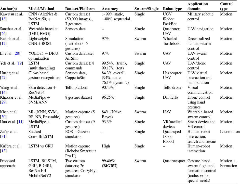
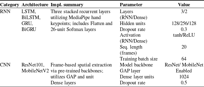

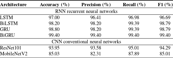

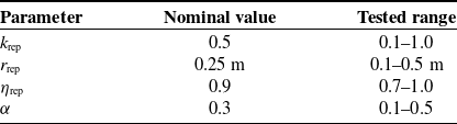

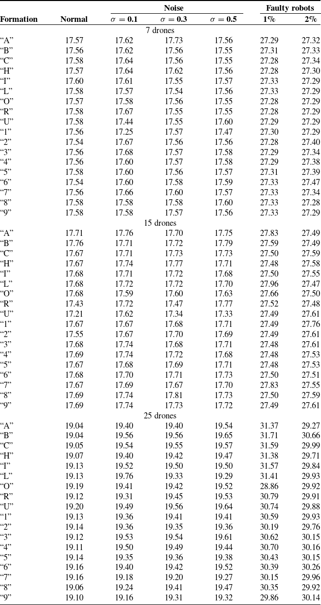
 σ
σ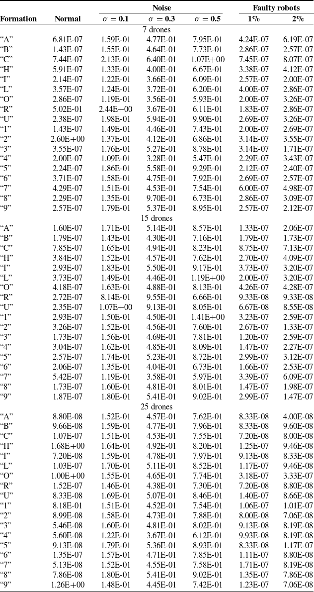
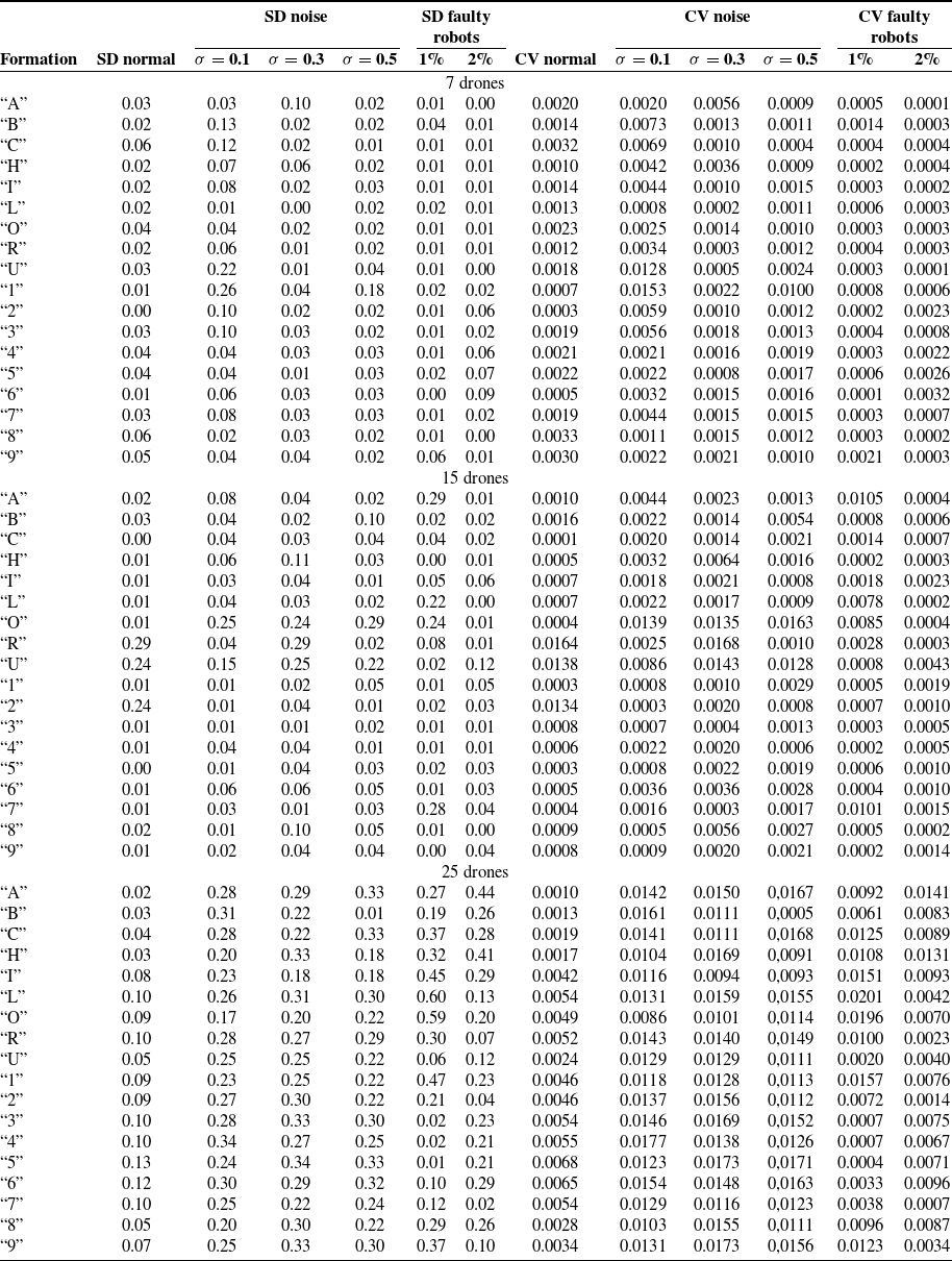
 σ
σ

 σ=0.1,0.3,0.5
 σ=0.1,0.3,0.5


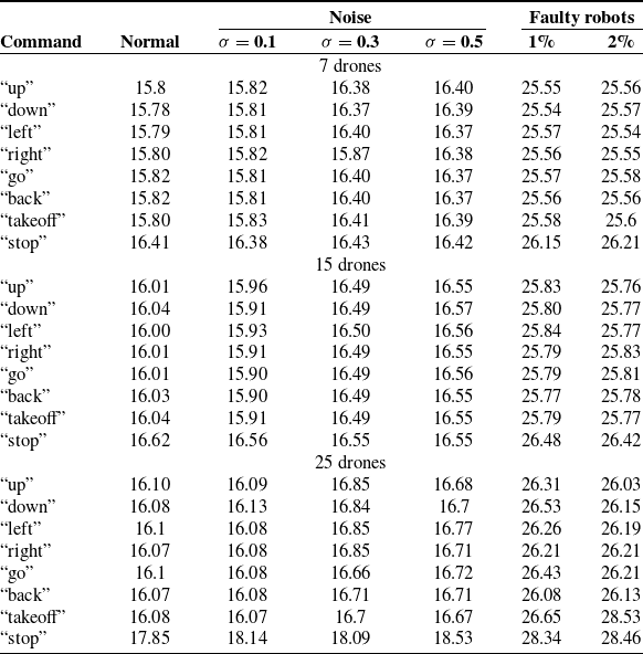
 σ
σ
 σ=0.1,0.3,0.5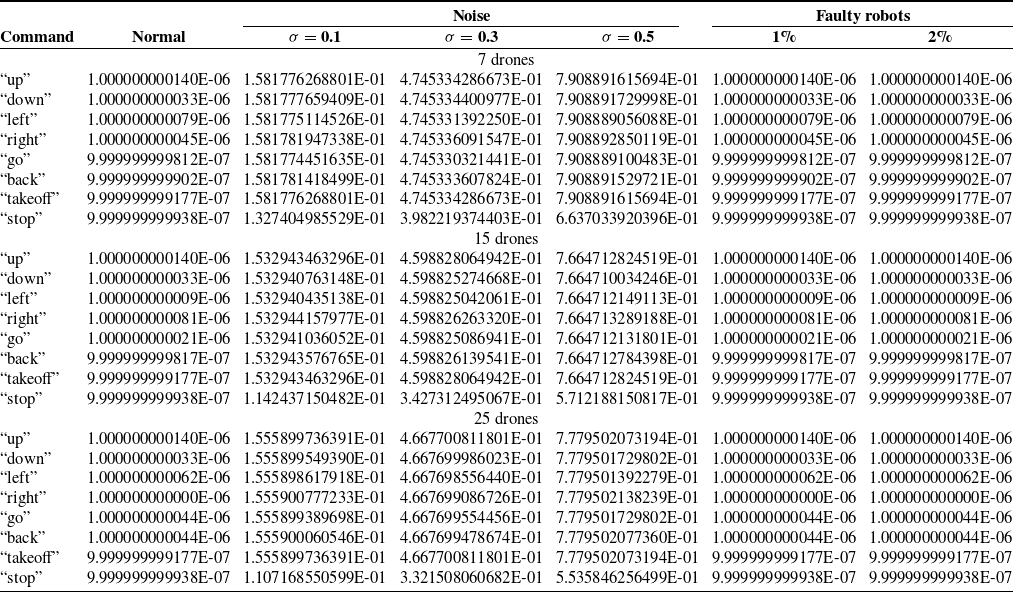
 σ
σ
 σ=0.1,0.3,0.5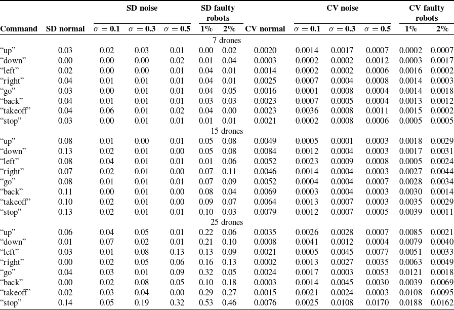
 σ
σ
 σ=0.1,0.3,0.5

 Open access

