2. The mathematical model

Our modelling framework consists of two partial differential equations (PDEs) describing the dynamics of biomass $B$ ( $\textrm{kg} \cdot \textrm{m}^2$ ) and toxicity $T$ ( $\textrm{kg} \cdot \textrm{m}^2$ ) within a smooth domain $\Omega \in \mathbb{R}^2$ . These variables are assumed to evolve as follows: biomass grows according to a growth rate $g$ inhibited by toxicity via a sensitivity coefficient $s$ , dies with a mortality rate $d$ and diffuses proportionally to the constant parameter $D_B$ . In particular, we assume that (even in the absence of toxicity) the biomass dynamics follows a logistic law, i.e. the biomass growth is limited by resource abundance via a carrying capacity term given by $g/d$ . On the other hand, toxicity increases proportionally to the biomass death via a coefficient $c$ , decays at rate $q$ , diffuses in the soil proportionally to $D_T$ and additionally spreads with a velocity $V_T$ in the downhill direction of the terrain whose slope is described by $m$ . The intensity of the total advection term is hence given by the product between these two quantities, which have been kept separate to emphasise their ecological derivation and to include an explicit space dependence linked with real topographical data in the future.

The above assumptions result in the following system of reaction-diffusion-advection equations:

(2.1a) \begin{align} \frac{\partial B}{\partial t} &= g\, B(1-s\,T)- d\,B^2 + D_B \, \Delta B, \end{align}

(2.1b) \begin{align} \frac{\partial T}{\partial t} &= c\, d\, B^2 - q\, T + D_T \, \Delta T + V_T \, m \, \partial _x T. \end{align}

A detailed description of the model parameters, together with their values and units, is illustrated in Table 1.

Table 1. Model parameters and their values for equations (2.1a), (2.1b)

3. Analysis

In order to investigate the emergence of patterned structures as well as travelling waves, we first reduce equations (2.1a), (2.1b) to a suitable nondimensional form. To this aim, we rescale the model variables as follows

(3.1) \begin{equation} \begin{gathered} \tilde{t} = g \, t, \quad \tilde{x} = \sqrt{\frac{g}{D_B}} x, \quad \tilde{y} = \sqrt{\frac{g}{D_B}} y \\[5pt] \tilde{B} = \frac{d}{g} B, \quad \tilde{T} = s \, T. \end{gathered} \end{equation}

Therefore, the corresponding nondimensional system is (we omit the tildes for the sake of readability)

(3.2a) \begin{align} \frac{\partial B}{\partial t} &= B(1-T)-B^2+ \Delta B, \end{align}

(3.2b) \begin{align} \frac{\partial T}{\partial t} &= \alpha B^2-\beta T + \gamma \, \partial _x T + \delta \Delta T, \end{align}

where we have introduced the following nondimensional parameters:

(3.3) \begin{equation} \alpha = \frac{c\, g\, s}{d}, \quad \beta =\frac{q}{g}, \quad \gamma =\frac{V_T \, m}{\sqrt{g\, D_B}}, \quad \delta = \frac{D_T}{D_B}. \end{equation}

The parameter $\alpha$ , representing the nondimensional production of $T$ due to $B$ , collects all the parameters contributing to the toxicity production; in particular, it describes the ratio between the biomass growth and death rates ( $g$ and $d$ , respectively) times the factors of conversion and sensitivity to toxicity ( $c$ and $s$ , respectively). Moreover, we note that the parameter $\beta$ here coincides with $\gamma$ in [Reference Cartenì, Marasco, Bonanomi, Mazzoleni, Rietkerk and Giannino8] – coherently with the structure for the $T$ equation presented here – and represents the characteristic rate of toxicity dynamics relative to plant growth rate. In particular, for fixed values of $g$ this parameter can be interpreted as the nondimensional version of the toxicity decay rate. The parameter $\gamma$ represents the ratio between the lateral flow of the toxicity and the radial diffusion of the biomass, whereas $\delta$ corresponds to the ratio between the two diffusion coefficients. According to the ranges identified for the dimensional parameters in Table 1, we have that

(3.4) \begin{equation} \alpha \in \left [0, 30\right ], \quad \beta \in \left [ \frac{1}{30}, \frac{1}{3} \right ], \quad \gamma \in \left [ 0, \sqrt{30} \right ], \quad \delta \in \left [ \frac 85, 4 \right ]. \end{equation}

3.1. Equilibria and stability

Equations (3.2a), (3.2b) admit two equilibria, obtained by solving

(3.5) \begin{equation} \begin{aligned} 0 &= B(1-T)-B^2, \\[5pt] 0 &= \alpha \, B^2-\beta \, T, \end{aligned} \end{equation}

and discarding the one which does not satisfy the feasibility assumption $B \geq 0$ . These two equilibria are

(3.6) \begin{equation} \begin{aligned} (B_0,T_0) &= (0,0) \quad &\text{(bare soil)},\\[5pt] (B_c,T_c) &= \left ( \frac{-\beta + \sqrt{\beta (4\alpha +\beta )}}{2 \alpha }, \frac{2\alpha + \beta -\sqrt{\beta (4\alpha +\beta )}}{2 \alpha } \right ) \quad &\text{(coexistence)}. \end{aligned} \end{equation}

The steady-state $(B_c,T_c)$ can also be written as $(\Gamma, 1-\Gamma )$ , with

(3.7) \begin{equation} \Gamma = \frac{-\beta + \sqrt{\beta (4\alpha +\beta )}}{2 \alpha }. \end{equation}

We note that the coexistence steady-state is monotonic in $\beta$ ; in particular, $B_c$ is increasing and $T_c$ is decreasing with respect to the parameter $\beta$ . This is consistent with the idea that the faster the toxicity is removed from the soil, the higher the biomass density and the lower the toxicity density, respectively. Conversely, $B_c$ is decreasing and $T_c$ is increasing with respect to the parameter $\alpha$ : as expected, in fact, higher values of the factors related to biomass which increase toxicity lead to higher toxicity and lower biomass at steady state (see Figure 1).

Figure 1. $B$ (left panel) and $T$ (right panel) components of the spatially homogeneous coexistence equilibria $(B_c, T_C)$ as functions of $\beta$ , for $\alpha =6$ (dotted line), $\alpha =18$ (dashed line) and $\alpha =30$ (solid line). $B_c$ is increasing in $\beta$ and decreasing in $\alpha$ , whereas $T_c$ is decreasing in $\beta$ and increasing in $\alpha$ .

Figure 2. Bifurcation diagram associated with equations (3.2a), (3.2b) with respect to parameter $\beta$ for $\alpha =18$ . The blue and purple lines correspond to $B_0$ and $B_c$ , respectively. Solid (resp. dashed) lines represent stability (resp. instability) with respect to spatially homogeneous perturbations, respectively.

3.1.1. Stability to homogeneous perturbations

The Jacobian matrix associated with equation (3.5) is given by

(3.8) \begin{equation} J= \begin{pmatrix} 1-2\,B_\ast -T_\ast\;\;\;\;\; & -B_\ast \\[5pt] 2 \, \alpha \, B_\ast\;\;\;\;\; & -\beta \end{pmatrix}, \end{equation}

where $(B_\ast, T_\ast )$ represents a generic equilibrium. We therefore have that (see also Figure 2)

• • The bare soil equilibrium is a saddle, since $J$ evaluated at $(B_0,T_0)$ admits the eigenvalues $\lambda _1=1,$ $\lambda _2=-\beta$ .

• • The coexistence equilibrium is stable, since $J$ evaluated at $(B_c,T_c)$ satisfies

  \begin{equation*} \begin {aligned} \textrm {tr}\,J \vert _{(B_c,T_c)} &= \frac {\beta (1-2 \alpha ) -\sqrt {\beta(4 \alpha +\beta )}}{2 \alpha } \lt 0, \\[5pt] \textrm {det}\,J \vert _{(B_c,T_c)} &= \frac {\beta \!\left (4 \alpha +\beta -\sqrt {\beta (4 \alpha +\beta )} \right )}{2 \alpha } \gt 0, \end {aligned} \end{equation*}
  for any $\alpha, \, \beta \gt 0$ .

3.1.2. Stability to heterogeneous perturbations

In order to investigate the stability of the steady-states (3.6) with respect to heterogeneous perturbations, we introduce the following non-uniform infinitesimal perturbations:

(3.9) \begin{equation} \begin{aligned} B(t,x,y) &= B_\ast + \tilde{B}(0)\, e^{i (k x+ l y)+\lambda t}, \\[5pt] T(t,x,y) &= T_\ast + \tilde{T}(0)\, e^{i (k x+ l y)+\lambda t}. \\[5pt] \end{aligned} \end{equation}

In particular, the norm of the spatial perturbation is defined as $h=\sqrt{k^2+l^2}$ .

When we linearise equations (3.2a), (3.2b) around the abovementioned steady states, we obtain the following system for the perturbations $\tilde{B}$ , $\tilde{T}$ (again we omit the tildes for sake of simplicity):

(3.10) \begin{equation} \begin{aligned} \lambda \, B &= (1-2\,B_\ast -T_\ast )\,B-B_\ast \,T-h^2 B, \\[5pt] \lambda \, T &= 2\, \alpha \,B_\ast \, B-\beta \, T+ i\, k\, \gamma \,T-\delta h^2\, T. \end{aligned} \end{equation}

Equation (3.10) is equivalent to an eigenvalue problem $J_h\, U = \lambda \, U$ , where $U=(B,T)$ and

(3.11) \begin{equation} J_h= \begin{pmatrix} 1-2\,B_\ast -T_\ast - h^2 & -B_\ast \\[5pt] 2 \, \alpha \, B_\ast & -\beta + i\, k\, \gamma -\delta \,h^2 \end{pmatrix}. \end{equation}

The characteristic polynomial, necessary to investigate the stability of (3.6), is given by

(3.12) \begin{equation} \lambda ^2-\textrm{tr}\,J_h \,\lambda +\textrm{det}\,J_h=0. \end{equation}

• • The eigenvalues of $J_h$ evaluated at $(B_0,T_0)$ are $\lambda _1=1-h^2$ , $\lambda _2=-\beta + i\, k\, \gamma -\delta \,h^2$ . Since this steady state is unstable with respect to homogeneous perturbations (see Section 3.1.1), no diffusion-driven instability occurs, and therefore, the stability character of the bare soil equilibrium is not relevant in the investigation of vegetation patterns. However, we observe that for $h$ such that $h^2\lt 1$ the bare soil equilibrium retains its saddle structure, whereas for $h$ such that $h^2\gt 1$ it becomes stable (hence diffusion may induce a stabilising effect, as often expected).

• • As for the coexistence equilibrium, we have that the trace and the determinant of $J_h$ evaluated at $(B_c,T_c)$ are

  (3.13) \begin{equation} \begin{aligned} \textrm{tr}\,J_h &= -\beta -\Gamma -h^2(\delta +1)+ i\,k\,\gamma, \\[5pt] \textrm{det}\,J_h &= (h^2+\Gamma )(\beta +\delta \, h^2-i\,k\,\gamma )+2\,\alpha \,\Gamma ^2. \end{aligned} \end{equation}
  Equation (3.12) is solved by two roots given by
  (3.14) \begin{equation} \lambda _\pm =\frac 12 \left ( -\beta -\Gamma -h^2(\delta +1)+i\,k\,\gamma \right ) \pm \sqrt{X+i\,Y}, \end{equation}
  where
  (3.15) \begin{equation} \begin{aligned} X &= (\beta - \Gamma +h^2(\delta -1))^2 - k^2\,\gamma ^2-8\,\alpha \,\Gamma ^2, \\[5pt] Y &= -2\,k\,\gamma \left ( \beta -\Gamma +h^2(\delta -1) \right ). \end{aligned} \end{equation}
  The real and imaginary part of the eigenvalues (3.14) can be written as
  (3.16a) \begin{align} \textrm{Re}\,\lambda &= \frac 12 \left ( -\beta -\Gamma -h^2(\delta +1)+j\sqrt{\frac{X+\sqrt{X^2+Y^2}}{2}} \right ), \end{align}
  (3.16b) \begin{align} \textrm{Im}\,\lambda &= \frac 12 \left ( \,k\,\gamma +j\, \textrm{sgn}(Y) \sqrt{\frac{\sqrt{X^2+Y^2}-X}{2}} \right ), \end{align}

  where $j=\pm 1$ . In order for patterns to emerge, there must exist $k$ , $l$ such that $\textrm{Re}\,\lambda \gt 0$ [Reference Murray30]. It is already clear that this condition cannot be satisfied in the case $j=-1$ ; therefore, we focus our forthcoming analysis on the case $j=+1$ . Since the right-hand side of (3.16a) is given by the sum of a positive term (the square root) and a negative term (the rest), for this quantity to be positive it must be

  \begin{equation*} \sqrt {\frac {X+\sqrt {X^2+Y^2}}{2}} \gt \beta +\Gamma +h^2(\delta +1). \end{equation*}
  Using the ranges determined for the nondimensional parameters in (3.4), we have that $\textrm{Re}\,\lambda \lt 0$ for any $h$ and for any $\alpha$ , $\beta$ , $\delta$ in (3.4). Therefore, no Turing patterns can emerge.

3.2. Travelling waves

In this section, we consider the formation of travelling wave profiles, i.e. profiles which move through the spatial domain keeping constant shape and speed.

Extensive simulations of equations (2.1a), (2.1b) reveal that one-dimensional sections of compact initial data $B(0,x,y)$ and $T(0,x,y)$ numerically evolve into travelling waves for a wide parameter range (see Figure 3, Section 4). In particular, the unstable nature of the trivial steady-state $(B_0, T_0)$ suggests we are in the presence of pulled fronts, where the linear spreading of small perturbations pulls the front into the linearly unstable bare soil steady-state [Reference Lewis, Li and Weinberger22, Reference Maini, McElwain and Leavesley24, Reference van Saarloos39]. The (nondimensional) asymptotic travelling speed of such structures $\tilde{c}_\infty$ therefore coincides with the linear spreading speed $\tilde{c}_\infty$ . In order to compute it, we introduce the characteristic polynomial of the Jacobian matrix associated with equations (3.2a), (3.2b) evaluated at $(B_0,T_0)$ focusing on one-dimensional domains:

(3.17) \begin{equation} p_0(\lambda ) \;:\!=\; \lambda ^2+ \mathcal{A}_1 \, \lambda + \mathcal{A}_0, \end{equation}

where

(3.18) \begin{equation} \begin{aligned} \mathcal{A}_1 &\;:\!=\; k \, (k \, (1+\delta ) - i \, \gamma ) + \beta -1, \\[5pt] \mathcal{A}_0 &\;:\!=\; \left ( k^2-1 \right ) \left ( k \, (\delta \, k - i \, \gamma )+\beta \right ). \end{aligned} \end{equation}

The dispersion relation, corresponding to the solution to $p_0(\lambda )=0$ with the largest real part, is given by

(3.19) \begin{equation} \lambda (k) = 1-k^2. \end{equation}

The linear spreading speed $\tilde{c}_\infty$ is obtained by solving (see [Reference Murray30])

(3.20a) \begin{align} i \, \tilde{c}_\infty + \lambda '(k_0) &= 0, \end{align}

(3.20b) \begin{align} \textrm{Re} \left [ i \, \tilde{c}_\infty \, k_0 + \lambda (k_0) \right ] &= 0. \end{align}

Here, $k_0$ is a constant related to the asymptotic evaluation of the Fourier transform of the perturbation solving the linearised system via the method of steepest descents for $t \to \infty$ . Equation (3.20b), on the other hand, represents the assumption that such perturbation neither grows nor decays at the leading edge of the front.

Figure 3. Travelling arc moving uphill obtained by numerically simulating equations (2.1a), (2.1b) at four different time steps for biomass ( $B$ ), toxicity ( $T$ ) (first and second row panels) and a one-dimensional cross-section obtained by cutting the profiles in the middle of the two-dimensional domain along the direction of the slope. The parameter values used for the simulation are taken from Table 1 together with $m=0.5$ , $q=0.01$ , $s=3$ , $D_T=1.2$ , and $V_T=5$ .

Since $\tilde{c}_\infty \in \mathbb{R}$ , equation (3.20a) implies $k_0 = \dfrac{i \, \tilde{c}_\infty }{2}$ . Plugging this into equation (3.20b) (and focusing our attention on right-moving fronts, i.e. fronts with positive speed), we obtain

(3.21) \begin{equation} \tilde{c}_\infty = 2. \end{equation}

(This, in turn, leads to $k_0=i$ ). We note that this coincides with the critical wave speed of a travelling wave solution to the Fisher-KPP equation (see e.g. [Reference Murray31]). Heuristically, this can be explained by the absence of toxicity at the leading edge of the front, which turns equation (3.2a) precisely into the Fisher-KPP equation.

In order to compare this result with numerical simulations of the dimensional model (2.1a), (2.1b) and to facilitate the ecological interpretation of this quantity, we convert $\tilde{c}_\infty$ into its dimensional version $c_\infty$ by recalling that, due to equation (3.1), we have $\frac{dx}{dt} = \sqrt{D_B \, g} \, \frac{d\tilde{x}}{d\tilde{t}}$ , therefore

(3.22) \begin{equation} c_\infty = 2\sqrt{D_B \, g}. \end{equation}

The right-moving front hence moves with constant shape and speed $\tilde{c}_\infty$ , which solely depends on the biomass growth rate and its diffusion coefficient. The presence of the slope, regulated by the parameter $\gamma$ , induces the formation of a travelling arc (in the uphill direction) for $\gamma \gt 0$ (see Figure 3), i.e. the ‘tail’ of the ring is disrupted by the downhill flow of toxicity. Turning off the effect induced by toxicity via the slope term by considering $\gamma =0$ –representing a flat ground – substantially changes the structure of the emerging pattern: the travelling arc reduces to a ring symmetrically expanding in all directions and, depending on the intensity of the toxicity parameters, secondary travelling rings may form inside the primary ring (see Figure 4). In both cases, we recall that the stability analysis illustrated in Section 3.1.2 implies that, as $t \to \infty$ , we have convergence to the uniform equilibrium $(B_c,T_c)$ .

Figure 4. Travelling ring obtained by numerically simulating equations (2.1a), (2.1b) at four different time steps for biomass ( $B$ ), toxicity ( $T$ ) (first and second row panels) and a one-dimensional cross-section obtained by cutting the profiles in the middle of the symmetric two-dimensional domain. The parameter values used for the simulation are taken from Table 1 together with $m=0$ , $q=0.01$ , $s=3$ , and $D_T=1.2$ .

4. Numerical simulations

In this section, we perform a series of numerical simulations of equations (2.1a), (2.1b) equipped with Neumann boundary conditions on a two-dimensional square domain $[0, L] \times [0, L]$ using the software Matlab. As for the initial conditions, we set

(4.1) \begin{equation} B(0,x,y) =B_i(x,y), \qquad T(0,x,y) =T_i(x,y) \end{equation}

where $B_i(x,y) = 0$ everywhere except for $B_i(L/2,L/2)=0.5$ ( $\textrm{kg} \cdot{m}^{-2}$ ) and $T_i(x,y)=0$ ( $\textrm{kg} \cdot{m}^{-2}$ ) for all $x, y$ . We note that from here on we focus on the dimensional model, as dimensional parameters and quantities are easier to interpret from the ecological viewpoint.

In Figure 5, we investigate the influence of toxicity on the structure of the emerging travelling patterns by comparing the simulated one-dimensional profiles in the cases $s \gt 0$ (biomass dynamics affected by toxicity) and $s=0$ (biomass and toxicity dynamics decoupled) on a sloped terrain at a fixed instant. We observe that, while in the first case a travelling pulse arises moving in the uphill direction, in the second case this pulse reduces to two fronts symmetrically travelling in an outward direction. The maximum peak reached by the biomass is also sensibly lower in the case $s\gt 0$ ; toxicity further influences this quantity via the slope parameter $m$ , as investigated below (see Figure 6).

Figure 5. Comparison between two one-dimensional cross sections of biomass profiles obtained by simulating equations (2.1a), (2.1b) with initial conditions as in (4.1) for $D_B=0.5$ , $g=0.6$ , $d=0.06$ , $c=0.6$ , $V=5$ , $D_T=1.2$ , $q=0.01$ , $m=0.5$ and $s=3$ (solid line) vs $s=0$ (dashed line). In the first case, a travelling pulse forms which moves along the slope direction, whereas in the second case, we have two travelling fronts symmetrically moving outwards.

Figure 6. Variations in the peak of biomass ( $B$ , left vertical axis, continuous line) and toxicity ( $T$ , right vertical axis, dashed line) due to changes in slope ( $m$ ). The parameter values used for the simulation are taken from Table 1 with $k=0.01$ , $s=3$ , $D_T=1.2$ , and $V_T=5$ .

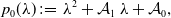
Figure 7. Analytical representation (equation (3.22), continuous line) and numerical simulations (circles) of the asymptotic travelling speed $c_\infty$ with respect to the biomass growth parameter $g$ (left panel) and the biomass diffusion parameter $D_B$ (right panel). The other parameter values used for the simulation are taken from Table 1 together with $m=0.5$ , $k=0.01$ , $s=3$ , $D_T=1.2$ and $V_T=5$ .

The next step in our numerical investigation focuses on the influence of the toxicity on the arising travelling patterns via the slope parameter $m$ . First, we analyse the scenario of a sloped terrain represented by $m\gt 0$ in Figure 3, which shows the evolution of the system’s dynamics at increasing time steps corresponding to 10, 50, 100 and 150 months. In this simulation, the slope coefficient $m$ is set to $0.5$ , with the uphill direction corresponding to the right-hand side of the domain. The first two rows represent the accumulation of biomass and toxicity in the square grid, respectively. As expected, biomass starts growing radially until it is inhibited by the presence of toxicity which, due to the advection term in equations (2.1a), (2.1b), diffuses prominently in the downhill direction. This induces the emergence of a travelling arced shape of biomass. This behaviour is displayed also in the third row of Figure 3 via a one-dimensional horizontal section of the square numerical domain showing the evolution in time of both biomass and toxicity.

An analogous temporal evolution of the system’s dynamics in the case of flat grounds (represented by the case $m=0$ ) is shown in Figure 4. Here, the radial growth of the biomass is symmetrically affected by toxicity and hence not disrupted, leading to rings expanding in the two-dimensional domain. With the parameter values adopted in this simulation, secondary rings form within the primary ring as a result of the fact that, after some time, the toxicity removed from the centre of the domain creates the conditions for new biomass growth. This result is consistent with the findings presented in [Reference Cartenì, Marasco, Bonanomi, Mazzoleni, Rietkerk and Giannino8].

Due to the importance of the slope intensity in the toxicity advection term, we evaluate numerically the dependence between the slope parameter $m$ and the height of the leading travelling pulse both for biomass and toxicity. As expected by the mathematical formulation, the higher the slope, the higher the advection which reduces, even if only slightly, the toxicity and its maximum peak (Figure 6). This decrease in the toxicity then induces a corresponding increase in the biomass peak of the main travelling pulse.

Finally, as the asymptotic travelling speed $c_\infty$ was shown to depend only on $D_B$ and $g$ (see equation (3.22)), we compare this expression with the numerically calculated velocity by varying both of these parameters. The numerical speed was calculated as the ratio of the number of pixels covered by the travelling peak to the number of timesteps (converted to m/month) with parameter values as in Table 1 and $k=0.01$ , $s=3$ , $D_T=1.2$ , $V_T=5$ . In both cases, numerical results are in good agreement with the analytical predictions (see Figure 7).