


1. Introduction
Rotating thermal convection (Ecke & Shishkina Reference Ecke and Shishkina2023) is a widespread phenomenon observed in the fluid cores of stars and planets, planetary atmospheres, terrestrial oceans and industrial processes (Greenspan Reference Greenspan1968; Busse & Carrigan Reference Busse and Carrigan1976; Kunnen Reference Kunnen2021). Investigations of rotating thermal convection in astrophysical and geophysical flows are of immense significance in comprehending the mechanisms of heat and momentum transport, as well as the maintenance of the magnetic field in the many planets and stars such as the Earth and Sun (Aurnou et al. Reference Aurnou, Calkins, Cheng, Julien, King, Nieves, Soderlund and Stellmach2015; Hanasoge, Gizon & Sreenivasan Reference Hanasoge, Gizon and Sreenivasan2016; Yadav et al. Reference Yadav, Gastine, Christensen, Duarte and Reiners2016; Schumacher & Sreenivasan Reference Schumacher and Sreenivasan2020; Yadav & Bloxham Reference Yadav and Bloxham2020). Rotating Rayleigh–Bénard convection (RRBC) has been served as a canonical model to examine rotation-influenced buoyancy-driven flows for decades (Chandrasekhar Reference Chandrasekhar1953; Rossby Reference Rossby1969; Ecke & Shishkina Reference Ecke and Shishkina2023). In this model system the fluid is heated from below and cooled from above (with the temperature difference,  $\varDelta$) and confined between two parallel horizontal plates separated by a distance of $L$. The system rotates with a constant angular velocity $\varOmega$ in the vertical direction. Studies of RRBC have been focused on (1) the effects of rotation on heat transfer modifications and flow structures as compared with its non-rotating counterpart; (2) the role of the Ekman boundary layer (BL) and resulting Ekman pumping in controlling heat transfer; (3) the dynamics and formation of large-scale vortices induced by the inverse energy cascade; (4) the geostrophic flow regime at very low $Ek$ and high $Ra$ (defined below); (5) the boundary zonal flow that occurs near the lateral sidewall and its relation to the wall modes; and (6) other effects such as the non-Oberbeck–Boussinesq effects. For more general introduction on RRBC with these topics, we refer to the reviews by Kunnen (Reference Kunnen2021) and Ecke & Shishkina (Reference Ecke and Shishkina2023).
One of the most important tasks in RRBC studies is to comprehend the scaling relations between the system's global response and the control parameters (Kunnen Reference Kunnen2021; Ecke & Shishkina Reference Ecke and Shishkina2023). The three control parameters are the Rayleigh number  $Ra$, which is the dimensionless temperature difference between the two plates, the Prandtl number $Pr$, which represents the fluid's diffusive properties, and the Ekman number $Ek$, which is the ratio of viscous force to Coriolis force or, alternatively, the convective Rossby number $Ro_c$, which denotes the ratio of buoyancy to rotation strength. They are defined as
 \begin{equation} Ra=\frac{\alpha_T g L^3 \varDelta }{\kappa \nu}, \quad Pr=\frac{\nu}{\kappa},\quad Ek=\frac{\nu}{2\varOmega L^2},\quad Ro_c=\frac{\sqrt{\alpha_T g\varDelta/L}}{2\varOmega}. \end{equation}
Here,  $\nu$, $\kappa$ and $\alpha _T$ are the kinematic viscosity, thermal diffusivity and thermal expansion coefficient of the fluid, respectively. The system's responses are mainly quantified by the dimensionless heat transport represented by the Nusselt number $Nu$ and the momentum transport denoted by the Reynolds number $Re$, as
 \begin{equation} Nu = \frac{\langle u_z \theta \rangle-\kappa \partial_z \langle\theta\rangle}{\kappa \varDelta / L},\quad Re = \frac{uL}{\nu}. \end{equation}
Here,  $u$ is the typical velocity, $u_z$ the vertical component of the velocity, $\theta$ the temperature and $\langle \cdots \rangle$ denotes averaging in time and over any horizontal cross-section. The scaling relations of $Nu$ and $Re$ are sought in the form $\sim Ra^{\alpha }Ek^{\beta }Pr^{\gamma }$. Numerous studies have been conducted to study the heat transfer scaling relations in RRBC (e.g. see the reviews by Plumley & Julien Reference Plumley and Julien2019; Kunnen Reference Kunnen2021; Ecke & Shishkina Reference Ecke and Shishkina2023).
Under strong rotation ( $Ek\leq 10^{-4}$), with increasing thermal driving strength $Ra$, RRBC undergoes transitions among distinct flow regimes: the onset of convection, rotation-dominated, rotation-affected and buoyancy-dominated convection (Cheng et al. Reference Cheng, Aurnou, Julien and Kunnen2018; Kunnen Reference Kunnen2021; Ecke & Shishkina Reference Ecke and Shishkina2023). Close to the onset of steady convection, the critical value of $Ra_c$ for instability scales as $Ra_c\approx 8.7Ek^{-4/3}$, and the typical convective length scales as $\ell /L \approx 2.4Ek^{1/3}$ for $Pr\geq 0.68$ (Chandrasekhar Reference Chandrasekhar1953, Reference Chandrasekhar1961). In the rotation-dominated regime the primary balance of forces is between the Coriolis force and the pressure gradient terms, which is also known as the geostrophic balance (Greenspan Reference Greenspan1968). For moderate supercriticality $RaEk^{4/3}$, which is proportional to $Ra/Ra_c$, the heat transport follows the scaling law $Nu\sim (RaEk^{4/3})^{\alpha }$ for a certain positive $\alpha$, and the flow consists of coherent, vertically aligned columns or plumes that transport cold and hot fluid downward and upward, respectively (Julien et al. Reference Julien, Knobloch, Rubio and Vasil2012a; Nieves, Rubio & Julien Reference Nieves, Rubio and Julien2014; Stellmach et al. Reference Stellmach, Lischper, Julien, Vasil, Cheng, Ribeiro, King and Aurnou2014; Cheng et al. Reference Cheng, Stellmach, Ribeiro, Grannan, King and Aurnou2015; Kunnen Reference Kunnen2021). Using the marginal thermal BL instability criterion, Boubnov & Golitsyn (Reference Boubnov and Golitsyn1990) theoretically derived the scaling law $Nu\sim Ra^{3}Ek^{4}$ for the rotation-dominated regime; see also King, Stellmach & Aurnou (Reference King, Stellmach and Aurnou2012). This steep scaling law has been observed in direct numerical simulations (DNS) and experiments of planar RRBC with no-slip boundary conditions for $Ek\geq 10^{-6}$ (King et al. Reference King, Stellmach and Aurnou2012; Stellmach et al. Reference Stellmach, Lischper, Julien, Vasil, Cheng, Ribeiro, King and Aurnou2014). Moreover, experiments show a trend of ever-steepening scaling with the exponent $\alpha \approx 3.6$ as $Ek$ further decreases to $Ek\approx 3\times 10^{-8}$ at $Pr=7$ (Cheng et al. Reference Cheng, Stellmach, Ribeiro, Grannan, King and Aurnou2015). For a chaotic flow where the viscous effects are not negligible, the so-called viscous–Archimedean–Coriolis (VAC) force balance gives rise to the momentum transport scaling of $Re\sim Ra^{1/2}(Nu-1)^{1/2}Ek^{1/3}Pr^{-1}$ (Gillet & Jones Reference Gillet and Jones2006; Aurnou, Horn & Julien Reference Aurnou, Horn and Julien2020; Hawkins et al. Reference Hawkins, Cheng, Abbate, Pilegard, Stellmach, Julien and Aurnou2023; Madonia et al. Reference Madonia, Guzmán, Clercx and Kunnen2023).
Using asymptotically reduced equations (Sprague et al. Reference Sprague, Julien, Knobloch and Werne2006), for the rotationally constrained regime with  $Ek\rightarrow 0$, an inviscid heat transfer scaling of $Nu\sim Ra^{3/2}Ek^{2}Pr^{-1/2}$ was derived by Julien et al. (Reference Julien, Knobloch, Rubio and Vasil2012a). This regime of the geostrophic turbulence can also be derived from the Coriolis, inertia and Archimedean (CIA) force balance or from the inviscid theory (Stevenson Reference Stevenson1979; Gillet & Jones Reference Gillet and Jones2006; Guervilly, Cardin & Schaeffer Reference Guervilly, Cardin and Schaeffer2019; Aurnou et al. Reference Aurnou, Horn and Julien2020). The corresponding diffusion-free momentum and convective length scales are $Re\sim RaEkPr^{-1}$ and $\ell /L\sim (ReEk)^{1/2}= Ro^{1/2}=Ra^{1/2}EkPr^{-1/2}$, respectively, as shown by Guervilly et al. (Reference Guervilly, Cardin and Schaeffer2019), Aurnou et al. (Reference Aurnou, Horn and Julien2020), Madonia et al. (Reference Madonia, Guzmán, Clercx and Kunnen2023) and Hawkins et al. (Reference Hawkins, Cheng, Abbate, Pilegard, Stellmach, Julien and Aurnou2023). Here the Rossby number is defined as $Ro=u/(2\varOmega L)$. Remarkably, the diffusion-free heat transfer scaling of $Nu\sim Ra^{3/2}Ek^{2}Pr^{-1/2}$ is analogous to the ultimate regime in non-rotating RB, where the heat transport is independent of diffusion and the flow is bulk-dominated (Ahlers, Grossmann & Lohse Reference Ahlers, Grossmann and Lohse2009; Lohse & Xia Reference Lohse and Xia2010). This scaling has been observed in DNS of RRBC in planar configuration with stress-free boundary conditions and asymptotically reduced models without Ekman pumping (Julien et al. Reference Julien, Knobloch, Rubio and Vasil2012a; Stellmach et al. Reference Stellmach, Lischper, Julien, Vasil, Cheng, Ribeiro, King and Aurnou2014; Plumley et al. Reference Plumley, Julien, Marti and Stellmach2017). Recently, Bouillauta et al. (Reference Bouillauta, Miquela, Julien, Aumaître and Gallet2021) observed such heat transport scaling in an experimental set-up where convection is driven radiatively. The ultimate heat transport scaling was verified via DNS for a no-slip insulating bottom boundary and a stress-free insulating top one. Previously, the diffusion-free heat transport was observed in spherical RB convection with no-slip boundary conditions and $Ek\leq 10^{-5}$ (Gastine, Wicht & Aubert Reference Gastine, Wicht and Aubert2016; Wang et al. Reference Wang, Santelli, Lohse, Verzicco and Stevens2021), where it arises from the complex interplay of convection dynamics in polar and equatorial regions (Gastine & Aurnou Reference Gastine and Aurnou2023). Not only the diffusion-free convective heat, but also the diffusion-free momentum and length scale of the geostrophic turbulence regime have been elucidated theoretically and verified in DNS of RRBC in planar geometry with no-slip boundary conditions at extreme buoyancy and rotation parameters (up to $Ra =3 \times 10^{13}$ and down to $Ek=5\times 10^{-9}$) (Song, Shishkina & Zhu Reference Song, Shishkina and Zhu2024). A primary objective of this study is to further broaden the parameter range, allowing us to investigate both the CIA balance regime and the VAC balance regime and to illustrate the gradual transition between these two regimes.
Beyond the rotation-dominated regime, there is a rotation-affected regime, where the Coriolis force is important but not dominant; this regime is characterized by the emission of vertical thermal plumes from the BL and the absence of large-scale vortices (Cheng et al. Reference Cheng, Aurnou, Julien and Kunnen2018, Reference Cheng, Madonia, Guzmán and Kunnen2020; Ecke & Shishkina Reference Ecke and Shishkina2023). Recently, Cheng et al. (Reference Cheng, Madonia, Guzmán and Kunnen2020) conducted experiments using the TROCONVEX facility with water at  $Pr\approx 5.2$ and very high $Ra\sim 10^{13}$ and low $Ek\sim 10^{-8}$, and identified a turbulence regime influenced by rotation where $Nu\sim Ra^{0.52}$. They suggested that this intermediate regime of rotation-affected convection becomes wider as $Ek$ decreases. The heat transport enhancement in the rotation-affected regime with $Pr\geq 4.38$ has been investigated by Yang et al. (Reference Yang, Verzicco, Lohse and Stevens2020) and Hartmann et al. (Reference Hartmann, Yerragolam, Verzicco, Lohse and Stevens2023). For relatively low $Ra\lesssim 5\times 10^{8}$, they found that the optimal heat transport enhancement occurs when the thicknesses of the viscous and thermal BL are approximately equal; while for high $Ra\gtrsim 5\times 10^{8}$, the heat transport enhancement becomes smaller as the bulk flow at these values of $Ra$ in the rotation-affected regime changes to geostrophic turbulence. As $Ra$ further increases, the flow enters the buoyancy-dominated regime, where the effect of the Coriolis force becomes negligible. In this regime, the flow structures and scaling relations approach those observed in non-rotating RB convection (Ahlers et al. Reference Ahlers, Grossmann and Lohse2009; Ecke & Shishkina Reference Ecke and Shishkina2023).
As described above, RRBC exhibits several distinct flow regimes, each with its own heat transport scaling relation. Also very recently, both the VAC- and CIA-based  $Re$ scaling relations are shown to be applicable to different flow regimes of some experimental and DNS datasets (Hawkins et al. Reference Hawkins, Cheng, Abbate, Pilegard, Stellmach, Julien and Aurnou2023; Madonia et al. Reference Madonia, Guzmán, Clercx and Kunnen2023). To verify and assess these scaling relations in different flow regimes, we have conducted extensive DNS of RRBC in planar geometry, across a wide range of parameters, including nine Ekman numbers spanning $5\times 10^{-9}\leq Ek \leq 5\times 10^{-5}$, Rayleigh numbers within the range $5\times 10^{6}\leq Ra \leq 5\times 10^{13}$ and a unity Prandtl number. To the authors’ knowledge, $Ra=5\times 10^{13}$ is the most extreme $Ra$ achieved so far in DNS for RRBC. The DNS has revealed not only the typical flow regimes of rotation-dominated flow, namely, cellular flow, Taylor columns, plumes, geostrophic turbulence and large-scale vortices, but also the buoyancy-dominated flow. The typical flow structures for rotation-dominated regimes and turbulent statistics associated with viscous and thermal BLs of all these flow regimes are studied in detail. Importantly, the scaling relations for $Nu$, the global and local $Re$, the convective length as well as the temperature drop within the thermal BL and its thickness are examined for these flow regimes, which further indicate the achievement of the diffusion-free regime of geostrophic turbulence at extreme parameters (very small $Ek\leq 1.5\times 10^{-8}$ and very large $Ra\geq 10^{13}$) in the present study. Furthermore, our investigation reveals a clear transition from the VAC- to CIA-balanced momentum transport scaling behaviour with increasing $Ra$ and decreasing $Ek$.
$Ek$.
The paper is organised as follows. In § 2 we introduce the numerical models and governing equations and describe the computational details. Flow structures and typical turbulent statistics associated with viscous and thermal BLs are shown in § 3. Scaling behaviours of the heat, momentum transport and convective length scale are discussed in § 4. We give our conclusions in § 5.
2. Problem formulation and computational details
The Boussinesq approximation is used to describe RRBC of a fluid between two horizontal plates, which is rotated with a constant angular velocity  $\varOmega$ around the vertical axis $z$, under gravitational acceleration $g=-g\boldsymbol {e}_z$, where $\boldsymbol {e}_z$ is the vertical unit vector. The chosen reference scales are the height of the domain $L$, the temperature difference between the plates $\varDelta$ and the characteristic free-fall velocity $U_{ff}=\sqrt {g\alpha _T\Delta L}$. Non-dimensional temperature $\theta$, velocity $\boldsymbol {u}$, pressure $p$ and time $t$ are obtained using these scales. The dimensionless governing equations for the incompressible fluid are
 $$\begin{gather} \boldsymbol{\nabla}\boldsymbol{\cdot}\boldsymbol{u} = 0, \end{gather}$$
 $$\begin{gather}\frac{\partial \boldsymbol{u}}{\partial t}+\boldsymbol{u}\boldsymbol{\cdot}\boldsymbol{\nabla}\boldsymbol{u} ={-}\boldsymbol{\nabla} p+\sqrt{\frac{Pr}{Ra}}\nabla^2\boldsymbol{u}+\theta\boldsymbol{e}_z -\frac{1}{Ek}\sqrt{\frac{Pr}{Ra}}\boldsymbol{e}_z\times\boldsymbol{u}, \end{gather}$$
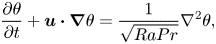 $$\begin{gather}\frac{\partial \theta}{\partial t} + \boldsymbol{u}\boldsymbol{\cdot}\boldsymbol{\nabla} \theta = \frac{1}{\sqrt{RaPr}}\nabla^2\theta, \end{gather}$$
and all results in this paper will be presented in the dimensionless form. No-slip boundaries and constant temperature conditions at the bottom and top plates, as well as periodic boundary conditions in both horizontal directions were applied. We consider periodic boundary conditions in the lateral directions, in order to avoid the influence of the wall modes that develop next to the sidewalls in rapidly RRBC (Ecke, Zhong & Knobloch Reference Ecke, Zhong and Knobloch1992; Herrmann & Busse Reference Herrmann and Busse1993; Favier & Knobloch Reference Favier and Knobloch2020; Shishkina Reference Shishkina2020; Zhang et al. Reference Zhang, van Gils, Horn, Wedi, Zwirner, Ahlers, Ecke, Weiss, Bodenschatz and Shishkina2020; Zhang, Ecke & Shishkina Reference Zhang, Ecke and Shishkina2021; Ecke, Zhang & Shishkina Reference Ecke, Zhang and Shishkina2022). The centrifugal buoyancy is not considered due to its weak role in the flow of the planetary core convection. To solve the governing equations, an energy-conserving second-order finite-difference code AFiD was utilized (Verzicco & Orlandi Reference Verzicco and Orlandi1996; van der Poel et al. Reference van der Poel, Ostilla-Mónico, Donners and Verzicco2015; Zhu et al. Reference Zhu2018). The original code was updated to include a Coriolis force term in the momentum equations to account for system rotation. The code was parallelized using a two-dimensional pencil domain decomposition strategy, allowing it to effectively handle large-scale computations (van der Poel et al. Reference van der Poel, Ostilla-Mónico, Donners and Verzicco2015). To ensure a proper resolution of the flow and temperature fields, sufficiently large computational domains and grid mesh sizes were used for each studied case. Specifically, in every studied case, the computational domain size is large enough to capture the typical flow structures: the horizontal extension of the domain is at least  $20$ times larger than the onset convective length scale of $2.4Ek^{1/3}$ (Chandrasekhar Reference Chandrasekhar1961). A Chebyshev-like distribution of the grid points is applied in the wall normal $z$ direction and a uniform distribution in the periodic $x$ and $y$ directions, so that the grid points are clustered near the bottom and top plates. A proper grid resolution is needed within the BLs, especially for the thin viscous (Ekman) BL, which requires special attention (Stellmach et al. Reference Stellmach, Lischper, Julien, Vasil, Cheng, Ribeiro, King and Aurnou2014; Aguirre Guzmán et al. Reference Aguirre Guzmán, Madonia, Cheng, Ostilla-Mónico, Clercx and Kunnen2021; Hartmann et al. Reference Hartmann, Yerragolam, Verzicco, Lohse and Stevens2023). In our simulations, there are always at least $10$ grid points in each thermal and viscous (Ekman) BL. In order to check the bulk grid resolution used in the DNS, we calculated the mean dimensionless Kolmogorov microscale (normalised by $L$)
$L$)  $\eta \equiv \nu ^{3/4}\langle \epsilon _u\rangle _V^{-1/4}$, where $\langle \epsilon _u\rangle _V$ denotes the volume and temporal averaged kinetic energy dissipation rate. The maximum values of the ratio of the mesh size to the mean Kolmogorov microscale are listed in table 1 in the Appendix. The maximal value of the ratio of the mesh size to the mean Kolmogorov microscale, even for the highest $Ra = 5.0 \times 10^{13}$, is always smaller than 2.5; this value was empirically found to be acceptable (Verzicco & Camussi Reference Verzicco and Camussi2003; Shishkina et al. Reference Shishkina, Stevens, Grossmann and Lohse2010; Scheel, Emran & Schumacher Reference Scheel, Emran and Schumacher2013). Sufficiently long preliminary simulations (at least $400$ free-fall time units) were performed to ensure statistically steady flow states are achieved. After that, ensemble averages are obtained over a time period of $\geq$200 free-fall time units (see table 1 in the Appendix for details of the averaging interval). The convergence of the Nusselt numbers are checked for the entire domain and the BL flow scales are well resolved. In this study the maximum relative errors of the Nusselt numbers calculated by five different methods listed in the Appendix were less than
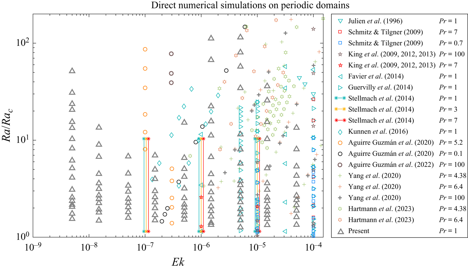
  $1\,\%$ (see the Appendix for computational details). The explored parameter range of DNS on RRBC with periodic boundary conditions on the lateral directions are summarised in figure 1. It should be noted that in combination with Song et al. (Reference Song, Shishkina and Zhu2024), our extensive DNS has extended the one and half-decade old previously explored $Ek$ parameter range.
Phase diagram of DNS on RRBC with periodic lateral boundary conditions for different  $Ek$ and $Ra/Ra_c$, where $Ra_c$ is the critical value for the onset instability (Chandrasekhar Reference Chandrasekhar1953; Kunnen Reference Kunnen2021). The data comes from Julien et al. (Reference Julien, Legg, McWilliams and Werne1996), Schmitz & Tilgner (Reference Schmitz and Tilgner2009), King et al. (Reference King, Stellmach, Noir, Hansen and Aurnou2009, Reference King, Stellmach and Aurnou2012); King, Stellmach & Buffett (Reference King, Stellmach and Buffett2013), Favier, Silvers & Proctor (Reference Favier, Silvers and Proctor2014), Guervilly, Hughes & Jones (Reference Guervilly, Hughes and Jones2014), Stellmach et al. (Reference Stellmach, Lischper, Julien, Vasil, Cheng, Ribeiro, King and Aurnou2014), Kunnen et al. (Reference Kunnen, Ostilla-Mónico, van der Poel, Verzicco and Lohse2016), Aguirre Guzmán et al. (Reference Aguirre Guzmán, Madonia, Cheng, Ostilla-Mónico, Clercx and Kunnen2020, Reference Aguirre Guzmán, Madonia, Cheng, Ostilla-Mónico, Clercx and Kunnen2022), Yang et al. (Reference Yang, Verzicco, Lohse and Stevens2020), Hartmann et al. (Reference Hartmann, Yerragolam, Verzicco, Lohse and Stevens2023) as denoted by different symbols on the right-hand side.
3. Flow structures and BL statistics
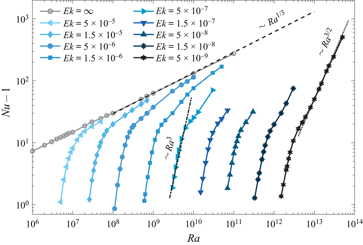
As demonstrated in figure 2, after the onset of convection ( $Nu>1$), at moderate $Ra$ in the rotation-dominated regime, the steep heat transfer scaling of $Nu-1\sim Ra^{3}$ as compared with the non-rotating cases is observed for $Ek\leq 10^{-6}$. With increasing $Ra$, the steep growth of $Nu-1$ with increasing $Ra$ gradually flattens. With further increase of $Ra$, the convective heat transport approaches the scaling about ${\sim }Ra^{1/3}$ for the classical regime of non-rotating RB convection for the corresponding $Ra$ (Grossmann & Lohse Reference Grossmann and Lohse2000). Interestingly, for the lowest $Ek= 5\times 10^{-9}$, after the steep heat transport scaling regime, the diffusion-free heat transfer scaling ${\sim }Ra^{3/2}$ is observed for the very high $Ra\geq 10^{13}$ (Song et al. Reference Song, Shishkina and Zhu2024). Obviously, in no-slip RRBC, there are several distinct heat transfer scaling regimes that are associated with different combinations of $Ra$ and $Ek$ ranges. In contrast to this, previous numerical results of RRBC with stress-free boundary conditions showed only the diffusion-free heat transfer scaling of ${\sim } Ra^{3/2}$ in almost the whole studied range of $Ra$ and $Ek$ (Stellmach et al. Reference Stellmach, Lischper, Julien, Vasil, Cheng, Ribeiro, King and Aurnou2014; Plumley et al. Reference Plumley, Julien, Marti and Stellmach2017; Plumley & Julien Reference Plumley and Julien2019). This suggests that in the presence of no-slip boundaries, the viscous (Ekman) BL dynamics has a significant impact on the heat transfer properties in RRBC (Kunnen et al. Reference Kunnen, Stevens, Overkamp, Sun, van Heijst and Clercx2011; Stellmach et al. Reference Stellmach, Lischper, Julien, Vasil, Cheng, Ribeiro, King and Aurnou2014; Kunnen et al. Reference Kunnen, Ostilla-Mónico, van der Poel, Verzicco and Lohse2016; Plumley et al. Reference Plumley, Julien, Marti and Stellmach2016). Specifically, there is a growth of thermal perturbations that lead to vertical and horizontal motions. The vertical velocity amplification can be viewed as an effective Ekman pumping boundary condition that yields a much steeper variation of $Nu$ with $Ra$ than the rotation-dominated regime without the Ekman BL (Kunnen et al. Reference Kunnen, Stevens, Overkamp, Sun, van Heijst and Clercx2011; Stevens, Clercx & Lohse Reference Stevens, Clercx and Lohse2013; Julien et al. Reference Julien, Aurnou, Calkins, Knobloch, Marti, Stellmach and Vasil2016; Kunnen et al. Reference Kunnen, Ostilla-Mónico, van der Poel, Verzicco and Lohse2016; Plumley et al. Reference Plumley, Julien, Marti and Stellmach2016; Aguirre Guzmán et al. Reference Aguirre Guzmán, Madonia, Cheng, Ostilla-Mónico, Clercx and Kunnen2020; Ecke & Shishkina Reference Ecke and Shishkina2023). However, how the BL dynamics affects the heat and momentum transfer scaling relations in different flow regimes of the RRBC requires detailed investigation.
Dimensionless convective heat transport  $Nu-1$ as a function of Rayleigh number $Ra$ for different Ekman numbers $Ek$, as obtained in the DNS. The black dashed line represents the heat transfer scaling relation of $Nu-1 \sim Ra^{1/3}$ for non-rotating RB convection in the classical regime, the dash-dotted line represents the steep heat transfer scaling of $\sim Ra^{3}$ and the dotted line represents the geostrophic turbulence heat transfer scaling of $\sim Ra^{3/2}$. Different symbols represent different $Ek$ and the colour of the lines and symbols reflects the rotation rate (darker with smaller $Ek$).
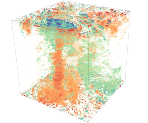
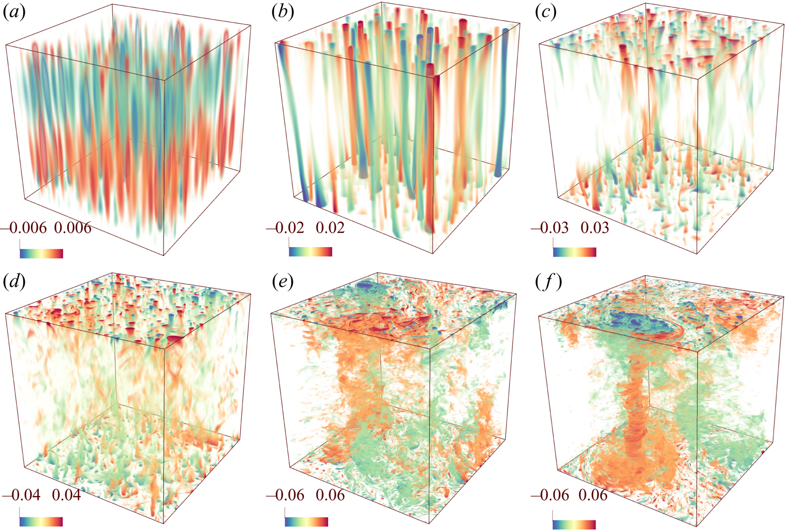
In order to illustrate the distinct flow regimes discussed above, we show the typical flow structures of RRBC. As depicted in figure 3, at the lowest  $Ek=5\times 10^{-9}$, with increasing $RaEk^{4/3}$, the flow undergoes in sequence cells, Taylor columns, plumes, geostrophic turbulence and the gradually enhanced formation of large-scale vortices (Julien et al. Reference Julien, Rubio, Grooms and Knobloch2012b; Stellmach et al. Reference Stellmach, Lischper, Julien, Vasil, Cheng, Ribeiro, King and Aurnou2014; Kunnen Reference Kunnen2021). Obviously, there are two important features of the flow structures in rotation-dominated RB convection: firstly, the flows are dominated by the vertically aligned structures in the cells, columns and plumes regimes where the geostrophic balance is predominant; secondly, in contrast to non-rotating RB convection where a large-scale circulation spans across the bottom and top walls in the flow field, the flow displays convective motions that have a smaller length scale as compared with the domain size. It should be noted that figure 3 shows only the typical flow structures of the rotation-dominated regime. With further increase of $Ra$, the flow will undergo transition into the buoyancy-dominated regime. To look at these flow structures, we refer to figure 3 of Cheng et al. (Reference Cheng, Madonia, Guzmán and Kunnen2020) or figure 1 of Ecke & Shishkina (Reference Ecke and Shishkina2023).
Thermal fluctuations  $\theta -\langle \theta \rangle$ showing (a) cells at $RaEk^{4/3}=12.82$, (b) the Taylor columns at $RaEk^{4/3}=21.37$, (c) plumes at $RaEk^{4/3}=42.75$, (d) geostrophic turbulence at $RaEk^{4/3}=85.50$, (e) weak large-scale vortices at $RaEk^{4/3}=256.50$ and (f) strong large-scale vortices at $RaEk^{4/3}=427.49$ as obtained in the DNS for $Ek=5\times 10^{-9}$. The domains have been stretched horizontally by a factor of $8$ for clarity. Everywhere, $\langle \cdots \rangle$ denotes the average in time and over horizontal cross-sections.
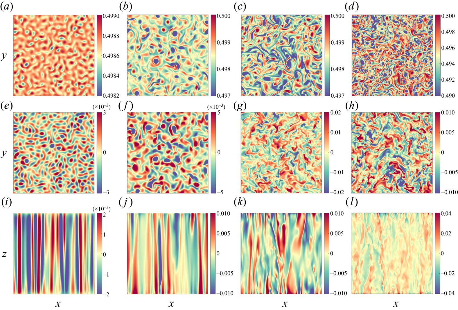
To further characterize the flow phenomenology of these distinct flow regimes (except for the large-scale vortices, for which we refer to Guervilly et al. Reference Guervilly, Hughes and Jones2014; de Wit et al. Reference de Wit, Guzmán, Clercx and Kunnen2022), the horizontal and vertical cross-sections of near-wall and bulk flow dynamics have been assessed and shown in figure 4. The spatial characteristics of these rotation-dominated flow regimes are consistent with previous numerical results of the asymptotically reduced model for quasigeostrophic convection with  $Pr=1$ (Oliver et al. Reference Oliver, Jacobi, Julien and Calkins2023) and similar to the DNS results with other $Pr$ values demonstrated in Aguirre Guzmán et al. (Reference Aguirre Guzmán, Madonia, Cheng, Ostilla-Mónico, Clercx and Kunnen2022). Specifically, the temperature fluctuations near the wall regions are much stronger than in the middle height plane. In cellular and columnar regimes, the colder fluid parcels are concentrated in small regions that display nearly circle shapes and they are surrounded by hotter fluid, and vice versa (see figure 4a,b,e,f). This flow pattern is also known as the ‘shielding effect’ for Taylor columns (Sprague et al. Reference Sprague, Julien, Knobloch and Werne2006; Julien et al. Reference Julien, Rubio, Grooms and Knobloch2012b; Stellmach et al. Reference Stellmach, Lischper, Julien, Vasil, Cheng, Ribeiro, King and Aurnou2014). Moreover, the number of these concentrated regions reduce and their sizes become larger as the flow transition from cellular to columnar regimes. During this transition, the bottom–top connected columns get distorted with the loss of a perfect vertical coherence (also see figure 4i,j). In the plume regime (figure 4c,g,k), the flow is essentially chaotic in the bulk region, while some concentrated columnar regions can still be observed within the Ekman BLs. In the view of the $xz$ plane, most of the top–down connected hot and cold columns have lost their vertical coherences. In the geostrophic turbulence regime, more violent fluctuations of smaller spatial scales especially near the wall regions are observed (see figure 4d,h). Intriguingly, figure 4(l) shows that the flow is highly turbulent and almost independent from the vertical position in the bulk region, with very weak vertical coherence.
Instantaneous horizontal cross-sections ( $xy$ plane) of temperature fluctuations $\theta -\langle \theta \rangle$ at the edge of the bottom Ekman BL (a–d), mid-height (e–h) and vertical cross-sections ( $xz$ plane) (i–l) for selected cases of (a,e,i) cells ( $RaEk^{4/3}=12.82$), (b,f,j) Taylor columns ( $RaEk^{4/3}=21.37$), (c,g,k) plumes ( $RaEk^{4/3}=42.75$) and (d,h,l) geostrophic turbulence ( $RaEk^{4/3}=85.50$), for the smallest $Ek=5\times 10^{-9}$. For clarity, the $xz$ planes are stretched horizontally by a factor of $8$.
$8$.
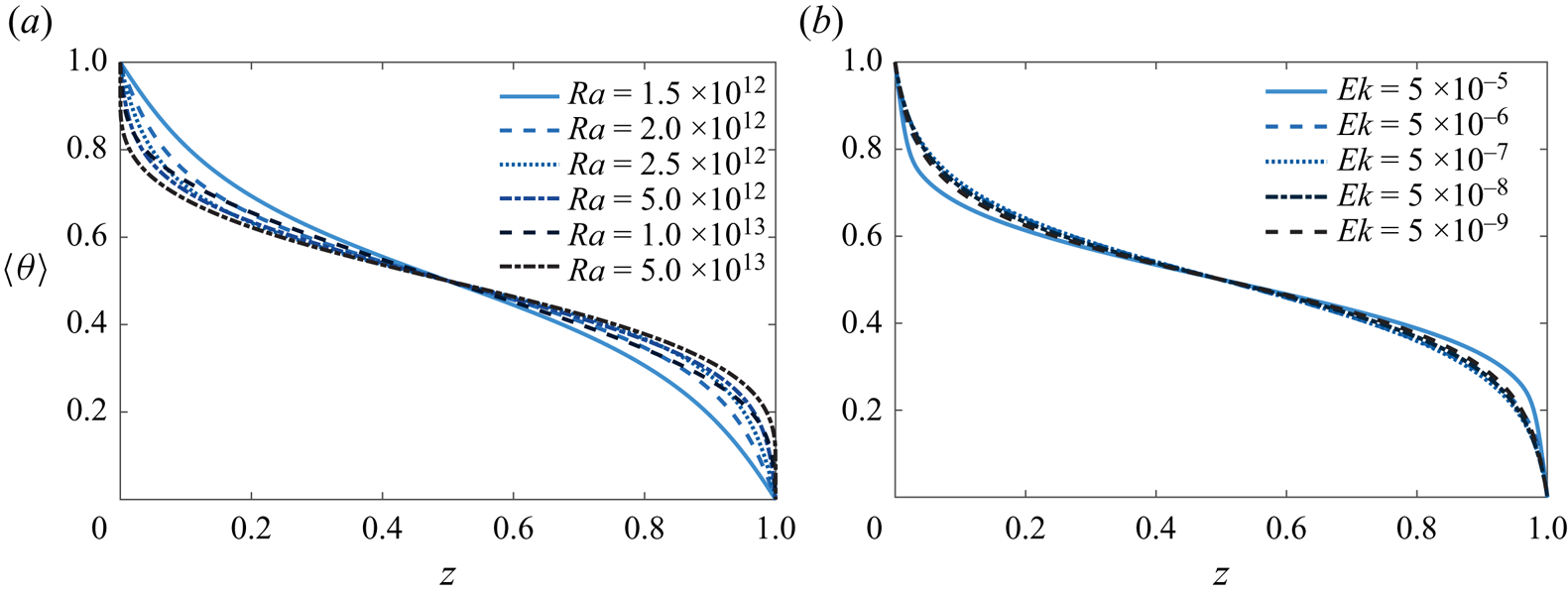
The insufficient mixing of the temperature at the middle height demonstrated above implies the obvious temperature gradients in the bulk region in RRBC (Boubnov & Golitsyn Reference Boubnov and Golitsyn1990; Julien et al. Reference Julien, Legg, McWilliams and Werne1996; Gillet & Jones Reference Gillet and Jones2006; Kunnen, Geurts & Clercx Reference Kunnen, Geurts and Clercx2010; Julien et al. Reference Julien, Rubio, Grooms and Knobloch2012b; King et al. Reference King, Stellmach and Aurnou2012; Stellmach et al. Reference Stellmach, Lischper, Julien, Vasil, Cheng, Ribeiro, King and Aurnou2014; Gastine et al. Reference Gastine, Wicht and Aubert2016). The time and horizontally averaged temperature profiles for different  $Ra$ and $Ek$ are elucidated in figure 5. Non-vanishing temperature gradients in the bulk regions are observed for all considered rotating cases. At a constant $Ek=5\times 10^{-9}$ (figure 5a), the increase of $Ra$ changes the temperature distribution toward the isothermal fluid bulk, with gradually thinner thermal BL thickness as will be discussed in the following part. However, as demonstrated in figure 5(b), the mean temperature profiles look similar even for several orders difference in $Ek$, if the heat transport ( $Nu$) is similar. This means that these flows have comparable fluctuation-induced heat fluxes $\langle w\theta ^{\prime }\rangle$ in the bulk region.
Vertical profiles of the time and horizontally averaged temperature  $\langle \theta \rangle$ for (a) different $Ra$ and a fixed Ekman number $Ek=5\times 10^{-9}$ and (b) different Ekman numbers and similar Nusselt numbers $10.6\leq Nu \leq 12.3$.
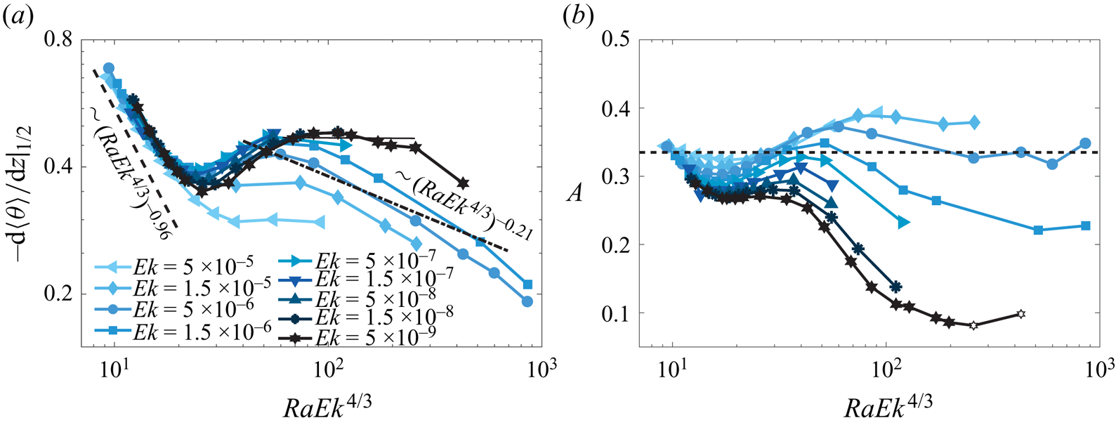
The temperature gradient measured at mid-height is frequently used for determining different regimes and flow transitions in RRBC (Stevenson Reference Stevenson1979; Julien et al. Reference Julien, Rubio, Grooms and Knobloch2012b; Stellmach et al. Reference Stellmach, Lischper, Julien, Vasil, Cheng, Ribeiro, King and Aurnou2014; Cheng et al. Reference Cheng, Madonia, Guzmán and Kunnen2020; Aguirre Guzmán et al. Reference Aguirre Guzmán, Madonia, Cheng, Ostilla-Mónico, Clercx and Kunnen2022). As one can see, the mean temperature gradients at the middle height shown in figure 6(a) first decrease in the cellular and columnar regimes and then saturate for larger  $Ek>1.5\times 10^{-5}$. The decrease exponent is around $-0.86$, consistent with Aguirre Guzmán et al. (Reference Aguirre Guzmán, Madonia, Cheng, Ostilla-Mónico, Clercx and Kunnen2022) and slightly differ from the asymptotic scaling of $(RaEk^{4/3})^{-0.96}$ proposed by Julien et al. (Reference Julien, Rubio, Grooms and Knobloch2012b). For the smaller $Ek\leq 5\times 10^{-6}$, a slight increase of the mean temperature gradients instead of the saturation is obtained, which corresponds to a transition to the plume regime (Nieves et al. Reference Nieves, Rubio and Julien2014). Similar mean temperature gradients were also observed by Zhong et al. (Reference Zhong, Stevens, Clercx, Verzicco, Lohse and Ahlers2009), Kunnen et al. (Reference Kunnen, Geurts and Clercx2010), Liu & Ecke (Reference Liu and Ecke2011), Horn & Shishkina (Reference Horn and Shishkina2014), Cheng et al. (Reference Cheng, Madonia, Guzmán and Kunnen2020) in both simulations and experiments, in agreement with predictions by Julien et al. (Reference Julien, Rubio, Grooms and Knobloch2012b) for the transition from the plume regime to geostrophic turbulence regime. Here, we observe the flattened region at $80\leq RaEk^{4/3}\leq 250$ with $Ek=5\times 10^{-9}$ of the diffusion-free regime. However, it should be noted that only when the thermal deriving and rotation are sufficiently strong, the geostrophic turbulence regime can be observed for a wide range of $RaEk^{4/3}$. For $RaEk^{4/3}\geq 100$, all gradients decrease monotonically to the lowest value of about $0.2$, getting closer to zero value, which corresponds to the well-mixed isothermal bulk state of highly turbulent non-rotating convection. It should be noted that a saturated non-zero bulk gradient for geostrophic turbulence and its required transition to a zero gradient for buoyancy-dominated convection has been raised by Julien et al. (Reference Julien, Rubio, Grooms and Knobloch2012b) and later studied by Aguirre Guzmán et al. (Reference Aguirre Guzmán, Madonia, Cheng, Ostilla-Mónico, Clercx and Kunnen2022) and Hartmann et al. (Reference Hartmann, Yerragolam, Verzicco, Lohse and Stevens2023). The decrease slope is steeper than $-0.21$ for the so-called rotation-influenced turbulence observed in extensive water experiments with $Pr\approx 5.2$ by Cheng et al. (Reference Cheng, Madonia, Guzmán and Kunnen2020). In addition, to study the degree of anisotropy in different flow regimes, we plot the kinetic energy anisotropy as a function of $RaEk^{4/3}$ for each simulation in figure 6(b), where $A=u_z^2/(u_h^2+u_z^2)$ (Madonia et al. Reference Madonia, Guzmán, Clercx and Kunnen2023). In contrast to the almost isotropy of the flows measured in the experiments with $Pr\approx 5.2$ by Madonia et al. (Reference Madonia, Guzmán, Clercx and Kunnen2023), we obtain that the degree of anisotropy increases with stronger rotation in the cellular and columnar regimes. Note that the velocity was measured in experiments at the middle plane, while here, the volume-averaged velocity is considered, which could be an explanation for this discrepancy. For higher $Ek>5\times 10^{-6}$, when the flow undergoes a transition to the buoyancy-dominated regime, it becomes nearly isotropic. For the stronger rotation for $Ek\leq 5\times 10^{-6}$, the flow is more anisotropic as the flow undergoes a transition to the plume regime and/or geostrophic turbulence regime. This anisotropy is especially strong when the large-scale vortices form (see the last two open symbols).
(a) Temperature gradient at middle height as a function of  $RaEk^{4/3}$ for different $Ek$. The horizontal solid line denotes a flattened range of the smallest $Ek$. The dashed line represents the scaling of $(RaEk^{4/3})^{-0.96}$ proposed by Julien et al. (Reference Julien, Rubio, Grooms and Knobloch2012b), the dash-dotted line denotes the scaling of $(RaEk^{4/3})^{-0.21}$ for rotation-influenced turbulence demonstrated by Cheng et al. (Reference Cheng, Madonia, Guzmán and Kunnen2020) in experiments. (b) Kinetic energy anisotropy $A=u_z^2/(u_h^2+u_z^2)$ as a function of $RaEk^{4/3}$ for different $Ek$. The horizontal dashed line ( $A=1/3$) denotes isotropy.
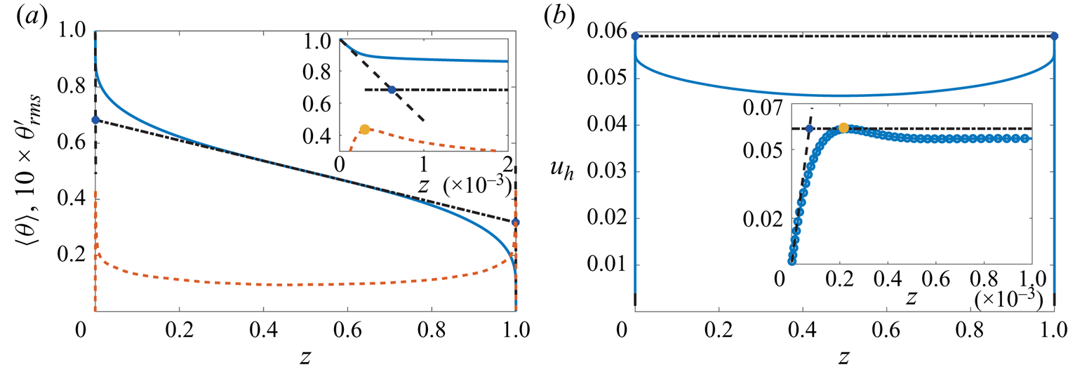
Before discussing the BL statistics, we first consider the definitions of thermal and viscous BLs, with two frequently used approaches: the slope and the maximum value methods (Verzicco & Camussi Reference Verzicco and Camussi1999; Breuer et al. Reference Breuer, Wessling, Schmalzl and Hansen2004; Gastine et al. Reference Gastine, Wicht and Aubert2016). The motivation to discuss the BL properties via two different definition methods are twofold: first, the different properties of the BL thickness and associated temperature drop within the BL based on these two common methods have not been well studied in RRBC until now; second, in such a broad parameter range, whether the scaling behaviours of the BL thickness defined by these two methods are similar or not is not clear, especially in the geostrophic turbulence regime. Specifically, as illustrated in figure 7(a), the slope method defines the thermal BL thickness  $\delta _\theta ^s$ as the depth where the linear fit to the mean temperature profile near the wall intersects the linear fit to the profile at mid-depth. The maximum value method defines the thermal BL thickness $\delta _\theta ^m$ as the average distance from the bottom and top walls to the location of the maximum value of the root mean square of the temperature fluctuations $\theta ^{\prime }=\theta -\langle \theta \rangle$ near each wall. Analogously, the slope method defines the viscous BL thickness $\delta _u^s$ as the distance from the wall where the linear fit to the horizontal velocity profile $u_h=\sqrt {\langle u_x^{2}+u_y^{2}\rangle }$ near the wall intersects with the horizontal line passing through the maximum of $u_h$ (see figure 7b); the maximum value method defines the viscous BL thickness $\delta _u^m$ as the average distance from the bottom and top walls to the maximum value of $\langle u_h\rangle$ near each wall.
Sketches to the definitions of the thermal (a) and the viscous (b) BL thicknesses, by example of  $Ra=5\times 10^{13}$ and $Ek=5\times 10^{-9}$. The shown solid lines are mean temperature $\langle \theta \rangle$ and horizontal velocity $\langle u_h\rangle$, respectively. The yellow dashed line is the root mean square of the temperature fluctuation (multiplied by 10 for clarity). The black dashed lines denote the tangent lines near the walls. The dash-dot lines denote (a) the tangent at middle height and (b) the horizontal passing through the maximum value of $\langle u_h\rangle$. The blue dots denote the intersects, i.e. the BL positions according to the slope method. The yellow dots denote the peak values, i.e. the BL positions according to the maximum value method. The insets show enlarged figures near the bottom plate.
The heat transport behaviour of RRBC is intimately related to the BL dynamics. In figure 8(a,b) we show the thermal BL thicknesses calculated via the two methods with the definitions described above. The values of the two types of the BL thicknesses show a similar trend to a monotonical decrease with the supercriticality  $RaEk^{4/3}$, and they show no sign of saturation for rapidly rotating cases, which is consistent with previous results for different $Pr$ (Julien et al. Reference Julien, Rubio, Grooms and Knobloch2012b). Moreover, Julien et al. (Reference Julien, Rubio, Grooms and Knobloch2012b) proposed that the relation $\delta _{\theta } \sim (RaEk^{4/3})^{-2}$ should hold for the turbulent state of rapidly RRBC. Here, this scaling relation can be locally observed for $50\lesssim RaEk^{4/3}\lesssim 200$ for the thermal BL, defined with the slope method. In turbulent non-rotating RB convection the thermal BL thickness is given by $\delta _{\theta } \approx (2Nu)^{-1}$ (Ahlers et al. Reference Ahlers, Grossmann and Lohse2009). As demonstrated in figure 8(c), in RRBC the relation of $\delta _{\theta } \approx (2Nu)^{-1}$ is also roughly held for the BL thickness defined by the slope method. This scaling relation for the maximum value defined thermal BL thickness shown in figure 8(d) is scattered for different $Ek$. In the compensated plots, the two BL thicknesses, $\delta _{\theta }^s$ and $\delta _{\theta }^m$, show different trends with the supercriticality in the rotation-dominated regime ( $RaEk^{4/3}\leq 20$). However, for both $\delta _{\theta }^s$ and $\delta _{\theta }^m$, short flattened ranges of $80\leq RaEk^{4/3}\leq 200$ are found for the smallest $Ek=5\times 10^{-9}$, which roughly corresponds to the geostrophic turbulence regime. At high $RaEk^{4/3}\geq 200$, the compensated values for both $\delta _{\theta }^s$ and $\delta _{\theta }^m$ begin to increase and gradually approach 1.
The dimensionless thermal BL thicknesses defined by (a) the slope method  $\delta _{\theta }^{s}$ and (b) the maximum value method $\delta _{\theta }^{m}$ as a function of $RaEk^{4/3}$, for different $Ek$. The dash-dot lines denote the scaling of $\delta _{\theta }\sim (RaEk^{4/3})^{-2}$ predicted by Julien et al. (Reference Julien, Rubio, Grooms and Knobloch2012b) for geostrophic turbulence. The dimensionless thermal BL thickness $\delta _{\theta }^{s}$ (c) and $\delta _{\theta }^{m}$ (d) vs $Nu$ for different $Ek$. The dash-dotted lines denote $\delta _{\theta }^{s}=0.3Nu^{-1}$ and $\delta _{\theta }^{m}=0.4Nu^{-1}$, respectively. The insets show the compensated plots with $(2Nu)^{-1}$.

Despite the different trends from the two thermal BL thickness definitions, the mean temperature drop within the thermal BL shown in figure 9 demonstrates similar behaviours with the supercriticality, in both cases. Specifically, it first decreases with  $RaEk^{4/3}$, then follows a short plateau and, in turn, increases as the flow approaches the buoyancy-dominated regime, where the mean temperature drop in the bulk is small. Specifically, in the cellular and columnar regimes ( $RaEk^{4/3}\leq 20$), the value of $\delta T(m)$ decreases dramatically from around 0.5 to 0.15. In contrast to the case $Pr=1$ reported in Julien et al. (Reference Julien, Rubio, Grooms and Knobloch2012b), an obvious plateau at $RaEk^{4/3}\approx 100$ is observed here for the plume regime and geostrophic turbulence regime for the smallest $Ek=5\times 10^{-9}$. Here, the temperature drop within the thermal BL, according to the maximum value definition, $\delta T(m)$, goes down and reaches the lowest value of around 0.1, which implies the very small BL contribution to the total mean temperature drop within the system. Hence, the heat transport in the turbulence regime of rapidly RRBC is dominated by the bulk dynamics. In particular, for the slope method based temperature drop, the scaling of $\delta T\sim (RaEk^{4/3})^{-1/2}$ is observed in this regime of rapidly RRBC ( $Ek= 5\times 10^{-9}$) as predicted by Julien et al. (Reference Julien, Rubio, Grooms and Knobloch2012b). Combining this with the valid relation $\delta _{\theta } \sim (RaEk^{4/3})^{-2}$ (see figure 8a) one obtains $2Nu\sim \delta T/\delta _{\theta }\sim (RaEk^{4/3})^{3/2}$. A closer look at the validity range for these scaling relations leads to a conclusion that the slope method defined thermal BL statistics reflects more accurately the diffusion-free regime of geostrophic turbulence.
The temperature drop within the thermal BL thicknesses defined by (a) the slope method and (b) the maximum value method, as a function of  $RaEk^{4/3}$, for different $Ek$. The dash-dot lines denote the scaling of $\delta T\sim (RaEk^{4/3})^{-1/2}$ predicted by Julien et al. (Reference Julien, Rubio, Grooms and Knobloch2012b) for geostrophic turbulence. The symbols have the same meaning as in figure 2.
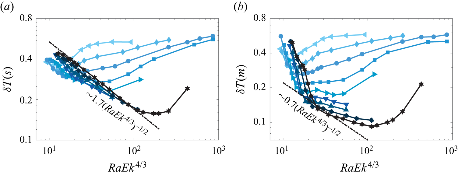
The kinetic BL in non-rotating RB convection is mainly determined by the shear induced by the large-scale circulation (Ahlers et al. Reference Ahlers, Grossmann and Lohse2009). Rotation dramatically changes the kinetic BL into the Ekman BL type (Greenspan Reference Greenspan1968), with the BL thickness  $\delta _u \sim 3Ek^{1/2}$. This relation can be obtained by considering a force balance between the Coriolis force and viscous force in the limit of $Ek \rightarrow 0$ (Greenspan Reference Greenspan1968). To verify this relation, we calculate the viscous BL thicknesses based on the definition sketched in figure 7. As shown in figure 10(a,b), the slope viscous BL thickness $\delta _{u}^s$ is almost an order of magnitude smaller than $\delta _{u}^m$, calculated with the maximum value method. This has also been reported by Hartmann et al. (Reference Hartmann, Yerragolam, Verzicco, Lohse and Stevens2023), where the slope method defined viscous BL thickness is understood as the thickness of a pseudo shear BL. The difference between the two definitions also suggests that they might have slightly different physical meanings. Interestingly, for each $Ek$, the values of $\delta _{u}^s$ and $\delta _{u}^m$ remain almost constant and slightly change with $Ra$. The insets in figure 10(a,b) show that both definitions of the Ekman BL thicknesses follow the theoretical scaling of $\delta _u \sim Ek^{1/2}$, especially in the rotation-dominated regime ( $RaEk^{4/3}\lesssim 300$). Beyond this range, $\delta _{u}^s$ shows a slight decrease and $\delta _{u}^m$ shows a slight increase. It should be noted that the $\delta _{u}^m/Ek^{1/2}\approx 3$, which is in excellent agreement with the theoretical prefactor proposed by Greenspan (Reference Greenspan1968).
The dimensionless viscous BL thicknesses defined by (a) the slope method  $\delta _{u}^{s}$ and (b) the maximum value method $\delta _{u}^{m}$ as functions of $Ek$ for different $Ra$. The dash-dotted lines denote $\delta _{u}^{s}=1.25Ek^{1/2}$ and $\delta _{u}^{m}=3Ek^{1/2}$ in (a) and (b), respectively. The insets show the compensated plots with $Ek^{1/2}$ for $\delta _{u}^{s}$ (a) and $\delta _{u}^{m}$ (b) as functions of $RaEk^{4/3}$, for different $Ek$.
$Ek$.

4. Heat, momentum transport, convective length scale scalings
In this section the global and local heat and momentum transport as well as the characteristic convective length scale scaling relations of RRBC are analysed, with particular emphasis on the local  $Re$ and $Ro$ scaling behaviours in the bulk and within the Ekman BL regions. It should be noted that in non-rotating RB convection, there exists a large-scale circulation with a single typical length scale $L$, determined by the container and the velocity scale $U$ (Grossmann & Lohse Reference Grossmann and Lohse2000). In RRBC, as shown in figure 3, the typical flow structures vary from vertically aligned cells and columns to plumes, geostrophic turbulence and/or large-scale vortices. As suggested by Guervilly et al. (Reference Guervilly, Hughes and Jones2014, Reference Guervilly, Cardin and Schaeffer2019) and Maffei et al. (Reference Maffei, Krouss, Julien and Calkins2021), in order to accurately characterize the amplitude of convective motions, the vertical fluctuation velocity $u=\sqrt {\langle u_z ^2\rangle }$ is frequently used as the typical velocity scale to define the Reynolds number ( $Re=uL/\nu$), which denotes the value obtained by time and the full volumetric average (Hawkins et al. Reference Hawkins, Cheng, Abbate, Pilegard, Stellmach, Julien and Aurnou2023).
First, we recall the two important force balances that determine various heat and momentum transfer scaling relations in RRBC. On the one hand, the balance of the viscous, buoyancy and Coriolis forces, i.e. the so-called VAC balance, leads to the onset length scale of  $\ell _o \sim Ek^{1/3}$ and the following momentum transfer scaling (Aurnou et al. Reference Aurnou, Horn and Julien2020; Hawkins et al. Reference Hawkins, Cheng, Abbate, Pilegard, Stellmach, Julien and Aurnou2023; Madonia et al. Reference Madonia, Guzmán, Clercx and Kunnen2023):
 \begin{equation} Re_{VAC}\sim Ra^{1/2}(Nu-1)^{1/2}Pr^{{-}1}Ek^{1/3}. \end{equation}
On the other hand, the balance of the Coriolis and inertial forces leads to  $\ell _i \sim (u/2\varOmega L)^{1/2}=Ro^{1/2}$, proposed for the case when the viscosity effects are negligible in a fully developed turbulent state. The balance of CIA forces gives rise to
 \begin{equation} Re_{CIA}\sim Ra^{2/5}(Nu-1)^{2/5}Pr^{{-}4/5}Ek^{1/5}. \end{equation}
 Based on our extensive DNS data for  $Pr=1$, we can check the above $Re_{VAC}$ and $Re_{CIA}$ scaling relations for various flow regimes. As demonstrated in figure 11(a,b), the DNS data are in a good agreement with both scaling relations for the whole parameter range. The best fit of the VAC scaling is $Re=(0.33\pm 0.01)Re_{VAC}^{1.12\pm 0.005}$ and the best fit of the CIA scaling is $Re=(0.43\pm 0.02)Re_{CIA}^{1.00\pm 0.005}$. In order to determine which force balance matches the present data better, we present compensated plots for these two $Re$ scalings in figure 11(c,d). A broad flattened range of $8\leq RaEk^{4/3}\leq 100$ is observed in figure 11(c), while only a very narrow flattened range of $50\leq RaEk^{4/3}\leq 100$ is seen in figure 11(d), indicating that the VAC-based $Re$ scaling agrees with the present data better than the CIA-based $Re$ scaling. Indeed the plateau range for the geostrophic turbulence regime in figure 11(d) is very limited. The reason could be the formation of large-scale vortices in the geostrophic turbulence regime with larger $RaEk^{4/3}\geq 100$, which is associated with an additional increase of $Re$ due to the inverse energy cascade (Julien et al. Reference Julien, Knobloch, Rubio and Vasil2012a,Reference Julien, Rubio, Grooms and Knoblochb; Wedi et al. Reference Wedi, Moturi, Funfschilling and Weiss2022). Here, a prefactor of about 2 is found for this flattening range for the VAC-based $Re$ scaling relation (4.1), and the valid range of CIA-based $Re$ scaling has a prefactor close to 1. The prefactors are consistent with the results of VAC- and CIA-based $Ro$ scaling reported in Hawkins et al. (Reference Hawkins, Cheng, Abbate, Pilegard, Stellmach, Julien and Aurnou2023).
(a) Plot of  $Re$ vs $Re_{VAC}$, where the best fit dashed line is given as $Re=(0.33\pm 0.01)Re_{VAC}^{1.12\pm 0.005}$; (b) $Re$ vs $Re_{CIA}$, where the best fit dashed line is $Re=(0.43\pm 0.02)Re_{CIA}^{1.00\pm 0.005}$. (c) The compensated plots of $Re/Re_{VAC}$ and (d) $Re/Re_{CIA}$ vs $RaEk^{4/3}$.

It should be noted that the above  $Re_{VAC}$ and $Re_{CIA}$ scaling relations contain the convective heat transport of $Nu-1$, which is a global response parameter of the thermal convection system. In order to determine the $Re_{VAC}$ and $Re_{CIA}$ scaling upon the control parameters, the convective heat transport $Nu-1$ scaling should be first determined. As it was shown in previous studies, the heat transport scaling varies dramatically in different flow regimes and the scaling exponent changes smoothly during the transition. We assume that there are three main options for the convective heat transfer $Nu-1$ dependence upon the control parameters for RRBC. First, for the columnar regime of RRBC with no-slip bottom and top walls, based on extensive measurements of the vertical mean temperature profile, Boubnov & Golitsyn (Reference Boubnov and Golitsyn1990) derived a steep heat transfer scaling of
 \begin{equation} Nu-1\sim (Ra/Ra_c)^{3}\sim Ra^{3}Ek^{4}. \end{equation}
This scaling was also proposed by King et al. (Reference King, Stellmach and Aurnou2012) using the marginal stability argument for the thermal BL. This is an analogy of the Malkus's theory for non-rotating RB convection (Malkus Reference Malkus1954).
Second, in the rotation-dominated geostrophic turbulence regime, under the assumption that the dimensional heat flux  $q$ is independent of the diffusive fluid properties $\nu$ and $\kappa$, along with the further assumption that the heat flux might only depend on the supercriticality $Ra/Ra_c$ (Julien et al. Reference Julien, Knobloch, Rubio and Vasil2012a), one can derive the following diffusivity-free heat transport scaling:
 \begin{equation} Nu-1\sim (Ra/Ra_c)^{3/2}\sim Ra^{3/2}Ek^{2}Pr^{{-}1/2}. \end{equation}
Using the CIA force balance analysis, Stevenson (Reference Stevenson1979), Gillet & Jones (Reference Gillet and Jones2006) and Aurnou et al. (Reference Aurnou, Horn and Julien2020) also derived the above asymptotic heat transport scaling relation. The inviscid heat transfer scaling of (4.4) was also derived by Julien et al. (Reference Julien, Knobloch, Rubio and Vasil2012a) using asymptotically reduced equations for  $Ek\rightarrow 0$ (Sprague et al. Reference Sprague, Julien, Knobloch and Werne2006).
At last, with increasing thermal driving force, the flow approaches the buoyancy-dominated regime (also see figure 2), where the heat transfer follows the classical scaling for non-rotating RB convection for the considered  $Ra$ and $Pr$,
$Pr$,
 \begin{equation} Nu-1 \sim Ra^{1/3}; \end{equation}
see Malkus (Reference Malkus1954) and Grossmann & Lohse (Reference Grossmann and Lohse2000).
Before we insert the convective heat transport scaling into the momentum scaling relations (4.1), (4.2) to obtain the  $Re$ scaling, we first verify it. As demonstrated in figure 12(a), where $Nu-1$ is plotted versus the supercriticality $RaEk^{4/3}$, the steep heat transfer scaling (4.3) and the diffusion-free scaling (4.4) are observed in the present dataset, as also elucidated in Song et al. (Reference Song, Shishkina and Zhu2024) for the data for $Ek\leq 1.5\times 10^{-7}$. Specifically, for the cellular and columnar regimes for $10\leq RaEk^{4/3}\leq 30$, the steep heat transfer scaling is broadly observed for almost all $Ek$ considered here; while the diffusion-free heat transport scaling is observed only for the two smallest $Ek\leq 1.5\times 10^{-8}$ for $70\leq RaEk^{4/3}\leq 300$. However, as suggested by Ecke (Reference Ecke2015), the heat transport data can also be considered from the perspective of weakly nonlinear theory. To this end, we also plot the data with $\epsilon =Ra/(8.7RaEk^{4/3})-1$ in figure 12(b). Similar results are obtained in Ecke (Reference Ecke2015): the steep heat transport scaling shown in figure 12(a) can be well fitted using the weakly nonlinear theory leading to $Nu-1\approx 2.2\epsilon +3.5\epsilon ^{2}$ or $Nu-1\approx 5\epsilon ^{1.4}$. However, for $\epsilon \leq 0.3$, the coefficient for the weakly nonlinear expansion shows a strong dependence on $Ek$. For high $\epsilon >10$, the diffusion-free heat transport scaling of $Nu-1\approx 1.8\epsilon ^{1.5}$ is achieved for the two smallest $Ek\leq 1.5\times 10^{-8}$. The comparison between these two ways demonstrates the substantial differences of the scaling relations for the low $\epsilon <10$ and similar results for higher $\epsilon >10$.
Convective heat transport  $Nu-1$ versus (a) the supercriticality $RaEk^{4/3}$ and (b) the $\epsilon =Ra/(8.7Ek^{-4/3})-1$ for all the DNS data shown in figure 2. The dashed line in (a) denotes the steep heat transfer scaling of $Nu-1\sim 0.001Ra^{3}Ek^{4}$ and the dash-dotted line the asymptotic heat transfer scaling of $Nu-1\sim 0.06Ra^{3/2}Ek^{2}$. The dashed line in (b) denotes the scaling of $Nu-1=5\epsilon ^{1.4}$, the solid line $Nu-1= 2.2\epsilon +3.5\epsilon ^{2}$ proposed by Ecke (Reference Ecke2015), and the dash-dotted line the asymptotic heat transfer scaling of $Nu-1\sim 1.8\epsilon ^{1.5}$.
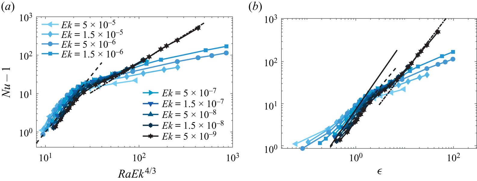
By inserting the above convective heat transfer scaling relations (4.3), (4.4), (4.5) into the momentum scaling relations (4.1), (4.2), we obtain the corresponding  $Re$ scaling relations for the specific flow regimes. Firstly, for the columnar regime, the viscosity-dependent heat and momentum transport scaling relations should be considered, as the flow is not turbulent. Hence, after we insert the steep heat transport relation (4.3) into the VAC-derived momentum transport scaling (4.1), we obtain
 \begin{equation} Re_{VAC_S}\sim Ra^{2}Ek^{7/3}Pr^{{-}1}=(RaEk^{4/3})^{2}Ek^{{-}1/3}Pr^{{-}1}. \end{equation}
In the geostrophic turbulence regime the viscous effects on the convective flow can be assumed negligible, thus, the diffusion-free heat transport relation (4.4) is substituted into the CIA-based momentum transport scaling (4.2), which leads to
 \begin{equation} Re_{CIA_D}\sim Ra^{1}Ek^{1}Pr^{{-}1}=(RaEk^{4/3})^{1}Ek^{{-}1/3}Pr^{{-}1}. \end{equation}
This is the diffusion-free momentum transport scaling relation for the geostrophic turbulence regime (Aurnou et al. Reference Aurnou, Horn and Julien2020; Hawkins et al. Reference Hawkins, Cheng, Abbate, Pilegard, Stellmach, Julien and Aurnou2023; Madonia et al. Reference Madonia, Guzmán, Clercx and Kunnen2023), which is also derived from the inviscid theory (Guervilly et al. Reference Guervilly, Cardin and Schaeffer2019).
In the buoyancy-dominated regime for moderate  $Ra$, where the viscous and inertia effects cannot be neglected, both the VAC- and CIA-based momentum transport scaling relations might work. To this end, taking the classical heat transport relation (4.5) for the non-rotating case and the VAC momentum transport scaling (4.1) leads to
 \begin{equation} Re_{VAC_C}\sim Ra^{2/3}Ek^{1/3}Pr^{{-}1}=(RaEk^{4/3})^{2/3}Ek^{{-}5/9}Pr^{{-}1}. \end{equation}
The insert to the CIA momentum transport scaling (4.2) gives rise to
 \begin{equation} Re_{CIA_C}\sim Ra^{8/15}Ek^{1/5}Pr^{{-}4/5}=(RaEk^{4/3})^{8/15}Ek^{{-}23/45}Pr^{{-}4/5}. \end{equation}
Recently, Hawkins et al. (Reference Hawkins, Cheng, Abbate, Pilegard, Stellmach, Julien and Aurnou2023) have derived equations (4.7), (4.9) and verified (4.9) via their extensive experimental and DNS results, which show a very good agreement with the local  $Re$ and $Ro$ scaling relations, which we discuss later.
The verification of the above derived global  $Re$ scaling relations are shown in figure 13 with the corresponding compensation shown as the insets. As expected and as shown in figure 13(a), the VAC-based viscous scaling agrees well with the data in the range of moderate supercriticality $RaEk^{4/3}\lesssim 20$, where the flows are in the cellular and columnar regimes. As demonstrated in figure 13(c), the CIA-based diffusion-free scaling matches the data for high supercriticality $30\lesssim RaEk^{4/3}\lesssim 200$, especially for the geostrophic turbulence regime of the two smallest Ekman numbers ( $Ek\leq 1.5\times 10^{-8}$). In addition, as shown in figure 13(b,d), both the VAC- and CIA-based $Re$ scaling relations derived from the classical $Nu-1\sim Ra^{1/3}$ serve as an upper bound scaling for the present data that approach the non-rotating state. However, as compared with the insets of figure 13(b,d), which force balance based scaling is most applicable to this regime is hard to determine.
The global  $Re$ scaling of (a) the VAC-derived scaling $Re_{VAC_S}\sim (RaEk^{4/3})^{2/3}Ek^{-5/9}$, (b) the VAC-derived scaling $Re_{VAC_C}\sim (RaEk^{4/3})^{2}Ek^{-1/3}$, (c) the CIA-derived diffusion-free scaling $Re_{CIA_D}\sim (RaEk^{4/3})^{1}Ek^{-1/3}$ and (d) the CIA-derived scaling $Re_{CIA_C}\sim (RaEk^{4/3})^{8/15}Ek^{-23/45}$. The best fit solid lines are $y=0.015x$, $y=0.1x$, $y=0.34x$ and $y=0.34x$ in (a), (b), (c) and (d), respectively. The inset in each plot shows the corresponding compensation of $Re$ with the $x$-coordinate scaling relation.

In order to further verify the agreement of VAC- and CIA-based  $Re$ scaling relations in the present DNS data with $Pr=1$, we follow Hawkins et al. (Reference Hawkins, Cheng, Abbate, Pilegard, Stellmach, Julien and Aurnou2023) and check the scaling relations for the local Reynolds number and Rossby number. Specifically, the local bulk Reynolds number is defined as $Re_l=u\ell /\nu =ReEk^{1/3}$, the local bulk Rossby number as $Ro_l=u/(2\varOmega \ell )=RoEk^{-1/3}$ and the local Rossby number in the Ekman BL as $Ro_{\delta _E}=u/(2\varOmega \delta _E)=RoEk^{-1/2}$. Here, the characteristic convective length scale is assumed to follow the onset length scale of $\ell_o \sim Ek^{1/3}$. For the VAC-based scaling relation $Re_{VAC_S}\sim (RaEk^{4/3})^{2}Ek^{-1/3}Pr^{-1}$, after the substitution of (4.6) into these local quantities, we obtain
 \begin{equation}
\left.\begin{array}{c@{}}
Re_l = ReEk^{1/3} \sim
Ra^{2}Ek^{8/3}Pr^{{-}1}=(RaEk^{4/3})^{2}Pr^{{-}1},\\ Ro_l
=(ReEk)Ek^{{-}1/3} \sim
Ra^{2}Ek^{3}Pr^{{-}1}=(RaEk^{4/3})^{2}Ek^{1/3}Pr^{{-}1},\\
Ro_{\delta_E} = (ReEk)Ek^{{-}1/2}\sim
Ra^{2}Ek^{17/6}Pr^{{-}1}=(RaEk^{4/3})^{2}Ek^{1/6}Pr^{{-}1}.
\end{array} \right\} \end{equation}
\begin{equation}
\left.\begin{array}{c@{}}
Re_l = ReEk^{1/3} \sim
Ra^{2}Ek^{8/3}Pr^{{-}1}=(RaEk^{4/3})^{2}Pr^{{-}1},\\ Ro_l
=(ReEk)Ek^{{-}1/3} \sim
Ra^{2}Ek^{3}Pr^{{-}1}=(RaEk^{4/3})^{2}Ek^{1/3}Pr^{{-}1},\\
Ro_{\delta_E} = (ReEk)Ek^{{-}1/2}\sim
Ra^{2}Ek^{17/6}Pr^{{-}1}=(RaEk^{4/3})^{2}Ek^{1/6}Pr^{{-}1}.
\end{array} \right\} \end{equation}
In turn, for the CIA-based scaling relation  $Re_{CIA_D}\sim (RaEk^{4/3})^{1}Ek^{-1/3}Pr^{-1}$, the substitution of (4.7) into these local quantities leads to
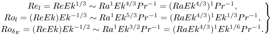 \begin{equation}
\left.\begin{array}{c@{}}
Re_l = ReEk^{1/3} \sim
Ra^{1}Ek^{4/3}Pr^{{-}1}=(RaEk^{4/3})^{1}Pr^{{-}1},\\ Ro_l =
(ReEk)Ek^{{-}1/3} \sim
Ra^{1}Ek^{5/3}Pr^{{-}1}=(RaEk^{4/3})^{1}Ek^{1/3}Pr^{{-}1},\\
Ro_{\delta_E} = (ReEk)Ek^{{-}1/2}\sim
Ra^{1}Ek^{3/2}Pr^{{-}1}=(RaEk^{4/3})^{1}Ek^{1/6}Pr^{{-}1}.
\end{array} \right\} \end{equation}
\begin{equation}
\left.\begin{array}{c@{}}
Re_l = ReEk^{1/3} \sim
Ra^{1}Ek^{4/3}Pr^{{-}1}=(RaEk^{4/3})^{1}Pr^{{-}1},\\ Ro_l =
(ReEk)Ek^{{-}1/3} \sim
Ra^{1}Ek^{5/3}Pr^{{-}1}=(RaEk^{4/3})^{1}Ek^{1/3}Pr^{{-}1},\\
Ro_{\delta_E} = (ReEk)Ek^{{-}1/2}\sim
Ra^{1}Ek^{3/2}Pr^{{-}1}=(RaEk^{4/3})^{1}Ek^{1/6}Pr^{{-}1}.
\end{array} \right\} \end{equation}
The above CIA-based asymptotic local  $Re$- and $Ro$-scaling relations (4.11) were proposed by Hawkins et al. (Reference Hawkins, Cheng, Abbate, Pilegard, Stellmach, Julien and Aurnou2023), but these asymptotic scalings were not verified since the diffusion-free heat transfer regime given by (4.4) was not attained in their dataset. In the cellular and columnar regimes, as demonstrated in figure 14(a–c), the local bulk $Re$, local bulk $Ro$ and local $Ro$ in the Ekman BL scaling relations (4.10) are in reasonable agreements with our data in the range of moderate supercriticality. On the other side, in the figure 14(d–f), the local scaling relations (4.11) also show decent agreements with our data for the geostrophic turbulence regime for small $Ek\leq 1.5\times 10^{-8}$. In addition, the corresponding compensated plots of figure 14 (not shown here) look very similar to the insets of figure 13, that show the compensated plots of global $Re$-scaling relations. Hence, the VAC-based ( $RaEk^{4/3}\lesssim 20$) and CIA-based ( $30\lesssim RaEk^{4/3}\lesssim 200$) local $Re$- and $Ro$-scaling relations work similarly well as demonstrated in figure 13.
The scaling relations for the local bulk Reynolds number  $Re_l=ReEk^{1/3}$ (a,d), local bulk Rossby number $Ro_l=RoEk^{-1/3}$ (b,e) and local Rossby number in the Ekman BL $Ro_{\delta _E}=RoEk^{-1/2}$ (c,f). The scaling relations in (a–c) are derived from the VAC- $Re$ scaling as (4.10) and the solid lines denote $y=0.014x$. The scaling relations in (d–f) are derived from the CIA- $Re$ scaling as (4.11) and the solid lines denote $y=0.35x$. The symbols have the same meaning as in figure 2.

It should be noted that the CIA force balance requires the characteristic convective length scale to follow the inertial length scale  $\ell_i \sim Ro^{1/2}$ (Aurnou et al. Reference Aurnou, Horn and Julien2020; Hawkins et al. Reference Hawkins, Cheng, Abbate, Pilegard, Stellmach, Julien and Aurnou2023; Madonia et al. Reference Madonia, Guzmán, Clercx and Kunnen2023). To this end, here we also use this inertial length scale to define the local Reynolds number as $Re_{l_i}=u\ell /\nu =ReRo^{1/2}$, local bulk Rossby number as $Ro_{l_i}=u/(2\varOmega \ell )=Ro^{1/2}$. The local Rossby number in the Ekman BL, $Ro_{\delta _E}$, remains unchanged. Hence, we have
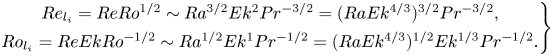 \begin{equation} \left.\begin{array}{c@{}}
Re_{l_i} = ReRo^{1/2} \sim
Ra^{3/2}Ek^{2}Pr^{{-}3/2}=(RaEk^{4/3})^{3/2}Pr^{{-}3/2},\\
Ro_{l_i}= ReEkRo^{{-}1/2} \sim
Ra^{1/2}Ek^{1}Pr^{{-}1/2}=(RaEk^{4/3})^{1/2}Ek^{1/3}Pr^{{-}1/2}.\\
\end{array} \right\} \end{equation}
\begin{equation} \left.\begin{array}{c@{}}
Re_{l_i} = ReRo^{1/2} \sim
Ra^{3/2}Ek^{2}Pr^{{-}3/2}=(RaEk^{4/3})^{3/2}Pr^{{-}3/2},\\
Ro_{l_i}= ReEkRo^{{-}1/2} \sim
Ra^{1/2}Ek^{1}Pr^{{-}1/2}=(RaEk^{4/3})^{1/2}Ek^{1/3}Pr^{{-}1/2}.\\
\end{array} \right\} \end{equation}
The above local  $Re_{l_i}$ and $Ro_{l_i}$ scaling relations, which are defined on the inertial length scale, are shown in figure 15(a,b). As expected, both local scalings show a decent agreement with our data for the geostrophic turbulence regime for small $Ek\leq 1.5\times 10^{-8}$. In order to assess which of the two length scales is more appropriate in the CIA-force balance regime, we compare the compensation plots of $Re_{l}$ vs $RaEk^{4/3}$ derived from (4.11) and $Re_{l_i}$ vs ( $RaEk^{4/3})^{2}$ derived in (4.12). Again, figure 15(c,d) shows a very similar trend and even the magnitude of the compensated results, which implies that the characteristic convective length scale might be co-scale for the valid range of $20\lesssim RaEk^{4/3}\lesssim 200$. Recently, Hawkins et al. (Reference Hawkins, Cheng, Abbate, Pilegard, Stellmach, Julien and Aurnou2023) have also demonstrated the co-scale of the CIA and VAC scalings based on their experimental and DNS data with $1.25\times 10^{-7}\leq Ek\leq 3\times 10^{-5}$ and $Pr\approx 6$. They have also theoretically elucidated that the onset and inertial length scales should co-scale if $Re_l\approx {O}(1)$ and $Ro_l\leq {O}(1)$, which we verify and discuss later.
Scaling relations of (a) the local bulk Reynolds number  $Re_{l_i}=ReRo^{1/2}$ and (b) the local bulk Rossby number $Ro_{l_i}=Ro^{1/2}$; see (4.12). The solid lines denote $y=0.2x$ and $y=0.6x$, respectively. The compensated plots of (c) the local bulk Reynolds number $Re_{l}$ vs $RaEk^{4/3}$, see (4.11), and (d) $Re_{l_i}$ vs ( $RaEk^{4/3})^{2}$, see (4.12).
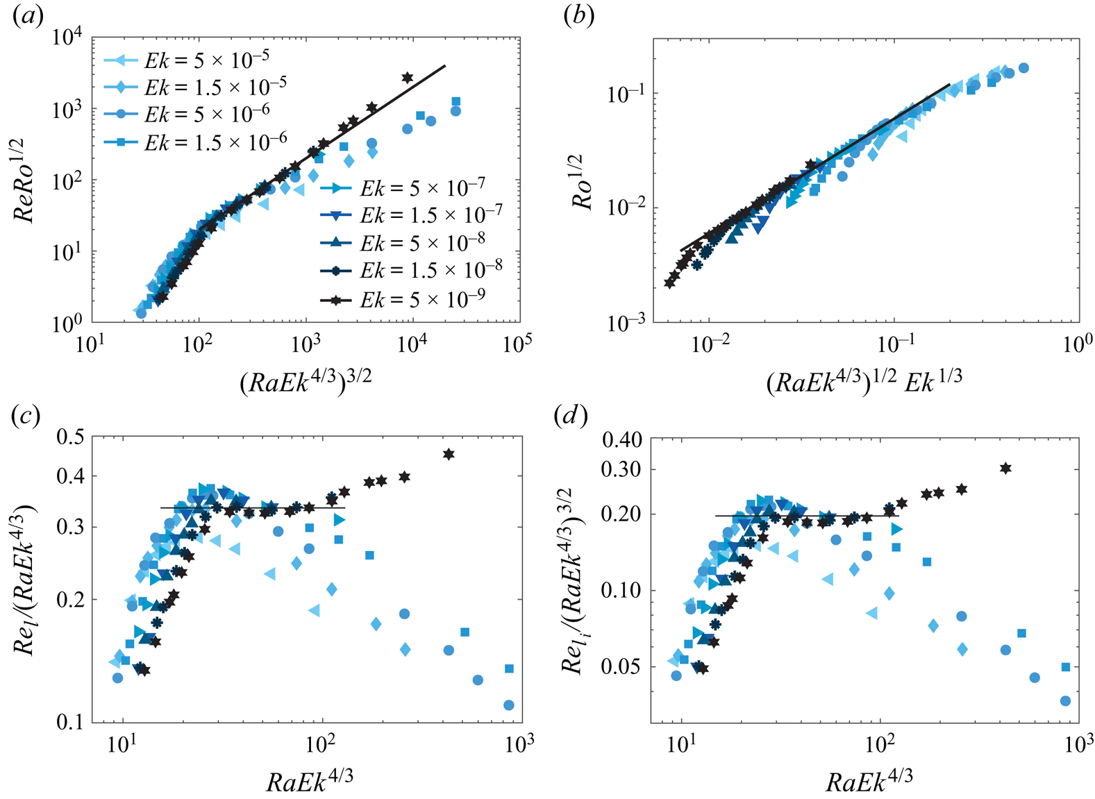
Another important characteristic of RRBC is the cross-axial length scale that plays an essential role in deriving the VAC- and CIA-related  $Nu$ and $Re$ scaling relations. As mentioned in the introduction, there are two important theoretical characteristic convective length scales in rotating convection: the onset critical length scale $\ell _o \sim Ek^{1/3}$ and the inertial convective length scale $\ell _i \sim (ReEk)^{1/2}=Ro^{1/2}$. Since the vertical velocity $u_z$ is used to quantify the convective flow motions in rotating convection, following Guervilly et al. (Reference Guervilly, Hughes and Jones2014, Reference Guervilly, Cardin and Schaeffer2019), Maffei et al. (Reference Maffei, Krouss, Julien and Calkins2021) we calculate the convective length scale $\ell$ as
 \begin{equation} \ell=\sum_{k_h} [\hat{u}_z(k_h)\hat{u}^*_z(k_h)]\left/\sum_{k_h} k_h [\hat{u}_z(k_h)\hat{u}^*_z(k_h)]\right.. \end{equation}
Here,  $\hat {u}_z(k_h)$ and $\hat {u}^*_z(k_h)$ are, respectively, the two-dimensional Fourier transforms of the vertical velocity and its complex conjugate at the middle height and $k_h\equiv (k_x^2+k_y^2)^{1/2}$ is the horizontal wavenumber. It should be noted that, based on recent studies on the convective length scale by Madonia et al. (Reference Madonia, Guzmán, Clercx and Kunnen2021), Song et al. (Reference Song, Shishkina and Zhu2024), the different definitions of the length scale could significantly affect the scaling range.
The convective length scale at the onset of convection scales as  $\ell \sim Ek^{1/3}$, as elucidated by the linear stability analysis (Chandrasekhar Reference Chandrasekhar1953, Reference Chandrasekhar1961). This relation is believed to hold also in the columnar and even plume regimes (Nieves et al. Reference Nieves, Rubio and Julien2014). This is supported by figure 16(a), where the data collapse and show a plateau at $RaEk^{4/3}\lesssim 20$, while for higher $RaEk^{4/3}\geq 50$, the data become scattered, indicating that this $Ek^{1/3}$ scaling does not hold in other flow regimes. However, for higher $RaEk^{4/3}\geq 20$, the convective length scale follows rather the scaling with $Ro^{1/2}=(ReEk)^{1/2}$, as demonstrated in figure 16(b). This implies that the convective length scale changes in the transition to different regimes. The scalings become clearly different for $RaEk^{4/3}\gtrsim 100$.
Dimensionless convective length scale  $\ell$ compensated with (a) $Ek^{1/3}$ and (b) $(ReEk)^{1/2}$ as functions of $RaEk^{4/3}$.
Finally, to compare the above derived heat and momentum transport scaling relations and our DNS data, we follow the procedure by Gastine et al. (Reference Gastine, Wicht and Aubert2016) and calculate the local effective exponents  $\alpha ^{eff}$ and $\beta ^{eff}$ for the convective heat transport, $Nu-1$, and momentum transport, $Re$ as functions of $Ra$:
$Ra$:
 \begin{equation} \alpha^{eff}=\frac{\partial \mathrm{ln} (Nu-1)}{\partial \mathrm{ln} Ra}, \quad \beta^{eff}=\frac{\partial \mathrm{ln} Re}{\partial \mathrm{ln} Ra}. \end{equation}
As demonstrated in figure 17(a),  $\alpha ^{eff}$ remains almost constant ( $\approx$0.33, solid line) for non-rotating convection. For all $Ek$ values considered here, $Ek$ holds for $0.3\leq \alpha ^{eff}\leq 5.2$. For any $Ek$ and relatively low values of $Ra$, one obtains $\alpha ^{eff}\geq 3$ that corresponds to the steep heat transport scaling regime elucidated in (4.3) and figure 12(a). From $Ek\le 5\times 10^{-6}$, the maximum value of $\alpha ^{eff}$ decreases monotonically with decreasing $Ek$, and $\alpha ^{eff}$ tends to saturate at a value with further reduction in $Ek$. Hence, more results with even lower $Ek$ are required to demonstrate the robustness of the scaling of $Nu-1\sim Ra^3$, which was derived theoretically. For higher $Ek\geq 5\times 10^{-6}$, with increasing $Ra$, the values of $\alpha ^{eff}$ first decrease sharply and then slowly approach $1/3$. While for $Ek\le 5\times 10^{-6}$, after the sharp drop, $\alpha ^{eff}$ increases slightly and in turn decreases to a value, which is gradually larger than $1/3$. For example, at the smallest $Ek=5\times 10^{-9}$, $\alpha ^{eff}\simeq 1.45$ at very high $Ra>10^{13}$, which shows the trend towards the asymptotic diffusion-free heat transport scaling exponent of 1.5 (dashed line) elucidated in (4.4) and figure 12.
Local effective exponent of (a)  $\alpha ^{eff}$ of $Nu-1\sim Ra^{\alpha ^{eff}}$ and (b) $\beta ^{eff}$ of $Re\sim Ra^{\beta ^{eff}}$ as functions of $Ra$, for different Ekman numbers. The solid and dashed lines in (a) denote $\alpha ^{eff}=1/3$ and $\alpha ^{eff}=1.5$, respectively, and in (b) denote $\beta ^{eff}=0.5$ and $\alpha ^{eff}=1.0$, respectively. The symbols have the same meaning as in figure 2.
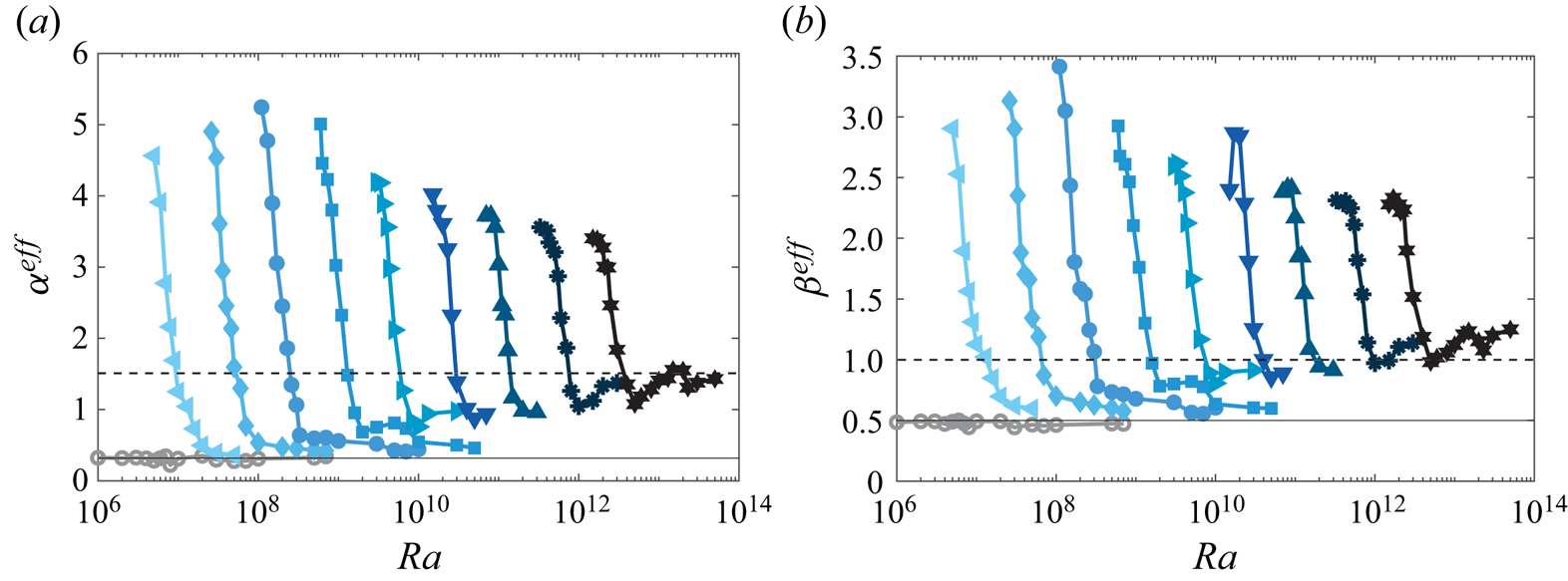
Intriguingly, in figure 17(b),  $\beta ^{eff}$ shows a very similar change in the trend as $\alpha ^{eff}$, but the magnitude is relatively smaller. For non-rotating convection, $\beta ^{eff}$ remains almost constant, around 0.5 (solid line). In the regime of the steep heat transport, the momentum transport scaling exponent $\beta ^{eff}$ decreases from $\approx 3$ to $\approx 2.3$ with increasing rotation rate. The value range of $2.3\leq \beta ^{eff}\leq 3.5$ in this regime is larger than the VAC-derived $Re$ scaling exponent of 2, see (4.6), which again requires further investigations at even lower $Ek$ to quantify the agreement of the VAC force balance in the specific parameter range of rotating convection. For higher $Ek\geq 5\times 10^{-6}$, beyond the steep heat transport regime, the values of $\beta ^{eff}$ also decrease sharply with $Ra$ and then slowly approach $0.5$ (solid line) for the non-rotating case. For small $Ek\leq 1.5\times 10^{-8}$, after the sharp drop, $\beta ^{eff}$ in turn increases a little bit to the value of about $1.2$, due to the formation of large-scale vortices in the flow. This value is slightly larger than 1 (dashed line), which corresponds to the asymptotic diffusion-free momentum transport scaling elucidated in (4.7) and figure 13(a).
5. Conclusions
Rotating Rayleigh–Bénard convection at  $Pr=1$ has been investigated via extensive three-dimensional DNS in the planar geometry with no-slip top and bottom and periodic lateral boundary conditions, for extreme rotation ( $Ek^{-1}$) and buoyancy ( $Ra$) parameters range. The DNS are performed in a broad parameter range with more than seven orders of $Ra$ and four orders of $Ek$, and up to $Ra=5\times 10^{13}$ down to $Ek=5\times 10^{-9}$. The extensive DNS has revealed the typical flow regimes of cellular flow, Taylor columns, plumes, geostrophic turbulence, large-scale vortices and also the buoyancy-dominated flows. The thermal and viscous BL statistics based on two different definitions are examined, these definitions are based on the slope method and maximum value method. It is shown that the dimensionless thermal BL thickness calculated by the slope method roughly follows $\delta _{\theta }\sim Nu^{-1}$ in a broad range. We demonstrate that the slope method thermal BL thickness shows more consistent scaling of $\delta _{\theta }\sim (RaEk^{4/3})^{-2}$, $\delta _{\theta }\sim (Nu)^{-1}$, $\delta T\sim (RaEk^{4/3})^{-1/2}$, which at last leads to $2Nu\sim \delta T/\delta _{\theta }\sim (RaEk^{4/3})^{3/2}$ for the geostrophic turbulence regime at very rapid rotation ( $Ek\leq 1.5\times 10^{-8}$), as predicted by Julien et al. (Reference Julien, Rubio, Grooms and Knobloch2012b). However, the mean temperature drops within the thermal BL defined by the two methods show a very similar trend versus $RaEk^{4/3}$ in different flow regimes. In addition, both the viscous BL thicknesses follow $\delta _{u}\sim Ek^{1/2}$ well in the rotation-dominated regime, but the maximum value viscous BL thickness agrees better with the theoretical scaling result of $\delta _{u}\sim 3Ek^{1/2}$, proposed by Greenspan (Reference Greenspan1968).
When the convective heat transport is plotted versus the supercriticality  $RaEk^{4/3}$, the steep heat transport scaling of $Nu-1\sim Ra^{3}Ek^{4}$ is observed for $RaEk^{4/3}\leq 30$, for almost all considered values of $Ek$ in the columnar regime. The steep heat transport scaling relation is replaced by the weakly nonlinear relation $Nu-1=2.2\epsilon +3.5\epsilon ^{2}$ or shallower scaling $Nu-1=5\epsilon ^{1.4}$ when plotted with $\epsilon =Ra/(8.7RaEk^{4/3})-1$, as proposed by Ecke (Reference Ecke2015). The asymptotic diffusion-free heat transport scaling relation $Nu-1\sim Ra^{3/2}Ek^{2} \sim \epsilon ^{3/2}$ is observed in the two different approaches. Both the VAC- and CIA-based $Re$ scaling relations are shown to agree well with the data for $Nu$ calculated from our DNS in a broad parameter range. After substituting the specific heat transport scaling relations into the $Re$ scaling relation derived from the VAC and CIA force balances, both the global and local VAC-based $Re$ scaling relations are shown to agree well with the data in the cellular and columnar regimes, while the CIA-based $Re$ scalings work well in the geostrophic turbulence regimes for a very rapid rotation, $Ek\leq 1.5\times 10^{-8}$. In addition, the convective length scale calculated based on the vertical velocity is demonstrated to scale well with the onset length scale of $Ek^{1/3}$ in the cellular and columnar regimes, while in the geostrophic turbulence regime it follows the inertia scale of $Ro^{1/2}$. Importantly, the achievement of the diffusion-free regime of geostrophic turbulence at extreme parameters (for very small $Ek\leq 1.5\times 10^{-8}$ and very large $Ra\geq 10^{13}$) is proved via examinations of different quantities. In order to increase the validity range of this diffusion-free regime, more extreme values of the parameters are needed. The local effective scaling exponents for the heat and momentum transport with respect to $Ra$ demonstrate a smooth change between the various distinct sub-regimes in RRBC. Finally, the proposed scaling relations that include also $Pr$ dependences, encourage future numerical and experimental investigations of the scaling relations with varying $Pr$.
$Pr$.
Acknowledgements
The authors are very grateful to R.E. Ecke and R.P.J. Kunnen for useful discussions and suggestions.
Funding
The authors acknowledge financial support from the Alexander von Humboldt Foundation Fellowship, Max Planck Society, and the German Research Foundation (DFG), grant nos Sh905/22, Sh405/16, 521319293 and 540422505. The authors gratefully acknowledge the computing time provided to them on the high-performance computer Lichtenberg at the NHR Centers NHR4CES at TU Darmstadt, funded by the Federal Ministry of Education and Research, and the state governments participating on the basis of the resolutions of the GWK for national high performance computing at universities, on the HPC systems of Max Planck Computing and Data Facility (MPCDF), on the HoreKa supercomputer funded by the Ministry of Science, Research and the Arts Baden-Württemberg and by the Federal Ministry of Education and Research, and on the GCS Supercomputer SuperMUC-NG at Leibniz Supercomputing Centre (LRZ).
Declaration of interests
The authors report no conflict of interest.
Appendix. Numerical parameters and grid resolutions
Summary of the quantities in the present DNS of RRBC (the non-rotating cases are not shown here, for which we refer to Zhu et al. Reference Zhu2018). All simulations are performed at  $Pr=1$. Here, $Ra$ is the Rayleigh number, $Ro_c$ is the convective Rossby number, $Re$ the Reynolds number, $Ek$ the Ekman number, $\varGamma =D/L$ the aspect ratio, where $D$ is the horizontal period and $L$ the domain height. The averaged Nusselt number $Nu$ is calculated from the $Nu$ values evaluated in five different ways: at the bottom and top plates, by volume averaging, from the kinetic energy and thermal dissipation rates. The $err$ denotes the maximum relative error between each two of these values. The averaging time interval is $\Delta t_{avg}$ (in the free-fall time units), and $err_h$ is the relative error between $Nu$ and the second half-averaging interval Nusselt number. The crudest space grid resolution in the bulk is $\varDelta _{V}/\eta$ (maximum value), where $\varDelta _{V}=(\varDelta _{x}\varDelta _{y}\varDelta _{z})^{1/3}$ is the mean grid width and $\eta$ is the mean Kolmogorov scale. The last column represents the grids mesh sizes used in the vertical ( $N_z$) and two horizontal ( $N_x$, $N_y$) directions. The other data for $Ek=1.5\times 10^{-7}, 5.0\times 10^{-8}, 1.5\times 10^{-8}, 5.0\times 10^{-9}$ are reported in Appendix A of Song et al. (Reference Song, Shishkina and Zhu2024).
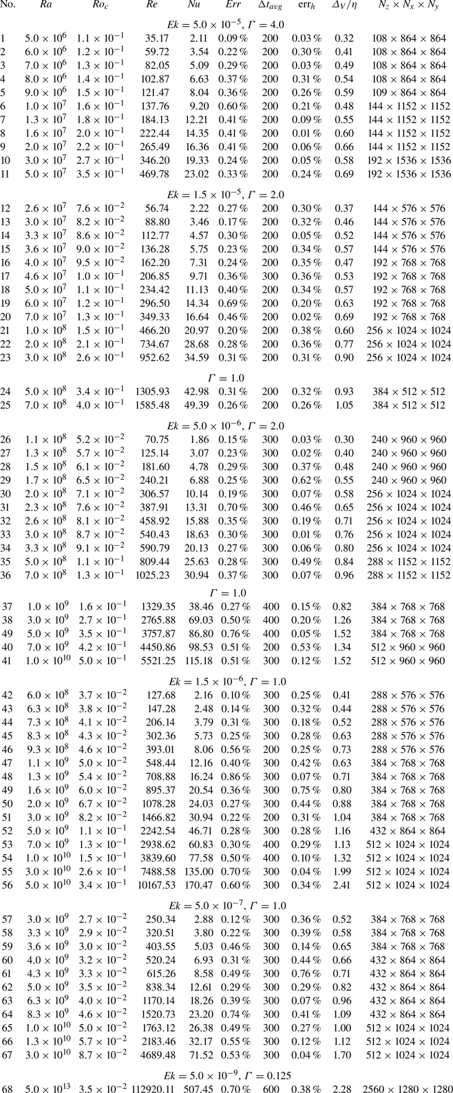


 Open access