


1. Introduction
Stochastic fluid processes have been used widely, with applications ranging from insurance [Reference Badescu14, Reference Bladt, Nielsen and Peralta22] and dam level modeling [Reference Loynes31] to telecommunications [Reference Anick, Mitra and Sondhi7] and queueing systems [Reference Asmussen9, Reference Karandikar and Kulkarni28, Reference Rogers36]. These models are often employed to study the dynamic behavior of systems in which resources are continuously depleted and replenished over time. This behavior is dictated by an underlying time-homogeneous Markov jump process. Although one-dimensional processes are well understood (see e.g. [Reference Latouche and Nguyen30] and references therein), the development and analysis of their multivariate counterparts present a significant challenge, owing to the need to account for complex interdependencies between the various processes. Such dependence plays a crucial role in these systems as it greatly affects their behavior and, consequently, the outcomes of any related decision-making processes.
A bivariate stochastic fluid process comprises two continuous-time processes. It is assumed that the fluid levels of each process fluctuate, owing to random events. The existing literature on bivariate stochastic fluid processes (see e.g. [Reference Bean and O’Reilly16, Reference O’Reilly and Scheinhardt32, Reference Rabehasaina35]) has primarily been focused on models driven by a fixed underlying Markov process, which may represent joint dynamics through coupled phase processes. While such models can capture certain forms of dependence, they do not accommodate ruin-dependent behavioral switches where both processes simultaneously undergo regime changes at a data-dependent random time. Although the components of the bivariate processes start as independent, the behavioral switch is ruin-dependent: at the first ruin, both processes transition simultaneously, creating dynamic coupling that cannot be captured by a fixed joint Markov chain. In some real-world applications, such dynamic switching is essential. For instance, in telecommunications, generalized processor sharing models redistribute the bandwidth of an empty buffer to active queues, causing an instantaneous rate increase for the remaining processes [Reference Parekh and Gallager33]. Similarly, in inventory management, reactive lateral transshipment policies dictate that when one location faces a stockout, inventory is diverted from a neighboring location, thereby accelerating the neighbor’s depletion rate [Reference Paterson, Kiesmüller, Teunter and Glazebrook34]. In this paper, the authors introduce a novel bivariate stochastic fluid process model that incorporates a ruin-dependent behavioral switch, which is triggered on the ruin of one of the processes. In this model, the bivariate process becomes a Markov jump process with randomized intensities.
In the context of a stochastic fluid process, ‘ruin’ refers to a situation where the fluid level of a process drops below level 0, thereby rendering the process unsustainable. In the model proposed here, the interdependence between the two processes alters when one process experiences ruin, signifying a behavioral switch. This ruin-dependent behavioral switch can be interpreted as a shift in operating conditions or decision-making rules within a real-world system. For example, within the realm of insurance risk, the ruin of one branch of an insurance company, like car insurance, experiencing difficulties might result in a premium adaptation for this and other branches. For financial investment strategies, the failure of one portfolio might prompt a shift toward a more conservative investment strategy for the remaining portfolio. In telecommunications, the failure of a node could trigger a rerouteing protocol to maintain service continuity by redirecting traffic to alternative nodes. Further examples occur in healthcare systems, where reaching capacity limit in one hospital would change the structure of arrivals in others.
Several studies of bivariate stochastic fluid processes have been conducted in various settings. Aalto and Scheinhardt [Reference Aalto and Scheinhardt1] and Kroese and Scheinhardt [Reference Kroese and Scheinhardt29] investigated the joint stationary distribution of on-off tandem fluid queues, i.e. stochastic fluid processes with two underlying states, where one component changes behavior whenever the other queue is idle (i.e. at level 0). Through operator theoretic considerations, this work was later extended [Reference O’Reilly and Scheinhardt32] to include the case with finite underlying states. Rabehasaina [Reference Rabehasaina35] computed the joint moments for the stationary distribution of a network of stochastic fluid processes whose inflow–outflow fluid dynamics between neighboring states is proportional to their queue size. Bean and O’Reilly [Reference Bean and O’Reilly16] considered the first return probability for the first coordinate of a bivariate stochastic fluid process in the event that the second coordinate’s level was below a certain threshold. In recent work [Reference Aksamit, O’Reilly and Palmowski2], methods have been developed to compute joint ruin probabilities for standard bivariate stochastic fluid processes through uniformization and mapping to quasi-birth-and-death processes.
However, none of these works involves the analysis of models with ruin-dependent behavioral switches, where the dynamics of both processes simultaneously undergo regime changes at the data-dependent random time when one process ruins. Furthermore, existing Laplace transform methods for unbounded bivariate fluid processes are designed to evaluate the distribution of the second fluid when the first hits zero from above for the first time. These methods do not accommodate settings where the second fluid may hit level zero before the first process does, creating problems when we wish to trigger behavioral switches based on whichever ruin occurs first. This ruin-dependent switching mechanism creates a fundamentally different dependency structure that requires new analytical approaches. Some related bivariate problems have been studied in the context of ruin processes with jumps [Reference Avram, Palmowski and Pistorius11–Reference Badescu, Cheung and Rabehasaina13, Reference Badila, Boxma, Resing and Winands15] for the case of proportional reinsurance with common shocks. While the authors of those works are able to compute the probability of ultimate joint ruin for a Cramér–Lundberg-type process, they do not analyze the law of the corresponding ruin times, a more challenging descriptor to study.
The primary objective of this research is to explore the effect of the ruin-dependent behavioral switch on the joint behavior of two stochastic fluid processes. We will develop the mathematical framework for the proposed model, analyze its properties, and derive closed-form expressions for key performance measures, specifically, the joint law of the ruin times of the coordinates. This descriptor is challenging to compute in a univariate setting (see e.g. [Reference Asmussen8, Reference Asmussen, Avram and Usabel10, Reference Stanford37]), and has been recently revisited in a bivariate Cramér–Lundberg risk setting through the use of Laguerre series [Reference Cheung, Lau, Willmot and Woo23].
The approach presented in this paper offers several key advantages over existing methods. First, traditional approaches rely on Laplace transforms that require numerical inversion, a computationally expensive step, especially for large state spaces (see e.g. [Reference Den Iseger26] and [Reference Telek38]). In contrast, this method produces explicit probability distributions through recursive matrix operations. Second, the developed matrix-analytic recursions have tractable computational complexity, involving only matrix multiplications and Hadamard products, while avoiding expensive operations, such as matrix inversion or exponentiation. Third, and importantly, the finite-time analysis does not require stability conditions: since first return probabilities over finite horizons are computed without relying on stationary distributions or limiting behavior, the processes may be unstable without affecting the validity of the results.
In contrast to the previous literature, the dependency in this case is triggered by ruin, rather than being associated with common shocks or the underlying processes. More importantly, this approach to computing descriptors of the bivariate process differs from that in the existing literature. The key challenge is that the behavioral switch occurs at the random time when one process first hits level zero, making the bivariate process non-Markovian after this event. The solution presented here is to approximate this switching time by observing the processes on a high-frequency Poisson grid and triggering the switch at the first Poisson observation after ruin occurs. This creates a family of approximating processes where the switching time is slightly delayed but controlled by the grid frequency.
We call such approximations compatible if they preserve the jump structure of the environmental processes: the states visited and transitions taken remain identical to the original process, with only the timing of the behavioral switch modified. The crucial property is that the approximation error, measured as the uniform distance between original and approximated paths over $[0,\infty)$
, is proportional to the time difference between the true ruin and the delayed switching time. As we increase the Poisson observation frequency (parameter
$[0,\infty)$
, is proportional to the time difference between the true ruin and the delayed switching time. As we increase the Poisson observation frequency (parameter $\gamma \to \infty$
), this delay vanishes, and the approximation converges to the original process. Importantly, each approximating process at finite
$\gamma \to \infty$
), this delay vanishes, and the approximation converges to the original process. Importantly, each approximating process at finite $\gamma$
is analytically tractable: we can compute its first return probabilities using matrix-analytic methods. In summary, this pathwise approximation framework allows us to study convergence through the simpler problem of convergence of random switching times, rather than through complex functional convergence arguments typically required in pathwise approximation theory (see e.g. [Reference Csörgö and Révész24]).
$\gamma$
is analytically tractable: we can compute its first return probabilities using matrix-analytic methods. In summary, this pathwise approximation framework allows us to study convergence through the simpler problem of convergence of random switching times, rather than through complex functional convergence arguments typically required in pathwise approximation theory (see e.g. [Reference Csörgö and Révész24]).
In essence, focusing on compatible pastings amounts to creating a scheme for randomly observing the behavioral switch. This can be paired with a Poissonian observation grid, which allows us to approximate the moment the ruined component reaches level 0. By conditioning on this Poissonian approximating switching point, we can reframe the bivariate problem in terms of one component that gets ruined first and another that undergoes a behavioral switch at a given Poissonian point in time. Measuring the time at which one component is ruined first amounts to computing its finite-time first return probabilities, which have been explored [Reference Amini, Minca and Peralta6, Reference Bean, Ngyuen and Poloni17] through the theory of n-bridges. The second component is considerably more challenging to tackle, and state-of-the-art algorithms for first return probabilities, whether for time-homogeneous or time-inhomogeneous stochastic fluid processes, do not apply. Here, we develop novel matrix-analytic and algorithmic considerations based on an extension of the theory of n-bridges that provide closed-form solutions for their first return probabilities. This methodology is thus a key ingredient, which could be extended in higher dimensions.
The organization of this paper is as follows. Section 2 defines the bivariate ruin-dependent stochastic fluid processes model. In Section 3, a family of pathwise approximations for these fluid processes, which are referred to as bivariate compatible pastings, is devised. Section 4 presents results regarding the convergence of bivariate compatible pastings, while Section 5 is devoted to calculating the first return probabilities. Section 6 presents a numerical illustration of the method, exploring convergence and the behavior of joint ruin probabilities. Proofs of the main theorems are provided in Section 7. Finally, Section 8 offers concluding remarks.
2. Bivariate model definition
We define a bivariate ruin-dependent stochastic fluid process $(F^{(1)}, F^{(2)})$
consisting of two fluid-level processes
$(F^{(1)}, F^{(2)})$
consisting of two fluid-level processes $F^{(1)}, F^{(2)}\,:\, [0,\infty) \to \mathbb{R}$
(unbounded state space) and their associated environmental processes
$F^{(1)}, F^{(2)}\,:\, [0,\infty) \to \mathbb{R}$
(unbounded state space) and their associated environmental processes $J^{(1)}, J^{(2)}$
, taking values in finite discrete state spaces. Each fluid level evolves according to
$J^{(1)}, J^{(2)}$
, taking values in finite discrete state spaces. Each fluid level evolves according to $F^{(k)}(t) = \int_0^t r^{(k)}(J^{(k)}(s)) \, \mathrm{d} s$
for
$F^{(k)}(t) = \int_0^t r^{(k)}(J^{(k)}(s)) \, \mathrm{d} s$
for $k \in \{1,2\}$
, where
$k \in \{1,2\}$
, where $r^{(k)}$
is a state-dependent reward (drift) function. The key feature of this model is a ruin-dependent behavioral switch: the processes evolve independently until the first time
$r^{(k)}$
is a state-dependent reward (drift) function. The key feature of this model is a ruin-dependent behavioral switch: the processes evolve independently until the first time $\tau^{[1]}$
that either
$\tau^{[1]}$
that either $F^{(1)}$
or
$F^{(1)}$
or $F^{(2)}$
hits level zero from above. At this moment, both environmental processes undergo a regime change, transitioning to new state spaces with altered dynamics. After the switch, the processes continue evolving independently on
$F^{(2)}$
hits level zero from above. At this moment, both environmental processes undergo a regime change, transitioning to new state spaces with altered dynamics. After the switch, the processes continue evolving independently on $\mathbb{R}$
but under the new regime. Our objective is to analyze the joint distribution of the ruin times
$\mathbb{R}$
but under the new regime. Our objective is to analyze the joint distribution of the ruin times $(\tau^{[1]}, \tau^{[2]})$
, where
$(\tau^{[1]}, \tau^{[2]})$
, where $\tau^{[1]}$
is the time when the first process ruins and
$\tau^{[1]}$
is the time when the first process ruins and $\tau^{[2]}$
is the time when both processes have ruined. The detailed construction is now provided, beginning with the univariate framework that forms the building blocks of the bivariate model.
$\tau^{[2]}$
is the time when both processes have ruined. The detailed construction is now provided, beginning with the univariate framework that forms the building blocks of the bivariate model.
Consider a discrete and finite jump space $\mathcal{E}$
, and a reward function
$\mathcal{E}$
, and a reward function $r\,:\,\mathcal{E}\mapsto\mathbb{R}\setminus\{0\}$
. Note that we assume nonzero fluid rates throughout. As is common in the literature, stochastic fluid process theory is typically developed first for nonzero rates, with zero rates handled through additional arguments (see e.g. [Reference Asmussen9] and [Reference Bean, Nguyen, Nielsen and Peralta18]). A univariate stochastic fluid process
$r\,:\,\mathcal{E}\mapsto\mathbb{R}\setminus\{0\}$
. Note that we assume nonzero fluid rates throughout. As is common in the literature, stochastic fluid process theory is typically developed first for nonzero rates, with zero rates handled through additional arguments (see e.g. [Reference Asmussen9] and [Reference Bean, Nguyen, Nielsen and Peralta18]). A univariate stochastic fluid process $F=\{F(t)\}_{t\ge 0}$
is defined as
$F=\{F(t)\}_{t\ge 0}$
is defined as
 \begin{equation}F(t)=\int_0^t r(J(s))\mathrm{d} s,\end{equation}
where J is a càdlàg (right continuous with left limits) jump process on $\mathcal{E}$
. For the sake of clarity, here we refer to F as the level process and to J as the environmental process (associated to F). We assume that J is Markovian, say driven by an intensity matrix
$\mathcal{E}$
. For the sake of clarity, here we refer to F as the level process and to J as the environmental process (associated to F). We assume that J is Markovian, say driven by an intensity matrix $\boldsymbol{A}$
; then the distribution of the univariate stochastic fluid process is completely characterized by the triplet
$\boldsymbol{A}$
; then the distribution of the univariate stochastic fluid process is completely characterized by the triplet $(\mathcal{E},\boldsymbol{A}, r)$
. Alternatively, we can describe the evolution of the 2-dimensional process (F, J) by means of a piecewise-deterministic Markov process (PDMP), introduced in [Reference Davis25], as follows. In this framework, the state space is
$(\mathcal{E},\boldsymbol{A}, r)$
. Alternatively, we can describe the evolution of the 2-dimensional process (F, J) by means of a piecewise-deterministic Markov process (PDMP), introduced in [Reference Davis25], as follows. In this framework, the state space is $\mathbb{R} \times \mathcal{E}$
and (F, J) is specified by the following local characteristics, where
$\mathbb{R} \times \mathcal{E}$
and (F, J) is specified by the following local characteristics, where $f\,:\, \mathbb{R} \times \mathcal{E} \to \mathbb{R}$
denotes a test function (assumed to be at least
$f\,:\, \mathbb{R} \times \mathcal{E} \to \mathbb{R}$
denotes a test function (assumed to be at least $C^1$
in its first argument to ensure differentiability).
$C^1$
in its first argument to ensure differentiability).
-
• A vector field $\mathcal{X}$
characterizing the flow of (F,J) between jumps takes the form this implies that on a holding time where J equals i, the process F moves uniformly in
\begin{align*} \mathcal{X}f(y,i) & = r(i)\frac{\partial f}{\partial y}(y,i),\qquad y\in\mathbb{R}, \, i\in \mathcal{E}; \end{align*}
$\mathbb{R}$
at a rate r(i). This ensures that F is a continuous process that evolves according to (2.1).
$\mathcal{X}$
characterizing the flow of (F,J) between jumps takes the form this implies that on a holding time where J equals i, the process F moves uniformly in
\begin{align*} \mathcal{X}f(y,i) & = r(i)\frac{\partial f}{\partial y}(y,i),\qquad y\in\mathbb{R}, \, i\in \mathcal{E}; \end{align*}
$\mathbb{R}$
at a rate r(i). This ensures that F is a continuous process that evolves according to (2.1).
-
• A jump intensity
$\lambda(y,i)=c_0$
for all
$(y,i)\in \mathbb{R}\times\mathcal{E}$
, where
$c_0$
is some fixed constant greater than or equal to
$\sup_{i\in\mathcal{E}}\left| A_{ii} \right|$
. -
• Jump kernels are of the form
The jump intensity and kernels jointly imply that, for J, a transition from i to j (
\begin{equation*} Q((y,i);\,(\mathrm{d} z, \mathrm{d} j))= \begin{cases} \dfrac{1}{c_0}A_{ij} & \mbox{if}\ y=z,\, i\neq j,\\ 1+\dfrac{1}{c_0}A_{ij} & \mbox{if}\ y=z,\, i=j,\\ 0 & \mbox{if}\ y\neq z. \end{cases} \end{equation*}
$i\neq j$
) within the time interval
$[t,t+\mathrm{d} t)$
occurs with probability
$(c_0\,\mathrm{d} t)(\tfrac{1}{c_0}A_{ij})=A_{ij}\,\mathrm{d} t$
. Similarly, in the same interval, the probability of no transition in the environmental process is
$(1-c_0\,\mathrm{d} t) + (c_0\,\mathrm{d} t)(1+ \tfrac{1}{c_0}A_{ii}) = 1 + A_{ii}\,\mathrm{d} t$
, confirming that J is driven by the intensity matrix
$\boldsymbol{A}$
.


We emphasize that this specific construction of J is rooted in the concept of uniformization (see for instance, [Reference van Dijk, van Brummelen and Boucherie39]), which fundamentally involves defining a jump process with switch times that occur on a Poissonian grid.
In the bivariate model of interest, we consider two univariate stochastic fluid processes, $F^{(k)}$
for
$F^{(k)}$
for $k\in\{1,2\}$
, each one driven by an environmental process
$k\in\{1,2\}$
, each one driven by an environmental process $J^{(k)}$
. Here, the processes
$J^{(k)}$
. Here, the processes $J^{(1)}$
and
$J^{(1)}$
and $J^{(2)}$
are not Markovian, but rather dependent on certain hitting times of the level processes
$J^{(2)}$
are not Markovian, but rather dependent on certain hitting times of the level processes $F^{(1)}$
and
$F^{(1)}$
and $F^{(2)}$
. To be precise, the level processes and their associated environmental processes are independent up to the first time that one of the fluid processes reaches zero. That is, for
$F^{(2)}$
. To be precise, the level processes and their associated environmental processes are independent up to the first time that one of the fluid processes reaches zero. That is, for $k\in\{1,2\}$
, we consider the jump space
$k\in\{1,2\}$
, we consider the jump space $\mathcal{E}^{(k)}$
, intensity matrix
$\mathcal{E}^{(k)}$
, intensity matrix $\boldsymbol{A}^{(k)}_{\mathcal{E}^{(k)}\mathcal{E}^{(k)}}$
, and reward function
$\boldsymbol{A}^{(k)}_{\mathcal{E}^{(k)}\mathcal{E}^{(k)}}$
, and reward function $r^{(k)}\,:\,\mathcal{E}^{(k)}\mapsto\mathbb{R}\setminus \{0\}$
. The processes
$r^{(k)}\,:\,\mathcal{E}^{(k)}\mapsto\mathbb{R}\setminus \{0\}$
. The processes $F^{(1)}$
and
$F^{(1)}$
and $F^{(2)}$
are driven by the triplets
$F^{(2)}$
are driven by the triplets $(\mathcal{E}^{(1)}, \boldsymbol{A}^{(1)}_{\mathcal{E}^{(1)}\mathcal{E}^{(1)}}, r^{(1)} )$
and
$(\mathcal{E}^{(1)}, \boldsymbol{A}^{(1)}_{\mathcal{E}^{(1)}\mathcal{E}^{(1)}}, r^{(1)} )$
and $(\mathcal{E}^{(2)}, \boldsymbol{A}^{(2)}_{\mathcal{E}^{(2)}\mathcal{E}^{(2)}}, r^{(2)} )$
, respectively, independently of each other up to the first ruin time
$(\mathcal{E}^{(2)}, \boldsymbol{A}^{(2)}_{\mathcal{E}^{(2)}\mathcal{E}^{(2)}}, r^{(2)} )$
, respectively, independently of each other up to the first ruin time $\tau^{[1]}$
, where
$\tau^{[1]}$
, where
 \begin{align*}\tau^{[1]}\,:\!=\,\inf \big\{s> 0\,:\, F^{(1)}(s) = 0 \quad \mbox{or} \quad F^{(2)}(s)=0 \big\}.\end{align*}
After this point in time, a behavioral switch occurs and the environmental process $J^{(k)}$
,
$J^{(k)}$
, $k\in\{1,2\}$
, will evolve in a new jump space
$k\in\{1,2\}$
, will evolve in a new jump space $\mathcal{S}^{(k)}$
(
$\mathcal{S}^{(k)}$
( $\mathcal{E}^{(k)}\cap\mathcal{S}^{(k)}=\emptyset$
), with the triplet associated to
$\mathcal{E}^{(k)}\cap\mathcal{S}^{(k)}=\emptyset$
), with the triplet associated to $F^{(k)}$
now given by
$F^{(k)}$
now given by $(\mathcal{S}^{(k)}, \boldsymbol{A}^{(k)}_{\mathcal{S}^{(k)}\mathcal{S}^{(k)}}, \rho^{(k)} )$
. Notably, after
$(\mathcal{S}^{(k)}, \boldsymbol{A}^{(k)}_{\mathcal{S}^{(k)}\mathcal{S}^{(k)}}, \rho^{(k)} )$
. Notably, after $\tau^{[1]}$
, the driving intensity matrix becomes
$\tau^{[1]}$
, the driving intensity matrix becomes $\boldsymbol{A}^{(k)}_{\mathcal{S}^{(k)}\mathcal{S}^{(k)}}$
and the reward function changes to
$\boldsymbol{A}^{(k)}_{\mathcal{S}^{(k)}\mathcal{S}^{(k)}}$
and the reward function changes to $\rho^{(k)}\,:\,\mathcal{S}^{(k)}\mapsto\mathbb{R}\setminus\{0\}$
, with the processes
$\rho^{(k)}\,:\,\mathcal{S}^{(k)}\mapsto\mathbb{R}\setminus\{0\}$
, with the processes $F^{(1)}$
and
$F^{(1)}$
and $F^{(2)}$
evolving independently. We note that
$F^{(2)}$
evolving independently. We note that $F^{(k)}$
can be expressed as
$F^{(k)}$
can be expressed as
 \begin{equation}F^{(k)}(t)= \int_0^{\tau^{[1]}\wedge t} r^{(k)}(J^{(k)}(s))\,\mathrm{d} s + \int_{\tau^{[1]}\wedge t}^{t} \rho^{(k)}(J^{(k)}(s))\,\mathrm{d} s,\qquad k\in\{1,2\},\, t\ge 0.\end{equation}
For $a, b \in \mathbb{R}$
, the notation
$a, b \in \mathbb{R}$
, the notation $a\vee b\,:\!=\,\max\{a,b\}$
represents the maximum of a and b, while
$a\vee b\,:\!=\,\max\{a,b\}$
represents the maximum of a and b, while $a\wedge b\,:\!=\,\min\{a,b\}$
denotes the minimum of a and b.
$a\wedge b\,:\!=\,\min\{a,b\}$
denotes the minimum of a and b.
Stemming from the notion of ruin in risk theory, where a process is deemed ruined if it ever hits (or crosses) level 0, we term the process $(F^{(1)}, F^{(2)} )$
a ruin-dependent bivariate stochastic fluid process. Note that the only dependence between the first and second component is triggered by the first passage of either of their levels to 0 but, besides this, both components essentially evolve independently of each other. Our objective is to study the bivariate law of
$(F^{(1)}, F^{(2)} )$
a ruin-dependent bivariate stochastic fluid process. Note that the only dependence between the first and second component is triggered by the first passage of either of their levels to 0 but, besides this, both components essentially evolve independently of each other. Our objective is to study the bivariate law of $(\tau^{[1]},\tau^{[2]} )$
, where
$(\tau^{[1]},\tau^{[2]} )$
, where $\tau^{[2]}$
is the time when both stochastic fluid processes have reached zero:
$\tau^{[2]}$
is the time when both stochastic fluid processes have reached zero:
 \begin{align*}\tau^{[2]}\,:\!=\,\inf\big\{s> 0\,:\, F^{(1)}(s_1) = 0 \quad \mbox{and} \quad F^{(2)}(s_2)=0 \quad \mbox{for some}\ s_1,s_2\in[0,s]\big\}.\end{align*}
Figure 1 is a visual representation of the aforementioned components.
Path of bivariate process $(F^{(1)},F^{(2)})$
. The states visited for the environmental process
$(F^{(1)},F^{(2)})$
. The states visited for the environmental process $J^{(k)}$
,
$J^{(k)}$
, $k\in\{1,2\}$
, are shown using changing line styles (solid, dotted, or dashed). The switch from
$k\in\{1,2\}$
, are shown using changing line styles (solid, dotted, or dashed). The switch from $\mathcal{E}^{(k)}$
to
$\mathcal{E}^{(k)}$
to $\mathcal{S}^{(k)}$
at time
$\mathcal{S}^{(k)}$
at time $\tau^{[1]}$
is indicated by the vertical marker and by the change of line segment after the switch; the two coordinates are distinguished by their panel labels and line styles.
$\tau^{[1]}$
is indicated by the vertical marker and by the change of line segment after the switch; the two coordinates are distinguished by their panel labels and line styles.

Figure 1 Long description
Two line graphs depict the paths of a bivariate process with different line styles indicating state changes. Panel A: The line graph shows the path of the first coordinate of the bivariate process. The x-axis represents time (t) and the y-axis represents the value of the first coordinate (F(1)(t)). The line styles (solid, dotted, and dashed) indicate different states visited by the environmental process. The vertical marker at time τ[1] indicates a switch from one state to another, with a change in line style after the switch. Panel B: The line graph shows the path of the second coordinate of the bivariate process. The x-axis represents time (t) and the y-axis represents the value of the second coordinate (F(2)(t)). Similar to Panel A, the line styles (solid, dotted, and dashed) indicate different states visited by the environmental process. The vertical marker at time τ[2] indicates a switch from one state to another, with a change in line style after the switch.
Remark 2.1. It is to be emphasized that this analysis is focused on the finite-time behavior of the ruin times $\tau^{[1]}$
and
$\tau^{[1]}$
and $\tau^{[2]}$
, and does not require stability conditions on the fluid processes. The processes
$\tau^{[2]}$
, and does not require stability conditions on the fluid processes. The processes $F^{(1)}$
and
$F^{(1)}$
and $F^{(2)}$
may be unstable (i.e. their levels may tend to
$F^{(2)}$
may be unstable (i.e. their levels may tend to $\pm\infty$
as
$\pm\infty$
as $t\to\infty$
), yet the methodology remains valid because we analyze first-passage times over finite horizons. This is in contrast to approaches based on stationary distributions or spectral analysis, which fundamentally require the system to be stable.
$t\to\infty$
), yet the methodology remains valid because we analyze first-passage times over finite horizons. This is in contrast to approaches based on stationary distributions or spectral analysis, which fundamentally require the system to be stable.
Remark 2.2. The model assumes that fluid processes evolve on the entire real line $\mathbb{R}$
(no lower boundary at zero). This is a fundamental assumption of the first return probability algorithm given in Section 5, which is designed specifically for unbounded processes.
$\mathbb{R}$
(no lower boundary at zero). This is a fundamental assumption of the first return probability algorithm given in Section 5, which is designed specifically for unbounded processes.
Without loss of generality, from here on, we focus on the case where $J^{(1)}(0)=i^{(1)}$
and
$J^{(1)}(0)=i^{(1)}$
and $J^{(2)}(0)=i^{(2)}$
, with
$J^{(2)}(0)=i^{(2)}$
, with $r^{(1)}(i^{(1)})>0$
and
$r^{(1)}(i^{(1)})>0$
and $r^{(2)}(i^{(2)})>0$
; other cases can be handled similarly by mirroring the reward rates. In this context, the random times
$r^{(2)}(i^{(2)})>0$
; other cases can be handled similarly by mirroring the reward rates. In this context, the random times $\tau^{[1]}$
and
$\tau^{[1]}$
and $\tau^{[2]}$
can be rewritten as exit times:
$\tau^{[2]}$
can be rewritten as exit times:
 \begin{align*}\tau^{[1]}&=\inf\big\{s> 0\,:\, F^{(1)}(s)\notin \mathbb{R}_+ \quad \mbox{or} \quad F^{(2)}(s)\notin \mathbb{R}_+\big\}, \\\tau^{[2]}&=\inf\big\{s> 0\,:\, F^{(1)}(s_1) \notin \mathbb{R}_+ \quad \mbox{and} \quad F^{(2)}(s_2)\notin \mathbb{R}_+ \quad \mbox{for some}\ s_1,s_2\in[0,s]\big\},\end{align*}
where $\mathbb{R}_+\,:\!=\,(0,\infty)$
.
$\mathbb{R}_+\,:\!=\,(0,\infty)$
.
Similarly to the univariate case, our ruin-dependent bivariate stochastic fluid process can be represented as a PDMP $\boldsymbol{X}= ( (F^{(1)}, J^{(1)} ), (F^{(2)}, J^{(2)} ) )$
. As in the univariate construction, we employ uniformization [Reference van Dijk, van Brummelen and Boucherie39], which allows us to represent the jump dynamics through a high-frequency Poisson process rather than through state-dependent intensities. This technique is central to both the PDMP formulation and the approximation methodology developed in subsequent sections. The process
$\boldsymbol{X}= ( (F^{(1)}, J^{(1)} ), (F^{(2)}, J^{(2)} ) )$
. As in the univariate construction, we employ uniformization [Reference van Dijk, van Brummelen and Boucherie39], which allows us to represent the jump dynamics through a high-frequency Poisson process rather than through state-dependent intensities. This technique is central to both the PDMP formulation and the approximation methodology developed in subsequent sections. The process $\boldsymbol{X}$
now evolves in the state space
$\boldsymbol{X}$
now evolves in the state space
 \begin{align*} ( (\mathbb{R}_+ \times \mathcal{E}^{(1)} ) \cup (\mathbb{R} \times \mathcal{S}^{(1)} ) ) \times ( (\mathbb{R}_+ \times \mathcal{E}^{(2)} ) \cup (\mathbb{R} \times \mathcal{S}^{(2)} ) ); \end{align*}
each component $ (F^{(k)}, J^{(k)} )$
evolves in
$ (F^{(k)}, J^{(k)} )$
evolves in $ (\mathbb{R}_+ \times \mathcal{E}^{(k)} )$
up to
$ (\mathbb{R}_+ \times \mathcal{E}^{(k)} )$
up to $\tau^{[1]}$
, and in
$\tau^{[1]}$
, and in $ (\mathbb{R} \times \mathcal{S}^{(k)} )$
afterwards. Unlike the PDMP considered for the univariate case, the state space for
$ (\mathbb{R} \times \mathcal{S}^{(k)} )$
afterwards. Unlike the PDMP considered for the univariate case, the state space for $ (F^{(k)}, J^{(k)} )$
here has a boundary set,
$ (F^{(k)}, J^{(k)} )$
here has a boundary set, $\{0\} \times \mathcal{E}^{(k)}$
, that is to be used to trigger the behavioral switch intended for the model. The local characteristics of the PDMP
$\{0\} \times \mathcal{E}^{(k)}$
, that is to be used to trigger the behavioral switch intended for the model. The local characteristics of the PDMP $\boldsymbol{X}$
involve a test function
$\boldsymbol{X}$
involve a test function $f\,:\, \mathbb{R}^2 \times (\mathcal{E}^{(1)} \cup \mathcal{S}^{(1)} ) \times (\mathcal{E}^{(2)} \cup \mathcal{S}^{(2)} ) \to \mathbb{R}$
, assumed to be at least
$f\,:\, \mathbb{R}^2 \times (\mathcal{E}^{(1)} \cup \mathcal{S}^{(1)} ) \times (\mathcal{E}^{(2)} \cup \mathcal{S}^{(2)} ) \to \mathbb{R}$
, assumed to be at least $C^1$
in its first two (spatial) arguments to ensure differentiability. These characteristics are as follows.
$C^1$
in its first two (spatial) arguments to ensure differentiability. These characteristics are as follows.
-
• A vector field
$\mathcal{X}$
takes the form Essentially, between jumps and when
\begin{align*} \mathcal{X}f (y_1,i_1,y_2,i_2) & = \big (r^{(1)}(i_1)\mathbf{1}_{i_1\in\mathcal{E}^{(1)}}+ \rho^{(1)}(i_1)\mathbf{1}_{i_1\in\mathcal{S}^{(1)}} \big )\frac{\partial f}{\partial y_1}(y_1,i_1,y_2,i_2)\\ &\quad + \big (r^{(2)}(i_2)\mathbf{1}_{i_2\in\mathcal{E}^{(2)}}+ \rho^{(2)}(i_2)\mathbf{1}_{i_2\in\mathcal{S}^{(2)}} \big )\frac{\partial f}{\partial y_2}(y_1,i_1,y_2,i_2). \end{align*}
$ (F^{(k)}, J^{(k)} )$
is in
$\mathbb{R}_+\times\{i\}$
for some
$i\in\mathcal{E}^{(k)}$
,
$F^{(k)}$
uniformly moves within
$\mathbb{R}_+$
at a rate
$r^{(k)}(i)$
. Similarly, between jumps and when
$(F^{(k)}, J^{(k)})$
is in
$\mathbb{R}\times\{i\}$
for some
$i\in\mathcal{S}^{(k)}$
,
$F^{(k)}$
uniformly moves within
$\mathbb{R}$
at a rate
$\rho^{(k)}(i)$
. This is consistent with (2.2).
-
• A jump intensity
$\lambda\,:\!=\,2\gamma_0$
for some (2.3)The constant intensity
\begin{equation}\gamma_0\ge \sup_{i_1\in\mathcal{E}^{(1)}\cup\mathcal{S}^{(1)}}\big| A^{(1)}_{i_1i_1} \big|\vee \sup_{i_2\in\mathcal{E}^{(2)}\cup\mathcal{S}^{(2)}}\big| A^{(2)}_{i_2i_2} \big|.\end{equation}
$2\gamma_0$
represents the superposition of two independent Poisson processes of intensity
$\gamma_0$
, over which the jumps associated to
$J^{(1)}$
and
$J^{(2)}$
(other than the one triggered by hitting the boundary set) can occur by means of uniformization.
-
• For the interior points
$(y_1,i_1)\notin \{0\}\times\mathcal{E}^{(1)}$
and
$(y_2,i_2)\notin \{0\}\times\mathcal{E}^{(2)}$
, jump kernels are of the form Jointly with the jump intensity, the aforementioned jump kernels imply that a jump of
\begin{multline*} Q ((y_1,i_1),(y_2,i_2);\,(\mathrm{d} z_1, \mathrm{d} j_1), (\mathrm{d} z_2, \mathrm{d} j_2) )\\ = \begin{cases} \dfrac{1}{2\gamma_0} {A}^{(1)}_{i_1,j_1} &\mbox{if}\ y_1=z_1,\, y_2 = z_2,\, i_1\neq j_1,\, i_2=j_2,\\[7pt] \dfrac{1}{2\gamma_0}{A}^{(2)}_{i_2,j_2} &\mbox{if}\ y_1=z_1,\, y_2 = z_2,\, i_1=j_1,\, i_2\neq j_2,\\[7pt] 1+\dfrac{1}{2\gamma_0}{A}^{(1)}_{i_1,j_1} + \dfrac{1}{2\gamma_0}{A}^{(2)}_{i_2,j_2} &\mbox{if}\ y_1=z_1,\, y_2 = z_2,\, i_1=j_1,\, i_2= j_2,\\[3pt] 0&\mbox{if}\ y_1\neq z_1\ \mbox{or}\ y_2\neq z_2. \end{cases} \end{multline*}
$J^{(k)}$
from
$i_k\in\mathcal{E}^{(k)}$
to
$j_k\in\mathcal{E}^{(k)}$
within the time interval
$[t, t + \mathrm{d} t)$
(while the other coordinate does not jump) occurs with probability
$(2\gamma_0\, \mathrm{d} t)\big (\tfrac{1}{2\gamma_0} {A}^{(1)}_{i_k,j_k}\big )={A}^{(1)}_{i_k,j_k}\,\mathrm{d} t$
. The probability that neither process
$J^{(1)}$
nor process
$J^{(2)}$
jumps in the same interval is given by This confirms that, up to
\begin{align*} {(1-2\gamma_0\,\mathrm{d} t) + (2\gamma_0\,\mathrm{d} t) \Big (1+\tfrac{1}{2\gamma_0}{A}^{(1)}_{i_1,i_1} + \tfrac{1}{2\gamma_0}{A}^{(2)}_{i_2,i_2} \Big )=1 + \Big ({A}^{(1)}_{i_1,i_1} + {A}^{(2)}_{i_2,i_2} \Big )\,\mathrm{d} t.} \end{align*}
$\tau^{[1]}$
, the processes
$J^{(1)}$
and
$J^{(2)}$
evolve in an independent fashion according to the intensity matrices
$\boldsymbol{A}^{(1)}_{\mathcal{E}^{(1)}\mathcal{E}^{(1)}}$
and
$\boldsymbol{A}^{(2)}_{\mathcal{E}^{(2)}\mathcal{E}^{(2)}}$
, respectively. Similar arguments also confirm that, after
$\tau^{[1]}$
,
$J^{(1)}$
and
$J^{(2)}$
evolve independently, driven by
$\boldsymbol{A}^{(1)}_{\mathcal{S}^{(1)}\mathcal{S}^{(1)}}$
and
$\boldsymbol{A}^{(2)}_{\mathcal{S}^{(2)}\mathcal{S}^{(2)}}$
. Finally, for the boundary points
$(y_1,i_1)\in \{0\}\times\mathcal{E}^{(1)}$
and
$(y_2,i_2)\in \{0\}\times\mathcal{E}^{(2)}$
, for a transition matrix
\begin{equation*} Q((y_1,i_1),(y_2,i_2);\,(\mathrm{d} z_1, \mathrm{d} j_1), (\mathrm{d} z_2, \mathrm{d} j_2) )= \begin{cases} P^{(1)}_{i_1,j_1}P^{(2)}_{i_2,j_2} &\mbox{if}\ y_2 = z_2, y_2 = z_2,\\ 0&\mbox{if}\ y_1\neq z_1\mbox{ or }y_2\neq z_2, \end{cases} \end{equation*}
$\boldsymbol{P}^{(k)}=\{P^{(k)}_{ij}\}_{i\in\mathcal{E}^{(k)}, j\in\mathcal{S}^{(k)}}$
, which establishes how the process
$J^{(k)}$
switches its state at
$\tau^{[1]}$
.


The jump intensity and kernels defined here implement the uniformization technique (see [Reference van Dijk, van Brummelen and Boucherie39]), which can be summarized as follows.
-
• Rather than using state-dependent jump intensities (which would be
$\big |A^{(k)}_{ii} \big |$
in state i for process
$J^{(k)}$
), we introduce a constant rate
$\gamma_0$
that bounds all diagonal entries as in (2.3). -
• For each process
$J^{(k)}$
, potential jump times occur at the arrivals of an independent Poisson process
$\Theta^{(k)} = \{\theta^{(k)}_\ell\}_{\ell \geq 0}$
of rate
$\gamma_0$
. The superposition has rate
$2\gamma_0$
. -
• At each Poisson arrival, one of two things occurs: either a genuine transition happens (from state
$i_k$
to
$j_k \neq i_k$
with probability
$({1}/{2\gamma_0}) A^{(k)}_{i_k j_k}$
for process k) or a fictitious self-transition occurs (remaining in state
$i_k$
). -
• The net effect is that each
$J^{(k)}$
behaves as a continuous-time Markov chain with intensity matrix
$\boldsymbol{A}^{(k)}$
, but all randomness in jump times is captured by Poisson processes. -
• This construction is fundamental to the approximation methodology in Section 3, where we exploit the Poisson grids
$\Theta^{(1)}$
and
$\Theta^{(2)}$
to approximate behavioral switching times.


As mentioned earlier, our main objective is to compute the distribution of $\big (\tau^{[1]},\tau^{[2]}\big )$
, a task that presents several challenges.
$\big (\tau^{[1]},\tau^{[2]}\big )$
, a task that presents several challenges.
-
• To calculate the univariate law of
$\tau^{[1]}$
, we need to separately define the law of the hitting time of 0 for
$F^{(1)}$
and
$F^{(2)}$
, considering their independent nature up to
$\tau^{[1]}$
. The existing literature primarily provides such an analysis via their Laplace transforms, which necessitates inversion, a step that demands substantial computational resources, especially if the state space is large. Efficient inversion algorithms exist, such as the Gaussian quadrature method of [Reference Den Iseger26] and matrix-exponential methods in [Reference Telek38]. However, for large state spaces, both the transform computation and inversion can be computationally expensive. -
• Once the univariate distribution of
$\tau^{[1]}$
has been computed, a harder subproblem is to determine the distribution of the other fluid process at that first-passage time of zero; in particular, because it is now a given that this other process has not yet reached zero. In principle, we could use the law of total probability and condition on the paths up to
$\tau^{[1]}$
to compute the joint distribution of
$\tau^{[1]}$
and
$\tau^{[2]}$
. The resulting conditional is equivalent to analyzing the hitting time of 0 for a univariate stochastic fluid process whose level starts from either
$F^{(1)} (\tau^{[1]} )$
or
$F^{(2)} (\tau^{[1]} )$
(whichever is nonzero). Although the existing literature provides ways to compute first-passage probabilities with a fixed initial level (see e.g. [Reference Asmussen9]), no clear methodology exists for computing the distribution of this random level. The complexity is given by the fact that the process is no longer time-homogeneous Markovian if we condition on the switch.


In this study, we follow an alternative approach that involves constructing an approximation scheme for $\tau^{[1]}$
and
$\tau^{[1]}$
and $\tau^{[2]}$
. Specifically, we create a family of pathwise approximations for
$\tau^{[2]}$
. Specifically, we create a family of pathwise approximations for $F^{(1)}$
and
$F^{(1)}$
and $F^{(2)}$
, which we refer to as bivariate compatible pastings. These approximations allow for a behavioral switching time that is distinct, albeit close to the original. Remarkably, allowing for this behavior provides the flexibility needed to study the first return times of the approximated paths through Poissonian and algorithmic considerations. The use of Poissonian approximations is a well-established technique in the study of stochastic processes, particularly in risk models and for deriving exit-related quantities [Reference Albrecher, Cheung and Thonhauser3–Reference Albrecher, Ivanovs and Zhou5, Reference Bladt and Peralta20, Reference Bladt, Minca and Peralta21]. Ultimately, this approach will lead to a tractable approximation of the law of
$F^{(2)}$
, which we refer to as bivariate compatible pastings. These approximations allow for a behavioral switching time that is distinct, albeit close to the original. Remarkably, allowing for this behavior provides the flexibility needed to study the first return times of the approximated paths through Poissonian and algorithmic considerations. The use of Poissonian approximations is a well-established technique in the study of stochastic processes, particularly in risk models and for deriving exit-related quantities [Reference Albrecher, Cheung and Thonhauser3–Reference Albrecher, Ivanovs and Zhou5, Reference Bladt and Peralta20, Reference Bladt, Minca and Peralta21]. Ultimately, this approach will lead to a tractable approximation of the law of $ (\tau^{[1]},\tau^{[2]} )$
.
$ (\tau^{[1]},\tau^{[2]} )$
.
3. Construction of bivariate compatible pasting
The goal of this section is to introduce our main pathwise approximation device, the bivariate compatible pasting: starting from a sample path of the bivariate ruin-dependent fluid process, we modify the path only in the timing of the ruin-triggered behavioral switch, so that the switch occurs at nearby (uniformization) epochs, while keeping the underlying environmental jump structure unchanged. The compatibility requirement is formalized in (3.1), and the resulting path transformation is stated in the following definition; see Figure 2 for a schematic illustration.
Left: path of a ruin-dependent bivariate stochastic fluid process $ (F^{[1]}, F^{[2]})$
. Right: its associated compatible pasting
$ (F^{[1]}, F^{[2]})$
. Right: its associated compatible pasting $(\widetilde{F}^{[1]}, \widetilde{F}^{[2]})$
, with behavioral switches occurring at times
$(\widetilde{F}^{[1]}, \widetilde{F}^{[2]})$
, with behavioral switches occurring at times $\sigma^{[1]}$
and
$\sigma^{[1]}$
and $\sigma^{[2]}$
, respectively. Note that, besides the differences in time of these behavioral switches, the environmental processes
$\sigma^{[2]}$
, respectively. Note that, besides the differences in time of these behavioral switches, the environmental processes $\widetilde{J}^{[1]}$
and
$\widetilde{J}^{[1]}$
and $\widetilde{J}^{[2]}$
jump identically to
$\widetilde{J}^{[2]}$
jump identically to ${J}^{[1]}$
and
${J}^{[1]}$
and ${J}^{[2]}$
, respectively.
${J}^{[2]}$
, respectively.

Consider a modification of the paths of $F^{(1)}$
and
$F^{(1)}$
and $F^{(2)}$
, denoted as
$F^{(2)}$
, denoted as $\widetilde{F}^{(1)}$
and
$\widetilde{F}^{(1)}$
and $\widetilde{F}^{(2)}$
, that allows for the behavioral switch to occur at epochs in time that are close to (but not necessarily exactly at)
$\widetilde{F}^{(2)}$
, that allows for the behavioral switch to occur at epochs in time that are close to (but not necessarily exactly at) $\tau^{[1]}$
. These processes
$\tau^{[1]}$
. These processes $\widetilde{F}^{(1)}$
and
$\widetilde{F}^{(1)}$
and $\widetilde{F}^{(2)}$
can be thought to have a triggering time that is noisy and may not occur at the exact moment of hitting time 0 for either component but, otherwise, they behave similarly to the original processes
$\widetilde{F}^{(2)}$
can be thought to have a triggering time that is noisy and may not occur at the exact moment of hitting time 0 for either component but, otherwise, they behave similarly to the original processes $F^{(1)}$
and
$F^{(1)}$
and $F^{(2)}$
. We aim to make this idea precise, as well as to measure the uniform distance between the original process
$F^{(2)}$
. We aim to make this idea precise, as well as to measure the uniform distance between the original process ${F}^{(1)}$
and the approximation
${F}^{(1)}$
and the approximation $\widetilde{F}^{(1)}$
.
$\widetilde{F}^{(1)}$
.
Our first task is to define a class of pathwise modifications, which we term compatible pastings. These are fully characterized by the paths of the PDMP $X=((F^{(1)}, J^{(1)}),(F^{(2)}, J^{(2)}))$
(appended with the Poissonian times at which their uniformization takes place), as well as new random times
$X=((F^{(1)}, J^{(1)}),(F^{(2)}, J^{(2)}))$
(appended with the Poissonian times at which their uniformization takes place), as well as new random times $\sigma^{(1)}$
and
$\sigma^{(1)}$
and $\sigma^{(2)}$
, which are to be used as the behavioral switching times for the first and second fluid coordinates, respectively. Essentially, for a compatible pasting, we stitch certain intervals of the original path onto different time and space points in such a way that the new paths remain consistent and close to the original ones. We will delve into these details next.
$\sigma^{(2)}$
, which are to be used as the behavioral switching times for the first and second fluid coordinates, respectively. Essentially, for a compatible pasting, we stitch certain intervals of the original path onto different time and space points in such a way that the new paths remain consistent and close to the original ones. We will delve into these details next.
Let $\Theta^{(1)}=\{\theta^{(1)}_\ell\}_{\ell\ge 0}$
and
$\Theta^{(1)}=\{\theta^{(1)}_\ell\}_{\ell\ge 0}$
and $\Theta^{(2)}=\{\theta^{(2)}_\ell\}_{\ell\ge 0}$
be the Poisson arrival times from the uniformization construction described in Section 2. Recall that these are the times at which the environmental processes
$\Theta^{(2)}=\{\theta^{(2)}_\ell\}_{\ell\ge 0}$
be the Poisson arrival times from the uniformization construction described in Section 2. Recall that these are the times at which the environmental processes $J^{(1)}$
and
$J^{(1)}$
and $J^{(2)}$
potentially jump (either genuine transitions or fictitious self-transitions). Each
$J^{(2)}$
potentially jump (either genuine transitions or fictitious self-transitions). Each $\Theta^{(k)}$
corresponds to an independent Poisson process of intensity
$\Theta^{(k)}$
corresponds to an independent Poisson process of intensity $\gamma_0$
, satisfying (2.3); since they are independent of each other, their superposition yields a Poisson process of intensity
$\gamma_0$
, satisfying (2.3); since they are independent of each other, their superposition yields a Poisson process of intensity $2\gamma_0$
.
$2\gamma_0$
.
From here on, the superscript ‘[Reference Aalto and Scheinhardt1]’ denotes the index of the first process $F^{(k)}$
that defaults, and ‘[Reference Aksamit, O’Reilly and Palmowski2]’ denotes the index of the second process
$F^{(k)}$
that defaults, and ‘[Reference Aksamit, O’Reilly and Palmowski2]’ denotes the index of the second process $F^{(k)}$
that defaults. In this sense, the superscript ‘[Reference Aalto and Scheinhardt1]’ is interchangeable with ‘(k)’ if and only if
$F^{(k)}$
that defaults. In this sense, the superscript ‘[Reference Aalto and Scheinhardt1]’ is interchangeable with ‘(k)’ if and only if $F^{(k)}(\tau^{[1]})=0$
. We apply this notation to all associated processes and random variables:
$F^{(k)}(\tau^{[1]})=0$
. We apply this notation to all associated processes and random variables: $F^{[k]}$
,
$F^{[k]}$
, $J^{[k]}$
,
$J^{[k]}$
, $\widetilde{F}^{[k]}$
,
$\widetilde{F}^{[k]}$
, $\widetilde{J}^{[k]}$
,
$\widetilde{J}^{[k]}$
, $\Theta^{[k]}$
, etc. With this notation in place, studying
$\Theta^{[k]}$
, etc. With this notation in place, studying $\tau^{[k]}$
is the same as analyzing the first return times of
$\tau^{[k]}$
is the same as analyzing the first return times of $F^{[k]}$
.
$F^{[k]}$
.
For $k\in\{1,2\}$
, let us define
$k\in\{1,2\}$
, let us define $\ell^{(k)}$
by
$\ell^{(k)}$
by
 \begin{align*}\ell^{(k)}=\arg_\ell\big \{\tau^{[1]} \in \big[\theta_{\ell}^{(k)}, \theta_{\ell+1}^{(k)}\big)\big\},\end{align*}
with the convention that $\ell^{(k)}=\infty$
if
$\ell^{(k)}=\infty$
if $\tau^{[1]}=\infty$
. In other words, the time of the first default happens between the
$\tau^{[1]}=\infty$
. In other words, the time of the first default happens between the $\ell^{(k)}$
th and
$\ell^{(k)}$
th and $(\ell^{(k)} + 1)$
th arrivals of
$(\ell^{(k)} + 1)$
th arrivals of $\Theta^{(k)}$
. We then consider the following (random) arbitrary times
$\Theta^{(k)}$
. We then consider the following (random) arbitrary times $\sigma^{[1]}$
and
$\sigma^{[1]}$
and $\sigma^{[2]}$
, which satisfy
$\sigma^{[2]}$
, which satisfy
 \begin{equation} \sigma^{[1]}\in \big[\tau^{[1]}, \theta_{\ell^{[1]}+1}^{[1]}\big) \quad \text{and} \quad \sigma^{[2]}\in \big[\theta_{\ell^{[2]}}^{[2]}, \theta_{\ell^{[2]}+1}^{[2]}\big).\end{equation}
Here, $\sigma^{[k]}$
denotes the approximated behavioral switching time for the compatible pasting, which may differ from the true ruin time
$\sigma^{[k]}$
denotes the approximated behavioral switching time for the compatible pasting, which may differ from the true ruin time $\tau^{[1]}$
. Recall that the superscript [k] (with square brackets) indicates which process defaults first ([Reference Aalto and Scheinhardt1]) or second ([Reference Aksamit, O’Reilly and Palmowski2]), while the superscript (k) (with parentheses) distinguishes between the two original processes
$\tau^{[1]}$
. Recall that the superscript [k] (with square brackets) indicates which process defaults first ([Reference Aalto and Scheinhardt1]) or second ([Reference Aksamit, O’Reilly and Palmowski2]), while the superscript (k) (with parentheses) distinguishes between the two original processes $F^{(1)}$
and
$F^{(1)}$
and $F^{(2)}$
. Thus,
$F^{(2)}$
. Thus, $\sigma^{[1]}$
is the switching time for whichever process ruins first, and
$\sigma^{[1]}$
is the switching time for whichever process ruins first, and $\sigma^{[2]}$
applies to the other process. Respectively, the random times
$\sigma^{[2]}$
applies to the other process. Respectively, the random times $\sigma^{[1]}$
and
$\sigma^{[1]}$
and $\sigma^{[2]}$
are intended to be used as the new behavioral switching times for the approximating processes
$\sigma^{[2]}$
are intended to be used as the new behavioral switching times for the approximating processes $\tilde{F}^{[1]}$
and
$\tilde{F}^{[1]}$
and $\tilde{F}^{[2]}$
associated to
$\tilde{F}^{[2]}$
associated to $F^{[1]}$
and
$F^{[1]}$
and $F^{[2]}$
(see Figure 2 for a visual illustration). Note that, under (3.1), the new behavioral switching time
$F^{[2]}$
(see Figure 2 for a visual illustration). Note that, under (3.1), the new behavioral switching time $\sigma^{[1]}$
for
$\sigma^{[1]}$
for $\tilde{F}^{[1]}$
can only occur after
$\tilde{F}^{[1]}$
can only occur after $\tau^{[1]}$
, but before the subsequent Poisson epoch in
$\tau^{[1]}$
, but before the subsequent Poisson epoch in $\Theta^{[1]}$
. This ensures that the modified level process
$\Theta^{[1]}$
. This ensures that the modified level process $\widetilde{F}^{[1]}$
crosses level 0, while also stipulating it to be triggered before the next Poissonian time at which a jump could occur. Equation (3.1) also ensures that the new switching time
$\widetilde{F}^{[1]}$
crosses level 0, while also stipulating it to be triggered before the next Poissonian time at which a jump could occur. Equation (3.1) also ensures that the new switching time $\sigma^{[2]}$
applicable to
$\sigma^{[2]}$
applicable to $F^{[2]}$
happens within the same Poissonian interval in
$F^{[2]}$
happens within the same Poissonian interval in $\Theta^{[2]}$
in which
$\Theta^{[2]}$
in which $\tau^{[1]}$
is located.
$\tau^{[1]}$
is located.
Definition 3.1. (Bivariate compatible pasting.) For random times $\sigma^{[1]}$
and
$\sigma^{[1]}$
and $\sigma^{[2]}$
that satisfy (3.1), we define the bivariate compatible pasting
$\sigma^{[2]}$
that satisfy (3.1), we define the bivariate compatible pasting $(\widetilde{F}^{[1]},\widetilde{F}^{[2]})$
of
$(\widetilde{F}^{[1]},\widetilde{F}^{[2]})$
of $({F}^{[1]},{F}^{[2]})$
as the following path transformation.
$({F}^{[1]},{F}^{[2]})$
as the following path transformation.
-
• For all
$t\in [0,\,\tau^{[1]}\wedge \sigma^{[k]})$
,
\begin{align*}\widetilde{J}^{[k]}(t) = J^{[k]}(t) \quad \text{and} \quad \widetilde{F}^{[k]}(t) = F^{[k]}(t).\end{align*}
-
• For all
$t\in [\tau^{[1]} \wedge \sigma^{[k]},\,\sigma^{[k]})$
,
\begin{align*}\widetilde{J}^{[k]}(t) = J^{[k]}\big (\tau^{[1]}\wedge \sigma^{[k]}{-}\big ) \quad\! \text{and} \!\quad \widetilde{F}^{[k]}(t) = \widetilde{F}^{[k]}\big (\tau^{[1]}\wedge \sigma^{[k]}{-}\big ) + \!\int_{\tau^{[1]}\wedge \sigma^{[k]}}^t r^{[k]}\big (\,\widetilde{J}^{[k]}(s)\big )\,\mathrm{d} s.\end{align*}
-
• For all
$t\in [\sigma^{[k]}, \theta_{\ell_{k}+1}^{[k]})$
,
\begin{align*}\widetilde{J}^{[k]}(t) = J^{[k]}\big(\tau^{[1]}\big) \quad \text{and} \quad \widetilde{F}^{[k]}(t) = \widetilde{F}^{[k]}\big (\sigma^{[k]} {-}\big ) + \int_{\sigma^{[k]}}^t \rho^{[k]}\big (\,\widetilde{J}^{[k]}(s)\big )\,\mathrm{d} s.\end{align*}
-
• For all
$t\in [\theta_{\ell_{k}+1}^{[k]},\infty)$
,
\begin{align*}\widetilde{J}^{[k]}(t) = J^{[k]}(t) \quad \text{and} \quad \widetilde{F}^{[k]}(t) = \widetilde{F}^{[k]} \big (\theta_{\ell_{k}+1}^{[k]}{-}\big ) + \int_{\theta_{\ell_{k}+1}^{[k]}}^t \rho^{[k]}\big (\,\widetilde{J}^{[k]}(s)\big )\,\mathrm{d} s.\end{align*}


In essence, $\widetilde{J}^{[k]}$
coincides with
$\widetilde{J}^{[k]}$
coincides with $J^{[k]}$
on
$J^{[k]}$
on $[0, \theta^{[k]}_{\ell_k})\cup[\theta^{[k]}_{\ell_k+1},\infty)$
; on
$[0, \theta^{[k]}_{\ell_k})\cup[\theta^{[k]}_{\ell_k+1},\infty)$
; on $[\theta^{[k]}_{\ell_k}, \theta^{[k]}_{\ell_k+1})$
,
$[\theta^{[k]}_{\ell_k}, \theta^{[k]}_{\ell_k+1})$
, $J^{[k]}$
and
$J^{[k]}$
and $\widetilde{J}^{[k]}$
visit the same two states, with the switch happening at
$\widetilde{J}^{[k]}$
visit the same two states, with the switch happening at $\sigma^k$
instead of
$\sigma^k$
instead of $\tau^{[1]}$
; see Figure 2. Meanwhile,
$\tau^{[1]}$
; see Figure 2. Meanwhile, $\widetilde{F}^{[k]}$
is defined in such a way that
$\widetilde{F}^{[k]}$
is defined in such a way that
 \begin{align*}\widetilde{F}^{[k]}(t)= \int_0^{\sigma^{[k]} \wedge t} r^{[k]}\big (\,\widetilde{J}^{[k]}(s)\big )\,\mathrm{d} s + \int_{\sigma^{[k]}\wedge t}^{t} \rho^{[k]}\big (\,\widetilde{J}^{[k]}(s)\big )\,\mathrm{d} s.\end{align*}
Remark 3.1. If condition (3.1) were not to hold, then one could not consistently build a compatible pasting. For instance, if $\sigma^{[k]} < \theta^{[k]}_{\ell_k}$
, then at
$\sigma^{[k]} < \theta^{[k]}_{\ell_k}$
, then at $\theta^{[k]}_{\ell_k}$
the process
$\theta^{[k]}_{\ell_k}$
the process $\tilde{J}^{[k]}$
would need to switch from
$\tilde{J}^{[k]}$
would need to switch from $\mathcal{E}^{[k]}$
to
$\mathcal{E}^{[k]}$
to $\mathcal{S}^{[k]}$
. The lack of such a switch for
$\mathcal{S}^{[k]}$
. The lack of such a switch for $J^{[k]}$
, which at
$J^{[k]}$
, which at $\theta^{[k]}_{\ell_k}$
remains within
$\theta^{[k]}_{\ell_k}$
remains within $\mathcal{E}^{[k]}$
, makes it impossible to choose a switching for
$\mathcal{E}^{[k]}$
, makes it impossible to choose a switching for $\tilde{J}^{[k]}$
that retains the same probabilistic features as
$\tilde{J}^{[k]}$
that retains the same probabilistic features as $J^{[k]}$
. Similar considerations are present when
$J^{[k]}$
. Similar considerations are present when $\sigma^{[k]} > \theta^{[k]}_{\ell_k+1}$
; see Figure 3 for an explicit example where the compatible pasting fails to hold.
$\sigma^{[k]} > \theta^{[k]}_{\ell_k+1}$
; see Figure 3 for an explicit example where the compatible pasting fails to hold.
Left: environmental process $J^{[k]}$
with a behavioral switch at
$J^{[k]}$
with a behavioral switch at $\tau^{[1]}\in [\theta^{[k]}_{\ell_k}, \theta^{[k]}_{\ell_k+1})$
(upper figures), and ‘failed’ new behavioral switches at
$\tau^{[1]}\in [\theta^{[k]}_{\ell_k}, \theta^{[k]}_{\ell_k+1})$
(upper figures), and ‘failed’ new behavioral switches at $\sigma^{(k)'}< \theta^{[k]}_{\ell_k}$
(figures in the middle) and, respectively,
$\sigma^{(k)'}< \theta^{[k]}_{\ell_k}$
(figures in the middle) and, respectively, $\sigma^{(k)''}> \theta^{[k]}_{\ell_k+1}$
(lower figures). Right: corresponding level processes. Note that, for both ‘failed’ new behavioral switches, transitions of
$\sigma^{(k)''}> \theta^{[k]}_{\ell_k+1}$
(lower figures). Right: corresponding level processes. Note that, for both ‘failed’ new behavioral switches, transitions of $J^{[k]}$
within
$J^{[k]}$
within $\mathcal{E}^{[k]}$
were ‘erased’ and the associated processes
$\mathcal{E}^{[k]}$
were ‘erased’ and the associated processes $\widetilde{F}^{[k]}$
exhibit peaks that do not resemble the shape of the original process
$\widetilde{F}^{[k]}$
exhibit peaks that do not resemble the shape of the original process $F^{[k]}$
.
$F^{[k]}$
.

Figure 3 Long description
Panel A: The left graph is a line graph showing the environmental process with a behavioral switch at a specific point. The x-axis represents time (t) and the y-axis represents the process value. The graph shows a blue line that switches to a green line at the behavioral switch point. The right graph is a line graph showing the corresponding level process. The x-axis represents time (t) and the y-axis represents the level process value. The graph shows a blue dashed line that switches to a green dashed line at the behavioral switch point and exhibits peaks. Panel B: The left graph is a line graph showing the environmental process with a failed new behavioral switch at a specific point. The x-axis represents time (t) and the y-axis represents the process value. The graph shows a blue line that switches to a green line at the failed new behavioral switch point. The right graph is a line graph showing the corresponding level process. The x-axis represents time (t) and the y-axis represents the level process value. The graph shows a blue dashed line that switches to a green dashed line at the failed new behavioral switch point and exhibits peaks that do not resemble the shape of the original process. Panel C: The left graph is a line graph showing the environmental process with another failed new behavioral switch at a different specific point. The x-axis represents time (t) and the y-axis represents the process value. The graph shows a blue line that switches to a green line at the failed new behavioral switch point. The right graph is a line graph showing the corresponding level process. The x-axis represents time (t) and the y-axis represents the level process value. The graph shows a blue dashed line that switches to a green dashed line at the failed new behavioral switch point and exhibits peaks that do not resemble the shape of the original process.
The main advantage of compatible pastings is that finding bounds for the (uniform) distance between the original path $F^{[k]}$
and
$F^{[k]}$
and $\widetilde{F}^{[k]}$
is straightforward. Partitioning into cases,
$\widetilde{F}^{[k]}$
is straightforward. Partitioning into cases,
 \begin{align*} &\big |F^{[k]}(t)-\widetilde{F}^{[k]}(t)\big |\\ &\quad = \begin{cases} 0 &\mbox{for}\ t\in \big [0,\,\tau^{[1]}\wedge \sigma^{[k]}\big ),\\[3pt] \big (t-\tau^{[1]}\wedge \sigma^{[k]}\big )\,\big |r^{[k]}\big (\,\widetilde{J}^{[k]}(t)\big ) - \rho^{[k]}\big (\,\widetilde{J}^{[k]}(t)\big )\big | &\mbox{for}\ t\in \big [\tau^{[1]}\wedge \sigma^{[k]},\,\tau^{[1]}\vee \sigma^{[k]}\big ),\\[3pt] \big |F^{[k]}\big (\tau^{[1]}\vee \sigma^{[k]}{-}\big )-\widetilde{F}^{[k]}\big (\tau^{[1]}\vee \sigma^{[k]}{-}\big )\big | &\mbox{for}\ t\in \big [\tau^{[1]}\vee \sigma^{[k]},\,\infty\big ). \end{cases} \end{align*}
This leads us to the following important result, which establishes $\widetilde{F}^{[k]}$
as a uniform approximation of
$\widetilde{F}^{[k]}$
as a uniform approximation of $F^{[k]}$
in the case that
$F^{[k]}$
in the case that $\sigma^{[k]}$
is close to
$\sigma^{[k]}$
is close to $\tau^{[1]}$
.
$\tau^{[1]}$
.
Theorem 3.1. Assume that (3.1) holds. Then we have
 \begin{equation}\sup\nolimits_{t\ge 0}\big |F^{[k]}(t)-\widetilde{F}^{[k]}(t)\big |\le \big |\sigma^{[k]}-\tau^{[1]}\big |\Big (\max_{i\in\mathcal{E}^{[k]}}\big \{r^{[k]}(i)\big \} + \max_{i\in\mathcal{S}^{[k]}}\big \{\rho^{[k]}(i)\big \}\Big ).\end{equation}
Remarkably, Theorem 3.1 implies that the uniform distance between $F^{[k]}$
and
$F^{[k]}$
and $\widetilde{F}^{[k]}$
is proportional to
$\widetilde{F}^{[k]}$
is proportional to $\big |\sigma^{[k]}-\tau^{[1]}\big |$
. As a result, the convergence analysis between the paths
$\big |\sigma^{[k]}-\tau^{[1]}\big |$
. As a result, the convergence analysis between the paths $F^{[k]}$
and
$F^{[k]}$
and $\widetilde{F}^{[k]}$
can be replaced with a study of the convergence of the random variables
$\widetilde{F}^{[k]}$
can be replaced with a study of the convergence of the random variables $\sigma^{[k]}$
to
$\sigma^{[k]}$
to $\tau^{[1]}$
. In the following section, we quantify this distance when
$\tau^{[1]}$
. In the following section, we quantify this distance when $\sigma^{[1]}$
and
$\sigma^{[1]}$
and $\sigma^{[2]}$
are considered as the arrival times of a high-frequency Poisson process. This particular choice enables us to develop a tractable bivariate model where the first-passage probabilities can be explicitly calculated. This will be discussed further in Section 5.
$\sigma^{[2]}$
are considered as the arrival times of a high-frequency Poisson process. This particular choice enables us to develop a tractable bivariate model where the first-passage probabilities can be explicitly calculated. This will be discussed further in Section 5.
4. Convergence of bivariate compatible pastings
In this section, we quantify how closely the compatible pasting construction tracks the original bivariate ruin-dependent process as the uniformization rate $\gamma$
increases. The key step is to couple the ruin-triggered behavioral switch time (or times) with nearby switching epochs, chosen from a compatible Poisson grid, and to show that the induced mismatch vanishes as
$\gamma$
increases. The key step is to couple the ruin-triggered behavioral switch time (or times) with nearby switching epochs, chosen from a compatible Poisson grid, and to show that the induced mismatch vanishes as $\gamma\to\infty$
. We therefore begin by introducing the underlying Poisson clocks and the associated (compatible) random switching epochs that will be used throughout the section.
$\gamma\to\infty$
. We therefore begin by introducing the underlying Poisson clocks and the associated (compatible) random switching epochs that will be used throughout the section.
Let us consider two independent Poisson processes, $\widehat{\Theta}^{(1)}$
and
$\widehat{\Theta}^{(1)}$
and $\widehat{\Theta}^{(2)}$
, on
$\widehat{\Theta}^{(2)}$
, on $\mathbb{R}_+$
, each assumed to have high intensity
$\mathbb{R}_+$
, each assumed to have high intensity $\gamma-\gamma_0\gg 0$
. For
$\gamma-\gamma_0\gg 0$
. For $k\in\{1,2\}$
, we let
$k\in\{1,2\}$
, we let $\widetilde{\Theta}^{(k)}=\big \{\widetilde{\theta}^{(k)}_\ell\big \}_{\ell\ge 0}$
be the superposition of the Poisson processes
$\widetilde{\Theta}^{(k)}=\big \{\widetilde{\theta}^{(k)}_\ell\big \}_{\ell\ge 0}$
be the superposition of the Poisson processes $\Theta^{(k)}$
and
$\Theta^{(k)}$
and $\widehat{\Theta}^{(k)}$
, resulting in a Poisson process of intensity
$\widehat{\Theta}^{(k)}$
, resulting in a Poisson process of intensity $\gamma$
. Roughly speaking, our first aim is to define the behavioral switching time
$\gamma$
. Roughly speaking, our first aim is to define the behavioral switching time $\sigma^{[1]}$
of
$\sigma^{[1]}$
of $\widetilde{F}^{[1]}$
to be the Poissonian arrival time in
$\widetilde{F}^{[1]}$
to be the Poissonian arrival time in $\widetilde{\Theta}^{[1]}$
that occurs straight after
$\widetilde{\Theta}^{[1]}$
that occurs straight after $\tau^{[1]}$
, say the
$\tau^{[1]}$
, say the $\ell_*$
th. Secondly, we let
$\ell_*$
th. Secondly, we let $\sigma^{[2]}$
be the
$\sigma^{[2]}$
be the $\ell_*$
th observation in
$\ell_*$
th observation in $\widetilde{\Theta}^{[2]}$
(see Figure 4).
$\widetilde{\Theta}^{[2]}$
(see Figure 4).
Paths of compatible pastings with behavioral switching times occurring on a high-frequency Poisson grid. For $k\in\{1,2\}$
, the Poissonian arrivals of
$k\in\{1,2\}$
, the Poissonian arrivals of $\Theta^{[k]}$
and
$\Theta^{[k]}$
and $\widehat{\Theta}^{[k]}$
are indicated by different tick styles; those of
$\widehat{\Theta}^{[k]}$
are indicated by different tick styles; those of $\widetilde{\Theta}^{[k]}$
are the superposition of all ticks. Here,
$\widetilde{\Theta}^{[k]}$
are the superposition of all ticks. Here, $\ell_*=6$
, so that
$\ell_*=6$
, so that $\sigma^{[1]}=\widetilde{\theta}^{[1]}_6$
and
$\sigma^{[1]}=\widetilde{\theta}^{[1]}_6$
and $\sigma^{[2]}=\widetilde{\theta}^{[2]}_6$
.
$\sigma^{[2]}=\widetilde{\theta}^{[2]}_6$
.

Heuristically, if $\gamma$
is a high-scale parameter leading to a high-frequency Poisson grid
$\gamma$
is a high-scale parameter leading to a high-frequency Poisson grid $\widetilde{\Theta}^{[1]}$
, we can expect
$\widetilde{\Theta}^{[1]}$
, we can expect $\sigma^{[1]}$
to occur shortly after
$\sigma^{[1]}$
to occur shortly after $\tau^{[1]}$
. Moreover, since the grids
$\tau^{[1]}$
. Moreover, since the grids $\widetilde{\Theta}^{[1]}$
and
$\widetilde{\Theta}^{[1]}$
and $\widetilde{\Theta}^{[2]}$
have the exact same distributional properties, we can also expect their
$\widetilde{\Theta}^{[2]}$
have the exact same distributional properties, we can also expect their $\ell_*$
th arrivals, corresponding to
$\ell_*$
th arrivals, corresponding to $\sigma^{[1]}$
and
$\sigma^{[1]}$
and $\sigma^{[2]}$
, to be closely aligned.
$\sigma^{[2]}$
, to be closely aligned.
Let us now provide precise definitions to rigorously analyze the convergence of the aforementioned high-frequency Poissonian observations scheme for $\sigma^{[1]}$
and
$\sigma^{[1]}$
and $\sigma^{[2]}$
, for which we will need some auxiliary random variables first. On
$\sigma^{[2]}$
, for which we will need some auxiliary random variables first. On $\tau^{[1]}<\infty$
, define
$\tau^{[1]}<\infty$
, define
 \begin{align*} \ell_*=\inf \big \{\ell\ge 1 \,:\, F^{[1]} \big (\widetilde{\theta}^{[1]}_\ell \big )<0 \big \},\qquad\sigma^{[1]}_*=\widetilde{\theta}^{[1]}_{\ell_*}, \qquad \sigma^{[2]}_*=\widetilde{\theta}^{[2]}_{\ell_*};\end{align*}
note that $\ell_*$
can alternatively be characterized by
$\ell_*$
can alternatively be characterized by $\ell_*=\inf \big \{\ell\ge 1 \,:\, \tau^{[1]}<\widetilde{\theta}^{[1]}_\ell \big \}$
. In the following theorem, a strong rate of convergence of the random variables
$\ell_*=\inf \big \{\ell\ge 1 \,:\, \tau^{[1]}<\widetilde{\theta}^{[1]}_\ell \big \}$
. In the following theorem, a strong rate of convergence of the random variables $\sigma^{[1]}_*$
and
$\sigma^{[1]}_*$
and $\sigma^{[2]}_*$
to
$\sigma^{[2]}_*$
to $\tau^{[1]}$
as
$\tau^{[1]}$
as $\gamma\to\infty$
is provided.
$\gamma\to\infty$
is provided.
Theorem 4.1. Fix some $\epsilon\in (0,1)$
and
$\epsilon\in (0,1)$
and $q>0$
. Then, there exist a function
$q>0$
. Then, there exist a function $\delta(\gamma, \epsilon, q)$
that is asymptotically proportional to
$\delta(\gamma, \epsilon, q)$
that is asymptotically proportional to $(\!\log \gamma)\gamma^{-1/2+ \epsilon/2}$
and a function
$(\!\log \gamma)\gamma^{-1/2+ \epsilon/2}$
and a function $K(\gamma, \epsilon, q)$
that is asymptotically proportional to
$K(\gamma, \epsilon, q)$
that is asymptotically proportional to $\gamma^\epsilon$
, such that for
$\gamma^\epsilon$
, such that for $k=1,2$
,
$k=1,2$
,
 \begin{equation}\mathbb{P} \big ( \big |\tau^{[1]} - \sigma^{[k]}_* \big |> \delta(\gamma, \epsilon, q), \tau^{[1]}\le K(\gamma, \epsilon, q) \big ) = o(\gamma^{-q})\quad\mbox{as}\quad\gamma\to\infty.\end{equation}
Proof. See Section 7.1.
As a corollary of Theorem 4.1, we have the following convergence result for the first ruin time.
Corollary 4.1. On $\tau^{[1]}<\infty$
,
$\tau^{[1]}<\infty$
,
 \begin{equation} \sigma^{[k]}_* \to \tau^{[1]}\quad\mbox{as}\quad \gamma\to\infty\quad {for}\quad k\in\{1,2\}, \end{equation}
with the convergence holding in an almost sure sense.
Proof. Take $q=2$
and
$q=2$
and $\epsilon\in (0,1)$
. For such q, we guarantee that the sum of
$\epsilon\in (0,1)$
. For such q, we guarantee that the sum of $o(\gamma^{-q})$
terms over
$o(\gamma^{-q})$
terms over $\gamma=1,2,\dots$
is finite, and thus
$\gamma=1,2,\dots$
is finite, and thus
 \begin{align*}\sum_{\gamma=1}^\infty \mathbb{P} \big ( \big |\tau^{[1]} - \sigma^{[k]}_* \big |> \delta(\gamma, \epsilon, q),\, \tau^{[1]}\le K(\gamma, \epsilon, q) \big ) < \infty.\end{align*}
Then, by the Borel–Cantelli lemma,
 \begin{align*}\mathbb{P} \big ( \big |\tau^{[1]} - \sigma^{[k]}_* \big |> \delta(\gamma, \epsilon, q),\, \tau^{[1]}\le K(\gamma, \epsilon, q)\mbox{ occurs infinitely often for $\gamma=1,2,\dots$} \big )=0.\end{align*}
This in turn implies that
 \begin{align*}\mathbb{P} \Big (\lim_{k\to\infty} \sigma^{[k]}_* \neq \tau^{[1]},\, \tau^{[1]}<\infty \Big )=0.\end{align*}
Finally, to guarantee that the new behavioral switching times $\sigma^{[1]}$
and
$\sigma^{[1]}$
and $\sigma^{[2]}$
satisfy (3.1), we define
$\sigma^{[2]}$
satisfy (3.1), we define
 \begin{equation*} \big (\sigma^{[1]},\sigma^{[2]}\big ) = \begin{cases} \big (\sigma^{[1]}_*,\sigma^{[2]}_*\big ) & \mbox{if}\ \sigma^{[1]}_*\in \big [\theta_{\ell^{(1)}}^{[1]}, \theta_{\ell^{(1)}+1}^{[1]}\big )\quad \mbox{and}\quad \sigma^{[2]}_*\in \big [\theta_{\ell^{(2)}}^{[2]}, \theta_{\ell^{(2)}+1}^{[2]}\big ),\\ \big (\tau^{[1]},\tau^{[1]}\big ) &\mbox{otherwise}. \end{cases}\end{equation*}
Note that (4.2) also holds if $\sigma^{[k]}_*$
is replaced by
$\sigma^{[k]}_*$
is replaced by $\sigma^{[k]}$
. Thus, employing (3.2), we obtain that
$\sigma^{[k]}$
. Thus, employing (3.2), we obtain that $\widetilde{F}^{[k]}$
converges uniformly (over
$\widetilde{F}^{[k]}$
converges uniformly (over $[0,\infty)$
) to
$[0,\infty)$
) to $F^{[k]}$
.
$F^{[k]}$
.
Now that we can guarantee that the proxy $\widetilde{\tau}^{[1]}\,:\!=\,\sigma^{[1]}$
converges to the first ruin time
$\widetilde{\tau}^{[1]}\,:\!=\,\sigma^{[1]}$
converges to the first ruin time $\tau^{[1]}$
in an almost sure sense as
$\tau^{[1]}$
in an almost sure sense as $\gamma\to\infty$
, we define the approximation
$\gamma\to\infty$
, we define the approximation $\widetilde{\tau}^{[2]}$
to
$\widetilde{\tau}^{[2]}$
to $\tau^{[2]}$
in a similar manner by taking
$\tau^{[2]}$
in a similar manner by taking
 \begin{equation*}n_* = \inf\big \{n\ge 1 \,:\, \tilde{F}^{[2]}\big (\widetilde{\theta}^{[2]}_n\big )<0\big \},\qquad \widetilde{\tau}^{[2]}=\widetilde{\theta}^{[2]}_{n_*}.\end{equation*}
Next follows the (bivariate) convergence result, which will be the basis of our forthcoming analysis.
Theorem 4.2. On $\tau^{[1]}, \tau^{[2]}<\infty$
, the bivariate vectors
$\tau^{[1]}, \tau^{[2]}<\infty$
, the bivariate vectors $(\widetilde{\tau}^{[1]}, \widetilde{\tau}^{[2]})$
and
$(\widetilde{\tau}^{[1]}, \widetilde{\tau}^{[2]})$
and $(\ell_*/\gamma, n_*/\gamma)$
converge almost surely to
$(\ell_*/\gamma, n_*/\gamma)$
converge almost surely to $(\tau^{[1]}, \tau^{[2]})$
as
$(\tau^{[1]}, \tau^{[2]})$
as $\gamma\to\infty$
.
$\gamma\to\infty$
.
Proof. See Section 7.2.
We finalize this section by noticing that, since $\tau^{[1]}$
is almost surely an interior point of
$\tau^{[1]}$
is almost surely an interior point of $\big[\theta_{\ell^{(1)}}^{[1]}, \theta_{\ell^{[1]}+1}^{[1]}\big) \cap \big[\theta_{\ell^{[2]}}^{[2]}, \theta_{\ell^{(2)}+1}^{[2]}\big)$
, then (4.2) implies that the probability of the set
$\big[\theta_{\ell^{(1)}}^{[1]}, \theta_{\ell^{[1]}+1}^{[1]}\big) \cap \big[\theta_{\ell^{[2]}}^{[2]}, \theta_{\ell^{(2)}+1}^{[2]}\big)$
, then (4.2) implies that the probability of the set
 \begin{equation}\mathbb{P}\big (\big (\sigma^{[1]},\sigma^{[2]}\big )\neq\big (\sigma^{[1]}_*,\sigma^{[2]}_*\big )\big )\to 0\quad\mbox{as}\quad \gamma\to\infty.\end{equation}
In other words, the Poissonian mechanism to track the new behavioral switches laid out by $\sigma^{[1]}_*$
and
$\sigma^{[1]}_*$
and $\sigma^{[2]}_*$
satisfies (3.1) everywhere but in the asymptotically null set
$\sigma^{[2]}_*$
satisfies (3.1) everywhere but in the asymptotically null set $\{ (\sigma^{[1]},\sigma^{[2]}) \neq (\sigma^{[1]}_*,\sigma^{[2]}_*)\}$
. Moreover, outside of this set, the process
$\{ (\sigma^{[1]},\sigma^{[2]}) \neq (\sigma^{[1]}_*,\sigma^{[2]}_*)\}$
. Moreover, outside of this set, the process $(\widetilde{F}^{[1]},\widetilde{F}^{[2]})$
can be easily explained in terms of a uniformization scheme, as follows.
$(\widetilde{F}^{[1]},\widetilde{F}^{[2]})$
can be easily explained in terms of a uniformization scheme, as follows.
For $k=1,2$
, underlying
$k=1,2$
, underlying $\widetilde{F}^{[k]}$
, there is a Poisson process
$\widetilde{F}^{[k]}$
, there is a Poisson process $\widetilde{\Theta}^{[k]}$
of parameter
$\widetilde{\Theta}^{[k]}$
of parameter $\gamma$
, which is itself the superposition of two independent Poisson processes,
$\gamma$
, which is itself the superposition of two independent Poisson processes, $\Theta^{[k]}$
and
$\Theta^{[k]}$
and $\widehat{\Theta}^{[k]}$
, of intensities
$\widehat{\Theta}^{[k]}$
, of intensities $\gamma_0$
and
$\gamma_0$
and $\gamma-\gamma_0$
, respectively. At each arrival point in
$\gamma-\gamma_0$
, respectively. At each arrival point in $\widetilde{\Theta}^{[k]}$
, one of two things can occur: either it belongs to
$\widetilde{\Theta}^{[k]}$
, one of two things can occur: either it belongs to $\Theta_0$
and the process
$\Theta_0$
and the process $\widetilde{J}^{[k]}$
switches state at such a point according to the transition matrix
$\widetilde{J}^{[k]}$
switches state at such a point according to the transition matrix $\boldsymbol{I}+\tfrac{1}{\gamma_0}\boldsymbol{A}^{[k]}$
, or it belongs to
$\boldsymbol{I}+\tfrac{1}{\gamma_0}\boldsymbol{A}^{[k]}$
, or it belongs to $\Theta^{[k]}$
and it does not change state unless this arrival is exactly equal to
$\Theta^{[k]}$
and it does not change state unless this arrival is exactly equal to $\sigma^{[k]}$
, at which point
$\sigma^{[k]}$
, at which point $\widetilde{J}^{[k]}$
will switch states according to
$\widetilde{J}^{[k]}$
will switch states according to $\boldsymbol{P}^{[k]}$
. Since the probability of an arrival belonging to
$\boldsymbol{P}^{[k]}$
. Since the probability of an arrival belonging to $\Theta^{[k]}$
is
$\Theta^{[k]}$
is $\gamma_0/\gamma$
, and of its belonging to
$\gamma_0/\gamma$
, and of its belonging to $\widehat{\Theta}^{[k]}$
is
$\widehat{\Theta}^{[k]}$
is $(\gamma-\gamma_0)/\gamma$
, we can regard all the arrivals in
$(\gamma-\gamma_0)/\gamma$
, we can regard all the arrivals in $\widetilde{\Theta}$
(that are different from
$\widetilde{\Theta}$
(that are different from $\sigma^{[k]}$
) as uniformization points where a transition occurs according to the matrix
$\sigma^{[k]}$
) as uniformization points where a transition occurs according to the matrix
 \begin{align*}\frac{\gamma_0}{\gamma}\bigg (\boldsymbol{I}+\frac{1}{\gamma_0}\boldsymbol{A}^{[k]}\bigg) + \frac{\gamma-\gamma_0}{\gamma}\boldsymbol{I}=\boldsymbol{I}+\frac{1}{\gamma}\boldsymbol{A}^{[k]}.\end{align*}
Moreover, the dependence between $\widetilde{F}^{[1]}$
and
$\widetilde{F}^{[1]}$
and $\widetilde{F}^{[2]}$
exists only through
$\widetilde{F}^{[2]}$
exists only through $\ell_*$
, the arrival number in
$\ell_*$
, the arrival number in $\widetilde{\Theta}^{[1]}$
that triggers the behavioral switch for both components. Taking Theorem 7.2 into account, we can then study the bivariate vector
$\widetilde{\Theta}^{[1]}$
that triggers the behavioral switch for both components. Taking Theorem 7.2 into account, we can then study the bivariate vector $(\tau^{[1]},\tau^{[2]})$
through
$(\tau^{[1]},\tau^{[2]})$
through $(\ell_*, n_*)$
. In fact, for
$(\ell_*, n_*)$
. In fact, for $x,y\ge 0$
and sufficiently large
$x,y\ge 0$
and sufficiently large $\gamma$
,
$\gamma$
,

Note that, in the fourth line, the summation limit guarantees that the Poissonian index at which $F^{(1)}$
is ruined is less than or equal to that of
$F^{(1)}$
is ruined is less than or equal to that of $F^{(2)}$
. Remarkably, (4.4) offers an approximation scheme that rests on computing one-dimensional quantities only. Indeed, for each summand, the first element of the product corresponds to the first return probabilities of
$F^{(2)}$
. Remarkably, (4.4) offers an approximation scheme that rests on computing one-dimensional quantities only. Indeed, for each summand, the first element of the product corresponds to the first return probabilities of $F^{(1)}$
occurring just before the
$F^{(1)}$
occurring just before the $\ell$
th Poissonian step. Meanwhile, the second term in the product corresponds to the first return probabilities of the process
$\ell$
th Poissonian step. Meanwhile, the second term in the product corresponds to the first return probabilities of the process $F^{(2)}$
just before the nth Poissonian step, conditioned on a behavioral switch occurring at the
$F^{(2)}$
just before the nth Poissonian step, conditioned on a behavioral switch occurring at the $\ell$
th point, an event that is equivalent to ruin for
$\ell$
th point, an event that is equivalent to ruin for $F^{(1)}$
being confirmed at its
$F^{(1)}$
being confirmed at its $\ell$
th Poisson observation. As we will see in the following section, extending the ideas of [Reference Bean, Ngyuen and Poloni17] and [Reference Amini, Minca and Peralta6], both quantities are algorithmically tractable to compute.
$\ell$
th Poisson observation. As we will see in the following section, extending the ideas of [Reference Bean, Ngyuen and Poloni17] and [Reference Amini, Minca and Peralta6], both quantities are algorithmically tractable to compute.
5. First return probabilities
By virtue of the results in the previous section, the problem of approximating the law of $\big (\tau^{[1]},\tau^{[2]} \big )$
reduces to computing one-dimensional ruin probabilities via (4.4) for the compatible pasting approximation of the original process. We can now proceed to develop the matrix-analytic methodology. In this section, we relinquish all the superscripts to ease notation and fix some large
$\big (\tau^{[1]},\tau^{[2]} \big )$
reduces to computing one-dimensional ruin probabilities via (4.4) for the compatible pasting approximation of the original process. We can now proceed to develop the matrix-analytic methodology. In this section, we relinquish all the superscripts to ease notation and fix some large $\gamma$
. Quantity
$\gamma$
. Quantity $\widetilde{F}$
will denote a univariate stochastic fluid process, which has an associated jump process
$\widetilde{F}$
will denote a univariate stochastic fluid process, which has an associated jump process $\widetilde{J}$
evolving in a state space
$\widetilde{J}$
evolving in a state space $\mathcal{E}\cup\mathcal{S}$
(
$\mathcal{E}\cup\mathcal{S}$
( $\mathcal{E}\cap\mathcal{S}=\emptyset$
), with
$\mathcal{E}\cap\mathcal{S}=\emptyset$
), with $\widetilde{F}$
having instantaneous rewards of the form
$\widetilde{F}$
having instantaneous rewards of the form $r\,:\,\mathcal{E}\mapsto\mathbb{R}\setminus\{0\}$
, when
$r\,:\,\mathcal{E}\mapsto\mathbb{R}\setminus\{0\}$
, when $\widetilde{J}$
is in
$\widetilde{J}$
is in $\mathcal{E}$
, and of the form
$\mathcal{E}$
, and of the form $\rho\,:\,\mathcal{E}\mapsto\mathbb{R}\setminus\{0\}$
when
$\rho\,:\,\mathcal{E}\mapsto\mathbb{R}\setminus\{0\}$
when $\widetilde{J}$
is in
$\widetilde{J}$
is in $\mathcal{S}$
. Moreover, the process
$\mathcal{S}$
. Moreover, the process $\widetilde{J}$
evolves by means of uniformization on top of a Poisson process
$\widetilde{J}$
evolves by means of uniformization on top of a Poisson process $\widetilde{\Theta}=\{\widetilde{\theta}_\ell\}_{\ell \ge 0}$
of parameter
$\widetilde{\Theta}=\{\widetilde{\theta}_\ell\}_{\ell \ge 0}$
of parameter $\gamma$
, with transitions within
$\gamma$
, with transitions within $\mathcal{E}$
governed by the matrix
$\mathcal{E}$
governed by the matrix $\boldsymbol{B}_{\mathcal{E}\mathcal{E}}\,:\!=\,\boldsymbol{I} + ({1}/{\gamma})\boldsymbol{A}_{\mathcal{E}\mathcal{E}}$
, transitions within
$\boldsymbol{B}_{\mathcal{E}\mathcal{E}}\,:\!=\,\boldsymbol{I} + ({1}/{\gamma})\boldsymbol{A}_{\mathcal{E}\mathcal{E}}$
, transitions within $\mathcal{S}$
governed by the matrix
$\mathcal{S}$
governed by the matrix $\boldsymbol{B}_{\mathcal{S}\mathcal{S}}\,:\!=\,\boldsymbol{I} + \tfrac{1}{\gamma}\boldsymbol{A}_{\mathcal{S}\mathcal{S}}$
, and transitions from
$\boldsymbol{B}_{\mathcal{S}\mathcal{S}}\,:\!=\,\boldsymbol{I} + \tfrac{1}{\gamma}\boldsymbol{A}_{\mathcal{S}\mathcal{S}}$
, and transitions from $\mathcal{E}$
to
$\mathcal{E}$
to $\mathcal{S}$
(triggered by an external behavioral switch at a Poissonian time in
$\mathcal{S}$
(triggered by an external behavioral switch at a Poissonian time in $\widetilde{\Theta}$
) governed by the matrix
$\widetilde{\Theta}$
) governed by the matrix $\boldsymbol{B}_{\mathcal{E}\mathcal{S}}\,:\!=\,\boldsymbol{P}$
.
$\boldsymbol{B}_{\mathcal{E}\mathcal{S}}\,:\!=\,\boldsymbol{P}$
.
The roadmap for this section is the following. Our objective in this section is to compute the first return probability matrices associated with the postswitch dynamics, and to express the resulting joint ruin quantities in a form amenable to matrix-analytic recursion. The derivation proceeds by conditioning on the first transition of the uniformized environmental chain and decomposing according to the sign of the corresponding reward rates; this yields the recursive relations summarized in Theorem 5.1 and implemented algorithmically in Algorithm 1.
Define the sets
 \begin{align*}\mathcal{E}^{\pm}=\{i\in\mathcal{E}\,:\, (\pm 1)r(i)>0\},\qquad \mathcal{S}^{\pm}=\{i\in\mathcal{S}\,:\, (\pm 1)\rho(i)>0\}.\end{align*}
According to the previous classification, partition the transition matrices $\boldsymbol{B}_{\mathcal{E}\mathcal{E}}$
,
$\boldsymbol{B}_{\mathcal{E}\mathcal{E}}$
, $\boldsymbol{B}_{\mathcal{E}\mathcal{S}}$
, and
$\boldsymbol{B}_{\mathcal{E}\mathcal{S}}$
, and $\boldsymbol{B}_{\mathcal{S}\mathcal{S}}$
into
$\boldsymbol{B}_{\mathcal{S}\mathcal{S}}$
into
 \begin{align}\boldsymbol{B}_{\mathcal{E}\mathcal{E}}=\begin{pmatrix}\boldsymbol{B}_{\mathcal{E}^+\mathcal{E}^+}& \quad\!\! \boldsymbol{B}_{\mathcal{E}^+\mathcal{E}^-}\\ \boldsymbol{B}_{\mathcal{E}^-\mathcal{E}^+}& \quad\!\! \boldsymbol{B}_{\mathcal{E}^-\mathcal{E}^-}\end{pmatrix},\quad \boldsymbol{B}_{\mathcal{E}\mathcal{S}}=\begin{pmatrix}\boldsymbol{B}_{\mathcal{E}^+\mathcal{S}^+}& \quad\!\! \boldsymbol{B}_{\mathcal{E}^+\mathcal{S}^-}\\ \boldsymbol{B}_{\mathcal{E}^-\mathcal{S}^+}& \quad\!\! \boldsymbol{B}_{\mathcal{E}^-\mathcal{S}^-}\end{pmatrix},\!\quad\mbox{and}\!\quad\boldsymbol{B}_{\mathcal{S}\mathcal{S}}=\begin{pmatrix}\boldsymbol{B}_{\mathcal{S}^+\mathcal{S}^+}& \quad\!\! \boldsymbol{B}_{\mathcal{S}^+\mathcal{S}^-}\\ \boldsymbol{B}_{\mathcal{S}^-\mathcal{S}^+}& \quad\!\! \boldsymbol{B}_{\mathcal{S}^-\mathcal{S}^-}\end{pmatrix}\!.\nonumber\\[-1pt]\end{align}
We now compute the first-passage probability matrix of $\widetilde{F}$
. Namely, we define
$\widetilde{F}$
. Namely, we define

where

for $\ell\in\{0,1,\dots, n\}.$
We also allow for $\ell\in \{ n+1, n+2,\dots\}$
and
$\ell\in \{ n+1, n+2,\dots\}$
and $\ell\in \{\dots,-2,-1\}$
, with both events corresponding to a behavioral switch that occurs outside of
$\ell\in \{\dots,-2,-1\}$
, with both events corresponding to a behavioral switch that occurs outside of $[0,\widetilde{\theta}_n)$
: in the former the switching time is larger than or equal to
$[0,\widetilde{\theta}_n)$
: in the former the switching time is larger than or equal to $\widetilde{\theta}_n$
, and in the latter it is smaller than 0. In the first case, the switching mechanism does not affect the process
$\widetilde{\theta}_n$
, and in the latter it is smaller than 0. In the first case, the switching mechanism does not affect the process $\widetilde{F}$
up to the possible ruin time at
$\widetilde{F}$
up to the possible ruin time at $\widetilde{\theta}_n$
. In the second case, the switching mechanism occurs before
$\widetilde{\theta}_n$
. In the second case, the switching mechanism occurs before $\widetilde{F}$
starts, so that we can regard it as a process that does not experience any switching. Thus, in both instances, it boils down to those instances where the process remains entirely in
$\widetilde{F}$
starts, so that we can regard it as a process that does not experience any switching. Thus, in both instances, it boils down to those instances where the process remains entirely in $\mathcal{E}$
or in
$\mathcal{E}$
or in $\mathcal{S}$
. In particular,
$\mathcal{S}$
. In particular,
 \begin{equation}\boldsymbol{\Psi}^{(n,n)}=\boldsymbol{\Psi}^{(n+1,n)}=\boldsymbol{\Psi}^{(n+2,n)}=\cdots\quad\mbox{and}\quad\boldsymbol{\Psi}^{(0,n)}=\boldsymbol{\Psi}^{({-}1,n)}=\boldsymbol{\Psi}^{({-}2,n)}=\cdots.\end{equation}
This convention is introduced purely to streamline notation and to simplify the final matrix formulae by avoiding repeated boundary case distinctions. We also note that all the components in (4.4) can be readily recovered from $\psi_{ij}^{(\ell,n)}$
by choosing the relevant parameters. In particular,
$\psi_{ij}^{(\ell,n)}$
by choosing the relevant parameters. In particular,
 \begin{align*}\mathbb{P}& \big( \mbox{Ruin of $\widetilde{F}$ is confirmed at $\widetilde{\theta}_n$} \mid \mbox{Behavioral switch of $\widetilde{F}$ occurs at $\widetilde{\theta}_\ell$}, \widetilde{J}(0)=i \big ) = \sum_{j'\in \mathcal{S}} \psi_{ij'}^{(\ell,n)}.\end{align*}
In the following we provide an algorithmic method to recursively compute the matrix $\boldsymbol{\Psi}^{(\ell, n)}$
.
$\boldsymbol{\Psi}^{(\ell, n)}$
.
Theorem 5.1. Define
 \begin{align*}\boldsymbol{H}_{+-}&=\begin{pmatrix} \big \{\tfrac{1}{r(i) + |r(j)|}\,:\, i\in\mathcal{E}^+, j\in\mathcal{E}^-\big\} &\quad \big \{\tfrac{1}{r(i) + |\rho(j)|}\,:\, i\in\mathcal{E}^+, j\in\mathcal{S}^- \big \}\\\textbf{0}&\quad \big \{\tfrac{1}{\rho(i) + |\rho(j)|}\,:\, i\in\mathcal{S}^+, j\in\mathcal{S}^- \big \} \end{pmatrix}\!,\\\boldsymbol{R}_{-}&=\begin{pmatrix} \mathrm{diag} \{|r(j)|\,:\, j\in\mathcal{E}^- \} &\quad \textbf{0}\\\textbf{0}& \quad \mathrm{diag} \{|\rho(j)|\,:\, j\in\mathcal{S}^- \} \end{pmatrix}\!,\\\boldsymbol{R}_{+}&=\begin{pmatrix} \mathrm{diag} \{r(i)\,:\, i\in\mathcal{E}^+ \} & \quad \textbf{0}\\\textbf{0}& \quad \mathrm{diag} \{\rho(i)\,:\, i\in\mathcal{S}^+ \}\end{pmatrix}\!.\end{align*}
For $n \ge 2$
and
$n \ge 2$
and $\ell\in\{0,1,\dots,n\}$
,
$\ell\in\{0,1,\dots,n\}$
,
 \begin{align*}\boldsymbol{\Psi}^{(\ell,n)}=\boldsymbol{Q}^{(\ell,n)}\boldsymbol{R}_-,\end{align*}
where $\boldsymbol{Q}^{(\ell, 2)} = \boldsymbol{B}_{+-}^{(\ell,2)}\odot \boldsymbol{H}_{+-}$
, with
$\boldsymbol{Q}^{(\ell, 2)} = \boldsymbol{B}_{+-}^{(\ell,2)}\odot \boldsymbol{H}_{+-}$
, with
 \begin{align*}\boldsymbol{B}_{+-}^{(\ell,2)}&=\begin{pmatrix}\boldsymbol{B}_{\mathcal{E}^+\mathcal{E}^-}\mathbf{1}_{\ell>1}& \quad \boldsymbol{B}_{\mathcal{E}^+\mathcal{S}^-}\mathbf{1}_{\ell=1}\\\textbf{0}& \quad \boldsymbol{B}_{\mathcal{S}^+\mathcal{S}^-}\mathbf{1}_{\ell<1}\end{pmatrix}\!,\end{align*}
and, for $n\geq 3$
and
$n\geq 3$
and $\ell\in\{0,1,\dots,n\}$
,
$\ell\in\{0,1,\dots,n\}$
, $\boldsymbol{Q}^{(\ell,n)}$
is computed in a recursive manner with respect to n by
$\boldsymbol{Q}^{(\ell,n)}$
is computed in a recursive manner with respect to n by

where

and
 \begin{align*}\boldsymbol{B}_{-+}^{(\ell,n,w)}&=\begin{pmatrix}\boldsymbol{B}_{\mathcal{E}^-\mathcal{E}^+}\mathbf{1}_{\ell \gt w}& \quad \boldsymbol{B}_{\mathcal{E}^-\mathcal{S}^+}\mathbf{1}_{\ell=w}\\ \textbf{0}& \quad \boldsymbol{B}_{\mathcal{S}^-\mathcal{S}^+}\mathbf{1}_{\ell \lt w}\end{pmatrix}\!.\end{align*}
Here, $\odot$
denotes the Hadamard product of matrices (i.e. entrywise multiplication between matrices).
$\odot$
denotes the Hadamard product of matrices (i.e. entrywise multiplication between matrices).
Proof. See Section 7.3.
In addition to proposing novel formulae for the first return probabilities of stochastic fluid processes that present behavioral switching, the authors highlight that the method proposed in Theorem 5.1 is particularly simple and tractable. The n-level of the algorithm is completely specified by the previous levels in $\{2,3,\dots,n-1\}$
, all in terms of matrix and Hadamard multiplications; this contrasts with other expensive methods that are common in the literature, such as matrix exponentiation, inversion, and Riccati solutions (see e.g. [Reference Latouche and Nguyen30] for more details). Furthermore, by (5.2), for the n-level there are at most
$\{2,3,\dots,n-1\}$
, all in terms of matrix and Hadamard multiplications; this contrasts with other expensive methods that are common in the literature, such as matrix exponentiation, inversion, and Riccati solutions (see e.g. [Reference Latouche and Nguyen30] for more details). Furthermore, by (5.2), for the n-level there are at most $n+1$
different matrices
$n+1$
different matrices $\boldsymbol{\Psi}^{(\ell,n)}$
, corresponding to the cases
$\boldsymbol{\Psi}^{(\ell,n)}$
, corresponding to the cases $\ell\in\{0,1,2,\dots, n\}$
.
$\ell\in\{0,1,2,\dots, n\}$
.
5.1. Algorithmic implementation
For practical implementation, a step-by-step algorithm is provided to compute the first return probability matrices $\boldsymbol{\Psi}^{(\ell,n)}$
from Theorem 5.1. Algorithm 1 proceeds recursively, building up from
$\boldsymbol{\Psi}^{(\ell,n)}$
from Theorem 5.1. Algorithm 1 proceeds recursively, building up from $n=2$
to the desired horizon.
$n=2$
to the desired horizon.
Computation of first return probabilities $\boldsymbol{\Psi}^{(\ell,n)}$

Table 1 Long description
An algorithm for computing first return probabilities. The algorithm starts with input parameters including transition matrices, reward rates, maximum horizon, and behavioral switch index. Preprocessing involves computing auxiliary matrices. The base case for n equals 2 involves computing a matrix Q using a specific formula. For values of n from 3 to the maximum horizon, the algorithm initializes a matrix Q and computes contributions from different terms. The first term is computed from w equals 1, middle terms from w equals 2 to n minus 2, and the last term from w equals n minus 1. The first return probability matrix is then computed and stored for use in joint ruin probability computation. The output is the first return probability matrices.
5.2. Application to the bivariate setting
The recursion in Theorem 5.1 applies to both processes in our bivariate setting, but they require different parameter configurations, corresponding to the two distinct scenarios. Without loss of generality, we focus on the case where $F^{[1]} = F^{(1)}$
and
$F^{[1]} = F^{(1)}$
and $F^{[2]} = F^{(2)}$
; the alternative case where
$F^{[2]} = F^{(2)}$
; the alternative case where $F^{[1]} = F^{(2)}$
and
$F^{[1]} = F^{(2)}$
and $F^{[2]} = F^{(1)}$
is handled analogously by exchanging process indices.
$F^{[2]} = F^{(1)}$
is handled analogously by exchanging process indices.
We use the notation $\boldsymbol{\Psi}^{(i),(\ell,n)}$
to denote the matrix
$\boldsymbol{\Psi}^{(i),(\ell,n)}$
to denote the matrix $\boldsymbol{\Psi}^{(\ell,n)}$
computed according to Theorem 5.1 using the parameters (transition matrices
$\boldsymbol{\Psi}^{(\ell,n)}$
computed according to Theorem 5.1 using the parameters (transition matrices $\boldsymbol{B}_{\mathcal{E}\mathcal{E}}^{(i)}$
,
$\boldsymbol{B}_{\mathcal{E}\mathcal{E}}^{(i)}$
, $\boldsymbol{B}_{\mathcal{E}\mathcal{S}}^{(i)}$
,
$\boldsymbol{B}_{\mathcal{E}\mathcal{S}}^{(i)}$
, $\boldsymbol{B}_{\mathcal{S}\mathcal{S}}^{(i)}$
and reward rates
$\boldsymbol{B}_{\mathcal{S}\mathcal{S}}^{(i)}$
and reward rates $r^{(i)}$
,
$r^{(i)}$
, $\rho^{(i)}$
) of process
$\rho^{(i)}$
) of process $\widetilde{F}^{(i)}$
for
$\widetilde{F}^{(i)}$
for $i\in\{1,2\}$
. Let us note the following.
$i\in\{1,2\}$
. Let us note the following.
-
• To evaluate
$\mathbb{P} (\tau^{[1]}\le x,\, F^{[1]} = F^{(1)} )$
, we require matrices of the form
$\boldsymbol{\Psi}^{(1),(n,n)}$
for
$n=2,\dots,\lfloor\gamma x\rfloor$
, where the behavioral switch coincides with ruin confirmation. This corresponds to process
$F^{[1]} = F^{(1)}$
evolving entirely within its initial environment
$\mathcal{E}^{(1)}$
until ruin occurs. -
• To evaluate
$\mathbb{P} (\tau^{[2]}\le y \mid \tau^{[1]}=\theta_\ell,\, F^{[1]} = F^{(1)} )$
we require matrices
$\boldsymbol{\Psi}^{(2),(\ell,n)}$
for fixed
$\ell$
(the switching time inherited from
$F^{[1]}$
) and
$n=\ell,\dots,\lfloor\gamma y\rfloor$
. Here the behavioral switch at step
$\ell$
triggers the transition from environment
$\mathcal{E}^{(2)}$
to
$\mathcal{S}^{(2)}$
, and ruin is subsequently confirmed in
$\mathcal{S}^{(2)}$
at step n.


These matrices $\boldsymbol{\Psi}^{(i),(\ell,n)}$
provide the key components for the approximation of the joint ruin probability in (4.4). To express this connection matricially, let
$\boldsymbol{\Psi}^{(i),(\ell,n)}$
provide the key components for the approximation of the joint ruin probability in (4.4). To express this connection matricially, let $\boldsymbol{\pi}_0^{(i)}$
be the row vector representing the initial environmental state distribution for process
$\boldsymbol{\pi}_0^{(i)}$
be the row vector representing the initial environmental state distribution for process $\widetilde{F}^{(i)}$
.
$\widetilde{F}^{(i)}$
.
The first term in the product within the summation of (4.4) is the probability that process $\widetilde{F}^{(1)}$
ruins at step
$\widetilde{F}^{(1)}$
ruins at step $\ell$
having started from distribution
$\ell$
having started from distribution $\boldsymbol{\pi}_0^{(1)}$
, without an external behavioral switch being triggered by
$\boldsymbol{\pi}_0^{(1)}$
, without an external behavioral switch being triggered by $\widetilde{F}^{(2)}$
. This is expressed as
$\widetilde{F}^{(2)}$
. This is expressed as

In this expression, $\boldsymbol{u}_{\mathcal{E}^-}^{(1)}$
is a column vector with ones in entries corresponding to states in
$\boldsymbol{u}_{\mathcal{E}^-}^{(1)}$
is a column vector with ones in entries corresponding to states in $\mathcal{E}^{-(1)}$
(the preswitch negative-rate states for
$\mathcal{E}^{-(1)}$
(the preswitch negative-rate states for $\widetilde{F}^{(1)}$
) and zeros for states in
$\widetilde{F}^{(1)}$
) and zeros for states in $\mathcal{S}^{-(1)}$
. The use of
$\mathcal{S}^{-(1)}$
. The use of $\boldsymbol{\Psi}^{(1), (\ell,\ell)}$
reflects that
$\boldsymbol{\Psi}^{(1), (\ell,\ell)}$
reflects that $\widetilde{F}^{(1)}$
evolves entirely within its initial environment
$\widetilde{F}^{(1)}$
evolves entirely within its initial environment $\mathcal{E}^{(1)}$
until this ruin occurs, consistent with the properties described in (5.2).
$\mathcal{E}^{(1)}$
until this ruin occurs, consistent with the properties described in (5.2).
The second term in the product of (4.4) addresses the ruin of process $\widetilde{F}^{(2)}$
. This is the conditional probability that
$\widetilde{F}^{(2)}$
. This is the conditional probability that $\widetilde{F}^{(2)}$
is confirmed to ruin at step
$\widetilde{F}^{(2)}$
is confirmed to ruin at step $\widetilde{\theta}^{(2)}_n$
, given that its behavioral switch was triggered by the ruin of
$\widetilde{\theta}^{(2)}_n$
, given that its behavioral switch was triggered by the ruin of $\widetilde{F}^{(1)}$
at step
$\widetilde{F}^{(1)}$
at step $\widetilde{\theta}^{(1)}_\ell$
. In this scenario,
$\widetilde{\theta}^{(1)}_\ell$
. In this scenario, $\widetilde{F}^{(2)}$
experiences its switch at step
$\widetilde{F}^{(2)}$
experiences its switch at step $\ell$
and subsequently ruins at step n, operating within environment
$\ell$
and subsequently ruins at step n, operating within environment $\mathcal{S}^{(2)}$
after the switch. Consequently, its ruin is confirmed in a state
$\mathcal{S}^{(2)}$
after the switch. Consequently, its ruin is confirmed in a state $j \in \mathcal{S}^{-(2)}$
. This probability is given by
$j \in \mathcal{S}^{-(2)}$
. This probability is given by

where $\boldsymbol{u}_{\mathcal{S}^-}^{(2)}$
is a column vector with ones for states in
$\boldsymbol{u}_{\mathcal{S}^-}^{(2)}$
is a column vector with ones for states in $\mathcal{S}^{-(2)}$
and zeros for states in
$\mathcal{S}^{-(2)}$
and zeros for states in $\mathcal{E}^{-(2)}$
. The matrix
$\mathcal{E}^{-(2)}$
. The matrix $\boldsymbol{\Psi}^{(2), (\ell,n)}$
is computed with
$\boldsymbol{\Psi}^{(2), (\ell,n)}$
is computed with $\ell$
as the switch index and n as the ruin index, using parameters for
$\ell$
as the switch index and n as the ruin index, using parameters for $\widetilde{F}^{(2)}$
.
$\widetilde{F}^{(2)}$
.
Substituting these matricial expressions into (4.4), the approximation for the joint ruin probability becomes
 \begin{align} &\mathbb{P} \big (\tau^{[1]}\le x,\, \tau^{[2]}\le y,\, F^{[1]}= F^{(1)} \big ) \nonumber\\&\quad \approx \sum_{\ell=1}^{\lfloor \gamma x\rfloor} \sum_{n=\ell}^{\lfloor \gamma y\rfloor} \Big ( \boldsymbol{\pi}_0^{(1)} \boldsymbol{\Psi}^{(1), (\ell,\ell)} \boldsymbol{u}_{\mathcal{E}^-}^{(1)} \Big ) \Big ( \boldsymbol{\pi}_0^{(2)} \boldsymbol{\Psi}^{(2), (\ell,n)} \boldsymbol{u}_{\mathcal{S}^-}^{(2)} \Big ).\end{align}
This formulation explicitly links the matrix quantities derived from Theorem 5.1 to the overall approximation of the bivariate ruin probability, highlighting the role of initial state distributions and the specific ruin states for each process under the defined scenario.
6. Numerical illustration
In this section, a numerical example is presented to illustrate the proposed approximation methodology. We consider two distinct bivariate stochastic fluid processes, $F^{(1)}$
and
$F^{(1)}$
and $F^{(2)}$
, with parameters chosen to make ruin events relatively frequent, facilitating the observation of the model’s behavior within a reasonable computational time. The calculations are based on an R implementation of the algorithm detailed in Theorem 5.1 for first return probabilities and the approximation scheme from (5.3). The computational time using a personal computer for each experiment is
$F^{(2)}$
, with parameters chosen to make ruin events relatively frequent, facilitating the observation of the model’s behavior within a reasonable computational time. The calculations are based on an R implementation of the algorithm detailed in Theorem 5.1 for first return probabilities and the approximation scheme from (5.3). The computational time using a personal computer for each experiment is $\sim3$
min for each of the two experiments. We note that the computational complexity of the method scales with both the state space size
$\sim3$
min for each of the two experiments. We note that the computational complexity of the method scales with both the state space size $m = |\mathcal{E}^{(k)} \cup \mathcal{S}^{(k)}|$
and the discretization parameter
$m = |\mathcal{E}^{(k)} \cup \mathcal{S}^{(k)}|$
and the discretization parameter $\gamma$
. Each recursive step in Theorem 5.1 requires
$\gamma$
. Each recursive step in Theorem 5.1 requires $O(m^2)$
matrix operations; approximately
$O(m^2)$
matrix operations; approximately $O(\gamma T)$
steps are needed for time horizon T. For the examples presented here with
$O(\gamma T)$
steps are needed for time horizon T. For the examples presented here with $m=4$
states per process, computation times remain modest. For significantly larger state spaces, computational costs would increase, though the method provides direct access to probability distributions without requiring numerical transform inversion.
$m=4$
states per process, computation times remain modest. For significantly larger state spaces, computational costs would increase, though the method provides direct access to probability distributions without requiring numerical transform inversion.
6.1. Parameter setup
For both processes $k=1,2$
, the state spaces
$k=1,2$
, the state spaces $\mathcal{E}^{(k)}$
and
$\mathcal{E}^{(k)}$
and $\mathcal{S}^{(k)}$
are each composed of two states with positive fluid rates (
$\mathcal{S}^{(k)}$
are each composed of two states with positive fluid rates ( $\mathcal{E}^{+(k)}, \mathcal{S}^{+(k)}$
) and two states with negative fluid rates (
$\mathcal{E}^{+(k)}, \mathcal{S}^{+(k)}$
) and two states with negative fluid rates ( $\mathcal{E}^{-(k)}, \mathcal{S}^{-(k)}$
). The processes
$\mathcal{E}^{-(k)}, \mathcal{S}^{-(k)}$
). The processes $F^{(1)}$
and
$F^{(1)}$
and $F^{(2)}$
are assumed to start at level 0, with the initial environmental state being the first state in the corresponding
$F^{(2)}$
are assumed to start at level 0, with the initial environmental state being the first state in the corresponding $\mathcal{E}^{+(k)}$
space.
$\mathcal{E}^{+(k)}$
space.
The reward rate vectors are chosen as follows. For process $F^{(1)}$
, the preswitch rates are
$F^{(1)}$
, the preswitch rates are $r_{\mathcal{E}^+}^{(1)} = (0.5, 0.8)$
for states in
$r_{\mathcal{E}^+}^{(1)} = (0.5, 0.8)$
for states in $\mathcal{E}^{+(1)}$
and
$\mathcal{E}^{+(1)}$
and $r_{\mathcal{E}^-}^{(1)} = ({-}1.5, -2.0)$
for states in
$r_{\mathcal{E}^-}^{(1)} = ({-}1.5, -2.0)$
for states in $\mathcal{E}^{-(1)}$
. Its postswitch rates are
$\mathcal{E}^{-(1)}$
. Its postswitch rates are $\rho_{\mathcal{S}^+}^{(1)} = (0.4, 0.7)$
for
$\rho_{\mathcal{S}^+}^{(1)} = (0.4, 0.7)$
for $\mathcal{S}^{+(1)}$
states and
$\mathcal{S}^{+(1)}$
states and $\rho_{\mathcal{S}^-}^{(1)} = ({-}1.6, -2.2)$
for
$\rho_{\mathcal{S}^-}^{(1)} = ({-}1.6, -2.2)$
for $\mathcal{S}^{-(1)}$
states. Similarly, for process
$\mathcal{S}^{-(1)}$
states. Similarly, for process $F^{(2)}$
, the preswitch rates are
$F^{(2)}$
, the preswitch rates are $r_{\mathcal{E}^+}^{(2)} = (0.4, 0.7)$
and
$r_{\mathcal{E}^+}^{(2)} = (0.4, 0.7)$
and $r_{\mathcal{E}^-}^{(2)} = ({-}1.6, -2.1)$
, while its postswitch rates are
$r_{\mathcal{E}^-}^{(2)} = ({-}1.6, -2.1)$
, while its postswitch rates are $\rho_{\mathcal{S}^+}^{(2)} = (0.5, 0.8)$
and
$\rho_{\mathcal{S}^+}^{(2)} = (0.5, 0.8)$
and $\rho_{\mathcal{S}^-}^{(2)} = ({-}1.7, -2.3)$
.
$\rho_{\mathcal{S}^-}^{(2)} = ({-}1.7, -2.3)$
.
The $4 \times 4$
intensity matrices
$4 \times 4$
intensity matrices $A^{(k)}_{\mathcal{E}\mathcal{E}}$
(governing dynamics in the preswitch environment
$A^{(k)}_{\mathcal{E}\mathcal{E}}$
(governing dynamics in the preswitch environment $\mathcal{E}^{(k)}=\mathcal{E}^{+(k)}\cup \mathcal{E}^{-(k)}$
) and
$\mathcal{E}^{(k)}=\mathcal{E}^{+(k)}\cup \mathcal{E}^{-(k)}$
) and $A^{(k)}_{\mathcal{S}\mathcal{S}}$
(for dynamics in the postswitch environment
$A^{(k)}_{\mathcal{S}\mathcal{S}}$
(for dynamics in the postswitch environment $\mathcal{S}^{(k)}=\mathcal{S}^{+(k)}\cup \mathcal{S}^{-(k)}$
) are
$\mathcal{S}^{(k)}=\mathcal{S}^{+(k)}\cup \mathcal{S}^{-(k)}$
) are
 \begin{align*} A^{(1)}_{\mathcal{E}\mathcal{E}} = \begin{pmatrix} -5 & \quad 0.5 & \quad 2.0 & \quad 2.5 \\ 0.5 & \quad -4 & \quad 1.5 & \quad 2.0 \\ 0.2 & \quad 0.3 & \quad -2.0 & \quad 1.5 \\ 0.3 & \quad 0.2 & \quad 1.5 & \quad -2.0 \end{pmatrix}\!, \qquad A^{(1)}_{\mathcal{S}\mathcal{S}} = \begin{pmatrix} -4.5 & \quad 0.5 & \quad 1.8 & \quad 2.2 \\ 0.5 & \quad -3.5 & \quad 1.3 & \quad 1.7 \\ 0.3 & \quad 0.2 & \quad -1.8 & \quad 1.3 \\ 0.2 & \quad 0.3 & \quad 1.3 & \quad -1.8 \end{pmatrix}\!,\end{align*}
 \begin{align*} A^{(2)}_{\mathcal{E}\mathcal{E}} = \begin{pmatrix} -5.5 & \quad 0.5 & \quad 2.2 & \quad 2.8 \\ 0.5 & \quad -4.5 & \quad 1.8 & \quad 2.2 \\ 0.1 & \quad 0.4 & \quad -2.2 & \quad 1.7 \\ 0.4 & \quad 0.1 & \quad 1.7 & \quad -2.2 \end{pmatrix}\!, \qquad A^{(2)}_{\mathcal{S}\mathcal{S}} = \begin{pmatrix} -4.8 & \quad 0.8 & \quad 1.9 & \quad 2.1 \\ 0.8 & \quad -3.8 & \quad 1.4 & \quad 1.6 \\ 0.4 & \quad 0.1 & \quad -1.9 & \quad 1.4 \\ 0.1 & \quad 0.4 & \quad 1.4 & \quad -1.9 \end{pmatrix}\!.\end{align*}
The $4 \times 4$
transition matrices
$4 \times 4$
transition matrices $P^{(k)}_{\mathcal{E}\mathcal{S}}$
, defining the jump from
$P^{(k)}_{\mathcal{E}\mathcal{S}}$
, defining the jump from $\mathcal{E}^{(k)}$
states to
$\mathcal{E}^{(k)}$
states to $\mathcal{S}^{(k)}$
states on the behavioral switch, are
$\mathcal{S}^{(k)}$
states on the behavioral switch, are
 \begin{align*} P^{(1)}_{\mathcal{E}\mathcal{S}} = \begin{pmatrix} 0.1 & \quad 0.2 & \quad 0.3 & \quad 0.4 \\ 0.4 & \quad 0.1 & \quad 0.2 & \quad 0.3 \\ 0.3 & \quad 0.4 & \quad 0.1 & \quad 0.2 \\ 0.2 & \quad 0.3 & \quad 0.4 & \quad 0.1 \end{pmatrix}\!,\qquad P^{(2)}_{\mathcal{E}\mathcal{S}} = \begin{pmatrix} 0.2 & \quad 0.3 & \quad 0.2 & \quad 0.3 \\ 0.3 & \quad 0.2 & \quad 0.3 & \quad 0.2 \\ 0.2 & \quad 0.3 & \quad 0.2 & \quad 0.3 \\ 0.3 & \quad 0.2 & \quad 0.3 & \quad 0.2 \end{pmatrix}\!. \end{align*}
We note that the parameter choices do not necessarily satisfy stability conditions (i.e. the processes could drift to $\pm\infty$
in the long run), but this does not affect our analysis since we focus on finite-time ruin probabilities. This illustrates a key advantage of the method: it applies equally well to stable and unstable systems.
$\pm\infty$
in the long run), but this does not affect our analysis since we focus on finite-time ruin probabilities. This illustrates a key advantage of the method: it applies equally well to stable and unstable systems.
6.2. Convergence with respect to
$\gamma$

We investigate the convergence of the approximated joint ruin probability as the Poisson intensity parameter $\gamma$
increases. For this study, we fix the time horizons to
$\gamma$
increases. For this study, we fix the time horizons to $x=0.5$
and
$x=0.5$
and $y=0.6$
. Figure 5 is a plot of the approximated probability, calculated using (5.3), against
$y=0.6$
. Figure 5 is a plot of the approximated probability, calculated using (5.3), against $\gamma$
values ranging from 100 to 500, alongside a Monte Carlo validation.
$\gamma$
values ranging from 100 to 500, alongside a Monte Carlo validation.
Validation of approximated joint ruin probability $\mathbb{P} (\tau^{[1]}\le 0.5, \tau^{[2]}\le 0.6, F^{[1]}= F^{(1)} )$
as a function of
$\mathbb{P} (\tau^{[1]}\le 0.5, \tau^{[2]}\le 0.6, F^{[1]}= F^{(1)} )$
as a function of $\gamma$
. The horizontal dashed line represents the Monte Carlo estimate (100 000 simulations) with 95% confidence interval (shaded region). The analytical approximation converges toward the true probability as
$\gamma$
. The horizontal dashed line represents the Monte Carlo estimate (100 000 simulations) with 95% confidence interval (shaded region). The analytical approximation converges toward the true probability as $\gamma$
increases.
$\gamma$
increases.

As can be observed in Figure 5, the approximated probability increases with $\gamma$
and appears to be stabilizing; this suggests convergence of the approximation. The computed values range from 0.355 for
$\gamma$
and appears to be stabilizing; this suggests convergence of the approximation. The computed values range from 0.355 for $\gamma=100$
to 0.365 for
$\gamma=100$
to 0.365 for $\gamma=500$
. To validate this convergence, a direct Monte Carlo simulation of the original bivariate process was conducted, with 100 000 sample paths; the true joint ruin probability was estimated as
$\gamma=500$
. To validate this convergence, a direct Monte Carlo simulation of the original bivariate process was conducted, with 100 000 sample paths; the true joint ruin probability was estimated as $0.3658 \pm 0.0010$
(95% confidence interval). Notably, the analytical approximation at
$0.3658 \pm 0.0010$
(95% confidence interval). Notably, the analytical approximation at $\gamma=500$
yields
$\gamma=500$
yields $0.3651$
, which differs from the Monte Carlo estimate by only
$0.3651$
, which differs from the Monte Carlo estimate by only $0.2\%$
and falls well within the confidence interval. This close agreement confirms that the approximation is converging to the true probability. In practice, the convergence is relatively slow, a characteristic often encountered in methods relying on discretization or Erlangization-type approximations in applied probability, including ruin theory (see e.g. [Reference Asmussen, Avram and Usabel10] and [Reference Bladt, Nielsen and Peralta22]). Such approaches typically require a fine discretization grid (i.e. a large
$0.2\%$
and falls well within the confidence interval. This close agreement confirms that the approximation is converging to the true probability. In practice, the convergence is relatively slow, a characteristic often encountered in methods relying on discretization or Erlangization-type approximations in applied probability, including ruin theory (see e.g. [Reference Asmussen, Avram and Usabel10] and [Reference Bladt, Nielsen and Peralta22]). Such approaches typically require a fine discretization grid (i.e. a large $\gamma$
) to achieve high accuracy levels.
$\gamma$
) to achieve high accuracy levels.
6.3. Computational cost scaling
To assess the computational efficiency of this method, we examine how runtime scales with both the discretization parameter $\gamma$
and the time horizon y. All computations were performed using the R implementation of Algorithm 1 on an Apple Mac M4 computer with 16 GB of RAM.
$\gamma$
and the time horizon y. All computations were performed using the R implementation of Algorithm 1 on an Apple Mac M4 computer with 16 GB of RAM.
-
• Scaling with discretization parameter
$\gamma$
. Table 1 reports computation times for the joint ruin probability
$\mathbb{P} \big (\tau^{[1]}\le 0.5,\, \tau^{[2]}\le 0.6 \big)$
as
$\gamma$
varies from 100 to 500. As expected, the runtime grows substantially with
$\gamma$
, which is consistent with the fact that computing all required
$\Psi^{(\ell,n)}$
matrices involves roughly
$\lfloor \gamma x \rfloor \times \lfloor \gamma y \rfloor$
computations. While increasing
$\gamma$
is computationally costly, this scaling behavior is inherent to discretization-based approaches and is necessary to achieve higher accuracy in the approximation. -
• Scaling with time horizon y. Table 2 shows incremental computation times as the second horizon y increases from 0 to 3.0 (with fixed
$\gamma=100$
and
$x=0.5$
). Because this implementation caches intermediate
$Q^{(\ell,n)}$
matrices, computations for larger values of y reuse results from smaller values, making the incremental cost roughly linear in the number of new matrices required. Each increment in y requires the computation of
$\Psi^{(\ell,n)}$
matrices for
$n \in [\lfloor \gamma y_{\text{prev}}\rfloor, \lfloor \gamma y_{\text{new}}\rfloor]$
, and the incremental time grows approximately linearly with this range.


Figure 6 visualizes both scaling behaviors. For the parameter set considered here with state space dimension $m=4$
per process, computation times remain manageable even for
$m=4$
per process, computation times remain manageable even for $\gamma=500$
. For significantly larger state spaces, computational costs would increase proportionally, though the method still provides direct probability distributions without requiring numerical transform inversion as in Laplace transform methods.
$\gamma=500$
. For significantly larger state spaces, computational costs would increase proportionally, though the method still provides direct probability distributions without requiring numerical transform inversion as in Laplace transform methods.
Computation time and joint ruin probability as $\gamma$
increases (fixed
$\gamma$
increases (fixed $x=0.5$
,
$x=0.5$
, $y=0.6$
).
$y=0.6$
).

Incremental computation time as y increases (fixed $\gamma=100$
,
$\gamma=100$
, $x=0.5$
).
$x=0.5$
).

Runtime scaling behavior. (a) Total computation time for fixed horizons $x=0.5$
,
$x=0.5$
, $y=0.6$
as discretization parameter
$y=0.6$
as discretization parameter $\gamma$
increases. (b) Incremental computation time as horizon y increases with fixed
$\gamma$
increases. (b) Incremental computation time as horizon y increases with fixed $\gamma=100$
,
$\gamma=100$
, $x=0.5$
.
$x=0.5$
.

6.4. Surface of joint ruin probabilities
To understand the behavior of the joint ruin probability as a function of the time horizons x and y, we fix $\gamma=100$
and compute
$\gamma=100$
and compute $G(x,y)=\mathbb{P} (\tau^{[1]}\le x,\, \tau^{[2]}\le y,\, F^{[1]}= F^{(1)} )$
over a grid where x and y both vary from 0 to 2. The resulting surface is depicted in Figure 7.
$G(x,y)=\mathbb{P} (\tau^{[1]}\le x,\, \tau^{[2]}\le y,\, F^{[1]}= F^{(1)} )$
over a grid where x and y both vary from 0 to 2. The resulting surface is depicted in Figure 7.
Surface plot of approximated joint ruin probability $G(x,y)=\mathbb{P} (\tau^{[1]} \le x,\, \tau^{[2]} \le y, \, F^{[1]}=F^{(1)}, F^{[2]}=F^{(2)} )$
for
$G(x,y)=\mathbb{P} (\tau^{[1]} \le x,\, \tau^{[2]} \le y, \, F^{[1]}=F^{(1)}, F^{[2]}=F^{(2)} )$
for $\gamma=100$
. Horizons x and y vary from 0 to 2.
$\gamma=100$
. Horizons x and y vary from 0 to 2.

The surface plot in Figure 7 illustrates that the joint ruin probability is, as expected, a nondecreasing function of both time horizons x and y. As x and y increase, the probability approaches a limiting value within the observed range (here, approximately 0.428). This value represents the likelihood that $F^{(1)}$
ruins by time x and
$F^{(1)}$
ruins by time x and $F^{(2)}$
ruins by time y, with the ruin of
$F^{(2)}$
ruins by time y, with the ruin of $F^{(1)}$
occurring no later than that of
$F^{(1)}$
occurring no later than that of $F^{(2)}$
and triggering the behavioral switch.
$F^{(2)}$
and triggering the behavioral switch.
7. Proofs
This section includes the proofs of Theorems 4.1, 4.2, and 5.1.
7.1. Proof of Theorem 4.1
The argument consists of two steps. First, we control the discrepancy between the Poisson grid and deterministic time at the scale relevant for the switching construction (via a high-probability event for the Poisson counts). Second, we use this control to show that the pasted switching epochs concentrate around the original ruin-triggered switch time; this yields the desired convergence statement.
Let us borrow the technical result from [Reference Bladt and Peralta20, Lemma 1], where it was used in a different context for time-inhomogeneous Markov jump processes. Such a result states that there exists some $C(\epsilon,q)>0$
such that
$C(\epsilon,q)>0$
such that
 \begin{align}\mathbb{P}(G_{(k,\lambda)} ) &=o(\gamma^{-q})\quad\mbox{for}\quad G_{(k,\lambda)} = \Big\{\max_{\ell\in\{1,\dots,\lfloor \gamma^{1+\epsilon}\rfloor\}}\big |\widetilde{\theta}^{[k]}_\ell - \ell/\gamma\big| \ge C(\epsilon,q)(\!\log \gamma)\gamma^{-1/2+\epsilon/2} \Big \}, \end{align}
 \begin{align}\mathbb{P} (G_{(*,\lambda)} ) & =o(\gamma^{-q})\quad\mbox{for}\quad G_{(*,\lambda)} = \Big \{\max_{\ell\in\{1,\dots,\lfloor \gamma^{1+\epsilon}\rfloor\}} \big |\widetilde{\theta}^{[1]}_\ell - \widetilde{\theta}^{[2]}_\ell \big | \ge 2C(\epsilon,q)(\!\log \gamma)\gamma^{-1/2+\epsilon/2} \Big \}. \end{align}
These equations establish the results on the distance between the Poissonian grid and the fixed grid and, respectively, between the two independent Poissonian grids. We now exploit this to compute the distance between the random times $\tau^{[1]}$
and
$\tau^{[1]}$
and $\sigma^{[1]}_*$
via triangle inequality considerations. This is done via the set inclusion
$\sigma^{[1]}_*$
via triangle inequality considerations. This is done via the set inclusion
 \begin{align}& D_{\gamma}\cap E_{\gamma} \subseteq \big(D_{\gamma}\cap E_{\gamma}\cap G_{(1, \lambda)}^c\cap G_{(2,\lambda)}^c \cap G_{(*,\lambda)}^c\big) \cup G_{(1, \lambda)}\cup G_{(2,\lambda)} \cup G_{(*,\lambda)},\end{align}
where
 \begin{align*}D_\gamma= \big \{|\tau^{[1]} - \sigma^{[1]}_*|> \delta(\gamma, \epsilon, q) \big \}, \qquad E_\gamma= \big \{\tau^{[1]}\le K(\gamma, \epsilon, q) \big \}.\end{align*}
To be more precise, we will show that, for an appropriate choice of $\delta(\gamma, \epsilon, q)$
and
$\delta(\gamma, \epsilon, q)$
and $K(\gamma, \epsilon, q)$
, the set
$K(\gamma, \epsilon, q)$
, the set $D_{\gamma}\cap E_{\gamma}\cap G_{(1, \lambda)}^c\cap G_{(2,\lambda)}^c \cap G_{(*,\lambda)}^c$
is empty, so that (4.1) follows from (7.1), (7.2), and (7.3) and the subadditivity property of
$D_{\gamma}\cap E_{\gamma}\cap G_{(1, \lambda)}^c\cap G_{(2,\lambda)}^c \cap G_{(*,\lambda)}^c$
is empty, so that (4.1) follows from (7.1), (7.2), and (7.3) and the subadditivity property of $\mathbb{P}$
.
$\mathbb{P}$
.
First, note that on $G_{(1, \lambda)}^c\cap G_{(2,\lambda)}^c$
, both
$G_{(1, \lambda)}^c\cap G_{(2,\lambda)}^c$
, both $\widetilde{\theta}^{[1]}_{\lfloor \gamma^{1+\epsilon}\rfloor}$
and
$\widetilde{\theta}^{[1]}_{\lfloor \gamma^{1+\epsilon}\rfloor}$
and $\widetilde{\theta}^{[2]}_{\lfloor \gamma^{1+\epsilon}\rfloor}$
are strictly larger than
$\widetilde{\theta}^{[2]}_{\lfloor \gamma^{1+\epsilon}\rfloor}$
are strictly larger than $(\lfloor \gamma^{1+\epsilon}\rfloor/\gamma) - C(\epsilon,q)(\!\log \gamma)\gamma^{-1/2+\epsilon/2}\,=\!:\,K(\gamma,\epsilon,q)$
. Thus,
$(\lfloor \gamma^{1+\epsilon}\rfloor/\gamma) - C(\epsilon,q)(\!\log \gamma)\gamma^{-1/2+\epsilon/2}\,=\!:\,K(\gamma,\epsilon,q)$
. Thus,
 \begin{equation}E_\gamma\cap G_{(1, \lambda)}^c\cap G_{(2,\lambda)}^c\subseteq \Big \{\tau^{[1]}< \theta^{[k]}_{\lfloor \gamma^{1+\epsilon}\rfloor} \mbox{ for }k=1,2 \Big \}\cap G_{(1, \lambda)}^c\cap G_{(2,\lambda)}^c.\end{equation}
Now, the distance between $\tau^{[1]}$
and
$\tau^{[1]}$
and $\sigma_*^{[1]}$
is less than or equal to the distance between
$\sigma_*^{[1]}$
is less than or equal to the distance between $\widetilde{\theta}^{[1]}_{\ell_*-1}$
and
$\widetilde{\theta}^{[1]}_{\ell_*-1}$
and $\widetilde{\theta}^{[1]}_{\ell_*}$
. On
$\widetilde{\theta}^{[1]}_{\ell_*}$
. On $ \big \{\tau^{[1]}< \theta^{[k]}_{\lfloor \gamma^{1+\epsilon}\rfloor} \mbox{ for }k=1,2 \big \}$
, the random variable
$ \big \{\tau^{[1]}< \theta^{[k]}_{\lfloor \gamma^{1+\epsilon}\rfloor} \mbox{ for }k=1,2 \big \}$
, the random variable $\ell_*$
is guaranteed to be smaller than
$\ell_*$
is guaranteed to be smaller than $\lfloor \gamma^{1+\epsilon}\rfloor$
. Thus,
$\lfloor \gamma^{1+\epsilon}\rfloor$
. Thus, $ \big |\widetilde{\theta}^{[1]}_{\ell_*} - \widetilde{\theta}^{[1]}_{\ell_*-1} \big |$
is bounded by the greatest distance
$ \big |\widetilde{\theta}^{[1]}_{\ell_*} - \widetilde{\theta}^{[1]}_{\ell_*-1} \big |$
is bounded by the greatest distance $ \big |\widetilde{\theta}^{[1]}_\ell - \widetilde{\theta}^{[1]}_{\ell-1} \big |$
for
$ \big |\widetilde{\theta}^{[1]}_\ell - \widetilde{\theta}^{[1]}_{\ell-1} \big |$
for $\ell\le \lfloor \gamma^{1+\epsilon}\rfloor$
, leading to
$\ell\le \lfloor \gamma^{1+\epsilon}\rfloor$
, leading to
 \begin{align} \big |\tau^{[1]} - \sigma^{[1]}_* \big | &\le \max_{\ell\in\{1,\dots,\lfloor \gamma^{1+\epsilon}\rfloor\}} \big |\widetilde{\theta}^{[1]}_\ell - \widetilde{\theta}^{[1]}_{\ell-1} \big |\nonumber\\&\le \max_{\ell\in\{1,\dots,\lfloor \gamma^{1+\epsilon}\rfloor\}} \big ( \big |\widetilde{\theta}^{[1]}_\ell - \ell/\gamma \big | + \big |\ell/\gamma - (\ell-1)/\gamma \big | + \big |(\ell-1)/\gamma - \widetilde{\theta}^{[1]}_{\ell-1} \big | \big )\nonumber\\& \le 2 \max_{\ell\in\{1,\dots,\lfloor \gamma^{1+\epsilon}\rfloor\}} \big |\widetilde{\theta}^{[1]}_\ell - \ell/\gamma \big | + 1/\gamma.\end{align}
Following similar steps, it is readily verified that, on the set $ \big \{\tau^{[1]}< \theta^{[k]}_{\lfloor \gamma^{1+\epsilon}\rfloor} \mbox{ for }k=1,2 \big \}$
,
$ \big \{\tau^{[1]}< \theta^{[k]}_{\lfloor \gamma^{1+\epsilon}\rfloor} \mbox{ for }k=1,2 \big \}$
,
 \begin{align} \big |\tau^{[1]} - \sigma^{[2]}_* \big |&= \big |\tau^{[1]} - \sigma^{[1]}_* \big | + \big |\sigma^{[1]}_*-\sigma^{[2]}_* \big |\nonumber\\&= \big |\tau^{[1]} - \sigma^{[1]}_* \big | + \big |\widetilde{\theta}^{[1]}_{\ell_*}-\widetilde{\theta}^{[2]}_{\ell_*} \big |\nonumber\\&\le \Big ( 2 \max_{\ell\in\{1,\dots,\lfloor \gamma^{1+\epsilon}\rfloor\}} \big |\widetilde{\theta}^{[1]}_\ell - \ell/\gamma \big | + 1/\gamma \Big ) + \Big (\max_{\ell\in\{1,\dots,\lfloor \gamma^{1+\epsilon}\rfloor\}}\big |\widetilde{\theta}^{[1]}_\ell - \widetilde{\theta}^{[2]}_{\ell}\big |\Big ).\end{align}
Thus, on $E_{\gamma}\cap G_{(1, \lambda)}^c\cap G_{(2,\lambda)}^c \cap G_{(*,\lambda)}^c$
, employing (7.4), (7.5), and (7.6), we get, for
$E_{\gamma}\cap G_{(1, \lambda)}^c\cap G_{(2,\lambda)}^c \cap G_{(*,\lambda)}^c$
, employing (7.4), (7.5), and (7.6), we get, for $k=1,2$
,
$k=1,2$
,
 \begin{align*}\big |\tau^{[1]} - \sigma^{[k]}_*\big |&\le \Big ( 2 \max_{\ell\in\{1,\dots,\lfloor \gamma^{1+\epsilon}\rfloor\}}\big |\widetilde{\theta}^{[1]}_\ell - \ell/\gamma\big | + 1/\gamma \Big ) + \Big ( 2 \max_{\ell\in\{1,\dots,\lfloor \gamma^{1+\epsilon}\rfloor\}} \big |\widetilde{\theta}^{[2]}_\ell - \ell/\gamma \big | + 1/\gamma \Big )\\&\quad+ \Big (\max_{\ell\in\{1,\dots,\lfloor \gamma^{1+\epsilon}\rfloor\}} \big |\widetilde{\theta}^{[1]}_\ell - \widetilde{\theta}^{[2]}_{\ell} \big | \Big )\\& \le 6C(\epsilon,q)(\!\log \gamma)\gamma^{-1/2+\epsilon/2} + 2/\gamma \,=\!:\, \delta(\gamma,\epsilon,q),\end{align*}
where in the second inequality we employed the bound
 \begin{align*}\max_{\ell\in\{1,\dots,\lfloor \gamma^{1+\epsilon}\rfloor\}} \big |\widetilde{\theta}^{[1]}_\ell - \widetilde{\theta}^{[2]}_{\ell}\big |\le \max_{\ell\in\{1,\dots,\lfloor \gamma^{1+\epsilon}\rfloor\}}\big |\widetilde{\theta}^{[1]}_\ell - \ell/\gamma\big | + \max_{\ell\in\{1,\dots,\lfloor \gamma^{1+\epsilon}\rfloor\}}\big |\widetilde{\theta}^{[2]}_\ell - \ell/\gamma\big |. \end{align*}
This implies that $D_\gamma\cap E_{\gamma}\cap G_{(1, \lambda)}^c\cap G_{(2,\lambda)}^c \cap G_{(*,\lambda)}^c$
is an empty set, completing the proof.
$D_\gamma\cap E_{\gamma}\cap G_{(1, \lambda)}^c\cap G_{(2,\lambda)}^c \cap G_{(*,\lambda)}^c$
is an empty set, completing the proof.
Remark 7.1. Note that the convergence in probability of $\sigma^{[1]}_*$
to
$\sigma^{[1]}_*$
to $\tau^{[1]}$
can be shown by simpler methods, namely, by writing
$\tau^{[1]}$
can be shown by simpler methods, namely, by writing $\sigma^{[1]}_*$
as
$\sigma^{[1]}_*$
as $\tau^{[1]}+e_{\gamma}$
for
$\tau^{[1]}+e_{\gamma}$
for $e_\gamma\sim\mbox{exp}(\gamma)$
and employing convergence in the distribution result (this is, in fact the avenue, we pursue in the proof of Theorem 4.2). However, the convergence of
$e_\gamma\sim\mbox{exp}(\gamma)$
and employing convergence in the distribution result (this is, in fact the avenue, we pursue in the proof of Theorem 4.2). However, the convergence of $\sigma_*^{[2]}$
to
$\sigma_*^{[2]}$
to $\tau^{[1]}$
is more challenging since
$\tau^{[1]}$
is more challenging since $\sigma_*^{[2]}$
cannot be decomposed as a sum of a stopping time and an exponential random variable.
$\sigma_*^{[2]}$
cannot be decomposed as a sum of a stopping time and an exponential random variable.
7.2. Proof of Theorem 4.2
We prove that $ (\tilde{\tau}^{[1]}, \tilde{\tau}^{[2]} ) \to (\tau^{[1]}, \tau^{[2]} )$
almost surely (a.s.) as
$ (\tilde{\tau}^{[1]}, \tilde{\tau}^{[2]} ) \to (\tau^{[1]}, \tau^{[2]} )$
almost surely (a.s.) as $\gamma \to \infty$
. By definition,
$\gamma \to \infty$
. By definition, $\tilde{\tau}^{[1]} = \sigma^{[1]}$
, and Corollary 4.1 establishes that
$\tilde{\tau}^{[1]} = \sigma^{[1]}$
, and Corollary 4.1 establishes that $\sigma^{[1]} \to \tau^{[1]}$
a.s. as
$\sigma^{[1]} \to \tau^{[1]}$
a.s. as $\gamma \to \infty$
, so the first component converges immediately.
$\gamma \to \infty$
, so the first component converges immediately.
Let us now verify the convergence for the second component. By Theorem 3.1 and Corollary 4.1, the uniform distance between $F^{[2]}$
and
$F^{[2]}$
and $\tilde{F}^{[2]}$
satisfies
$\tilde{F}^{[2]}$
satisfies
 \begin{align*}\sup\nolimits_{t \geq 0} \big |\tilde{F}^{[2]}(t) - F^{[2]}(t) \big | \leq M\, \big |\sigma^{[2]} - \tau^{[1] }\big| \to 0 \quad \text{a.s.},\end{align*}
where $M \,:\!=\, \max_{j\in\{1,2\}, i\in\mathcal{E}^{(\,j)}}|r^{(\,j)}(i)| + \max_{j\in\{1,2\}, i\in\mathcal{S}^{(\,j)}}|\rho^{(\,j)}(i)|$
bounds the absolute drift rates.
$M \,:\!=\, \max_{j\in\{1,2\}, i\in\mathcal{E}^{(\,j)}}|r^{(\,j)}(i)| + \max_{j\in\{1,2\}, i\in\mathcal{S}^{(\,j)}}|\rho^{(\,j)}(i)|$
bounds the absolute drift rates.
By the continuity of $F^{[2]}$
, we have
$F^{[2]}$
, we have $\tau^{[2]} = \inf \big \{t > \tau^{[1]}\,:\, F^{[2]}(t) \leq 0 \big \}$
, the hitting time (after
$\tau^{[2]} = \inf \big \{t > \tau^{[1]}\,:\, F^{[2]}(t) \leq 0 \big \}$
, the hitting time (after $\tau^{[1]}$
) of the closed set
$\tau^{[1]}$
) of the closed set $({-}\infty,0]$
. Define
$({-}\infty,0]$
. Define $\tau^{[2]}_- = \inf \big \{t > \tau^{[1]}\,:\, F^{[2]}(t) < 0 \big \}$
as the hitting time (after
$\tau^{[2]}_- = \inf \big \{t > \tau^{[1]}\,:\, F^{[2]}(t) < 0 \big \}$
as the hitting time (after $\tau^{[1]}$
) of the open set
$\tau^{[1]}$
) of the open set $({-}\infty,0)$
. Under uniform convergence of continuous functions, the hitting time functional for closed sets is upper semicontinuous, while for open sets it is lower semicontinuous (see [Reference Billingsley19, Theorem 2.1]). This yields
$({-}\infty,0)$
. Under uniform convergence of continuous functions, the hitting time functional for closed sets is upper semicontinuous, while for open sets it is lower semicontinuous (see [Reference Billingsley19, Theorem 2.1]). This yields
 \begin{align*}\limsup_{\gamma \to \infty} \tilde{\tau}^{[2]} \leq \tau^{[2]} \quad \text{and} \quad \liminf_{\gamma \to \infty} \tilde{\tau}^{[2]} \geq \tau^{[2]}_-\quad \text{a.s.}\end{align*}
Since the drift is piecewise constant and bounded away from zero, the process $F^{[2]}$
cannot touch 0 without immediately crossing it; hence,
$F^{[2]}$
cannot touch 0 without immediately crossing it; hence, $\tau^{[2]}=\tau^{[2]}_-$
a.s. on
$\tau^{[2]}=\tau^{[2]}_-$
a.s. on $\{\tau^{[2]}<\infty\}$
. Therefore,
$\{\tau^{[2]}<\infty\}$
. Therefore,
 \begin{align*}\tau^{[2]} \leq \liminf_{\gamma \to \infty} \tilde{\tau}^{[2]} \leq \limsup_{\gamma \to \infty} \tilde{\tau}^{[2]} \leq \tau^{[2]}\quad \text{a.s.},\end{align*}
which implies $\tilde{\tau}^{[2]} \to \tau^{[2]}$
a.s. on
$\tilde{\tau}^{[2]} \to \tau^{[2]}$
a.s. on $\{\tau^{[2]} < \infty\}$
.
$\{\tau^{[2]} < \infty\}$
.
For the case $\tau^{[2]} = \infty$
, note that if
$\tau^{[2]} = \infty$
, note that if $F^{[2]}$
never ruins after
$F^{[2]}$
never ruins after $\tau^{[1]}$
, then, by the nonzero drift assumption,
$\tau^{[1]}$
, then, by the nonzero drift assumption, $\eta \,:\!=\, \inf_{t > \tau^{[1]}} F^{[2]}(t) > 0$
. On the almost sure event where
$\eta \,:\!=\, \inf_{t > \tau^{[1]}} F^{[2]}(t) > 0$
. On the almost sure event where $\sup_{t \geq 0} \big |\tilde{F}^{[2]}(t) - F^{[2]}(t) \big | \to 0$
, we have that, for all sufficiently large
$\sup_{t \geq 0} \big |\tilde{F}^{[2]}(t) - F^{[2]}(t) \big | \to 0$
, we have that, for all sufficiently large $\gamma$
(depending on the sample path),
$\gamma$
(depending on the sample path), $\sup_{t \geq 0} \big |\tilde{F}^{[2]}(t) - F^{[2]}(t) \big | < \eta/2$
. This implies
$\sup_{t \geq 0} \big |\tilde{F}^{[2]}(t) - F^{[2]}(t) \big | < \eta/2$
. This implies $\tilde{F}^{[2]}(t) > F^{[2]}(t) - \eta/2 \geq \eta/2 > 0$
for all
$\tilde{F}^{[2]}(t) > F^{[2]}(t) - \eta/2 \geq \eta/2 > 0$
for all $t > \tau^{[1]}$
and such
$t > \tau^{[1]}$
and such $\gamma$
, and therefore
$\gamma$
, and therefore $\tilde{\tau}^{[2]} = \infty$
for all sufficiently large
$\tilde{\tau}^{[2]} = \infty$
for all sufficiently large $\gamma$
a.s. We conclude that
$\gamma$
a.s. We conclude that $ (\tilde{\tau}^{[1]}, \tilde{\tau}^{[2]} ) \to (\tau^{[1]}, \tau^{[2]} )$
almost surely as
$ (\tilde{\tau}^{[1]}, \tilde{\tau}^{[2]} ) \to (\tau^{[1]}, \tau^{[2]} )$
almost surely as $\gamma \to \infty$
.
$\gamma \to \infty$
.
7.3. Proof of Theorem 5.1
We derive the recursion by conditioning on the first transition of the uniformized environmental chain and separating the contribution according to whether the fluid level moves toward or away from the boundary in the current state. This yields an integral decomposition that can be written compactly in matrix form, leading to the stated recursion for the first return probability matrices.
Similar to [Reference Amini, Minca and Peralta6], we consider the concept of n-bridges, defined as the collection of paths of $\widetilde{F}$
such that, when restricted to its first n observations, the lowest points of these paths are represented by the two endpoints. These paths resemble a bridge that stands on its endpoints. Contrasting with [Reference Amini, Minca and Peralta6], we have two distinctions: the underlying environmental process is neither duration-dependent nor time-inhomogeneous (significantly simplifying the computations), and the paths considered for an n-bridge in this context must undergo a behavioral switch at the
$\widetilde{F}$
such that, when restricted to its first n observations, the lowest points of these paths are represented by the two endpoints. These paths resemble a bridge that stands on its endpoints. Contrasting with [Reference Amini, Minca and Peralta6], we have two distinctions: the underlying environmental process is neither duration-dependent nor time-inhomogeneous (significantly simplifying the computations), and the paths considered for an n-bridge in this context must undergo a behavioral switch at the $\ell$
th observation. More specifically, define the set of n-bridges (with an
$\ell$
th observation. More specifically, define the set of n-bridges (with an $\ell$
-behavioral switch):
$\ell$
-behavioral switch):
 \begin{align*}\Omega_{\ell,n}= \big \{\!\max \big \{\widetilde{F}(\widetilde{\theta}_{0}), \widetilde{F}(\widetilde{\theta}_n) \big \}<\min \big \{\widetilde{F}(\widetilde{\theta}_1),\dots, \widetilde{F}(\widetilde{\theta}_{n-1}) \big \} \big \}\cap \big \{\mbox{Behavioral switch occurs at $\widetilde{\theta}_\ell$} \big \}.\end{align*}
The cases under consideration depend on decomposing each n-bridge into shorter bridges and accordingly translating the behavioral switch within each of these bridges. Moreover, we need to thoughtfully account for the additional case where the switch occurs in the first or second bridge of the decomposition. The level density of an n-bridge that switches at the $\ell$
th observation is defined as
$\ell$
th observation is defined as
 \begin{align*}\lambda_{ij}^{(\ell,n)}(s)& \,:\!=\,\frac{\partial L_{ij}^{(n)}(s)}{\partial s},\qquad L_{ij}^{(\ell,n)}(s)\,:\!=\, \mathbb{P} \big (\Omega_{\ell, n},\,J (\widetilde{\theta}_{n}-)=j,\, \widetilde{F} (\widetilde{\theta}_{n} )\le s\mid \widetilde{J}(0)=i \big ).\end{align*}
In particular, note that
 \begin{equation}\boldsymbol{\psi}_{ij}^{(\ell,n)}=\int_{-\infty}^0 \lambda_{ij}^{(\ell,n)}(s)\mathrm{d} s.\end{equation}
Furthermore, for $n\ge 3$
and
$n\ge 3$
and $w\in\{1,2,\dots,n-1\}$
, define
$w\in\{1,2,\dots,n-1\}$
, define
 \begin{align*}E_w =\left\{\begin{array}{l}\widetilde{F}(\widetilde{\theta}_{0})\lt \widetilde{F}(\widetilde{\theta}_w)\lt\min \big \{\widetilde{F}(\widetilde{\theta}_1),\dots,\widetilde{F}(\widetilde{\theta}_{w-1}) \big \}\\[4pt]\widetilde{F}(\widetilde{\theta}_{n})\lt\widetilde{F}(\widetilde{\theta}_w)\lt\min \big \{\widetilde{F}(\widetilde{\theta}_{w+1}),\dots,\widetilde{F}(\widetilde{\theta}_{n-1}) \big \}\end{array}\right\};\end{align*}
this set represents the paths for which the decomposition in shorter bridges occurs at the wth observation. We define the corresponding densities by
 \begin{align*}\Gamma_{ij}^{(\ell,n,w)}(s)&\,:\!=\,\frac{\partial G_{ij}^{(\ell,n,w)}(s)}{\partial s},\\G_{ij}^{(\ell,n,w)}(s)&\,:\!=\,\mathbb{P}\left(\begin{array}{c}\Omega_{\ell,n},\,E_w,\,J(\widetilde{\theta}_n{-})=j,\\\widetilde{F}(\widetilde{\theta}_n)\le s\end{array}\,\middle|\, \widetilde{J}(0)=i\right).\end{align*}
Explicitly, they represent densities of the level at the nth observation in the event that the decomposition in shorter bridges occurs at the wth observation. Our aim is to find a recursive algorithm that comprises the matrices
 \begin{align*}\boldsymbol{\Lambda}^{(\ell,n)}_{\mathcal{E}^+\mathcal{E}^-}(s) &= \big \{\lambda^{(\ell,n)}_{ij}(s) \big \}_{i\in \mathcal{E}^+,\, j\in \mathcal{E}^-}, & \boldsymbol{\Gamma}^{(\ell,n,w)}_{\mathcal{E}^+\mathcal{E}^-}(s) &= \big \{\Gamma^{(\ell,n,w)}_{ij}(s) \big \}_{i\in \mathcal{E}^+,\, j\in \mathcal{E}^-},\\\boldsymbol{\Lambda}^{(\ell,n)}_{\mathcal{E}^+\mathcal{S}^-}(s) &= \big \{\lambda^{(\ell,n)}_{ij}(s) \big \}_{i\in \mathcal{E}^+,\, j\in \mathcal{S}^-}, & \boldsymbol{\Gamma}^{(\ell,n,w)}_{\mathcal{E}^+\mathcal{S}^-}(s) &= \big \{\Gamma^{(\ell,n,w)}_{ij}(s) \big \}_{i\in \mathcal{E}^+,\, j\in \mathcal{S}^-}, \\\boldsymbol{\Lambda}^{(\ell,n)}_{\mathcal{S}^+\mathcal{S}^-}(s) &= \big \{\lambda^{(\ell,n)}_{ij}(s) \big \}_{i\in \mathcal{S}^+,\, j\in \mathcal{S}^-}, & \boldsymbol{\Gamma}^{(\ell,n,w)}_{\mathcal{S}^+\mathcal{S}^-}(s) &= \big \{\Gamma^{(\ell,n,w)}_{ij}(s) \big \}_{i\in \mathcal{S}^+,\, j\in \mathcal{S}^-},\end{align*}
which in turn provides us a way to recursively compute $\boldsymbol{\Psi}^{(\ell,n)}$
through (7.7). Moreover, note that, for
$\boldsymbol{\Psi}^{(\ell,n)}$
through (7.7). Moreover, note that, for $n\ge 3$
,
$n\ge 3$
,
 \begin{align}\boldsymbol{\Lambda}^{(\ell,n)}_{\mathcal{E}^+\mathcal{E}^-}(s) & =\sum_{w=1}^{n-1} \boldsymbol{\Gamma}^{(\ell,n,w)}_{\mathcal{E}^+\mathcal{E}^-}(s),\end{align}
 \begin{align}\boldsymbol{\Lambda}^{(\ell,n)}_{\mathcal{E}^+\mathcal{S}^-}(s) & =\sum_{w=1}^{n-1} \boldsymbol{\Gamma}^{(\ell,n,w)}_{\mathcal{E}^+\mathcal{S}^-}(s), \end{align}
 \begin{align}\boldsymbol{\Lambda}^{(\ell,n)}_{\mathcal{S}^+\mathcal{S}^-}(s) & =\sum_{w=1}^{n-1} \boldsymbol{\Gamma}^{(\ell,n,w)}_{\mathcal{S}^+\mathcal{S}^-}(s),\end{align}
so that characterizing $\boldsymbol{\Gamma}^{(\ell,n,w)}_{\mathcal{E}^+\mathcal{E}^-}(s)$
,
$\boldsymbol{\Gamma}^{(\ell,n,w)}_{\mathcal{E}^+\mathcal{E}^-}(s)$
, $\boldsymbol{\Gamma}^{(\ell,n,w)}_{\mathcal{E}^+\mathcal{S}^-}(s)$
, and
$\boldsymbol{\Gamma}^{(\ell,n,w)}_{\mathcal{E}^+\mathcal{S}^-}(s)$
, and $\boldsymbol{\Gamma}^{(\ell,n,w)}_{\mathcal{S}^+\mathcal{S}^-}(s)$
is enough.
$\boldsymbol{\Gamma}^{(\ell,n,w)}_{\mathcal{S}^+\mathcal{S}^-}(s)$
is enough.
We aim to analyze all the possibilities on a case-by-case basis. For the sake of enlisting all the cases, these are briefly described next.
-
(i) Case
$n=2$
. The n-paths only experience one upward and then one downward movement. We differentiate between different
$\ell$
-behavioral switching as follows:(a) Case
$\ell\ge 2$
, (b) Case
$\ell\le 0 $
, (c) Case
$\ell = 1$
. -
(ii) Case
$n\ge 3$
. For these n-paths, besides classifying with regards to the
$\ell$
-behavioral switching, we also differentiate between different cases for w, which is what dictates how the n-paths get decomposed into smaller paths. The blueprint looks as follows.-
(a) Case
$\ell\ge n$
:i. Case
$w=1$
, ii. Case
$w=n-1$
, iii. Case
$w\in\{2,\dots, n-2\}$
. -
(b) Case
$\ell \le 0$
:i. Case
$w=1$
, ii. Case
$w=n-1$
, iii. Case
$w\in\{2,\dots, n-2\}$
. -
(c) Case
$\ell\in\{1,\dots, n-1\}$
:-
1. Case
$w=1$
:A. Case
$\ell=w$
, B. Case
$\ell>w$
. -
2. Case
$w=n-1$
:A. Case
$\ell < w$
, B. Case
$\ell=w$
. -
3. Case
$w\in\{1,\dots, n-1\}$
:A. Case
$\ell < w$
, B. Case
$\ell=w$
, C. Case
$\ell > w$
.
-
-


We now explore each case in detail.
-
(i) Case
$n=2$
.-
(a) Case
$\ell\ge 2$
. By the scaling property of the exponential distribution, the first upward movement will have a length (in space) of distribution
$\mbox{exp}(\gamma/r(i))$
, a jump to state j at time
$\widetilde{\theta}_1$
occurs with probability
$B_{ij}$
, and the subsequent downward movement will have a length (in space) of distribution
$\mbox{exp}(\gamma/|r(\,j)|)$
. Thus, for
$i\in\mathcal{E}^+$
and
$j\in\mathcal{E}^-$
,Here,
\begin{align*} \lambda^{(\ell,n)}_{ij}(s) & = B_{ij}\int_{0\vee s}^{\infty} \frac{\gamma}{r(i)} \mathrm{e}^{-\tfrac{\gamma}{r(i)}u} \frac{\gamma}{|r(\,j)|} \mathrm{e}^{-\tfrac{\gamma}{|r(\,j)|}(u-s)}\mathrm{d} u\\ & = B_{ij}\frac{\tfrac{\gamma}{r(i)}\tfrac{\gamma}{|r(\,j)|}}{\tfrac{\gamma}{r(i)}+\tfrac{\gamma}{|r(\,j)|}} \mathrm{e}^{\tfrac{\gamma}{|r(\,j)|}s} \mathrm{e}^{-\big (\tfrac{\gamma}{r(i)}+\tfrac{\gamma}{|r(\,j)|}\big ) 0\vee s}\\ & = \begin{cases}B_{ij} \dfrac{1}{r(i)+|r(\,j)|} \Big (\gamma \mathrm{e}^{-\tfrac{\gamma}{r(i)}s} \Big )&\mbox{if} \quad s\ge 0,\\ B_{ij} \dfrac{1}{r(i)+|r(\,j)|} \Big(\gamma \mathrm{e}^{\tfrac{\gamma}{|r(\,j)|}s} \Big)&\mbox{if} \quad s< 0. \end{cases} \end{align*}
$0\vee s=\max\{0,s\}$
appears from two constraints: (i) the integration variable u represents a nonnegative upward exponential movement, so
$u \geq 0$
, and (ii) the subsequent downward movement must also be nonnegative, requiring
$u - s \geq 0$
, i.e.
$u \geq s$
. Combining these gives the effective lower limit
$u \geq \max\{0,s\}$
. Although the final integration in the overall ruin probability formula is over
$s \leq 0$
, intermediate convolution terms naturally involve arguments such as
$s - u$
, which may be positive. Hence we retain the density formula for all
$s \in \mathbb{R}$
.
In matrix terms, for
$n=2$
, we can write(7.11)where, for
\begin{equation} \boldsymbol{\Lambda}^{(\ell,n)}_{\mathcal{E}^+\mathcal{E}^-}(s)= \begin{cases} \boldsymbol{\Delta}_{\mathcal{E}^+}(s)\,\boldsymbol{Q}^{(\ell,n)}_{\mathcal{E}^+\mathcal{E}^-}&\mbox{if} \quad s\ge 0\\ \boldsymbol{Q}^{(\ell,n)}_{\mathcal{E}^+\mathcal{E}^-}\boldsymbol{\Delta}_{\mathcal{E}^-}(s) & \mbox{if} \quad s< 0,\end{cases} \end{equation}
$n=2$
and
$\ell\ge 2$
,The key observation is that
\begin{align*} \boldsymbol{Q}^{(\ell,n)}_{\mathcal{E}^+\mathcal{E}^-} & = \boldsymbol{B}_{\mathcal{E}^+\mathcal{E}^-}\odot \boldsymbol{H}_{\mathcal{E}^+\mathcal{E}^-},\\ \boldsymbol{H}_{\mathcal{E}^+\mathcal{E}^-}& = \Big \{\tfrac{1}{r(i) + |r(\,j)|} \Big \}_{i\in\mathcal{E}^+,\, j\in\mathcal{E}^-}, \\\boldsymbol{\Delta}_{\mathcal{E}^+}(s)& =\mbox{diag}\big \{\gamma \mathrm{e}^{-\tfrac{\gamma}{r(i)}s}\,:\, i\in\mathcal{E}^+ \big \}, \\ \boldsymbol{\Delta}_{\mathcal{E}^-}(s)& =\mbox{diag}\big \{\gamma \mathrm{e}^{\tfrac{\gamma}{|r(\,j)|}s}\,:\, j\in\mathcal{E}^-\big \}. \end{align*}
$\boldsymbol{\Lambda}^{(\ell,n)}_{\mathcal{E}^+\mathcal{E}^-}(s)$
can be written as a product of a matrix that only depends on the level s and a matrix that depends only on the size of the bridge and the time of the switch.
-
(b) Case
$\ell\le 0$
. In this case, the first upward movement will have a length (in space) of distribution
$\mbox{exp}(\gamma/\rho(i))$
, a jump to state j at time
$\widetilde{\theta}_1$
occurs with probability
$B_{ij}$
, and the subsequent downward movement will have a length (in space) of distribution
$\mbox{exp}(\gamma/|\rho(\,j)|)$
. Following the aforementioned algebraic steps, we arrive at the matrix expression(7.12)where, for
\begin{align} \boldsymbol{\Lambda}^{(\ell,n)}_{\mathcal{S}^+\mathcal{S}^-}(s)= \begin{cases}\boldsymbol{\Delta}_{\mathcal{S}^+}(s)\,\boldsymbol{Q}^{(\ell,n)}_{\mathcal{S}^+\mathcal{S}^-}&\mbox{if} \quad s\ge 0,\\[4pt] \boldsymbol{Q}^{(\ell,n)}_{\mathcal{S}^+\mathcal{S}^-}\boldsymbol{\Delta}_{\mathcal{S}^-}(s)&\mbox{if} \quad s< 0,\end{cases} \end{align}
$n=2$
and
$\ell\ge 2$
,
\begin{align*} \boldsymbol{Q}^{(\ell,n)}_{\mathcal{S}^+\mathcal{S}^-} & = \boldsymbol{B}_{\mathcal{S}^+\mathcal{S}^-}\odot \boldsymbol{H}_{\mathcal{S}^+\mathcal{S}^-},\\ \boldsymbol{H}_{\mathcal{S}^+\mathcal{S}^-}& =\Big \{\tfrac{1}{\rho(i) + |\rho(\,j)|}\Big \}_{i\in\mathcal{S}^+,\, j\in\mathcal{S}^-}, \\ \boldsymbol{\Delta}_{\mathcal{S}^+}(s)& =\mbox{diag} \Big \{\gamma \mathrm{e}^{-\tfrac{\gamma}{\rho(i)}s}\,:\, i\in\mathcal{S}^+ \Big \}, \\ \boldsymbol{\Delta}_{\mathcal{S}^-}(s)& =\mbox{diag}\Big \{\gamma \mathrm{e}^{\tfrac{\gamma}{|\rho(\,j)|}s}\,:\, j\in\mathcal{S}^-\Big \}. \end{align*}
-
(c) Case
$\ell=1$
. In this case, the first upward movement will have a length (in space) of distribution
$\mbox{exp}(\gamma/r(i))$
, a jump to state j at time
$\widetilde{\theta}_1$
occurs with probability
$B_{ij}$
, and the subsequent downward movement will have a length (in space) of distribution
$\mbox{exp}(\gamma/|\rho(\,j)|)$
. Following the aforementioned algebraic steps, we arrive at the matrix expression(7.13)where, for
\begin{equation} \boldsymbol{\Lambda}^{(\ell,n)}_{\mathcal{E}^+\mathcal{S}^-}(s)= \begin{cases} \boldsymbol{\Delta}_{\mathcal{E}^+}(s)\,\boldsymbol{Q}^{(\ell,n)}_{\mathcal{E}^+\mathcal{S}^-}&\mbox{if} \quad s\ge 0\\ \boldsymbol{Q}^{(\ell,n)}_{\mathcal{E}^+\mathcal{S}^-}\boldsymbol{\Delta}_{\mathcal{S}^-}(s)&\mbox{if} \quad s< 0,\end{cases} \end{equation}
$n=2$
and
$\ell\ge 2$
,It turns out that the decomposition shown in (7.11), (7.12), and (7.13) holds for general
\begin{align*} \boldsymbol{Q}^{(\ell,n)}_{\mathcal{E}^+\mathcal{S}^-} & = \boldsymbol{B}_{\mathcal{E}^+\mathcal{S}^-}\odot \boldsymbol{H}_{\mathcal{E}^+\mathcal{S}^-},\\ \boldsymbol{H}_{\mathcal{E}^+\mathcal{S}^-}& =\Big \{\tfrac{1}{r(i) + |\rho(\,j)|}\Big \}_{i\in\mathcal{E}^+,\, j\in\mathcal{S}^-}, \\ \boldsymbol{\Delta}_{\mathcal{E}^+}(s)& =\mbox{diag}\Big \{\gamma \mathrm{e}^{-\tfrac{\gamma}{r(i)}s}\,:\, i\in\mathcal{E}^+\Big \}, \\ \boldsymbol{\Delta}_{\mathcal{S}^-}(s)& =\mbox{diag}\Big \{\gamma \mathrm{e}^{\tfrac{\gamma}{|\rho(\,j)|}s}\,:\, j\in\mathcal{S}^-\Big \}. \end{align*}
$(\ell,n)$
, which we verify recursively as we go along in our proof. As an induction step, suppose that these decompositions hold for all
$(\ell',n')$
with
$\ell'\ge 0$
and
$n'\in \{1, 2, 3, \dots, n-1\}$
.
-
-
(ii) Case
$n\ge 3$
.-
(a) Case
$\ell\ge n$
. In this case, the switching is inconsequential to the ruin of
$\widetilde{F}$
, whose underlying process J evolves within
$\mathcal{E}$
in the time interval
$[0,\widetilde{\theta}_n)$
.-
i. Case
$w=1$
. Conditioning on the value of
$\widetilde{F}(\widetilde{\theta}_1)$
, which is
$\mbox{exp}(\gamma/r(i))$
-distributed, we getEmploying the decomposition in (7.11) for the case
\begin{align*} \Gamma^{(\ell,n,w)}_{ij}(s) = \int_{0\vee s}^\infty \tfrac{\gamma}{r(i)} \mathrm{e}^{-\tfrac{\gamma}{r(i)} u} \sum_{i'\in\mathcal{E}^+} B_{ii'} \lambda_{i'j}^{(\ell-1, n-1)}(s - u)\mathrm{d} u. \end{align*}
$(\ell-1,n-1)$
,In matrix terms, this can be expressed as
\begin{align*} \Gamma^{(\ell,n,w)}_{ij}(s) & = \int_{0\vee s}^\infty \tfrac{\gamma}{r(i)} \mathrm{e}^{-\tfrac{\gamma}{r(i)} u} \sum_{i'\in\mathcal{E}^+} B_{ii'} Q_{i'j}^{(\ell-1, n-1)} \Big (\gamma \mathrm{e}^{\tfrac{\gamma}{|r(\,j)|}(s - u)} \Big )\mathrm{d} u\\ & = \sum_{i'\in\mathcal{E}^+} B_{ii'} Q_{i'j}^{(\ell-1, n-1)}|r(\,j)| \int_{0\vee s}^\infty \tfrac{\gamma}{r(i)} \mathrm{e}^{-\tfrac{\gamma}{r(i)} u} \tfrac{\gamma}{|r(\,j)|} \mathrm{e}^{-\tfrac{\gamma}{|r(\,j)|}(u-s)}\mathrm{d} u\\ &= \begin{cases} \sum_{i'\in\mathcal{E}^+} B_{ii'} Q_{i'j}^{(\ell-1, n-1)}|r(\,j)| \Big \{\frac{1}{r(i)+|r(\,j)|} \Big (\gamma \mathrm{e}^{-\tfrac{\gamma}{r(i)}s} \Big ) \Big \}&\mbox{if} \quad s\ge 0\\ \sum_{i'\in\mathcal{E}^+} B_{ii'} Q_{i'j}^{(\ell-1, n-1)}|r(\,j)| \Big \{\frac{1}{r(i)+|r(\,j)|} \Big (\gamma \mathrm{e}^{\tfrac{\gamma}{|r(\,j)|}s} \Big ) \Big \}&\mbox{if} \quad s< 0. \end{cases} \end{align*}
where
\begin{align*} \boldsymbol{\Gamma}^{(\ell,n,w)}_{\mathcal{E}^+\mathcal{E}^-}(s)= \begin{cases}\boldsymbol{\Delta}_{\mathcal{E}^+}(s) \big \{ \big (\boldsymbol{B}_{\mathcal{E}^+\mathcal{E}^+}\,\boldsymbol{Q}_{\mathcal{E}^+\mathcal{E}^-}^{(\ell-1, n-1)}\,\boldsymbol{R}_{\mathcal{E}^-} \big )\odot \boldsymbol{H}_{\mathcal{E}^+\mathcal{E}-} \big \}&\mbox{if} \quad s \ge 0\\[4pt] \big \{ \big (\boldsymbol{B}_{\mathcal{E}^+\mathcal{E}^+}\,\boldsymbol{Q}_{\mathcal{E}^+\mathcal{E}^-}^{(\ell-1, n-1)}\,\boldsymbol{R}_{\mathcal{E}^-} \big )\odot \boldsymbol{H}_{\mathcal{E}^+\mathcal{E}^-} \big \} \boldsymbol{\Delta}_{\mathcal{E}^-}(s)&\mbox{if} \quad s< 0, \end{cases} \end{align*}
\begin{align*} \boldsymbol{R}_{\mathcal{E}^-}=\mbox{diag} \{|r(\,j)|\,:\, j\in\mathcal{E}^- \}. \end{align*}
-
ii. Case
$w=n-1$
. Conditioning on the value of
$\widetilde{F} \big (\widetilde{\theta}_{n-1} \big )-\widetilde{F} \big (\widetilde{\theta}_n \big )$
, which is
$\mbox{exp}(\gamma/|r(\,j)|)$
-distributed, we getEmploying the decomposition in (7.11) for the case
\begin{align*} \Gamma^{(\ell,n,w)}_{ij}(s) = \int_{0\vee s}^\infty \sum_{j'\in\mathcal{E}^-} \lambda_{ij'}^{(\ell, n-1)}(u) B_{j'j} \Big (\tfrac{\gamma}{|r(\,j)|} \mathrm{e}^{-\tfrac{\gamma}{|r(\,j)|} (u-s)} \Big )\mathrm{d} u. \end{align*}
$(\ell,n-1)$
,In matrix terms, this can be expressed as
\begin{align*} \Gamma^{(\ell,n,w)}_{ij}(s) &= \int_{0\vee s}^\infty \sum_{j'\in\mathcal{E}^-} \Big (\gamma \mathrm{e}^{\tfrac{\gamma}{r(i)}s} \Big ) Q_{ij'}^{(\ell, n-1)}\, B_{j'j} \Big (\tfrac{\gamma}{|r(\,j)|} \mathrm{e}^{-\tfrac{\gamma}{|r(\,j)|} (u-s)} \Big )\mathrm{d} u\\ & = \sum_{j'\in\mathcal{E}^-} r(i)\, Q_{ij'}^{(\ell, n-1)}\, B_{j'j} \int_{0\vee s}^\infty \tfrac{\gamma}{r(i)} \mathrm{e}^{-\tfrac{\gamma}{r(i)} u} \tfrac{\gamma}{|r(\,j)|} \mathrm{e}^{-\tfrac{\gamma}{|r(\,j)|}(u-s)}\mathrm{d} u\\ &= \begin{cases} \sum_{j'\in\mathcal{E}^-} r(i)\, Q_{ij'}^{(\ell, n-1)}\, B_{j'j} \Big \{\frac{1}{r(i)+|r(\,j)|} \Big (\gamma \mathrm{e}^{-\tfrac{\gamma}{r(i)}s} \Big ) \Big \}&\mbox{if} \quad s\ge 0\\ \sum_{j'\in\mathcal{E}^-} r(i)\, Q_{ij'}^{(\ell, n-1)}\, B_{j'j} \Big \{\frac{1}{r(i)+|r(\,j)|} \Big (\gamma \mathrm{e}^{\tfrac{\gamma}{|r(\,j)|}s} \Big ) \Big \}&\mbox{if} \quad s< 0. \end{cases} \end{align*}
where
\begin{align*} \boldsymbol{\Gamma}^{(\ell,n,w)}_{\mathcal{E}^+\mathcal{E}^-}(s)= \begin{cases}\boldsymbol{\Delta}_{\mathcal{E}^+}(s) \big \{ \big ( \boldsymbol{R}_{\mathcal{E}^+}\,\boldsymbol{Q}_{\mathcal{E}^+\mathcal{E}^-}^{(\ell, n-1)}\,\boldsymbol{B}_{\mathcal{E}^-\mathcal{E}^-} \big )\odot \boldsymbol{H}_{\mathcal{E}^+\mathcal{E}-} \big \}&\mbox{if} \quad s \ge 0\\[4pt]\big \{ \big ( \boldsymbol{R}_{\mathcal{E}^+}\,\boldsymbol{Q}_{\mathcal{E}^+\mathcal{E}^-}^{(\ell, n-1)}\,\boldsymbol{B}_{\mathcal{E}^-\mathcal{E}^-} \big )\odot \boldsymbol{H}_{\mathcal{E}^+\mathcal{E}^-} \big \} \boldsymbol{\Delta}_{\mathcal{E}^-}(s)&\mbox{if} \quad s< 0, \end{cases} \end{align*}
\begin{align*} \boldsymbol{R}_{\mathcal{E}^-}=\mbox{diag} \{|r(\,j)|\,:\, j\in\mathcal{E}^- \}. \end{align*}
-
iii. Case
$w\in\{2,\dots, n-2\}$
. (Ignore this case if
$n=3$
.) Conditioning on the value of
$\widetilde{F} \big (\widetilde{\theta}_{w} \big )$
, and noting that, in the definition of
$E_w$
, the conditions over the paths are before and after
$\widetilde{\theta}_{w}$
, then the strong Markov property yieldsEmploying the decomposition in (7.11) for the cases
\begin{align*} \Gamma^{(\ell,n,w)}_{ij}(s) = \int_{0\vee s}^\infty \sum_{j'\in\mathcal{E}^-}\sum_{i'\in\mathcal{E}^+} \lambda_{ij'}^{(\ell, w)}(u) B_{j'i'} \lambda_{i'j}^{(\ell-w, n-w)}(s-u) \mathrm{d} u. \end{align*}
$(\ell,w)$
and
$(\ell-w,n-w)$
,In matrix terms, this can be expressed as
\begin{align*} \!\!\!\!\!\!\!\!\!\!\!\Gamma^{(\ell,n,w)}_{ij}&(s)= \int_{0\vee s}^\infty\sum\limits_{j'\in\mathcal{E}^-}\sum\limits_{i'\in\mathcal{E}^+}\Big (\gamma \mathrm{e}^{\tfrac{\gamma}{r(i)}s} \Big )Q_{ij'}^{(\ell,w)} B_{j'i'} Q_{i'j}^{(\ell-w,n-w)} \Big (\gamma \mathrm{e}^{\tfrac{\gamma}{|r(\,j)|}(s-u)} \Big )\mathrm{d} u\\&=\sum\limits_{j'\in\mathcal{E}^-}\sum\limits_{i'\in\mathcal{E}^+}r(i)\,Q_{ij'}^{(\ell,w)} B_{j'i'} Q_{i'j}^{(\ell-w,n-w)}\,|r(\,j)|\int_{0\vee s}^\infty\tfrac{\gamma}{r(i)} \mathrm{e}^{-\tfrac{\gamma}{r(i)}u}\tfrac{\gamma}{|r(\,j)|} \mathrm{e}^{-\tfrac{\gamma}{|r(\,j)|}(u-s)}\mathrm{d} u\\&=\begin{cases}\sum\limits_{j'\in\mathcal{E}^-}\sum\limits_{i'\in\mathcal{E}^+}r(i)\,Q_{ij'}^{(\ell,w)} B_{j'i'} Q_{i'j}^{(\ell-w,n-w)}\,|r(\,j)| \bigg \{\frac{\gamma \mathrm{e}^{-\tfrac{\gamma}{r(i)}s}}{r(i)+|r(\,j)|} \bigg \}& \mbox{if } \quad s\ge 0\\\sum\limits_{j'\in\mathcal{E}^-}\sum\limits_{i'\in\mathcal{E}^+}r(i)\,Q_{ij'}^{(\ell,w)} B_{j'i'} Q_{i'j}^{(\ell-w,n-w)}\,|r(\,j)| \bigg \{\frac{\gamma \mathrm{e}^{\tfrac{\gamma}{|r(\,j)|}s}}{r(i)+|r(\,j)|} \bigg \}& \mbox{if } \quad s<0.\end{cases}\end{align*}
\begin{align*} \!\!\!\!\!\!\!\!\!\!\boldsymbol{\Gamma}^{(\ell,n,w)}_{\mathcal{E}^+\mathcal{E}^-}(s)= \left\{\begin{array}{ccc}\boldsymbol{\Delta}_{\mathcal{E}^+}(s) \big\{\big( \boldsymbol{R}_{\mathcal{E}^+}\,\boldsymbol{Q}_{\mathcal{E}^+\mathcal{E}^-}^{(\ell, w)}\,\boldsymbol{B}_{\mathcal{E}^-\mathcal{E}^+}\, \boldsymbol{Q}_{\mathcal{E}^+\mathcal{E}^-}^{(\ell-w, n-w)}\,\boldsymbol{R}_{\mathcal{E}^-}\big)\odot \boldsymbol{H}_{\mathcal{E}^+\mathcal{E}-}\big\}&\quad\mbox{if} & \quad s \ge 0,\\[4pt] \big\{\big( \boldsymbol{R}_{\mathcal{E}^+}\,\boldsymbol{Q}_{\mathcal{E}^+\mathcal{E}^-}^{(\ell, w)}\,\boldsymbol{B}_{\mathcal{E}^-\mathcal{E}^+}\, \boldsymbol{Q}_{\mathcal{E}^+\mathcal{E}^-}^{(\ell-w, n-w)}\,\boldsymbol{R}_{\mathcal{E}^-}\big)\odot \boldsymbol{H}_{\mathcal{E}^+\mathcal{E}-}\big\} \boldsymbol{\Delta}_{\mathcal{E}^-}(s)&\quad\mbox{if} & \quad s < 0. \end{array}\right. \end{align*}
-
-
(b) Case
$\ell\le 0$
. In this case, the switching is inconsequential to the ruin of
$\widetilde{F}$
, whose underlying process
$\widetilde{J}$
evolves within
$\mathcal{S}$
in the time interval
$[0,\infty)$
. The proof is very much the same as for the case
$\ell\ge n$
, except that here we switch
$\mathcal{E}$
to
$\mathcal{S}$
, and r to
$\rho$
; for this reason, we just write the compact matrix form. In the following, we allow
$\ell$
to be negative, with the understanding that it coincides with the
$\ell=0$
case.-
i. Case
$w=1$
.where
\begin{align*} \boldsymbol{\Gamma}^{(\ell,n,w)}_{\mathcal{S}^+\mathcal{S}^-}(s)= \begin{cases}\boldsymbol{\Delta}_{\mathcal{S}^+}(s) \big \{ \big (\boldsymbol{B}_{\mathcal{S}^+\mathcal{S}^+}\,\boldsymbol{Q}_{\mathcal{S}^+\mathcal{S}^-}^{(\ell-1, n-1)}\,\boldsymbol{R}_{\mathcal{S}^-} \big )\odot \boldsymbol{H}_{\mathcal{S}^+\mathcal{S}-} \big \}&\mbox{if} \quad s \ge 0\\[6pt] \big \{ \big (\boldsymbol{B}_{\mathcal{S}^+\mathcal{S}^+}\,\boldsymbol{Q}_{\mathcal{S}^+\mathcal{S}^-}^{(\ell-1, n-1)}\,\boldsymbol{R}_{\mathcal{S}^-} \big )\odot \boldsymbol{H}_{\mathcal{S}^+\mathcal{S}^-} \big \} \boldsymbol{\Delta}_{\mathcal{S}^-}(s)&\mbox{if} \quad s< 0, \end{cases} \end{align*}
\begin{align*}\boldsymbol{R}_{\mathcal{S}^-}=\mbox{diag} \{|\rho(\,j)|\,:\, j\in\mathcal{S}^- \}.\end{align*}
-
ii. Case
$w=n-1$
.where
\begin{align*} \boldsymbol{\Gamma}^{(\ell,n,w)}_{\mathcal{S}^+\mathcal{S}^-}(s)= \begin{cases}\boldsymbol{\Delta}_{\mathcal{S}^+}(s) \big \{ \big ( \boldsymbol{R}_{\mathcal{S}^+}\,\boldsymbol{Q}_{\mathcal{S}^+\mathcal{S}^-}^{(\ell, n-1)}\,\boldsymbol{B}_{\mathcal{S}^-\mathcal{S}^-} \big )\odot \boldsymbol{H}_{\mathcal{S}^+\mathcal{S}-} \big \}&\mbox{if} \quad s \ge 0\\[5pt] \big \{ \big ( \boldsymbol{R}_{\mathcal{S}^+}\,\boldsymbol{Q}_{\mathcal{S}^+\mathcal{S}^-}^{(\ell, n-1)}\,\boldsymbol{B}_{\mathcal{S}^-\mathcal{S}^-} \big )\odot \boldsymbol{H}_{\mathcal{S}^+\mathcal{S}^-} \big \} \boldsymbol{\Delta}_{\mathcal{S}^-}(s)&\mbox{if} \quad s< 0, \end{cases} \end{align*}
\begin{align*}\boldsymbol{R}_{\mathcal{S}^-}=\mbox{diag} \{|\rho(\,j)|\,:\, j\in\mathcal{S}^- \}.\end{align*}
-
iii. Case
$w\in\{2,\dots, n-2\}$
. (Ignore this case if
$n=3$
.)
\begin{align*} \!\!\!\!\!\!\!\!\!\!\!\! \boldsymbol{\Gamma}^{(\ell,n,w)}_{\mathcal{S}^+\mathcal{S}^-}(s)= \begin{cases}\boldsymbol{\Delta}_{\mathcal{S}^+}(s) \big \{ \big ( \boldsymbol{R}_{\mathcal{S}^+}\,\boldsymbol{Q}_{\mathcal{S}^+\mathcal{S}^-}^{(\ell, w)}\,\boldsymbol{B}_{\mathcal{S}^-\mathcal{S}^+}\, \boldsymbol{Q}_{\mathcal{S}^+\mathcal{S}^-}^{(\ell-w, n-w)}\,\boldsymbol{R}_{\mathcal{S}^-} \big )\odot \boldsymbol{H}_{\mathcal{S}^+\mathcal{S}-} \big \}&\mbox{if} \quad s \ge 0\\ \big \{ \big ( \boldsymbol{R}_{\mathcal{S}^+}\,\boldsymbol{Q}_{\mathcal{S}^+\mathcal{S}^-}^{(\ell, w)}\,\boldsymbol{B}_{\mathcal{S}^-\mathcal{S}^+}\, \boldsymbol{Q}_{\mathcal{S}^+\mathcal{S}^-}^{(\ell-w, n-w)}\,\boldsymbol{R}_{\mathcal{S}^-} \big )\odot \boldsymbol{H}_{\mathcal{S}^+\mathcal{S}-} \big \} \boldsymbol{\Delta}_{\mathcal{S}^-}(s)&\mbox{if} \quad s< 0. \end{cases} \end{align*}
-
-
(c) Case
$\ell\in\{1,2,\dots, n-1\}$
. We proceed in a similar manner as in the previous cases by considering different cases for w.-
1. Case
$w=1$
. Here we have two further subcases.-
A. Case
$\ell=w$
. In this case, the first jump at
$\widetilde{\theta}_1$
causes a switch from
$\mathcal{E}$
to
$\mathcal{S}$
. By analogous steps we get
\begin{align*} \boldsymbol{\Gamma}^{(\ell,n,w)}_{\mathcal{E}^+\mathcal{S}^-}(s)= \begin{cases}\boldsymbol{\Delta}_{\mathcal{E}^+}(s) \big \{ \big (\boldsymbol{B}_{\mathcal{E}^+\mathcal{S}^+}\,\boldsymbol{Q}_{\mathcal{S}^+\mathcal{S}^-}^{(\ell-1, n-1)}\,\boldsymbol{R}_{\mathcal{S}^-} \big )\odot \boldsymbol{H}_{\mathcal{E}^+\mathcal{S}-} \big \}&\mbox{if} \quad s \ge 0\\ \big \{ \big (\boldsymbol{B}_{\mathcal{E}^+\mathcal{S}^+}\,\boldsymbol{Q}_{\mathcal{S}^+\mathcal{S}^-}^{(\ell-1, n-1)}\,\boldsymbol{R}_{\mathcal{S}^-} \big )\odot \boldsymbol{H}_{\mathcal{E}^+\mathcal{S}^-} \big \} \boldsymbol{\Delta}_{\mathcal{S}^-}(s)&\mbox{if} \quad s< 0. \end{cases} \end{align*}
-
B. Case
$\ell > w$
. In this case, the switch from
$\mathcal{E}$
to
$\mathcal{S}$
occurs
$\ell-1$
steps away from
$\widetilde{\theta}_1$
. Thus,
\begin{align*} \boldsymbol{\Gamma}^{(\ell,n,w)}_{\mathcal{E}^+\mathcal{S}^-}(s)= \begin{cases}\boldsymbol{\Delta}_{\mathcal{E}^+}(s) \big \{ \big (\boldsymbol{B}_{\mathcal{E}^+\mathcal{E}^+}\,\boldsymbol{Q}_{\mathcal{E}^+\mathcal{S}^-}^{(\ell-1, n-1)}\,\boldsymbol{R}_{\mathcal{S}^-} \big )\odot \boldsymbol{H}_{\mathcal{E}^+\mathcal{S}-} \big \}&\mbox{if} \quad s \ge 0\\ \big \{ \big (\boldsymbol{B}_{\mathcal{E}^+\mathcal{E}^+}\,\boldsymbol{Q}_{\mathcal{E}^+\mathcal{S}^-}^{(\ell-1, n-1)}\,\boldsymbol{R}_{\mathcal{S}^-} \big )\odot \boldsymbol{H}_{\mathcal{E}^+\mathcal{S}^-} \big \} \boldsymbol{\Delta}_{\mathcal{S}^-}(s)&\mbox{if} \quad s< 0. \end{cases} \end{align*}
-
-
2. Case
$w=n-1$
. There are two cases as well.-
A. Case
$\ell < w$
.
\begin{align*} \boldsymbol{\Gamma}^{(\ell,n,w)}_{\mathcal{E}^+\mathcal{S}^-}(s)= \begin{cases}\boldsymbol{\Delta}_{\mathcal{E}^+}(s) \big \{ \big ( \boldsymbol{R}_{\mathcal{E}^+}\,\boldsymbol{Q}_{\mathcal{E}^+\mathcal{S}^-}^{(\ell, n-1)}\,\boldsymbol{B}_{\mathcal{S}^-\mathcal{S}^-} \big )\odot \boldsymbol{H}_{\mathcal{E}^+\mathcal{S}-} \big \}&\mbox{if} \quad s \ge 0\\ \big \{ \big ( \boldsymbol{R}_{\mathcal{E}^+}\,\boldsymbol{Q}_{\mathcal{E}^+\mathcal{S}^-}^{(\ell, n-1)}\,\boldsymbol{B}_{\mathcal{S}^-\mathcal{S}^-} \big )\odot \boldsymbol{H}_{\mathcal{E}^+\mathcal{S}^-} \big \} \boldsymbol{\Delta}_{\mathcal{S}^-}(s)&\mbox{if} \quad s< 0, \end{cases} \end{align*}
-
B. Case
$\ell=w$
.
\begin{align*} \boldsymbol{\Gamma}^{(\ell,n,w)}_{\mathcal{E}^+\mathcal{S}^-}(s)= \begin{cases}\boldsymbol{\Delta}_{\mathcal{E}^+}(s) \big \{ \big ( \boldsymbol{R}_{\mathcal{E}^+}\,\boldsymbol{Q}_{\mathcal{E}^+\mathcal{E}^-}^{(\ell, n-1)}\,\boldsymbol{B}_{\mathcal{E}^-\mathcal{S}^-} \big )\odot \boldsymbol{H}_{\mathcal{E}^+\mathcal{S}-} \big \}&\mbox{if} \quad s \ge 0\\ \big \{ \big ( \boldsymbol{R}_{\mathcal{E}^+}\,\boldsymbol{Q}_{\mathcal{E}^+\mathcal{E}^-}^{(\ell, n-1)}\,\boldsymbol{B}_{\mathcal{E}^-\mathcal{S}^-} \big )\odot \boldsymbol{H}_{\mathcal{E}^+\mathcal{S}^-} \big \} \boldsymbol{\Delta}_{\mathcal{S}^-}(s)&\mbox{if} \quad s< 0, \end{cases} \end{align*}
-
-
3. Case
$w\in\{2,\dots, n-2\}$
. (Ignore this case if
$n=3$
.) Here we have three cases.-
A. Case
$\ell < w$
.
\begin{align*} \!\!\!\!\!\!\!\!\!\!\!\!\!\!\! \boldsymbol{\Gamma}^{(\ell,n,w)}_{\mathcal{E}^+\mathcal{S}^-}(s)= \begin{cases}\boldsymbol{\Delta}_{\mathcal{E}^+}(s) \big \{ \big ( \boldsymbol{R}_{\mathcal{E}^+}\,\boldsymbol{Q}_{\mathcal{E}^+\mathcal{S}^-}^{(\ell, w)}\,\boldsymbol{B}_{\mathcal{S}^-\mathcal{S}^+}\, \boldsymbol{Q}_{\mathcal{S}^+\mathcal{S}^-}^{(\ell-w, n-w)}\,\boldsymbol{R}_{\mathcal{S}^-} \big )\odot \boldsymbol{H}_{\mathcal{E}^+\mathcal{S}-} \big \}&\!\mbox{if} \quad s \ge 0\\ \big \{ \big ( \boldsymbol{R}_{\mathcal{E}^+}\,\boldsymbol{Q}_{\mathcal{E}^+\mathcal{S}^-}^{(\ell, w)}\,\boldsymbol{B}_{\mathcal{S}^-\mathcal{S}^+}\, \boldsymbol{Q}_{\mathcal{S}^+\mathcal{S}^-}^{(\ell-w, n-w)}\,\boldsymbol{R}_{\mathcal{S}^-} \big )\odot \boldsymbol{H}_{\mathcal{E}^+\mathcal{S}-} \big \} \boldsymbol{\Delta}_{\mathcal{S}^-}(s)&\!\mbox{if} \quad s< 0. \end{cases} \end{align*}
-
B. Case
$\ell=w$
.
\begin{align*} \!\!\!\!\!\!\!\!\!\!\!\!\!\!\! \boldsymbol{\Gamma}^{(\ell,n,w)}_{\mathcal{E}^+\mathcal{S}^-}(s)= \begin{cases}\boldsymbol{\Delta}_{\mathcal{E}^+}(s) \big \{ \big ( \boldsymbol{R}_{\mathcal{E}^+}\,\boldsymbol{Q}_{\mathcal{E}^+\mathcal{E}^-}^{(\ell, w)}\,\boldsymbol{B}_{\mathcal{E}^-\mathcal{S}^+}\, \boldsymbol{Q}_{\mathcal{S}^+\mathcal{S}^-}^{(\ell-w, n-w)}\,\boldsymbol{R}_{\mathcal{S}^-} \big )\odot \boldsymbol{H}_{\mathcal{E}^+\mathcal{S}-} \big \}&\!\mbox{if} \quad s \ge 0\\ \big \{ \big ( \boldsymbol{R}_{\mathcal{E}^+}\,\boldsymbol{Q}_{\mathcal{E}^+\mathcal{E}^-}^{(\ell, w)}\,\boldsymbol{B}_{\mathcal{E}^-\mathcal{S}^+}\, \boldsymbol{Q}_{\mathcal{S}^+\mathcal{S}^-}^{(\ell-w, n-w)}\,\boldsymbol{R}_{\mathcal{S}^-} \big )\odot \boldsymbol{H}_{\mathcal{E}^+\mathcal{S}-} \big \} \boldsymbol{\Delta}_{\mathcal{S}^-}(s)&\!\mbox{if} \quad s< 0. \end{cases} \end{align*}
-
C. Case
$\ell > w$
.
\begin{align*} \!\!\!\!\!\!\!\!\!\!\!\!\!\!\! \boldsymbol{\Gamma}^{(\ell,n,w)}_{\mathcal{E}^+\mathcal{S}^-}(s)= \begin{cases}\boldsymbol{\Delta}_{\mathcal{E}^+}(s) \big \{ \big ( \boldsymbol{R}_{\mathcal{E}^+}\,\boldsymbol{Q}_{\mathcal{E}^+\mathcal{E}^-}^{(\ell, w)}\,\boldsymbol{B}_{\mathcal{E}^-\mathcal{E}^+}\, \boldsymbol{Q}_{\mathcal{E}^+\mathcal{S}^-}^{(\ell-w, n-w)}\,\boldsymbol{R}_{\mathcal{S}^-} \big )\odot \boldsymbol{H}_{\mathcal{E}^+\mathcal{S}-} \big \}&\!\mbox{if} \quad s \ge 0\\ \big \{ \big ( \boldsymbol{R}_{\mathcal{E}^+}\,\boldsymbol{Q}_{\mathcal{E}^+\mathcal{E}^-}^{(\ell, w)}\,\boldsymbol{B}_{\mathcal{E}^-\mathcal{E}^+}\, \boldsymbol{Q}_{\mathcal{E}^+\mathcal{S}^-}^{(\ell-w, n-w)}\,\boldsymbol{R}_{\mathcal{S}^-} \big )\odot \boldsymbol{H}_{\mathcal{E}^+\mathcal{S}-} \big \} \boldsymbol{\Delta}_{\mathcal{S}^-}(s)&\!\mbox{if} \quad s< 0. \end{cases} \end{align*}
-
-
-


Employing (7.8), (7.9), and (7.10), all the cases for $s<0$
can be summarized in matrix form:
$s<0$
can be summarized in matrix form:
 \begin{align}\begin{pmatrix}\boldsymbol{\Lambda}^{(\ell,n)}_{\mathcal{E}^+\mathcal{E}^-}(s) &\quad \boldsymbol{\Lambda}^{(\ell,n)}_{\mathcal{E}^+\mathcal{S}^-}(s)\\ \textbf{0} &\quad \boldsymbol{\Lambda}^{(\ell,n)}_{\mathcal{S}^+\mathcal{S}^-}(s)\end{pmatrix} = \boldsymbol{Q}^{(\ell,n)}\begin{pmatrix}\boldsymbol{\Delta}_{\mathcal{E}^-}(s) &\quad \textbf{0}\\ \textbf{0}&\quad \boldsymbol{\Delta}_{\mathcal{S}^-}(s)\end{pmatrix},\end{align}
where $\boldsymbol{Q}^{(\ell,n)}$
is the block matrix defined recursively in the statement of Theorem 5.1. Finally,
$\boldsymbol{Q}^{(\ell,n)}$
is the block matrix defined recursively in the statement of Theorem 5.1. Finally,
 \begin{align*}\boldsymbol{\Psi}^{(\ell, n)} = \boldsymbol{Q}^{(\ell,n)} \bigg (\int_{-\infty}^0 \begin{pmatrix}\boldsymbol{\Delta}_{\mathcal{E}^-}(s) &\quad \textbf{0}\\\textbf{0}&\quad \boldsymbol{\Delta}_{\mathcal{S}^-}(s)\end{pmatrix} \mathrm{d} s \bigg ) = \boldsymbol{Q}^{(\ell,n)} \boldsymbol{R}_-,\end{align*}
which completes the proof.
Remark 7.2. Equation (7.14) reveals a unique property of the density associated with the n-bridges: the structure of the n-bridge, encapsulated by the matrix $\boldsymbol{Q}^{(\ell,n)}$
, is independent of the level that this n-bridge reaches at its right endpoint, which is of an exponentially distributed nature. Although this might initially seem counterintuitive, it can be heuristically explained by the notion that the endpoints of an n-bridge are competing exponential random variables (in opposite directions). Therefore, once the underlying states of the endpoints have been established, the actual level reached by the right endpoint simply follows a two-sided exponential distribution. This striking property illuminates further applications of n-bridges.
$\boldsymbol{Q}^{(\ell,n)}$
, is independent of the level that this n-bridge reaches at its right endpoint, which is of an exponentially distributed nature. Although this might initially seem counterintuitive, it can be heuristically explained by the notion that the endpoints of an n-bridge are competing exponential random variables (in opposite directions). Therefore, once the underlying states of the endpoints have been established, the actual level reached by the right endpoint simply follows a two-sided exponential distribution. This striking property illuminates further applications of n-bridges.
8. Concluding remarks and further applications
A model is proposed for bivariate stochastic fluid processes that incorporates a ruin-dependent behavioral switch. We have introduced a class of approximations, called compatible pastings. This allows for the development of a tractable bivariate model that retains the essential characteristics of the original process and whose first-passage probabilities can be computed efficiently. In particular, the behavioral switch of the compatible pasting process can be observed on a high-frequency grid. We have analyzed the first-passage problem using the concept of n-bridges. These are particular shapes of paths with given numbers of observations, which stand above their endpoints. Importantly, the observation of the behavioral switch allows us to further condition the n-bridges on these Poissonian points.
This model is relevant to a diverse range of real-world systems. For instance, it is pertinent to queueing theory, with potential use cases spanning scenarios from telecommunications (where data flow can be disrupted by server downtime) to supply chain management (where sudden resource shortages can provoke operational shifts). Furthermore, while this study was primarily concentrated on ruin, the methodology employed can be extended to calculate other functionals, such as the Laplace transform of the lifetime reward from the fluid process.
A natural question is whether the methodology can be extended to behavioral switches triggered by other criteria, such as when a process crosses a barrier at level $b > 0$
rather than ruining at level zero, or Parisian-type conditions, where a switch occurs after sustained time above or below a threshold. While such extensions would broaden the applicability of the framework, they present substantial technical challenges. Level-dependent switching is already a complex problem in the univariate setting (see e.g. [Reference Horváth and Telek27]), requiring sophisticated theoretical and computational machinery beyond the phase-type and matrix-analytic methods employed here. Extending this bivariate framework to incorporate level-dependent switches would therefore involve two layers of complexity simultaneously: the bivariate dependence structure (which is the main contribution of this work) and the level-dependent switching mechanism itself. Both the theoretical development (including the pasting construction and convergence analysis) and the algorithmic implementation would become considerably more intricate. Nevertheless, this remains an interesting research direction, and the framework developed here may provide a foundation for such extensions.
$b > 0$
rather than ruining at level zero, or Parisian-type conditions, where a switch occurs after sustained time above or below a threshold. While such extensions would broaden the applicability of the framework, they present substantial technical challenges. Level-dependent switching is already a complex problem in the univariate setting (see e.g. [Reference Horváth and Telek27]), requiring sophisticated theoretical and computational machinery beyond the phase-type and matrix-analytic methods employed here. Extending this bivariate framework to incorporate level-dependent switches would therefore involve two layers of complexity simultaneously: the bivariate dependence structure (which is the main contribution of this work) and the level-dependent switching mechanism itself. Both the theoretical development (including the pasting construction and convergence analysis) and the algorithmic implementation would become considerably more intricate. Nevertheless, this remains an interesting research direction, and the framework developed here may provide a foundation for such extensions.
In this framework, it is assumed that fluid processes evolve on the entire real line $\mathbb{R}$
without boundaries. This assumption is inherent to the first return probability algorithm developed in Section 5, which relies on the theory of n-bridges for unbounded processes. Extending the methodology to incorporate reflecting or absorbing boundaries at level zero would require the development of new algorithmic tools for bounded domains, representing an important direction for future research. Such an extension would broaden applicability to settings where negative fluid levels are physically meaningless, such as inventory systems, buffer models, or certain telecommunications applications.
$\mathbb{R}$
without boundaries. This assumption is inherent to the first return probability algorithm developed in Section 5, which relies on the theory of n-bridges for unbounded processes. Extending the methodology to incorporate reflecting or absorbing boundaries at level zero would require the development of new algorithmic tools for bounded domains, representing an important direction for future research. Such an extension would broaden applicability to settings where negative fluid levels are physically meaningless, such as inventory systems, buffer models, or certain telecommunications applications.
The focus of this work has been on the scenario where the initial value of the fluid process is 0. However, circumstances with initial capital greater than 0 can also be explored by employing Erlangization and fluidization techniques; see e.g. [Reference Amini, Minca and Peralta6, Section 6]. Another interesting extension of this work would be to integrate external controls into the system. In this modification, the behavioral switch would not depend solely on the ruin of another coordinate but could also be triggered by an external agent. This enhancement could allow for the creation of more flexible and responsive systems, wherein changes are not purely reactive but can also be preemptive, offering control over the system’s dynamics.
This analysis of first return probabilities could be extended to understand implications for the performance and stability of larger systems. The proposed bivariate stochastic fluid process model with ruin-dependent switching is a versatile tool for modeling and analyzing interdependent systems. For example, behavioral switches in a (complete) network setting could be considered, by incorporating behavioral switches that depend on the proportion of ruined nodes.
A further research direction is the investigation of sensitivity analysis with respect to system parameters. This could include an exploration of how different parameters change the distribution of ruin times. This analysis would inform decision-makers and lead to better design and control of such interdependent systems.
Funding information
This research was supported by NSF Award #1653354 and an AXA Research Fund Award for ‘Mitigating risk in the wake of the pandemic’.
Competing interests
There were no competing interests to declare which arose during the preparation or publication process of this article.
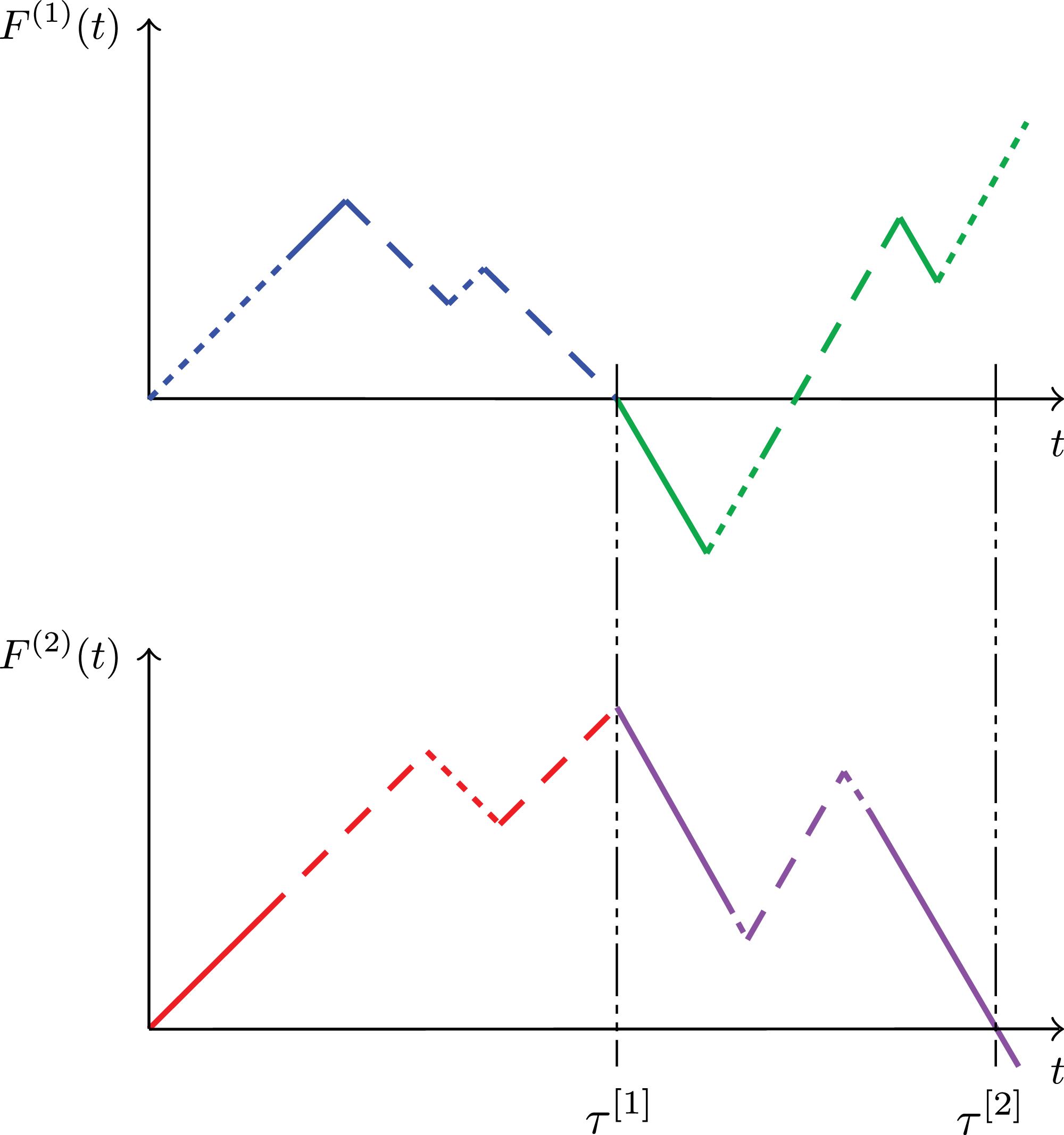
 (F(1),F(2))
 J(k)
J(k) k∈{1,2}
 E(k)
E(k) S(k)
S(k) τ[1]
τ[1]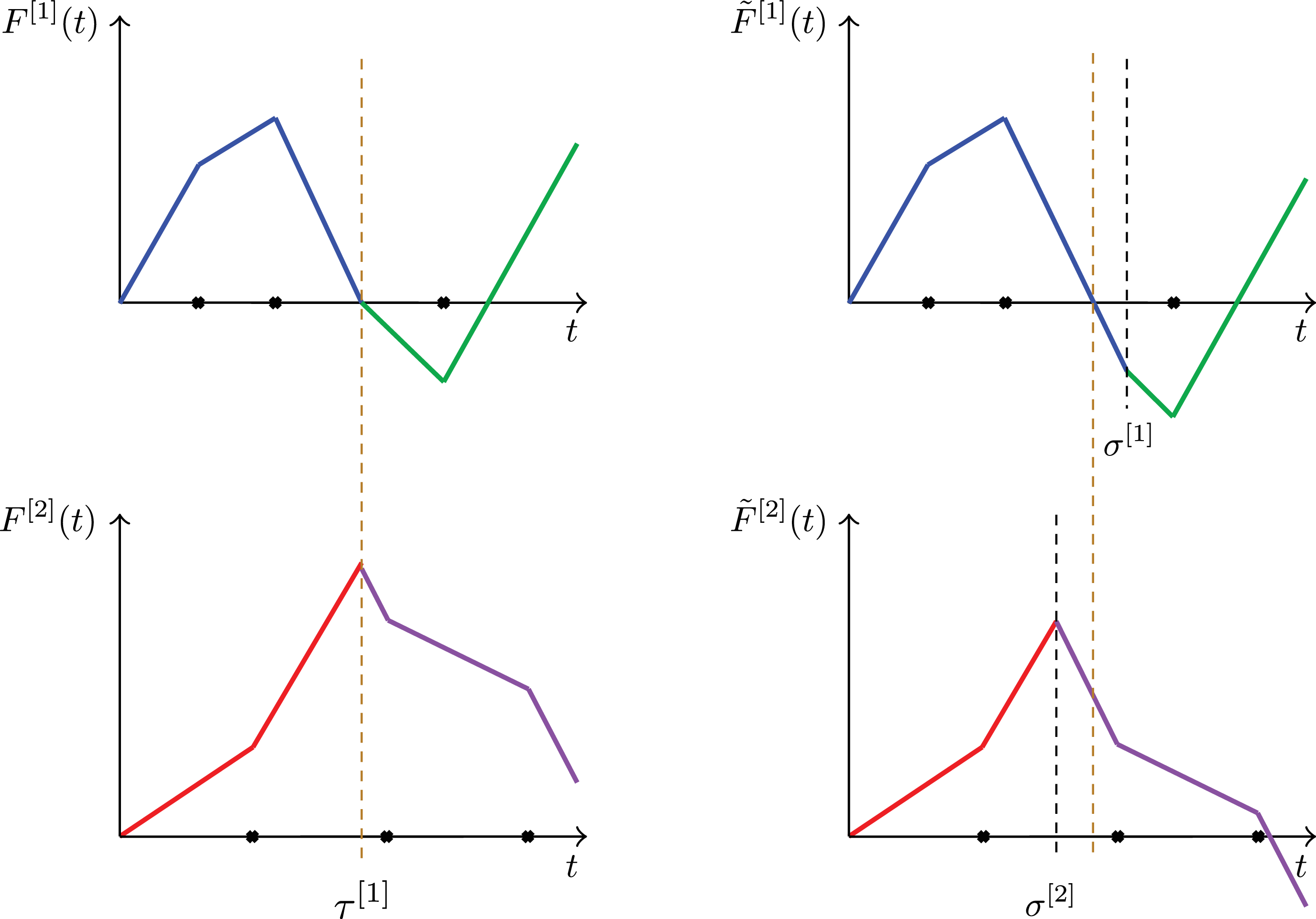
 (F[1],F[2])
 (F~[1],F~[2])
 σ[1]
σ[1] σ[2]
σ[2] J~[1]
J~[1] J~[2]
J~[2] J[1]
J[1] J[2]
J[2]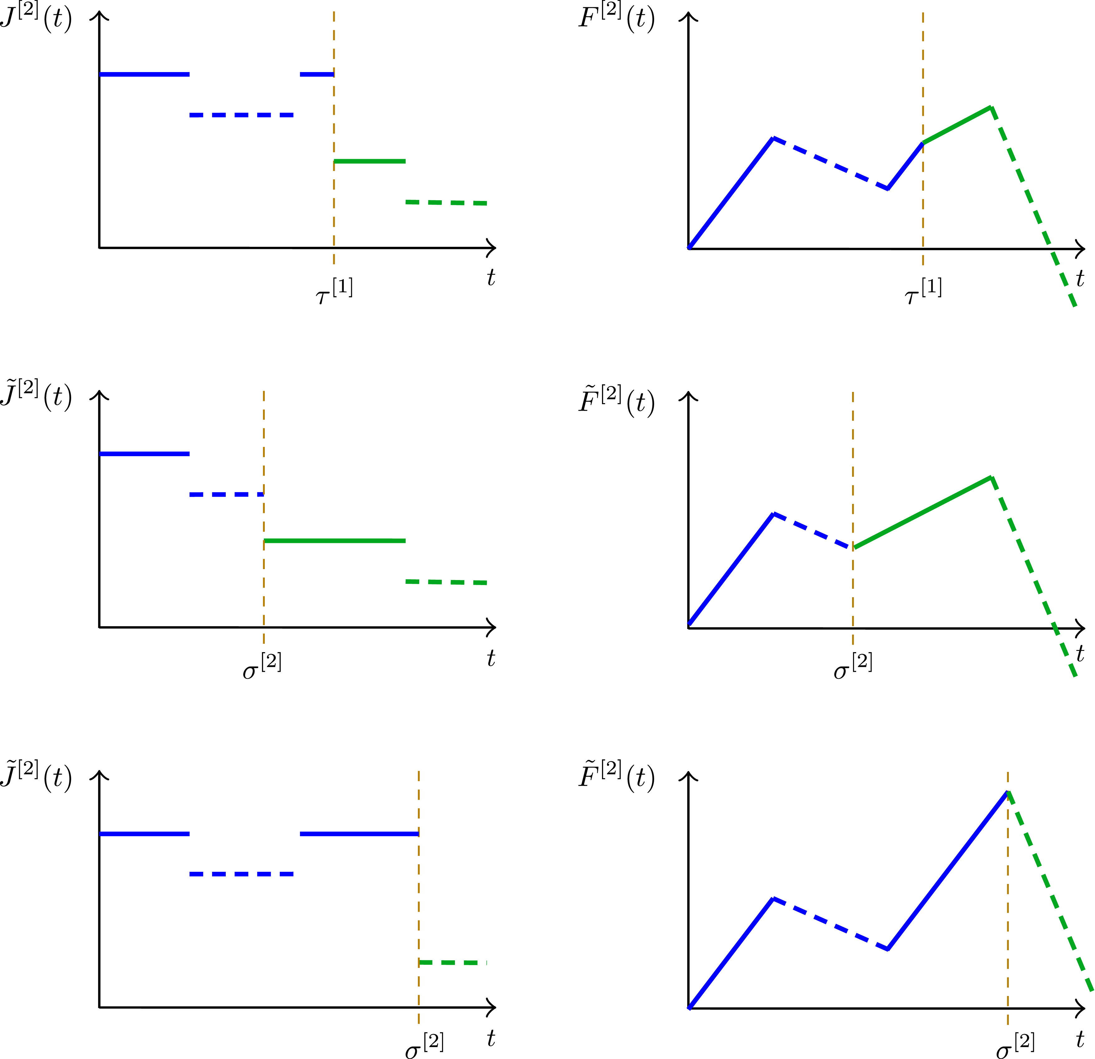
 J[k]
J[k] τ[1]∈[θℓk[k],θℓk+1[k])
 σ(k)′<θℓk[k]
 σ(k)″>θℓk+1[k]
 J[k]
J[k] E[k]
E[k] F~[k]
F~[k] F[k]
F[k]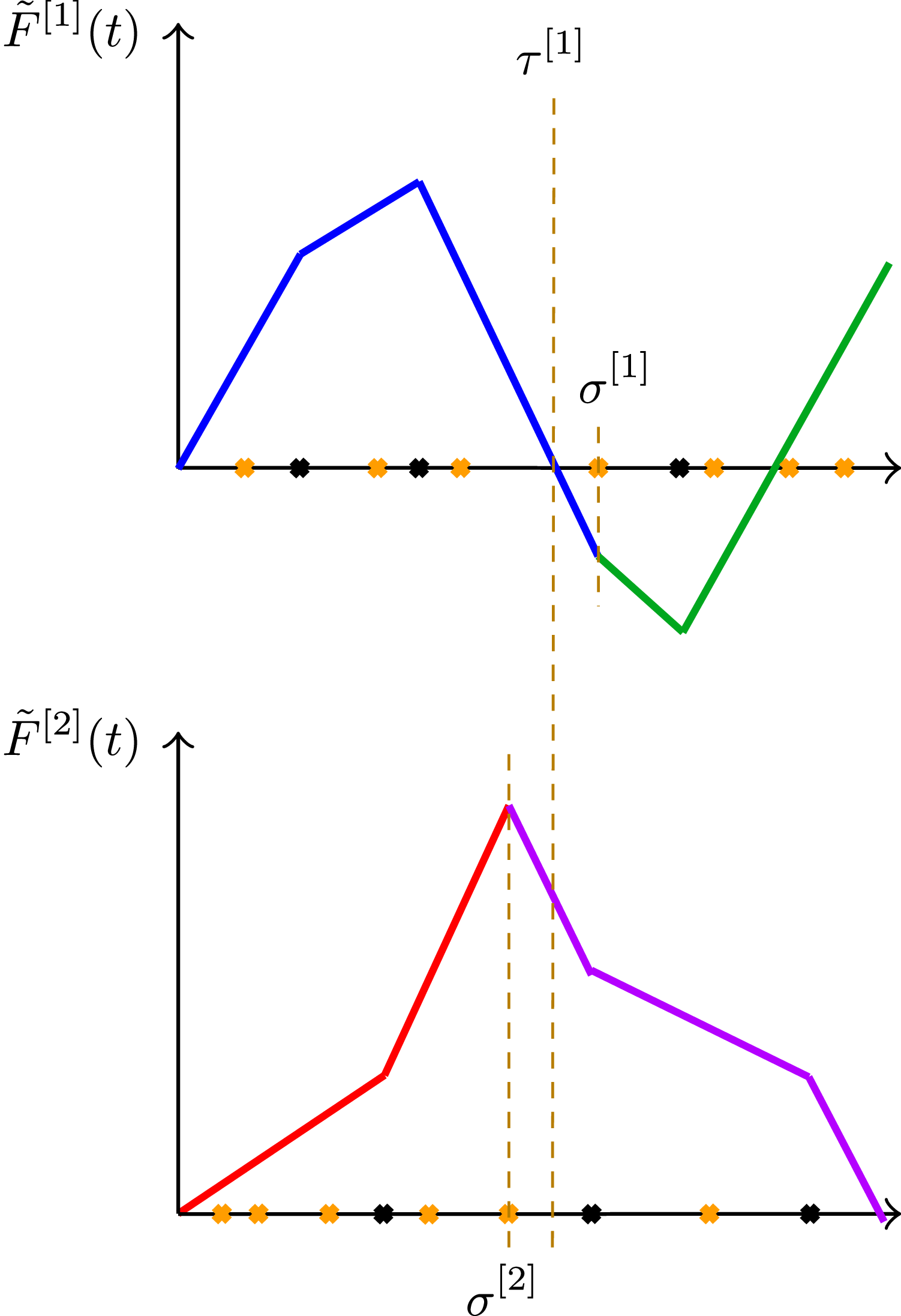
 k∈{1,2}
 Θ[k]
Θ[k] Θ^[k]
Θ^[k] Θ~[k]
Θ~[k] ℓ∗=6
ℓ∗=6 σ[1]=θ~6[1]
 σ[2]=θ~6[2]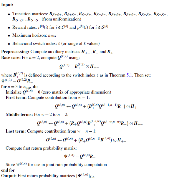
 Ψ(ℓ,n)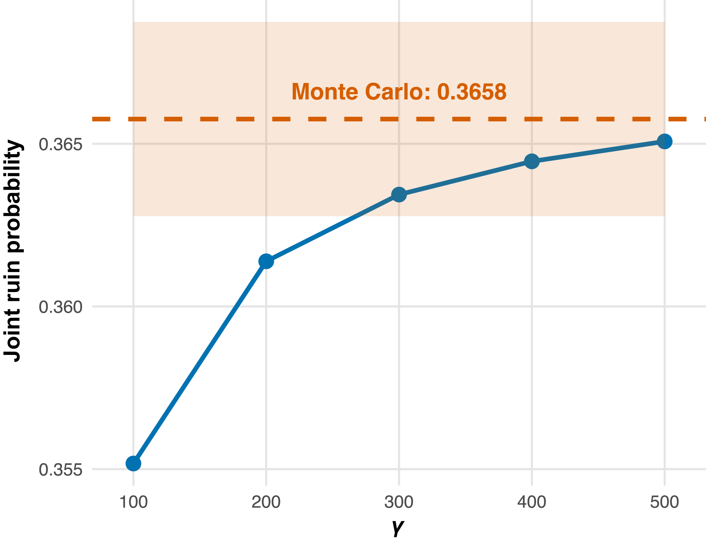
 P(τ[1]≤0.5,τ[2]≤0.6,F[1]=F(1))
 γ
γ γ
γ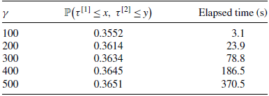
 γ
γ x=0.5
x=0.5 y=0.6
y=0.6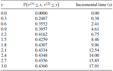
 γ=100
γ=100 x=0.5
x=0.5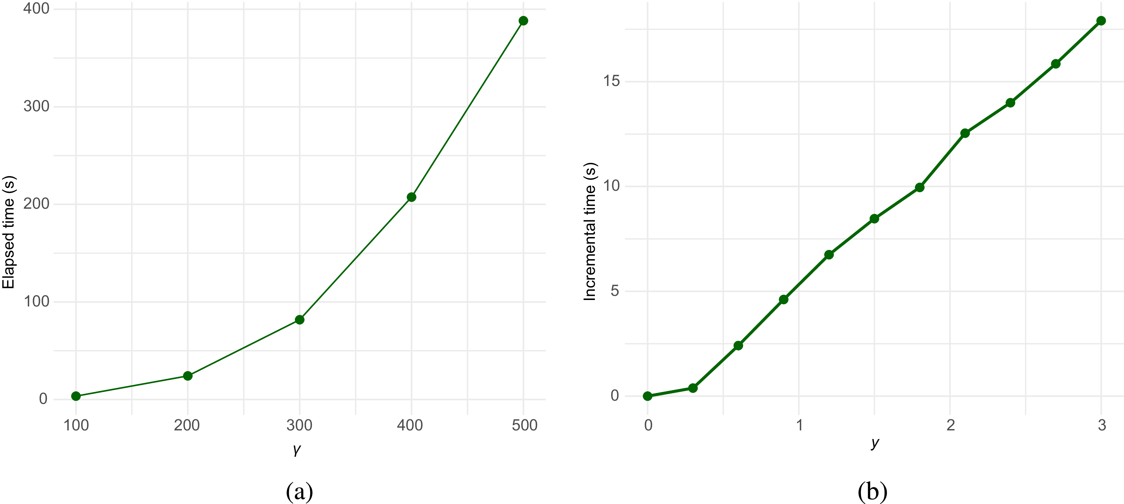
 x=0.5
x=0.5 y=0.6
y=0.6 γ
γ γ=100
γ=100 x=0.5
x=0.5
 G(x,y)=P(τ[1]≤x,τ[2]≤y,F[1]=F(1),F[2]=F(2))
 γ=100
γ=100

