





1. Introduction
Plasma physics has seen significant advances in the ability to simulate nonlinear plasma dynamics from first principles. However, capturing the complex multi-scale dynamics of plasmas, especially in non-equilibrium and strongly coupled regimes, remains challenging (Kushner Reference Kushner2020). One such challenge is the development of collisional operators that capture the macroscopic dynamics in regimes where analytical theory does not exist or is expected to fail, e.g. regimes where the collisional dynamics are mediated by electromagnetic interactions (relativistic temperatures) (Braams & Karney Reference Braams and Karney1987; Pike & Rose Reference Pike and Rose2016) or when assumptions about the predominance of small-angle scattering events break down (strongly coupled regimes) (Baalrud Reference Baalrud2012; Baalrud & Daligault Reference Baalrud and Daligault2014). These regimes occur for example in inertial confinement fusion experiments (Atzeni & Meyer-ter Vehn Reference Atzeni and Meyer-ter Vehn2004), dense astrophysical objects (e.g. white dwarfs, neutron stars, core of gas giants) (Chabrier, Saumon & Potekhin Reference Chabrier, Saumon and Potekhin2006) and in dusty (Merlino & Goree Reference Merlino and Goree2004) and ultracold (Killian et al. Reference Killian, Pattard, Pohl and Rost2007) astrophysical and laboratory plasmas. It is therefore important to design first-principles numerical simulations to probe deviations from the theory and to extract improved models which can serve as the building blocks for future theoretical developments.
For weakly coupled plasmas, where small-angle Coulomb collisions dominate the dynamics, the Fokker–Planck (FP) collision operator is expected to provide a good description of the collisional dynamics (Landau Reference Landau1936; Rosenbluth, MacDonald & Judd Reference Rosenbluth, MacDonald and Judd1957). The operator can be written as (Rosenbluth et al. Reference Rosenbluth, MacDonald and Judd1957)
 \begin{equation} \left (\frac {\partial f}{\partial t}\right )_{FP} = - \boldsymbol{\nabla} _{\boldsymbol{v}}\boldsymbol{\cdot }(\unicode{x1D63C}f) + \frac {1}{2}\boldsymbol{\nabla} _{\boldsymbol{v}}\boldsymbol{\cdot }\left [\boldsymbol{\nabla} _{\boldsymbol{v}}\boldsymbol{\cdot }(\unicode{x1D63F}f)\right ]\!, \end{equation}
where $\boldsymbol{v} \in \mathbb{R}^N$
is the velocity vector in the
$\boldsymbol{v} \in \mathbb{R}^N$
is the velocity vector in the $N$
-dimensional phase space,
$N$
-dimensional phase space, $f(\boldsymbol{v}, t): \mathbb{R}^N \times \mathbb{R} \rightarrow \mathbb{R}$
is the underlying spatially distribution function (for simplicity here we assume that
$f(\boldsymbol{v}, t): \mathbb{R}^N \times \mathbb{R} \rightarrow \mathbb{R}$
is the underlying spatially distribution function (for simplicity here we assume that $f$
does not depend on the position
$f$
does not depend on the position $\boldsymbol{r}$
),
$\boldsymbol{r}$
), $\unicode{x1D63C}(\boldsymbol{v}, t): \mathbb{R}^N \times \mathbb{R} \rightarrow \mathbb{R}^N$
is the advection (drift) vector and
$\unicode{x1D63C}(\boldsymbol{v}, t): \mathbb{R}^N \times \mathbb{R} \rightarrow \mathbb{R}^N$
is the advection (drift) vector and $\unicode{x1D63F}(\boldsymbol{v}, t): \mathbb{R}^N \times \mathbb{R} \rightarrow \mathbb{R}^{N\times N}$
is the diffusion matrix.
$\unicode{x1D63F}(\boldsymbol{v}, t): \mathbb{R}^N \times \mathbb{R} \rightarrow \mathbb{R}^{N\times N}$
is the diffusion matrix.
The FP operator is often coupled with the Vlasov and Maxwell systems of equations to self-consistently model collisional transport and the kinetic evolution of particle distribution functions in phase space (Bell et al. Reference Bell, Robinson, Sherlock, Kingham and Rozmus2006; Tzoufras et al. Reference Tzoufras, Bell, Norreys and Tsung2011; Thomas et al. Reference Thomas, Tzoufras, Robinson, Kingham, Ridgers, Sherlock and Bell2012; Tzoufras et al. Reference Tzoufras, Tableman, Tsung, Mori and Bell2013; Bell & Sherlock Reference Bell and Sherlock2024). Furthermore, it has been shown that other stochastic acceleration processes mediated by turbulence (and not collisional dynamics) can also be studied using this description (Wong et al. Reference Wong, Zhdankin, Uzdensky, Werner and Begelman2020, Reference Wong, Zhdankin, Uzdensky, Werner and Begelman2025; Camporeale et al. Reference Camporeale, Wilkie, Drozdov and Bortnik2022).
Significant theoretical work has been made to determine the mathematical form of the advection and diffusion coefficients that capture the dynamics of interest (Rosenbluth et al. Reference Rosenbluth, MacDonald and Judd1957; Braams & Karney Reference Braams and Karney1987; Reynolds, Fried & Morales Reference Reynolds, Fried and Morales1997). Usually, these efforts result in collisional integrals, which can be costly to compute and to treat analytically. When theory is not available, both numerical and experimental tools have been used to estimate such coefficients, e.g. particle track information from numerical simulations is commonly used to infer the coefficients for a set-up of interest (Hockney Reference Hockney1971; Matsuda & Okuda Reference Matsuda and Okuda1975; Wong et al. Reference Wong, Zhdankin, Uzdensky, Werner and Begelman2020, Reference Wong, Zhdankin, Uzdensky, Werner and Begelman2025). While particle tracks provide all the required information to estimate the coefficients, it is often unfeasible to store and post-process all the necessary data for large-scale simulations and broad parameter scans. Furthermore, to accurately estimate the coefficients (at run time) and, therefore, avoid storing the full tracks, one needs to a priori have an estimate of all the acceleration (forces) time scales involved (not only collisions). In particular, one must guarantee that the time step over which velocity change statistics are computed fulfils the Markovian assumption underpinning the FP equation.
In this work, we propose a general-purpose framework to learn collision operators from phase space data (in this paper, obtained from kinetic numerical simulations) by rewriting the problem as an optimisation task, which we tackle using a differentiable kinetic simulator and gradient-based minimisation methods. The simulator evolves phase space distributions using a differentiable FP solver, where the advection and diffusion tensors are learned from data. By making use solely of phase space data, we greatly reduce the memory requirements associated with storing particle tracks. Furthermore, the differentiable simulator allows us to extract operators that accurately capture the long-term dynamics without prior knowledge of the involved time scales. The technique is general and can be used with other sets of phase space information, e.g. from experimental (Bergeson et al. Reference Bergeson, Schlitters, Miller, Farley, Sieverts, Murillo and Haack2025) or observational (Camporeale et al. Reference Camporeale, Wilkie, Drozdov and Bortnik2022) data, and the simulator can be extended to include different collision operator forms, external fields or other options deemed relevant for the problem under study.
As a first test case, we use these tools to extract the collision operator for an electromagnetic particle-in-cell (PIC) code (Birdsall & Langdon Reference Birdsall and Langdon2018), which evolves the self-consistent fields of finite-size particles, and compare the results against theory originally proposed by Langdon (Reference Langdon and Birdsall1970) and Langdon & Birdsall (Reference Langdon and Birdsall1970), and against coefficients derived from particle tracks. This is a good test bench since theoretical predictions assume that a FP-type collision operator correctly captures the self-consistent collisional dynamics of the PIC algorithm. We note that the collision operator we aim to extract is not explicitly solved by the PIC algorithm, e.g. via a Monte Carlo module (Takizuka & Abe Reference Takizuka and Abe1977) or a grid-based Langevin operator (Manheimer, Lampe & Joyce Reference Manheimer, Lampe and Joyce1997). The learned operator is instead a consequence of the self-consistent interactions between the finite-size particles and the generated fields in a regime where small-angle scattering events are expected to dominate.
This paper is structured as follows. In §§ 1.1 and 1.2 we review the underpinning theoretical and numerical results. In § 2 we describe the methods deployed in this paper to learn collision operators. In § 3 we present the main results for the collision operator learned for plasmas of finite-size particles. Finally, in § 4 we state the conclusions and describe directions for future work.
1.1. The PIC collision operator
The PIC algorithm (Birdsall & Langdon Reference Birdsall and Langdon2018) solves the Klimontovich equation (Klimontovich Reference Klimontovich1967) for finite-size particles,Footnote 1 coupled with the Maxwell system of equations (or a subset) to self-consistently model the fields generated by the movement of the particles and advance their position over time. Since particles have a finite size, the electrostatic force between two particles is reduced at short distances (comparable to the particle radius), which significantly reduces the short-range collisional interactions compared with point-like particles; we note that the long-range interactions are correctly captured. Hence, the effective Coulomb collision operator for PIC-simulated plasmas is modified relative to that of real plasmas.
Theoretical work on the collision operator for plasmas composed of finite-size particles was originally made by Langdon (Reference Langdon and Birdsall1970), Langdon & Birdsall (Reference Langdon and Birdsall1970) and Okuda & Birdsall (Reference Okuda and Birdsall1970). Langdon (Reference Langdon and Birdsall1970) derived the first description of a FP collision operator for electrostatic PIC simulations, which includes the effect of aliasing due to the finite grid size, discrete time step and shape function, among others. More recently, Touati et al. (Reference Touati, Codur, Tsung, Decyk, Mori and Silva2022) thoroughly re-derived these results and extended the description to include the effect of varying macroparticle weights.
Several numerical experiments were conducted to complement and verify some predictions using electrostatic PIC codes. Hockney (Reference Hockney1971) empirically studied collisional relaxation rates and inferred a scaling law for two-dimensional (2-D) thermalisation times for the nearest grid point (zeroth-order interpolation) and cloud-in-cell (CIC, first-order interpolation) shape functions. Matsuda & Okuda (Reference Matsuda and Okuda1975) performed direct comparisons between the predicted advection for Gaussian-shaped particles moving at $v=v_{th} = \sqrt {k_B T/m}$
(where
$v=v_{th} = \sqrt {k_B T/m}$
(where $k_B$
is the Boltzmann constant,
$k_B$
is the Boltzmann constant, $T$
the species temperature, and
$T$
the species temperature, and $m$
the species mass) and diffusion for particles at rest
$m$
the species mass) and diffusion for particles at rest $v=0$
for both 2-D and 3-D simulations. They found that for ions the theoretical predictions were accurate within a
$v=0$
for both 2-D and 3-D simulations. They found that for ions the theoretical predictions were accurate within a $20\,\%$
error, while for electrons the predictions could deviate from the result up to a factor of
$20\,\%$
error, while for electrons the predictions could deviate from the result up to a factor of $200\,\%$
. They also demonstrated that, when imposing a strong external magnetic field, the collisionality of the simulated plasma decreases significantly if the gyroradius is smaller than the particle size. More recently, Gatsonis & Spirkin (Reference Gatsonis and Spirkin2009) and Averkin & Gatsonis (Reference Averkin and Gatsonis2018) studied deflection and slow-down times in 3-D PIC codes with unstructured Delaunay–Voronoi grids, and Jubin et al. (Reference Jubin, Powis, Villafana, Sydorenko, Rauf, Khrabrov, Sarwar and Kaganovich2024) studied numerical relaxation rates for 2-D low-temperature plasma set-ups using CIC shape functions while proposing mitigation strategies to reduce undesired thermalisation effects due to finite-size particle collisions. Finally, Park, Moore & Baalrud (Reference Park, Moore and Baalrud2025) complemented the work of Jubin et al. (Reference Jubin, Powis, Villafana, Sydorenko, Rauf, Khrabrov, Sarwar and Kaganovich2024) by thoroughly exploring 1-D, 2-D and 3-D scenarios.
$200\,\%$
. They also demonstrated that, when imposing a strong external magnetic field, the collisionality of the simulated plasma decreases significantly if the gyroradius is smaller than the particle size. More recently, Gatsonis & Spirkin (Reference Gatsonis and Spirkin2009) and Averkin & Gatsonis (Reference Averkin and Gatsonis2018) studied deflection and slow-down times in 3-D PIC codes with unstructured Delaunay–Voronoi grids, and Jubin et al. (Reference Jubin, Powis, Villafana, Sydorenko, Rauf, Khrabrov, Sarwar and Kaganovich2024) studied numerical relaxation rates for 2-D low-temperature plasma set-ups using CIC shape functions while proposing mitigation strategies to reduce undesired thermalisation effects due to finite-size particle collisions. Finally, Park, Moore & Baalrud (Reference Park, Moore and Baalrud2025) complemented the work of Jubin et al. (Reference Jubin, Powis, Villafana, Sydorenko, Rauf, Khrabrov, Sarwar and Kaganovich2024) by thoroughly exploring 1-D, 2-D and 3-D scenarios.
In this work, we extend these previous results by providing a thorough comparison between predicted and measured advection and diffusion coefficients for a broad range of particle velocities ( $v_{x,y}/v_{th} \in [0, 5])$
and simulation parameters (shape functions, grid resolution, particles per cell, thermal velocity). Furthermore, we conduct these tests for the first time using an electromagnetic PIC code (Fonseca et al. Reference Fonseca2002). We note that the theory of collisions in plasmas is based purely on electrostatic interactions, so this work provides an important first step on possible modifications of the collisional operators when including self-consistent electromagnetic interactions. For all scenarios, we consider the 2-D version of OSIRIS (Fonseca et al. Reference Fonseca2002) that utilises a finite-difference time-domain (FDTD) Yee solver (Yee Reference Yee1966), and a plasma consisting of a single mobile electron species moving over a uniform neutralising ion background.
$v_{x,y}/v_{th} \in [0, 5])$
and simulation parameters (shape functions, grid resolution, particles per cell, thermal velocity). Furthermore, we conduct these tests for the first time using an electromagnetic PIC code (Fonseca et al. Reference Fonseca2002). We note that the theory of collisions in plasmas is based purely on electrostatic interactions, so this work provides an important first step on possible modifications of the collisional operators when including self-consistent electromagnetic interactions. For all scenarios, we consider the 2-D version of OSIRIS (Fonseca et al. Reference Fonseca2002) that utilises a finite-difference time-domain (FDTD) Yee solver (Yee Reference Yee1966), and a plasma consisting of a single mobile electron species moving over a uniform neutralising ion background.
Under these conditions, and when neglecting the effect of temporal and spatial aliasing, the theoretical advection $\unicode{x1D63C}(\boldsymbol{v})$
and diffusion
$\unicode{x1D63C}(\boldsymbol{v})$
and diffusion $\unicode{x1D63F}(\boldsymbol{v})$
operators for the finite-size e–e collisions are given (in S.I. units) by (cf. derivation in Supplemental Material S1)
$\unicode{x1D63F}(\boldsymbol{v})$
operators for the finite-size e–e collisions are given (in S.I. units) by (cf. derivation in Supplemental Material S1)
 \begin{equation} \unicode{x1D63C}(\boldsymbol{v}) = \unicode{x1D63C}^{(1)}(\boldsymbol{v}) + \unicode{x1D63C}^{(2)}(\boldsymbol{v}) ,\end{equation}
 \begin{equation} \unicode{x1D63C}^{(1)}(\boldsymbol{v}) = -\frac {\omega _{p} v_{th}}{N_{Dmac} 2^{5/2} \pi ^{3/2}} \int _{\mathbb{R}^2} \mathbf{d}\boldsymbol{\tilde{k}} \frac {S_\rho ^m(\boldsymbol{\tilde{k}})^4}{\left | \epsilon (\boldsymbol{\tilde{k}} \boldsymbol{\cdot } \boldsymbol{\tilde{v}}, \boldsymbol{\tilde{k}}) \right |^2 {\tilde{k}}_s^4} \frac {\boldsymbol{\tilde{k}_s}(\boldsymbol{\tilde{k}_s} \boldsymbol{\cdot } \boldsymbol{\tilde{k}})(\boldsymbol{\tilde{k}} \boldsymbol{\cdot } \boldsymbol{\tilde{v}})}{{\tilde{k}}^3} e^{-(\boldsymbol{\tilde{k}} \boldsymbol{\cdot } \boldsymbol{\tilde{v}})^2 / 2{\tilde{k}}^2} ,\end{equation}
 \begin{equation} \unicode{x1D63C}^{(2)}(\boldsymbol{v}) = \frac {1}{2v_{th}}\boldsymbol{\nabla} _{\boldsymbol{\tilde{v}}} \boldsymbol{\cdot } \unicode{x1D63F}(\boldsymbol{v}) ,\end{equation}
 \begin{equation} \unicode{x1D63F}(\boldsymbol{v}) = \frac {\omega _{p} v_{th}^2}{N_{Dmac} 2^{3/2} \pi ^{3/2}} \int _{\mathbb{R}^2} \mathbf{d}\boldsymbol{\tilde{k}} \frac {S_\rho ^m(\boldsymbol{\tilde{k}})^4}{\left | \epsilon (\boldsymbol{\tilde{k}} \boldsymbol{\cdot } \boldsymbol{\tilde{v}}, \boldsymbol{\tilde{k}})\right |^2 \tilde{{k}}_s^4} \frac {(\boldsymbol{\tilde{k}}_s \otimes \boldsymbol{\tilde{k}}_s)}{{\tilde{k}}} e^{-(\boldsymbol{\tilde{k}} \boldsymbol{\cdot } \boldsymbol{\tilde{v}})^2 / 2{\tilde{k}}^2} ,\end{equation}
where the pre-factor constants correspond to the electron plasma frequency $\omega _p = \sqrt {n_e e^2 /\varepsilon _0 m_e}$
(with
$\omega _p = \sqrt {n_e e^2 /\varepsilon _0 m_e}$
(with $n_e$
being the electron number density,
$n_e$
being the electron number density, $e$
the electron charge,
$e$
the electron charge, $\varepsilon _0$
the vacuum permittivity and
$\varepsilon _0$
the vacuum permittivity and $m_e$
electron mass), and the number of macroparticles per Debye square
$m_e$
electron mass), and the number of macroparticles per Debye square $N_{Dmac} = n_{mac}\lambda _D^2$
where
$N_{Dmac} = n_{mac}\lambda _D^2$
where $\lambda _D = v_{th}/\omega _p$
is the electron Debye length and
$\lambda _D = v_{th}/\omega _p$
is the electron Debye length and $n_{mac}=N_{ppc}/(\varDelta _x\varDelta _y)$
is the macroparticle number density (with
$n_{mac}=N_{ppc}/(\varDelta _x\varDelta _y)$
is the macroparticle number density (with $N_{ppc}$
being the number of particles per cell and
$N_{ppc}$
being the number of particles per cell and $\varDelta _{x,y}$
the grid resolution). The integral is defined over
$\varDelta _{x,y}$
the grid resolution). The integral is defined over $\mathbb{R}^2$
and all vector quantities have two directions (e.g.
$\mathbb{R}^2$
and all vector quantities have two directions (e.g. $\boldsymbol{\tilde{v}} = (\tilde{v}_x, \tilde{v}_y)$
,
$\boldsymbol{\tilde{v}} = (\tilde{v}_x, \tilde{v}_y)$
, $\mathbf{d}\boldsymbol{\tilde{k}} = \mathrm{d}\tilde{k}_x\mathrm{d}\tilde{k}_y$
,);
$\mathbf{d}\boldsymbol{\tilde{k}} = \mathrm{d}\tilde{k}_x\mathrm{d}\tilde{k}_y$
,); $\boldsymbol{\tilde{v}} = \boldsymbol{v}/v_{th}$
is the particle velocity normalised to the thermal velocity,
$\boldsymbol{\tilde{v}} = \boldsymbol{v}/v_{th}$
is the particle velocity normalised to the thermal velocity, $\boldsymbol{\tilde{k}} = \boldsymbol{k}\lambda _D$
is the wave vector normalised by the inverse of the electron Debye length and
$\boldsymbol{\tilde{k}} = \boldsymbol{k}\lambda _D$
is the wave vector normalised by the inverse of the electron Debye length and $\boldsymbol{\tilde{k}_s} = \boldsymbol{k_s} \lambda _D$
is a dimensionless vector associated with the FDTD field solver used where
$\boldsymbol{\tilde{k}_s} = \boldsymbol{k_s} \lambda _D$
is a dimensionless vector associated with the FDTD field solver used where $\boldsymbol{k}_s = (k_x \mathrm{sinc}(k_x\varDelta _x/2), k_y\mathrm{sinc}(k_y\varDelta _y/2))$
with
$\boldsymbol{k}_s = (k_x \mathrm{sinc}(k_x\varDelta _x/2), k_y\mathrm{sinc}(k_y\varDelta _y/2))$
with $\mathrm{sinc}(x) = \sin (x)/x$
. Finally,
$\mathrm{sinc}(x) = \sin (x)/x$
. Finally, $S_\rho ^m(\boldsymbol{\tilde{k}}) = \mathrm{sinc}({\tilde{k}}_x \varDelta _x/2\lambda _D)^{m+1}\mathrm{sinc}({\tilde{k}}_y \varDelta _y/2\lambda _D)^{m+1}$
is the charge deposition shape function of order
$S_\rho ^m(\boldsymbol{\tilde{k}}) = \mathrm{sinc}({\tilde{k}}_x \varDelta _x/2\lambda _D)^{m+1}\mathrm{sinc}({\tilde{k}}_y \varDelta _y/2\lambda _D)^{m+1}$
is the charge deposition shape function of order $m$
, and
$m$
, and $\epsilon$
the dielectric function defined as (cf. derivation in Supplemental Material S1)
$\epsilon$
the dielectric function defined as (cf. derivation in Supplemental Material S1)
 \begin{equation} \epsilon (\boldsymbol{\tilde{k}} \boldsymbol{\cdot } \boldsymbol{\tilde{v}}, \boldsymbol{\tilde{k}}) = 1 - \frac {S_\rho ^m(\boldsymbol{\tilde{k}})^2 (\boldsymbol{\tilde{k}}_s \boldsymbol{\cdot } \boldsymbol{\tilde{k}})}{2 {\tilde{k}}_s^2 {\tilde{k}}^2} Z'\left ( \frac {\boldsymbol{\tilde{k}} \boldsymbol{\cdot } \boldsymbol{\tilde{v}}}{\sqrt {2}{\tilde{k}}} \right )\! ,\end{equation}
where $Z'(\xi ) = \pi ^{-1/2} \int _{\mathbb{R}} \text{d}t \,e^{-t^2}/(\xi - t)^2$
is the first derivative of the plasma dispersion function (Fried & Conte Reference Fried and Conte1961). A more in-depth discussion regarding the derivation of the advection and diffusion coefficients (based on the more general form of the PIC collision operator derived by Touati et al. (Reference Touati, Codur, Tsung, Decyk, Mori and Silva2022)) is provided in Supplementary Material S1.
$Z'(\xi ) = \pi ^{-1/2} \int _{\mathbb{R}} \text{d}t \,e^{-t^2}/(\xi - t)^2$
is the first derivative of the plasma dispersion function (Fried & Conte Reference Fried and Conte1961). A more in-depth discussion regarding the derivation of the advection and diffusion coefficients (based on the more general form of the PIC collision operator derived by Touati et al. (Reference Touati, Codur, Tsung, Decyk, Mori and Silva2022)) is provided in Supplementary Material S1.
1.2. Related machine learning work
The machine learning community has proposed several approaches to learning operators that recover observed dynamical data (a type of inverse problem). Common neural network (NN) based approaches include neural operators such as deep operator networks (Lu, Jin & Karniadakis Reference Lu, Jin and Karniadakis2019) and Fourier neural operators (Li et al. Reference Li, Kovachki, Azizzadenesheli, Liu, Bhattacharya, Stuart and Anandkumar2020), among many others (Kovachki et al. Reference Kovachki, Li, Liu, Azizzadenesheli, Bhattacharya, Stuart and Anandkumar2023) designed to learn mappings between function spaces. While these approaches are extremely flexible, since the operator form is not hard constrained, they require substantial amounts of training data to obtain an accurate general operator. Furthermore, the learned operator is, by construction, not interpretable. On the other hand, physics-informed NNs (PINNs) (Raissi, Perdikaris & Karniadakis Reference Raissi, Perdikaris and Karniadakis2019) or discrete grid-based alternatives (Karnakov, Litvinov & Koumoutsakos Reference Karnakov, Litvinov and Koumoutsakos2022), can also be used to extract operators at a significantly reduced data cost. However, they require the underlying form of the operator to be defined a priori, and the full solution of the differential equation must also be learned during the fitting process. A middle ground between traditional numerical solvers and data-driven methods is found in universal differentiable equations (UDEs) (Rackauckas et al. Reference Rackauckas, Ma, Martensen, Warner, Zubov, Supekar, Skinner, Ramadhan and Edelman2020), where learnable models (e.g. NNs) are integrated within a prescribed differentiable simulator. Therefore, UDEs combine the benefits of previous extensive research on traditional numerical solvers with the flexibility of data-driven approaches. This is an important combination for problems where we want to strongly enforce known physical biases and numerical constraints, and are not interested in creating a surrogate model for the differential equation solution (since the cost of integrating the dynamics with the simulator is not significant). Our work belongs to this family of algorithms: we combine a differentiable FP solver with learnable advection/diffusion operators. Interpretable symbolic regression methods can also be used for this task (Brunton, Proctor & Kutz Reference Brunton, Proctor and Kutz2016; Rudy et al. Reference Rudy, Brunton, Proctor and Kutz2017; Gurevich et al. Reference Gurevich, Golden, Reinbold and Grigoriev2024). However, to correctly recover the operator, its expression must be a linear combination of the library of pre-defined terms. This is a problem in situations where we do not have an intuition on what the underlying form of the operator is, or how its coefficients should be parameterised, since there exist infinite possible combinations of input variables that can be added to the library.
The majority of recent work at the intersection of machine learning and collision operators for plasma physics simulations has focused on reducing the associated computational cost of evaluating the collision operator using surrogate models. For example, surrogate models were trained for the Landau–Fokker–Planck (Miller et al. Reference Miller, Churchill, Dener, Chang, Munson and Hager2021; Lee et al. Reference Lee, Jang and Hwang2023; Noh, Lee & Yoon Reference Noh, Lee and Yoon2025), Rosenbluth–Fokker–Planck (Chung et al. Reference Chung, Fei, Gorji and Jenny2023) and Boltzmann (Holloway, Wood & Alekseenko Reference Holloway, Wood and Alekseenko2021; Xiao & Frank Reference Xiao and Frank2021, Reference Xiao and Frank2023; Miller et al. Reference Miller, Roberts, Bond and Cyr2022; Lee et al. Reference Lee, Schotthöfer, Xiao, Krumscheid and Frank2024, Reference Lee, Jung, Lim and Hwang2025) collision operators. Unlike our work, the underlying simulation data used for training all these models were explicitly solving the prescribed collision operator. The goal of these approaches was to reduce the computational cost of evaluating the operator, not to inform the discovery of a new model (the goal of the present work).
PINNs have also been extensively used to model equations that contain FP-type operators. This includes works on the Vlasov–Fokker–Planck (Hwang et al. Reference Hwang, Jang, Jo and Lee2020), the Vlasov–Poisson–Fokker–Planck (Lee, Jang & Hwang Reference Lee, Jang and Hwang2021), the Landau–Fokker–Planck (Chung et al. Reference Chung, Fei, Gorji and Jenny2023) and the FP (Xu et al. Reference Xu, Zhang, Li, Zhou, Liu and Kurths2020; Chen et al. Reference Chen, Yang, Duan and Karniadakis2021; Zhai, Dobson & Li Reference Zhai, Dobson and Li2022; Zhang & Yuen Reference Zhang and Yuen2022; Wang et al. Reference Wang, Hu, Kawaguchi, Zhang and Karniadakis2025) equations. Similarly, PINNs have been used to solve the Boltzmann equation for weakly ionised plasmas (Kawaguchi & Murakami Reference Kawaguchi and Murakami2022; Zhong, Wu & Wang Reference Zhong, Wu and Wang2022), the simplified Boltzmann-Bhatnagar-Gross-Krook equation (Lou, Meng & Karniadakis Reference Lou, Meng and Karniadakis2021; Li et al. Reference Li, Wang, Liu, Wang and Dong2024; Oh et al. Reference Oh, Cho, Yun, Park and Hong2025) and relativistic FP equations describing the runaway electron dynamics in magnetic confinement fusion devices (McDevitt Reference McDevitt2023; McDevitt et al. Reference McDevitt, Arnaud and Tang2025a , Reference McDevitt, Arnaud and Tangb ).
We emphasise that, with the exception of Chen et al. (Reference Chen, Yang, Duan and Karniadakis2021), all previous examples focus on solving the equation of interest (a forward problem) using a prescribed collision operator (with fixed, non-learnable coefficients) rather than on extracting a new operator from the observed dynamics (an inverse problem), as we aim in this paper. While Chen et al. (Reference Chen, Yang, Duan and Karniadakis2021) proposed using PINNs to simultaneously address the forward and inverse problems, the simulation data in that work were generated by explicitly solving the equation with the learned collision operator, whereas in our work the data are obtained from first-principles simulations, that capture the electromagnetic interactions between particles self-consistently.
An exception to this line of research is the work of Camporeale et al. (Reference Camporeale, Wilkie, Drozdov and Bortnik2022), who used PINNs to learn FP operators that capture the observed electron dynamics in the Earth’s radiation belts. The underlying motivation and method are the same as ours, with the exception that we use a differentiable simulator to integrate the dynamics. We believe our approach to be more advantageous for our case study since we can generate as much kinetic simulation data as required, and the differentiable simulator allows us to quickly extract the collision operator without having to train a PINN, as in Camporeale et al. (Reference Camporeale, Wilkie, Drozdov and Bortnik2022). Additionally, in this work, we highlight the reason why the PINNs in Camporeale et al. (Reference Camporeale, Wilkie, Drozdov and Bortnik2022) do not find a unique solution to the advection/diffusion operators and propose an approach to mitigate this problem.
Another very promising related work is that of Zhao & Lei (Reference Zhao and Lei2025) and Zhao et al. (Reference Zhao, Burby, Christlieb and Lei2025), which recently proposed an approach to learn collision operators from molecular dynamics (MD) data. Similarly to our work, they infer a collision operator from kinetic data, with the operator written in its integral formulation. They demonstrate the capability of this formulation to accurately capture the results of MD simulations for both strongly coupled and weakly correlated plasmas initially outside thermal equilibrium. Unlike our approach here, they still use particle tracks during training while we learn directly from phase space data. Our approach, as previously explained, is more efficient in terms of storage requirements and can be more easily generalisable to other datasets. Furthermore, while their approach minimises the prediction error over one time step, ours optimises for long-term stability since we use a differentiable simulator to integrate the dynamics over multiple time steps. Lastly, while the formulation of the operator proposed in Zhao et al. (Reference Zhao, Burby, Christlieb and Lei2025) is tuned specifically for collisional dynamics, the FP description proposed in this work is applicable to other processes.
Differentiable simulators have been previously used in plasma physics to tackle distinct problems. Examples include the discovery of long-lived plasma wave packets (Joglekar & Thomas Reference Joglekar and Thomas2022), learning a fluid closure for nonlinear Landau damping (Joglekar & Thomas Reference Joglekar and Thomas2023), mitigating laser–plasma instabilities (Joglekar Reference Joglekar2024) and simulating the kinetic dynamics of a 1-D plasma with arbitrary degrees of collisionality (Carvalho, Ferreira & Silva Reference Carvalho, Ferreira and Silva2024). While it can be argued that a collisional operator was being learned in Carvalho et al. (Reference Carvalho, Ferreira and Silva2024), the main motivation of the work was reducing the run time of the simulator. Furthermore, the graph NN model used only captures collisions between a reduced number of neighbouring electrons and does not provide an interpretable description as presented in this work.
2. Methods
Our aim is to extract advection and diffusion operators that are capable of reproducing the collisional dynamics of a plasma composed of finite-size particles. Based on the generated simulated data, we will use two different methods to estimate the coefficients. The first method makes use of particle tracks and is the standard approach from previous literature (Hockney Reference Hockney1971; Matsuda & Okuda Reference Matsuda and Okuda1975). The second is the novel contribution of the work, and consists of using only the distribution function (phase space) evolution of subpopulations to estimate the operator using a differentiable simulator framework. We will examine the benefits/tradeoffs between the two approaches later in this work.
2.1. Particle-in-cell simulations
Throughout this work, we perform 2-D simulations using the electromagnetic PIC code OSIRIS (Fonseca et al. Reference Fonseca2002). We consider a single mobile electron species moving over a fixed uniform ion background inside a periodic box. In these simulations, only electron–electron collisions are captured. The initial electron velocities are sampled from a thermal distribution with zero net velocity and standard deviation $v_{th}$
in all directions, and the simulation window is set to
$v_{th}$
in all directions, and the simulation window is set to $10^3\lambda _D\times 10^3\lambda _D$
. For all scenarios, we use a charge-conserving current deposition scheme (Esirkepov Reference Esirkepov2001), a second-order FDTD electromagnetic field solver (Yee Reference Yee1966) and the standard Boris pusher (Boris & Shanny Reference Boris and Shanny1972) to advance particle momenta and position.
$10^3\lambda _D\times 10^3\lambda _D$
. For all scenarios, we use a charge-conserving current deposition scheme (Esirkepov Reference Esirkepov2001), a second-order FDTD electromagnetic field solver (Yee Reference Yee1966) and the standard Boris pusher (Boris & Shanny Reference Boris and Shanny1972) to advance particle momenta and position.
To generate a dataset of simulations with different advection and diffusion operators, we vary four parameters: the number of particles per cell ( $N_{ppc}$
), the current deposition shape function (
$N_{ppc}$
), the current deposition shape function ( $S_J^m$
, where
$S_J^m$
, where $m$
is the interpolation order), the ratio of the grid-resolution over the electron Debye length (
$m$
is the interpolation order), the ratio of the grid-resolution over the electron Debye length ( $\varDelta _x/\lambda _D$
=
$\varDelta _x/\lambda _D$
= $\varDelta _y/\lambda _D$
) and the electron thermal velocity (
$\varDelta _y/\lambda _D$
) and the electron thermal velocity ( $v_{th}/c$
). In total, we performed approximately 100 simulations corresponding to different parameter combinations and preserved a subset of approximately 75 simulations for which no significant PIC heating was observed.Footnote
2
The detailed list of simulation parameters used and the heating tests performed is provided in Supplementary Material S2.
$v_{th}/c$
). In total, we performed approximately 100 simulations corresponding to different parameter combinations and preserved a subset of approximately 75 simulations for which no significant PIC heating was observed.Footnote
2
The detailed list of simulation parameters used and the heating tests performed is provided in Supplementary Material S2.
For each simulation, we stored the raw data of all macroparticles (approximately $10^6{-}10^7$
macroparticles depending on the numerical parameters, we store both their position and momenta) at equally spaced time intervals to collect a minimum of 100 snapshots over the full simulation. This information is used to construct the phase space information of different subpopulations in post-processing, as described in Supplementary Material S3. We note that we only store the data of all macroparticles to be able to compare the operators recovered from the two methods: from macroparticle particle tracks (i.e. macroparticle position and momenta history), and from the phase space evolution of subpopulations. In future works, this memory-intensive step will not be required.
$10^6{-}10^7$
macroparticles depending on the numerical parameters, we store both their position and momenta) at equally spaced time intervals to collect a minimum of 100 snapshots over the full simulation. This information is used to construct the phase space information of different subpopulations in post-processing, as described in Supplementary Material S3. We note that we only store the data of all macroparticles to be able to compare the operators recovered from the two methods: from macroparticle particle tracks (i.e. macroparticle position and momenta history), and from the phase space evolution of subpopulations. In future works, this memory-intensive step will not be required.
2.2. Advection–diffusion coefficients from particle tracks
The advection and diffusion coefficients for particles moving at a specific velocity $\boldsymbol{v}$
can be estimated by tracking the rate of the average velocity drift and spread over time
$\boldsymbol{v}$
can be estimated by tracking the rate of the average velocity drift and spread over time


where $\Delta v_i = v_i{(t_0 + \Delta t)} - v_i{(t_0)}$
corresponds to the change in the velocity along the
$\Delta v_i = v_i{(t_0 + \Delta t)} - v_i{(t_0)}$
corresponds to the change in the velocity along the $i$
-axis of a macroparticle with
$i$
-axis of a macroparticle with $\boldsymbol{v}{(t_0)} = \boldsymbol{v}$
over a time interval
$\boldsymbol{v}{(t_0)} = \boldsymbol{v}$
over a time interval $\Delta t$
, and
$\Delta t$
, and $\langle \cdot \rangle _{\boldsymbol{v}}$
corresponds to an average over all macroparticles with the selected initial velocity.
$\langle \cdot \rangle _{\boldsymbol{v}}$
corresponds to an average over all macroparticles with the selected initial velocity.
In practice, we relax the above condition to consider a finite region of phase space over which the average is computed (figure 1). In this work, we divide the $\mathcal{V}: [-5,5] v_{th} \times [-5,5]v_{th}$
phase space into equal-sized bins resulting in a
$\mathcal{V}: [-5,5] v_{th} \times [-5,5]v_{th}$
phase space into equal-sized bins resulting in a $N_v\times N_v$
grid with
$N_v\times N_v$
grid with $N_v=51$
. To increase the statistics, we divide the simulation into contiguous, equally sized time intervals so that the average is computed across particles trajectories starting at the desired region of phase space at the beginning of any of the time intervals (
$N_v=51$
. To increase the statistics, we divide the simulation into contiguous, equally sized time intervals so that the average is computed across particles trajectories starting at the desired region of phase space at the beginning of any of the time intervals ( $t_0 = \{k \Delta t$
:
$t_0 = \{k \Delta t$
: $k\in \{0, 1, \ldots , t_{max}/\Delta t\}\}$
). Equations (2.1) and (2.2) are then rewritten as
$k\in \{0, 1, \ldots , t_{max}/\Delta t\}\}$
). Equations (2.1) and (2.2) are then rewritten as


where $\boldsymbol{v}_{bin}$
represents all velocities within the phase space bin and
$\boldsymbol{v}_{bin}$
represents all velocities within the phase space bin and $\langle \cdot \rangle _{\boldsymbol{v}(t_0) \in \boldsymbol{v}_{bin}}$
corresponds to an average over all macroparticle trajectories starting inside the bin at the beginning of any time interval.
$\langle \cdot \rangle _{\boldsymbol{v}(t_0) \in \boldsymbol{v}_{bin}}$
corresponds to an average over all macroparticle trajectories starting inside the bin at the beginning of any time interval.
The time interval over which statistics are computed affects the retrieved values of the advection–diffusion coefficients. If $\Delta t$
is too small, the particle trajectories are correlated, and the Markovian assumption underlying the FP derivation breaks down. If
$\Delta t$
is too small, the particle trajectories are correlated, and the Markovian assumption underlying the FP derivation breaks down. If $\Delta t$
is too large, the evolution of
$\Delta t$
is too large, the evolution of $\langle \Delta v_i\rangle$
and
$\langle \Delta v_i\rangle$
and $\langle \Delta v_i \Delta v_j\rangle$
stops being linear (see figure 1). Note that these time scales are simulation dependent since they are defined by the collisional time scales (which we want to infer) and collective plasma processes. To tackle this problem, we then devised and automatised process where, for each simulation: (i) we compute the coefficients using different values of
$\langle \Delta v_i \Delta v_j\rangle$
stops being linear (see figure 1). Note that these time scales are simulation dependent since they are defined by the collisional time scales (which we want to infer) and collective plasma processes. To tackle this problem, we then devised and automatised process where, for each simulation: (i) we compute the coefficients using different values of $\Delta t$
; (ii) for each value of
$\Delta t$
; (ii) for each value of $\Delta t$
, we evaluate the corresponding advection–diffusion coefficients accuracy in reproducing the phase space dynamics of different subpopulations of particles; and (iii) we pick the best performing coefficients to compare against the machine learning based approaches. A broader discussion on the consequences of estimating the advection–diffusion coefficients with this technique, is provided in Supplementary Material S4.
$\Delta t$
, we evaluate the corresponding advection–diffusion coefficients accuracy in reproducing the phase space dynamics of different subpopulations of particles; and (iii) we pick the best performing coefficients to compare against the machine learning based approaches. A broader discussion on the consequences of estimating the advection–diffusion coefficients with this technique, is provided in Supplementary Material S4.
Illustration of how advection and diffusion coefficients can be inferred from 2-D particle tracks. (a) By following a group of particles with similar initial velocities over time, we observe that advection leads to an average velocity drift ( $\langle \Delta v_i\rangle$
), while diffusion leads to an increased spread of the distribution (
$\langle \Delta v_i\rangle$
), while diffusion leads to an increased spread of the distribution ( $\langle \Delta v_i\Delta v_j\rangle$
). Drift is visible by noting that the average particle velocity (red line) is changing when compared with the initial velocity (dashed black line). Diffusion is clearly illustrated by the increased distribution spread (highlighted via the phase space histograms). (b) In practice, the advection–diffusion values are estimated by measuring the rate of change of
$\langle \Delta v_i\Delta v_j\rangle$
). Drift is visible by noting that the average particle velocity (red line) is changing when compared with the initial velocity (dashed black line). Diffusion is clearly illustrated by the increased distribution spread (highlighted via the phase space histograms). (b) In practice, the advection–diffusion values are estimated by measuring the rate of change of $\langle \Delta v_i\rangle$
and
$\langle \Delta v_i\rangle$
and $\langle \Delta v_i\Delta v_j\rangle$
with respect to a period of time where the evolution is linear. To obtain an accurate estimate of the coefficients it is crucial that statistics are computed during the linear evolution phase.
$\langle \Delta v_i\Delta v_j\rangle$
with respect to a period of time where the evolution is linear. To obtain an accurate estimate of the coefficients it is crucial that statistics are computed during the linear evolution phase.

2.3. Advection–diffusion coefficients from phase space evolution
Determining the advection and diffusion operators that describe the phase space dynamics can be written as an optimisation task
 \begin{equation} \min _{\unicode{x1D63C},\unicode{x1D63F}} \sum _u \mathcal{L}\big(\hat {f}^{(t+u)}\left (\unicode{x1D63C}, \unicode{x1D63F}, f^{(t)}\right )\!, f^{(t+u)}\big) ,\end{equation}
where $f^{(t+u)}\in \mathbb{R}^{N_v} \times \mathbb{R}^{N_v}$
corresponds to the true distribution function at time step
$f^{(t+u)}\in \mathbb{R}^{N_v} \times \mathbb{R}^{N_v}$
corresponds to the true distribution function at time step $t+u$
,
$t+u$
, $\hat {f}^{(t+u)}\in \mathbb{R}^{N_v} \times \mathbb{R}^{N_v}$
the predicted distribution function when evolving the phase space dynamics of
$\hat {f}^{(t+u)}\in \mathbb{R}^{N_v} \times \mathbb{R}^{N_v}$
the predicted distribution function when evolving the phase space dynamics of $f^{(t)}$
over
$f^{(t)}$
over $u$
time steps using the estimated
$u$
time steps using the estimated $\unicode{x1D63C}$
,
$\unicode{x1D63C}$
, $\unicode{x1D63F}$
operators and
$\unicode{x1D63F}$
operators and $\mathcal{L}$
is an error (loss) function computed over the full phase space (e.g. mean absolute error).
$\mathcal{L}$
is an error (loss) function computed over the full phase space (e.g. mean absolute error).
For a given single ‘trajectory’ of $f$
, this is an ill-posed inverse problem, since there is a family of solutions that results in equivalent dynamics for a given initial distribution function. This is caused by the presence of velocity space gradients in (1.1), which allows perturbations to the advection/diffusion coefficients to cancel each other (cf. discussion in Supplementary Material S5). This non-uniqueness issue had been observed, e.g. in previous work by Camporeale et al. (Reference Camporeale, Wilkie, Drozdov and Bortnik2022), where PINNs initialised with different random seeds recover significantly different advection–diffusion operators that describe the phase space dynamics with similar levels of accuracy. Furthermore, to determine the coefficients in a particular region of phase space, it is necessary to have access to data in that region, i.e.
$f$
, this is an ill-posed inverse problem, since there is a family of solutions that results in equivalent dynamics for a given initial distribution function. This is caused by the presence of velocity space gradients in (1.1), which allows perturbations to the advection/diffusion coefficients to cancel each other (cf. discussion in Supplementary Material S5). This non-uniqueness issue had been observed, e.g. in previous work by Camporeale et al. (Reference Camporeale, Wilkie, Drozdov and Bortnik2022), where PINNs initialised with different random seeds recover significantly different advection–diffusion operators that describe the phase space dynamics with similar levels of accuracy. Furthermore, to determine the coefficients in a particular region of phase space, it is necessary to have access to data in that region, i.e. $\partial f/\partial t \neq 0$
at some time step.Footnote
3
$\partial f/\partial t \neq 0$
at some time step.Footnote
3
To address these two challenges, we propose to employ the phase space evolution of different subpopulations. Ideally, these subpopulations are sampled at initialisation and cover different regions of the phase space. Furthermore, since we want operators that are stable in the long-term prediction of the dynamics, we optimise for the evolution of the distribution function over multiple time steps; this is a common strategy known as temporal unrolling (see e.g. Brandstetter, Worrall & Welling Reference Brandstetter, Worrall and Welling2022; List et al. Reference List, Chen, Bali and Thuerey2025). Both these strategies serve the same underlying purpose: to generate data that can constrain the space of possible solutions. The optimisation task is then rewritten as
 \begin{equation} \min _{\unicode{x1D63C},\unicode{x1D63F}} \sum _s^{N_s} \sum _t^{N_t - N_u}\sum _u^{N_u} \mathcal{L}\big(\hat {f}_s^{(t+u)}\left (\unicode{x1D63C}, \unicode{x1D63F}, f_s^{(t)}\right ) - f_s^{(t+u)}\big) ,\end{equation}
where $f_s$
corresponds to the distribution function of subpopulation
$f_s$
corresponds to the distribution function of subpopulation $s$
, and we make explicit the sum over
$s$
, and we make explicit the sum over $N_s$
subpopulations,
$N_s$
subpopulations, $N_t$
simulation time steps and
$N_t$
simulation time steps and $N_u$
time steps into the future for which we generate a prediction
$N_u$
time steps into the future for which we generate a prediction $\hat {f}^{(t+u)}$
; we are softly enforcing the physics via the loss function, similarly to PINNs or equivalent algorithms, with the difference that these methods minimise the theoretical partial differential equation (PDE) residual evaluated on the predicted solution at predefined spatio-temporal positions while here we are minimising the error between PDE trajectories.
$\hat {f}^{(t+u)}$
; we are softly enforcing the physics via the loss function, similarly to PINNs or equivalent algorithms, with the difference that these methods minimise the theoretical partial differential equation (PDE) residual evaluated on the predicted solution at predefined spatio-temporal positions while here we are minimising the error between PDE trajectories.
We solve the optimisation task using a differentiable simulator coupled with a gradient-based optimisation method (figure 2). We implement the full differentiable simulator and its core 2-D FP solver in PyTorch (Ansel et al. Reference Ansel2024), which we use to compute the forward dynamics of different subpopulations, and we use the Adam optimiser (Kingma Reference Kingma2014) to update the advection and diffusion operators such that the difference between the predicted and real distribution function evolutions is minimised. To facilitate experiment tracking and performance comparisons over a large range of training and test set-ups we make use of MLflow (Zaharia et al. Reference Zaharia2018).
(a) Illustration of how advection and diffusion coefficients are inferred from the 2-D phase space evolution of $N_s$
subpopulations using a differentiable FP solver. The evolution of the phase space and the changes in the operator are exaggerated for visualisation purposes. (b) Using the FP solver and the current operator state, we advance the phase space over
$N_s$
subpopulations using a differentiable FP solver. The evolution of the phase space and the changes in the operator are exaggerated for visualisation purposes. (b) Using the FP solver and the current operator state, we advance the phase space over $N_u$
time steps and compare against the PIC results via a scalar error metric
$N_u$
time steps and compare against the PIC results via a scalar error metric $\mathcal{L}$
. This operation is performed over all training subpopulations
$\mathcal{L}$
. This operation is performed over all training subpopulations $s\in [1, N_s]$
and initial time steps
$s\in [1, N_s]$
and initial time steps $t\in [0,N_t - N_u]$
. (c) We then update the operator using the gradient-based optimiser Adam (Kingma Reference Kingma2014), to minimise the unrolled error across all subpopulations and time steps. The two operations are performed sequentially in a loop until the results have converged.
$t\in [0,N_t - N_u]$
. (c) We then update the operator using the gradient-based optimiser Adam (Kingma Reference Kingma2014), to minimise the unrolled error across all subpopulations and time steps. The two operations are performed sequentially in a loop until the results have converged.

Using this methodology, the advection and diffusion operators can be parameterised using a discrete or continuous function. The discrete case is equivalent to computing coefficients from particle tracks (2.2), i.e. we discretise the operators over a fixed grid $\unicode{x1D63C}_i \in \mathbb{R}^{N_v \times N_v}$
and
$\unicode{x1D63C}_i \in \mathbb{R}^{N_v \times N_v}$
and $\unicode{x1D63F}_{ij} \in \mathbb{R}^{N_v \times N_v}$
. A continuous operator can be obtained by instead using a smooth function approximation. In our case, we use NN models, i.e.
$\unicode{x1D63F}_{ij} \in \mathbb{R}^{N_v \times N_v}$
. A continuous operator can be obtained by instead using a smooth function approximation. In our case, we use NN models, i.e.  and
and  . Furthermore, a continuous description allows us to extract more general operators that might depend on other system parameters, since these can be provided as inputs to the NN. In our case study, these will correspond to numerical simulation parameters, e.g.
  . For other cases, it might be more relevant to include meaningful physical parameters or even the simulation time itself if the coefficients are expected to change over time.
It is possible to guarantee known constraints in the advection and diffusion operators, for both the discrete and continuous cases, by enforcing known symmetries. We will elaborate further on this topic when comparing the performance of the different approaches in later sections of the manuscript. More details about the symmetries and the overall FP solver implementation are also provided in Supplementary Material S6.
3. Results
We now evaluate the performance of the advection and diffusion operators extracted using different methods. They are named accordingly: Tracks – computed using particle tracks; PS-Tensor – computed using the phase space evolution and a discrete operator description; PS-NN – computed using phase space evolution and a continuous operator parameterised by a NN; PS-NN-Multi – similar to PS-NN but in this case we trained a single NN model on multiple simulations at once (i.e. predicted coefficients are conditioned on simulation parameters,  and
and  with simulation parameters pre-processed as detailed in Supplementary Material S6).
The NN models used to parameterise the advection and diffusion operators ( ) are all multi-layer perceptrons with leaky rectified linear unit (Leaky ReLU) activation functions after each hidden layer. For the PS-NN method, we use 2 hidden layers, while for PS-NN-Multi we use 3 hidden layers. All hidden layers have 128 neurons. Further details on the optimisation loop (e.g. curriculum, learning rates, duration) can be found in Supplementary Material S7. For reference, extracting the operator from one simulation takes 5–10 min on a single Nvidia Titan X GPU using the default optimisation strategy without resorting to PyTorch Just-in-Time compilation capabilities.
To assess the generalisation potential of operators recovered from the phase space dynamics, we will make use of two distinct sets of populations: Train – 9 subpopulations (sampled from a normal distribution at different regions in phase space); Test – 19 subpopulations (distinct normal distributions, rings, quadrants, etc.). Illustrations of the different subpopulations are provided in figures S1 to S4 in Supplementary Material S3.
3.1. Example for a single simulation
To illustrate the overall aspect of the PIC collision operators recovered by the different methods, we start by analysing the results for a single simulation, simulation $index=0$
(
$index=0$
( $N_{ppc}=4$
,
$N_{ppc}=4$
, $m=1$
,
$m=1$
, $\varDelta _x /\lambda _D = 1$
,
$\varDelta _x /\lambda _D = 1$
, $v_{th}=0.01c$
), which provides a good representation of the standard behaviour in our simulation dataset.
$v_{th}=0.01c$
), which provides a good representation of the standard behaviour in our simulation dataset.
Advection and diffusion coefficients retrieved with different approaches for simulation $index=0$
(
$index=0$
( $N_{ppc}=4$
,
$N_{ppc}=4$
, $m=1$
,
$m=1$
, $\varDelta _x/\lambda _D=1, v_{th}=0.01c)$
. Track operator is computed from statistics over all macroparticles, PS operators are computed from the phase space evolution of 9 subpopulations using a differentiable FP solver and a discrete (PS-Tensor) or continuous (PS-NN, PS-NN-Multi) approximator. Note that all these operators perform similarly when predicting the phase space evolution of most tested subpopulations. More examples for other simulation parameters are provided in Supplementary Material S8.
$\varDelta _x/\lambda _D=1, v_{th}=0.01c)$
. Track operator is computed from statistics over all macroparticles, PS operators are computed from the phase space evolution of 9 subpopulations using a differentiable FP solver and a discrete (PS-Tensor) or continuous (PS-NN, PS-NN-Multi) approximator. Note that all these operators perform similarly when predicting the phase space evolution of most tested subpopulations. More examples for other simulation parameters are provided in Supplementary Material S8.

In figure 3, we show the operators retrieved using the different methods. Overall, we observe the expected behaviour. Advection  is positive for $v_i \lt 0$
and negative for
$v_i \lt 0$
and negative for $v_i \gt 0$
, revealing a drag that forces particles to
$v_i \gt 0$
, revealing a drag that forces particles to $v_i=0$
. Diagonal diffusion terms
$v_i=0$
. Diagonal diffusion terms  are greater or equal to zero everywhere (otherwise the system would be unstable), and slower particles diffuse faster. Finally, we observe a correlation between diffusion along the $x$
and
$x$
and $y$
axes (
$y$
axes ( ) for particles moving at an angle. The higher the velocity and the closer the angle is to $45^\circ$
, the higher the cross diffusion term.
$45^\circ$
, the higher the cross diffusion term.
The operator obtained from particle tracks (Tracks) is smooth except for regions where statistics are poor (high $v$
). This leads, in fact, to numerical instabilities if the operator is used as is during the time integration. To tackle this issue, we always use a smaller time step when later integrating the dynamics with these operators (we use
$v$
). This leads, in fact, to numerical instabilities if the operator is used as is during the time integration. To tackle this issue, we always use a smaller time step when later integrating the dynamics with these operators (we use $\Delta t = \Delta t_{dump}/10$
where
$\Delta t = \Delta t_{dump}/10$
where $\Delta t_{dump}$
is the phase space diagnostic period, with a broader discussion on other considered alternatives provided in Supplementary Material S6).
$\Delta t_{dump}$
is the phase space diagnostic period, with a broader discussion on other considered alternatives provided in Supplementary Material S6).
When we consider a discrete operator learned from the phase space dynamics (PS-Tensor), values are only defined within the phase space region where data were available during training. The retrieved advection–diffusion values are similar to the ones estimated from tracks, however, the overall behaviour is noisier. Unlike for operators learned from tracks, the noise level does not cause the integrator to become unstable. This is one benefit of learning the operator with the integrator in the loop.
Regarding the NN-based models (PS-NN, PS-NN-Multi), since they are continuous operators, they can extrapolate outside the training data region and bias the solutions to be smooth. However, for high $v$
values, we can still clearly see the presence of artefacts (e.g.
$v$
values, we can still clearly see the presence of artefacts (e.g.  is not zero at $v_y=0$
and
$v_y=0$
and $v_x \simeq 5v_{th}$
). Furthermore, while PS-NN seems to be able to capture more accurately the overall form of the operator (if we consider the Tracks operator as the correct reference), the operator trained on multiple simulations (PS-NN-Multi) seems to lack expressiveness on its diffusion term (
$v_x \simeq 5v_{th}$
). Furthermore, while PS-NN seems to be able to capture more accurately the overall form of the operator (if we consider the Tracks operator as the correct reference), the operator trained on multiple simulations (PS-NN-Multi) seems to lack expressiveness on its diffusion term ( values do not significantly decrease at high $v$
and
$v$
and  terms are not visible). We conjecture this happens due to the limited size of the latter NN model, whose expressivity could be increased by training on larger amounts of simulation data while increasing its size. Another option, which will be explored in later sub-sections, is enforcing further symmetries to facilitate the learning procedure.
Phase space evolution for a ring subpopulation using operators recovered in figure 3. This subpopulation was not used during the training of PS-Tensor, PS-NN and PS-NN-Multi models. The top row corresponds to the observed dynamics in the PIC simulation ( $f^{(t)}$
). The remaining rows represent the predicted phase space evolution on the left (
$f^{(t)}$
). The remaining rows represent the predicted phase space evolution on the left ( $\hat {f}^{(t)}$
for
$\hat {f}^{(t)}$
for $v_x/v_{th}\in [-5,0]$
) and the difference to the PIC data on the right (
$v_x/v_{th}\in [-5,0]$
) and the difference to the PIC data on the right ( $\hat {f}^{(t)} - f^{(t)}$
for
$\hat {f}^{(t)} - f^{(t)}$
for $v_x/v_{th}\in [0,5]$
). Values are normalised to the peak of the PIC distribution function at time
$v_x/v_{th}\in [0,5]$
). Values are normalised to the peak of the PIC distribution function at time $t$
(
$t$
( $f^{(t)}_{max}$
). All operators approximate the dynamics relatively well, and overall, the random distribution of errors can be attributed to the granularity of the original distribution function. However, both Tracks and PS-NN-Multi seem to systematically slightly underestimate advection (central blue error region and outer red halo). Examples for other subpopulations are provided in Supplementary Material S8.
$f^{(t)}_{max}$
). All operators approximate the dynamics relatively well, and overall, the random distribution of errors can be attributed to the granularity of the original distribution function. However, both Tracks and PS-NN-Multi seem to systematically slightly underestimate advection (central blue error region and outer red halo). Examples for other subpopulations are provided in Supplementary Material S8.

To illustrate the capabilities of the previous operators to predict the long-term phase space dynamics, we show in figure 4 the relaxation of a ring subpopulation (part of the test set). The top panels showcase the dynamics retrieved from the PIC simulation. The bottom panels show the integration of the dynamics using the operators from figure 3 and the respective prediction error. The errors, per phase space bin, are below $5\,\%$
of the maximum distribution function value for the corresponding time step. Random distribution of errors at later times for PS-Tensor/PS-NN can be attributed to the granularity of the original distribution function due to the finite particle number. Systematic errors at later times for Tracks/PS-NN-Multi seem to indicate a slight underestimation of advection. Nonetheless, all models behave fairly well despite their different forms. In the following sub-section, we will show that this conclusion holds across many simulations and subpopulations using more systematic tests. Finally, additional examples of collision operators retrieved for other simulation parameters and the predicted evolution of different subpopulations are provided in Supplementary Material S8.
$5\,\%$
of the maximum distribution function value for the corresponding time step. Random distribution of errors at later times for PS-Tensor/PS-NN can be attributed to the granularity of the original distribution function due to the finite particle number. Systematic errors at later times for Tracks/PS-NN-Multi seem to indicate a slight underestimation of advection. Nonetheless, all models behave fairly well despite their different forms. In the following sub-section, we will show that this conclusion holds across many simulations and subpopulations using more systematic tests. Finally, additional examples of collision operators retrieved for other simulation parameters and the predicted evolution of different subpopulations are provided in Supplementary Material S8.
3.2. Long-term accuracy of different methods
To systematically measure the long-term accuracy of the operators retrieved using different methods, and for each subpopulation, we take the phase space at the initial time step and use the FP solver to evolve it until the end of the simulation ( $N_t\approx 100)$
by applying the extracted operator. We refer to this process of simulating the phase space dynamics of an initial subpopulation from
$N_t\approx 100)$
by applying the extracted operator. We refer to this process of simulating the phase space dynamics of an initial subpopulation from $t=0$
to
$t=0$
to $t=t_{max} = N_t\Delta t$
as performing a simulation rollout. For the operators retrieved using the differentiable simulator we use the same time step as the phase space diagnostic (
$t=t_{max} = N_t\Delta t$
as performing a simulation rollout. For the operators retrieved using the differentiable simulator we use the same time step as the phase space diagnostic ( $\Delta t=\Delta t_{dump}$
) when integrating the dynamics over time. For operators obtained from particle tracks we reduce the integrator time step (
$\Delta t=\Delta t_{dump}$
) when integrating the dynamics over time. For operators obtained from particle tracks we reduce the integrator time step ( $\Delta t=\Delta t_{dump}/10$
) to avoid numerical instabilities caused by the noisy estimates of the coefficients at high
$\Delta t=\Delta t_{dump}/10$
) to avoid numerical instabilities caused by the noisy estimates of the coefficients at high $v$
.
$v$
.
As an accuracy metric, we define the phase space mean absolute error (MAE) averaged over a simulation rollout ( $\textrm{MAE-Rollout}$
) as
$\textrm{MAE-Rollout}$
) as
 \begin{equation} \textrm{MAE-Rollout} = \frac {1}{N_t} \sum _{t}^{N_t} \left |\hat {f}^{(t)}\left (\unicode{x1D63C}, \unicode{x1D63F}, f^{(0)}\right ) - f^{(t)}\right | ,\end{equation}
where the sum over phase space dimensions is implicit. Since by definition $\lVert f^{(t)} \rVert _1 = 1$
the
$\lVert f^{(t)} \rVert _1 = 1$
the $\textrm{MAE-Rollout}$
value can be interpreted as the average relative error over all time steps (e.g.
$\textrm{MAE-Rollout}$
value can be interpreted as the average relative error over all time steps (e.g. $\textrm{MAE-Rollout}=0.03$
implies that on average, we have a
$\textrm{MAE-Rollout}=0.03$
implies that on average, we have a $3\,\%$
error across all time steps).
$3\,\%$
error across all time steps).
Distribution of rollout errors for advection and diffusion models obtained from particle tracks (Tracks) or phase space evolution of subpopulations (PS-Tensor, PS-NN, PS-NN-Multi). Boxplots represent statistics over the full dataset of PIC simulations (see table S1 for more details) averaged over initial subpopulations (Train – 9 subpopulations; Test – 19 subpopulations, more information in Supplementary Material S3). The mean error is shown with a dashed line, the median with a full line. The filled area corresponds to values between the first and third quartiles ( $Q_1$
and
$Q_1$
and $Q_3$
). Whiskers represent the lowest values up to
$Q_3$
). Whiskers represent the lowest values up to $Q_1 - 1.5(Q_3 - Q_1)$
and
$Q_1 - 1.5(Q_3 - Q_1)$
and $Q_3 + 1.5(Q_3 - Q_1)$
. Dots represent values outside this range. The performance of the different methods is, on average, equivalent on the test data. These results demonstrate that estimating the operators from phase space information using a differentiable simulator is a viable alternative approach to particle tracks.
$Q_3 + 1.5(Q_3 - Q_1)$
. Dots represent values outside this range. The performance of the different methods is, on average, equivalent on the test data. These results demonstrate that estimating the operators from phase space information using a differentiable simulator is a viable alternative approach to particle tracks.

The statistics obtained over the full dataset of simulations for training and test subpopulations are shown in figure 5. We observe that methods based on the differentiable simulator perform on average better than the values estimated from the statistics on both the train and test subpopulations. Furthermore, PS-NN models trained on a single simulation seem to be more resilient to outliers than the alternative approaches. We attribute this to the enforcement of smooth coefficient values in regions where there is little statistics available, i.e. higher $v$
. In fact, subpopulations that contain a larger number of particles at high
$v$
. In fact, subpopulations that contain a larger number of particles at high $v$
, which are mostly present in the test set and not the train set, are the reason why the error is slightly higher for test scenarios (even for operators extracted from particle tracks). We elaborate further on this topic in Supplementary Material S9.1.
$v$
, which are mostly present in the test set and not the train set, are the reason why the error is slightly higher for test scenarios (even for operators extracted from particle tracks). We elaborate further on this topic in Supplementary Material S9.1.
Regarding the outliers, they are consistently associated with the same simulations, where a smaller number of macroparticles was used. This makes it harder both for the statistical method and the subpopulation approach to correctly capture the dynamics in the full phase space since there is a lack of statistics at high $v$
. A more detailed analysis of these results is provided in Supplementary Material S9.2.
$v$
. A more detailed analysis of these results is provided in Supplementary Material S9.2.
3.3. Impact of temporal unrolling during training
Impact of maximum temporal unroll length during training ( $N_u^{max}$
) on the long-term rollout error of different models. Rollout length is
$N_u^{max}$
) on the long-term rollout error of different models. Rollout length is $N_t \approx 100$
across the full dataset of subpopulations and simulations. Larger temporal unrolling at train time consistently leads to improved rollout performance across all models, showcasing the importance of optimising the operators for long-term prediction.
$N_t \approx 100$
across the full dataset of subpopulations and simulations. Larger temporal unrolling at train time consistently leads to improved rollout performance across all models, showcasing the importance of optimising the operators for long-term prediction.

To justify a differentiable simulator approach to optimise the coefficients over longer prediction times, we compare, in figure 6, the rollout error of operators extracted using different maximum training temporal unroll lengths $N_u^{max}$
. It is clear that increasing the rollout duration during training significantly improves long-term performance across all models. We expect the optimal value of this rollout length to be problem-dependent, for instance, with respect to the noise/smoothness of the dynamics, relative time scales between the collisional dynamics and other processes, as well as the phase space diagnostic frequency. Future works should tune the rollout length to maximise long-term accuracy, bearing in mind that increasing this length leads to significant increases in training memory requirements and duration. In our case, we did not find meaningful improvements when using
$N_u^{max}$
. It is clear that increasing the rollout duration during training significantly improves long-term performance across all models. We expect the optimal value of this rollout length to be problem-dependent, for instance, with respect to the noise/smoothness of the dynamics, relative time scales between the collisional dynamics and other processes, as well as the phase space diagnostic frequency. Future works should tune the rollout length to maximise long-term accuracy, bearing in mind that increasing this length leads to significant increases in training memory requirements and duration. In our case, we did not find meaningful improvements when using $N_{u}^{max} \gt 10$
and this is why we set this chosen maximum value.
$N_{u}^{max} \gt 10$
and this is why we set this chosen maximum value.
To visualise the impact of the training temporal unrolling in the final operator extracted, we showcase an example for a PS-Tensor model in figure 7. Increasing the temporal interval not only promotes smoother solutions but also allows us to capture the correct values for a larger range of the phase space. The impact is not as visually clear in NN-based models, for which we provide some examples in Supplementary Material S10, but the results in figure 6 demonstrate that indeed the operators are being meaningfully modified.
Illustration of the impact of maximum training temporal unroll length on PS-Tensor models. The example shown corresponds to simulation $index=0$
(
$index=0$
( $N_{ppc}=4$
,
$N_{ppc}=4$
, $m=1$
,
$m=1$
, $\varDelta _x/\lambda _D=1,v_{th}=0.01c)$
. It is clear that increasing
$\varDelta _x/\lambda _D=1,v_{th}=0.01c)$
. It is clear that increasing $N_u^{max}$
leads to a smoother operator defined over a larger region of the phase space while also significantly changing the average advection and diffusion values in regions of
$N_u^{max}$
leads to a smoother operator defined over a larger region of the phase space while also significantly changing the average advection and diffusion values in regions of $v\approx 0$
.
$v\approx 0$
.

3.4. Enforcing known symmetries
Given known physical priors, such as symmetries, it is possible to enforce these into the learned advection–diffusion models. This is a common strategy in the physics-inspired machine learning literature which is particularly useful when handling inverse problems in the presence of sparse noisy data, such as the case under study in this work.
To test the impact of imposing such symmetries, we define a hierarchy of increasingly more restrictive models: $AD$
– no symmetries imposed (same as before);
$AD$
– no symmetries imposed (same as before); $AD_T$
– enforces
$AD_T$
– enforces $x/y$
coefficients to be equivalent (i.e.
$x/y$
coefficients to be equivalent (i.e.  and
and  );
); $AD_{Sym}$
– extends
$AD_{Sym}$
– extends $\mathrm{AD}_T$
to include (anti-)symmetry along
$\mathrm{AD}_T$
to include (anti-)symmetry along $v_x=0$
(i.e.
$v_x=0$
(i.e.  ,
,  and
and  ;
; $AD_{\parallel , \perp }$
– considers only parallel and perpendicular coefficients (i.e.
$AD_{\parallel , \perp }$
– considers only parallel and perpendicular coefficients (i.e.  ,
,  and
and  which are projected to obtain
  and
and  ). Further details on the implementation of these models are provided in Supplementary Material S6.
Impact of enforcing increasingly stricter symmetries on the rollout error. Introducing symmetries can lead to a slight increase in training error (removing some possible overfit), but consistently reduces the average test error and mitigates the appearance of outliers.

The rollout performance of the different symmetries is shown in figure 8. The impact on the training subpopulations is not significant. In fact, a slight increase in average error is observed for PS-Tensor and PS-NN models, while for PS-NN-Multi, we observe a slight decrease. On the other hand, it is clear that imposing symmetries leads to an improvement in performance for test subpopulations. We attribute this improvement to a more accurate estimate of the coefficients at larger values of $v$
since the symmetries remove significant degrees of freedom, which artificially increases the statistics for estimating the coefficients in a given region of phase space. This leads to overall smoother operators. Notably, PS-Tensor (discrete) models end up performing slightly better than NN (continuous) models, which strengthens the argument that the smoothing bias imposed by the NN is no longer as important.
$v$
since the symmetries remove significant degrees of freedom, which artificially increases the statistics for estimating the coefficients in a given region of phase space. This leads to overall smoother operators. Notably, PS-Tensor (discrete) models end up performing slightly better than NN (continuous) models, which strengthens the argument that the smoothing bias imposed by the NN is no longer as important.
Impact of enforcing symmetries into Tensor models. Example shown corresponds to simulation $index=0$
(
$index=0$
( $N_{ppc}=4$
,
$N_{ppc}=4$
, $m=1$
,
$m=1$
, $\varDelta _x/\lambda _D=1, v_{th}=0.01c)$
. Enforcing symmetries allows us to recover smoother and more accurate coefficients for a larger phase space region. Artefacts are nonetheless present at high
$\varDelta _x/\lambda _D=1, v_{th}=0.01c)$
. Enforcing symmetries allows us to recover smoother and more accurate coefficients for a larger phase space region. Artefacts are nonetheless present at high $v$
regions since very limited statistics are available at train time.
$v$
regions since very limited statistics are available at train time.

To illustrate these points, we provide in figure 9 the impact of symmetries in a PS-Tensor operator. It is clear that, as we enforce stronger symmetries, a larger region of phase space is covered and smoother descriptions are recovered. However, due to the very limited train statistics at high $v$
, artefacts (even if smooth) are still present (the thicker high advection regions and a small zero diffusion halo at high
$v$
, artefacts (even if smooth) are still present (the thicker high advection regions and a small zero diffusion halo at high $v$
). For NN-based approaches, we do not observe differences as striking as these when imposing more symmetries. However, it is still clear that symmetries improve results at high
$v$
). For NN-based approaches, we do not observe differences as striking as these when imposing more symmetries. However, it is still clear that symmetries improve results at high $v$
, and PS-NN-Multi models can better capture the overall form of the operator. Additional examples are provided in Supplementary Material S11.
$v$
, and PS-NN-Multi models can better capture the overall form of the operator. Additional examples are provided in Supplementary Material S11.
The results shown in this subsection clearly highlight the benefits of enforcing known symmetries (which are problem dependent) for the task of retrieving collisional operators from sparse noisy phase space data. Enforcing stronger symmetries allows for the recovery of operators with less numerical artefacts and improves the operator generalisation to unseen dynamics.
3.5. Comparisons against theory
Finally, we compare the retrieved operators against theoretical predictions. To compute the theoretical curves, we numerically evaluate $\unicode{x1D63C}, \unicode{x1D63F}$
directly from (1.2) and (1.5). The derivative of the plasma dispersion function in (1.6) is evaluated using the implementation available in PlasmaPy (PlasmaPy Community et al. 2026). For all scenarios we consider that the test macroparticle moves with velocity
$\unicode{x1D63C}, \unicode{x1D63F}$
directly from (1.2) and (1.5). The derivative of the plasma dispersion function in (1.6) is evaluated using the implementation available in PlasmaPy (PlasmaPy Community et al. 2026). For all scenarios we consider that the test macroparticle moves with velocity $\boldsymbol{v} = {v}\hat {\boldsymbol{e}}_x$
(we do not observe any meaningful difference when setting the velocity at a different angle) such that
$\boldsymbol{v} = {v}\hat {\boldsymbol{e}}_x$
(we do not observe any meaningful difference when setting the velocity at a different angle) such that  ,
,  ,
,  ,
,  ,
,  .
.
A comparison of the theoretical curves against the results obtained from particle tracks and PS-Tensor for simulations with $N_{ppc}=25$
and
$N_{ppc}=25$
and $v_{th} = 0.01c$
is provided in figure 10. We show only the region up to
$v_{th} = 0.01c$
is provided in figure 10. We show only the region up to $v/v_{th} = 4$
since estimates beyond this value are not meaningful due to lack of statistics. Additionally, the PS-NN results are not included solely for readability purposes since they are equivalent to the PS-Tensor case.
$v/v_{th} = 4$
since estimates beyond this value are not meaningful due to lack of statistics. Additionally, the PS-NN results are not included solely for readability purposes since they are equivalent to the PS-Tensor case.
Comparison between theoretical values for advection/diffusion coefficients and those obtained from particle tracks and the PS-Tensor method for different shape functions and grid resolutions. All simulations shown use $N_{ppc}=25$
and
$N_{ppc}=25$
and $v_{th} = 0.01c$
. There is overall an excellent agreement with theory, particularly up to
$v_{th} = 0.01c$
. There is overall an excellent agreement with theory, particularly up to $v/v_{th} = 3$
. PS-Tensor is expected to not correctly capture well values above this threshold since training data did not contain significant statistics. Particle tracks measurements are also noisier after this value similarly due to lack of statistics.
$v/v_{th} = 3$
. PS-Tensor is expected to not correctly capture well values above this threshold since training data did not contain significant statistics. Particle tracks measurements are also noisier after this value similarly due to lack of statistics.

Overall, we observe an excellent agreement between the theoretical predictions and the estimated values across different grid resolutions and shape functions. Differences are only visible for  when
when $v/v_{th} \gt 3$
, a region where tracks measurements are also noisier and PS-Tensor shows some numerical artefacts at high
$v/v_{th} \gt 3$
, a region where tracks measurements are also noisier and PS-Tensor shows some numerical artefacts at high $v$
(see e.g. figure 9). Regarding both
$v$
(see e.g. figure 9). Regarding both  and
and  , much better agreements are observed across all values of $v$
.
$v$
.
Comparison between $\mathrm{AD}_{\parallel \perp }$
operators for PS-Tensor and PS-NN models in function of the number of particles per cell. Curves are shown for
$\mathrm{AD}_{\parallel \perp }$
operators for PS-Tensor and PS-NN models in function of the number of particles per cell. Curves are shown for $m=2$
,
$m=2$
, $v_{th}=0.01c$
and varied grid resolutions. We observe that the advection and diffusion coefficients are inversely proportional to
$v_{th}=0.01c$
and varied grid resolutions. We observe that the advection and diffusion coefficients are inversely proportional to $N_{Dmac}$
as predicted by the theory (Langdon Reference Langdon1970; Langdon & Birdsall Reference Langdon and Birdsall1970; Touati et al. Reference Touati, Codur, Tsung, Decyk, Mori and Silva2022).
$N_{Dmac}$
as predicted by the theory (Langdon Reference Langdon1970; Langdon & Birdsall Reference Langdon and Birdsall1970; Touati et al. Reference Touati, Codur, Tsung, Decyk, Mori and Silva2022).

The theoretical estimates in (1.2) and (1.5) state that the coefficients should be inversely proportional to $N_{Dmac} = N_{ppc} (\varDelta _x/\lambda _D)^{-2}$
. To verify this scaling, we plot in figure 11 the advection and diffusion coefficients with respect to
$N_{Dmac} = N_{ppc} (\varDelta _x/\lambda _D)^{-2}$
. To verify this scaling, we plot in figure 11 the advection and diffusion coefficients with respect to $N_{ppc}$
for varied grid resolutions, while fixing
$N_{ppc}$
for varied grid resolutions, while fixing $m=2$
and
$m=2$
and $v_{th} = 0.01c$
(for readability purposes since the conclusions are equivalent for other tested values). We provide the results for both PS-Tensor and PS-NN models to showcase slight differences in behaviour at high
$v_{th} = 0.01c$
(for readability purposes since the conclusions are equivalent for other tested values). We provide the results for both PS-Tensor and PS-NN models to showcase slight differences in behaviour at high $v$
. We do not make use of Tracks since the coefficients do not reproduce the phase space dynamics of subpopulations with the same level of accuracy at smaller values of
$v$
. We do not make use of Tracks since the coefficients do not reproduce the phase space dynamics of subpopulations with the same level of accuracy at smaller values of $N_{ppc}$
(cf. figure S14 in the Supplemental Material). It is clear that for smaller values of
$N_{ppc}$
(cf. figure S14 in the Supplemental Material). It is clear that for smaller values of $v/v_{th} \lt 2.5$
, both models recover the expected dependency, i.e. there exists no visible difference between the normalised curves. For
$v/v_{th} \lt 2.5$
, both models recover the expected dependency, i.e. there exists no visible difference between the normalised curves. For $v/v_{th} \gt 2.5$
the conclusions are model-dependent. For PS-NN, the expected scaling is still observed, for PS-Tensor, we obtain slightly lower coefficients for lower
$v/v_{th} \gt 2.5$
the conclusions are model-dependent. For PS-NN, the expected scaling is still observed, for PS-Tensor, we obtain slightly lower coefficients for lower $N_{ppc}$
. We attribute the difference in behaviour to the lack of statistics at high
$N_{ppc}$
. We attribute the difference in behaviour to the lack of statistics at high $v$
and lower
$v$
and lower $N_{ppc}$
, which makes the coefficient retrieval less accurate. While the PS-NN tends to extrapolate using a smoother estimate, the PS-Tensor model is more prone to noisy estimates.
$N_{ppc}$
, which makes the coefficient retrieval less accurate. While the PS-NN tends to extrapolate using a smoother estimate, the PS-Tensor model is more prone to noisy estimates.
Comparison between $\mathrm{AD}_{\parallel \perp }$
operators for PS-Tensor and PS-NN models in function of
$\mathrm{AD}_{\parallel \perp }$
operators for PS-Tensor and PS-NN models in function of $v_{th}$
. Curves are shown for
$v_{th}$
. Curves are shown for $N_{ppc}=25$
,
$N_{ppc}=25$
, $m=2$
and varied grid resolutions. We observe that advection is proportional to
$m=2$
and varied grid resolutions. We observe that advection is proportional to $v_{th}$
and diffusion is proportional to
$v_{th}$
and diffusion is proportional to $v_{th}^2$
as predicted by the theory (Langdon Reference Langdon1970; Langdon & Birdsall Reference Langdon and Birdsall1970; Touati et al. Reference Touati, Codur, Tsung, Decyk, Mori and Silva2022).
$v_{th}^2$
as predicted by the theory (Langdon Reference Langdon1970; Langdon & Birdsall Reference Langdon and Birdsall1970; Touati et al. Reference Touati, Codur, Tsung, Decyk, Mori and Silva2022).

Finally, in figure 12, we plot the advection and diffusion coefficients with respect to $v_{th}$
for varied grid resolutions, while fixing
$v_{th}$
for varied grid resolutions, while fixing $N_{ppc}=25$
and
$N_{ppc}=25$
and $m=2$
. Once again, we recover the dependency predicted by theory, i.e.
$m=2$
. Once again, we recover the dependency predicted by theory, i.e.  and
and  . This indicates that at these temperatures, electromagnetic interactions do not play a significant role in collisional dynamics since the collision operator is not modified.
These results allow us to demonstrate not only the accuracy of the existing theory, and its applicability to electromagnetic PIC simulations, but also the validity of the proposed approach to learn collision operators from phase space data. As far as we know, this is also the first time that such an in-depth verification of the theoretical PIC collision operator has been performed. This comparison also highlights that the methods proposed here can be used in physical regimes where analytical or closed-form expressions for $\unicode{x1D63C}$
and
$\unicode{x1D63C}$
and $\unicode{x1D63F}$
are not available or can not easily be determined. This will be explored in future publications.
$\unicode{x1D63F}$
are not available or can not easily be determined. This will be explored in future publications.
4. Conclusions
In this paper we proposed a methodology which combines a differentiable simulator with gradient based optimisation methods to learn FP collision operators from self-consistent PIC simulation data. We demonstrated that our method can efficiently learn an optimal operator based on phase space dynamics of subpopulations of particles across a wide range of simulations. The learned operators are on average more accurate than those estimated from particle tracks since they are optimised to predict the long-term phase space dynamics, and the method does not make assumptions about the relevant time scales of different plasma processes. We have also shown that the recovered operators are in excellent agreement with the theoretical PIC collisional operator for a wide variety of numerical simulation parameters, further validating the theory and the proposed machine learning approach.
This work is a proof of principle, where we learn a collision operator which captures the self-consistent collisional dynamics of thermal plasmas composed of finite-size particles. The same approach can be used to learn collisional operators from self-consistent point-like particle dynamics, e.g. using MD simulations (Zhao & Lei Reference Zhao and Lei2025; Zhao et al. Reference Zhao, Burby, Christlieb and Lei2025) or PIC simulations which resolve the inter-particle distance (Decker et al. Reference Decker, Mori, Dawson and Katsouleas1994; Acciarri et al. Reference Acciarri, Moore, Beving and Baalrud2024). These data-driven operators could then be integrated into Vlasov simulators (Thomas et al. Reference Thomas, Tzoufras, Robinson, Kingham, Ridgers, Sherlock and Bell2012) or collisional modules in PIC codes (Takizuka & Abe Reference Takizuka and Abe1977; Manheimer et al. Reference Manheimer, Lampe and Joyce1997), to statistically reproduce the collisional effects without the need to self-consistently resolve the collisions. Furthermore, we note that, in turbulent collisionless systems, the evolution of the distribution function can be described by a kinetic equation with an anomalous collision operator. Therefore our approach can also be used to learn reduced models of turbulent systems when provided with data of such set-ups (Wong et al. Reference Wong, Zhdankin, Uzdensky, Werner and Begelman2020, Reference Wong, Zhdankin, Uzdensky, Werner and Begelman2025; Camporeale et al. Reference Camporeale, Wilkie, Drozdov and Bortnik2022). Finally, while a FP description is used in this work, the differentiable simulator framework here proposed can be easily extended to include other operator forms (Zhao & Lei Reference Zhao and Lei2025; Zhao et al. Reference Zhao, Burby, Christlieb and Lei2025).
Since our method relies on phase space diagnostics rather than particle tracks, it is substantially more memory efficient than other post-processing approaches based on tracking individual particles. This advantage is particularly important for future studies employing large-scale, state-of-the-art 3-D simulations, where storing complete particle trajectories is prohibitively expensive and where the relevant time scales or operator forms are not known a priori and therefore cannot be identified during run time. Our approach enables diagnostics to be stored at significantly higher temporal cadence under the same memory constraints, allowing for a more comprehensive and better informed analysis during post-processing. Using phase space diagnostics also makes it possible to learn operators from observational (Camporeale et al. Reference Camporeale, Wilkie, Drozdov and Bortnik2022) or experimental (Bergeson et al. Reference Bergeson, Schlitters, Miller, Farley, Sieverts, Murillo and Haack2025) data, although this might require extending the methodology to address the presence of (possibly significant) stochastic noise in the measurements.
In future works, we will focus both on the generalisation of the methodology and on exploring challenging scenarios for which the operator form is not known or the existing theory is expected to fail. We will extend the method to encompass time-varying background distributions, more general operator forms, the inclusion of external field contributions and non-homogeneous plasmas. Our goal is to then apply this method to recover reduced models for non-thermal particle acceleration and collision operators for relativistic, electromagnetically dominated scenarios using self-consistent, first-principles simulations.
Supplementary material
Supplementary materials are available at https://doi.org/10.1017/S0022377826101755.
Acknowledgements
The authors would like to thank S. Degen, G. Guttormsen, V. Decyk and I. Kaganovich for valuable discussions, and the anonymous referees for their help improving the quality of the manuscript. The authors acknowledge the OSIRIS Consortium, consisting of UCLA, University of Michigan and IST (Portugal) for the use of the OSIRIS 4.0 framework.
Editor Alex Schekochihin thanks the referees for their advice in evaluating this article.
Funding
Simulations and machine learning workloads were performed in Deucalion (Portugal) within the FCT I.P. project Masers in Astrophysical Plasmas (MAPs, P.B.) 2024.11062.CPCA.A3, FCT I.P. project Machine-learned closures for plasma simulations 2024.12682.CPCA.A1 (D.C.); and EuroHPC proposal No. EHPC-DEV-2025D02-069 (D.C.). This work was supported by the FCT (Portugal) Grants No. 2022.13261.BD (D.C.), No. 2022.02230.PTDC (X-Maser, L.S.) and No. UIDB/FIS/50010/2020-PESTB 2020-23 (L.S.); and by the National Science Foundation Grant No. PHY-2108089 (E.A.). D.C. research visit to the UCLA was sponsored by a Fulbright Grant for Research with the support of FCT and by the Mani L. Bhaumik Institute for Theoretical Physics at UCLA.
Declaration of interests
The authors report no conflict of interest.
Data availability
The data that support the findings of this study are openly available in Zenodo at: https://doi.org/10.5281/zenodo.18865875, reference number 18865875. The software developed is openly available at: https://github.com/diogodcarvalho/ml-pic-collision-operators.



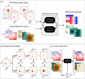


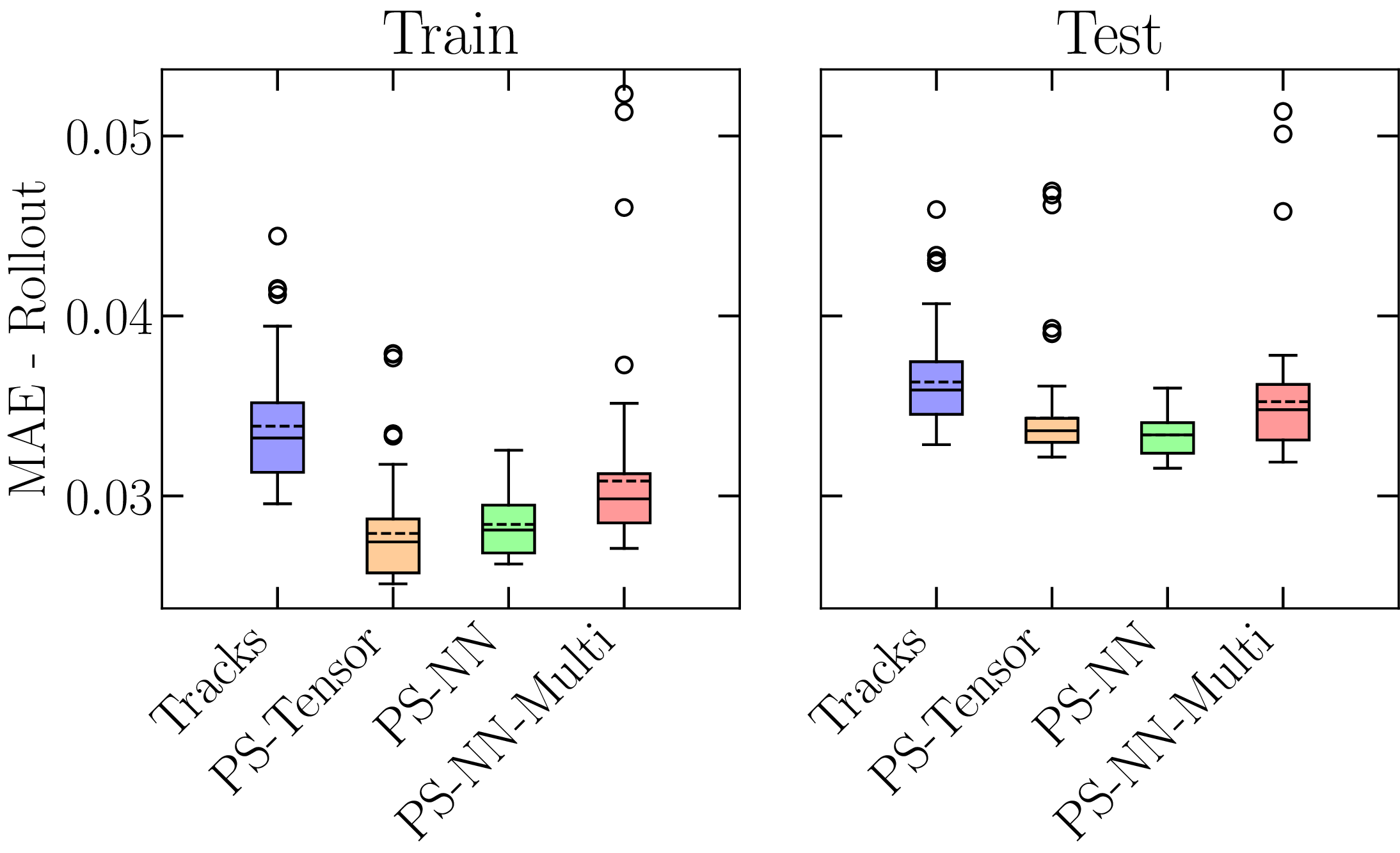


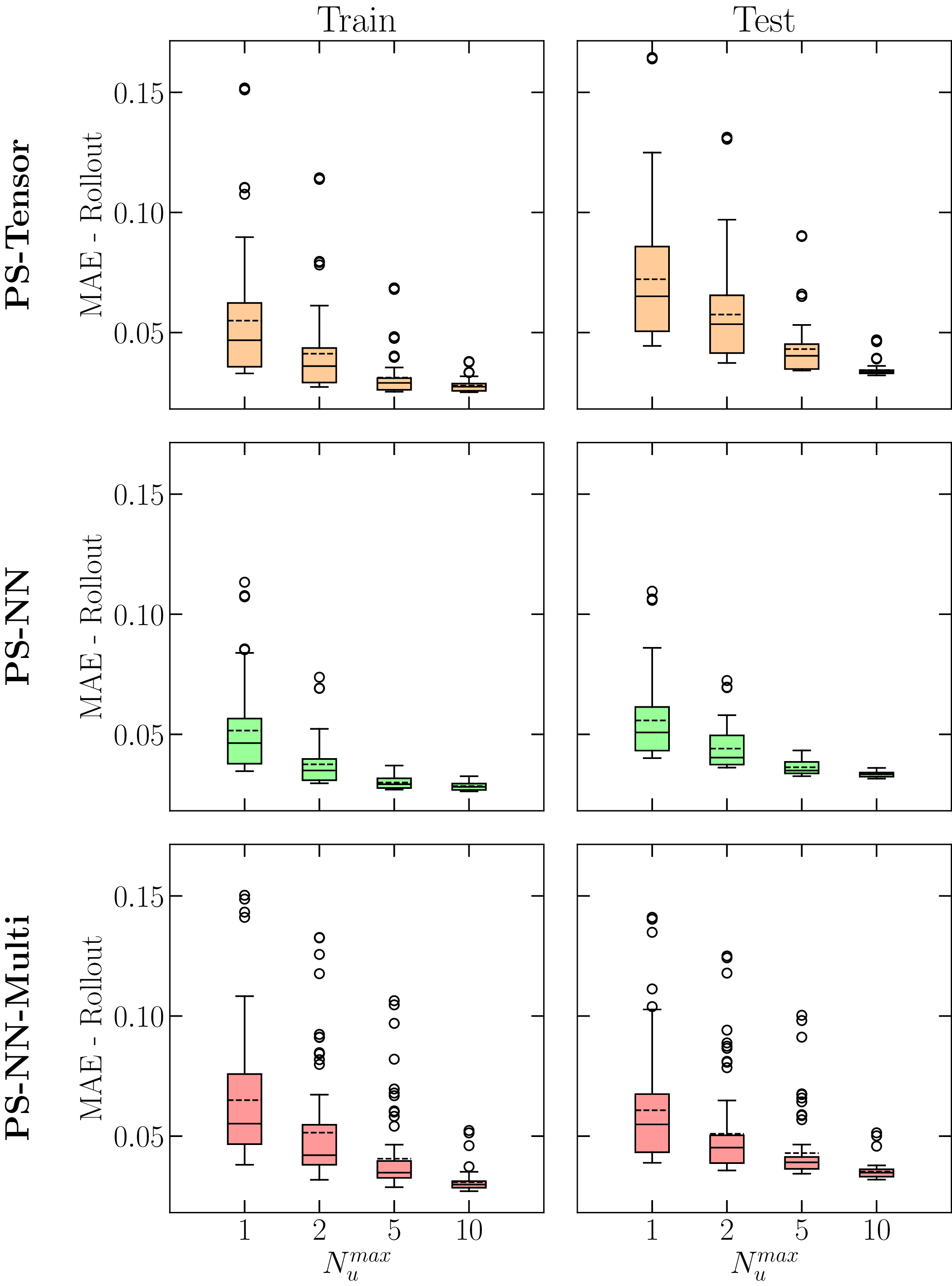


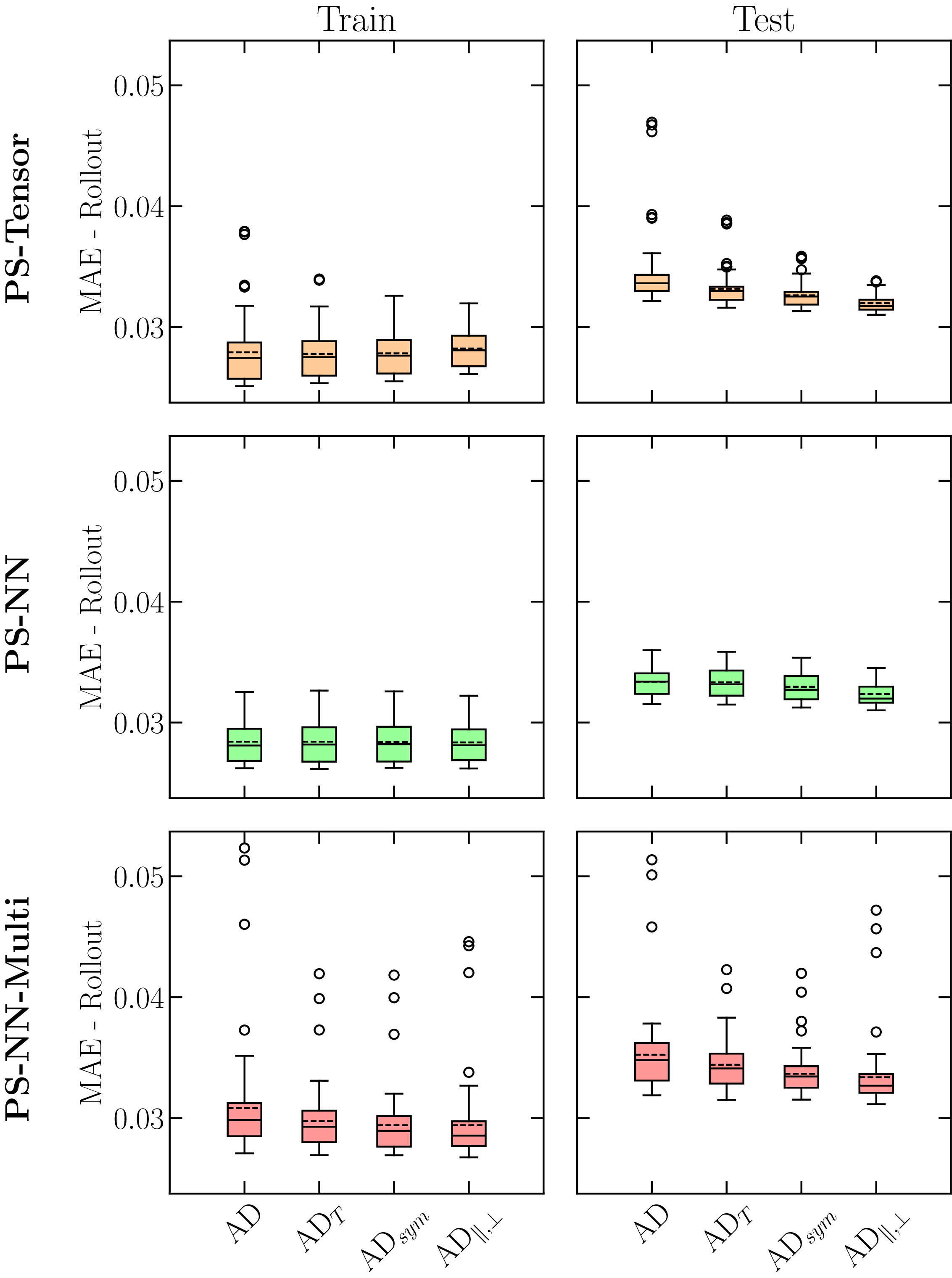


 Open access

