


1 Introduction
In this paper, we are interested in the local dynamics of antiholomorphic diffeomorphisms with a parabolic fixed point, that is, a fixed point of multiplicity
 $k+1$
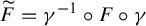
(that is, of codimension k). We study the classification under conjugacy by analytic changes of coordinate of a germ of an antiholomorphic diffeomorphism f with a parabolic fixed point. In a local coordinate, it may be chosen in the form
$k+1$
(that is, of codimension k). We study the classification under conjugacy by analytic changes of coordinate of a germ of an antiholomorphic diffeomorphism f with a parabolic fixed point. In a local coordinate, it may be chosen in the form
 $$ \begin{align} \textstyle f(z) = {\overline z} + {1\over2} {\overline z}^{k+1} + o({\overline z}^{k+1}) \end{align} $$
for some integer
 $k \geq 1$
.
$k \geq 1$
.
The classification of parabolic fixed points in the holomorphic case for a germ
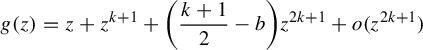 $$ \begin{align} g(z) = z + z^{k+1} + \bigg({k+1\over 2}-b\bigg)z^{2k+1} + o(z^{2k+1}) \end{align} $$
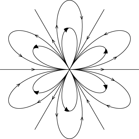
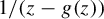
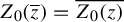
is well known. (See e.g. [Reference Ilyashenko5] or [Reference Ilyashenko and Yakovenko6].) The dynamics of g (see Figure 1) is determined by a topological invariant, the integer k, a formal invariant, the complex number b, and an analytic invariant given by an equivalence class of
 $2k$
germs of diffeomorphisms which are the transition functions on the space of orbits of g (the Écalle horn maps). Two germs
$2k$
germs of diffeomorphisms which are the transition functions on the space of orbits of g (the Écalle horn maps). Two germs
 $g_1$
and
$g_1$
and
 $g_2$
are formally equivalent if and only if they have the same topological invariant and formal invariant. Furthermore, they are analytically equivalent if and only if they also have the same analytic invariant.
$g_2$
are formally equivalent if and only if they have the same topological invariant and formal invariant. Furthermore, they are analytically equivalent if and only if they also have the same analytic invariant.
The goal of this paper is to establish a local classification of antiholomorphic parabolic germs under analytic conjugation and to describe the space of orbits of such a germ and, more generally, to explore the geometric properties of antiholomorphic parabolic germs which are invariant under analytic conjugation. This is done for fixed points of any multiplicity. It allows us to provide a solution to the following problems.
Dynamics of a holomorphic parabolic germ with topological invariant
 $k=3$
.
$k=3$
.
Questions 1.1.
-
(1) (Antiholomorphic root extraction) The second iterate of an antiholomorphic parabolic germ f as in equation (1) is a holomorphic germ which is parabolic. When is the converse true: given a parabolic germ of a holomorphic diffeomorphism g, when is it possible to write it as
 $g = f\circ f$
for some antiholomorphic parabolic germ f? We call f an antiholomorphic square root of g. More generally, when does g have an antiholomorphic root of some order?
$g = f\circ f$
for some antiholomorphic parabolic germ f? We call f an antiholomorphic square root of g. More generally, when does g have an antiholomorphic root of some order? -
(2) Analogously, when does an antiholomorphic parabolic germ have an antiholomorphic root? When are the roots unique?
-
(3) (Embedding) Let
$\{v^t\}_t$
, where
$v^t\colon z\mapsto v^t(z)$
, be the flow of the differential equation
$\dot z = v(z) = (z^{k+1}/(1+bz^k))$
. Each
$v^t$
(
$t{\kern-1pt}\not =0$
) is a holomorphic germ with a parabolic fixed point at the origin. Then
$\overline {v^{\scriptscriptstyle {1/2}}(\cdot )}$
is an antiholomorphic germ and any antiholomorphic parabolic germ is formally conjugate to such a germ. Given an antiholomorphic parabolic germ f, when is it analytically conjugate to some
$\overline {v^{\scriptscriptstyle {1/2}}(\cdot )}$
? In that case, it allows us to embed f in the family
$\overline {v^t}$
. -
(4) When does an antiholomorphic germ preserve a germ of a real analytic curve? This is equivalent to saying that the germ is analytically conjugate to a germ with real coefficients.
-
(5) (Centralizer) Can we describe all the antiholomorphic parabolic germs f that commute with a holomorphic parabolic germ g? If f and g commute, then f sends the orbits of g on the orbits of g. This greatly restricts the possible f. In an analogous way, can we describe all the holomorphic and the antiholomorphic germs that commute with an antiholomorphic parabolic germ?


The above problems are questions about the equivalence classes of germs under analytic conjugacy. Therefore, the answer should be read in the modulus of classification, which will be introduced in §5. At the time of going to press, we learnt of the recent paper [Reference Inou and Mukherjee7], where the authors raised similar types of questions about antiholomorphic polynomial maps with a parabolic germ. It seems plausible that the local theory developed in this paper can help solving some of these questions.
The local dynamics of an antiholomorphic parabolic germ has similarities with the holomorphic case: indeed, the nth iterate
 $f^{\circ n}$
is holomorphic for n even. We find that the dynamics is determined by the same topological and formal invariants, but the analytic invariant is composed of k germs of diffeomorphisms, instead of
$f^{\circ n}$
is holomorphic for n even. We find that the dynamics is determined by the same topological and formal invariants, but the analytic invariant is composed of k germs of diffeomorphisms, instead of
 $2k$
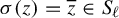
. This is explained by the fact that an orbit of f will usually jump between two Fatou petals of its associated holomorphic parabolic germ
$2k$
. This is explained by the fact that an orbit of f will usually jump between two Fatou petals of its associated holomorphic parabolic germ
 $f^{\circ 2}$
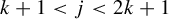
(see Figure 2), so that the dynamics in those petals are not independent.
$f^{\circ 2}$
(see Figure 2), so that the dynamics in those petals are not independent.
An orbit of f jumping between two petals. An orbit of the second iterate
 $f^{\circ 2}$
will remain either in the upper petal or the lower petal.
$f^{\circ 2}$
will remain either in the upper petal or the lower petal.

We observe other differences from the holomorphic case. A holomorphic germ has
 $2k$
formal separatrices. The antiholomorphic germ has instead a privileged unique direction; a formal symmetry axis. There is also a topological difference between the cases where the codimension is odd or even. When k is even, the rotation
$2k$
formal separatrices. The antiholomorphic germ has instead a privileged unique direction; a formal symmetry axis. There is also a topological difference between the cases where the codimension is odd or even. When k is even, the rotation
 $z\mapsto -z$
is a formal symmetry of f, whilst it is not for k odd.
$z\mapsto -z$
is a formal symmetry of f, whilst it is not for k odd.
Antiholomorphic dynamics has been considered before in the context of antipolynomials, that is, a polynomial function of
 ${\overline z}$
,
${\overline z}$
,
 $p(z) = {\overline z}^n + \cdots + a_0$
. Iteration of antipolynomials was studied by Nakane and Schleicher in [Reference Nakane and Schleicher10], Hubbard and Schleicher in [Reference Hubbard and Schleicher4], and Mukherjee, Nakane and Schleicher in [Reference Mukherjee, Nakane and Schleicher9]. Their focus is mostly on the family of antipolynomials
$p(z) = {\overline z}^n + \cdots + a_0$
. Iteration of antipolynomials was studied by Nakane and Schleicher in [Reference Nakane and Schleicher10], Hubbard and Schleicher in [Reference Hubbard and Schleicher4], and Mukherjee, Nakane and Schleicher in [Reference Mukherjee, Nakane and Schleicher9]. Their focus is mostly on the family of antipolynomials
 $p_c(z) = {\overline z}^d + c$
and the description of the connectedness locus
$p_c(z) = {\overline z}^d + c$
and the description of the connectedness locus
 $\mathcal M_d^\ast $
called the multicorn. The context is global in nature, but the local analysis contributes significantly.
$\mathcal M_d^\ast $
called the multicorn. The context is global in nature, but the local analysis contributes significantly.
An important role is played by periodic orbits of
 $p_c$
of odd period k, because when k is odd,
$p_c$
of odd period k, because when k is odd,
 $p_c^{\circ k}$
is antiholomorphic. In this case, all indifferent periodic orbits are parabolic and they occur along real analytic arcs in the parameter space, as proved in [Reference Hubbard and Schleicher4, Reference Mukherjee, Nakane and Schleicher9]. However, only points of codimensions one and two are observed. This is due to a choice of a special subfamily of antipolynomials of degree d. Indeed, higher codimension is already observed in the two-parameter family
$p_c^{\circ k}$
is antiholomorphic. In this case, all indifferent periodic orbits are parabolic and they occur along real analytic arcs in the parameter space, as proved in [Reference Hubbard and Schleicher4, Reference Mukherjee, Nakane and Schleicher9]. However, only points of codimensions one and two are observed. This is due to a choice of a special subfamily of antipolynomials of degree d. Indeed, higher codimension is already observed in the two-parameter family
 ${\overline z}^d + c_1{\overline z} + c_0$
, e.g. when
${\overline z}^d + c_1{\overline z} + c_0$
, e.g. when
 $c_1 = 1$
and
$c_1 = 1$
and
 $c_0=0$
.
$c_0=0$
.
One of the tools used for antipolynomials is called the Écalle height, introduced by Hubbard and Schleicher in [Reference Hubbard and Schleicher4]. In codimension one, on the Écalle cylinder of the attractive petal, the imaginary part of an orbit is intrinsic, and the Écalle height of the critical values is finite. This is used to prove that at the ends of parabolic arcs in the parameter space,
 $p_c$
has a parabolic periodic orbit of odd period of codimension two; see [Reference Hubbard and Schleicher4, §3]. When studying the space of orbits of an antiholomorphic germ of a parabolic diffeomorphism of any codimension, we see that the Écalle height has a meaning only on the Écalle cylinder of the petals containing the formal symmetry axis of f. This is seen by describing the space of orbits on a neighbourhood of a parabolic fixed point, which we do in §6.2.
$p_c$
has a parabolic periodic orbit of odd period of codimension two; see [Reference Hubbard and Schleicher4, §3]. When studying the space of orbits of an antiholomorphic germ of a parabolic diffeomorphism of any codimension, we see that the Écalle height has a meaning only on the Écalle cylinder of the petals containing the formal symmetry axis of f. This is seen by describing the space of orbits on a neighbourhood of a parabolic fixed point, which we do in §6.2.
The paper is organized as follows. In §2, we define the topological and formal invariants of f. We also establish a formal normal form for f.
In §3, we study the formal normal form.
In §4, we introduce the rectifying coordinate and the Fatou coordinates in order to define the transition functions (Definition 5.4) in §5, which is the analytic invariant. This leads to the modulus of classification of f.
In §6.1, we recall a description of the space of orbits in the holomorphic case using
 $2k$
spheres (or Écalle cylinders) glued with the horn maps (these are the expressions of the transition functions in the coordinates of the spheres). We use this space of orbits in §6.2 to identify the space of orbits of f to a manifold of real dimension two by quotienting the space of orbits of
$2k$
spheres (or Écalle cylinders) glued with the horn maps (these are the expressions of the transition functions in the coordinates of the spheres). We use this space of orbits in §6.2 to identify the space of orbits of f to a manifold of real dimension two by quotienting the space of orbits of
 $f\circ f$
by the action of f.
$f\circ f$
by the action of f.
After describing the space of orbits, we state, in §6.3, the main result of the paper: the classification theorem (Theorem 6.3). The idea in spirit is that two germs are equivalent if and only if their spaces of orbits are equivalent; the classification theorem is a way to rigorously express this statement.
Finally, with the classification theorem in hand, in §7 we answer Questions (1) to (5) of this introduction.
2 Antiholomorphic parabolic fixed points
Notation 2.1. For the whole paper, we will use the following notation:
-
•
$\sigma (z) = {\overline z}$
is the complex conjugation; -
•
$\tau (w) = {1/\overline w}$
is the antiholomorphic inversion; -
•
$T_C(Z) = Z + C$
is the translation by
$C\in \mathbb {C}$
; -
•
$L_c(w) = cw$
is the linear transformation with multiplier
$c\in \mathbb {C}$
; -
•
$v^t$
is the time-t of the vector field (3)
$$ \begin{align}{\dot z} = v(z) = \frac{z^{k+1}}{1 + bz^k}.\end{align} $$


A function
 $f\colon U \to \mathbb {C}$
defined on a domain
$f\colon U \to \mathbb {C}$
defined on a domain
 $U\subseteq \mathbb {C}$
is antiholomorphic if
$U\subseteq \mathbb {C}$
is antiholomorphic if
 ${\partial f/ \partial z} \equiv 0$
on U. From this definition, together with the chain rule, it follows that antiholomorphy is an intrinsic property of f under holomorphic changes of variable. Equivalently,
${\partial f/ \partial z} \equiv 0$
on U. From this definition, together with the chain rule, it follows that antiholomorphy is an intrinsic property of f under holomorphic changes of variable. Equivalently,
 $f\colon z\mapsto f(z)$
is antiholomorphic if
$f\colon z\mapsto f(z)$
is antiholomorphic if
 $f\circ \sigma \colon z\mapsto f({\overline z})$
is holomorphic; therefore,
$f\circ \sigma \colon z\mapsto f({\overline z})$
is holomorphic; therefore,
 $f(z)$
expands in a power series in terms of
$f(z)$
expands in a power series in terms of
 ${\overline z}$
.
${\overline z}$
.
Note that the multiplier at a fixed point of an antiholomorphic function is not intrinsic; only its modulus is. Indeed, a scaling of
 $\unicode{x3bb} $
will add a factor of
$\unicode{x3bb} $
will add a factor of
 $\unicode{x3bb} /\overline {\unicode{x3bb} }$
to the multiplier.
$\unicode{x3bb} /\overline {\unicode{x3bb} }$
to the multiplier.
Definition 2.2. (Parabolic fixed point)
A germ of an antiholomorphic diffeomorphism fixing the origin
 $f\colon (\mathbb {C},0)\to (\mathbb {C},0)$
has a parabolic fixed point at
$f\colon (\mathbb {C},0)\to (\mathbb {C},0)$
has a parabolic fixed point at
 $0$
if
$0$
if
 $0$
is an isolated fixed point and
$0$
is an isolated fixed point and
 $$ \begin{align*}\bigg|{\partial f\over \partial {\overline z}}(0)\bigg| = 1. \end{align*} $$
We will also say that f is an antiholomorphic parabolic germ.
Proposition 2.3. Let
 $f(z) = a_1{\overline z} + a_2 {\overline z}^2 + a_3 {\overline z}^3 + \cdots $
. If
$f(z) = a_1{\overline z} + a_2 {\overline z}^2 + a_3 {\overline z}^3 + \cdots $
. If
 $|a_1| = 1$
, then f is formally conjugate to a formal power series
$|a_1| = 1$
, then f is formally conjugate to a formal power series
 $$ \begin{align} {f^{\dagger}}(w) = {\overline w} + \sum_{n=2}^\infty A_n {\overline w}^n \end{align} $$
with real coefficients
 $A_n$
. If there exists
$A_n$
. If there exists
 $n \geq 2$
such that
$n \geq 2$
such that
 $A_n{\kern-1pt}\not =0$
, then
$A_n{\kern-1pt}\not =0$
, then
 $0$
is a parabolic fixed point of f. Let
$0$
is a parabolic fixed point of f. Let
 $n_0 =k+1$
be the minimum such n. Then a scaling brings
$n_0 =k+1$
be the minimum such n. Then a scaling brings
 $A_{k+1}$
to
$A_{k+1}$
to
 $\tfrac 12$
if k is odd (respectively
$\tfrac 12$
if k is odd (respectively
 $\pm \tfrac 12$
if k is even).
$\pm \tfrac 12$
if k is even).
Proof The proof is a mere computation. Let
 $w = {\widehat h}(z) = \sum _{n\geq 1} b_n z^n$
be a formal change of coordinate and suppose that
$w = {\widehat h}(z) = \sum _{n\geq 1} b_n z^n$
be a formal change of coordinate and suppose that
 ${f^{\dagger }}(w) = {\overline w} + \sum _{n\geq 2} A_n {\overline w}^n$
. If we compare
${f^{\dagger }}(w) = {\overline w} + \sum _{n\geq 2} A_n {\overline w}^n$
. If we compare
 $h\circ f(z) = {f^{\dagger }} \circ h(z)$
degree by degree, we find an expression for the coefficients of the form
$h\circ f(z) = {f^{\dagger }} \circ h(z)$
degree by degree, we find an expression for the coefficients of the form
 $$ \begin{align*}\begin{cases} b_1a_1 = \overline{b_1},\\[2pt] A_n = b_n - \overline{b_n} + a_n + P_n(A_1,\ldots, A_{n-1}, a_1,\ldots,a_{n-1}, b_1,\ldots, b_{n-1}), \end{cases} \end{align*} $$
where
 $P_n$
is some polynomial. Hence, we have
$P_n$
is some polynomial. Hence, we have
 $\arg b_1 = -{\tfrac 12} \arg a_1 + \ell \pi $
with
$\arg b_1 = -{\tfrac 12} \arg a_1 + \ell \pi $
with
 $\ell \in \mathbb {Z}$
. With a recursive argument, if
$\ell \in \mathbb {Z}$
. With a recursive argument, if
 $A_1,\ldots , A_{n-1}$
are real, for
$A_1,\ldots , A_{n-1}$
are real, for
 $A_n$
to be real, we may choose
$A_n$
to be real, we may choose
 $\textrm{Im}\kern2pt b_n = {\tfrac 12}\textrm{Im}\kern2pt (a_n + P_n)$
, since
$\textrm{Im}\kern2pt b_n = {\tfrac 12}\textrm{Im}\kern2pt (a_n + P_n)$
, since
 $P_n$
depends only on terms that were fixed in the previous steps.
$P_n$
depends only on terms that were fixed in the previous steps.
Remark 2.4. The formal change of coordinate
 ${\widehat h}$
is not unique. Indeed, only the imaginary parts of the coefficients are determined, leaving their real parts free. However, the order of the first nonlinear term is well defined. This leads to the following definition.
${\widehat h}$
is not unique. Indeed, only the imaginary parts of the coefficients are determined, leaving their real parts free. However, the order of the first nonlinear term is well defined. This leads to the following definition.
Definition 2.5. We say that f is parabolic of codimension k if the first nonlinear term of
 ${f^{\dagger }}$
is of order
${f^{\dagger }}$
is of order
 $k+1$
.
$k+1$
.
Remarks 2.6.
-
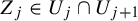
(1) The formal series with real coefficients preserves the real axis. This indicates that f has a privileged unique direction, which we will call a formal symmetry axis. Hence, a conjugacy between two antiholomorphic parabolic germs must preserve the formal symmetry axis. We can of course suppose that this formal axis is the real axis. Note however that in the case of even codimension, there is no canonical orientation of the formal symmetry axis.
-
(2) The dynamics near the formal symmetry axis is a topological invariant. When k is odd, a rotation of angle
$\pi $
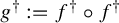
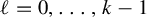
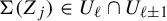
will flip the attractive semi-axis with the repulsive one. When k is even, both semi-axes are either attractive (when
$A_{k+1} < 0$
) or repulsive (when
$A_{k+1}> 0$
) (see Figures 3 and 4). In this paper, we will only consider the case
$A_{k+1}> 0$
. Indeed, when
$A_{k+1} < 0 $
, that is, f is of negative type, then
$f^{-1}$
will be of positive type and classifying
$f^{-1}$
is equivalent to classifying f.


Definition 2.7. When the codimension k is even, we say that f is of positive type (respectively negative type) if
 $A_{k+1}> 0$
(respectively
$A_{k+1}> 0$
(respectively
 $A_{k+1} < 0$
), where
$A_{k+1} < 0$
), where
 $A_{k+1}$
is the first non-zero coefficient in (4).
$A_{k+1}$
is the first non-zero coefficient in (4).
The composition of two antiholomorphic germs is holomorphic. Therefore, we will look at
 $g:= f\circ f$
, which is a holomorphic parabolic germ. Recall that in the holomorphic case, the codimension of g is the order of the first non-zero term of
$g:= f\circ f$
, which is a holomorphic parabolic germ. Recall that in the holomorphic case, the codimension of g is the order of the first non-zero term of
 $g(z) - z$
. It is linked to the multiplicity of the fixed point: g is of codimension k if and only if the fixed point has multiplicity
$g(z) - z$
. It is linked to the multiplicity of the fixed point: g is of codimension k if and only if the fixed point has multiplicity
 $k+1$
.
$k+1$
.
Corollary 2.8.
f is of codimension k if only if
 $g = f\circ f$
is of codimension k.
$g = f\circ f$
is of codimension k.
The case when
 $f \circ f = \mathrm {id}$
is seen as a degenerate case where f is of ‘codimension infinity’. Indeed, it only happens if f is analytically conjugate to the complex conjugation, as is shown below. This case was excluded from our definition of parabolic point, since the fixed point of
$f \circ f = \mathrm {id}$
is seen as a degenerate case where f is of ‘codimension infinity’. Indeed, it only happens if f is analytically conjugate to the complex conjugation, as is shown below. This case was excluded from our definition of parabolic point, since the fixed point of
 $\sigma $
at the origin is not isolated.
$\sigma $
at the origin is not isolated.
Proposition 2.9. Let
 $f(z) = a_1{\overline z} + a_2 {\overline z}^2 + a_3 {\overline z}^3 + \cdots $
be an antiholomorphic germ at the origin. The following statements are equivalent:
$f(z) = a_1{\overline z} + a_2 {\overline z}^2 + a_3 {\overline z}^3 + \cdots $
be an antiholomorphic germ at the origin. The following statements are equivalent:
-
(1) f is formally conjugate to
$\sigma $
; -
(2) f is analytically conjugate to
$\sigma $
; -
(3)
$f\circ f = \mathrm {id}$
.


Dynamics near the formal symmetry axis of
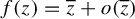 $f(z) = {\overline z} + o({\overline z})$
in odd codimension. One sector is attractive and the other repulsive; this yields the two possibilities above.
$f(z) = {\overline z} + o({\overline z})$
in odd codimension. One sector is attractive and the other repulsive; this yields the two possibilities above.
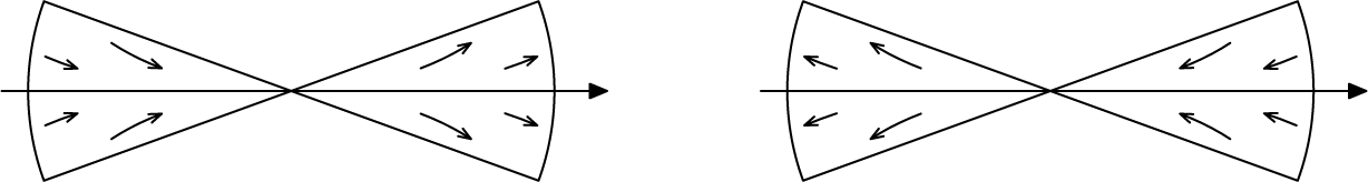
Dynamics near the formal symmetry axis of
 $f(z) = {\overline z} + o({\overline z})$
in even codimension. The possibilities are: on the left, both sectors are repulsive (positive type) and, on the right, both are attractive (negative type).
$f(z) = {\overline z} + o({\overline z})$
in even codimension. The possibilities are: on the left, both sectors are repulsive (positive type) and, on the right, both are attractive (negative type).

Proof
 $(1)\Rightarrow (3)$
Since there is a formal change of coordinate m such that
$(1)\Rightarrow (3)$
Since there is a formal change of coordinate m such that
 $m\circ f\circ m^{-1} = \sigma $
, we have
$m\circ f\circ m^{-1} = \sigma $
, we have
 $m \circ f\circ f\circ m^{-1} = \mathrm {id}$
formally, which yields
$m \circ f\circ f\circ m^{-1} = \mathrm {id}$
formally, which yields
 $f\circ f = \mathrm {id}$
.
$f\circ f = \mathrm {id}$
.
 $(3)\Rightarrow (2)$
Let us suppose that
$(3)\Rightarrow (2)$
Let us suppose that
 $f\circ f=\mathrm {id}$
. In particular,
$f\circ f=\mathrm {id}$
. In particular,
 $|a_1| = 1$
. We can of course suppose that f is already in a coordinate such that
$|a_1| = 1$
. We can of course suppose that f is already in a coordinate such that
 $a_1 = 1$
.
$a_1 = 1$
.
Let
 $F_1(x,y) = \Re f(z)$
and
$F_1(x,y) = \Re f(z)$
and
 $F_2(x,y) = \textrm{Im}\kern2pt f(z)$
; then we have
$F_2(x,y) = \textrm{Im}\kern2pt f(z)$
; then we have
 $$ \begin{align*}F(x,y) = \begin{pmatrix} F_1(x,y)\cr F_2(x,y) \end{pmatrix} = \begin{pmatrix} x + O(|(x,y)|^2)\cr -y + O(|(x,y)|^2)\cr\end{pmatrix}. \end{align*} $$
We are interested in the fixed points of F, that is, the zeros of
 $F-\mathrm {id}$
. Since
$F-\mathrm {id}$
. Since
 $(\partial / \partial y)(F_2(x,y) - y)|_{(0,0)} = -2$
, by the implicit function theorem, there exists an analytic curve
$(\partial / \partial y)(F_2(x,y) - y)|_{(0,0)} = -2$
, by the implicit function theorem, there exists an analytic curve
 $\gamma \colon t\mapsto t + i\eta (t)$
such that
$\gamma \colon t\mapsto t + i\eta (t)$
such that
 $F_2(x,y) - y = 0$
if and only if
$F_2(x,y) - y = 0$
if and only if
 $y = \eta (x)$
.
$y = \eta (x)$
.
We complexify t to obtain a change of coordinate
 $t = \gamma ^{-1}(z) = u + iv$
that rectifies the curve
$t = \gamma ^{-1}(z) = u + iv$
that rectifies the curve
 $\gamma $
on the real line. Let
$\gamma $
on the real line. Let
 $\tilde {f} = \gamma ^{-1}\circ f\circ \gamma $
. In the new coordinate,
$\tilde {f} = \gamma ^{-1}\circ f\circ \gamma $
. In the new coordinate,
 $\widetilde F = \gamma ^{-1}\circ F\circ \gamma $
has now the form
$\widetilde F = \gamma ^{-1}\circ F\circ \gamma $
has now the form
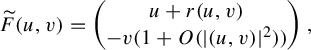 $$ \begin{align*}\widetilde F(u,v) = \begin{pmatrix} u + r(u,v) \cr -v(1 + O(|(u,v)|^2)) \end{pmatrix}, \end{align*} $$
where
 $r(u,v) = O(|(u,v)|^2)$
. The equation for fixed points
$r(u,v) = O(|(u,v)|^2)$
. The equation for fixed points
 $\widetilde F = \mathrm {id}$
is equivalent to
$\widetilde F = \mathrm {id}$
is equivalent to
 $v=0$
and
$v=0$
and
 $r(u,0) = 0$
. If
$r(u,0) = 0$
. If
 $r(u,0) = au^s + o(u^s)$
,
$r(u,0) = au^s + o(u^s)$
,
 $a{\kern-1pt}\not =0$
, then this would contradict the fact that we must have
$a{\kern-1pt}\not =0$
, then this would contradict the fact that we must have
 $\widetilde F\circ \widetilde F(u,0) = ({u\atop 0})$
. Therefore,
$\widetilde F\circ \widetilde F(u,0) = ({u\atop 0})$
. Therefore,
 $r(u,0) \equiv 0$
; in other words,
$r(u,0) \equiv 0$
; in other words,
 $r(u,v) = v p(u,v)$
.
$r(u,v) = v p(u,v)$
.
We see that the real axis is a line of fixed points for
 $\tilde {f}$
near the origin. By the identity theorem, because
$\tilde {f}$
near the origin. By the identity theorem, because
 $\tilde {f}\circ \sigma - \mathrm {id} = 0$
on the real axis near the origin, we have
$\tilde {f}\circ \sigma - \mathrm {id} = 0$
on the real axis near the origin, we have
 $\tilde {f} \equiv \sigma $
.
$\tilde {f} \equiv \sigma $
.
 $(2)\Rightarrow (1)$
This is immediate.
$(2)\Rightarrow (1)$
This is immediate.
The formal power series with real coefficients is used to determine a formal normal form for f. Recall that a formal normal form for
 $g:=f \circ f$
may be taken as the time-one map of the flow of (see [Reference Ilyashenko and Yakovenko6])
$g:=f \circ f$
may be taken as the time-one map of the flow of (see [Reference Ilyashenko and Yakovenko6])
 $$ \begin{align} {\dot z} = {z^{k+1} \over 1 + bz^k} \end{align} $$
for some constant
 $b\in \mathbb {C}$
. We will call this constant b the formal invariant. It is also sometimes called the ‘résidu itératif’ and, as mentioned in [Reference Hubbard and Schleicher4], it is determined by the holomorphic fixed point index, that is, the residue of
$b\in \mathbb {C}$
. We will call this constant b the formal invariant. It is also sometimes called the ‘résidu itératif’ and, as mentioned in [Reference Hubbard and Schleicher4], it is determined by the holomorphic fixed point index, that is, the residue of
 ${1 /( z - g(z))}$
at the origin.
${1 /( z - g(z))}$
at the origin.
When
 $g = f\circ f$
is of codimension k, it is possible to get rid of the terms of degree
$g = f\circ f$
is of codimension k, it is possible to get rid of the terms of degree
 $k+1 < j < 2k+1$
by an analytic change of coordinate. In this coordinate, g is written as
$k+1 < j < 2k+1$
by an analytic change of coordinate. In this coordinate, g is written as
 $$ \begin{align} g(z) = z + z^{k+1} + \bigg( {k+1 \over 2} - b\bigg)z^{2k +1} + o(z^{2k + 1}), \end{align} $$
where
 $b\in \mathbb {C}$
is the formal invariant of g. When g is in this form, we will say that it is prenormalized.
$b\in \mathbb {C}$
is the formal invariant of g. When g is in this form, we will say that it is prenormalized.
Definition 2.10. The formal invariant of f is the formal invariant of
 $f \circ f$
, which is the constant b in (6).
$f \circ f$
, which is the constant b in (6).
As the name suggests, b is invariant under formal changes of coordinate. Since
 ${g^{\dagger }} := {f^{\dagger }} \circ {f^{\dagger }}$
and g have the same formal invariant, where
${g^{\dagger }} := {f^{\dagger }} \circ {f^{\dagger }}$
and g have the same formal invariant, where
 ${f^{\dagger }}$
is as in (4), it follows that b is real because all the coefficients of
${f^{\dagger }}$
is as in (4), it follows that b is real because all the coefficients of
 ${g^{\dagger }}$
are real.
${g^{\dagger }}$
are real.
An important consequence of this is that the time-t map
 $v^t$
of (5) for
$v^t$
of (5) for
 $t\in \mathbb {R}$
has a power series at
$t\in \mathbb {R}$
has a power series at
 $0$
with real coefficients, that is, the complex conjugation
$0$
with real coefficients, that is, the complex conjugation
 $\sigma $
and
$\sigma $
and
 $v^t$
commute.
$v^t$
commute.
Proposition 2.11. Let
 $v^{\scriptscriptstyle {1/2}}$
be the time-
$v^{\scriptscriptstyle {1/2}}$
be the time-
 ${\tfrac 12}$
of the vector field (5) for some b. If f is of codimension k, of positive type if k is even, and if f has formal invariant b, then f and
${\tfrac 12}$
of the vector field (5) for some b. If f is of codimension k, of positive type if k is even, and if f has formal invariant b, then f and
 $\sigma \circ v^{\scriptscriptstyle {1/2}}$
are formally conjugate.
$\sigma \circ v^{\scriptscriptstyle {1/2}}$
are formally conjugate.
Proof Let
 ${f^{\dagger }}$
be the formal power series with real coefficients formally conjugate to f in Proposition 2.3. Then
${f^{\dagger }}$
be the formal power series with real coefficients formally conjugate to f in Proposition 2.3. Then
 ${f^{\dagger }}\circ \sigma $
is a parabolic formal power series of z. A formal normal form may be chosen as
${f^{\dagger }}\circ \sigma $
is a parabolic formal power series of z. A formal normal form may be chosen as
 $v^{\scriptscriptstyle {1/2}}$
, the time-
$v^{\scriptscriptstyle {1/2}}$
, the time-
 $\tfrac 12$
of the vector field (5). Since both the coefficients of
$\tfrac 12$
of the vector field (5). Since both the coefficients of
 $v^{\scriptscriptstyle {1/2}}$
and
$v^{\scriptscriptstyle {1/2}}$
and
 ${f^{\dagger }}$
are real, the formal change of coordinate h commutes with
${f^{\dagger }}$
are real, the formal change of coordinate h commutes with
 $\sigma $
, provided that
$\sigma $
, provided that
 $h'(0) = 1$
, so that
$h'(0) = 1$
, so that
 $v^{\scriptscriptstyle {1/2}}\circ \sigma $
is formally conjugate to f.
$v^{\scriptscriptstyle {1/2}}\circ \sigma $
is formally conjugate to f.
The formal change of coordinate conjugating f to its formal normal form can always be truncated at the
 $(2k+2)$
th term, which yields a holomorphic change of coordinate taking f to the form
$(2k+2)$
th term, which yields a holomorphic change of coordinate taking f to the form
 $$ \begin{align} f(z) = {\overline z} + {1\over 2}{\overline z}^{k+1} + \bigg({k+1 \over 8} - {b \over 2}\bigg){\overline z}^{2k+1} + o({\overline z}^{2k+1}), \end{align} $$
that is, f and
 $\sigma \circ v^{\scriptscriptstyle {1/2}}$
have the same first three terms.
$\sigma \circ v^{\scriptscriptstyle {1/2}}$
have the same first three terms.
Definition 2.12. When f is in the form (7), we will say that it is prenormalized.
Remark 2.13. In even codimension, f may only be prenormalized as in (7) when
 $A_{k+1}> 0$
. In odd codimension, f may always be prenormalized as in (7).
$A_{k+1}> 0$
. In odd codimension, f may always be prenormalized as in (7).
The formal normal form is a model to which the germs can be compared. Now that this form has been established, we describe its properties.
3 Properties of the formal normal form
Let us start with the following observations.
Proposition 3.1. Let v be the vector field (5) of codimension k and formal invariant b.
-
(1) v is invariant under the rotations of order k.
-
(2) v is invariant under the complex conjugation
$\sigma $
when b is real.

The holomorphic and antiholomorphic formal normal forms are respectively
 $$ \begin{align} v^1(z) &= z + z^{k+1} + \bigg({k+1\over 2} - b\bigg)z^{2k+1} + o(z^{2k+1}), \end{align} $$
 $$ \begin{align} \sigma\circ v^{\scriptscriptstyle{1/2}}(z) &= {\overline z} + {1\over2}{\overline z}^{k+1} + \bigg({k+1\over 8} - {b\over 2}\bigg){\overline z}^{2k+1} + o({\overline z}^{2k+1}), \end{align} $$
where
 $v^t$
is the time-t of v.
$v^t$
is the time-t of v.
We see that the real axis is a symmetry axis. We introduce a notation for the other symmetry axes.
Definition 3.2. Let
 $\sigma _\ell $
denote the reflection
$\sigma _\ell $
denote the reflection
 $$ \begin{align} \sigma_\ell(z) := e^{2i\pi\ell/ k} {\overline z} \qquad\textrm{for }\ell=0,\ldots,k-1. \end{align} $$
Corollary 3.3.
-
(1) v is invariant under
$\sigma _\ell $
for
$\ell =0,\ldots ,k-1$
when b is real. -
(2)
$v^{\scriptscriptstyle 1}$
commutes with any rotation of order k and, when b is real, it commutes with
$\sigma _\ell $
for
$\ell = 0,\ldots ,k-1$
. -
(3) When k is even,
$\sigma \circ v^{\scriptscriptstyle {1/2}}$
commutes with
$z\mapsto -z$
.


We will only be interested in real values of b.
Proposition 3.4. (Roots of the normal forms)
-
(1) For n even,
$v^{\scriptscriptstyle 1}$
has k one-parameter families of antiholomorphic nth roots given by
$\sigma _\ell \circ v^{\scriptscriptstyle (1/n) + iy}$
for
$y\in \mathbb {R}$
,
$\ell =0,\ldots ,k-1$
. -
(2) For n odd,
$\sigma \circ v^{\scriptscriptstyle {1/2}}$
has exactly one antiholomorphic nth root given by
$\sigma \circ v^{\scriptscriptstyle 1/2n}$
.


We ask the following questions, which will be answered in §7.2.
Question 3.5. For a holomorphic parabolic germ g, how many distinct antiholomorphic nth roots (n even) does it have?
Question 3.6. For an antiholomorphic parabolic germ f and n odd, when is the formal nth root convergent?
4 Fatou coordinates
For the whole section, when the codimension of f is even, we will suppose that f is of positive type (see Definition 2.6). The formal normal form
 $\sigma \circ v^{\scriptscriptstyle {1/2}}$
is a model to which it is natural to compare the antiholomorphic germ f. In the holomorphic study of parabolic germs, we use holomorphic diffeomorphisms called Fatou coordinates defined on sectors covering the origin on which the germ is conjugated to its normal form, that is, changes of coordinates to the normal form. We then compare Fatou coordinates on the intersection of the sectors, thus yielding a conformal invariant describing the space of orbits of the germ. See [Reference Ilyashenko5] or [Reference Ilyashenko and Yakovenko6] for the details.
$\sigma \circ v^{\scriptscriptstyle {1/2}}$
is a model to which it is natural to compare the antiholomorphic germ f. In the holomorphic study of parabolic germs, we use holomorphic diffeomorphisms called Fatou coordinates defined on sectors covering the origin on which the germ is conjugated to its normal form, that is, changes of coordinates to the normal form. We then compare Fatou coordinates on the intersection of the sectors, thus yielding a conformal invariant describing the space of orbits of the germ. See [Reference Ilyashenko5] or [Reference Ilyashenko and Yakovenko6] for the details.
The same approach can be adapted to the antiholomorphic case. It will be necessary to find a sectorial normalization (Fatou coordinates) of the antiholomorphic germ f. However, instead of adapting the construction of the holomorphic case, we will prove that it is possible to choose Fatou coordinates of
 $f \circ f$
, which is holomorphic, that are also Fatou coordinates of f.
$f \circ f$
, which is holomorphic, that are also Fatou coordinates of f.
4.1 Rectifying coordinates and sectors
Suppose that an antiholomorphic parabolic germ f is of codimension k for
 $k\geq 1$
with a formal invariant b (see Definition 2.9). The Fatou coordinates
$k\geq 1$
with a formal invariant b (see Definition 2.9). The Fatou coordinates
 $\varphi _j$
are often constructed in the rectifying coordinate given by the time of the vector field (5). Since
$\varphi _j$
are often constructed in the rectifying coordinate given by the time of the vector field (5). Since
 $v^{\scriptscriptstyle {1/2}}$
and
$v^{\scriptscriptstyle {1/2}}$
and
 $v^{\scriptscriptstyle 1}$
are the time maps of the vector field (5), we define the time coordinate by
$v^{\scriptscriptstyle 1}$
are the time maps of the vector field (5), we define the time coordinate by
 $$ \begin{align} Z(z) = \int_{z_0}^z {1 + b\zeta^k \over \zeta^{k+1}}\mathrm{d}\zeta = -{ 1\over kz^k} + b\log z + {1 \over kz_0^k} - b\log z_0, \end{align} $$
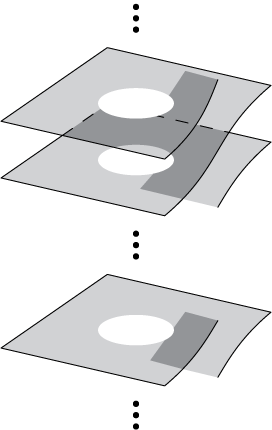
which is multi-valued. See Figure 5 for its Riemann surface. It is the inverse of the flow of (5) with starting point
 $z_0$
. We will single out the following
$z_0$
. We will single out the following
 $2k+1$
charts of Z:
$2k+1$
charts of Z:
 $$ \begin{align} Z_j(z) &= -{1 \over kz^k} + b\log z - {ji\pi b\over k}\nonumber\\ &\quad \textrm{for}\ j=-k,\ldots,-1,0,1,\ldots,k, \end{align} $$
where
 $\log z$
is determined by
$\log z$
is determined by
 $\arg z\in (-\pi ,\pi )$
for
$\arg z\in (-\pi ,\pi )$
for
 $-k < j < k$
and, for
$-k < j < k$
and, for
 $Z_k$
(respectively
$Z_k$
(respectively
 $Z_{-k}$
),
$Z_{-k}$
),
 $\arg (\cdot )$
will be the continuation in
$\arg (\cdot )$
will be the continuation in
 $(0,2\pi )$
(respectively in
$(0,2\pi )$
(respectively in
 $(-2\pi ,0)$
). In particular, we see that
$(-2\pi ,0)$
). In particular, we see that
 $Z_k = Z_{-k}$
, and that both
$Z_k = Z_{-k}$
, and that both
 $Z_0$
and
$Z_0$
and
 $Z_k$
commute with the complex conjugation.
$Z_k$
commute with the complex conjugation.
The Riemann surface of the time coordinate Z. The hole in the middle corresponds to the image of
 $\mathbb {C}\setminus D(0,r)$
in the z-coordinate, while a neighbourhood of
$\mathbb {C}\setminus D(0,r)$
in the z-coordinate, while a neighbourhood of
 $z=0$
is sent to a neighbourhood of infinity. A curve going k times around the hole in the Z-coordinate will turn one time around
$z=0$
is sent to a neighbourhood of infinity. A curve going k times around the hole in the Z-coordinate will turn one time around
 $\infty $
in the z-coordinate.
$\infty $
in the z-coordinate.
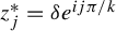
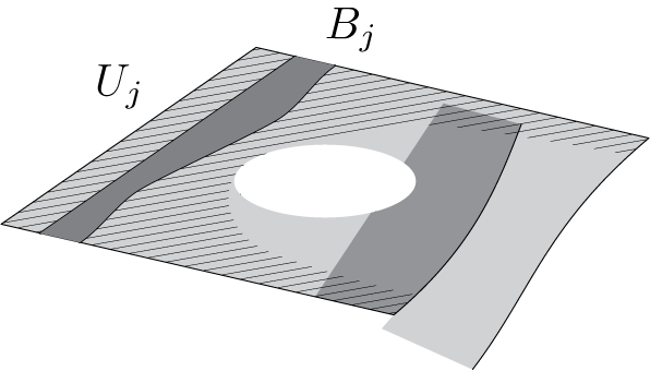
Now we define the sectors in the z-space (see Figure 6). On the Riemann surface of
 $Z_j$
, we write
$Z_j$
, we write
 $G_j$
for the expression of
$G_j$
for the expression of
 $g:= f\circ f$
in the
$g:= f\circ f$
in the
 $Z_j$
-coordinate. Let
$Z_j$
-coordinate. Let
 $z_j^\ast = \delta e^{ij\pi /k}$
for
$z_j^\ast = \delta e^{ij\pi /k}$
for
 $-k\leq j \leq k$
and some small enough
$-k\leq j \leq k$
and some small enough
 $\delta>0$
. Let
$\delta>0$
. Let
 $Z_j^\ast $
be the image of
$Z_j^\ast $
be the image of
 $Z_j(z_j^\ast )$
. We consider a vertical line
$Z_j(z_j^\ast )$
. We consider a vertical line
 $\ell _j$
passing through
$\ell _j$
passing through
 $Z_j^\ast $
and its image
$Z_j^\ast $
and its image
 $G_j(\ell _j)$
. Let
$G_j(\ell _j)$
. Let
 $B_j$
be the domain bounded by
$B_j$
be the domain bounded by
 $\ell _j$
and
$\ell _j$
and
 $G_j(\ell _j)$
and containing
$G_j(\ell _j)$
and containing
 $\ell _j$
and
$\ell _j$
and
 $G_j(\ell _j)$
. The sector in the
$G_j(\ell _j)$
. The sector in the
 $Z_j$
-coordinate is then obtained by
$Z_j$
-coordinate is then obtained by
 $$ \begin{align*}U_j = \{ Z_j\ |\ \textrm{there exists}\ n\in \mathbb{Z},\, G_j^{\circ n}(Z_j) \in B_j\} \end{align*} $$
for
 $-k\leq j \leq k$
(see Figure 7). We see that
$-k\leq j \leq k$
(see Figure 7). We see that
 $U_{-k} = U_k$
, since
$U_{-k} = U_k$
, since
 $Z_k = Z_{-k}$
. The sector
$Z_k = Z_{-k}$
. The sector
 $S_j$
in the z-coordinate is
$S_j$
in the z-coordinate is
 $Z_j^{-1}(U_j)$
(see Figure 6). These sectors are sometimes called Fatou petals. They are described in great detail in [Reference Beardon2], although the authors only considered attractive petals. Note that there are
$Z_j^{-1}(U_j)$
(see Figure 6). These sectors are sometimes called Fatou petals. They are described in great detail in [Reference Beardon2], although the authors only considered attractive petals. Note that there are
 $2k$
petals, with half of them being repulsive (see Figure 8). Also,
$2k$
petals, with half of them being repulsive (see Figure 8). Also,
 $S_k$
and
$S_k$
and
 $S_{-k}$
are the same petal.
$S_{-k}$
are the same petal.
The particular case of
 ${\dot z} = z^4$
. On the right, the sector
${\dot z} = z^4$
. On the right, the sector
 $U_0$
in the
$U_0$
in the
 $Z_0$
-coordinate, obtained from a strip (in dark grey). On the left,
$Z_0$
-coordinate, obtained from a strip (in dark grey). On the left,
 $S_0 = Z^{-1}(U_0)$
the sector in z, with the preimage of the strip (in dark grey).
$S_0 = Z^{-1}(U_0)$
the sector in z, with the preimage of the strip (in dark grey).
A chart
 $U_j$
on the Riemann surface with the vertical strip
$U_j$
on the Riemann surface with the vertical strip
 $B_j$
.
$B_j$
.
Petals for the holomorphic map
 $f\circ f$
. Dynamics inside a repulsive petal on the left. Dynamics inside an attracting petal on the right.
$f\circ f$
. Dynamics inside a repulsive petal on the left. Dynamics inside an attracting petal on the right.
Remark 4.1. Note that
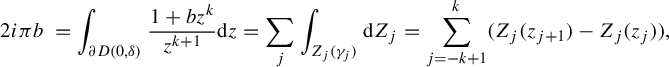 $$ \begin{align*} 2i\pi b\, & = \int_{\partial D(0,\delta)} {1 + bz^k \over z^{k+1}}\mathrm{d} z = \sum_{j}\int_{Z_j(\gamma_j)}\mathrm{d} Z_j = \sum_{j=-k+1}^{k} (Z_{j}(z_{j+1}) - Z_{j}(z_{j})), \end{align*} $$
where
 $\gamma _j$
is an arc of the circle
$\gamma _j$
is an arc of the circle
 $\partial D(0,\delta )$
in
$\partial D(0,\delta )$
in
 $S_j$
, with end points
$S_j$
, with end points
 $z_{j+1}$
and
$z_{j+1}$
and
 $z_{j}$
, where
$z_{j}$
, where
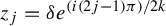 $z_j = \delta e^{(i(2j-1)\pi )/2k}$
. The
$z_j = \delta e^{(i(2j-1)\pi )/2k}$
. The
 $Z_j$
defined as in (12) satisfy this condition.
$Z_j$
defined as in (12) satisfy this condition.
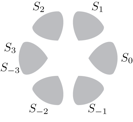
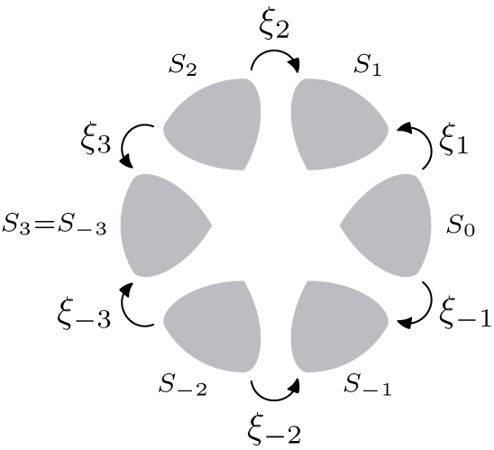
The sectors are ordered as in Figure 9. Note in particular that
 $S_0$
intersects the positive real axis and
$S_0$
intersects the positive real axis and
 $S_k = S_{-k}$
the negative real axis.
$S_k = S_{-k}$
the negative real axis.
Ordering of the sectors for
 $k=3$
.
$k=3$
.
Definition 4.2. The time coordinate is the Riemann surface obtained from the disjoint union of the
 $U_j$
, glued together by the transition functions: the charts are the
$U_j$
, glued together by the transition functions: the charts are the
 $U_j\hookrightarrow \mathbb {C}$
with the diffeomorphism
$U_j\hookrightarrow \mathbb {C}$
with the diffeomorphism
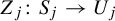 $Z_j\colon S_j \to U_j$
given by
$Z_j\colon S_j \to U_j$
given by
 $$ \begin{align*}Z_j(z) = -{1\over kz^k} + b\log z - {ji\pi b\over k}, \end{align*} $$
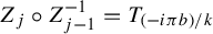
and the transition functions are
 $Z_{j}\circ Z_{j-1}^{-1} = T_{(-i\pi b)/ k}$
for
$Z_{j}\circ Z_{j-1}^{-1} = T_{(-i\pi b)/ k}$
for
 $-k < j \leq k$
, where the composition is defined.
$-k < j \leq k$
, where the composition is defined.
The time coordinate is conformally equivalent to a punctured disk of the origin.
Now we define the complex conjugation on the time coordinate. Note that on a subdomain
 $S_0' \subseteq S_0$
such that
$S_0' \subseteq S_0$
such that
 $\sigma (S_0') = S_0'$
, we have
$\sigma (S_0') = S_0'$
, we have
 $Z_0({\overline z}) = \overline {Z_0(z)}$
. The complex conjugation on the time coordinate is then obtained by analytic continuation on the other charts
$Z_0({\overline z}) = \overline {Z_0(z)}$
. The complex conjugation on the time coordinate is then obtained by analytic continuation on the other charts
 $U_j$
.
$U_j$
.
Proposition 4.3. (Complex conjugation)
For
 $z \in S_j$
, let
$z \in S_j$
, let
 $\ell $
be such that
$\ell $
be such that
 $\sigma (z) = {\overline z} \in S_\ell $
. We define the complex conjugation
$\sigma (z) = {\overline z} \in S_\ell $
. We define the complex conjugation
 $\Sigma $
on the time coordinate in the charts by
$\Sigma $
on the time coordinate in the charts by
 $$ \begin{align*}\Sigma_{\ell,j}\circ Z_j(z) = Z_{\ell}\circ \sigma(z). \end{align*} $$
Then
 $\Sigma $
is well defined and
$\Sigma $
is well defined and
 $\Sigma \circ \Sigma = \mathrm {id}$
.
$\Sigma \circ \Sigma = \mathrm {id}$
.
Proof The proof consists of showing that
 $\Sigma $
is compatible on both charts when
$\Sigma $
is compatible on both charts when
 $Z_j \in U_j \cap U_{j+1}$
or when
$Z_j \in U_j \cap U_{j+1}$
or when
 $\Sigma (Z_j) \in U_\ell \cap U_{\ell \pm 1}$
. It is a simple computation. Note that for a subdomain
$\Sigma (Z_j) \in U_\ell \cap U_{\ell \pm 1}$
. It is a simple computation. Note that for a subdomain
 $S_j'\subset S_j$
such that
$S_j'\subset S_j$
such that
 $\sigma (S_j')\subset S_{-j}$
, then, in the charts, we have
$\sigma (S_j')\subset S_{-j}$
, then, in the charts, we have
 $\Sigma _{-j,j}(Z_j) = \overline {Z_j}$
.
$\Sigma _{-j,j}(Z_j) = \overline {Z_j}$
.
This allows us to talk about the normal form
 $\sigma \circ v^{\scriptscriptstyle {1/2}}$
in the time coordinate. It is the antiholomorphic map
$\sigma \circ v^{\scriptscriptstyle {1/2}}$
in the time coordinate. It is the antiholomorphic map
 $\Sigma \circ {T_{\scriptscriptstyle {1/2}}}$
.
$\Sigma \circ {T_{\scriptscriptstyle {1/2}}}$
.
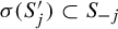
4.2 Fatou coordinates
Let us call the petals of the normal form
 $S_j^v$
. The orbits of the normal form
$S_j^v$
. The orbits of the normal form
 $\sigma \circ v^{\scriptscriptstyle {1/2}}$
jump from
$\sigma \circ v^{\scriptscriptstyle {1/2}}$
jump from
 $S_j^v$
to
$S_j^v$
to
 $S_{-j}^v$
. This means that the dynamics of those two petals is no longer independent, unlike the holomorphic case. See Figure 10.
$S_{-j}^v$
. This means that the dynamics of those two petals is no longer independent, unlike the holomorphic case. See Figure 10.
On the left, an orbit of
 $\sigma \circ v^{\scriptscriptstyle {1/2}}$
in the z-coordinate. The orbit jumps between the sectors
$\sigma \circ v^{\scriptscriptstyle {1/2}}$
in the z-coordinate. The orbit jumps between the sectors
 $S_j^v$
and
$S_j^v$
and
 $S_{-j}^v$
of
$S_{-j}^v$
of
 $\sigma \circ v^{\scriptscriptstyle {1/2}}$
. On the right, the same orbit is represented in the time coordinate; it is the orbit of
$\sigma \circ v^{\scriptscriptstyle {1/2}}$
. On the right, the same orbit is represented in the time coordinate; it is the orbit of
 $\Sigma \circ {T_{\scriptscriptstyle {1/2}}}$
.
$\Sigma \circ {T_{\scriptscriptstyle {1/2}}}$
.
In its prenormalized form f is close to
 $\sigma \circ v^{\scriptscriptstyle {1/2}}$
in the sense that
$\sigma \circ v^{\scriptscriptstyle {1/2}}$
in the sense that
 $|f - \sigma \circ v^{\scriptscriptstyle {1/2}}| = o(|z|^{2k+1})$
. In the following lemma, we prove that it is also true that F and
$|f - \sigma \circ v^{\scriptscriptstyle {1/2}}| = o(|z|^{2k+1})$
. In the following lemma, we prove that it is also true that F and
 $\Sigma \circ {T_{\scriptscriptstyle {1/2}}}$
are close in the time coordinate.
$\Sigma \circ {T_{\scriptscriptstyle {1/2}}}$
are close in the time coordinate.
Lemma 4.4. Let f be in its prenormalized form (7) and let F (respectively
 $\Sigma \circ {T_{\scriptscriptstyle {1/2}}}$
) be the expression of f (respectively
$\Sigma \circ {T_{\scriptscriptstyle {1/2}}}$
) be the expression of f (respectively
 $\sigma \circ v^{\scriptscriptstyle {1/2}}$
) in the time coordinate. On each chart
$\sigma \circ v^{\scriptscriptstyle {1/2}}$
) in the time coordinate. On each chart
 $U_j$
, we have
$U_j$
, we have
 $|F - \Sigma \circ {T_{\scriptscriptstyle {1/2}}}| = O(|Z|^{-1})$
.
$|F - \Sigma \circ {T_{\scriptscriptstyle {1/2}}}| = O(|Z|^{-1})$
.
Proof The proof is similar to that found in [Reference Ilyashenko and Yakovenko6]. Let
 $m(z) = f\circ (\sigma \circ v^{\scriptscriptstyle {1/2}})^{-1}(z) = z + o(z^{2k+1})$
. We see that
$m(z) = f\circ (\sigma \circ v^{\scriptscriptstyle {1/2}})^{-1}(z) = z + o(z^{2k+1})$
. We see that
 $$ \begin{align*} Z_j\circ m(z) &= -{1\over kz^k}(1 + o(z^{2k})) + b\log z + o(z^{2k}) - {ji\pi b\over k}\\ &= Z_j(z) + o(z^k). \end{align*} $$
Since
 $z^kZ_j(z) \to -{(1/k)}$
when
$z^kZ_j(z) \to -{(1/k)}$
when
 $z\to 0$
, and because
$z\to 0$
, and because
 $Z_j$
is invertible and
$Z_j$
is invertible and
 $|Z_j(z)|\to \infty $
when
$|Z_j(z)|\to \infty $
when
 $z\to 0$
, it follows that
$z\to 0$
, it follows that
 $o(z^k)$
is
$o(z^k)$
is
 $O(|Z_j|^{-1})$
when
$O(|Z_j|^{-1})$
when
 $|Z_j|\to \infty $
. Therefore,
$|Z_j|\to \infty $
. Therefore,
 $F\circ (\Sigma \circ {T_{\scriptscriptstyle {1/2}}})^{-1}(Z_j) = Z_j + O(|Z_j|^{-1})$
.
$F\circ (\Sigma \circ {T_{\scriptscriptstyle {1/2}}})^{-1}(Z_j) = Z_j + O(|Z_j|^{-1})$
.
We now present the existence of the Fatou coordinates. Note that Hubbard and Schleicher proved their existence in [Reference Hubbard and Schleicher4, Lemma 2.3] in the codimension-one case for a map with a parabolic periodic orbit of odd period n. We recover their case by considering
 $f^{\circ n}$
. This corresponds for us to a germ of a antiholomorphic parabolic diffeomorphism of codimension one. The proof in higher codimension is in the same spirit with an adaptation, since we need to work with pairs of sectors
$f^{\circ n}$
. This corresponds for us to a germ of a antiholomorphic parabolic diffeomorphism of codimension one. The proof in higher codimension is in the same spirit with an adaptation, since we need to work with pairs of sectors
 $(U_j,U_{-j})$
.
$(U_j,U_{-j})$
.
Proposition 4.5. Let F and
 $\Sigma $
be the expressions of f and
$\Sigma $
be the expressions of f and
 $\sigma $
in the time coordinates, respectively. Recall that
$\sigma $
in the time coordinates, respectively. Recall that
 $U_j = Z_j(S_j)$
. On each
$U_j = Z_j(S_j)$
. On each
 $U_j$
, there exists a holomorphic diffeomorphism
$U_j$
, there exists a holomorphic diffeomorphism
 $\Phi _{j}\colon U_{j} \to \mathbb {C}$
such that
$\Phi _{j}\colon U_{j} \to \mathbb {C}$
such that
 $$ \begin{align} \Phi_j \circ F \circ \Phi_{-j}^{-1} = \Sigma\circ{T_{\scriptscriptstyle{1/2}}} \end{align} $$
whenever the composition is defined.
Moreover, if
 $\widetilde \Phi _{j}$
are other Fatou coordinates, then there exists
$\widetilde \Phi _{j}$
are other Fatou coordinates, then there exists
 $C_j\in \mathbb {C}$
for
$C_j\in \mathbb {C}$
for
 $j=1,\ldots ,k-1$
and
$j=1,\ldots ,k-1$
and
 $C_0,C_k\in \mathbb {R}$
such that
$C_0,C_k\in \mathbb {R}$
such that
 $\Phi _j \circ {\widetilde \Phi _j}^{-1} = T_{C_j}$
and
$\Phi _j \circ {\widetilde \Phi _j}^{-1} = T_{C_j}$
and
 $\Phi _{-j} \circ {\widetilde \Phi _{-j}}^{-1} = T_{\overline C_j}$
for
$\Phi _{-j} \circ {\widetilde \Phi _{-j}}^{-1} = T_{\overline C_j}$
for
 $j\geq 0$
.
$j\geq 0$
.
Proof The proof makes use of the rigidity of the conformal structure of the doubly punctured sphere
 $S^2\setminus \{0,\infty \}$
, as in the proof of the uniqueness in the holomorphic case.
$S^2\setminus \{0,\infty \}$
, as in the proof of the uniqueness in the holomorphic case.
Let
 $\Phi _j$
denote the Fatou coordinate of
$\Phi _j$
denote the Fatou coordinate of
 $f \circ f$
on
$f \circ f$
on
 $U_j$
, that is,
$U_j$
, that is,
 $$ \begin{align*}\Phi_{j} \circ (F \circ F) \circ {(\Phi_{j})}^{-1} = T_1. \end{align*} $$
(We know that it exists, since
 $f \circ f$
is holomorphic, and that it is unique up to left composition with a translation.) In the space of the Fatou coordinate
$f \circ f$
is holomorphic, and that it is unique up to left composition with a translation.) In the space of the Fatou coordinate
 $W_{j} = \Phi _{j}(Z_j)$
, an orbit
$W_{j} = \Phi _{j}(Z_j)$
, an orbit
 $\{ (f\circ f)^{\circ n}(z) \}_n$
corresponds to
$\{ (f\circ f)^{\circ n}(z) \}_n$
corresponds to
 $\{ W_{j} + n \}_n$
. Note also that
$\{ W_{j} + n \}_n$
. Note also that
 $\Phi _j(Z_j) = Z_j + D_j + O(|Z_j|^{-1})$
for some constant
$\Phi _j(Z_j) = Z_j + D_j + O(|Z_j|^{-1})$
for some constant
 $D_j\in \mathbb {C}$
(see [Reference Ilyashenko and Yakovenko6]).
$D_j\in \mathbb {C}$
(see [Reference Ilyashenko and Yakovenko6]).
We first note that each
 $\Phi _j(U_{j})$
contains a vertical strip
$\Phi _j(U_{j})$
contains a vertical strip
 $B_j$
of width one, by construction of the time coordinate
$B_j$
of width one, by construction of the time coordinate
 $U_{j}$
and of the Fatou coordinate. We define
$U_{j}$
and of the Fatou coordinate. We define
 $$ \begin{align*}Q_{j} = \Phi_{- j} \circ F\circ {(\Phi_{j})}^{-1} \qquad\textrm{for }-k\leq j\leq k. \end{align*} $$
Then we see that
 $Q_{j} \circ Q_{-j} = T_1$
, since
$Q_{j} \circ Q_{-j} = T_1$
, since
 $\Phi _{j}$
are Fatou coordinates of
$\Phi _{j}$
are Fatou coordinates of
 $F \circ F$
. It follows that
$F \circ F$
. It follows that
 $Q_{j}$
commutes with
$Q_{j}$
commutes with
 $T_1$
, since
$T_1$
, since
 $$ \begin{align*} T_1 \circ Q_{j} &= (Q_{j} \circ Q_{-j}) \circ Q_{j} \\ &= Q_{j} \circ (Q_{-j} \circ Q_{j}) \\ &= Q_{j} \circ T_1. \end{align*} $$
Indeed,
 $Q_{j}$
represents F in the Fatou coordinates. It is therefore natural that
$Q_{j}$
represents F in the Fatou coordinates. It is therefore natural that
 $Q_{j}$
commutes with
$Q_{j}$
commutes with
 $T_1$
, which represents
$T_1$
, which represents
 $F \circ F$
in the Fatou coordinates.
$F \circ F$
in the Fatou coordinates.
Because
 $Q_j$
is the composition of an antiholomorphic germ by a holomorphic diffeomorphism,
$Q_j$
is the composition of an antiholomorphic germ by a holomorphic diffeomorphism,
 $Q_j$
is antiholomorphic. In particular,
$Q_j$
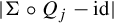
is antiholomorphic. In particular,
 $\Sigma \circ Q_j$
is holomorphic, and
$\Sigma \circ Q_j$
is holomorphic, and
 $\Sigma \circ Q_{j} - \mathrm {id}$
is
$\Sigma \circ Q_{j} - \mathrm {id}$
is
 $1$
-periodic and holomorphic, so it has a Fourier expansion
$1$
-periodic and holomorphic, so it has a Fourier expansion
 $$ \begin{align*}\Sigma\circ Q_{j}(W_{j}) - W_{j} = \sum_{n=-\infty}^\infty c_{n,j} e^{2i\pi n W_{j}}. \end{align*} $$
Moreover, by Lemma 4.4, we have
 $\Sigma \circ Q_j(W) = W + M_j + O(|W|^{-1})$
, where
$\Sigma \circ Q_j(W) = W + M_j + O(|W|^{-1})$
, where
 $M_j\in \mathbb {C}$
is a constant. Therefore,
$M_j\in \mathbb {C}$
is a constant. Therefore,
 $|\Sigma \circ Q_j - \mathrm {id}|$
is bounded when
$|\Sigma \circ Q_j - \mathrm {id}|$
is bounded when
 $|W| \to \infty $
, so we must have
$|W| \to \infty $
, so we must have
 $c_{n,j} = 0$
for
$c_{n,j} = 0$
for
 $n\in \mathbb {Z}^\ast $
.
$n\in \mathbb {Z}^\ast $
.
We conclude that
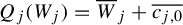 $Q_{j}(W_j) = \overline W_j + \overline {c_{j,0}}$
. Since
$Q_{j}(W_j) = \overline W_j + \overline {c_{j,0}}$
. Since
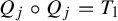 $Q_j\circ Q_j = T_1$
, it follows that
$Q_j\circ Q_j = T_1$
, it follows that
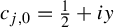 $c_{j,0} = {\tfrac 12} + iy$
. We then adjust all the
$c_{j,0} = {\tfrac 12} + iy$
. We then adjust all the
 $\textrm{Im}\kern2pt c_{j,0}$
to 0 by choosing the appropriate Fatou coordinates (that is, composing them with a translation).
$\textrm{Im}\kern2pt c_{j,0}$
to 0 by choosing the appropriate Fatou coordinates (that is, composing them with a translation).
The uniqueness comes from a combination of the uniqueness of the Fatou coordinates for the holomorphic
 $f \circ f$
and having to preserve the constants
$f \circ f$
and having to preserve the constants
 $c_{j,0} = \frac {1}{2}$
.
$c_{j,0} = \frac {1}{2}$
.
5 Modulus of analytic classification
If two antiholomorphic parabolic germs are analytically conjugate, then they have the same space of orbits. The space of orbits of an antiholomorphic parabolic germ f is a quotient of the set of orbits of the associated holomorphic parabolic germ
 $g = f \circ f$
. Hence, we start by describing the space of orbits of g; on a Fatou coordinate, it is the quotient by
$g = f \circ f$
. Hence, we start by describing the space of orbits of g; on a Fatou coordinate, it is the quotient by
 $T_1$
, which is a bi-infinite cylinder. We also need to identify some orbits represented in two different Fatou coordinates. This is done by means of the transition maps (the horn maps of Écalle).
$T_1$
, which is a bi-infinite cylinder. We also need to identify some orbits represented in two different Fatou coordinates. This is done by means of the transition maps (the horn maps of Écalle).
We will describe the space of orbits of f in §6.1 and classify the antiholomorphic germs in §6.3. To do both of these, we will need the transition functions, which will form an analytic invariant.
The transition functions we describe here are the same as for the holomorphic case. We will introduce what we need here; all the details are found in [Reference Ilyashenko5] or [Reference Ilyashenko and Yakovenko6].
In the time coordinate, if
 $U_j$
is a repelling (respectively attractive) petal, then
$U_j$
is a repelling (respectively attractive) petal, then
 $U_j$
and
$U_j$
and
 $T_{i\pi b/k}(U_{j+1})$
intersect on a domain containing an upper half-plane (respectively a lower half-plane); see Figure 11. (Recall that
$T_{i\pi b/k}(U_{j+1})$
intersect on a domain containing an upper half-plane (respectively a lower half-plane); see Figure 11. (Recall that
 $T_{-i\pi b/k}$
is a transition function on a Riemann surface of the time coordinate; see Definition 4.2.) We can compare the Fatou coordinates
$T_{-i\pi b/k}$
is a transition function on a Riemann surface of the time coordinate; see Definition 4.2.) We can compare the Fatou coordinates
 $\Phi _j$
and
$\Phi _j$
and
 $\Phi _{j+1}$
by looking at
$\Phi _{j+1}$
by looking at
respectively
where
 $V_j = \Phi _j(U_j)$
for all j. This yields a diffeomorphism defined on a domain of
$V_j = \Phi _j(U_j)$
for all j. This yields a diffeomorphism defined on a domain of
 $V_{j}$
(respectively
$V_{j}$
(respectively
 $V_{j+1}$
) containing an upper half-plane (respectively lower half-plane) with its image in
$V_{j+1}$
) containing an upper half-plane (respectively lower half-plane) with its image in
 $V_{j+1}$
(respectively
$V_{j+1}$
(respectively
 $V_j$
) also containing some upper half-plane (respectively lower half-plane).
$V_j$
) also containing some upper half-plane (respectively lower half-plane).
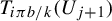
Charts
 $U_{j-1}$
and
$U_{j-1}$
and
 $U_j$
on the time coordinate. They intersect in a region containing (in this case) an upper half-plane.
$U_j$
on the time coordinate. They intersect in a region containing (in this case) an upper half-plane.
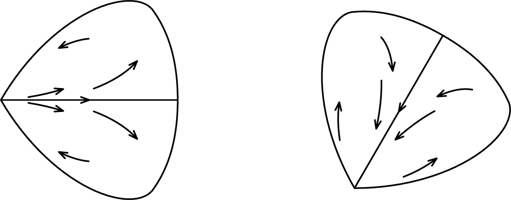
Notice the order of the composition for
 $\Psi _j$
: we choose the convention that these functions will go from a repulsive petal to an attractive petal. Figure 12 is an illustration of the direction of the arrows in the z-coordinate for
$\Psi _j$
: we choose the convention that these functions will go from a repulsive petal to an attractive petal. Figure 12 is an illustration of the direction of the arrows in the z-coordinate for
 $k=3$
, where
$k=3$
, where
 $\xi _j$
is the expression of
$\xi _j$
is the expression of
 $\Psi _j$
in the z-coordinate.
$\Psi _j$
in the z-coordinate.
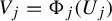
Direction of the transition functions
 $\{\xi _j\}_j$
represented in the z-coordinates.
$\{\xi _j\}_j$
represented in the z-coordinates.
Definition 5.1. Let
 $\Phi _j$
be a Fatou coordinate of f on
$\Phi _j$
be a Fatou coordinate of f on
 $U_j$
. The transition functions (equivalent to the Écalle horn maps) of f are the
$U_j$
. The transition functions (equivalent to the Écalle horn maps) of f are the
 $2k$
functions
$2k$
functions
 $\Psi _j$
for
$\Psi _j$
for
 $j=1,\ldots ,k$
and
$j=1,\ldots ,k$
and
 $j=-1,\ldots ,-k$
obtained by
$j=-1,\ldots ,-k$
obtained by
 $$ \begin{align} \Psi_j = \begin{cases} \Phi_{j} \circ T_{\scriptscriptstyle-\mathop{\mathrm{sgn}}\nolimits(j){(i\pi b/k)}} \circ \Phi_{j-\mathop{\mathrm{sgn}}\nolimits(j)}^{-1} & \textrm{for }j \textrm{ odd},\\[3pt] \Phi_{j-\mathop{\mathrm{sgn}}\nolimits(j)} \circ T_{\scriptscriptstyle\mathop{\mathrm{sgn}}\nolimits(j){(i\pi b/k)}}\circ \Phi_{j}^{-1} &\textrm{for }j \textrm{ even}, \end{cases} \end{align} $$
where the composition is defined. Here,
 $\mathop {\mathrm {sgn}}\nolimits (j)$
is the sign of j.
$\mathop {\mathrm {sgn}}\nolimits (j)$
is the sign of j.
By the uniqueness of Proposition 4.5, we may change
 $\Phi _{\pm j}$
by
$\Phi _{\pm j}$
by
 $T_{C_j} \circ \Phi _j$
and
$T_{C_j} \circ \Phi _j$
and
 $T_{\overline C_j} \circ \Phi _{-j}$
for some
$T_{\overline C_j} \circ \Phi _{-j}$
for some
 $C_j\in \mathbb {C}$
for
$C_j\in \mathbb {C}$
for
 $j=1,\ldots ,k-1$
, or
$j=1,\ldots ,k-1$
, or
 $\Phi _{j}$
by
$\Phi _{j}$
by
 $T_{R_j} \circ \Phi _j$
for some
$T_{R_j} \circ \Phi _j$
for some
 $R_j\in \mathbb {R}$
for
$R_j\in \mathbb {R}$
for
 $j=0,k$
. This will yield another set of
$j=0,k$
. This will yield another set of
 $2k$
transition functions. We will identify together these different possible choices of transition functions at the end of this section.
$2k$
transition functions. We will identify together these different possible choices of transition functions at the end of this section.
The following proposition is the first step towards the geometric invariant. The transition functions allow us to describe the space of orbits of F and
 $F\circ F$
.
$F\circ F$
.
Proposition 5.2. Let
 $(\Psi _{-k},\ldots ,\Psi _{-1},\Psi _1,\ldots ,\Psi _k)$
be transition functions of f. They satisfy the equation
$(\Psi _{-k},\ldots ,\Psi _{-1},\Psi _1,\ldots ,\Psi _k)$
be transition functions of f. They satisfy the equation
 $$ \begin{align} \Sigma \circ {T_{\scriptscriptstyle{1/2}}} \circ \Psi_j = \Psi_{-j} \circ \Sigma \circ {T_{\scriptscriptstyle{1/2}}}. \end{align} $$
In particular, they are transition functions of
 $f\circ f$
and satisfy
$f\circ f$
and satisfy
 $$ \begin{align} T_1 \circ \Psi_j = \Psi_j \circ T_1. \end{align} $$
Proof The proof is identical to the holomorphic case; it follows from the definition of
 $\Psi _j$
and (13).
$\Psi _j$
and (13).
Equation (15) says that the orbits of
 $\Sigma \circ {T_{\scriptscriptstyle {1/2}}}$
in one Fatou coordinate are sent by the
$\Sigma \circ {T_{\scriptscriptstyle {1/2}}}$
in one Fatou coordinate are sent by the
 $\Psi _j$
on the orbits of
$\Psi _j$
on the orbits of
 $\Sigma \circ {T_{\scriptscriptstyle {1/2}}}$
in another Fatou coordinate. In those coordinates, the orbits of
$\Sigma \circ {T_{\scriptscriptstyle {1/2}}}$
in another Fatou coordinate. In those coordinates, the orbits of
 $\Sigma \circ {T_{\scriptscriptstyle {1/2}}}$
correspond to those of f. Therefore, the transition functions allow us to identify the same orbits of f in different coordinates.
$\Sigma \circ {T_{\scriptscriptstyle {1/2}}}$
correspond to those of f. Therefore, the transition functions allow us to identify the same orbits of f in different coordinates.
We can rewrite equation (15) as
 $$ \begin{align} \Psi_{-j} = \Sigma\circ {T_{\scriptscriptstyle{1/2}}} \circ \Psi_j \circ \Sigma \circ T_{\scriptscriptstyle{-{1/2}}}, \end{align} $$
so that
 $\Psi _{-j}$
is determined by
$\Psi _{-j}$
is determined by
 $\Psi _j$
. Thus, we only need half of the transition functions of f to determine all of them. For the rest of the paper, we will work with
$\Psi _j$
. Thus, we only need half of the transition functions of f to determine all of them. For the rest of the paper, we will work with
 $\Psi _1, \ldots ,\Psi _k$
, knowing that
$\Psi _1, \ldots ,\Psi _k$
, knowing that
 $\Psi _{-1},\ldots ,\Psi _{-k}$
are obtained from equation (17).
$\Psi _{-1},\ldots ,\Psi _{-k}$
are obtained from equation (17).
The transition functions in the holomorphic case are well known and their properties are described by Ilyashenko [Reference Ilyashenko5]. Because the transition functions of f are also those of
 $f\circ f$
, they share the properties which we describe now.
$f\circ f$
, they share the properties which we describe now.
Each
 $\Psi _j$
satisfies equation (16); it follows that
$\Psi _j$
satisfies equation (16); it follows that
 $\Psi _j - \mathrm {id}$
is 1-periodic and has a Fourier expansion
$\Psi _j - \mathrm {id}$
is 1-periodic and has a Fourier expansion
 $$ \begin{align} \begin{aligned} \Psi_j(W) - W &= c_j + \sum_{n=1}^\infty c_{n,j} e^{2i\pi nW} \quad\ \textrm{for }j> 0\textrm{ odd,}\\ \Psi_j(W) - W &= c_j + \sum_{n=-1}^{-\infty} c_{n,j} e^{2i\pi nW} \quad\ \textrm{for }j > 0\textrm{ even.} \end{aligned} \end{align} $$
In particular, we see that
 $|\Psi _j -\mathrm {id} - c_j|$
is exponentially decreasing when
$|\Psi _j -\mathrm {id} - c_j|$
is exponentially decreasing when
 $\textrm{Im}\kern2pt W \to \infty $
and j is odd (respectively
$\textrm{Im}\kern2pt W \to \infty $
and j is odd (respectively
 $\textrm{Im}\kern2pt W \to -\infty $
and j is even).
$\textrm{Im}\kern2pt W \to -\infty $
and j is even).
Since the Fatou coordinates are not unique, we may change them and obtain new transition functions. This will change the constants
 $c_j$
and
$c_j$
and
 $c_{n,j}$
, but the following alternating sum will always be preserved:
$c_{n,j}$
, but the following alternating sum will always be preserved:
 $$ \begin{align} \begin{aligned} (-1)^{k-1} c_{-k} &+ (-1)^{k-2} c_{-k+1} \pm \cdots - c_{-2} + c_{-1}\\ &{} - c_1 + c_2 - \cdots + (-1)^{k-1} c_{k-1} + (-1)^{k} c_{k} = 2i\pi b. \end{aligned} \end{align} $$
We successively change
 $\Phi _{1}$
by
$\Phi _{1}$
by
 $T_{-c_1 - {(i\pi b)/k}}\circ \Phi _1$
,
$T_{-c_1 - {(i\pi b)/k}}\circ \Phi _1$
,
 $\Phi _2$
by
$\Phi _2$
by
 $T_{-c_1+c_2-{(2i\pi b)/k}}$
,
$T_{-c_1+c_2-{(2i\pi b)/k}}$
,
 $\Phi _3$
by
$\Phi _3$
by
 $T_{-c_1+c_2-c_3-{(3i\pi b)/k}}\circ \Phi _3$
, and so on. The constant terms of the new transition functions will satisfy
$T_{-c_1+c_2-c_3-{(3i\pi b)/k}}\circ \Phi _3$
, and so on. The constant terms of the new transition functions will satisfy
 $$ \begin{align} c_j = \begin{cases} \displaystyle-{i\pi b \over k} & \textrm{for }j>0\textrm{ odd,}\\ \displaystyle\phantom{-}{i\pi b \over k} & \textrm{for }j>0 \textrm{ even.} \end{cases} \end{align} $$
for
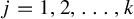 $j=1,2,\ldots ,k$
. Note that, together with equation (17), the constant terms
$j=1,2,\ldots ,k$
. Note that, together with equation (17), the constant terms
 $c_j$
for
$c_j$
for
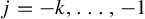 $j=-k,\ldots ,-1$
are given by
$j=-k,\ldots ,-1$
are given by
 $c_j = \overline {c_{-j}}$
.
$c_j = \overline {c_{-j}}$
.
Definition 5.3. (Normalized transition functions)
The transition functions
 $(\Psi _1,\ldots ,\Psi _k)$
are said to be normalized if the constant terms
$(\Psi _1,\ldots ,\Psi _k)$
are said to be normalized if the constant terms
 $c_j$
of equation (18) satisfy (20) for
$c_j$
of equation (18) satisfy (20) for
 $j=1,2,\ldots ,k$
.
$j=1,2,\ldots ,k$
.
Even when normalized, the transition functions are not uniquely determined. There is still a remaining degree of freedom: we may change the source and target spaces of each
 $\Psi _j$
by the same translation
$\Psi _j$
by the same translation
 $T_C$
with
$T_C$
with
 $C \in \mathbb {R}$
.
$C \in \mathbb {R}$
.
In the case of even codimension, if f is prenormalized, then
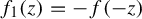 $f_1(z)=-f(-z)$
is also prenormalized, and f and
$f_1(z)=-f(-z)$
is also prenormalized, and f and
 $f_1$
are conjugate. Hence, we will need to identify their moduli.
$f_1$
are conjugate. Hence, we will need to identify their moduli.
Definition 5.4. (Modulus of classification)
We define the equivalence relation
 $\sim $
on normalized transition functions of the form (18) by
$\sim $
on normalized transition functions of the form (18) by
 $$ \begin{align} (\Psi_1,\ldots,\Psi_k)\sim(\Psi_1',\ldots,\Psi_k') \Leftrightarrow \textrm{there exists}\ C\in \mathbb{R}, \Psi_j = T_C \circ \Psi_j' \circ T_{-C}. \end{align} $$
The modulus of classification of f of codimension k (and of positive type when k is even) (see Definition 2.6) is defined by the triple
 $(k,b,[\Psi _1,\ldots ,\Psi _k])$
, where k is the codimension (Definition 2.5), b is the formal invariant (Definition 2.9), and
$(k,b,[\Psi _1,\ldots ,\Psi _k])$
, where k is the codimension (Definition 2.5), b is the formal invariant (Definition 2.9), and
 $[\Psi _1,\ldots ,\Psi _k]$
is the equivalence class of normalized transition functions of f (Definitions 5.1 and 5.3), where the equivalence class is defined according to the following two cases.
$[\Psi _1,\ldots ,\Psi _k]$
is the equivalence class of normalized transition functions of f (Definitions 5.1 and 5.3), where the equivalence class is defined according to the following two cases.
-
(1) If k is odd, then
$[\Psi _1,\ldots ,\Psi _k]$
is the equivalence class under the relation (21). -
(2) If k is even, then
$[\Psi _1,\ldots ,\Psi _k]$
is the equivalence class under the relation (21) and the additional relation (22)
$$ \begin{align} \hspace{-0.8pc}(\Psi_1,\ldots,\Psi_k)\cong (\Psi_1',\ldots,\Psi_k') \iff \Psi_j' = \Sigma\circ {T_{\scriptscriptstyle{1/2}}} \circ \Psi_{k-j+1} \circ \Sigma\circ T_{\scriptscriptstyle{-{1/2}}}.\quad \end{align} $$


This equivalence class is called the analytic invariant.
5.1 Remarks on the Écalle–Voronin modulus
In the holomorphic case, the modulus of classification is known as the Écalle–Voronin modulus (see [Reference Ilyashenko5, Reference Ilyashenko and Yakovenko6]). For any holomorphic parabolic germ g (not necessarily of the form
 $g = f\circ f$
), we can obtain its Écalle–Voronin modulus in the same way as described above, but without equation (15), so that the
$g = f\circ f$
), we can obtain its Écalle–Voronin modulus in the same way as described above, but without equation (15), so that the
 $2k$
transition functions are needed. There are
$2k$
transition functions are needed. There are
 $2k$
degrees of freedom, so we normalize the transition functions by choosing the constant terms as in (20) and with
$2k$
degrees of freedom, so we normalize the transition functions by choosing the constant terms as in (20) and with
 $c_{-j}=-c_j$
; the remaining degree of freedom is a translation in every Fatou coordinate by a constant
$c_{-j}=-c_j$
; the remaining degree of freedom is a translation in every Fatou coordinate by a constant
 $C\in \mathbb {C}$
. Therefore, we quotient by the equivalence relation
$C\in \mathbb {C}$
. Therefore, we quotient by the equivalence relation
 $$ \begin{align} (\Psi_{-k},\ldots,\Psi_{-1},\Psi_1,\ldots,\Psi_k) &\sim_{\mathbb{C}}(\Psi_{-k}',\ldots,\Psi_{-1}',\Psi_1',\ldots,\Psi_k')\nonumber\\ &\ \Leftrightarrow \textrm{there exists}\ C\in \mathbb{C}, \Psi_j = T_C \circ \Psi_j' \circ T_{-C}\nonumber\\ &\quad\quad\textrm{for}\ j\in\{-k,\ldots,-1\}\cup\{1,\ldots,k\}. \end{align} $$
We also quotient by the action of the rotations of order k. If we denote the indices
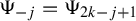 $\Psi _{-j}=\Psi _{2k-j+1}$
for
$\Psi _{-j}=\Psi _{2k-j+1}$
for
 $j=1,\ldots , k$
, then we have the identification
$j=1,\ldots , k$
, then we have the identification
 $$ \begin{align} (\Psi_{k+1},\ldots,\Psi_{2k},&\Psi_1,\ldots,\Psi_k) \sim (\Psi_{k+1+2m}',\ldots,\Psi_{2k+2m}',\Psi_{1+2m}',\ldots,\Psi_{k+2m}')\nonumber\\ &\qquad\qquad\qquad\quad\textrm{for }m=0,\ldots,k-1,\end{align} $$
where the indices are mod
 $2k$
. We will denote the equivalence class of both of these identifications by
$2k$
. We will denote the equivalence class of both of these identifications by
 $[\Psi _{-k},\ldots ,\Psi _{-1}, \Psi _1,\ldots ,\Psi _k]$
. The modulus of g is then
$[\Psi _{-k},\ldots ,\Psi _{-1}, \Psi _1,\ldots ,\Psi _k]$
. The modulus of g is then
 $(k,b,[\Psi _{-k},\ldots ,\Psi _{-1}, \Psi _1,\ldots ,\Psi _k])$
.
$(k,b,[\Psi _{-k},\ldots ,\Psi _{-1}, \Psi _1,\ldots ,\Psi _k])$
.
We describe the link between the Écalle–Voronin modulus of g and the modulus of classification of an antiholomorphic parabolic germ f of positive type such that
 $g = f\circ f$
when such a f exists. The symmetry axis of f appears along one of the ‘symmetry axes’ of g of the form
$g = f\circ f$
when such a f exists. The symmetry axis of f appears along one of the ‘symmetry axes’ of g of the form
 $e^{2i\ell \pi / k}\mathbb {R}$
,
$e^{2i\ell \pi / k}\mathbb {R}$
,
 $\ell = 0,\ldots ,k-1$
. (Note that for k even,
$\ell = 0,\ldots ,k-1$
. (Note that for k even,
 $e^{2i\ell \pi / k}\mathbb {R}$
and
$e^{2i\ell \pi / k}\mathbb {R}$
and
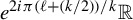 $e^{2i\pi (\ell + (k/2))/k}\mathbb {R}$
are the same axis, so there are
$e^{2i\pi (\ell + (k/2))/k}\mathbb {R}$
are the same axis, so there are
 $k/2$
possible axes for f of positive type and
$k/2$
possible axes for f of positive type and
 $k/2$
for f of negative type.) Therefore, we associate to the analytic invariant of g the regular k-gon with the k symmetry axes
$k/2$
for f of negative type.) Therefore, we associate to the analytic invariant of g the regular k-gon with the k symmetry axes
 $e^{i\ell \pi / k}\mathbb {R}$
,
$e^{i\ell \pi / k}\mathbb {R}$
,
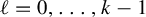 $\ell =0,\ldots ,k-1$
, in the following way. Divide the k-gon by its k symmetry axes to produce
$\ell =0,\ldots ,k-1$
, in the following way. Divide the k-gon by its k symmetry axes to produce
 $2k$
sectors in the k-gon; then, starting with the sector above the horizontal line on the right-hand side, we identify this sector with
$2k$
sectors in the k-gon; then, starting with the sector above the horizontal line on the right-hand side, we identify this sector with
 $\Psi _1$
and, going anticlockwise, we associate
$\Psi _1$
and, going anticlockwise, we associate
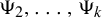 $\Psi _2,\ldots , \Psi _k$
,
$\Psi _2,\ldots , \Psi _k$
,
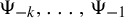 $\Psi _{-k},\ldots ,\Psi _{-1}$
to the subsequent sectors, as in Figures 13(a) and 14(a). The dihedral group
$\Psi _{-k},\ldots ,\Psi _{-1}$
to the subsequent sectors, as in Figures 13(a) and 14(a). The dihedral group
 $D_{2k}$
of symmetries of the k-gon acts on the sectors of the k-gon. It contains k rotations of order dividing k and k reflections. The action is defined for an element
$D_{2k}$
of symmetries of the k-gon acts on the sectors of the k-gon. It contains k rotations of order dividing k and k reflections. The action is defined for an element
 $u\in D_{2k}$
by mapping a sector to its image by the linear application represented by u (a rotation or a reflection).
$u\in D_{2k}$
by mapping a sector to its image by the linear application represented by u (a rotation or a reflection).
Definition 5.5. Let
 $u\in D_{2k}$
and let
$u\in D_{2k}$
and let
 $\Delta _j$
be the sector of the k-gon associated with
$\Delta _j$
be the sector of the k-gon associated with
 $\Psi _j$
. The action of u on the sectors of the regular k-gon defines a permutation on
$\Psi _j$
. The action of u on the sectors of the regular k-gon defines a permutation on
 $\{-k,\ldots ,-1,1,\ldots ,k\}$
, also denoted u by abuse of notation, defined so that
$\{-k,\ldots ,-1,1,\ldots ,k\}$
, also denoted u by abuse of notation, defined so that
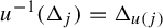 $u^{-1}(\Delta _j) = \Delta _{u(j)}$
(see Figure 13 for
$u^{-1}(\Delta _j) = \Delta _{u(j)}$
(see Figure 13 for
 $k=5$
and Figure 14 for
$k=5$
and Figure 14 for
 $k=6$
).
$k=6$
).
Codimension five. The permutations of indices induced by s and r are
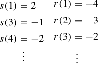 $ \begin {aligned} s(1) &= 2\\ s(3) &= -1\\ s(4) &= -2\\[-4pt] &\:\,\vdots \end {aligned} \quad \begin {aligned} r(1) &= -4\\ r(2) &= -3\\ r(3) &= -2\\ &\:\:\vdots \end {aligned} $
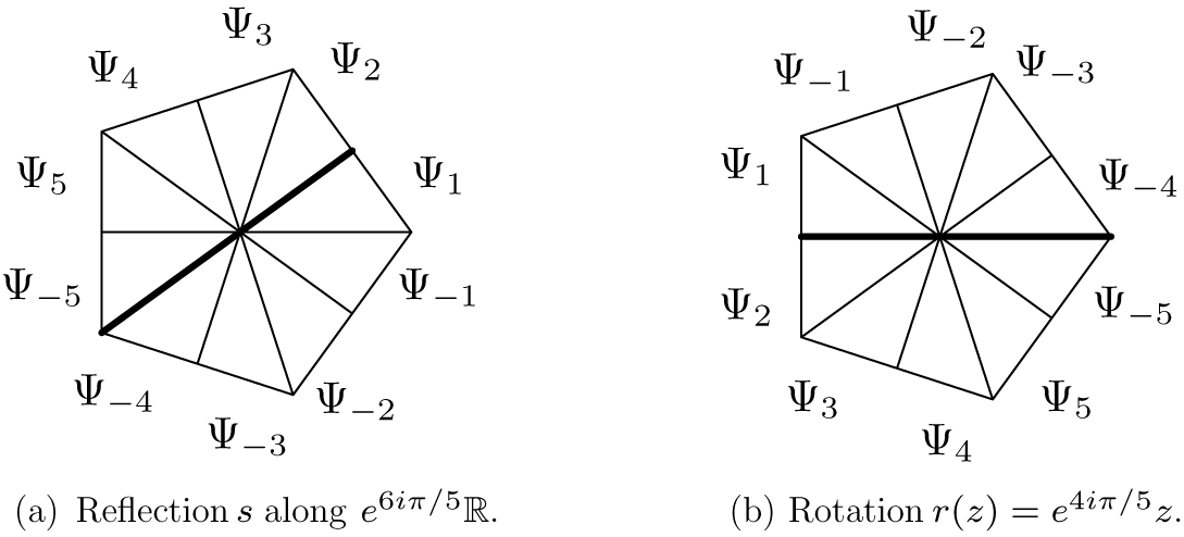
Codimension six. Symmetry axis of f along
 $e^{4i\pi /6}\mathbb {R}$
. The permutations of indices s,
$e^{4i\pi /6}\mathbb {R}$
. The permutations of indices s,
 $r_1$
and
$r_1$
and
 $r_2$
are
$r_2$
are
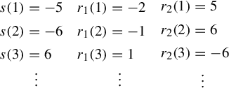 $\begin {aligned} s(1) &= -5\\ s(2) &= -6\\ s(3) &= 6\\[-4pt] &\:\:\,\vdots \end {aligned}\quad \begin {aligned} r_1(1) &= -2\\ r_1(2) &= -1\\ r_1(3) &= 1\\[-4pt] &\:\:\,\vdots \end {aligned}\quad \begin {aligned} r_2(1) &= 5\\ r_2(2) &= 6\\ r_2(3) &= -6\\[-2pt] &\:\:\,\vdots \end {aligned} $
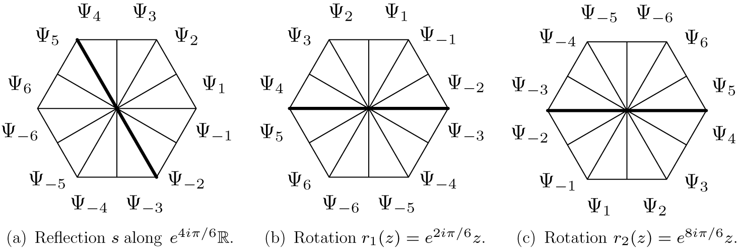
Proposition 5.6. Let g be a holomorphic parabolic germ with modulus
 $(k,b,[\Psi _{-k},\ldots , \Psi _{-1},\Psi _1,\ldots ,\Psi _k])$
. Suppose that f is an antiholomorphic parabolic germ of positive type with the symmetry along
$(k,b,[\Psi _{-k},\ldots , \Psi _{-1},\Psi _1,\ldots ,\Psi _k])$
. Suppose that f is an antiholomorphic parabolic germ of positive type with the symmetry along
 $e^{2i\pi \ell /k}\mathbb {R}$
for some
$e^{2i\pi \ell /k}\mathbb {R}$
for some
 $\ell \in \{0,1,\ldots ,k-1\}$
. Let r be the rotation
$\ell \in \{0,1,\ldots ,k-1\}$
. Let r be the rotation
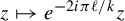 $z\mapsto e^{-2i\pi \ell / k}z$
and s the reflection with respect to
$z\mapsto e^{-2i\pi \ell / k}z$
and s the reflection with respect to
 $e^{2i\pi \ell /k}\mathbb {R}$
. If
$e^{2i\pi \ell /k}\mathbb {R}$
. If
 $f\circ f = g$
, then there exists a representative
$f\circ f = g$
, then there exists a representative
 $(\Psi _{-k}',\ldots ,\Psi _{-1}',\Psi _1',\ldots ,\Psi _k')$
of the analytic invariant of g such that
$(\Psi _{-k}',\ldots ,\Psi _{-1}',\Psi _1',\ldots ,\Psi _k')$
of the analytic invariant of g such that
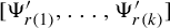 $[\Psi _{r(1)}',\ldots ,\Psi _{r(k)}']$
is the analytic invariant of f and satisfies
$[\Psi _{r(1)}',\ldots ,\Psi _{r(k)}']$
is the analytic invariant of f and satisfies
 $$ \begin{align} \Psi_{r(j)}' \circ \Sigma\circ{T_{\scriptscriptstyle{1/2}}} = \Sigma\circ{T_{\scriptscriptstyle{1/2}}} \circ \Psi_{r(-j)}' \end{align} $$
or, equivalently,
 $$ \begin{align} \Psi_{j}' \circ \Sigma\circ{T_{\scriptscriptstyle{1/2}}} = \Sigma\circ{T_{\scriptscriptstyle{1/2}}} \circ \Psi_{s(j)}'. \end{align} $$
Proof Let
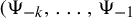 $(\Psi _{-k},\ldots ,\Psi _{-1}$
,
$(\Psi _{-k},\ldots ,\Psi _{-1}$
,
 $\Psi _1,\ldots ,\Psi _k)$
be a representative of the analytic invariant of g. Since r is a rotation with an order dividing k, it is an element of
$\Psi _1,\ldots ,\Psi _k)$
be a representative of the analytic invariant of g. Since r is a rotation with an order dividing k, it is an element of
 $D_{2k}$
. It rotates the coordinate so that the symmetry axis corresponds to the real axis with a repulsive petal on the side of
$D_{2k}$
. It rotates the coordinate so that the symmetry axis corresponds to the real axis with a repulsive petal on the side of
 $\mathbb {R}^+$
(this is the case because f is of positive type). The representative of the modulus of g is permuted:
$\mathbb {R}^+$
(this is the case because f is of positive type). The representative of the modulus of g is permuted:
 $(\Psi _{r(-k)},\ldots ,\Psi _{r(-1)},\Psi _{r(1)},\ldots ,\Psi _{r(k)})$
as in (24); it now has an equivalent representative
$(\Psi _{r(-k)},\ldots ,\Psi _{r(-1)},\Psi _{r(1)},\ldots ,\Psi _{r(k)})$
as in (24); it now has an equivalent representative
 $(\Psi _{r(-k)}',\ldots ,\Psi _{r(-1)}',\Psi _{r(1)}',\ldots ,\Psi _{r(k)}')$
under relation (23) obtained from the Fatou coordinates of f, so that it satisfies
$(\Psi _{r(-k)}',\ldots ,\Psi _{r(-1)}',\Psi _{r(1)}',\ldots ,\Psi _{r(k)}')$
under relation (23) obtained from the Fatou coordinates of f, so that it satisfies
 $$ \begin{align*}\Psi_{r(j)}'\circ \Sigma\circ{T_{\scriptscriptstyle{1/2}}} = \Sigma\circ{T_{\scriptscriptstyle{1/2}}} \circ \Psi_{r(-j)}'. \end{align*} $$
Equation (26) follows from
 $r^{-1} sr = \sigma $
, where
$r^{-1} sr = \sigma $
, where
 $\sigma $
is the usual complex conjugation. Indeed, on the indices, we have
$\sigma $
is the usual complex conjugation. Indeed, on the indices, we have
 $r(-j) = r\sigma (j)$
and, substituting
$r(-j) = r\sigma (j)$
and, substituting
 $\ell = r(j)$
, the previous equation becomes
$\ell = r(j)$
, the previous equation becomes
 $$ \begin{align*}\Psi_\ell'\circ \Sigma\circ{T_{\scriptscriptstyle{1/2}}} = \Sigma\circ{T_{\scriptscriptstyle{1/2}}} \circ \Psi_{s(\ell)}'. \\[-36pt] \end{align*} $$
Definition 5.7. A reflection
 $s\in D_{2k}$
is a symmetry of the analytic modulus of g if it satisfies (26). For each reflection
$s\in D_{2k}$
is a symmetry of the analytic modulus of g if it satisfies (26). For each reflection
 $s_1,\ldots ,s_n$
of the analytic invariant, we define
$s_1,\ldots ,s_n$
of the analytic invariant, we define
 $H = \langle s_1,\ldots ,s_n\rangle $
to be the group of symmetries of the modulus.
$H = \langle s_1,\ldots ,s_n\rangle $
to be the group of symmetries of the modulus.
Remark 5.8. A group H as in the definition is always a dihedral group of order at most
 $2k$
(see [Reference Grove and Benson3, §2.2]). If it is non-trivial, it contains a rotation of order at most k. The group of symmetries of a modulus is related to the number of distinct antiholomorphic square roots of g. This problem is addressed in §7.2.
$2k$
(see [Reference Grove and Benson3, §2.2]). If it is non-trivial, it contains a rotation of order at most k. The group of symmetries of a modulus is related to the number of distinct antiholomorphic square roots of g. This problem is addressed in §7.2.
The analogous result of Proposition 5.6 for the case of negative type can be obtained by studying the inverse of a holomorphic parabolic germ g. The following proposition is probably well known, but we could not find it in the literature, so the proof is included.
Proposition 5.9. Let g be a holomorphic parabolic germ. Let the modulus of g be
 $(k,b,[\Psi _{-k},\ldots ,\Psi _{-1},\Psi _1,\ldots ,\Psi _k])$
. Then the modulus of
$(k,b,[\Psi _{-k},\ldots ,\Psi _{-1},\Psi _1,\ldots ,\Psi _k])$
. Then the modulus of
 $g^{-1}$
is given by
$g^{-1}$
is given by
 $$ \begin{align}\let\widetilde=\widetilde (k,-b, [\widetilde\Psi_{-k},\ldots,\widetilde\Psi_{-1}, \widetilde\Psi_1, \ldots, \widetilde\Psi_{k}]), \end{align} $$
where
 $\widetilde \Psi _j$
stands for
$\widetilde \Psi _j$
stands for
 $L_{-1}\circ \Psi _{r_1^{-1}(j)}^{-1}\circ L_{-1}$
, with
$L_{-1}\circ \Psi _{r_1^{-1}(j)}^{-1}\circ L_{-1}$
, with
 $L_{-1}\colon Y\mapsto -Y$
and with
$L_{-1}\colon Y\mapsto -Y$
and with
 $r_1$
, the rotation of the indices induced by
$r_1$
, the rotation of the indices induced by
 $y\mapsto \smash {e^{{i\pi / k}}}y$
(see Definition 5.5).
$y\mapsto \smash {e^{{i\pi / k}}}y$
(see Definition 5.5).
Proof Suppose that g is prenormalized. The dynamics of
 $g^{-1}$
is reversed; therefore, the dynamics of
$g^{-1}$
is reversed; therefore, the dynamics of
 $g^{-1}$
in the first sector
$g^{-1}$
in the first sector
 $S_0$
is attractive, but the dynamics in
$S_0$
is attractive, but the dynamics in
 $S_{-1}$
is repulsive. We apply the change of coordinate
$S_{-1}$
is repulsive. We apply the change of coordinate
 $y = L_\unicode{x3bb} (z) = \unicode{x3bb} z$
, where
$y = L_\unicode{x3bb} (z) = \unicode{x3bb} z$
, where
 $\unicode{x3bb} = e^{i\pi /k}$
. Let
$\unicode{x3bb} = e^{i\pi /k}$
. Let
 $\widetilde g^{-1} = L_\unicode{x3bb} \circ g^{-1}\circ L_\unicode{x3bb} ^{-1}$
.
$\widetilde g^{-1} = L_\unicode{x3bb} \circ g^{-1}\circ L_\unicode{x3bb} ^{-1}$
.
At the formal level, we apply
 $(z,t)\mapsto (y,-t)$
to the vector field (5) to obtain
$(z,t)\mapsto (y,-t)$
to the vector field (5) to obtain
 $$ \begin{align} \dot y = w(y) = {y^{k+1}\over 1 - by^k}. \end{align} $$
The formal normal form of
 $\widetilde g^{-1}$
is the time-1 map
$\widetilde g^{-1}$
is the time-1 map
 $w^1$
of (28). In particular,
$w^1$
of (28). In particular,
 $\widetilde g^{-1}$
has formal invariant
$\widetilde g^{-1}$
has formal invariant
 $-b$
. We will denote the sectors of
$-b$
. We will denote the sectors of
 $\widetilde g^{-1}$
in the y-coordinate by
$\widetilde g^{-1}$
in the y-coordinate by
 $\widetilde S_j$
. Note that
$\widetilde S_j$
. Note that
 $\widetilde S_j = L_\unicode{x3bb} ^{-1}(S_j) = S_{j-1}$
.
$\widetilde S_j = L_\unicode{x3bb} ^{-1}(S_j) = S_{j-1}$
.
The time coordinate on the sector
 $\widetilde S_j$
is defined as
$\widetilde S_j$
is defined as
 $$ \begin{align} Y_j(y) = {-1\over ky^k} - b\log y + {ji\pi b\over k}. \end{align} $$
We have the relation
 $L_{-1}\circ Y_j = Z_{j-1}\circ L_\unicode{x3bb} ^{-1}$
, where the
$L_{-1}\circ Y_j = Z_{j-1}\circ L_\unicode{x3bb} ^{-1}$
, where the
 $Z_j$
are the time coordinates of g. Indeed, we see that
$Z_j$
are the time coordinates of g. Indeed, we see that
 $$ \begin{align*}Z_{j-1}(e^{(-i\pi/k)}y) = {1\over k y^k} + b \log y - {i\pi b\over k} - {(j-1)i\pi b\over k} = -Y_j(y). \end{align*} $$
Let
 $\Phi _j$
be a Fatou coordinate of g in
$\Phi _j$
be a Fatou coordinate of g in
 $S_j$
. We know that
$S_j$
. We know that
 $\Phi _j\circ Z_j\circ g^{-1}\circ Z_j^{-1} \circ \Phi _j^{-1} = T_{-1}$
. We will show that
$\Phi _j\circ Z_j\circ g^{-1}\circ Z_j^{-1} \circ \Phi _j^{-1} = T_{-1}$
. We will show that
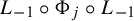 $L_{-1}\circ \Phi _j\circ L_{-1}$
is a Fatou coordinate of
$L_{-1}\circ \Phi _j\circ L_{-1}$
is a Fatou coordinate of
 $\widetilde g^{-1}$
on
$\widetilde g^{-1}$
on
 $\widetilde S_{j+1}$
. Indeed, we have
$\widetilde S_{j+1}$
. Indeed, we have
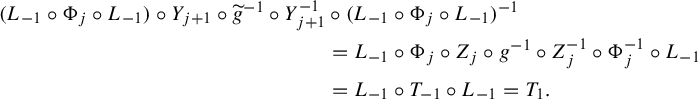 $$ \begin{align*} (L_{-1}\circ \Phi_j\circ L_{-1})\circ Y_{j+1} \circ \widetilde g^{-1}\circ Y_{j+1}^{-1} & {}\circ (L_{-1}\circ \Phi_j\circ L_{-1})^{-1}\\ &= L_{-1}\circ \Phi_j\circ Z_j\circ g^{-1}\circ Z_j^{-1}\circ \Phi_j^{-1}\circ L_{-1}\\ &= L_{-1} \circ T_{-1}\circ L_{-1} = T_1. \end{align*} $$
It follows that the transition functions
 $\widetilde \Psi _j$
of
$\widetilde \Psi _j$
of
 $\widetilde g^{-1}$
are given by, for
$\widetilde g^{-1}$
are given by, for
 $j{\kern-1pt}\not =1,k$
odd,
$j{\kern-1pt}\not =1,k$
odd,
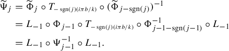 $$ \begin{align*} \widetilde \Psi_j &= \widetilde \Phi_j\circ T_{\scriptscriptstyle-\mathop{\mathrm{sgn}}\nolimits(j){(i\pi b/ k)}} \circ (\widetilde \Phi_{j - \mathop{\mathrm{sgn}}\nolimits(j)})^{-1}\\ &= L_{-1}\circ \Phi_{j-1} \circ T_{\scriptscriptstyle-\mathop{\mathrm{sgn}}\nolimits(j){(i\pi b/ k)}} \circ \Phi_{j-1-\mathop{\mathrm{sgn}}\nolimits(j-1)}^{-1} \circ L_{-1}\\ &= L_{-1} \circ \Psi_{j-1}^{-1}\circ L_{-1}. \end{align*} $$
The other values of j are done similarly. Note however that for
 $j=1$
, the equation becomes
$j=1$
, the equation becomes
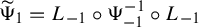 $\widetilde \Psi _1 = L_{-1}\circ \Psi _{-1}^{-1}\circ L_{-1}$
and that, for
$\widetilde \Psi _1 = L_{-1}\circ \Psi _{-1}^{-1}\circ L_{-1}$
and that, for
 $j=k$
, we have
$j=k$
, we have
 $\widetilde \Psi _{-k} = L_{-1}\circ \Psi _k^{-1}\circ L_{-1}$
.
$\widetilde \Psi _{-k} = L_{-1}\circ \Psi _k^{-1}\circ L_{-1}$
.
6 Space of orbits and classification under analytic conjugacy
When two antiholomorphic parabolic germs are analytically conjugate, it is clear that their spaces of orbits are essentially the same. Our guiding principle is that the space of orbits completely describes the dynamics of the germs; when two germs have the same space of orbits, they should be analytically conjugate. A formal statement will be given in the form of the classification theorem (Theorem 6.3) in §6.3.
6.1 Description of the space of orbits
The space of orbits in the holomorphic case is well known. It is briefly described in [Reference Ilyashenko5]. We will introduce the objects from the holomorphic case needed for the antiholomorphic description.
In each Fatou coordinate of f (and
 $f \circ f$
), we may choose a fundamental domain of
$f \circ f$
), we may choose a fundamental domain of
 $g = f\circ f$
by taking any vertical strip
$g = f\circ f$
by taking any vertical strip
 $B_j$
of width one. We quotient by the action of
$B_j$
of width one. We quotient by the action of
 $T_1$
, obtaining the bi-infinite Écalle cylinders. Some orbits of g will appear in two consecutive cylinders. Since
$T_1$
, obtaining the bi-infinite Écalle cylinders. Some orbits of g will appear in two consecutive cylinders. Since
 $\Psi _j \circ T_1 = T_1\circ \Psi _j$
, we identify together those orbits by identifying
$\Psi _j \circ T_1 = T_1\circ \Psi _j$
, we identify together those orbits by identifying
 $W_j$
with
$W_j$
with
 $\Psi _j(W_j)$
(or
$\Psi _j(W_j)$
(or
 $\Psi _j^{-1}(W_j)$
depending on j).
$\Psi _j^{-1}(W_j)$
depending on j).
The universal covering
 $E\colon \mathbb {C}\to \mathbb {C}^\ast $
given by
$E\colon \mathbb {C}\to \mathbb {C}^\ast $
given by
 $w = E(W) = \exp (-2i\pi W)$
is a biholomorphism of each cylinder onto
$w = E(W) = \exp (-2i\pi W)$
is a biholomorphism of each cylinder onto
 $\mathbb {C}^\ast $
. This allows us to see the Écalle cylinders as Riemann spheres punctured at
$\mathbb {C}^\ast $
. This allows us to see the Écalle cylinders as Riemann spheres punctured at
 $0$
and infinity
$0$
and infinity
 $\mathbb S^2_j\setminus \{0,\infty \}$
(see Figure 15). We will define the horn maps using this universal covering.
$\mathbb S^2_j\setminus \{0,\infty \}$
(see Figure 15). We will define the horn maps using this universal covering.
A fundamental domain obtained by
 $Z_0^{-1}(B_0)$
in the z-coordinate (in grey) and the sphere it represents.
$Z_0^{-1}(B_0)$
in the z-coordinate (in grey) and the sphere it represents.
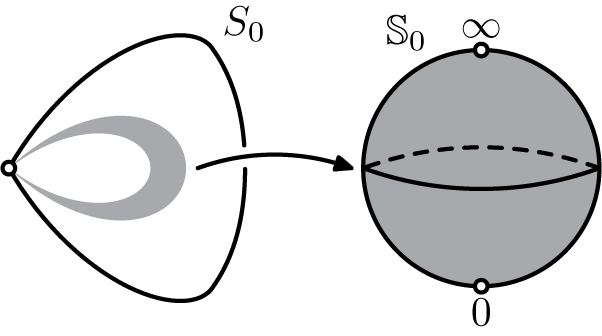
Definition 6.1. The horn maps
 $\psi _j$
, for
$\psi _j$
, for
 $j=1,\ldots ,k$
, are defined by
$j=1,\ldots ,k$
, are defined by
 $\psi _j = E\circ \Psi _j\circ E^{-1}$
, where
$\psi _j = E\circ \Psi _j\circ E^{-1}$
, where
 $\Psi _j$
is a transition function and
$\Psi _j$
is a transition function and
 $$ \begin{align} E(W) = \exp(-2i\pi W). \end{align} $$
For positive j odd (respectively j even), the horn maps are defined on a punctured neighbourhood of the origin (respectively of infinity) with their image in a neighbourhood punctured of the origin (respectively of infinity). By the Riemann removable singularity theorem, they extend to
 $$ \begin{align*}\psi_j \colon \begin{cases} (\mathbb{C},0) \to (\mathbb{C},0) & \textrm{for }j> 0\textrm{ odd,}\\ (\mathbb{C},\infty) \to (\mathbb{C},\infty) & \textrm{for }j > 0\textrm{ even.} \end{cases} \end{align*} $$
To retrieve the
 $\psi _j$
for
$\psi _j$
for
 $j < 0$
, we use equation (17) in the coordinate
$j < 0$
, we use equation (17) in the coordinate
 $w = E(W)$
 $$ \begin{align} \psi_{-j} = L_{-1}\circ \tau \circ \psi_j \circ L_{-1}\circ \tau, \end{align} $$
where
 $L_{-1}(w) = -w$
and
$L_{-1}(w) = -w$
and
 $\tau (w) = {1 / {\overline w}}$
.
$\tau (w) = {1 / {\overline w}}$
.
The space of orbits of
 $g = f\circ f$
is described by the
$g = f\circ f$
is described by the
 $2k$
spheres with identifications at the origin or at infinity, as seen in Figure 16.
$2k$
spheres with identifications at the origin or at infinity, as seen in Figure 16.
Space of orbits for
 $f\circ f$
of codimension four.
$f\circ f$
of codimension four.
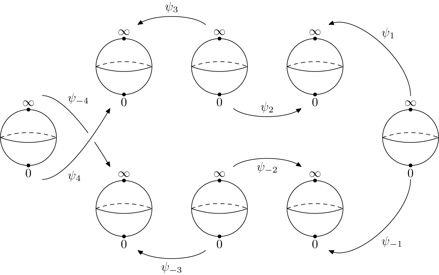
Remark 6.2. By differentiating
 $E\circ \Psi _j \circ E^{-1}$
, we obtain
$E\circ \Psi _j \circ E^{-1}$
, we obtain
 $$ \begin{align} \begin{aligned} {(\psi_j)}'(\infty) &= e^{{2\pi^2b/ k}}\quad\textrm{for }j\textrm{ odd,}\\ {(\psi_j)}'(0) &= e^{{2\pi^2b/ k}}\quad\textrm{for }j\textrm{ even,} \end{aligned} \end{align} $$
so the product of those derivatives for
 $j\in \{-k,\ldots ,-1\}\cup \{1,\ldots ,k\}$
is
$j\in \{-k,\ldots ,-1\}\cup \{1,\ldots ,k\}$
is
 $e^{4\pi ^2 b}$
.
$e^{4\pi ^2 b}$
.
6.2 The space of orbits of f
The complex conjugation
 $\Sigma $
becomes
$\Sigma $
becomes
 $\tau (w) = {1/\overline w}$
on the spheres, where
$\tau (w) = {1/\overline w}$
on the spheres, where
 $w\in \mathbb S_j^2$
and
$w\in \mathbb S_j^2$
and
 $\tau (w)\in \mathbb S_{-j}^2$
. The translation
$\tau (w)\in \mathbb S_{-j}^2$
. The translation
 ${T_{\scriptscriptstyle {1/2}}}$
becomes
${T_{\scriptscriptstyle {1/2}}}$
becomes
 $L_{-1}(w) = -w$
. In the Fatou coordinates, f is
$L_{-1}(w) = -w$
. In the Fatou coordinates, f is
 $\Sigma \circ {T_{\scriptscriptstyle {1/2}}}$
, so that on the spheres, f is
$\Sigma \circ {T_{\scriptscriptstyle {1/2}}}$
, so that on the spheres, f is
 $L_{-1}\circ \tau (w) = -{1/\overline w}$
. To obtain the space of orbits of f, we identify w and
$L_{-1}\circ \tau (w) = -{1/\overline w}$
. To obtain the space of orbits of f, we identify w and
 $L_{-1}\circ \tau (w)$
in the space of orbits of
$L_{-1}\circ \tau (w)$
in the space of orbits of
 $f \circ f$
, that is, on the
$f \circ f$
, that is, on the
 $2k$
spheres above.
$2k$
spheres above.
Let us first consider the case of codimension one, so that we have two sectors
 $S_0$
and
$S_0$
and
 $S_1=S_{-1}$
in the z-coordinate and two spheres
$S_1=S_{-1}$
in the z-coordinate and two spheres
 $\mathbb S_0^2$
and
$\mathbb S_0^2$
and
 $\mathbb S_1^2$
. Recall that for
$\mathbb S_1^2$
. Recall that for
 $z\in S_0$
,
$z\in S_0$
,
 $f^{-1}(z)$
is still in
$f^{-1}(z)$
is still in
 $S_0$
. This means that
$S_0$
. This means that
 $L_{-1}\circ \tau $
acts on
$L_{-1}\circ \tau $
acts on
 $\mathbb S_0^2$
. It sends
$\mathbb S_0^2$
. It sends
 $0$
to
$0$
to
 $\infty $
, the northern hemisphere to the southern hemisphere, and the equator on itself. On the equator
$\infty $
, the northern hemisphere to the southern hemisphere, and the equator on itself. On the equator
 $|w|=1$
, we identify w to
$|w|=1$
, we identify w to
 $-w$
. The resulting surface is the real projective space
$-w$
. The resulting surface is the real projective space
 $\mathbb {R}\mathbb P^2$
. This is also true for
$\mathbb {R}\mathbb P^2$
. This is also true for
 $S_1$
and
$S_1$
and
 $\mathbb S_1^2$
. The equators of both spheres play a special role; they each represent orbits along an invariant half-curve that each forms a ‘semi-axis’ of reflection for f.
$\mathbb S_1^2$
. The equators of both spheres play a special role; they each represent orbits along an invariant half-curve that each forms a ‘semi-axis’ of reflection for f.
Therefore, in codimension one, the space of orbits is two real projective spaces with one germ of a holomorphic diffeomorphism
 $$ \begin{align*}[\psi_1]\colon (\mathbb{R}\mathbb P^2,[0])\to (\mathbb{R}\mathbb P^2,[0]),\end{align*} $$
where
 $[\psi _1]$
is the equivalence class of
$[\psi _1]$
is the equivalence class of
 $\psi _1$
under the quotient of
$\psi _1$
under the quotient of
 $\mathbb S^2$
to
$\mathbb S^2$
to
 $\mathbb {R}\mathbb P^2$
and
$\mathbb {R}\mathbb P^2$
and
 $[0]$
is the equivalence class of the points
$[0]$
is the equivalence class of the points
 $\{0,\infty \}$
identified together. The class
$\{0,\infty \}$
identified together. The class
 $[\psi _1]$
is well defined, since
$[\psi _1]$
is well defined, since
 $\psi _1\circ L_{-1}\circ \tau = \tau \circ L_{-1}\circ \psi _{-1}$
.
$\psi _1\circ L_{-1}\circ \tau = \tau \circ L_{-1}\circ \psi _{-1}$
.
In codimension
 $k>1$
, the spheres
$k>1$
, the spheres
 $\mathbb S_0$
and
$\mathbb S_0$
and
 $\mathbb S_k$
both quotient to a real projective space, but the other spheres are identified in pairs
$\mathbb S_k$
both quotient to a real projective space, but the other spheres are identified in pairs
 $(\mathbb S_j,\mathbb S_{-j})$
, so that the quotient of the union of the two spheres is diffeomorphic to a sphere. The space of orbits is then described by two real projective spaces together with
$(\mathbb S_j,\mathbb S_{-j})$
, so that the quotient of the union of the two spheres is diffeomorphic to a sphere. The space of orbits is then described by two real projective spaces together with
 $k-1$
spheres and k equivalence classes of horn maps
$k-1$
spheres and k equivalence classes of horn maps
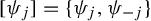 $[\psi _j] = \{\psi _j,\psi _{-j}\}$
. The class
$[\psi _j] = \{\psi _j,\psi _{-j}\}$
. The class
 $[\psi _j]$
defines a germ at
$[\psi _j]$
defines a germ at
 $[0]=[\infty ]$
on the quotiented spheres
$[0]=[\infty ]$
on the quotiented spheres
 $(\mathbb S_j,\mathbb S_{-j})$
, since the representatives satisfy
$(\mathbb S_j,\mathbb S_{-j})$
, since the representatives satisfy
 $\psi _j\circ L_{-1}\circ \tau = L_{-1}\circ \tau \circ \psi _{-j}$
.
$\psi _j\circ L_{-1}\circ \tau = L_{-1}\circ \tau \circ \psi _{-j}$
.
On the two extreme projective spaces we have a distinguished curve given by the equator. The only changes of coordinates on
 $\mathbb D$
preserving the equator and sending opposite points to opposite points are the linear maps
$\mathbb D$
preserving the equator and sending opposite points to opposite points are the linear maps
 $L_c$
with
$L_c$
with
 $|c|=1$
. Hence, the lines
$|c|=1$
. Hence, the lines
 $\textrm{Im}\kern2pt W = y$
are invariant. This y is the generalization of the Écalle height introduced in [Reference Hubbard and Schleicher4]. However, on the other spheres, there does not appear to be a quantity preserved by changes of coordinates.
$\textrm{Im}\kern2pt W = y$
are invariant. This y is the generalization of the Écalle height introduced in [Reference Hubbard and Schleicher4]. However, on the other spheres, there does not appear to be a quantity preserved by changes of coordinates.
The space of orbits of f in codimension four.
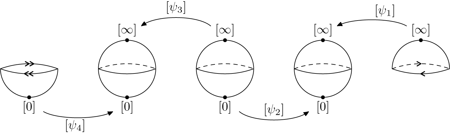
The two projective spaces correspond to the orbits of two Fatou petals containing the formal symmetry axis of f. The equator of each projective space corresponds to a semi-axis of symmetry in each respective petal. These axes meet at the origin, but generally they cannot be extended into a real analytic curve. We will see in Theorem 7.6 exactly when they extend into a real analytic curve. This formal symmetry axis explains the existence of the Écalle height in the two projective spaces and why the Écalle height does not exist in the other spheres.
6.3 Classification under analytic conjugacy
We can now state and prove the main theorem of this paper.
Classification Theorem 6.3. For antiholomorphic parabolic germs of codimension k (and of positive type when k is even), we have:
-
(1) the modulus of classification is a complete invariant of analytic classification under holomorphic conjugacy;
-
(2) the moduli space is the set of
$(k,b,[\Psi _1,\ldots ,\Psi _k])$
, where the constant terms of
$\Psi _j$
satisfy (20), and
$[\Psi _1,\ldots ,\Psi _k]$
is the equivalence class under the relation (21) (and (22) for k even).

Proof The proof is analogous to that in the holomorphic case, which can be found in [Reference Ilyashenko5, Reference Ilyashenko and Yakovenko6].
(1) Let
 $f_\ell \colon (\mathbb {C},0) \to (\mathbb {C},0)$
be a germ of an antiholomorphic diffeomorphism with a parabolic fixed point at the origin and let
$f_\ell \colon (\mathbb {C},0) \to (\mathbb {C},0)$
be a germ of an antiholomorphic diffeomorphism with a parabolic fixed point at the origin and let
 $(k_\ell ,b_\ell ,[\Psi _{1,\ell },\ldots ,\Psi _{k,\ell }])$
be its modulus of classification for
$(k_\ell ,b_\ell ,[\Psi _{1,\ell },\ldots ,\Psi _{k,\ell }])$
be its modulus of classification for
 $\ell =1,2$
. We can of course suppose that
$\ell =1,2$
. We can of course suppose that
 $f_\ell $
is prenormalized.
$f_\ell $
is prenormalized.
Suppose first that
 $f_2(u) = h\circ f_1\circ h^{-1}(u)$
for some germ of an analytic diffeomorphism
$f_2(u) = h\circ f_1\circ h^{-1}(u)$
for some germ of an analytic diffeomorphism
 $u = h(z)$
. The germs
$u = h(z)$
. The germs
 $f_1$
and
$f_1$
and
 $f_2$
must have the same codimension and formal invariant, since they are topological and formal invariants. For the analytic invariant, first let
$f_2$
must have the same codimension and formal invariant, since they are topological and formal invariants. For the analytic invariant, first let
 $F_1$
,
$F_1$
,
 $F_2$
and H denote the expressions of
$F_2$
and H denote the expressions of
 $f_1$
,
$f_1$
,
 $f_2$
, and h in the time coordinate. If
$f_2$
, and h in the time coordinate. If
 $\Phi _j$
is a Fatou coordinate of
$\Phi _j$
is a Fatou coordinate of
 $F_2$
on
$F_2$
on
 $U_j$
, then
$U_j$
, then
 $\Phi _j\circ H$
is a Fatou coordinate of
$\Phi _j\circ H$
is a Fatou coordinate of
 $F_1$
. It follows that they have the same transition functions.
$F_1$
. It follows that they have the same transition functions.
Conversely, suppose that
 $f_1$
and
$f_1$
and
 $f_2$
have the same modulus. We can choose a common normalized representative
$f_2$
have the same modulus. We can choose a common normalized representative
 $(\Psi _1,\ldots ,\Psi _k)$
for both classes and Fatou coordinates
$(\Psi _1,\ldots ,\Psi _k)$
for both classes and Fatou coordinates
 $\Phi _{j,\ell }$
for
$\Phi _{j,\ell }$
for
 $f_\ell $
(
$f_\ell $
(
 $\ell =1,2$
) such that the
$\ell =1,2$
) such that the
 $\Psi _j$
are the transition maps for these Fatou coordinates. Let
$\Psi _j$
are the transition maps for these Fatou coordinates. Let
 $\varphi _{j,\ell } = Z_j^{-1}\circ \Phi _{j,\ell }\circ Z_j$
, for
$\varphi _{j,\ell } = Z_j^{-1}\circ \Phi _{j,\ell }\circ Z_j$
, for
 $\ell =1,2$
, be the expression of Fatou coordinates in the z-coordinate. Then we define
$\ell =1,2$
, be the expression of Fatou coordinates in the z-coordinate. Then we define
 $$ \begin{align*}h_j(z) = \varphi_{j,1}^{-1}\circ \varphi_{j,2}(z) \end{align*} $$
on
 $S_j$
. It sends the orbits of
$S_j$
. It sends the orbits of
 $f_2$
to those of
$f_2$
to those of
 $f_1$
on
$f_1$
on
 $S_j$
. On the intersection of two consecutive sectors
$S_j$
. On the intersection of two consecutive sectors
 $S_j\cap S_{j+1}$
, we see that
$S_j\cap S_{j+1}$
, we see that
 $$ \begin{align*}h_{j+1}\circ h_j^{-1}(z) = \mathrm{id}, \end{align*} $$
so the
 $h_j$
agree on the intersection. We may define h on
$h_j$
agree on the intersection. We may define h on
 $\bigcup _j S_j$
by
$\bigcup _j S_j$
by
 $h(z) = h_j(z)$
if
$h(z) = h_j(z)$
if
 $z\in S_j$
. It sends a punctured neighbourhood of the origin into another punctured neighbourhood of the origin, so, by the Riemann removable singularity theorem, h extends to a holomorphic diffeomorphism of a neighbourhood of the origin.
$z\in S_j$
. It sends a punctured neighbourhood of the origin into another punctured neighbourhood of the origin, so, by the Riemann removable singularity theorem, h extends to a holomorphic diffeomorphism of a neighbourhood of the origin.
Finally, we see that
 $h\circ f_2 = f_1 \circ h$
, since it sends the orbits of
$h\circ f_2 = f_1 \circ h$
, since it sends the orbits of
 $f_2$
to the orbits of
$f_2$
to the orbits of
 $f_1$
on a whole neighbourhood of the origin.
$f_1$
on a whole neighbourhood of the origin.
(2) The proof is in two steps. First we construct an abstract Riemann surface S on which
 $\Sigma \circ {T_{\scriptscriptstyle {1/2}}}$
is well defined and we prove that this surface has the conformal type of a punctured disk. Then we prove that
$\Sigma \circ {T_{\scriptscriptstyle {1/2}}}$
is well defined and we prove that this surface has the conformal type of a punctured disk. Then we prove that
 $\Sigma \circ {T_{\scriptscriptstyle {1/2}}}$
is the germ we are looking for on the disk.
$\Sigma \circ {T_{\scriptscriptstyle {1/2}}}$
is the germ we are looking for on the disk.
Consider a triple
 $(k,b, [\Psi _1,\ldots ,\Psi _k])$
. We must find a parabolic germ of an antiholomorphic diffeomorphism with this modulus of classification.
$(k,b, [\Psi _1,\ldots ,\Psi _k])$
. We must find a parabolic germ of an antiholomorphic diffeomorphism with this modulus of classification.
Let
 $(\Psi _1,\ldots ,\Psi _k)$
be a representative of the analytic invariant and let
$(\Psi _1,\ldots ,\Psi _k)$
be a representative of the analytic invariant and let
 $\Psi _{-1},\ldots ,\Psi _{-k}$
be the other transition functions obtained from (17). Let
$\Psi _{-1},\ldots ,\Psi _{-k}$
be the other transition functions obtained from (17). Let
 $\sigma \circ v^{\scriptscriptstyle {1/2}}$
be the normal form of codimension k with formal invariant b. Let
$\sigma \circ v^{\scriptscriptstyle {1/2}}$
be the normal form of codimension k with formal invariant b. Let
 $U_j$
be the charts in the time coordinate of v.
$U_j$
be the charts in the time coordinate of v.
We consider the transition functions defined on those charts. More precisely,
 $\Psi _1$
is defined on a domain of
$\Psi _1$
is defined on a domain of
 $U_0$
containing an upper half-plane with its image in
$U_0$
containing an upper half-plane with its image in
 $U_1$
;
$U_1$
;
 $\Psi _2$
is defined on a domain of
$\Psi _2$
is defined on a domain of
 $U_2$
containing a lower half-plane with its image in
$U_2$
containing a lower half-plane with its image in
 $U_1$
, and so on. We define the Riemann surface S by
$U_1$
, and so on. We define the Riemann surface S by
 $$ \begin{align*}S = \bigsqcup_{j=-k}^k U_j/\sim, \end{align*} $$
where
 $\sim $
identifies
$\sim $
identifies
 $W_j\in U_j$
with its image by
$W_j\in U_j$
with its image by
 $\Psi _j$
or
$\Psi _j$
or
 $\Psi _{j-1}$
(depending on j). As is done in [Reference Ilyashenko and Yakovenko6], we can build a smooth quasi-conformal mapping
$\Psi _{j-1}$
(depending on j). As is done in [Reference Ilyashenko and Yakovenko6], we can build a smooth quasi-conformal mapping
 $P\colon S\to \mathbb {C}^\ast $
and, from the Ahlfors–Bers theorem (see [Reference Ahlfors1]), find a diffeomorphism
$P\colon S\to \mathbb {C}^\ast $
and, from the Ahlfors–Bers theorem (see [Reference Ahlfors1]), find a diffeomorphism
 $Q\colon D \to (\mathbb {C},0)$
, where
$Q\colon D \to (\mathbb {C},0)$
, where
 $D = P(S)\cup \{0\}$
, so that the composition
$D = P(S)\cup \{0\}$
, so that the composition
 $H = Q\circ P\colon S\to (\mathbb {C},0)$
is holomorphic. In fact, H is a biholomorphism of S onto some punctured disk of the origin.
$H = Q\circ P\colon S\to (\mathbb {C},0)$
is holomorphic. In fact, H is a biholomorphism of S onto some punctured disk of the origin.
By (15), we know that
 $\Sigma \circ {T_{\scriptscriptstyle {1/2}}}$
is well defined on S. The map
$\Sigma \circ {T_{\scriptscriptstyle {1/2}}}$
is well defined on S. The map
 $f = H\circ \Sigma \circ {T_{\scriptscriptstyle {1/2}}}\circ H^{-1}$
extends to the origin by
$f = H\circ \Sigma \circ {T_{\scriptscriptstyle {1/2}}}\circ H^{-1}$
extends to the origin by
 $f(0) = 0$
, since it is bounded around
$f(0) = 0$
, since it is bounded around
 $0$
(we can apply the Riemann removable singularity theorem to
$0$
(we can apply the Riemann removable singularity theorem to
 $f\circ \sigma $
to see this). Lastly,
$f\circ \sigma $
to see this). Lastly,
 $T_1$
is also well defined on S, so we set
$T_1$
is also well defined on S, so we set
 $g = H\circ T_1\circ H^{-1}$
. Since
$g = H\circ T_1\circ H^{-1}$
. Since
 $T_1 = (\Sigma \circ {T_{\scriptscriptstyle {1/2}}})\circ (\Sigma \circ {T_{\scriptscriptstyle {1/2}}})$
, it follows that
$T_1 = (\Sigma \circ {T_{\scriptscriptstyle {1/2}}})\circ (\Sigma \circ {T_{\scriptscriptstyle {1/2}}})$
, it follows that
 $g = f\circ f$
and, by the chain rule,
$g = f\circ f$
and, by the chain rule,
 $|{\partial f/ \partial {\overline z}}|^2 = g'(0)$
. By the holomorphic case, we know that g is a holomorphic parabolic germ of codimension k, so it follows that f is parabolic and of codimension k. The formal invariant of f is b, since it is determined by (19).
$|{\partial f/ \partial {\overline z}}|^2 = g'(0)$
. By the holomorphic case, we know that g is a holomorphic parabolic germ of codimension k, so it follows that f is parabolic and of codimension k. The formal invariant of f is b, since it is determined by (19).
It remains only to prove that f is of positive type. The formal symmetry axis of f is the real line, since the
 $\Psi _1$
and
$\Psi _1$
and
 $\Psi _{-1}$
are defined on
$\Psi _{-1}$
are defined on
 $U_0$
and
$U_0$
and
 $\Psi _j\circ \Sigma \circ {T_{\scriptscriptstyle {1/2}}} = \Sigma \circ {T_{\scriptscriptstyle {1/2}}}\circ \Psi _{-j}$
. Moreover, the petal
$\Psi _j\circ \Sigma \circ {T_{\scriptscriptstyle {1/2}}} = \Sigma \circ {T_{\scriptscriptstyle {1/2}}}\circ \Psi _{-j}$
. Moreover, the petal
 $S_0$
of f is repulsive, since
$S_0$
of f is repulsive, since
 $H\big |_{U_0}\circ Z_0\colon U_0\to U_0$
is a Fatou coordinate of f and
$H\big |_{U_0}\circ Z_0\colon U_0\to U_0$
is a Fatou coordinate of f and
 $U_0$
contains a half-plane
$U_0$
contains a half-plane
 $\{\Re Z < R\}$
, that is,
$\{\Re Z < R\}$
, that is,
 $S_0$
contains all the backward iterates of f. Therefore, f is of positive type.
$S_0$
contains all the backward iterates of f. Therefore, f is of positive type.
We conclude that f is a germ with modulus
 $(k,b,[\Psi _1,\ldots ,\Psi _k])$
.
$(k,b,[\Psi _1,\ldots ,\Psi _k])$
.
7 Applications of the classification theorem
Here, we will solve Questions 1 to 5 of the introduction and other related questions.
Questions 1, 3, and 5 have holomorphic counterparts that are respectively about the extraction of holomorphic roots, the embedding in a flow, and the centralizer of a holomorphic parabolic germ. The answer to these questions can be found in [Reference Ilyashenko and Yakovenko6] or in [Reference Loray8, §2.8].
7.1 Embedding in a flow or the complex conjugate of a flow
If a holomorphic germ g is conjugate to the normal form, that is,
 $g = h\circ v^{\scriptscriptstyle 1}\circ h^{-1}$
, then it is embedded in the family
$g = h\circ v^{\scriptscriptstyle 1}\circ h^{-1}$
, then it is embedded in the family
 $g_t = h\circ v^t\circ h^{-1}$
. Similarly, we will say that f is embeddable if it is embedded in the family
$g_t = h\circ v^t\circ h^{-1}$
. Similarly, we will say that f is embeddable if it is embedded in the family
 $f_t:=h\circ \sigma \circ v^t\circ h^{-1}$
. When is an antiholomorphic parabolic germ embeddable? This corresponds to Question 3. The answer is read in the modulus of classification.
$f_t:=h\circ \sigma \circ v^t\circ h^{-1}$
. When is an antiholomorphic parabolic germ embeddable? This corresponds to Question 3. The answer is read in the modulus of classification.
Theorem 7.1. (Embedding in a flow)
An antiholomorphic parabolic germ f is analytically conjugate to its normal form (that is, embeddable) if and only if the transition functions of f are translations.
Proof The transition functions of the normal form are translations, since the time charts
 $Z_j$
are Fatou coordinates. Therefore, it follows from the classification theorem (Theorem 6.3).
$Z_j$
are Fatou coordinates. Therefore, it follows from the classification theorem (Theorem 6.3).
In Proposition 2.3, we proved that f is always formally conjugate to the sum of a formal germ with real coefficients. We ask the related question.
Questions 7.2. When is a parabolic antiholomorphic germ analytically conjugate to a germ with real coefficients?
Of course, this is the case for any embeddable germ. But we will show in §7.3 that the embeddable germs form a subset of infinite codimension in the set of antiholomorphic parabolic germs conjugate to a germ with real coefficients. We first tackle Question 1.
7.2 Antiholomorphic
$\boldsymbol {n}$
th root problem

Question 1 and its restatement Question 3.5, as well as Question 3.6, are concerned with the existence of antiholomorphic roots and their uniqueness.
Theorem 7.3. (Antiholomorphic root extraction problem)
Let g be a holomorphic parabolic germ and let
 $(k,b,[\Psi _{-k},\ldots ,\Psi _{-1},\Psi _1,\ldots ,\Psi _k])$
be its Écalle–Voronin modulus (see §5.1), then:
$(k,b,[\Psi _{-k},\ldots ,\Psi _{-1},\Psi _1,\ldots ,\Psi _k])$
be its Écalle–Voronin modulus (see §5.1), then:
-
(1) g has k one-parameter families of formal antiholomorphic nth roots, one for each of the k formal axes of reflection;
-
(2) g has an antiholomorphic nth root (n even) tangent to the formal symmetry axis
$e^{i \pi \ell /k}\mathbb {R}$
if and only if there exists a representative
$(\Psi _{-k},\ldots ,\Psi _{-1}$
,
$\Psi _1,\ldots ,\Psi _k)$
of the equivalence relation (23) which has a symmetry property with respect to the formal symmetry axis
$e^{i\pi \ell /k}\mathbb {R}$
, namely (33)where
$$ \begin{align} \Psi_j \circ \Sigma\circ T_{{1/n}} = \Sigma \circ T_{{1/n}} \circ \Psi_{s_\ell(j)}, \end{align} $$
$s_\ell $
is the reflection of indices with respect to
$e^{i\pi \ell /k}\mathbb {R}$
(see Definition 5.5);
-
(3) if g is not analytically conjugate to its normal form, then:
-
(i) each family has at most one convergent root, so g has at most k distinct antiholomorphic nth roots
$f_j$
; -
(ii) if g has m distinct antiholomorphic roots
$f_{\ell _1}$
,
$\ldots $
,
$f_{\ell _m}$
with distinct linear parts
$e^{2i\pi \ell _j/k}{\overline z}$
,
$j=1,\ldots ,m$
, then the modulus of g has
$\gcd (\ell _m-\ell _1,\ldots ,\ell _m-\ell _{m-1},k)$
independent transition functions.
-

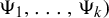


Proof (1) That g has a one-parameter family of formal antiholomorphic nth roots on each symmetry axis is a consequence of the fact that g is formally conjugate to the normal form
 $v^{\scriptscriptstyle 1}$
and Proposition 3.4.
$v^{\scriptscriptstyle 1}$
and Proposition 3.4.
(2) We first prove this for the case k odd. Let
 $$ \begin{align*}\boldsymbol{\Psi} = (\Psi_{-k},\ldots,\Psi_{-1},\Psi_1,\ldots,\Psi_k) \end{align*} $$
be a representative of the analytic invariant of g.
First, we suppose that the representative satisfies (33). To realize an antiholomorphic root tangent to the symmetry axis
 $e^{2i\pi \ell / k}\mathbb {R}$
, we rotate the coordinate by
$e^{2i\pi \ell / k}\mathbb {R}$
, we rotate the coordinate by
 $R_\ell (z) = e^{-{2i\pi \ell /k}}z$
so that this axis is on the real line and the dynamics of
$R_\ell (z) = e^{-{2i\pi \ell /k}}z$
so that this axis is on the real line and the dynamics of
 $R_\ell \circ g\circ R_\ell ^{-1}$
on the side of the positive real axis is repulsive. Let
$R_\ell \circ g\circ R_\ell ^{-1}$
on the side of the positive real axis is repulsive. Let
 $g_\ell = R_\ell \circ g\circ R_\ell ^{-1}$
and let r correspond to the permutation of indices defined by
$g_\ell = R_\ell \circ g\circ R_\ell ^{-1}$
and let r correspond to the permutation of indices defined by
 $R_\ell $
(see Definition 5.5). The representative is permuted into
$R_\ell $
(see Definition 5.5). The representative is permuted into
 $(\Psi _{r(-k)},\ldots ,\Psi _{r(-1)},\Psi _{r(1)},\ldots ,\Psi _{r(k)})$
. Also, we have that
$(\Psi _{r(-k)},\ldots ,\Psi _{r(-1)},\Psi _{r(1)},\ldots ,\Psi _{r(k)})$
. Also, we have that
 $r^{-1} s_\ell r = s_0$
, where
$r^{-1} s_\ell r = s_0$
, where
 $s_0(j) = -j$
and
$s_0(j) = -j$
and
 $s_\ell $
is the reflection of indices induced by
$s_\ell $
is the reflection of indices induced by
 $\sigma _\ell $
. Equation (33) becomes
$\sigma _\ell $
. Equation (33) becomes
 $$ \begin{align*}\Psi_{r(j)}\circ \Sigma\circ{T_{\scriptscriptstyle{1/2}}} = \Sigma\circ{T_{\scriptscriptstyle{1/2}}} \circ \Psi_{r(-j)}. \end{align*} $$
Now we may repeat the proof of part (2) of Theorem 6.3 to obtain an antiholomorphic germ
 $f_\ell \colon (\mathbb {C},0)\to (\mathbb {C},0)$
with analytic invariant
$f_\ell \colon (\mathbb {C},0)\to (\mathbb {C},0)$
with analytic invariant
 $[\Psi _{r(1)},\ldots ,\Psi _{r(k)}]$
such that
$[\Psi _{r(1)},\ldots ,\Psi _{r(k)}]$
such that
 $f_\ell $
is
$f_\ell $
is
 $\Sigma \circ T_{{1/n}}$
in each Fatou coordinate of
$\Sigma \circ T_{{1/n}}$
in each Fatou coordinate of
 $g_\ell $
. Since
$g_\ell $
. Since
 $(\Sigma \circ T_{{1/n}})^{\circ n} = T_1$
in the Fatou coordinates, it follows that
$(\Sigma \circ T_{{1/n}})^{\circ n} = T_1$
in the Fatou coordinates, it follows that
 $f_\ell ^{\circ n} = g_\ell $
.
$f_\ell ^{\circ n} = g_\ell $
.
Conversely, suppose that g has an nth root
 $f_\ell $
tangent to the reflection axis
$f_\ell $
tangent to the reflection axis
 $e^{2i\pi \ell /k}\mathbb {R}$
. We rotate the coordinate by
$e^{2i\pi \ell /k}\mathbb {R}$
. We rotate the coordinate by
 $R_\ell $
. Let
$R_\ell $
. Let
 $f = R_\ell \circ f_\ell \circ R_\ell ^{-1}$
. Now, in every Fatou coordinate of
$f = R_\ell \circ f_\ell \circ R_\ell ^{-1}$
. Now, in every Fatou coordinate of
 $g_\ell $
, f has the form
$g_\ell $
, f has the form
 $\Sigma \circ T_{(1/n)+iy}$
, by Proposition 3.4. By changing Fatou coordinates, we may obtain
$\Sigma \circ T_{(1/n)+iy}$
, by Proposition 3.4. By changing Fatou coordinates, we may obtain
 $\Sigma \circ T_{{1/ n}}$
. Those Fatou coordinates give us a representative
$\Sigma \circ T_{{1/ n}}$
. Those Fatou coordinates give us a representative
 $(\Psi _{-k}',\ldots ,\Psi _{-1}',\Psi _1',\ldots , \Psi _k')$
that is equivalent to
$(\Psi _{-k}',\ldots ,\Psi _{-1}',\Psi _1',\ldots , \Psi _k')$
that is equivalent to
 $\boldsymbol {\Psi }$
under the relations (23) and (24) and that satisfies
$\boldsymbol {\Psi }$
under the relations (23) and (24) and that satisfies
 $$ \begin{align*}\Psi_{j}'\circ \Sigma\circ{T_{\scriptscriptstyle{1/2}}} = \Sigma\circ{T_{\scriptscriptstyle{1/2}}} \circ \Psi_{-j}'. \end{align*} $$
It follows that
 $(\Psi _{r^{-1}(-k)}',\ldots ,\Psi _{r^{-1}(-1)}',\Psi _{r^{-1}(1)}',\ldots ,\Psi _{r^{-1}(k)}')$
is a representative equivalent to
$(\Psi _{r^{-1}(-k)}',\ldots ,\Psi _{r^{-1}(-1)}',\Psi _{r^{-1}(1)}',\ldots ,\Psi _{r^{-1}(k)}')$
is a representative equivalent to
 $\boldsymbol {\Psi }$
under relation (23) which satisfies (33), using the fact that
$\boldsymbol {\Psi }$
under relation (23) which satisfies (33), using the fact that
 $(r^{-1} s_\ell r)(j) = -j$
.
$(r^{-1} s_\ell r)(j) = -j$
.
In the case where k is even, we may have antiholomorphic roots of positive and negative type. Those of positive type are tangent to an axis
 $e^{i\pi \ell /k}\mathbb {R}$
with
$e^{i\pi \ell /k}\mathbb {R}$
with
 $\ell $
even and are done as before. Those of negative type are tangent to an axis
$\ell $
even and are done as before. Those of negative type are tangent to an axis
 $e^{i\pi \ell /k}\mathbb {R}$
with
$e^{i\pi \ell /k}\mathbb {R}$
with
 $\ell $
odd. For such a root
$\ell $
odd. For such a root
 $f_\ell $
,
$f_\ell $
,
 $f_\ell ^{-1}$
will be a root of positive type of
$f_\ell ^{-1}$
will be a root of positive type of
 $g^{-1}$
. By Proposition 5.9, the modulus of
$g^{-1}$
. By Proposition 5.9, the modulus of
 $g^{-1}$
is
$g^{-1}$
is
 $$ \begin{align*}\let\widetilde\widetilde (k,-b, [\widetilde\Psi_{-k},\ldots,\widetilde\Psi_{-1}, \widetilde\Psi_1, \ldots, \widetilde\Psi_{k}]), \end{align*} $$
where
 $\widetilde \Psi _j = L_{-1}\circ \Psi _{r_1^{-1}(j)}^{-1}\circ L_{-1}$
and
$\widetilde \Psi _j = L_{-1}\circ \Psi _{r_1^{-1}(j)}^{-1}\circ L_{-1}$
and
 $r_1$
is the rotation of indices induced by
$r_1$
is the rotation of indices induced by
 $z\mapsto \smash {e^{i\pi /k}} z$
. By the previous two paragraphs,
$z\mapsto \smash {e^{i\pi /k}} z$
. By the previous two paragraphs,
 $g^{-1}$
has an nth antiholomorphic root of positive type tangent to
$g^{-1}$
has an nth antiholomorphic root of positive type tangent to
 $e^{i \pi \ell /k}\mathbb {R}$
if and only if there exists a representative
$e^{i \pi \ell /k}\mathbb {R}$
if and only if there exists a representative
 $(\widetilde \Psi _{-k},\ldots ,\widetilde \Psi _{-1}, \widetilde \Psi _1, \ldots , \widetilde \Psi _{k})$
such that
$(\widetilde \Psi _{-k},\ldots ,\widetilde \Psi _{-1}, \widetilde \Psi _1, \ldots , \widetilde \Psi _{k})$
such that
 $$ \begin{align*}\widetilde \Psi_j \circ \Sigma\circ T_{{1/ n}} = \Sigma \circ T_{{1/n}} \circ \widetilde \Psi_{s_\ell(j)}. \end{align*} $$
By simplifying
 $L_{-1}$
and taking the inverse on both sides, we obtain (33).
$L_{-1}$
and taking the inverse on both sides, we obtain (33).
(3) (i) Suppose that g has two roots
 $f_1$
and
$f_1$
and
 $f_2$
from the same family. In particular, they have the same linear term, so we may suppose that they are tangent to
$f_2$
from the same family. In particular, they have the same linear term, so we may suppose that they are tangent to
 $\sigma $
, modulo conjugating g by a rotation of order k. In the Fatou coordinates, they take the form
$\sigma $
, modulo conjugating g by a rotation of order k. In the Fatou coordinates, they take the form
 $\Sigma \circ T_{{(1/2)} + iy_j}$
, for
$\Sigma \circ T_{{(1/2)} + iy_j}$
, for
 $j=1,2$
, by Proposition 3.4. Since
$j=1,2$
, by Proposition 3.4. Since
 $\Sigma \circ T_{{(1/2)} + iy_j}$
satisfies (15) for
$\Sigma \circ T_{{(1/2)} + iy_j}$
satisfies (15) for
 $j=1,2$
, and by combining with (18), we see that either
$j=1,2$
, and by combining with (18), we see that either
 $y_1 = y_2$
or the
$y_1 = y_2$
or the
 $\Psi _j$
’s are translations.
$\Psi _j$
’s are translations.
(ii) Lastly, consider the dihedral group
 $D_{2k}$
with its action on the regular k-gon. Recall that we can divide a regular k-gon by its k symmetry axes to form
$D_{2k}$
with its action on the regular k-gon. Recall that we can divide a regular k-gon by its k symmetry axes to form
 $2k$
sectors, which we associate to the transition functions (see \S5.1 and Figures 13 and 14).
$2k$
sectors, which we associate to the transition functions (see \S5.1 and Figures 13 and 14).
Let
 $H = \langle s_1,\ldots ,s_m\rangle $
be the subgroup of
$H = \langle s_1,\ldots ,s_m\rangle $
be the subgroup of
 $D_{2k}$
generated by the reflections along the symmetry axes of
$D_{2k}$
generated by the reflections along the symmetry axes of
 $f_{\ell _1},\ldots , f_{\ell _m}$
. Each element of H acts on the modulus by introducing relations of the type
$f_{\ell _1},\ldots , f_{\ell _m}$
. Each element of H acts on the modulus by introducing relations of the type
 $$ \begin{align*}\Sigma\circ{T_{\scriptscriptstyle{1/2}}}\circ \Psi_j = \Psi_{s_\ell(j)}\circ \Sigma\circ{T_{\scriptscriptstyle{1/2}}}, \end{align*} $$
thus reducing the number of independent
 $\Psi _j$
(see Figure 18). The orbit by H of a sector represents the transition functions tied together; therefore, the number of independent transition functions corresponds to
$\Psi _j$
(see Figure 18). The orbit by H of a sector represents the transition functions tied together; therefore, the number of independent transition functions corresponds to
 $|D_{2k}:H|$
. To compute this, we first observe that H must itself be a dihedral group, so that
$|D_{2k}:H|$
. To compute this, we first observe that H must itself be a dihedral group, so that
 $H = D_{2j}$
for some j (see [Reference Grove and Benson3]). In fact, j is given by
$H = D_{2j}$
for some j (see [Reference Grove and Benson3]). In fact, j is given by
 $$ \begin{align*}j = {k\over \gcd(\ell_m - \ell_1,\ldots,\ell_m - \ell_{m-1},k)}, \end{align*} $$
since any rotation
 $s_ms_p$
has order
$s_ms_p$
has order
 $k/\gcd (\ell _m - \ell _p,k)$
. It follows that
$k/\gcd (\ell _m - \ell _p,k)$
. It follows that
 $|D_{2k}:H| = \gcd (\ell _m - \ell _1,\ldots , \ell _m - \ell _{m-1},k)$
.
$|D_{2k}:H| = \gcd (\ell _m - \ell _1,\ldots , \ell _m - \ell _{m-1},k)$
.
The orbit of one sector by the subgroup H generated by two reflections (bold axes) in codimension 12.
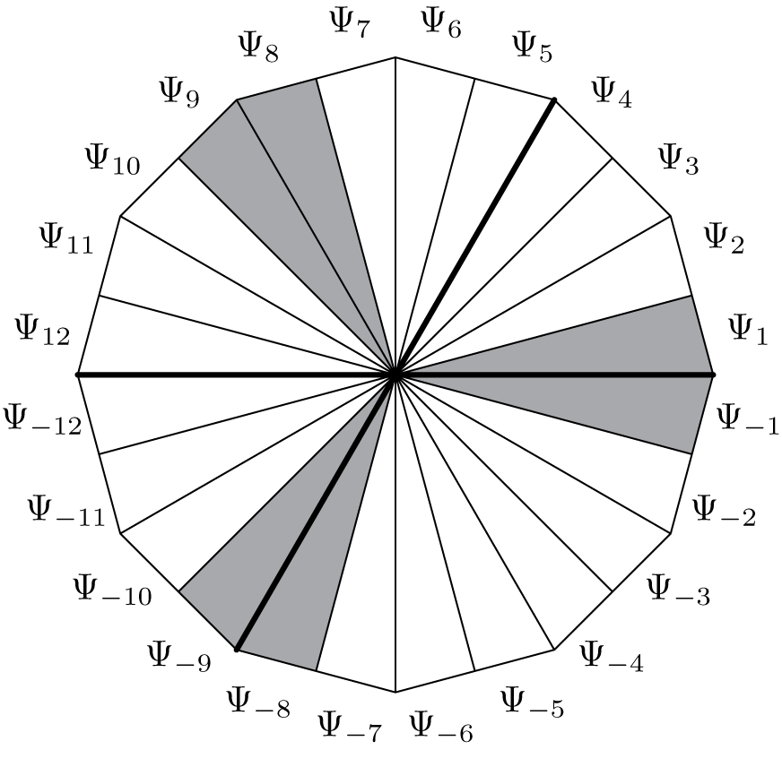
Theorem 7.4. Let
 $f\colon (\mathbb {C},0)\to (\mathbb {C},0)$
be an antiholomorphic parabolic germ of codimension k and of positive type when k is even. Let
$f\colon (\mathbb {C},0)\to (\mathbb {C},0)$
be an antiholomorphic parabolic germ of codimension k and of positive type when k is even. Let
 $(k, b, [\Psi _1,\ldots ,\Psi _k])$
be the modulus of f and let
$(k, b, [\Psi _1,\ldots ,\Psi _k])$
be the modulus of f and let
 $n\geq 3$
be an odd number. Then f has a single antiholomorphic formal nth root (n odd). Moreover, f has an antiholomorphic nth root (n odd) if and only if
$n\geq 3$
be an odd number. Then f has a single antiholomorphic formal nth root (n odd). Moreover, f has an antiholomorphic nth root (n odd) if and only if
 $$ \begin{align} \Psi_{j} \circ T_{{1/n}} = T_{{1/n}} \circ \Psi_{j}. \end{align} $$
Proof That f has a unique formal nth root follows from Proposition 3.4.
For the second part, f has an antiholomorphic nth root if and only if the transition functions satisfy
 $\Psi _{j} \circ \Sigma \circ T_{1/2n} = \Sigma \circ T_{1/2n}\circ \Psi _{-j}$
, since we may realize
$\Psi _{j} \circ \Sigma \circ T_{1/2n} = \Sigma \circ T_{1/2n}\circ \Psi _{-j}$
, since we may realize
 $\Sigma \circ T_{1/2n}$
on the Riemann surface of
$\Sigma \circ T_{1/2n}$
on the Riemann surface of
 $f\circ f$
. We combine this last equation with (15) to obtain
$f\circ f$
. We combine this last equation with (15) to obtain
 $\Psi _{j}\circ T_{(1/2n)-{(1/2)}} = T_{(1/2n)-{(1/2)}}\circ \Psi _{j}$
. To conclude, we note that
$\Psi _{j}\circ T_{(1/2n)-{(1/2)}} = T_{(1/2n)-{(1/2)}}\circ \Psi _{j}$
. To conclude, we note that
 $\gcd (1-n, 2n)=2$
because n is odd, so there exists
$\gcd (1-n, 2n)=2$
because n is odd, so there exists
 $p,q\in \mathbb {Z}$
such that
$p,q\in \mathbb {Z}$
such that
 $(1-n)p - 2nq\! =\! 2$
. In other words, we have
$(1-n)p - 2nq\! =\! 2$
. In other words, we have
 ${1/n}\! =\! ((1-n)/ 2n)p - q$
. Since
${1/n}\! =\! ((1-n)/ 2n)p - q$
. Since
 $\Psi _{j}$
commutes with
$\Psi _{j}$
commutes with
 $T_{{((1-n)/2n)}p}$
and with
$T_{{((1-n)/2n)}p}$
and with
 $T_q$
(because q is an integer), it follows that
$T_q$
(because q is an integer), it follows that
 $\Psi _{j}$
commutes with
$\Psi _{j}$
commutes with
 $T_{1/n}$
.
$T_{1/n}$
.
Corollary 7.5. f has an antiholomorphic nth root for n odd if and only if f is the square root of g and g has a holomorphic nth root with n odd.
Proof Equation (34) is independent of the representative and it is equivalent to a holomorphic parabolic germ having a holomorphic nth root (see [Reference Ilyashenko5]).
Suppose that
 $g = f\circ f$
and g has a holomorphic nth root. Then the modulus of g and f satisfies (34), so that f has an antiholomorphic nth root.
$g = f\circ f$
and g has a holomorphic nth root. Then the modulus of g and f satisfies (34), so that f has an antiholomorphic nth root.
The converse is direct.
7.3 Germs with an invariant real analytic curve
An antiholomorphic germ with real coefficients preserves the real axis. Any germ f analytically conjugate to the latter will preserve a real analytic curve; it is a property of the equivalence class of f. Therefore, Question 7.2 is equivalent to asking when does an antiholomorphic parabolic germ f preserve a real analytic curve?
Like the embedding problem, to preserve a germ of real axis is a condition of codimension infinity, but it is a ‘smaller’ infinity, that is, not every transition function needs to be a translation, but we will see that there are infinitely many conditions of the form
 $c_{n,j} = \overline {c_{-n,-j}}$
for the Fourier coefficients in (18).
$c_{n,j} = \overline {c_{-n,-j}}$
for the Fourier coefficients in (18).
Theorem 7.6. Let
 $f\colon (\mathbb {C},0)\to (\mathbb {C},0)$
be an antiholomorphic parabolic germ and
$f\colon (\mathbb {C},0)\to (\mathbb {C},0)$
be an antiholomorphic parabolic germ and
 $(k,b, [\Psi _1,\ldots ,\Psi _k])$
be its modulus of classification. The following statements are equivalent:
$(k,b, [\Psi _1,\ldots ,\Psi _k])$
be its modulus of classification. The following statements are equivalent:
-
(1) f preserves a real analytic curve at the origin;
-
(2) f is analytically conjugate to a germ with real coefficients;
-
(3) each representative
$(\Psi _1,\ldots ,\Psi _k)$
satisfies
$\Psi _j\circ {T_{\scriptscriptstyle {1/2}}} = {T_{\scriptscriptstyle {1/2}}} \circ \Psi _j$
; -
(4) each representative
$(\Psi _1,\ldots ,\Psi _k)$
satisfies
$\Psi _j\circ \Sigma = \Sigma \circ \Psi _{-j}$
, where
$\Psi _{-j}$
is defined by (
17
).


Proof (1)
 $\Rightarrow $
(2) Let
$\Rightarrow $
(2) Let
 $\gamma $
be the germ of real analytic parametrization of the invariant curve of f. We can extend
$\gamma $
be the germ of real analytic parametrization of the invariant curve of f. We can extend
 $\gamma $
on a disk around the origin. Then
$\gamma $
on a disk around the origin. Then
 $\gamma ^{-1}\circ f\circ \gamma $
fixes a germ of the real axis, so its power series has real coefficients.
$\gamma ^{-1}\circ f\circ \gamma $
fixes a germ of the real axis, so its power series has real coefficients.
(2)
 $\Rightarrow $
(3) We can of course suppose that the power series of f has real coefficients, so that
$\Rightarrow $
(3) We can of course suppose that the power series of f has real coefficients, so that
 $\sigma \circ f = f\circ \sigma $
. It follows that
$\sigma \circ f = f\circ \sigma $
. It follows that
 $\sigma \circ f$
is a holomorphic square root of
$\sigma \circ f$
is a holomorphic square root of
 $g = f\circ f$
. Therefore, we have
$g = f\circ f$
. Therefore, we have
 $\Psi _j\circ {T_{\scriptscriptstyle {1/2}}} = {T_{\scriptscriptstyle {1/2}}} \circ \Psi _j$
.
$\Psi _j\circ {T_{\scriptscriptstyle {1/2}}} = {T_{\scriptscriptstyle {1/2}}} \circ \Psi _j$
.
(3)
 $\Leftrightarrow $
(4) It follows from equation (15).
$\Leftrightarrow $
(4) It follows from equation (15).
(4)
 $\Rightarrow $
(1) This is the harder part of the proof. The hypothesis implies that
$\Rightarrow $
(1) This is the harder part of the proof. The hypothesis implies that
 $\Sigma $
is well defined on the Riemann surface S constructed in the proof of part (2) of the classification theorem (Theorem 6.3). Let
$\Sigma $
is well defined on the Riemann surface S constructed in the proof of part (2) of the classification theorem (Theorem 6.3). Let
 $z = H(W)$
be the coordinate given by
$z = H(W)$
be the coordinate given by
 $H\colon S\to (\mathbb {C},0)\setminus \{0\}$
, the biholomorphism of S to a punctured neighbourhood of the origin. Let
$H\colon S\to (\mathbb {C},0)\setminus \{0\}$
, the biholomorphism of S to a punctured neighbourhood of the origin. Let
 $\sigma '$
and
$\sigma '$
and
 $f'$
be the expressions of
$f'$
be the expressions of
 $\Sigma $
and
$\Sigma $
and
 $\Sigma \circ {T_{\scriptscriptstyle {1/2}}}$
in this coordinate (note that f and
$\Sigma \circ {T_{\scriptscriptstyle {1/2}}}$
in this coordinate (note that f and
 $f'$
are analytically conjugate). Since, on S,
$f'$
are analytically conjugate). Since, on S,
 $\Sigma $
and
$\Sigma $
and
 $\Sigma \circ {T_{\scriptscriptstyle {1/2}}}$
commute, it follows that
$\Sigma \circ {T_{\scriptscriptstyle {1/2}}}$
commute, it follows that
 $\sigma '$
and
$\sigma '$
and
 $f'$
commute also. So, it remains only to show that
$f'$
commute also. So, it remains only to show that
 $\sigma '$
preserves a germ of real analytic curve at the origin.
$\sigma '$
preserves a germ of real analytic curve at the origin.
We can extend
 $\sigma '$
by
$\sigma '$
by
 $\sigma '(0) = 0$
by the Riemann removable singularity theorem (this is true for antiholomorphic functions, since we simply apply it to
$\sigma '(0) = 0$
by the Riemann removable singularity theorem (this is true for antiholomorphic functions, since we simply apply it to
 $\sigma '\circ \sigma $
, where
$\sigma '\circ \sigma $
, where
 $\sigma (z) = {\overline z}$
). In the charts
$\sigma (z) = {\overline z}$
). In the charts
 $U_0$
and
$U_0$
and
 $U_k$
,
$U_k$
,
 $\Sigma $
fixes the real axis. These two curves carry in the z-coordinate and meet at the origin to form a continuous curve
$\Sigma $
fixes the real axis. These two curves carry in the z-coordinate and meet at the origin to form a continuous curve
 $\gamma $
fixed by
$\gamma $
fixed by
 $\sigma '$
. In fact,
$\sigma '$
. In fact,
 $\gamma $
is a
$\gamma $
is a
 $C^1$
curve, as H can be extended to a
$C^1$
curve, as H can be extended to a
 $C^1$
diffeomorphism
$C^1$
diffeomorphism
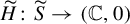 $\widetilde H\colon \widetilde S\to (\mathbb {C},0)$
, where
$\widetilde H\colon \widetilde S\to (\mathbb {C},0)$
, where
 $\widetilde S$
is obtained from S with the point
$\widetilde S$
is obtained from S with the point
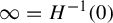 $\infty = H^{-1}(0)$
added.
$\infty = H^{-1}(0)$
added.
This curve divides a small disk
 $D(0,\delta )$
into two connected components A and B. By the Riemann mapping theorem, there exists a biholomorphism
$D(0,\delta )$
into two connected components A and B. By the Riemann mapping theorem, there exists a biholomorphism
 $\varphi $
of A to the upper half-plane that sends continuously the boundary of A on the real line; see Figure 19. The image of
$\varphi $
of A to the upper half-plane that sends continuously the boundary of A on the real line; see Figure 19. The image of
 $\gamma $
corresponds to an interval
$\gamma $
corresponds to an interval
 $[a,b]$
. We can extend
$[a,b]$
. We can extend
 $\varphi $
to
$\varphi $
to
 $A\cup \gamma \cup B$
by
$A\cup \gamma \cup B$
by
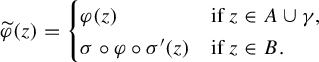 $$ \begin{align*}\widetilde\varphi(z) =\begin{cases} \varphi(z) & \textrm{if } z\in A\cup\gamma,\\ \sigma\circ\varphi\circ\sigma'(z) & \textrm{if } z\in B. \end{cases} \end{align*} $$
This is holomorphic on B, since it is the composition of a holomorphic map with two antiholomorphic maps, and it is continuous on
 $A\cup \gamma \cup B$
.
$A\cup \gamma \cup B$
.
Mapping
 $\varphi $
extended on
$\varphi $
extended on
 $A\cup \gamma \cup B$
.
$A\cup \gamma \cup B$
.
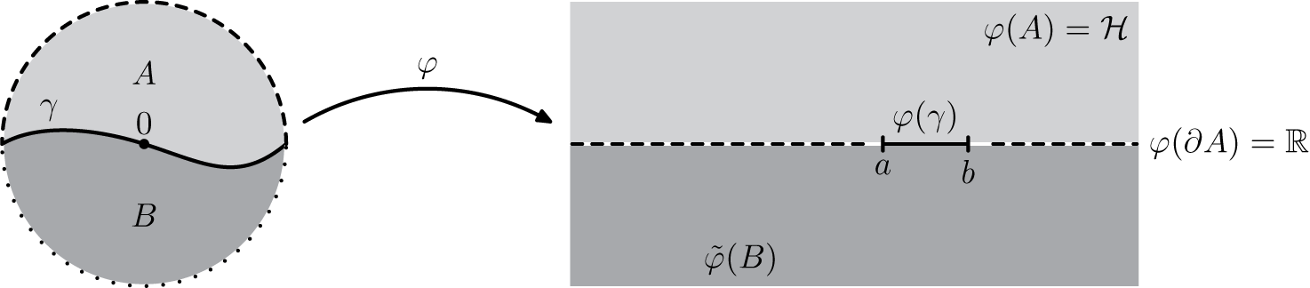
The argument to prove that
 $\widetilde \varphi $
is holomorphic is similar to that of the Schwarz reflection principle. The idea is to show that the integral of
$\widetilde \varphi $
is holomorphic is similar to that of the Schwarz reflection principle. The idea is to show that the integral of
 $\widetilde \varphi $
along any triangle in
$\widetilde \varphi $
along any triangle in
 $A\cup \gamma \cup B$
vanishes, and it will then follow from Morera’s theorem. If a simple closed curve is in
$A\cup \gamma \cup B$
vanishes, and it will then follow from Morera’s theorem. If a simple closed curve is in
 $A\cup \gamma $
or
$A\cup \gamma $
or
 $B\cup \gamma $
, then it follows from Cauchy’s theorem (we may take a limit of closed curves in A or B converging to the initial one). Then we can divide any triangle in
$B\cup \gamma $
, then it follows from Cauchy’s theorem (we may take a limit of closed curves in A or B converging to the initial one). Then we can divide any triangle in
 $A\cup \gamma \cup B$
along
$A\cup \gamma \cup B$
along
 $\gamma $
to obtain a finite number of closed curves in
$\gamma $
to obtain a finite number of closed curves in
 $A\cup \gamma $
and in
$A\cup \gamma $
and in
 $B\cup \gamma $
, as in Figure 20. Thus,
$B\cup \gamma $
, as in Figure 20. Thus,
 $\widetilde \varphi |_{(a,b)}^{-1}$
is a real analytic parametrization of
$\widetilde \varphi |_{(a,b)}^{-1}$
is a real analytic parametrization of
 $\gamma $
.
$\gamma $
.
Triangle divided into two closed curves.
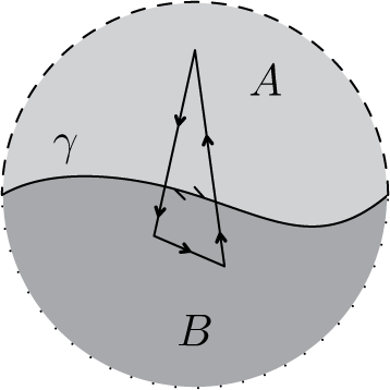
When f is conjugate to a germ with real coefficients, then so is the holomorphic germ
 $g = f\circ f$
. However, it is not true that every holomorphic germ analytically conjugate to a germ with real coefficients must have a germ f such that
$g = f\circ f$
. However, it is not true that every holomorphic germ analytically conjugate to a germ with real coefficients must have a germ f such that
 $g = f\circ f$
, as the next theorem will show (see also Proposition 7.8). Even though this is not a property directly linked to the antiholomorphic parabolic germs, we will still prove the following necessary and sufficient condition for a holomorphic parabolic germ to preserve a real analytic curve.
$g = f\circ f$
, as the next theorem will show (see also Proposition 7.8). Even though this is not a property directly linked to the antiholomorphic parabolic germs, we will still prove the following necessary and sufficient condition for a holomorphic parabolic germ to preserve a real analytic curve.
Theorem 7.7. Let
 $g\colon (\mathbb {C},0) \to (\mathbb {C},0)$
be a parabolic holomorphic germ and let
$g\colon (\mathbb {C},0) \to (\mathbb {C},0)$
be a parabolic holomorphic germ and let
 $(k,b, [\Psi _{-k},\ldots ,\Psi _{-1},\Psi _1,\ldots ,\Psi _k])$
be its Écalle–Voronin modulus (see §5.1). The following statements are equivalent:
$(k,b, [\Psi _{-k},\ldots ,\Psi _{-1},\Psi _1,\ldots ,\Psi _k])$
be its Écalle–Voronin modulus (see §5.1). The following statements are equivalent:
-
(1) g preserves a germ of real analytic curve at the origin;
-
(2) g is analytically conjugate to a germ with real coefficients;
-
(3) for each representative
$(\Psi _{-k},\ldots ,\Psi _{-1},\Psi _1,\ldots ,\Psi _k)$
, there exists
$y\in \mathbb {R}$
such that the transition functions satisfy
$\Sigma \circ T_{iy}\circ \Psi _{j} = \Psi _{-j}\circ \Sigma \circ T_{iy}$
; -
(4) there exists a representative
$(\Psi _{-k},\ldots ,\Psi _{-1},\Psi _1,\ldots ,\Psi _k)$
such that
$\Psi _{j}\circ \Sigma = \Sigma \circ \Psi _{-j}$
.


Proof (1)
 $\Rightarrow $
(2) and (4)
$\Rightarrow $
(2) and (4)
 $\Rightarrow $
(1) are the same as in the previous theorem.
$\Rightarrow $
(1) are the same as in the previous theorem.
(2)
 $\Rightarrow $
(3) Suppose that g is in a coordinate such that
$\Rightarrow $
(3) Suppose that g is in a coordinate such that
 $g = \sigma \circ g\circ \sigma $
. Let
$g = \sigma \circ g\circ \sigma $
. Let
 $\Phi _j$
be a Fatou coordinate on
$\Phi _j$
be a Fatou coordinate on
 $U_j$
for
$U_j$
for
 $-k \leq j\leq k$
, where
$-k \leq j\leq k$
, where
 $\Phi _{-k} = \Phi _k$
. Then
$\Phi _{-k} = \Phi _k$
. Then
 $\Sigma \circ \Phi _{-j}\circ \Sigma $
is also a Fatou coordinate of g on
$\Sigma \circ \Phi _{-j}\circ \Sigma $
is also a Fatou coordinate of g on
 $U_j$
. By the uniqueness of the Fatou coordinate (for the holomorphic case), there exists a constant
$U_j$
. By the uniqueness of the Fatou coordinate (for the holomorphic case), there exists a constant
 $C\in \mathbb {C}$
such that
$C\in \mathbb {C}$
such that
 $$ \begin{align*}\Sigma\circ \Phi_{-j}\circ\Sigma\circ \Phi_j^{-1} = T_C \end{align*} $$
for all j. In particular, for
 $j=0$
, by taking the inverse and conjugating both sides by
$j=0$
, by taking the inverse and conjugating both sides by
 $\Sigma $
of the previous equation, we obtain
$\Sigma $
of the previous equation, we obtain
 $T_C = T_{-\overline C}$
, so C must be pure imaginary, say
$T_C = T_{-\overline C}$
, so C must be pure imaginary, say
 $iy$
with
$iy$
with
 $y\in \mathbb {R}$
. For
$y\in \mathbb {R}$
. For
 $j>0$
and odd, we conclude with
$j>0$
and odd, we conclude with
 $$ \begin{align*}\displaystyle\Psi_j = \Phi_j\circ \Phi_{j-1}^{-1} = T_{-iy}\circ \Sigma \circ \Phi_{-j} \circ \Phi_{-j+1}^{-1}\circ \Sigma\circ T_{iy} = T_{-iy}\circ \Sigma \circ \Psi_{-j} \circ \Sigma\circ T_{iy}. \end{align*} $$
The other values of j are done similarly.
(3)
 $\Leftrightarrow $
(4) It follows from the fact that for any two representatives
$\Leftrightarrow $
(4) It follows from the fact that for any two representatives
 $(\Psi _{-k},\ldots ,\Psi _{-1}, \Psi _1,\ldots , \Psi _k)$
and
$(\Psi _{-k},\ldots ,\Psi _{-1}, \Psi _1,\ldots , \Psi _k)$
and
 $(\Psi _{-k}',\ldots ,\Psi _{-1}',\Psi _1',\ldots ,\Psi _k')$
, there exists
$(\Psi _{-k}',\ldots ,\Psi _{-1}',\Psi _1',\ldots ,\Psi _k')$
, there exists
 $C\in \mathbb {C}$
such that
$C\in \mathbb {C}$
such that
 $\Psi _j\circ T_C = T_C \circ \Psi _j'$
. We choose
$\Psi _j\circ T_C = T_C \circ \Psi _j'$
. We choose
 $C = -{iy/2}$
to get a representative satisfying
$C = -{iy/2}$
to get a representative satisfying
 $\Psi _j'\circ \Sigma = \Sigma \circ \Psi _{-j}'$
.
$\Psi _j'\circ \Sigma = \Sigma \circ \Psi _{-j}'$
.
Proposition 7.8. There exists g with real coefficients that has no antiholomorphic square root (see §7.2).
Proof The holomorphic germ realized by the Écalle–Voronin modulus
 $(1,0,[W + e^{2i\pi W}, W + e^{-2i\pi W}])$
has no antiholomorphic square root, but preserves a germ of real analytic curve.
$(1,0,[W + e^{2i\pi W}, W + e^{-2i\pi W}])$
has no antiholomorphic square root, but preserves a germ of real analytic curve.
7.4 Centralizer in the group of holomorphic and antiholomorphic germs
Let
 $\mathop {\mathrm {Diff}}\nolimits _1(0, \mathbb {C})$
(respectively
$\mathop {\mathrm {Diff}}\nolimits _1(0, \mathbb {C})$
(respectively
 $\overline {\mathop {\mathrm {Diff}}\nolimits _1(0,\mathbb {C})}$
) be the set of germs of holomorphic (respectively antiholomorphic) diffeomorphisms with a fixed point at the origin with multiplier 1. Note in particular that an antiholomorphic germ must be tangent to
$\overline {\mathop {\mathrm {Diff}}\nolimits _1(0,\mathbb {C})}$
) be the set of germs of holomorphic (respectively antiholomorphic) diffeomorphisms with a fixed point at the origin with multiplier 1. Note in particular that an antiholomorphic germ must be tangent to
 $\sigma $
. We set
$\sigma $
. We set
 $$ \begin{align*}\mathop{\mathrm{Diff}}\nolimits_1(0,\mathbb{C},\overline{\mathbb{C}}) = \mathop{\mathrm{Diff}}\nolimits_1(0,\mathbb{C})\cup \overline{\mathop{\mathrm{Diff}}\nolimits_1(0,\mathbb{C})}. \end{align*} $$
It forms a group with
 $\mathop {\mathrm {Diff}}\nolimits _1(0,\mathbb {C})$
as a subgroup. Next, let
$\mathop {\mathrm {Diff}}\nolimits _1(0,\mathbb {C})$
as a subgroup. Next, let
 $\mathcal A_{k,b}\subset \mathop {\mathrm {Diff}}\nolimits _1(0,\mathbb {C})$
(respectively
$\mathcal A_{k,b}\subset \mathop {\mathrm {Diff}}\nolimits _1(0,\mathbb {C})$
(respectively
 $\overline {\mathcal A_{k,b}}\subset \overline {\mathop {\mathrm {Diff}}\nolimits _1(0,\mathbb {C})}$
when b is real) be the set of germs of holomorphic (respectively antiholomorphic) diffeomorphisms with a parabolic fixed point of codimension k at the origin and with formal invariant b.
$\overline {\mathcal A_{k,b}}\subset \overline {\mathop {\mathrm {Diff}}\nolimits _1(0,\mathbb {C})}$
when b is real) be the set of germs of holomorphic (respectively antiholomorphic) diffeomorphisms with a parabolic fixed point of codimension k at the origin and with formal invariant b.
We will study the centralizer of
 $g\in \mathcal A_{k,b}$
and of
$g\in \mathcal A_{k,b}$
and of
 $f\in \overline {\mathcal A_{k,b}}$
in
$f\in \overline {\mathcal A_{k,b}}$
in
 $\mathop {\mathrm {Diff}}\nolimits _1(0,\mathbb {C},\overline {\mathbb {C}})$
. Let us note the following: if
$\mathop {\mathrm {Diff}}\nolimits _1(0,\mathbb {C},\overline {\mathbb {C}})$
. Let us note the following: if
 $g\in \mathcal A_{k,b}$
commutes with
$g\in \mathcal A_{k,b}$
commutes with
 $f\in \overline {\mathop {\mathrm {Diff}}\nolimits _1(0,\mathbb {C})}$
, then the formal invariant b of g is automatically real. In fact, we have that g and
$f\in \overline {\mathop {\mathrm {Diff}}\nolimits _1(0,\mathbb {C})}$
, then the formal invariant b of g is automatically real. In fact, we have that g and
 $\sigma \circ g\circ \sigma $
are analytically conjugate by means of
$\sigma \circ g\circ \sigma $
are analytically conjugate by means of
 $(\sigma \circ f)$
. So, we are interested only in b real, since, if b is not real, the centralizer of g in
$(\sigma \circ f)$
. So, we are interested only in b real, since, if b is not real, the centralizer of g in
 $\mathop {\mathrm {Diff}}\nolimits _1(0,\mathbb {C},\overline {\mathbb {C}})$
is the same as the centralizer of g in
$\mathop {\mathrm {Diff}}\nolimits _1(0,\mathbb {C},\overline {\mathbb {C}})$
is the same as the centralizer of g in
 $\mathop {\mathrm {Diff}}\nolimits (0,\mathbb {C})$
, which is already known (see [Reference Ilyashenko5]).
$\mathop {\mathrm {Diff}}\nolimits (0,\mathbb {C})$
, which is already known (see [Reference Ilyashenko5]).
Lemma 7.9. Let
 $g\in \mathcal A_{k,b}$
and let
$g\in \mathcal A_{k,b}$
and let
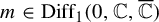 $m\in \mathop {\mathrm {Diff}}\nolimits _1(0,\mathbb {C},\overline {\mathbb {C}})$
be a germ that commutes with
$m\in \mathop {\mathrm {Diff}}\nolimits _1(0,\mathbb {C},\overline {\mathbb {C}})$
be a germ that commutes with
 $g\in \mathcal A_{k,b}$
. Then m is the identity, or analytically conjugate to
$g\in \mathcal A_{k,b}$
. Then m is the identity, or analytically conjugate to
 $\sigma $
, or
$\sigma $
, or
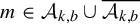 $m\in \mathcal A_{k,b}\cup \overline {\mathcal A_{k,b}}$
. Moreover, in the Fatou coordinates of g, m will be of the form
$m\in \mathcal A_{k,b}\cup \overline {\mathcal A_{k,b}}$
. Moreover, in the Fatou coordinates of g, m will be of the form
 $$ \begin{align} T_C \quad\textrm{or}\quad \Sigma\circ T_C \qquad\textrm{for }C\in\mathbb{C}. \end{align} $$
Proof If m is not the identity or analytically conjugate to
 $\sigma $
, then m is parabolic. It must have codimension k, since it maps the orbits of g on the orbits of g and the Fatou petals of g on the Fatou petals of g. To see that m has the same formal invariant, we compare degree by degree the power series on both sides of the equation
$\sigma $
, then m is parabolic. It must have codimension k, since it maps the orbits of g on the orbits of g and the Fatou petals of g on the Fatou petals of g. To see that m has the same formal invariant, we compare degree by degree the power series on both sides of the equation
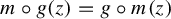 $m\circ g(z) = g\circ m(z)$
.
$m\circ g(z) = g\circ m(z)$
.
To see that m has one of the forms of (35), the first part of the proof of Proposition 4.5 applies almost identically to m.
The obvious germs in the centralizer of f or g are the iterates, the roots, and the iterates of the roots, which we define below as the fractional iterates. We prove in Theorems 7.11 and 7.12 that these are all the possible elements of the centralizer, provided that f or g are not conjugate to their respective normal forms.
Definition 7.10. Let
 $f\in \overline {\mathcal A_{k,b}}$
(respectively
$f\in \overline {\mathcal A_{k,b}}$
(respectively
 $g\in \mathcal A_{k,b}$
). We say that
$g\in \mathcal A_{k,b}$
). We say that
 $m\in \mathop {\mathrm {Diff}}\nolimits _1(0,\mathbb {C},\overline {\mathbb {C}})$
is a fractional iterate of order p of f (respectively g) if there exists
$m\in \mathop {\mathrm {Diff}}\nolimits _1(0,\mathbb {C},\overline {\mathbb {C}})$
is a fractional iterate of order p of f (respectively g) if there exists
 $q\in \mathbb {Z}$
such that
$q\in \mathbb {Z}$
such that
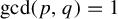 $\gcd (p,q)=1$
and
$\gcd (p,q)=1$
and
 $m^{\circ p} = f^{\circ q}$
(respectively
$m^{\circ p} = f^{\circ q}$
(respectively
 $m^{\circ p} = g^{\circ q}$
).
$m^{\circ p} = g^{\circ q}$
).
Note that a fractional iterate of order one is just an iterate of f or of g.
Theorem 7.11. Let
 $g\in \mathcal A_{k,b}$
with
$g\in \mathcal A_{k,b}$
with
 $b\in \mathbb {R}$
. Then we have one of the following cases.
$b\in \mathbb {R}$
. Then we have one of the following cases.
-
(1) g is embeddable, that is,
$g = h\circ v^{\scriptscriptstyle 1}\circ h^{-1}$
. Let
$g_t = h\circ v^t\circ h^{-1}$
. Then the centralizer of g is
$$ \begin{align*}Z_{g} = \{g_t \mid t\in\mathbb{C}\}\cup \{h\circ \sigma\circ v^t\circ h^{-1}\mid t\in\mathbb{C}\}. \end{align*} $$
-
(2) g is not embeddable; then
$Z_g$
contains only holomorphic and antiholomorphic fractional iterates of g and Schwarz reflections. More precisely, there exists
$p\in \mathbb {N}\setminus \{0\}$
such that the centralizer of g is one of the following:-
•
$ \begin {aligned}\hspace{-13pt} Z_g = \bigcup _{d\mid p}\,\{\text {fractional iterates of order }d \text {of} g\}; \end {aligned} $
-
•
$ \begin {aligned}\hspace{-15pt} Z_g &= \bigcup _{d\mid p}\, \{\text {hol. fractional iterates of order }d \text {of} g\} {}\\ &\quad \cup \bigcup _{d\mid 2p\atop d\,\textit {even}} \{\text {antihol. fractional iterates of order }d \text {of} g\}; \end {aligned} $
-
•
$ \begin {aligned}\hspace{-15pt} Z_g &= \bigcup _{d\mid p}\, \{\text {hol. fractional iterates of order }d \text {of} g\} {}\\ &\quad \cup \bigcup _{d\mid p\atop d\,\textit {even}} \{\text {antihol. fractional iterates of order }d \text {of} g\}\\ &\quad \cup \{\text {Schwarz reflection tangent to }\sigma \}. \end {aligned} $
The centralizer includes a Schwarz reflection tangent to
$\sigma $
if and only if g is analytically conjugate to a germ with real coefficients (see Theorem 7.7). -


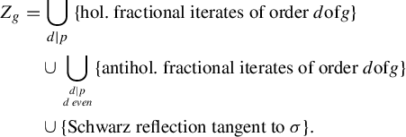

Proof (1) Since g is embeddable, each of its transition functions is a translation, so any
 $T_t$
will commute with them. Each
$T_t$
will commute with them. Each
 $T_t$
represents a germ analytically conjugate to
$T_t$
represents a germ analytically conjugate to
 $g^t$
for some
$g^t$
for some
 $t\in \mathbb {C}$
. In the case where m is antiholomorphic,
$t\in \mathbb {C}$
. In the case where m is antiholomorphic,
 $\Sigma \circ T_t$
is compatible with the transition functions with no restriction on t. It corresponds to
$\Sigma \circ T_t$
is compatible with the transition functions with no restriction on t. It corresponds to
 $h\circ \sigma \circ v^{t}\circ h^{-1}$
for
$h\circ \sigma \circ v^{t}\circ h^{-1}$
for
 $t\in \mathbb {C}$
.
$t\in \mathbb {C}$
.
(2) Since g is not embeddable, one of the transition functions is not a translation. Suppose that
 $g_1\in \mathop {\mathrm {Diff}}\nolimits _1(0,\mathbb {C},\overline {\mathbb {C}})$
is holomorphic and commutes with g. By Lemma 7.9,
$g_1\in \mathop {\mathrm {Diff}}\nolimits _1(0,\mathbb {C},\overline {\mathbb {C}})$
is holomorphic and commutes with g. By Lemma 7.9,
 $g_1$
becomes
$g_1$
becomes
 $T_t$
in the Fatou coordinates for some
$T_t$
in the Fatou coordinates for some
 $t\in \mathbb {C}$
. Then
$t\in \mathbb {C}$
. Then
 $T_t$
must commute with the transition functions. This will only happen if the transition functions expand in the form
$T_t$
must commute with the transition functions. This will only happen if the transition functions expand in the form
 $$ \begin{align} \Psi_j(W) = W + (-1)^j{i\pi b\over k} + \sum_{\ell\in\mathbb{Z}^\ast} c_{\ell p,j}e^{2i\pi \ell p W} \end{align} $$
and
 $t = {a/p}$
for some
$t = {a/p}$
for some
 $a,p\in \mathbb {N}$
. This corresponds to
$a,p\in \mathbb {N}$
. This corresponds to
 $g_1$
being a holomorphic fractional iterate of order p of g. Let p denote the maximal order of holomorphic roots of g.
$g_1$
being a holomorphic fractional iterate of order p of g. Let p denote the maximal order of holomorphic roots of g.
Suppose that
 $f_1\in \mathop {\mathrm {Diff}}\nolimits _1(0,\mathbb {C},\overline {\mathbb {C}})$
is antiholomorphic and commutes with g. We can suppose that
$f_1\in \mathop {\mathrm {Diff}}\nolimits _1(0,\mathbb {C},\overline {\mathbb {C}})$
is antiholomorphic and commutes with g. We can suppose that
 $f_1$
is not a Schwarz reflection, since this is covered in Theorem 7.7. Then, by Lemma 7.9,
$f_1$
is not a Schwarz reflection, since this is covered in Theorem 7.7. Then, by Lemma 7.9,
 $f_1$
is
$f_1$
is
 $\Sigma \circ T_{\scriptscriptstyle t}$
in the Fatou coordinates and it must be compatible with the transition functions. Therefore,
$\Sigma \circ T_{\scriptscriptstyle t}$
in the Fatou coordinates and it must be compatible with the transition functions. Therefore,
 $T_{2\Re t}$
commutes with the
$T_{2\Re t}$
commutes with the
 $\Psi _j$
and, by the previous case, we have
$\Psi _j$
and, by the previous case, we have
 $2\Re t = {a / r}$
with
$2\Re t = {a / r}$
with
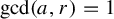 $\gcd (a,r) = 1$
and
$\gcd (a,r) = 1$
and
 $r\,|\, p$
. We have
$r\,|\, p$
. We have
 $\Sigma \circ T_{\scriptscriptstyle t}\circ \Psi _j = \Psi _{-j}\circ \Sigma \circ T_{\scriptscriptstyle t}$
for some representative of the modulus if and only if
$\Sigma \circ T_{\scriptscriptstyle t}\circ \Psi _j = \Psi _{-j}\circ \Sigma \circ T_{\scriptscriptstyle t}$
for some representative of the modulus if and only if
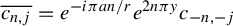 $$ \begin{align} \overline{c_{n,j}} = e^{-i\pi an/r}e^{2n\pi y}c_{-n,-j} \end{align} $$
and
 $t = (a/2r) + iy$
(
$t = (a/2r) + iy$
(
 $y\in \mathbb {R}$
), where
$y\in \mathbb {R}$
), where
 $c_{n,j}$
are the Fourier coefficients of
$c_{n,j}$
are the Fourier coefficients of
 $\Psi _j$
from (18). Of course, generically there exists no y that satisfy (37), so there are no antiholomorphic germs that commute with g in the generic case. When such a y exists, by changing the
$\Psi _j$
from (18). Of course, generically there exists no y that satisfy (37), so there are no antiholomorphic germs that commute with g in the generic case. When such a y exists, by changing the
 $\Psi _j$
by
$\Psi _j$
by
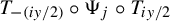 $T_{-{(iy/2)}}\circ \Psi _j\circ T_{{iy/2}}$
, we can suppose that
$T_{-{(iy/2)}}\circ \Psi _j\circ T_{{iy/2}}$
, we can suppose that
 $y=0$
.
$y=0$
.
Since
 ${T_{\scriptscriptstyle {1/ p}}}$
commutes with the
${T_{\scriptscriptstyle {1/ p}}}$
commutes with the
 $\Psi _j$
, we have
$\Psi _j$
, we have
 $c_{n,j} = 0$
if
$c_{n,j} = 0$
if
 $p{\kern-4pt}\not{\kern0.9pt}|{\kern0.8pt}n$
, so that (37) becomes
$p{\kern-4pt}\not{\kern0.9pt}|{\kern0.8pt}n$
, so that (37) becomes
 $\overline {c_{sp,j}} = e^{-i\pi s ap/r} c_{-sp,-j}$
.
$\overline {c_{sp,j}} = e^{-i\pi s ap/r} c_{-sp,-j}$
.
If
 $p/r$
and a are odd, then (37) becomes
$p/r$
and a are odd, then (37) becomes
 $$ \begin{align*}\overline{c_{sp,j}} = \begin{cases} -c_{sp,j}, & s \textrm{ odd,}\\ c_{sp,j}, & s \textrm{ even.} \end{cases} \end{align*} $$
This is precisely the condition for g to have an antiholomorphic root of order
 $2p$
.
$2p$
.
If
 $p/r$
or a is even, then
$p/r$
or a is even, then
 $e^{-i\pi asp/r} = 1$
for all s, so we obtain the condition necessary for
$e^{-i\pi asp/r} = 1$
for all s, so we obtain the condition necessary for
 $\Sigma $
to be compatible with the transition functions and then there is a Schwarz reflection in the centralizer of g. In that case, the highest orders of the holomorphic and antiholomorphic iterates coincide.
$\Sigma $
to be compatible with the transition functions and then there is a Schwarz reflection in the centralizer of g. In that case, the highest orders of the holomorphic and antiholomorphic iterates coincide.
Lastly, we will study the centralizer of
 $f\in \overline {\mathcal A_{k,b}}$
in
$f\in \overline {\mathcal A_{k,b}}$
in
 $\mathop {\mathrm {Diff}}\nolimits _1(0,\mathbb {C},\overline {\mathbb {C}})$
. Of course, we have
$\mathop {\mathrm {Diff}}\nolimits _1(0,\mathbb {C},\overline {\mathbb {C}})$
. Of course, we have
 $Z_f \subseteq Z_{f\circ f}$
, so the details are similar to the previous theorem.
$Z_f \subseteq Z_{f\circ f}$
, so the details are similar to the previous theorem.
Theorem 7.12. Let
 $f\in \overline {\mathcal A_{k,b}}$
. Then we have one of the following cases:
$f\in \overline {\mathcal A_{k,b}}$
. Then we have one of the following cases:
-
(1) f is embeddable, that is, if
$f = h\circ \sigma \circ v^{\scriptscriptstyle {1/2}}\circ h^{-1}$
, then its centralizer is
$$ \begin{align*}Z_{f} = \{h\circ v^t\circ h^{-1}\,|\, t\in\mathbb{R}\} \cup \{h\circ \sigma\circ v^{t}\circ h^{-1}\,|\, t\in\mathbb{R}\}; \end{align*} $$
-
(2) f is not embeddable; then
$Z_f$
contains only holomorphic and antiholomorphic fractional iterates of f and Schwarz reflections. More precisely, there exists
$p\in \mathbb {N}\setminus \{0\}$
such that the centralizer of f is one of the following:-
• if p is odd, then
$$ \begin{align*} \hspace{-9pc} \begin {aligned} Z_f &= \bigcup _{d\mid p}\, \{\text {hol. fractional iterates of order }d \text {of} f\circ f\}{}\\ &\quad \cup \bigcup _{d\mid p\atop d\,\textit {odd}} \{\text {antihol. fractional iterates of order }d \text {of} f\};\end {aligned} \end{align*} $$
-
• if p is even, then
$$ \begin{align*} \hspace{-9pc} \begin {aligned} Z_f &= \bigcup _{d\mid p}\, \{\text {hol. fractional iterates of order }d \text {of} f\circ f\}{}\\ &\quad \cup \bigcup _{d\mid p\atop d\,\textit {odd}} \{\text {antihol. fractional iterates of order }d \text {of} f\};\\ &\quad \cup \{\text {Schwarz reflection tangent to }\sigma \}. \end {aligned} \end{align*} $$
The centralizer includes a Schwarz reflection tangent to
$\sigma $
if and only if f is analytically conjugate to a germ with real coefficients (see Theorem 7.6). -


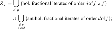
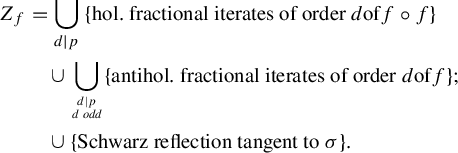

Proof (1) In the Fatou coordinates,
 $T_t$
must commute with
$T_t$
must commute with
 $\Sigma \circ {T_{\scriptscriptstyle {1/2}}}$
, so t must be real. The rest of the details are exactly as in the proof of Theorem 7.11.
$\Sigma \circ {T_{\scriptscriptstyle {1/2}}}$
, so t must be real. The rest of the details are exactly as in the proof of Theorem 7.11.
(2) Let
 $p\in \mathbb {N}$
be the highest order of the holomorphic roots of
$p\in \mathbb {N}$
be the highest order of the holomorphic roots of
 $f\circ f$
. This number might be one, in which case
$f\circ f$
. This number might be one, in which case
 $Z_f$
contains only iterates of f. Indeed, if
$Z_f$
contains only iterates of f. Indeed, if
 $p=1$
,
$p=1$
,
 $Z_f$
does not contain a Schwarz reflection, otherwise
$Z_f$
does not contain a Schwarz reflection, otherwise
 $f\circ f$
would have the holomorphic root
$f\circ f$
would have the holomorphic root
 $\sigma \circ f$
, which would contradict that the highest order of the holomorphic root is one. Let us suppose that
$\sigma \circ f$
, which would contradict that the highest order of the holomorphic root is one. Let us suppose that
 $p>1$
.
$p>1$
.
Let
 $(\Psi _1,\ldots ,\Psi _k)$
be a representative of the analytic invariant of f. Let
$(\Psi _1,\ldots ,\Psi _k)$
be a representative of the analytic invariant of f. Let
 $\Psi _{-j}$
be determined by (17) for
$\Psi _{-j}$
be determined by (17) for
 $j=1,\ldots ,k$
. Suppose that the transition functions have a Fourier expansion
$j=1,\ldots ,k$
. Suppose that the transition functions have a Fourier expansion
 $$ \begin{align*}\Psi_j(W) = W + C_j + \sum_{n} c_{n,j}e^{2i\pi nW} \end{align*} $$
for all j, where
 $\overline {C_{-j}} = C_j = (-1)^{j(i\pi b/k)}$
for
$\overline {C_{-j}} = C_j = (-1)^{j(i\pi b/k)}$
for
 $j>0$
. Because the
$j>0$
. Because the
 $\Psi _j$
satisfy
$\Psi _j$
satisfy
 $\Psi _j\circ \Sigma \circ {T_{\scriptscriptstyle {1/2}}} = \Sigma \circ {T_{\scriptscriptstyle {1/2}}} \circ \Psi _{-j}$
, we obtain
$\Psi _j\circ \Sigma \circ {T_{\scriptscriptstyle {1/2}}} = \Sigma \circ {T_{\scriptscriptstyle {1/2}}} \circ \Psi _{-j}$
, we obtain
 $$ \begin{align} \overline{c_{n,j}} = e^{i\pi n} c_{-n,-j}. \end{align} $$
Since
 $f\circ f$
has a root of order p, we also have
$f\circ f$
has a root of order p, we also have
 $T_{1/ p}\circ \Psi _j = \Psi _j\circ T_{1/ p}$
, which means that
$T_{1/ p}\circ \Psi _j = \Psi _j\circ T_{1/ p}$
, which means that
 $c_{n,j} = 0$
for all j when
$c_{n,j} = 0$
for all j when
 $p{\kern-4pt}\not{\kern0.9pt}|{\kern0.8pt}n$
. If we write
$p{\kern-4pt}\not{\kern0.9pt}|{\kern0.8pt}n$
. If we write
 $n = \ell p$
in (38), it becomes
$n = \ell p$
in (38), it becomes
 $$ \begin{align*}\overline{c_{\ell p,j}} = e^{i\pi \ell p} c_{-\ell p,-j} \quad (\ell\in\mathbb{Z}). \end{align*} $$
We have two cases.
If p is odd, then we have
 $$ \begin{align*}\overline{c_{\ell p,j}} = \begin{cases} c_{-\ell p,-j} & \textrm{ if }\ell\textrm{ is odd,}\\ -c_{-\ell p,-j} & \textrm{ if }\ell\textrm{ is even.} \end{cases} \end{align*} $$
This corresponds to the necessary condition for f to have an antiholomorphic pth root. Therefore, the maximal order of antiholomorphic root of f is at least p. To see that it is exactly p, we simply note that if
 $f_1$
is an antiholomorphic root of order
$f_1$
is an antiholomorphic root of order
 $q \geq p$
, then
$q \geq p$
, then
 $f_1\circ f_1$
is a holomorphic root of order q of
$f_1\circ f_1$
is a holomorphic root of order q of
 $f\circ f$
and, because p is maximal, we must have
$f\circ f$
and, because p is maximal, we must have
 $p=q$
. We must also prove that antiholomorphic fractional iterates of
$p=q$
. We must also prove that antiholomorphic fractional iterates of
 $f\circ f$
are fractional iterates of f. Suppose that
$f\circ f$
are fractional iterates of f. Suppose that
 $f\circ f$
has an antiholomorphic root of order q, where q must be even. Then we have
$f\circ f$
has an antiholomorphic root of order q, where q must be even. Then we have
 ${q/2}\,|\, p$
. Since p is odd, we know that
${q/2}\,|\, p$
. Since p is odd, we know that
 $q/2$
must be odd. It follows that
$q/2$
must be odd. It follows that
 $(\Sigma \circ T_{\scriptscriptstyle 1/q})^{\circ {q/2}} = \Sigma \circ {T_{\scriptscriptstyle {1/2}}}$
.
$(\Sigma \circ T_{\scriptscriptstyle 1/q})^{\circ {q/2}} = \Sigma \circ {T_{\scriptscriptstyle {1/2}}}$
.
If p is even, then we have
 $\overline {c_{n,j}} = c_{-n,-j}$
, which corresponds to the condition necessary for
$\overline {c_{n,j}} = c_{-n,-j}$
, which corresponds to the condition necessary for
 $\Sigma $
to be compatible with the
$\Sigma $
to be compatible with the
 $\Psi _j$
. In this case, the centralizer of f contains a Schwarz reflection, and it follows that the highest order of antiholomorphic fractional iterates of f and the highest order of holomorphic fractional iterates of
$\Psi _j$
. In this case, the centralizer of f contains a Schwarz reflection, and it follows that the highest order of antiholomorphic fractional iterates of f and the highest order of holomorphic fractional iterates of
 $f\circ f$
coincide.
$f\circ f$
coincide.
Acknowledgments
The first author was supported by a FRQ-NT PhD scholarship. The second author is supported by NSERC in Canada.


 Open access