


1. Introduction
Climate change and air pollution, as yet, threaten the sustainable development goals adopted by the United Nations. By looking into the global fossil CO $_2$ emission diagram in figure 1, the significant growth commenced from the Industrial Revolution (the 1800s) has not slowed down in the long-term view. Some recent occasional downturns (seen from the green triangles) are not due to science and technology development but political/economic/unforeseen circumstances. Towards the goal of a cleaner sky, cross-flow (CF) instability that rises on wing surfaces of aircraft has attracted persistent research forces since the 1990s. Understanding and controlling CF instability are essential in achieving laminar flow control and drag reduction.
Global fossil CO $_2$ emissions with a close-up for the years 1990–2021. Data is provided by Global Carbon Project (2021). The three downturns highlighted with green triangles coincide with the dissolution of the Soviet Union, the global financial crisis and the COVID-19 pandemic.

Due to its early focus on aeroplanes, CF instability's study is yet restricted to the world of ideal gas. Physically, the instability is caused by a secondary inflectional flow profile perpendicular to the potential-flow direction, that balances the pressure gradient and centrifugal force inside the boundary layer. The CF instability typically happens in, for example, a swept flow in the favourable pressure gradient region of a wing surface. Significant progress has been made in different CF-dominated transition stages: receptivity; linear amplification; and nonlinear breakdown. Reviews are available by Bippes (Reference Bippes1999), Saric, Reed & Kerschen (Reference Saric, Reed and Kerschen2002) and Saric, Reed & White (Reference Saric, Reed and White2003). The recent interest in hypersonic flows promoted further findings on CF instability (Craig & Saric Reference Craig and Saric2016; Xu et al. Reference Xu, Chen, Liu, Dong and Fu2019). For example, considering high-temperature effects, incorporation of vibrational energy and a five-species air model (each follows the ideal equation of state) supports a new type of dominating secondary instability mode (Chen et al. Reference Chen, Xi, Ren and Fu2022).
Based on the understanding of instability mechanisms, control of CF instability amounts to an important branch that leads to industrial improvements. Early successful strategies are distributed roughness elements proposed by Saric and coworkers (Saric, Carrillo & Reibert Reference Saric, Carrillo and Reibert1998). Following the prediction of the stability diagram, steady subcritical CF modes are excited by narrowly spaced leading-edge roughness elements compared with the naturally most unstable CF modes. A similar concept was suggested by Wassermann & Kloker (Reference Wassermann and Kloker2002) using upstream flow deformation (UFD) that can take various forms to generalise the control strategy. Examples are pinpoint suctions (Friederich & Kloker Reference Friederich and Kloker2012) and unsteady vortices (Guo & Kloker Reference Guo and Kloker2019). In the last decades, plasma-actuators-based control has been proven efficient and successful. The body forces generated can be utilised by designing and placing the actuators accordingly. Experimental (Serpieri, Venkata & Kotsonis Reference Serpieri, Venkata and Kotsonis2017; Yadala et al. Reference Yadala, Hehner, Serpieri, Benard, Dörr, Kloker and Kotsonis2018) and numerical (Dörr & Kloker Reference Dörr and Kloker2017; Wang, Wang & Fu Reference Wang, Wang and Fu2017; Shahriari, Kollert & Hanifi Reference Shahriari, Kollert and Hanifi2018) studies satisfactorily consolidated these concepts.
Non-ideal fluids are being recognised to show great potential in the sector of energy and aerospace. For example, supercritical CO $_2$ turbines improve energy production efficiency compared with conventional steam turbines (Irwin & Le Moullec Reference Irwin and Le Moullec2017); dual-fuel internal combustion engines consume cleaner renewable fuels that are highly non-ideal in the evaporation and mixing stage (Gaballa et al. Reference Gaballa, Jafari, Habchi and de Hemptinne2022); the performance of liquid rocket engines relies on the property of supercritical propellants (Nasuti & Pizzarelli Reference Nasuti and Pizzarelli2021). Besides swept wings, CF instability is essential in any flow that contains three-dimensional (3-D) boundary layers, cf. turbo-machinery flows (Romei et al. Reference Romei, Gaetani, Giostri and Persico2020) and Venus missions (Glaze et al. Reference Glaze, Wilson, Zasova, Nakamura and Limaye2018). The present research thus aims to uncover the role of non-ideality in CF instabilities.
Stepping into the non-ideal fluids, nevertheless, the stability of shear flows confronts the coupling of complex thermodynamic mechanisms. Figure 2 illustrates the  $P$–
$P$– $T$ diagram of CO $_2$ (as a representative fluid) in the reduced coordinate of temperature and pressure (normalised by critical values). The colour indicates the compressibility factor $\bar {z}=p/\rho RT$, measuring the degree to which an ideal equation of state ( $\bar {z}=1$) is satisfied. We have used $\bar {z}=0.99$ and 1.01 to conceptually encircle the ideal-gas regime (filled with black colour). Here $\underline{\rm S}$, $\underline{\rm L}$ and $\underline{\rm V}$ denote the state for solid, liquid and vapour, respectively. Phase-change occurs crossing the melting/vaporisation line. The border between liquid and vapour vanishes when the reduced pressure exceeds unity (above the critical point). The thermodynamic properties instead undergo a continuous transition where the most significant non-ideal effects materialise near the Widom line, defined as $\max {C_p(T)}$ along an isobar, where $C_p(T)$ is the specific heat. The closer to the critical point, $p_r$ close to unity, the more consequential the non-ideality acts. Without loss of generality, this study focuses on the representative pressure of 80 bar ( $p_r=1.084$ for CO $_2$). We aim to unveil the impact of non-ideality in the supercritical (gas-like), subcritical (liquid-like) and transcritical (pseudoboiling, Banuti (Reference Banuti2015)) regimes where flow temperature remains above, below or crosses the Widom line.
Pressure–temperature ( $P$–
$P$– $T$) diagram of carbon dioxide (CO $_2$). $\unicode{x2460}$, $\unicode{x2461}$ and $\unicode{x2462}$ denote the supercritical, subcritical and transcritical regimes, respectively.

For fluids at supercritical pressures, earlier investigations endeavoured to understand and correlate heat transfer deteriorations in turbulent flows (Yoo Reference Yoo2013). Longmire & Banuti (Reference Longmire and Banuti2022) found recently that laminar flows are sufficient to reveal similar deterioration physics. At a transitional Reynolds number, the laminar–turbulent transition caused by flow instabilities plays a central role, but they are less understood in the non-ideal framework. New mechanisms discovered in recent studies have been renovating previous understandings obtained with the ideal-gas assumption (Robinet & Gloerfelt Reference Robinet and Gloerfelt2019). For example, dense gases (cf. fluorocarbon PP11, refrigerant R134a) are subject to a decoupling of thermal and dynamical effects, leading to radiating supersonic instabilities that possess a significant growth rate and travel supersonically relative to the free stream velocity (Gloerfelt et al. Reference Gloerfelt, Robinet, Sciacovelli, Cinnella and Grasso2020). Near the Widom line, plane Poiseuille flow reaches inviscid instability when temperature distributions cross the pseudocritical point (Ren, Fu & Pecnik Reference Ren, Fu and Pecnik2019a). Likewise, in the transcritical regime, two-dimensional (2-D) boundary layer flows are subject to dual-mode instability, of which the new mode (Mode II) is a result of inviscid instability (due to inflectional baseflows) whose growth rate reaches an order of magnitude more prominent than the conventional mode (Mode I) (Ren, Marxen & Pecnik Reference Ren, Marxen and Pecnik2019b). The coupling of Widom-line transition and binary mixing-layer instabilities (e.g. in fuel injection systems) leads to a destabilised novel thermodynamical instability (Ly & Ihme Reference Ly and Ihme2022) that bears analogies with the dual-mode instability behaviour in boundary-layer flows (Ren et al. Reference Ren, Marxen and Pecnik2019b).
The main part of the paper will start with the description of the problem and numerical methods in § 2. Stability results are presented and explained mathematically in §§ 3 and 4 for different regimes. We present disturbance-pattern scenarios in § 5 and reach conclusions in § 6.
2. Problem and methods
2.1. Problem and coordinate definition
The problem is defined in figure 3. We consider a swept flow over a spanwise-infinite plate. Two sets of coordinates, based on the chordwise geometry  $(x,y,z)$ and (local) potential streamline direction $(x_s,y,z_s)$ will be used for the subsequent analysis. Velocity components $(u,v,w)$ and $(u_s,v,w_s)$ are thus defined accordingly. The ambient pressure is $p^*_\infty =80$ bar (we use superscript $*$ to denote dimensional quantities and subscript $\infty$ for ambient values). The effective swept angle is $\phi ^*_\infty =45^\circ$. The distribution of the pressure coefficient $c_p(x)$ is matched to the experimental measurements (Lohse, Barth & Nitsche Reference Lohse, Barth and Nitsche2016; Barth, Hein & Rosemann Reference Barth, Hein and Rosemann2018). The flow is subject to the following dimensionless numbers:
 \begin{equation} {{Re}}=\frac{\rho_{\infty}^{*}u_{\infty}^{*}l_0^{*}}{\mu_{\infty}^{*}},\quad {{Ma}}=\frac{u_{\infty}^{*}}{a^*_\infty},\quad Pr=\frac{\mu_{\infty}^{*}C_{p\infty}^{*}}{\kappa^*_\infty},\quad Ec=\frac{u_{\infty}^{*2}}{C_{p\infty}^{*}T^*_\infty}. \end{equation}
The Prandtl and Eckert number (Pr and Ec) are not independent and can be calculated from the Mach and Reynolds numbers ( ${{Ma}}$ and ${{Re}}$). To allow for a comparable discussion, ${{Ma}}=0.2$ and ${{Re}}=1.4687\times 10^5$ are prescribed as in the reference case (Dörr & Kloker Reference Dörr and Kloker2017). We consider the following cases listed in table 1, traversing different thermodynamic regimes by specifying the free stream and wall temperatures ( $T^*_\infty$ and $T_w^*$). In each regime, the following wall-to-free stream ratios are studied: $T_w/T_\infty =1.0667$, 1.0333, 0.9688 and 0.9375, accounting for both heating and cooling walls. An overview of the thermodynamic regimes is displayed in the density-temperature diagram in figure 4. The pink areas correspond to thermodynamic states covered by the flows in table 1. The parameters remain close to the isobar of 80, indicating that the pressure gradient is not large enough to change the thermodynamic properties significantly. On the other hand, we employ the NIST Refprop database (Lemmon, Huber & Mclinden Reference Lemmon, Huber and Mclinden2013) to generate look-up tables $\chi (\rho, T)$, accounting for the highly non-ideal equation of states and transport properties. Here, $\chi$ collectively symbolises the required quantities (e.g. pressure, internal energy, viscosity, thermal conductivity). The dashed squares in figure 4 that enclose different regimes stand for the range of look-up tables employed for each regime. It has been verified that the tables are good enough, whose size does not influence the results.
Problem and coordinate definition.

An overview of the thermodynamic regimes in density–temperature ( $\rho$– $T$) diagram.

Case definition and parameters. All three cases have the same dimensionless numbers  ${{Ma}}=0.2$, ${{Re}}=1.4687\times 10^5$, pressure coefficient $C_p(x)$ and sweep angles $\phi (x)$.

2.2. The laminar baseflow
In the redesigned DLR (German Aerospace Center)-experimental configuration, the baseflow is not self-similar. We solve the ‘parabolised’ Navier–Stokes equations (PNS) for the laminar baseflow. In steady boundary-layer flows without separation, the streamwise viscous gradient is much smaller than the other component in wall-normal direction. The PNS are thus derived from the complete Navier–Stokes equations by dropping the streamwise gradient in the viscous terms, reading (in 2-D form)
 \begin{gather} \boldsymbol{\mathsf{A}}\frac{\partial\boldsymbol{q}}{\partial x}+\boldsymbol{\mathsf{B}}\frac{\partial\boldsymbol{q}}{\partial y}={\text{RHS}}; \end{gather}
 \begin{gather} \boldsymbol{\mathsf{A}}=\left(\begin{array}{@{}ccccc@{}} u & \rho & 0 & 0 & 0\\ 0 & \rho u &-\dfrac{1}{Re}\dfrac{\partial\mu}{\partial y} & 0 & 0\\ 0 &-\dfrac{1}{Re}\dfrac{\partial\lambda}{\partial y} & \rho u & 0 & 0\\ 0 & 0 & 0 & \rho u & 0\\ \rho u\dfrac{\partial e}{\partial\rho} & p & 0 & 0 & \rho u\dfrac{\partial e}{\partial T} \end{array}\right), \end{gather}
 \begin{gather}\boldsymbol{\mathsf{B}}=\left(\begin{array}{@{}ccccc@{}} v & 0 & \rho & 0 & 0\\ 0 & b_{2,2} & 0 & 0 & 0\\ \dfrac{\partial p}{\partial\rho} & 0 & b_{3,3} & 0 &\dfrac{\partial p}{\partial T}\\ 0 & 0 & 0 & b_{4,4} & 0\\ \rho v\dfrac{\partial e}{\partial\rho} &-\dfrac{\mu}{Re}\dfrac{\partial u}{\partial y} &p-\dfrac{2\mu+\lambda}{Re}\dfrac{\partial v}{\partial y} &-\dfrac{\mu}{Re}\dfrac{\partial w}{\partial y} & b_{5,5} \end{array}\right), \end{gather}
 \begin{gather} \left.\begin{gathered} b_{2,2} = \rho v-\frac{1}{Re}\frac{\partial\mu}{\partial y}-\frac{\mu}{Re}D_{y}\\ b_{3,3} = \rho v-\frac{1}{Re}\frac{\partial\left(2\mu+\lambda\right)}{\partial y}-\frac{2\mu+\lambda}{Re}D_{y}\\ b_{4,4} = \rho v-\frac{1}{Re}\frac{\partial\mu}{\partial y}-\frac{\mu}{Re}D_{y}\\ b_{5,5} = \rho v\frac{\partial e}{\partial T}-\frac{1}{RePrEc}\frac{\partial\kappa}{\partial y}- \frac{\kappa}{RePrEc}D_{y} \end{gathered}\right\}. \end{gather}
The equations are linearised by ‘lagging’ coefficients  $\boldsymbol{\mathsf{A}}$ and $\boldsymbol{\mathsf{B}}$ relative to the solution vector $\boldsymbol {q}=(\rho,u,v,w,T)^{\textrm {T}}$ in an iteration procedure, i.e. subiterations are performed to update $\boldsymbol{\mathsf{A}}$ and $\boldsymbol{\mathsf{B}}$ from $\boldsymbol {q}$ at each station of the streamwise marching to get the correct, fully nonlinear values. Note that the term ‘parabolised’ is bearably a misnomer, while the equations are a hybridised set of hyperbolic–parabolic equations (Tannehill, Anderson & Pletcher Reference Tannehill, Anderson and Pletcher1997). To ensure a strictly parabolic manner, the streamwise pressure gradient is formulated as a forcing term on the right-hand side of the PNS: ${\textrm {right-hand side}}=(0,-\textrm {d}p/{\textrm {d} x},0,0,0)^\textrm {T}$. The boundary conditions are
 $$\begin{gather} y=\infty:\ \frac{\partial u}{\partial y}=\frac{\partial w}{\partial y}=0, \quad v=v\left(\textrm{continuity eq.}\right),\quad \rho=\rho_{e}\left(x\right),\quad T=T_{e}\left(x\right); \end{gather}$$
 $$\begin{gather}y=0:\ u=v=w=0,\quad \rho=\rho\left(\frac{\partial p}{\partial y}=0\right),\quad T=T_{w}. \end{gather}$$
We employ subscript  $e$ for boundary layer edge values. Here $\rho _{e}(x)$ and $T_{e}(x)$ are potential-flow values given by the isentropic relations
 \begin{equation} S\left(\rho_{e}\left(x\right),p\left(x\right)\right)=S\left(\rho_{\infty},p_{\infty}\right), \quad S\left(T_{e}\left(x\right),p\left(x\right)\right)=S\left(T_{\infty},p_{\infty}\right), \end{equation}
where  $S$ stands for entropy, and $p(x)$ is the measured pressure with $\textrm {d}p/{\textrm {d} x}<0$. The PNS are integrated downstream using an implicit Euler scheme, starting from an initial profile at $x=x_0$. In this study, we prescribe the streamwise and spanwise velocities $u(x_0,y)$, $w(x_0,y)$ using the Falkner–Skan–Cooke (FSC) solution and $v(x_0,y)=0$. The thermodynamic variables ( $\rho, T$) are given either as the potential-flow values (applying isentropic relations) or extrapolated from existing downstream data. The validation of the PNS results with different initial profiles is provided in Appendix A, ensuring that the influence of the initial profiles is insignificant.
2.3. Linear stability theory
We consider linear modal instability of the laminar baseflow obtained in § 2.2. Since both steady and unsteady CF modes are subject to modal instabilities, they shall serve as fundamental mechanisms leading to transition. The algebraic instability (Levin & Henningson Reference Levin and Henningson2003) under these conditions is thus not considered. On the other hand, the non-ideal effects of entirely bypass mechanisms (e.g. with massive free stream turbulence) remain of interest for further investigations. The non-ideal framework was derived based on the state postulate that a simple compressible system is defined by two independent thermodynamics properties. The perturbation vector is defined as  $\boldsymbol {q}=(\rho ^{\prime },u^{\prime },v^{\prime },w^{\prime },T^{\prime })^{\textrm {T}}$. Therefore, perturbations in the other transport and thermodynamic properties (e.g. $e^{\prime }$, $\kappa ^{\prime }$) are formulated as a function of $(\rho ^{\prime },T^{\prime })$ through 2-D Taylor expansion, see Ren et al. (Reference Ren, Marxen and Pecnik2019b). The stability equations are obtained from the Navier–Stokes equations by subtracting the governing equations of the unperturbed baseflow, formulated as
 \begin{align} &\boldsymbol{\mathsf{L}}_{\boldsymbol{\mathsf{t}}}\frac{\partial\boldsymbol{q}}{\partial t}+\boldsymbol{\mathsf{L}}_{\boldsymbol{\mathsf{x}}}\frac{\partial\boldsymbol{q}}{\partial x}+\boldsymbol{\mathsf{L}}_{\boldsymbol{\mathsf{y}}}\frac{\partial\boldsymbol{q}}{\partial y}+\boldsymbol{\mathsf{L}}_{\boldsymbol{\mathsf{z}}}\frac{\partial\boldsymbol{q}}{\partial z}+\boldsymbol{\mathsf{L}}_{\boldsymbol{\mathsf{q}}}\boldsymbol{q} \nonumber\\ &\quad +\boldsymbol{\mathsf{V}}_{\boldsymbol{\mathsf{xx}}}\frac{\partial^{2}\boldsymbol{q}}{\partial x^{2}}+\boldsymbol{\mathsf{V}}_{\boldsymbol{\mathsf{xy}}}\frac{\partial^{2}\boldsymbol{q}}{\partial x\partial y}+\boldsymbol{\mathsf{V}}_{\boldsymbol{\mathsf{xz}}}\frac{\partial^{2}\boldsymbol{q}}{\partial x\partial z}+\boldsymbol{\mathsf{V}}_{\boldsymbol{\mathsf{yy}}}\frac{\partial^{2}\boldsymbol{q}}{\partial y^{2}}+\boldsymbol{\mathsf{V}}_{\boldsymbol{\mathsf{yz}}}\frac{\partial^{2}\boldsymbol{q}}{\partial y\partial z}+\boldsymbol{\mathsf{V}}_{\boldsymbol{\mathsf{zz}}}\frac{\partial^{2}\boldsymbol{q}}{\partial z^{2}}=0. \end{align}
The definition of the matrices in (2.8) is provided in Appendix B. Under normal-mode form,  $\boldsymbol {q}(x,y,z,t)=\hat {\boldsymbol {q}}(y)\exp (\textrm {i}\alpha x+\textrm {i}\beta z-\textrm {i}\omega t)+\textrm {c.c.}$ In this work, we seek the solution in the spatial mode, where the spanwise wavenumber $\beta$ and angular frequency $\omega$ are given as real input and $\alpha$ is the complex eigenvalue to be determined by the following resulting nonlinear eigenvalue problem:
 \begin{align} &(-{\rm
i}\omega\boldsymbol{\mathsf{L}}_{\boldsymbol{\mathsf{t}}}+\boldsymbol{\mathsf{L}}_{\boldsymbol{\mathsf{y}}}
\boldsymbol{\mathsf{D}}+{\rm
i}\beta\boldsymbol{\mathsf{L}}_{\boldsymbol{\mathsf{z}}}+\boldsymbol{\mathsf{L}}_{\boldsymbol{\mathsf{q}}}+
\boldsymbol{\mathsf{V}}_{\boldsymbol{\mathsf{yy}}}\boldsymbol{\mathsf{D}}^{2}+{\rm
i}\beta\boldsymbol{\mathsf{V}}_{\boldsymbol{\mathsf{yz}}}
\boldsymbol{\mathsf{D}}-\beta^{2}\boldsymbol{\mathsf{V}}_{\boldsymbol{\mathsf{zz}}})\hat{\boldsymbol{q}}\nonumber\\
&\quad =\alpha\left(\beta\boldsymbol{\mathsf{V}}_{\boldsymbol{\mathsf{xz}}}-{\rm
i}\boldsymbol{\mathsf{V}}_{\boldsymbol{\mathsf{xy}}}
\boldsymbol{\mathsf{D}}-{\rm
i}\boldsymbol{\mathsf{L}}_{\boldsymbol{\mathsf{x}}}\right)\hat{\boldsymbol{q}}+\alpha^{2}
\boldsymbol{\mathsf{V}}_{\boldsymbol{\mathsf{xx}}}\hat{\boldsymbol{q}}.
\end{align}
\begin{align} &(-{\rm
i}\omega\boldsymbol{\mathsf{L}}_{\boldsymbol{\mathsf{t}}}+\boldsymbol{\mathsf{L}}_{\boldsymbol{\mathsf{y}}}
\boldsymbol{\mathsf{D}}+{\rm
i}\beta\boldsymbol{\mathsf{L}}_{\boldsymbol{\mathsf{z}}}+\boldsymbol{\mathsf{L}}_{\boldsymbol{\mathsf{q}}}+
\boldsymbol{\mathsf{V}}_{\boldsymbol{\mathsf{yy}}}\boldsymbol{\mathsf{D}}^{2}+{\rm
i}\beta\boldsymbol{\mathsf{V}}_{\boldsymbol{\mathsf{yz}}}
\boldsymbol{\mathsf{D}}-\beta^{2}\boldsymbol{\mathsf{V}}_{\boldsymbol{\mathsf{zz}}})\hat{\boldsymbol{q}}\nonumber\\
&\quad =\alpha\left(\beta\boldsymbol{\mathsf{V}}_{\boldsymbol{\mathsf{xz}}}-{\rm
i}\boldsymbol{\mathsf{V}}_{\boldsymbol{\mathsf{xy}}}
\boldsymbol{\mathsf{D}}-{\rm
i}\boldsymbol{\mathsf{L}}_{\boldsymbol{\mathsf{x}}}\right)\hat{\boldsymbol{q}}+\alpha^{2}
\boldsymbol{\mathsf{V}}_{\boldsymbol{\mathsf{xx}}}\hat{\boldsymbol{q}}.
\end{align}
Here  $\boldsymbol{\mathsf{D}}$ stands for the differential matrix (using the Chebyshev spectral method) with $\boldsymbol{\mathsf{D}}\hat {\boldsymbol {q}}=\textrm {d}\hat {\boldsymbol {q}}/{\textrm {d} y}$. The perturbations are subject to Dirichlet boundary conditions ( $u^{\prime }=v^{\prime }=w^{\prime }=T^{\prime }=0$) at the wall and in the free stream. Note that, compared with the conventional linear stability theory (LST) framework, the current method has been verified to reproduce the classic results in the ideal-gas regime, see Appendix C.
2.4. Disturbance pattern evolution according to controlled disturbance sources
Previous research has revealed the receptivity of disturbance modes in dependence of spanwise wavenumber, see, e.g. Stemmer, Kloker & Wagner (Reference Stemmer, Kloker and Wagner2000). It is found that the receptivity coefficients are of the same order of magnitude. Compared with the exponential growth that follows, this paves the way for constructing the disturbance pattern evolution assuming a constant, or incorporating known results of receptivity coefficients. As an example, we consider a harmonic point disturbance
 \begin{equation} f_{v}\left(x,z,t\right)=A(14r^{5}-45r^{4}+50r^{3}-20r^{2}+1)\sin(\omega t+\varphi_0), \end{equation}
with
 \begin{equation} r^{2}=\frac{\left(x-x_{c}\right)^{2}+\left(z-z_{c}\right)^{2}}{R^{2}},\quad 0\leqslant r\leqslant1. \end{equation}
The function (2.10) satisfies that  $\iint f_{v}(x,z,t)\,\textrm {d}x\,\textrm {d}z=0$. Therefore, at any time step, no net flow flux is introduced and the generation of sound is minimised. By choosing the frequency $\omega$, point source centre $(x_c,z_c)$ and the radius $R$, we will be able to mimic various excitations. Figure 5 provides such an example that we locate the source at the domain centre. Accordingly, the Fourier amplitudes are symmetric with respect to wavenumber $\beta =0$. To connect to the LST results, we collect the Fourier amplitudes
 \begin{equation} \hat{f}_{v,c}\left(\beta\right)=\hat{f}_{v}\left(x_{c},\beta,t_{0}\right)\quad\textrm{or}\quad \hat{f}_{v,a}\left(\beta\right)=\int\hat{f}_{v}\left(x,\beta,t_{0}\right)\textrm{d}x. \end{equation}
The use of either the centre line of integration along  $x$ in (2.12a,b) does not cause a qualitative difference. The physical results are obtained as
 \begin{equation} \boldsymbol{q}\left(x,y,z,t\right)=\hat{\boldsymbol{q}}\left(y\right)\underset{\beta}{\sum} [\hat{f}_{v}\left(\beta\right)\exp\left({\rm i}\alpha_{r}\left(\beta\right)x+{\rm i}\beta z-{\rm i}\omega t+N\left(\beta,x\right)\right)]+{\rm c.c.} \end{equation}
in which the  $N$-factor is collected by integrating the growth rate from $x_c$ of the point source
 \begin{equation} N\left(\beta,x\right)={-}\int_{x_{c}}^{x}\alpha_{i}\left(\beta\right)\textrm{d} x. \end{equation}
An illustration of the point-source type wall perturbation. (a) A 3-D overview of a snapshot ( $t=t_0$); (b) A 2-D view at the centre line ( $x=x_c, t=t_0$); (c) Fourier amplitudes $\hat {f}_{v,c}(\beta )$ and $\hat {f}_{v,a}(\beta )$ of the point source, both are normalised with $\beta =0$.

To remove the influence of persistent damped modes (throughout the considered domain), their  $N$ factors are specified as $-\infty$. Equation (2.13) gives a fast route revealing the flow scenario in the linear regime once the linear stability results are obtained.
3. Supercritical and subcritical regimes: the non-ideal CF modes
Serving as a reference for the investigation of non-ideality, we start our analysis from the ideal regime. Figure 6 shows stability diagrams in the  $x$–
$x$– $\beta$ and $\omega$– $\beta$ frames, accounting for both steady and unsteady/travelling CF modes. Given the modal growth rate, unsteady modes (with positive $\beta$) usually dominate, while steady modes have been deemed more important at low free stream turbulence levels due to surface roughness. Here we place our focus on the influence of the temperature ratio. The isothermal case ( ${T_{w}/T_{\infty }=1}$) corresponds to the experimental set-up, whose stability has been validated against published results in Appendix C. As is indicated in the stability diagram, wall-heating destabilises the CF mode and vice versa. We explain the influence of the temperature ratio through the baseflows presented in figure 7. The definition of the boundary layer parameters are
 $$\begin{gather} \delta_{1,s}=\int_{y=0}^{\infty}\left(1-\dfrac{\rho u_{s}}{\rho_{e}u_{s,e}}\right){{\rm d} y},\quad \delta_{2,s}=\int_{y=0}^{\infty}\dfrac{\rho u_{s}}{\rho_{e}u_{s,e}}\left(1-\dfrac{\rho u_{s}}{\rho_{e}u_{s,e}}\right){{\rm d}y}. \end{gather}$$
 $$\begin{gather}\phi_{e}=\arctan\left(\frac{w_{e}}{u_{e}}\right),\quad H_{12,s}=\frac{\delta_{1,s}}{\delta_{2,s}}. \end{gather}$$
Note that the compressible definition of the displacement thickness  $\delta _{1,s}$ and momentum thickness $\delta _{2,s}$ has been used to take into account the variation of flow density. The shape factor $H_{12,s}(x)$ would also not be constant for self-similar flow (with $H_{12,x}(x) = \textrm {const}.$). The underlying influence of temperature is two-fold. First, an increase in the displacement thickness ( $\delta _{1,s}$) is caused by wall heating (and vice versa). Profiles of $u$,
$u$,  $w$, and accordingly $u_s$, become less full, as seen in the baseflow profiles at $x=1$ in figure 7(b). Second, a notable increase of $\max _y(-w_s)$ is observed, leading to the larger magnitude of $w_s$. Both aspects point to the destabilisation of CF modes. The shape of $u_s(y)$ stands for the bulk of the baseflow, upon which $w_s(y)$ determines the degree of its inflection-point influence. Both profiles characterise the CF instability. We revisit the mathematical connection which is established by returning to the governing equations. Near the wall the momentum equations in $x$ and $z$ reduce to the boundary-layer equations,
 $$\begin{gather} \frac{\partial^{2}u}{\partial y^{2}} = \frac{Re}{\mu}\frac{{\rm d} p}{{\rm d} x}+ \frac{Re}{\mu}\rho v\frac{\partial u}{\partial y}+\frac{Re}{\mu}\rho u\frac{\partial u}{\partial x}- \frac{1}{\mu}\frac{\partial\mu}{\partial y}\frac{\partial u}{\partial y}, \end{gather}$$
 $$\begin{gather}\frac{\partial^{2}w}{\partial y^{2}} = \frac{Re}{\mu}\rho u\frac{\partial w}{\partial x}+ \frac{Re}{\mu}\rho v\frac{\partial w}{\partial y}-\frac{1}{\mu}\frac{\partial\mu}{\partial y}\frac{\partial w}{\partial y}. \end{gather}$$
On the wall,
 $$\begin{gather} \left.\frac{\partial^{2}u}{\partial y^{2}}\right|_{w}=\frac{Re}{\mu_{w}}\frac{{\rm d} p}{{\rm d} x}- \left.\left(\frac{1}{\mu}\frac{\partial\mu}{\partial y}\frac{\partial u}{\partial y}\right)\right|_{w}, \end{gather}$$
 $$\begin{gather}\left.\frac{\partial^{2}w}{\partial y^{2}}\right|_{w}={-}\left.\left(\frac{1}{\mu} \frac{\partial\mu}{\partial y}\frac{\partial w}{\partial y}\right)\right|_{w}. \end{gather}$$
For flows with fluids in the ideal regime subject to favourable gradient  $\textrm {d}p/{\textrm {d} x}<0$, the inflection point (IP) is inside the wall, and the flow cannot separate since both velocity gradients ( $\partial u/\partial y|_w$ and $\partial w/\partial y|_w$) are positive on the wall. In (3.4), the wall temperature leads to the following relation:
 \begin{equation} \left.\frac{\partial
\mu}{\partial y}\right|_w \left\{ \begin{array}{@{}lll} >0, &
\textrm{wall cooling}\ \left(\left.\dfrac{\partial
T}{\partial y}\right|_w>0\right), & \textrm{IP moves
towards the wall;} \\ <0, & \textrm{wall heating}\
\left(\left.\dfrac{\partial T}{\partial
y}\right|_w<0\right), & \textrm{IP moves away from the
wall.} \end{array} \right.
\end{equation}
\begin{equation} \left.\frac{\partial
\mu}{\partial y}\right|_w \left\{ \begin{array}{@{}lll} >0, &
\textrm{wall cooling}\ \left(\left.\dfrac{\partial
T}{\partial y}\right|_w>0\right), & \textrm{IP moves
towards the wall;} \\ <0, & \textrm{wall heating}\
\left(\left.\dfrac{\partial T}{\partial
y}\right|_w<0\right), & \textrm{IP moves away from the
wall.} \end{array} \right.
\end{equation}
Accordingly, the velocity profiles get fuller (cooling wall) or less full (heating wall), leading to smaller/larger growth rates of the CF modes. Note that the wall distance of the inherent IP in the true CF profile  $w_s(y)$ reduces with cooling and increases with heating. (Cooling acts like suction on $w_s(y)$, cf. Messing & Kloker (Reference Messing and Kloker2010), and the closer the IP to the wall is the smaller is the inviscid instability caused by $w_s(y)$.) The relation (3.5) will be shown later to exert a critical influence on the non-ideal regime.
Stability diagram in the ideal regime ( $T_\infty ^{*}=700$ K) with different temperature ratios ( $T_{w}/T_{\infty }$). (a) Steady CF modes with $N$-factor lines of 1, 3, 5, 7, 9; (b) steady and unsteady modes at $x=1$.

Baseflows in the ideal regime. (a) Boundary layer parameters as functions of  $x$; (b) baseflow profiles at $x=1$.

On the other hand, the magnitude of  $w_s$ is mathematically explained from the momentum equation along $z_{s}$. The bulk cross-pressure equation (without considering viscous forces), a balance between centripetal and centrifugal (volume) forces on a curved streamline, reads
 \begin{equation} \frac{{\rm d}p}{{\rm d}z_{s}}={-}\frac{\rho}{R}u_{s}^{2}. \end{equation}
Here  $R$ is the local radius of the curved streamline. Across the boundary layer the pressure gradient keeps constant, and since $u_{s}$ decreases towards the wall, $R$ must follow at constant density, deflecting the flow in the direction of the curvature centre thus giving rise to $w_{s}$. With the density varying in the layer, the density itself has a share of the balance. For example, the density decreases from its potential value to the wall with wall heating. Accordingly, $R$ will be smaller towards the wall leading to a more curved streamline as demonstrated in figure 8. This results in a larger/smaller amplitude of $w_s$ being generated from $u_{s,e}$ as seen in figure 7(b).
Streamlines in the ideal regime. The same colour style as in figure 7 is used to denote temperature ratios.

The above analysis of the ideal regimes serves as an important foundation and reference when evaluating the non-ideal effects. We compare the stability diagrams between the subcritical and supercritical regimes in figure 9. The coordinates are mirrored in  $x$ and $\omega$, respectively, to compare the two non-ideal regimes better. Here, $N$-factors in the ideal regime (figure 6a) are included in the $x$–
$x$– $\beta$ diagrams ( $\omega =0$) as white dashed lines. These diagrams in figure 9 indicate that non-ideal CF modes, both steady and unsteady, follow such behaviour.
(i) The subcritical regime. An inversed influence of the temperature ratio is seen, i.e. wall cooling destabilises the CF mode.
(ii) The supercritical regime. The CF mode receives a similar but slightly enhanced influence of the temperature ratio as in the ideal regime, leading to a smaller/larger $N$-factor than the ideal regime subject to wall cooling/heating of the same ratio.

The LST of the subcritical and supercritical regimes. (a) Stability diagram for steady CF modes. The white lines are contours of  $N$-factors ( $1,3,\ldots,9$) for the non-ideal (solid lines) and ideal (dashed lines) regimes; (b) steady and unsteady modes at $x=1$.

Note that non-ideal effects are not present for isothermal cases since thermodynamic and transport properties reduce to constant functions of  $y$. To understand the above stability results, we present the baseflow in figure 10. In either case, the flow temperature remains above or below the pseudocritical point. We focus on the profiles of $u_s$ and $w_s$. Contrary to the ideal regimes, the $u_s$ profiles of the subcritical cases get fuller with wall heating. In the supercritical regime, $u_s$ is not much influenced by non-ideality. In terms of $w_s$, a similar trend as in the ideal regime is held in both subcritical and supercritical regimes, i.e. heating increases the CF components. The difference is that non-ideality enhances the influence of temperature ratios on $w_s$ in supercritical regimes while weakens it in subcritical regimes. This is in accordance with the density profiles shown in figure 10(b). The density gradient $\partial \rho /\partial y$ near the edge of the boundary layer gets smaller in the subcritical regime compared with the ideal-gas reference. According to the momentum balance relation (3.6), the influence of wall heating/cooling on $w_{s}$ therefore gets weakened.
Baseflow in the subcritical and supercritical regimes. (a) Amplitude of the CF component  $\max _y(-w_s)$ versus $x$; (b,c) baseflow profiles at $x=1$. In each panel, dashed lines indicate the ideal regime and line colours stand for different temperature ratios.

Mathematically, the behaviour of  $u_s$ is explained by the momentum equation at the wall (3.4) that holds also for non-ideal cases. In particular, the viscosity gradient at the wall
 \begin{equation} \left.\frac{\partial\mu}{\partial y}\right|_{w}=\underset{\textrm{term }T}{\underbrace{\left(\frac{\partial\mu}{\partial T}\frac{\partial T}{\partial y}\right)_{w}}}+\underset{\textrm{term }\rho}{\underbrace{\left(\frac{\partial\mu}{\partial\rho}\frac{\partial\rho}{\partial y}\right)_{w}}}, \end{equation}
determines the shape of the  $u_s$ profiles: positive leads to fuller profiles (and vice versa). The role of non-ideality thus sets in through the considerable modulation of the viscosity gradient (3.7) enumerated in figure 11. A first knowledge provided in figure 11(a) indicates that in the supercritical regimes (fluids are gas-like), the viscosity is dominated by term $T$ while term $\rho$ marginally reduces the amplitude no matter whether with wall cooling or heating. Moreover, the value of $\partial \mu /\partial y|_{w}$ remains similar to the ideal-gas regime, which explains that the $u_s(y)$ profiles are not much influenced by non-ideality in the supercritical regime. However, in the subcritical case, term $\rho$ becomes important and dominates significantly. The transport property tables in figure 11(b) provide a global view of the $T$ and $\rho$ gradients of viscosity ( ${\partial \mu ^*}/{\partial T^*}$ and ${\partial \mu ^*}/{\partial \rho ^*}$). Both terms broadly stay positive throughout different thermodynamics regimes. A notable difference is found in the subcritical regime where ${\partial \mu ^*}/{\partial T^*}$ turns negative. In this case, term $T$ and term $\rho$ (much larger) may thus join forces. By scrutinising each term in figure 11(a), ${\partial \rho }/{\partial y}$ and ${\partial T}/{\partial y}$ are in the same order of magnitude. The crucial factor driving the subcritical regime far from the ideal gas lies in the term ${\partial \mu }/{\partial \rho }$, which gets much larger than ${\partial \mu }/{\partial T}$, leading to a significant dominance of term $\rho$ in (3.7). Considering that ${\partial T}/{\partial y}$ and ${\partial \rho }/{\partial y}$ have differing signs, the influence of wall heating/cooling, therefore, becomes reversed in the subcritical regime. The above analysis is summarised in figure 11(c), explaining how non-ideality and wall-heating/cooling regulate the $u_s$ profiles.
(a) The  $y$-gradient of the viscosity and its compositing terms (term $T$ and term $\rho$ in (3.7)); (b) property tables for the viscosity gradient ${\partial \mu ^*}/{\partial T^*}|_\rho$ and ${\partial \mu ^*}/{\partial \rho ^*}|_T$; (c) summary of $y$-gradient of viscosity for the subcritical and supercritical regimes. Here, $\bigstar$ and $\bigstar \bigstar$ symbolically stand for the degree of dominance.

4. The transcritical regime: a changeover of the leading instability mechanism by wall cooling
Now we focus on the transcritical regime with the stability diagrams shown in figure 12. Compared with the ideal regime, wall heating serves to stabilise the CF mode just like in the subcritical regime. Noteworthy is the cooled case: besides the CF mode, an intensely unstable region appears for higher frequencies when the temperature ratio is sufficiently low. We note that the maximum growth rate is one order of magnitude larger than the one of the CF modes, and its instability band in frequency  $\omega$ and spanwise wavenumber $\beta$ is considerably larger. The analysis below shows that the tremendous growth rate is due to an inviscid Tollmien–Schlichting (TS) mode instability.
Stability diagram in the transcritical regimes with different temperature ratios ( $T_{w}/T_{\infty }$). (a) Steady CF modes with $N$-factor lines of 1, 3, 5, 7, 9; (b) steady and unsteady modes at $x = 1$.

Based on the observation in figure 12(b), we present the eigenspectrum and eigenvectors at  $x=1$ in figure 13 in a comparable manner; $(\beta,\omega ) = (80, 1.75)$ and $(111, 34)$, correspond to the most unstable CF and TS mode, respectively. The eigenvalues of the two cases are $(c,\alpha _i)=(-0.019, -2.644)$ and $(0.466, -23.656)$. Here $c=\omega /\alpha _r$ is the phase velocity. The eigenvector shows that the TS mode is more cramped near the wall while the CF mode largely takes up the space of the whole boundary layer. A noteworthy characteristic of the TS mode is that the density perturbation dominates strongly over the other perturbations.
(a,b) Eigenspectrum and (c,d) eigenvectors of the transcritical regime with wall cooling ( $T_w/T_\infty =0.9375$) at $x=1$: (a,c) $\beta =80$, $\omega =1.75$ (CF mode); (b,d) $\beta =111$, $\omega =34$ (TS mode). Note the differing scalings for $\rho$ and $T$ between (c) and (d).

To understand the occurrence of the inviscid TS mode we look into the details of the cooling case by gradually reducing the temperature ratio. Correspondingly, the stability diagrams are summarised in figure 14. Despite the decreasing growth rates of the CF mode with the cooling wall, the TS mode rushes to dominate and reaches tremendous growth rates. For a view in the streamline-based coordinate system we present the  $\alpha _{r,s}$– $\beta _{r,s}$ diagram in figure 14(b). The result shows that the inviscid TS mode reaches its maximum growth rate around $\beta _{r,s}=0$, implying its essential dependency on the $u_s$ profile. These appearances are in accordance with the typical nature of TS modes. To explore the mechanisms further, we show the pertinent baseflow parameters in figure 15. According to the cross-pressure equation (3.6), the amplitude of the CF $w_{s}$ decreases with cooling and thus the growth rate of the CF mode. More importantly, the $u_s(y)$-profile becomes inflectional due to the cooling wall, with the generalised IP moving away from the wall. Since the $w_{s}(y)$-profiles are also inflectional, this leads to a coexistence and competition of two inviscid mechanisms, CF and TS. Once the temperature ratio is low enough, the inviscid TS instability overtakes the CF instability. For an ideal gas, this situation only holds for the case of a strong adverse pressure gradient acting on the 3-D boundary layer, cf. Wassermann & Kloker (Reference Wassermann and Kloker2005).
Stability diagram of the transcritical regimes at  $x=1$. (a) Cases with $T_{w}^{*}= 310, 308, 306,\ldots, 300\ \textrm {K}$; (b) cases with $T_{w}^{*}= 304$, 302 and 300 K (shown in the $\alpha _{r,s}$– $\beta _{r,s}$ coordinate). The blue dashed line gives the constant frequency $\omega =20$.

Baseflows in the transcritical regimes with wall cooling. (a) Amplitude of the CF component  $\max _y(-w_s)$ versus $x$; (b,c) baseflow profiles at $x=1$. In each panel, line colours stand for different wall temperatures.

We further explain the occurrence of the generalised IP in figure 16. As can be seen, the viscosity gradient at the wall is immense ( $O(10^2\sim 10^3)$), particularly for wall cooling compared with the other regimes discussed earlier (see figure 11a). Following the analysis of the wall momentum equation (3.4), the amplitude of $\partial \mu /\partial y|_w$ serves to move the IP into the wall (positive) or towards the edge of the boundary layer (negative). Thus the flow profiles become strongly inflectional with wall cooling. Unlike the other regimes, a prime reason causing large $\partial \mu /\partial y|_w$ lies in the fact that the density gradient $\partial \rho /\partial T|_p$ becomes considerably large (as shown in figure 16a,b) near the Widom line. Following the relation
 \begin{equation} \frac{\partial \rho}{\partial y}= \left.\frac{\partial \rho}{\partial T}\right|_p\frac{\partial T}{\partial y}, \end{equation}
the term  $\rho$ in (3.7) thus erupts, turning into the most important feature of the transcritical regime.
(a) The  $y$-gradient of viscosity in the transcritical regimes with wall cooling and heating; (b) density $\rho ^*$ and its gradient $\partial \rho ^*/\partial T^*|_p$ versus temperature at $p^*=80$ bar. The yellow shaded area stands for strong gradients of thermodynamic properties near the Widom line (pseudocritical point).

5. Scenarios of the flow instability – streamwise perturbation patterns
It has been clear that the consequence of wall heating/cooling on the flow instability has become intensified in the supercritical regimes but reversed in the subcritical regime. The most striking results are found in the transcritical case with wall cooling, where the inviscid TS mode coexists with and dominates the CF mode despite the acceleration of the flow. This changeover of the leading primary instability mechanism causes not only a much earlier transition but also a different disturbance structure of the flow. To reveal this feature in physical space, we study the spatiotemporal evolution of the perturbations in the transcritical regime.
The perturbation fields are reconstructed based on the results in the stability diagrams shown in figure 17. The diagrams provide a comprehensive comparison of the influence of non-ideality, frequency ( $\omega = 3, 20$) and wall temperature ( $T_w/T_\infty = 1.0667, 0.9375$) on the growth rate, wave angle and $N$-factors. For all cases, the growth rate for positive spanwise wavenumbers $\beta$ is larger than for negative ones. For example, for both wall heating and cooling, the ideal-gas case reaches an $N$-factor of 9 ( $\beta >0$) and 5 ( $\beta <0$) by the end of the domain considered ( $x=5.6$). A stabilisation by the non-ideality is seen for the CF mode ( $\omega =3$), which is more significant in the cooling condition. With high frequency $\omega =20$, as predicted in figure 12(b), only positive $\beta$ are unstable, indicating a deterioration of the CF mode. The maximum growth rate is reduced by non-ideality in the heating case while the instability remains for larger $x$ leading to a slightly higher $N$-factor. The inviscid TS mode shown in figure 17(b) presents a way larger parameter range of instability. With a tremendous growth rate, an $N$-factor of 60 is reached around $x=4.2$. Of course, the strong growth rate will cause a much earlier transition.
Stability diagram of the unsteady perturbations with  $\omega =3$ and 20. Colours indicate the growth rate ( $-\alpha _i$), white solid lines show $N$ factors and white dashed line present the wave angle ( $\arctan {\beta /\alpha _r}$). Comparison of the transcritical regimes versus the ideal cases. (a) Wall heating ( $T_w/T_\infty =1.0667$); (b) wall cooling ( $T_w/T_\infty =0.9375$).

Using the technique introduced in § 2.4, the streamwise perturbation patterns are shown in figure 18 (see supplementary movie available at https://doi.org/10.1017/jfm.2022.845 for temporal evolutions). A point-source-type perturbation is introduced into the domain at  $x=1$. The frequency of the source is $\omega =3$ and 20, respectively, and we present plots spanning four periods in the spanwise direction. The dashed line is the potential streamline, and the dash–dotted line shows the wall streamline. The colour map has been designed such that the structures are shown in black and white when the amplitudes have become large. Since in the stability framework all perturbations ( $\rho ^\prime, u^\prime, v^\prime, w^\prime, T^\prime$ and secondary variables) have been considered as a whole and grow with the same growth rate, we choose to show the wall-normal gradient of the streamwise velocity perturbation at the wall $\partial u^{\prime }/\partial y|_{y\rightarrow 0}(x,z,t)$. This variable is related to the skin friction perturbation (that rises in an averaged manner in the nonlinear stages during flow transition).
Stability scenario shown with physical perturbation  $\partial u^{\prime }/\partial y|_{y\rightarrow 0}(x,z,t)$. Movies showing the temporal evolution are available as supplemental materials. The dashed and dash–dotted lines correspond to the potential and wall streamlines. We present four transcritical cases in accordance with the results in figure 17. The colourmap displays perturbation whose amplitude is large than a threshold with black-and-white contours. The point sources (shown with blue circles) are located at $x=1$ and $z= 1.05$, 3.14, 5.24 and 7.33. An additional case for wall cooling and $\omega =20$ are shown with a reduced growth rate of $\alpha _i/20$.

As presented in figure 18, we consider the flow field until  $x=5$. Note that figure 18(a,b,c) share the same colourmap. In the low-frequency regime ( $\omega =3$, figure 18a,b), the CF modes dominate both wall heating and cooling. As seen in supplementary movies, the perturbations travel along the wall streamline consistent with the direction of the group velocity. The wave crests are about parallel to the wall streamline, and inside each wave packet train, the crests move in a positive spanwise direction because of the dominating CF modes travelling against the CF direction (downwards in figure 18a,b,c) that have higher amplitudes than those travelling in the CF direction. This travel is in a local manner since the amplitude decays at the sides of each train towards its neighbouring train. By comparing figure 18(a,b), we see that the amplitude of the cooling-wall case is smaller compared with the heating-wall case.
A noteworthy difference in the  $\omega =20$ case for the heating wall (figure 18c) is that the perturbations grow only for positive $\beta$, and, of course, the wavelengths are shorter because of the higher frequency. The wave crests are now more oriented to the $x$-direction according to the pure existence of waves travelling downwards against the CF. Under such conditions, perturbations are not cancelled by the counterpart of negative $\beta$. Next, we focus on the TS-dominated flow with the cooling wall $\omega =20$ (figure 18d,e) in the transcritical regime. Due to the tremendous growth rates, we have indicated the $N$ factor of 9 that is immediately reached at $x=1.48$ (grown from $x=1$). The crests within the wave train are now perpendicular to the potential streamline and travel along it. This corresponds to the typical nature of incompressible-flow TS instability with the most amplified waves being 2-D and travelling along the streamline, as seen in figure 14(b), where the stability diagram is quasisymmetric with respect to $\beta _{r,s}=0$.
We make use of figure 19 to explain the observations in the perturbation patterns. The physical perturbations for various individual  $\beta$ are plotted for two cases (heating wall with $\omega =3$ and cooling wall with $\omega =20$). The $N$ factors at $x=5$ are shown at the bottom of each panel. Since the final perturbation is a linear superposition of these structures, the wavenumber that reaches the largest $N$ factor will dominate the structures shown in figure 18. In the two cases, this corresponds to $\beta =63$ and 54, whose crests are parallel to the wall streamline or perpendicular to the potential streamline, respectively.
Display of physical perturbations  $\partial u^{\prime }/\partial y|_{y\rightarrow 0}(x,z,t)$ for chosen spanwise wavenumber $\beta$. The maximum $N$ factors at $x=5$ are written at the bottom of each subpanel. (a) Wall heating and $\omega =3$, $x\in [2,3]$, $z\in [0,2.08]$; (b) wall cooling and $\omega =20$, $x\in [2,3]$, $z\in [0,2.08]$. Movies showing the temporal evolution are available as supplemental materials.

6. Conclusion
The CF instabilities developing in accelerated swept boundary-layer flows at low Mach number and different wall-temperature conditions have been studied for the first time with a highly non-ideal fluid. As a representative gas, CO $_2$ at a pressure of 80 bar is employed. The free stream ambient temperature $T^*_\infty$ has been appropriately chosen to reveal the flows in the subcritical ( $T^*_\infty =280$ K), transcritical (300 and 320 K), supercritical (400 K) and ideal-gas regimes (700 K). Four groups of wall temperatures are considered for each ambient condition, leading to wall heating and cooling conditions with $T_w/T_\infty =1.0667$, 1.0333, 0.9688 and 0.9375.
The laminar baseflows are obtained by solving the PNS. For most of the cases (supercritical, subcritical and ideal regimes), it has been found that using FSC velocity profiles with free stream values for density and temperature serve as a relatively robust inflow condition, and the flow field converged rather quickly. In the transcritical case, the dependence on the inflow conditions has been removed by iteratively updating the inflow from downstream solutions. The stability of the baseflows is analysed with LST, where the non-ideality is taken into account. The streamwise perturbation pattern has been reconstructed using the Fourier spectrum of local point-like sources based on the stability results.
The results show that non-ideality intensifies the influence of wall heating/cooling in the supercritical regime. However, in the subcritical regime, the effect gets reversed, like in a liquid. In the transcritical regime, adequate wall heating and cooling both stabilise the CF modes. Strikingly, a changeover of the dominating instability mechanism from CF to inviscid TS type appears here for the wall cooling case. The maximum growth rate of the invoked high-frequency inviscid TS instability, raised by an IP in the streamwise-velocity profile, is one order of magnitude larger than the CF mode rate despite the flow acceleration. The unstable frequency band is also larger. The strong instability will lead to a rapid flow transition and must be avoided if a possibly long laminar flow is sought. The scenario resembles somewhat the situation with an ideal fluid with a CF boundary layer and sudden strong flow deceleration by an adverse pressure gradient, leading to flow separation. With the non-ideal fluid considered here, just a slight wall cooling in the transcritical regime does it.
A two-fold mathematical relation from the momentum equation explains the consequence of non-ideality and wall heating/cooling. Firstly, the density gradient with respect to temperature at constant pressure and the temperature and density dependence of viscosity are responsible for the wall-normal gradient of viscosity near the wall, which determines the IP of the primary flow; secondly, the CF amplitude is altered by wall heating/cooling through the density gradient, which is likewise subject to non-ideal effects. The above key physics for different thermodynamic regimes are summarised in table 2.
Summary of the key physics of flow instability in 3-D boundary layer flows with highly non-ideal fluids.

It is worth noting that for 2-D boundary layers a new mode (Mode II) has already been documented, whose growth rate is also much more prominent (Ren et al. Reference Ren, Marxen and Pecnik2019b). Both new modes are due to the appearance of a generalised IP and share a similar inviscid physics in nature (see Appendix D). The CF, however, reduces the new mode's maximum growth rate by approximately 15 %. Another difference lies in that, in the 2-D case, the new mode and the conventional viscous mode form dual solutions to the eigenvalue problem. Thus their stability diagrams overlap. In the transcritical regime in a 3-D boundary layer with wall cooling, a competition of two inviscid mechanisms – by both inflectional  $u_s(y)$ and $w_s(y)$ – appears. Their stability diagrams hardly overlap because CF and TS modes stay virtually orthogonal.
Supplementary movies
Supplementary movies are available at https://doi.org/10.1017/jfm.2022.845.
Acknowledgements
The authors acknowledge helpful discussions with Z. Guo (University of Stuttgart), Y. Xi, X. Chen, S. Fu (Tsinghua University), P.C. Boldini and R. Pecnik (TU Delft).
Funding
This work was supported by the Alexander von Humboldt foundation. The contribution of the computational project GCS-Lamt, ID = 44026, of the Gauss Centre for Supercomputing with HLRS Stuttgart is acknowledged.
Declaration of interests
The authors report no conflict of interest.
Data availability statement
The data that support the findings of this study are available from the corresponding author upon reasonable request.
Appendix A. Validation of the baseflow
Instead of a self-similar baseflow (e.g. FSC), we have chosen to illustrate the non-ideal effects based on the more practical experimental conditions. The reason is twofold. First, FSC flows are subject to certain limitations. For example, the chordwise baseflow at the edge of the boundary layer must obey a power law. Therefore, the streamwise pressure gradient cannot necessarily match the distribution along a swept wing or other instruments. This deficiency has led to the redesigned DLR experiments. Because the original one, basically a FSC flow with constant pressure gradient and thus Hartree parameter of 2/3, is not apt at control with the UFD method like a swept-wing flow. For UFD control, steady disturbances with a spanwise wavelength 2/3 or smaller of the naturally and along- $x$ integrally most amplified mode need be amplified early and strongly, meaning that the stability diagram (amplification rate over the $x$-spanwise wavenumber plane) must have a thumb-shape; the FSC flow does not possess such a shape typical for wing flows where the flow starts from the attachment line, with a Hartree parameter of unity (Hiemenz flow); second, a number of experimental and numerical data is available for controlling the flow, see, e.g. Lohse et al. (Reference Lohse, Barth and Nitsche2016) and Dörr & Kloker (Reference Dörr and Kloker2017), enabling a comparison of control measures between the ideal and non-idea fluid case.
When PNS is applied to solve the non-self-similar baseflow, it is meaningful to verify that the influence of the initial condition is limited to the vicinity of the inlet. Here we take the transcritical case as a representative example:  $p^*_\infty =80$ bar; $T^*_\infty =300$ K; $T^*_w=320$ K. In figure 20, we show four sets of initial profiles that are prescribed at $x=x_0$. In particular, the $u^*$ and $w^*$ profiles are obtained by the FSC boundary layer profiles for all the four tests. For $\rho ^*$, $T^*$ and $v^*$, ‘constant’ stands for $T^*=T^*_e(x_0)$, $\rho ^*=\rho ^*_e(x_0)$ and $v=0$. A ‘linear’ profile is created by a linear distribution of $\rho ^*$ and $T^*$ in the boundary layer with an estimated thickness ( $v$ remains zero). Here,‘extrap1’ and ‘extrap2’ profiles are given by a linear extrapolation of the profile at $x_0$ using the results initiated with ‘constant’ and ‘extrap1’ profiles, respectively.
Initial conditions prescribed for validating the PNS. Here  $u$ and $w$ profiles are given by the FSC self-similar solution, and $\rho$, $T$ and $v$ are provided following one of the four strategies (constant, linear, extrap1, extrap2).

As is seen in figure 21(a), the flows are not sensitive to the above initial conditions. At  $x=0.5$, there is not a discernible difference among the four results. The influence of initial condition is also well exhibited in figure 21(b) as various baseflow parameters. Again, these curves become unified soon after the inlet.
The PNS results obtained with different initial conditions. (a) Profiles at  $x=0.15$ and 0.50;. (b) baseflow parameters as functions of $x$.
$x$.

Appendix B. Stability equations
Matrices of the stability equations (2.8) are given as follows:
 \begin{gather}
\boldsymbol{\mathsf{L}}_{t}=\left(\begin{array}{@{}ccccc@{}}
1 & 0 & 0 & 0 & 0\\ 0 & \rho & 0 & 0 & 0\\ 0 & 0 & \rho & 0
& 0\\ 0 & 0 & 0 & \rho & 0\\ \rho\dfrac{\partial
e}{\partial\rho} & 0 & 0 & 0 & \rho\dfrac{\partial
e}{\partial T} \end{array}\right),
\end{gather}
\begin{gather}
\boldsymbol{\mathsf{L}}_{t}=\left(\begin{array}{@{}ccccc@{}}
1 & 0 & 0 & 0 & 0\\ 0 & \rho & 0 & 0 & 0\\ 0 & 0 & \rho & 0
& 0\\ 0 & 0 & 0 & \rho & 0\\ \rho\dfrac{\partial
e}{\partial\rho} & 0 & 0 & 0 & \rho\dfrac{\partial
e}{\partial T} \end{array}\right),
\end{gather}
 \begin{gather} \boldsymbol{\mathsf{L}}_{x}=\left(\begin{array}{@{}ccccc@{}} u & \rho & 0 & 0 & 0\\ -\dfrac{1}{Re}\dfrac{\partial\lambda}{\partial\rho}\dfrac{\partial v}{\partial y}+\dfrac{\partial p}{\partial\rho} & \rho u & -\dfrac{1}{Re}\dfrac{\partial\mu }{\partial y} & 0 & \dfrac{\partial p }{\partial T}-\dfrac{1}{Re}\dfrac{\partial\lambda }{\partial T }\dfrac{\partial v }{\partial y}\\ -\dfrac{1}{Re}\dfrac{\partial\mu }{\partial\rho }\dfrac{\partial u }{\partial y} & -\dfrac{1}{Re}\dfrac{\partial\lambda }{\partial y} & \rho u & 0 & -\dfrac{1}{Re}\dfrac{\partial\mu }{\partial T }\dfrac{\partial u }{\partial y}\\ 0 & 0 & 0 & \rho u & 0\\ \rho u \dfrac{\partial e }{\partial\rho } & p -\dfrac{2\lambda }{Re}\dfrac{\partial v }{\partial y} & -\dfrac{2\mu }{Re}\dfrac{\partial u }{\partial y} & 0 & \rho u \dfrac{\partial e }{\partial T } \end{array}\right), \end{gather}
 \begin{gather} \boldsymbol{\mathsf{L}}_{y}=\left(\begin{array}{@{}ccccc@{}} v & 0 & \rho & 0 & 0\\ -\dfrac{1}{Re}\dfrac{\partial\mu }{\partial\rho }\dfrac{\partial u }{\partial y} & \rho v -\dfrac{1}{Re}\dfrac{\partial\mu }{\partial y} & 0 & 0 & -\dfrac{1}{Re}\dfrac{\partial\mu }{\partial T }\dfrac{\partial u }{\partial y}\\ L_{y3,1} & 0 & L_{y3,3} & 0 & L_{y3,5}\\ -\dfrac{1}{Re}\dfrac{\partial\mu }{\partial\rho }\dfrac{\partial w }{\partial y} & 0 & 0 & \rho v -\dfrac{1}{Re}\dfrac{\partial\mu }{\partial y} & -\dfrac{1}{Re}\dfrac{\partial\mu }{\partial T }\dfrac{\partial w }{\partial y}\\ L_{y5,1} & -\dfrac{2\mu }{Re}\dfrac{\partial u }{\partial y} & L_{y5,3} & -\dfrac{2\mu }{Re}\dfrac{\partial w }{\partial y} & L_{y5,5} \end{array}\right), \end{gather}
 \begin{gather} \left.\begin{array}{c@{}} L_{y3,1}= \dfrac{\partial p }{\partial\rho }-\dfrac{1}{Re}\dfrac{\partial v }{\partial y}\dfrac{\partial\left(2\mu +\lambda \right)}{\partial\rho }\\ L_{y5,1}= \rho v \dfrac{\partial e }{\partial\rho }-\dfrac{1}{RePrEc}\dfrac{\partial\kappa }{\partial\rho }\dfrac{\partial T }{\partial y}\\ L_{y3,3}= \rho v -\dfrac{2}{Re}\dfrac{\partial\left(2\mu +\lambda \right)}{\partial y}\\ L_{y5,3}= p -\dfrac{4\mu +2\lambda }{Re}\dfrac{\partial v }{\partial y}\\ L_{y3,5}= \dfrac{\partial p }{\partial T }-\dfrac{2}{Re}\dfrac{\partial\left(2\mu +\lambda \right)}{\partial T }\dfrac{\partial v }{\partial y}\\ L_{y5,5}= \rho v \dfrac{\partial e }{\partial T }-\dfrac{1}{RePrEc}\left(\dfrac{\partial\kappa }{\partial y}+\dfrac{\partial\kappa }{\partial T } \dfrac{\partial T }{\partial y}\right) \end{array}\right\}, \end{gather}
 \begin{gather} \boldsymbol{\mathsf{L}}_{z}=\left(\begin{array}{@{}ccccc@{}} w & 0 & 0 & \rho & 0\\ 0 & \rho w & 0 & 0 & 0\\ -\dfrac{1}{Re}\dfrac{\partial\mu }{\partial\rho }\dfrac{\partial w }{\partial y} & 0 & \rho w & -\dfrac{1}{Re}\dfrac{\partial\lambda }{\partial y} & -\dfrac{1}{Re}\dfrac{\partial\mu }{\partial T }\dfrac{\partial w }{\partial y}\\ \dfrac{\partial p }{\partial\rho }-\dfrac{1}{Re}\dfrac{\partial\lambda }{\partial\rho }\dfrac{\partial v }{\partial y} & 0 & -\dfrac{1}{Re}\dfrac{\partial\mu }{\partial y} & \rho w & \dfrac{\partial p }{\partial T }-\dfrac{1}{Re}\dfrac{\partial\lambda }{\partial T }\dfrac{\partial v }{\partial y}\\ \rho w \dfrac{\partial e }{\partial\rho } & 0 & -\dfrac{2}{Re}\mu \dfrac{\partial w }{\partial y} & p -\dfrac{2}{Re}\lambda \dfrac{\partial v }{\partial y} & \rho w \dfrac{\partial e }{\partial T } \end{array}\right), \\\nonumber\end{gather}
 \begin{gather} \boldsymbol{\mathsf{L}}_{q}=\left(\begin{array}{@{}ccccc@{}} \dfrac{\partial v }{\partial y} & 0 & \dfrac{\partial\rho }{\partial y} & 0 & 0\\ L_{q2,1} & 0 & \rho \dfrac{\partial u }{\partial y} & 0 & L_{q2,5}\\ L_{q3,1} & 0 & \rho \dfrac{\partial v }{\partial y} & 0 & L_{q3,5}\\ L_{q4,1} & 0 & \rho \dfrac{\partial w }{\partial y} & 0 & L_{q4,5}\\ L_{q5,1} & 0 & \rho \dfrac{\partial e }{\partial y} & 0 & L_{q5,5} \end{array}\right), \\\nonumber\end{gather}
 \begin{gather} \left.\begin{array}{c@{}} L_{q2,1}= v \dfrac{\partial u }{\partial y}-\dfrac{1}{Re}\dfrac{\partial\mu }{\partial\rho }\dfrac{\partial^{2}u }{\partial y^{2}}-\dfrac{1}{Re}\dfrac{\partial u }{\partial y}\left(\dfrac{\partial^{2}\mu }{\partial\rho ^{2}}\dfrac{\partial\rho }{\partial y}+\dfrac{\partial^{2}\mu }{\partial\rho \partial T }\dfrac{\partial T }{\partial y}\right)\\ L_{q3,1}= v \dfrac{\partial v }{\partial y}+\dfrac{\partial^{2}p }{\partial\rho ^{2}}\dfrac{\partial\rho }{\partial y}+\dfrac{\partial^{2}p }{\partial\rho \partial T }\dfrac{\partial T }{\partial y}\\ \qquad -\dfrac{1}{Re}\dfrac{\partial^{2}v }{\partial y^{2}}\dfrac{\partial\left(2\mu +\lambda \right)}{\partial\rho }-\dfrac{1}{Re}\dfrac{\partial v }{\partial y}\left(\dfrac{\partial^{2}\left(2\mu +\lambda \right)}{\partial\rho ^{2}}\dfrac{\partial\rho }{\partial y}+\dfrac{\partial^{2}\left(2\mu +\lambda \right)}{\partial\rho \partial T }\dfrac{\partial T }{\partial y}\right)\\ L_{q4,1}= v \dfrac{\partial w }{\partial y}-\dfrac{1}{Re}\dfrac{\partial\mu }{\partial\rho }\dfrac{\partial^{2}w }{\partial y^{2}}-\dfrac{1}{Re}\dfrac{\partial w }{\partial y}\left(\dfrac{\partial^{2}\mu }{\partial\rho ^{2}}\dfrac{\partial\rho }{\partial y}+\dfrac{\partial^{2}\mu }{\partial\rho \partial T }\dfrac{\partial T }{\partial y}\right)\\ L_{q5,1}= v \dfrac{\partial e }{\partial y}+\dfrac{\partial e }{\partial\rho }\left(v \dfrac{\partial\rho }{\partial y}+\rho \dfrac{\partial v }{\partial y}\right)+\rho v \left(\dfrac{\partial^{2}e }{\partial\rho ^{2}}\dfrac{\partial\rho }{\partial y}+\dfrac{\partial^{2}e }{\partial\rho \partial T }\dfrac{\partial T }{\partial y}\right)\\ \qquad +\dfrac{\partial p }{\partial\rho }\dfrac{\partial v }{\partial y}-\dfrac{1}{RePrEc}\left(\dfrac{\partial\kappa }{\partial\rho }\dfrac{\partial^{2}T }{\partial y^{2}}+\dfrac{\partial^{2}\kappa }{\partial\rho ^{2}}\dfrac{\partial\rho }{\partial y}\dfrac{\partial T }{\partial y}+\dfrac{\partial^{2}\kappa }{\partial\rho \partial T }\left(\dfrac{\partial T }{\partial y}\right)^{2}\right)\\ \qquad -\dfrac{1}{Re}\dfrac{\partial\mu }{\partial\rho }\left(\left(\dfrac{\partial u }{\partial y}\right)^{2}+2\left(\dfrac{\partial v }{\partial y}\right)^{2}+\left(\dfrac{\partial w }{\partial y}\right)^{2}\right)-\dfrac{1}{Re}\dfrac{\partial\lambda }{\partial\rho }\left(\dfrac{\partial v }{\partial y}\right)^{2} \end{array}\right\}, \end{gather}
 \begin{gather} \left.\begin{array}{c@{}} L_{q2,5}={-}\dfrac{1}{Re}\dfrac{\partial\mu }{\partial T }\dfrac{\partial^{2}u }{\partial y^{2}}-\dfrac{1}{Re}\dfrac{\partial u }{\partial y}\left(\dfrac{\partial^{2}\mu }{\partial T ^{2}}\dfrac{\partial T }{\partial y}+\dfrac{\partial^{2}\mu }{\partial T \partial\rho }\dfrac{\partial\rho }{\partial y}\right)\\ L_{q3,5}= \dfrac{\partial^{2}p }{\partial T ^{2}}\dfrac{\partial T }{\partial y}+\dfrac{\partial^{2}p }{\partial\rho \partial T }\dfrac{\partial\rho }{\partial y}\\ \qquad -\dfrac{1}{Re}\dfrac{\partial\left(2\mu +\lambda \right)}{\partial T }\dfrac{\partial^{2}v }{\partial y^{2}}-\dfrac{1}{Re}\dfrac{\partial v }{\partial y}\left(\dfrac{\partial^{2}\left(2\mu +\lambda \right)}{\partial T ^{2}}\dfrac{\partial T }{\partial y}+\dfrac{\partial^{2}\left(2\mu +\lambda \right)}{\partial T \partial\rho }\dfrac{\partial\rho }{\partial y}\right)\\ L_{q4,5}={-}\dfrac{1}{Re}\dfrac{\partial\mu }{\partial T }\dfrac{\partial^{2}w }{\partial y^{2}}-\dfrac{1}{Re}\dfrac{\partial w }{\partial y}\left(\dfrac{\partial^{2}\mu }{\partial T ^{2}}\dfrac{\partial T }{\partial y}+\dfrac{\partial^{2}\mu }{\partial T \partial\rho }\dfrac{\partial\rho }{\partial y}\right)\\ L_{q5,5}= \dfrac{\partial e }{\partial T }\left(v \dfrac{\partial\rho }{\partial y}+\rho \dfrac{\partial v }{\partial y}\right)+\rho v \left(\dfrac{\partial^{2}e }{\partial T ^{2}}\dfrac{\partial T }{\partial y}+\dfrac{\partial^{2}e }{\partial T \partial\rho }\dfrac{\partial\rho }{\partial y}\right)\\ \qquad +\dfrac{\partial p }{\partial T }\dfrac{\partial v }{\partial y}-\dfrac{1}{RePrEc}\left(\dfrac{\partial\kappa }{\partial T }\dfrac{\partial^{2}T }{\partial y^{2}}+\dfrac{\partial^{2}\kappa }{\partial T ^{2}}\left(\dfrac{\partial T }{\partial y}\right)^{2}+\dfrac{\partial^{2}\kappa }{\partial\rho \partial T }\dfrac{\partial T }{\partial y}\dfrac{\partial\rho }{\partial y}\right)\\ \qquad -\dfrac{1}{Re}\dfrac{\partial\mu }{\partial T }\left(\left(\dfrac{\partial u }{\partial y}\right)^{2}+2\left(\dfrac{\partial v }{\partial y}\right)^{2}+\left(\dfrac{\partial w }{\partial y}\right)^{2}\right)-\dfrac{1}{Re}\dfrac{\partial\lambda }{\partial T }\left(\dfrac{\partial v }{\partial y}\right)^{2} \end{array}\right\}, \end{gather}
 \begin{gather} \boldsymbol{\mathsf{V}}_{xx}={-}\frac{1}{Re}\left(\begin{array}{@{}ccccc@{}} 0 & 0 & 0 & 0 & 0\\ 0 & 2\mu +\lambda & 0 & 0 & 0\\ 0 & 0 & \mu & 0 & 0\\ 0 & 0 & 0 & \mu & 0\\ 0 & 0 & 0 & 0 & \dfrac{1}{PrEc}\kappa \end{array}\right), \end{gather}
 \begin{gather} \boldsymbol{\mathsf{V}}_{yy}={-}\frac{1}{Re}\left(\begin{array}{@{}ccccc@{}} 0 & 0 & 0 & 0 & 0\\ 0 & \mu & 0 & 0 & 0\\ 0 & 0 & 2\mu +\lambda & 0 & 0\\ 0 & 0 & 0 & \mu & 0\\ 0 & 0 & 0 & 0 & \dfrac{1}{PrEc}\kappa \end{array}\right), \end{gather}
 \begin{gather} \boldsymbol{\mathsf{V}}_{zz}={-}\frac{1}{Re}\left(\begin{array}{@{}ccccc@{}} 0 & 0 & 0 & 0 & 0\\ 0 & \mu & 0 & 0 & 0\\ 0 & 0 & \mu & 0 & 0\\ 0 & 0 & 0 & 2\mu +\lambda & 0\\ 0 & 0 & 0 & 0 & \dfrac{1}{PrEc}\kappa \end{array}\right), \end{gather}
 \begin{gather} \boldsymbol{\mathsf{V}}_{xy}={-}\frac{1}{Re}\left(\begin{array}{@{}ccccc@{}} 0 & 0 & 0 & 0 & 0\\ 0 & 0 & \mu +\lambda & 0 & 0\\ 0 & \mu +\lambda & 0 & 0 & 0\\ 0 & 0 & 0 & 0 & 0\\ 0 & 0 & 0 & 0 & 0 \end{array}\right), \end{gather}
 \begin{gather} \boldsymbol{\mathsf{V}}_{xz}={-}\frac{1}{Re}\left(\begin{array}{@{}ccccc@{}} 0 & 0 & 0 & 0 & 0\\ 0 & 0 & 0 & \mu +\lambda & 0\\ 0 & 0 & 0 & 0 & 0\\ 0 & \mu +\lambda & 0 & 0 & 0\\ 0 & 0 & 0 & 0 & 0 \end{array}\right),\enspace\boldsymbol{\mathsf{V}}_{yz}={-}\frac{1}{Re}\left(\begin{array}{@{}ccccc@{}} 0 & 0 & 0 & 0 & 0\\ 0 & 0 & 0 & 0 & 0\\ 0 & 0 & 0 & \mu +\lambda & 0\\ 0 & 0 & \mu +\lambda & 0 & 0\\ 0 & 0 & 0 & 0 & 0 \end{array}\right). \end{gather}
Appendix C. Validation of the stability analysis framework
The stability equations have been cross-validated by comparing results by hand formulation and MATLAB symbolic computations. Both equations lead to identical stability operator while the former has been exploited in investigating 2-D boundary layer flows (Ren et al. Reference Ren, Marxen and Pecnik2019b). In this appendix, the non-ideal LST framework is further validated by investigating flows in the ideal regime. To make a meaningful comparison, key parameters ( ${{Ma}}$, ${{Re}}$, $c_p(x)$ and $\phi (x)$) have been kept the same among the cases. Case description is given in table 3. As is seen, both CO $_2$ and air are in their ideal regimes even if the ambient conditions and reference velocity $u^*_\infty$ and length $l^*_0$ scales are considerably different. Figure 22 shows identical results for the three cases implying that the non-ideal framework reduces to the correct results when ideal regimes are analysed.
Case name and parameters in validating the LST. All three cases have the same dimensionless numbers  ${{Ma}}=0.2$, ${{Re}}=1.4687\times 10^5$, pressure coefficient $c_p(x)$ and sweep angles $\phi (x)$.
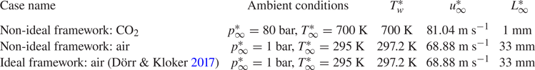
Stability diagram for cases described in table 3. Isocurves with  $\alpha _i=0, -0.3, -0.6,\ldots, -2.7$ are shown with different styles that fall on top of each other.

Appendix D. Comparison with a 2-D boundary layer
Recall the discussion on the modal behaviour in figure 13. We compare the result with an ad hoc case by setting  $w_s=0$ such that the boundary layer returns to 2-D. As shown in figure 23, the CF mode disappears when $w_s=0$ (green circles), while a new, inviscid TS-type mode is also observed. The phase velocity of this symmetrised mode matches the (asymmetric) one with true CF but has a larger growth rate. In other words, the CF somewhat stabilises the inviscid TS mode. Figure 23(c) shows similarities in the perturbation profiles, but the CF reduces the amplitudes of other perturbations ( $w^\prime$, $\rho ^\prime$, $T^\prime$) relative to $u^\prime$. Note also that there is no ‘viscous TS mode’ because the flow is accelerated; hence, no changeover from mode type I to II is possible, as in a zero-pressure gradient boundary layer.
Panels (a,b) are like figure 13(a,b), green circles correspond to the same baseflow but setting  ${w_s=0}$. (c) Baseflow ( $u_s$, $w_s$) and perturbation ( $|u^\prime |$, $|w^\prime |$, $|\rho ^\prime |$, $|T^\prime |$) profiles. Perturbations are compared for $w_s\neq 0$ (solid lines) and $w_s=0$ (dashed lines).


 Open access